Packet Switching Networksisg/NETWORKS/SLIDES/... · Dr. Indranil Sen Gupta Packet Switching...

Packet Switching Networks

Dr. Indranil Sen Gupta Packet Switching Networks Slide 1

Packet Switching (Basic Concepts)

• New form of architecture for long-distance data

communication (1970).

• Packet switching technology has evolved over time.

– basic technology has not changed


– basic technology has not changed

– packet switching remains one of the few effective technologies for

long-distance data communication.

Problems with Circuit Switching

• Network resources are dedicated to a particular connection.

• Two shortcomings for data communication.

– In a typical user/host data connection, line utilization is low.

– Provides facility for data transmission at a constant rate.


– Provides facility for data transmission at a constant rate.

• Data transmission pattern may not ensure this.

• Limits the utility of the method.

Packet Switching :: essential idea

• Data are transmitted in short packets (~ Kbytes).

– A longer message is broken up into a series of packets.

– Every packet contains some control information in its header

(required for routing and other purposes).


Message

HHH

Store-and-forward Concept

• Basic idea:

– Each network node receives and stores the packet,

– determines the next leg of the route, and

– queues the packet to go out on that link.


– queues the packet to go out on that link.

• Advantages:

– Line efficiency is greater (sharing of links).

– Data rate conversion is possible.

– Even under heavy traffic, packets are accepted, possibly with a

greater delivery delay.

– Packet priorities can be used.

Switching Technique

• As mentioned earlier, a packet switching network breaks

up a message into packets.

• Two contemporary approaches for handling these packets:

– Virtual Circuit


– Virtual Circuit

– Datagram

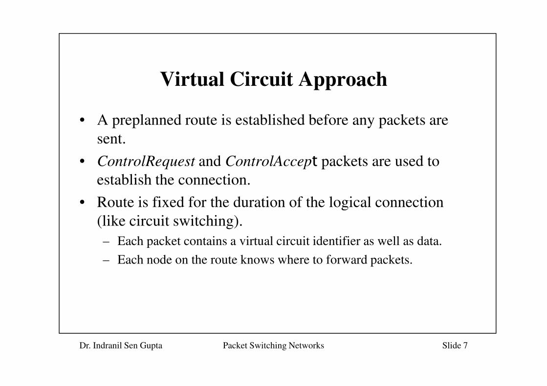
Virtual Circuit Approach

• A preplanned route is established before any packets are

sent.

• ControlRequest and ControlAccept packets are used to

establish the connection.

• Route is fixed for the duration of the logical connection


• Route is fixed for the duration of the logical connection

(like circuit switching).

– Each packet contains a virtual circuit identifier as well as data.

– Each node on the route knows where to forward packets.

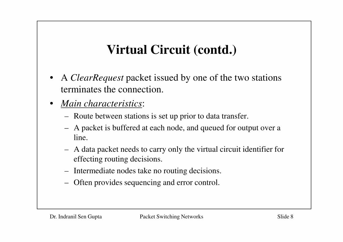
Virtual Circuit (contd.)

• A ClearRequest packet issued by one of the two stations

terminates the connection.

• Main characteristics:

– Route between stations is set up prior to data transfer.


– A packet is buffered at each node, and queued for output over a

line.

– A data packet needs to carry only the virtual circuit identifier for

effecting routing decisions.

– Intermediate nodes take no routing decisions.

– Often provides sequencing and error control.

Datagram Approach

• Each packet is treated independently, with no reference to

packets that have gone before.

• Every intermediate node has to take routing decisions.

– Every packet contains source and destination addresses.


– Intermediate nodes maintain routing tables.

• Problems:

– Packets may be delivered out of order.

– If a node crashes momentarily, all of its queued packets are lost.

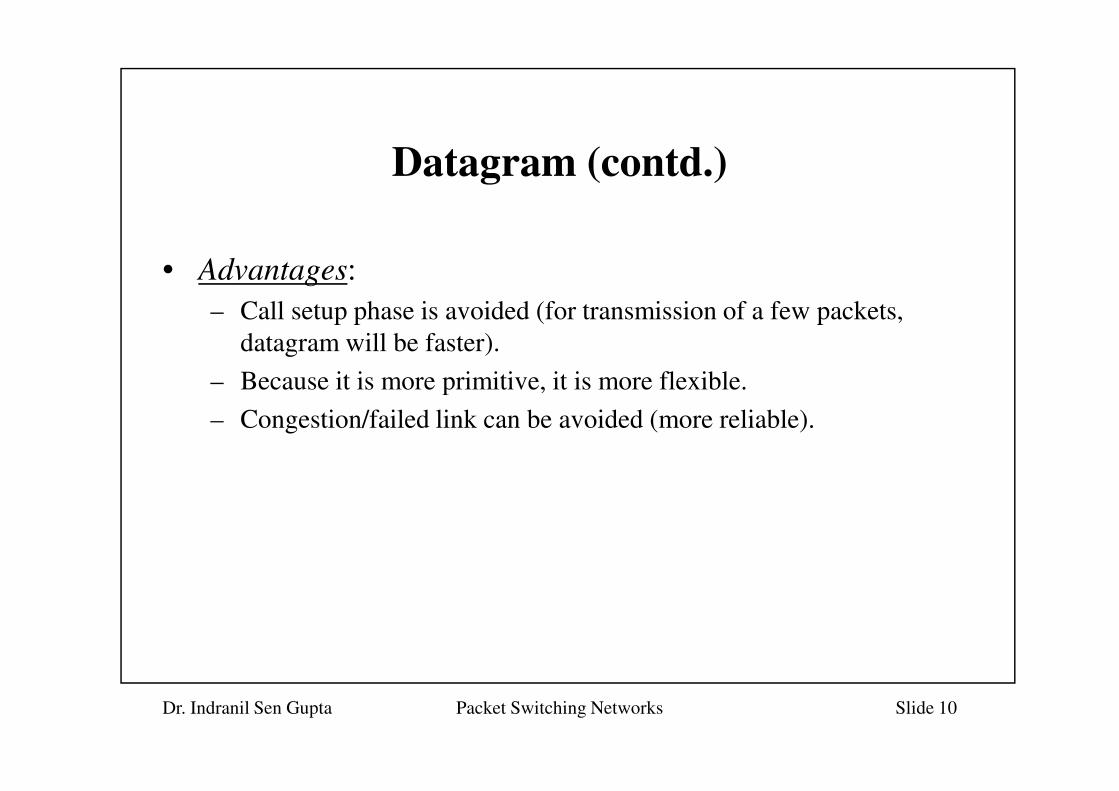
Datagram (contd.)

• Advantages:

– Call setup phase is avoided (for transmission of a few packets,

datagram will be faster).

– Because it is more primitive, it is more flexible.


– Congestion/failed link can be avoided (more reliable).

Effect of Packet

Size on

Transmission

Time


Contd.

• There is a significant relationship between packet size and

transmission time.

• Illustrative example:

– Assume there is a virtual circuit from station X through nodes a &

b to station Y.


b to station Y.

– Message size is 30 octets, packet header is 3 octets.

– 1-packet message ==> total 99 octet times




Comparison of Circuit & Packet Switching

• Three types of delays are encountered:

– Propagation Delay :: time taken by a signal to propagate from one

node to the next.

– Transmission Time :: time taken by the transmitter to send out a


block of data.

– Node Delay :: The time it takes for a node to perform the

necessary processing as it switches data.

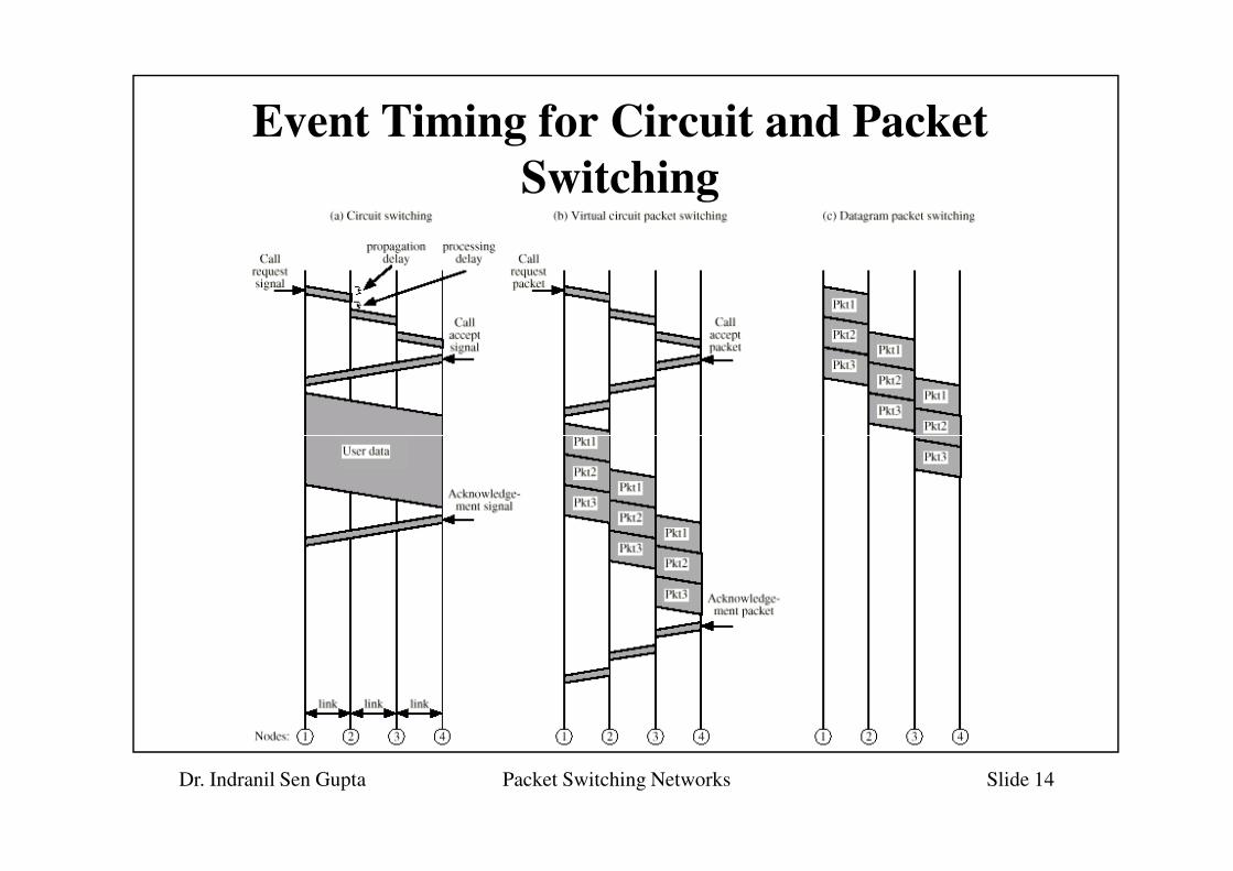
Event Timing for Circuit and Packet

Switching


External and Internal Operation

• Whether to use virtual circuit or datagram.

• Two dimensions to the problem:

– At the interface between a station and a network node, we may

have connection-oriented or connectionless service.


have connection-oriented or connectionless service.

– Internally, the network may use virtual circuits or datagrams.

• Leads to four different scenario (different VC/DG

combinations).

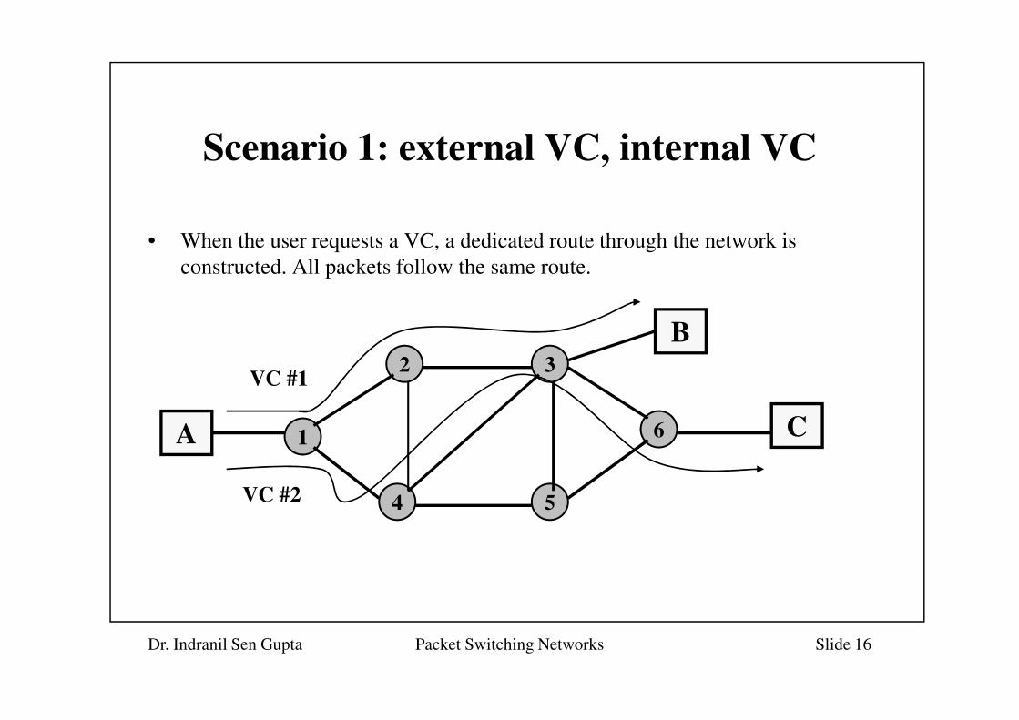
Scenario 1: external VC, internal VC

• When the user requests a VC, a dedicated route through the network is

constructed. All packets follow the same route.

2 3

B


1

2

4

3

5

6A C

VC #1

VC #2

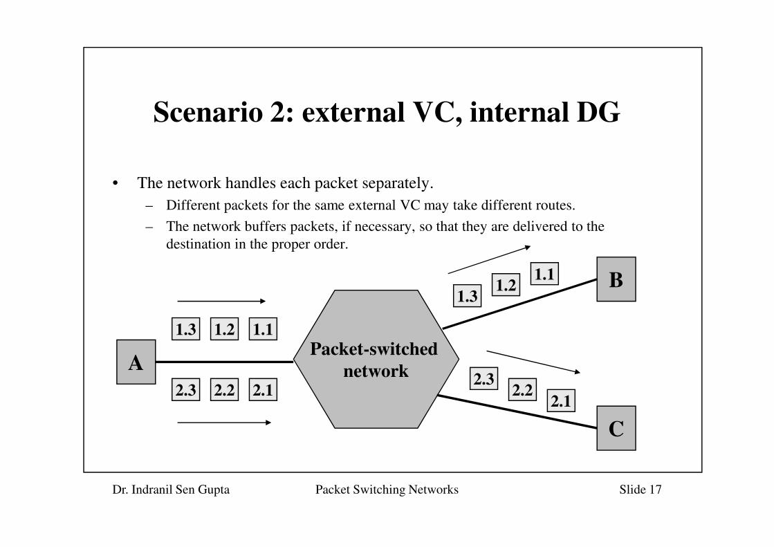
Scenario 2: external VC, internal DG

• The network handles each packet separately.

– Different packets for the same external VC may take different routes.

– The network buffers packets, if necessary, so that they are delivered to the

destination in the proper order.

B1.1


Packet-switched

networkA

B

C

1.3 1.2 1.1

2.3 2.2

1.3

2.1

1.21.1

2.3

2.12.2

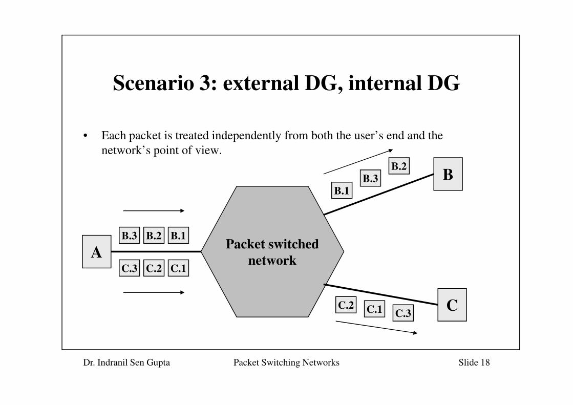
Scenario 3: external DG, internal DG

• Each packet is treated independently from both the user’s end and the

network’s point of view.

BB.1

B.2B.3


Packet switched

networkA

CC.3

B.2B.3 B.1

C.3 C.1C.2

C.1C.2

Scenario 4: external DG, internal VC

• The external user does not see any connections -- it simply sends packets one

at a time.

• The network sets up a logical connection between stations for packet delivery.

– May leave such connections in place for an extended period, so as to satisfy

anticipated future needs.


A

B

C3

2

3

112

3

Routing in Packet Switching Networks


Introduction

• One of the most complex and crucial aspect of packet-

switching network design is routing.

– In most subnets, packets will require multiple hops to make the

journey.


• Routing Algorithm:

– That part of the network layer software responsible for deciding

which output line an incoming packet should be transmitted on.

– For datagrams, this decision has to be taken for every arriving

packet.

– For virtual circuits, routing decisions are made only when a new

virtual circuit is being set up.

Desirable properties in a routing algorithm

• Correctness and simplicity: self-explanatory.

• Robustness: ability of the network to deliver packets via some route

even in the face of failures.

• Stability: the algorithm should converge to equilibrium fast in the

.


face of changing conditions in the network.

• Fairness and optimality: obvious requirements, but conflicting.

X

FDB

CA E

Y

X -> Y

A -> B

C -> D

E -> F

Performance Criteria

• The simplest criterion is to choose the minimum-hop route

through the network.

– Easily measured criterion.

• A generalization is least-cost routing.


• A generalization is least-cost routing.

– A cost is associated with each link.

– For any pair of attached stations, the least cost route through the

network is looked for.

• For either case, several well-known algorithms exists for

finding out the optimum path.

– Dijkstra’s algorithm

– Bellman-Ford algorithm

Routing Strategies

• A large number of routing strategies have evolved over the

years.

• Four key strategies shall be discussed:

– Fixed (Static) routing


– Fixed (Static) routing

– Flooding

– Random routing

– Adaptive routing

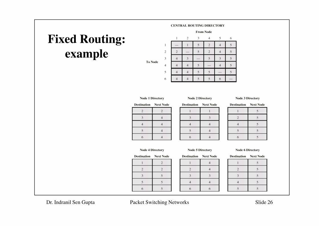
Fixed Routing

• A route is selected for each source-destination pair of nodes in the

network.

– Any standard least-cost routing algorithm can be used.

– The routes are fixed; they may only change if there is a change in the

topology of the network.

• How fixed routing may be implemented?


• How fixed routing may be implemented?

– A central routing matrix is created, which is stored at a network control

center.

– The matrix shows, for each source-destination pair of nodes, the identity

of the next node on the route.

– From the main routing matrix, routing tables to be used by each individual

node can be developed.

• Main advantage is simplicity, and works well in a reliable network

with stable load. Disadvantage is its lack of flexibility.

Fixed Routing:

example


Flooding

• Every incoming packet is sent out on every outgoing line

except the one it arrived on.

• Flooding generates vast number of duplicate packets, and

suitable damping mechanism must be used.


suitable damping mechanism must be used.

– A hop counter may be contained in the packet header, which is

decremented at each hop, with the packet being discarded when the

counter reaches zero.

• The sender initializes the hop counter. If no estimate is known, it is

set to the full diameter of the subnet.

– Keep track of which packets have been flooded, to avoid sending

them out a second time.

Flooding (contd.)

• A variation which is slightly more practical is

selective flooding.

– The routers do not send every incoming packet out on every line,

only on those lines that go in approximately the same direction.

• Utilities of flooding:


• Utilities of flooding:

– Flooding is highly robust, and could be used to send emergency

messages (e.g. military applications).

– May be used to initially set up the route in a virtual circuit.

• Flooding always chooses the shortest path, since it explores every

possible path in parallel.

– Can be useful for the dissemination of important information to all

nodes (e.g. routing information).

Random Routing

• This has the simplicity and robustness of flooding with far

less traffic load.

– A node selects only one outgoing path for retransmission of an

incoming packet.


– The outgoing link is chosen at random, excluding the link on

which the packet arrived.

• A refinement is to assign a probability to each outgoing

link and to select the link based on that probability.

• The actually route will typically not be the least-cost route.

– Network must carry a higher than optimum traffic load.

Adaptive Routing

• Routing decisions change as conditions on the network

change.

• Two principle conditions affecting routing decisions:

– Failure: When a node or trunk fails, it can no longer be used as part


– Failure: When a node or trunk fails, it can no longer be used as part

of the route.

– Congestion: When a particular portion of the network become

heavily congested, it is desirable to route packets around the area of

congestion.

• For adaptive routing to be possible, network state

information must be exchanged among the nodes.

– More information exchange ==> better routing ==> more overhead.

Adaptive Routing (contd.)

• Several drawbacks of the approach:

– Routing decision is more complex ==> more processing burden on

the switching nodes.

– Depends on status information that is collected at one place but


used at another ==> traffic overhead increases.

– It may react too quickly to changing network state, thereby

producing congestion-producing oscillation.

• Despite the drawbacks, adaptive routing is widely used.

– Improves performance, as seen by the network user.

– Can aid in congestion control.

Adaptive Routing Algorithms

• Several algorithms shall be discussed.

– Isolated adaptive routing.

– ARPANET: first generation.

– ARPANET: second generation.


– ARPANET: second generation.

– ARPANET: third generation.

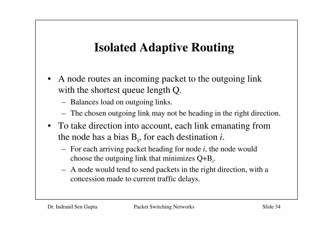
Isolated Adaptive Routing

• A node routes an incoming packet to the outgoing link

with the shortest queue length Q.

– Balances load on outgoing links.

– The chosen outgoing link may not be heading in the right direction.


– The chosen outgoing link may not be heading in the right direction.

• To take direction into account, each link emanating from

the node has a bias Bi, for each destination i.

– For each arriving packet heading for node i, the node would

choose the outgoing link that minimizes Q+Bi.

– A node would tend to send packets in the right direction, with a

concession made to current traffic delays.

Isolated Adaptive Routing: an example

Node 4’s Bias Table

for Destination 6

To 2


Next node Bias

1 9

2 6

3 3

5 0

To 1To 3

To 5

Packet arrives from node 1 ==> route through node 5

ARPANET: first generation

• Developed in 1969.

• Distributed adaptive algorithm using delay as the

performance criterion.

• Each node maintains two vectors:

– Di = [ di1 di2 …… din]


i i1 i2 in

– Si = [ si1 si2 ……. sin ]

– Here,

• Di is the delay vector for node i

• dij is the current estimate of minimum delay from node i to node j

• n is the number of nodes

• Si is the successor node vector for node i

• sij is the next node in the current minimum-delay route from i to j

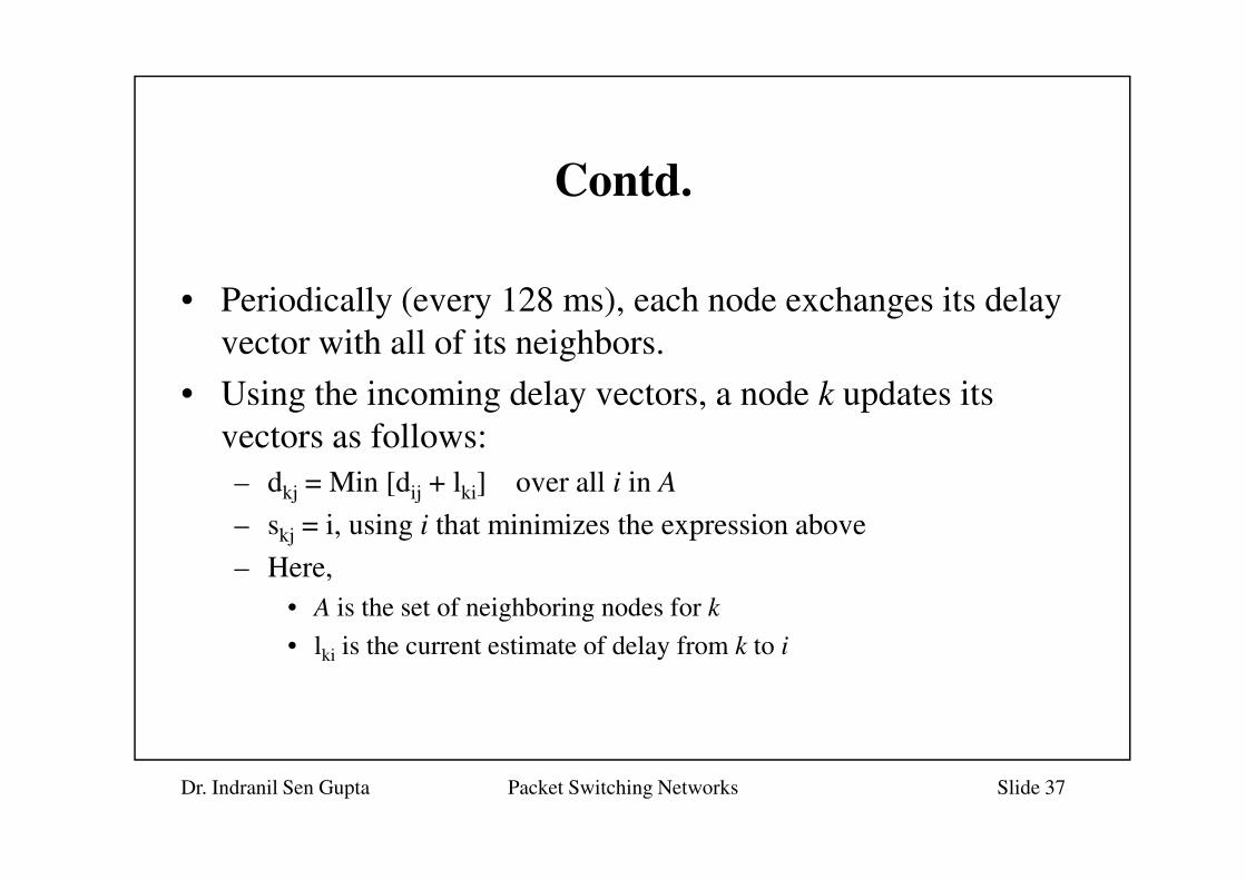
Contd.

• Periodically (every 128 ms), each node exchanges its delay

vector with all of its neighbors.

• Using the incoming delay vectors, a node k updates its

vectors as follows:


vectors as follows:

– dkj = Min [dij + lki] over all i in A

– skj = i, using i that minimizes the expression above

– Here,

• A is the set of neighboring nodes for k

• lki is the current estimate of delay from k to i

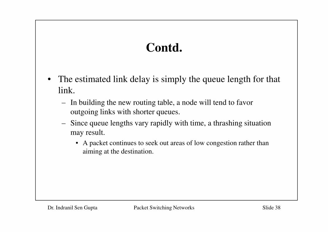
Contd.

• The estimated link delay is simply the queue length for that

link.

– In building the new routing table, a node will tend to favor

outgoing links with shorter queues.


– Since queue lengths vary rapidly with time, a thrashing situation

may result.

• A packet continues to seek out areas of low congestion rather than

aiming at the destination.

ARPANET: first generation

Illustrative Example


Figure 9.9 from the book by Stallings

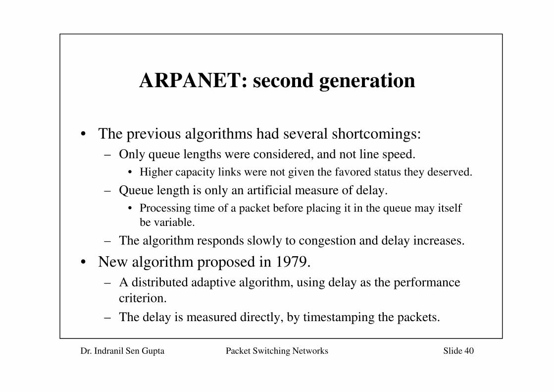
ARPANET: second generation

• The previous algorithms had several shortcomings:

– Only queue lengths were considered, and not line speed.

• Higher capacity links were not given the favored status they deserved.

– Queue length is only an artificial measure of delay.


– Queue length is only an artificial measure of delay.

• Processing time of a packet before placing it in the queue may itself

be variable.

– The algorithm responds slowly to congestion and delay increases.

• New algorithm proposed in 1979.

– A distributed adaptive algorithm, using delay as the performance

criterion.

– The delay is measured directly, by timestamping the packets.

ARPANET: third generation

• Problem with the previous approaches was that every node

was trying to obtain the best route for all destinations, and

that efforts conflicted.

• It was concluded that under heavy loads, the goal of

routing should be to give the average route a good path


routing should be to give the average route a good path

instead of attempting to give all routes the best path.

– The designers decided that it was unnecessary to change the

overall routing algorithm.

– It was sufficient to change the function that calculates link costs.

• Done in a way to damp routing oscillations and reduce routing

overheads.

• Uses simple concepts from queuing theory.

Congestion Control

• The objective is to maintain the number of packets in the

network below the level at which performance falls off

dramatically.

• Nature of a packet switching network.


• Nature of a packet switching network.

– A network of queues.

– At each node, there is a queue of packets for each outgoing channel.

– If packet arrival rate exceeds the packet transmission rate, the queue

size grows without bound.

– Rule of thumb: When the line for which packets are queuing becomes

more than 80% utilized, the queue length grows alarmingly.

What if packets arrive too fast?

• As packets arrive at a node, they are stored in an input buffer. If

packets arrive too fast, an incoming packet may find that there is no

available buffer space.

• One of two general strategies may be used:

– Simply discard any incoming packet for which there is no available buffer


– Simply discard any incoming packet for which there is no available buffer

space.

– The node that is experiencing these problems exercises some sort of flow

control over its neighbors so that the traffic flow remains manageable.

• In the second approach, if we try to regulate traffic flow, congestion at

one point of the network may quickly propagate to other parts of the

network.

Effect of congestionT

hro

ug

hp

ut

(pa

cket

s d

eliv

ered

)

Uncontrolled

Av

era

ge

pa

cket

del

ay


0.8 1.0

1.0

Uncontrolled

Controlled

Ideal

Offered Load (packets sent)

Th

rou

gh

pu

t (p

ack

ets

del

iver

ed)

Ideal

Controlled

0.8 1.0

Offered Load (packets sent)A

ver

ag

e p

ack

et d

ela

y

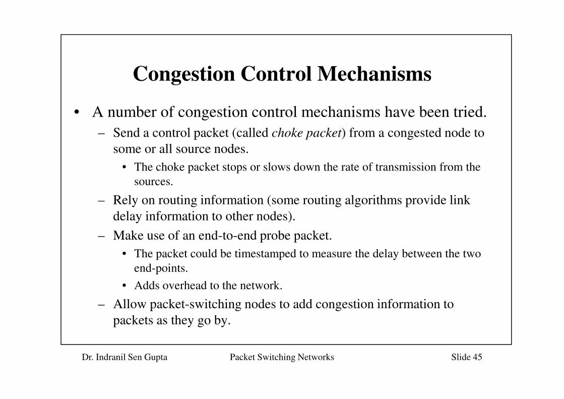
Congestion Control Mechanisms

• A number of congestion control mechanisms have been tried.

– Send a control packet (called choke packet) from a congested node to

some or all source nodes.

• The choke packet stops or slows down the rate of transmission from the

sources.

– Rely on routing information (some routing algorithms provide link


– Rely on routing information (some routing algorithms provide link

delay information to other nodes).

– Make use of an end-to-end probe packet.

• The packet could be timestamped to measure the delay between the two

end-points.

• Adds overhead to the network.

– Allow packet-switching nodes to add congestion information to

packets as they go by.

X.25

• Best known and most widely used packet switching

protocol standard.

– Originally approved in 1976.

– Subsequently revised in 1980, 1984, 1988, 1992, 1993.


– Subsequently revised in 1980, 1984, 1988, 1992, 1993.

• The standard specifies an interface between a host system

and a packet-switching network.

• Uses three layers of functionality:

– Physical layer

– Link layer

– Packet layer

X.25 Layers

• Physical Layer

– Deals with the physical interface between an attached station and the link that attaches that station to the packet-switching node.

• User machine termed as data terminal equipment (DTE)

• Packet switching node to which a DTE is attached is termed as data circuit-terminating equipment (DCE)

• X.21 is the most commonly used physical layer standard.


• X.21 is the most commonly used physical layer standard.

• Link Layer

– Provides for the reliable transfer of data across the physical link by transmitting the data as a sequence of frames.

– Link standard used is Link Access Protocol – balanced (LAPB), which is a subset of HDLC.

• Packet Layer

– Provides an external virtual-circuit service.

X.25 Interface

User ProcessTo remote user

process


Packet Packet

Link

Access

Link

Access

PhysicalPhysicalX.21 physical interface

LAPB

Multi-channel logical i/f

DTE DCE

X.25 Encapsulation


Figure 9.17 from the book by Stallings

X.25 Virtual Circuit Service

• With the X.25 packet layer, data are transmitted in packets

over external virtual circuits.

• X.25 provides two types of virtual circuit

– Virtual call: It is a dynamically established virtual circuit using a


– Virtual call: It is a dynamically established virtual circuit using a

call setup and call termination procedure.

– Permanent virtual circuit: It is a fixed, network-assigned virtual

circuit.

• Data transfer occurs as with virtual calls

• No call setup or termination is required.

X.25 Packet Format

• User data are broken into blocks of some maximum size, and a 24-bit

or 32-bit header is appended to each block to form a data packet.

• Uses sliding-window protocol with piggybacking

– Go-back-N for error control.

• X.25 also transmits control packets related to the establishment,

maintenance and termination of virtual circuits.


maintenance and termination of virtual circuits.

– Each control packet includes:

• The virtual circuit number.

• The packet type (call request, call accepted, call confirm, interrupt, reset,

restart, etc.).

• Additional control information specific to the type of packet.

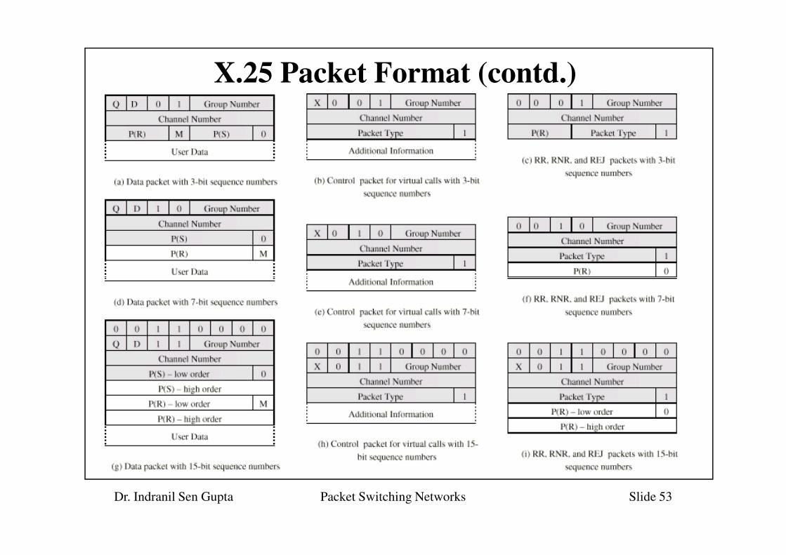
X.25 Packet Format (contd.)


X.25 Multiplexing

• One of the most important services provided by X.25.

– A DTE is allowed to establish up to 4095 simultaneous virtual

circuits with other DTEs over a single DTE-DCE link.

– Each packet contains a 12-bit virtual circuit number.


• Expressed as a 4-bit logical group number plus an 8-bit logical

channel number.

– Individual virtual circuits could correspond to applications,

processes, terminals, etc.

– The DTE-DCE link provides full-duplex multiplexing.

Packet Switching Networksisg/NETWORKS/SLIDES/... · Dr. Indranil Sen Gupta Packet Switching...

Documents

Transcript of Packet Switching Networksisg/NETWORKS/SLIDES/... · Dr. Indranil Sen Gupta Packet Switching...