Package-X: A Mathematica package for the analytic calculation of one-loop integrals

Hiren H. Patel1, ∗

1Particle and Astro-Particle Physics DivisionMax-Planck Institut fuer Kernphysik (MPIK)Saupfercheckweg 1, 69117 Heidelberg, Germany

Package-X, a Mathematica package for the analytic computation of one-loop integrals dimension-ally regulated near 4 spacetime dimensions is described. Package-X computes arbitrarily high ranktensor integrals with up to three propagators, and gives compact expressions of UV divergent, IRdivergent, and finite parts for any kinematic configuration involving real-valued external invariantsand internal masses. Output expressions can be readily evaluated numerically and manipulatedsymbolically with built-in Mathematica functions. Emphasis is on evaluation speed, on readabil-ity of results, and especially on user-friendliness. Also included is a routine to compute traces ofproducts of Dirac matrices, and a collection of projectors to facilitate the computation of fermionform factors at one-loop. The package is intended to be used both as a research tool and as aneducational tool.

Program summary

Program title: Package-X

Program obtainable from: CPC Program Library, Queen’s University, Belfast, N. Ireland, orhttp://packagex.hepforge.org

Licensing provisions: Standard CPC license, http://cpc.cs.qub.ac.uk/licence/licence.html

Programming language: Mathematica (Wolfram Languange)

Operating systems: Windows, Mac OS X, Linux (or any system supporting Mathematica 8.0 orhigher)

RAM required for execution: 10 MB, depending on size of computation

Vectorised/parallelized?: No

Nature of problem: Analytic calculation of one-loop integrals in relativistic quantum field theoryfor arbitrarily high-rank tensor integrals and any kinematic configuration of real-valued externalinvariants and internal masses.

Solution method: Passarino-Veltman reduction formula, Denner-Dittmaier reduction formulae, andtwo new reduction algorithms described in the manuscript.

Restrictions: One-loop integrals are limited to those involving no more than three propagator fac-tors.

Unusual features: Includes rudimentary routines for tensor algebraic operations and for performingtraces over Dirac gamma matrices.

Running Time: 5ms to 10s for integrals typically occurring in practical computations; longer forhigher rank tensor integrals.

I. INTRODUCTION

Many packages are available to assist with the evalu-ation of one-loop integrals that appear in higher ordercalculations of perturbative quantum field theory. Themost widely used ones are the Mathematica packagesFeynCalc[1], FormCalc[2] and the Fortran programGolem95[3]. These packages compute one-loop inte-grals using the Passarino-Veltman reduction algorithm[4]

∗ hiren.patel@mpi-hd.mpg.de

(FeynCalc and FormCalc also feature a collection ofroutines designed to streamline the numerical computa-tion of a differential cross section; as such, they do sub-stantially more than to simply compute one-loop inte-grals).

Nevertheless FeynCalc falls short in that it gives re-sults of one-loop computations in terms of basis scalarfunctions which cannot be evaluated on their own. In-stead, it is up to the user to supply their analyti-cal forms from an external source, or to link them toyet another package (such as FF[5], LoopTools[2], orOneLOop[6]).

Moreover, one-loop integrals have many more applica-

arX

iv:1

503.

0146

9v2

[he

p-ph

] 4

Sep

201

5

2

tions than to calculate cross sections and decay rates. Ex-amples are the computation of ultraviolet counterterms,pole positions, residues, Peskin-Takeuchi oblique param-eters, electromagnetic moments, etc. Many of these ap-plications require the calculation of Feynman integralsat singular kinematic points such as at physical thresh-olds or zero external momenta. Since the Passarino-Veltman reduction algorithm typically breaks down atthese points, it is nearly impossible to obtain results with

FeynCalc or FormCalc (Golem95 can give numeri-cal results). But, it is also at these points where compactanalytic expressions exist.

Although smaller-scale packages are available that aredesigned around a particular application (such as lool[7]and ant[8]), there is no general-purpose software thatgives analytic results to one-loop integrals for all kine-matic configurations. In this regard, Package-X serves tofill this gap.

Package-X calculates dimensionally regulated (d = 4− 2ε) rank-P one-loop tensor integrals of the form

Tµ1...µPN (p1, . . . , pN ;m0,m1 . . . ,mN ) = µ2ε

∫ddk

(2π)dkµ1 · · · kµP

[k2−m20+iε][(k+p1)2−m2

1+iε] · · · [(k+pN )2−m2N+iε]

, (1)

with up toN = 3 denominator factors, and finds compactanalytic expressions for arbitrary configurations of exter-nal momenta pi and real-valued internal masses mi. Thefunctional paradigm of the Wolfram Language togetherwith the supplementary trace-taking routines includedin Package-X allows one to compute an entire one-loopdiagram at once. All output is ready for numerical eval-uation and symbolic manipulation with Mathematica’sinternal functions.

This article details the technical aspects of Package-X, and assumes familiarity in the use of the package.The application files are found at the Hepforge web-page http://packagex.hepforge.org, where the soft-ware will be maintained and periodically updated. In-cluded among the package files is a tutorial that providesan introduction, and a complete set of documentationfiles that becomes embedded with the Wolfram Docu-mentation Center upon installation which provides de-tails and examples of all functions defined in Package-X.

II. STRUCTURE AND DESIGN OF PACKAGE

The subroutines in this package belong to one ofthree Mathematica contexts organized as in Fig. 1.The module IndexAlg‘ contains the rudimentary tensor-algebraic routines and serves as the backbone of Package-X. OneLoop‘ contains the algorithms and look-up tablesfor the computation of one-loop integrals, and Spur‘ in-cludes the algorithms to perform traces over products ofDirac matrices and contains a catalog of fermion formfactor projectors.

The basic Package-X workflow for the computation ofa one-loop integral consists of three steps:

1. Call LoopIntegrate to carry out the covariant ten-sor decomposition (section III).

2. Apply on-shell conditions and other kinematicrelations with Mathematica’s built-in functionsReplaceAll (/.) and Rules (→).

IndexAlg`LTensorLDot

OneLoop`LoopIntegrateLoopRefine

Spur`SpurProjector

FIG. 1. Organization of functions into contexts as defined inPackage-X.

3. Call LoopRefine to convert coefficient functionsinto explicit expressions (section IV).

The reasoning behind the three-step design is as follows:kinematic configurations of external invariants pi.pj andinternal massesmi relevant to many physical applicationsoccur at singular points of one-loop integrals, such thatif they were applied after obtaining the general expres-sions, errors like 0/0 or 0× ln(0) would inevitably occur.To avoid such errors and to facilitate the generation ofcompact results, LoopRefine uses algorithms dependingcritically on the kinematic configuration supplied by theuser beforehand.

Two other supplementary functions are provided tostreamline computations involving fermions:

• Spur (German for ‘trace’ ) computes traces of Diracmatrices that may appear in the numerators of one-loop integrals (section VII).

• Projector is used to project fermion self-energyand vertex form factors out of the loop integrals(section VIII).

The algorithms used by these functions are detailed inthe aforementioned sections below.

3

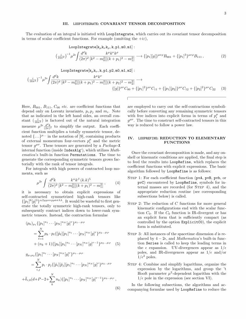
III. LOOPINTEGRATE: COVARIANT TENSOR DECOMPOSITION

The evaluation of an integral is initiated with LoopIntegrate, which carries out its covariant tensor decompositionin terms of scalar coefficient functions. For example (omitting the +iε),

LoopIntegrate[kµkνkρ, k, p1, m0, m1] :(i

16π2

)−1µ2ε

∫ddk

(2π)dkµkνkρ

[k2 −m20][(k + p1)2 −m2

1]−→ {[p1][g]}µνρB001 + {[p1]3}µνρB111 , (2)

LoopIntegrate[kµkν , k, p1, p2, m0, m1, m2] :(i

16π2

)−1µ2ε

∫ddk

(2π)dkµkν

[k2 −m20][(k + p1)2 −m2

1][(k + p2)2 −m22]−→

{[g]}µνC00 + {[p1]2}µνC11 + {[p1][p2]}µνC12 + {[p2]2}µνC22 (3)

Here, B001, B111, C00 etc. are coefficient functions thatdepend only on Lorentz invariants, pi.pj and mi. Notethat as indicated in the left hand sides, an overall con-stant ( i

16π2 ) is factored out of the natural integration

measure µ2ε ddk(2π)d

to simplify the output. Each coeffi-

cient function multiplies a totally symmetric tensor, de-noted {. . .}µ... in the notation of [9], containing productsof external momentum four-vectors pµi and the metrictensor gµν . These tensors are generated by a Package-Xinternal function (inside IndexAlg‘), which utilizes Math-ematica’s built-in function Permutations. The time togenerate the corresponding symmetric tensors grows fac-torially with the rank of tensor integrals.

For integrals with high powers of contracted loop mo-menta, such as

µ2ε

∫ddk

(2π)dkαkβ (k.k)5

[k2 −m20][(k + p1)2 −m2

1], (4)

it is necessary to obtain explicit expressions ofself-contracted symmetrized high-rank tensors like{[p1]6[g]3}αβµµννρρσσλλ. It would be wasteful to first gen-erate the totally symmetric high-rank tensors, only tosubsequently contract indices down to lower-rank sym-metric tensors. Instead, the contraction formulae

(pk)µ1{[p1]n1 · · · [pN ]nN [g]r}µ1...µP

=

N∑`=1

pk · p`{[p`][p1]n1 · · · [pN ]nN [g]r}µ2...µP

+ (nk + 1){[pk][p1]n1 · · · [pN ]nN [g]r−1}µ2...µP (5)

gµ1µ2{[p1]n1 · · · [pN ]nN [g]r}µ1...µP

=

N∑i,j

pi · pj{[pi][pj ][p1]n1 · · · [pN ]nN [g]r}µ3...µP

+δr,0(d+P−2+

N∑k

nk){[p1]n1 · · · [pN ]nN [g]r−1}µ3...µP ,

(6)

are employed to carry out the self-contractions symboli-cally before converting any remaining symmetric tensorswith free indices into explicit forms in terms of pµi andgµν . The time to construct self-contracted tensors in thisway is reduced to follow a power law.

IV. LOOPREFINE: REDUCTION TO ELEMENTARYFUNCTIONS

Once the covariant decomposition is made, and any on-shell or kinematic conditions are applied, the final step isto feed the results into LoopRefine, which replaces thecoefficient functions with explicit expressions. The basicalgorithm followed by LoopRefine is as follows:

Step 1: For each coefficient function (pvA, pvB, pvb, orpvC) encountered by LoopRefine, symbols for in-ternal masses are recorded (for Step 4), and theappropriate reduction routine (see correspondingsubsections below) is called.

Step 2: The reduction of C functions for more generalkinematic configurations end with the scalar func-tion C0. If the C0 function is IR-divergent or hasan explicit form that is sufficiently compact (ascontrolled by the option ExplicitC0), the explicitform is substituted.

Step 3: All instances of the spacetime dimension d is re-placed by 4− 2ε, and Mathematica’s built-in func-tion Series is called to keep the leading terms inthe ε expansion. UV-divergences appear as 1/εpoles, and IR-divergences appear as 1/ε and/or1/ε2 poles.

Step 4: Combine and simplify logarithms, organize theexpression by the logarithms, and group the ’tHooft parameter µ2-dependent logarithm with the1/ε pole in the expression (see section VI).

In the following subsections, the algorithms and ac-companying formulae used by LoopRefine to reduce the

4

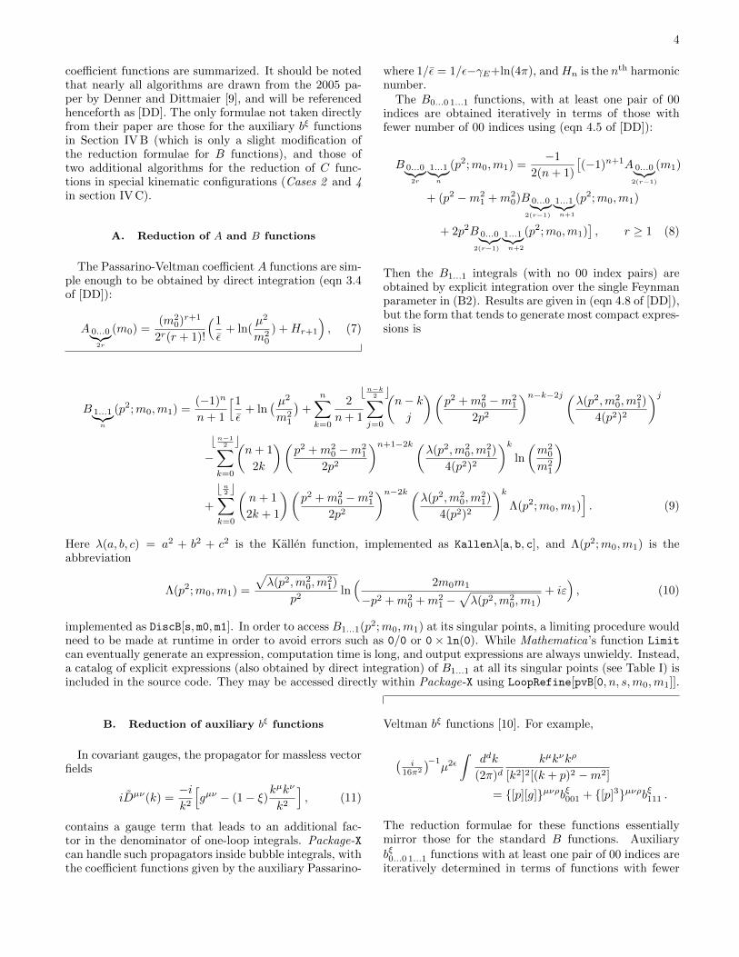
coefficient functions are summarized. It should be notedthat nearly all algorithms are drawn from the 2005 pa-per by Denner and Dittmaier [9], and will be referencedhenceforth as [DD]. The only formulae not taken directlyfrom their paper are those for the auxiliary bξ functionsin Section IV B (which is only a slight modification ofthe reduction formulae for B functions), and those oftwo additional algorithms for the reduction of C func-tions in special kinematic configurations (Cases 2 and 4in section IV C).

A. Reduction of A and B functions

The Passarino-Veltman coefficient A functions are sim-ple enough to be obtained by direct integration (eqn 3.4of [DD]):

A 0...0︸︷︷︸2r

(m0) =(m2

0)r+1

2r(r + 1)!

(1

ε+ ln(

µ2

m20

) +Hr+1

), (7)

where 1/ε = 1/ε−γE+ln(4π), andHn is the nth harmonicnumber.

The B0...0 1...1 functions, with at least one pair of 00indices are obtained iteratively in terms of those withfewer number of 00 indices using (eqn 4.5 of [DD]):

B 0...0︸︷︷︸2r

1...1︸︷︷︸n

(p2;m0,m1) =−1

2(n+ 1)

[(−1)n+1A 0...0︸︷︷︸

2(r−1)

(m1)

+ (p2 −m21 +m2

0)B 0...0︸︷︷︸2(r−1)

1...1︸︷︷︸n+1

(p2;m0,m1)

+ 2p2B 0...0︸︷︷︸2(r−1)

1...1︸︷︷︸n+2

(p2;m0,m1)], r ≥ 1 (8)

Then the B1...1 integrals (with no 00 index pairs) areobtained by explicit integration over the single Feynmanparameter in (B2). Results are given in (eqn 4.8 of [DD]),but the form that tends to generate most compact expres-sions is

B 1...1︸︷︷︸n

(p2;m0,m1) =(−1)n

n+ 1

[1

ε+ ln

( µ2

m21

)+

n∑k=0

2

n+ 1

bn−k2 c∑j=0

(n− kj

)(p2 +m2

0 −m21

2p2

)n−k−2j (λ(p2,m2

0,m21)

4(p2)2

)j

−bn−1

2 c∑k=0

(n+ 1

2k

)(p2 +m2

0 −m21

2p2

)n+1−2k (λ(p2,m2

0,m21)

4(p2)2

)kln

(m2

0

m21

)

+

bn2 c∑k=0

(n+ 1

2k + 1

)(p2 +m2

0 −m21

2p2

)n−2k (λ(p2,m2

0,m21)

4(p2)2

)kΛ(p2;m0,m1)

]. (9)

Here λ(a, b, c) = a2 + b2 + c2 is the Kallen function, implemented as Kallenλ[a, b, c], and Λ(p2;m0,m1) is theabbreviation

Λ(p2;m0,m1) =

√λ(p2,m2

0,m21)

p2ln( 2m0m1

−p2 +m20 +m2

1 −√λ(p2,m2

0,m1)+ iε

), (10)

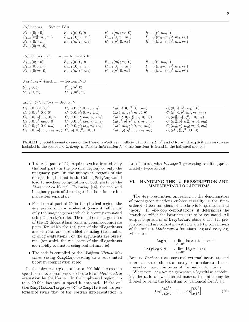
implemented as DiscB[s, m0, m1]. In order to access B1...1(p2;m0,m1) at its singular points, a limiting procedure wouldneed to be made at runtime in order to avoid errors such as 0/0 or 0× ln(0). While Mathematica’s function Limitcan eventually generate an expression, computation time is long, and output expressions are always unwieldy. Instead,a catalog of explicit expressions (also obtained by direct integration) of B1...1 at all its singular points (see Table I) isincluded in the source code. They may be accessed directly within Package-X using LoopRefine[pvB[0, n, s,m0,m1]].

B. Reduction of auxiliary bξ functions

In covariant gauges, the propagator for massless vectorfields

iDµν(k) =−ik2

[gµν − (1− ξ)k

µkν

k2

], (11)

contains a gauge term that leads to an additional fac-tor in the denominator of one-loop integrals. Package-Xcan handle such propagators inside bubble integrals, withthe coefficient functions given by the auxiliary Passarino-

Veltman bξ functions [10]. For example,

(i

16π2

)−1µ2ε

∫ddk

(2π)dkµkνkρ

[k2]2[(k + p)2 −m2]

= {[p][g]}µνρbξ001 + {[p]3}µνρbξ111 .

The reduction formulae for these functions essentiallymirror those for the standard B functions. Auxiliary

bξ0...0 1...1 functions with at least one pair of 00 indices areiteratively determined in terms of functions with fewer

5

00 index pairs using

bξ0...0︸︷︷︸2r

1...1︸︷︷︸n

(p2;m) =−1

2(n+ 1)

[B 0...0︸︷︷︸

2(r−1)

(p2; 0,m)

+ (p2 −m2)bξ0...0︸︷︷︸2(r−1)

1...1︸︷︷︸n+1

(p2;m)

+ 2p2bξ0...0︸︷︷︸2(r−1)

1...1︸︷︷︸n+2

(p2;m)], r ≥ 1 , (12)

and the bξ1...1 functions with no 00 index pairs are ob-tained by direct integration over the single Feynman pa-rameter in (B3). The integral is finite if n ≥ 1, with theresult

bξ1...1︸︷︷︸n

(p2;m) =

(−1)n−1

p2

[− 1

n+n−1∑k=1

1

n− km2

p2 −m2

(p2 −m2

p2

)k+

m2

p2 −m2

(p2 −m2

p2

)nln

(m2

m2 − p2+ iε

)].

If n = 0 (a case that is not met in practice since the gaugepart of the spin-1 propagator guarantees two powers ofmomenta in the numerator), the auxiliary bξ function isIR-divergent.

Explicit expressions at the various singular points of

bξ1...1 (see Table I) are included in the Package-X sourcecode.

C. Reduction of C functions

The reduction of coefficient C functions is significantlycomplicated by its numerous singular points. Althoughthe standard Passarino-Veltman reduction algorithm isapplicable at almost all points (Case 1 below), differ-ent formulae are needed to handle the various singularcases (Cases 2 – 6 ). LoopRefine identifies the nature ofthe kinematic configuration and applies the appropriatereduction method.

Cases 1, 3, 5 and 6 are taken from [DD]. Note thatsince the emphasis of [DD] is on numerical stability andnot on generating analytic expressions, the algorithmspresented there do not automatically give compact ex-pressions. The algorithm under Case 2 is new, and whiletechnically it is covered by Case 1, it leads to more com-pact expressions. Furthermore, an algorithm to handlethe reduction at physical thresholds (applied in Case 3below) is not completely covered by [DD]. This gap isfilled by the formulae under Case 4.

The arguments of the coefficient C functions are or-dered differently in Package-X as compared to those usedby other authors. See Appendix A for details.

In the reduction formulae below, the following kine-matic abbreviations are used (which differ slightly from[DD] by numeric factors):

fj = p2j −m2

j +m20 , j = {1, 2}

Z =

(p2

1 p1.p2

p2.p1 p22

)(Gramian matrix)

q2 = p21 + p2

2 − 2p1.p2

detZ = 14λ(q2, p2

1, p22)

Z =

(p2

2 −p1.p2

−p1.p2 p21

)(cofactor matrix)

X0j =

(p2

2f1 − p1.p2f2

−p1.p2f1 + p21f2

)j = {1, 2}

(13)

Furthermore, hatted indices on coefficient functions (e.g.Bk0...0 1...1) indicate the removal of those indices. Co-efficient B functions derived by canceling denominatorsfrom three-point integrals are abbreviated by

B...(D1) =B...(p22;m0,m2) (14)

B...(D2) =B...(p21;m0,m1) . (15)

If the denominator (k2−m20)−1 independent of an exter-

nal momentum vector is cancelled, a shifted form of theB function is used:

B 0...0︸︷︷︸2r

1...1︸︷︷︸n1

2...2︸︷︷︸n2

(D0) =

(−1)n1

n1∑j=0

(n1

j

)B 0...0︸︷︷︸

2r

1...1︸︷︷︸n2+j

(q2;m1,m2) . (16)

Whenever n1 > n2 the invariance property

B 0...0︸︷︷︸2r

1...1︸︷︷︸n1

2...2︸︷︷︸n2

(D0) = B 0...0︸︷︷︸2r

1...1︸︷︷︸n2

2...2︸︷︷︸n1

(D0)∣∣∣m1↔m2

(17)

is used to keep the number of terms in the sum to aminimum. Cases 2 and 4 require expressions for the Bfunctions with the number of 00 index pairs continued tor = −1. Details of this function are found in AppendixE.

Finally, formulae for Cases 1, 3 and 5 below containexplicit dependence on spacetime dimension d = 4 − 2εappearing in denominators of certain prefactors. In thecourse of reduction, the O(ε) part multiplying any lowercoefficient functions combines with their UV 1/ε poles1,and gives rise to finite polynomials in kinematic variables.Although this can be automatically handled by Seriesat Step 3, the reduction algorithm performs much fasterif these polynomials are explicitly supplied. They areobtained by integration over the Feynman parameters asdescribed at the end of Appendix B.

6

Case 1: detZ 6= 0

At non-singular kinematic configurations with detZ 6= 0, the original [4] Passarino-Veltman reduction formula isused (eqns 5.10, 5.11 of [DD]):

C 0...0︸︷︷︸2r

1...1︸︷︷︸n1

2...2︸︷︷︸n2

=1

2 detZ

2∑k=1

Zjk

[δnk,δjkB 0...0︸︷︷︸

2r

1...1︸︷︷︸nk−δ

k1

(Dk)−B 0...0︸︷︷︸2r

1...1︸︷︷︸n1−1

2...2︸︷︷︸n2

(D0)

− fkC 0...0︸︷︷︸2r

1...1︸︷︷︸n1−1

2...2︸︷︷︸n2

(D0)− 2(nk − δjk)Ck 0...0︸︷︷︸2r+2

1...1︸︷︷︸n1−1

2...2︸︷︷︸n2

], n1 ≥ 1

C 0...0︸︷︷︸2r

=1

2(d− 4 + 2r)

[B 0...0︸︷︷︸

2r−2

(D0) + 2m20C 0...0︸︷︷︸

2r−2

1 + f2C 0...0︸︷︷︸2r−1

2

], r ≥ 1

(18)

where k =

{1 , k = 2

2 , k = 1. In the first equation, j = 1 is taken, although the choice j = 2 would give equivalent results.

If n1 = 0 with n2 > 0, then the relation (B5) is used and the first equation is applied.

Case 2: Ellis-Zanderighi triangle 6

Coefficient C functions for which arguments are (m20, s,m

22;m2, 0,m0)—or an equivalent permutation thereof—are

already covered by Case 1. However, final expressions obtained from it tend not to give the most compact formulaefor this kinematic configuration. More compact formulae are obtained by directly integrating over the Feynmanparameters in (B4); see Appendix C for derivation. It is of note that the corresponding scalar function C0 is theIR-divergent three-point function, ‘triangle 6’, as classified by Ellis and Zanderighi [11]. In Eqs. (19) and (20), it isassumed that at least one of r, n1 or n2 is nonzero.

C 0...0︸︷︷︸2r

1...1︸︷︷︸n1

2...2︸︷︷︸n2

(m20, s,m

22;m2, 0,m0) =

(−1)n1

2

n1!(n2 + 2r − 1)!

(n1 + n2 + 2r)!

(1 + 2ε(Hn1+n2+2r −Hn2+2r−1)

)B 0...0︸︷︷︸

2r−2

1...1︸︷︷︸n2

(s;m0,m2) ,

n2 6= 0 or r 6= 0

C 1...1︸︷︷︸n1

(m20, s,m

22;m2, 0,m0) =

(−1)n1

[C0(m2

0, s,m22;m2, 0,m0)− 1

2

(Hn1

+ ε(H2n1

+H(2)n1

))B 0...0︸︷︷︸−2

(s;m0,m2)]

(19)

where H(r)n is the nth harmonic number of order r. If the arguments take the form (s,m2

0,m22; 0,m2

2,m0), then theidentity (B5) is applied, and the equations above are valid.

A different formula is needed if the off-shell momentum s is in the third position:

C 0...0︸︷︷︸2r

1...1︸︷︷︸n1

2...2︸︷︷︸n2

(m22,m

20, s;m0,m2, 0) =

(−1)n2

2

1

n1 + n2 + 2r

n2∑k=0

(n2

k

)(1+

2ε

n1 + n2 + 2r

)B 0...0︸︷︷︸

2r−2

1...1︸︷︷︸n1+k

(s;m0,m2) (20)

To apply Eqs. (19) and (20) above, explicit forms of the scalar B function with the number of 00 index pairs takento r = −1 is occasionally needed. These functions are discussed in Appendix E.

1 For the argument that they are only of UV origin (and not IR),see the argument in Sec. 5.8 of [DD]

7

Case 3: detZ = 0 but X0j 6= 0

With detZ = 0, the primary reduction formulae are rearranged to give: (eqns 5.38 and 5.40 of [DD])

C 0...0︸︷︷︸2r

=1

d+ 2r − 3

(B 0...0︸︷︷︸

2r−2

(D0)−m20C 0...0︸︷︷︸

2r−2

)+

1

2(d+ 2r − 3)Zkl

2∑n,m=1

(δkmδnl − δklδnm

)

×{ 2∑j=1

Znj

[(1− δmj)B 0...0︸︷︷︸

2r−2

1(Dm)−Bj 0...0︸︷︷︸2r−2

(D0)]

+1

2fm

[−B 0...0︸︷︷︸

2r−2

(Dn) +B 0...0︸︷︷︸2r−2

(D0) + fnC 0...0︸︷︷︸2r−2

]}r > 0

C 0...0︸︷︷︸2r

1...1︸︷︷︸n1

2...2︸︷︷︸n2

=1

X0j

2∑k=1

Zjk

(δnk0B 0...0︸︷︷︸

2r

1...1︸︷︷︸nk

(Dk)−B 0...0︸︷︷︸2r

1...1︸︷︷︸n1

2...2︸︷︷︸n2

(D0)− 2nkCk00 0...0︸︷︷︸2r

1...1︸︷︷︸n1

2...2︸︷︷︸n2

)(21)

The value of j chosen (1 or 2) is the one for which the corresponding X0j is non-vanishing. If both elements arevanishing, then Case 4 is applied. Note that the second relation is valid even when either n1 = 0 or n2 = 0. Inparticular, when r = n1 = n2 = 0 the final term in that relation vanishes, and leads to the reduction of the scalar C0

function in terms of scalar B0 functions.

Case 4: vanishing detZ and X0j

When the physical threshold (corresponding to X0j = 0 for both j = {1, 2}) coincides with the boundary ofthe physical region (detZ = 0), then Cases 1—3 are inapplicable. For this kinematic configuration, the reductionformulae in [DD] eqns (5.49) and (5.53) can be used provided at least one element of

Xij =

(4m2

0p22 − f2

2 −2m20(p2

1 + p22 − q2) + f1f2

−2m20(p2

1 + p22 − q) + f1f2 4m2

0p21 − f2

1

)is non-vanishing. However, no reduction methods are presented in [DD] that are valid when all four elements of Xij

are vanishing, because an expansion around that point is not known2. This exceptional configuration is needed for thecomputation of elastic form factors at zero momentum such as electron g − 2. To fill this gap, a new set of reductionformulae are used that is valid regardless of the form of Xij , provided at least one of p2

1, p22 or q2 is non-vanishing.

These formulae are derived in Appendix D.If p2

2 6= 0,

C 0...0︸︷︷︸2r

1...1︸︷︷︸n1

2...2︸︷︷︸n2

=(−1)n1+n2

2

n2∑j=0

(n2

j

)αn2−j

{n1!(n2 − j)!

(n1 + n2 − j + 1)!

j∑k=0

[(j

k

)(−α)j−k(−1)kB 0...0︸︷︷︸

2r−2

1...1︸︷︷︸k

(D1)

]

+

n1∑k=0

(−1)n2

n2 − j + k + 1

(n1

k

)[(1− α)j+1(−1)n2B 0...0︸︷︷︸

2r−2

1...1︸︷︷︸n2+k+1

(D0)− (−α)j+1B 0...0︸︷︷︸2r−2

1...1︸︷︷︸n2+k+1

(D2)]}

, (22)

where α = −q2 + p21 + p2

2/(2p22).

If p22 = 0, then detZ = 0 implies q2 = p2

1, and the formula

C 0...0︸︷︷︸2r

1...1︸︷︷︸n1

2...2︸︷︷︸n2

=(−1)n1+1

2(n2 + 1)

n1∑k=0

(n1

k

)B 0...0︸︷︷︸

2r−2

1...1︸︷︷︸n2+k+1

(D2) (23)

is used. If p21 = p2

2 = q2 = 0, then these formulae are inapplicable and Case 5 is needed. Note that when r = 0 ineither (22) or (23), the B functions continued to r = −1 are needed (see Appendix E).

2 A. Denner, private correspondence

8

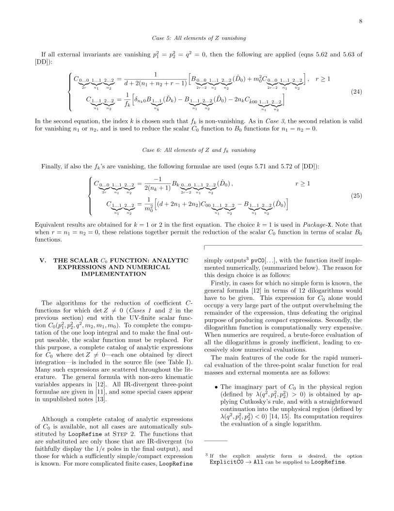
Case 5: All elements of Z vanishing

If all external invariants are vanishing p21 = p2

2 = q2 = 0, then the following are applied (eqns 5.62 and 5.63 of[DD]):

C 0...0︸︷︷︸2r

1...1︸︷︷︸n1

2...2︸︷︷︸n2

=1

d+ 2(n1 + n2 + r − 1)

[B 0...0︸︷︷︸

2r−2

1...1︸︷︷︸n1

2...2︸︷︷︸n2

(D0) +m20C 0...0︸︷︷︸

2r−2

1...1︸︷︷︸n1

2...2︸︷︷︸n2

], r ≥ 1

C 1...1︸︷︷︸n1

2...2︸︷︷︸n2

=1

fk

[δnk0B 1...1︸︷︷︸

nk

(Dk)−B 1...1︸︷︷︸n1

2...2︸︷︷︸n2

(D0)− 2nkCk00 1...1︸︷︷︸n1

2...2︸︷︷︸n2

] (24)

In the second equation, the index k is chosen such that fk is non-vanishing. As in Case 3, the second relation is validfor vanishing n1 or n2, and is used to reduce the scalar C0 function to B0 functions for n1 = n2 = 0.

Case 6: All elements of Z and fk vanishing

Finally, if also the fk’s are vanishing, the following formulae are used (eqns 5.71 and 5.72 of [DD]):C 0...0︸︷︷︸

2r

1...1︸︷︷︸n1

2...2︸︷︷︸n2

=−1

2(nk + 1)Bk 0...0︸︷︷︸

2r−2

1...1︸︷︷︸n1

2...2︸︷︷︸n2

(D0) , r ≥ 1

C 1...1︸︷︷︸n1

2...2︸︷︷︸n2

=1

m20

[(d+ 2n1 + 2n2)C00 1...1︸︷︷︸

n1

2...2︸︷︷︸n2

−B 1...1︸︷︷︸n1

2...2︸︷︷︸n2

(D0)] (25)

Equivalent results are obtained for k = 1 or 2 in the first equation. The choice k = 1 is used in Package-X. Note thatwhen r = n1 = n2 = 0, these relations together permit the reduction of the scalar C0 function in terms of scalar B0

functions.

V. THE SCALAR C0 FUNCTION: ANALYTICEXPRESSIONS AND NUMERICAL

IMPLEMENTATION

The algorithms for the reduction of coefficient C-functions for which detZ 6= 0 (Cases 1 and 2 in theprevious section) end with the UV-finite scalar func-tion C0(p2

1, p22, q

2,m2,m1,m0). To complete the compu-tation of the one loop integral and to make the final out-put useable, the scalar function must be replaced. Forthis purpose, a complete catalog of analytic expressionsfor C0 where detZ 6= 0—each one obtained by directintegration—is included in the source file (see Table I).Many such expressions are scattered throughout the lit-erature. The general formula with non-zero kinematicvariables appears in [12]. All IR-divergent three-pointformulae are given in [11], and some special cases appearin unpublished notes [13].

Although a complete catalog of analytic expressionsof C0 is available, not all cases are automatically sub-stituted by LoopRefine at Step 2. The functions thatare substituted are only those that are IR-divergent (tofaithfully display the 1/ε poles in the final output), andthose for which a sufficiently simple/compact expressionis known. For more complicated finite cases, LoopRefine

simply outputs3 pvC0[. . .], with the function itself imple-mented numerically, (summarized below). The reason forthis design choice is as follows:

Firstly, in cases for which no simple form is known, thegeneral formula [12] in terms of 12 dilogarithms wouldhave to be given. This expression for C0 alone wouldoccupy a very large part of the output overwhelming theremainder of the expression, thus defeating the originalpurpose of producing compact expressions. Secondly, thedilogarithm function is computationally very expensive.When numerics are required, a brute-force evaluation ofall the dilogarithms is grossly inefficient, leading to ex-cessively slow numerical evaluations.

The main features of the code for the rapid numeri-cal evaluation of the three-point scalar function for realmasses and external momenta are as follows:

• The imaginary part of C0 in the physical region(defined by λ(q2, p2

1, p22) > 0) is obtained by ap-

plying Cutkosky’s rule, and with a straightforwardcontinuation into the unphysical region (defined byλ(q2, p2

1, p22) < 0) [14, 15]. Its computation requires

the evaluation of a single logarithm.

3 If the explicit analytic form is desired, the optionExplicitC0→ All can be supplied to LoopRefine.

9

B-functions — Section IV A

B1...1(0; 0, 0) B1...1(p2; 0, 0) B1...1(m20;m0, 0) B1...1(p2;m0, 0)

B1...1(m20;m0,m0) B1...1(0;m0,m0) B1...1(0;m0,m1) B1...1((m0+m1)2;m0,m1)

B1...1(0; 0,m1) B1...1(m21; 0,m1) B1...1(p2; 0,m1) B1...1((m0−m1)2;m0,m1)

B1...1(0;m0, 0)

B-functions with r = −1 — Appendix E

B1...1(0; 0, 0) B1...1(p2; 0, 0) B1...1(m20;m0, 0) B1...1(p2;m0, 0)

B1...1(0; 0,m1) B1...1(0;m0,m0) B1...1(0;m0,m1) B1...1((m0+m1)2;m0,m1)B1...1(0;m0, 0) B1...1(m2

1; 0,m1) B1...1(p2; 0,m1) B1...1((m0−m1)2;m0,m1)

Auxiliary bξ-functions — Section IV B

bξ1...1(0, 0) bξ1...1(p2, 0)

bξ1...1(0,m) bξ1...1(m2,m)

Scalar C-functions — Section V

C0(0, 0, 0; 0, 0, 0) C0(0, 0, q2; 0,m0,m0) C0(m20, 0, q

2; 0, 0,m0) C0(0, p22, q2;m2, 0, 0)

C0(0, 0, q2; 0, 0, 0) C0(0, 0, q2; 0,m1,m0) C0(0,m22, q

2;m2, 0, 0) C0(p21, 0, q2;m2,m1,m0)

C0(0, 0,m22;m2, 0, 0) C0(0, 0, q2;m0,m0,m0) C0(m2

0, 0,m22;m2, 0,m0) C0(m2

0,m20, q

2; 0, 0,m0)C0(0, 0, q2;m2, 0, 0) C0(0, 0, q2;m2,m0,m0) C0(p21, p

22, q

2;m2,m1,m0) C0(m20, p

22,m

20;m0, 0,m0)

C0(0, 0, q2; 0, 0,m0) C0(0, 0, q2;m2,m1,m0) C0(0,m20, q

2; 0,m0,m0) C0(m20, p

22,m

22;m2, 0,m0)

C0(0, 0,m20;m0,m0,m0) C0(p21, 0, q

2; 0, 0, 0) C0(0, p22, q2;m0,m0,m0) C0(p21, p

22, q

2; 0, 0, 0)

TABLE I. Special kinematic cases of the Passarino-Veltman coefficient functions B, bξ and C for which explicit expressions areincluded in the source file OneLoop.m. Further information for these functions is found in the indicated sections

• The real part of C0 requires evaluations of onlythe real part (in the physical region) or only theimaginary part (in the unphysical region) of thedilogarithm, but not both. Calling PolyLog wouldlead to needless computation of both parts by theMathematica Kernel. Following [16], the real andimaginary parts of the dilogarithm function are im-plemented separately.

• For the real part of C0 in the physical region, the+iε prescription is irrelevant (since it influencesonly the imaginary part which is anyway evaluatedusing Cutkosky’s rule). Then, either the argumentsof the 12 dilogarithms come in complex-conjugatepairs (for which the real part of the dilogarithmsare identical and are added reducing the numberof dilog evaluations), or the arguments are purelyreal (for which the real parts of the dilogarithmsare rapidly evaluated using real arithmetic).

• The code is compiled to the Wolfram Virtual Ma-chine (using Compile), leading to a substantialboost in computation speed.

In the physical region, up to a 200-fold increase inspeed is achieved compared to brute-force Mathematicaevaluation by the Kernel. In the unphysical region, upto a 20-fold increase in speed is obtained. If the op-tion CompilationTarget→“C” to Compile is set, its per-formance rivals that of the Fortran implementation in

LoopTools, with Package-X generating results approx-imately twice as fast.

VI. HANDLING THE +iε PRESCRIPTION ANDSIMPLIFYING LOGARITHMS

The +iε prescription appearing in the denominatorsof propagator functions enforce causality in the time-ordered Green functions of a relativistic quantum fieldtheory. In one-loop computations, it determines thebranch on which the logarithms are to be evaluated. Alloutput expressions of LoopRefine observe the +iε pre-scription and are consistent with the analytic conventionsof the built-in Mathematica functions Log and PolyLog,which are

Log[x] −→ limε→0+

ln(x+ iε) , and

PolyLog[2, x] −→ limε→0+

Li2(x− iε) .

Because Package-X assumes real external invariants andinternal masses, almost all analytic formulae can be ex-pressed compactly in terms of the built-in functions.

Whenever LoopRefine generates a logarithm contain-ing the ratio of two internal masses, the ratio may beflipped to bring the logarithm to ‘canonical form’, e.g.

Log[m12m02

]−→ −Log

[m02m12

]. (26)

10

Since internal masses are assumed to be positive real,this is allowed, and helps to keep the logarithmic partscompact.

In the course of reduction, regardless of whether thefinal expression is divergent or finite, multiple logarithmsof ratios of several scales with the ’t Hooft parameter µ2

are typically generated, e.g.

a Log[µR2−s

]+ b Log

[µR2m2

]+ c Log

[ µR2

m2 − s

]. (27)

It is found that by consistently keeping µ2 in the numera-tor, the +iε prescription is always observed – even whenthe other scales are external invariants that may becometime-like. The µ2 from each logarithm are brought into asingle logarithm by forming the ratio with a variable thatis known to be positive (which were recorded at step 1):

(27) = a Log[ m2−s

]+ (a + b + c) Log

[µR2m2

]+ c Log

[ m2

m2 − s

]. (28)

That way, the coefficient—(a+b+c) in this example—ofthe µ2-dependent logarithm always matches that of the1/ε pole elsewhere in the expression, and are groupedbefore presenting the results. If the final expression werein fact finite without a 1/ε pole, the coefficient wouldcancel exactly.

In more complicated cases, expressions cannot be givencompactly assuming a universal sign for the infinitesi-mal imaginary part. In this case, Mathematica’s built-infunctions Log and PolyLog are unsuitable. For this pur-pose, two new analytic functions are defined in Package-X(within OneLoop‘):

Ln[x,a] −→ limε→0+

ln(x+ iaε) , and

DiLog[x,a] −→ limε→0+

Li2(x+ iaε) .

The (real part of the) second argument a controls the sideof the branch on which these functions evaluate. A simpleexample that uses DiLog in its output can be found byrunning

LoopRefine[pvC0[0, m2, s, 0, m, m]] .

VII. SPUR: COMPUTATION OF TRACES OFDIRAC MATRICES

To assist in the evaluation of one-loop integrals withinternal (closed) fermion lines, Package-X includes therudimentary function Spur (inside the module Spur‘) toevaluate traces over products of Dirac gamma matricesappearing in numerators. The function Projector helpsto handle loop integrals with open fermion lines and isdescribed in the next section. Because the primary func-tion of Package-X is to compute loop integrals, with the

computation of traces being a secondary feature, onlya cursory description of the algorithms are given in thefollowing two sections.

As with the rest of the algorithms in Package-X, thecalculation of traces is rule-based at its core, and bearssome resemblance to that of a much earlier Mathematicapackage Tracer[17]. However there are a number ofdifferences listed below that lead to greater computationspeed.

• Throughout the evaluation of the trace, expres-sions can grow very large containing many terms.Groups of terms are temporarily enclosed within aList to prevent the Mathematica kernel from au-tomatically simplifying the large expression at eachstep of the computation process.

• While more complicated trace formulae such asthose for products of numerous gamma matrices arerecursive, non-iterative rules are used for simplertasks such as for collecting γ5 and PL/PR withineach term.

• Products of gamma matrices with repeated Lorentzindices (such as γµγνγργµ) are related to productswith fewer gamma matrices. With more gammamatrices interposed between contracted matrices,the number of terms in the identity grows. Onaccount of the cyclic property of the trace, thesecontraction identities may be applied in one of twodirections. Additional rules are included so as toapply the identity in the direction with fewer num-ber of interposed gamma matrices.

• Traces that multiply γ5 are tagged differently toset it apart from those without it. This way, rulesfor computing traces with γ5 and those without γ5

are separated, and saves some time when the kernelsearches for the appropriate rules.

When compared to the other Mathematica packagesFeynCalc and Tracer, Package-X generally gives re-sults around 10 times faster. As an example, the trace

Tr[(/k − /p1

− /p2+m)γν(gLPL + gRPR)(/k − /p2

+m)

γρ(gLPL + gRPR)(/k +m)γµ(gLPL + gRPR)]

(29)

was calculated with each package and computation timeswere recorded (with Timing). The results on a 2.93 GHzIntel i7 processor are:

Package-X 0.096 sFeynCalc 8.2.0 1.03 sTracer 1.1 0.81 s

Part of the motivation for refining the trace-taking al-gorithms is due to the inclusion of fermion projectorsdescribed in the next section. When a Projector is in-cluded inside Spur, the number of terms within the traceis increased to an extent that a noticeable slowdown is ob-served. However, with the refinements described above,

11

projections onto form factors are nearly instantaneous ona modern computer.

VIII. PROJECTOR: PROJECTION ONTO FERMIONFORM FACTORS

Package-X does not directly handle expressions involv-ing open fermion chains that are relevant for fermion selfenergy and form factor calculations. In order to providesome support for such computations, Package-X comesequipped with a set of projectors. The projectors permitthe projection of a loop integral with an open fermionline onto specific form factors functions.

For example, the one-loop expression for the off-shellfermion self-energy function takes the form

I(/p) = µ2ε

∫ddk

(2π)dM(k, p)

[k2 −m2][(k + p)2], (30)

where M(k, p) is a Dirac matrix structure that dependson the integration variable k and external momentum p.Parity conservation and Lorentz covariance allow I to bewritten in the form

I(/p) = A(p2)/p+B(p2)m, (31)

where the form factors A and B depend on Lorentz in-variants p2 and m2 only. By multiplying the appropriateprojectors

F [A](p,m) =1

4p2 /p and F [B](p,m) =1

4m2

with the numerator of (30), and taking the trace, theform factors are obtained:

A(p2) = µ2ε

∫ddk

(2π)dTr[M(k, p)F [A](p,m)]

[k2 −m2][(k + p)2]

B(p2) = µ2ε

∫ddk

(2π)dTr[M(k, p)F [B](p,m)]

[k2 −m2][(k + p)2].

The trace over the projectors convert the expressions intoordinary tensors integrals that are readily computed withPackage-X.

A large set of pre-programmed projectors for off-shell self energy functions and on-shell scalar- andvector-vertex functions in various bases (L/R-chiral orVector/Axial-vector) are available (as Projector) tostreamline the computation of such integrals. These pro-jectors are generalizations of those used in [18] for the cal-culation of lepton anomalous magnetic moments, and in[19] for dipole moments. A comprehensive list of availableprojectors is given in the built-in documentation files.

IX. CROSSCHECKS AND FURTHERDEVELOPMENT

The verification of loop integrals obtained by Package-X is divided into two parts: checking the reduction algo-rithms in Section IV, and checking the basis functions in

Table I. The reduction routines for A and B coefficientfunctions and the basis B1...1 functions were comparedagainst another (unpublished) computer program devel-oped by Huaike Guo. The reduction of C functions forCases 1, 3, 5 and 6 were checked against explicit for-mulae for the low rank functions listed in [DD]. EachC0 scalar function was derived by hand and comparedagainst explicit formulae in the literature where they ex-ist [8, 11, 13, 20]. In cases where they did not exist,the analytic expressions were checked by comparing withthe results of numerically integrating the correspondingFeynman parameter representations given in AppendixB.

Finally, as a combined check of the various algorithmsin Package-X, the following well known physical quan-tities were computed and verified: H → gg and γγstandard model decay rates [21], electron g − 2, and theneutrino electric and magnetic moments [22]. Each wasfound to be in agreement with literature.

There are a number of important limitations of Pack-age-X, listed below, that guides its current line of devel-opment.

1. An analytic series expansion of the loop integral inkinematic variables is not generally possible. Cur-rently, the only available method is to use Math-ematica’s Series on the output of LoopRefine.However, if the result of loop integral contains spe-cially defined function like pvC0, then Series willnot work. Given that much information about aloop-integral can be gleaned from its expansion, theomission of this feature is most conspicuous.

2. Package-X currently supports loop integrals withup to only three denominator factors. But, as thenumber of denominator factors increases, so doesthe complexity of their analytic forms. Thus, itwould not be so practical to work with such ex-pressions for higher-point functions even if Pack-age-X were to provide them. However, at specialkinematic points such as at zero external momentaor at thresholds compact expressions could be ob-tained.

3. Gamma-5 is implemented naively in dimensionalregularization. This means that the VVA or AAAthree-point functions may not automatically satisfyWard identities appropriate to the physical prob-lem. However, the versatility of Package-X makesit easy to apply Adler’s method [23] (see also [24])to enforce the Ward identities.

4. Loop integrals with open fermion chains are notdirectly supported. As explained in Section VIII,there is no way to input an open string of Diracmatrices. Instead, the computation of fermion formfactors can be done by projecting out the neededform factors.

12

ACKNOWLEDGMENTS

I express my gratitude to the members of the Math-ematica StackExchange community for providing count-less answers to my questions regarding the technical as-pects of Mathematica and Wolfram Workbench. I thankAnsgar Denner for clarifying discussions regarding thereduction methods and for providing helpful informationregarding the literature. Numerous colleagues have pro-vided useful feedback: Huaike Guo for cross-checking sev-eral results during the early stages of the development,and Xunjie Xu for encouraging me to refine the trace-taking algorithms.

I also acknowledge my debt to beta tester JohannesWelter for cross-checking the fermion form factor projec-tors, and to beta testers Juri Smirnov and Michael Duerrfor identifying bugs. Special thanks goes to MichaelDuerr for meticulously hand-checking various results ofthe reduction algorithms, and for suggesting improve-ments to the user interface, the tutorial, and the accom-panying documentation pages.

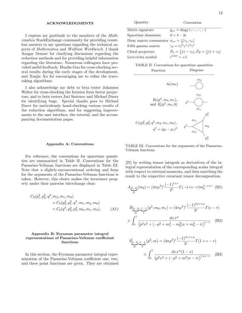
Appendix A: Conventions

For reference, the conventions for spacetime quanti-ties are summarized in Table II. Conventions for thePassarino-Veltman functions are displayed in Table III.Note that a slightly-unconventional ordering and formfor the arguments of the Passarino-Veltman functions istaken. However, this choice makes the invariance prop-erty under their pairwise interchange clear:

C0(p21, p

22, q

2,m2,m1,m0)

= C0(p22, p

21, q

2,m1,m2,m0)

= C0(q2, p22, p

21,m0,m1,m2) . (A1)

Appendix B: Feynman parameter integralrepresentations of Passarino-Veltman coefficient

functions

In this section, the Feynman parameter integral repre-sentation of the Passarino-Veltman coefficient one, two,and three point functions are given. They are obtained

Quantity Convention

Metric signature gµν = diag(+,−,−,−)

Spacetime dimension d = 4− 2ε

Dirac matrix commutator σµν = i2[γµ, γν ]

Fifth gamma matrix γ5 = iγ0γ1γ2γ3

Chiral projectors PL = 12(1− γ5), PR = 1

2(1 + γ5)

Levi-civita symbol ε0123 = +1

TABLE II. Conventions for spacetime quantities

Function Diagram

A0(m0)m0

B0(p2,m0,m1),

and bξ0(p2,m0, 0)

m0

m1

p2

C0(p21, p22, q

2,m2,m1,m0) ,

q2 = (p2 − p1)2m2

m0

m1

q2

p22

p21

TABLE III. Conventions for the arguments of the Passarino-Veltman functions

[25] by writing tensor integrals as derivatives of the in-tegral representation of the corresponding scalar integralwith respect to external momenta, and then matching theresult to the respective covariant tensor decomposition.

A 0...0︸︷︷︸2r

(m0) = (4πµ2)ε(−1)1+r

2rΓ(−1+ε−r)m1−ε+r

0 (B1)

B 0...0︸︷︷︸2r

1...1︸︷︷︸n

(p2;m0,m1) = (4πµ2)ε(−1)2+r+n

2rΓ(ε− r)

×∫ 1

0

dxxn(p2x2 + (−p2 +m2

1 −m20)x+m2

0 − iε)ε−r (B2)

bξ0...0︸︷︷︸2r

1...1︸︷︷︸n

(p2;m) = (4πµ2)ε(−1)3+r+n

2rΓ(1 + ε− r)

×∫ 1

0

dxxn(1− x)(p2x2 + (−p2 +m2)x− iε

)1+ε−r (B3)

13

C 0...0︸︷︷︸2r

1...1︸︷︷︸n1

2...2︸︷︷︸n2

(p21, p

22, q

2;m2,m1,m0) = (4πµ2)ε(−1)3+r+n1+n2

2rΓ(1 + ε− r)

×∫ 1

0

dy

∫ 1−y

0

dz yn1zn2[p2

1y2 +p2

2z2 + (−q2 +p2

1 +p22)yz+ (−p2

1 +m21−m2

0)y+ (−p22 +m2

2−m20)z+m2

0− iε]−1−ε+r

(B4)

The coefficient C function exhibits an invariance under the simultaneous interchange of indices n1 ↔ n2, externalmomenta p2

1 ↔ p22 and internal masses m1 ↔ m2,

C 0...0︸︷︷︸2r

1...1︸︷︷︸n1

2...2︸︷︷︸n2

(p21, p

22, q

2;m2,m1,m0) = C 0...0︸︷︷︸2r

1...1︸︷︷︸n2

2...2︸︷︷︸n1

(p22, p

21, q

2;m1,m2,m0) (B5)

and is frequently employed during its reduction in the most general kinematic case (detZ 6= 0).In certain reduction formulae of C-functions, some terms are multiplied by ε, which in the ε → 0 limit, pick up

the UV-divergent parts of the coefficient functions in those terms. The UV divergent parts are readily obtained fromthe integral representation. They are controlled by the leading gamma function which for large enough r develops a1/ε pole as ε → 0. When r is large, the integrand becomes polynomial in the Feynman parameters and are readilyintegrated with the help of the multinomial theorem. The needed UV-divergent parts are those of the B and Cfunctions, shown below.

B 0...0︸︷︷︸2r

1...1︸︷︷︸n

(p2;m0,m1)∣∣∣UV-Div.

=(−1)n

2rr!

∑k1+k2+k3=r

(r

k1, k2, k3

)ak1bk2ck3

2k1 + k2 + n+ 1

1

ε, (B6)

where a = p2, b = −p2 +m21 −m2

0, and c = m20, are polynomial coefficients of the integrand in (B2).

C 0...0︸︷︷︸2r

1...1︸︷︷︸n1

2...2︸︷︷︸n2

(p21, p

22, q

2;m2,m1,m0)∣∣∣UV-Div.

=(−1)n1+n2

2r(r − 1)!

∑k1+...+k6=r−1

(r − 1

k1, . . . , k6

)ak1bk2ck3dk4ek5fk6

(2k1 + k3 + k4 + n1)!(2k2 + k3 + k5 + n2)!

(2k1 + 2k2 + 2k3 + k4 + k5 + n1 + n2 + 2)!

1

ε, (B7)

where a, b, c, d, e, and f are polynomial coefficients of the integrand in (B4) in the order displayed.

Appendix C: Derivation of reduction formulae for C functions Case 2

The derivation of the first equation in (19) begins with the Feynman parameter representation of the coefficient Cfunction,

C 0...0︸︷︷︸2r

1...1︸︷︷︸n1

2...2︸︷︷︸n2

(m20, s,m

22;m2, 0,m0) = (4πµ2)ε

(−1)3+r+n1+n2

2rΓ(1 + ε− r)

×∫ 1

0

dy

∫ 1−y

0

dz yn1zn2[m2

0y2 + sz2 + (−m2

2 +m20 + s)yz + (−m2

0 +m22 − s)z +m2

0 − iε]−1−ε+r

. (C1)

Upon making a change of integration variables y = 1− y′ and z = y′z′, the nested integrals are factored:

integrals =

∫ 1

0

dy′ y′−1+n2−2ε+2r(1− y′)n1

∫ 1

0

dz′ z′n2[sz′2 + (−s+m2

2 −m20)z′ +m2

0 − iε]−1−ε+r

. (C2)

The y′ integral gives the Euler Beta function, while the z′ integral is identified as the integral representation ofcoefficient B-function (B2).

C 0...0︸︷︷︸2r

1...1︸︷︷︸n1

2...2︸︷︷︸n2

(m20, s,m

22;m2, 0,m0) =

(−1)n1

2B(n2 − 2ε+ 2r, n1 + 1)B 0...0︸︷︷︸

2r−2

1...1︸︷︷︸n2

(s;m0,m2) (C3)

14

As long as one of n2 or r is non-zero, the Beta function is finite, and its expansion to O(ε) may be inserted yieldingthe first equation in (19).

On the other hand, if n2 = r = 0, the Beta function develops a 1/ε pole, so that to O(ε),

B(−2ε, n1 + 1) = −12ε −Hn1 − ε

(H2n1−H(2)

n1

). In this case, (C1) is written as

C 1...1︸︷︷︸n1

(m20, s,m

22;m2, 0,m0) = (4πµ2)ε(−1)n1Γ(1 + ε)

1

2ε

∫ 1

0

dz′(sz′2 + z′(−s+m2

2 −m20) +m2

0 − iε)−1−ε

+ (4πµ2)ε(−1)n1Γ(1 + ε)(Hn1

+ ε(H2n1−H(2)

n1)) ∫ 1

0

dz′(sz′2 + z′(−s+m2

2 −m20) +m2

0 − iε)−1−ε

. (C4)

While the z′ integral in the second line can be identified with the integral representation of the coefficient B function,the first line is identified4 as the integral representation of the scalar function C0(m2

0, s,m22;m2, 0,m0) classified by

Ellis and Zanderighi [11] as IR-divergent triangle 6. These identifications lead to the second equation of (19).If the off-shell momentum s is in the third argument, the derivation starts with the change of variables z = 1−y−x

in (B4) followed by an interchange of the x and y integrals to give

C 0...0︸︷︷︸2r

1...1︸︷︷︸n1

2...2︸︷︷︸n2

(m22,m

20, s;m0,m2, 0) = (4πµ2)ε

(−1)3+r+n1+n2

2rΓ(1 + ε− r)

×∫ 1

0

dx

∫ 1−x

0

dy yn1(1− x− y)n2[m2

0x2 + sy2 + (s+m2

0 −m22)xy − 2m2

0x+ (−s−m20 +m2

2)y +m20 − iε

]−1−ε+r.

(C5)

The nested integrals are factored by making a further change of variables x = 1− x′ and y = y′x′ to give

integrals =

∫ 1

0

dx′ x′n1+n2+2r−1−2ε

∫ 1

0

dy′ y′n1(1− y′)n2[sy′2 + (−s+m2

2 −m20)y′ +m2

0 − iε]−1−ε+r

. (C6)

The x′ integral is straightforward. The y′ integral can be brought to a recognizable form after expanding the factor(1− y′)n2 as a binomial series

=1

n1 + n2 + 2r − 2ε

n2∑k=0

(n2

k

)(−1)k

∫ 1

0

dy′ y′n1+k[sy′2 + (−s+m2

2 −m20)y′ +m2

0 − iε]−1−ε+r

. (C7)

The y′ integral is now identified as the integral representation of the coefficient B function, yielding (20).

Appendix D: Derivation of reduction formulae for C functions Case 4

Two cases are distinguished for Case 4 (detZ = 0, X0j = 0) depending on whether p22 is vanishing. Although

the steps below leading to (22) and (23) appear complicated, they essentially follow that of [12] for the evaluation ofthe scalar function C0. Beginning with the integral representation (B4), a change of integration variables y = 1− y′brings the Feynman integrals to the form

integrals =

∫ 1

0

dy′∫ y′

0

dz (1− y′)n1zn2[a y′2 + b z2 + c y′z + d y′ + e z + f

]−1−ε+r(D1)

where a = p21, b = p2

2, c = q2 − p21 − p2

2, d = −p21 +m2

0 −m21, e = p2

1 − q2 −m20 +m2

2, and f = m21 − iε.

Under the assumption that p22 6= 0, a second change of variables is made z = z′ +αy′, with α = −c

2b chosen to make

the coefficient of y′2 in square brackets vanish.

integrals =

∫ 1

0

dy′∫ (1−α)y

−αydz′ (1− y′)n1(z′ + αy′)n2

[bz′2 + (c+ 2bα)y′z′ + (d+ eα)y′ + e z′ + f

]−1−ε+r(D2)

4 see http://qcdloop.fnal.gov/tridiv6.pdf

15

The choice for α implies that c + 2bα vanishes, and the kinematic relations detZ = X0j = 0 imply that d + eαvanishes, yielding

integrals =

∫ 1

0

dy

∫ (1−α)y

−αydz (1− y)n1(z + αy)n2

[bz2 + e z + f

]−1−ε+r, (D3)

where the primes have been omitted. The binomial theorem is applied to the factor (z+αy)n2 =∑j

(n2

j

)αn2−jyn2−jzj ,

and the order of integrations is interchanged so that

integrals =

n2∑j=0

(n2

j

)αn2−j

[ ∫ 1−α

0

dz

∫ 1

z/(1−α)

dy −∫ −α

0

dz

∫ 1

−z/αdy](1− y)n1yn2−jzj

[bz2 + e z + f

]−1−ε+r. (D4)

The y integrals in both terms yield terminating hypergeometric series most compactly written in terms of the incom-plete Beta function: ∫ 1

X

dy(1− y)n1yn2−j =n1!(n2 − j)!

(n1 + n2 − j + 1)!− BX(n2 − j + 1, n1 + 1)

=n1!(n2 − j)!

(n1 + n2 − j + 1)!−

n1∑k=0

(−1)kXn2−j+k+1

(n2 − j + k + 1)

(n1

k

). (D5)

Since the first term of (D5) is common to both integrations in (D4), they are combined to yield a total of three terms:

integrals =

n2∑j=0

(n2

j

)αn2−j

[ n1!(n2 − j)!(n1 + n2 − j + 1)!

∫ 1−α

−αdz

zn2+j

(bz2 + ez + f)1+ε−r

−∫ 1−α

0

dzBz/(1−α)(n2 − j + 1, n1 + 1) zj

(bz2 + ez + f)1+ε−r +

∫ −α0

dzB−z/α(n2 − j + 1, n1 + 1) zj

(bz2 + ez + f)1+ε−r

](D6)

A change of integration variables is carried out in each term to stretch their ranges to 0 → 1: In the first integral,z = z′ − α, in the second integral z = (1 − α)z′, and in the third integral z = −αz′. Consequently, the polynomialsbz2 + ez + f take the shape of integrands for the B functions5:

First term: p22z′2 + (−p2

2 +m22 −m2

0)z′ +m20 − iε := P2(z′)

Second term: q2z′2 + (−q2 +m22 −m2

1)z′ +m21 − iε := P12(z′)

Third term: p21z′2 + (−p2

1 +m20 −m2

1)z′ +m21 − iε := P1(z′)

Upon inserting the series representation of the incomplete Beta function (D5) the result is (after dropping the primeson z)

integrals =

n2∑j=0

(n2

j

)αn2−j

{n1!(n2 − j)!

(n1 + n2 − j + 1)!

∫ 1

0

dz(z − α)jP2(z)−1−ε+r

+

n1∑k=0

(−1)k

n2 − j + k + 1

(n1

k

)[− (1− α)j+1

∫ 1

0

dz zn2+k+1P12(z)−1−ε+r + (−α)j+1

∫ 1

0

dz zn2+k+1P1(z)−1−ε+r]}(D7)

In the first term, the binomial theorem is applied to (z−α)j =∑k

(jk

)(−α)j−kzk, and the three z integrals are finally

identified as integral representations of the coefficient B functions upon which (22) is obtained.If p2

2 = 0, equation (22) breaks down and another formulae is needed. In this case, detZ = 0 implies p21 = q2 and

X0j = 0 implies m0 = m2 provided p21 6= 0. With these relations, the integrals in (D1) are already factored:

integrals =

∫ 1

0

dy′∫ y′

0

dz (1− y′)n1zn2[p2

1y′2 + (−p2

1 +m20 −m2

1)y′ +m21 − iε

]−1−ε+r. (D8)

5 These quadratic polynomials may be recognized as the ‘pinchfunctions’ originating from the three cut channels of the triangle

graph.

16

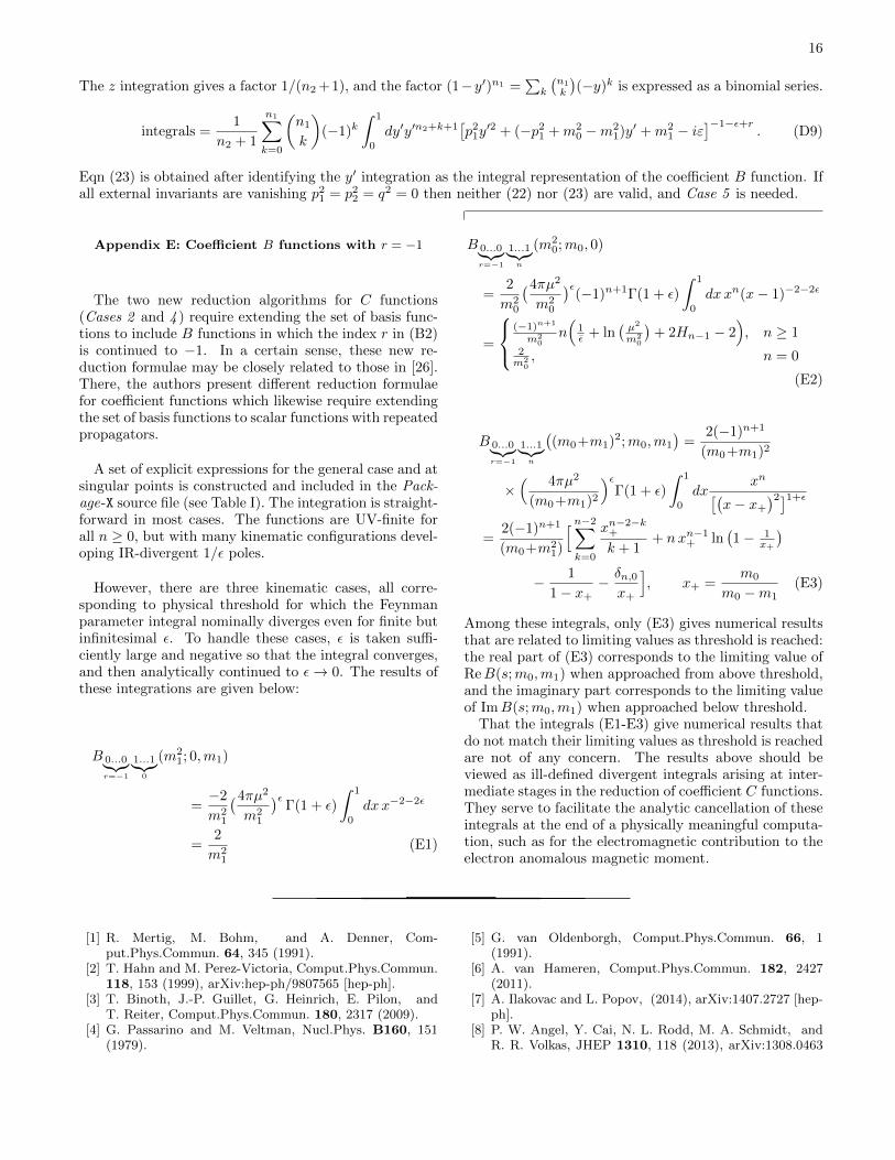
The z integration gives a factor 1/(n2 +1), and the factor (1−y′)n1 =∑k

(n1

k

)(−y)k is expressed as a binomial series.

integrals =1

n2 + 1

n1∑k=0

(n1

k

)(−1)k

∫ 1

0

dy′y′n2+k+1[p2

1y′2 + (−p2

1 +m20 −m2

1)y′ +m21 − iε

]−1−ε+r. (D9)

Eqn (23) is obtained after identifying the y′ integration as the integral representation of the coefficient B function. Ifall external invariants are vanishing p2

1 = p22 = q2 = 0 then neither (22) nor (23) are valid, and Case 5 is needed.

Appendix E: Coefficient B functions with r = −1

The two new reduction algorithms for C functions(Cases 2 and 4 ) require extending the set of basis func-tions to include B functions in which the index r in (B2)is continued to −1. In a certain sense, these new re-duction formulae may be closely related to those in [26].There, the authors present different reduction formulaefor coefficient functions which likewise require extendingthe set of basis functions to scalar functions with repeatedpropagators.

A set of explicit expressions for the general case and atsingular points is constructed and included in the Pack-age-X source file (see Table I). The integration is straight-forward in most cases. The functions are UV-finite forall n ≥ 0, but with many kinematic configurations devel-oping IR-divergent 1/ε poles.

However, there are three kinematic cases, all corre-sponding to physical threshold for which the Feynmanparameter integral nominally diverges even for finite butinfinitesimal ε. To handle these cases, ε is taken suffi-ciently large and negative so that the integral converges,and then analytically continued to ε→ 0. The results ofthese integrations are given below:

B 0...0︸︷︷︸r=−1

1...1︸︷︷︸0

(m21; 0,m1)

=−2

m21

(4πµ2

m21

)εΓ(1 + ε)

∫ 1

0

dxx−2−2ε

=2

m21

(E1)

B 0...0︸︷︷︸r=−1

1...1︸︷︷︸n

(m20;m0, 0)

=2

m20

(4πµ2

m20

)ε(−1)n+1Γ(1 + ε)

∫ 1

0

dxxn(x− 1)−2−2ε

=

(−1)n+1

m20

n(

1ε + ln

(µ2

m20

)+ 2Hn−1 − 2

), n ≥ 1

2m2

0, n = 0

(E2)

B 0...0︸︷︷︸r=−1

1...1︸︷︷︸n

((m0+m1)2;m0,m1

)=

2(−1)n+1

(m0+m1)2

×( 4πµ2

(m0+m1)2

)εΓ(1 + ε)

∫ 1

0

dxxn[(

x− x+

)2]1+ε

=2(−1)n+1

(m0+m21)

[ n−2∑k=0

xn−2−k+

k + 1+ nxn−1

+ ln(1− 1

x+

)− 1

1− x+− δn,0

x+

], x+ =

m0

m0 −m1(E3)

Among these integrals, only (E3) gives numerical resultsthat are related to limiting values as threshold is reached:the real part of (E3) corresponds to the limiting value ofReB(s;m0,m1) when approached from above threshold,and the imaginary part corresponds to the limiting valueof ImB(s;m0,m1) when approached below threshold.

That the integrals (E1-E3) give numerical results thatdo not match their limiting values as threshold is reachedare not of any concern. The results above should beviewed as ill-defined divergent integrals arising at inter-mediate stages in the reduction of coefficient C functions.They serve to facilitate the analytic cancellation of theseintegrals at the end of a physically meaningful computa-tion, such as for the electromagnetic contribution to theelectron anomalous magnetic moment.

[1] R. Mertig, M. Bohm, and A. Denner, Com-put.Phys.Commun. 64, 345 (1991).

[2] T. Hahn and M. Perez-Victoria, Comput.Phys.Commun.118, 153 (1999), arXiv:hep-ph/9807565 [hep-ph].

[3] T. Binoth, J.-P. Guillet, G. Heinrich, E. Pilon, andT. Reiter, Comput.Phys.Commun. 180, 2317 (2009).

[4] G. Passarino and M. Veltman, Nucl.Phys. B160, 151(1979).

[5] G. van Oldenborgh, Comput.Phys.Commun. 66, 1(1991).

[6] A. van Hameren, Comput.Phys.Commun. 182, 2427(2011).

[7] A. Ilakovac and L. Popov, (2014), arXiv:1407.2727 [hep-ph].

[8] P. W. Angel, Y. Cai, N. L. Rodd, M. A. Schmidt, andR. R. Volkas, JHEP 1310, 118 (2013), arXiv:1308.0463

17

[hep-ph].[9] A. Denner and S. Dittmaier, Nucl.Phys. B734, 62 (2006),

arXiv:hep-ph/0509141 [hep-ph].[10] D. Y. Bardin and G. Passarino, The standard model in the

making: Precision study of the electroweak interactions(Oxford Science Publications, 1999).

[11] R. K. Ellis and G. Zanderighi, JHEP 0802, 002 (2008),arXiv:0712.1851 [hep-ph].

[12] G. ’t Hooft and M. Veltman, Nucl.Phys. B153, 365(1979).

[13] J. C. Romao, “Modern Techniques for One-Loop Calcula-tions,” (2006), http://porthos.ist.utl.pt/OneLoop/one-loop.pdf.

[14] C. Fronsdal and R. E. Norton, J.Math.Phys 5, 100(1964).

[15] W. Lucha, D. Melikhov, and S. Simula, Phys.Rev. D75,016001 (2007), arXiv:hep-ph/0610330 [hep-ph].

[16] C. Osacar, J. Palacian, and M. Palacios, Celes. Mech.Dyn. Astro. 62, 93 (1995).

[17] M. Jamin and M. E. Lautenbacher, Com-put.Phys.Commun. 74, 265 (1993).

[18] E. R. R. Roskies, M. Levine, Quantum Electrodynamics,edited by T. Kinoshita, pp. 162–217 (World Scientific,Singapore, 1990).

[19] A. Czarnecki and B. Krause, Acta Phys.Polon. B28, 829(1997), arXiv:hep-ph/9611299 [hep-ph].

[20] L. G. Cabral-Rosetti and M. A. Sanchis-Lozano,J.Phys.Conf.Ser. 37, 82 (2006), arXiv:hep-ph/0206081[hep-ph].

[21] A. Djouadi, Phys.Rept. 457, 1 (2008).[22] C. Giunti and A. Studenikin, (2014), arXiv:1403.6344

[hep-ph].[23] S. L. Adler, Lectures on Elementary Particles and Quan-

tum Field Theory, edited by H. P. S. Deser, M. Grisaru,Vol. 1 (M.I.T. Press, Cambridge, 1970).

[24] F. Jegerlehner, Eur.Phys.J. C18, 673 (2001).[25] A. I. Davydychev, Phys.Lett. B263, 107 (1991).[26] G. Duplancic and B. Nizic, Eur.Phys.J. C35, 105 (2004).