Package ‘rockchalk’ - The Comprehensive R Archive … · Package ‘rockchalk’ May 14, 2018...
114
Package ‘rockchalk’ May 14, 2018 Type Package Title Regression Estimation and Presentation Version 1.8.111 Date 2018-05-14 Author Paul E. Johnson <[email protected]> Maintainer Paul E. Johnson <[email protected]> Description A collection of functions for interpretation and presentation of regression analysis. These functions are used to produce the statistics lectures in <http://pj.freefaculty.org/guides>. Includes regression diagnostics, regression tables, and plots of interactions and ``moderator'' variables. The emphasis is on ``mean-centered'' and ``residual-centered'' predictors. The vignette 'rockchalk' offers a fairly comprehensive overview. The vignette 'Rstyle' has advice about coding in R. The package title 'rockchalk' refers to our school motto, 'Rock Chalk Jayhawk, Go K.U.'. License GPL (>= 3.0) LazyLoad yes Imports grDevices, methods, lme4, car, MASS Suggests tables, Hmisc RoxygenNote 6.0.1 NeedsCompilation no Depends R (>= 2.10) Repository CRAN Date/Publication 2018-05-14 15:49:46 UTC R topics documented: rockchalk-package ..................................... 3 addLines ........................................... 4 centerNumerics ....................................... 5 1
-
Upload
nguyencong -
Category
Documents
-
view
243 -
download
0
Transcript of Package ‘rockchalk’ - The Comprehensive R Archive … · Package ‘rockchalk’ May 14, 2018...
Package ‘rockchalk’May 14, 2018
Type Package
Title Regression Estimation and Presentation
Version 1.8.111
Date 2018-05-14
Author Paul E. Johnson <[email protected]>
Maintainer Paul E. Johnson <[email protected]>
Description A collection of functions for interpretation and presentationof regression analysis. These functions are usedto produce the statistics lectures in<http://pj.freefaculty.org/guides>. Includes regressiondiagnostics, regression tables, and plots of interactions and``moderator'' variables. The emphasis is on ``mean-centered'' and``residual-centered'' predictors. The vignette 'rockchalk' offers afairly comprehensive overview. The vignette 'Rstyle' has adviceabout coding in R. The package title 'rockchalk' refers to ourschool motto, 'Rock Chalk Jayhawk, Go K.U.'.
License GPL (>= 3.0)
LazyLoad yes
Imports grDevices, methods, lme4, car, MASS
Suggests tables, Hmisc
RoxygenNote 6.0.1
NeedsCompilation no
Depends R (>= 2.10)
Repository CRAN
Date/Publication 2018-05-14 15:49:46 UTC
R topics documented:rockchalk-package . . . . . . . . . . . . . . . . . . . . . . . . . . . . . . . . . . . . . 3addLines . . . . . . . . . . . . . . . . . . . . . . . . . . . . . . . . . . . . . . . . . . . 4centerNumerics . . . . . . . . . . . . . . . . . . . . . . . . . . . . . . . . . . . . . . . 5
1
2 R topics documented:
centralValues . . . . . . . . . . . . . . . . . . . . . . . . . . . . . . . . . . . . . . . . 7cheating . . . . . . . . . . . . . . . . . . . . . . . . . . . . . . . . . . . . . . . . . . . 7checkIntFormat . . . . . . . . . . . . . . . . . . . . . . . . . . . . . . . . . . . . . . . 9checkPosDef . . . . . . . . . . . . . . . . . . . . . . . . . . . . . . . . . . . . . . . . 9combineLevels . . . . . . . . . . . . . . . . . . . . . . . . . . . . . . . . . . . . . . . 10cutByQuantile . . . . . . . . . . . . . . . . . . . . . . . . . . . . . . . . . . . . . . . . 11cutBySD . . . . . . . . . . . . . . . . . . . . . . . . . . . . . . . . . . . . . . . . . . . 12cutByTable . . . . . . . . . . . . . . . . . . . . . . . . . . . . . . . . . . . . . . . . . 13dir.create.unique . . . . . . . . . . . . . . . . . . . . . . . . . . . . . . . . . . . . . . . 13focalVals . . . . . . . . . . . . . . . . . . . . . . . . . . . . . . . . . . . . . . . . . . 14formatNumericSummaries . . . . . . . . . . . . . . . . . . . . . . . . . . . . . . . . . 15genCorrelatedData . . . . . . . . . . . . . . . . . . . . . . . . . . . . . . . . . . . . . 16genCorrelatedData2 . . . . . . . . . . . . . . . . . . . . . . . . . . . . . . . . . . . . . 17genX . . . . . . . . . . . . . . . . . . . . . . . . . . . . . . . . . . . . . . . . . . . . . 20getAuxRsq . . . . . . . . . . . . . . . . . . . . . . . . . . . . . . . . . . . . . . . . . 22getDeltaRsquare . . . . . . . . . . . . . . . . . . . . . . . . . . . . . . . . . . . . . . . 22getFocal . . . . . . . . . . . . . . . . . . . . . . . . . . . . . . . . . . . . . . . . . . . 23getPartialCor . . . . . . . . . . . . . . . . . . . . . . . . . . . . . . . . . . . . . . . . 25getVIF . . . . . . . . . . . . . . . . . . . . . . . . . . . . . . . . . . . . . . . . . . . . 26kurtosis . . . . . . . . . . . . . . . . . . . . . . . . . . . . . . . . . . . . . . . . . . . 27lazyCor . . . . . . . . . . . . . . . . . . . . . . . . . . . . . . . . . . . . . . . . . . . 28lazyCov . . . . . . . . . . . . . . . . . . . . . . . . . . . . . . . . . . . . . . . . . . . 29lmAuxiliary . . . . . . . . . . . . . . . . . . . . . . . . . . . . . . . . . . . . . . . . . 30magRange . . . . . . . . . . . . . . . . . . . . . . . . . . . . . . . . . . . . . . . . . . 30makeSymmetric . . . . . . . . . . . . . . . . . . . . . . . . . . . . . . . . . . . . . . . 31makeVec . . . . . . . . . . . . . . . . . . . . . . . . . . . . . . . . . . . . . . . . . . . 32mcDiagnose . . . . . . . . . . . . . . . . . . . . . . . . . . . . . . . . . . . . . . . . . 33mcGraph1 . . . . . . . . . . . . . . . . . . . . . . . . . . . . . . . . . . . . . . . . . . 34meanCenter . . . . . . . . . . . . . . . . . . . . . . . . . . . . . . . . . . . . . . . . . 36model.data . . . . . . . . . . . . . . . . . . . . . . . . . . . . . . . . . . . . . . . . . . 40model.data.default . . . . . . . . . . . . . . . . . . . . . . . . . . . . . . . . . . . . . . 41mvrnorm . . . . . . . . . . . . . . . . . . . . . . . . . . . . . . . . . . . . . . . . . . 44newdata . . . . . . . . . . . . . . . . . . . . . . . . . . . . . . . . . . . . . . . . . . . 46outreg . . . . . . . . . . . . . . . . . . . . . . . . . . . . . . . . . . . . . . . . . . . . 53outreg0 . . . . . . . . . . . . . . . . . . . . . . . . . . . . . . . . . . . . . . . . . . . 58outreg2HTML . . . . . . . . . . . . . . . . . . . . . . . . . . . . . . . . . . . . . . . . 62padW0 . . . . . . . . . . . . . . . . . . . . . . . . . . . . . . . . . . . . . . . . . . . . 63pctable . . . . . . . . . . . . . . . . . . . . . . . . . . . . . . . . . . . . . . . . . . . . 64perspEmpty . . . . . . . . . . . . . . . . . . . . . . . . . . . . . . . . . . . . . . . . . 66plot.testSlopes . . . . . . . . . . . . . . . . . . . . . . . . . . . . . . . . . . . . . . . . 68plotCurves . . . . . . . . . . . . . . . . . . . . . . . . . . . . . . . . . . . . . . . . . . 68plotFancy . . . . . . . . . . . . . . . . . . . . . . . . . . . . . . . . . . . . . . . . . . 73plotPlane . . . . . . . . . . . . . . . . . . . . . . . . . . . . . . . . . . . . . . . . . . 74plotSeq . . . . . . . . . . . . . . . . . . . . . . . . . . . . . . . . . . . . . . . . . . . 79plotSlopes . . . . . . . . . . . . . . . . . . . . . . . . . . . . . . . . . . . . . . . . . . 80predictCI . . . . . . . . . . . . . . . . . . . . . . . . . . . . . . . . . . . . . . . . . . 85predictOMatic . . . . . . . . . . . . . . . . . . . . . . . . . . . . . . . . . . . . . . . . 86print.factorSummaries . . . . . . . . . . . . . . . . . . . . . . . . . . . . . . . . . . . 93
rockchalk-package 3
print.pctable . . . . . . . . . . . . . . . . . . . . . . . . . . . . . . . . . . . . . . . . . 93print.summarize . . . . . . . . . . . . . . . . . . . . . . . . . . . . . . . . . . . . . . . 94print.summary.pctable . . . . . . . . . . . . . . . . . . . . . . . . . . . . . . . . . . . . 95religioncrime . . . . . . . . . . . . . . . . . . . . . . . . . . . . . . . . . . . . . . . . 95residualCenter . . . . . . . . . . . . . . . . . . . . . . . . . . . . . . . . . . . . . . . . 96skewness . . . . . . . . . . . . . . . . . . . . . . . . . . . . . . . . . . . . . . . . . . 99standardize . . . . . . . . . . . . . . . . . . . . . . . . . . . . . . . . . . . . . . . . . 100summarize . . . . . . . . . . . . . . . . . . . . . . . . . . . . . . . . . . . . . . . . . . 101summarizeFactors . . . . . . . . . . . . . . . . . . . . . . . . . . . . . . . . . . . . . . 104summarizeNumerics . . . . . . . . . . . . . . . . . . . . . . . . . . . . . . . . . . . . 106summary.factor . . . . . . . . . . . . . . . . . . . . . . . . . . . . . . . . . . . . . . . 107summary.pctable . . . . . . . . . . . . . . . . . . . . . . . . . . . . . . . . . . . . . . 108testSlopes . . . . . . . . . . . . . . . . . . . . . . . . . . . . . . . . . . . . . . . . . . 108vech2Corr . . . . . . . . . . . . . . . . . . . . . . . . . . . . . . . . . . . . . . . . . . 110vech2mat . . . . . . . . . . . . . . . . . . . . . . . . . . . . . . . . . . . . . . . . . . 111
Index 113
rockchalk-package rockchalk: regression functions
Description
Includes an ever-growing collection of functions that assist in the presentation of regression mod-els. The initial function was outreg, which produces LaTeX tables that summarize one or manyfitted regression models. It also offers plotting conveniences like plotPlane and plotSlopes,which illustrate some of the variables from a fitted regression model. For a detailed check on multi-collinearity, see mcDiagnose. The user should be aware of this fact: Not all of these functions leadto models or types of analysis that we endorese. Rather, they all lead to analysis that is endorsedby some scholars, and we feel it is important to facilitate the comparison of competing methods.For example, the function standardize will calculate standardized regression coefficients for allpredictors in a regression model’s design matrix in order to replicate results from other statisticalframeworks, no matter how unwise the use of such coefficients might be. The function meanCenterwill allow the user to more selectively choose variables for centering (and possibly standardization)before they are entered into the design matrix. Because of the importance of interaction variables inregression analysis, the residualCenter and meanCenter functions are offered. While mean cen-tering does not actually help with multicollinearity of interactive terms, many scholars have arguedthat it does. The meanCenter function can be compared with the "residual centering" of interactionterms.
Author(s)
Paul E. Johnson <[email protected]>
References
http://pj.freefaculty.org/R
4 addLines
addLines Superimpose regression lines on a plotted plane
Description
The examples will demonstrate the intended usage.
Usage
addLines(to = NULL, from = NULL, col, lwd = 2, lty = 1)
Arguments
to a 3d plot object produced by plotPlane
from output from a plotSlopes or plotCurves function (class="rockchalk")
col color of plotted lines (default: "red")
lwd line width of added lines (default: 2)
lty line type of added lines (default: 1)
Details
From an educational stand point, the objective is to assist with the student’s conceptualization ofthe two and three dimensional regression relationships.
Value
NULL, nothing, nicht, nada.
Author(s)
Paul E. Johnson <[email protected]>
Examples
##library(rockchalk)
set.seed(12345)
dfadd <- genCorrelatedData2(100, means = c(0,0,0,0), sds = 1, rho = 0,beta = c(0.03, 0.01, 0.1, 0.4, -0.1), stde = 2)
dfadd$xcat1 <- gl(2,50, labels=c("M","F"))
dfadd$xcat2 <- cut(rnorm(100), breaks=c(-Inf, 0, 0.4, 0.9, 1, Inf),labels=c("R", "M", "D", "P", "G"))
dfadd$y2 <- 0.03 + 0.1*dfadd$x1 + 0.1*dfadd$x2 +
centerNumerics 5
0.25*dfadd$x1*dfadd$x2 + 0.4*dfadd$x3 - 0.1*dfadd$x4 +0.2 * as.numeric(dfadd$xcat1) +contrasts(dfadd$xcat2)[as.numeric(dfadd$xcat2), ] %*% c(-0.1, 0.1, 0.2, 0) +1 * rnorm(100)
summarize(dfadd)
## linear ordinary regressionm1 <- lm(y ~ x1 + x2 + x3 + x4, data = dfadd)summary(m1)
mcDiagnose(m1)
## These will be parallel lines
plotSlopes(m1, plotx = "x1", modx = "x2", modxVals = "std.dev.",n = 5, main = "A plotSlopes result with \"std.dev.\" values of modx")
m1ps <- plotSlopes(m1, plotx = "x1", modx = "x2", modxVals = c(-2,0,2))
m1pp <- plotPlane(m1, plotx1 = "x1", plotx2 = "x2",ticktype = "detailed", npp = 10)
addLines(from = m1ps, to = m1pp, lty = 1, lwd = 2)
m1pp <- plotPlane(m1, plotx1 = "x1", plotx2 = "x2", ticktype = "detailed",npp = 10)
addLines(from = m1ps, to = m1pp, lty = 2, lwd = 5, col = "green")
## Other approach would wrap same into the linesFrom argument in plotPlane
plotPlane(m1, plotx1 = "x1", plotx2 = "x2", ticktype = "detailed",npp = 10, linesFrom = m1ps)
## Need to think more on whether dotted lines from ps object should## be converted to solid lines in plotPlane.
centerNumerics Find numeric columns, center them, re-name them, and join them withthe original data.
Description
The meanCentered regression function requires centered-inputs when calculations are predicted.For comparison with ordinary regression, it is convenient to have both centered and the original dataside-by-side. This function handles that. If the input data has columns c("x1","x2","x3"), then thecentered result will have columns c("x1","x2","x3","x1c","x2c","x3c"), where "c" indicates "mean-centered". If standardize=TRUE, then the result will have columns c("x1","x2","x3","x1cs","x2cs","x3cs"),where "cs" indicate "centered and scaled".
6 centerNumerics
Usage
centerNumerics(data, center, standardize = FALSE)
Arguments
data Required. data frame or matrix.
center Optional. If nc is NOT supplied, then all numeric columns in data will be cen-tered (possiblly scaled). Can be specified in 2 formats. 1) Vector of columnnames that are to be centered, 2) Vector named elements giving values of meansto be used in centering. Values must be named, as in c("x1" = 17, "x2" = 44).(possibly scaled).
standardize Default FALSE. If TRUE, the variables are first mean-centered, and then dividedby their standard deviations (scaled). User can supply a named vector of scalevalues by which to divide each variable (otherwise sd is used). Vector must havesame names and length as center argument. Variables can be entered in anyorder (will be resorted inside function).
Value
A data frame with 1) All original columns 2) additional columns with centered/scaled data, variablesrenamed "c" or "cs" to indicate the data is centered or centered and scaled. Attributes "centers" and"scales" are created for "record keeping" on centering and scaling values.
Author(s)
Examples
set.seed(12345)dat <- data.frame(x1=rnorm(100, m = 50), x2 = rnorm(100, m = 50),
x3 = rnorm(100, m = 50), y = rnorm(100),x4 = gl(2, 50, labels = c("Male","Female")))
datc1 <- centerNumerics(dat)head(datc1)summarize(datc1)datc2 <- centerNumerics(dat, center=c("x1", "x2"))head(datc2)summarize(datc2)attributes(datc2)datc3 <- centerNumerics(dat, center = c("x1" = 30, "x2" = 40))head(datc3)summarize(datc3)attributes(datc3)datc4 <- centerNumerics(dat, center=c("x1", "x2"), standardize = TRUE)head(datc3)summarize(datc4)attributes(datc4)datc5 <- centerNumerics(dat, center=c("x1"=30, "x2"=40),standardize = c("x2" = 5, "x1" = 7))
centralValues 7
head(datc5)summarize(datc5)attributes(datc5)
centralValues Central Tendency estimates for variables
Description
This is needed for the creation of summaries and predicted values of regression models. It takes adata frame and returns a new data frame with one row in which the mean or mode of the columnsis reported.
Usage
centralValues(x)
Arguments
x a data frame
Value
a data frame with the same variables and one row, the summary indicators.
Author(s)
Paul E. Johnson <[email protected]>
Examples
myDat <- data.frame(x=rnorm(100), y=rpois(100,l=4), z = cut(rnorm(100), c(-10,-1,0,10)))centralValues(myDat)
cheating Cheating and Looting in Japanese Electoral Politics
Description
Extracted from the "cheating-replication.dta" data file with permission by the authors, BenjaminNyblade and Steven Reed. The Stata data file provided by the authors included many constructedvariables that have been omitted. Within R, these can be easily re-contructed by users.
Usage
data(cheating)
8 cheating
Format
data.frame: 16623 obs. on 27 variables
Details
Special thanks to NyBlade and Reed for permission to repackage this data. Also special thanks tothem for creating an especially transparent variable naming scheme.
The data set includes many columns for variables that can easily be re-constructed from the columnsthat are provided here. While Stata users might need to manually create ’dummy variables’ andinteractions, R users generally do not do that manually.
These variables from the original data set were omitted:
Dummy variables for the year variable: c("yrd1", "yrd2", ..., "yrd17", "yrd18")
Dummy variables for the ku variable: c("ku1", "ku2", ..., "ku141", "ku142")
Constructed product variables: c("actualratiosq", "viabsq", "viab_candcamp_divm", "viab_candothercamp_divm","viabsq_candcamp_divm", "viabsq_candothercamp_divm", "absviab_candcamp", "absviab_candothercamp","absviab_candcamp_divm", "absviab_candothercamp_divm", "viabsq_candcamp", "viabsq_candothercamp","viab_candcamp", "viab_candothercamp", "candothercamp_divm", "candcamp_divm", "candcamp-minusm", "candothercampminusm", "predratiosq", "absviab")
Mean centered variables: constr2 <- c("viab_candcampminusm", "viab_candothercampminusm","viabsq_candothercampminusm", "viabsq_candcampminusm")
In the end, we are left with these variables:
[1] "ku" [2] "prefecture" [3] "dist" [4] "year" [5] "yr" [6] "cdnr" [7] "jiban" [8] "cheating" [9]"looting" [10] "actualratio" [11] "viab" [12] "inc" [13] "cons" [14] "ur" [15] "newcand" [16] "jwins"[17] "cons_cwins" [18] "oth_cwins" [19] "camp" [20] "fleader" [21] "incablast" [22] "predratio"[23] "m" [24] "candcamp" [25] "candothercamp" [26] "kunocheat" [27] "kunoloot"
Author(s)
Paul E. Johnson <[email protected]>, on behalf of Benjamin Nyblade and Steven Reed
Source
http://faculty.arts.ubc.ca/bnyblade/publications.html.
References
Benjamin Nyblade and Steven Reed, "Who Cheats? Who Loots? Political Competition and Cor-ruption in Japan, 1947-1993." American Journal of Political Science 52(4): 926-41. October 2008.
Examples
require(rockchalk)data(cheating)
table1model2 <- glm(cheating ~ viab + I(viab^2) + inc + cons + ur+ newcand + jwins + cons_cwins + oth_cwins, family = binomial(link= "logit"), data = cheating)
checkIntFormat 9
predictOMatic(table1model2)
predictOMatic(table1model2, interval = "confidence")
## The publication used "rare events logistic", which I'm not bothering## with here because I don't want to invoke additional imported packages.## But the ordinary logit results are proof of concept.
checkIntFormat A way of checking if a string is a valid file name.
Description
A copy from R’s grDevices:::checkIntFormat because it is not exported there
Usage
checkIntFormat(s)
Arguments
s An integer
Value
logical: TRUE or FALSE
Author(s)
R Core Development Team
checkPosDef Check a matrix for positive definitness
Description
Uses eigen to check positive definiteness. Follows example used in MASS package by W. N. Venablesand Brian D. Ripley
Usage
checkPosDef(X, tol = 1e-06)
10 combineLevels
Arguments
X A matrix
tol Tolerance (closeness to 0 required to declare failure)
Value
TRUE or FALSE
Author(s)
Paul E. Johnson <[email protected]>
combineLevels recode a factor by "combining" levels
Description
This makes it easy to put levels together and create a new factor variable. If a factor variable iscurrently coded with levels c("Male","Female","Man", "M"), and the user needs to combine theredundant levels for males, this is the function to use! This is a surprisingly difficult problem in R.
Usage
combineLevels(fac, levs, newLabel = "combinedLevels")
Arguments
fac An R factor variable, either ordered or not.
levs The levels to be combined. Users may specify either a numerical vector oflevel values, such as c(1,2,3), to combine the first three elements of level(fac),or they may specify level names. This can be done as a character vector of*correctly spelled* factor values, such as c("Yes","Maybe","Always") or it maybe provided as a subset of the output from levels, such as levels(fac)[1:3].
newLabel A character string that represents the label of the new level to be created whenlevs values are combined.
Details
If the factor is an ordinal factor, then levels may be combined only if they are adjacent. A factorwith levels c("Lo","Med","Hi","Extreme") allows us to combine responses "Lo" and "Med", whileit will NOT allow us to combine "Lo" with "Hi".
A non-ordered factor can be reorganized to combine any values, no matter what positions theyoccupy in the levels vector.
Value
A new factor variable, with unused levels removed.
cutByQuantile 11
Author(s)
Paul E. Johnson <[email protected]>
Examples
x <- c("M","A","B","C","A","B","A","M")x <- factor(x)levels(x)x2a <- combineLevels(x, levs = c("M","A"), newLabel = "M_or_A")addmargins(table(x2a, x, exclude=NULL))x2b <- combineLevels(x, c(1,4), "M_or_A")addmargins(table(x2b, x, exclude=NULL))x3 <- combineLevels(x, levs = c("M","A","C"), newLabel = "MAC")addmargins(table(x3, x, exclude=NULL))## Now an ordinal factorz <- c("M","A","B","C","A","B","A","M")z <- ordered(z)levels(z)table(z, exclude=NULL)z2a <- combineLevels(z, levs = c(1,2), "Good")addmargins(table(z2a, z, exclude = NULL))z2b <- combineLevels(z, levs = c("A","B"), "AorB")addmargins(table(z2b, z, exclude = NULL))
cutByQuantile Calculates the "center" quantiles, always including the median, whenn is odd.
Description
If the numeric variable has fewer than 6 unique observed values, this will send the data to cutByTable.The default return will find dividing points at three quantiles: c(0.25, 0.50, 0.75) If n=4, the dividingpoints will be c(0.20, 0.40, 0.60, 0.80) If n=5, c(0.0, 0.25, 0.50, 0.75, 1.0) Larger n that are odd willinclude 0.5 and evenly spaced points out to proportions 0 and 1.0. Larger n that is even will returnevenly spaced points calculated by R’s pretty function.
Usage
cutByQuantile(x, n = 3)
Arguments
x A numeric vector.
n The number of quantile points. See details.
Value
A vector
12 cutBySD
Author(s)
Paul E. Johnson <[email protected]>
cutBySD Returns center values of x, the mean, mean-std.dev, mean+std.dev
Description
If the numeric variable has fewer than 6 unique observed values, this will send the data to cut-ByTable.
Usage
cutBySD(x, n = 3)
Arguments
x A numeric variable
n Should be an odd number 1, 3, 5, or 7. If 2 < n < 5, values that divide the data atc(m-sd, m, m+sd) are returned. If n > 4, the returned values are c(m-2sd, m-sd,m, m+sd, m+2sd).
Value
A named vector
Author(s)
Paul E. Johnson <[email protected]>
Examples
x <- rnorm(100, m = 100, s = 20)cutBySD (x, n = 3)cutBySD (x, n = 5)
cutByTable 13
cutByTable Select most frequently occurring values from numeric or categoricalvariables.
Description
The "n" most frequently occurring values are returned, sorted by frequency of occurrence (in de-scending order). The names attribute includes information about the percentage of cases that havethe indicated values.
Usage
cutByTable(x, n = 5, pct = TRUE)
Arguments
x A numeric or character variable
n The maximum number of values that may be returned.
pct Default = TRUE. Include percentage of responses within each category
Details
This is used by plotSlopes, plotCurves, and other "newdata" making functions.
Value
A named vector.
Author(s)
Paul E. Johnson <[email protected]>
dir.create.unique Create a uniquely named directory. Appends number & optionallydate to directory name.
Description
Checks if the requested directory exists. If so, will create new directory name. My favorite methodis to have the target directory with a date-based subdirectory, but set usedate as FALSE if you don’tlike that. Arguments showWarnings, recursive, and mode are passed along to R’s dir.create, whichdoes the actual work here.
14 focalVals
Usage
dir.create.unique(path, usedate = TRUE, showWarnings = TRUE,recursive = TRUE, mode = "0777")
Arguments
path A character string for the base name of the directory.usedate TRUE or FALSE: Insert YYYYMMDD information?showWarnings default TRUE. Show warnings? Will be passed on to dir.createrecursive default TRUE. Will be passed on to dir.createmode Default permissions on unix-alike systems. Will be passed on to dir.create
Details
Default response to dir = "../output/" fixes the directory name like this, "../output/20151118-1/"because usedate is assumed TRUE. If usedate = FALSE, then output names will be like "../output-1/", "../output-2/", and so forth.
Value
a character string with the directory name
Author(s)
Paul E Johnson <[email protected]>
focalVals Create a focal value vector.
Description
This selects some values of a variable and creates a new "focal vector" from them. Can use one"divider" algorithm, to be selected by name.
Usage
focalVals(x, divider = "quantile", n = 3)
Arguments
x The input variable may be numeric or a factor.divider Either a quoted string name of an algorithm or a function. Default = "quantile"
for numeric variables, "table" for factors. Other valid values: "seq" for an evenlyspaced sequence from minimum to maximum, "std.dev." for a sequence that hasthe mean at the center and values on either side that are proportional to thestandard deviation.
n Desired number of focal values.
formatNumericSummaries 15
Details
This is a "wrapper" (or convenience) function that re-directs work to other functions. The func-tions that do the work to select the focal values for types ("table", "quantile", "std.dev.", "seq") are(cutByTable(), cutByQuantile(), cutBySD(), and plotSeq())
The built-in R function pretty() works as of rockchalk 1.7.2. Any function that accepts an argu-ment n will work, as long as it creates a vector of values.
Value
A named vector of focal values selected from a variable. The values of the names should be infor-mative and useful for plotting or other diagnostic work.
Author(s)
Paul E. Johnson <[email protected]>
See Also
predictOMatic newdata
formatNumericSummaries
Numeric output data.frame from summarize is reformatted as one col-umn per variable with summary statistics in the rows
Description
The summarizeNumeric function returns a data frame with the variable names on the rows andsummary statistics (mean, median, std. deviation) in the columns. For consistency with appearanceof R’s summary function
Usage
formatNumericSummaries(x, digits = 2, ...)
Arguments
x numeric summaries from summarize function
digits Decimal values to display, defaults as 2.
... Other arguments, currently not used
Value
A text matrix to represent the numeric input
16 genCorrelatedData
Author(s)
Paul Johnson
Examples
set.seed(21234)X <- matrix(rnorm(10000), ncol = 10)Xsum <- summarize(X)Xsum$numericsformatNumericSummaries(Xsum$numerics)formatNumericSummaries(Xsum$numerics, digits = 5)
genCorrelatedData Generates a data frame for regression analysis
Description
The output is a data frame (x1, x2, y) with user-specified correlation between x1 and x2. The y(output) variable is created according to the equation y = beta1 + beta2 * x1 + beta3 * x2 + beta4 *x1 * x2 + e. The arguments determine the scales of the X matrix, the random error, and the slopecoefficients.
Usage
genCorrelatedData(N = 100, means = c(50, 50), sds = c(10, 10), rho = 0,stde = 1, beta = c(0, 0.2, 0.2, 0))
Arguments
N Number of cases desired
means 2-vector of means for x1 and x2
sds 2-vector of standard deviations for x1 and x2
rho Correlation coefficient for x1 and x2
stde standard deviation of the error term in the data generating equation
beta beta vector of at most 4 coefficients for intercept, slopes, and interaction
Details
The vector (x1,x2) is drawn from a multivariate normal distribution in which the expected value(argument means). The covariance matrix of X is built from the standard deviations (sds) and thespecified correlation between x1 and x2 (rho). It is also necessary to specify the standard deviationof the error term (stde) and the coefficients of the regression equation (beta).
genCorrelatedData2 17
Examples
## 1000 observations of uncorrelated x1 and x2 with no## interaction between x1 and x2dat <- genCorrelatedData(N=1000, rho=0, beta=c(1, 1.0, -1.1, 0.0))
mcGraph1(dat$x1, dat$x2, dat$y, theta=20, phi=8,ticktype="detailed", nticks=10)
m1 <- lm(y ~ x1 + x2, data = dat)plotPlane(m1, plotx1 = "x1", plotx2 = "x2")
genCorrelatedData2 Generates a data frame for regression analysis.
Description
Unlike genCorrelatedData, this new-and-improved function can generate a data frame with asmany predictors as the user requests along with an arbitrarily complicated regression formula. Theresult will be a data frame with columns named (y, x1, x2, ..., xp).
Usage
genCorrelatedData2(N = 100, means = c(50, 50, 50), sds = c(10, 10, 10),rho = c(0, 0, 0), stde = 100, beta = c(0, 0.15, 0.1, -0.1),intercept = FALSE, verbose = TRUE)
Arguments
N Number of cases desired
means P-vector of means for X. Implicitly sets the dimension of the predictor matrix asN x P.
sds Values for standard deviations for columns of X. If less than P values are sup-plied, they will be recycled.
rho Correlation coefficient for X. Several input formats are allowed (see lazyCor).This can be a single number (common correlation among all variables), a fullmatrix of correlations among all variables, or a vector that is interpreted as thestrictly lower triangle (a vech).
stde standard deviation of the error term in the data generating equation
beta beta vector of coefficients for intercept, slopes, and interaction terma. The firstP+1 values are the intercept and slope coefficients for the predictors. Additionalelements in beta are interpreted as coefficients for nonlinear and interaction co-efficients. I have decided to treat these as a column (vech) that fills into a lowertriangular matrix. It is easy to see what’s going on if you run the examples.There is also explanation in Details.
intercept Default FALSE. Should the predictors include an intercept?
verbose TRUE or FALSE. Should information about the data generation be reported tothe terminal?
18 genCorrelatedData2
Details
Arguments supplied must have enough information so that an N x P matrix of predictors can beconstructed. The matrix X is drawn from a multivariate normal distribution, the expected valuevector (mu vector) is given by the means and the var/covar matrix (Sigma) is built from user suppliedstandard deviations sds and the correlations between the columns of X, given by rho. The user canalso set the standard deviation of the error term (stde) and the coefficients of the regression equation(beta).
If called with no arguments, this creates a data frame with X ~ MVN(mu = c(50,50,50), Sigma =diag(c(10,10,10))). y = X is N(m = 0, sd = 200). All of these details can be changed by altering thearguments.
The y (output) variable is created according to the equation
y = b1 + b2 ∗ x1 + ...+ bk ∗ xk + b[k + 1] ∗ x1 ∗ ...interactions..+ e
For shorthand, I write b1 for beta[1], b2 for beta[2], and so forth.
The first P+1 arguments in the argument beta are the coefficients for the intercept and the columnsof the X matrix. Any additional elements in beta are the coefficients for nonlinear and interactionterms.
Those additional values in the beta vector are completely optional. Without them, the true modelis a linear regression. However, one can incorporate the effect of squared terms (conceptualize thatas x1 * x1, for example) or interactions (x1 * x2) easily. This is easier to illustrate than describe.Suppose there are 4 columns in X. Then a beta vector like beta = c(0, 1, 2, 3, 4, 5, 6, 7, 8) wouldamount to asking for
y = 0 + 1x1 + 2x2 + 3x3 + 4x4 + 5x12 + 6x1x2 + 7x1x3 + 8x1x4 + error
If beta supplies more coefficients, they are interpeted as additional interactions.
When there are a many predictors and the beta vector is long, this can become confusing. I thinkof this as a vech for the lower triangle of a coefficient matrix. In the example with 4 predictors,beta[1:5] are used for the intercepts and slopes. The rest of the beta elements lay in like so:
X1 X2 X3 X4X1 b6 . .X2 b7 b10 .X3 b8 b11 b13X4 b9 b12 b14 b15
If the user only supplies b6 and b7, the rest are assumed to be 0.
To make this clear, the formula used to calculate y is printed to the console when genCorrelated-Data2 is called.
genCorrelatedData2 19
Value
A data matrix that has columns c(y, x1, x2, ..., xP)
Examples
## 1000 observations of uncorrelated X with no interactionsset.seed(234234)dat <- genCorrelatedData2(N = 10, rho = 0.0, beta = c(1, 2, 1, 1),
means = c(0,0,0), sds = c(1,1,1), stde = 0)summarize(dat)## The perfect regression!m1 <- lm(y ~ x1 + x2 + x3, data = dat)summary(m1)
dat <- genCorrelatedData2(N = 1000, rho = 0,beta = c(1, 0.2, -3.3, 1.1), stde = 50)
m1 <- lm(y ~ x1 + x2 + x3, data = dat)summary(m1)predictOMatic(m1)plotCurves(m1, plotx = "x2")
## interaction between x1 and x2dat <- genCorrelatedData2(N = 1000, rho = 0.2,
beta = c(1, 1.0, -1.1, 0.1, 0.0, 0.16), stde = 1)summarize(dat)## Fit wrong model? get "wrong" resultm2w <- lm(y ~ x1 + x2 + x3, data = dat)summary(m2w)## Include interactionm2 <- lm(y ~ x1 * x2 + x3, data = dat)summary(m2)
dat <- genCorrelatedData2(N = 1000, rho = 0.2,beta = c(1, 1.0, -1.1, 0.1, 0.0, 0.16), stde = 100)
summarize(dat)m2.2 <- lm(y ~ x1 * x2 + x3, data = dat)summary(m2.2)
dat <- genCorrelatedData2(N = 1000, means = c(100, 200, 300, 100),sds = 20, rho = c(0.2, 0.3, 0.1, 0, 0, 0),beta = c(1, 1.0, -1.1, 0.1, 0.0, 0.16, 0, 0, 0.2, 0, 0, 1.1, 0, 0, 0.1),stde = 200)
summarize(dat)m2.3w <- lm(y ~ x1 + x2 + x3, data = dat)summary(m2)
m2.3 <- lm(y ~ x1 * x2 + x3, data = dat)summary(m2.3)
predictOMatic(m2.3)plotCurves(m2.3, plotx = "x1", modx = "x2", modxVals = "std.dev.", n = 5)
20 genX
simReg <- lapply(1:100, function(x){dat <- genCorrelatedData2(N = 1000, rho = c(0.2),
beta = c(1, 1.0, -1.1, 0.1, 0.0, 0.46), verbose = FALSE)mymod <- lm (y ~ x1 * x2 + x3, data = dat)summary(mymod)
})
x3est <- sapply(simReg, function(reg) {coef(reg)[4 ,1] })summarize(x3est)hist(x3est, breaks = 40, prob = TRUE,
xlab = "Estimated Coefficients for column x3")
r2est <- sapply(simReg, function(reg) {reg$r.square})summarize(r2est)hist(r2est, breaks = 40, prob = TRUE, xlab = "Estimates of R-square")
## No interaction, collinearitydat <- genCorrelatedData2(N = 1000, rho = c(0.1, 0.2, 0.7),
beta = c(1, 1.0, -1.1, 0.1), stde = 1)m3 <- lm(y ~ x1 + x2 + x3, data = dat)summary(m3)
dat <- genCorrelatedData2(N=1000, rho=c(0.1, 0.2, 0.7),beta = c(1, 1.0, -1.1, 0.1), stde = 200)
m3 <- lm(y ~ x1 + x2 + x3, data = dat)summary(m3)mcDiagnose(m3)
dat <- genCorrelatedData2(N = 1000, rho = c(0.9, 0.5, 0.4),beta = c(1, 1.0, -1.1, 0.1), stde = 200)
m3b <- lm(y ~ x1 + x2 + x3, data = dat)summary(m3b)mcDiagnose(m3b)
genX Generate correlated data (predictors) for one unit
Description
This is used to generate data for one unit. It is recently re-designed to serve as a building block ina multi-level data simulation exercise. The new arguments "unit" and "idx" can be set as NULL toremove the multi-level unit and row naming features. This function uses the rockchalk::mvrnormfunction, but introduces a convenience layer by allowing users to supply standard deviations andthe correlation matrix rather than the variance.
Usage
genX(N, means, sds, rho, Sigma = NULL, intercept = TRUE, colnames = NULL,unit = NULL, idx = FALSE)
genX 21
Arguments
N Number of cases desired
means A vector of means for p variables. It is optional to name them. This implicitlysets the dimension of the predictor matrix as N x p. If no names are supplied, theautomatic variable names will be "x1", "x2", and so forth. If means is named,such as c("myx1" = 7, "myx2" = 13, "myx3" = 44), those names will be comecolumn names in the output matrix.
sds Standard deviations for the variables. If less than p values are supplied, they willbe recycled.
rho Correlation coefficient for p variables. Several input formats are allowed (seelazyCor). This can be a single number (common correlation among all vari-ables), a full matrix of correlations among all variables, or a vector that is inter-preted as the strictly lower triangle (a vech).
Sigma P x P variance/covariance matrix.
intercept Default = TRUE, do you want a first column filled with 1?
colnames Names supplied here will override column names supplied with the means pa-rameter. If no names are supplied with means, or here, we will name variablesx1, x2, x3, ... xp, with Intercept at front of list if intercept = TRUE.
unit A character string for the name of the unit being simulated. Might be referredto as a "group" or "district" or "level 2" membership indicator.
idx If set TRUE, a column "idx" is added, numbering the rows from 1:N. If theargument unit is not NULL, then idx is set to TRUE, but that behavior can beoverridded by setting idx = FALSE.
Details
Today I’ve decided to make the return object a data frame. This allows the possibility of includinga character variable "unit" within the result. For multi-level models, that will help. If unit is notNULL, its value will be added as a column in the data frame. If unit is not null, the rownameswill be constructed by pasting "unit" name and idx. If unit is not null, then idx will be included asanother column, unless the user explicitly sets idx = FALSE.
Value
A data frame with rownames to specify unit and individual values, including an attribute "unit" withthe unit’s name.
Author(s)
Paul Johnson <[email protected]>
Examples
X1 <- genX(10, means = c(7, 8), sds = 3, rho = .4)X2 <- genX(10, means = c(7, 8), sds = 3, rho = .4, unit = "Kansas")head(X2)X3 <- genX(10, means = c(7, 8), sds = 3, rho = .4, idx = FALSE, unit = "Iowa")
22 getDeltaRsquare
head(X3)X4 <- genX(10, means = c("A" = 7, "B" = 8), sds = c(3), rho = .4)head(X4)X5 <- genX(10, means = c(7, 3, 7, 5), sds = c(3, 6),
rho = .5, colnames = c("Fred", "Sally", "Henry", "Barbi"))head(X5)Sigma <- lazyCov(Rho = c(.2, .3, .4, .5, .2, .1), Sd = c(2, 3, 1, 4))X6 <- genX(10, means = c(5, 2, -19, 33), Sigma = Sigma, unit = "Winslow_AZ")head(X6)
getAuxRsq retrieves estimates of the coefficient of determination from a list ofregressions
Description
Asks each regression model in a list for a summary and then reports the R-squares.
Usage
getAuxRsq(auxRegs)
Arguments
auxRegs a list of fitted regression objects
Value
a numeric vector of the same length as auxRegs.
Author(s)
Paul E. Johnson <[email protected]>
getDeltaRsquare Calculates the delta R-squares, also known as squared semi-partialcorrelation coefficients.
Description
The change in the R-square when a variable is removed from a regression is called delta R-square.It is sometimes suggested as a way to determine whether a variable has a substantial effect on anoutcome. This is also known as the squared semi-partial correlation coefficient.
getFocal 23
Usage
getDeltaRsquare(model)
Arguments
model a fitted regression model
Value
a vector of estimates of the delta R-squares
Author(s)
Paul E. Johnson <[email protected]>
Examples
dat1 <- genCorrelatedData(N=250, means=c(100,100),sds=c(30,20), rho=0.0, stde = 7, beta=c(1.1, 2.4, 4.1, 0))m1 <- lm(y ~ x1 + x2, data=dat1)getDeltaRsquare(m1)## more problematic in presence of collinearitydat2 <- genCorrelatedData(N=250, means=c(100,100),sds=c(30,20), rho=0.6, stde = 7, beta=c(1.1, 2.4, 4.1, 0))m2 <- lm(y ~ x1 + x2, data=dat2)getDeltaRsquare(m2)
getFocal Select focal values from an observed variable.
Description
This is a generic function with 2 methods, getFocal.default handles numeric variables, while getFo-cal.factor handles factors. No other methods have been planned for preparation.
Many plotting functions need to select "focal" values from a variable. There is a family of functionsthat are used to do that. User requests can be accepted in a number of ways. Numeric and charactervariables will be treated differently. Please see details.
Usage
getFocal(x, ...)
## Default S3 method:getFocal(x, xvals = NULL, n = 3, pct = TRUE, ...)
## S3 method for class 'factor'getFocal(x, xvals = NULL, n = 3, pct = TRUE, ...)
24 getFocal
## S3 method for class 'character'getFocal(x, xvals = NULL, n = 3, pct = TRUE, ...)
Arguments
x Required. A variable
... Other arguments that will be passed to the user-specified xvals function.
xvals A function name (either "quantile", "std.dev.", "table", or "seq") or a user-suppliedfunction that can receive x and return a selection of values.
n Number of values to be selected.
pct Default TRUE. Include percentage of observed cases in variable name? (used inlegends)
Details
This is used in functions like plotSlopes or plotCurves.
If xvals is not provided, a default divider for numeric variables will be the algorithm "quantile".The divider algorithms provided with rockchalk are c("quantile", "std.dev.", "table", "seq"). xvalscan also be the name of a user-supplied function, such as R’s pretty(). If the user supplies avector of possible values, that selection will be checked to make sure all elements are within aslightly expanded range of x. If a value out of range is requested, a warning is issued. Maybe thatshould be an outright error?
With factor variables, xvals is generally not used because the only implemented divider algorithmis "table" (see cutByTable), which selects the n most frequently observed values. That is the defaultalgorithm. It is legal to specify xvals = "table", but there is no point in doing that. However, xvalsmay take two other formats. It may be a user-specified function that can select levels values fromx or it may be a vector of labels (or, names of levels). The purpose of the latter is to check that therequested levels are actually present in the supplied data vector x. If the levels specified are not inthe observed variable, then this function stops with an error message.
Value
A vector.
A named vector of values.
Author(s)
Paul E. Johnson <[email protected]>
Examples
x <- rnorm(100)getFocal(x)getFocal(x, xvals = "quantile")getFocal(x, xvals = "quantile", n = 5)getFocal(x, xvals = "std.dev")getFocal(x, xvals = "std.dev", n = 5)getFocal(x, xvals = c(-1000, 0.2, 0,5))
getPartialCor 25
x <- factor(c("A","B","A","B","C","D","D","D"))getFocal(x)getFocal(x, n = 2)
x <- c("A","B","A","B","C","D","D","D")getFocal(x)getFocal(x, n = 2)
getPartialCor Calculates partial correlation coefficients after retrieving data matrixfroma fitted regression model
Description
The input is a fitted regression model, from which the design matrix is retrieved, along with thedependent variable. The partial correlation is calculated using matrix algebra that has not beenclosely inspected for numerical precision. That is to say, it is in the stats book style, rather than thenumerically optimized calculating format that functions like lm() have adopted.
Usage
getPartialCor(model, dvonly = TRUE)
Arguments
model A fitted regression model, such as output from lm(). Any object that has methodsmodel.matrix and model.frame will be sufficient.
dvonly Default = TRUE. Only show first column of the full partial correlation matrix.That corresponds to the partial correlation of each predictor with y. I mean,r[yx].[others]
Details
I often criticize partial correlations because they change in a very unstable way as terms are addedor removed in regression models. Nevertheless, I teach with books that endorse them, and in orderto have something to criticize, I need to have a function like this. There are other packages thatoffer partial correlation calculations, but they are either 1) not easy to install from CRAN becauseof dependencies or 2) do not directly calculate the values we want to see.
To students. 1) This gives the same result as the function cov2pcor in gRbase, so far as I cantell. Why use this? Simply for convenenience. We have found that installing gRbase is a problembecause it depends on packages in Bioconductor. 2) By default, I show only one column of output,the partial correlations involving the dependent variable as something being explained. The othercolumns that would depict the dependent variable as a predictor of the independent variables havebeen omitted. You can let me know if you think that’s wrong.
Please note I have not gone out of my way to make this calculation "numerically stable." It doesnot use any orthogonal matrix calculations; it is using the same textbook theoretical stats formula
26 getVIF
that is used by cov2pcor in gRbase and in every other package or online source I could find. Iprepared a little WorkingExample file matrix-partial-correlations-1.R that discusses this, in caseyou are interested (http://pj.freefaculty.org/R).
Value
A column or matrix of partial correlation coefficients
Author(s)
Paul E. Johnson <[email protected]>
getVIF Converts the R-square to the variance inflation factor
Description
calculates vif = 1/(1-R-square)
Usage
getVIF(rsq)
Arguments
rsq a vector of real values, presumably fitted R-squares
Value
a vector of vif estimates
Author(s)
Paul E. Johnson <[email protected]>
kurtosis 27
kurtosis Calculate excess kurtosis
Description
Kurtosis is a summary of the fatness of a distribution’s tails, often (almost always) using the Normaldistribution as a comparison. In a Normal distribution, the kurtosis is 3. The term "excess kurtosis"refers to the difference kurtosis − 3. Many researchers use the term kurtosis to refer to "excesskurtosis" and this function follows suit by returning excess kurtosis. The user may avoid this bysetting excess = FALSE, in which case kurtosis is returned.
Usage
kurtosis(x, na.rm = TRUE, excess = TRUE, unbiased = TRUE)
Arguments
x A numeric variable (vector)
na.rm default TRUE. Should missing data be removed?
excess default TRUE. If true, function returns excess kurtosis (kurtosis -3). If false, thereturn is simply kurtosis as defined above.
unbiased default TRUE. Should the denominator of the variance estimate be divided byN-1, rather than N?
Details
If kurtosis is smaller than 3 (or excess kurtosis is negative), the tails are "fatter" than Normal, thedistribution is "spread wider" than the Normal. If kurtosis is greater than 3 (excess kurtosis positive),then the observations are packed more closely around the mean than in the normal distribution andfew observations are found in the tails.
If na.rm = FALSE and there are missing values, the mean and variance are undefined and thisfunction returns NA.
The kurtosis may be calculated with the small-sample bias-corrected estimate of the variance. Setunbiased = FALSE if this is not desired. It appears somewhat controversial whether this is neces-sary. According to the US NIST, http://www.itl.nist.gov/div898/handbook/eda/section3/eda35b.htm, kurtosis is defined as
kurtosis = (mean((x−mean(x))4))/var(x)2
where var(x) is calculated with the denominator N, rather than N-1.
A distribution is said to be leptokurtic if it is tightly bunched in the center (spiked) and there arelong, narrow tails representing extreme values that might occur.
Value
A scalar value or NA
28 lazyCor
Author(s)
Paul Johnson <[email protected]>
lazyCor Create correlation matrices.
Description
Use can supply either a single value (the common correlation among all variables), a column of thelower triangular values for a correlation matrix, or a candidate matrix. The function will check Xand do the right thing. If X is a matrix, check that it is a valid correlation matrix. If its a singlevalue, use that to fill up a matrix. If itis a vector, try to use it as a vech to fill the lower triangle..
Usage
lazyCor(X, d)
Arguments
X Required. May be one value, a vech, or a matrix
d Optional. The number of rows in the correlation matrix to be created. lazyCorwill deduce the desired size from X if possible. If X is a single value, d is arequired argument.
Value
A correlation matrix.
Author(s)
Paul Johnson <[email protected]>
Examples
lazyCor(0.5, 8)lazyCor(c(0.1, 0.2, 0.3))lazyCor(c(0.1, 0.2, 0.3, 0.4, 0.5, 0.6))
lazyCov 29
lazyCov Create covariance matrix from correlation and standard deviation in-formation
Description
This is a flexible function that allows lazy R programmers to create covariance matrix. The usermay be lazy because the correlation and standard deviation infomation may be supplied in a varietyof formats.
Usage
lazyCov(Rho, Sd, d)
Arguments
Rho Required. May be a single value (correlation common among all variables), avector of the lower triangular values (vech) of a correlation matrix, or a sym-metric matrix of correlation coefficients.
Sd Required. May be a single value (standard deviation common among all vari-ables) or a vector of standard deviations, one for each variable.
d Optional. Number of rows or columns. lazyCov may be able to deduce therequired dimension of the final matrix from the input. However, when the usersupplies only a single value for both Rho and Sd, d is necessary.
Value
covariance matrix.
Author(s)
Examples
##correlation 0.8 for all pairs, standard deviation 1.0 of eachlazyCov(Rho = 0.8, Sd = 1.0, d = 3)## supply a vech (lower triangular values in a column)lazyCov(Rho = c(0.1, 0.2, 0.3), Sd = 1.0)## supply vech with different standard deviationslazyCov(Rho = c(0.1, 0.2, 0.3), Sd = c(1.0, 2.2, 3.3))newRho <- lazyCor(c(0.5, 0.6, 0.7, -0.1, 0.1, 0.2))lazyCov(Rho = newRho, Sd = 1.0)lazyCov(Rho = newRho, Sd = c(3, 4, 5, 6))
30 magRange
lmAuxiliary Estimate leave-one-variable-out regressions
Description
This is a convenience for analysis of multicollinearity in regression.
Usage
lmAuxiliary(model)
Arguments
model a fitted regression model
Value
a list of fitted regressions, one for each omitted variable.
Author(s)
Paul E. Johnson <[email protected]>
magRange magRange Magnify the range of a variable.
Description
By default, R’s range function returns the minimum and maximum values of a variable. This returnsa magnified range. It is used for some plotting functions in the rockchalk package
Usage
magRange(x, mult = 1.25)
Arguments
x an R vector variable
mult a multiplier by which to magnify the range of the variable. A value of 1 leavesthe range unchanged. May be a scalar, in which case both ends of the rangeare magnified by the same amount. May also be a two valued vector, such asc(minMag, maxMag), in which case the magnification applied to the minimumis minMag and the magnification of the maximum is maxMag. After version1.5.5, mult may be smaller than 1, thus shrinking the range. Setting mult tovalues closer to 0 causes the range to shrink to the center point from both sides.
makeSymmetric 31
Examples
x1 <- c(0, 0.5, 1.0)range(x1)magRange(x1, 1.1)magRange(x1, c(1.1, 1.4))magRange(x1, 0.5)magRange(x1, c(0.1, 0.1))x1 <- rnorm(100)range(x1)magRange(x1)magRange(x1, 1.5)magRange(x1, c(1,1.5))
makeSymmetric Create Symmetric Matrices, possibly covariance or correlation matri-ces, or check a matrix for symmetry and serviceability.
Description
Check X and do the right thing. If X is a matrix, check that it is a valid for the intended purpose(symmetric or correlation or covariance). If X a single value, use that to fill up a matrix. If it isa vector, try to use it as a vech to fill the lower triangle. If d is supplied as an integer, use that asdesired size.
Usage
makeSymmetric(X, d = NULL, diag = NULL, corr = FALSE, cov = FALSE)
Arguments
X A single value, a vector (a vech), or a matrix
d Optional. An integer, the desired number of rows (or columns). Don’t specifythis argument if X is already a matrix. Only required if X is an integer and diagis not supplied. Otherwise, the function tries to deduce desired size of outputfrom X (as a vech) and diag.
diag Values for the diagonal. This is important because it alters the way X is in-terpreted. If diag is not provided, then X is understood to include diagonalelements.
corr TRUE or FALSE: Should we construct a correlation matrix
cov TRUE or FALSE: Should this be a covariance matrix?
Value
A d x d matrix
32 makeVec
Author(s)
Paul E. Johnson <[email protected]>
Examples
makeSymmetric(X = 3, d = 4)makeSymmetric(X = 3, d = 4, diag = c(99, 98, 97, 96))makeSymmetric(c(1,2,3))makeSymmetric(c(1,2,3), d = 5)makeSymmetric(c(0.8,0.4, 0.2), cov = TRUE)makeSymmetric(c(0.8,0.4, 0.2), cov = TRUE, diag = c(44, 55, 66))
makeVec makeVec for checking or creating vectors
Description
This is a convenience for handling function arguments. If x is a single value, it makes a vector oflength d in which all values are equal to x. If x is a vector, check that its length is d.
Usage
makeVec(x = NULL, d = NULL)
Arguments
x A single value or a vector
d An integer, the desired size of the vector
Value
A vector of length d
Author(s)
Paul E. Johnson <[email protected]>
mcDiagnose 33
mcDiagnose Multi-collinearity diagnostics
Description
Conducts a series of checks for multicollinearity.
Usage
mcDiagnose(model)
Arguments
model a fitted regression model
Value
a list of the "auxiliary regressions" that were fitted during the analysis
Author(s)
Paul E. Johnson <[email protected]>
Examples
library(rockchalk)N <- 100dat <- genCorrelatedData(N=N, means=c(100,200), sds=c(20,30), rho=0.4, stde=10)dat$x3 <- rnorm(100, m=40, s=4)m1 <- lm(y ~ x1 + x2 + x3, data=dat)summary(m1)m1d <- mcDiagnose(m1)
m2 <- lm(y ~ x1 * x2 + x3, data=dat)summary(m2)m2d <- mcDiagnose(m2)
m3 <- lm(y ~ log(10+x1) + x3 + poly(x2,2), data=dat)summary(m3)m3d <- mcDiagnose(m3)
N <- 100x1 <- 50 + rnorm(N)x2 <- log(rgamma(N, 2,1))x3 <- rpois(N, lambda=17)z1 <- gl(5, N/5)dummies <- contrasts(z1)[ as.numeric(z1), ]
34 mcGraph1
dimnames(dummies) <- NULL ## Avoids row name conflict in data.frame belowy3 <- x1 -.5 * x2 + 0.1 * x2^2 + dummies %*% c(0.1,-0.1,-0.2,0.2)+ 5 * rnorm(N)dat <- data.frame(x1=x1, x2=x2, x3=x3, z1=z1, y3 = y3)
m3 <- lm(y3 ~ x1 + poly(x2,2) + log(x1) + z1, dat)summary(m3)
mcDiagnose(m3)
mcGraph1 Illustrate multicollinearity in regression, part 1.
Description
This is a set of functions that faciliates the examination of multicollinearity. Suppose the "true"relationship is y[i] = 0.2 * x1[i] + 0.2 * x2[i] + e where e is Normal(0, stde^2).
mcGraph1 draws the 3D regression space, but all of the points are illustrated "in" the flat plane ofx1-x2 variables.
mcGraph2 draws a 3-D representation of a scatterplot with shadows in the x1-x2 plane. The obser-vations are represented by blue points floating above the x1-x2 plane. If scaley=1, the end result isa scatterplot "cloud" of the y points above the x1-x2 plane, and gray shadows of the points are castdown from the cloud onto the x1-x2 plane itself. This uses persp to make the actual drawing.
With mcGraph3, the observations are scattered in 3-dimensions, the fitted values are represented bya mesh, and their shadows in the x1-x2 plane are also represented.
Usage
mcGraph1(x1, x2, y, x1lab, x2lab, ylab, ...)
mcGraph2(x1, x2, y, rescaley = 1, drawArrows = TRUE, x1lab, x2lab, ylab,...)
mcGraph3(x1, x2, y, interaction = FALSE, drawArrows = TRUE, x1lab, x2lab,ylab, ...)
Arguments
x1 a predictor vector
x2 a predictor vector
y the dependent variable
x1lab label for the x1 axis, (the one called "xlab" inside persp)
x2lab label for the x2 axis, (the one called "ylab" inside persp)
mcGraph1 35
ylab label for the y (vertical) axis (the one called "zlab" inside persp)
... additional parameters passed to persp
rescaley a single scalar value or a vector of the same length as y.
drawArrows TRUE or FALSE, do you want arrows from the plane to observed y?
interaction a TRUE or FALSE request for inclusion of the x1-x2 interaction in the regressioncalculation
Details
These functions are specialized to a particular purpose. If you just want to draw 3D regressions,look at plotPlane.
Value
mcGraph1 and mcGraph2 return only the perspective matrix from persp. It is returned so that userscan add additional embellishments on the 3D plot (can be used with trans3d)
mcGraph3 returns a list of 2 objects. 1) the fitted regression model2) the perspective matrix usedwith persp to draw the image.
Author(s)
Paul E. Johnson <[email protected]>
Examples
set.seed(12345)## Create data with x1 and x2 correlated at 0.10dat <- genCorrelatedData(rho=.1, stde=7)
mcGraph1(dat$x1, dat$x2, dat$y, theta=20, phi=8, ticktype="detailed", nticks=10)
set.seed(12345)## Create data with x1 and x2 correlated at 0.10dat <- genCorrelatedData(rho=.1, stde=7)## This will "grow" the "cloud" of points up from the## x1-x2 axismcGraph2(dat$x1, dat$x2, dat$y, rescaley = 0.0, theta = 0)mcGraph2(dat$x1, dat$x2, dat$y, rescaley = 0.1, theta = 0)mcGraph2(dat$x1, dat$x2, dat$y, rescaley = 0.2, theta = 0)mcGraph2(dat$x1, dat$x2, dat$y, rescaley = 0.3, theta = 0)mcGraph2(dat$x1, dat$x2, dat$y, rescaley = 0.4, theta = 0)mcGraph2(dat$x1, dat$x2, dat$y, rescaley = 0.5, theta = 0)mcGraph2(dat$x1, dat$x2, dat$y, rescaley = 0.6, theta = 0)mcGraph2(dat$x1, dat$x2, dat$y, rescaley = 0.7, theta = 0)mcGraph2(dat$x1, dat$x2, dat$y, rescaley = 0.8, theta = 0)mcGraph2(dat$x1, dat$x2, dat$y, rescaley = 0.9, theta = 0)mcGraph2(dat$x1, dat$x2, dat$y, rescaley = 1, theta = 0)
##rotate thismcGraph2(dat$x1, dat$x2, dat$y, rescaley = 1, theta = 20)
36 meanCenter
mcGraph2(dat$x1, dat$x2, dat$y, rescaley = 1, theta = 40)mcGraph2(dat$x1, dat$x2, dat$y, rescaley = 1, theta = 60)mcGraph2(dat$x1, dat$x2, dat$y, rescaley = 1, theta = 80)
## once they reach the top, make them glitter a whilefor(i in 1:20){
mcGraph2(dat$x1, dat$x2, dat$y, rescaley = runif(length(dat$x1), .9,1.1), theta = 0)}
set.seed(12345)## Create data with x1 and x2 correlated at 0.10dat <- genCorrelatedData(rho=.1, stde=7)
mcGraph3(dat$x1, dat$x2, dat$y, theta = 0)
dat2 <- genCorrelatedData(rho = 0, stde = 7)
mcGraph3(dat2$x1, dat2$x2, dat2$y, theta = 0, phi = 10)mcGraph3(dat2$x1, dat2$x2, dat2$y, theta = 30, phi = 10)mcGraph3(dat2$x1, dat2$x2, dat2$y, theta = -30, phi = 10)mcGraph3(dat2$x1, dat2$x2, dat2$y, theta = -30, phi = -10)mcGraph3(dat2$x1, dat2$x2, dat2$y, theta = -30, phi = -15)
## Run regressions with not-strongly correlated datamodset1 <- list()for(i in 1:20){
dat2 <- genCorrelatedData(rho = .1, stde = 7)summary(lm( y ~ x1 + x2 , data = dat2))modset1[[i]] <- mcGraph3(dat2$x1, dat2$x2, dat2$y, theta = -30)
}
## Run regressions with strongly correlated datamodset2 <- list()for(i in 1:20){
dat2 <- genCorrelatedData(rho = .981, stde = 7)summary(lm( y ~ x1 + x2 , data = dat2))modset2[[i]] <- mcGraph3(dat2$x1, dat2$x2, dat2$y, theta = -30)
}
dat3 <- genCorrelatedData(rho = .981, stde = 100, beta=c(0.1, 0.2, 0.3, -0.1))mcGraph3(dat3$x1, dat3$x2, dat3$y, theta=-10, interaction = TRUE)
meanCenter meanCenter
Description
meanCenter selectively centers or standarizes variables in a regression model.
meanCenter 37
Usage
meanCenter(model, centerOnlyInteractors = TRUE, centerDV = FALSE,standardize = FALSE, terms = NULL)
## Default S3 method:meanCenter(model, centerOnlyInteractors = TRUE,centerDV = FALSE, standardize = FALSE, terms = NULL)
Arguments
model a fitted regression model (presumably from lm)centerOnlyInteractors
Default TRUE. If FALSE, all numeric predictors in the regression data frameare centered before the regression is conducted.
centerDV Default FALSE. Should the dependent variable be centered? Do not set thisoption to TRUE unless the dependent variable is a numeric variable. Otherwise,it is an error.
standardize Default FALSE. Instead of simply mean-centering the variables, should theyalso be "standardized" by first mean-centering and then dividing by the esti-mated standard deviation.
terms Optional. A vector of variable names to be centered. Supplying this argumentwill stop meanCenter from searching for interaction terms that might need to becentered.
Details
Works with "lm" class objects, objects estimated by glm(). This centers some or all of the thepredictors and then re-fits the original model with the new variables. This is a convenience to re-searchers who are often urged to center their predictors. This is sometimes suggested as a wayto ameliorate multi-collinearity in models that include interaction terms (Aiken and West, 1991;Cohen, et al 2002). Mean-centering may enhance interpretation of the regression intercept, butit actually does not help with multicollinearity. (Echambadi and Hess, 2007). This function fa-cilitates comparison of mean-centered models with others by calculating centered variables. Thedefaults will cause a regression’s numeric interactive variables to be mean centered. Variations onthe arguments are discussed in details.
Suppose the user’s formula that fits the original model is m1 <- lm(y ~ x1*x2 + x3 + x4, data = dat).The fitted model will include estimates for predictors x1, x2, x1:x2, x3 and x4. By default,meanCenter(m1) scans the output to see if there are interaction terms of the form x1:x2. If so,then x1 and x2 are replaced by centered versions (m1-mean(m1)) and (m2-mean(m2)). The modelis re-estimated with those new variables. model (the main effect and the interaction). The resultingthing is "just another regression model", which can be analyzed or plotted like any R regressionobject.
The user can claim control over which variables are centered in several ways. Most directly, byspecifying a vector of variable names, the user can claim direct control. For example, the argumentterms=c("x1","x2","x3") would cause 3 predictors to be centered. If one wants all predictorsto be centered, the argument centerOnlyInteractors should be set to FALSE. Please note, thisWILL NOT center factor variables. But it will find all numeric predictors and center them.
38 meanCenter
The dependent variable will not be centered, unless the user explicitly requests it by setting cen-terDV = TRUE.
As an additional convenience to the user, the argument standardize = TRUE can be used. This willdivide each centered variable by its observed standard deviation. For people who like standardizedregression, I suggest this is a better approach than the standardize function (which is brain-dead inthe style of SPSS). meanCenter with standardize = TRUE will only try to standardize the numericpredictors.
To be completely clear, I believe mean-centering is not helpful with the multicollinearity problem.It doesn’t help, it doesn’t hurt. Only a misunderstanding leads its proponents to claim otherwise.This is emphasized in the vignette "rockchalk" that is distributed with this package.
Value
A regression model of the same type as the input model, with attributes representing the names ofthe centered variables.
Author(s)
Paul E. Johnson <[email protected]>
References
Aiken, L. S. and West, S.G. (1991). Multiple Regression: Testing and Interpreting Interactions.Newbury Park, Calif: Sage Publications.
Cohen, J., Cohen, P., West, S. G., and Aiken, L. S. (2002). Applied Multiple Regression/CorrelationAnalysis for the Behavioral Sciences (Third.). Routledge Academic.
Echambadi, R., and Hess, J. D. (2007). Mean-Centering Does Not Alleviate Collinearity Problemsin Moderated Multiple Regression Models. Marketing Science, 26(3), 438-445.
See Also
standardize residualCenter
Examples
library(rockchalk)N <- 100dat <- genCorrelatedData(N = N, means = c(100, 200), sds = c(20, 30),
rho = 0.4, stde = 10)dat$x3 <- rnorm(100, m = 40, s = 4)
m1 <- lm(y ~ x1 * x2 + x3, data = dat)summary(m1)mcDiagnose(m1)
m1c <- meanCenter(m1)summary(m1c)mcDiagnose(m1c)
meanCenter 39
m2 <- lm(y ~ x1 * x2 + x3, data = dat)summary(m2)mcDiagnose(m2)
m2c <- meanCenter(m2, standardize = TRUE)summary(m2c)mcDiagnose(m2c)
m2c2 <- meanCenter(m2, centerOnlyInteractors = FALSE)summary(m2c2)
m2c3 <- meanCenter(m2, centerOnlyInteractors = FALSE, centerDV = TRUE)summary(m2c3)
dat <- genCorrelatedData(N = N, means = c(100, 200), sds = c(20, 30),rho = 0.4, stde = 10)
dat$x3 <- rnorm(100, m = 40, s = 4)dat$x3 <- gl(4, 25, labels = c("none", "some", "much", "total"))
m3 <- lm(y ~ x1 * x2 + x3, data = dat)summary(m3)## visualize, for funplotPlane(m3, "x1", "x2")
m3c1 <- meanCenter(m3)summary(m3c1)
## Not exactly the same as a "standardized" regression because the## interactive variables are centered in the model frame,## and the term "x1:x2" is never centered again.m3c2 <- meanCenter(m3, centerDV = TRUE,
centerOnlyInteractors = FALSE, standardize = TRUE)summary(m3c2)
m3st <- standardize(m3)summary(m3st)
## Make a bigger dataset to see effects betterN <- 500dat <- genCorrelatedData(N = N, means = c(200,200), sds = c(60,30),
rho = 0.2, stde = 10)dat$x3 <- rnorm(100, m = 40, s = 4)dat$x3 <- gl(4, 25, labels = c("none", "some", "much", "total"))dat$y2 <- with(dat,
0.4 - 0.15 * x1 + 0.04 * x1^2 -drop(contrasts(dat$x3)[dat$x3, ] %*% c(-1.9, 0, 5.1)) +1000* rnorm(nrow(dat)))
dat$y2 <- drop(dat$y2)
m4literal <- lm(y2 ~ x1 + I(x1*x1) + x2 + x3, data = dat)summary(m4literal)plotCurves(m4literal, plotx="x1")## Superficially, there is multicollinearity (omit the intercept)
40 model.data
cor(model.matrix(m4literal)[ -1 , -1 ])
m4literalmc <- meanCenter(m4literal, terms = "x1")summary(m4literalmc)
m4literalmcs <- meanCenter(m4literal, terms = "x1", standardize = TRUE)summary(m4literalmcs)
m4 <- lm(y2 ~ poly(x1, 2, raw = TRUE) + x2 + x3, data = dat)summary(m4)plotCurves(m4, plotx="x1")
m4mc1 <- meanCenter(m4, terms = "x1")summary(m4mc1)
m4mc2 <- meanCenter(m4, terms = "x1", standardize = TRUE)summary(m4mc2)
m4mc3 <- meanCenter(m4, terms = "x1", centerDV = TRUE, standardize = TRUE)summary(m4mc3)
model.data Create a "raw" (UNTRANSFORMED) data frame equivalent to theinput data that would be required to fit the given model.
Description
This is a generic method. Unlike model.frame and model.matrix, this does not return transformedvariables. It deals with regression formulae that have functions like poly(x, d) in them. It differen-tiates x from d in those expressions. And it also manages log(x + 10). The default method worksfor standarad R regression models like lm and glm.
Usage
model.data(model, ...)
Arguments
model A fitted regression model in which the data argument is specified. This functionwill fail if the model was not fit with the data option.
... Arguments passed to implementing methods.
Value
A data frame
Author(s)
Paul Johnson <[email protected]>
model.data.default 41
model.data.default Create a data frame suitable for estimating a model
Description
This is the default method. Works for lm and glm fits.
Usage
## Default S3 method:model.data(model, na.action = na.omit, ...)
Arguments
model A fitted model
na.action Defaults to na.omit, so model as it would appear in user workspace is re-created,except that rows with missing values are deleted. Changing this argument tona.pass will provide the data as it was in the workspace.
... Place holder for other arguments, not used at present
Value
A data frame
Author(s)
Paul E. Johnson <[email protected]>
Examples
library(rockchalk)
## first, check if model.data works when there is no data argument## This used to fail, now OK
x1 <- rnorm(100, m = 100, s = 10)x2 <- rnorm(100, m = 50, s =20)y <- rnorm(100, m = 40, s = 3)
m0 <- lm(y ~ log(10+x1) + x2)m0.data <- model.data(m0)head(m0.data)
42 model.data.default
m1 <- lm(log(43 + y) ~ log(10+x1) + x2)m1.data <- model.data(m1)head(m1.data)
d <- 3
m2 <- lm(log(d + y) ~ log(10+x1) + x2)m2.data <- model.data(m2)head(m2.data)
m3 <- lm(log(y + d) ~ log(10+x1) + x2)m3.data <- model.data(m3)head(m3.data)
## check numeric and categorical predictors
x1 <- rpois(100, l=6)x2 <- rnorm(100, m=50, s=10)x3 <- rnorm(100)xcat1 <- gl(2,50, labels=c("M","F"))xcat2 <- cut(rnorm(100), breaks=c(-Inf, 0, 0.4, 0.9, 1, Inf),
labels=c("R", "M", "D", "P", "G"))dat <- data.frame(x1, x2, x3, xcat1, xcat2)rm(x1, x2, x3, xcat1, xcat2)dat$xcat1n <- with(dat, contrasts(xcat1)[xcat1, ,drop=FALSE])dat$xcat2n <- with(dat, contrasts(xcat2)[xcat2, ])
STDE <- 20dat$y <- with(dat,
0.03 + 0.8*x1 + 0.1*x2 + 0.7*x3 +xcat1n %*% c(2) + xcat2n %*% c(0.1,-2,0.3, 0.1) +STDE*rnorm(100))
m1 <- lm(y ~ poly(x1, 2), data=dat)m1.data <- model.data(m1)head(m1.data)attr(m1.data, "varNamesRHS")
## Check to make sure d is not mistaken for a data columnd <- 2m2 <- lm(y ~ poly(x1, d), data=dat)m2.data <- model.data(m2)head(m2.data)attr(m2.data, "varNamesRHS")
## Check to see how the 10 in log is handledm3 <- lm(y ~ log(10 + x1) + poly(x1, d) + sin(x2), data=dat)
model.data.default 43
m3.data <- model.data(m3)head(m3.data)attr(m3.data, "varNamesRHS")
m4 <- lm(log(50+y) ~ log(d+10+x1) + poly(x1, 2), data=dat)m4.data <- model.data(m4)head(m4.data)attr(m4.data, "varNamesRHS")
m5 <- lm(y ~ x1*x1, data=dat)m5.data <- model.data(m5)head(m5.data)attr(m5.data, "varNamesRHS")
m6 <- lm(y ~ x1 + I(x1^2), data=dat)m6.data <- model.data(m6)head(m6.data)attr(m6.data, "varNamesRHS")
## Put in some missings.## poly doesn't work if there are missings, but## can test with logdat$x1[sample(100, 5)] <- NAdat$y[sample(100, 5)] <- NAdat$x2[sample(100, 5)] <- NAdat$x3[sample(100,10)] <- NA
m1 <- lm(y ~ log(10 + x1), data=dat)m1.data <- model.data(m1)head(m1.data)summarize(m1.data)attr(m1.data, "varNamesRHS")
m2 <- lm(y ~ log(x1 + 10), data=dat)m2.data <- model.data(m2)head(m2.data)summarize(m1.data)attr(m1.data, "varNamesRHS")
d <- 2m3 <- lm(log(50+y) ~ log(d+10+x1) + x2 + sin(x3), data=dat)m3.data <- model.data(m3)head(m3.data)summarize(m3.data)attr(m3.data, "varNamesRHS")
44 mvrnorm
m4 <- lm(y ~ I(x1) + I(x1^2) + log(x2), data=dat)m4.data <- model.data(m4)summarize(m4.data)attr(m4.data, "varNamesRHS")
m5 <- lm(y ~ x1 + I(x1^2) + cos(x2), data=dat)m5.data <- model.data(m5)head(m5.data)summarize(m5.data)attr(m5.data, "varNamesRHS")
## Now try with some variables in the dataframe, some not
x10 <- rnorm(100)x11 <- rnorm(100)
m6 <- lm(y ~ x1 + I(x1^2) + cos(x2) + log(10 + x10) + sin(x11) +x10*x11, data = dat)
m6.data <- model.data(m6)head(m6.data)dim(m6.data)summarize(m5.data)attr(m6.data, "varNamesRHS")
mvrnorm Minor revision of mvrnorm (from MASS) to facilitate replication
Description
This is the mvrnorm function from the MASS package (Venables and Ripley, 2002), with one smallmodification to facilitate replication of random samples. The aim is to make sure that, after the seedis reset, the first rows of generated data are identical no matter what value is chosen for n. The onecan draw 100 observations, reset the seed, and then draw 110 observations, and the first 100 willmatch exactly. This is done to prevent unexpected and peculiar patterns that are observed when n isaltered with MASS package’s mvrnorm.
Usage
mvrnorm(n = 1, mu, Sigma, tol = 1e-06, empirical = FALSE)
mvrnorm 45
Arguments
n the number of samples ("rows" of data) required.
mu a vector giving the means of the variables.
Sigma positive-definite symmetric matrix specifying the covariance matrix of the vari-ables.
tol tolerance (relative to largest variance) for numerical lack of positive-definitenessin Sigma
empirical logical. If true, mu and Sigma specify the empirical not population mean andcovariance matrix.
Details
To assure replication, only a very small change is made. The code in MASS::mvrnorm draws arandom sample and fills a matrix by column, and that matrix is then decomposed. The changeimplemented here fills that matrix by row and the problem is eliminated.
Some peculiarities are noticed when the covariance matrix changes from a diagonal matrix to amore general symmetric matrix (non-zero elements off-diagonal). When the covariance is strictlydiagonal, then just one column of the simulated multivariate normal data will be replicated, butthe others are not. This has very troublesome implications for simulations that draw samples ofvarious sizes and then base calculations on the separate simulated columns (i.e., some columns areidentical, others are completely uncorrelated).
Value
If n = 1 a vector of the same length as mu, otherwise an n by length(mu) matrix with one samplein each row.
Author(s)
Ripley, B.D. with revision by Paul E. Johnson
References
Venables, W. N. & Ripley, B. D. (2002) Modern Applied Statistics with S. Fourth Edition. Springer,New York. ISBN 0-387-95457-0
See Also
For an alternative multivariate normal generator function, one which has had this fix applied to it,consider using the new versions of rmvnorm in the package mvtnorm.
Examples
library(MASS)library(rockchalk)
set.seed(12345)X0 <- MASS::mvrnorm(n=10, mu = c(0,0,0), Sigma = diag(3))
46 newdata
## create a smaller data set, starting at same positionset.seed(12345)X1 <- MASS::mvrnorm(n=5, mu = c(0,0,0), Sigma = diag(3))## Create a larger data setset.seed(12345)X2 <- MASS::mvrnorm(n=15, mu = c(0,0,0), Sigma = diag(3))## The first 5 rows in X0, X1, and X2 are not the sameX0X1X2set.seed(12345)Y0 <- mvrnorm(n=10, mu = c(0,0,0), Sigma = diag(3))set.seed(12345)Y1 <- mvrnorm(n=5, mu = c(0,0,0), Sigma = diag(3))set.seed(12345)Y2 <- mvrnorm(n=15, mu = c(0,0,0), Sigma = diag(3))# note results are the same in the first 5 rows:Y0Y1Y2identical(Y0[1:5, ], Y1[1:5, ])identical(Y1[1:5, ], Y2[1:5, ])
myR <- lazyCor(X = 0.3, d = 5)mySD <- c(0.5, 0.5, 0.5, 1.5, 1.5)myCov <- lazyCov(Rho = myR, Sd = mySD)
set.seed(12345)X0 <- MASS::mvrnorm(n=10, mu = rep(0, 5), Sigma = myCov)## create a smaller data set, starting at same positionset.seed(12345)X1 <- MASS::mvrnorm(n=5, mu = rep(0, 5), Sigma = myCov)X0X1##' set.seed(12345)Y0 <- rockchalk::mvrnorm(n=10, mu = rep(0, 5), Sigma = myCov)## create a smaller data set, starting at same positionset.seed(12345)Y1 <- rockchalk::mvrnorm(n=5, mu = rep(0, 5), Sigma = myCov)Y0Y1
newdata Create a newdata frame for usage in predict methods
Description
This is a generic function. The default method covers almost all regression models.
Creates a new data frame from which a model could be re-estimated.
newdata 47
Usage
newdata(model, predVals, n, ...)
## Default S3 method:newdata(model = NULL, predVals = NULL, n = 3,emf = NULL, divider = "quantile", ...)
Arguments
model Required. Fitted regression model
predVals Predictor Values that deserve investigation. Previously, the argument was called"fl". This can be 1) a keyword, one of c("auto", "margins") 2) a vector of variablenames, which will use default methods for all named variables and the centralvalues for non-named variabled, 3) a named vector with predictor variables anddivider algorithms, or 4) a full list that supplies variables and possible values.Please see details and examples.
n Optional. Default = 3. How many focal values are desired? This value is usedwhen various divider algorithms are put to use if the user has specified keywords"default", "quantile", "std.dev." "seq", and "table".
... Other arguments.
emf Optional. data frame used to fit model (not a model frame, which may in-clude transformed variables like log(x1). Instead, use output from functionmodel.data). It is UNTRANSFORMED variables ("x" as opposed to poly(x,2).1and poly(x,2).2).
divider Default is "quantile". Determines the method of selection. Should be one ofc("quantile", "std.dev", "seq", "table").
Details
It scans the fitted model, discerns the names of the predictors, and then generates a new data frame.It can guess values of the variables that might be substantively interesting, but that depends on theuser-supplied value of predVals. If not supplied with a predVals argument, newdata returns a dataframe with one row – the central values (means and modes) of the variables in the data frame thatwas used to fit the model. The user can supply a keyword "auto" or "margins". The function willtry to do the "right thing."
The predVals can be a named list that supplies specific values for particular predictors. Any le-gal vector of values is allowed. For example, predVals = list(x1 = c(10, 20, 30), x2= c(40, 50), xcat = levels(xcat))). That will create a newdata object that has all of the"mix and match" combinations for those values, while the other predictors are set at their centralvalues.
If the user declares a variable with the "default" keyword, then the default divider algorithm is usedto select focal values. The default divider algorithm is an optional argument of this function. If thedefault is not desired, the user can specify a divider algorithm by character string, either "quantile","std.dev.", "seq", or "table". The user can mix and match algorithms along with requests for specificfocal values, as in predVals = list(x1 = "quantile", x2 = "std.dev.", x3 = c(10,20, 30), xcat1 <- levels(xcat1))
48 newdata
Value
A data frame of x values that could be used as the data = argument in the original regression model.The attribute "varNamesRHS" is a vector of the predictor variable names.
Author(s)
Paul E. Johnson <[email protected]>
See Also
predictOMatic
Examples
library(rockchalk)
## Replicate some R classics. The budworm.lg data from predict.glm## will work properly after re-formatting the information as a data.frame:
## example from Venables and Ripley (2002, pp. 190-2.)df <- data.frame(ldose = rep(0:5, 2),
sex = factor(rep(c("M", "F"), c(6, 6))),SF.numdead = c(1, 4, 9, 13, 18, 20, 0, 2, 6, 10, 12, 16))
df$SF.numalive = 20 - df$SF.numdead
budworm.lg <- glm(cbind(SF.numdead, SF.numalive) ~ sex*ldose,data = df, family = binomial)
predictOMatic(budworm.lg)
predictOMatic(budworm.lg, n = 7)
predictOMatic(budworm.lg, predVals = c("ldose"), n = 7)
predictOMatic(budworm.lg, predVals = c(ldose = "std.dev.", sex = "table"))
## Now make up a data frame with several numeric and categorical predictors.
set.seed(12345)N <- 100x1 <- rpois(N, l = 6)x2 <- rnorm(N, m = 50, s = 10)x3 <- rnorm(N)xcat1 <- gl(2,50, labels = c("M","F"))xcat2 <- cut(rnorm(N), breaks = c(-Inf, 0, 0.4, 0.9, 1, Inf),
labels = c("R", "M", "D", "P", "G"))dat <- data.frame(x1, x2, x3, xcat1, xcat2)rm(x1, x2, x3, xcat1, xcat2)dat$xcat1n <- with(dat, contrasts(xcat1)[xcat1, , drop = FALSE])dat$xcat2n <- with(dat, contrasts(xcat2)[xcat2, ])
newdata 49
STDE <- 15dat$y <- with(dat,
0.03 + 0.8*x1 + 0.1*x2 + 0.7*x3 + xcat1n %*% c(2) +xcat2n %*% c(0.1,-2,0.3, 0.1) + STDE*rnorm(N))
## Impose some random missingsdat$x1[sample(N, 5)] <- NAdat$x2[sample(N, 5)] <- NAdat$x3[sample(N, 5)] <- NAdat$xcat2[sample(N, 5)] <- NAdat$xcat1[sample(N, 5)] <- NAdat$y[sample(N, 5)] <- NAsummarize(dat)
m0 <- lm(y ~ x1 + x2 + xcat1, data = dat)summary(m0)## The model.data() function in rockchalk creates as near as possible## the input data frame.m0.data <- model.data(m0)summarize(m0.data)
## no predVals: analyzes each variable separately(m0.p1 <- predictOMatic(m0))
## requests confidence intervals from the predict function(m0.p2 <- predictOMatic(m0, interval = "confidence"))
## predVals as vector of variable names: gives "mix and match" predictions(m0.p3 <- predictOMatic(m0, predVals = c("x1", "x2")))
## predVals as vector of variable names: gives "mix and match" predictions(m0.p3s <- predictOMatic(m0, predVals = c("x1", "x2"), divider = "std.dev."))
## "seq" is an evenly spaced sequence across the predictor.(m0.p3q <- predictOMatic(m0, predVals = c("x1", "x2"), divider = "seq"))
(m0.p3i <- predictOMatic(m0, predVals = c("x1", "x2"),interval = "confidence", n = 3))
(m0.p3p <- predictOMatic(m0, predVals = c("x1", "x2"), divider = pretty))
## predVals as vector with named divider algorithms.(m0.p3 <- predictOMatic(m0, predVals = c(x1 = "seq", x2 = "quantile")))## predVals as named vector of divider algorithms
## same idea, decided to double-check(m0.p3 <- predictOMatic(m0, predVals = c(x1 = "quantile", x2 = "std.dev.")))getFocal(m0.data$x2, xvals = "std.dev.", n = 5)
## Change from quantile to standard deviation divider(m0.p5 <- predictOMatic(m0, divider = "std.dev.", n = 5))
50 newdata
## Still can specify particular values if desired(m0.p6 <- predictOMatic(m0, predVals = list("x1" = c(6,7),
"xcat1" = levels(m0.data$xcat1))))
(m0.p7 <- predictOMatic(m0, predVals = c(x1 = "quantile", x2 = "std.dev.")))getFocal(m0.data$x2, xvals = "std.dev.", n = 5)
(m0.p8 <- predictOMatic(m0, predVals = list( x1 = quantile(m0.data$x1,na.rm = TRUE, probs = c(0, 0.1, 0.5, 0.8,1.0)), xcat1 = levels(m0.data$xcat1))))
(m0.p9 <- predictOMatic(m0, predVals = list(x1 = "seq", "xcat1" =levels(m0.data$xcat1)), n = 8) )
(m0.p10 <- predictOMatic(m0, predVals = list(x1 = "quantile","xcat1" = levels(m0.data$xcat1)), n = 5) )
(m0.p11 <- predictOMatic(m0, predVals = c(x1 = "std.dev."), n = 10))
## Previous same as
(m0.p11 <- predictOMatic(m0, predVals = c(x1 = "default"), divider ="std.dev.", n = 10))
## Previous also same as
(m0.p11 <- predictOMatic(m0, predVals = c("x1"), divider = "std.dev.", n = 10))
(m0.p11 <- predictOMatic(m0, predVals = list(x1 = c(0, 5, 8), x2 = "default"),divider = "seq"))
m1 <- lm(y ~ log(10+x1) + sin(x2) + x3, data = dat)m1.data <- model.data(m1)summarize(m1.data)
(newdata(m1))(newdata(m1, predVals = list(x1 = c(6, 8, 10))))(newdata(m1, predVals = list(x1 = c(6, 8, 10), x3 = c(-1,0,1))))(newdata(m1, predVals = list(x1 = c(6, 8, 10),
x2 = quantile(m1.data$x2, na.rm = TRUE), x3 = c(-1,0,1))))
(m1.p1 <- predictOMatic(m1, divider = "std.dev", n = 5))(m1.p2 <- predictOMatic(m1, divider = "quantile", n = 5))
(m1.p3 <- predictOMatic(m1, predVals = list(x1 = c(6, 8, 10),x2 = median(m1.data$x2, na.rm = TRUE))))
newdata 51
(m1.p4 <- predictOMatic(m1, predVals = list(x1 = c(6, 8, 10),x2 = quantile(m1.data$x2, na.rm = TRUE))))
(m1.p5 <- predictOMatic(m1))(m1.p6 <- predictOMatic(m1, divider = "std.dev."))(m1.p7 <- predictOMatic(m1, divider = "std.dev.", n = 3))(m1.p8 <- predictOMatic(m1, divider = "std.dev.", interval = "confidence"))
m2 <- lm(y ~ x1 + x2 + x3 + xcat1 + xcat2, data = dat)## has only columns and rows used in model fitm2.data <- model.data(m2)summarize(m2.data)
## Check all the margins(predictOMatic(m2, interval = "conf"))
## Lets construct predictions the "old fashioned way" for comparison
m2.new1 <- newdata(m2, predVals = list(xcat1 = levels(m2.data$xcat1),xcat2 = levels(m2.data$xcat2)), n = 5)
predict(m2, newdata = m2.new1)
(m2.p1 <- predictOMatic(m2,predVals = list(xcat1 = levels(m2.data$xcat1),
xcat2 = levels(m2.data$xcat2)),xcat2 = c("M","D")))
## See? same!
## Pick some particular values for focusm2.new2 <- newdata(m2, predVals = list(x1 = c(1,2,3), xcat2 = c("M","D")))## Ask for predictionspredict(m2, newdata = m2.new2)
## Compare: predictOMatic generates a newdata frame and predictions in one step
(m2.p2 <- predictOMatic(m2, predVals = list(x1 = c(1,2,3),xcat2 = c("M","D"))))
(m2.p3 <- predictOMatic(m2, predVals = list(x2 = c(0.25, 1.0),xcat2 = c("M","D"))))
(m2.p4 <- predictOMatic(m2, predVals = list(x2 = plotSeq(m2.data$x2, 10),xcat2 = c("M","D"))))
(m2.p5 <- predictOMatic(m2, predVals = list(x2 = c(0.25, 1.0),xcat2 = c("M","D")), interval = "conf"))
(m2.p6 <- predictOMatic(m2, predVals = list(x2 = c(49, 51),xcat2 = levels(m2.data$xcat2),x1 = plotSeq(dat$x1))))
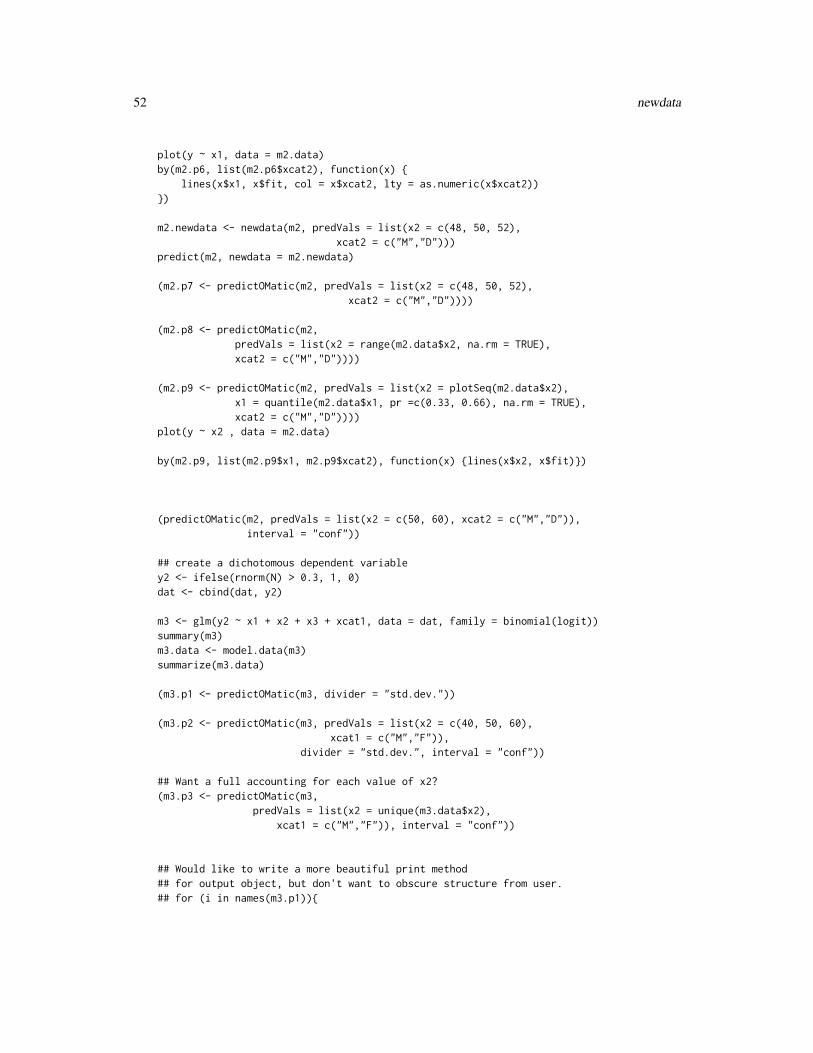
52 newdata
plot(y ~ x1, data = m2.data)by(m2.p6, list(m2.p6$xcat2), function(x) {
lines(x$x1, x$fit, col = x$xcat2, lty = as.numeric(x$xcat2))})
m2.newdata <- newdata(m2, predVals = list(x2 = c(48, 50, 52),xcat2 = c("M","D")))
predict(m2, newdata = m2.newdata)
(m2.p7 <- predictOMatic(m2, predVals = list(x2 = c(48, 50, 52),xcat2 = c("M","D"))))
(m2.p8 <- predictOMatic(m2,predVals = list(x2 = range(m2.data$x2, na.rm = TRUE),xcat2 = c("M","D"))))
(m2.p9 <- predictOMatic(m2, predVals = list(x2 = plotSeq(m2.data$x2),x1 = quantile(m2.data$x1, pr =c(0.33, 0.66), na.rm = TRUE),xcat2 = c("M","D"))))
plot(y ~ x2 , data = m2.data)
by(m2.p9, list(m2.p9$x1, m2.p9$xcat2), function(x) {lines(x$x2, x$fit)})
(predictOMatic(m2, predVals = list(x2 = c(50, 60), xcat2 = c("M","D")),interval = "conf"))
## create a dichotomous dependent variabley2 <- ifelse(rnorm(N) > 0.3, 1, 0)dat <- cbind(dat, y2)
m3 <- glm(y2 ~ x1 + x2 + x3 + xcat1, data = dat, family = binomial(logit))summary(m3)m3.data <- model.data(m3)summarize(m3.data)
(m3.p1 <- predictOMatic(m3, divider = "std.dev."))
(m3.p2 <- predictOMatic(m3, predVals = list(x2 = c(40, 50, 60),xcat1 = c("M","F")),
divider = "std.dev.", interval = "conf"))
## Want a full accounting for each value of x2?(m3.p3 <- predictOMatic(m3,
predVals = list(x2 = unique(m3.data$x2),xcat1 = c("M","F")), interval = "conf"))
## Would like to write a more beautiful print method## for output object, but don't want to obscure structure from user.## for (i in names(m3.p1)){
outreg 53
## dns <- cbind(m3.p1[[i]][i], m3.p1[[i]]$fit)## colnames(dns) <- c(i, "predicted")## print(dns)## }
outreg Creates a publication quality result table for regression models. Workswith models fitted with lm, glm, as well as lme4.
Description
This provides "markup" that the user is will copy into a LaTeX document. As of rockchalk 1.8.4,can also create HTML markup. The rockchalk vignette demonstrates use of outreg in Sweave.
Usage
outreg(modelList, type = "latex", modelLabels = NULL, varLabels = NULL,tight = TRUE, showAIC = FALSE, float = FALSE, request, runFuns,digits = 3, alpha = c(0.05, 0.01, 0.001), SElist = NULL,PVlist = NULL, Blist = NULL, title, label, gofNames,print.results = TRUE, browse = identical(type, "html") && interactive())
Arguments
modelList A regression model or an R list of regression models. Default model nameswill be M1, M2, and so forth. User specified names are allowed, such aslist("My Model" = m1,"Her Model" = m2). This is the currently rec-ommended way to supply model lables. This is less error prone than the use ofthe modelLabels argument.
type Default = "latex". The alternatives are "html" and "csv"
modelLabels This is allowed, but discouraged. A vector of character string variables, one foreach element in modelList. Will override the names in modelList.
varLabels To beautify the parameter names printed. Must be a named vector in the formatc(parmname = "displayName", parmname = "displayName"). Include as manyparameters as desired, it is not necessary to supply new labels for all of theparameters.
tight Table format. If TRUE, parameter estimates and standard errors are printed ina single column. If FALSE, parameter estimates and standard errors are printedside by side.
showAIC This is a legacy argument, before the request argument was created. If TRUE,the AIC estimate is included with the diagnostic values. It has the same effectas described by request.
float Default = FALSE. Include boilerplate for a LaTeX table float, with the tabularmarkup inside it. Not relevant if type = "html".
54 outreg
request Extra information to be retrieved from the summary(model) and displayed. Thismust be a vector of named arguments, such as c(adj.r.squared = "adj $R^2$",fstatistic = "F"). The name must be a valid name of the output object, the valueshould be the label the user wants printed in the table. See details.
runFuns A list of functions
digits Default = 3. How many digits after decimal sign are to be displayed.
alpha Default = c(0.05, 0.01, 0.001). I think stars are dumb, but enough people haveasked me for more stars that I’m caving in.
SElist Optional. Replacement standard errors. Must be a list of named vectors. outreguses the R summary to retrieve standard errors, but one might instead want touse robust or bootstrapped standard errors. This argument may supply a new SEvector for each fitted regression model, but it is also allowed to supply the SE re-placement for just one of the models. The format should be list("A Model Label" = c(0.1, 0.3, 0.4),"Another Model Label" = c(0.4, 0.2, 0.3).On the left, one must use the same names that are used in the modelList argu-ment.
PVlist Optional. A list of replacement "p values". It must be a list of named vectors,similar in format to SElist. The which the elements are the "p values" that theuser wants to use for each model.
Blist Optional. This is only needed in the rare case where a model’s parameters cannotbe discerned from its summary. List must have names for models, and vectorsslope coefficient. See discussion of SElist and PVlist.
title A LaTeX caption for the table. Not relevant if type = "html".
label A string to be used as a LaTeX label in the table to be created. Not relevant iftype = "html".
gofNames Optional pretty names. R regression summaries use names like "sigma" or"r.squared" that we might want to revise for presentation. I prefer to refer to"sigma" as "RMSE", but perhaps you instead prefer something like gofnames = c("sigma" = "ThatEstimate I don't understand", "deviance" = "Another Mystery").The words that you might replace are "sigma", "r.squared", "deviance", "adj.r.squared","fstatistic".
print.results Default TRUE, marked-up table will be displayed in session. If FALSE, sameresult is returned as an object.
browse Display the regression model in a browse? Defaults to TRUE if type = "html"
Details
outreg returns a string vector. It is suggested that users should save the outreg result and then usecat to save it. That is myMod <- outreg(m1, ...) cat(myMod, file = "myMod.html") or cat(myMod,file = "myMod.tex". In version 1.8.66, we write the html file to a temporary location and display itin a web browser. Many word processors will not accept a cut-and paste transfer from the browser,they will, however, be able to open the html file itself and automatically re-format it in the nativetable format.
In version 1.8.111, an argument print.results was introduced. This is TRUE by default, so themarked-up table is printed into the session, and it is returned as well. If the function should runsilently (as suggested in the last few versions), include print.results = TRUE.
outreg 55
The table includes a minimally sufficient (in my opinion) model summary. It offers parameterestimates, standard errors, and minimally sufficient goodness of fit. My tastes tend toward mini-mal tables, but users request more features, and outreg’s interface hass been generalized to allowspecialized requests. See request and runFuns arguments.
I don’t want to write a separate table function for every different kind of regression model that exists(how exhausting). So I’ve tried to revise outreg() to work with regression functions that followthe standard R framework. It is known to work lm and glm, as well as merMod class from lme4,but it will try to interact with other kinds of regression models. Those models should have methodssummary(), coef(), vcov() and nobs(). Package writes should provide those, its not my job.
Do you want "robust standard errors"? P values calculated according to some alternative logic?Go ahead, calculate them in your code, outreg will now accept them as arguments. As of Version1.8.4, users can provide their own standard errors and/or p-values for each model. Thus, if a modelanswers in the usual way to the standard R request coef(summary(model)), outreg can work ifusers supply standard errors.
About the customizations request. The request argument supplies a list of names of summaryoutput elements that are desired. The format is a pair, a value to be retrieved from summary(model),and a pretty name to be printed for it. With the lm() regression, for example, one might want the out-put of the F test and the adjusted R-square: Include request = c(adj.r.squared = "adj. $R^2$", "fstatistic" ="F"). The value on the left is the name of the desired information in the summary object, while thevalue on the right is any valid LaTeX (or HTML) markup that the user desires to display in the table.request terms that generate a single numerical value will generally work fine, while requests thatask for more structured information, such as the F test (including the 2 degrees of freedom values)may work (user feedback needed).
The runFuns argument is inspired by a user request: could this include the BIC or other summariesthat can be easily calculated? Any R function, such as AIC or BIC, should work, as long as it returnsa single value. This is a two-part specification, a function name and a pretty label to be used in print-ing. For example, runFuns = c("AIC" = "Akaike Criterion", "BIC" = "Schwartz Criterion", "logLik" = "LL").
Value
A character vector, one element per row of the regression table.
Note
There are many R packages that can be used to create LaTeX regression tables. memisc, texreg,apsrtable, xtables, and rms are some. This "outreg" version was in use in our labs before we wereaware that those packages were in development. It is not intended as a competitor, it is just a slightlydifferent version of the same that is more suited to our needs.
Author(s)
Paul E. Johnson <<[email protected]>>
Examples
set.seed(2134234)dat <- data.frame(x1 = rnorm(100), x2 = rnorm(100))dat$y1 <- 30 + 5 * rnorm(100) + 3 * dat$x1 + 4 * dat$x2
56 outreg
dat$y2 <- rnorm(100) + 5 * dat$x2m1 <- lm(y1 ~ x1, data = dat)m2 <- lm(y1 ~ x2, data = dat)m3 <- lm(y1 ~ x1 + x2, data = dat)gm1 <- glm(y1 ~ x1, family = Gamma, data = dat)outreg(m1, title = "My One Tightly Printed Regression", float = TRUE)ex1 <- outreg(m1, title = "My One Tightly Printed Regression",
float = TRUE, print.results = FALSE)## Show markup, Save to file with cat()cat(ex1)## cat(ex1, file = "ex1.tex")
ex2 <- outreg(list("Fingers" = m1), tight = FALSE,title = "My Only Spread Out Regressions", float = TRUE,alpha = c(0.05, 0.01, 0.001))
ex3 <- outreg(list("Model A" = m1, "Model B label with Spaces" = m2),varLabels = list(x1 = "Billie"),title = "My Two Linear Regressions", request = c(fstatistic = "F"),print.results = FALSE)
cat(ex3)
ex4 <- outreg(list("Model A" = m1, "Model B" = m2),modelLabels = c("Overrides ModelA", "Overrides ModelB"),varLabels = list(x1 = "Billie"),title = "Note modelLabels Overrides model names")
cat(ex4)
ex5 <- outreg(list("Whichever" = m1, "Whatever" = m2),title = "Still have showAIC argument, as in previous versions",showAIC = TRUE, float = TRUE)
cat(ex5)
## Launches HTML browseex5html <- outreg(list("Whichever" = m1, "Whatever" = m2),
title = "Still have showAIC argument, as in previous versions",showAIC = TRUE, type = "html")
## Could instead, make a file:## fn <- "some_name_you_choose.html"## cat(ex5html, file = fn)## browseURL(fn)## Open that HTML file in LibreOffice or MS Word
ex6 <- outreg(list("Whatever" = m1, "Whatever" =m2),title = "Another way to get AIC output",runFuns = c("AIC" = "Akaike IC"))
cat(ex6)
ex7 <- outreg(list("Amod" = m1, "Bmod" = m2, "Gmod" = m3),title = "My Three Linear Regressions", float = FALSE)
cat(ex7)
outreg 57
## A new feature in 1.85 is ability to provide vectors of beta estimates## standard errors, and p values if desired.## Suppose you have robust standard errors!newSE <- sqrt(diag(car::hccm(m3)))## See 2 versions of m3 in the table?ex8 <- outreg(list("Model A" = m1, "Model B" = m2, "Model C" = m3, "Model C w Robust SE" = m3),
SElist= list("Model C w Robust SE" = newSE))cat(ex8)
## outreg uses a t or normal approximation to calculate p values, but you can## calculate your own. Let's dial down those std errors but insist they are## not significantly different from zeronewSE <- 0.3*newSEnewPvals <- rep(0.1, length(newSE))## Pass in your own SE and P values.ex9 <- outreg(list("Model A" = m1, "Model B" = m2, "Model C" = m3),
SElist = list("Model C" = newSE),PVlist = list("Model C" = newPvals), alpha = c(0.05, 0.01, 0.001))
cat(ex9)## It took me a while to realize we might as well allow the user to## pass in a vector of Beta estimates as well. Seems obvious now, though.if(interactive()) ex10 <- outreg(list("Model C" = m3,
"Model C Robust SE" = m3, "Model C MLv2" = m3),Blist = list("Model C MLv2" = c("(Intercept)" = 0.222, "x1" = 0.222, "x2" = 0.222)),SElist = list("Model C Robust SE" = newSE, "Model C MLv2" = 1.4*newSE),PVlist = list("Model C" = newPvals),alpha = c(0.05, 0.01, 0.001), type = "html")
ex11 <- outreg(list("I Love Long Titles" = m1,"Prefer Brevity" = m2,"Short" = m3), tight = FALSE, float = FALSE)
cat(ex11)
ex12 <- outreg(list("GLM" = gm1), float = TRUE)cat(ex12)
ex13 <- outreg(list("OLS" = m1, "GLM" = gm1), float = TRUE,alpha = c(0.05, 0.01))
cat(ex13)
ex14 <- outreg(list(OLS = m1, GLM = gm1), float = TRUE,request = c(fstatistic = "F"), runFuns = c("BIC" = "BIC"))
cat(ex14)
ex15 <- outreg(list(OLS = m1, GLM = gm1), float = TRUE,request = c(fstatistic = "F"), runFuns = c("BIC" = "BIC"),digits = 5, alpha = c(0.01))
ex16 <- outreg(list("OLS 1" = m1, "OLS 2" = m2, GLM = gm1), float = TRUE,request = c(fstatistic = "F"),runFuns = c("BIC" = "BIC", logLik = "ll"),
58 outreg0
digits = 5, alpha = c(0.05, 0.01, 0.001))
ex17 <- outreg(list("Model A" = gm1, "Model B label with Spaces" = m2),request = c(fstatistic = "F"),runFuns = c("BIC" = "Schwarz IC", "AIC" = "Akaike IC","nobs" = "N Again?"))
## Here's a fit example from lme4.if (require(lme4)){
fm1 <- lmer(Reaction ~ Days + (Days | Subject), sleepstudy)ex18 <- outreg(fm1)cat(ex18)## Fit same with lm for comparisonlm1 <- lm(Reaction ~ Days, sleepstudy)## Get robust standard errorslm1rse <- sqrt(diag(car::hccm(lm1)))
if(interactive()){ex19 <- outreg(list("Random Effects" = fm1,
"OLS" = lm1, "OLS Robust SE" = lm1),SElist = list("OLS Robust SE" = lm1rse), type = "html")
}## From the glmer examplesgm2 <- glmer(cbind(incidence, size - incidence) ~ period + (1 | herd),
data = cbpp, family = binomial)lm2 <- lm(incidence/size ~ period, data = cbpp)lm2rse <- sqrt(diag(car::hccm(lm2)))## Lets see what MASS::rlm objects do? Mostly OKrlm2 <- MASS::rlm(incidence/size ~ period, data = cbpp)
ex20 <- outreg(list("GLMER" = gm2, "lm" = lm2, "lm w/robust se" = lm2,"rlm" = rlm2), SElist = list("lm w/robust se" = lm2rse),type = "html")
}
outreg0 Creates a publication quality result table for regression models. out-reg0 is the last version in the last development stream.
Description
outreg0 writes its output directly to the terminal, but does not create an output object. The newversion of this function–which I wish you would try instead–does the same work, but it also createsan output object that can be transformed for other purposes.
Usage
outreg0(modelList, title, label, modelLabels = NULL, varLabels = NULL,tight = TRUE, showAIC = FALSE, float = FALSE, request, runFuns,digits = 3, alpha = 0.05)
outreg0 59
Arguments
modelList A regression model or an R list of regression models. If this is a named list,the names will be used as column labels, unless the argument modelLabels issupplied separately, which will override the names of modelList.
title A title to be displayed on the top of the LaTeX regression table.
label A string to be used as a LaTeX label in the table to be created.
modelLabels A vector of charater string variables, one for each element in modelList. Willoverride the names in modelList.
varLabels To beautify the parameter names printed. Must be a named vector in the formatc(parmname = "displayName", parmname = "displayName"). Include as manyparameters as desired, it is not necessary to supply new labels for all of theparameters. "displayName" must be valid laTeX. This feature is useful if yourvariable names have any illegal LaTeX characters, such as "$" or "_".
tight If TRUE, parameter estimates and standard errors are printed in a single column.If FALSE, parameter estimates and standard errors are printed side by side.
showAIC If TRUE, the AIC estimate is included with the diagnostic values
float Include boilerplate for a table float, with the tabular markup inside it.
request Extra information to be retrieved from the summary(model) and displayed. Thismust be a vector of named arguments, such as c(adj.r.squared = "adj $R^2$",fstatistic = "F"). The name must be a valid name of the output object, the valueshould be the label the user wants printed in the table. See details.
runFuns A list of functions
digits Default = 3. How many digits after decimal sign are to be displayed.
alpha Default = 0.05. I think stars are dumb, but enough people have asked me formore stars that I’m caving in. Enter c(0.05, 0.01, 0.001) to see what happens.
Details
This provides "markup" that the user is will copy into a LaTeX document. The table is a LaTeXtabular environment, which can be enclosed in a table to obtain a "floating," automatically numberedLaTeX document environment. The default will create the tabular-inside-a-table, but if only thetabular is needed, use the argument float = FALSE. This can be called within Sweave documents.The markup generated by the basic usage will generally be presentable as is, while user requests foradditional details may cause output that needs some hand-editing.
A LaTeX tabular object is created, with the floating table markup around it if requested (float =TRUE).
The table include a minimally sufficient (in my opinion) model summary. For any fitted model,outreg0() will present the parameter estimates and standard errors, and it will also scan the sum-mary of the object for some summary values and goodness of fit indicators. Some users may wantmore information. lm fits will not include output for the "fstatistic" that is reported in the lm’s sum-mary object, but users can ask for it with the argument request. Similarly, the argument runFunscan ask for additional diagnostic functions to be reported.
While outreg0() originally designed for models fitted by lm() and glm(), it will now work forany kind of regression model that has methods summary(), coef(), vcov() and nobs(). This will
60 outreg0
not succeed, however, if the regression model’s summary function does not create an object thatholds values in a workable structure (in the same way that lm() and glm() do). Please pressurepeople who write R packages that claim to "do regression" to supply methods to do the basic workthat we need to compile tables.
Two types of customization arguments were introduced with rockchalk version 1.7.3. The newarguments are request and runFuns. Beta test reports are welcome!
The request argument supplies a list of names of summary output elements that are desired. Theformat is a pair, a value to be retrieved and a name to be printed for it. With the lm() regression, forexample, one might want the output of the F test and the adjusted R-square. An example usage mightbe request = c(adj.r.squared = "adj. $R^2", fstatistic = "F"). The names may be in-cluded in quotation marks if the user desires to do so: request = c("adj.r.squared" = "adj. $R^2","fstatistic" = "F").The value on the left is the name of the desired information in the summary object, while the valueon the right is any valid LaTeX markup that the user desires to display in the first column of thetable. request terms that generate a single numerical value will generally work fine, while requeststhat ask for more structured information, such as the F test (including the 2 degrees of freedomvalues) are still a work in progress.
The runFuns argument is inspired by a user request: could this include the BIC or other summariesthat some models report? We have to run the BIC function, and divert the result into the correctcolumn of the result table. Any R function, whether supplied with and R package or in the user’sown code, may be used. This is a two-part specification, one representing the function to be run,the other representing the name that is desired in the output. For example, it might be runFuns =c("AIC" = "Akaike Criterion", "BIC" = "Schwartz Criterion","logLik" = "LL").
Value
None
Note
There are many R packages that can be used to create LaTeX regression tables. memisc, texreg,apsrtable, xtables, and rms are some. This "outreg" version was in use in our labs before we wereaware that those packages were in development. It is not intended as a competitor, it is just a slightlydifferent version of the same that is more suited to our needs.
Author(s)
Paul E. Johnson <<[email protected]>>
Examples
set.seed(2134234)dat <- data.frame(x1 = rnorm(100), x2 = rnorm(100))dat$y1 <- 30 + 5 * rnorm(100) + 3 * dat$x1 + 4 * dat$x2dat$y2 <- rnorm(100) + 5 * dat$x2m1 <- lm(y1 ~ x1, data = dat)m2 <- lm(y1 ~ x2, data = dat)m3 <- lm(y1 ~ x1 + x2, data = dat)gm1 <- glm(y1 ~ x1, family = Gamma, data = dat)
outreg0 61
outreg0(list("Model 1" = m1), title = "My One Tightly Printed Regression")
outreg0(list("Model 1" = m1), title = "My One Tightly Printed Regression in aFloat", float = TRUE, label = "outreg1")
outreg0(list("Fingers" = m1), tight = FALSE, title = "My OnlySpread Out Regression", float = TRUE, alpha = c(0.05, 0.01,0.001))
outreg0(list(ModelA = m1, "Model B label with Spaces" = m2),varLabels = list(x1 = "Billie"),title = "My Two Linear Regressions",request = c(fstatistic = "F"))
outreg0(list(ModelA = m1, ModelB = m2),modelLabels = c("Overrides ModelA", "Overrides ModelB"),varLabels = list(x1 = "Billie"),title = "Note modelLabels Overrides model names")
outreg0(list(m1, m2), modelLabels = c("Whatever", "Whichever"),title = "Still have showAIC argument, as in previous versions",showAIC = TRUE, float = TRUE)
outreg0(list(m1, m2), modelLabels = c("Whatever", "Whichever"),title = "Another way to get AIC output",runFuns = c("AIC" = "Akaike IC"))
outreg0(list("Amod" = m1, "Bmod" = m2, "Gmod" = m3),title = "My Three Linear Regressions", float = FALSE)
outreg0(list(m1, m2, m3), tight = FALSE,modelLabels = c("I Love really long titles", "Hate Long", "Medium"),float = FALSE)
outreg0(list(gm1), modelLabels = c("GLM"), float = TRUE)
outreg0(list(m1, gm1), modelLabels = c("OLS", "GLM"),float = TRUE, alpha = c(0.05, 0.01))
outreg0(list(OLS = m1, GLM = gm1), float = TRUE,request = c(fstatistic = "F"), runFuns = c("BIC" = "BIC"))
outreg0(list(OLS = m1, GLM = gm1), float = TRUE,request = c(fstatistic = "F"), runFuns = c("BIC" = "BIC"),digits = 5, alpha = 0.01)
outreg0(list("OLS 1" = m1, "OLS 2" = m2, GLM = gm1), float = TRUE,request = c(fstatistic = "F"),runFuns = c("BIC" = "BIC", logLik = "ll"),digits = 5, alpha = c(0.05, 0.01, 0.001))
outreg0(list(ModelA = gm1, "Model B label with Spaces" = m2),request = c(fstatistic = "F"),
62 outreg2HTML
runFuns = c("BIC" = "Schwarz IC", "AIC" = "Akaike IC","nobs" = "N Again?"))
outreg2HTML Convert LaTeX output from outreg to HTML markup
Description
This function is deprecated. Instead, please use outreg(type = "html")
Usage
outreg2HTML(outreg, filename)
Arguments
outreg output from outreg
filename A file name into which the regression markup is to be saved. Should end in.html.
Details
This will write the html on the screen, but if a filename argument is supplied, it will write a file.One can then open or insert the file into Libre Office or other popular "word processor" programs.
Value
A vector of strings
Author(s)
Paul E. Johnson <<[email protected]>>
Examples
dat <- genCorrelatedData2(means = c(50,50,50,50,50,50),sds = c(10,10,10,10,10,10), rho = 0.2, beta = rnorm(7), stde = 50)
m1 <- lm(y ~ x1 + x2 + x3 + x4 + x5 + x6 + x1*x2, data = dat)summary(m1)
m1out <- outreg(list("Great Regression" = m1), alpha = c(0.05, 0.01, 0.001),request = c("fstatistic" = "F"), runFuns = c(AIC = "AIC"),float = TRUE)
##html markup will appear on screenoutreg2HTML(m1out)## outreg2HTML(m1out, filename = "funky.html")## I'm not running that for you because you## need to be in the intended working directory
padW0 63
m2 <- lm(y ~ x1 + x2, data = dat)
m2out <- outreg(list("Great Regression" = m1, "Small Regression" = m2),alpha = c(0.05, 0.01, 0.01),request = c("fstatistic" = "F"), runFuns = c(BIC = "BIC"))
outreg2HTML(m2out)## Run this for yourself, it will create the output file funky2.html## outreg2HTML(m2out, filename = "funky2.html")## Please inspect the file "funky2.html
padW0 Pad with 0’s.
Description
Sometimes we receive this c(1, 22, 131) and we need character variables of the same size, such asc("001", "022", "131"). This happens if a user has mistakenly converted a zip code (US regionalidentifier) like "00231" to a number. This function converts the number back to a 0 padded string.
Usage
padW0(x)
Arguments
x a numeric variable.
Details
This works differently if the number provided is an integer, or a character string. Integers are leftpadded with the character "0". A character string will be left-padded with blanks.
Value
A character string vector padded with 0’s
Author(s)
Paul Johnson <[email protected]>
Examples
x <- c(1 , 11, 22, 121, 14141, 31)(xpad <- padW0(x))x <- rpois(7, lambda = 11)(xpad <- padW0(x))x <- c("Alabama", "Iowa", "Washington")
64 pctable
pctable Creates a cross tabulation with counts and percentages
Description
This function is pronounced "presentable"! The original purpose was to create a particular kindof cross tabulation that I ask for in class: counts with column percentages. Requests from usershave caused a bit more generality to be built into the function. Now, optionally, it will provide rowpercents. This is a generic function. Most users will find the formula method most convenient. Usethe colpct and rowpct arguments to indicate if column or row percentages are desired.
I suggest most users will use the formula method for this. Running a command like this will,generally, do the right thing:
tab <- pctable(y ~ x, data = dat)
There is also a method that will work with characters representing variable names.
tab <- pctable("y", "x", data = dat)
Running the function should write a table in the output console, but it also creates an object (tab).That object can be displayed in a number of ways.
A summary method is provided, so one could look at different representations of the same table.
summary(tab, rowpct = TRUE, colpct = FALSE)
or
summary(tab, rowpct = TRUE, colpct = TRUE)
Tables that include only row or column percentages will be compatible with the html and latexexporters in the excellent tables package.
The method pctable.default is the calculator, I don’t expect many users will need to call it directly.
The formula method is the recommended method for users. Run pctable(myrow ~ mycol, data = dat).In an earlier version, I gave different advice, so please adjust your usage.
The character method exists only for variety. It accepts character strings rather than a formula todefine the columns that should be plotted. The method used most often for most users should be theformula method.
Usage
pctable(rv, ...)
## Default S3 method:pctable(rv, cv, rvlab = NULL, cvlab = NULL,colpct = TRUE, rowpct = FALSE, rounded = FALSE, ...)
## S3 method for class 'formula'pctable(formula, data = NULL, rvlab = NULL,cvlab = NULL, colpct = TRUE, rowpct = FALSE, rounded = FALSE, ...)
pctable 65
## S3 method for class 'character'pctable(rv, cv, data = NULL, rvlab = NULL,cvlab = NULL, colpct = TRUE, rowpct = FALSE, rounded = FALSE, ...)
Arguments
rv A row variable name
... Other arguments. So far, the most likely additional arguments are to be passedalong to the table function, such as "exclude", "useNA", or "dnn" (which willoverride the rvlab and cvlab arguments provided by some methods). Somemethods will also pass along these arguments to model.frame, "subset" "xlev","na.action", "drop.unused.levels".
cv Column variable
rvlab Optional: row variable label
cvlab Optional: col variable label
colpct Default TRUE: are column percentags desired in the presentation of this result?
rowpct Default FALSE: are row percentages desired in the presentation of this result
rounded Default FALSE, rounds to 10’s for privacy purposes.
formula A two sided formula.
data A data frame.
Details
Please bear in mind the following. The output object is a list of tables of partial information, whichare then assembled in various ways by the print method (print.pctable). A lovely table will appearon the screen, but the thing itself has more information and a less beautiful structure.
A print method is supplied. For any pctable object, it is possible to run follow-ups like
print(tab, rowpct = TRUE, colpct = FALSE)
The method print.pctable(tab) assembles the object into (my opinion of) a presentable form.The print method has argumnets rowpct and colpct that determine which percentages are includedin the presentation.
When using character arguments, the row variable rv rowvar must be a quoted string if the userintends the method pctable.character to be dispatched. The column variable cv may be a string orjust a variable name (which this method will coerce to a string).
Value
A list with tables (count, column percent, row percent) as well as a copy of the call.
Author(s)
Paul Johnson <[email protected]>
See Also
tabular and the CrossTable function in gmodels package.
66 perspEmpty
Examples
dat <- data.frame(x = gl(4, 25),y = sample(c("A", "B", "C", "D", "E"), 100, replace= TRUE))
pctable(y ~ x, dat)pctable(y ~ x, dat, exclude = NULL)pctable(y ~ x, dat, rvlab = "My Outcome Var", cvlab = "My Columns")pctable(y ~ x, dat, rowpct = TRUE, colpct = FALSE)pctable(y ~ x, dat, rowpct = TRUE, colpct = TRUE)pctable(y ~ x, dat, rowpct = TRUE, colpct = TRUE, exclude = NULL)tab <- pctable(y ~ x, dat, rvlab = "Outcome", cvlab = "Predictor")dat <- data.frame(x1 = gl(4, 25, labels = c("Good", "Bad", "Ugly", "Indiff")),
x2 = gl(5, 20, labels = c("Denver", "Cincy", "Baltimore", "NY", "LA")),y = sample(c("A", "B", "C", "D", "E"), 100, replace= TRUE))
tab <- pctable(y ~ x1, data = dat, rvlab = "my row label",subset = dat$x1 %in% c("Good", "Bad"),drop.unused.levels = TRUE)
tab <- pctable(y ~ x1, data = dat, rvlab = "my row label",subset = dat$x1 %in% c("Good", "Bad"))
pctable("y", "x1", dat)pctable("y", x1, dat)tab <- pctable(y ~ x2, data = dat, rvlab = "A Giant Variable")summary(tab, rowpct = TRUE, colpct = FALSE)tabsum <- summary(tab)
## if user has tables package, can push out to latex or htmlif (require(tables) & require(Hmisc)){
tabsumtab <- tables::as.tabular(tabsum)Hmisc::html(tabsumtab)fn <- tempfile(pattern = "file", tmpdir = tempdir(),
fileext = ".html")Hmisc::html(tabsumtab, file = fn)print(paste("The file saved was named", fn, "go get it."))if (interactive()) browseURL(fn)## go get the fn file if you want to import it in document## Now LaTeX output## have to escape the percent signstabsumtab <- apply(tabsumtab, 1:2, function(x) {gsub("%", "\\\\%", x) })fn2 <- tempfile(pattern = "file", tmpdir = tempdir(),
fileext = ".tex")Hmisc::latex(tabsumtab, file = fn2)print(paste("The file saved was named", fn2, "go get it."))
}
perspEmpty perspEmpty
Description
Creates a persp plot without drawing anything in the interior. Does equivalent of plot( type="n")for persp.
perspEmpty 67
Usage
perspEmpty(x1, x2, y, x1lab = "x1", x2lab = "x2", ylab = "y", x1lim,x2lim, ...)
Arguments
x1 data for the first horizontal axis, an R vector
x2 data for the second horizontal axis, an R vector
y data for the vertical axis, an R vector
x1lab label for the x1 axis, (the one called "xlab" inside persp)
x2lab label for the x2 axis, (the one called "ylab" inside persp)
ylab label for the y (vertical) axis (the one called "zlab" inside persp)
x1lim Optional: limits for x1 axis (should be a vector with 2 elements)
x2lim Optional: limits for x2 axis (should be a vector with 2 elements)
... further arguments that are passed to persp. Please note Please remember thaty is the vertical axis, but for persp, that is the one I call x2. Thus dot-dot-dot arguments including xlab, ylab, zlab, xlim, ylim, and zlim are going to beignored.
Details
Regression demonstrations require a blank slate in which points and planes can be drawn. Thisfunction creates that blank persp canvas for those projects. It is not necessary that x1, x2 and y bevectors of the same length, since this function’s only purpose is to plot an empty box with rangesdetermined by the input variables. persp calls the 3 axes x, y, and z, but here they are called x1, x2,and y.
Value
The perspective matrix that is returned by persp
Examples
x1 <- 1:10x2 <- 41:50y <- rnorm(10)perspEmpty(x1, x2, y)res <- perspEmpty(x1, x2, y, ticktype="detailed", nticks=10)mypoints1 <- trans3d ( x1, x2, y, pmat = res )points( mypoints1, pch = 16, col= "blue")
68 plotCurves
plot.testSlopes Plot testSlopes objects
Description
plot.testSlopes is a method for the generic function plot. It has been revised so that it creates aplot illustrating the marginal effect, using the Johnson-Neyman interval calculations to highlightthe "statistically significantly different from zero" slopes.
Usage
## S3 method for class 'testSlopes'plot(x, ..., shade = TRUE, col = rgb(1, 0, 0, 0.1))
Arguments
x A testSlopes object.
... Additional arguments that are ignored currently.
shade Optional. Create colored polygon for significant regions.
col Optional. Color of the shaded area. Default transparent pink.
Value
NULL
Author(s)
plotCurves Assists creation of predicted value curves for regression models.
Description
Creates a predicted value plot that includes a separate predicted value line for each value of afocal variable. The x axis variable is specified by the plotx argument. As of rockchalk 1.7.x, themoderator argument, modx, is optional. Think of this a new version of R’s termplot, but it allowsfor interactions. And it handles some nonlinear transformations more gracefully than termplot.
Usage
plotCurves(model, plotx, nx = 40, modx, plotxRange = NULL, n,modxVals = NULL, interval = c("none", "confidence", "prediction"),plotPoints = TRUE, plotLegend = TRUE, legendTitle = NULL,legendPct = TRUE, col = NULL, llwd = 2, opacity = 100,envir = environment(formula(model)), ...)
plotCurves 69
Arguments
model Required. Fitted regression object. Must have a predict method
plotx Required. String with name of predictor for the x axis
nx Number of values of plotx at which to calculate the predicted value. Default =40.
modx Optional. String for moderator variable name. May be either numeric or factor.
plotxRange Optional. If not specified, the observed range of plotx will be used to determinethe axis range.
n Optional. Number of focal values of modx, used by algorithms specified bymodxVals; will be ignored if modxVals supplies a vector of focal values.
modxVals Optional. A vector of focal values for which predicted values are to be plotted.May also be a character string to select an algorithm ("quantile","std.dev." or"table"), or a user-supplied function to select focal values (a new method similarto getFocal). If modx is a factor, currently, the only available algorithm is"table" (see getFocal.factor.
interval Optional. Intervals provided by the predict.lm may be supplied, either "conf"(95 interval for the estimated conditional mean) or "pred" (95 interval for ob-served values of y given the rest of the model).
plotPoints Optional. TRUE or FALSE: Should the plot include the scatterplot points alongwith the lines.
plotLegend Optional. TRUE or FALSE: Should the default legend be included?
legendTitle Optional. You’ll get an automatically generated title, such as "Moderator: modx",but if you don’t like that, specify your own string here.
legendPct Default = TRUE. Variable labels print with sample percentages.
col Optional. A color vector to differentiate the moderator values in the plot. Ifnot specified, the R’s builtin palette() will be used. User may supply a vectorof valid color names, either explicitly c("pink","black", "gray70") or implicitly,rainbow(10) or gray.colors(5). Color names will be recycled if there are morefocal values of modx than colors provided.
llwd Optional. Line widths for predicted values. Can be single value or a vector,which will be recycled as necessary.
opacity Optional, default = 100. A number between 1 and 255. 1 means "transparent"or invisible, 255 means very dark. the darkness of confidence interval regions
envir environment to search for variables.
... further arguments that are passed to plot or predict. The arguments that aremonitored to be sent to predict are c("type", "se.fit", "dispersion", "interval","level", "terms", "na.action").
Details
This is similar to plotSlopes, but it accepts regressions in which there are transformed variables,such as "log(x1)". It creates a plot of the predicted dependent variable against one of the numericpredictors, plotx. It draws a predicted value line for each value of modx, a moderator variable. Themoderator may be a numeric or categorical moderator variable.
70 plotCurves
The user may designate which particular values of the moderator are used for calculating the pre-dicted value lines. That is, modxVals = c( 12,22,37) would draw lines for values 12, 22, and37 of the moderator. User may instead supply a character string to choose one of the built in algo-rithms. The default algorithm is "quantile", which will select n values that are evenly spaced alongthe modx axis. The algorithm "std.dev" will select the mean of modx (m) and then it will selectvalues that step away from the mean in standard deviation sd units. For example, if n = 3, the focalvalues will m, m - sd, am + sd.
Value
A plot is created as a side effect, a list is returned including 1) the call, 2) a newdata object thatincludes information on the curves that were plotted, 3) a vector modxVals, the values for whichcurves were drawn.
Author(s)
Paul E. Johnson <[email protected]>
Examples
library(rockchalk)
## Replicate some R classics. The budworm.lg data from predict.glm## will work properly after re-formatting the information as a data.frame:
## example from Venables and Ripley (2002, pp. 190-2.)df <- data.frame(ldose = rep(0:5, 2),
sex = factor(rep(c("M", "F"), c(6, 6))),SF.numdead = c(1, 4, 9, 13, 18, 20, 0, 2, 6, 10, 12, 16))
df$SF.numalive = 20 - df$SF.numdead
budworm.lg <- glm(cbind(SF.numdead, SF.numalive) ~ sex*ldose, data = df,family = binomial)
plotCurves(budworm.lg, plotx = "ldose", modx = "sex", interval = "confidence",ylim = c(0, 1))
## See infertmodel2 <- glm(case ~ age + parity + education + spontaneous + induced,
data = infert, family = binomial())
## Curvature so slight we can barely see itmodel2pc1 <- plotCurves(model2, plotx = "age", modx = "education",
interval = "confidence", ylim = c(0, 1))
model2pc2 <- plotCurves(model2, plotx = "age", modx = "education",modxVals = levels(infert$education)[1],interval = "confidence", ylim = c(0, 1))
plotCurves 71
model2pc2 <- plotCurves(model2, plotx = "age", modx = "education",modxVals = levels(infert$education)[c(2,3)],interval = "confidence", ylim = c(0, 1))
model2pc2 <- plotCurves(model2, plotx = "age", modx = "education",modxVals = levels(infert$education)[c(2,3)],ylim = c(0, 1), type = "response")
## Manufacture some dataset.seed(12345)N <- 500dat <- genCorrelatedData2(N = 500, means = c(5, 0, 0, 0), sds = rep(1, 4),
rho = 0.2, beta = rep(1, 5), stde = 20)
dat$xcat1 <- gl(2, N/2, labels = c("Monster", "Human"))dat$xcat2 <- cut(rnorm(N), breaks = c(-Inf, 0, 0.4, 0.9, 1, Inf),
labels = c("R", "M", "D", "P", "G"))
###The design matrix for categorical variables, xcat numericdat$xcat1n <- with(dat, contrasts(xcat1)[xcat1, ])dat$xcat2n <- with(dat, contrasts(xcat2)[xcat2, ])
stde <- 2dat$y <- with(dat, 0.03 + 11.5 * log(x1) * contrasts(dat$xcat1)[dat$xcat1] +
0.1 * x2 + 0.04 * x2^2 + stde*rnorm(N))
stde <- 1dat$y2 <- with(dat, 0.03 + 0.1 * x1 + 0.1 * x2 + 0.25 * x1 * x2 + 0.4 * x3 -
0.1 * x4 + stde * rnorm(N))stde <- 8dat$y3 <- with(dat, 3 + 0.5 * x1 + 1.2 * (as.numeric(xcat1)-1) +-0.8 * (as.numeric(xcat1)-1) * x1 + stde * rnorm(N))
stde <- 8dat$y4 <- with(dat, 3 + 0.5 * x1 +
contrasts(dat$xcat2)[dat$xcat2, ] %*% c(0.1, -0.2, 0.3, 0.05) +stde * rnorm(N))
## Curvature with interactionm1 <- lm(y ~ log(x1)*xcat1 + x2 + I(x2^2), data=dat)summary(m1)
## First, with no moderatorplotCurves(m1, plotx = "x1")
plotCurves(m1, plotx = "x1", modx = "xcat1")
72 plotCurves
## ## Verify that plot by comparing against a manually contructed alternative## par(mfrow=c(1,2))## plotCurves(m1, plotx = "x1", modx = "xcat1")## newdat <- with(dat, expand.grid(x1 = plotSeq(x1, 30), xcat1 = levels(xcat1)))## newdat$x2 <- with(dat, mean(x2, na.rm = TRUE))## newdat$m1p <- predict(m1, newdata = newdat)## plot( y ~ x1, data = dat, type = "n", ylim = magRange(dat$y, c(1, 1.2)))## points( y ~ x1, data = dat, col = dat$xcat1, cex = 0.4, lwd = 0.5)## by(newdat, newdat$xcat1, function(dd) {lines(dd$x1, dd$m1p)})## legend("topleft", legend=levels(dat$xcat1), col = as.numeric(dat$xcat1), lty = 1)## par(mfrow = c(1,1))## ##Close enough!
plotCurves(m1, plotx = "x2", modx = "x1")
plotCurves(m1, plotx = "x2", modx = "xcat1")
plotCurves(m1, plotx = "x2", modx = "xcat1", interval = "conf")
m2 <- lm(y ~ log(x1)*xcat1 + xcat1*(x2 + I(x2^2)), data = dat)summary(m2)plotCurves(m2, plotx = "x2", modx = "xcat1")
plotCurves(m2, plotx ="x2", modx = "x1")
m3a <- lm(y ~ poly(x2, 2) + xcat1, data = dat)
plotCurves(m3a, plotx = "x2")plotCurves(m3a, plotx = "x2", modx = "xcat1")#OK
m4 <- lm(log(y+10) ~ poly(x2, 2)*xcat1 + x1, data = dat)summary(m4)plotCurves(m4, plotx = "x2")
plotCurves(m4, plotx ="x2", modx = "xcat1")
plotCurves(m4, plotx = "x2", modx = "x1")
plotCurves(m4, plotx = "x2", modx = "xcat1")
plotCurves(m4, plotx = "x2", modx = "xcat1", modxVals = c("Monster"))
##ordinary interactionm5 <- lm(y2 ~ x1*x2 + x3 +x4, data = dat)summary(m5)plotCurves(m5, plotx = "x1", modx = "x2")plotCurves(m5, plotx = "x1", modx = "x2", modxVals = c( -2, -1, 0, 1, 2))
plotFancy 73
plotCurves(m5, plotx = "x1", modx = "x2", modxVals = c(-2))plotCurves(m5, plotx = "x1", modx = "x2", modxVals = "std.dev.")plotCurves(m5, plotx = "x1", modx = "x2", modxVals = "quantile")plotCurves(m5, plotx = "x3", modx = "x2")
library(car)mc1 <- lm(statusquo ~ income * sex, data = Chile)summary(mc1)plotCurves(mc1, plotx = "income")plotCurves(mc1, modx = "sex", plotx = "income")plotCurves(mc1, modx = "sex", plotx = "income", modxVals = "M")
mc2 <- lm(statusquo ~ region * income, data = Chile)summary(mc2)plotCurves(mc2, modx = "region", plotx = "income")plotCurves(mc2, modx = "region", plotx = "income",
modxVals = levels(Chile$region)[c(1,4)])plotCurves(mc2, modx = "region", plotx = "income", modxVals = c("S","M","SA"))plotCurves(mc2, modx = "region", plotx = "income", modxVals = c("S","M","SA"),
interval = "conf")
plotCurves(mc2, modx = "region", plotx = "income", plotPoints = FALSE)
mc3 <- lm(statusquo ~ region * income + sex + age, data = Chile)summary(mc3)plotCurves(mc3, modx = "region", plotx = "income")
mc4 <- lm(statusquo ~ income * (age + I(age^2)) + education + sex + age, data = Chile)summary(mc4)plotCurves(mc4, plotx = "age")plotCurves(mc4, plotx = "age", interval = "conf")
plotCurves(mc4, plotx = "age", modx = "income")plotCurves(mc4, plotx = "age", modx = "income", plotPoints = FALSE)
plotCurves(mc4, plotx = "income", modx = "age")plotCurves(mc4, plotx = "income", modx = "age", n = 8)
plotCurves(mc4, plotx = "income", modx = "age", modxVals = "std.dev.")plotCurves(mc4, modx = "income", plotx = "age", plotPoints = FALSE)
plotFancy Regression plots with predicted value lines, confidence intervals, colorcoded interactions
74 plotPlane
Description
This is the back-end for the functions plotSlopes and plotCurves. Don’t use it directly.
Usage
plotFancy(newdf, olddf, plotx, modx, modxVals, interval, plotPoints, plotLegend,legendTitle, col = NULL, llwd = 2, opacity, ...)
Arguments
newdf The new data frame with predictors and fit, lwr, upr variables
olddf A data frame with variables(modxVar, plotxVar, depVar)
plotx Character string for name of variable on horizontal axis
modx Character string for name of moderator variable.
modxVals Values of moderator for which lines are desired
interval TRUE or FALSE: want confidence intervals?
plotPoints TRUE or FALSE: want to see observed values in plot?
plotLegend TRUE or FALSE: draw defaut legend
legendTitle Optional. You’ll get an automatically generated title, such as "Moderator: modx",but if you don’t like that, specify your own string here.
col requested color scheme for lines and points. One per value of modxVals.
llwd requested line width, will re-cycle.
opacity Value in 0, 255 for darkness of interval shading
... Other arguments passed to plot function.
Value
col, lty, and lwd information
Author(s)
Paul E. Johnson <[email protected]>
plotPlane Draw a 3-D regression plot for two predictors from any linear or non-linear lm or glm object
plotPlane 75
Description
This allows user to fit a regression model with many variables and then plot 2 of its predictorsand the output plane for those predictors with other variables set at mean or mode (numeric orfactor). This is a front-end (wrapper) for R’s persp function. Persp does all of the hard work, thisfunction reorganizes the information for the user in a more readily understood way. It intended as aconvenience for students (or others) who do not want to fight their way through the details neededto use persp to plot a regression plane. The fitted model can have any number of input variables,this will display only two of them. And, at least for the moment, I insist these predictors must benumeric variables. They can be transformed in any of the usual ways, such as poly, log, and soforth.
Usage
plotPlane(model = NULL, plotx1 = NULL, plotx2 = NULL,drawArrows = FALSE, plotPoints = TRUE, npp = 20, x1lab, x2lab, ylab,x1lim, x2lim, x1floor = 5, x2floor = 5, pch = 1, pcol = "blue",plwd = 0.5, pcex = 1, llwd = 0.3, lcol = 1, llty = 1,acol = "red", alty = 4, alwd = 0.3, alength = 0.1, linesFrom,lflwd = 3, envir = environment(formula(model)), ...)
## Default S3 method:plotPlane(model = NULL, plotx1 = NULL, plotx2 = NULL,drawArrows = FALSE, plotPoints = TRUE, npp = 20, x1lab, x2lab, ylab,x1lim, x2lim, x1floor = 5, x2floor = 5, pch = 1, pcol = "blue",plwd = 0.5, pcex = 1, llwd = 0.3, lcol = 1, llty = 1,acol = "red", alty = 4, alwd = 0.3, alength = 0.1, linesFrom,lflwd = 3, envir = environment(formula(model)), ...)
Arguments
model an lm or glm fitted model object
plotx1 name of one variable to be used on the x1 axis
plotx2 name of one variable to be used on the x2 axis
drawArrows draw red arrows from prediction plane toward observed values TRUE or FALSE
plotPoints Should the plot include scatter of observed scores?
npp number of points at which to calculate prediction
x1lab optional label
x2lab optional label
ylab optional label
x1lim optional lower and upper bounds for x1, as vector like c(0,1)
x2lim optional lower and upper bounds for x2, as vector like c(0,1)
x1floor Default=5. Number of "floor" lines to be drawn for variable x1
x2floor Default=5. Number of "floor" lines to be drawn for variable x2
pch plot character, passed on to the "points" function
76 plotPlane
pcol color for points, col passed to "points" function
plwd line width, lwd passed to "points" function
pcex character expansion, cex passed to "points" function
llwd line width, lwd passed to the "lines" function
lcol line color, col passed to the "lines" function
llty line type, lty passed to the "lines" function
acol color for arrows, col passed to "arrows" function
alty arrow line type, lty passed to the "arrows" function
alwd arrow line width, lwd passed to the "arrows" function
alength arrow head length, length passed to "arrows" function
linesFrom object with information about "highlight" lines to be added to the 3d plane (out-put from plotCurves or plotSlopes)
lflwd line widths for linesFrom highlight lines
envir environment from whence to grab data
... additional parameters that will go to persp
Details
Besides a fitted model object, plotPlane requires two additional arguments, plotx1 and plotx2. Theseare the names of the plotting variables. Please note, that if the term in the regression is somethinglike poly(fish,2) or log(fish), then the argument to plotx1 should be the quoted name of the variable"fish". plotPlane will handle the work of re-organizing the information so that R’s predict functionscan generate the desired information. This might be thought of as a 3D version of "termplot", witha significant exception. The calculation of predicted values depends on predictors besides plotx1and plotx2 in a different ways. The sample averages are used for numeric variables, but for factorsthe modal value is used.
This function creates an empty 3D drawing and then fills in the pieces. It uses the R functionslines, points, and arrows. To allow customization, several parameters are introduced for theusers to choose colors and such. These options are prefixed by "l" for the lines that draw the plane,"p" for the points, and "a" for the arrows. Of course, if plotPoints=FALSE or drawArrows=FALSE,then these options are irrelevant.
Value
The main point is the plot that is drawn, but for record keeping the return object is a list including1) res: the transformation matrix that was created by persp 2) the call that was issued, 3) x1seq, the"plot sequence" for the x1 dimension, 4) x2seq, the "plot sequence" for the x2 dimension, 5) zplane,the values of the plane corresponding to locations x1seq and x2seq.
Author(s)
Paul E. Johnson <[email protected]>
See Also
persp, scatterplot3d, regr2.plot
plotPlane 77
Examples
library(rockchalk)
set.seed(12345)x1 <- rnorm(100)x2 <- rnorm(100)x3 <- rnorm(100)x4 <- rnorm(100)y <- rnorm(100)y2 <- 0.03 + 0.1*x1 + 0.1*x2 + 0.25*x1*x2 + 0.4*x3 -0.1*x4 + 1*rnorm(100)dat <- data.frame(x1,x2,x3,x4,y, y2)rm(x1, x2, x3, x4, y, y2)
## linear ordinary regressionm1 <- lm(y ~ x1 + x2 +x3 + x4, data = dat)
plotPlane(m1, plotx1 = "x3", plotx2 = "x4")
plotPlane(m1, plotx1 = "x3", plotx2 = "x4", drawArrows = TRUE)
plotPlane(m1, plotx1 = "x1", plotx2 = "x4", drawArrows = TRUE)
plotPlane(m1, plotx1 = "x1", plotx2 = "x2", drawArrows = TRUE, npp = 10)plotPlane(m1, plotx1 = "x3", plotx2 = "x2", drawArrows = TRUE, npp = 40)
plotPlane(m1, plotx1 = "x3", plotx2 = "x2", drawArrows = FALSE,npp = 5, ticktype = "detailed")
## regression with interactionm2 <- lm(y ~ x1 * x2 +x3 + x4, data = dat)
plotPlane(m2, plotx1 = "x1", plotx2 = "x2", drawArrows = TRUE)
plotPlane(m2, plotx1 = "x1", plotx2 = "x4", drawArrows = TRUE)plotPlane(m2, plotx1 = "x1", plotx2 = "x3", drawArrows = TRUE)
plotPlane(m2, plotx1 = "x1", plotx2 = "x2", drawArrows = TRUE,phi = 10, theta = 30)
## regression with quadratic;## Required some fancy footwork in plotPlane, so be happydat$y3 <- 0 + 1 * dat$x1 + 2 * dat$x1^2 + 1 * dat$x2 +
0.4*dat$x3 + 8 * rnorm(100)m3 <- lm(y3 ~ poly(x1,2) + x2 +x3 + x4, data = dat)summary(m3)
78 plotPlane
plotPlane(m3, plotx1 = "x1", plotx2 = "x2", drawArrows = TRUE,x1lab = "my great predictor", x2lab = "a so-so predictor",ylab = "Most awesomest DV ever")
plotPlane(m3, plotx1 = "x1", plotx2 = "x2", drawArrows = TRUE,x1lab = "my great predictor", x2lab = "a so-so predictor",ylab = "Most awesomest DV ever", phi = -20)
plotPlane(m3, plotx1 = "x1", plotx2 = "x2", drawArrows = TRUE,phi = 10, theta = 30)
plotPlane(m3, plotx1 = "x1", plotx2 = "x4", drawArrows = TRUE,ticktype = "detailed")
plotPlane(m3, plotx1 = "x1", plotx2 = "x3", drawArrows = TRUE)
plotPlane(m3, plotx1 = "x1", plotx2 = "x2", drawArrows = TRUE,phi = 10, theta = 30)
m4 <- lm(y ~ sin(x1) + x2*x3 +x3 + x4, data = dat)summary(m4)
plotPlane(m4, plotx1 = "x1", plotx2 = "x2", drawArrows = TRUE)plotPlane(m4, plotx1 = "x1", plotx2 = "x3", drawArrows = TRUE)
eta3 <- 1.1 + .9*dat$x1 - .6*dat$x2 + .5*dat$x3dat$y4 <- rbinom(100, size = 1, prob = exp( eta3)/(1+exp(eta3)))gm1 <- glm(y4 ~ x1 + x2 + x3, data = dat, family = binomial(logit))summary(gm1)plotPlane(gm1, plotx1 = "x1", plotx2 = "x2")plotPlane(gm1, plotx1 = "x1", plotx2 = "x2", phi = -10)
plotPlane(gm1, plotx1 = "x1", plotx2 = "x2", ticktype = "detailed")plotPlane(gm1, plotx1 = "x1", plotx2 = "x2", ticktype = "detailed",
npp = 30, theta = 30)plotPlane(gm1, plotx1 = "x1", plotx2 = "x3", ticktype = "detailed",
npp = 70, theta = 60)
plotPlane(gm1, plotx1 = "x1", plotx2 = "x2", ticktype = c("detailed"),npp = 50, theta = 40)
dat$x2 <- 5 * dat$x2dat$x4 <- 10 * dat$x4eta4 <- 0.1 + .15*dat$x1 - 0.1*dat$x2 + .25*dat$x3 + 0.1*dat$x4dat$y4 <- rbinom(100, size = 1, prob = exp( eta4)/(1+exp(eta4)))gm2 <- glm(y4 ~ x1 + x2 + x3 + x4, data = dat, family = binomial(logit))summary(gm2)plotPlane(gm2, plotx1 = "x1", plotx2 = "x2")plotPlane(gm2, plotx1 = "x2", plotx2 = "x1")plotPlane(gm2, plotx1 = "x1", plotx2 = "x2", phi = -10)plotPlane(gm2, plotx1 = "x1", plotx2 = "x2", phi = 5, theta = 70, npp = 40)
plotSeq 79
plotPlane(gm2, plotx1 = "x1", plotx2 = "x2", ticktype = "detailed")plotPlane(gm2, plotx1 = "x1", plotx2 = "x2", ticktype = "detailed",
npp = 30, theta = -30)plotPlane(gm2, plotx1 = "x1", plotx2 = "x3", ticktype = "detailed",
npp = 70, theta = 60)
plotPlane(gm2, plotx1 = "x4", plotx2 = "x3", ticktype = "detailed",npp = 50, theta = 10)
plotPlane(gm2, plotx1 = "x1", plotx2 = "x2", ticktype = c("detailed"))
plotSeq Create sequences for plotting
Description
plotSeq is a convenience for the creation of sequence across the range of a variable. By default,the length of the plotting sequence will be equal to the length of the original sequence. In thatcase, the only effect is to create an evenly-spaced set of values. If length.out is specified, the userdetermines the number of elements in plotSeq.
Usage
plotSeq(x, length.out = length(x))
Arguments
x an R vector variable
length.out the number of elements in the desired plotting sequence.
Details
The primary intended usage is for the creation of plotting sequences of numeric variables. It takesa variable’s range and the fills in evenly spaced steps. If x is a factor variable, the levels will bereturned. Uses of this functionality are planned in the future.
See Also
pretty
Examples
#Create a quadratic regression
stde <- 14x <- rnorm(100, m = 50, s = 10)y <- 0.2 - 02*x + 0.2*x^2 + stde*rnorm(100)mod1 <- lm (y ~ poly(x, 2))
80 plotSlopes
plot(x, y, main="The Quadratic Regression")seqx <- plotSeq(x, length.out = 10)seqy <- predict(mod1, newdata = data.frame(x = seqx))lines(seqx, seqy, col = "red")
# Notice the bad result when a plotting sequence is# not used.plot(x, y, main = "Bad Plot Result")seqy <- predict(mod1)lines(x, seqy, col = "green")
plotSlopes Generic function for plotting regressions and interaction effects
Description
This is a generic function for plotting regression objects. So far, there is an implementation forlm() objects. This allows interaction effects, but not nonlinearities like log(x1). For that, please seeplotCurves.
This is a "simple slope" plotter for linear regression objects that are created by lm(). The functionplotCurves() can handle nonlinear predictive equations and generalized linear models. The term"simple slopes" was coined by psychologists (Aiken and West, 1991; Cohen, et al 2002) for analysisof interaction effects for particular values of a moderating variable. The moderating variable maybe continuous or categorical, lines will be plotted for focal values of that variable.
Usage
plotSlopes(model, plotx, ...)
## S3 method for class 'lm'plotSlopes(model, plotx, modx, n = 3, modxVals = NULL,plotxRange = NULL, interval = c("none", "confidence", "prediction"),plotPoints = TRUE, plotLegend = TRUE, legendTitle = NULL,legendPct = TRUE, col = NULL, llwd = 2, opacity = 100, ...)
Arguments
model Required. A fitted Regression
plotx Required. Name of one predictor from the fitted model to be plotted on horizon-tal axis
... Additional arguments passed to methods. Often includes arguments that arepassed to plot. Any arguments that customize plot output, such as lwd, cex, andso forth, may be supplied. These arguments intended for the predict method willbe used: c("type", "se.fit", "interval", "level", "dispersion", "terms", "na.action")
plotSlopes 81
modx Optional. String for moderator variable name. May be either numeric or factor.If omitted, a single predicted value line will be drawn.
n Optional. Number of focal values of modx, used by algorithms specified bymodxVals; will be ignored if modxVals supplies a vector of focal values.
modxVals Optional. Focal values of modx for which lines are desired. May be a vector ofvalues or the name of an algorithm, "quantile", "std.dev.", or "table".
plotxRange Optional. If not specified, the observed range of plotx will be used to determinethe axis range.
interval Optional. Intervals provided by the predict.lm may be supplied, either "confi-dence" (confidence interval for the estimated conditional mean) or "prediction"(interval for observed values of y given the rest of the model). The level can bespecified as an argument (which goes into ... and then to the predict method)
plotPoints Optional. TRUE or FALSE: Should the plot include the scatterplot points alongwith the lines.
plotLegend Optional. TRUE or FALSE: Include a default
legendTitle Optional. You’ll get an automatically generated title, such as "Moderator: modx",but if you don’t like that, specify your own string here. legend. Set to FALSE ifuser wants to customize a legend after the plot has been drawn.
legendPct Default = TRUE. Variable labels print with sample percentages.
col Optional. A color vector for predicted value lines (and intervals if requested).If not specified, the R’s builtin palette() will be used. User may supply a vectorof valid color names, either explicitly c("pink","black", "gray70") or implicitly,rainbow(10) or gray.colors(5). Color names will be recycled if there are morefocal values of modx than colors provided.
llwd Optional, default = 2. Line widths for predicted values. Can be single value or avector, which will be recycled as necessary.
opacity Optional, default = 100. A number between 1 and 255. 1 means "transparent" orinvisible, 255 means very dark. Determines the darkness of confidence intervalregions
Details
This function works well with lm models in which the predictor formula includes interactions, but itdoes not work well with nonlinear predictors (log(x) and poly(x)). For that, please use plotCurves.plotSlopes is needed only when one wants to create an output object that can be used as input fortestSlopes().
The argument plotx is the name of the horizontal plotting variable; it must be numeric. Theargument modx is the moderator variable. It may be either a numeric or a factor variable. As ofversion 1.7, the modx argument may be omitted. A single predicted value line will be drawn. Thatversion also introduced the arguments interval and n.
There are many ways to specify focal values using the arguments modxVals and n. This changedin rockchalk-1.7.0. If modxVals is omitted, a default algorithm will be used, selecting n values forplotting. modxVals may be a vector of values (for a numeric moderator) or levels (for a factor). IfmodxVals is a vector of values, then the argument n is ignored. However, if modxVals is one of thename of one of the algorithms, "table", "quantile", or "std.dev.", then the argument n sets number
82 plotSlopes
of focal values to be selected. For numeric modx, n defaults to 3, but for factors modx will be thenumber of observed values of modx. If modxVals is omitted, the defaults will be used ("table" forfactors, "quantile" for numeric variables).
For the predictors besides modx and plotx (the ones that are not explicitly included in the plot),predicted values are calculated with variables set to the mean and mode, for numeric or factorvariables (respectively). Those values can be reviewed in the newdata object that is created as a partof the output from this function
Value
Creates a plot and an output object that summarizes it.
The return object includes the "newdata" object that was used to create the plot, along with the"modxVals" vector, the values of the moderator for which lines were drawn, and the color vector. Italso includes the call that generated the plot.
Author(s)
Paul E. Johnson <[email protected]>
References
Aiken, L. S. and West, S.G. (1991). Multiple Regression: Testing and Interpreting Interactions.Newbury Park, Calif: Sage Publications.
Cohen, J., Cohen, P., West, S. G., and Aiken, L. S. (2002). Applied Multiple Regression/CorrelationAnalysis for the Behavioral Sciences (Third.). Routledge Academic.
See Also
testSlopes plotCurves
Examples
## Manufacture some predictorsset.seed(12345)
dat <- genCorrelatedData2 (N = 100, means = rep(0,4), sds = 1, rho = 0.2,beta = c(0.3, 0.5, -0.45, 0.5, -0.1, 0, 0.6),stde = 2)
dat$xcat1 <- gl(2, 50, labels = c("M", "F"))dat$xcat2 <- cut(rnorm(100), breaks = c(-Inf, 0, 0.4, 0.9, 1, Inf),
labels = c("R", "M", "D", "P", "G"))## incorporate effect of categorical predictorsdat$y <- dat$y + 1.9 * dat$x1 * contrasts(dat$xcat1)[dat$xcat1] +
contrasts(dat$xcat2)[dat$xcat2 , ] %*% c(0.1, -0.1, 0, 0.2)
m1 <- lm(y ~ x1 * x2 + x3 + x4 + xcat1 + xcat2, data = dat)summary(m1)
## New in rockchalk 1.7.x. No modx required:
plotSlopes 83
plotSlopes(m1, plotx = "x1")
## Confidence interval, anybody?plotSlopes(m1, plotx = "x1", interval = "conf")
## Prediction interval.plotSlopes(m1, plotx = "x1", interval = "pred")
## Now experiment with a moderator variable## let default quantile algorithm do its jobplotSlopes(m1, plotx = "x1", modx = "x2")## previous uses default equivalent to## plotSlopes(m1, plotx = "x1", modx = "x2", modxVals = "quantile")## Want more focal values?plotSlopes(m1, plotx = "x1", modx = "x2", n = 5)## Pick focal values yourself?plotSlopes(m1, plotx = "x1", modx = "x2", modxVals = c(-2, 0, 0.5))## Alternative algorithm?plotSlopes(m1, plotx = "x1", modx = "x2", modxVals = "std.dev.",
main = "Uses \"std.dev.\" Divider for the Moderator",xlab = "My Predictor", ylab = "Write Anything You Want for ylab")
## Will catch output object from this onem1ps <- plotSlopes(m1, plotx = "x1", modx = "x2", modxVals = "std.dev.", n = 5,
main = "Setting n = 5 Selects More Focal Values for Plotting")
m1ts <- testSlopes(m1ps)
plot(m1ts)
### Examples with categorical Moderator variable
m3 <- lm (y ~ x1 + xcat1, data = dat)summary(m3)plotSlopes(m3, modx = "xcat1", plotx = "x1")plotSlopes(m3, modx = "xcat1", plotx = "x1", interval = "predict")
m4 <- lm (y ~ x1 * xcat1, data = dat)summary(m4)plotSlopes(m4, modx = "xcat1", plotx = "x1")plotSlopes(m4, modx = "xcat1", plotx = "x1", interval = "conf")
m5 <- lm (y ~ x1 + x2 + x1 * xcat2, data = dat)summary(m5)plotSlopes(m5, modx = "xcat2", plotx = "x1")m5ps <- plotSlopes(m5, modx = "xcat2", plotx = "x1", interval = "conf")
testSlopes(m5ps)
84 plotSlopes
## Now examples with real data. How about Chilean voters?library(car)m6 <- lm(statusquo ~ income * sex, data = Chile)summary(m6)plotSlopes(m6, modx = "sex", plotx = "income")plotSlopes(m6, modx = "sex", plotx = "income", col = c("yellow", "blue"))
m7 <- lm(statusquo ~ region * income, data= Chile)summary(m7)plotSlopes(m7, plotx = "income", modx = "region")
plotSlopes(m7, plotx = "income", modx = "region", plotPoints = FALSE)plotSlopes(m7, plotx = "income", modx = "region", plotPoints = FALSE,
interval = "conf")plotSlopes(m7, plotx = "income", modx = "region", modxVals = c("SA","S", "C"),
plotPoints = FALSE, interval = "conf")## Same, choosing 3 most frequent valuesplotSlopes(m7, plotx = "income", modx = "region", n = 3, plotPoints = FALSE,
interval = "conf")
m8 <- lm(statusquo ~ region * income + sex + age, data= Chile)summary(m8)plotSlopes(m8, modx = "region", plotx = "income")
m9 <- lm(statusquo ~ income * age + education + sex + age, data = Chile)summary(m9)plotSlopes(m9, modx = "income", plotx = "age")
plotSlopes(m9, modx = "income", plotx = "age", plotPoints = FALSE)
## Convert education to numeric, for funChile$educationn <- as.numeric(Chile$education)m10 <- lm(statusquo ~ income * educationn + sex + age, data = Chile)summary(m10)plotSlopes(m10, plotx = "educationn", modx = "income")
## Now, the occupational prestige data. Please note careful attention## to consistency of colors selecteddata(Prestige)m11 <- lm(prestige ~ education * type, data = Prestige)
plotSlopes(m11, plotx = "education", modx = "type", interval = "conf")dev.new()plotSlopes(m11, plotx = "education", modx = "type",
modxVals = c("prof"), interval = "conf")dev.new()plotSlopes(m11, plotx = "education", modx = "type",
modxVals = c("bc"), interval = "conf")dev.new()
predictCI 85
plotSlopes(m11, plotx = "education", modx = "type",modxVals = c("bc", "wc"), interval = "conf")
predictCI Calculate a predicted value matrix (fit, lwr, upr) for a regression, ei-ther lm or glm, on either link or response scale.
Description
This adapts code from predict.glm and predict.lm. I eliminated type = "terms" from consideration.
Usage
predictCI(object, newdata = NULL, type = c("response", "link"),interval = c("none", "confidence", "prediction"), dispersion = NULL,scale = NULL, na.action = na.pass, level = 0.95, ...)
Arguments
object Regression object, class must include glm or lm.
newdata Data frame including focal values for predictors
type One of c("response", "link"), defaults to former.
interval One of c("none", "confidence", "prediction"). "prediction" is defined only forlm objects, not for glm.
dispersion Will be estimated if not provided. The variance coefficient of the glm, same asscale squared. Dispersion is allowed as an argument in predict.glm.
scale The square root of dispersion. In an lm, this is the RMSE, called sigma insummary.lm.
na.action What to do with missing values
level Optional. Default = 0.95. Specify whatever confidence level one desires.
... Other arguments to be passed to predict
Details
R’s predict.glm does not have an interval argument. There are about 50 methods to calculate CIs forpredicted values of GLMs, that’s a major worry. This function takes the simplest route, calculatingthe (fit, lwr, upr) in the linear predictor scale, and then if type= "response", those 3 columns are putthrough linkinv(). This is the same method that SAS manuals suggest they use, same as Ben Bolkersuggests in r-help (2010). I’d rather use one of the fancy tools like Edgeworth expansion, but that Rcode is not available (but is promised).
Use predict.lm with se.fit = TRUE to calculate fit and se.fit. Then calculate lwr and upr as fit +/-tval * se.fit. If model is lm, the model df.residual will be used to get tval. If glm, this is a normalapproximation, so we thugishly assert tval = 1.98.
There’s some confusing term translation. I wish R lm and glm would be brought into line. For lm,residual.scale = sigma. For glm, residual.scale = sqrt(dispersion)
86 predictOMatic
Value
c(fit, lwr, upr), and possibly more.
predictOMatic Create predicted values after choosing values of predictors. Candemonstrate marginal effects of the predictor variables.
Description
It creates "newdata" frames which are passed to predict. The key idea is that each predictor hascertain focal values on which we want to concentrate. We want a more-or-less easy way to spawncomplete newdata objects along with fitted values. The newdata function creates those objects, itsdocumentation might be helpful in understanding some nuances.
Usage
predictOMatic(model = NULL, predVals = "margins", divider = "quantile",n = 5, ...)
Arguments
model Required. A fitted regression model. A predict method must exist for thatmodel.
predVals Optional. How to choose predictor values? Can be as simple as a keyword"auto" or "margins". May also be very fine-grained detail, including 1) a vectorof variable names (for which values will be automatically selected) 2) a namedvector of variable names and divider functions, or 3) a list naming variables andvalues. See details and examples.
divider An algorithm name from c("quantile", "std.dev", "seq", "table") or a user-providedfunction. This sets the method for selecting values of the predictor. Documen-tation for the rockchalk methods can be found in the functions cutByQuantile,cutBySD, plotSeq, and cutByTable,.
n Default = 5. The number of values for which predictions are sought.
... Optional arguments to be passed to the predict function. In particular, the argu-ments se.fit and interval are extracted from ... and used to control the output.
Details
If no predVals argument is supplied (same as predVals = "margins", predictOMatic creates a listof new data frames, one for each predictor variable. It uses the default divider algorithm (see thedivider argument) and it estimates predicted values for n different values of the predictor. A modelwith formula y ~ x1 + x2 + x3 will cause 3 separate output data frames, one for each predictor.They will be named objects in the list.
The default approach will have marginal tables, while the setting predVals = "auto" will createa single large newdata frame that holds the Cartesian product of the focal values of each predictor.
predictOMatic 87
predVals may be a vector of variable names, or it may be a list of names and particular val-ues. Whether a vector or a list is supplied, predVals must name only predictors that are fit-ted in the model. predictOMatic will choose the mean or mode for variables that are not ex-plicitly listed, and selected values of the named variables are "mixed and matched" to make adata set. There are many formats in which it can be supplied. Suppose a regression formula isy1 ~ sex + income + health + height. The simplest format for predVals will be a vectorof variable names, leaving the selection of detailed values to the default algorithms. For exam-ple, predVals = c("income","height") will cause sex and health to be set at central valuesand income and height will have target values selected according to the divider algorithm (see theargument divider).
The user can spcecify divider algoriths to choose focal values, predvals = c(income = "quantile", height = "std.dev.").The dividers provided by the rockchalk package are "quantile", "std.dev.", "seq" and "table". Thoseare discussed more completely in the help for focalVals. The appropriate algorithms will selectfocal values of the predictors and they will supply n values for each in a "mix and match" dataframe. After rockchalk 1.7.2, the divider argument can also be the name of a function, such as R’spretty.
Finally, users who want very fine grained control over predictOMatic can supply a named list of pre-dictor values. For example, predVals = list(height = c(5.5, 6.0, 6.5),income = c(10, 20, 30, 40, 50), sex = levels(dat$sex)).One can also use algorithm names, predVals = list(height = c(5.5, 6.0, 6.5), income = "quantile")and so forth. Examples are offered below.
The variables named in the predVals argument should be the names of the variables in the raw dataframe, not the names that R creates when it interprets a formula. We want "x", not the transformationin the functions (not log(x), or as.factor(x) or as.numeric(x)). If a formula has a predictorpoly(height, 3), then the predVals argument should refer to height, not poly(height, 3). I’veinvested quite a bit of effort to make sure this "just works" (many alternative packages that calculatepredicted values do not).
It it important to make sure that diagnostic plots and summaries of predictions are calculated withthe exact same data that was used to fit the model. This is surprisingly difficult because formulascan include things like log(income + d) and so forth. The function model.data is the magic bulletfor that part of the problem.
Here is one example sequence that fits a model, discerns some focal values, and then uses predic-tOMatic.
d <- 3 alpha <- 13 m1 <- lm(yout ~ xin + xout + poly(xother,2) + log(xercise + alpha), data = dat)m1dat <- model.data(m1)
Now, when you are thinking about which values you might like to specify in predVals, use m1datto decide. Try
summarize(m1dat)
Then run something like
predictOMatic( m1, predVals = list(xin = median(m1dat$xin), xout = c(1,2,3), xother = quantile(m1dat$xother))
Get the idea?
Value
A data frame or a list of data frames.
88 predictOMatic
Author(s)
Paul E. Johnson <[email protected]>
Examples
library(rockchalk)
## Replicate some R classics. The budworm.lg data from predict.glm## will work properly after re-formatting the information as a data.frame:
## example from Venables and Ripley (2002, pp. 190-2.)df <- data.frame(ldose = rep(0:5, 2),
sex = factor(rep(c("M", "F"), c(6, 6))),SF.numdead = c(1, 4, 9, 13, 18, 20, 0, 2, 6, 10, 12, 16))
df$SF.numalive = 20 - df$SF.numdead
budworm.lg <- glm(cbind(SF.numdead, SF.numalive) ~ sex*ldose,data = df, family = binomial)
predictOMatic(budworm.lg)
predictOMatic(budworm.lg, n = 7)
predictOMatic(budworm.lg, predVals = c("ldose"), n = 7)
predictOMatic(budworm.lg, predVals = c(ldose = "std.dev.", sex = "table"))
## Now make up a data frame with several numeric and categorical predictors.
set.seed(12345)N <- 100x1 <- rpois(N, l = 6)x2 <- rnorm(N, m = 50, s = 10)x3 <- rnorm(N)xcat1 <- gl(2,50, labels = c("M","F"))xcat2 <- cut(rnorm(N), breaks = c(-Inf, 0, 0.4, 0.9, 1, Inf),
labels = c("R", "M", "D", "P", "G"))dat <- data.frame(x1, x2, x3, xcat1, xcat2)rm(x1, x2, x3, xcat1, xcat2)dat$xcat1n <- with(dat, contrasts(xcat1)[xcat1, , drop = FALSE])dat$xcat2n <- with(dat, contrasts(xcat2)[xcat2, ])STDE <- 15dat$y <- with(dat,
0.03 + 0.8*x1 + 0.1*x2 + 0.7*x3 + xcat1n %*% c(2) +xcat2n %*% c(0.1,-2,0.3, 0.1) + STDE*rnorm(N))
## Impose some random missingsdat$x1[sample(N, 5)] <- NAdat$x2[sample(N, 5)] <- NAdat$x3[sample(N, 5)] <- NAdat$xcat2[sample(N, 5)] <- NA
predictOMatic 89
dat$xcat1[sample(N, 5)] <- NAdat$y[sample(N, 5)] <- NAsummarize(dat)
m0 <- lm(y ~ x1 + x2 + xcat1, data = dat)summary(m0)## The model.data() function in rockchalk creates as near as possible## the input data frame.m0.data <- model.data(m0)summarize(m0.data)
## no predVals: analyzes each variable separately(m0.p1 <- predictOMatic(m0))
## requests confidence intervals from the predict function(m0.p2 <- predictOMatic(m0, interval = "confidence"))
## predVals as vector of variable names: gives "mix and match" predictions(m0.p3 <- predictOMatic(m0, predVals = c("x1", "x2")))
## predVals as vector of variable names: gives "mix and match" predictions(m0.p3s <- predictOMatic(m0, predVals = c("x1", "x2"), divider = "std.dev."))
## "seq" is an evenly spaced sequence across the predictor.(m0.p3q <- predictOMatic(m0, predVals = c("x1", "x2"), divider = "seq"))
(m0.p3i <- predictOMatic(m0, predVals = c("x1", "x2"),interval = "confidence", n = 3))
(m0.p3p <- predictOMatic(m0, predVals = c("x1", "x2"), divider = pretty))
## predVals as vector with named divider algorithms.(m0.p3 <- predictOMatic(m0, predVals = c(x1 = "seq", x2 = "quantile")))## predVals as named vector of divider algorithms
## same idea, decided to double-check(m0.p3 <- predictOMatic(m0, predVals = c(x1 = "quantile", x2 = "std.dev.")))getFocal(m0.data$x2, xvals = "std.dev.", n = 5)
## Change from quantile to standard deviation divider(m0.p5 <- predictOMatic(m0, divider = "std.dev.", n = 5))
## Still can specify particular values if desired(m0.p6 <- predictOMatic(m0, predVals = list("x1" = c(6,7),
"xcat1" = levels(m0.data$xcat1))))
(m0.p7 <- predictOMatic(m0, predVals = c(x1 = "quantile", x2 = "std.dev.")))getFocal(m0.data$x2, xvals = "std.dev.", n = 5)
(m0.p8 <- predictOMatic(m0, predVals = list( x1 = quantile(m0.data$x1,na.rm = TRUE, probs = c(0, 0.1, 0.5, 0.8,
90 predictOMatic
1.0)), xcat1 = levels(m0.data$xcat1))))
(m0.p9 <- predictOMatic(m0, predVals = list(x1 = "seq", "xcat1" =levels(m0.data$xcat1)), n = 8) )
(m0.p10 <- predictOMatic(m0, predVals = list(x1 = "quantile","xcat1" = levels(m0.data$xcat1)), n = 5) )
(m0.p11 <- predictOMatic(m0, predVals = c(x1 = "std.dev."), n = 10))
## Previous same as
(m0.p11 <- predictOMatic(m0, predVals = c(x1 = "default"), divider ="std.dev.", n = 10))
## Previous also same as
(m0.p11 <- predictOMatic(m0, predVals = c("x1"), divider = "std.dev.", n = 10))
(m0.p11 <- predictOMatic(m0, predVals = list(x1 = c(0, 5, 8), x2 = "default"),divider = "seq"))
m1 <- lm(y ~ log(10+x1) + sin(x2) + x3, data = dat)m1.data <- model.data(m1)summarize(m1.data)
(newdata(m1))(newdata(m1, predVals = list(x1 = c(6, 8, 10))))(newdata(m1, predVals = list(x1 = c(6, 8, 10), x3 = c(-1,0,1))))(newdata(m1, predVals = list(x1 = c(6, 8, 10),
x2 = quantile(m1.data$x2, na.rm = TRUE), x3 = c(-1,0,1))))
(m1.p1 <- predictOMatic(m1, divider = "std.dev", n = 5))(m1.p2 <- predictOMatic(m1, divider = "quantile", n = 5))
(m1.p3 <- predictOMatic(m1, predVals = list(x1 = c(6, 8, 10),x2 = median(m1.data$x2, na.rm = TRUE))))
(m1.p4 <- predictOMatic(m1, predVals = list(x1 = c(6, 8, 10),x2 = quantile(m1.data$x2, na.rm = TRUE))))
(m1.p5 <- predictOMatic(m1))(m1.p6 <- predictOMatic(m1, divider = "std.dev."))(m1.p7 <- predictOMatic(m1, divider = "std.dev.", n = 3))(m1.p8 <- predictOMatic(m1, divider = "std.dev.", interval = "confidence"))
predictOMatic 91
m2 <- lm(y ~ x1 + x2 + x3 + xcat1 + xcat2, data = dat)## has only columns and rows used in model fitm2.data <- model.data(m2)summarize(m2.data)
## Check all the margins(predictOMatic(m2, interval = "conf"))
## Lets construct predictions the "old fashioned way" for comparison
m2.new1 <- newdata(m2, predVals = list(xcat1 = levels(m2.data$xcat1),xcat2 = levels(m2.data$xcat2)), n = 5)
predict(m2, newdata = m2.new1)
(m2.p1 <- predictOMatic(m2,predVals = list(xcat1 = levels(m2.data$xcat1),
xcat2 = levels(m2.data$xcat2)),xcat2 = c("M","D")))
## See? same!
## Pick some particular values for focusm2.new2 <- newdata(m2, predVals = list(x1 = c(1,2,3), xcat2 = c("M","D")))## Ask for predictionspredict(m2, newdata = m2.new2)
## Compare: predictOMatic generates a newdata frame and predictions in one step
(m2.p2 <- predictOMatic(m2, predVals = list(x1 = c(1,2,3),xcat2 = c("M","D"))))
(m2.p3 <- predictOMatic(m2, predVals = list(x2 = c(0.25, 1.0),xcat2 = c("M","D"))))
(m2.p4 <- predictOMatic(m2, predVals = list(x2 = plotSeq(m2.data$x2, 10),xcat2 = c("M","D"))))
(m2.p5 <- predictOMatic(m2, predVals = list(x2 = c(0.25, 1.0),xcat2 = c("M","D")), interval = "conf"))
(m2.p6 <- predictOMatic(m2, predVals = list(x2 = c(49, 51),xcat2 = levels(m2.data$xcat2),x1 = plotSeq(dat$x1))))
plot(y ~ x1, data = m2.data)by(m2.p6, list(m2.p6$xcat2), function(x) {
lines(x$x1, x$fit, col = x$xcat2, lty = as.numeric(x$xcat2))})
m2.newdata <- newdata(m2, predVals = list(x2 = c(48, 50, 52),xcat2 = c("M","D")))
predict(m2, newdata = m2.newdata)
92 predictOMatic
(m2.p7 <- predictOMatic(m2, predVals = list(x2 = c(48, 50, 52),xcat2 = c("M","D"))))
(m2.p8 <- predictOMatic(m2,predVals = list(x2 = range(m2.data$x2, na.rm = TRUE),xcat2 = c("M","D"))))
(m2.p9 <- predictOMatic(m2, predVals = list(x2 = plotSeq(m2.data$x2),x1 = quantile(m2.data$x1, pr =c(0.33, 0.66), na.rm = TRUE),xcat2 = c("M","D"))))
plot(y ~ x2 , data = m2.data)
by(m2.p9, list(m2.p9$x1, m2.p9$xcat2), function(x) {lines(x$x2, x$fit)})
(predictOMatic(m2, predVals = list(x2 = c(50, 60), xcat2 = c("M","D")),interval = "conf"))
## create a dichotomous dependent variabley2 <- ifelse(rnorm(N) > 0.3, 1, 0)dat <- cbind(dat, y2)
m3 <- glm(y2 ~ x1 + x2 + x3 + xcat1, data = dat, family = binomial(logit))summary(m3)m3.data <- model.data(m3)summarize(m3.data)
(m3.p1 <- predictOMatic(m3, divider = "std.dev."))
(m3.p2 <- predictOMatic(m3, predVals = list(x2 = c(40, 50, 60),xcat1 = c("M","F")),
divider = "std.dev.", interval = "conf"))
## Want a full accounting for each value of x2?(m3.p3 <- predictOMatic(m3,
predVals = list(x2 = unique(m3.data$x2),xcat1 = c("M","F")), interval = "conf"))
## Would like to write a more beautiful print method## for output object, but don't want to obscure structure from user.## for (i in names(m3.p1)){## dns <- cbind(m3.p1[[i]][i], m3.p1[[i]]$fit)## colnames(dns) <- c(i, "predicted")## print(dns)## }
print.factorSummaries 93
print.factorSummaries Prints out the contents of an object created by summarizeFactors inthe style of base::summary
Description
An object with class "factorSummaries" is the input. Such an object should be created with thefunction rockchalk::summarizeFactors. Each element in that list is then organized for printing in atabular summary. This should look almost like R’s own summary function, except for the additionalinformation that these factor summaries include.
Usage
## S3 method for class 'factorSummaries'print(x, ...)
Arguments
x A factorSummaries object produced by summarizeFactors
... optional arguments. Only value currently used is digits, which defaults to 2.
Value
A table of formatted output
Author(s)
Paul E. Johnson <[email protected]>
See Also
summary and summarize, summarizeFactors
print.pctable Display pctable objects
Description
This is not very fancy. Note that the saved pctable object has the information inside it that is requiredto write both column and row percentages. The arguments colpct and rowpct are used to ask for thetwo types.
Usage
## S3 method for class 'pctable'print(x, colpct = TRUE, rowpct = FALSE, ...)
94 print.summarize
Arguments
x A pctable object
colpct Default TRUE: include column percentages?
rowpct Default FALSE: include row percentages?
... Other arguments passed through to print method
Value
A table object for the final printed table.
Author(s)
Paul Johnson <[email protected]>
print.summarize print method for output from summarize
Description
Be aware that the unrounded numeric matrix is available as an attribute of the returned object. Thismethod displays a rounded, character-formatted display of the numeric varibles.
Usage
## S3 method for class 'summarize'print(x, digits = 2, ...)
Arguments
x Object produced by summarize
digits Decimal values to display, defaults as 2.
... optional arguments for print function.
Value
x, unchanged Prints objects created by summarize
print.summary.pctable 95
print.summary.pctable print method for summary.pctable objects
Description
prints pctab objects. Needed only to deal properly with quotes
Usage
## S3 method for class 'summary.pctable'print(x, ...)
Arguments
x a summary.pctable object
... Other arguments to print method
Value
Nothing is returned
Author(s)
Paul Johnson <[email protected]>
religioncrime Religious beliefs and crime rates
Description
The data national-level summary indicators of public opinion about the existence of heaven and hellas well as the national rate of violent crime.
Usage
data(religioncrime)
Format
data.frame: 51 obs. of 3 variables
Author(s)
Paul E. Johnson <[email protected]> and Anonymous
96 residualCenter
Source
Anonymous researcher who claims the data is real.
Examples
require(rockchalk)data(religioncrime)mod1 <- lm(crime ~ heaven, data=religioncrime)mod2 <- lm(crime ~ hell, data=religioncrime)mod3 <- lm(crime ~ heaven + hell, data=religioncrime)with(religioncrime,mcGraph1(heaven, hell, crime))with(religioncrime,mcGraph2(heaven, hell, crime))mod1 <- with(religioncrime,mcGraph3(heaven, hell, crime))summary(mod1[[1]])##TODO: Draw more with perspective matrix mod1[[2]]
residualCenter Calculates a "residual-centered" interaction regression.
Description
Given a fitted lm, this function scans for coefficients estimated from "interaction terms" by checkingfor colon symbols. The function then calculates the "residual centered" estimate of the interactionterm and replaces the interaction term with that residual centered estimate. It works for any orderof interaction, unlike other implementations of the same approach. The function lmres in the now-archived package pequod was a similar function.
Calculates predicted values of residual centered interaction regressions estimated in any type ofregression framework (lm, glm, etc).
Usage
residualCenter(model)
## Default S3 method:residualCenter(model)
## S3 method for class 'rcreg'predict(object, ...)
residualCenter 97
Arguments
model A fitted lm object
object Fitted residual-centered regression from residualCenter
... Other named arguments. May include newdata, a dataframe of predictors. Thatshould include values for individual predictor, need not include interactions thatare constructed by residualCenter. These parameters that will be passed to thepredict method of the model.
Value
a regression model of the type as the input model, with the exception that the residualCenteredpredictor is used in place of the original interaction. The return model includes new variable center-ingRegressions: a list including each of the intermediate regressions that was calculated in order tocreate the residual centered interaction terms. These latter objects may be necessary for diagnosticsand to calculate predicted values for hypothetical values of the inputs. If there are no interactiveterms, then NULL is returned.
Author(s)
Paul E. Johnson <[email protected]>
References
Little, T. D., Bovaird, J. A., & Widaman, K. F. (2006). On the Merits of Orthogonalizing Poweredand Product Terms: Implications for Modeling Interactions Among Latent Variables. StructuralEquation Modeling, 13(4), 497-519.
Examples
set.seed(123)x1 <- rnorm(100)x2 <- rnorm(100)x3 <- rnorm(100)x4 <- rnorm(100)y <- rnorm(100)dat <- data.frame(y, x1,x2,x3,x4)rm(x1,x2,x3,x4,y)m1 <- lm(y~ x1*x2 + x4, data = dat)
m1RC <- residualCenter(m1)
m1RCs <- summary(m1RC)## The stage 1 centering regressions can be viewed as well## lapply(m1RC$rcRegressions, summary)
## Verify residualCenter() output against the manual calculationdat$x1rcx2 <- as.numeric(resid(lm(I(x1*x2) ~ x1 + x2, data = dat)))m1m <- lm(y ~ x1 + x2 + x4 + x1rcx2, data=dat)summary(m1m)cbind("residualCenter" = coef(m1RC), "manual" = coef(m1m))
98 residualCenter
m2 <- lm(y~ x1*x2*x3 + x4, data=dat)m2RC <- residualCenter(m2)m2RCs <- summary(m2RC)
## Verify that result manuallydat$x2rcx3 <- as.numeric(resid(lm(I(x2*x3) ~ x2 + x3, data = dat)))dat$x1rcx3 <- as.numeric(resid(lm(I(x1*x3) ~ x1 + x3, data = dat)))dat$x1rcx2rcx3 <- as.numeric( resid(lm(I(x1*x2*x3) ~ x1 + x2 + x3 + x1rcx2 +
x1rcx3 + x2rcx3 , data=dat)))(m2m <- lm(y ~ x1 + x2 + x3+ x4 + x1rcx2 + x1rcx3 + x2rcx3 + x1rcx2rcx3,
data = dat))
cbind("residualCenter" = coef(m2RC), "manual" = coef(m2m))
### As good as pequod's lmres### not run because pequod generates R warnings###### if (require(pequod)){### pequodm1 <- lmres(y ~ x1*x2*x3 + x4, data=dat)### pequodm1s <- summary(pequodm1)### coef(pequodm1s)### }
### Works with any number of interactions. See:
m3 <- lm(y~ x1*x2*x3*x4, data=dat)m3RC <- residualCenter(m3)summary(m3RC)##'## Verify that one manually (Gosh, this is horrible to write out)dat$x1rcx4 <- as.numeric(resid(lm(I(x1*x4) ~ x1 + x4, data=dat)))dat$x2rcx4 <- as.numeric(resid(lm(I(x2*x4) ~ x2 + x4, data=dat)))dat$x3rcx4 <- as.numeric(resid(lm(I(x3*x4) ~ x3 + x4, data=dat)))dat$x1rcx2rcx4 <- as.numeric(resid(lm(I(x1*x2*x4) ~ x1 + x2 + x4 +
x1rcx2 + x1rcx4 + x2rcx4, data=dat)))dat$x1rcx3rcx4 <- as.numeric(resid(lm(I(x1*x3*x4) ~ x1 + x3 + x4 +
x1rcx3 + x1rcx4 + x3rcx4, data=dat)))dat$x2rcx3rcx4 <- as.numeric(resid(lm(I(x2*x3*x4) ~ x2 + x3 + x4 +
x2rcx3 + x2rcx4 + x3rcx4, data=dat)))dat$x1rcx2rcx3rcx4 <-
as.numeric(resid(lm(I(x1*x2*x3*x4) ~ x1 + x2 + x3 + x4 +x1rcx2 + x1rcx3 + x2rcx3 + x1rcx4 + x2rcx4 +x3rcx4 + x1rcx2rcx3 + x1rcx2rcx4 + x1rcx3rcx4 +x2rcx3rcx4, data=dat)))
(m3m <- lm(y ~ x1 + x2 + x3 + x4 + x1rcx2 + x1rcx3 + x2rcx3 + x1rcx4 +x2rcx4 + x3rcx4 + x1rcx2rcx3 + x1rcx2rcx4 + x1rcx3rcx4 +x2rcx3rcx4 + x1rcx2rcx3rcx4, data=dat))
cbind("residualCenter"=coef(m3RC), "manual"=coef(m3m))
skewness 99
### If you want to fit a sequence of models, as in pequod, can do.
tm <-terms(m2)tmvec <- attr(terms(m2), "term.labels")f1 <- tmvec[grep(":", tmvec, invert = TRUE)]f2 <- tmvec[grep(":.*:", tmvec, invert = TRUE)]f3 <- tmvec[grep(":.*:.*:", tmvec, invert = TRUE)]
## > f1## [1] "x1" "x2" "x3" "x4"## > f2## [1] "x1" "x2" "x3" "x4" "x1:x2" "x1:x3" "x2:x3"## > f3## [1] "x1" "x2" "x3" "x4" "x1:x2" "x1:x3" "x2:x3"## [8] "x1:x2:x3"
f1 <- lm(as.formula(paste("y","~", paste(f1, collapse=" + "))), data=dat)f1RC <- residualCenter(f1)summary(f1RC)
f2 <- lm(as.formula(paste("y","~", paste(f2, collapse=" + "))), data=dat)f2RC <- residualCenter(f2)summary(f2RC)
f3 <- lm(as.formula(paste("y","~", paste(f3, collapse=" + "))), data=dat)f3RC <- residualCenter(f3)summary(f3RC)
library(rockchalk)dat <- genCorrelatedData(1000, stde=5)
m1 <- lm(y ~ x1 * x2, data=dat)
m1mc <- meanCenter(m1)summary(m1mc)
m1rc <- residualCenter(m1)summary(m1rc)
newdf <- apply(dat, 2, summary)newdf <- as.data.frame(newdf)
predict(m1rc, newdata=newdf)
skewness Calculate skewness
Description
Skewness is a summary of the symmetry of a distribution’s probability density function. In a Normaldistribution, the skewness is 0, indicating symmetry about the expected value.
100 standardize
Usage
skewness(x, na.rm = TRUE, unbiased = TRUE)
Arguments
x A numeric variable (vector)na.rm default TRUE. Should missing data be removed?unbiased default TRUE. Should the denominator of the variance estimate be divided by
N-1?
Details
If na.rm = FALSE and there are missing values, the mean and variance are undefined and thisfunction returns NA.
The skewness may be calculated with the small-sample bias-corrected estimate of the standard de-viation. It appears somewhat controversial whether this is necessary, hence the argument unbiasedis provided. Set unbiased = FALSE if it is desired to have the one recommended by NIST, for exam-ple. According to the US NIST, http://www.itl.nist.gov/div898/handbook/eda/section3/eda35b.htm, skewness is defined as the mean of cubed deviations divided by the cube of the stan-dard deviation.
mean((x - mean(x))^3) skewness = ___________________ sd(x)^3
where sd(x) is calculated with the denominator N, rather than N-1. This is the Fisher-Pearsoncoefficient of skewness, they claim. The unbiased variant uses the standard deviation divisor (N-1)to bias-correct the standard deviation.
Value
A scalar value or NA
Author(s)
Paul Johnson <[email protected]>
standardize Estimate standardized regression coefficients for all variables
Description
This is brain-dead standardization of all variables in the design matrix. It mimics the silly output ofSPSS, which standardizes all regressors, even if they represent categorical variables.
Usage
standardize(model)
## S3 method for class 'lm'standardize(model)
summarize 101
Arguments
model a fitted lm object
Value
an lm fitted with the standardized variables
a standardized regression object
Author(s)
Paul Johnson <[email protected]>
See Also
meanCenter which will center or re-scale only numberic variables
Examples
library(rockchalk)N <- 100dat <- genCorrelatedData(N = N, means = c(100,200), sds = c(20,30), rho = 0.4, stde = 10)dat$x3 <- rnorm(100, m = 40, s = 4)
m1 <- lm(y ~ x1 + x2 + x3, data = dat)summary(m1)
m1s <- standardize(m1)summary(m1s)
m2 <- lm(y ~ x1 * x2 + x3, data = dat)summary(m2)
m2s <- standardize(m2)summary(m2s)
m2c <- meanCenter(m2)summary(m2c)
summarize Sorts numeric from discrete variables and returns separate summariesfor those types of variables.
102 summarize
Description
The work is done by the functions summarizeNumerics and summarizeFactors. Please see thehelp pages for those functions for complete details.
Usage
summarize(dat, alphaSort = FALSE, stats = TRUE, digits = 2, ...)
Arguments
dat A data frame
alphaSort If TRUE, the columns are re-organized in alphabetical order. If FALSE, they arepresented in the original order.
stats A vector of desired summary statistics. Can be TRUE to select defaults. SeesummarizeNumerics and summarizeFactors for details. TRUE implies, fornumeric variables: c("min", "med", "max", "mean", "sd","skewness", "kurtosis")and discrete variables c("entropy", "normedEntropy"). All summaries willinclude "nobs" and "nmiss". "nobs" is the number of observations with non-missing, finite scores (not NA, NaN, -Inf, or Inf). "nmiss" is the number ofcases with values of NA.
digits Decimal values to display, defaults as 2.
... Optional arguments that are passed to summarizeNumerics and summarizeFactors.For numeric variables, one can specify probs, na.rm and unbiased. If probs isunspecified, the default is probs = c(0, .50, 1.0), which are labeled in out-put as c("min", "med", and "max"). For discrete variables (factors, ordered,logical, character), the argument is maxLevels, which determines the number oflevels that will be reported in tables for discrete variables.
Details
The major purpose here is to generate summary data structure that is more useful in subsequent dataanalysis. The numeric portion of the summaries are a data frame that can be used in plots or otherdiagnostics.
The term "factors" was used, but "discrete variables" would have been more accurate. The factorsummaries will collect all logical, factor, ordered, and character variables.
Other variable types, such as Dates, will be ignored, with a warning.
Value
The on-screen output will have 2 sections, a stylized display of numeric variables and one smalldisplay for each factor. The return value is a list with three objects 1) numerics: a data frame withvariable names on rows and summary stats on columns, 2) factors: a list with summary informationabout each discrete variable, 3) numericsfmt, a character matrix that is the ’beautified’ display ofthe numerics data frame. In order to preserve the style of R’s summary function, this charactermatrix has variable names on the columns and summary stats on the rows.
summarize 103
Author(s)
Paul E. Johnson <[email protected]>
Examples
library(rockchalk)
set.seed(23452345)N <- 100x1 <- gl(12, 2, labels = LETTERS[1:12])x2 <- gl(8, 3, labels = LETTERS[12:24])x1 <- sample(x = x1, size=N, replace = TRUE)x2 <- sample(x = x2, size=N, replace = TRUE)z1 <- rnorm(N)a1 <- rnorm(N, mean = 1.2, sd = 11.7)a2 <- rpois(N, lambda = 10 + a1)a3 <- rgamma(N, 0.5, 4)b1 <- rnorm(N, mean = 211.3, sd = 0.4)dat <- data.frame(z1, a1, x2, a2, x1, a3, b1)summary(dat)
summarize(dat)
summarize(dat, digits = 2)
summarize(dat,probs = c(0, 0.20, 0.50),stats = c("mean", "entropy"))
## Only quantile values, no summary stats for numeric variables## Discrete variables get entropysummarize(dat,
probs = c(0, 0.25, 0.50, 0.75, 1.0),stats = "entropy", digits = 2)
## Quantiles and the mean for numeric variables.## No diversity stats for discrete variables (entropy omitted)summarize(dat,
probs = c(0, 0.25, 0.50, 0.75, 1.0),stats = "mean")
## Returns un rounded data frame, with## colnames on rows, values on columnssummarizeNumerics(dat)
summarizeFactors(dat, maxLevels = 5)
## See actual values of factor summaries, without## beautified printingunclass(summarizeFactors(dat, maxLevels = 5))
104 summarizeFactors
summarize(dat, alphaSort = TRUE)
summarize(dat, digits = 6, alphaSort = FALSE)
summarize(dat, maxLevels = 2)
datsumm <- summarize(dat, stats = c("mean", "sd", "var"), props = TRUE)
## Unbeautified numeric data frame, variables on the rowsdatsumm[["numerics"]]## Beautified versions 1. shows saved version:datsumm[["numericsfmt"]]## 2. Run formatNumericSummaries to re-specify digits:formatNumericSummaries(datsumm[["numerics"]], digits = 10)
datsumm[["factors"]]
datsummNT <- datsumm[["numerics"]]
plot(datsummNT$mean, datsummNT$var, xlab = "The Means",ylab = "The Variances")
plot(datsummNT$mean, datsummNT$var, xlab = "The Means",ylab = "The Variances", type = "n")
text(datsummNT$mean, jitter(datsummNT$var), labels = rownames(datsummNT))## problem with name overlap.
summarizeFactors Extracts non-numeric variables, calculates summary information, in-cluding entropy as a diversity indicator.
Description
This function finds the non- numeric variables and ignores the others. (See summarizeNumericsfor a function that handles numeric variables.) It then treats all non-numeric variables as if theywere factors, and summarizes each. The main benefits from this compared to R’s default summaryare 1) more summary information is returned for each variable (entropy estimates ofdispersion), 2)the columns in the output are alphabetized. To prevent alphabetization, use alphaSort = FALSE.
Usage
summarizeFactors(dat = NULL, maxLevels = 5, alphaSort = TRUE,stats = TRUE)
Arguments
dat A data frame
summarizeFactors 105
maxLevels The maximum number of levels that will be reported.
alphaSort If TRUE (default), the columns are re-organized in alphabetical order. If FALSE,they are presented in the original order.
stats If TRUE (default), report indicators of dispersion and the number of missingcases (NAs). If stats is a vector containing either c("entropy", "normedEn-tropy"), then both are provided in the output (same as if TRUE).
Details
Entropy is one possible measure of diversity. If all outcomes are equally likely, the entropy ismaximized, while if all outcomes fall into one possible category, entropy is at its lowest values. Thelowest possible value for entropy is 0, while the maximum value is dependent on the number ofcategories. Entropy is also called Shannon’s information index in some fields of study (Balch, 2000; Shannon, 1949 ).
Concerning the use of entropy as a diversity index, the user might consult Balch(). For each possibleoutcome category, let p represent the observed proportion of cases. The diversity contribution ofeach category is -p * log2(p). Note that if p is either 0 or 1, the diversity contribution is 0. The sumof those diversity contributions across possible outcomes is the entropy estimate. The entropy valueis a lower bound of 0, but there is no upper bound that is independent of the number of possiblecategories. If m is the number of categories, the maximum possible value of entropy is -log2(1/m).
Because the maximum value of entropy depends on the number of possible categories, some schol-ars wish to re-scale so as to bring the values into a common numeric scale. The normed entropyis calculated as the observed entropy divided by the maximum possible entropy. Normed entropytakes on values between 0 and 1, so in a sense, its values are more easily comparable. However,the comparison is something of an illusion, since variables with the same number of categories willalways be comparable by their entropy, whether it is normed or not.
Warning: Variables of class POSIXt will be ignored. This will be fixed in the future. The functionworks perfectly well with numeric, factor, or character variables. Other more elaborate structuresare likely to be trouble.
Value
A list of factor summaries
Author(s)
Paul E. Johnson <[email protected]>
References
Balch, T. (2000). Hierarchic Social Entropy: An Information Theoretic Measure of Robot GroupDiversity. Auton. Robots, 8(3), 209-238.
Shannon, Claude. E. (1949). The Mathematical Theory of Communication. Urbana: University ofIllinois Press.
See Also
summarizeFactors and summarizeNumerics
106 summarizeNumerics
Examples
set.seed(21234)x <- runif(1000)xn <- ifelse(x < 0.2, 0, ifelse(x < 0.6, 1, 2))xf <- factor(xn, levels=c(0,1,2), labels("A","B","C"))dat <- data.frame(xf, xn, x)summarizeFactors(dat)##see help for summarize for more examples
summarizeNumerics Extracts numeric variables and presents an summary in a workableformat.
Description
Finds the numeric variables, and ignores the others. (See summarizeFactors for a function thathandles non-numeric variables). It will provide quantiles (which ones are specified by probs as wellas other summary statistics, as specified by stats. Results are returned in a data frame. The mainbenefits from this compared to R’s default summary are 1) more summary information is returnedfor each variable (dispersion), 2) the results are returned in a form that is easy to use in furtheranalysis, 3) the columns in the output may be alphabetized.
Usage
summarizeNumerics(dat, alphaSort = FALSE, probs = c(0, 0.5, 1),stats = TRUE, na.rm = TRUE, unbiased = TRUE)
Arguments
dat a data frame or a matrixalphaSort If TRUE, the columns are re-organized in alphabetical order. If FALSE, they are
presented in the original order.probs Controls calculation of quantiles. If FALSE, no quantile estimates are provided.
If TRUE, the quantile function is called with probs = c(0, 0.5, 1.0), cor-responding to labels which will appear in output, c("min", "med", "max").Users may specify any vector of real values in [0,1]. In output, however, labelswill be c("min", "med", "max") or "pctile_dd clarity.
stats Can be TRUE/FALSE or a vector of desired summary stats. The full set of al-lowed labels is c("mean", "sd", "var", "skewness", "kurtosis", "nobs", "nmiss").If TRUE (default), result includes everything except variance. I.e., TRUE issame as c("mean", "sd", "skewness", "kurtosis", "nobs", "nmiss"). If FALSE,provide none of these. "nobs" means number of observations with non-missing,finite scores (not NA, NaN, -Inf, or Inf). "nmiss" is the number of cases withvalues of NA.
na.rm default TRUE. Should missing data be removed?unbiased If TRUE (default), skewness and kurtosis are calculated with biased corrected
(N-1) divisor in the standard devation.
summary.factor 107
Value
a data.frame with one row per summary element and the rows representing the variables.
Author(s)
Paul E. Johnson <[email protected]>
See Also
summarize and summarizeFactors
summary.factor Tabulates observed values and calculates entropy
Description
This adapts code from R base summary.factor. It adds the calculation of entropy as a measure ofdiversity.
Usage
summary.factor(y, maxLevels = 5, stats = TRUE)
Arguments
y a factor (non-numeric variable)
maxLevels The maximum number of levels that will be presented in the tabulation.
stats If TRUE (default), entropy (diversity) and normedEntropy will be included. Iffalse, return object will include stats = NULL object.
Value
A list, including the summary table, and vector of summary stats if requested, c(entropy, normedEntropy).
Author(s)
Paul E. Johnson <[email protected]>
108 testSlopes
summary.pctable Extract presentation from a pctable object
Description
Creates a column and/or row percent display of a pctable result
Usage
## S3 method for class 'pctable'summary(object, ..., colpct = TRUE, rowpct = FALSE)
Arguments
object A pctable object
... Other arguments, currently unused
colpct Default TRUE: should column percents be included
rowpct Default FALSE: should row percents be included
Value
An object of class summary.pctable
Author(s)
Paul Johnson <[email protected]>
testSlopes Hypothesis tests for Simple Slopes Objects
Description
Conducts t-test of the hypothesis that the "simple slope" line for one predictor is statistically sig-nificantly different from zero for each value of a moderator variable. The user must first runplotSlopes(), and then give the output object to plotSlopes(). A plot method has been im-plemented for testSlopes objects. It will create an interesting display, but only when the moderatoris a numeric variable.
Usage
testSlopes(object)
Arguments
object Output from the plotSlopes function
testSlopes 109
Details
This function scans the input object to detect the focal values of the moderator variable (the variabledeclared as modx in plotSlopes). Consider a regression with interactions
y <- b0 + b1*x1 + b2*x2 + b3*(x1*x2) + b4*x3 + ... + error
If plotSlopes has been run with the argument plotx="x1" and the argument modx="x2", then therewill be several plotted lines, one for each of the chosen values of x2. The slope of each of theselines depends on x1’s effect, b1, as well as the interactive part, b3*x2.
This function performs a test of the null hypothesis of the slope of each fitted line in a plotSlopesobject is statistically significant from zero. A simple t-test for each line is offered. No correctionfor the conduct of multiple hypothesis tests (no Bonferroni correction).
When modx is a numeric variable, it is possible to conduct further analysis. We ask "for whichvalues of modx would the effect of plotx be statistically significant?" This is called a Johnson-Neyman (Johnson-Neyman, 1936) approach in Preacher, Curran, and Bauer (2006). The interval iscalculated here. A plot method is provided to illustrate the result.
Value
A list including 1) the hypothesis test table, 2) a copy of the plotSlopes object, and, for numericmodx variables, 3) the Johnson-Neyman (J-N) interval boundaries.
Author(s)
Paul E. Johnson <[email protected]>
References
Preacher, Kristopher J, Curran, Patrick J.,and Bauer, Daniel J. (2006). Computational Tools forProbing Interactions in Multiple Linear Regression, Multilevel Modeling, and Latent Curve Analy-sis. Journal of Educational and Behavioral Statistics. 31,4, 437-448.
Johnson, P.O. and Neyman, J. (1936). "Tests of certain linear hypotheses and their applications tosome educational problems. Statistical Research Memoirs, 1, 57-93.
See Also
plotSlopes
Examples
library(rockchalk)library(car)m1 <- lm(statusquo ~ income * age + education + sex + age, data = Chile)m1ps <- plotSlopes(m1, modx = "income", plotx = "age")m1psts <- testSlopes(m1ps)plot(m1psts)
dat2 <- genCorrelatedData(N = 400, rho = .1, means = c(50, -20),stde = 300, beta = c(2, 0, 0.1, -0.4))
110 vech2Corr
m2 <- lm(y ~ x1*x2, data = dat2)m2ps <- plotSlopes(m2, plotx = "x1", modx = "x2")m2psts <- testSlopes(m2ps)plot(m2psts)m2ps <- plotSlopes(m2, plotx = "x1", modx = "x2", modxVals = "std.dev", n = 5)m2psts <- testSlopes(m2ps)plot(m2psts)
## Try again with longer variable names
colnames(dat2) <- c("oxygen","hydrogen","species")m2a <- lm(species ~ oxygen*hydrogen, data = dat2)m2aps1 <- plotSlopes(m2a, plotx = "oxygen", modx = "hydrogen")m2aps1ts <- testSlopes(m2aps1)plot(m2aps1ts)m2aps2 <- plotSlopes(m2a, plotx = "oxygen", modx = "hydrogen",
modxVals = "std.dev", n = 5)m2bps2ts <- testSlopes(m2aps2)plot(m2bps2ts)
dat3 <- genCorrelatedData(N = 400, rho = .1, stde = 300,beta = c(2, 0, 0.3, 0.15),means = c(50,0), sds = c(10, 40))
m3 <- lm(y ~ x1*x2, data = dat3)m3ps <- plotSlopes(m3, plotx = "x1", modx = "x2")m3sts <- testSlopes(m3ps)plot(testSlopes(m3ps))plot(testSlopes(m3ps), shade = FALSE)
## Finally, if model has no relevant interactions, testSlopes does nothing.m9 <- lm(statusquo ~ age + income * education + sex + age, data = Chile)m9ps <- plotSlopes(m9, modx = "education", plotx = "age", plotPoints = FALSE)m9psts <- testSlopes(m9ps)
vech2Corr Convert the vech (column of strictly lower trianglar values from a ma-trix) into a correlation matrix.
Description
vech2Corr is a convenience function for creating correlation matrices from a vector of the lowertriangular values. It checks the arguments to make sure they are consistent with the requirementsof a correlation matrix. All values must be in [-1, 1], and the number of values specified must becorrect for a lower triangle.
Usage
vech2Corr(vech)
vech2mat 111
Arguments
vech A vector of values for the strictly lower triangle of a matrix. All values must bein the [0,1] interval (because they are correlations) and the matrix formed mustbe positive definite.
Details
Use this in combination with the lazyCov function to convert a vector of standard deviations andthe correlation matrix into a covariance matrix.
Value
A symmetric correlation matrix, with 1’s on the diagonal.
Author(s)
Paul E. Johnson <[email protected]>
See Also
Similar functions exist in many packages, see vec2sm in corpcor, xpnd in MCMCpack
Examples
v <- c(0.1, 0.4, -0.5)vech2Corr(v)v <- c(0.1, 0.4, -0.4, 0.4, 0.5, 0.1)vech2Corr(v)
vech2mat Convert a half-vector (vech) into a matrix.
Description
Fills a matrix from a vector that represents the lower triangle. If user does not supply a value fordiag, then the vech will fill in the diagonal as well as the strictly lower triangle. If diag is provided(either a number or a vector), then vech is for the strictly lower triangular part. The default valuefor lowerOnly is FALSE, which means that a symmetric matrix will be created. See examples fora demonstration of how to fill in the lower triangle and leave the diagonal and the upper triangleempty.
Usage
vech2mat(vech, diag = NULL, lowerOnly = FALSE)

112 vech2mat
Arguments
vech A vector
diag Optional. A single value or a vector for the diagonal. A vech is a strictly lowertriangluar vech, it does not include diagonal values. diag can be either a singlevalue (to replace all elements along the diagonal) or a vector of the correct lengthto replace the diagonal.
lowerOnly Default = FALSE.
See Also
Similar functions exist in many packages, see vec2sm in corpcor, xpnd in MCMCpack
Examples
x <- 1:6vech2mat(x)vech2mat(x, diag = 7)vech2mat(x, diag = c(99, 98, 97, 96))vech2mat(x, diag = 0, lowerOnly = TRUE)
Index
∗Topic datasetscheating, 7religioncrime, 95
∗Topic hplotmcGraph1, 34rockchalk-package, 3
∗Topic regressionmcGraph1, 34outreg, 53outreg0, 58rockchalk-package, 3
addLines, 4
centerNumerics, 5centralValues, 7cheating, 7checkIntFormat, 9checkPosDef, 9combineLevels, 10cutByQuantile, 11cutBySD, 12cutByTable, 13
dir.create.unique, 13
focalVals, 14formatNumericSummaries, 15
genCorrelatedData, 16genCorrelatedData2, 17genX, 20getAuxRsq, 22getDeltaRsquare, 22getFocal, 23getPartialCor, 25getVIF, 26
kurtosis, 27
lazyCor, 28
lazyCov, 29lmAuxiliary, 30
magRange, 30makeSymmetric, 31makeVec, 32mcDiagnose, 3, 33mcGraph1, 34mcGraph2 (mcGraph1), 34mcGraph3 (mcGraph1), 34meanCenter, 3, 36, 101model.data, 40model.data.default, 41mvrnorm, 44, 44
newdata, 46
outreg, 3, 53outreg0, 58outreg2HTML, 62
padW0, 63pctable, 64persp, 76perspEmpty, 66plot.testSlopes, 68plotCurves, 68, 82plotFancy, 73plotPlane, 3, 74plotSeq, 79plotSlopes, 3, 80predict.rcreg (residualCenter), 96predictCI, 85predictOMatic, 86print.factorSummaries, 93print.pctable, 93print.summarize, 94print.summary.pctable, 95
regr2.plot, 76religioncrime, 95
113

114 INDEX
residualCenter, 3, 38, 96rmvnorm, 45rockchalk (rockchalk-package), 3rockchalk-package, 3
scatterplot3d, 76skewness, 99standardize, 3, 38, 100summarize, 93, 101summarizeFactors, 93, 104, 105summarizeNumerics, 105, 106summary, 93summary.factor, 107summary.pctable, 108
tabular, 65testSlopes, 82, 108
vech2Corr, 110vech2mat, 111