Package ‘optR’November 29, 2016

Type Package

Title Optimization Toolbox for Solving Linear Systems

Version 1.2.5

Date 2016-11-29

Author Prakash (PKS Prakash) <prakash2@uwalumni.com>

Maintainer Prakash <prakash2@uwalumni.com>

Description Solves linear systems of form Ax=b via Gauss elimination,LU decomposition, Gauss-Seidel, Conjugate Gradient Method (CGM) and Cholesky methods.

License GPL (>= 2)

RoxygenNote 5.0.1

Depends graphics, stats

NeedsCompilation no

Repository CRAN

Date/Publication 2016-11-29 15:08:40

R topics documented:cgm . . . . . . . . . . . . . . . . . . . . . . . . . . . . . . . . . . . . . . . . . . . . . 2choleskiDecomposition . . . . . . . . . . . . . . . . . . . . . . . . . . . . . . . . . . . 3choleskilm . . . . . . . . . . . . . . . . . . . . . . . . . . . . . . . . . . . . . . . . . . 3forwardsubsitution.optR . . . . . . . . . . . . . . . . . . . . . . . . . . . . . . . . . . 4gaussSeidel . . . . . . . . . . . . . . . . . . . . . . . . . . . . . . . . . . . . . . . . . 4hatMatrix . . . . . . . . . . . . . . . . . . . . . . . . . . . . . . . . . . . . . . . . . . 5inv.optR . . . . . . . . . . . . . . . . . . . . . . . . . . . . . . . . . . . . . . . . . . . 6jacobian . . . . . . . . . . . . . . . . . . . . . . . . . . . . . . . . . . . . . . . . . . . 6LU.decompose . . . . . . . . . . . . . . . . . . . . . . . . . . . . . . . . . . . . . . . 7LU.optR . . . . . . . . . . . . . . . . . . . . . . . . . . . . . . . . . . . . . . . . . . . 8LUsplit . . . . . . . . . . . . . . . . . . . . . . . . . . . . . . . . . . . . . . . . . . . 8machinePrecision . . . . . . . . . . . . . . . . . . . . . . . . . . . . . . . . . . . . . . 9newtonRapson . . . . . . . . . . . . . . . . . . . . . . . . . . . . . . . . . . . . . . . . 9nonDiagMultipication . . . . . . . . . . . . . . . . . . . . . . . . . . . . . . . . . . . . 10opt.matrix.reorder . . . . . . . . . . . . . . . . . . . . . . . . . . . . . . . . . . . . . . 10

1

2 cgm

optR . . . . . . . . . . . . . . . . . . . . . . . . . . . . . . . . . . . . . . . . . . . . . 11optR.backsubsitution . . . . . . . . . . . . . . . . . . . . . . . . . . . . . . . . . . . . 12optR.default . . . . . . . . . . . . . . . . . . . . . . . . . . . . . . . . . . . . . . . . . 12optR.fit . . . . . . . . . . . . . . . . . . . . . . . . . . . . . . . . . . . . . . . . . . . 13optR.formula . . . . . . . . . . . . . . . . . . . . . . . . . . . . . . . . . . . . . . . . 14optR.gauss . . . . . . . . . . . . . . . . . . . . . . . . . . . . . . . . . . . . . . . . . . 16optR.multiplyfactor . . . . . . . . . . . . . . . . . . . . . . . . . . . . . . . . . . . . . 16optRFun . . . . . . . . . . . . . . . . . . . . . . . . . . . . . . . . . . . . . . . . . . . 17optRFun.newtonRapson . . . . . . . . . . . . . . . . . . . . . . . . . . . . . . . . . . . 18predict.optR . . . . . . . . . . . . . . . . . . . . . . . . . . . . . . . . . . . . . . . . . 18print.optR . . . . . . . . . . . . . . . . . . . . . . . . . . . . . . . . . . . . . . . . . . 19summary.optR . . . . . . . . . . . . . . . . . . . . . . . . . . . . . . . . . . . . . . . . 19

Index 21

cgm Optimization & estimation based on Conjugate Gradient Method

Description

Function utilizes the Conjugate Gradient Method for optimization to solve equation Ax=b

Usage

cgm(A, b, x = NULL, iter = 500, tol = 1e-07)

Arguments

A : Input matrix

b : Response vector

x : Initial solutions

iter : Number of Iterations

tol : Convergence tolerance

Value

optimal : Optimal solutions

initial : initial solution

itr.conv : Number of iterations for convergence

conv : Convergence array

Examples

A<-matrix(c(4,-1,1, -1,4,-2,1,-2,4), nrow=3,ncol=3, byrow = TRUE)b<-matrix(c(12,-1, 5), nrow=3,ncol=1,byrow=TRUE)Z<-optR(A, b, method="cgm", iter=500, tol=1e-7)

choleskiDecomposition 3

choleskiDecomposition Function for Choleski Decomposition

Description

Function perform choleski decomposition for positive definate matrix (A=LL’)

Usage

choleskiDecomposition(A, tol = 1e-07)

Arguments

A :Input Matrix

tol : Tolerance

Value

L: Decomposition matrix

Examples

A<-matrix(c(4,-2,2, -2,2,-4,2,-4,11), nrow=3,ncol=3, byrow = TRUE)chdA<-choleskiDecomposition(A)

choleskilm Function fits linear model using Choleski Decomposition

Description

Function fits a linear model using Choleski Decomposition for positive definate matrix

Usage

choleskilm(A, b, tol = 1e-07)

Arguments

A : Input matrix

b : Response matrix

tol : Tolerance

4 gaussSeidel

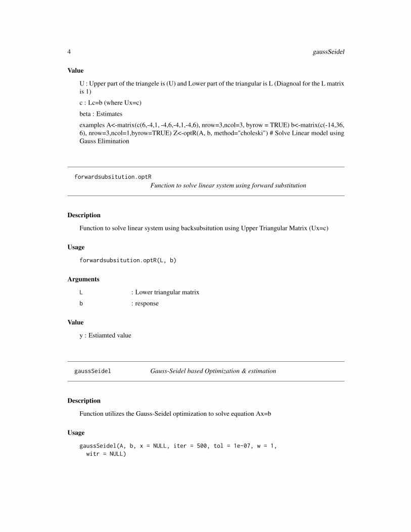
Value

U : Upper part of the triangele is (U) and Lower part of the triangular is L (Diagnoal for the L matrixis 1)

c : Lc=b (where Ux=c)

beta : Estimates

examples A<-matrix(c(6,-4,1, -4,6,-4,1,-4,6), nrow=3,ncol=3, byrow = TRUE) b<-matrix(c(-14,36,6), nrow=3,ncol=1,byrow=TRUE) Z<-optR(A, b, method="choleski") # Solve Linear model usingGauss Elimination

forwardsubsitution.optR

Function to solve linear system using forward substitution

Description

Function to solve linear system using backsubsitution using Upper Triangular Matrix (Ux=c)

Usage

forwardsubsitution.optR(L, b)

Arguments

L : Lower triangular matrix

b : response

Value

y : Estiamted value

gaussSeidel Gauss-Seidel based Optimization & estimation

Description

Function utilizes the Gauss-Seidel optimization to solve equation Ax=b

Usage

gaussSeidel(A, b, x = NULL, iter = 500, tol = 1e-07, w = 1,witr = NULL)

hatMatrix 5

Arguments

A : Input matrix

b : Response

x : Initial solutions

iter : Number of Iterations

tol : Convergence tolerance

w : Relaxation paramter used to compute weighted avg. of previous solution. w=1represent no relaxation

witr : Iteration after which relaxation parameter become active

Value

optimal : Optimal solutions

initial : initial solution

relaxationFactor : relaxation factor

Examples

A<-matrix(c(4,-1,1, -1,4,-2,1,-2,4), nrow=3,ncol=3, byrow = TRUE)b<-matrix(c(12,-1, 5), nrow=3,ncol=1,byrow=TRUE)Z<-optR(A, b, method="gaussseidel", iter=500, tol=1e-7)

hatMatrix Function determines the Hat matrix or projection matrix for given X

Description

Function hatMatrix determines the projection matrix for X from the form yhat=Hy. The projectionmatrix defines the influce of each variable on fitted value The diagonal elements of the projectionmatrix are the leverages or influence each sample has on the fitted value for that same observation.The projection matrix is evaluated with I.I.D assumtion ~N(0, 1)

Usage

hatMatrix(X, covmat = NULL)

Arguments

X : Input Matrix

covmat : covariance matrix for error, if the error are correlated for I.I.D covmat will beNULL matrix

Value

X: Projection Matrix

6 jacobian

Examples

X<-matrix(c(6,-4,1, -4,6,-4,1,-4,6), nrow=3,ncol=3, byrow = TRUE)covmat <- matrix(rnorm(3 * 3), 3, 3)H<-hatMatrix(X)H<-hatMatrix(X, covmat)diag(H)

inv.optR Invert a matrix using LU decomposition

Description

function invert a matrix A using LU decomposition such that A*inv(A)=I

Usage

inv.optR(A, tol = 1e-07)

Arguments

A : Input matrix

tol : tolerance

Value

A : Inverse of Matrix A

Examples

# Invert the matrix using LU decompositionA<-matrix(c(0.6,-0.4,1, -0.3,0.2,0.5,0.6,-1,0.5), nrow=3,ncol=3, byrow = TRUE)InvA<-inv.optR(A)

jacobian Function to evaluate jacobian matrix from functions

Description

jacobian is function to determine the jacobian matrix for function f for input x

Usage

jacobian(f, x)

LU.decompose 7

Arguments

f : function to optimize

x : Initial Solution

Value

jacobiabMatrix: Jacobian matrix

f0: Intial solution

LU.decompose LU decomposition

Description

The function decomposes matrix A into LU with L lower matrix and U as upper matrix

Usage

LU.decompose(A, tol = 1e-07)

Arguments

A : Input Matrix

tol : tolerance

Value

A : Transformed matrix with Upper part of the triangele is (U) and Lower part of the triangular is L(Diagnoal for the L matrix is 1)

Examples

A<-matrix(c(0,-1,1, -1,2,-1,2,-1,0), nrow=3,ncol=3, byrow = TRUE)Z<-optR(A, tol=1e-7, method="LU")

8 LUsplit

LU.optR Solving system of equations using LU decomposition

Description

The function solves Ax=b using LU decomposition (LUx=b). The function handles multple re-sponses

Usage

LU.optR(A, b, tol = 1e-07)

Arguments

A : Input Matrix

b : Response

tol : tolerance

Value

U : Upper part of the triangele is (U) and Lower part of the triangular is L (Diagnoal for the L matrixis 1)

c : Lc=b (where Ux=c)

beta : Estimates

Examples

A<-matrix(c(0,-1,1, -1,2,-1,2,-1,0), nrow=3,ncol=3, byrow = TRUE)b<-matrix(c(0,0, 1), nrow=3,ncol=1,byrow=TRUE)Z<-optR(A, b, method="LU")

LUsplit Function to extract Lower and Upper matrix from LU decomposition

Description

function to extract Lower and Upper matrix from LU decomposition

Usage

LUsplit(A)

Arguments

A : Input matrix

machinePrecision 9

Value

U : upper triangular matrix

L : Lower triangular matrix

Examples

A<-matrix(c(0,-1,1, -1,2,-1,2,-1,0), nrow=3,ncol=3, byrow = TRUE)Z<-optR(A, method="LU")LUsplit(Z$U)

machinePrecision Function to address machine precision error

Description

function to remove the machine precision error

Usage

machinePrecision(A)

Arguments

A : Input matrix

Value

A : return matrix

newtonRapson Function for Newton Rapson roots for given equations

Description

newtonRapson function perform optimization

Usage

newtonRapson(f, x, iteration = 30, tol = 1e-09)

Arguments

f : function to optimize

x : Initial Solution

iteration : Iterations

tol : Tolerance

10 opt.matrix.reorder

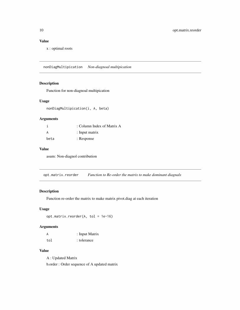
Value

x : optimal roots

nonDiagMultipication Non-diagnoal multipication

Description

Function for non-diagnoal multipication

Usage

nonDiagMultipication(i, A, beta)

Arguments

i : Column Index of Matrix A

A : Input matrix

beta : Response

Value

asum: Non-diagnol contribution

opt.matrix.reorder Function to Re-order the matrix to make dominant diagnals

Description

Function re-order the matrix to make matrix pivot.diag at each iteration

Usage

opt.matrix.reorder(A, tol = 1e-16)

Arguments

A : Input Matrix

tol : tolerance

Value

A : Updated Matrix

b.order : Order sequence of A updated matrix

optR 11

Examples

A<-matrix(c(0,-1,1, -1,2,-1,2,-1,0), nrow=3,ncol=3, byrow = TRUE)b<-matrix(c(0,0, 1), nrow=3,ncol=1,byrow=TRUE)Z<-optR(A, b, method="gauss")

optR Optimization & predictive modelling Toolsets

Description

optR function for solving linear systems using numerical approaches. Current toolbox supportsGauss Elimination, LU decomposition, Conjugate Gradiant Decent and Gauss-Sideal methods forsolving the system of form AX=b For optimization using numerical methods cgm method per-formed faster in comparision with gaussseidel. For decomposition LU is utilized for multiple re-sponses to enhance the speed of computation.

Usage

optR(x, ...)

Arguments

x : Input matrix

... : S3 method

Value

optR : Return optR class

Author(s)

PKS Prakash

Examples

# Solving equation Ax=bA<-matrix(c(6,-4,1, -4,6,-4,1,-4,6), nrow=3,ncol=3, byrow = TRUE)b<-matrix(c(-14,36, 6), nrow=3,ncol=1,byrow=TRUE)Z<-optR(A, b, method="gauss") # Solve Linear model using Gauss Elimination

# Solve Linear model using LU decomposition (Supports Multi-response)Z<-optR(A, b, method="LU")

# Solve the matrix using Gauss Elimination (1, -1, 2)A<-matrix(c(2,-2,6, -2,4,3,-1,8,4), nrow=3,ncol=3, byrow = TRUE)b<-matrix(c(16,0, -1), nrow=3,ncol=1,byrow=TRUE)Z<-optR(A, b, method="gauss") # Solve Linear model using Gauss Elimination

12 optR.default

require(utils)set.seed(129)n <- 10 ; p <- 4X <- matrix(rnorm(n * p), n, p) # no intercept!y <- rnorm(n)Z<-optR(X, y, method="cgm")

optR.backsubsitution Function to solve linear system using backsubsitution

Description

Function to solve linear system using backsubsitution using Upper Triangular Matrix (Ux=c)

Usage

## S3 method for class 'backsubsitution'optR(U, c)

Arguments

U : Upper triangular matrix

c : response

Value

beta : Estiamted value

optR.default Optimization & predictive modelling Toolsets

Description

soptR is the default function for optimization

Usage

## Default S3 method:optR(x, y = NULL, weights = NULL, method = c("gauss",

"LU", "gaussseidel", "cgm", "choleski"), iter = 500, tol = 1e-07,keep.data = TRUE, ...)

optR.fit 13

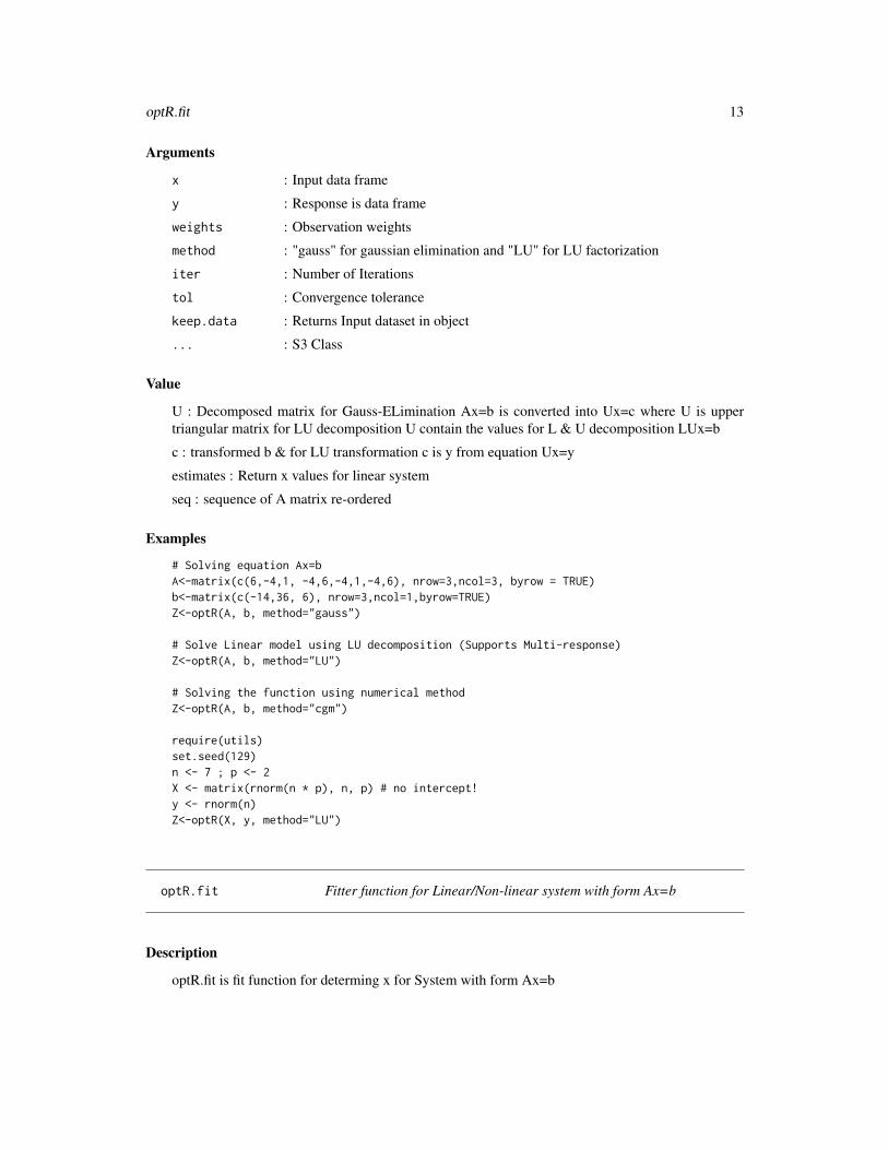
Arguments

x : Input data frame

y : Response is data frame

weights : Observation weights

method : "gauss" for gaussian elimination and "LU" for LU factorization

iter : Number of Iterations

tol : Convergence tolerance

keep.data : Returns Input dataset in object

... : S3 Class

Value

U : Decomposed matrix for Gauss-ELimination Ax=b is converted into Ux=c where U is uppertriangular matrix for LU decomposition U contain the values for L & U decomposition LUx=b

c : transformed b & for LU transformation c is y from equation Ux=y

estimates : Return x values for linear system

seq : sequence of A matrix re-ordered

Examples

# Solving equation Ax=bA<-matrix(c(6,-4,1, -4,6,-4,1,-4,6), nrow=3,ncol=3, byrow = TRUE)b<-matrix(c(-14,36, 6), nrow=3,ncol=1,byrow=TRUE)Z<-optR(A, b, method="gauss")

# Solve Linear model using LU decomposition (Supports Multi-response)Z<-optR(A, b, method="LU")

# Solving the function using numerical methodZ<-optR(A, b, method="cgm")

require(utils)set.seed(129)n <- 7 ; p <- 2X <- matrix(rnorm(n * p), n, p) # no intercept!y <- rnorm(n)Z<-optR(X, y, method="LU")

optR.fit Fitter function for Linear/Non-linear system with form Ax=b

Description

optR.fit is fit function for determing x for System with form Ax=b

14 optR.formula

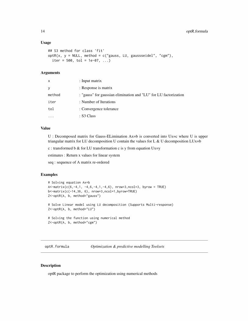
Usage

## S3 method for class 'fit'optR(x, y = NULL, method = c("gauss, LU, gaussseidel", "cgm"),iter = 500, tol = 1e-07, ...)

Arguments

x : Input matrix

y : Response is matrix

method : "gauss" for gaussian elimination and "LU" for LU factorization

iter : Number of Iterations

tol : Convergence tolerance

... : S3 Class

Value

U : Decomposed matrix for Gauss-ELimination Ax=b is converted into Ux=c where U is uppertriangular matrix for LU decomposition U contain the values for L & U decomposition LUx=b

c : transformed b & for LU transformation c is y from equation Ux=y

estimates : Return x values for linear system

seq : sequence of A matrix re-ordered

Examples

# Solving equation Ax=bA<-matrix(c(6,-4,1, -4,6,-4,1,-4,6), nrow=3,ncol=3, byrow = TRUE)b<-matrix(c(-14,36, 6), nrow=3,ncol=1,byrow=TRUE)Z<-optR(A, b, method="gauss")

# Solve Linear model using LU decomposition (Supports Multi-response)Z<-optR(A, b, method="LU")

# Solving the function using numerical methodZ<-optR(A, b, method="cgm")

optR.formula Optimization & predictive modelling Toolsets

Description

optR package to perform the optimization using numerical methods

optR.formula 15

Usage

## S3 method for class 'formula'optR(formula, data = list(), weights = NULL,method = c("gauss, LU, gaussseidel", "cgm", "choleski"), iter = 500,tol = 1e-07, keep.data = TRUE, contrasts = NULL, ...)

Arguments

formula : formula to build model

data : data used to build model

weights : Observation weights

method : "gauss" for gaussian elimination and "LU" for LU factorization

iter : Number of Iterations

tol : Convergence tolerance

keep.data : If TRUE returns input data

contrasts : Data frame contract values

... : S3 Class

Value

U : Decomposed matrix for Gauss-ELimination Ax=b is converted into Ux=c where U is uppertriangular matrix for LU decomposition U contain the values for L & U decomposition LUx=b

c : transformed b & for LU transformation c is y from equation Ux=y

estimates : Return x values for linear system

Author(s)

PKS Prakash

Examples

# Solving equation Ax=bb<-matrix(c(-14,36, 6), nrow=3,ncol=1,byrow=TRUE)A<-matrix(c(6,-4,1, -4,6,-4,1,-4,6), nrow=3,ncol=3, byrow = TRUE)Z<-optR(b~A-1, method="gauss") # -1 to remove the constant vector

Z<-optR(b~A-1, method="LU") # -1 to remove the constant vector

require(utils)set.seed(129)n <- 10 ; p <- 4X <- matrix(rnorm(n * p), n, p) # no intercept!y <- rnorm(n)data<-cbind(X, y)colnames(data)<-c("var1", "var2", "var3", "var4", "y")Z<-optR(y~var1+var2+var3+var4+var1*var2-1, data=data.frame(data), method="cgm")

16 optR.multiplyfactor

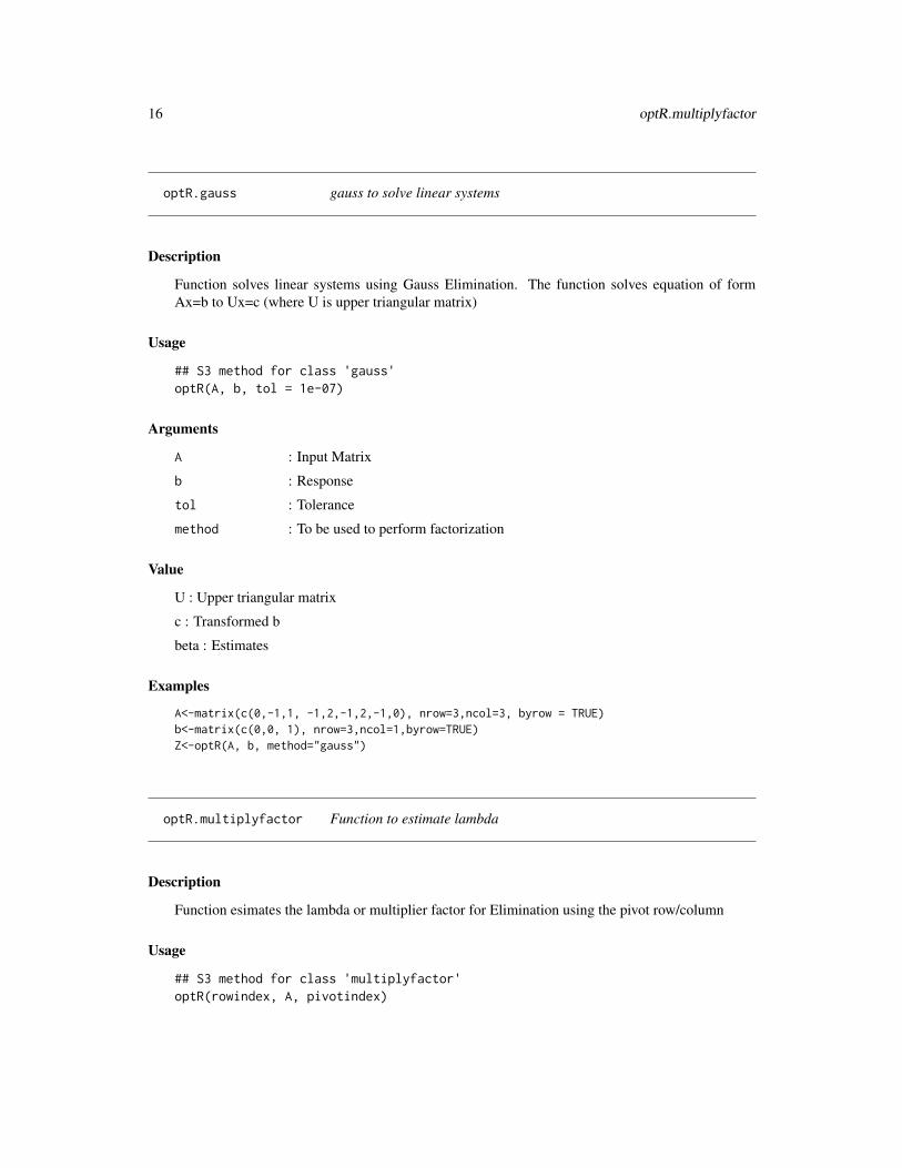
optR.gauss gauss to solve linear systems

Description

Function solves linear systems using Gauss Elimination. The function solves equation of formAx=b to Ux=c (where U is upper triangular matrix)

Usage

## S3 method for class 'gauss'optR(A, b, tol = 1e-07)

Arguments

A : Input Matrix

b : Response

tol : Tolerance

method : To be used to perform factorization

Value

U : Upper triangular matrix

c : Transformed b

beta : Estimates

Examples

A<-matrix(c(0,-1,1, -1,2,-1,2,-1,0), nrow=3,ncol=3, byrow = TRUE)b<-matrix(c(0,0, 1), nrow=3,ncol=1,byrow=TRUE)Z<-optR(A, b, method="gauss")

optR.multiplyfactor Function to estimate lambda

Description

Function esimates the lambda or multiplier factor for Elimination using the pivot row/column

Usage

## S3 method for class 'multiplyfactor'optR(rowindex, A, pivotindex)

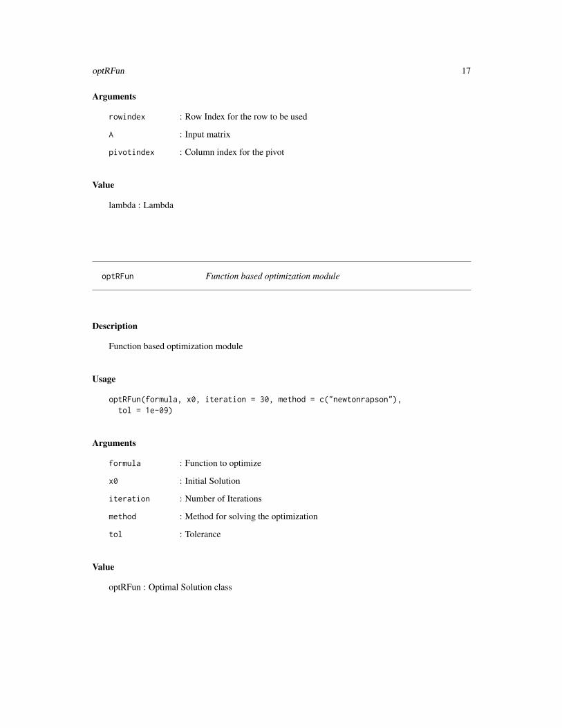
optRFun 17

Arguments

rowindex : Row Index for the row to be used

A : Input matrix

pivotindex : Column index for the pivot

Value

lambda : Lambda

optRFun Function based optimization module

Description

Function based optimization module

Usage

optRFun(formula, x0, iteration = 30, method = c("newtonrapson"),tol = 1e-09)

Arguments

formula : Function to optimize

x0 : Initial Solution

iteration : Number of Iterations

method : Method for solving the optimization

tol : Tolerance

Value

optRFun : Optimal Solution class

18 predict.optR

optRFun.newtonRapson Function based optimization module

Description

Newton Rapshon based optimization

Usage

optRFun.newtonRapson(formula, x0, iteration = 30, tol = 1e-09)

Arguments

formula : Function to optimizex0 : Initial Solutioniteration : Number of Iterationstol : Tolerance

Value

optRFun : Optimal Solution

predict.optR Prediction function based on optR class

Description

Function for making predictions using OptR class

Usage

## S3 method for class 'optR'predict(object, newdata, na.action = na.pass, ...)

Arguments

object : optR class fitted objectnewdata : data for predictionna.action : action for missing values... : S3 class

Value

fitted.val : Predicted values

terms : terms used for fitting

print.optR 19

print.optR print coefficients for optR class

Description

optR is the default function for optimization

Usage

## S3 method for class 'optR'print(x, ...)

Arguments

x : Input of optR class

... : S3 class

Examples

# Solving equation Ax=bA<-matrix(c(6,-4,1, -4,6,-4,1,-4,6), nrow=3,ncol=3, byrow = TRUE)b<-matrix(c(-14,36, 6), nrow=3,ncol=1,byrow=TRUE)Z<-optR(A, b, method="gauss")print(Z)

summary.optR Generate Summary for optR class

Description

summary function generates the summary for the optR class

Usage

## S3 method for class 'optR'summary(object, ...)

Arguments

object : Input of optR class

... : S3 method

20 summary.optR

Examples

# Solving equation Ax=bA<-matrix(c(6,-4,1, -4,6,-4,1,-4,6), nrow=3,ncol=3, byrow = TRUE)b<-matrix(c(-14,36, 6), nrow=3,ncol=1,byrow=TRUE)Z<-optR(A, b, method="cgm")summary(Z)

Index

cgm, 2choleskiDecomposition, 3choleskilm, 3

forwardsubsitution.optR, 4

gaussSeidel, 4

hatMatrix, 5

inv.optR, 6

jacobian, 6

LU.decompose, 7LU.optR, 8LUsplit, 8

machinePrecision, 9

newtonRapson, 9nonDiagMultipication, 10

opt.matrix.reorder, 10optR, 11optR.backsubsitution, 12optR.default, 12optR.fit, 13optR.formula, 14optR.gauss, 16optR.multiplyfactor, 16optRFun, 17optRFun.newtonRapson, 18

predict.optR, 18print.optR, 19

summary.optR, 19

21