Package ‘R0’ - The Comprehensive R Archive Network · Package ‘R0’ May 21, 2015 Type...

Package ‘R0’May 21, 2015

Type Package

Title Estimation of R0 and Real-Time Reproduction Number fromEpidemics

Version 1.2-6

Date 2015-05-21

Author Pierre-Yves Boelle, Thomas Obadia

Maintainer Thomas Obadia <[email protected]>

Depends R (>= 2.13.0), MASS

Description Estimation of reproduction numbers for disease outbreak, based onincidence data. The R0 package implements several documented methods. It istherefore possible to compare estimations according to the methods used.Depending on the methods requested by user, basic reproduction number(commonly denoted as R0) or real-time reproduction number (referred to asR(t)) is computed, along with a 95% Confidence Interval. Plotting outputswill give different graphs depending on the methods requested : basicreproductive number estimations will only show the epidemic curve(collected data) and an adjusted model, whereas real-time methods will alsoshow the R(t) variations throughout the outbreak time period. Sensitivityanalysis tools are also provided, and allow for investigating effects ofvarying Generation Time distribution or time window on estimates.

License GPL (>= 2)

LazyLoad yes

NeedsCompilation no

Repository CRAN

Date/Publication 2015-05-21 19:34:12

R topics documented:R0-package . . . . . . . . . . . . . . . . . . . . . . . . . . . . . . . . . . . . . . . . . 2check.incid . . . . . . . . . . . . . . . . . . . . . . . . . . . . . . . . . . . . . . . . . 3est.GT . . . . . . . . . . . . . . . . . . . . . . . . . . . . . . . . . . . . . . . . . . . . 4est.R0.AR . . . . . . . . . . . . . . . . . . . . . . . . . . . . . . . . . . . . . . . . . . 6

1

2 R0-package

est.R0.EG . . . . . . . . . . . . . . . . . . . . . . . . . . . . . . . . . . . . . . . . . . 8est.R0.ML . . . . . . . . . . . . . . . . . . . . . . . . . . . . . . . . . . . . . . . . . . 10est.R0.SB . . . . . . . . . . . . . . . . . . . . . . . . . . . . . . . . . . . . . . . . . . 12est.R0.TD . . . . . . . . . . . . . . . . . . . . . . . . . . . . . . . . . . . . . . . . . . 14estimate.R . . . . . . . . . . . . . . . . . . . . . . . . . . . . . . . . . . . . . . . . . . 16generation.time . . . . . . . . . . . . . . . . . . . . . . . . . . . . . . . . . . . . . . . 19Germany.1918 . . . . . . . . . . . . . . . . . . . . . . . . . . . . . . . . . . . . . . . . 20GT.chld.hsld . . . . . . . . . . . . . . . . . . . . . . . . . . . . . . . . . . . . . . . . . 21H1N1.serial.interval . . . . . . . . . . . . . . . . . . . . . . . . . . . . . . . . . . . . . 22impute.incid . . . . . . . . . . . . . . . . . . . . . . . . . . . . . . . . . . . . . . . . . 22plot.R0.S . . . . . . . . . . . . . . . . . . . . . . . . . . . . . . . . . . . . . . . . . . 23plotfit . . . . . . . . . . . . . . . . . . . . . . . . . . . . . . . . . . . . . . . . . . . . 24sa.GT . . . . . . . . . . . . . . . . . . . . . . . . . . . . . . . . . . . . . . . . . . . . 25sa.time . . . . . . . . . . . . . . . . . . . . . . . . . . . . . . . . . . . . . . . . . . . . 27sensitivity.analysis . . . . . . . . . . . . . . . . . . . . . . . . . . . . . . . . . . . . . 29sim.epid . . . . . . . . . . . . . . . . . . . . . . . . . . . . . . . . . . . . . . . . . . . 31sim.epid.indiv . . . . . . . . . . . . . . . . . . . . . . . . . . . . . . . . . . . . . . . . 32smooth.Rt . . . . . . . . . . . . . . . . . . . . . . . . . . . . . . . . . . . . . . . . . . 33

Index 36

R0-package Estimation of R0 and Real-Time Reproduction Number from Epi-demics

Description

Estimation of reproduction numbers for disease outbreak, based on incidence data. The R0 packageimplements several documented methods. It is therefore possible to compare estimations accordingto the methods used. Depending on the methods requested by user, basic reproduction number(commonly denoted as R0) or real-time reproduction number (referred to as R(t)) is computed,along with a 95% Confidence Interval. Plotting outputs will give different graphs depending onthe methods requested : basic reproductive number estimations will only show the epidemic curve(collected data) and an adjusted model, whereas real-time methods will also show the R(t) variationsthroughout the outbreak time period. Sensitivity analysis tools are also provided, and allow forinvestigating effects of varying Generation Time distribution or time window on estimates.

Details

Package: R0Type: PackageTitle: Estimation of R0 and Real-Time Reproduction Number from EpidemicsVersion: 1.2-6Date: 2015-05-21Author: Pierre-Yves Boelle, Thomas ObadiaMaintainer: Thomas Obadia <[email protected]>Depends: R (>= 2.13.0), MASSLicense: GPL (>= 2)

check.incid 3

LazyLoad: yes

Author(s)

Pierre-Yves Boelle, Thomas Obadia

check.incid Check incid in the input

Description

Checks incid in the input. For internal use only.

Usage

check.incid(incid, t = NULL, date.first.obs = NULL, time.step = 1)

Arguments

incid An object (vector, data.frame, list) storing incidence

t An optional vector of dates.

date.first.obs Optional date of first observation, if t not specified

time.step Optional. If date of first observation is specified, number of day between eachincidence observation

Details

For internal use. Called by estimation methods to format incidence input.

check.incid handles everything related to incidence content integrity. It is designed to generate anoutput which comply with estimation functions requirements. Epidemic data can be provided asan epitools object (see below) or as vectors (incidence, dates, or both). When dates are provided,they can be in a separate t vector, or computed with the first value and a time step. In the end,the function returns a list with "epid" and "t" values. If you plan on using estimation functions ontheir own (and not throught est.R0), be aware that any incorrect input format will result in erraticbehavior and/or crash.

Object incid is either a list or data.frame. Expect item/column "$dates"" and/or "$stratum3". Thisis expected to work with objects created by epitools package (tested with v0.5-6).

Epicurve.dates returns (among other things) a list with $dates object. This list gives incidence perday. Other epicurve methods return $dates along with a $<time_period> object and a $stratum3,which contains respectively daily incidence data agregated by the given time period, and the samedata with colnames that comply with R standard time notation.

4 est.GT

E.g.: epicurve.weeks returns $dates, $weeks and $stratum3. $stratum3 object is a list of dates(correct syntax), where each date is repeated to reflect the incidence value at this time.

Incidence data should not contain negative or missing values.

Incidence data and time vector should have the same length.

Value

A list with components incid and t.

Author(s)


Examples

#Loading packagelibrary(R0)

## Data is taken from the paper by Nishiura for key transmission parameters of an institutional## outbreak during 1918 influenza pandemic in Germanydata(Germany.1918)Germany.1918

## check.incid will extract names from the vector and coerce them as datescheck.incid(Germany.1918)

## Had Germany.1918 not have names() set, output would have been with index dates## To force such an output, we here impose t=1:126.## Erasing names(Germany.1918) would have produced the same## If so, then the epid$t vector returned will be replacement values.check.incid(Germany.1918, t=1:126)

## You can also choose not to provide a complete date vector, but to only## indicated the first day of the observation, and the number of days between each## observation. In this example we will assume a time step of 7 days.check.incid(Germany.1918, date.first.obs="1918-01-01", time.step=7)

## Finally, if no names() are available for the dataset and date.first.obs is not provided,## setting time.step to any integer value will generate a t vector starting## from 1 and incrementing by the time.step parameter.

est.GT Find the best-fitting GT distribution for a series of serial interval

Description

Find the best-fitting GT distribution for a series of serial interval

est.GT 5

Usage

est.GT(infector.onset.dates = NULL, infectee.onset.dates = NULL,serial.interval = NULL, request.plot = FALSE, ...)

Arguments

infector.onset.dates

Vector of dates for infector symptoms onset.infectee.onset.dates

Vector of dates for infectee symptoms onset.serial.interval

Vector of reported serial interval.

request.plot Should data adjsument be displayed at the end?

... Parameters passed to other functions (useful for hidden parameters of generation.time)

Details

Generation Time distribution can be estimated by two inputs methods. User can either provide twovectors of dates or a unique vector of reported serial intervals. If two vectors are provided, bothonset.dates vectors should be of same length. Element i is the onset date for individual i. Thismeans that infector k (symptoms on day infector.onset.dates[k]) infected infectee k (symptoms onday infectee.onset.dates[k]) If only serial.interval is provided, each record is assumed to be the timeelapsed between each pair of infector and infectee.

When request.plot is set to TRUE, a graphical output provides standardized histogram of observeddata along with the best-fitting adjusted model.

Value

A R0.GT object that complies with generation.time distribution requirements of the R0 package

Author(s)


Examples


# Data taken from traced cases of H1N1 viruses.data(H1N1.serial.interval)est.GT(serial.interval=H1N1.serial.interval)

## Best fitting GT distribution is a gamma distribution with mean = 3.039437 and sd = 1.676551 .## Discretized Generation Time distribution## mean: 3.070303 , sd: 1.676531## [1] 0.0000000000 0.1621208802 0.2704857362 0.2358751176 0.1561845680 0.0888997193 0.0459909903## 0.0222778094 0.0102848887 0.0045773285 0.0019791984 0.0008360608 0.0003464431 0.0001412594

6 est.R0.AR

# The same result can be achieved with two vectors of dates of onset.# Here we use the same data, but trick the function into thinking onset dates are all "0".data(H1N1.serial.interval)est.GT(infector.onset.dates=rep(0,length(H1N1.serial.interval)),

infectee.onset.dates=H1N1.serial.interval)

est.R0.AR Estimate R0 from attack rate of an epidemic

Description

Estimate R0 from attack rate of an epidemic.

Usage

est.R0.AR(AR = NULL, incid = NULL, pop.size = NULL, S0 = 1, checked = FALSE,...)

Arguments

AR Attack rate as a percentage from total population

incid Sum of incident cases, possibly in the form of a vector of counts.

pop.size Population size in which the incident cases were observed.

S0 Initial proportion of the population considered susceptible.

checked Internal flag used to check whether integrity checks were ran or not.

... parameters passed to inner functions

Details

For internal use. Called by est.R0.

In the simple SIR model, the relation between R0 and the Attack Rate is in the form R0 = −ln((1−AR)/S0)/(AR− (1− S0)).

If the population size is provided, the variance of R0 is estimated using the delta method. Thehypothesis are that of homogeneous mixing, no more transmission (epidemic ended), no change intransmission or interventions during the epidemic. This estimate may be correct in closed popula-tions, and may be less valid in other cases.

The correction for incomplete susceptibility is based on the SIR model equations.

CI is computed for the attack rate considering the population size (CI(AR) = AR + / − 1.96 ∗sqrt(AR∗ (1−AR)/n)), and so the CI for the reproduction number is computed with this extremevalues.

est.R0.AR 7

Value

A list with components:

epid The vector of incidence, after being correctly formated by check.incid. Usedonly by plot.fit.

R The estimate of the reproduction ratio.

conf.int The 95% confidence interval for the R estimate.


begin.nb First date of incidence record. Used only by plot.fit.

end.nb Last date of incidence record. Used only by plot.fit.

method Method used for the estimation.

method.code Internal code used to designate method.

Note

This is the implementation of the formula by Dietz (1993).

Author(s)


References

Dietz, K. "The Estimation of the Basic Reproduction Number for Infectious Diseases." StatisticalMethods in Medical Research 2, no. 1 (March 1, 1993): 23-41.

Examples


## Woodall reported an attack rate of 0.31 in a population of 1732 during## the 1957 H2N2 influenza pandemic ('Age and Asian Influenza, 1957', BMJ, 1958)

est.R0.AR(pop.size=1732, AR=0.31)# Reproduction number estimate using Attack Rate method# R : 1.19698[ 1.179606 , 1.215077 ]

est.R0.AR(AR=0.31)# Reproduction number estimate using Attack Rate method.# R : 1.19698

est.R0.AR(pop.size=1732, incid=31)# Reproduction number estimate using Attack Rate method# R : 1.009057[ 1.005873 , 1.012269 ]

est.R0.AR(pop.size=1732, incid=c(2,3,4,7,4,2,4,5))# Reproduction number estimate using Attack Rate method# R : 1.009057[ 1.005873 , 1.012269 ]

8 est.R0.EG

est.R0.AR(pop.size=1732, incid=c(2,3,0,7,4,2,0,5))# Reproduction number estimate using Attack Rate method# R : 1.006699[ 1.003965 , 1.009453 ]

est.R0.EG Estimate R from exponential growth rate

Description

Estimate R from exponential growth rate.

Usage

est.R0.EG(epid, GT, t = NULL, begin = NULL, end = NULL, date.first.obs = NULL,time.step = 1, reg.met = "poisson", checked = FALSE, ...)

Arguments

epid object containing epidemic curve data. see Details.

GT generation time distribution

t Vector of dates at which incidence was calculated

begin At what time estimation begins

end Time at which to end computation



reg.met Regression method used. Default is "poisson" (for GLM), but can be forced to"linear".



Details


method "poisson" uses Poisson regression of incidence. method "linear" uses linear regression oflog(incidence)

CI is computed from the 1/M(-r) formula using bounds on r from the Poisson regression.

est.R0.EG 9

Value




r Exponential growth rate of the epidemic.

conf.int.r Confidence interval of the exponential growth rate of the epidemic.

Rsquared The deviance R-squared measure for the considered dates and model.

epid object containing epidemic curve data. see Details.


data.name Name of the data used in the fit.


begin.nb The number of the first day used in the fit.


end.nb The number of the las day used for the fit.

fit Method used for fitting.

pred Prediction on the period used for the fit.

method Method for estimation.


Note

This is the implementation of the method provided by Wallinga & Lipsitch (2007).

Author(s)


References

Wallinga, J., and M. Lipsitch. "How Generation Intervals Shape the Relationship Between GrowthRates and Reproductive Numbers." Proceedings of the Royal Society B: Biological Sciences 274,no. 1609 (2007): 599.

Examples


## Data is taken from the paper by Nishiura for key transmission parameters of an institutional## outbreak during 1918 influenza pandemic in Germany)

data(Germany.1918)mGT<-generation.time("gamma", c(3, 1.5))

10 est.R0.ML

est.R0.EG(Germany.1918, mGT, begin=1, end=27)## Reproduction number estimate using Exponential Growth## R : 1.525895[ 1.494984 , 1.557779 ]

est.R0.ML Estimate the reproduction number by maximum likelihood

Description

Estimate the reproduction number by maximum likelihood

Usage

est.R0.ML(epid, GT, import = NULL, t = NULL, begin = NULL, end = NULL,date.first.obs = NULL, time.step = 1, range = c(0.01, 50),unknown.GT = FALSE, impute.values = FALSE, checked = FALSE,...)

Arguments

epid the epidemic curve


import Vector of imported cases.

t Vector of dates at which incidence was calculated





range Range in which the maximum must be looked for

unknown.GT When GT distribution is unknown, it is estimated jointly. See details.

impute.values Boolean value. If TRUE, will impute unobserved cases at the beginning of theepidemic to correct for censored data



Details


White & Pagano (2009) detail two maximum likelihood methods for estimatig the reproductionratio. The first (and used by default in this package) assumes that the serial interval distirbutionis known, and subsequently the likelihood is only maximised depending on the value of R. Thesecond method can be used if the serial interval distribution is unknown: in that case, the generationtime is set to follow a Gamma distribution with two parameters (size, shape), and the optimization

est.R0.ML 11

routine finds the values of R, size and shape that maximize the likelihood. However, the epidemiccurve must be long enough to account for a whole generation. The authors showed that this isachieved when the cumulated amount of incident cases reaches 150. When using this method, theflag unknown.GT must be set to TRUE. GT must still be provided with a R0.GT-class object, howeverits mean and sd will be recycled as starting value for the optimization routine.

The principle of the methods described by White & all is to compute the expected number of casesin the future, and optimise to get R using a Poisson distribution.

CI is achieved by profiling the likelihood.

Value





epid.orig Original epidemic data.



begin.nb The number of the first day used in the fit.


end.nb The number of the las day used for the fit.

pred Prediction on the period used for the fit.

Rsquared Correlation coefficient between predicted curve (by fit.epid) and observed epi-demic curve.

call Call used for the function.

method Method used for fitting.


Note

This is the implementation of the method provided by White & Pagano (2009).

Author(s)


References

White, L.F., J. Wallinga, L. Finelli, C. Reed, S. Riley, M. Lipsitch, and M. Pagano. "Estimationof the Reproductive Number and the Serial Interval in Early Phase of the 2009 Influenza A/H1N1Pandemic in the USA." Influenza and Other Respiratory Viruses 3, no. 6 (2009): 267-276.

12 est.R0.SB

Examples


## Data is taken from paper by Nishiura for key transmission parameters of an institutional## outbreak during the 1918 influenza pandemic in Germany)

data(Germany.1918)mGT<-generation.time("gamma", c(2.45, 1.38))est.R0.ML(Germany.1918, mGT, begin=1, end=27, range=c(0.01,50))# Reproduction number estimate using Maximum Likelihood method.# R : 1.307222[ 1.236913 , 1.380156 ]

res=est.R0.ML(Germany.1918, mGT, begin=1, end=27, range=c(0.01,50))plot(res)

## no change in R with varying range## (dates here are the same index as before. Just to illustrate different use)est.R0.ML(Germany.1918, mGT, begin="1918-09-29", end="1918-10-25", range=c(0.01,100))# Reproduction number estimate using Maximum Likelihood method.# R : 1.307249[ 1.236913 , 1.380185 ]

est.R0.SB Estimate the time dependent reproduction number using a Bayesianapproach

Description

Estimate the time dependent reproduction number using a Bayesian approach. All known data areused as a prior for next iteration (see Details).

Usage

est.R0.SB(epid, GT, t = NULL, begin = NULL, end = NULL, date.first.obs = NULL,time.step = 1, force.prior = FALSE, checked = FALSE, ...)

Arguments



t Time at which epidemic was observed

begin At what time estimation begins. Just there for "plot" purposes, not actually used

end At what time estimation ends. Just there for "plot" purposes, not actually used



est.R0.SB 13

force.prior Set to any custom value to force the initial prior as a uniform distribution on[0;value]



Details


Initial prior is an unbiased uniform distribution for R, between 0 and the maximum of incid(t+1)- incid(t). For each subsequent iteration, a new distribution is computed for R, using the previousoutput as new prior.

CI is achieved by a cumulated sum of the R posterior distribution, and corresponds to the 2.5% and97.5% thresholds

Value


R vector of R values.

conf.int 95% confidence interval for estimates.

proba.Rt A list with successive distribution for R throughout the outbreak.



begin At what time estimation begins. Just there for "plot" purposes, not actually used

begin.nb Index of begin date for the fit.

end At what time estimation ends. Just there for "plot" purposes, not actually used

end.nb Index of end date for the fit.

pred Predictive curve based on most-likely R value.

data.name Name of the data used in the fit.

call Complete call used to generate results.

method Method for estimation.


Note

This is the implementation of the method provided by Bettencourt & Ribeiro (2008).

Author(s)


References

Bettencourt, L.M.A., and R.M. Ribeiro. "Real Time Bayesian Estimation of the Epidemic Potentialof Emerging Infectious Diseases." PLoS One 3, no. 5 (2008): e2185.

14 est.R0.TD

Examples



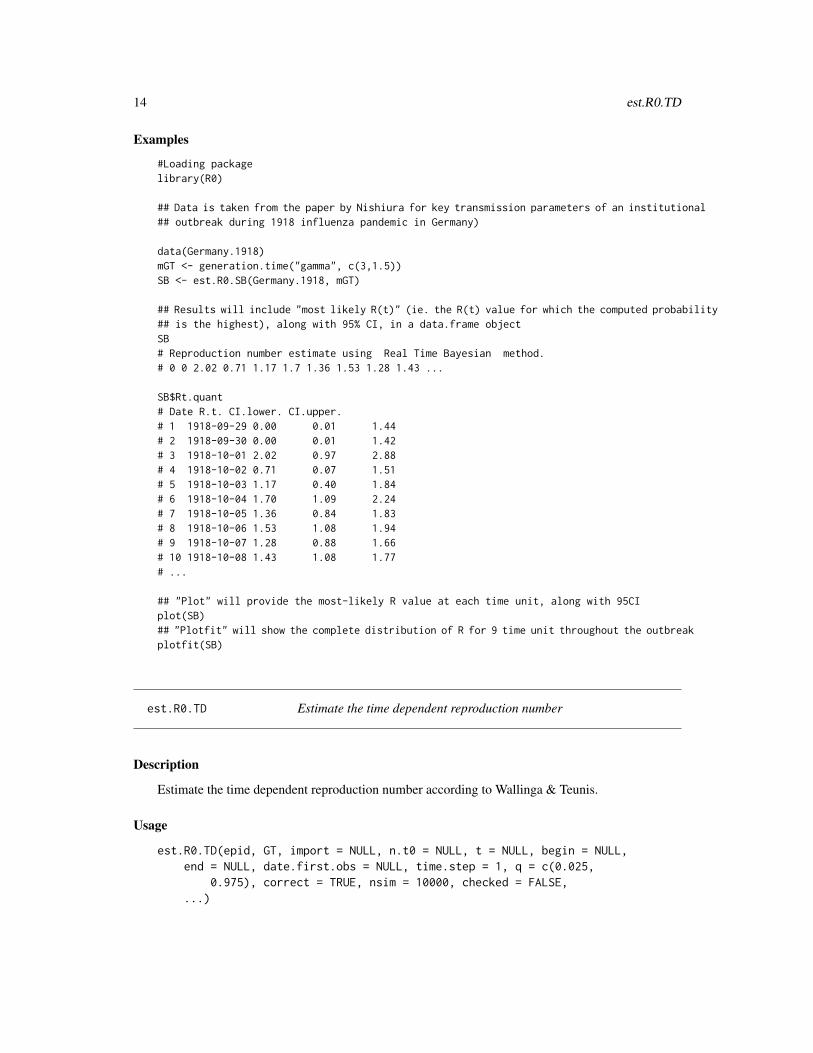
data(Germany.1918)mGT <- generation.time("gamma", c(3,1.5))SB <- est.R0.SB(Germany.1918, mGT)

## Results will include "most likely R(t)" (ie. the R(t) value for which the computed probability## is the highest), along with 95% CI, in a data.frame objectSB# Reproduction number estimate using Real Time Bayesian method.# 0 0 2.02 0.71 1.17 1.7 1.36 1.53 1.28 1.43 ...

SB$Rt.quant# Date R.t. CI.lower. CI.upper.# 1 1918-09-29 0.00 0.01 1.44# 2 1918-09-30 0.00 0.01 1.42# 3 1918-10-01 2.02 0.97 2.88# 4 1918-10-02 0.71 0.07 1.51# 5 1918-10-03 1.17 0.40 1.84# 6 1918-10-04 1.70 1.09 2.24# 7 1918-10-05 1.36 0.84 1.83# 8 1918-10-06 1.53 1.08 1.94# 9 1918-10-07 1.28 0.88 1.66# 10 1918-10-08 1.43 1.08 1.77# ...

## "Plot" will provide the most-likely R value at each time unit, along with 95CIplot(SB)## "Plotfit" will show the complete distribution of R for 9 time unit throughout the outbreakplotfit(SB)

est.R0.TD Estimate the time dependent reproduction number

Description

Estimate the time dependent reproduction number according to Wallinga & Teunis.

Usage

est.R0.TD(epid, GT, import = NULL, n.t0 = NULL, t = NULL, begin = NULL,end = NULL, date.first.obs = NULL, time.step = 1, q = c(0.025,

0.975), correct = TRUE, nsim = 10000, checked = FALSE,...)

est.R0.TD 15

Arguments

epid epidemic curve.GT generation time distribution.import Vector of imported cases.n.t0 Number of cases at time 0.t Vector of dates at which incidence was measured.begin At what time estimation begins. Just here for "plot" purposes, not actually usedend At what time estimation ends. Just here for "plot" purposes, not actually useddate.first.obs Optional date of first observation, if t not specifiedtime.step Optional. If date of first observation is specified, number of day between each

incidence observation.q Quantiles for R(t). By default, 5% and 95%correct Correction for cases not yet observed (real time).nsim Number of simulations to be run to compute quantiles for R(t)checked Internal flag used to check whether integrity checks were ran or not.... parameters passed to inner functions

Details


CI is computed by multinomial simulations at each time step with the expected value of R.

Value


R vector of R values.conf.int 95% confidence interval for estimates.P Matrix of who infected whom.p Probability of who infected whom (values achieved by normalizing P matrix).GT generation time distribution.epid epidemic curve.import Vector of imported cases.pred Theoretical epidemic data, computed with estimated values of R.begin At what time estimation begins. Just here for "plot" purposes, not actually usedbegin.nb The number of the first day used in the fit.end At what time estimation ends. Just here for "plot" purposes, not actually usedend.nb The number of the las day used for the fit.data.name Name of the data used in the fit.call Call used for the function.method Method for estimation.method.code Internal code used to designate method.

16 estimate.R

Note

This is the implementation of the method provided by Wallinga & Teunis (2004). Correction forestimation in real time is implemented as in Cauchemez et al, AJE (2006).

If imported cases are provided, they are counted in addition to autonomous cases. The final plotwill show overall incidence.

Author(s)


References

Wallinga, J., and P. Teunis. "Different Epidemic Curves for Severe Acute Respiratory Syndrome Re-veal Similar Impacts of Control Measures." American Journal of Epidemiology 160, no. 6 (2004):509.

Examples



data(Germany.1918)mGT<-generation.time("gamma", c(3, 1.5))TD <- est.R0.TD(Germany.1918, mGT, begin=1, end=126, nsim=100)# Warning messages:# 1: In est.R0.TD(Germany.1918, mGT) : Simulations may take several minutes.# 2: In est.R0.TD(Germany.1918, mGT) : Using initial incidence as initial number of cases.TD# Reproduction number estimate using Time-Dependent method.# 2.322239 2.272013 1.998474 1.843703 2.019297 1.867488 1.644993 1.553265 1.553317 1.601317 ...

## An interesting way to look at these results is to agregate initial data by longest time unit,## such as weekly incidence. This gives a global overview of the epidemic.TD.weekly <- smooth.Rt(TD, 7)TD.weekly# Reproduction number estimate using Time-Dependant method.# 1.878424 1.580976 1.356918 1.131633 0.9615463 0.8118902 0.8045254 0.8395747 0.8542518 0.8258094..plot(TD.weekly)

estimate.R Estimate R0 for one incidence dataset using several methods

Description

Estimate R0 for one incidence dataset using several methods.

estimate.R 17

Usage

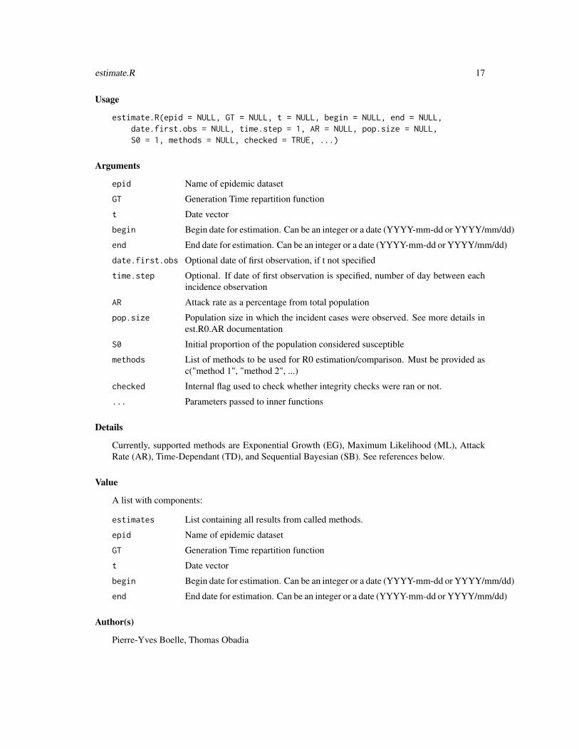
estimate.R(epid = NULL, GT = NULL, t = NULL, begin = NULL, end = NULL,date.first.obs = NULL, time.step = 1, AR = NULL, pop.size = NULL,S0 = 1, methods = NULL, checked = TRUE, ...)

Arguments

epid Name of epidemic dataset

GT Generation Time repartition function

t Date vector

begin Begin date for estimation. Can be an integer or a date (YYYY-mm-dd or YYYY/mm/dd)

end End date for estimation. Can be an integer or a date (YYYY-mm-dd or YYYY/mm/dd)




pop.size Population size in which the incident cases were observed. See more details inest.R0.AR documentation

S0 Initial proportion of the population considered susceptible

methods List of methods to be used for R0 estimation/comparison. Must be provided asc("method 1", "method 2", ...)


... Parameters passed to inner functions

Details

Currently, supported methods are Exponential Growth (EG), Maximum Likelihood (ML), AttackRate (AR), Time-Dependant (TD), and Sequential Bayesian (SB). See references below.

Value


estimates List containing all results from called methods.

epid Name of epidemic dataset

GT Generation Time repartition function

t Date vector

begin Begin date for estimation. Can be an integer or a date (YYYY-mm-dd or YYYY/mm/dd)

end End date for estimation. Can be an integer or a date (YYYY-mm-dd or YYYY/mm/dd)

Author(s)


18 estimate.R

References

est.R0.EG: Wallinga, J., and M. Lipsitch. "How Generation Intervals Shape the Relationship Be-tween Growth Rates and Reproductive Numbers." Proceedings of the Royal Society B: BiologicalSciences 274, no. 1609 (2007): 599.

est.R0.ML: White, L.F., J. Wallinga, L. Finelli, C. Reed, S. Riley, M. Lipsitch, and M. Pagano."Estimation of the Reproductive Number and the Serial Interval in Early Phase of the 2009 InfluenzaA/H1N1 Pandemic in the USA." Influenza and Other Respiratory Viruses 3, no. 6 (2009): 267-276.

est.R0.AR: Dietz, K. "The Estimation of the Basic Reproduction Number for Infectious Diseases."Statistical Methods in Medical Research 2, no. 1 (March 1, 1993): 23-41.

est.R0.TD: Wallinga, J., and P. Teunis. "Different Epidemic Curves for Severe Acute RespiratorySyndrome Reveal Similar Impacts of Control Measures." American Journal of Epidemiology 160,no. 6 (2004): 509.

est.R0.SB: Bettencourt, L.M.A., and R.M. Ribeiro. "Real Time Bayesian Estimation of the Epi-demic Potential of Emerging Infectious Diseases." PLoS One 3, no. 5 (2008): e2185.

Examples


## Outbreak during 1918 influenza pandemic in Germany)data(Germany.1918)mGT<-generation.time("gamma", c(3, 1.5))estR0<-estimate.R(Germany.1918, mGT, begin=1, end=27, methods=c("EG", "ML", "TD", "AR", "SB"),

pop.size=100000, nsim=100)

attributes(estR0)## $names## [1] "epid" "GT" "begin" "end" "estimates"#### $class## [1] "R0.sR"

## Estimates results are stored in the $estimates objectestR0## Reproduction number estimate using Exponential Growth method.## R : 1.525895[ 1.494984 , 1.557779 ]#### Reproduction number estimate using Maximum Likelihood method.## R : 1.383996[ 1.309545 , 1.461203 ]#### Reproduction number estimate using Attack Rate method.## R : 1.047392[ 1.046394 , 1.048393 ]#### Reproduction number estimate using Time-Dependent method.## 2.322239 2.272013 1.998474 1.843703 2.019297 1.867488 1.644993 1.553265 1.553317 1.601317 ...#### Reproduction number estimate using Sequential Bayesian method.## 0 0 2.22 0.66 1.2 1.84 1.43 1.63 1.34 1.52 ...

generation.time 19

## If no date vector nor date of first observation are provided, results are the same## except time values in $t are replaced by index

generation.time Generation Time distribution

Description

Create an object of class GT representing a discretized Generation Time distribution.

Usage

generation.time(type = c("empirical", "gamma", "weibull", "lognormal"),val = NULL, truncate = NULL, step = 1, first.half = TRUE,p0 = TRUE)

Arguments

type Type of distribution.

val Vector of values used for the empirical distribution, or c(mean, sd) if parametric.

truncate Maximum extent of the GT distribution.

step Time step used in discretization.

first.half First probability computed on half period.

p0 Is probability on day 0 0

Details

How the GT is discretized may have some impact on the shape of the distribution. For example, thedistribution may be discretized in intervals of 1 time step starting at time 0, i.e. [0,1), [1,2), and soon. Or it may be discretized as [0,0.5), [0.5, 1.5), ... (the default).

If the GT is discretized from a given continuous distribution, the expected duration of the GenerationTime will be less than the nominal, it will be in better agreement in the second discretization.

If p0 is TRUE (default) then the generation time distribution is set to 0 for day 0.

If no truncation is provided, the distribution will be truncated at 99.99 percent probability.

Value


GT The probabilities for each time unit, starting at time 0.

time The time at which probabilities are calculated.

mean The mean of the discretized GT.

sd The standard deviation of the discretized GT.

20 Germany.1918

Author(s)


Examples


# GT for children at house(from Cauchemez PNAS 2011)

GT.chld.hsld1<-generation.time("empirical", c(0,0.25,0.2,0.15,0.1,0.09,0.05,0.01))plot(GT.chld.hsld1, col="green")GT.chld.hsld1# Discretized Generation Time distribution# mean: 2.729412 , sd: 1.611636# [1] 0.00000000 0.29411765 0.23529412 0.17647059 0.11764706 0.10588235 0.05882353# [8] 0.01176471

GT.chld.hsld2<-generation.time("gamma", c(2.45, 1.38))GT.chld.hsld2# Discretized Generation Time distribution# mean: 2.504038 , sd: 1.372760# [1] 0.0000000000 0.2553188589 0.3247178420 0.2199060781 0.1144367560# [6] 0.0515687896 0.0212246257 0.0082077973 0.0030329325 0.0010825594#[11] 0.0003760069 0.0001277537

# GT for school & communityGTs1<-generation.time("empirical", c(0,0.95,0.05))plot(GTs1, col='blue')

plot(GT.chld.hsld1, ylim=c(0,0.5), col="red")par(new=TRUE)plot(GT.chld.hsld2, xlim=c(0,7), ylim=c(0,0.5), col="black")

Germany.1918 Germany.1918 exemple dataset

Description

Temporal distribution of Spanish flu in Prussia, Germany, from 1918-19

Usage

data(Germany.1918)

Format

The format is: num [1:126] 10 4 4 19 6 13 28 23 35 27 ...

GT.chld.hsld 21

Source

Peiper O: Die Grippe-Epidemie in Preussen im Jahre 1918/19. Veroeffentlichungen aus dem Gebi-ete der Medizinalverwaltung 1920, 10: 417-479 (in German).

References

Nishiura H. Time variations in the transmissibility of pandemic influenza in Prussia, Germany, from1918-19. In: Theoretical Biology and Medical Modelling

Examples

data(Germany.1918)## maybe str(Germany.1918) ; plot(Germany.1918) ...

GT.chld.hsld 2009 A/H1N1 observed Generation Time distribution

Description

Observed generation time distribution for children in household for the 2009 A/H1N1 influenzapandemic.

Usage

data(GT.chld.hsld)

Format

The format is: num [1:8] 0 0.25 0.2 0.15 0.1 0.09 0.05 0.01

Source

S. Cauchemez, A. Bhattarai, T.L. Marchbanks, R.P. Fagan, S. Ostroff, N.M. Ferguson, et al., Roleof Social Networks in Shaping Disease Transmission During a Community Outbreak of 2009 H1N1Pandemic Influenza, Pnas. 108 (2011) 2825-2830.

Examples

data(GT.chld.hsld)## maybe str(GT.chld.hsld) ; plot(GT.chld.hsld) ...

22 impute.incid

H1N1.serial.interval H1N1 serial interval sample

Description

Data taken from traced cases of H1N1 viruses.

Usage

data(H1N1.serial.interval)

Format

The format is: num [1:355] 1 1 3 2 1 2 1 3 2 4 ...

Details

Vector of values that represents the time lag between symptoms onset for pairs of infector/infectee,for a dataset of complete traced cases. Each value accounts for a pair of infector/infectee. Thisserial interval is often substitued for the generation time distribution, as it is easier to observe.

Examples

data(H1N1.serial.interval)## maybe str(H1N1.serial.interval) ; plot(H1N1.serial.interval) ...

impute.incid Optimiziation routine for incidence imputation

Description

When first records of incidence are unavailable, tries to impute censored cases to rebuild longerepidemic vector

Usage

impute.incid(CD.optim.vect, CD.epid, CD.R0, CD.GT)

Arguments

CD.optim.vect Vector of two elements (multiplicative factor, log(highest imputed data) to beoptimized

CD.epid Original epidemic vector, output of check.incid()

CD.R0 Assumed R0 value for the original epidemic vector

CD.GT Generation time distribution to be used for computations

plot.R0.S 23

Details

This function is not intended for stand-alone use. It optimizes the values of vect, based upon mini-mization of deviation between actual epidemics data and observed generation time. The optimizedfunction is censored.deviation, which returns the deviation used for minimization. Stand-aloneuse can be conducted, however this assumes data are all of the correct format.

Value

A vector with both imputed incidence and source available data.

Author(s)


plot.R0.S Plot objects from sensitivity.analysis

Description

Plots objects from sensitivity.analysis

Usage

## S3 method for class 'R0.S'plot(x, what = "heatmap", time.step = 1, skip = 5, ...)

Arguments

x Result of sensitivity.analysis (class R0.S)

what Specify the desired output. Can be "heatmap" (default), "criterion", or both.


skip Number of results to ignore (time period of X days) when looking for highestRsquared value.

... Parameters passed to inner functions

Details

For internal use. Called by plot.

Value

A data frame with best R0 measure for each possible time period, along with corresponding be-gin/end dates

$max.Rsquared Best R0 measure for each time period, as measured by their Rsquared value.

24 plotfit

Author(s)


Examples

## Not run: #Loading packagelibrary(R0)

## Data is taken from the paper by Nishiura for key transmission parameters of an institutional## outbreak during 1918 influenza pandemic in Germany

data(Germany.1918)mGT<-generation.time("gamma", c(2.6,1))## sensitivity analysis for begin between day 1 and 15, and end between day 16 and 30sen = sensitivity.analysis(sa.type="time", incid=Germany.1918, GT=mGT, begin=1:15, end=16:30,

est.method="EG")# Waiting for profiling to be done...# [...]# Waiting for profiling to be done...# Warning message:# If 'begin' and 'end' overlap, cases where begin >= end are skipped.# These cases often return Rsquared = 1 and are thus ignored.

## Return data.frame which can be plotted. Provides the best Rsquared measures for each## time interval, along with a coloured matrix representing R0 values## Return 2 plots, and also a list with max.Rsquared and best R0 values for each time periodplot(sen, what=c("criterion","heatmap"))

# $max.Rsquared# [very big data.frame]## $best.fit# Time.period Begin.dates End.dates R Growth.rate Rsquared CI.lower CI.upper# 122 15 1918-01-07 1918-01-22 1.64098 0.1478316 0.9752564 1.574953 1.710209## End(Not run)

plotfit Generic S3 method to plot either "R0.R" and "R0.sR" objects

Description

Generic S3 method to plot either "R0.R" and "R0.sR" objects

Usage

plotfit(x, all = TRUE, xscale = "w", SB.dist = TRUE, ...)

sa.GT 25

Arguments

x Object for which the fit should be plotted.

all Should the whole epidemic curve be shown

xscale Scale to be adjusted on X axis. Can be "d" (day), "w" (week (default)), "f"(fornight), "m" (month).

SB.dist Should R distribution throughout the epidemic be plotted for SB method? (de-fault: TRUE)

... parameters passed to plot.R

Details

plot.fit is designed to either call plot.fit.R0.R or plot.fit.R0.sR. This S3 Method allows for plottinfthe goodness of fit of a model to the original epidemic curve provided by user. Depending onthe method of estimation, the graphical output will vary: - EG, ML and TD methods will showthe original epidemic curve, along with the best-fitting prediction model - AR will only show theepidemic curve, since no actual model is computed - RTB will display 9 density curves for the Rdistribution throughout the epidemic

Author(s)


sa.GT Sensitivity analysis of reproduction ratio with varying GT distribution

Description

Sensitivity analysis of reproduction ratio with varying GT distribution.

Usage

sa.GT(incid, GT.type, GT.mean.range, GT.sd.range, begin = NULL,end = NULL, est.method, t = NULL, date.first.obs = NULL,time.step = 1, ...)

Arguments

incid incident cases

GT.type Type of distribution for GT (see GT.R for details)

GT.mean.range mean used for all GT distributions throughout the simulation

GT.sd.range Range of standard deviation used for GT distributions. Must be provided as avector.

begin begin date of the estimation of epidemic

end end date of estimation of the epidemic

26 sa.GT

est.method Estimation method used for sensitivity analysis. Requires a method computinga proper R0 value (and not an instantaneous R(t))

t Dates vector to be passed to estimation function




Details

By using different Generation Time (GT) distribution, different estimates of reproduction ratio canbe analyzed.

Value

A data frame s.a with following components :

$GT.type Distribution law for GT.

$GT.mean Range of means used for tested GTs.

$GT.sd Range of standard deviations used for tested GTs.

$R Computed value for Reproduction Number given GT.type, GT.mean and GT.sd.

$conf.int[1] The lower limit of 95% CI for R.

$conf.int[2] The upper limit of 95% CI for R.

Author(s)


Examples


## Data is taken from the paper by Nishiura for key transmission parameters of an institutional## outbreak during 1918 influenza pandemic in Germany)## Here we will test GT with means of 1 to 5, each time with SD constant (1)## GT and SD can be either fixed value or vectors of values## Actual value in simulations may differ, as they are adapted according to the distribution typedata(Germany.1918)tmp<-sa.GT(incid=Germany.1918, GT.type="gamma", GT.mean=seq(1,5,1), GT.sd.range=1, begin=1, end=27,

est.method="EG")

## Results are stored in a matrix, each line dedicated to a (mean,sd) coupleplot(x=tmp[,"GT.Mean"], xlab="mean GT (days)", y=tmp[,"R"], ylim=c(1.2, 2.1), ylab="R0 (95

type="p", pch=19, col="black", main="Sensitivity of R0 to mean GT")arrows(x0=as.numeric(tmp[,"GT.Mean"]), y0=as.numeric(tmp[,"CI.lower"]),

y1=as.numeric(tmp[,"CI.upper"]), angle=90, code=3, col="black", length=0.05)

sa.time 27

## One could tweak this example to change sorting of values (per mean, or per standard deviation)## eg: 'x=tmp[,c('GT.Mean')]' could become 'x=tmp[,c('GT.SD')]'## End(Not run)

sa.time Sensitivity analysis of basic reproduction ratio to begin/end dates

Description

Sensitivity analysis of reproduction ratio using supported estimation methods.

Usage

sa.time(incid, GT, begin = NULL, end = NULL, est.method, t = NULL,date.first.obs = NULL, time.step = 1, res = NULL, ...)

Arguments



begin Vector of begins date of the estimation of epidemic

end Vector of end dates of estimation of the epidemic

est.method Estimation method used for sensitivity analysis




res If specified, will extract most of data from a R0.R-class result already generatedby est.R0 and run sensitivity analysis on it.


Details

By varying different pairs of begin and end dates,different estimates of reproduction ratio can beanalyzed.

’begin’ and ’end’ vector must have the same length for the sensitivity analysis to run. They can beprovided either as "dates" or "numeric" values, depending on the other parameters (see check.incid).If some begin/end dates overlap, they are ignored, and corresponding uncomputed data are set toNA. Also, note that unreliable Rsquared values are achieved for very small time period (begin ~end). These values are not representative of the epidemic outbreak behaviour.

28 sa.time

Value

A list with components as a data frame:

df data.frame object with all results from sensitivity analysis.

df.clean the same object, with NA rows removed. Used only for easy export of results.

mat.sen Matrix with values of R0 given begin (rows) and end (columns) dates.



Author(s)


Examples



data(Germany.1918)mGT<-generation.time("gamma", c(2.6,1))sen=sa.time(Germany.1918, mGT, begin=1:15, end=16:30, est.method="EG")

# ...# Warning message:# If 'begin' and 'end' overlap, cases where begin >= end are skipped.# These cases often return Rsquared = 1 and are thus ignored.## A list with different estimates of reproduction ratio, exponential growth rate and 95%CI## wtih different pairs of begin and end dates in form of data frame is returned.## If method is "EG", results will include growth rate and deviance R-squared measure## Else, if "ML" method is used, growth rate and R-squared will be set as NA

## Interesting results include the variation of R0 given specific begin/end dates.## Such results can be plot as a colored matrix and display Rsquared=f(time period)plot(sen, what=c("criterion","heatmap"))## Returns complete data.frame of best R0 value for each time period## (allows for quick visualization)## The "best.fit" is the time period over which the estimate is the more robust

# $best.fit# Time.period Begin.dates End.dates R Growth.rate Rsquared CI.lower CI.upper# 92 15 1970-01-08 1970-01-23 1.64098 0.1478316 0.9752564 1.574953 1.710209## End(Not run)

sensitivity.analysis 29

sensitivity.analysis Sensitivity analysis of basic reproduction ratio to begin/end dates

Description

Sensitivity analysis of reproduction ratio using supported estimation methods.

Usage

sensitivity.analysis(incid, GT = NULL, begin = NULL, end = NULL,est.method = NULL, sa.type, res = NULL, GT.type = NULL, GT.mean.range = NULL,GT.sd.range = NULL, t = NULL, date.first.obs = NULL, time.step = 1,...)

Arguments





est.method Estimation method used for sensitivity analysis

sa.type string argument to choose between "time" and "GT" sensitivity analysis.

res If specified, will extract most of data from a R0.R-class result already generatedby est.R0 and run sensitivity analysis on it.

GT.type Type of distribution for GT (see GT.R for details)

GT.mean.range mean used for all GT distributions throughout the simulation

GT.sd.range Range of standard deviation used for GT distributions. Must be provided as avector.





Details

This is a generic call function to use either sa.time or sa.GT. Argument must be chosent accordinglyto sa.type. Please refer to sa.time and sa.GT for further details about arguments.

’begin’ and ’end’ vector must have the same length for the sensitivity analysis to run. Theycan be provided either as "dates" or "numeric" values, depending on the other parameters (seecheck.incid). If some begin/end dates overlap, they are ignored, and corresponding uncomputeddata are set to NA. Also, note that unreliable Rsquared values are achieved for very small timeperiod (begin ~ end). These values are not representative of the epidemic outbreak behaviour.

30 sensitivity.analysis

Value

An sensitivity analysis object of class "R0.S" with components depending on sensitivity analysistype.

Author(s)


Examples


## Data is taken from the paper by Nishiura for key transmission parameters of an institutional## outbreak during 1918 influenza pandemic in Germany)data(Germany.1918)

## For this exemple, we use the exact same call as for the internal sensitivity analysis function

## sa.type = "GT"

## Here we will test GT with means of 1 to 5, each time with SD constant (1)## GT and SD can be either fixed value or vectors of values## Actual value in simulations may differ, as they are adapted according to the distribution typetmp<-sensitivity.analysis(sa.type="GT", incid=Germany.1918, GT.type="gamma", GT.mean=seq(1,5,1),

GT.sd.range=1, begin=1, end=27, est.method="EG")

## Results are stored in a matrix, each line dedicated to a (mean,sd) coupleplot(x=tmp[,"GT.Mean"], xlab="mean GT (days)", y=tmp[,"R"], ylim=c(1.2, 2.1), ylab="R0 (95% CI)",

type="p", pch=19, col="black", main="Sensitivity of R0 to mean GT")arrows(x0=as.numeric(tmp[,"GT.Mean"]), y0=as.numeric(tmp[,"CI.lower"]),

y1=as.numeric(tmp[,"CI.upper"]), angle=90, code=3, col="black", length=0.05)## One could tweak this example to change sorting of values (per mean, or per standard deviation)## eg: 'x=tmp[,c('GT.Mean')]' could become 'x=tmp[,c('GT.SD')]'

## sa.type="time"

mGT<-generation.time("gamma", c(2.6,1))sen=sensitivity.analysis(sa.type="time", incid=Germany.1918, GT=mGT, begin=1:15, end=16:30,

est.method="EG")# ...# Warning message:# If 'begin' and 'end' overlap, cases where begin >= end are skipped.# These cases often return Rsquared = 1 and are thus ignored.## A list with different estimates of reproduction ratio, exponential growth rate and 95%CI## wtih different pairs of begin and end dates in form of data frame is returned.## If method is "EG", results will include growth rate and deviance R-squared measure## Else, if "ML" method is used, growth rate and R-squared will be set as NA

## Interesting results include the variation of R0 given specific begin/end dates.## Such results can be plot as a colored matrix and display Rsquared=f(time period)

sim.epid 31

plot(sen, what=c("criterion","heatmap"))## Returns complete data.frame of best R0 value for each time period## (allows for quick visualization)## The "best.fit" is the time period over which the estimate is the more robust

# $best.fit# Time.period Begin.dates End.dates R Growth.rate Rsquared CI.lower. CI.upper.# 92 15 1970-01-08 1970-01-23 1.64098 0.1478316 0.9752564 1.574953 1.710209

sim.epid Epidemic outbreak simulation

Description

Generates several epidemic curves with specified distribution and reproduction number.

Usage

sim.epid(epid.nb, GT, R0, epid.length, family, negbin.size = NULL,peak.value = 50)

Arguments

epid.nb Number of outbreaks to be generated.

GT Generation time distribution for the pathogen. Must be a R0.GT-class object.

R0 Basic reproduction number.

epid.length Length of the epidemic.

family Distribution type for the new cases, either "poisson" or "negbin".

negbin.size Over-dispersion parameter, if family is set to "negbin".

peak.value Threashold value for incidence before epidemics begins decreasing

Details

This function is only used for simulation purposes. The output is a matrix of n columns (number ofoutbreaks) by m rows (maximum length of an outbreak).

When using rnbinom with "mean" and "size" moments, the variance is given by mean + mean^2/size(see ?rnbinom). One should determine the size accordingly to the R0 value to increase the disper-sion. From the previous variance formula, if Var(X) = k*R0, size = R0/(k-1)

Author(s)


32 sim.epid.indiv

Examples


## In this example we simulate n=100 epidemic curves, with peak value at 150 incident cases,## and maximum epidemic length of 30 time units.## Only the outbreak phase is computed. When the peak value is reached, the process is stopped## and another epidemic is generated.sim.epid(epid.nb=100, GT=generation.time("gamma",c(3,1.5)), R0=1.5,

epid.length=30, family="poisson", peak.value=150)

# Here, a 30*100 matrix is returned. Each column is a single epidemic.

sim.epid.indiv Influenza-like illness simulation (individual-based model)

Description

Generates several epidemic curves on a individual-based model

Usage

sim.epid.indiv(beta, Tmax, n = 1, family = "poisson", negbin.size = NULL)

Arguments

beta Contact rate in the SEIR model.

Tmax Maximum length of the epidemic (cases infected after this length will be trun-cated).

n Number of epidemics to be simulated (default is 1)

family Distribution of offspring (default is "poisson").

negbin.size If family is set to "negbin", sets the size parameter of the negative binomialdistribution.

Value

A matrix with epidemics stored as columns (incidence count)

Note

This is not the final version. This is the exact function as used in the manuscript (Obadia et al.,2012). It will be properly implemented to conform with other objects of the package in futurereleases.

The epidemic is simulated using a branching process, with infinite number of susceptibles to allowfor exponential growth. The model used follows the Crump-Mode-Jagers description, with S/E/I/Rdescription of the natural history. Latent and infectious period follow parametrized Gamma dis-tributions typical of influenza. An index case is first introduced, and offspring is sampled from a

smooth.Rt 33

negative binomial distribution, with mean beta ∗ I and variance negbin.size ∗ beta ∗ I , to allow foroverdispersion.

Author(s)


smooth.Rt Smooth real-time reproduction number over larger time period

Description

Smooth real-time reproduction number over larger time period

Usage

smooth.Rt(res, time.period)

Arguments

res An object of class "R0.R", created by any real-time method (currently imple-mented: TD and SB)

time.period Time period to be used for computations.

Details

Regrouping Time-Dependant R(t) values, or even Real Time Bayesian most-likely R values (ac-cording to R distributions) should take into account the Generation Time. Results can be plottedexactly the same was as input estimations, except they won’t show any goodness of fit curve.

Value


R The estimate of the reproduction ratio.conf.int The 95% confidence interval for the R estimate.GT Generation time distribution uised in the computation.epid Original or augmented epidemic data, depending whether impute.values is set

to FALSE or TRUE.begin Starting date for the fit.begin.nb The number of the first day used in the fit.end The end date for the fit.end.nb The number of the las day used for the fit.data.name The name of the dataset used.call Call used for the function.method Method used for fitting.method.code Internal code used to designate method.

34 smooth.Rt

Author(s)


Examples


## This script allows for generating a new estimation for RTB and TD methods.## Estimations used as input are agregated by a time period provided by user.## Results can be plotted exactly the same was as input estimations,## except they won't show any goodness of fit curve.data(Germany.1918)mGT <- generation.time("gamma", c(3,1.5))TD <- estimate.R(Germany.1918, mGT, begin=1, end=126, methods="TD", nsim=100)TD# Reproduction number estimate using Time-Dependant method.# 2.322239 2.272013 1.998474 1.843703 2.019297 1.867488 1.644993 1.553265 1.553317 1.601317 ...TD$estimates$TD$Rt.quant# Date R.t. CI.lower. CI.upper.# 1 1 2.3222391 1.2000000 2.4000000# 2 2 2.2720131 2.7500000 6.2500000# 3 3 1.9984738 2.7500000 6.5000000# 4 4 1.8437031 0.7368421 1.5789474# 5 5 2.0192967 3.1666667 6.1666667# 6 6 1.8674878 1.6923077 3.2307692# 7 7 1.6449928 0.8928571 1.6428571# 8 8 1.5532654 1.3043478 2.2608696# 9 9 1.5533172 1.0571429 1.7428571# 10 10 1.6013169 1.6666667 2.6666667# ...

TD.weekly <- smooth.Rt(TD$estimates$TD, 7)TD.weekly# Reproduction number estimate using Time-Dependant method.# 1.878424 1.580976 1.356918 1.131633 0.9615463 0.8118902 0.8045254 0.8395747 0.8542518 0.8258094..

TD.weekly$Rt.quant# Date R.t. CI.lower. CI.upper.# 1 1 1.8784240 1.3571429 2.7380952# 2 8 1.5809756 1.3311037 2.0100334# 3 15 1.3569175 1.1700628 1.5308219# 4 22 1.1316335 0.9961229 1.2445302# 5 29 0.9615463 0.8365561 1.0453074# 6 36 0.8118902 0.7132668 0.9365193# 7 43 0.8045254 0.6596685 0.9325967# 8 50 0.8395747 0.6776557 1.0402930# 9 57 0.8542518 0.6490251 1.1086351# 10 64 0.8258094 0.5836735 1.1142857# 11 71 0.8543877 0.5224719 1.1460674# 12 78 0.9776385 0.6228070 1.4912281# 13 85 0.9517133 0.5304348 1.3652174

smooth.Rt 35

# 14 92 0.9272833 0.5045045 1.3423423# 15 99 0.9635479 0.4875000 1.5125000# 16 106 0.9508951 0.5000000 1.6670455# 17 113 0.9827432 0.5281989 1.8122157# 18 120 0.5843895 0.1103040 0.9490928

Index

∗Topic datasetsGermany.1918, 20GT.chld.hsld, 21H1N1.serial.interval, 22

∗Topic packageR0-package, 2

censored.deviation, 23check.incid, 3, 27, 29

est.GT, 4est.R0.AR, 6, 18est.R0.EG, 8, 18est.R0.ML, 10, 18est.R0.SB, 12, 18est.R0.TD, 14, 18estimate.R, 16

generation.time, 5, 19Germany.1918, 20GT.chld.hsld, 21

H1N1.serial.interval, 22

impute.incid, 22

plot.R0.S, 23plotfit, 24

R0 (R0-package), 2R0-package, 2

sa.GT, 25, 29sa.time, 27, 29sensitivity.analysis, 29sim.epid, 31sim.epid.indiv, 32smooth.Rt, 33

36

Package ‘R0’ - The Comprehensive R Archive Network · Package ‘R0’ May 21, 2015 Type...

Documents

Transcript of Package ‘R0’ - The Comprehensive R Archive Network · Package ‘R0’ May 21, 2015 Type...