Package ‘CDM’ - R · The package CDM is implemented based on the S3 system. It comes with a...

Package ‘CDM’March 10, 2020

Type Package

Title Cognitive Diagnosis Modeling

Version 7.5-15

Date 2020-03-10 14:19:21

Author Alexander Robitzsch [aut, cre], Thomas Kiefer [aut],Ann Cathrice George [aut], Ali Uenlue [aut]

Maintainer Alexander Robitzsch <[email protected]>

DescriptionFunctions for cognitive diagnosis modeling and multidimensional item response modelingfor dichotomous and polytomous item responses. This package enables the estimation ofthe DINA and DINO model (Junker & Sijtsma, 2001, <doi:10.1177/01466210122032064>),the multiple group (polytomous) GDINA model (de la Torre, 2011,<doi:10.1007/s11336-011-9207-7>), the multiple choice DINA model (de la Torre, 2009,<doi:10.1177/0146621608320523>), the general diagnostic model (GDM; von Davier, 2008,<doi:10.1348/000711007X193957>), the structured latent class model (SLCA; Formann, 1992,<doi:10.1080/01621459.1992.10475229>) and regularized latent class analysis(Chen, Li, Liu, & Ying, 2017, <doi:10.1007/s11336-016-9545-6>).See George, Robitzsch, Kiefer, Gross, and Uenlue (2017) <doi:10.18637/jss.v074.i02>or Robitzsch and George (2019, <doi:10.1007/978-3-030-05584-4_26>)for further details on estimation and the package structure.For tutorials on how to use the CDM package seeGeorge and Robitzsch (2015, <doi:10.20982/tqmp.11.3.p189>) as well asRavand and Robitzsch (2015).

Depends R (>= 3.1), mvtnorm

Imports graphics, grDevices, methods, polycor, Rcpp, stats, utils

Suggests BIFIEsurvey, lattice, MASS, miceadds, ROI, sirt, sfsmisc

LinkingTo Rcpp, RcppArmadillo

Enhances dina, GDINA, mirt, rrum, TAM

LazyLoad yes

LazyData yes

URL https://github.com/alexanderrobitzsch/CDM,

https://sites.google.com/site/alexanderrobitzsch2/software

1

https://github.com/alexanderrobitzsch/CDM

https://sites.google.com/site/alexanderrobitzsch2/software

2 R topics documented:

License GPL (>= 2)

BugReports https://github.com/alexanderrobitzsch/CDM/issues?state=open

NeedsCompilation yes

Repository CRAN

Date/Publication 2020-03-10 15:40:02 UTC

R topics documented:CDM-package . . . . . . . . . . . . . . . . . . . . . . . . . . . . . . . . . . . . . . . . 4anova . . . . . . . . . . . . . . . . . . . . . . . . . . . . . . . . . . . . . . . . . . . . 6cdi.kli . . . . . . . . . . . . . . . . . . . . . . . . . . . . . . . . . . . . . . . . . . . . 8CDM-utilities . . . . . . . . . . . . . . . . . . . . . . . . . . . . . . . . . . . . . . . . 10cdm.est.class.accuracy . . . . . . . . . . . . . . . . . . . . . . . . . . . . . . . . . . . 14coef . . . . . . . . . . . . . . . . . . . . . . . . . . . . . . . . . . . . . . . . . . . . . 16Data-sim . . . . . . . . . . . . . . . . . . . . . . . . . . . . . . . . . . . . . . . . . . . 17data.cdm . . . . . . . . . . . . . . . . . . . . . . . . . . . . . . . . . . . . . . . . . . . 18data.dcm . . . . . . . . . . . . . . . . . . . . . . . . . . . . . . . . . . . . . . . . . . . 24data.dtmr . . . . . . . . . . . . . . . . . . . . . . . . . . . . . . . . . . . . . . . . . . 29data.ecpe . . . . . . . . . . . . . . . . . . . . . . . . . . . . . . . . . . . . . . . . . . 31data.fraction . . . . . . . . . . . . . . . . . . . . . . . . . . . . . . . . . . . . . . . . . 34data.hr . . . . . . . . . . . . . . . . . . . . . . . . . . . . . . . . . . . . . . . . . . . . 38data.jang . . . . . . . . . . . . . . . . . . . . . . . . . . . . . . . . . . . . . . . . . . . 41data.melab . . . . . . . . . . . . . . . . . . . . . . . . . . . . . . . . . . . . . . . . . . 43data.mg . . . . . . . . . . . . . . . . . . . . . . . . . . . . . . . . . . . . . . . . . . . 46data.pgdina . . . . . . . . . . . . . . . . . . . . . . . . . . . . . . . . . . . . . . . . . 47data.pisa00R . . . . . . . . . . . . . . . . . . . . . . . . . . . . . . . . . . . . . . . . . 48data.sda6 . . . . . . . . . . . . . . . . . . . . . . . . . . . . . . . . . . . . . . . . . . 50data.Students . . . . . . . . . . . . . . . . . . . . . . . . . . . . . . . . . . . . . . . . 52data.timss03.G8.su . . . . . . . . . . . . . . . . . . . . . . . . . . . . . . . . . . . . . 53data.timss07.G4.lee . . . . . . . . . . . . . . . . . . . . . . . . . . . . . . . . . . . . . 55data.timss11.G4.AUT . . . . . . . . . . . . . . . . . . . . . . . . . . . . . . . . . . . . 58deltaMethod . . . . . . . . . . . . . . . . . . . . . . . . . . . . . . . . . . . . . . . . . 61din . . . . . . . . . . . . . . . . . . . . . . . . . . . . . . . . . . . . . . . . . . . . . . 63din.deterministic . . . . . . . . . . . . . . . . . . . . . . . . . . . . . . . . . . . . . . 74din.equivalent.class . . . . . . . . . . . . . . . . . . . . . . . . . . . . . . . . . . . . . 76din.validate.qmatrix . . . . . . . . . . . . . . . . . . . . . . . . . . . . . . . . . . . . . 77din_identifiability . . . . . . . . . . . . . . . . . . . . . . . . . . . . . . . . . . . . . . 80discrim.index . . . . . . . . . . . . . . . . . . . . . . . . . . . . . . . . . . . . . . . . 81entropy.lca . . . . . . . . . . . . . . . . . . . . . . . . . . . . . . . . . . . . . . . . . . 84equivalent.dina . . . . . . . . . . . . . . . . . . . . . . . . . . . . . . . . . . . . . . . 85eval_likelihood . . . . . . . . . . . . . . . . . . . . . . . . . . . . . . . . . . . . . . . 87fraction.subtraction.data . . . . . . . . . . . . . . . . . . . . . . . . . . . . . . . . . . 89fraction.subtraction.qmatrix . . . . . . . . . . . . . . . . . . . . . . . . . . . . . . . . . 90gdd . . . . . . . . . . . . . . . . . . . . . . . . . . . . . . . . . . . . . . . . . . . . . 91gdina . . . . . . . . . . . . . . . . . . . . . . . . . . . . . . . . . . . . . . . . . . . . 92gdina.dif . . . . . . . . . . . . . . . . . . . . . . . . . . . . . . . . . . . . . . . . . . . 110

https://github.com/alexanderrobitzsch/CDM/issues?state=open

R topics documented: 3

gdina.wald . . . . . . . . . . . . . . . . . . . . . . . . . . . . . . . . . . . . . . . . . . 112gdm . . . . . . . . . . . . . . . . . . . . . . . . . . . . . . . . . . . . . . . . . . . . . 114ideal.response.pattern . . . . . . . . . . . . . . . . . . . . . . . . . . . . . . . . . . . . 125IRT.anova . . . . . . . . . . . . . . . . . . . . . . . . . . . . . . . . . . . . . . . . . . 126IRT.classify . . . . . . . . . . . . . . . . . . . . . . . . . . . . . . . . . . . . . . . . . 126IRT.compareModels . . . . . . . . . . . . . . . . . . . . . . . . . . . . . . . . . . . . . 127IRT.data . . . . . . . . . . . . . . . . . . . . . . . . . . . . . . . . . . . . . . . . . . . 130IRT.expectedCounts . . . . . . . . . . . . . . . . . . . . . . . . . . . . . . . . . . . . . 132IRT.factor.scores . . . . . . . . . . . . . . . . . . . . . . . . . . . . . . . . . . . . . . 133IRT.frequencies . . . . . . . . . . . . . . . . . . . . . . . . . . . . . . . . . . . . . . . 135IRT.IC . . . . . . . . . . . . . . . . . . . . . . . . . . . . . . . . . . . . . . . . . . . . 136IRT.irfprob . . . . . . . . . . . . . . . . . . . . . . . . . . . . . . . . . . . . . . . . . 137IRT.irfprobPlot . . . . . . . . . . . . . . . . . . . . . . . . . . . . . . . . . . . . . . . 139IRT.itemfit . . . . . . . . . . . . . . . . . . . . . . . . . . . . . . . . . . . . . . . . . . 140IRT.jackknife . . . . . . . . . . . . . . . . . . . . . . . . . . . . . . . . . . . . . . . . 142IRT.likelihood . . . . . . . . . . . . . . . . . . . . . . . . . . . . . . . . . . . . . . . . 144IRT.marginal_posterior . . . . . . . . . . . . . . . . . . . . . . . . . . . . . . . . . . . 146IRT.modelfit . . . . . . . . . . . . . . . . . . . . . . . . . . . . . . . . . . . . . . . . . 147IRT.parameterTable . . . . . . . . . . . . . . . . . . . . . . . . . . . . . . . . . . . . . 149IRT.repDesign . . . . . . . . . . . . . . . . . . . . . . . . . . . . . . . . . . . . . . . . 150IRT.RMSD . . . . . . . . . . . . . . . . . . . . . . . . . . . . . . . . . . . . . . . . . 151itemfit.rmsea . . . . . . . . . . . . . . . . . . . . . . . . . . . . . . . . . . . . . . . . 154itemfit.sx2 . . . . . . . . . . . . . . . . . . . . . . . . . . . . . . . . . . . . . . . . . . 155item_by_group . . . . . . . . . . . . . . . . . . . . . . . . . . . . . . . . . . . . . . . 159logLik . . . . . . . . . . . . . . . . . . . . . . . . . . . . . . . . . . . . . . . . . . . . 160mcdina . . . . . . . . . . . . . . . . . . . . . . . . . . . . . . . . . . . . . . . . . . . . 161modelfit.cor . . . . . . . . . . . . . . . . . . . . . . . . . . . . . . . . . . . . . . . . . 165numerical_Hessian . . . . . . . . . . . . . . . . . . . . . . . . . . . . . . . . . . . . . 170osink . . . . . . . . . . . . . . . . . . . . . . . . . . . . . . . . . . . . . . . . . . . . . 172personfit.appropriateness . . . . . . . . . . . . . . . . . . . . . . . . . . . . . . . . . . 173plot.din . . . . . . . . . . . . . . . . . . . . . . . . . . . . . . . . . . . . . . . . . . . 175plot_item_mastery . . . . . . . . . . . . . . . . . . . . . . . . . . . . . . . . . . . . . 177predict . . . . . . . . . . . . . . . . . . . . . . . . . . . . . . . . . . . . . . . . . . . . 178print.summary.din . . . . . . . . . . . . . . . . . . . . . . . . . . . . . . . . . . . . . . 180reglca . . . . . . . . . . . . . . . . . . . . . . . . . . . . . . . . . . . . . . . . . . . . 181sequential.items . . . . . . . . . . . . . . . . . . . . . . . . . . . . . . . . . . . . . . . 184sim.din . . . . . . . . . . . . . . . . . . . . . . . . . . . . . . . . . . . . . . . . . . . 186sim.gdina . . . . . . . . . . . . . . . . . . . . . . . . . . . . . . . . . . . . . . . . . . 190sim_model . . . . . . . . . . . . . . . . . . . . . . . . . . . . . . . . . . . . . . . . . . 193skill.cor . . . . . . . . . . . . . . . . . . . . . . . . . . . . . . . . . . . . . . . . . . . 195skillspace.approximation . . . . . . . . . . . . . . . . . . . . . . . . . . . . . . . . . . 196skillspace.hierarchy . . . . . . . . . . . . . . . . . . . . . . . . . . . . . . . . . . . . . 197slca . . . . . . . . . . . . . . . . . . . . . . . . . . . . . . . . . . . . . . . . . . . . . 200summary.din . . . . . . . . . . . . . . . . . . . . . . . . . . . . . . . . . . . . . . . . . 214summary_sink . . . . . . . . . . . . . . . . . . . . . . . . . . . . . . . . . . . . . . . . 216vcov . . . . . . . . . . . . . . . . . . . . . . . . . . . . . . . . . . . . . . . . . . . . . 217WaldTest . . . . . . . . . . . . . . . . . . . . . . . . . . . . . . . . . . . . . . . . . . 220

Index 221

4 CDM-package

CDM-package Cognitive Diagnosis Modeling

Description

Functions for cognitive diagnosis modeling and multidimensional item response modeling for di-chotomous and polytomous item responses. This package enables the estimation of the DINA andDINO model (Junker & Sijtsma, 2001, <doi:10.1177/01466210122032064>), the multiple group(polytomous) GDINA model (de la Torre, 2011, <doi:10.1007/s11336-011-9207-7>), the multi-ple choice DINA model (de la Torre, 2009, <doi:10.1177/0146621608320523>), the general di-agnostic model (GDM; von Davier, 2008, <doi:10.1348/000711007X193957>), the structured la-tent class model (SLCA; Formann, 1992, <doi:10.1080/01621459.1992.10475229>) and regular-ized latent class analysis (Chen, Li, Liu, & Ying, 2017, <doi:10.1007/s11336-016-9545-6>). SeeGeorge, Robitzsch, Kiefer, Gross, and Uenlue (2017) <doi:10.18637/jss.v074.i02> or Robitzschand George (2019, <doi:10.1007/978-3-030-05584-4_26>) for further details on estimation and thepackage structure. For tutorials on how to use the CDM package see George and Robitzsch (2015,<doi:10.20982/tqmp.11.3.p189>) as well as Ravand and Robitzsch (2015).

Details

Cognitive diagnosis models (CDMs) are restricted latent class models. They represent model-basedclassification approaches, which aim at assigning respondents to different attribute profile groups.The latent classes correspond to the possible attribute profiles, and the conditional item parametersmodel atypical response behavior in the sense of slipping and guessing errors. The core CDMs inparticular differ in the utilized condensation rule, conjunctive / non-compensatory versus disjunctive/ compensatory, where in the model structure these two types of response error parameters enter andwhat restrictions are imposed on them. The confirmatory character of CDMs is apparent in the Q-matrix, which can be seen as an operationalization of the latent concepts of an underlying theory.The Q-matrix allows incorporating qualitative prior knowledge and typically has as its rows theitems and as the columns the attributes, with entries 1 or 0, depending on whether an attribute ismeasured by an item or not, respectively.

CDMs as compared to common psychometric models (e.g., IRT) contain categorical instead of con-tinuous latent variables. The results of analyses using CDMs differ from the results obtained undercontinuous latent variable models. CDMs estimate in a direct manner the probabilistic attributeprofile of a respondent, that is, the multivariate vector of the conditional probabilities for possessingthe individual attributes, given her / his response pattern. Based on these probabilities, simplifieddeterministic attribute profiles can be derived, showing whether an individual attribute is essentiallypossessed or not by a respondent. As compared to alternative two-step discretization approaches,which estimate continuous scores and discretize the continua based on cut scores, with CDMs theclassification error can generally be reduced.

The package CDM implements parameter estimation procedures for the DINA and DINO model(e.g.,de la Torre & Douglas, 2004; Junker & Sijtsma, 2001; Templin & Henson, 2006; the gen-eralized DINA model for dichotomous attributes (GDINA, de la Torre, 2011) and for polytomousattributes (pGDINA, Chen & de la Torre, 2013); the general diagnostic model (GDM, von Davier,2008) and its extension to the multidimensional latent class IRT model (Bartolucci, 2007), thestructure latent class model (Formann, 1992), and tools for analyzing data under the models. These

CDM-package 5

and related concepts are explained in detail in the book about diagnostic measurement and CDMsby Rupp, Templin and Henson (2010), and in such survey articles as DiBello, Roussos and Stout(2007) and Rupp and Templin (2008).

The package CDM is implemented based on the S3 system. It comes with a namespace and con-sists of several external functions (functions the package exports). The package contains a util-ity method for the simulation of artificial data based on a CDM model (sim.din). It also con-tains seven internal functions (functions not exported by the package): this are plot, print, andsummary methods for objects of the class din (plot.din, print.din, summary.din), a printmethod for objects of the class summary.din (print.summary.din), and three functions for check-ing the input format and computing intermediate information. The features of the package CDM areillustrated with an accompanying real dataset and Q-matrix (fraction.subtraction.data andfraction.subtraction.qmatrix) and artificial examples (Data-sim).

See George et al. (2016) and Robitzsch and George (2019) for an overview and some computationaldetails of the CDM package.

Author(s)

Alexander Robitzsch [aut, cre], Thomas Kiefer [aut], Ann Cathrice George [aut], Ali Uenlue [aut]

Maintainer: Alexander Robitzsch <[email protected]>

References

Bartolucci, F. (2007). A class of multidimensional IRT models for testing unidimensionality andclustering items. Psychometrika, 72, 141-157.

Chen, J., & de la Torre, J. (2013). A general cognitive diagnosis model for expert-defined polyto-mous attributes. Applied Psychological Measurement, 37, 419-437.

Chen, Y., Li, X., Liu, J., & Ying, Z. (2017). Regularized latent class analysis with application incognitive diagnosis. Psychometrika, 82, 660-692.

de la Torre, J., & Douglas, J. (2004). Higher-order latent trait models for cognitive diagnosis.Psychometrika, 69, 333–353.

de la Torre, J. (2009). A cognitive diagnosis model for cognitively based multiple-choice options.Applied Psychological Measurement, 33, 163-183.

de la Torre, J. (2011). The generalized DINA model framework. Psychometrika, 76, 179–199.

DiBello, L. V., Roussos, L. A., & Stout, W. F. (2007). Review of cognitively diagnostic assess-ment and a summary of psychometric models. In C. R. Rao and S. Sinharay (Eds.), Handbook ofStatistics, Vol. 26 (pp. 979–1030). Amsterdam: Elsevier.

Formann, A. K. (1992). Linear logistic latent class analysis for polytomous data. Journal of theAmerican Statistical Association, 87, 476-486.

George, A. C., & Robitzsch, A. (2015) Cognitive diagnosis models in R: A didactic. The Quantita-tive Methods for Psychology, 11, 189-205. doi:10.20982/tqmp.11.3.p189

George, A. C., Robitzsch, A., Kiefer, T., Gross, J., & Uenlue, A. (2016). The R package CDM forcognitive diagnosis models. Journal of Statistical Software, 74(2), 1-24.

Junker, B. W., & Sijtsma, K. (2001). Cognitive assessment models with few assumptions, andconnections with nonparametric item response theory. Applied Psychological Measurement, 25,258–272.

6 anova

Ravand, H., & Robitzsch, A.(2015). Cognitive diagnostic modeling using R. Practical Assessment,Research & Evaluation, 20(11). Available online: http://pareonline.net/getvn.asp?v=20&n=11

Robitzsch, A., & George, A. C. (2019). The R package CDM. In M. von Davier & Y.-S. Lee (Eds.).Handbook of diagnostic classification models (pp. 549-572). Cham: Springer. doi: 10.1007/9783-030055844_26

Rupp, A. A., & Templin, J. (2008). Unique characteristics of diagnostic classification models: Acomprehensive review of the current state-of-the-art. Measurement: Interdisciplinary Research andPerspectives, 6, 219–262.

Rupp, A. A., Templin, J., & Henson, R. A. (2010). Diagnostic Measurement: Theory, Methods,and Applications. New York: The Guilford Press.

Templin, J., & Henson, R. (2006). Measurement of psychological disorders using cognitive diag-nosis models. Psychological Methods, 11, 287–305.

von Davier, M. (2008). A general diagnostic model applied to language testing data. British Journalof Mathematical and Statistical Psychology, 61, 287-307.

See Also

See the GDINA package for comprehensive functions for the GDINA model.

See also the ACTCD and NPCD packages for nonparametric cognitive diagnostic models.

See the dina package for estimating the DINA model with a Gibbs sampler.

Examples

#### **********************************## ** CDM 2.5-16 (2013-11-29) **## ** Cognitive Diagnostic Models **## **********************************##

anova Likelihood Ratio Test for Model Comparisons

Description

This function compares two models estimated with din, gdina or gdm using a likelihood ratio test.

Usage

## S3 method for class 'din'anova(object,...)

## S3 method for class 'gdina'anova(object,...)

## S3 method for class 'gdm'

https://doi.org/10.1007/978-3-030-05584-4_26

https://doi.org/10.1007/978-3-030-05584-4_26

anova 7

anova(object,...)

## S3 method for class 'mcdina'anova(object,...)

## S3 method for class 'reglca'anova(object,...)

## S3 method for class 'slca'anova(object,...)

Arguments

object Two objects of class din, gdina, mcdina, slca, gdm, reglca

... Further arguments to be passed

Note

This function is based on IRT.anova.

See Also

din, gdina, gdm, mcdina, slca

Examples

############################################################################## EXAMPLE 1: anova with din objects#############################################################################

# Model 1d1 <- CDM::din(sim.dina, q.matr=sim.qmatrix )# Model 2 with equal guessing and slipping parametersd2 <- CDM::din(sim.dina, q.matr=sim.qmatrix, guess.equal=TRUE, slip.equal=TRUE)# model comparisonanova(d1,d2)

## Model loglike Deviance Npars AIC BIC Chisq df p## 2 d2 -2176.482 4352.963 9 4370.963 4406.886 268.2071 16 0## 1 d1 -2042.378 4084.756 25 4134.756 4234.543 NA NA NA

## Not run:############################################################################## EXAMPLE 2: anova with gdina objects#############################################################################

# Model 3: GDINA modeld3 <- CDM::gdina( sim.dina, q.matr=sim.qmatrix )

# Model 4: DINA modeld4 <- CDM::gdina( sim.dina, q.matr=sim.qmatrix, rule="DINA")

8 cdi.kli

# model comparisonanova(d3,d4)

## Model loglike Deviance Npars AIC BIC Chisq df p## 2 d4 -2042.293 4084.586 25 4134.586 4234.373 31.31995 16 0.01224## 1 d3 -2026.633 4053.267 41 4135.266 4298.917 NA NA NA

## End(Not run)

cdi.kli Cognitive Diagnostic Indices based on Kullback-Leibler Information

Description

This function computes several cognitive diagnostic indices grounded on the Kullback-Leibler in-formation (Rupp, Henson & Templin, 2009, Ch. 13) at the test, item, attribute and item-attributelevel. See Henson and Douglas (2005) and Henson, Roussos, Douglas and He (2008) for moredetails.

Usage

cdi.kli(object)

## S3 method for class 'cdi.kli'summary(object, digits=2, ...)

Arguments

object Object of class din or gdina. For the summary method, it is the result ofcdi.kli.

digits Number of digits for rounding... Further arguments to be passed

Value

A list with following entries

test_disc Test discrimination which is the sum of all global item discrimination indicesattr_disc Attribute discriminationsglob_item_disc Global item discriminations (Cognitive diagnostic index)attr_item_disc Attribute-specific item discriminationKLI Array with Kullback-Leibler informations of all items (first dimension) and skill

classes (in the second and third dimension)skillclasses Matrix containing all used skill classes in the modelhdist Matrix containing Hamming distance between skill classespjk Used probabilitiesq.matrix Used Q-matrixsummary Data frame with test- and item-specific discrimination statistics

cdi.kli 9

References

Henson, R., DiBello, L., & Stout, B. (2018). A generalized approach to defining item discriminationfor DCMs. Measurement: Interdisciplinary Research and Perspectives, 16(1), 18-29. http://dx.doi.org/10.1080/15366367.2018.1436855

Henson, R., & Douglas, J. (2005). Test construction for cognitive diagnosis. Applied PsychologicalMeasurement, 29, 262-277. http://dx.doi.org/10.1177/0146621604272623

Henson, R., Roussos, L., Douglas, J., & He, X. (2008). Cognitive diagnostic attribute-level discrim-ination indices. Applied Psychological Measurement, 32, 275-288. http://dx.doi.org/10.1177/0146621607302478


See Also

See discrim.index for computing discrimination indices at the probability metric.

See Henson, DiBello and Stout (2018) for an overview of different discrimination indices.

Examples

############################################################################## EXAMPLE 1: Examples based on CDM::sim.dina#############################################################################

data(sim.dina, package="CDM")data(sim.qmatrix, package="CDM")

mod <- CDM::din( sim.dina, q.matrix=sim.qmatrix )summary(mod)

## Item parameters## item guess slip IDI rmsea## Item1 Item1 0.086 0.210 0.704 0.014## Item2 Item2 0.109 0.239 0.652 0.034## Item3 Item3 0.129 0.185 0.686 0.028## Item4 Item4 0.226 0.218 0.556 0.019## Item5 Item5 0.059 0.000 0.941 0.002## Item6 Item6 0.248 0.500 0.252 0.036## Item7 Item7 0.243 0.489 0.268 0.041## Item8 Item8 0.278 0.125 0.597 0.109## Item9 Item9 0.317 0.027 0.656 0.065

cmod <- CDM::cdi.kli( mod )

# attribute discrimination indicesround( cmod$attr_disc, 3 )

## V1 V2 V3## 1.966 2.506 11.169

# look at global item discrimination indicesround( cmod$glob_item_disc, 3 )

## > round( cmod$glob_item_disc, 3 )## Item1 Item2 Item3 Item4 Item5 Item6 Item7 Item8 Item9## 0.594 0.486 0.533 0.465 5.913 0.093 0.040 0.397 0.656

10 CDM-utilities

# correlation of IDI and global item discriminationstats::cor( cmod$glob_item_disc, mod$IDI )

## [1] 0.6927274

# attribute-specific item indicesround( cmod$attr_item_disc, 3 )

## V1 V2 V3## Item1 0.648 0.648 0.000## Item2 0.000 0.530 0.530## Item3 0.581 0.000 0.581## Item4 0.697 0.000 0.000## Item5 0.000 0.000 8.870## Item6 0.000 0.140 0.000## Item7 0.040 0.040 0.040## Item8 0.000 0.433 0.433## Item9 0.000 0.715 0.715

## Note that attributes with a zero entry for an item## do not differ from zero for the attribute specific item index

CDM-utilities Utility Functions in CDM

Description

Utility functions in CDM.

Usage

## requireNamespace with package message for needed installationCDM_require_namespace(pkg)## attach internal function in a packagecdm_attach_internal_function(pack, fun)

## print function in summarycdm_print_summary_data_frame(obji, from=NULL, to=NULL, digits=3, rownames_null=FALSE)## print summary callcdm_print_summary_call(object, call_name="call")## print computation timecdm_print_summary_computation_time(object, time_name="time", time_start="s1",

time_end="s2")

## string vector of matrix entriescdm_matrixstring( matr, string )

## mvtnorm::rmvnorm with vector conversion for n=1CDM_rmvnorm(n, mean=NULL, sigma, ...)## fit univariate and multivariate normal distribution

CDM-utilities 11

cdm_fit_normal(x, w)

## fit unidimensional factor analysis by unweighted least squarescdm_fa1(Sigma, method=1, maxit=50, conv=1E-5)

## another rbind.fill implementationCDM_rbind_fill( x, y )## fills a vector row-wise into a matrixcdm_matrix2( x, nrow )## fills a vector column-wise into a matrixcdm_matrix1( x, ncol )

## SCAD thresholding operatorcdm_penalty_threshold_scad(beta, lambda, a=3.7)## lasso thresholding operatorcdm_penalty_threshold_lasso(val, eta )## ridge thresholding operatorcdm_penalty_threshold_ridge(beta, lambda)## elastic net threshold operatorcdm_penalty_threshold_elnet( beta, lambda, alpha )## SCAD-L2 thresholding operatorcdm_penalty_threshold_scadL2(beta, lambda, alpha, a=3.7)## truncated L1 penalty thresholding operatorcdm_penalty_threshold_tlp( beta, tau, lambda )## MCP thresholding operatorcdm_penalty_threshold_mcp(beta, lambda, a=3.7)

## general thresholding operator for regularizationcdm_parameter_regularization(x, regular_type, regular_lam, regular_alpha=NULL,

regular_tau=NULL )## values of penalty functioncdm_penalty_values(x, regular_type, regular_lam, regular_tau=NULL,

regular_alpha=NULL)## thresholding operators regularizationcdm_parameter_regularization(x, regular_type, regular_lam, regular_alpha=NULL,

regular_tau=NULL)

## utility functions for P-EM accelerationcdm_pem_inits(parmlist)cdm_pem_inits_assign_parmlist(pem_pars, envir)cdm_pem_acceleration( iter, pem_parameter_index, pem_parameter_sequence, pem_pars,

PEM_itermax, parmlist, ll_fct, ll_args, deviance.history=NULL )cdm_pem_acceleration_assign_output_parameters(res_ll_fct, vars, envir, update)

## approximation of absolute value function and its derivativeabs_approx(x, eps=1e-05)abs_approx_D1(x, eps=1e-05)

12 CDM-utilities

## information criteriacdm_calc_information_criteria(ic)cdm_print_summary_information_criteria(object, digits_crit=0, digits_penalty=2)

## string pastingcat_paste(...)

Arguments

pkg An R package

pack An R package

fun An R function

obji Object

from Integer

to Integer

digits Number of digits used for printing

rownames_null Logical

call_name Character

time_name Character

time_start Character

time_end Character

matr Matrix

string String

object Object

n Integer

mean Mean vector or matrix if separate means for cases are provided. In this case, ncan be missing.

sigma Covariance matrix

... More arguments to be passed (or a list of arguments)

x Matrix or vector

y Matrix or vector

w Vector of sampling weights

nrow Integer

ncol Integer

Sigma Covariance matrix

method Method 1 indicates estimation of different item loadings, method 2 estimationof same item loadings.

maxit Maximum number of iterations

conv Convergence criterion

beta Numeric

CDM-utilities 13

lambda Regularization parameter

alpha Regularization parameter

a Parameter

tau Regularization parameter

val Numeric

eta Regularization parameter

regular_type Type of regularization

regular_lam Regularization parameter λ

regular_tau Regularization parameter τ

regular_alpha Regularization parameter α

parmlist List containing parameters

pem_pars Vector containing parameter names

envir Environment

update Logical

iter Iteration number

pem_parameter_index

List with parameter indices

pem_parameter_sequence

List with updated parameter sequence

PEM_itermax Maximum number of iterations for PEM

ll_fct Name of log-likelihood function

ll_args Arguments of log-likelihood function

deviance.history

Deviance history, a data frame.

res_ll_fct Result of maximized log-likelihood function

vars Vector containing parameter names

eps Numeric

ic List

digits_crit Integer

digits_penalty Integer

14 cdm.est.class.accuracy

cdm.est.class.accuracy

Classification Reliability in a CDM

Description

This function computes the classification accuracy and consistency originally proposed by Cui,Gierl and Chang (2012; see also Wang et al., 2015). The function computes both statistics byestimators of Johnson and Sinharay (2018; see also Sinharay & Johnson, 2019) and simulationbased estimation.

Usage

cdm.est.class.accuracy(cdmobj, n.sims=0, version=2)

Arguments

cdmobj Object of class din or gdina

n.sims Number of simulated persons. If n.sims=0, then the number of persons in theoriginal data is used as the sample size. In case of missing item responses, forevery simulated dataset this sample size is used.

version Correct classification reliability statistics can be obtained using the default version=2.For backward compatibility, version=1 contains estimators for CDM (<=6.2)which have been shown to be biased (Johnson & Sinharay, 2018).

Details

The item parameters and the probability distribution of latent classes is used as the basis of thesimulation. Accuracy and consistency is estimated for both MLE and MAP classification estimators.In addition, classification accuracy measures are available for the separate classification of all skills.

Value

A data frame for MLE, MAP and MAP (Skill 1, ..., Skill K) classification reliability for the wholelatent class pattern and marginal skill classification with following columns:

Pa_est Classification accuracy (Cui et al., 2012) using the estimator of Johnson andSinharay, 2018

Pa_sim Classification accuracy based on simulated data (only for din models)

Pc Classification consistency (Cui et al., 2012) using the estimator of Johnson andSinharay, 2018

Pc_sim Classification consistency based on simulated data (only for din models)

cdm.est.class.accuracy 15

References

Cui, Y., Gierl, M. J., & Chang, H.-H. (2012). Estimating classification consistency and accuracy forcognitive diagnostic assessment. Journal of Educational Measurement, 49, 19-38. doi: 10.1111/j.17453984.2011.00158.x

Johnson, M. S., & Sinharay, S. (2018). Measures of agreement to assess attribute-level classificationaccuracy and consistency for cognitive diagnostic assessments. Journal of Educational Measure-ment, 45(4), 635-664. doi: 10.1111/jedm.12196

Sinharay, S., & Johnson, M. S. (2019). Measures of agreement: Reliability, classification accuracy,and classification consistency. In M. von Davier & Y.-S. Lee (Eds.). Handbook of diagnosticclassification models (pp. 359-377). Cham: Springer. doi: 10.1007/9783030055844_17

Wang, W., Song, L., Chen, P., Meng, Y., & Ding, S. (2015). Attribute-level and pattern-levelclassification consistency and accuracy indices for cognitive diagnostic assessment. Journal ofEducational Measurement, 52(4), 457-476. doi: 10.1111/jedm.12096

Examples

## Not run:############################################################################## EXAMPLE 1: DINO data example#############################################################################

data(sim.dino, package="CDM")data(sim.qmatrix, package="CDM")

#***# Model 1: estimate DINO model with dinmod1 <- CDM::din( sim.dino, q.matrix=sim.qmatrix, rule="DINO")# estimate classification reliabilitycdm.est.class.accuracy( mod1, n.sims=5000)

#***# Model 2: estimate DINO model with gdinamod2 <- CDM::gdina( sim.dino, q.matrix=sim.qmatrix, rule="DINO")# estimate classification reliabilitycdm.est.class.accuracy( mod2 )

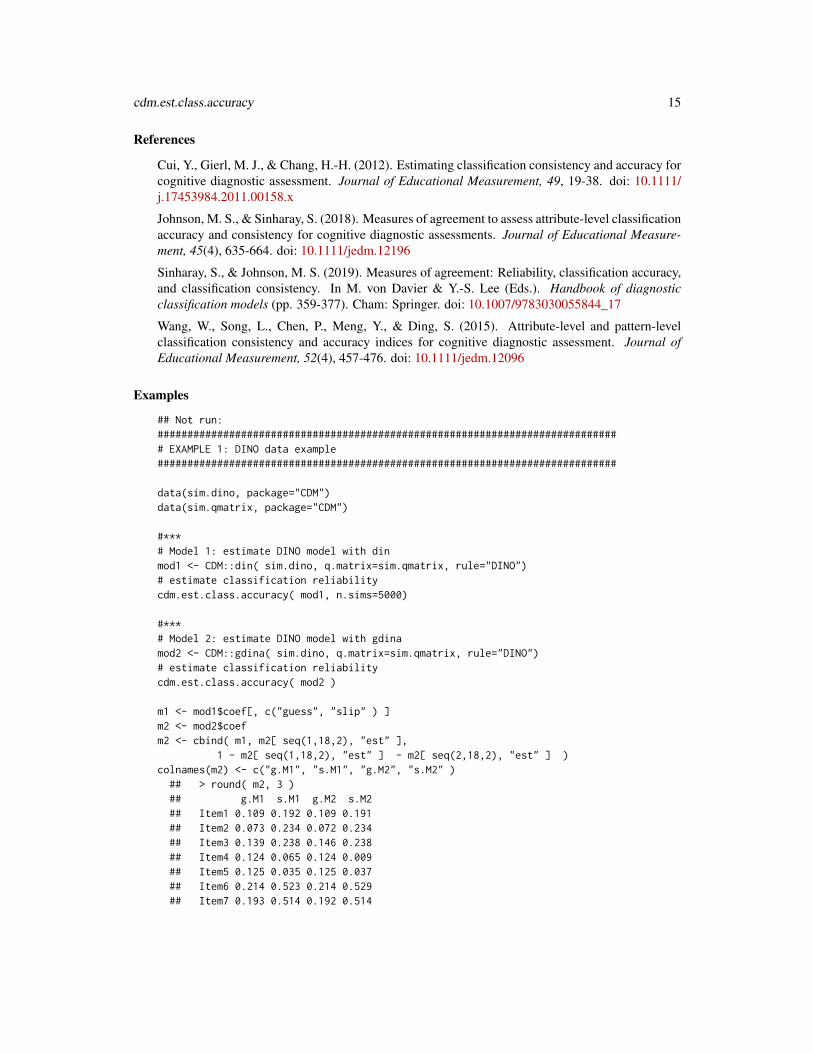
m1 <- mod1$coef[, c("guess", "slip" ) ]m2 <- mod2$coefm2 <- cbind( m1, m2[ seq(1,18,2), "est" ],

1 - m2[ seq(1,18,2), "est" ] - m2[ seq(2,18,2), "est" ] )colnames(m2) <- c("g.M1", "s.M1", "g.M2", "s.M2" )

## > round( m2, 3 )## g.M1 s.M1 g.M2 s.M2## Item1 0.109 0.192 0.109 0.191## Item2 0.073 0.234 0.072 0.234## Item3 0.139 0.238 0.146 0.238## Item4 0.124 0.065 0.124 0.009## Item5 0.125 0.035 0.125 0.037## Item6 0.214 0.523 0.214 0.529## Item7 0.193 0.514 0.192 0.514

https://doi.org/10.1111/j.1745-3984.2011.00158.x

https://doi.org/10.1111/j.1745-3984.2011.00158.x

https://doi.org/10.1111/jedm.12196

https://doi.org/10.1007/978-3-030-05584-4_17

https://doi.org/10.1111/jedm.12096

16 coef

## Item8 0.246 0.100 0.246 0.100## Item9 0.201 0.032 0.195 0.032

# Note that s (the slipping parameter) substantially differs for Item4# for DINO estimation in 'din' and 'gdina'

## End(Not run)

coef Extract Estimated Item Parameters and Skill Class Distribution Pa-rameters

Description

Extracts the estimated parameters from either din, gdina, gdina or gdm objects.

Usage

## S3 method for class 'din'coef(object, ...)

## S3 method for class 'gdina'coef(object, ...)

## S3 method for class 'mcdina'coef(object, ...)

## S3 method for class 'gdm'coef(object, ...)

## S3 method for class 'slca'coef(object, ...)

Arguments

object An object inheriting from either class din, class gdina, class mcdina, class slcaor class gdm.

... Additional arguments to be passed.

Value

A vector, a matrix or a data frame of the estimated parameters for the fitted model.

See Also

din, gdina, gdm, mcdina, slca

Data-sim 17

Examples


# DINA modeld1 <- CDM::din( sim.dina, q.matrix=sim.qmatrix)coef(d1)

## Not run:# GDINA modeld2 <- CDM::gdina( sim.dina, q.matrix=sim.qmatrix)coef(d2)

# GDM modeltheta.k <- seq(-4,4,len=11)d3 <- CDM::gdm( sim.dina, irtmodel="2PL", theta.k=theta.k,

Qmatrix=as.matrix(sim.qmatrix), centered.latent=TRUE)coef(d3)

## End(Not run)

Data-sim Artificial Data: DINA and DINO

Description

Artificial data: dichotomously coded fictitious answers of 400 respondents to 9 items assuming 3underlying attributes.

Usage

data(sim.dina)data(sim.dino)data(sim.qmatrix)

Format

The sim.dina and sim.dino data sets include dichotomous answers of N = 400 respondents toJ = 9 items, thus they are 400× 9 data matrices. For both data sets K = 3 attributes are assumedto underlie the process of responding, stored in sim.qmatrix.

The sim.dina data set is simulated according to the DINA condensation rule, whereas the sim.dinodata set is simulated according to the DINO condensation rule. The slipping errors for the items 1to 9 in both data sets are 0.20,0.20,0.20,0.20,0.00,0.50,0.50,0.10,0.03 and the guessingerrors are 0.10,0.125,0.15,0.175,0.2,0.225,0.25,0.275,0.3. The attributes are assumed tobe mastered with expected probabilities of -0.4,0.2,0.6, respectively. The correlation of the at-tributes is 0.3 for attributes 1 and 2, 0.4 for attributes 1 and 3 and 0.1 for attributes 2 and 3.

18 data.cdm

Example Index

Dataset sim.dina

anova (Examples 1, 2), cdi.kli (Example 1), din (Examples 2, 4, 5), gdina (Example 1), itemfit.sx2(Example 2), modelfit.cor.din (Example 1)

Dataset sim.dino

cdm.est.class.accuracy (Example 1), din (Example 3), gdina (Examples 2, 3, 4),

References

Rupp, A. A., Templin, J. L., & Henson, R. A. (2010) Diagnostic Measurement: Theory, Methods,and Applications. New York: The Guilford Press.

data.cdm Several Datasets for the CDM Package

Description

Several datasets for the CDM package

Usage

data(data.cdm01)data(data.cdm02)data(data.cdm03)data(data.cdm04)data(data.cdm05)data(data.cdm06)data(data.cdm07)data(data.cdm08)data(data.cdm09)data(data.cdm10)

Format

• Dataset data.cdm01This dataset is a multiple choice dataset and used in the mcdina function. The format is:List of 3$ data :'data.frame':..$ I1 : int [1:5003] 3 3 4 1 1 1 1 1 1 1 .....$ I2 : int [1:5003] 1 1 3 1 1 2 1 1 2 1 .....$ I3 : int [1:5003] 4 3 2 3 2 2 2 2 1 2 .....$ I4 : int [1:5003] 3 3 3 2 2 2 2 3 3 1 .....$ I5 : int [1:5003] 2 2 2 3 1 1 2 3 2 1 .....$ I6 : int [1:5003] 3 1 1 1 1 2 1 1 1 1 ...

data.cdm 19

..$ I7 : int [1:5003] 1 1 2 2 1 3 1 1 1 3 ...

..$ I8 : int [1:5003] 1 1 1 1 1 2 1 4 3 3 ...

..$ I9 : int [1:5003] 3 2 1 1 1 1 3 3 1 3 ...

..$ I10: int [1:5003] 2 1 2 1 1 2 2 2 2 1 ...

..$ I11: int [1:5003] 2 2 2 2 1 2 1 2 1 1 ...

..$ I12: int [1:5003] 1 2 1 1 2 1 1 1 1 2 ...

..$ I13: int [1:5003] 2 1 1 1 2 1 2 2 1 1 ...

..$ I14: int [1:5003] 1 1 1 1 1 2 1 1 2 1 ...

..$ I15: int [1:5003] 1 2 1 1 1 1 1 1 1 1 ...

..$ I16: int [1:5003] 1 2 2 1 2 2 2 1 1 1 ...

..$ I17: int [1:5003] 1 1 1 1 1 1 1 1 1 1 ...$ group : int [1:5003] 1 1 1 1 1 1 1 1 1 1 ...$ q.matrix:'data.frame':..$ item : int [1:52] 1 1 1 1 2 2 2 2 3 3 .....$ categ: int [1:52] 1 2 3 4 1 2 3 4 1 2 .....$ A1 : int [1:52] 0 1 0 1 0 1 1 1 0 0 .....$ A2 : int [1:52] 0 0 1 1 0 0 0 1 0 0 .....$ A3 : int [1:52] 0 0 0 0 0 0 0 0 0 0 ...

• Dataset data.cdm02Multiple choice dataset with a Q-matrix designed for polytomous attributes.List of 2$ data :'data.frame':..$ I1 : int [1:3000] 3 3 4 1 1 1 1 1 1 1 .....$ I2 : int [1:3000] 1 1 3 1 1 2 1 1 2 1 .....$ I3 : int [1:3000] 4 3 2 3 2 2 2 2 1 2 ...[...]..$ B17: num [1:3000] 1 1 1 1 1 1 1 1 1 1 .....$ B18: num [1:3000] 1 1 1 1 2 2 2 2 2 2 ...$ q.matrix:'data.frame':..$ item : int [1:100] 1 1 1 1 2 2 2 2 3 3 .....$ categ: int [1:100] 1 2 3 4 1 2 3 4 1 2 .....$ A1 : num [1:100] 0 1 0 1 0 1 1 1 0 0 .....$ A2 : num [1:100] 0 0 1 1 0 0 0 1 0 0 .....$ A3 : num [1:100] 0 0 0 0 0 0 0 0 0 0 .....$ B1 : num [1:100] 0 0 0 0 0 0 0 0 0 0 ...

• Dataset data.cdm03:This is a resimulated dataset from Chiu, Koehn and Wu (2016) where the data generatingmodel is a reduced RUM model. See Example 1.List of 2$ data : num [1:725,1:16] 0 1 1 1 1 1 1 1 1 1 .....-attr(*,"dimnames")=List of 2.. ..$ : NULL.. ..$ : chr [1:16] "I01" "I02" "I03" "I04" ...$ qmatrix:'data.frame': 16 obs. of 6 variables:..$ item: Factor w/ 16 levels "I01","I02","I03",..: 1 2 3 4 5 6 7 8 9 10 .....$ A1 : int [1:16] 1 0 0 0 0 0 0 0 1 1 ...

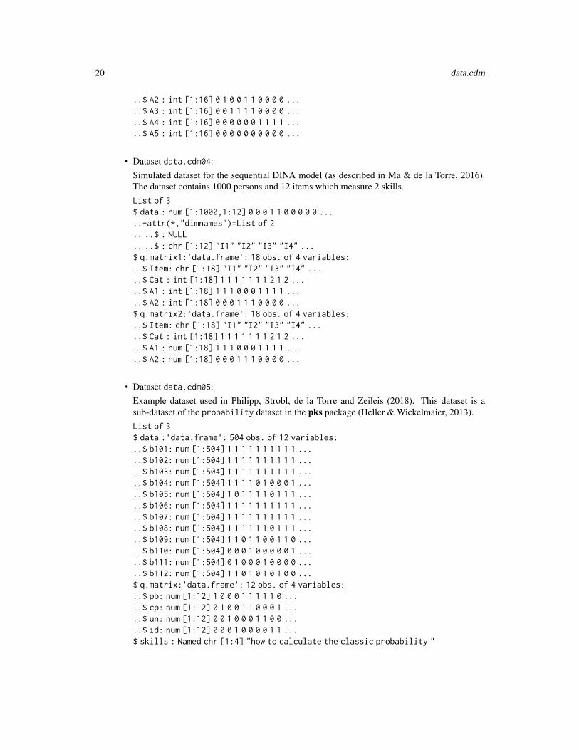
20 data.cdm

..$ A2 : int [1:16] 0 1 0 0 1 1 0 0 0 0 ...

..$ A3 : int [1:16] 0 0 1 1 1 1 0 0 0 0 ...

..$ A4 : int [1:16] 0 0 0 0 0 0 1 1 1 1 ...

..$ A5 : int [1:16] 0 0 0 0 0 0 0 0 0 0 ...

• Dataset data.cdm04:Simulated dataset for the sequential DINA model (as described in Ma & de la Torre, 2016).The dataset contains 1000 persons and 12 items which measure 2 skills.List of 3$ data : num [1:1000,1:12] 0 0 0 1 1 0 0 0 0 0 .....-attr(*,"dimnames")=List of 2.. ..$ : NULL.. ..$ : chr [1:12] "I1" "I2" "I3" "I4" ...$ q.matrix1:'data.frame': 18 obs. of 4 variables:..$ Item: chr [1:18] "I1" "I2" "I3" "I4" .....$ Cat : int [1:18] 1 1 1 1 1 1 1 2 1 2 .....$ A1 : int [1:18] 1 1 1 0 0 0 1 1 1 1 .....$ A2 : int [1:18] 0 0 0 1 1 1 0 0 0 0 ...$ q.matrix2:'data.frame': 18 obs. of 4 variables:..$ Item: chr [1:18] "I1" "I2" "I3" "I4" .....$ Cat : int [1:18] 1 1 1 1 1 1 1 2 1 2 .....$ A1 : num [1:18] 1 1 1 0 0 0 1 1 1 1 .....$ A2 : num [1:18] 0 0 0 1 1 1 0 0 0 0 ...

• Dataset data.cdm05:Example dataset used in Philipp, Strobl, de la Torre and Zeileis (2018). This dataset is asub-dataset of the probability dataset in the pks package (Heller & Wickelmaier, 2013).List of 3$ data :'data.frame': 504 obs. of 12 variables:..$ b101: num [1:504] 1 1 1 1 1 1 1 1 1 1 .....$ b102: num [1:504] 1 1 1 1 1 1 1 1 1 1 .....$ b103: num [1:504] 1 1 1 1 1 1 1 1 1 1 .....$ b104: num [1:504] 1 1 1 1 0 1 0 0 0 1 .....$ b105: num [1:504] 1 0 1 1 1 1 0 1 1 1 .....$ b106: num [1:504] 1 1 1 1 1 1 1 1 1 1 .....$ b107: num [1:504] 1 1 1 1 1 1 1 1 1 1 .....$ b108: num [1:504] 1 1 1 1 1 1 0 1 1 1 .....$ b109: num [1:504] 1 1 0 1 1 0 0 1 1 0 .....$ b110: num [1:504] 0 0 0 1 0 0 0 0 0 1 .....$ b111: num [1:504] 0 1 0 0 0 1 0 0 0 0 .....$ b112: num [1:504] 1 1 0 1 0 1 0 1 0 0 ...$ q.matrix:'data.frame': 12 obs. of 4 variables:..$ pb: num [1:12] 1 0 0 0 1 1 1 1 1 0 .....$ cp: num [1:12] 0 1 0 0 1 1 0 0 0 1 .....$ un: num [1:12] 0 0 1 0 0 0 1 1 0 0 .....$ id: num [1:12] 0 0 0 1 0 0 0 0 1 1 ...$ skills : Named chr [1:4] "how to calculate the classic probability "

data.cdm 21

..-attr(*,"names")=chr [1:4] "pb" "cp" "un" "id"

• Dataset data.cdm06:Resimulated example dataset from Chen and Chen (2017).List of 3$ data :'data.frame': 2733 obs. of 15 variables:..$ I01: num [1:2733] 1 0 0 1 0 0 0 1 1 1 .....$ I02: num [1:2733] 1 0 0 1 1 0 1 0 0 1 .....$ I03: num [1:2733] 0 0 0 1 1 0 1 0 1 0 .....$ I04: num [1:2733] 1 1 0 0 0 0 1 1 1 0 .....$ I05: num [1:2733] 1 0 1 1 0 1 1 1 1 1 .....$ I06: num [1:2733] 0 0 0 1 1 0 0 0 1 1 .....$ I07: num [1:2733] 1 1 1 0 0 1 1 0 1 1 .....$ I08: num [1:2733] 0 0 0 0 0 0 0 0 1 1 .....$ I09: num [1:2733] 1 0 0 1 1 1 0 1 0 1 .....$ I10: num [1:2733] 0 0 0 1 0 1 1 0 1 1 .....$ I11: num [1:2733] 0 1 0 1 1 1 1 0 1 1 .....$ I12: num [1:2733] 0 1 0 1 0 0 0 1 1 1 .....$ I13: num [1:2733] 0 0 1 1 0 1 0 0 0 1 .....$ I14: num [1:2733] 0 0 0 1 1 0 1 1 0 0 .....$ I15: num [1:2733] 0 0 0 1 0 0 1 0 1 1 ...$ q.matrix:'data.frame': 15 obs. of 5 variables:..$ RI: num [1:15] 1 1 1 0 1 1 1 1 0 0 .....$ JS: num [1:15] 1 0 0 1 0 0 0 0 0 1 .....$ GI: num [1:15] 0 1 0 1 0 0 1 1 1 1 .....$ II: num [1:15] 0 1 1 0 1 0 1 0 0 0 .....$ MI: num [1:15] 0 0 1 0 0 0 0 0 1 0 ...$ skills : chr [1:5,1:2] "Retrieving explicit information " .....-attr(*,"dimnames")=List of 2.. ..$ : chr [1:5] "RI" "JS" "GI" "II" ..... ..$ : chr [1:2] "skill" "description"

• Dataset data.cdm07:This is a resimulated dataset from the social anxiety disorder data concerning social phobiawhich involve 13 dichotomous questions (Fang, Liu & Ling, 2017). The simulation was basedon a latent class model with five classes. The dataset was also used in Chen, Li, Liu and Ying(2017).$ data : num [1:863,1:13] 1 0 1 1 1 1 1 1 1 1 .....-attr(*,"dimnames")=List of 2.. ..$ : NULL.. ..$ : chr [1:13] "I1" "I2" "I3" "I4" ...$ q.matrix: num [1:13,1:3] 1 1 1 1 0 0 0 0 0 0 .....-attr(*,"dimnames")=List of 2.. ..$ : chr [1:13] "I1" "I2" "I3" "I4" ..... ..$ : chr [1:3] "A1" "A2" "A3"$ items : atomic [1:13] 1 speaking in front of other people? .....-attr(*,"stem")=chr "Have you ever had a strong fear or avoidance of ..."

22 data.cdm

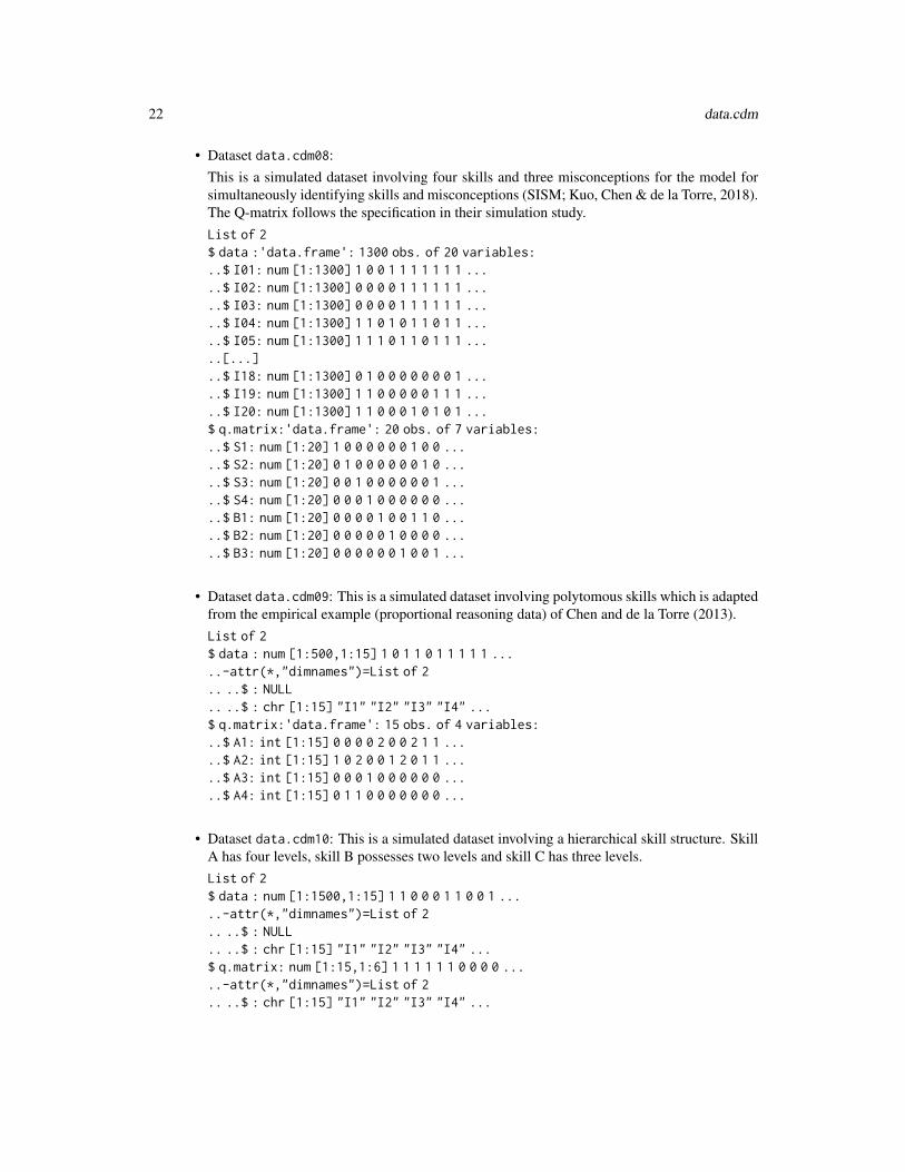
• Dataset data.cdm08:This is a simulated dataset involving four skills and three misconceptions for the model forsimultaneously identifying skills and misconceptions (SISM; Kuo, Chen & de la Torre, 2018).The Q-matrix follows the specification in their simulation study.List of 2$ data :'data.frame': 1300 obs. of 20 variables:..$ I01: num [1:1300] 1 0 0 1 1 1 1 1 1 1 .....$ I02: num [1:1300] 0 0 0 0 1 1 1 1 1 1 .....$ I03: num [1:1300] 0 0 0 0 1 1 1 1 1 1 .....$ I04: num [1:1300] 1 1 0 1 0 1 1 0 1 1 .....$ I05: num [1:1300] 1 1 1 0 1 1 0 1 1 1 .....[...]..$ I18: num [1:1300] 0 1 0 0 0 0 0 0 0 1 .....$ I19: num [1:1300] 1 1 0 0 0 0 0 1 1 1 .....$ I20: num [1:1300] 1 1 0 0 0 1 0 1 0 1 ...$ q.matrix:'data.frame': 20 obs. of 7 variables:..$ S1: num [1:20] 1 0 0 0 0 0 0 1 0 0 .....$ S2: num [1:20] 0 1 0 0 0 0 0 0 1 0 .....$ S3: num [1:20] 0 0 1 0 0 0 0 0 0 1 .....$ S4: num [1:20] 0 0 0 1 0 0 0 0 0 0 .....$ B1: num [1:20] 0 0 0 0 1 0 0 1 1 0 .....$ B2: num [1:20] 0 0 0 0 0 1 0 0 0 0 .....$ B3: num [1:20] 0 0 0 0 0 0 1 0 0 1 ...

• Dataset data.cdm09: This is a simulated dataset involving polytomous skills which is adaptedfrom the empirical example (proportional reasoning data) of Chen and de la Torre (2013).List of 2$ data : num [1:500,1:15] 1 0 1 1 0 1 1 1 1 1 .....-attr(*,"dimnames")=List of 2.. ..$ : NULL.. ..$ : chr [1:15] "I1" "I2" "I3" "I4" ...$ q.matrix:'data.frame': 15 obs. of 4 variables:..$ A1: int [1:15] 0 0 0 0 2 0 0 2 1 1 .....$ A2: int [1:15] 1 0 2 0 0 1 2 0 1 1 .....$ A3: int [1:15] 0 0 0 1 0 0 0 0 0 0 .....$ A4: int [1:15] 0 1 1 0 0 0 0 0 0 0 ...

• Dataset data.cdm10: This is a simulated dataset involving a hierarchical skill structure. SkillA has four levels, skill B possesses two levels and skill C has three levels.List of 2$ data : num [1:1500,1:15] 1 1 0 0 0 1 1 0 0 1 .....-attr(*,"dimnames")=List of 2.. ..$ : NULL.. ..$ : chr [1:15] "I1" "I2" "I3" "I4" ...$ q.matrix: num [1:15,1:6] 1 1 1 1 1 1 0 0 0 0 .....-attr(*,"dimnames")=List of 2.. ..$ : chr [1:15] "I1" "I2" "I3" "I4" ...

data.cdm 23

.. ..$ : chr [1:6] "A1" "A2" "A3" "B1" ...

References

Chen, H., & Chen, J. (2017). Cognitive diagnostic research on chinese students’ English lis-tening skills and implications on skill training. English Language Teaching, 10(12), 107-115.http://dx.doi.org/10.5539/elt.v10n12p107

Chen, J., & de la Torre, J. (2013). A general cognitive diagnosis model for expert-defined polyto-mous attributes. Applied Psychological Measurement, 37, 419-437. http://dx.doi.org/10.1177/0146621613479818

Chen, Y., Li, X., Liu, J., & Ying, Z. (2017). Regularized latent class analysis with application incognitive diagnosis. Psychometrika, 82, 660-692. http://dx.doi.org/10.1007/s11336-016-9545-6

Chiu, C.-Y., Koehn, H.-F., & Wu, H.-M. (2016). Fitting the reduced RUM with Mplus: A tutorial.International Journal of Testing, 16(4), 331-351. http://dx.doi.org/10.1080/15305058.2016.1148038

Fang, G., Liu, J., & Ying, Z. (2017). On the identifiability of diagnostic classification models.arXiv, 1706.01240. https://arxiv.org/abs/1706.01240

Heller, J. and Wickelmaier, F. (2013). Minimum discrepancy estimation in probabilistic knowledgestructures. Electronic Notes in Discrete Mathematics, 42, 49-56.http://dx.doi.org/10.1016/j.endm.2013.05.145

Kuo, B.-C., Chen, C.-H., & de la Torre, J. (2018). A cognitive diagnosis model for identify-ing coexisting skills and misconceptions. Applied Psychological Measurement, 42(3), 179-191.http://dx.doi.org/10.1177/0146621617722791

Ma, W., & de la Torre, J. (2016). A sequential cognitive diagnosis model for polytomous responses.British Journal of Mathematical and Statistical Psychology, 69(3), 253-275.https://doi.org/10.1111/bmsp.12070

Philipp, M., Strobl, C., de la Torre, J., & Zeileis, A. (2018). On the estimation of standard errorsin cognitive diagnosis models. Journal of Educational and Behavioral Statistics, 43(1), 88-115.http://dx.doi.org/10.3102/1076998617719728

Examples

## Not run:############################################################################## EXAMPLE 1: Reduced RUM model, Chiu et al. (2016)#############################################################################

data(data.cdm03, package="CDM")dat <- data.cdm03$dataqmatrix <- data.cdm03$qmatrix

#*** Model 1: Reduced RUMmod1 <- CDM::gdina( dat, q.matrix=qmatrix[,-1], rule="RRUM" )summary(mod1)

#*** Model 2: Additive model with identity link functionmod2 <- CDM::gdina( dat, q.matrix=qmatrix[,-1], rule="ACDM" )summary(mod2)

24 data.dcm

#*** Model 3: Additive model with logit link functionmod3 <- CDM::gdina( dat, q.matrix=qmatrix[,-1], rule="ACDM", linkfct="logit")summary(mod3)

############################################################################## EXAMPLE 2: GDINA model - probability dataset from the pks package#############################################################################

data(data.cdm05, package="CDM")dat <- data.cdm05$dataQ <- data.cdm05$q.matrix

#* estimate modelmod1 <- CDM::gdina( dat, q.matrix=Q )summary(mod1)

## End(Not run)

data.dcm Dataset from Book ’Diagnostic Measurement’ of Rupp, Templin andHenson (2010)

Description

Dataset from Chapter 9 of the book ’Diagnostic Measurement’ (Rupp, Templin & Henson, 2010).

Usage

data(data.dcm)

Format

The format of the data is a list containing the dichotomous item response data data (10000 personsat 7 items) and the Q-matrix q.matrix (7 items and 3 skills):

List of 2$ data :'data.frame':..$ id: int [1:10000] 1 2 3 4 5 6 7 8 9 10 .....$ D1: num [1:10000] 0 0 0 0 1 0 1 0 0 1 .....$ D2: num [1:10000] 0 0 0 0 0 1 1 1 0 1 .....$ D3: num [1:10000] 1 0 1 0 1 1 0 0 0 1 .....$ D4: num [1:10000] 0 0 1 0 0 1 1 1 0 0 .....$ D5: num [1:10000] 1 0 0 0 1 1 1 0 1 0 .....$ D6: num [1:10000] 0 0 0 0 1 1 1 0 0 1 .....$ D7: num [1:10000] 0 0 0 0 0 1 1 0 1 1 ...$ q.matrix: num [1:7,1:3] 1 0 0 1 1 0 1 0 1 0 .....-attr(*,"dimnames")=List of 2.. ..$ : chr [1:7] "D1" "D2" "D3" "D4" ..... ..$ : chr [1:3] "skill1" "skill2" "skill3"

data.dcm 25

Source

For supplementary material of the Rupp, Templin and Henson book (2010) see http://dcm.coe.uga.edu/.

The dataset was downloaded from http://dcm.coe.uga.edu/supplemental/chapter9.html.

References


Examples

## Not run:data(data.dcm, package="CDM")

dat <- data.dcm$data[,-1]Q <- data.dcm$q.matrix

#*****************************************************# Model 1: DINA model#*****************************************************mod1 <- CDM::din( dat, q.matrix=Q )summary(mod1)

#--------# Model 1m: estimate model in mirt packagelibrary(mirt)library(sirt)

#** define theta grid of skills# use the function skillspace.hierarchy just for convenience

hier <- "skill1 > skill2"skillspace <- CDM::skillspace.hierarchy( hier, skill.names=colnames(Q) )Theta <- as.matrix(skillspace$skillspace.complete)

#** create mirt modelmirtmodel <- mirt::mirt.model("

skill1=1skill2=2skill3=3(skill1*skill2)=4(skill1*skill3)=5(skill2*skill3)=6(skill1*skill2*skill3)=7

" )#** mirt parameter table

mod.pars <- mirt::mirt( dat, mirtmodel, pars="values")# use starting values of .20 for guessing parameter

ind <- which( mod.pars$name=="d" )mod.pars[ind,"value"] <- stats::qlogis(.20) # guessing parameter on the logit metric

# use starting values of .80 for anti-slipping parameterind <- which( ( mod.pars$name %in% paste0("a",1:20 ) ) & (mod.pars$est) )

http://dcm.coe.uga.edu/

http://dcm.coe.uga.edu/

http://dcm.coe.uga.edu/supplemental/chapter9.html

26 data.dcm

mod.pars[ind,"value"] <- stats::qlogis(.80) - stats::qlogis(.20)mod.pars

#** prior for the skill space distributionI <- ncol(dat)lca_prior <- function(Theta,Etable){

TP <- nrow(Theta)if ( is.null(Etable) ){ prior <- rep( 1/TP, TP ) }if ( ! is.null(Etable) ){prior <- ( rowSums(Etable[, seq(1,2*I,2)]) + rowSums(Etable[,seq(2,2*I,2)]) )/I

}prior <- prior / sum(prior)return(prior)}

#** estimate model in mirtmod1m <- mirt::mirt(dat, mirtmodel, pars=mod.pars, verbose=TRUE,

technical=list( customTheta=Theta, customPriorFun=lca_prior) )# The number of estimated parameters is incorrect because mirt does not correctly count# estimated parameters from the user customized prior distribution.

mod1m@nest <- as.integer(sum(mod.pars$est) + nrow(Theta) - 1)# extract log-likelihood

mod1m@logLik# compute AIC and BIC

( AIC <- -2*mod1m@logLik+2*mod1m@nest )( BIC <- -2*mod1m@logLik+log(mod1m@Data$N)*mod1m@nest )

#** extract item parameterscmod1m <- sirt::mirt.wrapper.coef(mod1m)$coef# compare estimated guessing and slipping parametersdfr <- data.frame( "din.guess"=mod1$guess$est,

"mirt.guess"=plogis(cmod1m$d), "din.slip"=mod1$slip$est,"mirt.slip"=1-plogis( rowSums( cmod1m[, c("d", paste0("a",1:7) ) ] ) )

)round(t(dfr),3)

## [,1] [,2] [,3] [,4] [,5] [,6] [,7]## din.guess 0.217 0.193 0.189 0.135 0.143 0.135 0.162## mirt.guess 0.226 0.189 0.184 0.132 0.142 0.132 0.158## din.slip 0.338 0.331 0.334 0.220 0.222 0.211 0.042## mirt.slip 0.339 0.333 0.336 0.223 0.225 0.214 0.044

# compare estimated skill class distributiondfr <- data.frame("din"=mod1$attribute.patt$class.prob,

"mirt"=mod1m@Prior[[1]] )round(t(dfr),3)

## [,1] [,2] [,3] [,4] [,5] [,6] [,7] [,8]## din 0.113 0.083 0.094 0.092 0.064 0.059 0.065 0.429## mirt 0.116 0.074 0.095 0.064 0.095 0.058 0.066 0.433

#** extract estimated classificationsfsc1m <- sirt::mirt.wrapper.fscores( mod1m )#- estimated reliabilitiesfsc1m$EAP.rel

## skill1 skill2 skill3## 0.5479942 0.5362595 0.5357961

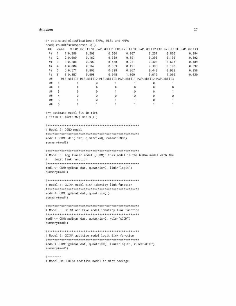
data.dcm 27

#- estimated classfications: EAPs, MLEs and MAPshead( round(fsc1m$person,3) )## case M EAP.skill1 SE.EAP.skill1 EAP.skill2 SE.EAP.skill2 EAP.skill3 SE.EAP.skill3## 1 1 0.286 0.508 0.500 0.067 0.251 0.820 0.384## 2 2 0.000 0.162 0.369 0.191 0.393 0.190 0.392## 3 3 0.286 0.200 0.400 0.211 0.408 0.607 0.489## 4 4 0.000 0.162 0.369 0.191 0.393 0.190 0.392## 5 5 0.571 0.802 0.398 0.267 0.443 0.928 0.258## 6 6 0.857 0.998 0.045 1.000 0.019 1.000 0.020## MLE.skill1 MLE.skill2 MLE.skill3 MAP.skill1 MAP.skill2 MAP.skill3## 1 1 0 1 1 0 1## 2 0 0 0 0 0 0## 3 0 0 1 0 0 1## 4 0 0 0 0 0 0## 5 1 0 1 1 0 1## 6 1 1 1 1 1 1

#** estimate model fit in mirt( fit1m <- mirt::M2( mod1m ) )

#*****************************************************# Model 2: DINO model#*****************************************************mod2 <- CDM::din( dat, q.matrix=Q, rule="DINO")summary(mod2)

#*****************************************************# Model 3: log-linear model (LCDM): this model is the GDINA model with the# logit link function#*****************************************************mod3 <- CDM::gdina( dat, q.matrix=Q, link="logit")summary(mod3)

#*****************************************************# Model 4: GDINA model with identity link function#*****************************************************mod4 <- CDM::gdina( dat, q.matrix=Q )summary(mod4)

#*****************************************************# Model 5: GDINA additive model identity link function#*****************************************************mod5 <- CDM::gdina( dat, q.matrix=Q, rule="ACDM")summary(mod5)

#*****************************************************# Model 6: GDINA additive model logit link function#*****************************************************mod6 <- CDM::gdina( dat, q.matrix=Q, link="logit", rule="ACDM")summary(mod6)

#--------# Model 6m: GDINA additive model in mirt package

28 data.dcm

# use data specifications from Model 1m)#** create mirt model

mirtmodel <- mirt::mirt.model("skill1=1,4,5,7skill2=2,4,6,7skill3=3,5,6,7

" )#** mirt parameter table

mod.pars <- mirt::mirt( dat, mirtmodel, pars="values")#** estimate model in mirt# Theta and lca_prior as defined as in Model 1m

mod6m <- mirt::mirt(dat, mirtmodel, pars=mod.pars, verbose=TRUE,technical=list( customTheta=Theta, customPriorFun=lca_prior) )

mod6m@nest <- as.integer(sum(mod.pars$est) + nrow(Theta) - 1)# extract log-likelihood

mod6m@logLik# compute AIC and BIC

( AIC <- -2*mod6m@logLik+2*mod6m@nest )( BIC <- -2*mod6m@logLik+log(mod6m@Data$N)*mod6m@nest )

#** skill distributionmod6m@Prior[[1]]#** extract item parameters

cmod6m <- mirt.wrapper.coef(mod6m)$coefprint(cmod6m,digits=4)

## item a1 a2 a3 d g u## 1 D1 1.882 0.000 0.000 -0.9330 0 1## 2 D2 0.000 2.049 0.000 -1.0430 0 1## 3 D3 0.000 0.000 2.028 -0.9915 0 1## 4 D4 2.697 2.525 0.000 -2.9925 0 1## 5 D5 2.524 0.000 2.478 -2.7863 0 1## 6 D6 0.000 2.818 2.791 -3.1324 0 1## 7 D7 3.113 2.918 2.785 -4.2794 0 1

#*****************************************************# Model 7: Reduced RUM model#*****************************************************mod7 <- CDM::gdina( dat, q.matrix=Q, rule="RRUM")summary(mod7)

#*****************************************************# Model 8: latent class model with 3 classes and 4 sets of starting values#*****************************************************

#-- Model 8a: randomLCA packagelibrary(randomLCA)mod8a <- randomLCA::randomLCA( dat, nclass=3, verbose=TRUE, notrials=4)

#-- Model8b: rasch.mirtlc function in sirt packagelibrary(sirt)mod8b <- sirt::rasch.mirtlc( dat, Nclasses=3, nstarts=4 )summary(mod8a)summary(mod8b)

data.dtmr 29

## End(Not run)

data.dtmr DTMR Fraction Data (Bradshaw et al., 2014)

Description

This is a simulated dataset of the DTMR fraction data described in Bradshaw, Izsak, Templin andJacobson (2014).

Usage

data(data.dtmr)

Format

The format is:

List of 5$ data : num [1:5000,1:27] 0 0 0 0 0 1 0 0 1 1 .....-attr(*,"dimnames")=List of 2.. ..$ : NULL.. ..$ : chr [1:27] "M1" "M2" "M3" "M4" ...$ q.matrix :'data.frame': 27 obs. of 4 variables:..$ RU : int [1:27] 1 0 0 1 1 0 1 0 0 0 .....$ PI : int [1:27] 0 0 1 0 0 1 0 0 0 0 .....$ APP: int [1:27] 0 1 0 0 0 0 0 1 1 1 .....$ MC : int [1:27] 0 0 0 0 0 0 0 0 0 0 ...$ skill.distribution:'data.frame': 16 obs. of 5 variables:..$ RU : int [1:16] 0 0 0 0 0 0 0 0 1 1 .....$ PI : int [1:16] 0 0 0 0 1 1 1 1 0 0 .....$ APP : int [1:16] 0 0 1 1 0 0 1 1 0 0 .....$ MC : int [1:16] 0 1 0 1 0 1 0 1 0 1 .....$ freq: int [1:16] 1064 350 280 406 196 126 238 770 14 28 ...$ itempars :'data.frame': 27 obs. of 7 variables:..$ item : chr [1:27] "M1" "M2" "M3" "M4" .....$ lam0 : num [1:27] -1.12 0.59 -2.07 -1.19 -1.67 -3.81 -0.73 -0.62 -0.09 0.28 .....$ RU : num [1:27] 2.24 0 0 0.65 1.52 0 1.2 0 0 0 .....$ PI : num [1:27] 0 0 1.7 0 0 2.08 0 0 0 0 .....$ APP : num [1:27] 0 1.27 0 0 0 0 0 4.25 2.16 0.87 .....$ MC : num [1:27] 0 0 0 0 0 0 0 0 0 0 .....$ RU.PI: num [1:27] 0 0 0 0 0 0 0 0 0 0 ...$ sim_data :function (N,skill.distribution,itempars)..-attr(*,"srcref")='srcref' int [1:8] 1 13 20 1 13 1 1 20.. ..-attr(*,"srcfile")=Classes 'srcfilecopy','srcfile' <environment: 0x00000000298a8ed0>

The attribute definition are as follows

30 data.dtmr

RU: Referent units

PI: Partitioning and iterating attribute

APP: Appropriateness attribute

MC: Multiplicative Comparison attribute

Source

Simulated dataset according to Bradshaw et al. (2014).

References

Bradshaw, L., Izsak, A., Templin, J., & Jacobson, E. (2014). Diagnosing teachers’ understandingsof rational numbers: Building a multidimensional test within the diagnostic classification frame-work. Educational Measurement: Issues and Practice, 33, 2-14.

Examples

## Not run:############################################################################## EXAMPLE 1: Model comparisons data.dtmr#############################################################################

data(data.dtmr, package="CDM")data <- data.dtmr$dataq.matrix <- data.dtmr$q.matrixI <- ncol(data)

#*** Model 1: LCDM# define item wise rulesrule <- rep( "ACDM", I )names(rule) <- colnames(data)rule[ c("M14","M17") ] <- "GDINA2"# estimate modelmod1 <- CDM::gdina( data, q.matrix, linkfct="logit", rule=rule)summary(mod1)

#*** Model 2: DINA modelmod2 <- CDM::gdina( data, q.matrix, rule="DINA" )summary(mod2)

#*** Model 3: RRUM modelmod3 <- CDM::gdina( data, q.matrix, rule="RRUM" )summary(mod3)

#--- model comparisons

# LCDM vs. DINAanova(mod1,mod2)

## Model loglike Deviance Npars AIC BIC Chisq df p## 2 Model 2 -76570.89 153141.8 69 153279.8 153729.5 1726.645 10 0## 1 Model 1 -75707.57 151415.1 79 151573.1 152088.0 NA NA NA

data.ecpe 31

# LCDM vs. RRUManova(mod1,mod3)


#--- model fitsummary( CDM::modelfit.cor.din( mod1 ) )

## Test of Global Model Fit## type value p## 1 max(X2) 7.74382 1.00000## 2 abs(fcor) 0.04056 0.72707#### Fit Statistics## est## MADcor 0.00959## SRMSR 0.01217## MX2 0.75696## 100*MADRESIDCOV 0.20283## MADQ3 0.02220

############################################################################## EXAMPLE 2: Simulating data of structure data.dtmr#############################################################################

data(data.dtmr, package="CDM")

# draw sample of N=200set.seed(87)data.dtmr$sim_data(N=200, skill.distribution=data.dtmr$skill.distribution,

itempars=data.dtmr$itempars)

## End(Not run)

data.ecpe Dataset ECPE

Description

ECPE dataset from the Templin and Hoffman (2013) tutorial of specifying cognitive diagnosticmodels in Mplus.

Usage

data(data.ecpe)

32 data.ecpe

Format

The format of the data is a list containing the dichotomous item response data data (2922 personsat 28 items) and the Q-matrix q.matrix (28 items and 3 skills):

List of 2$ data :'data.frame':..$ id : int [1:2922] 1 2 3 4 5 6 7 8 9 10 .....$ E1 : int [1:2922] 1 1 1 1 1 1 1 0 1 1 .....$ E2 : int [1:2922] 1 1 1 1 1 1 1 1 1 1 .....$ E3 : int [1:2922] 1 1 1 1 1 1 1 1 1 1 .....$ E4 : int [1:2922] 0 1 1 1 1 1 1 1 1 1 ...[...]..$ E27: int [1:2922] 1 1 1 1 1 1 1 0 1 1 .....$ E28: int [1:2922] 1 1 1 1 1 1 1 1 1 1 ...$ q.matrix:'data.frame':..$ skill1: int [1:28] 1 0 1 0 0 0 1 0 0 1 .....$ skill2: int [1:28] 1 1 0 0 0 0 0 1 0 0 .....$ skill3: int [1:28] 0 0 1 1 1 1 1 0 1 0 ...

The skills are

skill1: Morphosyntactic rules

skill2: Cohesive rules

skill3: Lexical rules.

Details

The dataset has been used in Templin and Hoffman (2013), and Templin and Bradshaw (2014).

Source

The dataset was downloaded from http://psych.unl.edu/jtemplin/teaching/dcm/dcm12ncme/.

References

Templin, J., & Bradshaw, L. (2014). Hierarchical diagnostic classification models: A family ofmodels for estimating and testing attribute hierarchies. Psychometrika, 79, 317-339.

Templin, J., & Hoffman, L. (2013). Obtaining diagnostic classification model estimates usingMplus. Educational Measurement: Issues and Practice, 32, 37-50.

See Also

GDINA::ecpe

Examples

## Not run:data(data.ecpe, package="CDM")

data.ecpe 33

dat <- data.ecpe$data[,-1]Q <- data.ecpe$q.matrix

#*** Model 1: LCDM modelmod1 <- CDM::gdina( dat, q.matrix=Q, link="logit")summary(mod1)

#*** Model 2: DINA modelmod2 <- CDM::gdina( dat, q.matrix=Q, rule="DINA")summary(mod2)

# Model comparison using likelihood ratio testanova(mod1,mod2)


#*** Model 3: Hierarchical LCDM (HLCDM) | Templin and Bradshaw (2014)# Testing a linear hierarchyhier <- "skill3 > skill2 > skill1"skill.names <- colnames(Q)# define skill space with hierarchyskillspace <- CDM::skillspace.hierarchy( hier, skill.names=skill.names )skillspace$skillspace.reduced

## skill1 skill2 skill3## A000 0 0 0## A001 0 0 1## A011 0 1 1## A111 1 1 1

zeroprob.skillclasses <- skillspace$zeroprob.skillclasses

# define user-defined parameters in LCDM: hierarchical LCDM (HLCDM)Mj.user <- mod1$Mj# select items with require two attributesitems <- which( rowSums(Q) > 1 )# modify design matrix for item parametersfor (ii in items){

m1 <- Mj.user[[ii]]Mj.user[[ii]][[1]] <- (m1[[1]])[,-2]Mj.user[[ii]][[2]] <- (m1[[2]])[-2]

}

# estimate model# note that avoid.zeroprobs is set to TRUE to avoid algorithmic instabilitiesmod3 <- CDM::gdina( dat, q.matrix=Q, link="logit",

zeroprob.skillclasses=zeroprob.skillclasses, Mj=Mj.user,avoid.zeroprobs=TRUE )

summary(mod3)

#*****************************************#** estimate further models

#*** Model 4: RRUM model

34 data.fraction

mod4 <- CDM::gdina( dat, q.matrix=Q, rule="RRUM")summary(mod4)# compare some modelsIRT.compareModels(mod1, mod2, mod3, mod4 )

#*** Model 5a: GDINA model with identity linkmod5a <- CDM::gdina( dat, q.matrix=Q, link="identity")summary(mod5a)#*** Model 5b: GDINA model with logit linkmod5b <- CDM::gdina( dat, q.matrix=Q, link="logit")summary(mod5b)#*** Model 5c: GDINA model with log linkmod5c <- CDM::gdina( dat, q.matrix=Q, link="log")summary(mod5c)# compare modelsIRT.compareModels(mod5a, mod5b, mod5c)

## End(Not run)

data.fraction Fraction Subtraction Dataset with Different Subsets of Data and Dif-ferent Q-Matrices

Description

Contains different sub-datasets of the fraction subtraction data of Tatsuoka with different Q-matrixspecifications.

Usage

data(data.fraction1)data(data.fraction2)data(data.fraction3)data(data.fraction4)data(data.fraction5)

Format

• The dataset data.fraction1 is the fraction subtraction data set with 536 students and 15items. The Q-matrix was defined in de la Torre (2009). This dataset is a list with the dataset(data) and the Q-matrix as entries.The format is:List of 2$ data :'data.frame':..$ T01: int [1:536] 0 1 1 1 0 0 0 0 0 0 .....$ T02: int [1:536] 1 1 1 1 1 0 0 1 0 0 .....$ T03: int [1:536] 0 1 1 1 1 1 0 0 0 0 .....$ T04: int [1:536] 1 1 1 0 0 0 0 0 0 0 ...

data.fraction 35

..$ T05: int [1:536] 0 1 0 0 0 1 1 0 1 1 ...

..$ T06: int [1:536] 1 1 0 1 0 0 0 0 0 0 ...

..$ T07: int [1:536] 1 1 0 1 0 0 0 0 0 0 ...

..$ T08: int [1:536] 1 1 0 1 1 0 0 0 1 1 ...

..$ T09: int [1:536] 1 1 1 1 0 1 0 0 1 0 ...

..$ T10: int [1:536] 1 1 1 0 0 0 0 0 0 0 ...

..$ T11: int [1:536] 1 1 1 1 0 0 0 0 0 0 ...

..$ T12: int [1:536] 0 1 0 0 0 0 0 0 0 0 ...

..$ T13: int [1:536] 1 1 0 1 0 0 0 0 0 0 ...

..$ T14: int [1:536] 1 1 0 0 0 0 0 0 0 0 ...

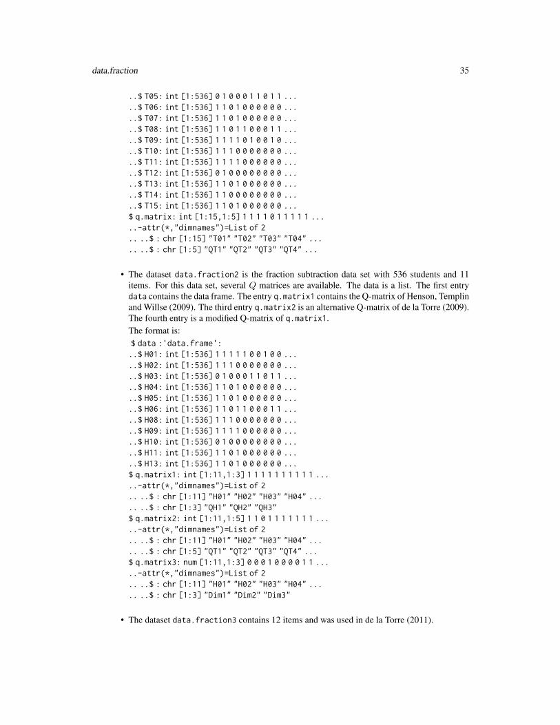
..$ T15: int [1:536] 1 1 0 1 0 0 0 0 0 0 ...$ q.matrix: int [1:15,1:5] 1 1 1 1 0 1 1 1 1 1 .....-attr(*,"dimnames")=List of 2.. ..$ : chr [1:15] "T01" "T02" "T03" "T04" ..... ..$ : chr [1:5] "QT1" "QT2" "QT3" "QT4" ...

• The dataset data.fraction2 is the fraction subtraction data set with 536 students and 11items. For this data set, several Q matrices are available. The data is a list. The first entrydata contains the data frame. The entry q.matrix1 contains the Q-matrix of Henson, Templinand Willse (2009). The third entry q.matrix2 is an alternative Q-matrix of de la Torre (2009).The fourth entry is a modified Q-matrix of q.matrix1.The format is:$ data :'data.frame':..$ H01: int [1:536] 1 1 1 1 1 0 0 1 0 0 .....$ H02: int [1:536] 1 1 1 0 0 0 0 0 0 0 .....$ H03: int [1:536] 0 1 0 0 0 1 1 0 1 1 .....$ H04: int [1:536] 1 1 0 1 0 0 0 0 0 0 .....$ H05: int [1:536] 1 1 0 1 0 0 0 0 0 0 .....$ H06: int [1:536] 1 1 0 1 1 0 0 0 1 1 .....$ H08: int [1:536] 1 1 1 0 0 0 0 0 0 0 .....$ H09: int [1:536] 1 1 1 1 0 0 0 0 0 0 .....$ H10: int [1:536] 0 1 0 0 0 0 0 0 0 0 .....$ H11: int [1:536] 1 1 0 1 0 0 0 0 0 0 .....$ H13: int [1:536] 1 1 0 1 0 0 0 0 0 0 ...$ q.matrix1: int [1:11,1:3] 1 1 1 1 1 1 1 1 1 1 .....-attr(*,"dimnames")=List of 2.. ..$ : chr [1:11] "H01" "H02" "H03" "H04" ..... ..$ : chr [1:3] "QH1" "QH2" "QH3"$ q.matrix2: int [1:11,1:5] 1 1 0 1 1 1 1 1 1 1 .....-attr(*,"dimnames")=List of 2.. ..$ : chr [1:11] "H01" "H02" "H03" "H04" ..... ..$ : chr [1:5] "QT1" "QT2" "QT3" "QT4" ...$ q.matrix3: num [1:11,1:3] 0 0 0 1 0 0 0 0 1 1 .....-attr(*,"dimnames")=List of 2.. ..$ : chr [1:11] "H01" "H02" "H03" "H04" ..... ..$ : chr [1:3] "Dim1" "Dim2" "Dim3"

• The dataset data.fraction3 contains 12 items and was used in de la Torre (2011).

36 data.fraction

List of 2$ data :'data.frame': 536 obs. of 12 variables:..$ B01: int [1:536] 0 1 1 1 0 0 0 0 0 0 .....$ B02: int [1:536] 1 1 1 1 1 0 0 1 0 0 .....$ B03: int [1:536] 0 1 1 1 1 1 0 0 0 0 .....$ B04: int [1:536] 0 1 0 0 0 1 1 0 1 1 .....$ B05: int [1:536] 1 1 0 1 0 0 0 0 0 0 .....$ B06: int [1:536] 1 1 0 1 0 0 0 0 0 0 .....$ B07: int [1:536] 1 1 0 1 1 0 0 0 1 1 .....$ B08: int [1:536] 1 1 1 1 0 1 0 0 1 0 .....$ B09: int [1:536] 1 1 1 1 0 0 0 0 0 0 .....$ B10: int [1:536] 0 1 0 0 0 0 0 0 0 0 .....$ B11: int [1:536] 1 1 0 1 0 0 0 0 0 0 .....$ B12: int [1:536] 1 1 0 1 0 0 0 0 0 0 ...$ q.matrix:'data.frame': 12 obs. of 5 variables:..$ item: Factor w/ 13 levels "","B01","B02",..: 2 3 4 5 6 7 8 9 10 11 .....$ QA1 : int [1:12] 1 1 1 1 1 1 1 1 1 1 .....$ QA2 : int [1:12] 0 1 0 0 1 1 1 0 0 0 .....$ QA3 : int [1:12] 0 1 0 1 1 1 0 1 1 1 .....$ QA4 : int [1:12] 0 1 0 0 1 1 0 0 0 1 ...

• The dataset data.fraction4 contains 17 items and was used in de la Torre and Douglas(2004) and Chen, Liu, Xu and Ying (2015).

List of 2$ data :'data.frame': 536 obs. of 17 variables:..$ A01: int [1:536] 0 0 0 1 0 0 0 0 0 0 .....$ A02: int [1:536] 0 1 1 1 0 0 0 0 0 0 .....$ A03: int [1:536] 0 1 1 1 0 0 0 0 0 0 .....$ A04: int [1:536] 1 1 1 1 1 0 0 1 0 0 .....$ A05: int [1:536] 1 1 0 1 1 0 0 0 1 1 .....$ A06: int [1:536] 1 1 1 1 0 1 0 0 1 0 .....$ A07: int [1:536] 1 1 1 1 0 0 0 0 0 0 .....$ A08: int [1:536] 0 0 0 1 0 0 0 0 0 1 .....$ A09: int [1:536] 1 1 1 0 0 0 0 0 0 0 .....$ A10: int [1:536] 1 1 1 0 0 0 0 0 0 0 .....$ A11: int [1:536] 1 1 0 1 0 0 0 0 0 0 .....$ A12: int [1:536] 1 1 0 1 0 0 0 0 0 0 .....$ A13: int [1:536] 0 1 0 0 0 0 0 0 0 0 .....$ A14: int [1:536] 1 1 0 1 0 0 0 0 0 0 .....$ A15: int [1:536] 1 1 0 0 0 0 0 0 0 0 .....$ A16: int [1:536] 1 1 0 1 0 0 0 0 0 0 .....$ A17: int [1:536] 0 1 0 0 0 0 0 0 0 0 ...$ q.matrix:'data.frame': 17 obs. of 9 variables:..$ item: Factor w/ 18 levels "","A01","A02",..: 2 3 4 5 6 7 8 9 10 11 .....$ QA1 : int [1:17] 0 0 0 0 0 0 0 0 1 0 .....$ QA2 : int [1:17] 0 0 0 1 0 1 1 1 1 1 .....$ QA3 : int [1:17] 0 0 0 1 0 0 0 0 0 0 .....$ QA4 : int [1:17] 1 1 1 0 0 0 0 1 0 0 ...

data.fraction 37

..$ QA5 : int [1:17] 0 0 0 1 0 0 1 0 0 1 ...

..$ QA6 : int [1:17] 1 0 0 0 0 0 1 0 0 0 ...

..$ QA7 : int [1:17] 1 1 1 1 1 1 1 1 1 1 ...

..$ QA8 : int [1:17] 0 0 0 0 1 0 0 1 0 0 ...

• The dataset data.fraction5 contains 15 items and was used as an example for the multiplestrategy DINA model in de la Torre and Douglas (2008) and Hou and de la Torre (2014). Thetwo Q-matrices for coding the multiple strategies are contained in one matrix q.matrix byjoining the columns of both matrices.

List of 2$ data :'data.frame': 536 obs. of 15 variables:..$ T01: int [1:536] 0 1 1 1 0 0 0 0 0 0 .....$ T02: int [1:536] 1 1 1 1 1 0 0 1 0 0 .....$ T03: int [1:536] 0 1 1 1 1 1 0 0 0 0 .....$ T04: int [1:536] 1 1 1 0 0 0 0 0 0 0 .....$ T05: int [1:536] 0 1 0 0 0 1 1 0 1 1 .....$ T06: int [1:536] 1 1 0 1 0 0 0 0 0 0 .....$ T07: int [1:536] 1 1 0 1 0 0 0 0 0 0 .....$ T08: int [1:536] 1 1 0 1 1 0 0 0 1 1 .....$ T09: int [1:536] 1 1 1 1 0 1 0 0 1 0 .....$ T10: int [1:536] 1 1 1 0 0 0 0 0 0 0 .....$ T11: int [1:536] 1 1 1 1 0 0 0 0 0 0 .....$ T12: int [1:536] 0 1 0 0 0 0 0 0 0 0 .....$ T13: int [1:536] 1 1 0 1 0 0 0 0 0 0 .....$ T14: int [1:536] 1 1 0 0 0 0 0 0 0 0 .....$ T15: int [1:536] 1 1 0 1 0 0 0 0 0 0 ...$ q.matrix:'data.frame': 15 obs. of 15 variables:..$ item: Factor w/ 16 levels "","T01","T02",..: 2 3 4 5 6 7 8 9 10 11 .....$ SA1 : int [1:15] 0 1 1 1 0 1 1 1 1 1 .....$ SA2 : int [1:15] 0 1 0 1 0 1 1 1 0 0 .....$ SA3 : int [1:15] 0 1 0 1 1 1 1 0 1 1 .....$ SA4 : int [1:15] 0 1 0 1 0 1 1 0 0 1 .....$ SA5 : int [1:15] 0 0 0 1 0 0 0 0 0 1 .....$ SA6 : int [1:15] 0 0 0 0 0 0 0 0 0 0 .....$ SA7 : int [1:15] 0 0 0 0 0 0 0 0 0 0 .....$ SB1 : int [1:15] 0 1 1 1 0 1 1 1 1 1 .....$ SB2 : int [1:15] 0 0 0 0 1 1 1 1 0 1 .....$ SB3 : int [1:15] 0 0 0 0 0 0 0 0 0 0 .....$ SB4 : int [1:15] 0 0 0 0 0 0 0 0 0 0 .....$ SB5 : int [1:15] 0 0 0 1 1 0 0 0 0 1 .....$ SB6 : int [1:15] 0 1 0 1 1 1 1 0 1 0 .....$ SB7 : int [1:15] 0 0 0 0 1 0 0 0 0 0 ...

Source

See fraction.subtraction.data for more information about the data source.

38 data.hr

References

Chen, Y., Liu, J., Xu, G. and Ying, Z. (2015). Statistical analysis of Q-matrix based diagnosticclassification models. Journal of the American Statistical Association, 110(510), 850-866.

de la Torre, J. (2009). DINA model parameter estimation: A didactic. Journal of Educational andBehavioral Statistics, 34, 115-130.

de la Torre, J. (2011). The generalized DINA model framework. Psychometrika, 76, 179-199.

de la Torre, J., & Douglas, J. A. (2004). Higher-order latent trait models for cognitive diagnosis.Psychometrika, 69, 333-353.

de la Torre, J., & Douglas, J. A. (2008). Model evaluation and multiple strategies in cognitivediagnosis: An analysis of fraction subtraction data. Psychometrika, 73, 595-624.

Henson, R. A., Templin, J. T., & Willse, J. T. (2009). Defining a family of cognitive diagnosismodels using log-linear models with latent variables. Psychometrika, 74, 191-210.

Huo, Y., & de la Torre, J. (2014). Estimating a cognitive diagnostic model for multiple strategiesvia the EM algorithm. Applied Psychological Measurement, 38, 464-485.

See Also

GDINA::frac20

data.hr Dataset data.hr (Ravand et al., 2013)

Description

Dataset data.hr used for illustrating some functionalities of the CDM package (Ravand, Barati, &Widhiarso, 2013).

Usage

data(data.hr)

Format

The format of the dataset is:

List of 2$ data : num [1:1550,1:35] 1 0 1 1 1 0 1 1 1 0 ...$ q.matrix:'data.frame':..$ Skill1: int [1:35] 0 0 0 0 0 0 1 0 0 0 .....$ Skill2: int [1:35] 0 0 0 0 1 0 0 0 0 0 .....$ Skill3: int [1:35] 0 1 1 1 1 0 0 1 0 0 .....$ Skill4: int [1:35] 1 0 0 0 0 0 0 0 1 1 .....$ Skill5: int [1:35] 0 0 0 0 0 1 0 0 1 1 ...

data.hr 39

Source

Simulated data according to Ravand et al. (2013).

References

Ravand, H., Barati, H., & Widhiarso, W. (2013). Exploring diagnostic capacity of a high stakesreading comprehension test: A pedagogical demonstration. Iranian Journal of Language Testing,3(1), 1-27.

Examples

## Not run:data(data.hr, package="CDM")

dat <- data.hr$dataQ <- data.hr$q.matrix

#*************# Model 1: DINA modelmod1 <- CDM::din( dat, q.matrix=Q )summary(mod1) # summary

# plot resultsplot(mod1)

# inspect coefficientscoef(mod1)

# posterior distributionposterior <- mod1$posteriorround( posterior[ 1:5, ], 4 ) # first 5 entries

# estimate class probabilitiesmod1$attribute.patt

# individual classificationsmod1$pattern[1:5,] # first 5 entries

#*************# Model 2: GDINA modelmod2 <- CDM::gdina( dat, q.matrix=Q)summary(mod2)

#*************# Model 3: Reduced RUM modelmod3 <- CDM::gdina( dat, q.matrix=Q, rule="RRUM" )summary(mod3)

#--------# model comparisons

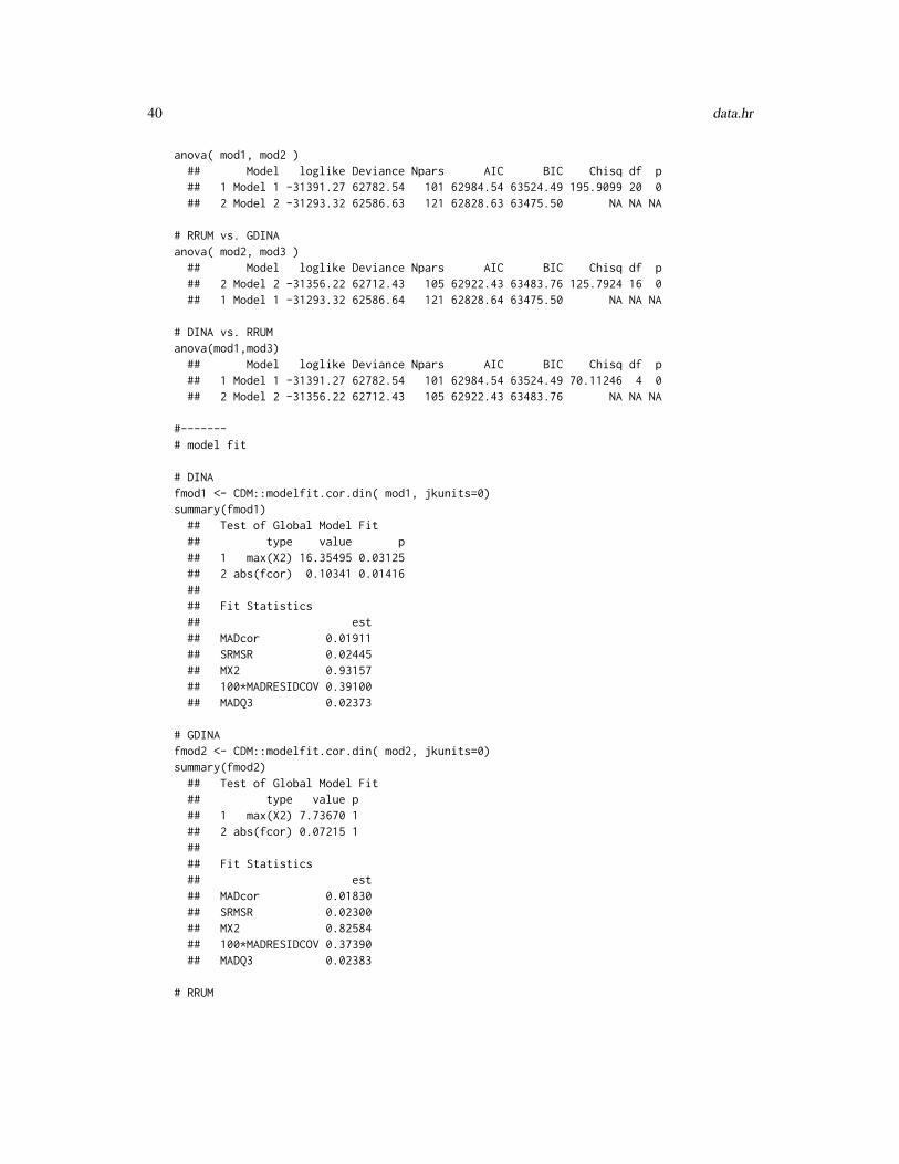
# DINA vs GDINA

40 data.hr

anova( mod1, mod2 )## Model loglike Deviance Npars AIC BIC Chisq df p## 1 Model 1 -31391.27 62782.54 101 62984.54 63524.49 195.9099 20 0## 2 Model 2 -31293.32 62586.63 121 62828.63 63475.50 NA NA NA

# RRUM vs. GDINAanova( mod2, mod3 )


# DINA vs. RRUManova(mod1,mod3)


#-------# model fit

# DINAfmod1 <- CDM::modelfit.cor.din( mod1, jkunits=0)summary(fmod1)


# GDINAfmod2 <- CDM::modelfit.cor.din( mod2, jkunits=0)summary(fmod2)

## Test of Global Model Fit## type value p## 1 max(X2) 7.73670 1## 2 abs(fcor) 0.07215 1#### Fit Statistics## est## MADcor 0.01830## SRMSR 0.02300## MX2 0.82584## 100*MADRESIDCOV 0.37390## MADQ3 0.02383

# RRUM

data.jang 41

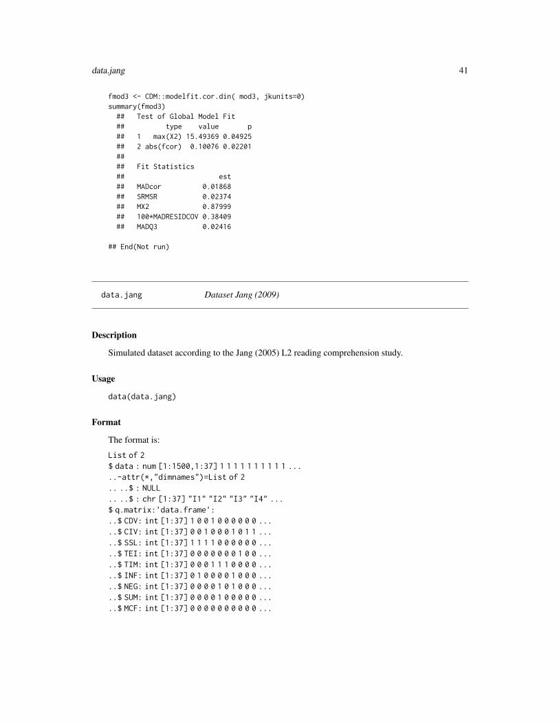
fmod3 <- CDM::modelfit.cor.din( mod3, jkunits=0)summary(fmod3)


## End(Not run)

data.jang Dataset Jang (2009)

Description

Simulated dataset according to the Jang (2005) L2 reading comprehension study.

Usage

data(data.jang)

Format

The format is:

List of 2$ data : num [1:1500,1:37] 1 1 1 1 1 1 1 1 1 1 .....-attr(*,"dimnames")=List of 2.. ..$ : NULL.. ..$ : chr [1:37] "I1" "I2" "I3" "I4" ...$ q.matrix:'data.frame':..$ CDV: int [1:37] 1 0 0 1 0 0 0 0 0 0 .....$ CIV: int [1:37] 0 0 1 0 0 0 1 0 1 1 .....$ SSL: int [1:37] 1 1 1 1 0 0 0 0 0 0 .....$ TEI: int [1:37] 0 0 0 0 0 0 0 1 0 0 .....$ TIM: int [1:37] 0 0 0 1 1 1 0 0 0 0 .....$ INF: int [1:37] 0 1 0 0 0 0 1 0 0 0 .....$ NEG: int [1:37] 0 0 0 0 1 0 1 0 0 0 .....$ SUM: int [1:37] 0 0 0 0 1 0 0 0 0 0 .....$ MCF: int [1:37] 0 0 0 0 0 0 0 0 0 0 ...

42 data.jang

Source

Simulated dataset.

References

Jang, E. E. (2009). Cognitive diagnostic assessment of L2 reading comprehension ability: Validityarguments for Fusion Model application to LanguEdge assessment. Language Testing, 26, 31-73.

Examples

## Not run:data(data.jang, package="CDM")

data <- data.jang$dataq.matrix <- data.jang$q.matrix

#*** Model 1: Reduced RUM modelmod1 <- CDM::gdina( data, q.matrix, rule="RRUM", conv.crit=.001, increment.factor=1.025 )summary(mod1)

#*** Model 2: Additive model (identity link)mod2 <- CDM::gdina( data, q.matrix, rule="ACDM", conv.crit=.001, linkfct="identity" )summary(mod2)

#*** Model 3: DINA modelmod3 <- CDM::gdina( data, q.matrix, rule="DINA", conv.crit=.001 )summary(mod3)

anova(mod1,mod2)## Model loglike Deviance Npars AIC BIC Chisq df p## 1 Model 1 -30315.03 60630.06 153 60936.06 61748.98 88.29627 0 0## 2 Model 2 -30270.88 60541.76 153 60847.76 61660.68 NA NA NA


# RRUMsummary( CDM::modelfit.cor.din( mod1, jkunits=0) )

## type value p## 1 max(X2) 11.79073 0.39645## 2 abs(fcor) 0.09541 0.07422## est## MADcor 0.01834## SRMSR 0.02300## MX2 0.86718## 100*MADRESIDCOV 0.38690## MADQ3 0.02413

# additive model (identity)summary( CDM::modelfit.cor.din( mod2, jkunits=0) )

## type value p

data.melab 43

## 1 max(X2) 9.78958 1.00000## 2 abs(fcor) 0.08770 0.22993## est## MADcor 0.01721## SRMSR 0.02158## MX2 0.69163## 100*MADRESIDCOV 0.36343## MADQ3 0.02423

# DINA modelsummary( CDM::modelfit.cor.din( mod3, jkunits=0) )

## type value p## 1 max(X2) 13.48449 0.16020## 2 abs(fcor) 0.10651 0.01256## est## MADcor 0.01999## SRMSR 0.02495## MX2 0.92820## 100*MADRESIDCOV 0.42226## MADQ3 0.02258

## End(Not run)

data.melab MELAB Data (Li, 2011)

Description

This is a simulated dataset according to the MELAB reading study (Li, 2011; Li & Suen, 2013). Li(2011) investigated the Fusion model (RUM model) for calibrating this dataset. The dataset in thispackage is simulated assuming the reduced RUM model (RRUM).

Usage

data(data.melab)

Format

The format of the dataset is:

List of 3$ data : num [1:2019,1:20] 0 1 0 1 1 0 0 0 1 1 .....-attr(*,"dimnames")=List of 2.. ..$ : NULL.. ..$ : chr [1:20] "I1" "I2" "I3" "I4" ...$ q.matrix :'data.frame':..$ skill1: int [1:20] 1 1 0 0 1 1 0 1 0 1 .....$ skill2: int [1:20] 0 0 0 0 0 0 0 0 0 0 .....$ skill3: int [1:20] 0 0 0 1 0 1 1 0 1 0 .....$ skill4: int [1:20] 1 0 1 0 1 0 0 1 0 1 ...

44 data.melab

$ skill.labels:'data.frame':..$ skill : Factor w/ 4 levels "skill1","skill2",..: 1 2 3 4..$ skill.label: Factor w/ 4 levels "connecting and synthesizing",..: 4 3 2 1

Source

Simulated data according to Li (2011).

References

Li, H. (2011). A cognitive diagnostic analysis of the MELAB reading test. Spaan Fellow, 9, 17-46.

Li, H., & Suen, H. K. (2013). Constructing and validating a Q-matrix for cognitive diagnosticanalyses of a reading test. Educational Assessment, 18, 1-25.

Examples

## Not run:data(data.melab, package="CDM")

data <- data.melab$dataq.matrix <- data.melab$q.matrix

#*** Model 1: Reduced RUM modelmod1 <- CDM::gdina( data, q.matrix, rule="RRUM" )summary(mod1)

#*** Model 2: GDINA modelmod2 <- CDM::gdina( data, q.matrix, rule="GDINA" )summary(mod2)

#*** Model 3: DINA modelmod3 <- CDM::gdina( data, q.matrix, rule="DINA" )summary(mod3)

#*** Model 4: 2PL modelmod4 <- CDM::gdm( data, theta.k=seq(-6,6,len=21), center )summary(mod4)

#----# Model comparisons

#*** RRUM vs. GDINAanova(mod1,mod2)

## Model loglike Deviance Npars AIC BIC Chisq df p## 1 Model 1 -20252.74 40505.48 69 40643.48 41030.60 30.88801 18 0.02966## 2 Model 2 -20237.30 40474.59 87 40648.59 41136.69 NA NA NA

## -> GDINA is not superior to RRUM (according to AIC and BIC)

#*** DINA vs. RRUManova(mod1,mod3)

data.melab 45


## -> RRUM fits the data significantly better than the DINA model

#*** RRUM vs. 2PL (use only AIC and BIC for comparison)anova(mod1,mod4)


## -> RRUM fits the data better than 2PL

#----# Model fit statistics

# RRUMfmod1 <- CDM::modelfit.cor.din( mod1, jkunits=0)summary(fmod1)


## -> not a significant misfit of the RRUM model

# GDINAfmod2 <- CDM::modelfit.cor.din( mod2, jkunits=0)summary(fmod2)


## End(Not run)

46 data.mg

data.mg Large-Scale Dataset with Multiple Groups

Description

Large-scale dataset with multiple groups, survey weights and 11 polytomous items.

Usage

data(data.mg)

Format

A data frame with 38243 observations on the following 14 variables.

idstud Student identifier

group Group identifier

weight Survey weight

I1 Item 1

I2 Item 2

I3 Item 3

I4 Item 4

I5 Item 5

I6 Item 6

I7 Item 7

I8 Item 8

I9 Item 9

I10 Item 10

I11 Item 11

Source

Subsample of a large-scale dataset of 11 survey questions.

Examples

## Not run:library(psych)data(dat.mg, package="CDM")psych::describe( data.mg )

## > psych::describe(data.mg)## var n mean sd median trimmed mad min max## idstud 1 38243 1039653.91 19309.80 1037899.00 1039927.73 30240.59 1007168.00 1069949.00## group 2 38243 8.06 4.07 7.00 8.06 5.93 2.00 14.00

data.pgdina 47

## weight 3 38243 28.76 19.25 31.88 27.92 19.12 0.79 191.89## I1 4 37665 0.88 0.32 1.00 0.98 0.00 0.00 1.00## I2 5 37639 0.93 0.25 1.00 1.00 0.00 0.00 1.00## I3 6 37473 0.76 0.43 1.00 0.83 0.00 0.00 1.00## I4 7 37687 1.88 0.39 2.00 2.00 0.00 0.00 2.00## I5 8 37638 1.36 0.75 2.00 1.44 0.00 0.00 2.00## I6 9 37587 1.05 0.82 1.00 1.06 1.48 0.00 2.00## I7 10 37576 1.55 0.85 2.00 1.57 1.48 0.00 3.00## I8 11 37044 0.45 0.50 0.00 0.44 0.00 0.00 1.00## I9 12 37249 0.48 0.50 0.00 0.47 0.00 0.00 1.00## I10 13 37318 0.63 0.48 1.00 0.66 0.00 0.00 1.00## I11 14 37412 1.35 0.80 1.00 1.35 1.48 0.00 3.00

## End(Not run)

data.pgdina Dataset for Polytomous GDINA Model

Description

Dataset for the estimation of the polytomous GDINA model.

Usage

data(data.pgdina)

Format

The dataset is a list with the item response data and the Q-matrix. The format is:

List of 2$ dat : num [1:1000,1:30] 1 1 1 1 1 0 1 1 1 1 .....-attr(*,"dimnames")=List of 2.. ..$ : NULL.. ..$ : chr [1:30] "I1" "I2" "I3" "I4" ...$ q.matrix: num [1:30,1:5] 1 0 0 0 0 1 0 0 0 2 ...

Details

The dataset was simulated by the following R code:

set.seed(89)# define Q-matrixQmatrix <-matrix(c(1,0,0,0,0,0,1,0,0,0,0,0,1,0,0,0,0,0,1,0,0,0,0,0,1,1,2,0,0,0,0,1,2,0,0,0,0,1,2,0,0,0,0,1,1,2,0,0,0,1,2,2,0,1,0,2,1,0,0,1,1,0,2,2,0,0,2,1,0,1,0,0,2,2,1,2,0,0,0,0,0,2,0,0,0,0,0,2,0,0,0,0,0,2,0,0,0,0,0,1,2,0,2,0,0,0,2,0,2,0,0,0,2,0,1,2,0,0,2,0,0,2,0,0,1,1,0,0,1,1,0,1,1,1,0,1,1,1,0,0,0,1,0,1,1,1,0,1,0,1),nrow=30,ncol=5,byrow=TRUE )

48 data.pisa00R

# define covariance matrix between attributesSigma <-matrix(c(1,.6,.6,.3,.3,.6,1,.6,.3,.3,.6,.6,1,.3,.3,.3,.3,.3,1,.8,.3,.3,.3,.8,1),5,5,byrow=TRUE )# define thresholds for attributesq1 <-c( -.5,.9 ) # attributes 1,...,4q2 <-c(0) # attribute 5# number of personsN <-1000# simulate latent attributesalpha1 <-mvrnorm(n=N,mu=rep(0,5),Sigma=Sigma)alpha <-0*alpha1for (aa in 1:4){alpha[ alpha1[,aa] > q1[1],aa ] <-1alpha[ alpha1[,aa] > q1[2],aa ] <-2}aa <-5 ; alpha[ alpha1[,aa] > q2[1],aa ] <-1# define item parametersguess <-c(.07,.01,.34,.07,.11,.23,.27,.07,.08,.34,.19,.19,.25,.04,.34,.03,.29,.05,.01,.17,.15,.35,.19,.16,.08,.18,.19,.07,.17,.34)slip <-c(0,.11,.14,.09,.03,.09,.03,.1,.14,.07,.06,.19,.09,.19,.07,.08,.16,.18,.16,.02,.11,.12,.16,.14,.18,.01,.18,.14,.05,.18)# simulate item responsesI <-30 # number of itemsdat <-latresp <-matrix( 0,N,I,byrow=TRUE)for (ii in 1:I){# ii <-2# latent response matrixlatresp[,ii] <-1*( rowMeans( alpha >=matrix( Qmatrix[ ii,],nrow=N,ncol=5,byrow=TRUE ) )==1 )# response probabilityprob <-ifelse( latresp[,ii]==1,1-slip[ii],guess[ii] )# simulate item responsesdat[,ii] <-1 * ( runif(N ) < prob )}colnames(dat) <-paste0("I",1:I)

References


data.pisa00R PISA 2000 Reading Study (Chen & de la Torre, 2014)

data.pisa00R 49

Description

This is a sub-dataset of the PISA 2000 of German students including 26 items of the reading test.The 26 items was analyzed in Chen and de la Torre (2014) and a subset of 20 items was analyzedin Chen and Chen (2016).

Usage

data(data.pisa00R.ct)data(data.pisa00R.cc)

Format

• The format of the dataset data.pisa00R.ct (Chen & de la Torre, 2014) is:List of 3$ data :'data.frame': 1095 obs. of 111 variables:.. [list output truncated]$ q.matrix: num [1:26,1:8] 0 1 0 0 0 1 0 0 0 1 .....-attr(*,"dimnames")=List of 2$ skills : chr [1:8] "Locating information" ...

• The format of the dataset data.pisa00R.cc (Q-matrix in Chen and Chen, 2016)List of 2$ q.matrix:'data.frame': 20 obs. of 5 variables:..$ A1: num [1:20] 1 1 0 0 1 1 1 0 0 0 .....$ A2: num [1:20] 0 0 0 1 0 1 1 1 1 1 .....$ A3: num [1:20] 1 1 0 1 1 0 1 0 1 0 .....$ A4: num [1:20] 0 1 1 1 0 0 0 0 0 0 .....$ A5: num [1:20] 0 0 1 0 0 0 0 1 0 1 ...$ skills : Named chr [1:5] "Identifying Explicit Information" .....-attr(*,"names")=chr [1:5] "A1" "A2" "A3" "A4" ...

References

Chen, H., & Chen, J. (2016). Exploring reading comprehension skill relationships through theG-DINA model. Educational Psychology, 36(6), 1049-1064.

Chen, J., & de la Torre, J. (2014). A procedure for diagnostically modeling extant large-scale assess-ment data: the case of the programme for international student assessment in reading. Psychology,5(18), 1967-1978.

Examples

############################################################################## EXAMPLE 1: PISA items from Chen and de la Torre (2014)# dichotomize item responses#############################################################################

data(data.pisa00R.ct, package="CDM")

50 data.sda6

dat <- data.pisa00R.ct$dataQ <- data.pisa00R.ct$q.matrixresp <- dat[, rownames(Q)]

#** extract item-wise maximummaxK <- apply( resp, 2, max, na.rm=TRUE )#** dichotomize response dataresp1 <- respfor (ii in seq(1,ncol(resp)) ){

resp1[,ii] <- 1 * ( resp[,ii]==maxK[ii] )}

data.sda6 Dataset SDA6 (Jurich & Bradshaw, 2014)

Description

This is a simulated dataset of the SDA6 study according to informations given in Jurich and Brad-shaw (2014).

Usage

data(data.sda6)

Format

The datasets contains 17 items observed at 1710 students.

The format is:

List of 2$ data : num [1:1710,1:17] 0 1 0 1 0 0 0 0 1 0 .....-attr(*,"dimnames")=List of 2.. ..$ : NULL.. ..$ : chr [1:17] "MCM01" "MCM03" "MCM13" "MCM17" ...$ q.matrix:'data.frame':..$ CM: int [1:17] 1 1 1 1 0 0 0 0 0 0 .....$ II: int [1:17] 0 0 0 0 1 1 1 1 0 0 .....$ PP: int [1:17] 0 0 0 0 0 0 0 0 1 1 .....$ DG: int [1:17] 0 0 0 0 0 0 0 0 0 0 ...

The meaning of the skills is

CM – Critique Methods

II – Identify Improvements

PP – Protect Participants

DG – Discern Generalizability

data.sda6 51

Source

Simulated data

References

Jurich, D. P., & Bradshaw, L. P. (2014). An illustration of diagnostic classification modeling instudent learning outcomes assessment. International Journal of Testing, 14, 49-72.

Examples

## Not run:data(data.sda6, package="CDM")

data <- data.sda6$dataq.matrix <- data.sda6$q.matrix

#*** Model 1a: LCDM with gdinamod1a <- CDM::gdina( data, q.matrix, rule="ACDM", linkfct="logit",

reduced.skillspace=FALSE )summary(mod1a)

#*** Model 1b: estimate LCDM with gdmmod1b <- CDM::gdm( data, q.matrix=q.matrix, theta.k=c(0,1) )summary(mod1b)

#*** Model 2: LCDM with hierarchy II > CMB <- "II > CM"ss2 <- CDM::skillspace.hierarchy(B=B, skill.names=colnames(q.matrix ) )mod2 <- CDM::gdina( data, q.matrix, rule="ACDM", linkfct="logit",

skillclasses=ss2$skillspace.reduced,reduced.skillspace=FALSE )

summary(mod2)

#*** Model 3: LCDM with hierarchy II > CM and DG > CMB <- "II > CM

DG > CM"ss2 <- CDM::skillspace.hierarchy(B=B, skill.names=colnames(q.matrix ) )mod3 <- CDM::gdina( data, q.matrix, rule="ACDM", linkfct="logit",

skillclasses=ss2$skillspace.reduced,reduced.skillspace=FALSE )

summary(mod3)

# model comparisonsanova(mod1a,mod2)anova(mod1a,mod3)# model fitsummary( CDM::modelfit.cor.din(mod1a))summary( CDM::modelfit.cor.din(mod2) )summary( CDM::modelfit.cor.din(mod3) )

## End(Not run)

52 data.Students

data.Students Dataset Student Questionnaire

Description

This dataset contains item responses of students at a scale of cultural activities (act), mathematicsself concept (sc) and mathematics joyment (mj).

Usage

data(data.Students)

Format

A data frame with 2400 observations on the following 15 variables.

urban Urbanization level: 1=town, 0=otherwise

female A dummy variable for female student

act1 Visit a museum (0=never, 1=once or twice a year, 2=more than twice a year)

act2 Visit a theater or classical concert (0,1,2)

act3 Visit a rock or pop concert (0,1,2)

act4 Visit a cinema (0,1,2)

act5 Visit a public library (0,1,2)

sc1 Item 1 self concept "I am usually good at math." (0=do not agree at all, 1=rather do not agree,2=rather agree, 3=completely agree)

sc2 Item 2 self concept: "Mathematics is harder for me than many of my classmates." (0,1,2,3)(reversed)

sc3 Item 3 self concept: "I am just not good at math." (0,1,2,3) (reversed)

sc4 Item 4 self concept: "I’m learning fast in math." (0,1,2,3)

mj1 Item 1 mathematics joyment: "I would like more math at school." (0,1,2,3)

mj2 Item 2 mathematics joyment: "I like to learn mathematics." (0,1,2,3)

mj3 Item 3 mathematics joyment: "Math is boring." (0,1,2,3) (reversed)

mj4 Item 4 mathematics joyment: "I like math." (0,1,2,3)

Source

Subsample of students from an Austrian survey of 8th grade students.

data.timss03.G8.su 53

Examples

## Not run:library(psych)data(data.Students, package="CDM")psych::describe(data.Students)

## var n mean sd median trimmed mad min max range skew kurtosis se## urban 1 2400 0.31 0.46 0.0 0.27 0.00 0 1 1 0.81 -1.34 0.01## female 2 2400 0.51 0.50 1.0 0.51 0.00 0 1 1 -0.03 -2.00 0.01## act1 3 2248 0.65 0.73 0.5 0.56 0.74 0 2 2 0.64 -0.88 0.02## act2 4 2230 0.47 0.69 0.0 0.34 0.00 0 2 2 1.13 -0.06 0.01## act3 5 2218 0.33 0.60 0.0 0.21 0.00 0 2 2 1.62 1.48 0.01## act4 6 2342 1.35 0.76 2.0 1.44 0.00 0 2 2 -0.69 -0.96 0.02## act5 7 2223 0.52 0.74 0.0 0.40 0.00 0 2 2 1.05 -0.41 0.02## sc1 8 2352 0.96 0.80 1.0 0.91 1.48 0 3 3 0.45 -0.39 0.02## sc2 9 2347 0.90 0.88 1.0 0.81 1.48 0 3 3 0.66 -0.41 0.02## sc3 10 2335 0.86 0.96 1.0 0.73 1.48 0 3 3 0.84 -0.35 0.02## sc4 11 2337 1.29 0.90 1.0 1.24 1.48 0 3 3 0.24 -0.71 0.02## mj1 12 2351 2.26 0.82 2.0 2.37 1.48 0 3 3 -0.94 0.28 0.02## mj2 13 2345 1.89 0.91 2.0 1.95 1.48 0 3 3 -0.35 -0.80 0.02## mj3 14 2334 1.47 1.02 1.0 1.47 1.48 0 3 3 0.10 -1.11 0.02## mj4 15 2346 1.59 0.99 2.0 1.62 1.48 0 3 3 -0.03 -1.06 0.02

## End(Not run)

data.timss03.G8.su TIMSS 2003 Mathematics 8th Grade (Su et al., 2013)

Description

This is a dataset with a subset of 23 Mathematics items from TIMSS 2003 items used in Su, Choi,Lee, Choi and McAninch (2013).

Usage

data(data.timss03.G8.su)

Format

The data contains scored item responses (data), the Q-matrix (q.matrix) and further item infor-mations (iteminfo).

The format is

List of 3$ data :'data.frame':..$ idstud : num [1:757] 1e+07 1e+07 1e+07 1e+07 1e+07 .....$ idbook : num [1:757] 1 1 1 1 1 1 1 1 1 1 .....$ M012001 : num [1:757] 0 1 0 0 1 0 1 0 0 0 .....$ M012002 : num [1:757] 1 1 0 1 0 0 1 1 1 1 .....$ M012004 : num [1:757] 0 1 1 1 1 0 1 1 0 0 ...

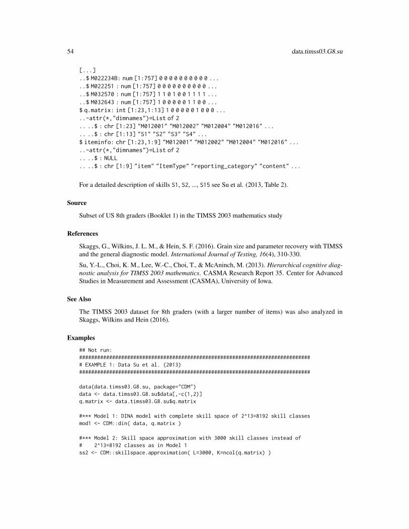
54 data.timss03.G8.su

[...]..$ M022234B: num [1:757] 0 0 0 0 0 0 0 0 0 0 .....$ M022251 : num [1:757] 0 0 0 0 0 0 0 0 0 0 .....$ M032570 : num [1:757] 1 1 0 1 0 0 1 1 1 1 .....$ M032643 : num [1:757] 1 0 0 0 0 0 1 1 0 0 ...$ q.matrix: int [1:23,1:13] 1 0 0 0 0 0 1 0 0 0 .....-attr(*,"dimnames")=List of 2.. ..$ : chr [1:23] "M012001" "M012002" "M012004" "M012016" ..... ..$ : chr [1:13] "S1" "S2" "S3" "S4" ...$ iteminfo: chr [1:23,1:9] "M012001" "M012002" "M012004" "M012016" .....-attr(*,"dimnames")=List of 2.. ..$ : NULL.. ..$ : chr [1:9] "item" "ItemType" "reporting_category" "content" ...

For a detailed description of skills S1, S2, ..., S15 see Su et al. (2013, Table 2).

Source

Subset of US 8th graders (Booklet 1) in the TIMSS 2003 mathematics study

References

Skaggs, G., Wilkins, J. L. M., & Hein, S. F. (2016). Grain size and parameter recovery with TIMSSand the general diagnostic model. International Journal of Testing, 16(4), 310-330.

Su, Y.-L., Choi, K. M., Lee, W.-C., Choi, T., & McAninch, M. (2013). Hierarchical cognitive diag-nostic analysis for TIMSS 2003 mathematics. CASMA Research Report 35. Center for AdvancedStudies in Measurement and Assessment (CASMA), University of Iowa.

See Also

The TIMSS 2003 dataset for 8th graders (with a larger number of items) was also analyzed inSkaggs, Wilkins and Hein (2016).

Examples

## Not run:############################################################################## EXAMPLE 1: Data Su et al. (2013)#############################################################################

data(data.timss03.G8.su, package="CDM")data <- data.timss03.G8.su$data[,-c(1,2)]q.matrix <- data.timss03.G8.su$q.matrix

#*** Model 1: DINA model with complete skill space of 2^13=8192 skill classesmod1 <- CDM::din( data, q.matrix )

#*** Model 2: Skill space approximation with 3000 skill classes instead of# 2^13=8192 classes as in Model 1ss2 <- CDM::skillspace.approximation( L=3000, K=ncol(q.matrix) )

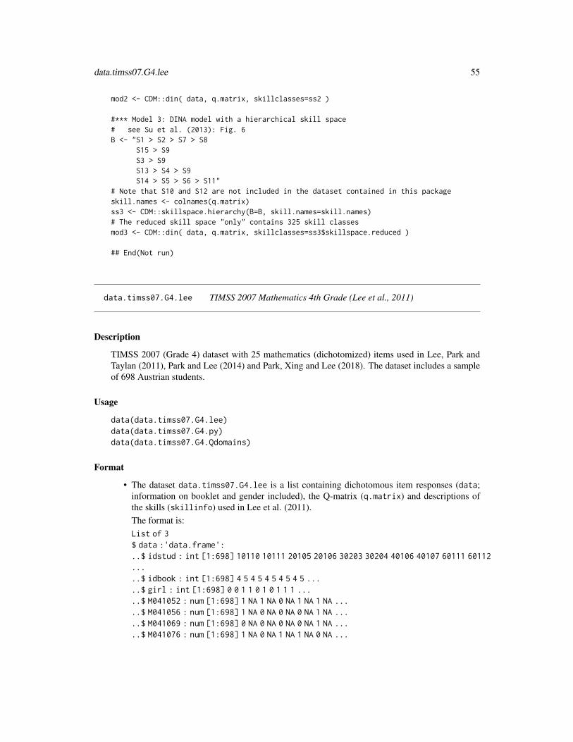
data.timss07.G4.lee 55

mod2 <- CDM::din( data, q.matrix, skillclasses=ss2 )

#*** Model 3: DINA model with a hierarchical skill space# see Su et al. (2013): Fig. 6B <- "S1 > S2 > S7 > S8

S15 > S9S3 > S9S13 > S4 > S9S14 > S5 > S6 > S11"

# Note that S10 and S12 are not included in the dataset contained in this packageskill.names <- colnames(q.matrix)ss3 <- CDM::skillspace.hierarchy(B=B, skill.names=skill.names)# The reduced skill space "only" contains 325 skill classesmod3 <- CDM::din( data, q.matrix, skillclasses=ss3$skillspace.reduced )

## End(Not run)

data.timss07.G4.lee TIMSS 2007 Mathematics 4th Grade (Lee et al., 2011)

Description

TIMSS 2007 (Grade 4) dataset with 25 mathematics (dichotomized) items used in Lee, Park andTaylan (2011), Park and Lee (2014) and Park, Xing and Lee (2018). The dataset includes a sampleof 698 Austrian students.

Usage

data(data.timss07.G4.lee)data(data.timss07.G4.py)data(data.timss07.G4.Qdomains)

Format

• The dataset data.timss07.G4.lee is a list containing dichotomous item responses (data;information on booklet and gender included), the Q-matrix (q.matrix) and descriptions ofthe skills (skillinfo) used in Lee et al. (2011).The format is:List of 3$ data :'data.frame':..$ idstud : int [1:698] 10110 10111 20105 20106 30203 30204 40106 40107 60111 60112.....$ idbook : int [1:698] 4 5 4 5 4 5 4 5 4 5 .....$ girl : int [1:698] 0 0 1 1 0 1 0 1 1 1 .....$ M041052 : num [1:698] 1 NA 1 NA 0 NA 1 NA 1 NA .....$ M041056 : num [1:698] 1 NA 0 NA 0 NA 0 NA 1 NA .....$ M041069 : num [1:698] 0 NA 0 NA 0 NA 0 NA 1 NA .....$ M041076 : num [1:698] 1 NA 0 NA 1 NA 1 NA 0 NA ...

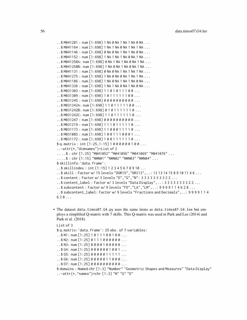
56 data.timss07.G4.lee

..$ M041281 : num [1:698] 1 NA 0 NA 1 NA 1 NA 0 NA ...

..$ M041164 : num [1:698] 1 NA 1 NA 0 NA 1 NA 1 NA ...

..$ M041146 : num [1:698] 0 NA 0 NA 1 NA 1 NA 0 NA ...

..$ M041152 : num [1:698] 1 NA 1 NA 1 NA 0 NA 1 NA ...

..$ M041258A: num [1:698] 0 NA 1 NA 1 NA 0 NA 1 NA ...

..$ M041258B: num [1:698] 1 NA 0 NA 1 NA 0 NA 1 NA ...

..$ M041131 : num [1:698] 0 NA 0 NA 1 NA 1 NA 1 NA ...

..$ M041275 : num [1:698] 1 NA 0 NA 0 NA 1 NA 1 NA ...

..$ M041186 : num [1:698] 1 NA 0 NA 1 NA 1 NA 0 NA ...

..$ M041336 : num [1:698] 1 NA 1 NA 0 NA 1 NA 0 NA ...

..$ M031303 : num [1:698] 1 1 0 1 0 1 1 1 0 0 ...

..$ M031309 : num [1:698] 1 0 1 1 1 1 1 1 0 0 ...

..$ M031245 : num [1:698] 0 0 0 0 0 0 0 0 0 0 ...

..$ M031242A: num [1:698] 1 1 0 1 1 1 1 1 0 0 ...

..$ M031242B: num [1:698] 0 1 0 1 1 1 1 1 1 0 ...

..$ M031242C: num [1:698] 1 1 0 1 1 1 1 1 1 0 ...

..$ M031247 : num [1:698] 0 0 0 0 0 0 0 0 0 0 ...

..$ M031219 : num [1:698] 1 1 1 0 1 1 1 1 1 0 ...

..$ M031173 : num [1:698] 1 1 0 0 0 1 1 1 1 0 ...

..$ M031085 : num [1:698] 1 0 0 1 1 1 0 0 0 1 ...

..$ M031172 : num [1:698] 1 0 0 1 1 1 1 1 1 0 ...$ q.matrix : int [1:25,1:15] 1 0 0 0 0 0 0 1 0 0 .....-attr(*,"dimnames")=List of 2.. ..$ : chr [1:25] "M041052" "M041056" "M041069" "M041076" ..... ..$ : chr [1:15] "NWN01" "NWN02" "NWN03" "NWN04" ...$ skillinfo:'data.frame':..$ skillindex : int [1:15] 1 2 3 4 5 6 7 8 9 10 .....$ skill : Factor w/ 15 levels "DOR15","DRI13",..: 12 13 14 15 8 9 10 11 4 6 .....$ content : Factor w/ 3 levels "D","G","N": 3 3 3 3 3 3 3 3 2 2 .....$ content_label : Factor w/ 3 levels "Data Display",..: 3 3 3 3 3 3 3 3 2 2 .....$ subcontent : Factor w/ 9 levels "FD","LA","LM",..: 9 9 9 9 1 1 4 6 2 8 .....$ subcontent_label: Factor w/ 9 levels "Fractions and Decimals",..: 9 9 9 9 1 1 46 2 8 ...

• The dataset data.timss07.G4.py uses the same items as data.timss07.G4.lee but em-ploys a simplified Q-matrix with 7 skills. This Q-matrix was used in Park and Lee (2014) andPark et al. (2018).

List of 3$ q.matrix:'data.frame': 25 obs. of 7 variables:..$ N1: num [1:25] 1 0 1 1 1 0 0 1 0 0 .....$ N2: num [1:25] 0 1 1 1 0 0 0 0 0 0 .....$ N3: num [1:25] 0 0 0 0 1 0 0 0 0 0 .....$ G4: num [1:25] 0 0 0 0 0 0 1 0 0 1 .....$ G5: num [1:25] 0 0 0 0 0 1 1 1 1 1 .....$ G6: num [1:25] 0 0 0 0 0 1 1 0 0 0 .....$ D7: num [1:25] 0 0 0 0 0 0 0 0 0 0 ...$ domains : Named chr [1:3] "Number" "Geometric Shapes and Measures" "Data Display"..-attr(*,"names")=chr [1:3] "N" "G" "D"

data.timss07.G4.lee 57

$ skills : Named chr [1:7] "Whole Numbers" .....-attr(*,"names")=chr [1:7] "N1" "N2" "N3" "G4" ...

• The Q-matrix data.timss07.G4.Qdomains is a simplification of data.timss07.G4.py$q.matrixto 3 domains and involves a simple structure of skills.num [1:25,1:3] 1 1 1 1 1 0 0 1 0 0 ...-attr(*,"dimnames")=List of 2..$ : chr [1:25] "M041052" "M041056" "M041069" "M041076" .....$ : chr [1:3] "N" "G" "D"

Source

TIMSS 2007 study, 4th Grade, Austrian sample on booklets 4 and 5

References

Lee, Y. S., Park, Y. S., & Taylan, D. (2011). A cognitive diagnostic modeling of attribute masteryin Massachusetts, Minnesota, and the US national sample using the TIMSS 2007. InternationalJournal of Testing, 11, 144-177.

Park, Y. S., & Lee, Y. S. (2014). An extension of the DINA model using covariates: Examiningfactors affecting response probability and latent classification. Applied Psychological Measurement,38(5), 376-390.

Park, Y. S., Xing, K., & Lee, Y. S. (2018). Explanatory cognitive diagnostic models: Incorporatinglatent and observed predictors. Applied Psychological Measurement, 42(5), 376-392.

Yamaguchi, K., & Okada, K. (2018). Comparison among cognitive diagnostic models for theTIMSS 2007 fourth grade mathematics assessment. PloS ONE, 13(2), e0188691.

See Also

A comparison of several countries based on the 25 items is conducted in Yamaguchi and Okada(2018).

Examples

## Not run:############################################################################## EXAMPLE 1: DINA model Lee et al. (2011) - 15 skills#############################################################################

data(data.timss07.G4.lee, package="CDM")dat <- data.timss07.G4.lee$dataq.matrix <- data.timss07.G4.lee$q.matrix# extract itemsitems <- grep( "M0", colnames(dat), value=TRUE )

#*** Model 1: estimate DINA modelmod1 <- CDM::din( dat[,items], q.matrix )summary(mod1)

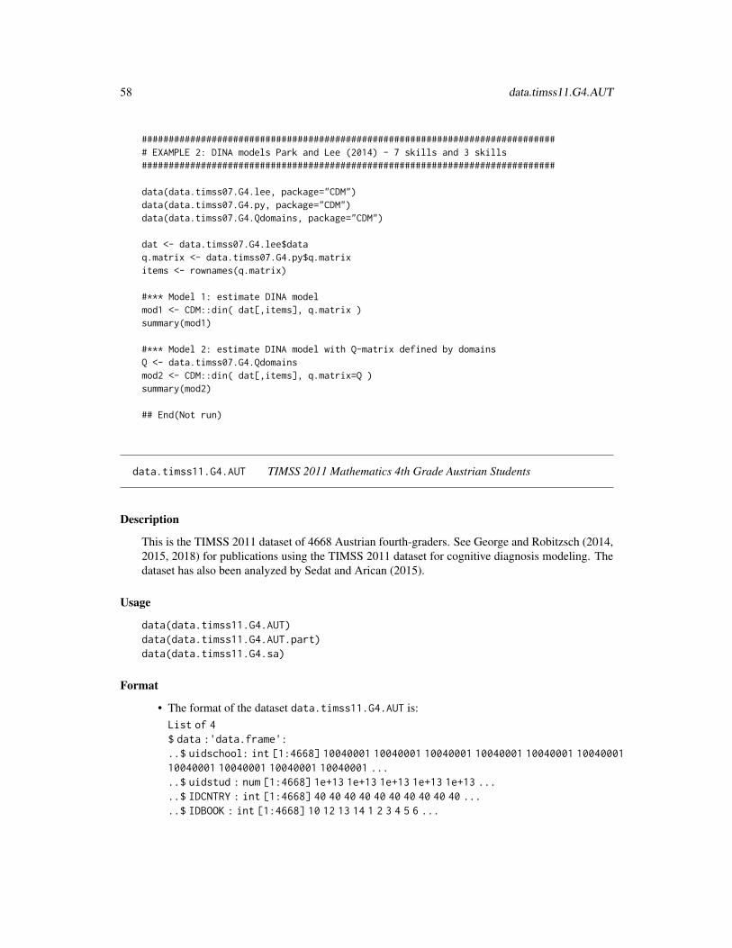
58 data.timss11.G4.AUT

############################################################################## EXAMPLE 2: DINA models Park and Lee (2014) - 7 skills and 3 skills#############################################################################

data(data.timss07.G4.lee, package="CDM")data(data.timss07.G4.py, package="CDM")data(data.timss07.G4.Qdomains, package="CDM")

dat <- data.timss07.G4.lee$dataq.matrix <- data.timss07.G4.py$q.matrixitems <- rownames(q.matrix)

#*** Model 1: estimate DINA modelmod1 <- CDM::din( dat[,items], q.matrix )summary(mod1)

#*** Model 2: estimate DINA model with Q-matrix defined by domainsQ <- data.timss07.G4.Qdomainsmod2 <- CDM::din( dat[,items], q.matrix=Q )summary(mod2)

## End(Not run)

data.timss11.G4.AUT TIMSS 2011 Mathematics 4th Grade Austrian Students

Description

This is the TIMSS 2011 dataset of 4668 Austrian fourth-graders. See George and Robitzsch (2014,2015, 2018) for publications using the TIMSS 2011 dataset for cognitive diagnosis modeling. Thedataset has also been analyzed by Sedat and Arican (2015).

Usage

data(data.timss11.G4.AUT)data(data.timss11.G4.AUT.part)data(data.timss11.G4.sa)

Format

• The format of the dataset data.timss11.G4.AUT is:List of 4$ data :'data.frame':..$ uidschool: int [1:4668] 10040001 10040001 10040001 10040001 10040001 1004000110040001 10040001 10040001 10040001 .....$ uidstud : num [1:4668] 1e+13 1e+13 1e+13 1e+13 1e+13 .....$ IDCNTRY : int [1:4668] 40 40 40 40 40 40 40 40 40 40 .....$ IDBOOK : int [1:4668] 10 12 13 14 1 2 3 4 5 6 ...

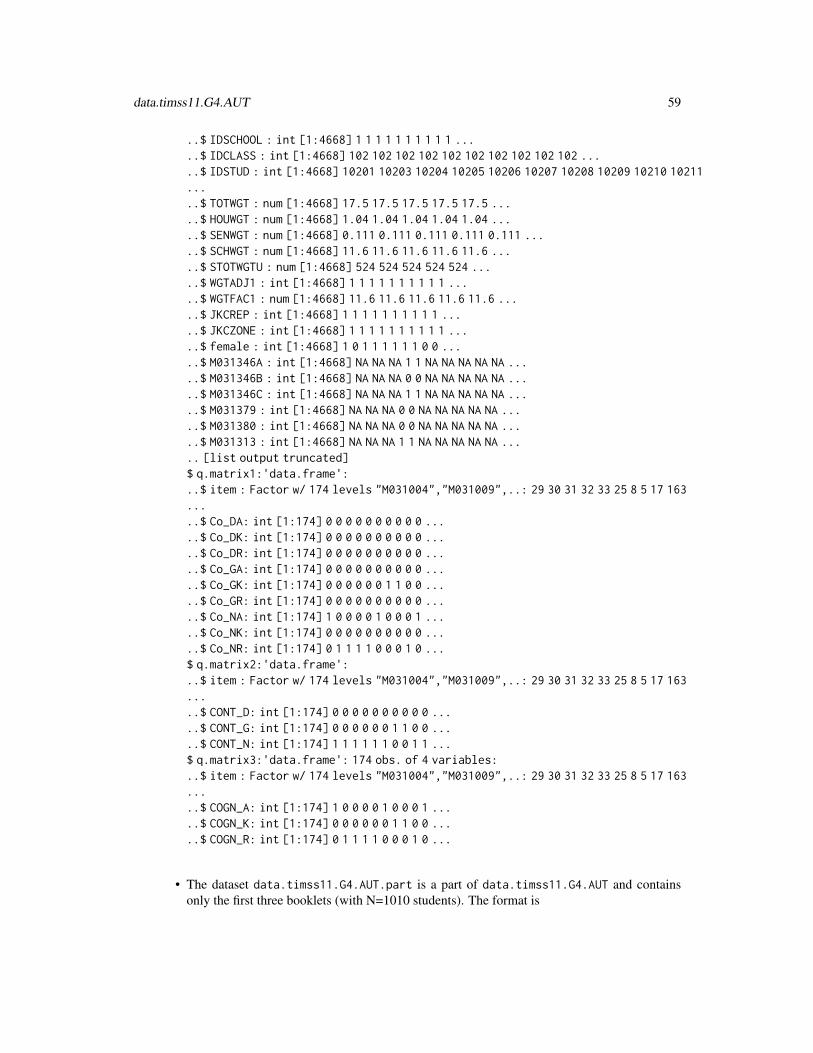
data.timss11.G4.AUT 59

..$ IDSCHOOL : int [1:4668] 1 1 1 1 1 1 1 1 1 1 ...

..$ IDCLASS : int [1:4668] 102 102 102 102 102 102 102 102 102 102 ...

..$ IDSTUD : int [1:4668] 10201 10203 10204 10205 10206 10207 10208 10209 10210 10211

...

..$ TOTWGT : num [1:4668] 17.5 17.5 17.5 17.5 17.5 ...

..$ HOUWGT : num [1:4668] 1.04 1.04 1.04 1.04 1.04 ...

..$ SENWGT : num [1:4668] 0.111 0.111 0.111 0.111 0.111 ...

..$ SCHWGT : num [1:4668] 11.6 11.6 11.6 11.6 11.6 ...

..$ STOTWGTU : num [1:4668] 524 524 524 524 524 ...

..$ WGTADJ1 : int [1:4668] 1 1 1 1 1 1 1 1 1 1 ...

..$ WGTFAC1 : num [1:4668] 11.6 11.6 11.6 11.6 11.6 ...

..$ JKCREP : int [1:4668] 1 1 1 1 1 1 1 1 1 1 ...

..$ JKCZONE : int [1:4668] 1 1 1 1 1 1 1 1 1 1 ...

..$ female : int [1:4668] 1 0 1 1 1 1 1 1 0 0 ...

..$ M031346A : int [1:4668] NA NA NA 1 1 NA NA NA NA NA ...

..$ M031346B : int [1:4668] NA NA NA 0 0 NA NA NA NA NA ...

..$ M031346C : int [1:4668] NA NA NA 1 1 NA NA NA NA NA ...

..$ M031379 : int [1:4668] NA NA NA 0 0 NA NA NA NA NA ...



.. [list output truncated]$ q.matrix1:'data.frame':..$ item : Factor w/ 174 levels "M031004","M031009",..: 29 30 31 32 33 25 8 5 17 163.....$ Co_DA: int [1:174] 0 0 0 0 0 0 0 0 0 0 .....$ Co_DK: int [1:174] 0 0 0 0 0 0 0 0 0 0 .....$ Co_DR: int [1:174] 0 0 0 0 0 0 0 0 0 0 .....$ Co_GA: int [1:174] 0 0 0 0 0 0 0 0 0 0 .....$ Co_GK: int [1:174] 0 0 0 0 0 0 1 1 0 0 .....$ Co_GR: int [1:174] 0 0 0 0 0 0 0 0 0 0 .....$ Co_NA: int [1:174] 1 0 0 0 0 1 0 0 0 1 .....$ Co_NK: int [1:174] 0 0 0 0 0 0 0 0 0 0 .....$ Co_NR: int [1:174] 0 1 1 1 1 0 0 0 1 0 ...$ q.matrix2:'data.frame':..$ item : Factor w/ 174 levels "M031004","M031009",..: 29 30 31 32 33 25 8 5 17 163.....$ CONT_D: int [1:174] 0 0 0 0 0 0 0 0 0 0 .....$ CONT_G: int [1:174] 0 0 0 0 0 0 1 1 0 0 .....$ CONT_N: int [1:174] 1 1 1 1 1 1 0 0 1 1 ...$ q.matrix3:'data.frame': 174 obs. of 4 variables:..$ item : Factor w/ 174 levels "M031004","M031009",..: 29 30 31 32 33 25 8 5 17 163.....$ COGN_A: int [1:174] 1 0 0 0 0 1 0 0 0 1 .....$ COGN_K: int [1:174] 0 0 0 0 0 0 1 1 0 0 .....$ COGN_R: int [1:174] 0 1 1 1 1 0 0 0 1 0 ...

• The dataset data.timss11.G4.AUT.part is a part of data.timss11.G4.AUT and containsonly the first three booklets (with N=1010 students). The format is

60 data.timss11.G4.AUT

List of 4$ data :'data.frame': 1010 obs. of 109 variables:..$ uidschool: int [1:1010] 10040001 10040001 10040001 10040001 .....$ uidstud : num [1:1010] 1e+13 1e+13 1e+13 1e+13 1e+13 .....$ IDCNTRY : int [1:1010] 40 40 40 40 40 40 40 40 40 40 .....$ IDBOOK : int [1:1010] 1 2 3 1 2 1 2 3 1 2 .....$ IDSCHOOL : int [1:1010] 1 1 1 1 1 2 2 2 3 3 .....$ IDCLASS : int [1:1010] 102 102 102 102 102 .....$ IDSTUD : int [1:1010] 10206 10207 10208 10220 .....$ TOTWGT : num [1:1010] 17.5 17.5 17.5 17.5 17.5 .....$ HOUWGT : num [1:1010] 1.04 1.04 1.04 1.04 1.04 .....$ SENWGT : num [1:1010] 0.111 0.111 0.111 0.111 0.111 .....$ SCHWGT : num [1:1010] 11.6 11.6 11.6 11.6 11.6 .....$ STOTWGTU : num [1:1010] 524 524 524 524 524 .....$ WGTADJ1 : int [1:1010] 1 1 1 1 1 1 1 1 1 1 .....$ WGTFAC1 : num [1:1010] 11.6 11.6 11.6 11.6 11.6 .....$ JKCREP : int [1:1010] 1 1 1 1 1 0 0 0 0 0 .....$ JKCZONE : int [1:1010] 1 1 1 1 1 1 1 1 2 2 .....$ female : int [1:1010] 1 1 1 1 0 1 1 1 1 1 .....$ M031346A : int [1:1010] 1 NA NA 1 NA 1 NA NA 1 NA .....$ M031346B : int [1:1010] 0 NA NA 1 NA 0 NA NA 0 NA .....$ M031346C : int [1:1010] 1 NA NA 0 NA 0 NA NA 0 NA .....$ M031379 : int [1:1010] 0 NA NA 0 NA 0 NA NA 1 NA .....$ M031380 : int [1:1010] 0 NA NA 0 NA 0 NA NA 0 NA .....$ M031313 : int [1:1010] 1 NA NA 0 NA 1 NA NA 0 NA .....$ M031083 : int [1:1010] 1 NA NA 1 NA 1 NA NA 1 NA .....$ M031071 : int [1:1010] 0 NA NA 0 NA 1 NA NA 0 NA .....$ M031185 : int [1:1010] 0 NA NA 1 NA 0 NA NA 0 NA .....$ M051305 : int [1:1010] 1 1 NA 1 0 0 0 NA 0 1 .....$ M051091 : int [1:1010] 1 1 NA 1 1 1 1 NA 1 0 ..... [list output truncated]$ q.matrix1:'data.frame': 47 obs. of 10 variables:..$ item : Factor w/ 174 levels "M031004","M031009",..: 29 30 31 32 33 25 8 5 17 163.....$ Co_DA: int [1:47] 0 0 0 0 0 0 0 0 0 0 .....$ Co_DK: int [1:47] 0 0 0 0 0 0 0 0 0 0 .....$ Co_DR: int [1:47] 0 0 0 0 0 0 0 0 0 0 .....$ Co_GA: int [1:47] 0 0 0 0 0 0 0 0 0 0 .....$ Co_GK: int [1:47] 0 0 0 0 0 0 1 1 0 0 .....$ Co_GR: int [1:47] 0 0 0 0 0 0 0 0 0 0 .....$ Co_NA: int [1:47] 1 0 0 0 0 1 0 0 0 1 .....$ Co_NK: int [1:47] 0 0 0 0 0 0 0 0 0 0 .....$ Co_NR: int [1:47] 0 1 1 1 1 0 0 0 1 0 ...$ q.matrix2:'data.frame': 47 obs. of 4 variables:..$ item : Factor w/ 174 levels "M031004","M031009",..: 29 30 31 32 33 25 8 5 17 163.....$ CONT_D: int [1:47] 0 0 0 0 0 0 0 0 0 0 .....$ CONT_G: int [1:47] 0 0 0 0 0 0 1 1 0 0 ...

deltaMethod 61

..$ CONT_N: int [1:47] 1 1 1 1 1 1 0 0 1 1 ...$ q.matrix3:'data.frame': 47 obs. of 4 variables:..$ item : Factor w/ 174 levels "M031004","M031009",..: 29 30 31 32 33 25 8 5 17 163.....$ COGN_A: int [1:47] 1 0 0 0 0 1 0 0 0 1 .....$ COGN_K: int [1:47] 0 0 0 0 0 0 1 1 0 0 .....$ COGN_R: int [1:47] 0 1 1 1 1 0 0 0 1 0 ...

• The dataset data.timss11.G4.sa contains the Q-matrix used in Sedat and Arican (2015).List of 2$ q.matrix:'data.frame': 31 obs. of 13 variables:..$ N1 : num [1:31] 1 0 0 1 1 0 0 0 0 0 .....$ N2 : num [1:31] 1 1 0 0 1 0 0 0 0 0 .....$ N3 : num [1:31] 0 0 0 0 1 0 0 0 0 0 .....$ A4 : num [1:31] 0 0 1 0 0 1 1 1 0 0 .....$ A5 : num [1:31] 0 0 0 0 0 1 0 1 0 0 .....$ A6 : num [1:31] 0 0 0 0 0 0 0 0 0 0 .....$ A7 : num [1:31] 0 0 1 0 0 0 0 0 0 0 .....$ G8 : num [1:31] 0 0 0 0 0 0 0 0 1 1 .....$ G9 : num [1:31] 0 0 0 0 0 0 0 0 1 1 .....$ G10: num [1:31] 0 0 0 0 0 0 0 0 1 1 .....$ G11: num [1:31] 0 0 0 0 0 1 0 0 0 0 .....$ D12: num [1:31] 0 0 0 0 0 0 0 0 0 0 .....$ D13: num [1:31] 0 0 0 0 0 0 0 0 0 0 ...$ skills : Named chr [1:13] "Possesses understanding of" __truncated__ .....-attr(*,"names")=chr [1:13] "N1" "N2" "N3" "A4" ...

References

George, A. C., & Robitzsch, A. (2014). Multiple group cognitive diagnosis models, with an empha-sis on differential item functioning. Psychological Test and Assessment Modeling, 56(4), 405-432.

George, A. C., & Robitzsch, A. (2015) Cognitive diagnosis models in R: A didactic. The Quantita-tive Methods for Psychology, 11, 189-205.

George, A. C., & Robitzsch, A. (2018). Focusing on interactions between content and cognition: Anew perspective on gender differences in mathematical sub-competencies. Applied Measurement inEducation, 31(1), 79-97.

Sedat, S. E. N., & Arican, M. (2015). A diagnostic comparison of Turkish and Korean students’Mathematics performances on the TIMSS 2011 assessment. Journal of Measurement and Evalua-tion in Education and Psychology, 6(2), 238-253.

deltaMethod Variance Matrix of a Nonlinear Estimator Using the Delta Method

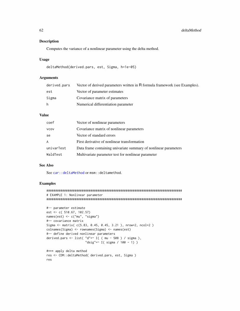
62 deltaMethod

Description

Computes the variance of a nonlinear parameter using the delta method.

Usage

deltaMethod(derived.pars, est, Sigma, h=1e-05)

Arguments

derived.pars Vector of derived parameters written in R formula framework (see Examples).

est Vector of parameter estimates

Sigma Covariance matrix of parameters

h Numerical differentiation parameter

Value

coef Vector of nonlinear parameters

vcov Covariance matrix of nonlinear parameters

se Vector of standard errors

A First derivative of nonlinear transformation

univarTest Data frame containing univariate summary of nonlinear parameters

WaldTest Multivariate parameter test for nonlinear parameter

See Also

See car::deltaMethod or msm::deltamethod.

Examples

############################################################################## EXAMPLE 1: Nonlinear parameter#############################################################################

#-- parameter estimateest <- c( 510.67, 102.57)names(est) <- c("mu", "sigma")#-- covariance matrixSigma <- matrix( c(5.83, 0.45, 0.45, 3.21 ), nrow=2, ncol=2 )colnames(Sigma) <- rownames(Sigma) <- names(est)#-- define derived nonlinear parametersderived.pars <- list( "d"=~ I( ( mu - 508 ) / sigma ),

"dsig"=~ I( sigma / 100 - 1) )

#*** apply delta methodres <- CDM::deltaMethod( derived.pars, est, Sigma )res

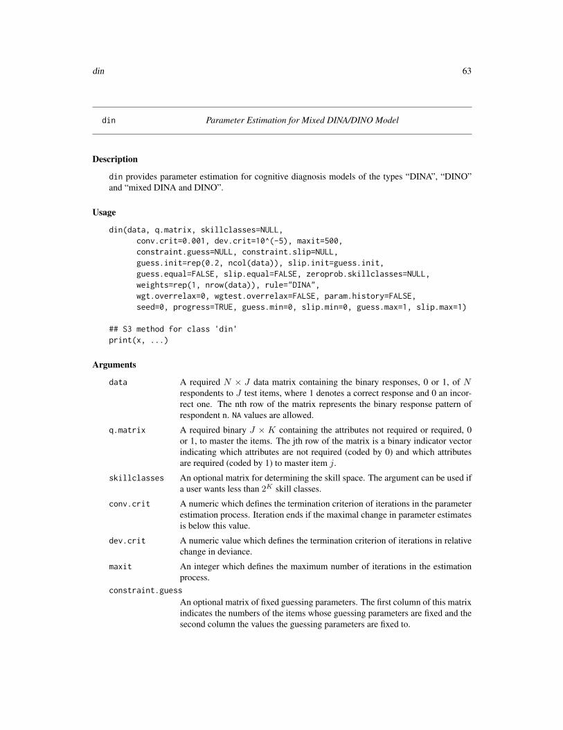
din 63

din Parameter Estimation for Mixed DINA/DINO Model

Description

din provides parameter estimation for cognitive diagnosis models of the types “DINA”, “DINO”and “mixed DINA and DINO”.

Usage

din(data, q.matrix, skillclasses=NULL,conv.crit=0.001, dev.crit=10^(-5), maxit=500,constraint.guess=NULL, constraint.slip=NULL,guess.init=rep(0.2, ncol(data)), slip.init=guess.init,guess.equal=FALSE, slip.equal=FALSE, zeroprob.skillclasses=NULL,weights=rep(1, nrow(data)), rule="DINA",wgt.overrelax=0, wgtest.overrelax=FALSE, param.history=FALSE,seed=0, progress=TRUE, guess.min=0, slip.min=0, guess.max=1, slip.max=1)

## S3 method for class 'din'print(x, ...)

Arguments

data A required N × J data matrix containing the binary responses, 0 or 1, of Nrespondents to J test items, where 1 denotes a correct response and 0 an incor-rect one. The nth row of the matrix represents the binary response pattern ofrespondent n. NA values are allowed.

q.matrix A required binary J × K containing the attributes not required or required, 0or 1, to master the items. The jth row of the matrix is a binary indicator vectorindicating which attributes are not required (coded by 0) and which attributesare required (coded by 1) to master item j.

skillclasses An optional matrix for determining the skill space. The argument can be used ifa user wants less than 2K skill classes.

conv.crit A numeric which defines the termination criterion of iterations in the parameterestimation process. Iteration ends if the maximal change in parameter estimatesis below this value.

dev.crit A numeric value which defines the termination criterion of iterations in relativechange in deviance.

maxit An integer which defines the maximum number of iterations in the estimationprocess.

constraint.guess

An optional matrix of fixed guessing parameters. The first column of this matrixindicates the numbers of the items whose guessing parameters are fixed and thesecond column the values the guessing parameters are fixed to.

64 din

constraint.slip

An optional matrix of fixed slipping parameters. The first column of this matrixindicates the numbers of the items whose slipping parameters are fixed and thesecond column the values the slipping parameters are fixed to.

guess.init An optional initial vector of guessing parameters. Guessing parameters arebounded between 0 and 1.

slip.init An optional initial vector of slipping parameters. Slipping parameters are boundedbetween 0 and 1.

guess.equal An optional logical indicating if all guessing parameters are equal to each other.Default is FALSE.

slip.equal An optional logical indicating if all slipping parameters are equal to each other.Default is FALSE.

zeroprob.skillclasses

An optional vector of integers which indicates which skill classes should havezero probability. Default is NULL (no skill classes with zero probability).

weights An optional vector of weights for the response pattern. Non-integer weightsallow for different sampling schemes.

rule An optional character string or vector of character strings specifying the modelrule that is used. The character strings must be of "DINA" or "DINO". If a vectorof character strings is specified, implying an item wise condensation rule, thevector must be of length J , which is the number of items. The default is thecondensation rule "DINA" for all items.

wgt.overrelax A parameter which is relevant when an overrelaxation algorithm is usedwgtest.overrelax

A logical which indicates if the overrelexation parameter being estimated duringiterations

param.history A logical which indicates if the parameter history during iterations should besaved. The default is FALSE.

seed Simulation seed for initial parameters. A value of zero corresponds to determin-istic starting values, an integer value different from zero to random initial valueswith set.seed(seed).

progress An optional logical indicating whether the function should print the progress ofiteration in the estimation process.

guess.min Minimum value of guessing parameters to be estimated.

slip.min Minimum value of slipping parameters to be estimated.

guess.max Maximum value of guessing parameters to be estimated.

slip.max Maximum value of slipping parameters to be estimated.

x Object of class din


Details

In the CDM DINA (deterministic-input, noisy-and-gate; de la Torre & Douglas, 2004) and DINO(deterministic-input, noisy-or-gate; Templin & Henson, 2006) models endorsement probabilities

din 65

are modeled based on guessing and slipping parameters, given the different skill classes. The prob-ability of respondent n (or corresponding respondents class n) for solving item j is calculated as afunction of the respondent’s latent response ηnj and the guessing and slipping rates gj and sj foritem j conditional on the respondent’s skill class αn:

P (Xnj = 1|αn) = g(1−ηnj)j (1− sj)ηnj .

The respondent’s latent response (class) ηnj is a binary number, 0 or 1, where 1 indicates presenceof all (rule="DINO") or at least one (rule="DINO") required skill(s) for item j, respectively.

DINA and DINO parameter estimation is performed by maximization of the marginal likelihood ofthe data. The a priori distribution of the skill vectors is a uniform distribution. The implementationfollows the EM algorithm by de la Torre (2009).

The function din returns an object of the class din (see ‘Value’), for which plot, print, andsummary methods are provided; plot.din, print.din, and summary.din, respectively.

Value

coef Estimated model parameters. Note that only freely estimated parameters areincluded.

item A data frame giving for each item condensation rule, the estimated guessing andslipping parameters and their standard errors. All entries are rounded to 3 digits.

guess A data frame giving the estimated guessing parameters and their standard errorsfor each item.

slip A data frame giving the estimated slipping parameters and their standard errorsfor each item.

IDI A matrix giving the item discrimination index (IDI; Lee, de la Torre & Park,2012) for each item j

IDIj = 1− sj − gj ,

where a high IDI corresponds to good test items which have both low guessingand slipping rates. Note that a negative IDI indicates violation of the monotonic-ity condition gj < 1− sj . See din for help.

itemfit.rmsea The RMSEA item fit index (see itemfit.rmsea).

mean.rmsea Mean of RMSEA item fit indexes.

loglike A numeric giving the value of the maximized log likelihood.

AIC A numeric giving the AIC value of the model.

BIC A numeric giving the BIC value of the model.

Npars Number of estimated parameters

posterior A matrix given the posterior skill distribution for all respondents. The nth rowof the matrix gives the probabilities for respondent n to possess any of the 2K

skill classes.

like A matrix giving the values of the maximized likelihood for all respondents.

data The input matrix of binary response data.

q.matrix The input matrix of the required attributes.

66 din

pattern A matrix giving the skill classes leading to highest endorsement probability forthe respective response pattern (mle.est) with the corresponding posterior classprobability (mle.post), the attribute classes having the highest occurrence pos-terior probability given the response pattern (map.est) with the correspondingposterior class probability (map.post), and the estimated posterior for each re-sponse pattern (pattern).

attribute.patt A data frame giving the estimated occurrence probabilities of the skill classesand the expected frequency of the attribute classes given the model.

skill.patt A matrix given the population prevalences of the skills.

subj.pattern A vector of strings indicating the item response pattern for each subject.

attribute.patt.splitted

A dataframe giving the skill class of the respondents.

display A character giving the model specified under rule.

item.patt.split

A matrix giving the splitted response pattern.

item.patt.freq A numeric vector given the frequencies of the response pattern in item.patt.split.

seed Used simulation seed for initial parameters

partable Parameter table which is used for coef and vcov.

vcov.derived Design matrix for extended set of parameters in vcov.

converged Logical indicating whether convergence was achieved.

control Optimization parameters used in estimation

Note

The calculation of standard errors using sampling weights which represent multistage samplingschemes is not correct. Please use replication methods (like Jackknife) instead.

References

de la Torre, J. (2009). DINA model parameter estimation: A didactic. Journal of Educational andBehavioral Statistics, 34, 115–130.

de la Torre, J., & Douglas, J. (2004). Higher-order latent trait models for cognitive diagnosis.Psychometrika, 69, 333–353.

Lee, Y.-S., de la Torre, J., & Park, Y. S. (2012). Relationships between cognitive diagnosis, CTT,and IRT indices: An empirical investigation. Asia Pacific Educational Research, 13, 333-345.


Templin, J., & Henson, R. (2006). Measurement of psychological disorders using cognitive diag-nosis models. Psychological Methods, 11, 287–305.

din 67

See Also

plot.din, the S3 method for plotting objects of the class din; print.din, the S3 method forprinting objects of the class din; summary.din, the S3 method for summarizing objects of the classdin, which creates objects of the class summary.din; din, the main function for DINA and DINOparameter estimation, which creates objects of the class din.

See the gdina function for the estimation of the generalized DINA (GDINA) model.

For assessment of model fit see modelfit.cor.din and anova.din.

See itemfit.sx2 for item fit statistics.

See discrim.index for computing discrimination indices.

See also CDM-package for general information about this package.

See the NPCD::JMLE function in the NPCD package for joint maximum likelihood estimation of theDINA, DINO and NIDA model.

See the dina::DINA_Gibbs function in the dina package for MCMC based estimation of the DINAmodel.

Examples

############################################################################## EXAMPLE 1: Examples based on dataset fractions.subtraction.data#############################################################################

## dataset fractions.subtraction.data and corresponding Q-Matrixhead(fraction.subtraction.data)fraction.subtraction.qmatrix

## Misspecification in parameter specification for method CDM::din()## leads to warnings and terminates estimation procedure. E.g.,

# See Q-Matrix specificationfractions.dina.warning1 <- CDM::din(data=fraction.subtraction.data,

q.matrix=t(fraction.subtraction.qmatrix))

# See guess.init specificationfractions.dina.warning2 <- CDM::din(data=fraction.subtraction.data,

q.matrix=fraction.subtraction.qmatrix, guess.init=rep(1.2,ncol(fraction.subtraction.data)))

# See rule specificationfractions.dina.warning3 <- CDM::din(data=fraction.subtraction.data,

q.matrix=fraction.subtraction.qmatrix, rule=c(rep("DINA",10), rep("DINO", 9)))

## Parameter estimation of DINA model# rule="DINA" is defaultfractions.dina <- CDM::din(data=fraction.subtraction.data,

q.matrix=fraction.subtraction.qmatrix, rule="DINA")attributes(fractions.dina)str(fractions.dina)

68 din

## For instance assessing the guessing parameters through## assignmentfractions.dina$guess

## corresponding summaries, including IDI,## most frequent skill classes and information## criteria AIC and BICsummary(fractions.dina)

## In particular, assessing detailed summary through assignmentdetailed.summary.fs <- summary(fractions.dina)str(detailed.summary.fs)

## Item discrimination index of item 8 is too low. This is also## visualized in the first plotplot(fractions.dina)

## The reason therefore is a high guessing parameterround(fractions.dina$guess[,1], 2)

## Estimate DINA model with different random initial parameters using seed=1345fractions.dina1 <- CDM::din(data=fraction.subtraction.data,

q.matrix=fraction.subtraction.qmatrix, rule="DINA", seed=1345)

## Fix the guessing parameters of items 5, 8 and 9 equal to .20# define a constraint.guess matrixconstraint.guess <- matrix(c(5,8,9, rep(0.2, 3)), ncol=2)fractions.dina.fixed <- CDM::din(data=fraction.subtraction.data,

q.matrix=fraction.subtraction.qmatrix,constraint.guess=constraint.guess)

## The second plot shows the expected (MAP) and observed skill## probabilities. The third plot visualizes the skill class## occurrence probabilities; Only the 'top.n.skill.classes' most frequent## skill classes are labeled; it is obvious that the skill class '11111111'## (all skills are mastered) is the most probable in this population.## The fourth plot shows the skill probabilities conditional on response## patterns; in this population the skills 3 and 6 seem to be## mastered easier than the others. The fourth plot shows the## skill probabilities conditional on a specified response## pattern; it is shown whether a skill is mastered (above## .5+'uncertainty') unclassifiable (within the boundaries) or## not mastered (below .5-'uncertainty'). In this case, the## 527th respondent was chosen; if no response pattern is## specified, the plot will not be shown (of course)pattern <- paste(fraction.subtraction.data[527, ], collapse="")plot(fractions.dina, pattern=pattern, display.nr=4)

#uncertainty=0.1, top.n.skill.classes=6 are defaultplot(fractions.dina.fixed, uncertainty=0.1, top.n.skill.classes=6,

pattern=pattern)

## Not run:

din 69

############################################################################## EXAMPLE 2: Examples based on dataset sim.dina#############################################################################

# DINA Modeld1 <- CDM::din(sim.dina, q.matr=sim.qmatrix, rule="DINA",

conv.crit=0.01, maxit=500, progress=TRUE)summary(d1)

# DINA model with hierarchical skill classes (Hierarchical DINA model)# 1st step: estimate an initial full model to look at the indexing# of skill classesd0 <- CDM::din(sim.dina, q.matr=sim.qmatrix, maxit=1)d0$attribute.patt.splitted# [,1] [,2] [,3]# [1,] 0 0 0# [2,] 1 0 0# [3,] 0 1 0# [4,] 0 0 1# [5,] 1 1 0# [6,] 1 0 1# [7,] 0 1 1# [8,] 1 1 1## In this example, following hierarchical skill classes are only allowed:# 000, 001, 011, 111# We define therefore a vector of indices for skill classes with# zero probabilities (see entries in the rows of the matrix# d0$attribute.patt.splitted above)zeroprob.skillclasses <- c(2,3,5,6) # classes 100, 010, 110, 101# estimate the hierarchical DINA modeld1a <- CDM::din(sim.dina, q.matr=sim.qmatrix,

zeroprob.skillclasses=zeroprob.skillclasses )summary(d1a)

# Mixed DINA and DINO Modeld1b <- CDM::din(sim.dina, q.matr=sim.qmatrix, rule=

c(rep("DINA", 7), rep("DINO", 2)), conv.crit=0.01,maxit=500, progress=FALSE)

summary(d1b)

# DINO Modeld2 <- CDM::din(sim.dina, q.matr=sim.qmatrix, rule="DINO",

conv.crit=0.01, maxit=500, progress=FALSE)summary(d2)

# Comparison of DINA and DINO estimateslapply(list("guessing"=rbind("DINA"=d1$guess[,1],

"DINO"=d2$guess[,1]), "slipping"=rbind("DINA"=d1$slip[,1], "DINO"=d2$slip[,1])), round, 2)

# Comparison of the information criteriac("DINA"=d1$AIC, "MIXED"=d1b$AIC, "DINO"=d2$AIC)

70 din

# following estimates:d1$coef # guessing and slipping parameterd1$guess # guessing parameterd1$slip # slipping parameterd1$skill.patt # probabilities for skillsd1$attribute.patt # skill classes with probabilitiesd1$subj.pattern # pattern per subject

# posterior probabilities for every response patternd1$posterior

# Equal guessing parametersd2a <- CDM::din( data=sim.dina, q.matrix=sim.qmatrix,

guess.equal=TRUE, slip.equal=FALSE )d2a$coef

# Equal guessing and slipping parametersd2b <- CDM::din( data=sim.dina, q.matrix=sim.qmatrix,

guess.equal=TRUE, slip.equal=TRUE )d2b$coef

############################################################################## EXAMPLE 3: Examples based on dataset sim.dino#############################################################################

# DINO Estimationd3 <- CDM::din(sim.dino, q.matr=sim.qmatrix, rule="DINO",

conv.crit=0.005, progress=FALSE)

# Mixed DINA and DINO Modeld3b <- CDM::din(sim.dino, q.matr=sim.qmatrix,

rule=c(rep("DINA", 4), rep("DINO", 5)), conv.crit=0.001,progress=FALSE)

# DINA Estimationd4 <- CDM::din(sim.dino, q.matr=sim.qmatrix, rule="DINA",

conv.crit=0.005, progress=FALSE)

# Comparison of DINA and DINO estimateslapply(list("guessing"=rbind("DINO"=d3$guess[,1], "DINA"=d4$guess[,1]),

"slipping"=rbind("DINO"=d3$slip[,1], "DINA"=d4$slip[,1])), round, 2)

# Comparison of the information criteriac("DINO"=d3$AIC, "MIXED"=d3b$AIC, "DINA"=d4$AIC)

############################################################################## EXAMPLE 4: Example estimation with weights based on dataset sim.dina#############################################################################

# Here, a weighted maximum likelihood estimation is used# This could be useful for survey data.

din 71

# i.e. first 200 persons have weight 2, the other have weight 1(weights <- c(rep(2, 200), rep(1, 200)))

d5 <- CDM::din(sim.dina, sim.qmatrix, rule="DINA", conv.crit=0.005, weights=weights, progress=FALSE)

# Comparison of the information criteriac("DINA"=d1$AIC, "WEIGHTS"=d5$AIC)

############################################################################## EXAMPLE 5: Example estimation within a balanced incomplete## block (BIB) design generated on dataset sim.dina#############################################################################

# generate BIB data

# The next example shows that the din function works for# (relatively arbitrary) missing value pattern

# Here, a missing by design is generated in the dataset dinadat.bibsim.dina.bib <- sim.dinasim.dina.bib[1:100, 1:3] <- NAsim.dina.bib[101:300, 4:8] <- NAsim.dina.bib[301:400, c(1,2,9)] <- NA

d6 <- CDM::din(sim.dina.bib, sim.qmatrix, rule="DINA",conv.crit=0.0005, weights=weights, maxit=200)

d7 <- CDM::din(sim.dina.bib, sim.qmatrix, rule="DINO",conv.crit=0.005, weights=weights)

# Comparison of DINA and DINO estimateslapply(list("guessing"=rbind("DINA"=d6$guess[,1],

"DINO"=d7$guess[,1]), "slipping"=rbind("DINA"=d6$slip[,1], "DINO"=d7$slip[,1])), round, 2)

############################################################################## EXAMPLE 6: DINA model with attribute hierarchy#############################################################################

set.seed(987)# assumed skill distribution: P(000)=P(100)=P(110)=P(111)=.245 and# "deviant pattern": P(010)=.02K <- 3 # number of skills

# define alphaalpha <- scan()

0 0 01 0 01 1 01 1 10 1 0

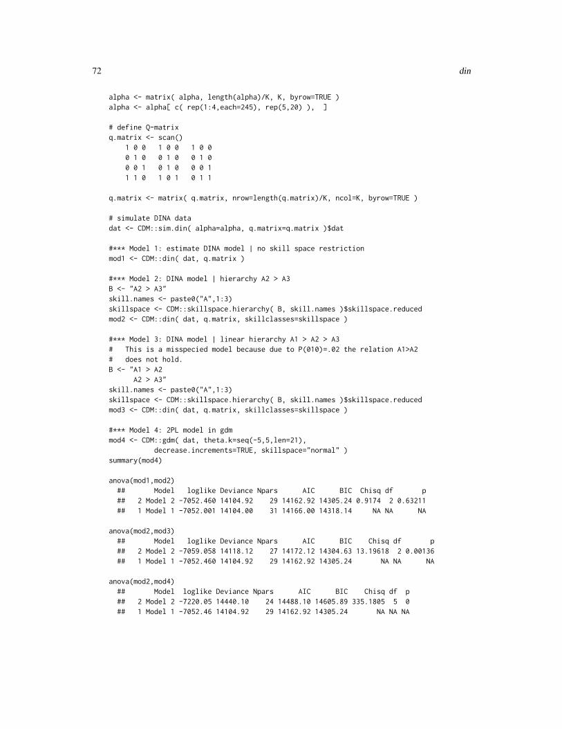
72 din

alpha <- matrix( alpha, length(alpha)/K, K, byrow=TRUE )alpha <- alpha[ c( rep(1:4,each=245), rep(5,20) ), ]

# define Q-matrixq.matrix <- scan()

1 0 0 1 0 0 1 0 00 1 0 0 1 0 0 1 00 0 1 0 1 0 0 0 11 1 0 1 0 1 0 1 1

q.matrix <- matrix( q.matrix, nrow=length(q.matrix)/K, ncol=K, byrow=TRUE )

# simulate DINA datadat <- CDM::sim.din( alpha=alpha, q.matrix=q.matrix )$dat

#*** Model 1: estimate DINA model | no skill space restrictionmod1 <- CDM::din( dat, q.matrix )

#*** Model 2: DINA model | hierarchy A2 > A3B <- "A2 > A3"skill.names <- paste0("A",1:3)skillspace <- CDM::skillspace.hierarchy( B, skill.names )$skillspace.reducedmod2 <- CDM::din( dat, q.matrix, skillclasses=skillspace )

#*** Model 3: DINA model | linear hierarchy A1 > A2 > A3# This is a misspecied model because due to P(010)=.02 the relation A1>A2# does not hold.B <- "A1 > A2

A2 > A3"skill.names <- paste0("A",1:3)skillspace <- CDM::skillspace.hierarchy( B, skill.names )$skillspace.reducedmod3 <- CDM::din( dat, q.matrix, skillclasses=skillspace )

#*** Model 4: 2PL model in gdmmod4 <- CDM::gdm( dat, theta.k=seq(-5,5,len=21),

decrease.increments=TRUE, skillspace="normal" )summary(mod4)

anova(mod1,mod2)## Model loglike Deviance Npars AIC BIC Chisq df p## 2 Model 2 -7052.460 14104.92 29 14162.92 14305.24 0.9174 2 0.63211## 1 Model 1 -7052.001 14104.00 31 14166.00 14318.14 NA NA NA

anova(mod2,mod3)## Model loglike Deviance Npars AIC BIC Chisq df p## 2 Model 2 -7059.058 14118.12 27 14172.12 14304.63 13.19618 2 0.00136## 1 Model 1 -7052.460 14104.92 29 14162.92 14305.24 NA NA NA


din 73

# compare fit statisticssummary( CDM::modelfit.cor.din( mod2 ) )summary( CDM::modelfit.cor.din( mod4 ) )

############################################################################## EXAMPLE 7: Fitting the basic local independence model (BLIM) with din#############################################################################

library(pks)data(DoignonFalmagne7, package="pks")

## str(DoignonFalmagne7)## $ K : int [1:9, 1:5] 0 1 0 1 1 1 1 1 1 0 ...## ..- attr(*, "dimnames")=List of 2## .. ..$ : chr [1:9] "00000" "10000" "01000" "11000" ...## .. ..$ : chr [1:5] "a" "b" "c" "d" ...## $ N.R: Named int [1:32] 80 92 89 3 2 1 89 16 18 10 ...## ..- attr(*, "names")=chr [1:32] "00000" "10000" "01000" "00100" ...

# The idea is to fit the local independence model with the din function.# This can be accomplished by specifying a DINO model with# prespecified skill classes.

# extract datasetdat <- as.numeric( unlist( sapply( names(DoignonFalmagne7$N.R),

FUN=function( ll){ strsplit( ll, split="") } ) ) )dat <- matrix( dat, ncol=5, byrow=TRUE )colnames(dat) <- colnames(DoignonFalmagne7$K)rownames(dat) <- names(DoignonFalmagne7$N.R)

# sample weightsweights <- DoignonFalmagne7$N.R

# define Q-matrixq.matrix <- t(DoignonFalmagne7$K)v1 <- colnames(q.matrix) <- paste0("S", colnames(q.matrix))q.matrix <- q.matrix[, - 1] # remove S00000

# define skill classesSC <- ncol(q.matrix)skillclasses <- matrix( 0, nrow=SC+1, ncol=SC)colnames(skillclasses) <- colnames(q.matrix)rownames(skillclasses) <- v1skillclasses[ cbind( 2:(SC+1), 1:SC ) ] <- 1

# estimate BLIM with din functionmod1 <- CDM::din(data=dat, q.matrix=q.matrix, skillclasses=skillclasses,

rule="DINO", weights=weights )summary(mod1)

## Item parameters## item guess slip IDI rmsea## a a 0.158 0.162 0.680 0.011## b b 0.145 0.159 0.696 0.009## c c 0.008 0.181 0.811 0.001

74 din.deterministic

## d d 0.012 0.129 0.859 0.001## e e 0.025 0.146 0.828 0.007

# estimate basic local independence model with pks packagemod2 <- pks::blim(K, N.R, method="ML") # maximum likelihood estimation by EM algorithmmod2

## Error and guessing parameters## beta eta## a 0.164871 0.103065## b 0.163113 0.095074## c 0.188839 0.000004## d 0.079835 0.000003## e 0.088648 0.019910

## End(Not run)

din.deterministic Deterministic Classification and Joint Maximum Likelihood Estima-tion of the Mixed DINA/DINO Model

Description

This function allows the estimation of the mixed DINA/DINO model by joint maximum likelihoodand a deterministic classification based on ideal latent responses.

Usage

din.deterministic(dat, q.matrix, rule="DINA", method="JML", conv=0.001,maxiter=300, increment.factor=1.05, progress=TRUE)

Arguments

dat Data frame of dichotomous item responsesq.matrix Q-matrix with binary entries (see din).rule The condensation rule (see din).method Estimation method. The default is joint maximum likelihood estimation (JML).

Other options include an adaptive estimation of guessing and slipping param-eters (adaptive) while using these estimated parameters as weights in the in-dividual deviation function and classification based on the Hamming distance(hamming) and the weighted Hamming distance (weighted.hamming) (see Chiu& Douglas, 2013).

conv Convergence criterion for guessing and slipping parametersmaxiter Maximum number of iterationsincrement.factor

A numeric value of at least one which could help to improve convergence be-havior and decreases parameter increments in every iteration. This option isdisabled by setting this argument to 1.


din.deterministic 75

Value


attr.est Estimated attribute patterns

criterion Criterion of the classification function. For joint maximum likelihood it is thedeviance.

guess Estimated guessing parameters

slip Estimated slipping parameters

prederror Average individual prediction error

q.matrix Used Q-matrix

dat Used data frame

References

Chiu, C. Y., & Douglas, J. (2013). A nonparametric approach to cognitive diagnosis by proximityto ideal response patterns. Journal of Classification, 30, 225-250.

See Also

For estimating the mixed DINA/DINO model using marginal maximum likelihood estimation seedin.

See also the NPCD::JMLE function in the NPCD package for joint maximum likelihood estimationof the DINA or the DINO model.

Examples

############################################################################## EXAMPLE 1: 13 items and 3 attributes#############################################################################

set.seed(679)N <- 3000# specify true Q-matrixq.matrix <- matrix( 0, 13, 3 )q.matrix[1:3,1] <- 1q.matrix[4:6,2] <- 1q.matrix[7:9,3] <- 1q.matrix[10,] <- c(1,1,0)q.matrix[11,] <- c(1,0,1)q.matrix[12,] <- c(0,1,1)q.matrix[13,] <- c(1,1,1)q.matrix <- rbind( q.matrix, q.matrix )colnames(q.matrix) <- paste0("Attr",1:ncol(q.matrix))

# simulate data according to the DINA modeldat <- CDM::sim.din( N=N, q.matrix)$dat

# Joint maximum likelihood estimation (the default: method="JML")res1 <- CDM::din.deterministic( dat, q.matrix )

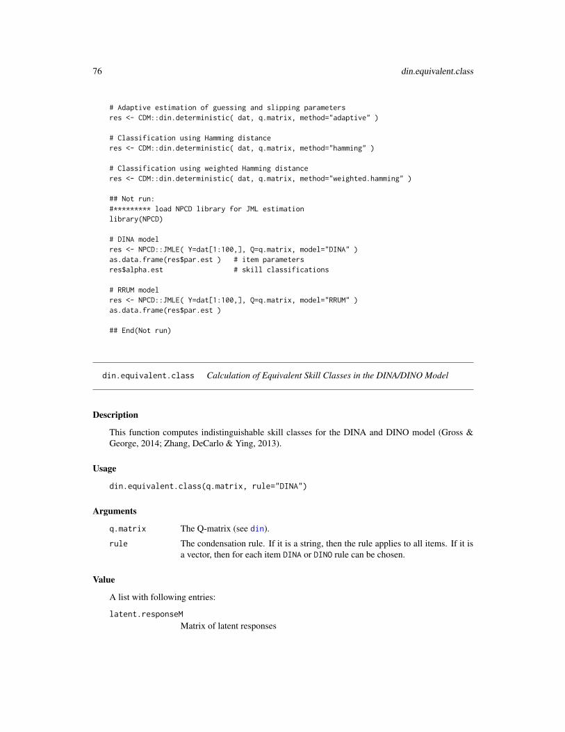
76 din.equivalent.class

# Adaptive estimation of guessing and slipping parametersres <- CDM::din.deterministic( dat, q.matrix, method="adaptive" )

# Classification using Hamming distanceres <- CDM::din.deterministic( dat, q.matrix, method="hamming" )

# Classification using weighted Hamming distanceres <- CDM::din.deterministic( dat, q.matrix, method="weighted.hamming" )

## Not run:#********* load NPCD library for JML estimationlibrary(NPCD)

# DINA modelres <- NPCD::JMLE( Y=dat[1:100,], Q=q.matrix, model="DINA" )as.data.frame(res$par.est ) # item parametersres$alpha.est # skill classifications

# RRUM modelres <- NPCD::JMLE( Y=dat[1:100,], Q=q.matrix, model="RRUM" )as.data.frame(res$par.est )

## End(Not run)

din.equivalent.class Calculation of Equivalent Skill Classes in the DINA/DINO Model

Description

This function computes indistinguishable skill classes for the DINA and DINO model (Gross &George, 2014; Zhang, DeCarlo & Ying, 2013).

Usage

din.equivalent.class(q.matrix, rule="DINA")

Arguments

q.matrix The Q-matrix (see din).

rule The condensation rule. If it is a string, then the rule applies to all items. If it isa vector, then for each item DINA or DINO rule can be chosen.

Value

A list with following entries:

latent.responseM

Matrix of latent responses

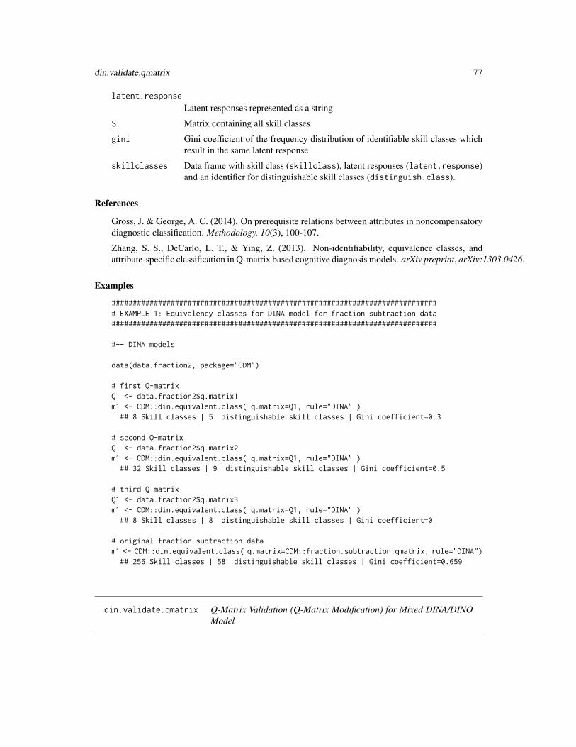
din.validate.qmatrix 77

latent.response

Latent responses represented as a string

S Matrix containing all skill classes

gini Gini coefficient of the frequency distribution of identifiable skill classes whichresult in the same latent response

skillclasses Data frame with skill class (skillclass), latent responses (latent.response)and an identifier for distinguishable skill classes (distinguish.class).

References

Gross, J. & George, A. C. (2014). On prerequisite relations between attributes in noncompensatorydiagnostic classification. Methodology, 10(3), 100-107.

Zhang, S. S., DeCarlo, L. T., & Ying, Z. (2013). Non-identifiability, equivalence classes, andattribute-specific classification in Q-matrix based cognitive diagnosis models. arXiv preprint, arXiv:1303.0426.

Examples

############################################################################## EXAMPLE 1: Equivalency classes for DINA model for fraction subtraction data#############################################################################

#-- DINA models

data(data.fraction2, package="CDM")

# first Q-matrixQ1 <- data.fraction2$q.matrix1m1 <- CDM::din.equivalent.class( q.matrix=Q1, rule="DINA" )

## 8 Skill classes | 5 distinguishable skill classes | Gini coefficient=0.3

# second Q-matrixQ1 <- data.fraction2$q.matrix2m1 <- CDM::din.equivalent.class( q.matrix=Q1, rule="DINA" )


# third Q-matrixQ1 <- data.fraction2$q.matrix3m1 <- CDM::din.equivalent.class( q.matrix=Q1, rule="DINA" )

## 8 Skill classes | 8 distinguishable skill classes | Gini coefficient=0

# original fraction subtraction datam1 <- CDM::din.equivalent.class( q.matrix=CDM::fraction.subtraction.qmatrix, rule="DINA")


din.validate.qmatrix Q-Matrix Validation (Q-Matrix Modification) for Mixed DINA/DINOModel

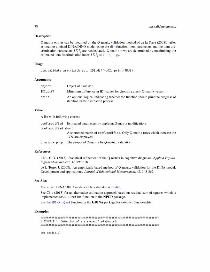
78 din.validate.qmatrix

Description

Q-matrix entries can be modified by the Q-matrix validation method of de la Torre (2008). Afterestimating a mixed DINA/DINO model using the din function, item parameters and the item dis-crimination parameters IDIj are recalculated. Q-matrix rows are determined by maximizing theestimated item discrimination index IDIj = 1− sj − gj .

Usage

din.validate.qmatrix(object, IDI_diff=.02, print=TRUE)

Arguments

object Object of class din

IDI_diff Minimum difference in IDI values for choosing a new Q-matrix vector

print An optional logical indicating whether the function should print the progress ofiteration in the estimation process.

Value


coef.modified Estimated parameters by applying Q-matrix modificationscoef.modified.short

A shortened matrix of coef.modified. Only Q-matrix rows which increase theIDI are displayed.

q.matrix.prop The proposed Q-matrix by Q-matrix validation.

References

Chiu, C. Y. (2013). Statistical refinement of the Q-matrix in cognitive diagnosis. Applied Psycho-logical Measurement, 37, 598-618.

de la Torre, J. (2008). An empirically based method of Q-matrix validation for the DINA model:Development and applications. Journal of Educational Measurement, 45, 343-362.

See Also

The mixed DINA/DINO model can be estimated with din.

See Chiu (2013) for an alternative estimation approach based on residual sum of squares which isimplemented NPCD::Qrefine function in the NPCD package.

See the GDINA::Qval function in the GDINA package for extended functionality.

Examples

############################################################################## EXAMPLE 1: Detection of a mis-specified Q-matrix#############################################################################

set.seed(679)

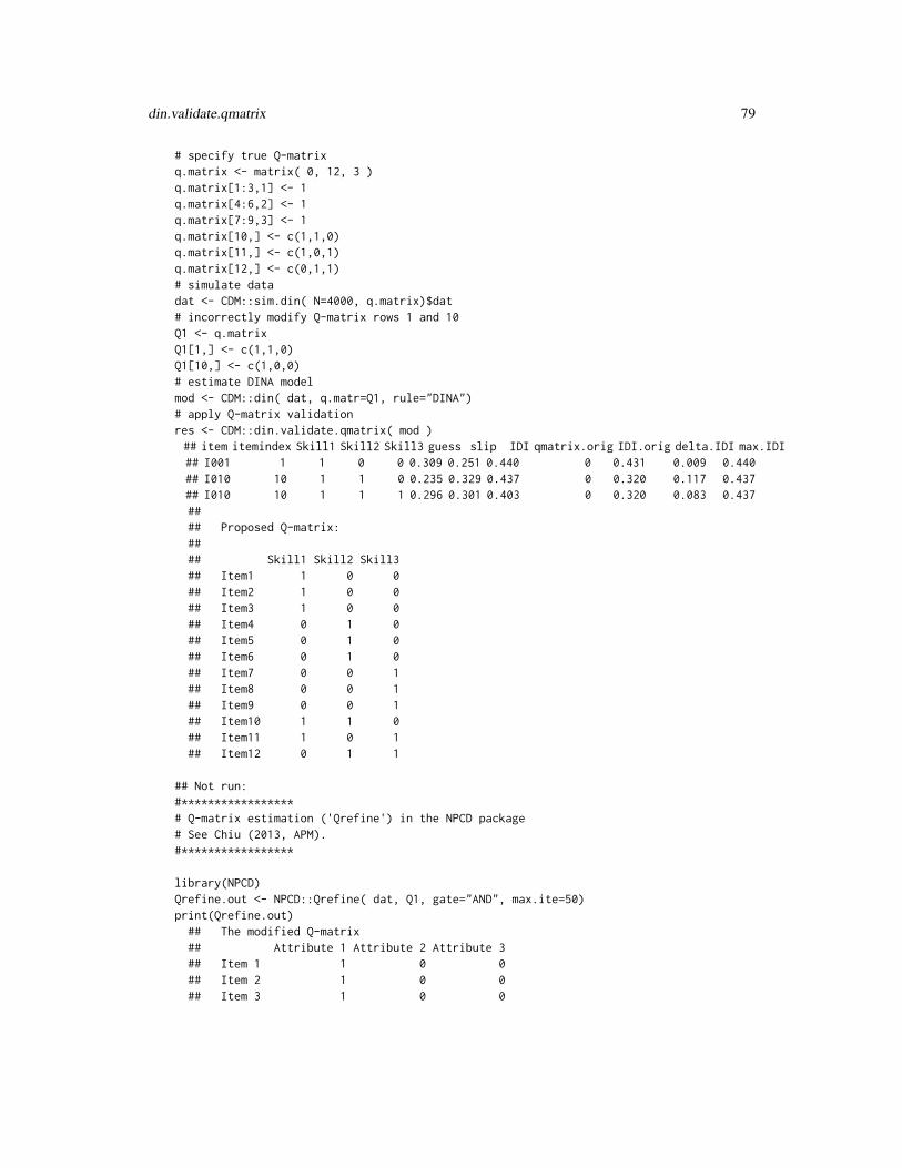
din.validate.qmatrix 79

# specify true Q-matrixq.matrix <- matrix( 0, 12, 3 )q.matrix[1:3,1] <- 1q.matrix[4:6,2] <- 1q.matrix[7:9,3] <- 1q.matrix[10,] <- c(1,1,0)q.matrix[11,] <- c(1,0,1)q.matrix[12,] <- c(0,1,1)# simulate datadat <- CDM::sim.din( N=4000, q.matrix)$dat# incorrectly modify Q-matrix rows 1 and 10Q1 <- q.matrixQ1[1,] <- c(1,1,0)Q1[10,] <- c(1,0,0)# estimate DINA modelmod <- CDM::din( dat, q.matr=Q1, rule="DINA")# apply Q-matrix validationres <- CDM::din.validate.qmatrix( mod )## item itemindex Skill1 Skill2 Skill3 guess slip IDI qmatrix.orig IDI.orig delta.IDI max.IDI## I001 1 1 0 0 0.309 0.251 0.440 0 0.431 0.009 0.440## I010 10 1 1 0 0.235 0.329 0.437 0 0.320 0.117 0.437## I010 10 1 1 1 0.296 0.301 0.403 0 0.320 0.083 0.437#### Proposed Q-matrix:#### Skill1 Skill2 Skill3## Item1 1 0 0## Item2 1 0 0## Item3 1 0 0## Item4 0 1 0## Item5 0 1 0## Item6 0 1 0## Item7 0 0 1## Item8 0 0 1## Item9 0 0 1## Item10 1 1 0## Item11 1 0 1## Item12 0 1 1

## Not run:#*****************# Q-matrix estimation ('Qrefine') in the NPCD package# See Chiu (2013, APM).#*****************

library(NPCD)Qrefine.out <- NPCD::Qrefine( dat, Q1, gate="AND", max.ite=50)print(Qrefine.out)

## The modified Q-matrix## Attribute 1 Attribute 2 Attribute 3## Item 1 1 0 0## Item 2 1 0 0## Item 3 1 0 0

80 din_identifiability

## Item 4 0 1 0## Item 5 0 1 0## Item 6 0 1 0## Item 7 0 0 1## Item 8 0 0 1## Item 9 0 0 1## Item 10 1 1 0## Item 11 1 0 1## Item 12 0 1 1#### The modified entries## Item Attribute## [1,] 1 2## [2,] 10 2

plot(Qrefine.out)

## End(Not run)

din_identifiability Identifiability Conditions of the DINA Model

Description

Check necessary and sufficient identifiability conditions of the DINA model according Gu and Xu(xxxx) for a given Q-matrix.

Usage

din_identifiability(q.matrix)

## S3 method for class 'din_identifiability'summary(object, ...)

Arguments

q.matrix Q-matrix

object Object of class din_identifiability


Value

List with values

dina_identified

Logical indicating whether the DINA model is identified

index_single Condition 1: vector of logicals indicating whether skills are measured by at leastone item with a single loading

discrim.index 81

is_three_items Condition 2: vector of logicals indicating whether skills are measured by at leastthree items

submat_distinct

Condition 3: logical indicating whether all columns of the submatrix Q∗ aredistinct.

References

Gu, Y., & Xu, G. (2018). The sufficient and necessary condition for the identifiability and estima-bility of the DINA model. Psychometrika, xx(xx), xxx-xxx. https://doi.org/10.1007/s11336-018-9619-8

See Also

See din.equivalent.class for equivalent (i.e., non-distinguishable) skill classes in the DINAmodel.

Examples

############################################################################## EXAMPLE 1: Some examples of Gu and Xu (2019)#############################################################################

#* Matrix 1 in Equation (5) of Gu & Xu (2019)Q1 <- diag(3)Q2 <- matrix( scan(text="1 1 0 1 0 1 1 1 1 1 1 1"), ncol=3, byrow=TRUE)Q <- rbind(Q1, Q2)

res <- CDM::din_identifiability(q.matrix=Q)summary(res)

# remove two itemsres <- CDM::din_identifiability(q.matrix=Q[-c(2,5),])summary(res)

#* Matrix 1 in Equation (6) of Gu & Xu (2019)Q1 <- diag(3)Q2 <- matrix( c(1,1,1), nrow=4, ncol=3, byrow=TRUE)Q <- rbind(Q1, Q2)

res <- CDM::din_identifiability(q.matrix=Q)summary(res)

discrim.index Discrimination Indices at Item-Attribute, Item and Test Level

Description

Computes discrimination indices at the probability metric (de la Torre, 2008; Henson, DiBello &Stout, 2018).

82 discrim.index

Usage

discrim.index(object, ...)

## S3 method for class 'din'discrim.index(object, ...)

## S3 method for class 'gdina'discrim.index(object, ...)

## S3 method for class 'mcdina'discrim.index(object, ...)

## S3 method for class 'discrim.index'summary(object, file=NULL, digits=3, ...)

Arguments

object Object of class din or gdina.

file Optional file name for a file in which the summary output should be sunk

digits Number of digits for rounding


Details

If item j possessesHj categories, the item-attribute specific discrimination for attribute k accordingto Henson et al. (2018) is defined as

DIjk =1

2maxα

Hj∑h=1

|P (Xj = h|α)− P (Xj = h|α(−k))|

whereα(−k) andα differ only in attribute k. The indexDIjk can be found as the value discrim_item_attribute.The test-level discrimination index is defined as

DI =1

J

J∑j=1

maxk

DIjk

and can be found in discrim_test.

According to de la Torre (2008) and de la Torre, Rossi and van der Ark (2018), the item discrimi-nation index (IDI) is defined as

IDIj = maxα1,α2,h

|P (Xj = h|α1)− P (Xj = h|α2)|

and can be found as idi in the values list.

discrim.index 83

Value


discrim_item_attribute

Discrimination indices DIjk at item level for each attribute

idi Item discrimination index IDIjdiscrim_test Discrimination index at test level

References

de la Torre, J. (2008). An empirically based method of Q-matrix validation for the DINA model:Development and applications. Journal of Educational Measurement, 45, 343-362.http://dx.doi.org/10.1111/j.1745-3984.2008.00069.x

de la Torre, J., van der Ark, L. A., & Rossi, G. (2018). Analysis of clinical data from a cognitivediagnosis modeling framework. Measurement and Evaluation in Counseling and Development,51(4), 281-296. https://doi.org/10.1080/07481756.2017.1327286

Henson, R., DiBello, L., & Stout, B. (2018). A generalized approach to defining item discriminationfor DCMs. Measurement: Interdisciplinary Research and Perspectives, 16(1), 18-29.http://dx.doi.org/10.1080/15366367.2018.1436855

See Also

See cdi.kli for discrimination indices based on the Kullback-Leibler information.

For a fitted model mod in the GDINA package, discrimination indices can be extracted by themethod extract(mod,"discrim") (GDINA::extract).

Examples

## Not run:############################################################################## EXAMPLE 1: DINA and GDINA model#############################################################################


#-- fit GDINA and DINA modelmod1 <- CDM::gdina( sim.dina, q.matrix=sim.qmatrix )mod2 <- CDM::din( sim.dina, q.matrix=sim.qmatrix )

#-- compute discrimination indicesdimod1 <- CDM::discrim.index(mod1)dimod2 <- CDM::discrim.index(mod2)summary(dimod1)summary(dimod2)

## End(Not run)

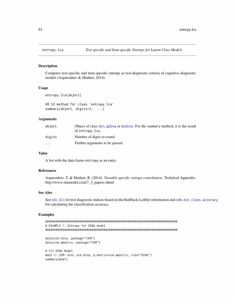
84 entropy.lca

entropy.lca Test-specific and Item-specific Entropy for Latent Class Models

Description

Computes test-specific and item-specific entropy as test-diagnostic criteria of cognitive diagnosticmodels (Asparouhov & Muthen, 2014).

Usage

entropy.lca(object)

## S3 method for class 'entropy.lca'summary(object, digits=2, ...)

Arguments

object Object of class din, gdina or mcdina. For the summary method, it is the resultof entropy.lca.

digits Number of digits to round


Value

A list with the data frame entropy as an entry.

References

Asparouhov, T. & Muthen, B. (2014). Variable-specific entropy contribution. Technical Appendix.http://www.statmodel.com/7_3_papers.shtml

See Also

See cdi.kli for test diagnostic indices based on the Kullback-Leibler information and cdm.est.class.accuracyfor calculating the classification accuracy.

Examples

############################################################################## EXAMPLE 1: Entropy for DINA model#############################################################################


# fit DINA Modelmod1 <- CDM::din( sim.dina, q.matrix=sim.qmatrix, rule="DINA")summary(mod1)

equivalent.dina 85

# compute entropy for test and itemsemod1 <- CDM::entropy.lca( mod1 )summary(emod1)

## Not run:############################################################################## EXAMPLE 2: Entropy for polytomous GDINA model#############################################################################

data(data.pgdina, package="CDM")

dat <- data.pgdina$datq.matrix <- data.pgdina$q.matrix

# pGDINA model with "DINA rule"mod1 <- CDM::gdina( dat, q.matrix=q.matrix, rule="DINA")summary(mod1)

# compute entropyemod1 <- CDM::entropy.lca( mod1 )summary(emod1)

############################################################################## EXAMPLE 3: Entropy for MCDINA model#############################################################################

data(data.cdm02, package="CDM")

dat <- data.cdm02$dataq.matrix <- data.cdm02$q.matrix

# estimate model with polytomous atributemod1 <- CDM::mcdina( dat, q.matrix=q.matrix )summary(mod1)# computre entropyemod1 <- CDM::entropy.lca( mod1 )summary(emod1)

## End(Not run)

equivalent.dina Determination of a Statistically Equivalent DINA Model

Description

This function determines a statistically equivalent DINA model given a Q-matrix using the methodof von Davier (2014). Thereby, the dimension of the skill space is expanded, but in the reparam-eterized version, the Q-matrix has a simple structure or the IRT model is no longer be conjuctive(like in DINA) due to a redefinition of the skill space.

86 equivalent.dina

Usage

equivalent.dina(q.matrix, reparameterization="B")

Arguments

q.matrix The Q-matrix (see din)reparameterization

The used reparameterization (see von Davier, 2014). A and B are possible repa-rameterizations.

Value


q.matrix Original Q-matrix

q.matrix.ast Reparameterized Q-matrix

alpha Original skill space

alpha.ast Reparameterized skill space

References

von Davier, M. (2014). The DINA model as a constrained general diagnostic model: Two variantsof a model equivalency. British Journal of Mathematical and Statistical Psychology, 67, 49-71.

Examples

############################################################################## EXAMPLE 1: Toy example#############################################################################

# define a Q-matrixQ <- matrix( c( 1,0,0, 0,1,0,

0,0,1, 1,0,1, 1,1,1 ), byrow=TRUE, ncol=3 )Q <- Q[ rep(1:(nrow(Q)),each=2), ]

# equivalent DINA model (using the default reparameterization B)res1 <- CDM::equivalent.dina( q.matrix=Q )res1

# equivalent DINA model (reparametrization A)res2 <- CDM::equivalent.dina( q.matrix=Q, reparameterization="A")res2

## Not run:############################################################################## EXAMPLE 2: Estimation with two equivalent DINA models#############################################################################

# simulate dataset.seed(789)

eval_likelihood 87

D <- ncol(Q)mean.alpha <- c( -.5, .5, 0 )r1 <- .5Sigma.alpha <- matrix( r1, D, D ) + diag(1-r1,D)dat1 <- CDM::sim.din( N=2000, q.matrix=Q, mean=mean.alpha, Sigma=Sigma.alpha )

# estimate DINA modelmod1 <- CDM::din( dat1$dat, q.matrix=Q )

# estimate equivalent DINA modelmod2 <- CDM::din( dat1$dat, q.matrix=res1$q.matrix.ast, skillclasses=res1$alpha.ast)# restricted skill space must be defined by using the argument 'skillclasses'

# compare model summariessummary(mod2)summary(mod1)

# compare estimated item parameterscbind( mod2$coef, mod1$coef )

# compare estimated skill class probabilitiesround( cbind( mod2$attribute.patt, mod1$attribute.patt ), 4 )

############################################################################## EXAMPLE 3: Examples from von Davier (2014)#############################################################################

# define Q-matrixQ <- matrix( 0, nrow=8, ncol=3 )Q[2, ] <- c(1,0,0)Q[3, ] <- c(0,1,0)Q[4, ] <- c(1,1,0)Q[5, ] <- c(0,0,1)# Q[6, ] <- c(1,0,1)Q[6, ] <- c(0,0,1)Q[7, ] <- c(0,1,1)Q[8, ] <- c(1,1,1)

#- parametrization Ares1 <- CDM::equivalent.dina(q.matrix=Q, reparameterization="A")res1

#- parametrization Bres2 <- CDM::equivalent.dina(q.matrix=Q, reparameterization="B")res2

## End(Not run)

eval_likelihood Evaluation of Likelihood

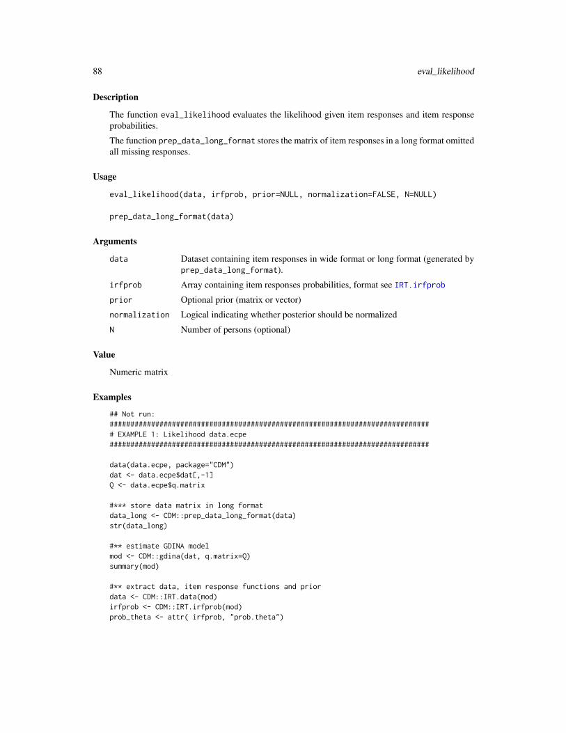
88 eval_likelihood

Description

The function eval_likelihood evaluates the likelihood given item responses and item responseprobabilities.

The function prep_data_long_format stores the matrix of item responses in a long format omittedall missing responses.

Usage

eval_likelihood(data, irfprob, prior=NULL, normalization=FALSE, N=NULL)

prep_data_long_format(data)

Arguments

data Dataset containing item responses in wide format or long format (generated byprep_data_long_format).

irfprob Array containing item responses probabilities, format see IRT.irfprob

prior Optional prior (matrix or vector)

normalization Logical indicating whether posterior should be normalized

N Number of persons (optional)

Value

Numeric matrix

Examples

## Not run:############################################################################## EXAMPLE 1: Likelihood data.ecpe#############################################################################

data(data.ecpe, package="CDM")dat <- data.ecpe$dat[,-1]Q <- data.ecpe$q.matrix

#*** store data matrix in long formatdata_long <- CDM::prep_data_long_format(data)str(data_long)

#** estimate GDINA modelmod <- CDM::gdina(dat, q.matrix=Q)summary(mod)

#** extract data, item response functions and priordata <- CDM::IRT.data(mod)irfprob <- CDM::IRT.irfprob(mod)prob_theta <- attr( irfprob, "prob.theta")

fraction.subtraction.data 89

#** compute likelihoodlmod <- CDM::eval_likelihood(data=data, irfprob=irfprob)max( abs( lmod - CDM::IRT.likelihood(mod) ))

#** compute posteriorpmod <- CDM::eval_likelihood(data=data, irfprob=irfprob, prior=prob.theta,

normalization=TRUE)max( abs( pmod - CDM::IRT.posterior(mod) ))

## End(Not run)

fraction.subtraction.data

Fraction Subtraction Data

Description

Tatsuoka’s (1984) fraction subtraction data set is comprised of responses to J = 20 fraction sub-traction test items from N = 536 middle school students.

Usage

data(fraction.subtraction.data)

Format

The fraction.subtraction.data data frame consists of 536 rows and 20 columns, representingthe responses of the N = 536 students to each of the J = 20 test items. Each row in the dataset corresponds to the responses of a particular student. Thereby a "1" denotes that a correct re-sponse was recorded, while "0" denotes an incorrect response. The other way round, each columncorresponds to all responses to a particular item.

Details

The items used for the fraction subtraction test originally appeared in Tatsuoka (1984) and are pub-lished in Tatsuoka (2002). They can also be found in DeCarlo (2011). All test items are based on8 attributes (e.g. convert a whole number to a fraction, separate a whole number from a fraction orsimplify before subtracting). The complete list of skills can be found in fraction.subtraction.qmatrix.

Source

The Royal Statistical Society Datasets Website, Series C, Applied Statistics, Data analytic methodsfor latent partially ordered classification models:URL: http://www.blackwellpublishing.com/rss/Volumes/Cv51p2_read2.htm

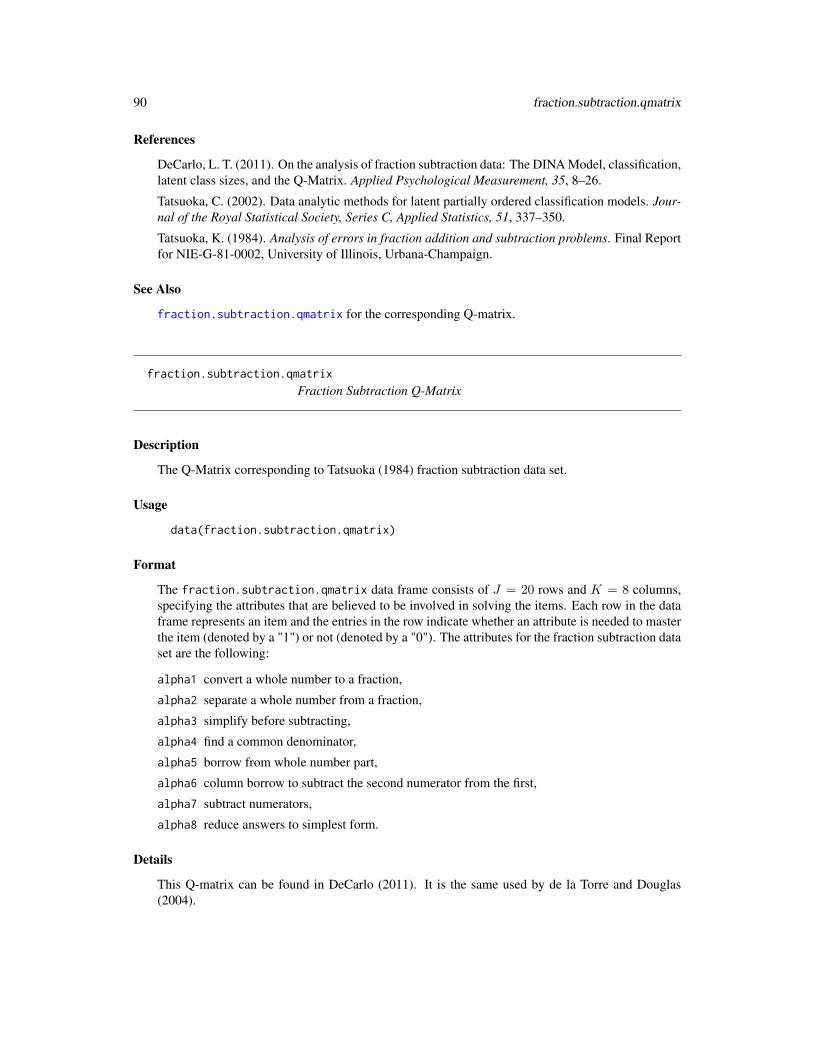
90 fraction.subtraction.qmatrix

References

DeCarlo, L. T. (2011). On the analysis of fraction subtraction data: The DINA Model, classification,latent class sizes, and the Q-Matrix. Applied Psychological Measurement, 35, 8–26.

Tatsuoka, C. (2002). Data analytic methods for latent partially ordered classification models. Jour-nal of the Royal Statistical Society, Series C, Applied Statistics, 51, 337–350.

Tatsuoka, K. (1984). Analysis of errors in fraction addition and subtraction problems. Final Reportfor NIE-G-81-0002, University of Illinois, Urbana-Champaign.

See Also

fraction.subtraction.qmatrix for the corresponding Q-matrix.

fraction.subtraction.qmatrix

Fraction Subtraction Q-Matrix

Description

The Q-Matrix corresponding to Tatsuoka (1984) fraction subtraction data set.

Usage

data(fraction.subtraction.qmatrix)

Format

The fraction.subtraction.qmatrix data frame consists of J = 20 rows and K = 8 columns,specifying the attributes that are believed to be involved in solving the items. Each row in the dataframe represents an item and the entries in the row indicate whether an attribute is needed to masterthe item (denoted by a "1") or not (denoted by a "0"). The attributes for the fraction subtraction dataset are the following:

alpha1 convert a whole number to a fraction,

alpha2 separate a whole number from a fraction,

alpha3 simplify before subtracting,

alpha4 find a common denominator,

alpha5 borrow from whole number part,

alpha6 column borrow to subtract the second numerator from the first,

alpha7 subtract numerators,

alpha8 reduce answers to simplest form.

Details

This Q-matrix can be found in DeCarlo (2011). It is the same used by de la Torre and Douglas(2004).

gdd 91

Source

DeCarlo, L. T. (2011). On the analysis of fraction subtraction data: The DINA Model, classification,latent class sizes, and the Q-Matrix. Applied Psychological Measurement, 35, 8–26.

References

de la Torre, J. and Douglas, J. (2004). Higher-order latent trait models for cognitive diagnosis.Psychometrika, 69, 333–353.

Tatsuoka, C. (2002). Data analytic methods for latent partially ordered classification models. Jour-nal of the Royal Statistical Society, Series C, Applied Statistics, 51, 337–350.

Tatsuoka, K. (1984) Analysis of errors in fraction addition and subtraction problems. Final Reportfor NIE-G-81-0002, University of Illinois, Urbana-Champaign.

gdd Generalized Distance Discriminating Method

Description

Performs the generalized distance discriminating method (GDD; Sun, Xin, Zhang, & de la Torre,2013) for dichotomous data which is a method for classifying students into skill profiles based on apreliminary unidimensional calibration.

Usage

gdd(data, q.matrix, theta, b, a, skillclasses=NULL)

Arguments

data Data frame with N × J item responses

q.matrix The Q-matrix

theta Estimated person ability

b Estimated item intercept from a 2PL model (see Details)

a Estimated item slope from a 2PL model (see Details)

skillclasses Optional matrix of skill classes used for estimation

Details

Note that the parameters in the arguments follow the item response model

logitP (Xnj = 1|θn) = bj + ajθn

which is employed in the gdm function.

92 gdina

Value


skillclass.est Estimated skill class

distmatrix Distances for every person and every skill class

skillspace Used skill space for estimation

theta Used person parameter estimate

References

Sun, J., Xin, T., Zhang, S., & de la Torre, J. (2013). A polytomous extension of the generalizeddistance discriminating method. Applied Psychological Measurement, 37, 503-521.

Examples

############################################################################## EXAMPLE 1: GDD for sim.dina#############################################################################


data <- sim.dinaq.matrix <- sim.qmatrix

# estimate 1PL (use irtmodel="2PL" for 2PL estimation)mod <- CDM::gdm( data, irtmodel="1PL", theta.k=seq(-6,6,len=21),

decrease.increments=TRUE, conv=.001, globconv=.001)# extract item parameters in parametrization b + a*thetab <- mod$b[,1]a <- mod$a[,,1]# extract person parameter estimatetheta <- mod$person$EAP.F1

# generalized distance discriminating methodres <- CDM::gdd( data, q.matrix, theta=theta, b=b, a=a )

gdina Estimating the Generalized DINA (GDINA) Model

Description

This function implements the generalized DINA model for dichotomous attributes (GDINA; de laTorre, 2011) and polytomous attributes (pGDINA; Chen & de la Torre, 2013, 2018). In addition,multiple group estimation is also possible using the gdina function. This function also allows forthe estimation of a higher order GDINA model (de la Torre & Douglas, 2004). Polytomous itemresponses are treated by specifying a sequential GDINA model (Ma & de la Torre, 2016; Tutz,

gdina 93

1997). The simulataneous modeling of skills and misconceptions (bugs) can be also estimatedwithin the GDINA framework (see Kuo, Chen & de la Torre, 2018; see argument rule).

The estimation can also be conducted by posing monotonocity constraints (Hong, Chang, & Tsai,2016) using the argument mono.constr. Moreover, regularization methods SCAD, lasso, ridge,SCAD-L2 and truncated L1 penalty (TLP) for item parameters can be employed (Xu & Shang,2018).

Normally distributed priors can be specified for item parameters (item intercepts and item slopes).Note that (for convenience) the prior specification holds simultaneously for all items.

Usage

gdina(data, q.matrix, skillclasses=NULL, conv.crit=0.0001, dev.crit=.1, maxit=1000,linkfct="identity", Mj=NULL, group=NULL, invariance=TRUE,method=NULL,delta.init=NULL, delta.fixed=NULL, delta.designmatrix=NULL,

delta.basispar.lower=NULL, delta.basispar.upper=NULL, delta.basispar.init=NULL,zeroprob.skillclasses=NULL, attr.prob.init=NULL, reduced.skillspace=NULL,reduced.skillspace.method=2, HOGDINA=-1, Z.skillspace=NULL,weights=rep(1, nrow(data)), rule="GDINA", bugs=NULL, regular_lam=0,regular_type="none", regular_alpha=NA, regular_tau=NA, regular_weights=NULL,mono.constr=FALSE, prior_intercepts=NULL, prior_slopes=NULL, progress=TRUE,progress.item=FALSE, mstep_iter=10, mstep_conv=1E-4, increment.factor=1.01,fac.oldxsi=0, max.increment=.3, avoid.zeroprobs=FALSE, seed=0,save.devmin=TRUE, calc.se=TRUE, se_version=1, PEM=TRUE, PEM_itermax=maxit,

cd=FALSE, cd_steps=1, mono_maxiter=10, freq_weights=FALSE, optimizer="CDM", ...)

## S3 method for class 'gdina'summary(object, digits=4, file=NULL, ...)

## S3 method for class 'gdina'plot(x, ask=FALSE, ...)

## S3 method for class 'gdina'print(x, ...)

Arguments

data A required N × J data matrix containing integer responses, 0, 1, ..., K. Polyto-mous item responses are treated by the sequential GDINA model. NA values areallowed.

q.matrix A required integer J×K matrix containing attributes not required or required, 0or 1, to master the items in case of dichotomous attributes or integers in case ofpolytomous attributes. For polytomous item responses the Q-matrix must alsoinclude the item name and item category, see Example 11.

skillclasses An optional matrix for determining the skill space. The argument can be used ifa user wants less than 2K skill classes.

conv.crit Convergence criterion for maximum absolute change in item parameters

dev.crit Convergence criterion for maximum absolute change in deviance

94 gdina

maxit Maximum number of iterations

linkfct A string which indicates the link function for the GDINA model. Options are"identity" (identity link), "logit" (logit link) and "log" (log link). The de-fault is the "identity" link. Note that the link function is chosen for the wholemodel (i.e. for all items).

Mj A list of design matrices and labels for each item. The definition of Mj followsthe definition of Mj in de la Torre (2011). Please study the value Mj of thefunction in default analysis. See Example 3.

group A vector of group identifiers for multiple group estimation. Default is NULL (nomultiple group estimation).

invariance Logical indicating whether invariance of item parameters is assumed for multi-ple group models. If a subset of items should be treated as noninvariant, theninvariance can be a vector of item names.

method Estimation method for item parameters (see) (de la Torre, 2011). The default"WLS" weights probabilities attribute classes by a weighting matrix Wj of ex-pected frequencies, whereas the method "ULS" perform unweighted least squaresestimation on expected frequencies. The method "ML" directly maximizes thelog-likelihood function. The "ML" method is a bit slower but can be much morestable, especially in the case of the RRUM model. Only for the RRUM model,the default is changed to method="ML" if not specified otherwise.

delta.init List with initial δ parameters

delta.fixed List with fixed δ parameters. For free estimated parameters NA must be declared.delta.designmatrix

A design matrix for restrictions on delta. See Example 4.delta.basispar.lower

Lower bounds for delta basis parameters.delta.basispar.upper

Upper bounds for delta basis parameters.delta.basispar.init

An optional vector of starting values for the basis parameters of delta. This argu-ment only applies when using a designmatrix for delta, i.e. delta.designmatrixis not NULL.



attr.prob.init Initial probabilities of skill distribution.reduced.skillspace

A logical which indicates if the latent class skill space dimension should bereduced (see Xu & von Davier, 2008). The default is NULL which applies skillspace reduction for more than four skills. The dimensional reduction is only welldefined for more than three skills. If the argument zeroprob.skillclasses isnot NULL, then reduced.skillspace is set to FALSE.

reduced.skillspace.method

Computation method for skill space reduction in case of reduced.skillspace=TRUE.The default is 2 which is computationally more efficient but introduced in CDM

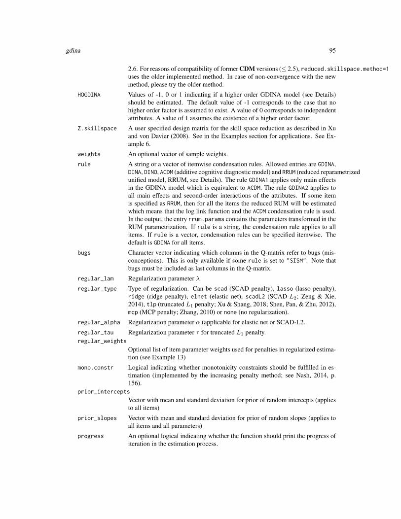
gdina 95

2.6. For reasons of compatibility of former CDM versions (≤ 2.5), reduced.skillspace.method=1uses the older implemented method. In case of non-convergence with the newmethod, please try the older method.

HOGDINA Values of -1, 0 or 1 indicating if a higher order GDINA model (see Details)should be estimated. The default value of -1 corresponds to the case that nohigher order factor is assumed to exist. A value of 0 corresponds to independentattributes. A value of 1 assumes the existence of a higher order factor.

Z.skillspace A user specified design matrix for the skill space reduction as described in Xuand von Davier (2008). See in the Examples section for applications. See Ex-ample 6.

weights An optional vector of sample weights.

rule A string or a vector of itemwise condensation rules. Allowed entries are GDINA,DINA, DINO, ACDM (additive cognitive diagnostic model) and RRUM (reduced reparametrizedunified model, RRUM, see Details). The rule GDINA1 applies only main effectsin the GDINA model which is equivalent to ACDM. The rule GDINA2 applies toall main effects and second-order interactions of the attributes. If some itemis specified as RRUM, then for all the items the reduced RUM will be estimatedwhich means that the log link function and the ACDM condensation rule is used.In the output, the entry rrum.params contains the parameters transformed in theRUM parametrization. If rule is a string, the condensation rule applies to allitems. If rule is a vector, condensation rules can be specified itemwise. Thedefault is GDINA for all items.

bugs Character vector indicating which columns in the Q-matrix refer to bugs (mis-conceptions). This is only available if some rule is set to "SISM". Note thatbugs must be included as last columns in the Q-matrix.


regular_type Type of regularization. Can be scad (SCAD penalty), lasso (lasso penalty),ridge (ridge penalty), elnet (elastic net), scadL2 (SCAD-L2; Zeng & Xie,2014), tlp (truncated L1 penalty; Xu & Shang, 2018; Shen, Pan, & Zhu, 2012),mcp (MCP penalty; Zhang, 2010) or none (no regularization).

regular_alpha Regularization parameter α (applicable for elastic net or SCAD-L2.

regular_tau Regularization parameter τ for truncated L1 penalty.regular_weights

Optional list of item parameter weights used for penalties in regularized estima-tion (see Example 13)

mono.constr Logical indicating whether monotonicity constraints should be fulfilled in es-timation (implemented by the increasing penalty method; see Nash, 2014, p.156).

prior_intercepts

Vector with mean and standard deviation for prior of random intercepts (appliesto all items)

prior_slopes Vector with mean and standard deviation for prior of random slopes (applies toall items and all parameters)


96 gdina

progress.item An optional logical indicating whether item wise progress should be displayed

mstep_iter Number of iterations in M-step if method="ML".

mstep_conv Convergence criterion in M-step if method="ML".increment.factor

A factor larger than 1 (say 1.1) to control maximum increments in item param-eters. This parameter can be used in case of nonconvergence.

fac.oldxsi A convergence acceleration factor between 0 and 1 which defines the weight ofpreviously estimated values in current parameter updates.

max.increment Maximum size of change in increments in M steps of EM algorithm whenmethod="ML" is used.

avoid.zeroprobs

An optional logical indicating whether for estimating item parameters probabil-ities occur. Especially if not a skill classes are used, it is recommended to switchthe argument to TRUE.

seed Simulation seed for initial parameters. A value of zero corresponds to determin-istic starting values, an integer value different from zero to random initial valueswith set.seed(seed).

save.devmin An optional logical indicating whether intermediate estimates should be savedcorresponding to minimal deviance. Setting the argument to FALSE could helpfor preventing working memory overflow.

calc.se Optional logical indicating whether standard errors should be calculated.

se_version Integer for calculation method of standard errors. se_version=1 is based on theobserved log likelihood and included since CDM 5.1 and is the default. Com-parability with previous CDM versions can be obtained with se_version=0.

PEM Logical indicating whether the P-EM acceleration should be applied (Berlinet &Roland, 2012).

PEM_itermax Number of iterations in which the P-EM method should be applied.

cd Logical indicating whether coordinate descent algorithm should be used.

cd_steps Number of steps for each parameter in coordinate descent algorithm

mono_maxiter Maximum number of iterations for fulfilling the monotonicity constraint

freq_weights Logical indicating whether frequency weights should be used. Default is FALSE.

optimizer String indicating which optimizer should be used in M-step estimation in case ofmethod="ML". The internal optimizer of CDM can be requested by optimizer="CDM".The optimization with stats::optim can be requested by optimizer="optim".For the RRUM model, it is always chosen optimizer="optim".

object A required object of class gdina, obtained from a call to the function gdina.

digits Number of digits after decimal separator to display.

file Optional file name for a file in which summary should be sinked.

x A required object of class gdina

ask A logical indicating whether every separate item should be displayed in plot.gdina

... Optional parameters to be passed to or from other methods will be ignored.

gdina 97

Details

The estimation is based on an EM algorithm as described in de la Torre (2011). Item parameters arecontained in the delta vector which is a list where the jth entry corresponds to item parameters ofthe jth item.The following description refers to the case of dichotomous attributes. For using polytomous at-tributes see Chen and de la Torre (2013) and Example 7 for a definition of the Q-matrix. In thiscase, Qik = l means that the ith item requires the mastery (at least) of level l of attribute k.Assume that two skills α1 and α2 are required for mastering item j. Then the GDINA model canbe written as

g[P (Xnj = 1|αn)] = δj0 + δj1αn1 + δj2αn2 + δj12αn1αn2

which is a two-way GDINA-model (the rule="GDINA2" specification) with a link function g (whichcan be the identity, logit or logarithmic link). If the specification ACDM is chosen, then δj12 = 0.The DINA model (rule="DINA") assumes δj1 = δj2 = 0.For the reduced RUM model (rule="RRUM"), the item response model is

P (Xnj = 1|αn) = π∗i · r

1−αi1i1 · r1−αi2

i2

From this equation, it is obvious, that this model is equivalent to an additive model (rule="ACDM")with a logarithmic link function (linkfct="log").If a reduced skillspace (reduced.skillspace=TRUE) is employed, then the logarithm of probabilitydistribution of the attributes is modeled as a log-linear model:

logP [(αn1, αn2, . . . , αnK)] = γ0 +∑k

γkαnk +∑k<l

γklαnkαnl

If a higher order DINA model is assumed (HOGDINA=1), then a higher order factor θn for the at-tributes is assumed:

P (αnk = 1|θn) = Φ(akθn + bk)

For HOGDINA=0, all attributes αnk are assumed to be independent of each other:

P [(αn1, αn2, . . . , αnK)] =∏k

P (αnk)

Note that the noncompensatory reduced RUM (NC-RRUM) according to Rupp and Templin (2008)is the GDINA model with the arguments rule="ACDM" and linkfct="log". NC-RRUM can alsobe obtained by choosing rule="RRUM".The compensatory RUM (C-RRUM) can be obtained by using the arguments rule="ACDM" andlinkfct="logit".The cognitive diagnosis model for identifying skills and misconceptions (SISM; Kuo, Chen & de laTorre, 2018) can be estimated with rule="SISM" (see Example 12).The gdina function internally parameterizes the GDINA model as

g[P (Xnj = 1|αn)] = Mj(αn)δj

with item-specific design matrices Mj(αn) and item parameters δj . Only those attributes are mod-elled which correspond to non-zero entries in the Q-matrix. Because the Q-matrix (in q.matrix)and the design matrices (in M_j; see Example 3) can be specified by the user, several cognitivediagnosis models can be estimated. Therefore, some additional extensions of the DINA model canalso be estimated using the gdina function. These models include the DINA model with multiplestrategies (Huo & de la Torre, 2014)

98 gdina

Value

An object of class gdina with following entries

coef Data frame of item parameters

delta List with basis item parameters

se.delta Standard errors of basis item parameters

probitem Data frame with model implied conditional item probabilities P (Xi = 1|α).These probabilities are displayed in plot.gdina.

itemfit.rmsea The RMSEA item fit index (see itemfit.rmsea).


loglike Log-likelihood

deviance Deviance

G Number of groups

N Sample size

AIC AIC

BIC BIC

CAIC CAIC

Npars Total number of parameters

Nipar Number of item parameters

Nskillpar Number of parameters for skill class distribution

Nskillclasses Number of skill classes

varmat.delta Covariance matrix of δ item parameters

posterior Individual posterior distribution

like Individual likelihood

data Original data


pattern Individual patterns, individual MLE and MAP classifications and their corre-sponding probabilities

attribute.patt Probabilities of skill classes

skill.patt Marginal skill probabilities

subj.pattern Individual subject patternattribute.patt.splitted

Splitted attribute pattern

pjk Array of item response probabilities

Mj Design matrix Mj in GDINA algorithm (see de la Torre, 2011)

Aj Design matrix Aj in GDINA algorithm (see de la Torre, 2011)

rule Used condensation rules

linkfct Used link function

gdina 99

delta.designmatrix

Designmatrix for item parametersreduced.skillspace

A logical if skillspace reduction was performed

Z.skillspace Design matrix for skillspace reduction

beta Parameters δ for skill class representation

covbeta Standard errors of δ parameters

iter Number of iterations

rrum.params Parameters in the parametrization of the reduced RUM model if rule="RRUM".

group.stat Group statistics (sample sizes, group labels)

HOGDINA The used value of HOGDINA

mono.constr Monotonicity constraint

regularization Logical indicating whether regularization is used

regular_lam Regularization parameternumb_bound_mono

Number of items with parameters at boundary of monotonicity constraintsnumb_regular_pars

Number of regularized item parametersdelta_regularized

List indicating which item parameters are regularized

cd_algorithm Logical indicating whether coordinate descent algorithm is used

cd_steps Number of steps for each parameter in coordinate descent algorithm

seed Used simulation seed

a.attr Attribute parameters ak in case of HOGDINA>=0

b.attr Attribute parameters bk in case of HOGDINA>=0

attr.rf Attribute response functions. This matrix contains all ak and bk parameters


control Optimization parameters used in estimation

partable Parameter table for gdina function

polychor Group-wise matrices with polychoric correlations

sequential Logical indicating whether a sequential GDINA model is applied for polyto-mous item responses

... Further values

Note

The function din does not allow for multiple group estimation. Use this gdina function instead andchoose the appropriate rule="DINA" as an argument.

Standard error calculation in analyses which use sample weights or designmatrix for delta parame-ters (delta.designmatrix!=NULL) is not yet correctly implemented. Please use replication meth-ods instead.

100 gdina

References

Berlinet, A. F., & Roland, C. (2012). Acceleration of the EM algorithm: P-EM versus epsilonalgorithm. Computational Statistics & Data Analysis, 56(12), 4122-4137.


Chen, J., & de la Torre, J. (2018). Introducing the general polytomous diagnosis modeling frame-work. Frontiers in Psychology | Quantitative Psychology and Measurement, 9(1474).

de la Torre, J., & Douglas, J. A. (2004). Higher-order latent trait models for cognitive diagnosis.Psychometrika, 69, 333-353.


Hong, C. Y., Chang, Y. W., & Tsai, R. C. (2016). Estimation of generalized DINA model with orderrestrictions. Journal of Classification, 33(3), 460-484.

Huo, Y., de la Torre, J. (2014). Estimating a cognitive diagnostic model for multiple strategies viathe EM algorithm. Applied Psychological Measurement, 38, 464-485.

Kuo, B.-C., Chen, C.-H., & de la Torre, J. (2018). A cognitive diagnosis model for identifyingcoexisting skills and misconceptions. Applied Psychological Measurement, 42(3), 179-191.

Ma, W., & de la Torre, J. (2016). A sequential cognitive diagnosis model for polytomous responses.British Journal of Mathematical and Statistical Psychology, 69(3), 253-275.

Nash, J. C. (2014). Nonlinear parameter optimization using R tools. West Sussex: Wiley.

Rupp, A. A., & Templin, J. (2008). Unique characteristics of diagnostic classification models: Acomprehensive review of the current state-of-the-art. Measurement: Interdisciplinary Research andPerspectives, 6, 219-262.

Shen, X., Pan, W., & Zhu, Y. (2012). Likelihood-based selection and sharp parameter estimation.Journal of the American Statistical Association, 107, 223-232.

Tutz, G. (1997). Sequential models for ordered responses. In W. van der Linden & R. K. Hambleton.Handbook of modern item response theory (pp. 139-152). New York: Springer.

Xu, G., & Shang, Z. (2018). Identifying latent structures in restricted latent class models. Journalof the American Statistical Association, 523, 1284-1295.

Xu, X., & von Davier, M. (2008). Fitting the structured general diagnostic model to NAEP data.ETS Research Report ETS RR-08-27. Princeton, ETS.

Zeng, L., & Xie, J. (2014). Group variable selection via SCAD-L2. Statistics, 48, 49-66.

Zhang, C.-H. (2010). Nearly unbiased variable selection under minimax concave penalty. Annalsof Statistics, 38, 894-942.

See Also

See also the din function (for DINA and DINO estimation).

For assessment of model fit see modelfit.cor.din and anova.gdina.


See sim.gdina for simulating the GDINA model.

See gdina.wald for a Wald test for testing the DINA and ACDM rules at the item-level.

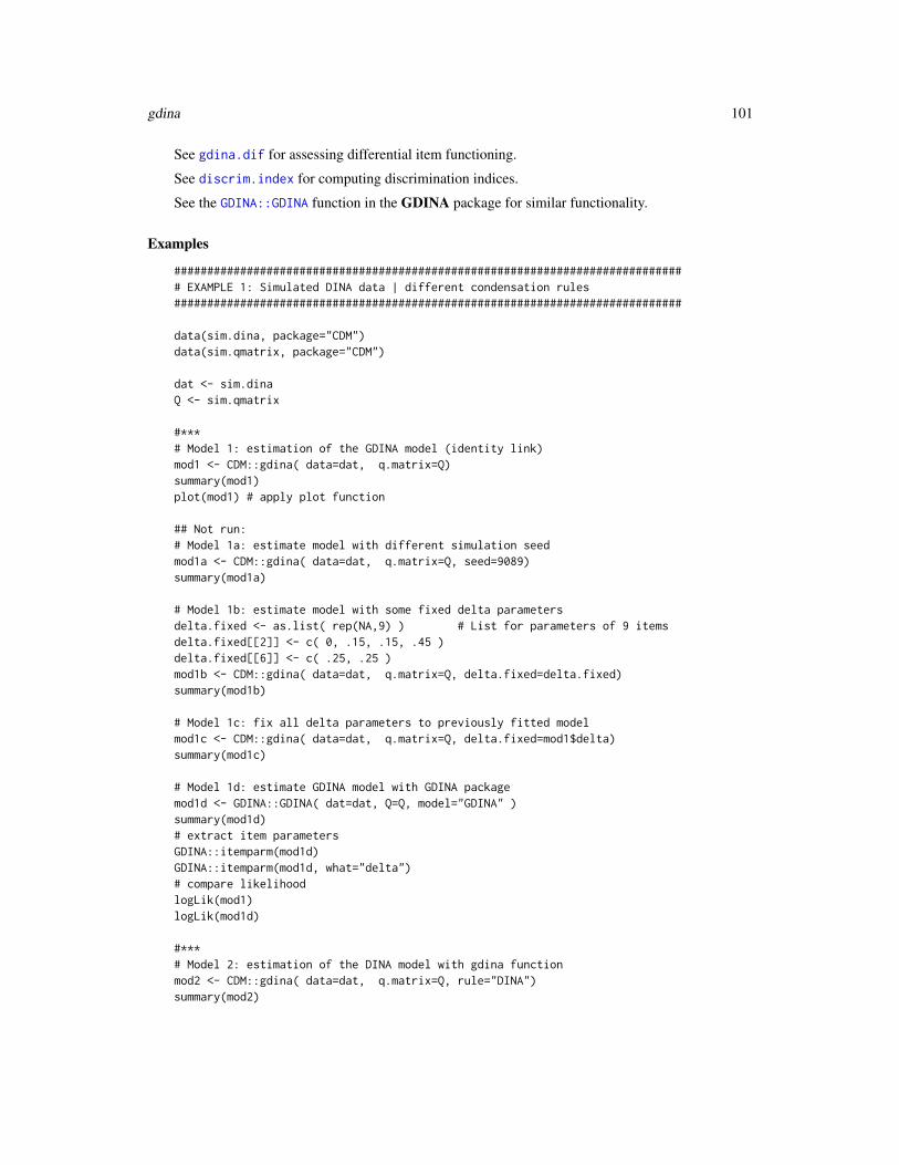
gdina 101

See gdina.dif for assessing differential item functioning.

See discrim.index for computing discrimination indices.

See the GDINA::GDINA function in the GDINA package for similar functionality.

Examples

############################################################################## EXAMPLE 1: Simulated DINA data | different condensation rules#############################################################################


dat <- sim.dinaQ <- sim.qmatrix

#***# Model 1: estimation of the GDINA model (identity link)mod1 <- CDM::gdina( data=dat, q.matrix=Q)summary(mod1)plot(mod1) # apply plot function

## Not run:# Model 1a: estimate model with different simulation seedmod1a <- CDM::gdina( data=dat, q.matrix=Q, seed=9089)summary(mod1a)

# Model 1b: estimate model with some fixed delta parametersdelta.fixed <- as.list( rep(NA,9) ) # List for parameters of 9 itemsdelta.fixed[[2]] <- c( 0, .15, .15, .45 )delta.fixed[[6]] <- c( .25, .25 )mod1b <- CDM::gdina( data=dat, q.matrix=Q, delta.fixed=delta.fixed)summary(mod1b)

# Model 1c: fix all delta parameters to previously fitted modelmod1c <- CDM::gdina( data=dat, q.matrix=Q, delta.fixed=mod1$delta)summary(mod1c)

# Model 1d: estimate GDINA model with GDINA packagemod1d <- GDINA::GDINA( dat=dat, Q=Q, model="GDINA" )summary(mod1d)# extract item parametersGDINA::itemparm(mod1d)GDINA::itemparm(mod1d, what="delta")# compare likelihoodlogLik(mod1)logLik(mod1d)

#***# Model 2: estimation of the DINA model with gdina functionmod2 <- CDM::gdina( data=dat, q.matrix=Q, rule="DINA")summary(mod2)

102 gdina

plot(mod2)

#***# Model 2b: compare results with din functionmod2b <- CDM::din( data=dat, q.matrix=Q, rule="DINA")summary(mod2b)

# Model 2: estimation of the DINO model with gdina functionmod3 <- CDM::gdina( data=dat, q.matrix=Q, rule="DINO")summary(mod3)

#***# Model 4: DINA model with logit linkmod4 <- CDM::gdina( data=dat, q.matrix=Q, rule="DINA", linkfct="logit" )summary(mod4)

#***# Model 5: DINA model log linkmod5 <- CDM::gdina( data=dat, q.matrix=Q, rule="DINA", linkfct="log")summary(mod5)

#***# Model 6: RRUM modelmod6 <- CDM::gdina( data=dat, q.matrix=Q, rule="RRUM")summary(mod6)

#***# Model 7: Higher order GDINA modelmod7 <- CDM::gdina( data=dat, q.matrix=Q, HOGDINA=1)summary(mod7)

#***# Model 8: GDINA model with independent attributesmod8 <- CDM::gdina( data=dat, q.matrix=Q, HOGDINA=0)summary(mod8)

#***# Model 9: Estimating the GDINA model with monotonicity constraintsmod9 <- CDM::gdina( data=dat, q.matrix=Q, rule="GDINA",

mono.constr=TRUE, linkfct="logit")summary(mod9)

#***# Model 10: Estimating the ACDM model with SCAD penalty and regularization# parameter of .05mod10 <- CDM::gdina( data=dat, q.matrix=Q, rule="ACDM",

linkfct="logit", regular_type="scad", regular_lam=.05 )summary(mod10)

#***# Model 11: Estimation of GDINA model with prior distributions

# N(0,10^2) prior for item intercepts

gdina 103

prior_intercepts <- c(0,10)# N(0,1^2) prior for item slopesprior_slopes <- c(0,1)# estimate modelmod11 <- CDM::gdina( data=dat, q.matrix=Q, rule="GDINA",

prior_intercepts=prior_intercepts, prior_slopes=prior_slopes)summary(mod11)

############################################################################## EXAMPLE 2: Simulated DINO data# additive cognitive diagnosis model with different link functions#############################################################################

data(sim.dino, package="CDM")data(sim.matrix, package="CDM")

dat <- sim.dinoQ <- sim.qmatrix

#***# Model 1: additive cognitive diagnosis model (ACDM; identity link)mod1 <- CDM::gdina( data=dat, q.matrix=Q, rule="ACDM")summary(mod1)

#***# Model 2: ACDM logit linkmod2 <- CDM::gdina( data=dat, q.matrix=Q, rule="ACDM", linkfct="logit")summary(mod2)

#***# Model 3: ACDM log linkmod3 <- CDM::gdina( data=dat, q.matrix=Q, rule="ACDM", linkfct="log")summary(mod3)

#***# Model 4: Different condensation rules per itemI <- 9 # number of itemsrule <- rep( "GDINA", I )rule[1] <- "DINO" # 1st item: DINO modelrule[7] <- "GDINA2" # 7th item: GDINA model with first- and second-order interactionsrule[8] <- "ACDM" # 8ht item: additive CDMrule[9] <- "DINA" # 9th item: DINA modelmod4 <- CDM::gdina( data=dat, q.matrix=Q, rule=rule )summary(mod4)

############################################################################## EXAMPLE 3: Model with user-specified design matrices#############################################################################


dat <- sim.dino

104 gdina

Q <- sim.qmatrix

# do a preliminary analysis and modify obtained design matricesmod0 <- CDM::gdina( data=dat, q.matrix=Q, maxit=1)

# extract default design matricesMj <- mod0$MjMj.user <- Mj # these user defined design matrices are modified.#~~~ For the second item, the following model should hold# X1 ~ V2 + V2*V3mj <- Mj[[2]][[1]]mj.lab <- Mj[[2]][[2]]mj <- mj[,-3]mj.lab <- mj.lab[-3]Mj.user[[2]] <- list( mj, mj.lab )# [[1]]# [,1] [,2] [,3]# [1,] 1 0 0# [2,] 1 1 0# [3,] 1 0 0# [4,] 1 1 1# [[2]]# [1] "0" "1" "1-2"#~~~ For the eight item an equality constraint should hold# X8 ~ a*V2 + a*V3 + V2*V3mj <- Mj[[8]][[1]]mj.lab <- Mj[[8]][[2]]mj[,2] <- mj[,2] + mj[,3]mj <- mj[,-3]mj.lab <- c("0", "1=2", "1-2" )Mj.user[[8]] <- list( mj, mj.lab )Mj.user[[8]]

## [[1]]## [,1] [,2] [,3]## [1,] 1 0 0## [2,] 1 1 0## [3,] 1 1 0## [4,] 1 2 1#### [[2]]## [1] "0" "1=2" "1-2"

mod <- CDM::gdina( data=dat, q.matrix=Q,Mj=Mj.user, maxit=200 )

summary(mod)

############################################################################## EXAMPLE 4: Design matrix for delta parameters#############################################################################


#~~~ estimate an initial model

gdina 105

mod0 <- CDM::gdina( data=dat, q.matrix=Q, rule="ACDM", maxit=1)# extract coefficientsc0 <- mod0$coefI <- 9 # number of itemsdelta.designmatrix <- matrix( 0, nrow=nrow(c0), ncol=nrow(c0) )diag( delta.designmatrix) <- 1# set intercept of item 1 and item 3 equal to each otherdelta.designmatrix[ 7, 1 ] <- 1 ; delta.designmatrix[,7] <- 0# set loading of V1 of item1 and item 3 equaldelta.designmatrix[ 8, 2 ] <- 1 ; delta.designmatrix[,8] <- 0delta.designmatrix <- delta.designmatrix[, -c(7:8) ]

# exclude original parameters with indices 7 and 8

#***# Model 1: ACDM with designmatrixmod1 <- CDM::gdina( data=dat, q.matrix=Q, rule="ACDM",

delta.designmatrix=delta.designmatrix )summary(mod1)

#***# Model 2: Same model, but with logit link instead of identity link functionmod2 <- CDM::gdina( data=dat, q.matrix=Q, rule="ACDM",

delta.designmatrix=delta.designmatrix, linkfct="logit")summary(mod2)

############################################################################## EXAMPLE 5: Multiple group estimation#############################################################################

# simulate dataset.seed(9279)N1 <- 200 ; N2 <- 100 # group sizesI <- 10 # number of itemsq.matrix <- matrix(0,I,2) # create Q-matrixq.matrix[1:7,1] <- 1 ; q.matrix[ 5:10,2] <- 1# simulate first groupdat1 <- CDM::sim.din(N1, q.matrix=q.matrix, mean=c(0,0) )$dat# simulate second groupdat2 <- CDM::sim.din(N2, q.matrix=q.matrix, mean=c(-.3, -.7) )$dat# merge datadat <- rbind( dat1, dat2 )# group indicatorgroup <- c( rep(1,N1), rep(2,N2) )

# estimate GDINA model with multiple groups assuming invariant item parametersmod1 <- CDM::gdina( data=dat, q.matrix=q.matrix, group=group)summary(mod1)

# estimate DINA model with multiple groups assuming invariant item parametersmod2 <- CDM::gdina( data=dat, q.matrix=q.matrix, group=group, rule="DINA")summary(mod2)

# estimate GDINA model with noninvariant item parameters

106 gdina

mod3 <- CDM::gdina( data=dat, q.matrix=q.matrix, group=group, invariance=FALSE)summary(mod3)

# estimate GDINA model with some invariant item parameters (I001, I006, I008)mod4 <- CDM::gdina( data=dat, q.matrix=q.matrix, group=group,

invariance=c("I001", "I006","I008") )

#--- model comparisonIRT.compareModels(mod1,mod2,mod3,mod4)

# estimate GDINA model with non-invariant item parameters except for the# items I001, I006, I008mod5 <- CDM::gdina( data=dat, q.matrix=q.matrix, group=group,

invariance=setdiff( colnames(dat), c("I001", "I006","I008") ) )

############################################################################## EXAMPLE 6: User specified reduced skill space#############################################################################

# Some correlations between attributes should be set to zero.q.matrix <- expand.grid( c(0,1), c(0,1), c(0,1), c(0,1) )colnames(q.matrix) <- colnames( paste("Attr", 1:4,sep=""))q.matrix <- q.matrix[ -1, ]Sigma <- matrix( .5, nrow=4, ncol=4 )diag(Sigma) <- 1Sigma[3,2] <- Sigma[2,3] <- 0 # set correlation of attribute A2 and A3 to zerodat <- CDM::sim.din( N=1000, q.matrix=q.matrix, Sigma=Sigma)$dat

#~~~ Step 1: initial estimationmod1a <- CDM::gdina( data=dat, q.matrix=q.matrix, maxit=1, rule="DINA")# estimate also "full" modelmod1 <- CDM::gdina( data=dat, q.matrix=q.matrix, rule="DINA")

#~~~ Step 2: modify designmatrix for reduced skillspaceZ.skillspace <- data.frame( mod1a$Z.skillspace )# set correlations of A2/A4 and A3/A4 to zerovars <- c("A2_A3","A2_A4")for (vv in vars){ Z.skillspace[,vv] <- NULL }

#~~~ Step 3: estimate model with reduced skillspacemod2 <- CDM::gdina( data=dat, q.matrix=q.matrix,

Z.skillspace=Z.skillspace, rule="DINA")

#~~~ eliminate all covariancesZ.skillspace <- data.frame( mod1$Z.skillspace )colnames(Z.skillspace)Z.skillspace <- Z.skillspace[, -grep( "_", colnames(Z.skillspace),fixed=TRUE)]colnames(Z.skillspace)

mod3 <- CDM::gdina( data=dat, q.matrix=q.matrix,Z.skillspace=Z.skillspace, rule="DINA")

summary(mod1)summary(mod2)

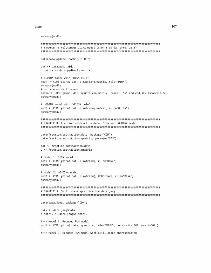
gdina 107

summary(mod3)

############################################################################## EXAMPLE 7: Polytomous GDINA model (Chen & de la Torre, 2013)#############################################################################

data(data.pgdina, package="CDM")

dat <- data.pgdina$datq.matrix <- data.pgdina$q.matrix

# pGDINA model with "DINA rule"mod1 <- CDM::gdina( dat, q.matrix=q.matrix, rule="DINA")summary(mod1)# no reduced skill spacemod1a <- CDM::gdina( dat, q.matrix=q.matrix, rule="DINA",reduced.skillspace=FALSE)summary(mod1)

# pGDINA model with "GDINA rule"mod2 <- CDM::gdina( dat, q.matrix=q.matrix, rule="GDINA")summary(mod2)

############################################################################## EXAMPLE 8: Fraction subtraction data: DINA and HO-DINA model#############################################################################

data(fraction.subtraction.data, package="CDM")data(fraction.subtraction.qmatrix, package="CDM")

dat <- fraction.subtraction.dataQ <- fraction.subtraction.qmatrix

# Model 1: DINA modelmod1 <- CDM::gdina( dat, q.matrix=Q, rule="DINA")summary(mod1)

# Model 2: HO-DINA modelmod2 <- CDM::gdina( dat, q.matrix=Q, HOGDINA=1, rule="DINA")summary(mod2)

############################################################################## EXAMPLE 9: Skill space approximation data.jang#############################################################################

data(data.jang, package="CDM")

data <- data.jang$dataq.matrix <- data.jang$q.matrix

#*** Model 1: Reduced RUM modelmod1 <- CDM::gdina( data, q.matrix, rule="RRUM", conv.crit=.001, maxit=500 )

#*** Model 2: Reduced RUM model with skill space approximation

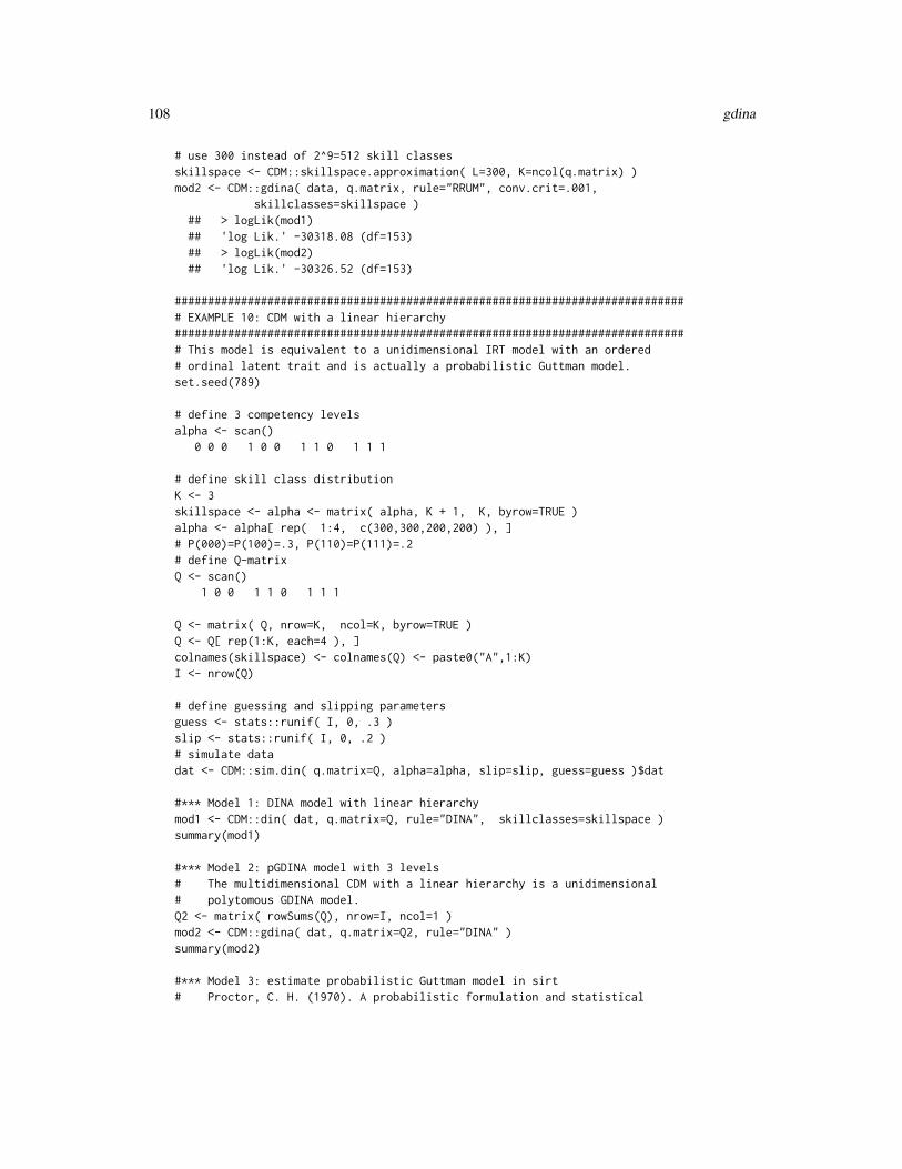
108 gdina

# use 300 instead of 2^9=512 skill classesskillspace <- CDM::skillspace.approximation( L=300, K=ncol(q.matrix) )mod2 <- CDM::gdina( data, q.matrix, rule="RRUM", conv.crit=.001,

skillclasses=skillspace )## > logLik(mod1)## 'log Lik.' -30318.08 (df=153)## > logLik(mod2)## 'log Lik.' -30326.52 (df=153)

############################################################################## EXAMPLE 10: CDM with a linear hierarchy############################################################################## This model is equivalent to a unidimensional IRT model with an ordered# ordinal latent trait and is actually a probabilistic Guttman model.set.seed(789)

# define 3 competency levelsalpha <- scan()

0 0 0 1 0 0 1 1 0 1 1 1

# define skill class distributionK <- 3skillspace <- alpha <- matrix( alpha, K + 1, K, byrow=TRUE )alpha <- alpha[ rep( 1:4, c(300,300,200,200) ), ]# P(000)=P(100)=.3, P(110)=P(111)=.2# define Q-matrixQ <- scan()

1 0 0 1 1 0 1 1 1

Q <- matrix( Q, nrow=K, ncol=K, byrow=TRUE )Q <- Q[ rep(1:K, each=4 ), ]colnames(skillspace) <- colnames(Q) <- paste0("A",1:K)I <- nrow(Q)

# define guessing and slipping parametersguess <- stats::runif( I, 0, .3 )slip <- stats::runif( I, 0, .2 )# simulate datadat <- CDM::sim.din( q.matrix=Q, alpha=alpha, slip=slip, guess=guess )$dat

#*** Model 1: DINA model with linear hierarchymod1 <- CDM::din( dat, q.matrix=Q, rule="DINA", skillclasses=skillspace )summary(mod1)

#*** Model 2: pGDINA model with 3 levels# The multidimensional CDM with a linear hierarchy is a unidimensional# polytomous GDINA model.Q2 <- matrix( rowSums(Q), nrow=I, ncol=1 )mod2 <- CDM::gdina( dat, q.matrix=Q2, rule="DINA" )summary(mod2)

#*** Model 3: estimate probabilistic Guttman model in sirt# Proctor, C. H. (1970). A probabilistic formulation and statistical

gdina 109

# analysis for Guttman scaling. Psychometrika, 35, 73-78.library(sirt)mod3 <- sirt::prob.guttman( dat, itemlevel=Q2[,1] )summary(mod3)# -> The three models result in nearly equivalent fit.

############################################################################## EXAMPLE 11: Sequential GDINA model (Ma & de la Torre, 2016)#############################################################################


#** attach datasetdat <- data.cdm04$data # polytomous item responsesq.matrix1 <- data.cdm04$q.matrix1q.matrix2 <- data.cdm04$q.matrix2

#-- DINA model with first Q-matrixmod1 <- CDM::gdina( dat, q.matrix=q.matrix1, rule="DINA")summary(mod1)#-- DINA model with second Q-matrixmod2 <- CDM::gdina( dat, q.matrix=q.matrix2, rule="DINA")#-- GDINA modelmod3 <- CDM::gdina( dat, q.matrix=q.matrix2, rule="GDINA")

#** model comparisonIRT.compareModels(mod1,mod2,mod3)

############################################################################## EXAMPLE 12: Simulataneous modeling of skills and misconceptions (Kuo et al., 2018)#############################################################################

data(data.cdm08, package="CDM")dat <- data.cdm08$dataq.matrix <- data.cdm08$q.matrix

#*** estimate modelmod <- CDM::gdina( dat0, q.matrix, rule="SISM", bugs=colnames(q.matrix)[5:7] )summary(mod)

############################################################################## EXAMPLE 13: Regularized estimation in GDINA model data.dtmr#############################################################################

data(data.dtmr, package="CDM")dat <- data.dtmr$dataq.matrix <- data.dtmr$q.matrix

#***** LASSO regularization with lambda parameter of .02mod1 <- CDM::gdina(dat, q.matrix=q.matrix, rule="GDINA", regular_lam=.02,

regular_type="lasso")summary(mod1)mod$delta_regularized

110 gdina.dif

#***** using starting values from previuos estimationdelta.init <- mod1$deltaattr.prob.init <- mod1$attr.probmod2 <- CDM::gdina(dat, q.matrix=q.matrix, rule="GDINA", regular_lam=.02, regular_type="lasso",

delta.init=delta.init, attr.prob.init=attr.prob.init)summary(mod2)

#***** final estimation fixing regularized estimates to zero and estimate all other#***** item parameters unregularizedregular_weights <- mod2$delta_regularizeddelta.init <- mod2$deltaattr.prob.init <- mod2$attr.prob

mod3 <- CDM::gdina(dat, q.matrix=q.matrix, rule="GDINA", regular_lam=1E5, regular_type="lasso",delta.init=delta.init, attr.prob.init=attr.prob.init,regular_weights=regular_weights)

summary(mod3)

## End(Not run)

gdina.dif Differential Item Functioning in the GDINA Model

Description

This function assesses item-wise differential item functioning in the GDINA model by using theWald test (de la Torre, 2011; Hou, de la Torre & Nandakumar, 2014). It is necessary that a multiplegroup GDINA model is previously fitted.

Usage

gdina.dif(object)

## S3 method for class 'gdina.dif'summary(object, ...)

Arguments

object Object of class gdina


Details

The p values are also calculated by a Holm adjustment for multiple comparisons (see p.holm inoutput difstats).

gdina.dif 111

In the case of two groups, an effect size of differential item functioning (labeled as UA (unsignedarea) in difstats value) is defined as the weighted absolute difference of item response functions.The DIF measure for item j is defined as

UAj =∑l

w(αl)|P (Xj = 1|αl, G = 1)− P (Xj = 1|αl, G = 2)|

where w(αl) = [P (αl|G = 1) + P (αl|G = 2)]/2.

Value


difstats Data frame containing results of item-wise Wald tests

coef Data frame containing all (group-wise) item parameters

delta_all List of δ vectors containing all item parameters

varmat_all List of covariance matrices of all δ item parameters

prob.exp.group List with groups and items containing expected latent class sizes and expectedprobabilities for each group and each item. Based on this information, effectsizes of differential item functioning can be calculated.

References


Hou, L., de la Torre, J., & Nandakumar, R. (2014). Differential item functioning assessment incognitive diagnostic modeling: Application of the Wald test to investigate DIF in the DINA model.Journal of Educational Measurement, 51, 98-125.

See Also

See the GDINA::dif function in the GDINA package for similar functionality.

Examples

## Not run:############################################################################## EXAMPLE 1: DIF for DINA simulated data#############################################################################

# simulate some dataset.seed(976)N <- 2000 # number of persons in a groupI <- 9 # number of itemsq.matrix <- matrix( 0, 9,2 )q.matrix[1:3,1] <- 1q.matrix[4:6,2] <- 1q.matrix[7:9,c(1,2)] <- 1# simulate first groupguess <- rep( .2, I )slip <- rep(.1, I)

112 gdina.wald

dat1 <- CDM::sim.din( N=N, q.matrix=q.matrix, guess=guess, slip=slip,mean=c(0,0) )$dat

# simulate second group with some DIF items (items 1, 7 and 8)guess[ c(1,7)] <- c(.3, .35 )slip[8] <- .25dat2 <- CDM::sim.din( N=N, q.matrix=q.matrix, guess=guess, slip=slip,

mean=c(0.4,.25) )$datgroup <- rep(1:2, each=N )dat <- rbind( dat1, dat2 )

#*** estimate multiple group GDINA modelmod1 <- CDM::gdina( dat, q.matrix=q.matrix, rule="DINA", group=group )summary(mod1)

#*** assess differential item functioningdmod1 <- CDM::gdina.dif( mod1)summary(dmod1)

## item X2 df p p.holm UA## 1 I001 10.1711 2 0.0062 0.0495 0.0428## 2 I002 1.9933 2 0.3691 1.0000 0.0276## 3 I003 0.0313 2 0.9845 1.0000 0.0040## 4 I004 0.0290 2 0.9856 1.0000 0.0044## 5 I005 2.3230 2 0.3130 1.0000 0.0142## 6 I006 1.8330 2 0.3999 1.0000 0.0159## 7 I007 40.6851 2 0.0000 0.0000 0.1184## 8 I008 6.7912 2 0.0335 0.2346 0.0710## 9 I009 1.1538 2 0.5616 1.0000 0.0180

## End(Not run)

gdina.wald Wald Statistic for Item Fit of the DINA and ACDM Rule for GDINAModel

Description

This function tests with a Wald test for the GDINA model whether a DINA or a ACDM conden-sation rule leads to a sufficient item fit compared to the saturated GDINA rule (de la Torre & Lee,2013). The Wald test is accompanied by the RMSEA fit and weighted and unweighted distancemeasures (wgtdist, uwgtdist), see Details (compare Ma, Iaconangelo, & de la Torre, 2016).

Usage

gdina.wald(object)

## S3 method for class 'gdina.wald'summary(object, digits=3,

vars=c("X2", "p", "sig", "RMSEA", "wgtdist"), ...)

gdina.wald 113

Arguments

object A fitted gdina model

digits Number of digits after decimal used for rounding.

vars Vector including variables which should be displayed in summary. See the out-put stats.


Details

Let Pj(αl) the estimated item response function for the GDINA model and P̂j(αl) the item responsemodel for the approximated model (DINA, DINO or ACDM). The unweighted distance uwgtdistas a measure of misfit is defined as

uwgtdist =1

2K

∑l

(Pj(αl)− P̂j(αl))2

The weighted distance wgtdist measures the discrepancy with respected to the probabilities wl =P (αl) of estimated skill classes

wgtdist =∑l

wl(Pj(αl)− P̂j(αl))2

Value

stats Data frame with Wald statistic for every item, corresponding p values and aRMSEA fit statistic

References

de la Torre, J., & Lee, Y. S. (2013). Evaluating the Wald test for item-level comparison of saturatedand reduced models in cognitive diagnosis. Journal of Educational Measurement, 50, 355-373.

Ma, W., Iaconangelo, C., & de la Torre, J. (2016). Model similarity, model selection, and attributeclassification. Applied Psychological Measurement, 40(3), 200-217.

See Also

See the GDINA::modelcomp function in the GDINA package for similar functionality.

Examples

## Not run:############################################################################## EXAMPLE 1: Wald test for DINA simulated data sim.dina#############################################################################


# Model 1: estimate GDINA model

114 gdm

mod1 <- CDM::gdina( sim.dina, q.matrix=sim.qmatrix, rule="GDINA")summary(mod1)

# perform Wald testres1 <- CDM::gdina.wald( mod1 )summary(res1)# -> results show that all but one item fit according to the DINA rule

# select some outputsummary(res1, vars=c("wgtdist", "p") )

## End(Not run)

gdm General Diagnostic Model

Description

This function estimates the general diagnostic model (von Davier, 2008; Xu & von Davier, 2008)which handles multidimensional item response models with ordered discrete or continuous latentvariables for polytomous item responses.

Usage

gdm( data, theta.k, irtmodel="2PL", group=NULL, weights=rep(1, nrow(data)),Qmatrix=NULL, thetaDes=NULL, skillspace="loglinear",b.constraint=NULL, a.constraint=NULL,mean.constraint=NULL, Sigma.constraint=NULL, delta.designmatrix=NULL,standardized.latent=FALSE, centered.latent=FALSE,centerintercepts=FALSE, centerslopes=FALSE,maxiter=1000, conv=1e-5, globconv=1e-5, msteps=4, convM=.0005,decrease.increments=FALSE, use.freqpatt=FALSE, progress=TRUE,PEM=FALSE, PEM_itermax=maxiter, ...)

## S3 method for class 'gdm'summary(object, file=NULL, ...)

## S3 method for class 'gdm'print(x, ...)

## S3 method for class 'gdm'plot(x, perstype="EAP", group=1, barwidth=.1, histcol=1,

cexcor=3, pchpers=16, cexpers=.7, ... )

Arguments

data An N × I matrix of polytomous item responses with categories k = 0, 1, ...,K

gdm 115

theta.k In the one-dimensional case it must be a vector. For multidimensional models ithas to be a list of skill vectors if the theta grid differs between dimensions. If not,a vector input can be supplied. If an estimated skillspace (skillspace="est"should be estimated, a vector or a matrix theta.k will be used as initial valuesof the estimated θ grid.

irtmodel The default 2PL corresponds to the model where item slopes on dimensions areequal for all item categories. If item-category slopes should be estimated, use2PLcat. If no item slopes should be estimated then 1PL can be selected. Notethat fixed item slopes can be specified in the Q-matrix (argument Qmatrix).

group An optional vector of group identifiers for multiple group estimation. For plot.gdmit is an integer indicating which group should be used for plotting.

weights An optional vector of sample weights

Qmatrix An optional array of dimension I ×D ×K which indicates pre-specified itemloadings on dimensions. The default for category k is the score k, i.e. the scoringin the (generalized) partial credit model.

thetaDes A design matrix for specifying nonlinear item response functions (see Example1, Models 4 and 5)

skillspace The parametric assumption of the skillspace. If skillspace="normal" then aunivariate or multivariate normal distribution is assumed. The default "loglinear"corresponds to log-linear smoothing of the skillspace distribution (Xu & vonDavier, 2008). If skillspace="full", then all probabilities of the skill spaceare nonparametrically estimated. If skillspace="est", then the θ distributionvectors will be estimated (see Details and Examples 4 and 5; Bartolucci, 2007).

b.constraint In this optional matrix with Cb rows and three columns, Cb item intercepts bikcan be fixed. 1st column: item index, 2nd column: category index, 3rd column:fixed item thresholds

a.constraint In this optional matrix with Ca rows and four columns, Ca item intercepts aidkcan be fixed. 1st column: item index, 2nd column: dimension index, 3rd col-umn: category index, 4th column: fixed item slopes

mean.constraint

A C × 3 matrix for constraining C means in the normal distribution assumption(skillspace="normal"). 1st column: Dimension, 2nd column: Group, 3rdcolumn: Value

Sigma.constraint

A C × 4 matrix for constraining C covariances in the normal distribution as-sumption (skillspace="normal"). 1st column: Dimension 1, 2nd column:Dimension 2, 3rd column: Group, 4th column: Value

delta.designmatrix

The design matrix of δ parameters for the reduced skillspace estimation (see Xu& von Davier, 2008)

standardized.latent

A logical indicating whether in a uni- or multidimensional model all latent vari-ables of the first group should be normally distributed and standardized. Thedefault is FALSE.

116 gdm

centered.latent

A logical indicating whether in a uni- or multidimensional model all latent vari-ables of the first group should be normally distributed and do have zero means?The default is FALSE.

centerintercepts

A logical indicating whether intercepts should be centered to have a mean of0 for all dimensions. This argument does not (yet) work properly for varyingnumbers of item categories.

centerslopes A logical indicating whether item slopes should be centered to have a mean of 1for all dimensions. This argument only works for irtmodel="2PL". The defaultis FALSE.

maxiter Maximum number of iterations

conv Convergence criterion for item parameters and distribution parameters

globconv Global deviance convergence criterion

msteps Maximum number of M steps in estimating b and a item parameters. The defaultis to use 4 M steps.

convM Convergence criterion in M stepdecrease.increments

Should in the M step the increments of a and b parameters decrease during itera-tions? The default is FALSE. If there is an increase in deviance during estimation,setting decrease.increments to TRUE is recommended.

use.freqpatt A logical indicating whether frequencies of unique item response patterns shouldbe used. In case of large data set use.freqpatt=TRUE can speed calculations(depending on the problem). Note that in this case, not all person parameters arecalculated as usual in the output.




object A required object of class gdm


x A required object of class gdm

perstype Person parameter estimate type. Can be either "EAP", "MAP" or "MLE".

barwidth Bar width in plot.gdm

histcol Color of histogram bars in plot.gdm

cexcor Font size for print of correlation in plot.gdm

pchpers Point type for scatter plot of person parameters in plot.gdm

cexpers Point size for scatter plot of person parameters in plot.gdm


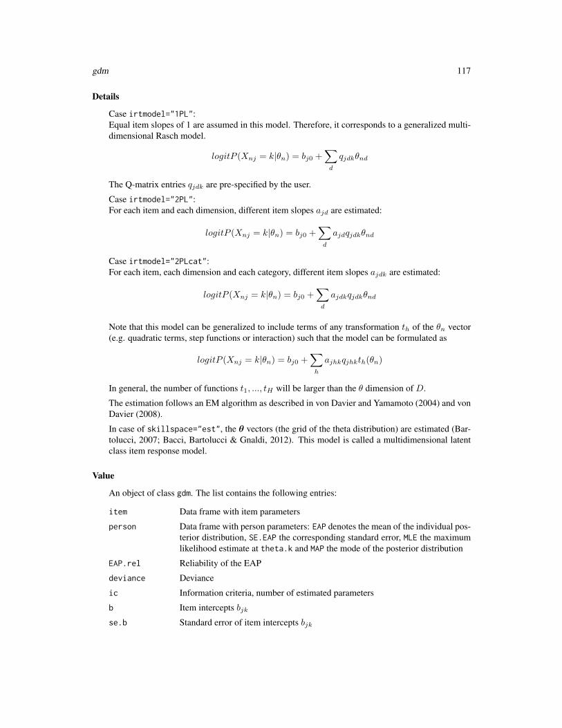
gdm 117

Details

Case irtmodel="1PL":Equal item slopes of 1 are assumed in this model. Therefore, it corresponds to a generalized multi-dimensional Rasch model.

logitP (Xnj = k|θn) = bj0 +∑d

qjdkθnd

The Q-matrix entries qjdk are pre-specified by the user.

Case irtmodel="2PL":For each item and each dimension, different item slopes ajd are estimated:


ajdqjdkθnd

Case irtmodel="2PLcat":For each item, each dimension and each category, different item slopes ajdk are estimated:


ajdkqjdkθnd

Note that this model can be generalized to include terms of any transformation th of the θn vector(e.g. quadratic terms, step functions or interaction) such that the model can be formulated as

logitP (Xnj = k|θn) = bj0 +∑h

ajhkqjhkth(θn)

In general, the number of functions t1, ..., tH will be larger than the θ dimension of D.

The estimation follows an EM algorithm as described in von Davier and Yamamoto (2004) and vonDavier (2008).

In case of skillspace="est", the θ vectors (the grid of the theta distribution) are estimated (Bar-tolucci, 2007; Bacci, Bartolucci & Gnaldi, 2012). This model is called a multidimensional latentclass item response model.

Value

An object of class gdm. The list contains the following entries:

item Data frame with item parameters

person Data frame with person parameters: EAP denotes the mean of the individual pos-terior distribution, SE.EAP the corresponding standard error, MLE the maximumlikelihood estimate at theta.k and MAP the mode of the posterior distribution

EAP.rel Reliability of the EAP

deviance Deviance

ic Information criteria, number of estimated parameters

b Item intercepts bjkse.b Standard error of item intercepts bjk

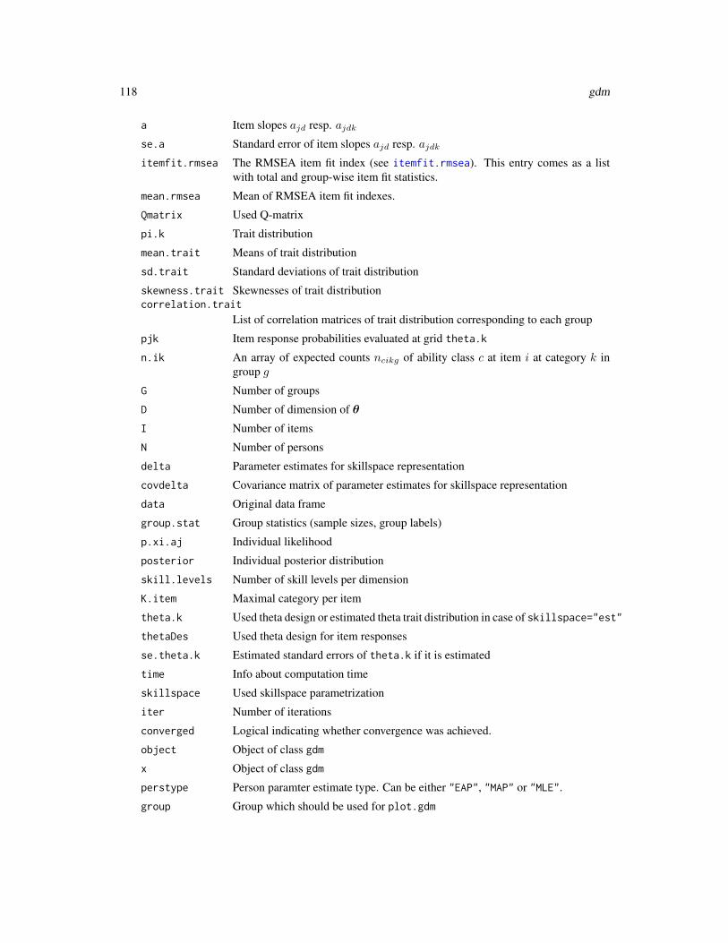
118 gdm

a Item slopes ajd resp. ajdkse.a Standard error of item slopes ajd resp. ajdkitemfit.rmsea The RMSEA item fit index (see itemfit.rmsea). This entry comes as a list

with total and group-wise item fit statistics.


Qmatrix Used Q-matrix

pi.k Trait distribution

mean.trait Means of trait distribution

sd.trait Standard deviations of trait distribution

skewness.trait Skewnesses of trait distributioncorrelation.trait

List of correlation matrices of trait distribution corresponding to each group

pjk Item response probabilities evaluated at grid theta.k

n.ik An array of expected counts ncikg of ability class c at item i at category k ingroup g

G Number of groups

D Number of dimension of θ

I Number of items

N Number of persons

delta Parameter estimates for skillspace representation

covdelta Covariance matrix of parameter estimates for skillspace representation

data Original data frame


p.xi.aj Individual likelihood


skill.levels Number of skill levels per dimension

K.item Maximal category per item

theta.k Used theta design or estimated theta trait distribution in case of skillspace="est"

thetaDes Used theta design for item responses

se.theta.k Estimated standard errors of theta.k if it is estimated

time Info about computation time

skillspace Used skillspace parametrization



object Object of class gdm

x Object of class gdm

perstype Person paramter estimate type. Can be either "EAP", "MAP" or "MLE".

group Group which should be used for plot.gdm

gdm 119

barwidth Bar width in plot.gdm

histcol Color of histogram bars in plot.gdm

cexcor Font size for print of correlation in plot.gdm

pchpers Point type for scatter plot of person parameters in plot.gdm

cexpers Point size for scatter plot of person parameters in plot.gdm


References

Bacci, S., Bartolucci, F., & Gnaldi, M. (2012). A class of multidimensional latent class IRT modelsfor ordinal polytomous item responses. arXiv preprint, arXiv:1201.4667.

Bartolucci, F. (2007). A class of multidimensional IRT models for testing unidimensionality andclustering items. Psychometrika, 72, 141-157.


von Davier, M. (2008). A general diagnostic model applied to language testing data. British Journalof Mathematical and Statistical Psychology, 61, 287-307.

von Davier, M., & Yamamoto, K. (2004). Partially observed mixtures of IRT models: An extensionof the generalized partial-credit model. Applied Psychological Measurement, 28, 389-406.


See Also

Cognitive diagnostic models for dichotomous data can be estimated with din (DINA or DINOmodel) or gdina (GDINA model, which contains many CDMs as special cases).

For assessment of model fit see modelfit.cor.din and anova.gdm.


For the estimation of the multidimensional latent class item response model see the MultiLCIRTpackage and sirt package (function sirt::rasch.mirtlc).

Examples

############################################################################## EXAMPLE 1: Fraction Dataset 1# Unidimensional Models for dichotomous data#############################################################################

data(data.fraction1, package="CDM")dat <- data.fraction1$datatheta.k <- seq( -6, 6, len=15 ) # discretized ability

#***# Model 1: Rasch model (normal distribution)mod1 <- CDM::gdm( dat, irtmodel="1PL", theta.k=theta.k, skillspace="normal",

centered.latent=TRUE)

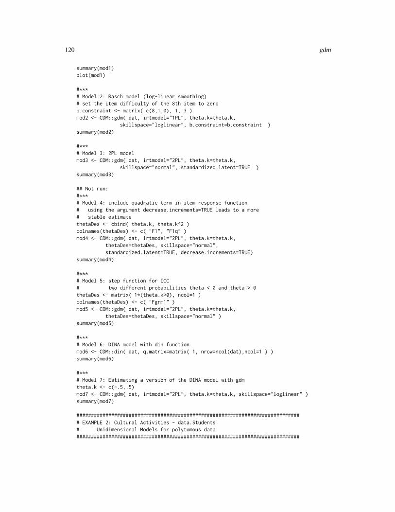
120 gdm

summary(mod1)plot(mod1)

#***# Model 2: Rasch model (log-linear smoothing)# set the item difficulty of the 8th item to zerob.constraint <- matrix( c(8,1,0), 1, 3 )mod2 <- CDM::gdm( dat, irtmodel="1PL", theta.k=theta.k,

skillspace="loglinear", b.constraint=b.constraint )summary(mod2)

#***# Model 3: 2PL modelmod3 <- CDM::gdm( dat, irtmodel="2PL", theta.k=theta.k,

skillspace="normal", standardized.latent=TRUE )summary(mod3)

## Not run:#***# Model 4: include quadratic term in item response function# using the argument decrease.increments=TRUE leads to a more# stable estimatethetaDes <- cbind( theta.k, theta.k^2 )colnames(thetaDes) <- c( "F1", "F1q" )mod4 <- CDM::gdm( dat, irtmodel="2PL", theta.k=theta.k,

thetaDes=thetaDes, skillspace="normal",standardized.latent=TRUE, decrease.increments=TRUE)

summary(mod4)

#***# Model 5: step function for ICC# two different probabilities theta < 0 and theta > 0thetaDes <- matrix( 1*(theta.k>0), ncol=1 )colnames(thetaDes) <- c( "Fgrm1" )mod5 <- CDM::gdm( dat, irtmodel="2PL", theta.k=theta.k,

thetaDes=thetaDes, skillspace="normal" )summary(mod5)

#***# Model 6: DINA model with din functionmod6 <- CDM::din( dat, q.matrix=matrix( 1, nrow=ncol(dat),ncol=1 ) )summary(mod6)

#***# Model 7: Estimating a version of the DINA model with gdmtheta.k <- c(-.5,.5)mod7 <- CDM::gdm( dat, irtmodel="2PL", theta.k=theta.k, skillspace="loglinear" )summary(mod7)

############################################################################## EXAMPLE 2: Cultural Activities - data.Students# Unidimensional Models for polytomous data#############################################################################

gdm 121

data(data.Students, package="CDM")dat <- data.Students

dat <- dat[, grep( "act", colnames(dat) ) ]theta.k <- seq( -4, 4, len=11 ) # discretized ability

#***# Model 1: Partial Credit Model (PCM)mod1 <- CDM::gdm( dat, irtmodel="1PL", theta.k=theta.k, skillspace="normal",

centered.latent=TRUE)summary(mod1)plot(mod1)

#***# Model 1b: PCM using frequency patternsmod1b <- CDM::gdm( dat, irtmodel="1PL", theta.k=theta.k, skillspace="normal",

centered.latent=TRUE, use.freqpatt=TRUE)summary(mod1b)

#***# Model 2: PCM with two groupsmod2 <- CDM::gdm( dat, irtmodel="1PL", theta.k=theta.k,

group=CDM::data.Students$urban + 1, skillspace="normal",centered.latent=TRUE)

summary(mod2)

#***# Model 3: PCM with loglinear smoothingb.constraint <- matrix( c(1,2,0), ncol=3 )mod3 <- CDM::gdm( dat, irtmodel="1PL", theta.k=theta.k,

skillspace="loglinear", b.constraint=b.constraint )summary(mod3)

#***# Model 4: Model with pre-specified item weights in Q-matrixQmatrix <- array( 1, dim=c(5,1,2) )Qmatrix[,1,2] <- 2 # default is score 2 for category 2# now change the scoring of category 2:Qmatrix[c(2,4),1,1] <- .74Qmatrix[c(2,4),1,2] <- 2.3# for items 2 and 4 the score for category 1 is .74 and for category 2 it is 2.3mod4 <- CDM::gdm( dat, irtmodel="1PL", theta.k=theta.k, Qmatrix=Qmatrix,

skillspace="normal", centered.latent=TRUE)summary(mod4)

#***# Model 5: Generalized partial credit modelmod5 <- CDM::gdm( dat, irtmodel="2PL", theta.k=theta.k,

skillspace="normal", standardized.latent=TRUE )summary(mod5)

#***

122 gdm

# Model 6: Item-category slope estimationmod6 <- CDM::gdm( dat, irtmodel="2PLcat", theta.k=theta.k, skillspace="normal",

standardized.latent=TRUE, decrease.increments=TRUE)summary(mod6)

#***# Models 7: items with different number of categoriesdat0 <- datdat0[ paste(dat0[,1])==2, 1 ] <- 1 # 1st item has only two categoriesdat0[ paste(dat0[,3])==2, 3 ] <- 1 # 3rd item has only two categories

# Model 7a: PCMmod7a <- CDM::gdm( dat0, irtmodel="1PL", theta.k=theta.k, centered.latent=TRUE )summary(mod7a)

# Model 7b: Item category slopesmod7b <- CDM::gdm( dat0, irtmodel="2PLcat", theta.k=theta.k,

standardized.latent=TRUE, decrease.increments=TRUE )summary(mod7b)

############################################################################## EXAMPLE 3: Fraction Dataset 2# Multidimensional Models for dichotomous data#############################################################################

data(data.fraction2, package="CDM")dat <- data.fraction2$dataQmatrix <- data.fraction2$q.matrix3

#***# Model 1: One-dimensional Rasch modeltheta.k <- seq( -4, 4, len=11 ) # discretized abilitymod1 <- CDM::gdm( dat, irtmodel="1PL", theta.k=theta.k, centered.latent=TRUE)summary(mod1)plot(mod1)

#***# Model 2: One-dimensional 2PL modelmod2 <- CDM::gdm( dat, irtmodel="2PL", theta.k=theta.k, standardized.latent=TRUE)summary(mod2)plot(mod2)

#***# Model 3: 3-dimensional Rasch Model (normal distribution)mod3 <- CDM::gdm( dat, irtmodel="1PL", theta.k=theta.k, Qmatrix=Qmatrix,

centered.latent=TRUE, globconv=5*1E-3, conv=1E-4 )summary(mod3)

#***# Model 4: 3-dimensional Rasch model (loglinear smoothing)# set some item parameters of items 4,1 and 2 to zerob.constraint <- cbind( c(4,1,2), 1, 0 )mod4 <- CDM::gdm( dat, irtmodel="1PL", theta.k=theta.k, Qmatrix=Qmatrix,

gdm 123

b.constraint=b.constraint, skillspace="loglinear" )summary(mod4)

#***# Model 5: define a different theta grid for each dimensiontheta.k <- list( "Dim1"=seq( -5, 5, len=11 ),

"Dim2"=seq(-5,5,len=8),"Dim3"=seq( -3,3,len=6) )

mod5 <- CDM::gdm( dat, irtmodel="1PL", theta.k=theta.k, Qmatrix=Qmatrix,b.constraint=b.constraint, skillspace="loglinear")

summary(mod5)

#***# Model 6: multdimensional 2PL model (normal distribution)theta.k <- seq( -5, 5, len=13 )a.constraint <- cbind( c(8,1,3), 1:3, 1, 1 ) # fix some slopes to 1mod6 <- CDM::gdm( dat, irtmodel="2PL", theta.k=theta.k, Qmatrix=Qmatrix,

centered.latent=TRUE, a.constraint=a.constraint, decrease.increments=TRUE,skillspace="normal")

summary(mod6)

#***# Model 7: multdimensional 2PL model (loglinear distribution)a.constraint <- cbind( c(8,1,3), 1:3, 1, 1 )b.constraint <- cbind( c(8,1,3), 1, 0 )mod7 <- CDM::gdm( dat, irtmodel="2PL", theta.k=theta.k, Qmatrix=Qmatrix,

b.constraint=b.constraint, a.constraint=a.constraint,decrease.increments=FALSE, skillspace="loglinear")

summary(mod7)

############################################################################## EXAMPLE 4: Unidimensional latent class 1PL IRT model#############################################################################

# simulate dataset.seed(754)I <- 20 # number of itemsN <- 2000 # number of personstheta <- c( -2, 0, 1, 2 )theta <- rep( theta, c(N/4,N/4, 3*N/8, N/8) )b <- seq(-2,2,len=I)library(sirt) # use function sim.raschtype from sirt packagedat <- sirt::sim.raschtype( theta=theta, b=b )

theta.k <- seq(-1, 1, len=4) # initial vector of theta# estimate modelmod1 <- CDM::gdm( dat, theta.k=theta.k, skillspace="est", irtmodel="1PL",

centerintercepts=TRUE, maxiter=200)summary(mod1)

## Estimated Skill Distribution## F1 pi.k## 1 -1.988 0.24813## 2 -0.055 0.23313

124 gdm

## 3 0.940 0.40059## 4 2.000 0.11816

############################################################################## EXAMPLE 5: Multidimensional latent class IRT model#############################################################################

# We simulate a two-dimensional IRT model in which theta vectors# are observed at a fixed discrete grid (see below).

# simulate dataset.seed(754)I <- 13 # number of itemsN <- 2400 # number of persons

# simulate Dimension 1 at 4 discrete theta pointstheta <- c( -2, 0, 1, 2 )theta <- rep( theta, c(N/4,N/4, 3*N/8, N/8) )b <- seq(-2,2,len=I)library(sirt) # use simulation function from sirt packagedat1 <- sirt::sim.raschtype( theta=theta, b=b )# simulate Dimension 2 at 4 discrete theta pointstheta <- c( -3, 0, 1.5, 2 )theta <- rep( theta, c(N/4,N/4, 3*N/8, N/8) )dat2 <- sirt::sim.raschtype( theta=theta, b=b )colnames(dat2) <- gsub( "I", "U", colnames(dat2))dat <- cbind( dat1, dat2 )

# define Q-matrixQmatrix <- matrix(0,2*I,2)Qmatrix[ cbind( 1:(2*I), rep(1:2, each=I) ) ] <- 1

theta.k <- seq(-1, 1, len=4) # initial matrixtheta.k <- cbind( theta.k, theta.k )colnames(theta.k) <- c("Dim1","Dim2")

# estimate modelmod2 <- CDM::gdm( dat, theta.k=theta.k, skillspace="est", irtmodel="1PL",

Qmatrix=Qmatrix, centerintercepts=TRUE)summary(mod2)

## Estimated Skill Distribution## theta.k.Dim1 theta.k.Dim2 pi.k## 1 -2.022 -3.035 0.25010## 2 0.016 0.053 0.24794## 3 0.956 1.525 0.36401## 4 1.958 1.919 0.13795

############################################################################## EXAMPLE 6: Large-scale dataset data.mg#############################################################################

data(data.mg, package="CDM")dat <- data.mg[, paste0("I", 1:11 ) ]

ideal.response.pattern 125

theta.k <- seq(-6,6,len=21)

#***# Model 1: Generalized partial credit model with multiple groupsmod1 <- CDM::gdm( dat, irtmodel="2PL", theta.k=theta.k, group=CDM::data.mg$group,

skillspace="normal", standardized.latent=TRUE)summary(mod1)

## End(Not run)

ideal.response.pattern

Ideal Response Pattern

Description

This function computes the ideal response pattern which is the latent item response ηlj =∏Kk=1 αlk

for a person with skill profile l at item j.

Usage

ideal.response.pattern(q.matrix, skillspace=NULL, rule="DINA")

Arguments

q.matrix The Q-matrix

skillspace An optional skill space matrix. If it is not provided, then all skill classes areused for creating an ideal response pattern.

rule Chosen condensation rule for the CDM. Can be "DINA" or "DINO".

Value


idealresp A matrix with ideal response patterns

skillspace Used skill space

Examples

############################################################################## EXAMPLE 1: Ideal response pattern sim.qmatrix#############################################################################

data(sim.qmatrix, package="CDM")q.matrix <- sim.qmatrix

#- ideal response pattern for DINA modelCDM::ideal.response.pattern(q.matrix)

126 IRT.classify

#- ideal response pattern for DINO modelCDM::ideal.response.pattern( q.matrix, rule="DINO" )

# compute ideal responses for a reduced skill spaceskillspace <- matrix( c( 0,1,0,

1,1,0 ), 2,3, byrow=TRUE )CDM::ideal.response.pattern( q.matrix, skillspace=skillspace)

IRT.anova Helper Function for Conducting Likelihood Ratio Tests

Description

This is a helper function for conducting likelihood ratio tests and can be generally used for objectsfor which the logLik method is defined.

Usage

IRT.anova(object, ...)

Arguments

object Object for which the logLik method is defined.

... A further object to be passed

See Also

See also IRT.compareModels for model comparisons of several models.

See also as anova.din.

IRT.classify Individual Classification for Fitted Models

Description

Computes individual classifications based on a fitted model.

Usage

IRT.classify(object, type="MLE")

IRT.compareModels 127

Arguments

object Fitted model for which methods IRT.likelihood and IRT.posterior are de-fined.

type Type of classification: "MLE" (maximum likelihood estimate) or "MAP" (maxi-mum of posterior distribution)

Value

List with entries

class_theta Individual classification

class_index Class index of individual classification

class_maxval Maximum value corresponding to individual classification

See Also

See IRT.factor.scores for similar functionality.

Examples

## Not run:############################################################################## EXAMPLE 1: Individual classification data.ecpe#############################################################################

data(data.ecpe, package="CDM")dat <- data.ecpe$dat[,-1]Q <- data.ecpe$q.matrix

#** estimate GDINA modelmod <- CDM::gdina(dat, q.matrix=Q)summary(mod)

#** classify individualscmod <- CDM::IRT.classify(mod)str(cmod)

## End(Not run)

IRT.compareModels Comparisons of Several Models

Description

Performs model comparisons based on information criteria and likelihood ratio test. This functionallows all objects for which the logLik (stats) S3 method is defined. The output of IRT.modelfitcan also be used as input for this function.

128 IRT.compareModels

Usage

IRT.compareModels(object, ...)

## S3 method for class 'IRT.compareModels'summary(object, extended=TRUE, ...)

Arguments

object Object

extended Optional logical indicating whether all or or only a subset of fit statistics shouldbe printed.

... Further objects to be passed.

Value


IC Data frame with information criteria

LRtest Data frame with all (useful) pairwise likelihood ratio tests

See Also

The function is based on IRT.IC.

For comparing two models see anova.din.

For computing absolute model fit see IRT.modelfit.

Examples

## Not run:############################################################################## EXAMPLE 1: Model comparison sim.dina dataset#############################################################################


dat <- sim.dinaq.matrix <- sim.qmatrix

#*** Model 0: DINA model with equal guessing and slipping parametersmod0 <- CDM::din( dat, q.matrix, guess.equal=TRUE, slip.equal=TRUE )summary(mod0)

#*** Model 1: DINA modelmod1 <- CDM::din( dat, q.matrix )summary(mod1)

#*** Model 2: DINO modelmod2 <- CDM::din( dat, q.matrix, rule="DINO")

IRT.compareModels 129

summary(mod2)

#*** Model 3: Additive GDINA modelmod3 <- CDM::gdina( dat, q.matrix, rule="ACDM")summary(mod3)

#*** Model 4: GDINA modelmod4 <- CDM::gdina( dat, q.matrix, rule="GDINA")summary(mod4)

# model comparisonsres <- CDM::IRT.compareModels( mod0, mod1, mod2, mod3, mod4 )res

## > res## $IC## Model loglike Deviance Npars Nobs AIC BIC AIC3 AICc CAIC## 1 mod0 -2176.482 4352.963 9 400 4370.963 4406.886 4379.963 4371.425 4415.886## 2 mod1 -2042.378 4084.756 25 400 4134.756 4234.543 4159.756 4138.232 4259.543## 3 mod2 -2086.805 4173.610 25 400 4223.610 4323.396 4248.610 4227.086 4348.396## 4 mod3 -2048.233 4096.466 32 400 4160.466 4288.193 4192.466 4166.221 4320.193## 5 mod4 -2026.633 4053.266 41 400 4135.266 4298.917 4176.266 4144.887 4339.917##

# -> The DINA model (mod1) performed best in terms of AIC.## $LRtest## Model1 Model2 Chi2 df p## 1 mod0 mod1 268.20713 16 0.000000e+00## 2 mod0 mod2 179.35362 16 0.000000e+00## 3 mod0 mod3 256.49745 23 0.000000e+00## 4 mod0 mod4 299.69671 32 0.000000e+00## 5 mod1 mod3 -11.70967 7 1.000000e+00## 6 mod1 mod4 31.48959 16 1.164415e-02## 7 mod2 mod3 77.14383 7 5.262457e-14## 8 mod2 mod4 120.34309 16 0.000000e+00## 9 mod3 mod4 43.19926 9 1.981445e-06##

# -> The GDINA model (mod4) was superior to the other models in terms# of the likelihood ratio test.

# get an overview with summarysummary(res)summary(res,extended=FALSE)

#*******************# applying model comparison for objects of class IRT.modelfit

# compute model fit statisticsfmod0 <- CDM::IRT.modelfit(mod0)fmod1 <- CDM::IRT.modelfit(mod1)fmod4 <- CDM::IRT.modelfit(mod4)

# model comparisonres <- CDM::IRT.compareModels( fmod0, fmod1, fmod4 )res

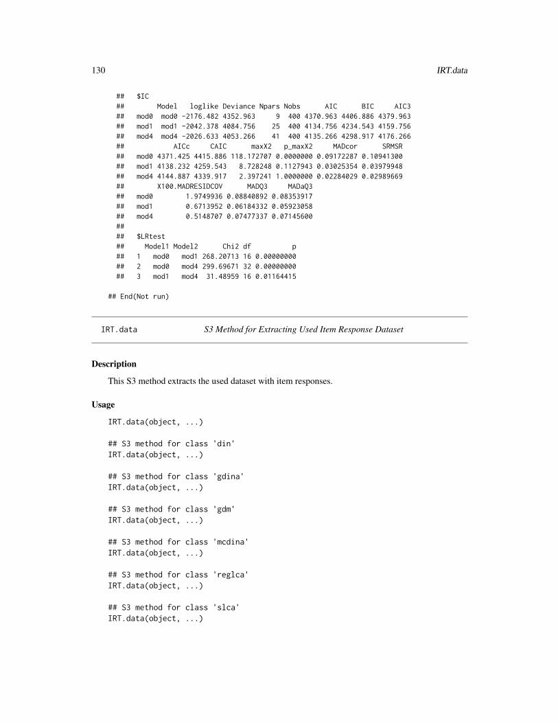
130 IRT.data

## $IC## Model loglike Deviance Npars Nobs AIC BIC AIC3## mod0 mod0 -2176.482 4352.963 9 400 4370.963 4406.886 4379.963## mod1 mod1 -2042.378 4084.756 25 400 4134.756 4234.543 4159.756## mod4 mod4 -2026.633 4053.266 41 400 4135.266 4298.917 4176.266## AICc CAIC maxX2 p_maxX2 MADcor SRMSR## mod0 4371.425 4415.886 118.172707 0.0000000 0.09172287 0.10941300## mod1 4138.232 4259.543 8.728248 0.1127943 0.03025354 0.03979948## mod4 4144.887 4339.917 2.397241 1.0000000 0.02284029 0.02989669## X100.MADRESIDCOV MADQ3 MADaQ3## mod0 1.9749936 0.08840892 0.08353917## mod1 0.6713952 0.06184332 0.05923058## mod4 0.5148707 0.07477337 0.07145600#### $LRtest## Model1 Model2 Chi2 df p## 1 mod0 mod1 268.20713 16 0.00000000## 2 mod0 mod4 299.69671 32 0.00000000## 3 mod1 mod4 31.48959 16 0.01164415

## End(Not run)

IRT.data S3 Method for Extracting Used Item Response Dataset

Description

This S3 method extracts the used dataset with item responses.

Usage

IRT.data(object, ...)

## S3 method for class 'din'IRT.data(object, ...)

## S3 method for class 'gdina'IRT.data(object, ...)

## S3 method for class 'gdm'IRT.data(object, ...)

## S3 method for class 'mcdina'IRT.data(object, ...)

## S3 method for class 'reglca'IRT.data(object, ...)

## S3 method for class 'slca'IRT.data(object, ...)

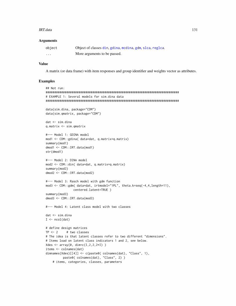
IRT.data 131

Arguments

object Object of classes din, gdina, mcdina, gdm, slca, reglca.

... More arguments to be passed.

Value

A matrix (or data frame) with item responses and group identifier and weights vector as attributes.

Examples

## Not run:############################################################################## EXAMPLE 1: Several models for sim.dina data#############################################################################



#--- Model 1: GDINA modelmod1 <- CDM::gdina( data=dat, q.matrix=q.matrix)summary(mod1)dmod1 <- CDM::IRT.data(mod1)str(dmod1)

#--- Model 2: DINA modelmod2 <- CDM::din( data=dat, q.matrix=q.matrix)summary(mod2)dmod2 <- CDM::IRT.data(mod2)

#--- Model 3: Rasch model with gdm functionmod3 <- CDM::gdm( data=dat, irtmodel="1PL", theta.k=seq(-4,4,length=11),

centered.latent=TRUE )summary(mod3)dmod3 <- CDM::IRT.data(mod3)

#--- Model 4: Latent class model with two classes

dat <- sim.dinaI <- ncol(dat)

# define design matricesTP <- 2 # two classes# The idea is that latent classes refer to two different "dimensions".# Items load on latent class indicators 1 and 2, see below.Xdes <- array(0, dim=c(I,2,2,2*I) )items <- colnames(dat)dimnames(Xdes)[[4]] <- c(paste0( colnames(dat), "Class", 1),

paste0( colnames(dat), "Class", 2) )# items, categories, classes, parameters

132 IRT.expectedCounts

# probabilities for correct solutionfor (ii in 1:I){

Xdes[ ii, 2, 1, ii ] <- 1 # probabilities class 1Xdes[ ii, 2, 2, ii+I ] <- 1 # probabilities class 2

}# estimate modelmod4 <- CDM::slca( dat, Xdes=Xdes)summary(mod4)dmod4 <- CDM::IRT.data(mod4)

## End(Not run)

IRT.expectedCounts S3 Method for Extracting Expected Counts

Description

This S3 method extracts expected counts from model output.

Usage

IRT.expectedCounts(object, ...)

## S3 method for class 'din'IRT.expectedCounts(object, ...)

## S3 method for class 'gdina'IRT.expectedCounts(object, ...)

## S3 method for class 'gdm'IRT.expectedCounts(object, ...)

## S3 method for class 'mcdina'IRT.expectedCounts(object, ...)

## S3 method for class 'slca'IRT.expectedCounts(object, ...)

## S3 method for class 'reglca'IRT.expectedCounts(object, ...)

Arguments

object Object of classes din, gdina, mcdina, gdm or slca.... More arguments to be passed.

Value

An array with expected counts. The dimensions are items, categories, latent classes and groups.

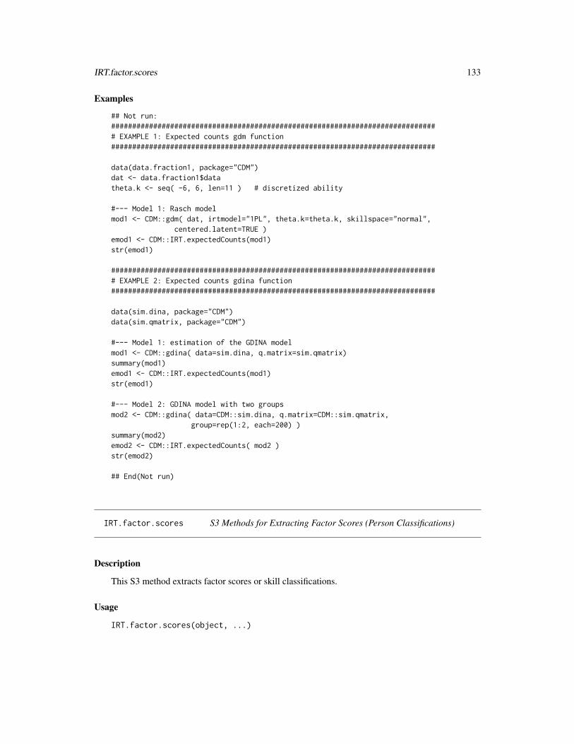
IRT.factor.scores 133

Examples

## Not run:############################################################################## EXAMPLE 1: Expected counts gdm function#############################################################################

data(data.fraction1, package="CDM")dat <- data.fraction1$datatheta.k <- seq( -6, 6, len=11 ) # discretized ability

#--- Model 1: Rasch modelmod1 <- CDM::gdm( dat, irtmodel="1PL", theta.k=theta.k, skillspace="normal",

centered.latent=TRUE )emod1 <- CDM::IRT.expectedCounts(mod1)str(emod1)

############################################################################## EXAMPLE 2: Expected counts gdina function#############################################################################


#--- Model 1: estimation of the GDINA modelmod1 <- CDM::gdina( data=sim.dina, q.matrix=sim.qmatrix)summary(mod1)emod1 <- CDM::IRT.expectedCounts(mod1)str(emod1)

#--- Model 2: GDINA model with two groupsmod2 <- CDM::gdina( data=CDM::sim.dina, q.matrix=CDM::sim.qmatrix,

group=rep(1:2, each=200) )summary(mod2)emod2 <- CDM::IRT.expectedCounts( mod2 )str(emod2)

## End(Not run)

IRT.factor.scores S3 Methods for Extracting Factor Scores (Person Classifications)

Description

This S3 method extracts factor scores or skill classifications.

Usage

IRT.factor.scores(object, ...)

134 IRT.factor.scores

## S3 method for class 'din'IRT.factor.scores(object, type="MLE", ...)

## S3 method for class 'gdina'IRT.factor.scores(object, type="MLE", ...)

## S3 method for class 'mcdina'IRT.factor.scores(object, type="MLE", ...)

## S3 method for class 'gdm'IRT.factor.scores(object, type="EAP", ...)

## S3 method for class 'slca'IRT.factor.scores(object, type="MLE", ...)

Arguments

object Object of classes din, gdina, mcdina, gdm or slca.type Type of estimated factor score. This can be "MLE", "MAP" or "EAP". The type

EAP cannot be used for objects of class slca.... More arguments to be passed.

Value

A matrix or a vector with classified scores.

See Also

For extracting the individual likelihood or the individual posterior see IRT.likelihood or IRT.posterior.

Examples

############################################################################## EXAMPLE 1: Extracting factor scores in the DINA model#############################################################################


# estimate DINA modelmod1 <- CDM::din( sim.dina, q.matrix=sim.qmatrix)summary(mod1)# MLEfsc1a <- CDM::IRT.factor.scores(mod1)# MAPfsc1b <- CDM::IRT.factor.scores(mod1, type="MAP")# EAPfsc1c <- CDM::IRT.factor.scores(mod1, type="EAP")# compare classification for skill 1stats::xtabs( ~ fsc1a[,1] + fsc1b[,1] )graphics::boxplot( fsc1c[,1] ~ fsc1a[,1] )

IRT.frequencies 135

IRT.frequencies S3 Method for Computing Observed and Expected Frequencies of Uni-variate and Bivariate Marginals

Description

This S3 method computes observed and expected frequencies for univariate and bivariate distribu-tions.

Usage

IRT.frequencies(object, ...)

IRT_frequencies_default(data, post, probs, weights=NULL)

IRT_frequencies_wrapper(object, ...)

## S3 method for class 'din'IRT.frequencies(object, ...)

## S3 method for class 'gdina'IRT.frequencies(object, ...)

## S3 method for class 'mcdina'IRT.frequencies(object, ...)

## S3 method for class 'gdm'IRT.frequencies(object, ...)

## S3 method for class 'slca'IRT.frequencies(object, ...)

Arguments

object Object of classes din, gdina, mcdina, gdm or slca.


data Item response data as extracted by IRT.data

post Individual posterior distribution as extracted by IRT.posterior

probs Individual posterior distribution as extracted by IRT.irfprob

weights Optional vector of weights as included as the attribute weights in IRT.data

Value

List with following entries

uni_obs Univariate observed distribution

136 IRT.IC

uni_exp Univariate expected distribution

M_obs Univariate observed means

M_exp Univariate expected means

SD_obs Univariate observed standard deviations

SD_exp Univariate expected standard deviations

biv_obs Bivariate observed frequencies

biv_exp Bivariate expected frequencies

biv_N Bivariate sample size

cov_obs Observed covariances

cov_cor Expected covariances

cor_obs Observed correlations

cor_exp Expected correlations

chisq Chi square statistic of local independence

Examples

## Not run:############################################################################## EXAMPLE 1: Usage IRT.frequencies#############################################################################


# estimate GDINA modelmod1 <- CDM::gdina( data=sim.dina, q.matrix=sim.qmatrix)summary(mod1)

# direct usage of IRT.frequenciesfres1 <- CDM::IRT.frequencies(mod1)

# use of the default function with input datadata <- CDM::IRT.data(object)post <- CDM::IRT.posterior(object)probs <- CDM::IRT.irfprob(object)fres2 <- CDM::IRT_frequencies_default(data=data, post=post, probs=probs)

## End(Not run)

IRT.IC Information Criteria

Description

Computes several information criteria for objects which do have the logLik (stats) S3 method (e.g.din, gdina, gdm, ...) .

IRT.irfprob 137

Usage

IRT.IC(object)

Arguments

object Objects which do have the logLik (stats) S3 method.

Value

A vector with deviance and several information criteria.

See Also

See also anova.din for model comparisons. A general method is defined in IRT.compareModels.

Examples

############################################################################## EXAMPLE 1: DINA example information criteria#############################################################################


#*** Model 1: DINA modelmod1 <- CDM::din( sim.dina, q.matrix=sim.qmatrix )summary(mod1)IRT.IC(mod1)

IRT.irfprob S3 Methods for Extracting Item Response Functions

Description

This S3 method extracts item response functions evaluated at a grid of abilities (skills). Item re-sponse functions can be plotted using the IRT.irfprobPlot function.

Usage

IRT.irfprob(object, ...)

## S3 method for class 'din'IRT.irfprob(object, ...)

## S3 method for class 'gdina'IRT.irfprob(object, ...)

## S3 method for class 'gdm'

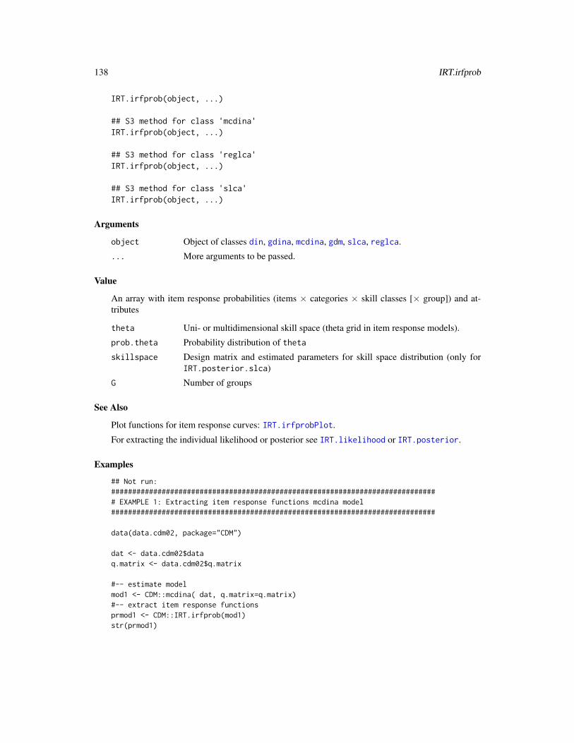
138 IRT.irfprob

IRT.irfprob(object, ...)

## S3 method for class 'mcdina'IRT.irfprob(object, ...)

## S3 method for class 'reglca'IRT.irfprob(object, ...)

## S3 method for class 'slca'IRT.irfprob(object, ...)

Arguments



Value

An array with item response probabilities (items × categories × skill classes [× group]) and at-tributes

theta Uni- or multidimensional skill space (theta grid in item response models).

prob.theta Probability distribution of theta

skillspace Design matrix and estimated parameters for skill space distribution (only forIRT.posterior.slca)

G Number of groups

See Also

Plot functions for item response curves: IRT.irfprobPlot.

For extracting the individual likelihood or posterior see IRT.likelihood or IRT.posterior.

Examples

## Not run:############################################################################## EXAMPLE 1: Extracting item response functions mcdina model#############################################################################


dat <- data.cdm02$dataq.matrix <- data.cdm02$q.matrix

#-- estimate modelmod1 <- CDM::mcdina( dat, q.matrix=q.matrix)#-- extract item response functionsprmod1 <- CDM::IRT.irfprob(mod1)str(prmod1)

IRT.irfprobPlot 139

## End(Not run)

IRT.irfprobPlot Plot Item Response Functions

Description

This function plots item response functions for fitted item response models for which the IRT.irfprobmethod is defined.

Usage

IRT.irfprobPlot( object, items=NULL, min.theta=-4, max.theta=4, cumul=FALSE,smooth=TRUE, ask=TRUE, n.theta=40, package="lattice",... )

Arguments

object Fitted item response model for which the IRT.irfprob method is defined

items Vector of indices of selected items.

min.theta Minimum theta to be displayed.

max.theta Maximum theta to be displayed.

cumul Optional logical indicating whether cumulated item response functions P (X ≥k|θ) should be displayed.

smooth Optional logical indicating whether item response functions should be smoothedfor plotting.

ask Logical for asking for a new plot.

n.theta Number of theta points if smooth=TRUE is chosen.

package String indicating which package should be used for plotting the item responsecurves. Options are "lattice" or "graphics".

... More arguments to be passed for the plot in lattice.

Examples

## Not run:############################################################################## EXAMPLE 1: Plot item response functions from a unidimensional model#############################################################################

data(data.Students, package="CDM")

dat <- data.Studentsresp <- dat[, paste0("sc",1:4) ]resp[ paste(resp[,1])==3,1] <- 2psych::describe(resp)

#--- Model 1: PCM in CDM::gdm

140 IRT.itemfit

theta.k <- seq( -5, 5, len=21 )mod1 <- CDM::gdm( dat=resp, irtmodel="1PL", theta.k=theta.k, skillspace="normal",

centered.latent=TRUE)summary(mod1)

# plotIRT.irfprobPlot( mod1 )# plot in graphics package (which comes with R base version)IRT.irfprobPlot( mod1, package="graphics")# plot first and third item and do not smooth discretized item response# functions in IRT.irfprobIRT.irfprobPlot( mod1, items=c(1,3), smooth=FALSE )# cumulated IRFIRT.irfprobPlot( mod1, cumul=TRUE )

############################################################################## EXAMPLE 2: Fitted mutidimensional model with gdm#############################################################################

dat <- CDM::data.fraction2$dataQmatrix <- CDM::data.fraction2$q.matrix3

# Model 1: 3-dimensional Rasch Model (normal distribution)theta.k <- seq( -4, 4, len=11 ) # discretized abilitymod1 <- CDM::gdm( dat, irtmodel="1PL", theta.k=theta.k, Qmatrix=Qmatrix,

centered.latent=TRUE, maxiter=10 )summary(mod1)

# unsmoothed curvesIRT.irfprobPlot(mod1, smooth=FALSE)# smoothed curvesIRT.irfprobPlot(mod1)

## End(Not run)

IRT.itemfit S3 Methods for Computing Item Fit

Description

This S3 method computes some selected item fit statistic.

Usage

IRT.itemfit(object, ...)

## S3 method for class 'din'IRT.itemfit(object, method="RMSEA", ...)

## S3 method for class 'gdina'

IRT.itemfit 141

IRT.itemfit(object, method="RMSEA", ...)

## S3 method for class 'gdm'IRT.itemfit(object, method="RMSEA", ...)

## S3 method for class 'reglca'IRT.itemfit(object, method="RMSEA", ...)

## S3 method for class 'slca'IRT.itemfit(object, method="RMSEA", ...)

Arguments

object Object of classes din, gdina, gdm, slca, reglca.

method Method for computing item fit statistic. Until now, only method="RMSEA" (seeitemfit.rmsea) can be used.


Value

Vector or data frame with item fit statistics.

See Also


Examples

## Not run:############################################################################## EXAMPLE 1: DINA model item fit#############################################################################


# estimate modelmod1 <- CDM::din( sim.dina, q.matrix=sim.qmatrix)# compute item fitIRT.itemfit( mod1 )

## End(Not run)

142 IRT.jackknife

IRT.jackknife Jackknifing an Item Response Model

Description

This function performs a Jackknife procedure for estimating standard errors for an item responsemodel. The replication design must be defined by IRT.repDesign. Model fit is also assessed viaJackknife.

Statistical inference for derived parameters is performed by IRT.derivedParameters with a fittedobject of class IRT.jackknife and a list with defining formulas.

Usage

IRT.jackknife(object,repDesign, ... )

IRT.derivedParameters(jkobject, derived.parameters )

## S3 method for class 'gdina'IRT.jackknife(object, repDesign, ...)

## S3 method for class 'IRT.jackknife'coef(object, bias.corr=FALSE, ...)

## S3 method for class 'IRT.jackknife'vcov(object, ...)

Arguments

object Objects for which S3 method IRT.jackknife is defined.

repDesign Replication design generated by IRT.repDesign.

jkobject Object of class IRT.jackknife.derived.parameters

List with defined derived parameters (see Example 2, Model 2).

bias.corr Optional logical indicating whether a bias correction should be employed.

... Further arguments to be passed.

Value


jpartable Parameter table with Jackknife estimates

parsM Matrix with replicated statistics

vcov Variance covariance matrix of parameters

IRT.jackknife 143

Examples

## Not run:library(BIFIEsurvey)

############################################################################## EXAMPLE 1: Multiple group DINA model with TIMSS data | Cluster sample#############################################################################

data(data.timss11.G4.AUT.part, package="CDM")

dat <- data.timss11.G4.AUT.part$dataq.matrix <- data.timss11.G4.AUT.part$q.matrix2# extract itemsitems <- paste(q.matrix$item)

# generate replicate designrdes <- CDM::IRT.repDesign( data=dat, wgt="TOTWGT", jktype="JK_TIMSS",

jkzone="JKCZONE", jkrep="JKCREP" )

#--- Model 1: fit multiple group GDINA modelmod1 <- CDM::gdina( dat[,items], q.matrix=q.matrix[,-1],

weights=dat$TOTWGT, group=dat$female +1 )# jackknife Model 1jmod1 <- CDM::IRT.jackknife( object=mod1, repDesign=rdes )summary(jmod1)coef(jmod1)vcov(jmod1)

############################################################################## EXAMPLE 2: DINA model | Simple random sampling#############################################################################

data(sim.dina, package="CDM")data(sim.qmatrix, package="CDM")dat <- sim.dinaq.matrix <- sim.qmatrix

# generate replicate design with 50 jackknife zones (50 random groups)rdes <- CDM::IRT.repDesign( data=dat, jktype="JK_RANDOM", ngr=50 )

#--- Model 1: DINA modelmod1 <- CDM::gdina( dat, q.matrix=q.matrix, rule="DINA")summary(mod1)# jackknife DINA modeljmod1 <- CDM::IRT.jackknife( object=mod1, repDesign=rdes )summary(jmod1)

#--- Model 2: DINO modelmod2 <- CDM::gdina( dat, q.matrix=q.matrix, rule="DINO")summary(mod2)# jackknife DINA modeljmod2 <- CDM::IRT.jackknife( object=mod2, repDesign=rdes )

144 IRT.likelihood

summary(jmod2)IRT.compareModels( mod1, mod2 )

# statistical inference for derived parametersderived.parameters <- list( "skill1"=~ 0 + I(prob_skillV1_lev1_group1),

"skilldiff12"=~ 0 + I( prob_skillV2_lev1_group1 - prob_skillV1_lev1_group1 ),"skilldiff13"=~ 0 + I( prob_skillV3_lev1_group1 - prob_skillV1_lev1_group1 )

)jmod2a <- CDM::IRT.derivedParameters( jmod2, derived.parameters=derived.parameters )summary(jmod2a)coef(jmod2a)

## End(Not run)

IRT.likelihood S3 Methods for Extracting of the Individual Likelihood and the Indi-vidual Posterior

Description

Functions for extracting the individual likelihood and individual posterior distribution.

Usage

IRT.likelihood(object, ...)

IRT.posterior(object, ...)

## S3 method for class 'din'IRT.likelihood(object, ...)## S3 method for class 'din'IRT.posterior(object, ...)

## S3 method for class 'gdina'IRT.likelihood(object, ...)## S3 method for class 'gdina'IRT.posterior(object, ...)

## S3 method for class 'gdm'IRT.likelihood(object, ...)## S3 method for class 'gdm'IRT.posterior(object, ...)

## S3 method for class 'mcdina'IRT.likelihood(object, ...)## S3 method for class 'mcdina'IRT.posterior(object, ...)

IRT.likelihood 145

## S3 method for class 'reglca'IRT.likelihood(object, ...)## S3 method for class 'reglca'IRT.posterior(object, ...)

## S3 method for class 'slca'IRT.likelihood(object, ...)## S3 method for class 'slca'IRT.posterior(object, ...)

Arguments



Value

For both functions IRT.likelihood and IRT.posterior, it is a matrix with attributes

theta Uni- or multidimensional skill space (theta grid in item response models).

prob.theta Probability distribution of theta

skillspace Design matrix and estimated parameters for skill space distribution (only forIRT.posterior.slca)

G Number of groups

See Also

GDINA::indlogLik, GDINA::indlogPost

Examples

############################################################################## EXAMPLE 1: Extracting likelihood and posterior from a DINA model#############################################################################


#*** estimate modelmod1 <- CDM::din( sim.dina, q.matrix=sim.qmatrix, rule="DINA")#*** extract likelihoodlikemod1 <- CDM::IRT.likelihood(mod1)str(likemod1)# extract thetaattr(likemod1, "theta" )#*** extract posteriorpomod1 <- CDM::IRT.posterior( mod1 )str(pomod1)

146 IRT.marginal_posterior

IRT.marginal_posterior

S3 Method for Computation of Marginal Posterior Distribution

Description

Computes marginal posterior distributions for fitted models in the CDM package.

Usage

IRT.marginal_posterior(object, dim, remove_zeroprobs=TRUE, ...)

## S3 method for class 'din'IRT.marginal_posterior(object, dim, remove_zeroprobs=TRUE, ...)## S3 method for class 'gdina'IRT.marginal_posterior(object, dim, remove_zeroprobs=TRUE, ...)## S3 method for class 'mcdina'IRT.marginal_posterior(object, dim, remove_zeroprobs=TRUE, ...)

Arguments

object Object of class din, gdina, mcdina

dim Numeric or character vector indicating dimensions of posterior distribution whichshould be marginalized

remove_zeroprobs

Logical indicating whether classes with zero probabilities should be removed


Value

List with entries

marg_post Marginal posterior distribution

map MAP estimate (individual classification)

theta Skill classes

See Also

IRT.posterior

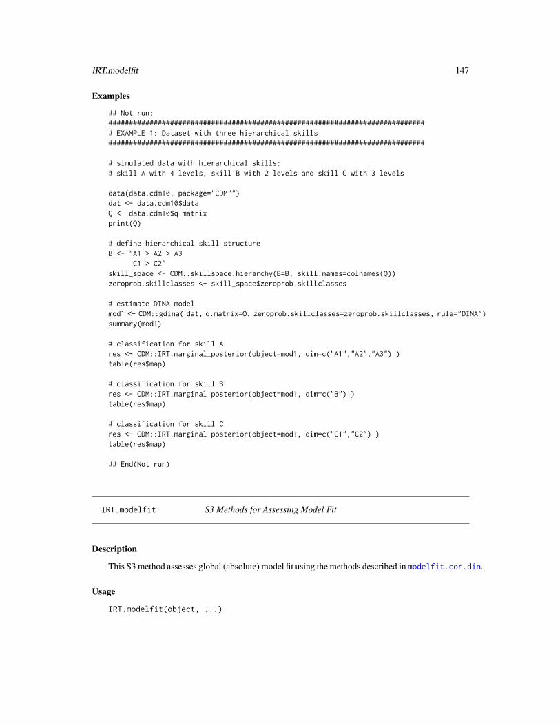
IRT.modelfit 147

Examples

## Not run:############################################################################## EXAMPLE 1: Dataset with three hierarchical skills#############################################################################

# simulated data with hierarchical skills:# skill A with 4 levels, skill B with 2 levels and skill C with 3 levels

data(data.cdm10, package="CDM"")dat <- data.cdm10$dataQ <- data.cdm10$q.matrixprint(Q)

# define hierarchical skill structureB <- "A1 > A2 > A3

C1 > C2"skill_space <- CDM::skillspace.hierarchy(B=B, skill.names=colnames(Q))zeroprob.skillclasses <- skill_space$zeroprob.skillclasses

# estimate DINA modelmod1 <- CDM::gdina( dat, q.matrix=Q, zeroprob.skillclasses=zeroprob.skillclasses, rule="DINA")summary(mod1)

# classification for skill Ares <- CDM::IRT.marginal_posterior(object=mod1, dim=c("A1","A2","A3") )table(res$map)

# classification for skill Bres <- CDM::IRT.marginal_posterior(object=mod1, dim=c("B") )table(res$map)

# classification for skill Cres <- CDM::IRT.marginal_posterior(object=mod1, dim=c("C1","C2") )table(res$map)

## End(Not run)

IRT.modelfit S3 Methods for Assessing Model Fit

Description

This S3 method assesses global (absolute) model fit using the methods described in modelfit.cor.din.

Usage

IRT.modelfit(object, ...)

148 IRT.modelfit

## S3 method for class 'din'IRT.modelfit(object, ...)## S3 method for class 'gdina'IRT.modelfit(object, ...)

## S3 method for class 'IRT.modelfit.din'summary(object, ...)## S3 method for class 'IRT.modelfit.gdina'summary(object, ...)

Arguments

object Object of classes din or gdina.


Value

See output of modelfit.cor.din.

See Also


The model fit of objects of class gdm can be obtained by using the TAM::tam.modelfit.IRT func-tion in the TAM package.

Examples

## Not run:############################################################################## EXAMPLE 1: Absolute model fit#############################################################################


#*** Model 1: DINA model for DINA simulated datamod1 <- CDM::din( sim.dina, q.matrix=sim.qmatrix, rule="DINA" )fmod1 <- CDM::IRT.modelfit( mod1 )summary(fmod1)

## Test of Global Model Fit## type value p## 1 max(X2) 8.728 0.113## 2 abs(fcor) 0.143 0.080#### Fit Statistics## est## MADcor 0.030## SRMSR 0.040## 100*MADRESIDCOV 0.671## MADQ3 0.062## MADaQ3 0.059

IRT.parameterTable 149

#*** Model 2: GDINA modelmod2 <- CDM::gdina( sim.dina, q.matrix=sim.qmatrix, rule="GDINA" )fmod2 <- CDM::IRT.modelfit( mod2 )summary(fmod2)

## Test of Global Model Fit## type value p## 1 max(X2) 2.397 1## 2 abs(fcor) 0.078 1#### Fit Statistics## est## MADcor 0.023## SRMSR 0.030## 100*MADRESIDCOV 0.515## MADQ3 0.075## MADaQ3 0.071

## End(Not run)

IRT.parameterTable S3 Method for Extracting a Parameter Table

Description

S3 method which extracts a parameter table.

Usage

IRT.parameterTable(object, ...)

Arguments

object Object of model classes


Value

A parameter table

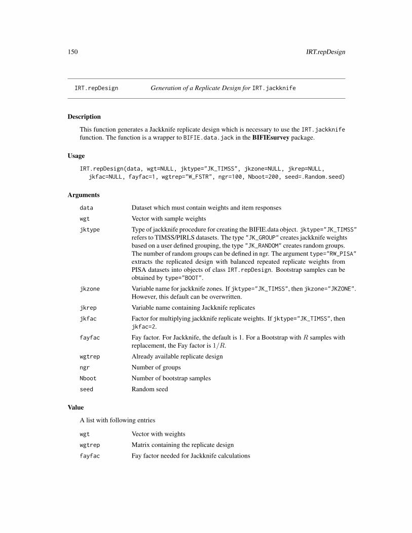
150 IRT.repDesign

IRT.repDesign Generation of a Replicate Design for IRT.jackknife

Description

This function generates a Jackknife replicate design which is necessary to use the IRT.jackknifefunction. The function is a wrapper to BIFIE.data.jack in the BIFIEsurvey package.

Usage

IRT.repDesign(data, wgt=NULL, jktype="JK_TIMSS", jkzone=NULL, jkrep=NULL,jkfac=NULL, fayfac=1, wgtrep="W_FSTR", ngr=100, Nboot=200, seed=.Random.seed)

Arguments

data Dataset which must contain weights and item responses

wgt Vector with sample weights

jktype Type of jackknife procedure for creating the BIFIE.data object. jktype="JK_TIMSS"refers to TIMSS/PIRLS datasets. The type "JK_GROUP" creates jackknife weightsbased on a user defined grouping, the type "JK_RANDOM" creates random groups.The number of random groups can be defined in ngr. The argument type="RW_PISA"extracts the replicated design with balanced repeated replicate weights fromPISA datasets into objects of class IRT.repDesign. Bootstrap samples can beobtained by type="BOOT".

jkzone Variable name for jackknife zones. If jktype="JK_TIMSS", then jkzone="JKZONE".However, this default can be overwritten.

jkrep Variable name containing Jackknife replicates

jkfac Factor for multiplying jackknife replicate weights. If jktype="JK_TIMSS", thenjkfac=2.

fayfac Fay factor. For Jackknife, the default is 1. For a Bootstrap with R samples withreplacement, the Fay factor is 1/R.

wgtrep Already available replicate design

ngr Number of groups

Nboot Number of bootstrap samples

seed Random seed

Value


wgt Vector with weights

wgtrep Matrix containing the replicate design

fayfac Fay factor needed for Jackknife calculations

IRT.RMSD 151

See Also

See IRT.jackknife for further examples.

See the BIFIE.data.jack function in the BIFIEsurvey package.

Examples

## Not run:# load the BIFIEsurvey packagelibrary(BIFIEsurvey)

############################################################################## EXAMPLE 1: Design with Jackknife replicate weights in TIMSS#############################################################################

data(data.timss11.G4.AUT, package="CDM")dat <- CDM::data.timss11.G4.AUT$data# generate designrdes <- CDM::IRT.repDesign( data=dat, wgt="TOTWGT", jktype="JK_TIMSS",

jkzone="JKCZONE", jkrep="JKCREP" )str(rdes)

############################################################################## EXAMPLE 2: Bootstrap resampling#############################################################################

data(sim.qmatrix, package="CDM")q.matrix <- CDM::sim.qmatrix

# simulate data according to the DINA modeldat <- CDM::sim.din(N=2000, q.matrix=q.matrix )$dat

# bootstrap with 300 random samplesrdes <- CDM::IRT.repDesign( data=dat, jktype="BOOT", Nboot=300 )

## End(Not run)

IRT.RMSD Root Mean Square Deviation (RMSD) Item Fit Statistic

Description

Computed the item fit statistics root mean square deviation (RMSD), mean absolute deviation(MAD) and mean deviation (MD). See Oliveri and von Davier (2011) for details.

The RMSD statistics was denoted as the RMSEA statistic in older publications, see itemfit.rmsea.

If multiple groups are defined in the model object, a weighted item fit statistic (WRMSD; Ya-mamoto, Khorramdel, & von Davier, 2013; von Davier, Weeks, Chen, Allen & van der Velden,2013) is additionally computed.

152 IRT.RMSD

Usage

IRT.RMSD(object)

## S3 method for class 'IRT.RMSD'summary(object, file=NULL, digits=3, ...)

## core computation functionIRT_RMSD_calc_rmsd( n.ik, pi.k, probs, eps=1E-30 )

Arguments

object Object for which the methods IRT.expectedCounts and IRT.irfprob can beapplied.

n.ik Expected counts

pi.k Probabilities trait distribution

probs Item response probabilities

eps Numerical constant avoiding division by zero

digits Number of digits used for rounding


... Optional parameters to be passed.

Details

The RMSD and MD statistics are in operational use in PISA studies since PISA 2015. These fitstatistics can also be used for investigating uniform and nonuniform differential item functioning.

Value

List with entries

RMSD Item-wise and group-wise RMSD statistic

RMSD_bc Item-wise and group-wise RMSD statistic with analytical bias correction

MAD Item-wise and group-wise MAD statistic

MD Item-wise and group-wise MD statistic

chisquare_stat Item-wise and group-wise χ2 statistic

... Further values

References

Oliveri, M. E., & von Davier, M. (2011). Investigation of model fit and score scale comparabilityin international assessments. Psychological Test and Assessment Modeling, 53, 315-333.

von Davier, M., Weeks, J., Chen, H., Allen, J., & van der Velden, R. (2013). Creating simpleand complex derived variables and validation of background questionnaire data. In OECD (Eds.).Technical Report of the Survey of Adults Skills (PIAAC) (Ch. 20). Paris: OECD.

Yamamoto, K., Khorramdel, L., & von Davier, M. (2013). Scaling PIAAC cognitive data. In OECD(Eds.). Technical Report of the Survey of Adults Skills (PIAAC) (Ch. 17). Paris: OECD.

IRT.RMSD 153

See Also

itemfit.rmsea

Examples

## Not run:############################################################################## EXAMPLE 1: data.read | 1PL model in TAM#############################################################################

data(data.read, package="sirt")dat <- data.read

#*** Model 1: 1PL modelmod1 <- TAM::tam.mml( resp=dat )summary(mod1)

# item fit statisticsimod1 <- CDM::IRT.RMSD(mod1)summary(imod1)

############################################################################## EXAMPLE 2: data.math| RMSD and MD statistic for assessing DIF#############################################################################

data(data.math, package="sirt")dat <- data.math$dataitems <- grep("M[A-Z]", colnames(dat), value=TRUE )

#-- fit multiple group Rasch modelmod <- TAM::tam.mml( dat[,items], group=dat$female )summary(mod)

#-- fit statisticsrmod <- CDM::IRT.RMSD(mod)summary(rmod)

############################################################################## EXAMPLE 3: RMSD statistic DINA model#############################################################################

data(sim.dina)data(sim.qmatrix)dat <- sim.dinaQ <- sim.qmatrix

#-- fit DINA modelmod1 <- CDM::gdina( dat, q.matrix=Q, rule="DINA" )summary(mod1)

#-- compute RMSD fit statisticrmod1 <- CDM::IRT.RMSD(mod1)

154 itemfit.rmsea

summary(rmod1)

## End(Not run)

itemfit.rmsea RMSEA Item Fit

Description

This function estimates a chi squared based measure of item fit in cognitive diagnosis models similarto the RMSEA itemfit implemented in mdltm (von Davier, 2005; cited in Kunina-Habenicht, Rupp& Wilhelm, 2009).

The RMSEA statistic is also called as the RMSD statistic, see IRT.RMSD.

Usage

itemfit.rmsea(n.ik, pi.k, probs, itemnames=NULL)

Arguments

n.ik An array of four dimensions: Classes x items x categories x groups

pi.k An array of two dimensions: Classes x groups

probs An array of three dimensions: Classes x items x categories

itemnames An optional vector of item names. Default is NULL.

Details

For item j, the RMSEA itemfit in this function is calculated as follows:

RMSEAj =

√√√√∑k

∑c

π(θc)

(Pj(θc)−

njkcNjc

)2

where c denotes the class of the skill vector θ, k is the item category, π(θc) is the estimated classprobability of θc, Pj is the estimated item response function, njkc is the expected number of stu-dents with skill θc on item j in category k and Njc is the expected number of students with skill θcon item j.

Value

A list with two entries:

rmsea Vector of RMSEA item statistics

rmsea.groups Matrix of group-wise RMSEA item statistics

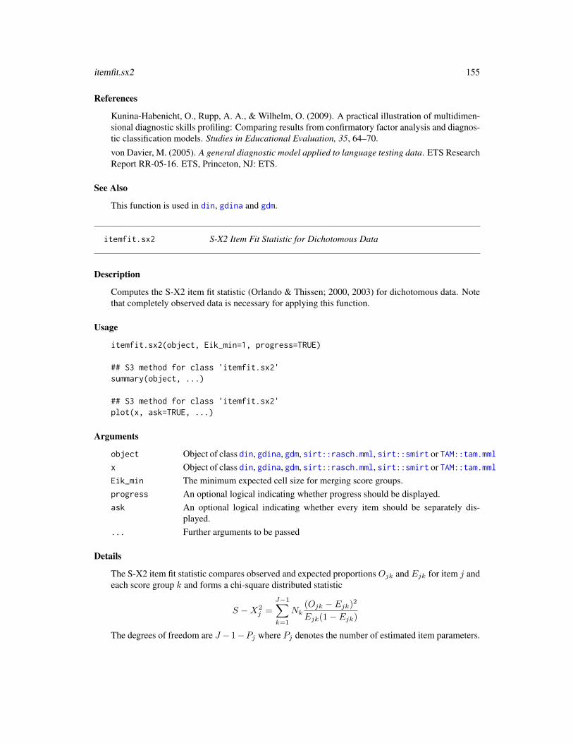
itemfit.sx2 155

References

Kunina-Habenicht, O., Rupp, A. A., & Wilhelm, O. (2009). A practical illustration of multidimen-sional diagnostic skills profiling: Comparing results from confirmatory factor analysis and diagnos-tic classification models. Studies in Educational Evaluation, 35, 64–70.

von Davier, M. (2005). A general diagnostic model applied to language testing data. ETS ResearchReport RR-05-16. ETS, Princeton, NJ: ETS.

See Also

This function is used in din, gdina and gdm.

itemfit.sx2 S-X2 Item Fit Statistic for Dichotomous Data

Description

Computes the S-X2 item fit statistic (Orlando & Thissen; 2000, 2003) for dichotomous data. Notethat completely observed data is necessary for applying this function.

Usage

itemfit.sx2(object, Eik_min=1, progress=TRUE)

## S3 method for class 'itemfit.sx2'summary(object, ...)

## S3 method for class 'itemfit.sx2'plot(x, ask=TRUE, ...)

Arguments

object Object of class din, gdina, gdm, sirt::rasch.mml, sirt::smirt or TAM::tam.mmlx Object of class din, gdina, gdm, sirt::rasch.mml, sirt::smirt or TAM::tam.mmlEik_min The minimum expected cell size for merging score groups.progress An optional logical indicating whether progress should be displayed.ask An optional logical indicating whether every item should be separately dis-

played.... Further arguments to be passed

Details

The S-X2 item fit statistic compares observed and expected proportions Ojk and Ejk for item j andeach score group k and forms a chi-square distributed statistic

S −X2j =

J−1∑k=1

Nk(Ojk − Ejk)2

Ejk(1− Ejk)

The degrees of freedom are J − 1−Pj where Pj denotes the number of estimated item parameters.

156 itemfit.sx2

Value


itemfit.stat Data frame containing item fit statistics

itemtable Data frame with expected and observed proportions for each score group andeach item. Beside the ordinary p value, an adjusted p value obtained by correc-tion due to multiple testing is provided (p.holm, see stats::p.adjust.

Note

This function does not work properly for multiple groups.

Author(s)

Alexander Robitzsch

References

Li, Y., & Rupp, A. A. (2011). Performance of the S-X2 statistic for full-information bifactor models.Educational and Psychological Measurement, 71, 986-1005.

Orlando, M., & Thissen, D. (2000). Likelihood-based item-fit indices for dichotomous item re-sponse theory models. Applied Psychological Measurement, 24, 50-64.

Orlando, M., & Thissen, D. (2003). Further investigation of the performance of S-X2: An item fitindex for use with dichotomous item response theory models. Applied Psychological Measurement,27, 289-298.

Zhang, B., & Stone, C. A. (2008). Evaluating item fit for multidimensional item response models.Educational and Psychological Measurement, 68, 181-196.

Examples

############################################################################## EXAMPLE 1: Items with unequal item slopes#############################################################################

# simulate dataset.seed(9871)I <- 11b <- seq( -1.5, 1.5, length=I)a <- rep(1,I)a[4] <- .4N <- 1000library(sirt)dat <- sirt::sim.raschtype( theta=stats::rnorm(N), b=b, fixed.a=a)

#*** 1PL model estimated with gdmmod1 <- CDM::gdm( dat, theta.k=seq(-6,6,len=21), irtmodel="1PL" )summary(mod1)# estimate item fit statisticfitmod1 <- CDM::itemfit.sx2(mod1)

itemfit.sx2 157

summary(fitmod1)## item itemindex S-X2 df p S-X2_df RMSEA Nscgr Npars p.holm## 1 I0001 1 4.173 9 0.900 0.464 0.000 10 1 1.000## 2 I0002 2 12.365 9 0.193 1.374 0.019 10 1 1.000## 3 I0003 3 6.158 9 0.724 0.684 0.000 10 1 1.000## 4 I0004 4 37.759 9 0.000 4.195 0.057 10 1 0.000## 5 I0005 5 12.307 9 0.197 1.367 0.019 10 1 1.000## 6 I0006 6 19.358 9 0.022 2.151 0.034 10 1 0.223## 7 I0007 7 14.610 9 0.102 1.623 0.025 10 1 0.818## 8 I0008 8 15.568 9 0.076 1.730 0.027 10 1 0.688## 9 I0009 9 8.471 9 0.487 0.941 0.000 10 1 1.000## 10 I0010 10 8.330 9 0.501 0.926 0.000 10 1 1.000## 11 I0011 11 12.351 9 0.194 1.372 0.019 10 1 1.000#### -- Average Item Fit Statistics --## S-X2=13.768 | S-X2_df=1.53

# -> 4th item does not fit to the 1PL model

# plot item fitplot(fitmod1)

## Not run:#*** 2PL model estimated with gdmmod2 <- CDM::gdm( dat, theta.k=seq(-6,6,len=21), irtmodel="2PL", maxiter=100 )summary(mod2)# estimate item fit statisticfitmod2 <- CDM::itemfit.sx2(mod2)summary(fitmod2)

## item itemindex S-X2 df p S-X2_df RMSEA Nscgr Npars p.holm## 1 I0001 1 4.083 8 0.850 0.510 0.000 10 2 1.000## 2 I0002 2 13.580 8 0.093 1.697 0.026 10 2 0.747## 3 I0003 3 6.236 8 0.621 0.780 0.000 10 2 1.000## 4 I0004 4 6.049 8 0.642 0.756 0.000 10 2 1.000## 5 I0005 5 12.792 8 0.119 1.599 0.024 10 2 0.834## 6 I0006 6 14.397 8 0.072 1.800 0.028 10 2 0.648## 7 I0007 7 15.046 8 0.058 1.881 0.030 10 2 0.639## [...]#### -- Average Item Fit Statistics --## S-X2=10.22 | S-X2_df=1.277

#*** 1PL model estimation in smirt (sirt package)Qmatrix <- matrix(1, nrow=I, ncol=1 )mod1a <- sirt::smirt( dat, Qmatrix=Qmatrix )summary(mod1a)# item fit statisticfitmod1a <- CDM::itemfit.sx2(mod1a)summary(fitmod1a)

#*** 2PL model estimation in smirt (sirt package)mod2a <- sirt::smirt( dat, Qmatrix=Qmatrix, est.a="2PL")summary(mod2a)# item fit statistic

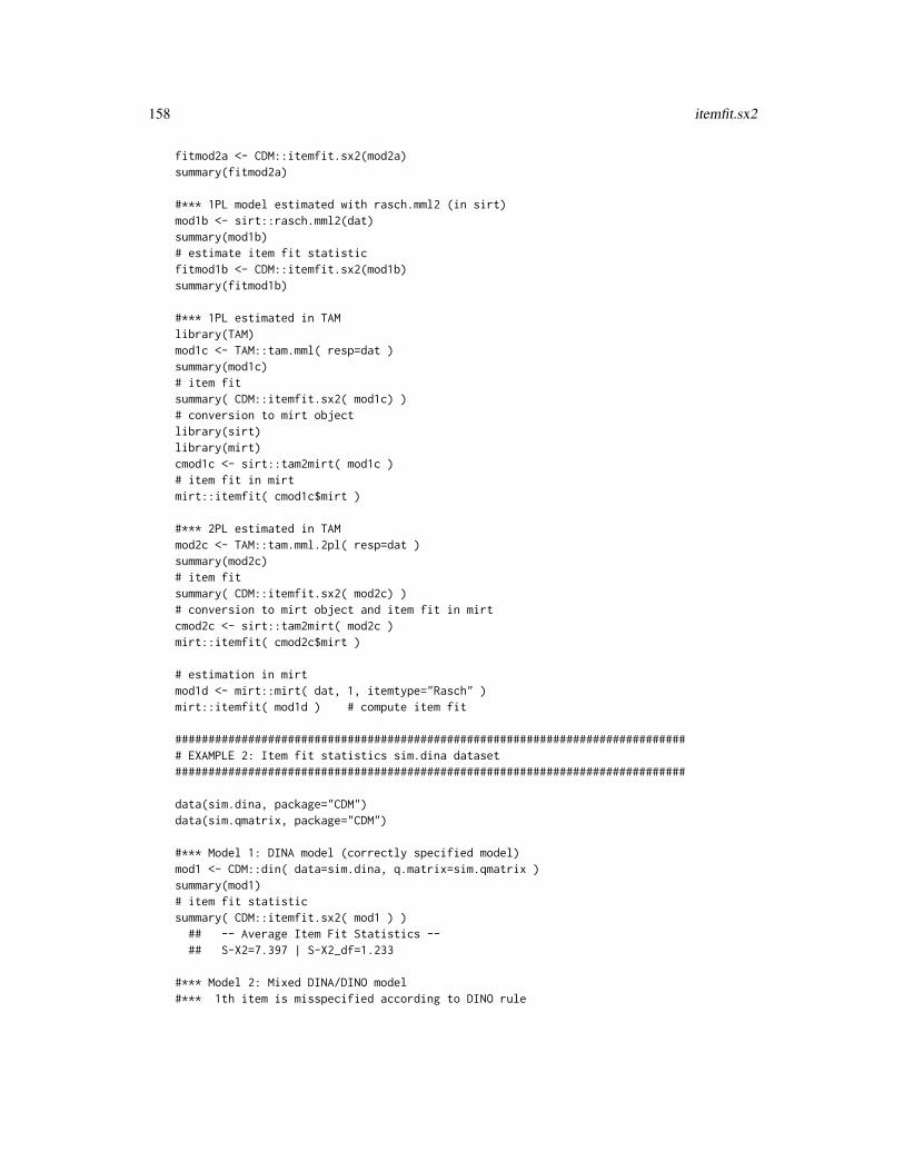
158 itemfit.sx2

fitmod2a <- CDM::itemfit.sx2(mod2a)summary(fitmod2a)

#*** 1PL model estimated with rasch.mml2 (in sirt)mod1b <- sirt::rasch.mml2(dat)summary(mod1b)# estimate item fit statisticfitmod1b <- CDM::itemfit.sx2(mod1b)summary(fitmod1b)

#*** 1PL estimated in TAMlibrary(TAM)mod1c <- TAM::tam.mml( resp=dat )summary(mod1c)# item fitsummary( CDM::itemfit.sx2( mod1c) )# conversion to mirt objectlibrary(sirt)library(mirt)cmod1c <- sirt::tam2mirt( mod1c )# item fit in mirtmirt::itemfit( cmod1c$mirt )

#*** 2PL estimated in TAMmod2c <- TAM::tam.mml.2pl( resp=dat )summary(mod2c)# item fitsummary( CDM::itemfit.sx2( mod2c) )# conversion to mirt object and item fit in mirtcmod2c <- sirt::tam2mirt( mod2c )mirt::itemfit( cmod2c$mirt )

# estimation in mirtmod1d <- mirt::mirt( dat, 1, itemtype="Rasch" )mirt::itemfit( mod1d ) # compute item fit

############################################################################## EXAMPLE 2: Item fit statistics sim.dina dataset#############################################################################


#*** Model 1: DINA model (correctly specified model)mod1 <- CDM::din( data=sim.dina, q.matrix=sim.qmatrix )summary(mod1)# item fit statisticsummary( CDM::itemfit.sx2( mod1 ) )

## -- Average Item Fit Statistics --## S-X2=7.397 | S-X2_df=1.233

#*** Model 2: Mixed DINA/DINO model#*** 1th item is misspecified according to DINO rule

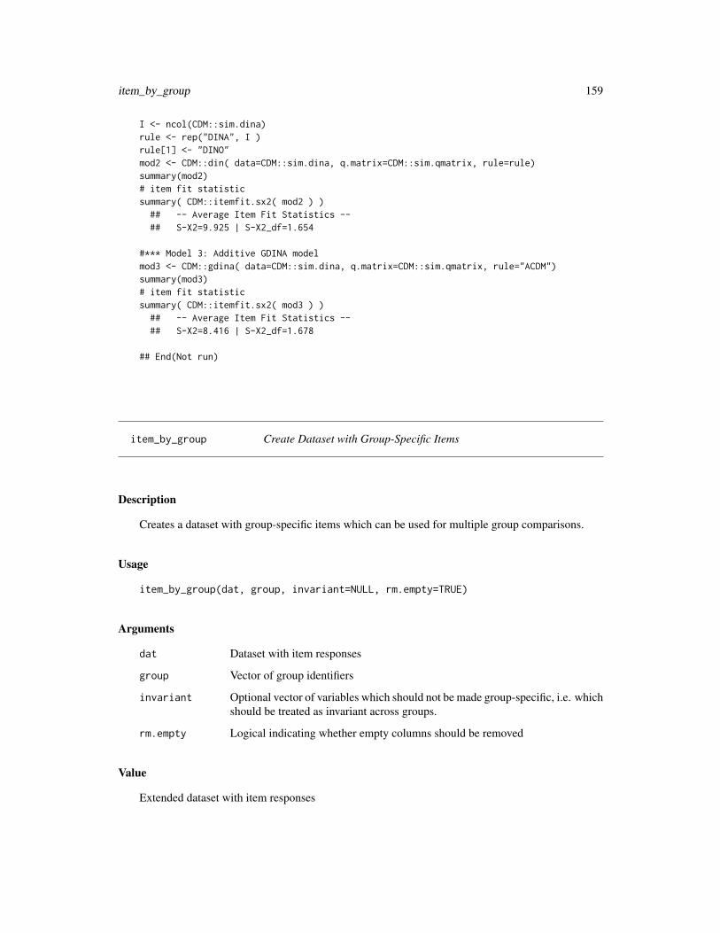
item_by_group 159

I <- ncol(CDM::sim.dina)rule <- rep("DINA", I )rule[1] <- "DINO"mod2 <- CDM::din( data=CDM::sim.dina, q.matrix=CDM::sim.qmatrix, rule=rule)summary(mod2)# item fit statisticsummary( CDM::itemfit.sx2( mod2 ) )


#*** Model 3: Additive GDINA modelmod3 <- CDM::gdina( data=CDM::sim.dina, q.matrix=CDM::sim.qmatrix, rule="ACDM")summary(mod3)# item fit statisticsummary( CDM::itemfit.sx2( mod3 ) )


## End(Not run)

item_by_group Create Dataset with Group-Specific Items

Description

Creates a dataset with group-specific items which can be used for multiple group comparisons.

Usage

item_by_group(dat, group, invariant=NULL, rm.empty=TRUE)

Arguments

dat Dataset with item responses

group Vector of group identifiers

invariant Optional vector of variables which should not be made group-specific, i.e. whichshould be treated as invariant across groups.

rm.empty Logical indicating whether empty columns should be removed

Value

Extended dataset with item responses

160 logLik

Examples

## Not run:############################################################################## EXAMPLE 1: Create dataset with group-specific item responses#############################################################################

data(data.mg, package="CDM")dat <- data.mg

#-- create dataset with group-specific item responsesdat0 <- CDM::item_by_group( dat=dat[,paste0("I",1:5)], group=dat$group )

#-- summary statisticssummary(dat0)colnames(dat0)

#-- set some items to invariantinvariant_items <- c("I1","I4")dat1 <- CDM::item_by_group( dat=dat[,paste0("I",1:5)], group=dat$group,

invariant=invariant_items)colnames(dat1)

## End(Not run)

logLik Extract Log-Likelihood

Description

Extracts the log-likelihood from either din, gdina, mcdina, slca or gdm objects.

Usage

## S3 method for class 'din'logLik(object, ...)

## S3 method for class 'gdina'logLik(object, ...)

## S3 method for class 'mcdina'logLik(object, ...)

## S3 method for class 'gdm'logLik(object, ...)

## S3 method for class 'slca'logLik(object, ...)

mcdina 161

## S3 method for class 'reglca'logLik(object, ...)

Arguments

object An object inheriting from either class din, gdina, slca, reglca or gdm.

... Additional arguments

See Also

din, gdina, gdm, mcdina, slca, reglca

Examples


# logLik method | DINA modeld1 <- CDM::din( sim.dina, q.matrix=sim.qmatrix, rule="DINA")summary(d1)lld1 <- logLik(d1)

## > lld1## 'log Lik.' -2042.378 (df=25)## > attr(lld1,"df")## [1] 25## > attr(lld1,"nobs")## [1] 400

nobs(lld1)

# AIC and BICAIC(lld1)BIC(lld1)

mcdina Multiple Choice DINA Model

Description

The function mcdina implements the multiple choice DINA model (de la Torre, 2009; see alsoOzaki, 2015; Chen & Zhou, 2017) for multiple groups. Note that the dataset must contain integervalues 1, . . . ,Kj for each item. The multiple choice DINA model assumes that each item categorypossesses different diagnostic capacity. Using this modeling approach, different distractors of amultiple choice item can be of different diagnostic value. The Q-matrix can also contain integervalues which allows the definition of polytomous attributes.

162 mcdina

Usage

mcdina(dat, q.matrix, group=NULL, itempars="gr", weights=NULL,skillclasses=NULL, zeroprob.skillclasses=NULL,reduced.skillspace=TRUE, conv.crit=1e-04,dev.crit=0.1, maxit=1000, progress=TRUE)

## S3 method for class 'mcdina'summary(object, digits=4, file=NULL, ...)

## S3 method for class 'mcdina'print(x, ...)

Arguments

dat A required N × J data matrix containing integer responses (1, 2, . . ., K) of Nrespondents to J test items.

q.matrix A required matrix specifying which item category is intended to measure whichskill. The Q-matrix has K + 2 columns for a model with K skills. In the firstcolumn should be the item index, in the second column the category integerand the rest of the columns contains the ’ordinary’ Q-matrix specification. Seedata.cdm01$q.matrix for the layout of such a Q-matrix.

group An optional vector of group identifiers for multiple group estimation.

itempars A character or a character vector of length J indicating whether item parametersshould separately estimated within each group. The default is "gr", for group-invariant item parameters choose "jo".

weights An optional vector of sample weights.

skillclasses An optional matrix for determining the skill space. The argument can be used ifa user wants less than the prespecified number of 2K skill classes.



reduced.skillspace

An optional logical indicating whether the skill space should be reduced to coveronly bivariate associations among skills (see Xu & von Davier, 2008).

conv.crit Convergence criterion for change in item parameter values

dev.crit Convergence criterion for change in deviance values

maxit Maximum number of iterations.


object Object of class mcdina.

digits Number of digits to display in summary.mcdina


x Object of class mcdina


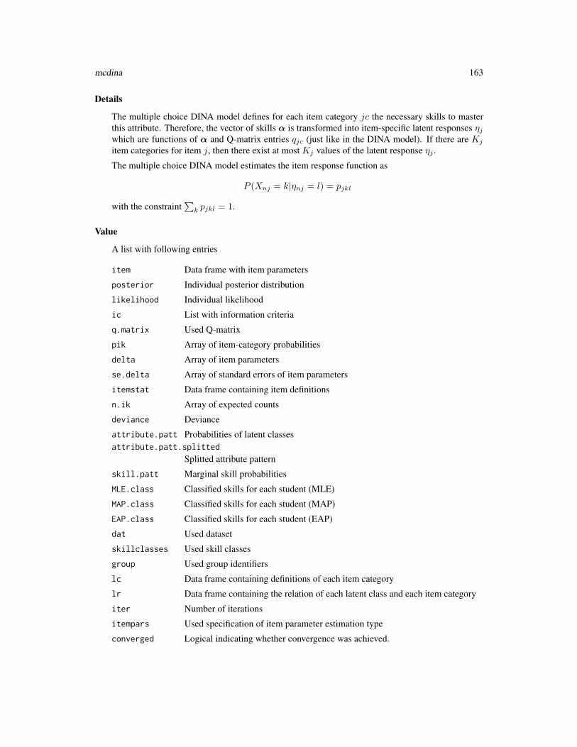
mcdina 163

Details

The multiple choice DINA model defines for each item category jc the necessary skills to masterthis attribute. Therefore, the vector of skills α is transformed into item-specific latent responses ηjwhich are functions of α and Q-matrix entries qjc (just like in the DINA model). If there are Kj

item categories for item j, then there exist at most Kj values of the latent response ηj .

The multiple choice DINA model estimates the item response function as

P (Xnj = k|ηnj = l) = pjkl

with the constraint∑k pjkl = 1.

Value


item Data frame with item parameters


likelihood Individual likelihood

ic List with information criteria


pik Array of item-category probabilities

delta Array of item parameters

se.delta Array of standard errors of item parameters

itemstat Data frame containing item definitions

n.ik Array of expected counts

deviance Deviance

attribute.patt Probabilities of latent classesattribute.patt.splitted

Splitted attribute pattern

skill.patt Marginal skill probabilities

MLE.class Classified skills for each student (MLE)

MAP.class Classified skills for each student (MAP)

EAP.class Classified skills for each student (EAP)

dat Used dataset

skillclasses Used skill classes

group Used group identifiers

lc Data frame containing definitions of each item category

lr Data frame containing the relation of each latent class and each item category


itempars Used specification of item parameter estimation type


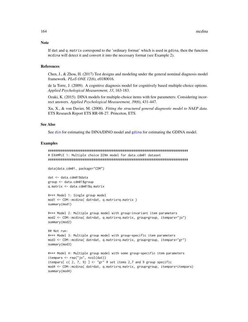
164 mcdina

Note

If dat and q.matrix correspond to the ’ordinary format’ which is used in gdina, then the functionmcdina will detect it and convert it into the necessary format (see Example 2).

References

Chen, J., & Zhou, H. (2017) Test designs and modeling under the general nominal diagnosis modelframework. PLoS ONE 12(6), e0180016.

de la Torre, J. (2009). A cognitive diagnosis model for cognitively based multiple-choice options.Applied Psychological Measurement, 33, 163-183.

Ozaki, K. (2015). DINA models for multiple-choice items with few parameters: Considering incor-rect answers. Applied Psychological Measurement, 39(6), 431-447.


See Also

See din for estimating the DINA/DINO model and gdina for estimating the GDINA model.

Examples

############################################################################## EXAMPLE 1: Multiple choice DINA model for data.cdm01 dataset#############################################################################


dat <- data.cdm01$datagroup <- data.cdm01$groupq.matrix <- data.cdm01$q.matrix

#*** Model 1: Single group modelmod1 <- CDM::mcdina( dat=dat, q.matrix=q.matrix )summary(mod1)

#*** Model 2: Multiple group model with group-invariant item parametersmod2 <- CDM::mcdina( dat=dat, q.matrix=q.matrix, group=group, itempars="jo")summary(mod2)

## Not run:#*** Model 3: Multiple group model with group-specific item parametersmod3 <- CDM::mcdina( dat=dat, q.matrix=q.matrix, group=group, itempars="gr")summary(mod3)

#*** Model 4: Multiple group model with some group-specific item parametersitempars <- rep("jo", ncol(dat))itempars[ c( 2, 7, 9) ] <- "gr" # set items 2,7 and 9 group specificmod4 <- CDM::mcdina( dat=dat, q.matrix=q.matrix, group=group, itempars=itempars)summary(mod4)

modelfit.cor 165

#*** Model 5: Reduced skill space

# define skill classesskillclasses <- scan(nlines=1) # read only one line

0 0 0 1 0 0 0 1 0 0 0 1 1 1 0 1 1 1skillclasses <- matrix( skillclasses, ncol=3, byrow=TRUE )mod5 <- CDM::mcdina( dat, q.matrix=q.matrix, group=group0, skillclasses=skillclasses )summary(mod5)

#*** Model 6: Reduced skill space with setting zero probabilities# for some latent classes

# set probabilities of classes P101 P011 (6th and 7th class) to zerozeroprob.skillclasses <- c(6,7)mod6 <- CDM::mcdina( dat, q.matrix, group=group, zeroprob.skillclasses=zeroprob.skillclasses )summary(mod6)

############################################################################## EXAMPLE 2: Using the mcdina function for estimating the DINA model#############################################################################


# estimate the DINA modelmod <- CDM::mcdina( sim.dina, q.matrix=sim.qmatrix )summary(mod)

############################################################################## EXAMPLE 3: MCDINA model with polytomous attributes#############################################################################

data(data.cdm02, package="CDM")dat <- data.cdm02$dataq.matrix <- data.cdm02$q.matrix

# estimate model with polytomous attribute B1mod1 <- CDM::mcdina( dat, q.matrix=q.matrix )summary(mod1)

## End(Not run)

modelfit.cor Assessing Model Fit and Local Dependence by Comparing Observedand Expected Item Pair Correlations

Description

This function computes several measures of absolute model fit and local dependence indices fordichotomous item responses which are based on comparing observed and expected frequencies ofitem pairs (Chen, de la Torre & Zhang, 2013; see Details).

166 modelfit.cor

Usage

modelfit.cor(data, posterior, probs)modelfit.cor2(data, posterior, probs)

modelfit.cor.din( dinobj, jkunits=0 )

## S3 method for class 'modelfit.cor.din'summary(object, ...)

Arguments

data An N × I data frame of dichotomous item responses

posterior A matrix containing the posterior distribution (e.g. obtained as an output of thedin function).

probs An array of dimension [items,categories,attribute classes] containing probabili-ties

dinobj An object of class din, gdina or gdm (only for dichotomous item responses)

object An object of class din, gdina or gdm (only for dichotomous item responses)

jkunits Number of Jackknife units. The default is to use 0 units (no use of jackknifing).If jackknife estimation should be employed, use (say) at least 20 jackknife units.The input jkunits can be also a vector of jackknife unit identifiers.


Details

The fit statistics are based on predictions of the pairwise table (Xi, Xj) of item responses. The χ2

statistic X2 for item pairs i and j is defined as

χ2ij =

1∑k=0

1∑l=0

(nij,kl − eij,kl)2

eij,kl

where nij,kl is the absolute frequency of {Xi = k,Xj = l} and eij,kl is the expected frequencyusing the estimated model. Note that for calculating eij,kl, individual posterior distributions areevaluated. The χ2

ij statistic is chi-square distributed with one degree of freedom and can be used fortesting whether items i and j are locally dependent. To control for multiple comparisons, p-valueadjustments according to the Holm and FDR method are conducted (see stats::p.adjust).

The residual covariance RESIDCOV of item pairs (i, j) is calculated as

RESIDCOVij =nij,11nij,00 − nij,10nij,01

n2− eij,11eij,00 − eij,10eij,01

n2

where MRESIDCOV is the average of all RESIDCOV statistics and is the total sample size.

The statistic MADcor denotes the average absolute deviation between observed correlations rij andmodel predicted correlations r̂ij of item pairs (i, j):

MADcor =1

J(J − 1)/2

∑i<j

|rij − r̂ij |

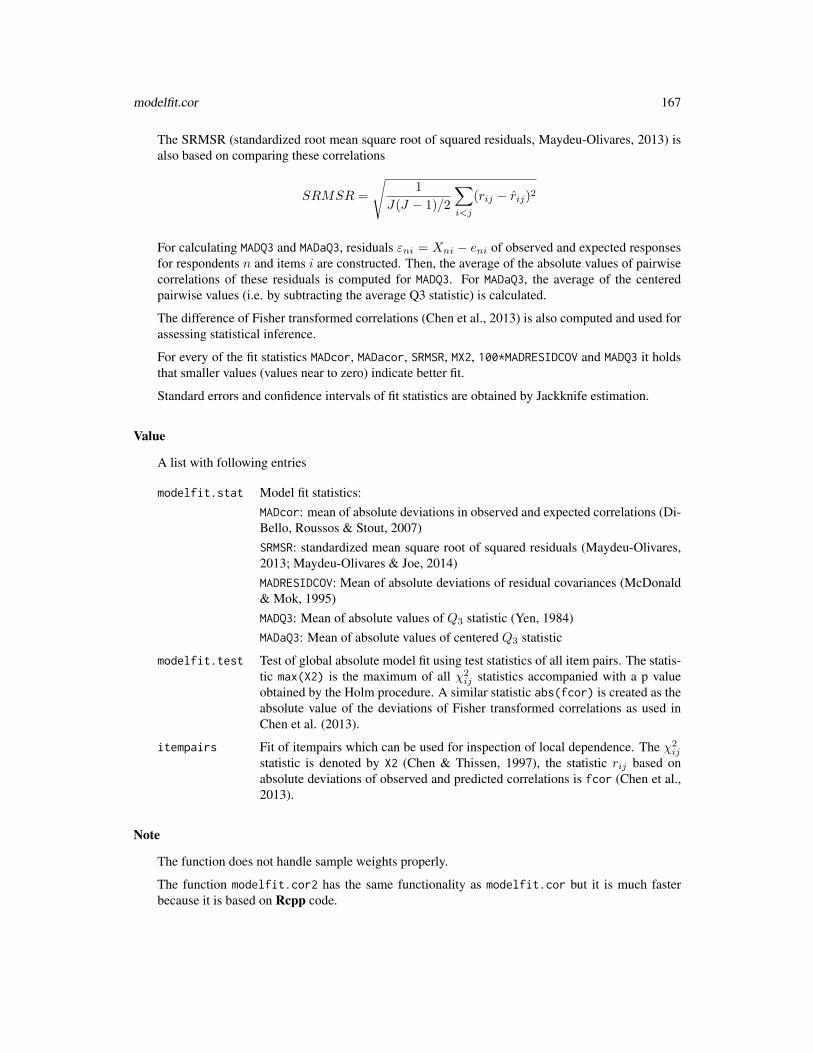
modelfit.cor 167

The SRMSR (standardized root mean square root of squared residuals, Maydeu-Olivares, 2013) isalso based on comparing these correlations

SRMSR =

√1

J(J − 1)/2

∑i<j

(rij − r̂ij)2

For calculating MADQ3 and MADaQ3, residuals εni = Xni − eni of observed and expected responsesfor respondents n and items i are constructed. Then, the average of the absolute values of pairwisecorrelations of these residuals is computed for MADQ3. For MADaQ3, the average of the centeredpairwise values (i.e. by subtracting the average Q3 statistic) is calculated.

The difference of Fisher transformed correlations (Chen et al., 2013) is also computed and used forassessing statistical inference.

For every of the fit statistics MADcor, MADacor, SRMSR, MX2, 100*MADRESIDCOV and MADQ3 it holdsthat smaller values (values near to zero) indicate better fit.

Standard errors and confidence intervals of fit statistics are obtained by Jackknife estimation.

Value


modelfit.stat Model fit statistics:MADcor: mean of absolute deviations in observed and expected correlations (Di-Bello, Roussos & Stout, 2007)SRMSR: standardized mean square root of squared residuals (Maydeu-Olivares,2013; Maydeu-Olivares & Joe, 2014)MADRESIDCOV: Mean of absolute deviations of residual covariances (McDonald& Mok, 1995)MADQ3: Mean of absolute values of Q3 statistic (Yen, 1984)MADaQ3: Mean of absolute values of centered Q3 statistic

modelfit.test Test of global absolute model fit using test statistics of all item pairs. The statis-tic max(X2) is the maximum of all χ2

ij statistics accompanied with a p valueobtained by the Holm procedure. A similar statistic abs(fcor) is created as theabsolute value of the deviations of Fisher transformed correlations as used inChen et al. (2013).

itempairs Fit of itempairs which can be used for inspection of local dependence. The χ2ij

statistic is denoted by X2 (Chen & Thissen, 1997), the statistic rij based onabsolute deviations of observed and predicted correlations is fcor (Chen et al.,2013).

Note

The function does not handle sample weights properly.

The function modelfit.cor2 has the same functionality as modelfit.cor but it is much fasterbecause it is based on Rcpp code.

168 modelfit.cor

References

Chen, J., de la Torre, J., & Zhang, Z. (2013). Relative and absolute fit evaluation in cognitivediagnosis modeling. Journal of Educational Measurement, 50, 123-140.

Chen, W., & Thissen, D. (1997). Local dependence indexes for item pairs using item responsetheory. Journal of Educational and Behavioral Statistics, 22, 265-289.

DiBello, L. V., Roussos, L. A., & Stout, W. F. (2007). Review of cognitively diagnostic assess-ment and a summary of psychometric models. In C. R. Rao and S. Sinharay (Eds.), Handbook ofStatistics, Vol. 26 (pp. 979–1030). Amsterdam: Elsevier.

Maydeu-Olivares, A. (2013). Goodness-of-fit assessment of item response theory models (withdiscussion). Measurement: Interdisciplinary Research and Perspectives, 11, 71-137.

Maydeu-Olivares, A., & Joe, H. (2014). Assessing approximate fit in categorical data analysis.Multivariate Behavioral Research, 49, 305-328.

McDonald, R. P., & Mok, M. M.-C. (1995). Goodness of fit in item response models. MultivariateBehavioral Research, 30, 23-40.

Yen, W. M. (1984). Effects of local item dependence on the fit and equating performance of thethree-parameter logistic model. Applied Psychological Measurement, 8, 125-145.

Examples

## Not run:############################################################################## EXAMPLE 1: Model fit for sim.dina#############################################################################

data(sim.dina, package="CDM")data(sim.qmatrix, package="CDM")dat <- sim.dinaq.matrix <- sim.qmatrix

#*** Model 1: DINA model for DINA simulated datamod1 <- CDM::din(dat, q.matrix=q.matrix, rule="DINA" )fmod1 <- CDM::modelfit.cor.din(mod1, jkunits=10)summary(fmod1)

## Test of Global Model Fit## type value p## 1 max(X2) 8.728 0.113## 2 abs(fcor) 0.143 0.080#### Fit Statistics## est jkunits jk_est jk_se est_low est_upp## MADcor 0.030 10 0.020 0.005 0.010 0.030## SRMSR 0.040 10 0.023 0.006 0.011 0.035## 100*MADRESIDCOV 0.671 10 0.445 0.125 0.200 0.690## MADQ3 0.062 10 0.037 0.008 0.021 0.052## MADaQ3 0.059 10 0.034 0.008 0.019 0.050

# look at first five item pairs with highest degree of local dependenceitempairs <- fmod1$itempairsitempairs <- itempairs[ order( itempairs$X2, decreasing=TRUE ), ]

modelfit.cor 169

itempairs[ 1:5, c("item1","item2", "X2", "X2_p", "X2_p.holm", "Q3") ]## item1 item2 X2 X2_p X2_p.holm Q3## 29 Item5 Item8 8.728248 0.003133174 0.1127943 -0.26616414## 32 Item6 Item8 2.644912 0.103881881 1.0000000 0.04873154## 21 Item3 Item9 2.195011 0.138458201 1.0000000 0.05948456## 10 Item2 Item4 1.449106 0.228671389 1.0000000 -0.08036216## 30 Item5 Item9 1.393583 0.237800911 1.0000000 -0.01934420

#*** Model 2: DINO model for DINA simulated datamod2 <- CDM::din(dat, q.matrix=q.matrix, rule="DINO" )fmod2 <- CDM::modelfit.cor.din(mod2, jkunits=10 ) # 10 jackknife unitssummary(fmod2)


#*** Model 3: estimate DINA model with gdina functionmod3 <- CDM::gdina( dat, q.matrix=q.matrix, rule="DINA" )fmod3 <- CDM::modelfit.cor.din( mod3, jkunits=0 ) # no Jackknife estimationsummary(fmod3)

## Test of Global Model Fit## type value p## 1 max(X2) 8.756 0.111## 2 abs(fcor) 0.143 0.078#### Fit Statistics## est## MADcor 0.030## SRMSR 0.040## MX2 0.719## 100*MADRESIDCOV 0.668## MADQ3 0.062## MADaQ3 0.059

############################################################################## EXAMPLE 2: Simulated Example DINA model#############################################################################

set.seed(9765)# specify Q-matrixQ <- matrix( c(1,0, 0,1, 1,1 ), nrow=3, ncol=2, byrow=TRUE )q.matrix <- Q[ rep(1:3,4), ]I <- nrow(q.matrix)

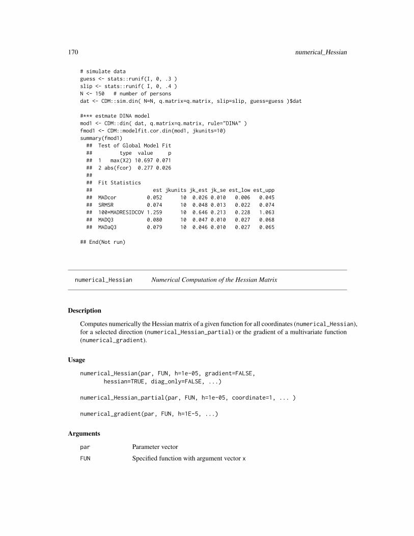
170 numerical_Hessian

# simulate dataguess <- stats::runif(I, 0, .3 )slip <- stats::runif( I, 0, .4 )N <- 150 # number of personsdat <- CDM::sim.din( N=N, q.matrix=q.matrix, slip=slip, guess=guess )$dat

#*** estmate DINA modelmod1 <- CDM::din( dat, q.matrix=q.matrix, rule="DINA" )fmod1 <- CDM::modelfit.cor.din(mod1, jkunits=10)summary(fmod1)


## End(Not run)

numerical_Hessian Numerical Computation of the Hessian Matrix

Description

Computes numerically the Hessian matrix of a given function for all coordinates (numerical_Hessian),for a selected direction (numerical_Hessian_partial) or the gradient of a multivariate function(numerical_gradient).

Usage

numerical_Hessian(par, FUN, h=1e-05, gradient=FALSE,hessian=TRUE, diag_only=FALSE, ...)

numerical_Hessian_partial(par, FUN, h=1e-05, coordinate=1, ... )

numerical_gradient(par, FUN, h=1E-5, ...)

Arguments

par Parameter vector

FUN Specified function with argument vector x

numerical_Hessian 171

h Numerical differentiation parameter. Can be also a vector. The increment in thenumerical approximation of the derivative is defined as hi max(1, θi) where θidenotes the ith parameter.

gradient Logical indicating whether the gradient should be calculated.

hessian Logical indicating whether the Hessian matrix should be calculated.

diag_only Logical indicating whether only the diagonal of the hessian should be computed.

... Further arguments to be passed to FUN.

coordinate Coordinate index for partial derivative

Value

Gradient vector or Hessian matrix or a list of both elements

See Also

See the numDeriv package and the mirt::numerical_deriv function from the mirt package.

Examples

############################################################################## EXAMPLE 1: Toy example for Hessian matrix#############################################################################

# define functionf <- function(x){

3*x[1]^3 - 4*x[2]^2 - 5*x[1]*x[2] + 10 * x[1] * x[3]^2 + 6*x[2]*sqrt(x[3])}# define point for evaluating partial derivativespar <- c(3,8,4)

#--- compute gradientCDM::numerical_Hessian( par=par, FUN=f, gradient=TRUE, hessian=FALSE)## Not run:mirt::numerical_deriv(par=par, f=f, gradient=TRUE)

#--- compute Hessian matrixCDM::numerical_Hessian( par=par, FUN=f )mirt::numerical_deriv(par=par, f=f, gradient=FALSE)numerical_Hessian( par=par, FUN=f, h=1E-4 )

#--- compute gradient and Hessian matrixCDM::numerical_Hessian( par=par, FUN=f, gradient=TRUE, hessian=TRUE)

## End(Not run)

172 osink

osink Opens and Closes a sink Connection

Description

Opens and closes a sink connection.

Usage

osink(file, suffix, append=FALSE)

csink(file)

Arguments

file File name. No sink is done if it has the value NULL.

suffix Suffix which should be put next to the file name

append Optional logical indicating whether console output should be appended to analready existing file. See argument append in base::sink.

See Also

base::sink

Examples

## The function 'osink' is currently defined asfunction (file, suffix){

if (!is.null(file)) {base::sink(paste0(file, suffix), split=TRUE)}

}

## The function 'csink' is currently defined asfunction (file){

if (!is.null(file)) {base::sink()}

}

personfit.appropriateness 173

personfit.appropriateness

Appropriateness Statistic for Person Fit Assessment

Description

This function computes the person fit appropriateness statistics (Levine & Drasgow, 1988) as pro-posed for cognitive diagnostic models by Liu, Douglas and Henson (2009). The appropriatenessstatistic assesses spuriously high scorers (attr.type=1) and spuriously low scorers (attr.type=0).

Usage

personfit.appropriateness(data, probs, skillclassprobs, h=0.001, eps=1e-10,maxiter=30, conv=1e-05, max.increment=0.1, progress=TRUE)

## S3 method for class 'personfit.appropriateness'summary(object, digits=3, ...)

## S3 method for class 'personfit.appropriateness'plot(x, cexpch=.65, ...)

Arguments

data Data frame of dichotomous item responses

probs Probabilities evaluated at skill space (abilities θ)

skillclassprobs

Probabilities of skill classes

h Numerical differentiation parameter

eps Constant which is added to probabilities avoiding zero probability


conv Convergence criterion

max.increment Maximum increment in iteration

progress Optional logical indicating whether iteration progress should be displayed.

object Object of class personfit.appropriateness

digits Number of digits for rounding

x Object of class personfit.appropriateness

cexpch Point size in plot


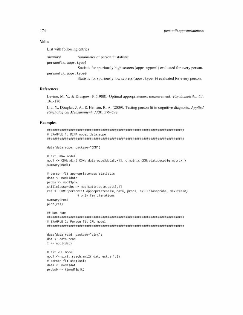
174 personfit.appropriateness

Value


summary Summaries of person fit statisticpersonfit.appr.type1

Statistic for spuriously high scorers (appr.type=1) evaluated for every person.personfit.appr.type0

Statistic for spuriously low scorers (appr.type=0) evaluated for every person.

References

Levine, M. V., & Drasgow, F. (1988). Optimal appropriateness measurement. Psychometrika, 53,161-176.

Liu, Y., Douglas, J. A., & Henson, R. A. (2009). Testing person fit in cognitive diagnosis. AppliedPsychological Measurement, 33(8), 579-598.

Examples

############################################################################## EXAMPLE 1: DINA model data.ecpe#############################################################################

data(data.ecpe, package="CDM")

# fit DINA modelmod1 <- CDM::din( CDM::data.ecpe$data[,-1], q.matrix=CDM::data.ecpe$q.matrix )summary(mod1)

# person fit appropriateness statisticdata <- mod1$dataprobs <- mod1$pjkskillclassprobs <- mod1$attribute.patt[,1]res <- CDM::personfit.appropriateness( data, probs, skillclassprobs, maxiter=8)

# only few iterationssummary(res)plot(res)

## Not run:############################################################################## EXAMPLE 2: Person fit 2PL model#############################################################################

data(data.read, package="sirt")dat <- data.readI <- ncol(dat)

# fit 2PL modelmod1 <- sirt::rasch.mml2( dat, est.a=1:I)# person fit statisticdata <- mod1$datprobs0 <- t(mod1$pjk)

plot.din 175

probs <- array( 0, dim=c( I, 2, dim(probs0)[2] ) )probs[,2,] <- probs0probs[,1,] <- 1 - probs0skillclassprobs <- mod1$trait.distr$pi.kres <- CDM::personfit.appropriateness( data, probs, skillclassprobs )summary(res)plot(res)

## End(Not run)

plot.din Plot Method for Objects of Class din

Description

S3 method to plot objects of the class din.

Usage

## S3 method for class 'din'plot(x, items=c(1:ncol(x$data)), pattern="",

uncertainty=0.1, top.n.skill.classes=6, pdf.file="",hide.obs=FALSE, display.nr=1:4, ask=TRUE, ...)

Arguments

x A required object of class din, obtained from a call to the function din.

items An index vector giving the items to be visualized in the first plot, see ‘Details’.The default is items=c(1:ncol(x$data)), which is all items.

pattern An optional character or a numeric vector specifying a response pattern of anrespondent, whose attributes are analyzed in a separate graphic. It is required tochoose a pattern from the empirical data set (see Example).

uncertainty A numeric between 0 and 0.5 giving the uncertainty bounds for deriving theobserved skill occurrence probabilities in plot 2 and the simplified deterministicattribute profiles in plot 4.

top.n.skill.classes

A numeric, specifying the number of skill classes, starting with the most fre-quent, to be labeled in plot 3. Default value is 6.

pdf.file An optional character string. If specified the graphics obtained from the functionplot.din are provided in a pdf file. The default is pdf.file="", which is notproviding a pdf file. Otherwise specify a directory and filename ending with.pdf where to write the document.

hide.obs An optional logical value. If set to TRUE, the polygonal chain for observed fre-quencies of skill class probabilities in the second graphic is not displayed.

display.nr An optional numeric or numeric vector. If specified, only the plots in display.nrare displayed. Default is display.nr=1:4 causing the display of all four plots.

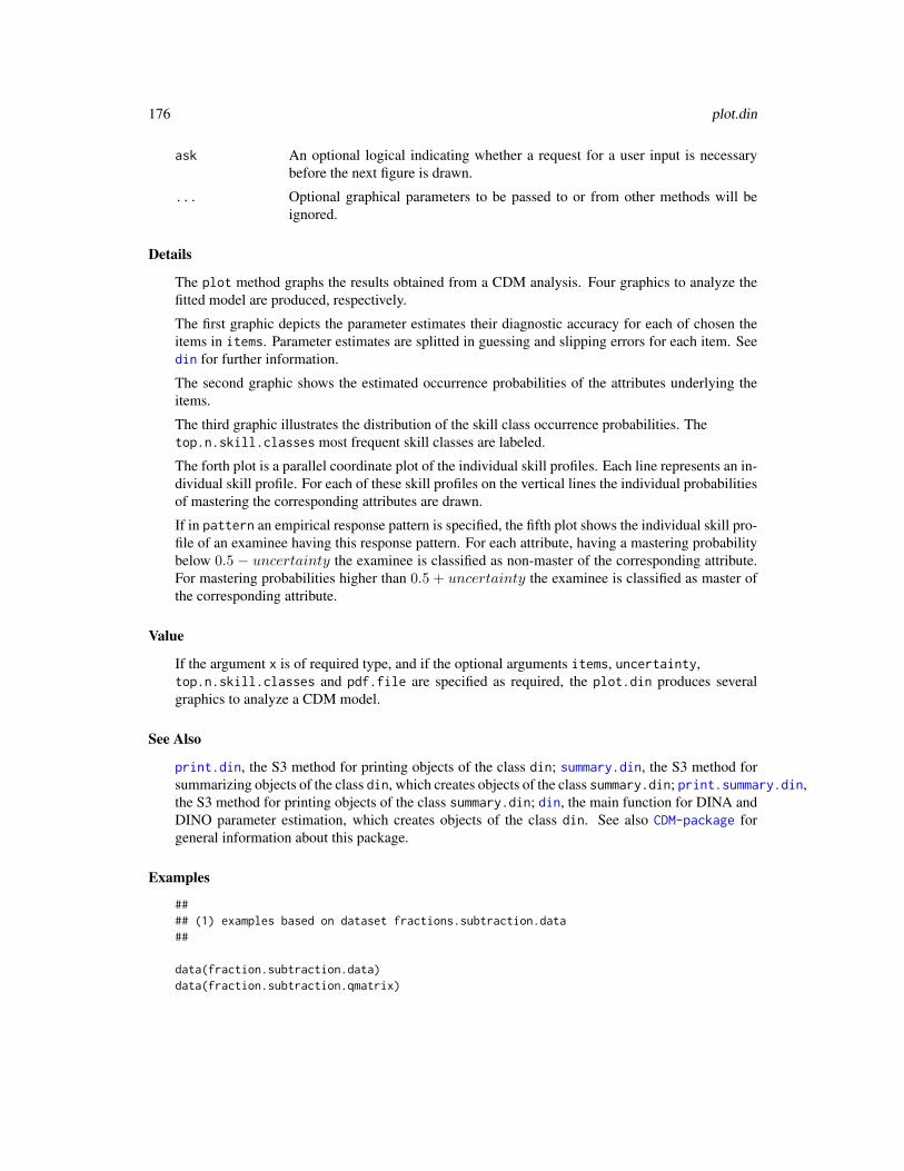
176 plot.din

ask An optional logical indicating whether a request for a user input is necessarybefore the next figure is drawn.

... Optional graphical parameters to be passed to or from other methods will beignored.

Details

The plot method graphs the results obtained from a CDM analysis. Four graphics to analyze thefitted model are produced, respectively.

The first graphic depicts the parameter estimates their diagnostic accuracy for each of chosen theitems in items. Parameter estimates are splitted in guessing and slipping errors for each item. Seedin for further information.

The second graphic shows the estimated occurrence probabilities of the attributes underlying theitems.

The third graphic illustrates the distribution of the skill class occurrence probabilities. Thetop.n.skill.classes most frequent skill classes are labeled.

The forth plot is a parallel coordinate plot of the individual skill profiles. Each line represents an in-dividual skill profile. For each of these skill profiles on the vertical lines the individual probabilitiesof mastering the corresponding attributes are drawn.

If in pattern an empirical response pattern is specified, the fifth plot shows the individual skill pro-file of an examinee having this response pattern. For each attribute, having a mastering probabilitybelow 0.5 − uncertainty the examinee is classified as non-master of the corresponding attribute.For mastering probabilities higher than 0.5 + uncertainty the examinee is classified as master ofthe corresponding attribute.

Value

If the argument x is of required type, and if the optional arguments items, uncertainty,top.n.skill.classes and pdf.file are specified as required, the plot.din produces severalgraphics to analyze a CDM model.

See Also

print.din, the S3 method for printing objects of the class din; summary.din, the S3 method forsummarizing objects of the class din, which creates objects of the class summary.din; print.summary.din,the S3 method for printing objects of the class summary.din; din, the main function for DINA andDINO parameter estimation, which creates objects of the class din. See also CDM-package forgeneral information about this package.

Examples

#### (1) examples based on dataset fractions.subtraction.data##

data(fraction.subtraction.data)data(fraction.subtraction.qmatrix)

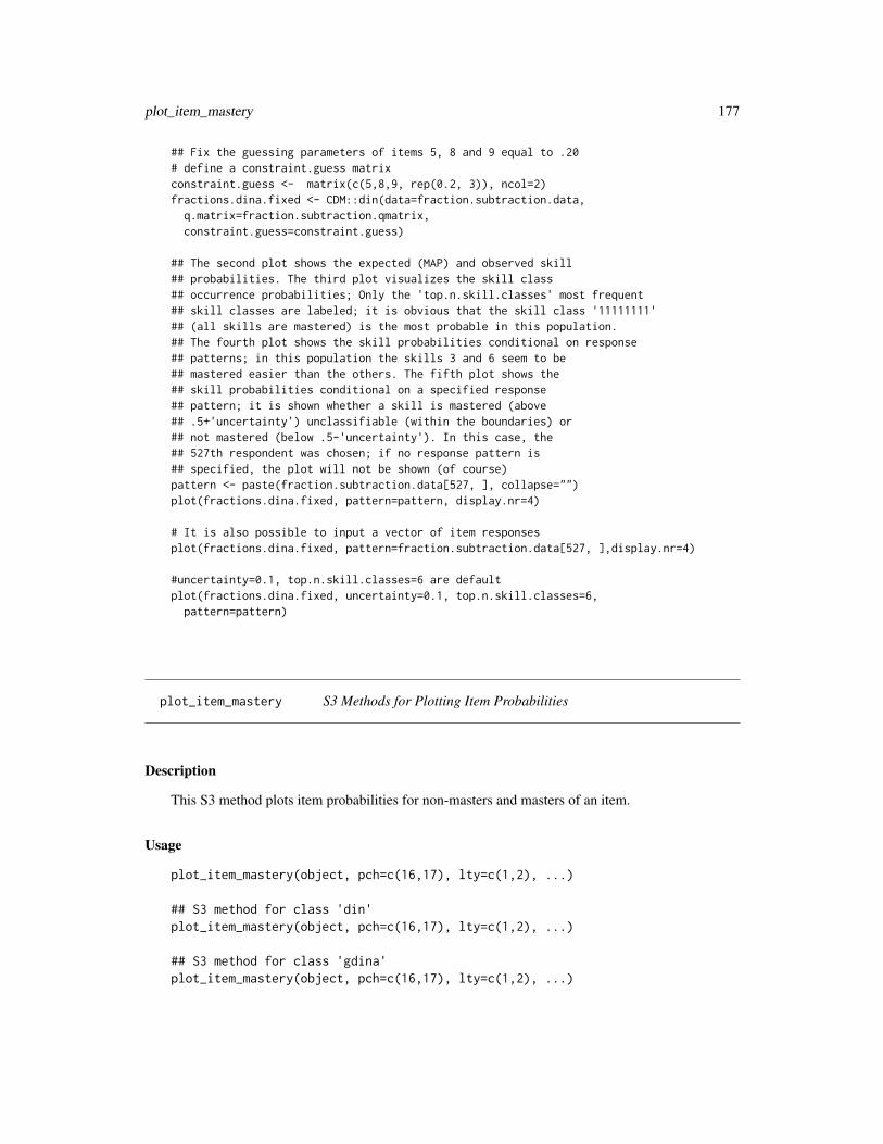
plot_item_mastery 177

## Fix the guessing parameters of items 5, 8 and 9 equal to .20# define a constraint.guess matrixconstraint.guess <- matrix(c(5,8,9, rep(0.2, 3)), ncol=2)fractions.dina.fixed <- CDM::din(data=fraction.subtraction.data,

q.matrix=fraction.subtraction.qmatrix,constraint.guess=constraint.guess)

## The second plot shows the expected (MAP) and observed skill## probabilities. The third plot visualizes the skill class## occurrence probabilities; Only the 'top.n.skill.classes' most frequent## skill classes are labeled; it is obvious that the skill class '11111111'## (all skills are mastered) is the most probable in this population.## The fourth plot shows the skill probabilities conditional on response## patterns; in this population the skills 3 and 6 seem to be## mastered easier than the others. The fifth plot shows the## skill probabilities conditional on a specified response## pattern; it is shown whether a skill is mastered (above## .5+'uncertainty') unclassifiable (within the boundaries) or## not mastered (below .5-'uncertainty'). In this case, the## 527th respondent was chosen; if no response pattern is## specified, the plot will not be shown (of course)pattern <- paste(fraction.subtraction.data[527, ], collapse="")plot(fractions.dina.fixed, pattern=pattern, display.nr=4)

# It is also possible to input a vector of item responsesplot(fractions.dina.fixed, pattern=fraction.subtraction.data[527, ],display.nr=4)

#uncertainty=0.1, top.n.skill.classes=6 are defaultplot(fractions.dina.fixed, uncertainty=0.1, top.n.skill.classes=6,

pattern=pattern)

plot_item_mastery S3 Methods for Plotting Item Probabilities

Description

This S3 method plots item probabilities for non-masters and masters of an item.

Usage

plot_item_mastery(object, pch=c(16,17), lty=c(1,2), ...)

## S3 method for class 'din'plot_item_mastery(object, pch=c(16,17), lty=c(1,2), ...)

## S3 method for class 'gdina'plot_item_mastery(object, pch=c(16,17), lty=c(1,2), ...)

178 predict

Arguments

object Object of classes din or gdina

pch Point symbols for both groups

lty Line symbols for both groups


Value

Plot

See Also

Plot functions for item response curves: IRT.irfprobPlot.

Examples

## Not run:############################################################################## EXAMPLE 1: Plot item mastery#############################################################################

data(sim.dina)data(sim.qmatrix)

#* estimate DINA Modelmod1 <- CDM::din(sim.dina, q.matrix=sim.qmatrix, rule="DINA")#* estimate GDINA modelmod2 <- CDM::gdina(sim.dina, q.matrix=sim.qmatrix)

#* plotsplot_item_mastery(mod1)plot_item_mastery(mod2)

## End(Not run)

predict Expected Values and Predicted Probabilities from Item Response Re-sponse Models

Description

This function computes expected values for each person and each item based on the individualposterior distribution. The output of this function can be the basis of creating item and person fitstatistics.

predict 179

Usage

IRT.predict(object, dat, group=1)

## S3 method for class 'din'predict(object, group=1, ...)

## S3 method for class 'gdina'predict(object, group=1, ...)

## S3 method for class 'mcdina'predict(object, group=1, ...)

## S3 method for class 'gdm'predict(object, group=1, ...)

## S3 method for class 'slca'predict(object, group=1, ...)

Arguments

object Object for the S3 methods IRT.irfprob and IRT.posterior are defined. Inthe CDM packages, these are the objects of class din, gdina, mcdina, slca orgdm.

dat Dataset with item responses

group Group index for use


Value


expected Array with expected values (persons × classes × items)

probs.categ Array with expected probabilities for each category (persons × categories ×classes × items)

variance Array with variance in predicted values for each person and each item.

residuals Array with residuals for each person and each item

stand.resid Array with standardized residuals for each person and each item

Examples

## Not run:############################################################################## EXAMPLE 1: Fitted Rasch model in TAM package#############################################################################

#--- Model 1: Rasch modellibrary(TAM)

180 print.summary.din

mod1 <- TAM::tam.mml(resp=TAM::sim.rasch)# apply IRT.predict functionprmod1 <- CDM::IRT.predict(mod1, mod1$resp )str(prmod1)

## End(Not run)

############################################################################## EXAMPLE 2: Predict function for din#############################################################################

# DINA Modelmod1 <- CDM::din( CDM::sim.dina, q.matr=CDM::sim.qmatrix, rule="DINA" )summary(mod1)# apply predict methodprmod1 <- CDM::IRT.predict( mod1, sim.dina )str(prmod1)

print.summary.din Print Method for Objects of Class summary.din

Description

S3 method to print objects of the class summary.din.

Usage

## S3 method for class 'summary.din'print(x, ...)

Arguments

x A required object of class summary.din, obtained from a call to the functionsummary.din (through generic function summary).


Details

The print method prints the summary information about objects of the class din computed bysummary.din, which are the item discriminations indices, the most frequent skill classes and themodel information criteria AIC and BIC. Specific summary information details such as individualitems with their discrimination index can be accessed through assignment (see ‘Examples’).

Value

If the argument x is of required type, print.summary.din prints the summary information in ‘De-tails’, and invisibly returns x.

reglca 181

See Also

plot.din, the S3 method for plotting objects of the class din; print.din, the S3 method forprinting objects of the class din; summary.din, the S3 method for summarizing objects of the classdin, which creates objects of the class summary.din; din, the main function for DINA and DINOparameter estimation, which creates objects of the class din. See also CDM-package for generalinformation about this package.

Examples


## In particular, accessing detailed summary through assignmentmod <- CDM::din(data=CDM::fraction.subtraction.data,

q.matrix=CDM::fraction.subtraction.qmatrix, rule="DINA")smod <- summary(mod)str(smod)

reglca Regularized Latent Class Analysis

Description

Estimates the regularized latent class model for dichotomous responses based on regularizationmethods (Chen, Liu, Xu, & Ying, 2015; Chen, Li, Liu, & Ying, 2017). The SCAD and MCPpenalty functions are available.

Usage

reglca(dat, nclasses, weights=NULL, group=NULL, regular_type="scad",regular_lam=0, sd_noise_init=1, item_probs_init=NULL, class_probs_init=NULL,random_starts=1, random_iter=20, conv=1e-05, h=1e-04, mstep_iter=10,maxit=1000, verbose=TRUE, prob_min=.0001)

## S3 method for class 'reglca'summary(object, digits=4, file=NULL, ...)

Arguments

dat Matrix with dichotomous item responses. NAs are allowed.

nclasses Number of classes

weights Optional vector of sampling weights

group Optional vector for grouping variable

regular_type Regularization type. Can be scad or mcp. See gdina for more information.


182 reglca

sd_noise_init Standard deviation for amount of noise in generating random starting valuesitem_probs_init

Optional matrix of initial item response probabilitiesclass_probs_init

Optional vector of class probabilitiesrandom_starts Number of random startsrandom_iter Number of initial iterations for random startsconv Convergence criterionh Numerical differentiation parametermstep_iter Number of iterations in the M-stepmaxit Maximum number of iterationsverbose Logical indicating whether convergence progress should be displayedprob_min Lower bound for probabilities in estimationobject A required object of class gdina, obtained from a call to the function gdina.digits Number of digits after decimal separator to display.file Optional file name for a file in which summary should be sinked.... Further arguments to be passed.

Details

The regularized latent class model for dichotomous item responses assumes C latent classes. Theitem response probabilities P (Xi = 1|c) = pic are estimated in such a way such that the numberof different pic values per item is minimized. This approach eases interpretability and enables torecover the structure of a true (but unknown) cognitive diagnostic model.

Value

A list containing following elements (selection):

item_probs Item response probabilitiesclass_probs Latent class probabilitiesp.aj.xi Individual posteriorp.xi.aj Individual likelihoodloglike Log-likelihood valueNpars Number of estimated parametersNskillpar Number of skill class parametersG Number of groupsn.ik Expected countsNipar Number of item parametersn_reg Number of regularized parametersn_reg_item Number of regularized parameters per itemitem Data frame with item parameterspjk Item response probabilities (in an array)N Number of personsI Number of items

reglca 183

References

Chen, Y., Liu, J., Xu, G., & Ying, Z. (2015). Statistical analysis of Q-matrix based diagnosticclassification models. Journal of the American Statistical Association, 110, 850-866.


See Also

See also the gdina and slca functions for regularized estimation.

Examples

## Not run:############################################################################## EXAMPLE 1: Estimating a regularized LCA for DINA data#############################################################################

#---- simulate dataI <- 12 # number of items# define Q-matrixq.matrix <- matrix(0,I,2)q.matrix[ 1:(I/3), 1 ] <- 1q.matrix[ I/3 + 1:(I/3), 2 ] <- 1q.matrix[ 2*I/3 + 1:(I/3), c(1,2) ] <- 1N <- 1000 # number of personsguess <- rep(seq(.1,.3,length=I/3), 3)slip <- .1rho <- 0.3 # skill correlationset.seed(987)dat <- CDM::sim.din( N=N, q.matrix=q.matrix, guess=guess, slip=slip,

mean=0*c( .2, -.2 ), Sigma=matrix( c( 1, rho,rho,1), 2, 2 ) )dat <- dat$dat

#--- Model 1: Four latent classes without regularizationmod1 <- CDM::reglca(dat=dat, nclasses=4, regular_lam=0, random_starts=3,

random_iter=10, conv=1E-4)summary(mod1)

#--- Model 2: Four latent classes with regularization and lambda=.08mod2 <- CDM::reglca(dat=dat, nclasses=4, regular_lam=0.08, regular_type="scad",

random_starts=3, random_iter=10, conv=1E-4)summary(mod2)

#--- Model 3: Four latent classes with regularization and lambda=.05 with warm start

# "warm start" -> use initial parameters from fitted model with higher lambda valueitem_probs_init <- mod2$item_probsclass_probs_init <- mod2$class_probsmod3 <- CDM::reglca(dat=dat, nclasses=4, regular_lam=0.05, regular_type="scad",

item_probs_init=item_probs_init, class_probs_init=class_probs_init,random_starts=3, random_iter=10, conv=1E-4)

184 sequential.items

## End(Not run)

sequential.items Constructing a Dataset with Sequential Pseudo Items for Ordered ItemResponses

Description

This function constructs dichotomous pseudo items from polytomous ordered items (Tutz, 1997).Using this method, developed test models for dichotomous data can be applied for polytomous itemresponses after transforming them into dichotomous data. See Details for the construction.

Ma and de la Torre (2016) proposed a sequential GDINA model. Interestingly, the proposed modelcan be fitted with the gdina function in this CDM package while item responses has to be trans-formed with the sequential.items function for obtaining dichotomous pseudoitems. The Q-matrix for the sequential model of Ma and de la Torre (2016) can be used in the GDINA model forthe dichotomous pseudoitems. This approach is implemented for automatic use in gdina.

Usage

sequential.items(data)

Arguments

data A data frame with item responses

Details

Assume that item j possesses K ≥ 3 categories. We label these categories as k = 0, 1, . . . ,K − 1.The original item responsesXnj for person n at item j is then transformed intoK−1 pseudo itemsYj1, . . . , Yj,K−1.

The first pseudo item response Ynj1 is defined as 1 iff Xnj ≥ 1. The second item responses Ynj2is 1 iff Xnj ≥ 2, it is 0 iff Xnj = 1 and it is missing (NA in the dataset) iff Xnj = 0. Theconstruction proceeds in the same manner for other categories (see Tutz, 1997). The pseudo itemscan be recognized as ’hurdles’ a participant has to master to get a score of k for the original item.

The pseudo items are treated as conditionally independent which implies that IRT models or CDMswhich assume local independence can be employed for estimation.

For deriving item response probabilities of the original items from response probabilities of thepseudo items see Tutz (1997, p. 141ff.).

Value


dat.expand A data frame with dichotomous pseudo items

iteminfo A data frame containing some item information

maxK Vector with maximum number of categories per item

sequential.items 185

References

Ma, W., & de la Torre, J. (2016). A sequential cognitive diagnosis model for polytomous responses.British Journal of Mathematical and Statistical Psychology, 69(3), 253-275.

Tutz, G. (1997). Sequential models for ordered responses. In W. van der Linden & R. K. Hambleton.Handbook of modern item response theory (pp. 139-152). New York: Springer.

Examples

############################################################################## EXAMPLE 1: Constructing sequential pseudo items for data.mg#############################################################################

data(data.mg, package="CDM")dat <- data.mgitems <- colnames(dat)[ which( substring( colnames(dat),1,1)=="I" ) ]## [1] "I1" "I2" "I3" "I4" "I5" "I6" "I7" "I8" "I9" "I10" "I11"data <- dat[,items]

# construct sequential dichotomous pseudo itemsres <- CDM::sequential.items(data)

# item information tableres$iteminfo

## item itemindex category pseudoitem## 1 I1 1 1 I1## 2 I2 2 1 I2## 3 I3 3 1 I3## 4 I4 4 1 I4_Cat1## 5 I4 4 2 I4_Cat2## 6 I5 5 1 I5_Cat1## 7 I5 5 2 I5_Cat2## [...]

# extract dataset with pseudo itemsdat.expand <- res$dat.expandcolnames(dat.expand)

## [1] "I1" "I2" "I3" "I4_Cat1" "I4_Cat2" "I5_Cat1"## [7] "I5_Cat2" "I6_Cat1" "I6_Cat2" "I7_Cat1" "I7_Cat2" "I7_Cat3"## [13] "I8" "I9" "I10" "I11_Cat1" "I11_Cat2" "I11_Cat3"

# compare original items and pseudoitems

#**** Item I1stats::xtabs( ~ paste(data$I1) + paste(dat.expand$I1) )

## paste(dat.expand$I1)## paste(data$I1) 0 1 NA## 0 4339 0 0## 1 0 33326 0## NA 0 0 578

#**** Item I7

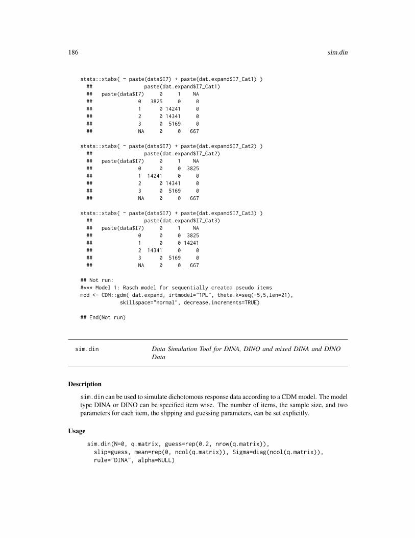
186 sim.din

stats::xtabs( ~ paste(data$I7) + paste(dat.expand$I7_Cat1) )## paste(dat.expand$I7_Cat1)## paste(data$I7) 0 1 NA## 0 3825 0 0## 1 0 14241 0## 2 0 14341 0## 3 0 5169 0## NA 0 0 667



## Not run:#*** Model 1: Rasch model for sequentially created pseudo itemsmod <- CDM::gdm( dat.expand, irtmodel="1PL", theta.k=seq(-5,5,len=21),

skillspace="normal", decrease.increments=TRUE)

## End(Not run)

sim.din Data Simulation Tool for DINA, DINO and mixed DINA and DINOData

Description

sim.din can be used to simulate dichotomous response data according to a CDM model. The modeltype DINA or DINO can be specified item wise. The number of items, the sample size, and twoparameters for each item, the slipping and guessing parameters, can be set explicitly.

Usage

sim.din(N=0, q.matrix, guess=rep(0.2, nrow(q.matrix)),slip=guess, mean=rep(0, ncol(q.matrix)), Sigma=diag(ncol(q.matrix)),rule="DINA", alpha=NULL)

sim.din 187

Arguments

N A numeric value specifying the number N of requested response patterns. Ifalpha is specified, then N is set by default to 0.

q.matrix A required binary J × K matrix describing which of the K attributes are re-quired, coded by 1, and which attributes are not required, coded by 0, to masterthe items.

guess An optional vector of guessing parameters. Default is 0.2 for each item.

slip An optional vector of slipping parameters. Default is 0.2 for each item.

mean A numeric vector of length ncol(q.matrix) indicating the mean vector of thecontinuous version of the dichotomous skill vector. Default is rep(0,length=ncol(q.matrix)).That is, having a probability of 0.5 for possessing each of the attributes.

Sigma A matrix of dimension ncol(q.matrix) times ncol(q.matrix) specifying thecovariance matrix of the continuous version of the dichotomous skill vector (i.e.,the tetrachoric correlation of the dichotomous skill vector). Default is diag(1,ncol(q.matrix)). That is, by default the possession of the attributes is as-sumed to be uncorrelated.

rule An optional character string or vector of character strings specifying the modelrule that is used. The character strings must be of "DINA" or "DINO". If a vectorof character strings is specified, implying an itemwise condensation rule, thevector must be of length J , which is the number of used items. The default isthe condensation rule "DINA" for all items.

alpha A matrix of attribute patterns which can be given as an input instead of underly-ing latent variables. If alpha is not NULL, then mean and Sigma are ignored.

Value


dat A matrix of simulated dichotomous response data according to the specifiedCDM model.

alpha Simulated attributes

References

Rupp, A. A., Templin, J. L., & Henson, R. A. (2010). Diagnostic Measurement: Theory, Methods,and Applications. New York: The Guilford Press.

See Also

Data-sim for artificial date set simulated with the help of this method; plot.din, the S3 methodfor plotting objects of the class din; summary.din, the S3 method for summarizing objects of theclass din, which creates objects of the class summary.din; print.summary.din, the S3 method forprinting objects of the class summary.din; din, the main function for DINA and DINO parameterestimation, which creates objects of the class din. See also CDM-package for general informationabout this package.

See sim_model for a general simulation function.

188 sim.din

Examples

############################################################################### EXAMPLE 1: simulate DINA/DINO data according to a tetrachoric correlation#############################################################################

# define Q-matrix for 4 items and 2 attributesq.matrix <- matrix(c(1,0,0,1,1,1,1,1), ncol=2, nrow=4)

# Slipping parametersslip <- c(0.2,0.3,0.4,0.3)

# Guessing parametersguess <- c(0,0.1,0.05,0.2)

set.seed(1567) # fix random numbersdat1 <- CDM::sim.din(N=200, q.matrix, slip=slip, guess=guess,

# Possession of the attributes with high probabilitymean=c(0.5,0.2),# Possession of the attributes is weakly correlatedSigma=matrix(c(1,0.2,0.2,1), ncol=2), rule="DINA")$dat

head(dat1)

set.seed(15367) # fix random numbersres <- CDM::sim.din(N=200, q.matrix, slip=slip, guess=guess, mean=c(0.5,0.2),

Sigma=matrix(c(1,0.2,0.2,1), ncol=2), rule="DINO")

# extract simulated datadat2 <- res$dat# extract attribute patternshead( res$alpha )

## [,1] [,2]## [1,] 1 1## [2,] 1 1## [3,] 1 1## [4,] 1 1## [5,] 1 1## [6,] 1 0

# simulate data based on given attributes# -> 5 persons with 2 attributes -> see the Q-matrix abovealpha <- matrix( c(1,0,1,0,1,1,0,1,1,1),

nrow=5,ncol=2, byrow=TRUE )CDM::sim.din( q.matrix=q.matrix, alpha=alpha )

## Not run:############################################################################## EXAMPLE 2: Simulation based on attribute vectors#############################################################################set.seed(76)# define Q-matrixQmatrix <- matrix(c(1,0,1,0,1,0,0,1,0,1,0,1,1,1,1,1), 8, 2, byrow=TRUE)colnames(Qmatrix) <- c("Attr1","Attr2")

sim.din 189

# define skill patternsalpha.patt <- matrix(c(0,0,1,0,0,1,1,1), 4,2,byrow=TRUE )AP <- nrow(alpha.patt)# define pattern probabilitiesalpha.prob <- c( .20, .40, .10, .30 )# simulate alpha latent responsesN <- 1000 # number of personsind <- sample( x=1:AP, size=N, replace=TRUE, prob=alpha.prob)alpha <- alpha.patt[ ind, ] # (true) latent responses# define guessing and slipping parametersguess <- c(.26,.3,.07,.23,.24,.34,.05,.1)slip <- c(.05,.16,.19,.03,.03,.19,.15,.05)# simulation of the DINA modeldat <- CDM::sim.din(N=0, q.matrix=Qmatrix, guess=guess,

slip=slip, alpha=alpha)$dat# estimate modelres <- CDM::din( dat, q.matrix=Qmatrix )# extract maximum likelihood estimates for individual classificationsest <- paste( res$pattern$mle.est )# calculate classification accuracymean( est==apply( alpha, 1, FUN=function(ll){ paste0(ll[1],ll[2] ) } ) )

## [1] 0.935

############################################################################## EXAMPLE 3: Simulation based on already estimated DINA model for data.ecpe#############################################################################

dat <- CDM::data.ecpe$dataq.matrix <- CDM::data.ecpe$q.matrix

#***# (1) estimate DINA modelmod <- CDM::din( data=dat[,-1], q.matrix=q.matrix, rule="DINA")

#***# (2) simulate data according to DINA modelset.seed(977)# number of subjects to be simulatedn <- 3000# simulate attribute patternsprobs <- mod$attribute.patt$class.prob # probabilitiespatt <- mod$attribute.patt.splitted # response patternsalpha <- patt[ sample( 1:(length(probs) ), n, prob=probs, replace=TRUE), ]# simulate data using estimated item parametersres <- CDM::sim.din(N=n, q.matrix=q.matrix, guess=mod$guess$est, slip=mod$slip$est,

rule="DINA", alpha=alpha)# extract datadat <- res$dat

## End(Not run)

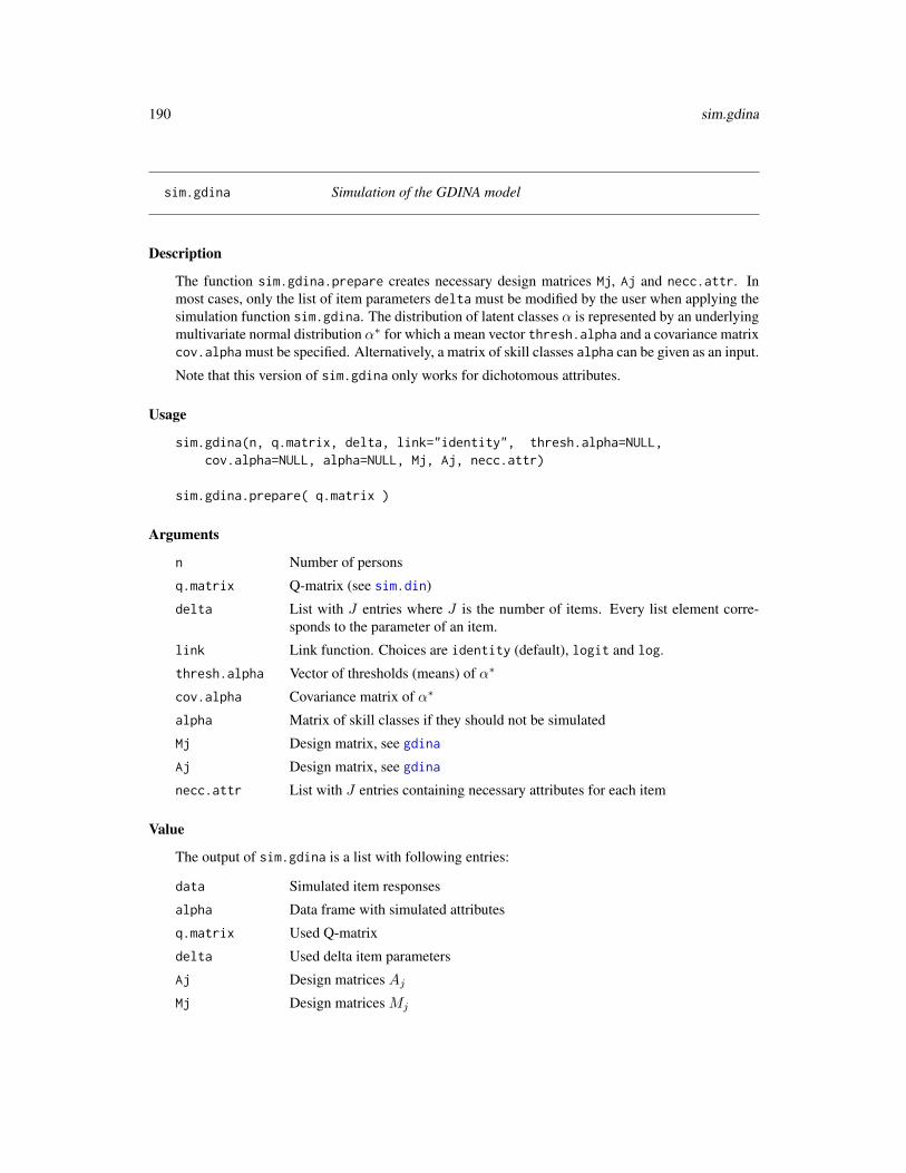
190 sim.gdina

sim.gdina Simulation of the GDINA model

Description

The function sim.gdina.prepare creates necessary design matrices Mj, Aj and necc.attr. Inmost cases, only the list of item parameters delta must be modified by the user when applying thesimulation function sim.gdina. The distribution of latent classes α is represented by an underlyingmultivariate normal distribution α∗ for which a mean vector thresh.alpha and a covariance matrixcov.alpha must be specified. Alternatively, a matrix of skill classes alpha can be given as an input.

Note that this version of sim.gdina only works for dichotomous attributes.

Usage

sim.gdina(n, q.matrix, delta, link="identity", thresh.alpha=NULL,cov.alpha=NULL, alpha=NULL, Mj, Aj, necc.attr)

sim.gdina.prepare( q.matrix )

Arguments

n Number of persons

q.matrix Q-matrix (see sim.din)

delta List with J entries where J is the number of items. Every list element corre-sponds to the parameter of an item.

link Link function. Choices are identity (default), logit and log.

thresh.alpha Vector of thresholds (means) of α∗

cov.alpha Covariance matrix of α∗

alpha Matrix of skill classes if they should not be simulated

Mj Design matrix, see gdina

Aj Design matrix, see gdina

necc.attr List with J entries containing necessary attributes for each item

Value

The output of sim.gdina is a list with following entries:

data Simulated item responses

alpha Data frame with simulated attributes


delta Used delta item parameters

Aj Design matrices AjMj Design matrices Mj

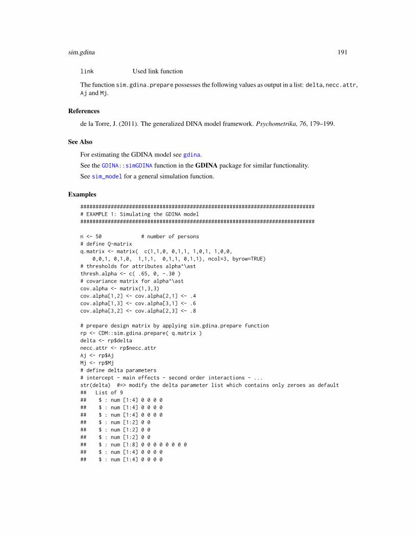
sim.gdina 191

link Used link function

The function sim.gdina.prepare possesses the following values as output in a list: delta, necc.attr,Aj and Mj.

References

de la Torre, J. (2011). The generalized DINA model framework. Psychometrika, 76, 179–199.

See Also

For estimating the GDINA model see gdina.

See the GDINA::simGDINA function in the GDINA package for similar functionality.

See sim_model for a general simulation function.

Examples

############################################################################## EXAMPLE 1: Simulating the GDINA model#############################################################################

n <- 50 # number of persons# define Q-matrixq.matrix <- matrix( c(1,1,0, 0,1,1, 1,0,1, 1,0,0,

0,0,1, 0,1,0, 1,1,1, 0,1,1, 0,1,1), ncol=3, byrow=TRUE)# thresholds for attributes alpha^\astthresh.alpha <- c( .65, 0, -.30 )# covariance matrix for alpha^\astcov.alpha <- matrix(1,3,3)cov.alpha[1,2] <- cov.alpha[2,1] <- .4cov.alpha[1,3] <- cov.alpha[3,1] <- .6cov.alpha[3,2] <- cov.alpha[2,3] <- .8

# prepare design matrix by applying sim.gdina.prepare functionrp <- CDM::sim.gdina.prepare( q.matrix )delta <- rp$deltanecc.attr <- rp$necc.attrAj <- rp$AjMj <- rp$Mj# define delta parameters# intercept - main effects - second order interactions - ...str(delta) #=> modify the delta parameter list which contains only zeroes as default## List of 9## $ : num [1:4] 0 0 0 0## $ : num [1:4] 0 0 0 0## $ : num [1:4] 0 0 0 0## $ : num [1:2] 0 0## $ : num [1:2] 0 0## $ : num [1:2] 0 0## $ : num [1:8] 0 0 0 0 0 0 0 0## $ : num [1:4] 0 0 0 0## $ : num [1:4] 0 0 0 0

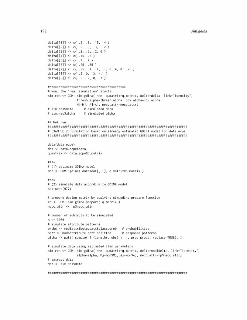
192 sim.gdina

delta[[1]] <- c( .2, .1, .15, .4 )delta[[2]] <- c( .2, .3, .3, -.2 )delta[[3]] <- c( .2, .2, .2, 0 )delta[[4]] <- c( .15, .6 )delta[[5]] <- c( .1, .7 )delta[[6]] <- c( .25, .65 )delta[[7]] <- c( .25, .1, .1, .1, 0, 0, 0, .25 )delta[[8]] <- c( .2, 0, .3, -.1 )delta[[9]] <- c( .2, .2, 0, .3 )

#******************************************# Now, the "real simulation" startssim.res <- CDM::sim.gdina( n=n, q.matrix=q.matrix, delta=delta, link="identity",

thresh.alpha=thresh.alpha, cov.alpha=cov.alpha,Mj=Mj, Aj=Aj, necc.attr=necc.attr)

# sim.res$data # simulated data# sim.res$alpha # simulated alpha

## Not run:############################################################################## EXAMPLE 2: Simulation based on already estimated GDINA model for data.ecpe#############################################################################

data(data.ecpe)dat <- data.ecpe$dataq.matrix <- data.ecpe$q.matrix

#***# (1) estimate GDINA modelmod <- CDM::gdina( data=dat[,-1], q.matrix=q.matrix )

#***# (2) simulate data according to GDINA modelset.seed(977)

# prepare design matrix by applying sim.gdina.prepare functionrp <- CDM::sim.gdina.prepare( q.matrix )necc.attr <- rp$necc.attr

# number of subjects to be simulatedn <- 3000# simulate attribute patternsprobs <- mod$attribute.patt$class.prob # probabilitiespatt <- mod$attribute.patt.splitted # response patternsalpha <- patt[ sample( 1:(length(probs) ), n, prob=probs, replace=TRUE), ]

# simulate data using estimated item parameterssim.res <- CDM::sim.gdina( n=n, q.matrix=q.matrix, delta=mod$delta, link="identity",

alpha=alpha, Mj=mod$Mj, Aj=mod$Aj, necc.attr=rp$necc.attr)# extract datadat <- sim.res$data

#############################################################################

sim_model 193

# EXAMPLE 3: Simulation based on already estimated RRUM model for data.ecpe#############################################################################

dat <- CDM::data.ecpe$dataq.matrix <- CDM::data.ecpe$q.matrix

#***# (1) estimate reduced RUM modelmod <- CDM::gdina( data=dat[,-1], q.matrix=q.matrix, rule="RRUM" )summary(mod)

#***# (2) simulate data according to RRUM modelset.seed(977)

# prepare design matrix by applying sim.gdina.prepare functionrp <- CDM::sim.gdina.prepare( q.matrix )necc.attr <- rp$necc.attr

# number of subjects to be simulatedn <- 5000# simulate attribute patternsprobs <- mod$attribute.patt$class.prob # probabilitiespatt <- mod$attribute.patt.splitted # response patternsalpha <- patt[ sample( 1:(length(probs) ), n, prob=probs, replace=TRUE), ]

# simulate data using estimated item parameterssim.res <- CDM::sim.gdina( n=n, q.matrix=q.matrix, delta=mod$delta, link=mod$link,

alpha=alpha, Mj=mod$Mj, Aj=mod$Aj, necc.attr=rp$necc.attr)# extract datadat <- sim.res$data

## End(Not run)

sim_model Simulate an Item Response Model

Description

Simulates an item response model given a fitted object or input of item response probabilities andskill class probabilities.

Usage

sim_model(object=NULL, irfprob=NULL, theta_index=NULL, prob.theta=NULL,data=NULL, N_sim=NULL )

194 sim_model

Arguments

object Fitted object for which the methods IRT.posterior, and IRT.data are defined.

irfprob Array of item response function values (items × categories × skill classes)

theta_index Skill class index for sampling

prob.theta Skill class probabilities

data Original dataset, only relevant for simulating item response pattern with missingvalues

N_sim Number of subjects to be simulated

Value

List containing elements

dat Simulated item responses

theta Simulated skill classes

theta_index Corresponding indices to theta

Examples

## Not run:############################################################################## EXAMPLE 1: GDINA model simulation#############################################################################

data(sim.dina, package="CDM")data(sim.qmatrix, package="CDM")dat <- sim.dinaQ <- sim.qmatrix

# fit DINA modelmod <- CDM::gdina( dat, q.matrix=Q, rule="DINA")summary(mod)

#** simulate new item responses (N equals observed sample size)dat1 <- CDM::sim_model(mod)

#*** simulate item responses for N=2000 subjectsdat2 <- CDM::sim_model(mod, N_sim=2000)str(dat2)

#*** simulate item responses based on input item response probabilities#*** and theta_indexirfprob <- CDM::IRT.irfprob(mod)prob.theta <- attr(irfprob, "prob.theta")TP <- length(prob.theta)theta_index <- sample(1:TP, size=1000, prob=prob.theta, replace=TRUE )#-- simulatedat3 <- CDM::sim_model(irfprob=irfprob, theta_index=theta_index)str(dat3)

skill.cor 195

## End(Not run)

skill.cor Tetrachoric or Polychoric Correlations between Attributes

Description

This function takes the results of din or gdina and computes tetrachoric or polychoric correlationsbetween attributes (see e.g. Templin & Henson, 2006).

Usage

# tetrachoric correlationsskill.cor(object)

# polychoric correlationsskill.polychor(object, colindex=1)

Arguments

object Object of class din or gdina

colindex Index which can used for group-wise calculation of polychoric correlations

Value


conttable.skills

Bivariate contingency table of all skill pairs

cor.skills Tetrachoric correlation matrix for skill distribution

References

Templin, J., & Henson, R. (2006). Measurement of psychological disorders using cognitive diag-nosis models. Psychological Methods, 11, 287-305.

Examples


# estimate modeld4 <- CDM::din( sim.dino, q.matrix=sim.qmatrix)# compute tetrachoric correlationsCDM::skill.cor(d4)

## estimated tetrachoric correlations## $cor.skills## V1 V2 V3

196 skillspace.approximation

## V1 1.0000000 0.2567718 0.2552958## V2 0.2567718 1.0000000 0.9842188## V3 0.2552958 0.9842188 1.0000000

skillspace.approximation

Skill Space Approximation

Description

This function approximates the skill space withK skills to approximate a (typically high-dimensional)skill space of 2K classes by L classes (L < 2K). The large number of latent classes are representedby underlying continuous latent variables for the dichotomous skills (see George & Robitzsch, 2014,for more details).

Usage

skillspace.approximation(L, K, nmax=5000)

Arguments

L Number of skill classes used for approximation

K Number of skills

nmax Number of quasi-randomly generated skill classes using the QUnif function insfsmisc

Value

A matrix containing skill classes in rows

Note

This function uses the sfsmisc::QUnif function from the sfsmisc package.

References

George, A. C., & Robitzsch, A. (2014). Multiple group cognitive diagnosis models, with an empha-sis on differential item functioning. Psychological Test and Assessment Modeling, 56(4), 405-432.

See Also

See also gdina (Example 9).

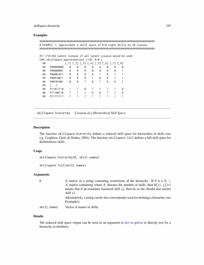
skillspace.hierarchy 197

Examples

############################################################################## EXAMPLE 1: Approximate a skill space of K=8 eight skills by 20 classes#############################################################################

#=> 2^8=256 latent classes if all latent classes would be usedCDM::skillspace.approximation( L=20, K=8 )

## [,1] [,2] [,3] [,4] [,5] [,6] [,7] [,8]## P00000000 0 0 0 0 0 0 0 0## P00000001 0 0 0 0 0 0 0 1## P00001011 0 0 0 0 1 0 1 1## P00010011 0 0 0 1 0 0 1 1## P00101001 0 0 1 0 1 0 0 1## [...]## P11011110 1 1 0 1 1 1 1 0## P11100110 1 1 1 0 0 1 1 0## P11111111 1 1 1 1 1 1 1 1

skillspace.hierarchy Creation of a Hierarchical Skill Space

Description

The function skillspace.hierarchy defines a reduced skill space for hierarchies in skills (seee.g. Leighton, Gierl, & Hunka, 2004). The function skillspace.full defines a full skill space fordichotomous skills.

Usage

skillspace.hierarchy(B, skill.names)

skillspace.full(skill.names)

Arguments

B A matrix or a string containing restrictions of the hierarchy. If B is a K ×K matrix containing where K denotes the number of skills, then B[ii,jj]=1means that if an examinee mastered skill jj, then he or she should also masterskill ii.Alternatively, a string can be also conveniently used for defining a hierarchy (seeExamples).

skill.names Vector of names in skills

Details

The reduced skill space output can be used as an argument in din or gdina to directly test for ahierarchy in attributes.

198 skillspace.hierarchy

Value


R Reachability matrixskillspace.reduced

Reduced skill space fulfilling the specified hierarchyskillspace.complete

Complete skill spacezeroprob.skillclasses

Indices of skill patterns in skillspace.complete which were removed fordefining skillspace.reduced

References

Leighton, J. P., Gierl, M. J., & Hunka, S. M. (2004). The attribute hierarchy method for cognitiveassessment: A variation on Tatsuoka’s rule space approach. Journal of Educational Measurement,41, 205-237.

See Also

See din (Example 6) for an application of skillspace.hierarchy for model comparisons.

See the GDINA::att.structure function in the GDINA package for similar functionality.

Examples

############################################################################## EXAMPLE 1: Toy example with 3 skills#############################################################################

K <- 3 # number of skillsskill.names <- paste0("A", 1:K ) # names of skills

# create a zero matrix for hierarchy definitionB0 <- 0*diag(K)rownames(B0) <- colnames(B0) <- skill.names

#*** Model 1: A1 > A2 > A3B <- B0B[1,2] <- 1 # A1 > A2B[2,3] <- 1 # A2 > A3

sp1 <- CDM::skillspace.hierarchy( B=B, skill.names=skill.names )sp1$skillspace.reduced

## A1 A2 A3## 1 0 0 0## 2 1 0 0## 4 1 1 0## 8 1 1 1

#*** Model 2: A1 > A2 and A1 > A3

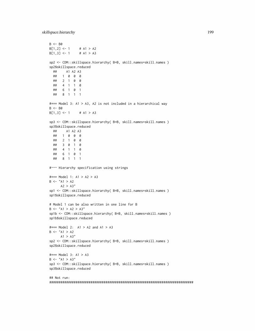
skillspace.hierarchy 199

B <- B0B[1,2] <- 1 # A1 > A2B[1,3] <- 1 # A1 > A3


## A1 A2 A3## 1 0 0 0## 2 1 0 0## 4 1 1 0## 6 1 0 1## 8 1 1 1

#*** Model 3: A1 > A3, A2 is not included in a hierarchical wayB <- B0B[1,3] <- 1 # A1 > A3


## A1 A2 A3## 1 0 0 0## 2 1 0 0## 3 0 1 0## 4 1 1 0## 6 1 0 1## 8 1 1 1

#~~~ Hierarchy specification using strings

#*** Model 1: A1 > A2 > A3B <- "A1 > A2

A2 > A3"sp1 <- CDM::skillspace.hierarchy( B=B, skill.names=skill.names )sp1$skillspace.reduced

# Model 1 can be also written in one line for BB <- "A1 > A2 > A3"sp1b <- CDM::skillspace.hierarchy( B=B, skill.names=skill.names )sp1b$skillspace.reduced

#*** Model 2: A1 > A2 and A1 > A3B <- "A1 > A2

A1 > A3"sp2 <- CDM::skillspace.hierarchy( B=B, skill.names=skill.names )sp2$skillspace.reduced

#*** Model 3: A1 > A3B <- "A1 > A3"sp3 <- CDM::skillspace.hierarchy( B=B, skill.names=skill.names )sp3$skillspace.reduced

## Not run:#############################################################################

200 slca

# EXAMPLE 2: Examples from Leighton et al. (2004): Fig. 1 (p. 210)#############################################################################

skill.names <- paste0("A",1:6) # 6 skills

#*** Model 1: Linear hierarchy (A)B <- "A1 > A2 > A3 > A4 > A5 > A6"sp1 <- CDM::skillspace.hierarchy( B=B, skill.names=skill.names )sp1$skillspace.reduced

#*** Model 2: Convergent hierarchy (B)B <- "A1 > A2 > A3

A2 > A4A3 > A5 > A6A4 > A5 > A6"


#*** Model 3: Divergent hierarchy (C)B <- "A1 > A2 > A3

A1 > A4 > A5A1 > A4 > A6"


#*** Model 4: Unstructured hierarchy (D)B <- "A1 > A2 \n A1 > A3 \n A1 > A4 \n A1 > A5 \n A1 > A6"# This specification of B is equivalent to writing separate lines:# B <- "A1 > A2# A1 > A3# A1 > A4# A1 > A5# A1 > A6"sp4 <- CDM::skillspace.hierarchy( B=B, skill.names=skill.names )sp4$skillspace.reduced

## End(Not run)

slca Structured Latent Class Analysis (SLCA)

Description

This function implements a structured latent class model for polytomous item responses (Formann,1985, 1992). Lasso estimation for the item parameters is included (Chen, Liu, Xu & Ying, 2015;Chen, Li, Liu & Ying, 2017; Sun, Chen, Liu, Ying & Xin, 2016).

Usage

slca(data, group=NULL, weights=rep(1, nrow(data)), Xdes,

slca 201

Xlambda.init=NULL, Xlambda.fixed=NULL, Xlambda.constr.V=NULL,Xlambda.constr.c=NULL, delta.designmatrix=NULL,delta.init=NULL, delta.fixed=NULL, delta.linkfct="log",Xlambda_positive=NULL, regular_type="lasso", regular_lam=0, regular_w=NULL,regular_n=nrow(data), maxiter=1000, conv=1e-5, globconv=1e-5, msteps=10,convM=5e-04, decrease.increments=FALSE, oldfac=0, dampening_factor=1.01,seed=NULL, progress=TRUE, PEM=TRUE, PEM_itermax=maxiter, ...)

## S3 method for class 'slca'summary(object, file=NULL, ...)

## S3 method for class 'slca'print(x, ...)

## S3 method for class 'slca'plot(x, group=1, ... )

Arguments

data Matrix of polytomous item responses

group Optional vector of group identifiers. For plot.slca it is a single integer groupidentified.

weights Optional vector of sample weights

Xdes Design matrix for xijh with qihjv entries. Therefore, it must be an array withfour dimensions referring to items (i), categories (h), latent classes (j) and λparameters (v).

Xlambda.init Initial λx parameters

Xlambda.fixed Fixed λx parameters. These must be provided by a matrix with two columns:1st column – Parameter index, 2nd column: Fixed value.

Xlambda.constr.V

A design matrix for linear restrictions of the form Vxλx = cx for the λx param-eter.

Xlambda.constr.c

A vector for the linear restriction Vxλx = cx of the λx parameter.delta.designmatrix

Design matrix for delta parameters δ parameterizing the latent class distributionby log-linear smoothing (Xu & von Davier, 2008)

delta.init Initial δ parameters

delta.fixed Fixed δ parameters. This must be a matrix with three columns: 1st column:Parameter index, 2nd column: Group index, 3rd column: Fixed value

delta.linkfct Link function for skill space reduction. This can be the log-linear link (log) orthe logistic link function (logit).

Xlambda_positive

Optional vector of logical indicating which elements ofλx should be constrainedto be positive.

202 slca

regular_type Regularization method which can be lasso, scad or mcp. See gdina for moreinformation and references.

regular_lam Numeric. Regularization parameter

regular_w Vector for weighting the regularization penalty

regular_n Vector of regularization factor. This will be typically the sample size.


conv Convergence criterion for item parameters and distribution parameters

globconv Global deviance convergence criterion

msteps Maximum number of M steps in estimating b and a item parameters. The defaultis to use 4 M steps.

convM Convergence criterion in M stepdecrease.increments

Should in the M step the increments of a and b parameters decrease during itera-tions? The default is FALSE. If there is an increase in deviance during estimation,setting decrease.increments to TRUE is recommended.

oldfac Factor f between 0 and 1 to control convergence behavior. If xt denotes theestimated parameter in iteration t, then the regularized estimate x∗t is obtainedby x∗t = fxt−1 +(1−f)xt. Therefore, values of oldfac near to one only allowfor small changes in estimated parameters from in succeeding iterations.

dampening_factor

Factor larger than one defining the specified decrease in decrements in iterations.

seed Simulation seed for initial parameters. The default of NULL corresponds to arandom seed.




object A required object of class slca


x A required object of class slca


Details

The structured latent class model allows for general constraints of items i in categories h and classesj. The item response model is

P (Xi = h|j) =exp(xihj)∑l exp(xilj)

with linear constraints on the class specific probabilities

xihj =∑v

qihjvλxv

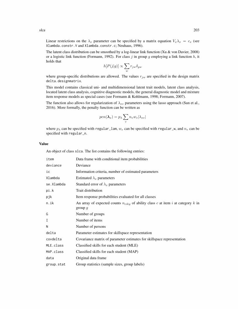
slca 203

Linear restrictions on the λx parameter can be specified by a matrix equation Vxλx = cx (seeXlambda.constr.V and Xlambda.constr.c; Neuhaus, 1996).

The latent class distribution can be smoothed by a log-linear link function (Xu & von Davier, 2008)or a logistic link function (Formann, 1992). For class j in group g employing a link function h, itholds that

h[P (j|g)] ∝∑w

rjwδgw

where group-specific distributions are allowed. The values rjw are specified in the design matrixdelta.designmatrix.

This model contains classical uni- and multidimensional latent trait models, latent class analysis,located latent class analysis, cognitive diagnostic models, the general diagnostic model and mixtureitem response models as special cases (see Formann & Kohlmann, 1998; Formann, 2007).

The function also allows for regularization of λxv parameters using the lasso approach (Sun et al.,2016). More formally, the penalty function can be written as

pen(λx) = pλ∑v

nvwv|λxv|

where pλ can be specified with regular_lam, wv can be specified with regular_w, and nv can bespecified with regular_n.

Value

An object of class slca. The list contains the following entries:

item Data frame with conditional item probabilities

deviance Deviance

ic Information criteria, number of estimated parameters

Xlambda Estimated λx parameters

se.Xlambda Standard error of λx parameters

pi.k Trait distribution

pjk Item response probabilities evaluated for all classes

n.ik An array of expected counts ncikg of ability class c at item i at category k ingroup g

G Number of groups

I Number of items

N Number of persons

delta Parameter estimates for skillspace representation

covdelta Covariance matrix of parameter estimates for skillspace representation

MLE.class Classified skills for each student (MLE)

MAP.class Classified skills for each student (MAP)

data Original data frame


204 slca

p.xi.aj Individual likelihood


K.item Maximal category per item

time Info about computation time

skillspace Used skillspace parametrization


seed.used Used simulation seed

Xlambda.init Used initial lambda parameters

delta.init Used initial delta parameters


Note

If some items have differing number of categories, appropriate class probabilities in non-existingcategories per items can be practically set to zero by loading an item for all skill classes on a fixedλx parameter of a small number, e.g. -999.

The implementation of the model builds on pieces work of Anton Formann. See http://www.antonformann.at/ for more information.

References


Chen, Y., Liu, J., Xu, G., & Ying, Z. (2015). Statistical analysis of Q-matrix based diagnosticclassification models. Journal of the American Statistical Association, 110, 850-866.


Formann, A. K. (1985). Constrained latent class models: Theory and applications. British Journalof Mathematical and Statistical Psychology, 38, 87-111.

Formann, A. K. (1992). Linear logistic latent class analysis for polytomous data. Journal of theAmerican Statistical Association, 87, 476-486.

Formann, A. K. (2007). (Almost) Equivalence between conditional and mixture maximum likeli-hood estimates for some models of the Rasch type. In M. von Davier & C. H. Carstensen (Eds.),Multivariate and mixture distribution Rasch models (pp. 177-189). New York: Springer.

Formann, A. K., & Kohlmann, T. (1998). Structural latent class models. Sociological Methods &Research, 26, 530-565.

Neuhaus, W. (1996). Optimal estimation under linear constraints. Astin Bulletin, 26, 233-245.

Sun, J., Chen, Y., Liu, J., Ying, Z., & Xin, T. (2016). Latent variable selection for multidimensionalitem response theory models via L1 regularization. Psychometrika, 81(4), 921-939.


http://www.antonformann.at/

http://www.antonformann.at/

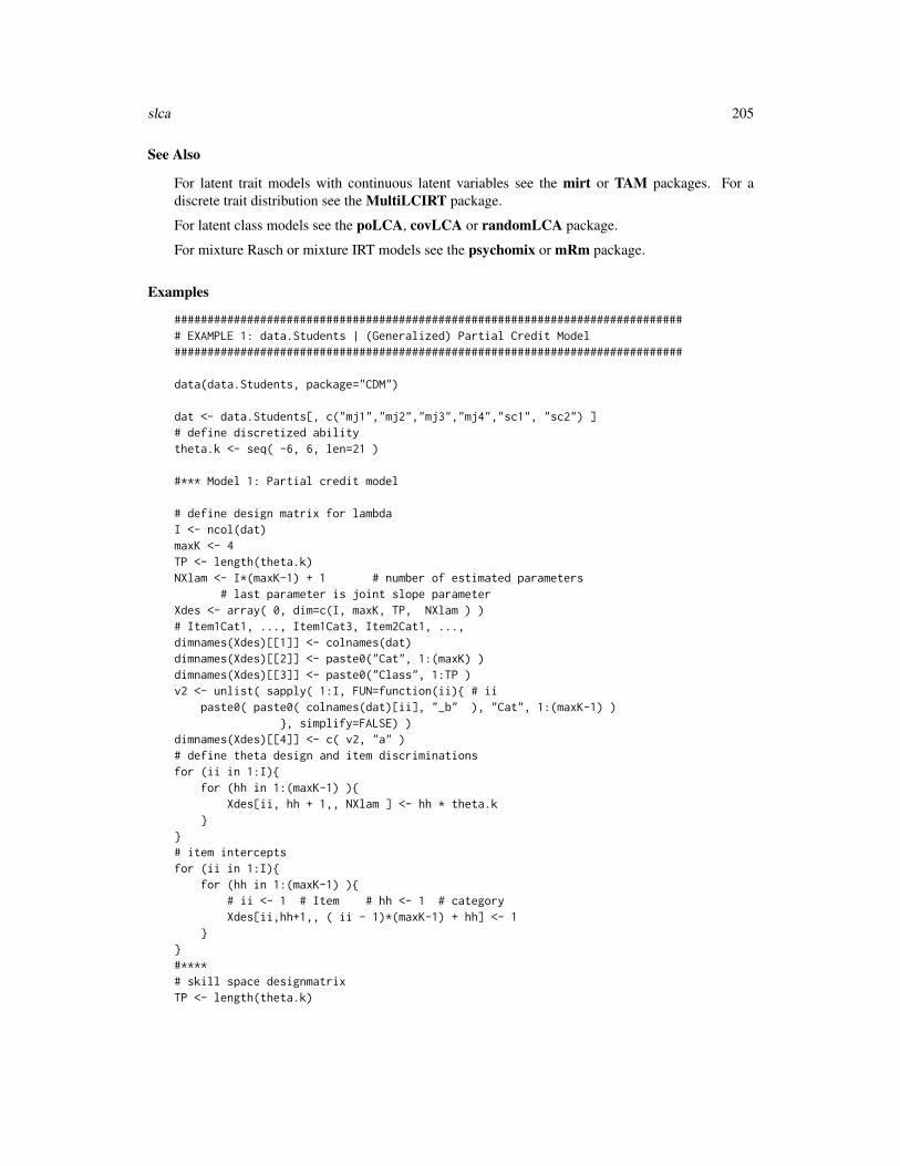
slca 205

See Also

For latent trait models with continuous latent variables see the mirt or TAM packages. For adiscrete trait distribution see the MultiLCIRT package.

For latent class models see the poLCA, covLCA or randomLCA package.

For mixture Rasch or mixture IRT models see the psychomix or mRm package.

Examples

############################################################################## EXAMPLE 1: data.Students | (Generalized) Partial Credit Model#############################################################################

data(data.Students, package="CDM")

dat <- data.Students[, c("mj1","mj2","mj3","mj4","sc1", "sc2") ]# define discretized abilitytheta.k <- seq( -6, 6, len=21 )

#*** Model 1: Partial credit model

# define design matrix for lambdaI <- ncol(dat)maxK <- 4TP <- length(theta.k)NXlam <- I*(maxK-1) + 1 # number of estimated parameters

# last parameter is joint slope parameterXdes <- array( 0, dim=c(I, maxK, TP, NXlam ) )# Item1Cat1, ..., Item1Cat3, Item2Cat1, ...,dimnames(Xdes)[[1]] <- colnames(dat)dimnames(Xdes)[[2]] <- paste0("Cat", 1:(maxK) )dimnames(Xdes)[[3]] <- paste0("Class", 1:TP )v2 <- unlist( sapply( 1:I, FUN=function(ii){ # ii

paste0( paste0( colnames(dat)[ii], "_b" ), "Cat", 1:(maxK-1) )}, simplify=FALSE) )

dimnames(Xdes)[[4]] <- c( v2, "a" )# define theta design and item discriminationsfor (ii in 1:I){

for (hh in 1:(maxK-1) ){Xdes[ii, hh + 1,, NXlam ] <- hh * theta.k

}}# item interceptsfor (ii in 1:I){

for (hh in 1:(maxK-1) ){# ii <- 1 # Item # hh <- 1 # categoryXdes[ii,hh+1,, ( ii - 1)*(maxK-1) + hh] <- 1

}}#****# skill space designmatrixTP <- length(theta.k)

206 slca

w1 <- stats::dnorm(theta.k)w1 <- w1 / sum(w1)delta.designmatrix <- matrix( 1, nrow=TP, ncol=1 )delta.designmatrix[,1] <- log(w1)

# initial lambda parametersXlambda.init <- c( stats::rnorm( dim(Xdes)[[4]] - 1 ), 1 )# fixed delta parameterdelta.fixed <- cbind( 1, 1,1 )

# estimate modelmod1 <- CDM::slca( dat, Xdes=Xdes, delta.designmatrix=delta.designmatrix,

Xlambda.init=Xlambda.init, delta.fixed=delta.fixed )summary(mod1)plot(mod1, cex.names=.7 )

## Not run:#*** Model 2: Partial credit model with some parameter constraints# fixed lambda parametersXlambda.fixed <- cbind( c(1,19), c(3.2,1.52 ) )# 1st parameter=3.2# 19th parameter=1.52 (joint item slope)mod2 <- CDM::slca( dat, Xdes=Xdes, delta.designmatrix=delta.designmatrix,

delta.init=delta.init, Xlambda.init=Xlambda.init, delta.fixed=delta.fixed,Xlambda.fixed=Xlambda.fixed, maxiter=70 )

#*** Model 3: Partial credit model with non-normal distributionXlambda.fixed <- cbind( c(1,19), c(3.2,1) ) # fix item slope to onedelta.designmatrix <- cbind( 1, theta.k, theta.k^2, theta.k^3 )mod3 <- CDM::slca( dat, Xdes=Xdes, delta.designmatrix=delta.designmatrix,

Xlambda.fixed=Xlambda.fixed, maxiter=200 )summary(mod3)

# non-normal distribution with convergence regularizing factor oldfacmod3a <- CDM::slca( dat, Xdes=Xdes, delta.designmatrix=delta.designmatrix,

Xlambda.fixed=Xlambda.fixed, maxiter=500, oldfac=.95 )summary(mod3a)

#*** Model 4: Generalized Partial Credit Model

# estimate generalized partial credit model without restrictions on trait# distribution and item parameters to ensure better convergence behavior# Note that two parameters are not identifiable and information criteria# have to be adapted.

#---# define design matrix for lambdaI <- ncol(dat)maxK <- 4TP <- length(theta.k)NXlam <- I*(maxK-1) + I # number of estimated parametersXdes <- array( 0, dim=c(I, maxK, TP, NXlam ) )# Item1Cat1, ..., Item1Cat3, Item2Cat1, ...,

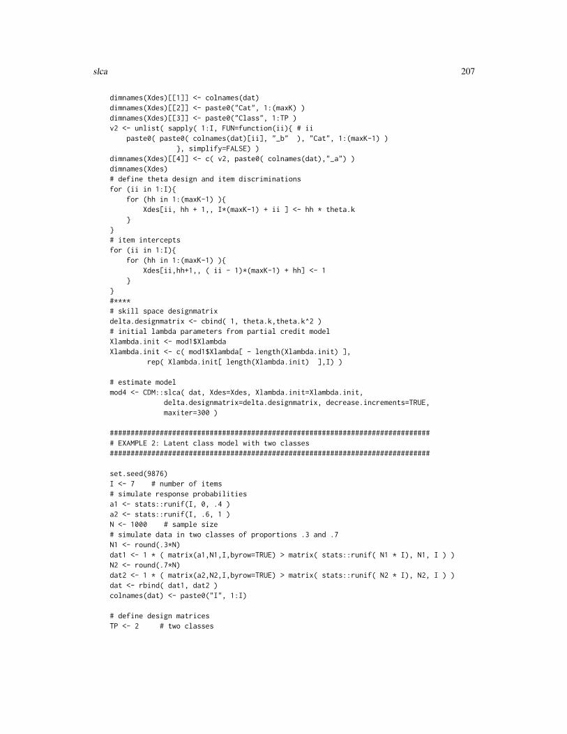
slca 207

dimnames(Xdes)[[1]] <- colnames(dat)dimnames(Xdes)[[2]] <- paste0("Cat", 1:(maxK) )dimnames(Xdes)[[3]] <- paste0("Class", 1:TP )v2 <- unlist( sapply( 1:I, FUN=function(ii){ # ii

paste0( paste0( colnames(dat)[ii], "_b" ), "Cat", 1:(maxK-1) )}, simplify=FALSE) )

dimnames(Xdes)[[4]] <- c( v2, paste0( colnames(dat),"_a") )dimnames(Xdes)# define theta design and item discriminationsfor (ii in 1:I){

for (hh in 1:(maxK-1) ){Xdes[ii, hh + 1,, I*(maxK-1) + ii ] <- hh * theta.k

}}# item interceptsfor (ii in 1:I){

for (hh in 1:(maxK-1) ){Xdes[ii,hh+1,, ( ii - 1)*(maxK-1) + hh] <- 1

}}#****# skill space designmatrixdelta.designmatrix <- cbind( 1, theta.k,theta.k^2 )# initial lambda parameters from partial credit modelXlambda.init <- mod1$XlambdaXlambda.init <- c( mod1$Xlambda[ - length(Xlambda.init) ],

rep( Xlambda.init[ length(Xlambda.init) ],I) )

# estimate modelmod4 <- CDM::slca( dat, Xdes=Xdes, Xlambda.init=Xlambda.init,

delta.designmatrix=delta.designmatrix, decrease.increments=TRUE,maxiter=300 )

############################################################################## EXAMPLE 2: Latent class model with two classes#############################################################################

set.seed(9876)I <- 7 # number of items# simulate response probabilitiesa1 <- stats::runif(I, 0, .4 )a2 <- stats::runif(I, .6, 1 )N <- 1000 # sample size# simulate data in two classes of proportions .3 and .7N1 <- round(.3*N)dat1 <- 1 * ( matrix(a1,N1,I,byrow=TRUE) > matrix( stats::runif( N1 * I), N1, I ) )N2 <- round(.7*N)dat2 <- 1 * ( matrix(a2,N2,I,byrow=TRUE) > matrix( stats::runif( N2 * I), N2, I ) )dat <- rbind( dat1, dat2 )colnames(dat) <- paste0("I", 1:I)

# define design matricesTP <- 2 # two classes

208 slca

# The idea is that latent classes refer to two different "dimensions".# Items load on latent class indicators 1 and 2, see below.Xdes <- array(0, dim=c(I,2,2,2*I) )items <- colnames(dat)dimnames(Xdes)[[4]] <- c(paste0( colnames(dat), "Class", 1),

paste0( colnames(dat), "Class", 2) )# items, categories, classes, parameters

# probabilities for correct solutionfor (ii in 1:I){

Xdes[ ii, 2, 1, ii ] <- 1 # probabilities class 1Xdes[ ii, 2, 2, ii+I ] <- 1 # probabilities class 2

}# estimate modelmod1 <- CDM::slca( dat, Xdes=Xdes )summary(mod1)

############################################################################## EXAMPLE 3: Mixed Rasch model with two classes#############################################################################

set.seed(987)library(sirt)# simulate two latent classes of Rasch populationsI <- 15 # 6 itemsb1 <- seq( -1.5, 1.5, len=I) # difficulties latent class 1b2 <- b1 # difficulties latent class 2b2[ c(4,7, 9, 11, 12, 13) ] <- c(1, -.5, -.5, .33, .33, -.66 )N <- 3000 # number of personswgt <- .25 # class probability for class 1# class 1dat1 <- sirt::sim.raschtype( stats::rnorm( wgt*N ), b1 )# class 2dat2 <- sirt::sim.raschtype( stats::rnorm( (1-wgt)*N, mean=1, sd=1.7), b2 )dat <- rbind( dat1, dat2 )# theta gridtheta.k <- seq( -5, 5, len=9 )TP <- length(theta.k)

#*** Model 1: Rasch model with normal distributionmaxK <- 2NXlam <- I +1Xdes <- array( 0, dim=c(I, maxK, TP, NXlam ) )dimnames(Xdes)[[1]] <- colnames(dat)dimnames(Xdes)[[2]] <- paste0("Cat", 1:(maxK) )dimnames(Xdes)[[4]] <- c( paste0( "b_", colnames(dat)[1:I] ), "a" )# define item difficultiesfor (ii in 1:I){

Xdes[ii, 2,, ii ] <- -1}# theta designfor (tt in 1:TP){

Xdes[1:I, 2, tt, I + 1] <- theta.k[tt]}

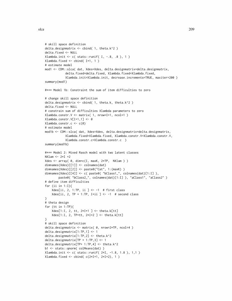
slca 209

# skill space definitiondelta.designmatrix <- cbind( 1, theta.k^2 )delta.fixed <- NULLXlambda.init <- c( stats::runif( I, -.8, .8 ), 1 )Xlambda.fixed <- cbind( I+1, 1 )# estimate modelmod1 <- CDM::slca( dat, Xdes=Xdes, delta.designmatrix=delta.designmatrix,

delta.fixed=delta.fixed, Xlambda.fixed=Xlambda.fixed,Xlambda.init=Xlambda.init, decrease.increments=TRUE, maxiter=200 )

summary(mod1)

#*** Model 1b: Constraint the sum of item difficulties to zero

# change skill space definitiondelta.designmatrix <- cbind( 1, theta.k, theta.k^2 )delta.fixed <- NULL# constrain sum of difficulties Xlambda parameters to zeroXlambda.constr.V <- matrix( 1, nrow=I+1, ncol=1 )Xlambda.constr.V[I+1,1] <- 0Xlambda.constr.c <- c(0)# estimate modelmod1b <- CDM::slca( dat, Xdes=Xdes, delta.designmatrix=delta.designmatrix,

Xlambda.fixed=Xlambda.fixed, Xlambda.constr.V=Xlambda.constr.V,Xlambda.constr.c=Xlambda.constr.c )

summary(mod1b)

#*** Model 2: Mixed Rasch model with two latent classesNXlam <- 2*I +2Xdes <- array( 0, dim=c(I, maxK, 2*TP, NXlam ) )dimnames(Xdes)[[1]] <- colnames(dat)dimnames(Xdes)[[2]] <- paste0("Cat", 1:(maxK) )dimnames(Xdes)[[4]] <- c( paste0( "bClass1_", colnames(dat)[1:I] ),

paste0( "bClass2_", colnames(dat)[1:I] ), "aClass1", "aClass2" )# define item difficultiesfor (ii in 1:I){

Xdes[ii, 2, 1:TP, ii ] <- -1 # first classXdes[ii, 2, TP + 1:TP, I+ii ] <- -1 # second class

}# theta designfor (tt in 1:TP){

Xdes[1:I, 2, tt, 2*I+1 ] <- theta.k[tt]Xdes[1:I, 2, TP+tt, 2*I+2 ] <- theta.k[tt]

}# skill space definitiondelta.designmatrix <- matrix( 0, nrow=2*TP, ncol=4 )delta.designmatrix[1:TP,1] <- 1delta.designmatrix[1:TP,2] <- theta.k^2delta.designmatrix[TP + 1:TP,3] <- 1delta.designmatrix[TP+ 1:TP,4] <- theta.k^2b1 <- stats::qnorm( colMeans(dat) )Xlambda.init <- c( stats::runif( 2*I, -1.8, 1.8 ), 1,1 )Xlambda.fixed <- cbind( c(2*I+1, 2*I+2), 1 )

210 slca

# estimate modelmod2 <- CDM::slca( dat, Xdes=Xdes, delta.designmatrix=delta.designmatrix,

Xlambda.fixed=Xlambda.fixed, decrease.increments=TRUE,Xlambda.init=Xlambda.init, maxiter=1000 )

summary(mod2)summary(mod1)# latent class proportionsstats::aggregate( mod2$pi.k, list( rep(1:2, each=TP)), sum )

#*** Model 2b: Different parametrization with sum constraint on item difficulties

# skill space definitiondelta.designmatrix <- matrix( 0, nrow=2*TP, ncol=6 )delta.designmatrix[1:TP,1] <- 1delta.designmatrix[1:TP,2] <- theta.kdelta.designmatrix[1:TP,3] <- theta.k^2delta.designmatrix[TP+ 1:TP,4] <- 1delta.designmatrix[TP+ 1:TP,5] <- theta.kdelta.designmatrix[TP+ 1:TP,6] <- theta.k^2Xlambda.fixed <- cbind( c(2*I+1,2*I+2), c(1,1) )b1 <- stats::qnorm( colMeans( dat ) )Xlambda.init <- c( b1, b1 + stats::runif(I, -1, 1 ), 1, 1 )# constraints on item difficultiesXlambda.constr.V <- matrix( 0, nrow=NXlam, ncol=2)Xlambda.constr.V[1:I, 1 ] <- 1Xlambda.constr.V[I + 1:I, 2 ] <- 1Xlambda.constr.c <- c(0,0)# estimate modelmod2b <- CDM::slca( dat, Xdes=Xdes, delta.designmatrix=delta.designmatrix,

Xlambda.fixed=Xlambda.fixed, Xlambda.init=Xlambda.init,Xlambda.constr.V=Xlambda.constr.V, Xlambda.constr.c=Xlambda.constr.c,decrease.increments=TRUE, maxiter=1000 )

summary(mod2b)stats::aggregate( mod2b$pi.k, list( rep(1:2, each=TP)), sum )

#*** Model 2c: Estimation with mRm packagelibrary(mRm)mod2c <- mRm::mrm(data.matrix=dat, cl=2)plot(mod2c)print(mod2c)

#*** Model 2d: Estimation with psychomix packagelibrary(psychomix)mod2d <- psychomix::raschmix(data=dat, k=2, verbose=TRUE )summary(mod2d)plot(mod2d)

############################################################################## EXAMPLE 4: Located latent class model, Rasch model#############################################################################

set.seed(487)library(sirt)

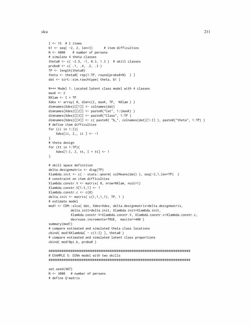
slca 211

I <- 15 # I itemsb1 <- seq( -2, 2, len=I) # item difficultiesN <- 4000 # number of persons# simulate 4 theta classestheta0 <- c( -2.5, -1, 0.3, 1.3 ) # skill classesprobs0 <- c( .1, .4, .2, .3 )TP <- length(theta0)theta <- theta0[ rep(1:TP, round(probs0*N) ) ]dat <- sirt::sim.raschtype( theta, b1 )

#*** Model 1: Located latent class model with 4 classesmaxK <- 2NXlam <- I + TPXdes <- array( 0, dim=c(I, maxK, TP, NXlam ) )dimnames(Xdes)[[1]] <- colnames(dat)dimnames(Xdes)[[2]] <- paste0("Cat", 1:(maxK) )dimnames(Xdes)[[3]] <- paste0("Class", 1:TP )dimnames(Xdes)[[4]] <- c( paste0( "b_", colnames(dat)[1:I] ), paste0("theta", 1:TP) )# define item difficultiesfor (ii in 1:I){

Xdes[ii, 2,, ii ] <- -1}# theta designfor (tt in 1:TP){

Xdes[1:I, 2, tt, I + tt] <- 1}

# skill space definitiondelta.designmatrix <- diag(TP)Xlambda.init <- c( - stats::qnorm( colMeans(dat) ), seq(-2,1,len=TP) )# constraint on item difficultiesXlambda.constr.V <- matrix( 0, nrow=NXlam, ncol=1)Xlambda.constr.V[1:I,1] <- 1Xlambda.constr.c <- c(0)delta.init <- matrix( c(1,1,1,1), TP, 1 )# estimate modelmod1 <- CDM::slca( dat, Xdes=Xdes, delta.designmatrix=delta.designmatrix,

delta.init=delta.init, Xlambda.init=Xlambda.init,Xlambda.constr.V=Xlambda.constr.V, Xlambda.constr.c=Xlambda.constr.c,decrease.increments=TRUE, maxiter=400 )

summary(mod1)# compare estimated and simulated theta class locationscbind( mod1$Xlambda[ - c(1:I) ], theta0 )# compare estimated and simulated latent class proportionscbind( mod1$pi.k, probs0 )

############################################################################## EXAMPLE 5: DINA model with two skills#############################################################################

set.seed(487)N <- 3000 # number of persons# define Q-matrix

212 slca

I <- 9 # 9 itemsNS <- 2 # 2 skillsTP <- 4 # number of skill classesQ <- scan( nlines=3)

1 0 1 0 1 00 1 0 1 0 11 1 1 1 1 1

Q <- matrix(Q, I, ncol=NS,byrow=TRUE)# define skill distributionalpha0 <- matrix( c(0,0,1,0,0,1,1,1), nrow=4,ncol=2,byrow=TRUE)prob0 <- c( .2, .4, .1, .3 )alpha <- alpha0[ rep( 1:TP, prob0*N),]# define guessing and slipping parametersguess <- round( stats::runif(I, 0, .4 ), 2 )slip <- round( stats::runif(I, 0, .3 ), 2 )# simulate data according to the DINA modeldat <- CDM::sim.din( q.matrix=Q, alpha=alpha, slip=slip, guess=guess )$dat

# define Xlambda design matrixmaxK <- 2NXlam <- 2*IXdes <- array( 0, dim=c(I, maxK, TP, NXlam ) )dimnames(Xdes)[[1]] <- colnames(dat)dimnames(Xdes)[[2]] <- paste0("Cat", 1:(maxK) )dimnames(Xdes)[[3]] <- c("S00","S10","S01","S11")dimnames(Xdes)[[4]] <- c( paste0("guess",1:I ), paste0( "antislip", 1:I ) )dimnames(Xdes)# define item difficultiesfor (ii in 1:I){

# define latent responseslatresp <- 1*( alpha0 %*% Q[ii,]==sum(Q[ii,]) )[,1]# model slipping parametersXdes[ii, 2, latresp==1, I+ii ] <- 1# guessing parametersXdes[ii, 2, latresp==0, ii ] <- 1

}Xdes[1,2,,]Xdes[7,2,,]# skill space definitiondelta.designmatrix <- diag(TP)Xlambda.init <- c( rep( stats::qlogis( .2 ), I ), rep( stats::qlogis( .8 ), I ) )

# estimate DINA model with slca functionmod1 <- CDM::slca( dat, Xdes=Xdes, delta.designmatrix=delta.designmatrix,

Xlambda.init=Xlambda.init, decrease.increments=TRUE, maxiter=400 )summary(mod1)

# compare estimated and simulated latent class proportionscbind( mod1$pi.k, probs0 )# compare estimated and simulated guessing parameterscbind( mod1$pjk[1,,2], guess )# compare estimated and simulated slipping parameterscbind( 1 - mod1$pjk[4,,2], slip )

slca 213

############################################################################## EXAMPLE 6: Investigating differential item functioning in Rasch models# with regularization#############################################################################

#---- simulate dataset.seed(987)N <- 1000 # number of persons in a groupI <- 20 # number of items#* population parameters of two groupsmu1 <- 0mu2 <- .6sd1 <- 1.4sd2 <- 1# item difficultiesb <- seq( -1.1, 1.1, len=I )# define some DIF effectsdif <- rep(0,I)dif[ c(3,6,9,12)] <- c( .6, -1, .75, -.35 )print(dif)#* simulate datasetsdat1 <- sirt::sim.raschtype( rnorm(N, mean=mu1, sd=sd1), b=b - dif /2 )colnames(dat1) <- paste0("I", 1:I, "_G1")dat2 <- sirt::sim.raschtype( rnorm(N, mean=mu2, sd=sd2), b=b + dif /2 )colnames(dat2) <- paste0("I", 1:I, "_G2")dat <- CDM::CDM_rbind_fill( dat1, dat2 )dat <- data.frame( "group"=rep(1:2, each=N), dat )

#-- nodes for distributiontheta.k <- seq(-4, 4, len=11)# define design matrix for lambdanitems <- ncol(dat) - 1maxK <- 2TP <- length(theta.k)NXlam <- 2*I + 1Xdes <- array( 0, dim=c( nitems, maxK, TP, NXlam ) )dimnames(Xdes)[[1]] <- colnames(dat)[-1]dimnames(Xdes)[[2]] <- paste0("Cat", 0:(maxK-1) )dimnames(Xdes)[[3]] <- paste0("Theta", 1:TP )dimnames(Xdes)[[4]] <- c( paste0("b", 1:I ), paste0("dif", 1:I ), "const" )# define theta designfor (ii in 1:nitems){

Xdes[ii,2,,NXlam ] <- theta.k}# item intercepts and DIF effectsfor (ii in 1:I){

Xdes[c(ii,ii+I),2,, ii ] <- -1Xdes[ii,2,,ii+I] <- - 1/2Xdes[ii+I,2,,ii+I] <- 1/2

}#--- skill space designmatrixTP <- length(theta.k)

214 summary.din

w1 <- stats::dnorm(theta.k)w1 <- w1 / sum(w1)delta.designmatrix <- matrix( 1, nrow=TP, ncol=2 )delta.designmatrix[,2] <- log(w1)

# fixed lambda parametersXlambda.fixed <- cbind(NXlam, 1 )# initial Xlambda parametersdif_sim <- 0*stats::rnorm(I, sd=.2)Xlambda.init <- c( - stats::qnorm( colMeans(dat1) ), dif_sim, 1 )

# delta.fixeddelta.fixed <- cbind( 1, 1, 0 )# regularization parameterregular_lam <- .2# weighting vector: regularize only DIF effectsregular_w <- c( rep(0,I), rep(1,I), 0 )

#--- estimation model with scad penaltymod1 <- CDM::slca( dat[,-1], group=dat$group, Xdes=Xdes,

delta.designmatrix=delta.designmatrix, regular_type="scad",Xlambda.init=Xlambda.init, delta.fixed=delta.fixed, Xlambda.fixed=Xlambda.fixed,

regular_lam=regular_lam, regular_w=regular_w )# compare true and estimated DIF effectscbind( "true"=dif, "estimated"=round(coef(mod1)[seq(I+1,2*I)],2) )summary(mod1)

## End(Not run)

summary.din Summary Method for Objects of Class din

Description

S3 method to summarize objects of the class din.

Usage

## S3 method for class 'din'summary(object, top.n.skill.classes=6, overwrite=FALSE, ...)

Arguments

object A required object of class din, obtained from a call to the function din.top.n.skill.classes

A numeric, specifying the number of skill classes, starting with the most fre-quent, to be returned. Default value is 6.

overwrite An optional boolean, specifying wether or not the method is supposed to over-write an existing log.file. If the log.file exists and overwrite is FALSE,the user is asked to confirm the overwriting.

summary.din 215


Details

The function summary.din returns an object of the class summary.din (see ‘Value’), for which aprint method, print.summary.din, is provided. Specific summary information details such asindividual item parameters and their discrimination indices can be accessed through assignment(see ‘Examples’).

Value

If the argument object is of required type, summary.din returns a named list, of the class summary.din,consisting of the following seven components:

CALL A character specifying the model rule, the number of items and the number ofattributes underlying the items.

IDI A matrix giving the item discrimination index (IDI; Lee, de la Torre & Park,2012) for each item j

IDIj = 1− sj − gj ,

where a high IDI corresponds to favorable test items which have both low guess-ing and slipping rates.

SKILL.CLASSES A vector giving the top.n.skill.classes most frequent skill classes and thecorresponding class probability.

AIC A numeric giving the AIC of the specified model object.

BIC A numeric giving the BIC of the specified model object.

log.file A character giving the path and file of a specified log file.

din.object The object of class din for which the summary was requested.

References

Lee, Y.-S., de la Torre, J., & Park, Y. S. (2012). Relationships between cognitive diagnosis, CTT,and IRT indices: An empirical investigation. Asia Pacific Educational Research, 13, 333-345.

Rupp, A. A., Templin, J. L., & Henson, R. A. (2010) Diagnostic Measurement: Theory, Methods,and Applications. New York: The Guilford Press.

See Also

plot.din, the S3 method for plotting objects of the class din; print.din, the S3 method forprinting objects of the class din; summary.din, the S3 method for summarizing objects of the classdin, which creates objects of the class summary.din; din, the main function for DINA and DINOparameter estimation, which creates objects of the class din. See also CDM-package for generalinformation about this package.

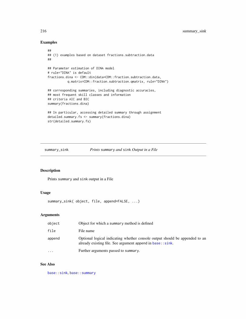
216 summary_sink

Examples


## Parameter estimation of DINA model# rule="DINA" is defaultfractions.dina <- CDM::din(data=CDM::fraction.subtraction.data,

q.matrix=CDM::fraction.subtraction.qmatrix, rule="DINA")

## corresponding summaries, including diagnostic accuracies,## most frequent skill classes and information## criteria AIC and BICsummary(fractions.dina)

## In particular, accessing detailed summary through assignmentdetailed.summary.fs <- summary(fractions.dina)str(detailed.summary.fs)

summary_sink Prints summary and sink Output in a File

Description

Prints summary and sink output in a File

Usage

summary_sink( object, file, append=FALSE, ...)

Arguments

object Object for which a summary method is defined

file File name

append Optional logical indicating whether console output should be appended to analready existing file. See argument append in base::sink.

... Further arguments passed to summary.

See Also

base::sink, base::summary

vcov 217

Examples

############################################################################## EXAMPLE 1: summary_sink example for lm function#############################################################################

#--- simulate some dataset.seed(997)N <- 200x <- stats::rnorm( N )y <- .4 * x + stats::rnorm(N, sd=.5 )

#--- fit a linear model and sink summary into a filemod1 <- stats::lm( y ~ x )

CDM::summary_sink(mod1, file="my_model")

#--- fit a second model and append it to filemod2 <- stats::lm( y ~ x + I(x^2) )CDM::summary_sink(mod2, file="my_model", append=TRUE )

vcov Asymptotic Covariance Matrix, Standard Errors and Confidence In-tervals

Description

Computes the asymptotic covariance matrix for din objects. The covariance matrix is computedusing the empirical cross-product approach (see Paek & Cai, 2014).

In addition, an S3 method IRT.se is defined which produces an extended output including vcovand confint.

Usage

## S3 method for class 'din'vcov(object, extended=FALSE, infomat=FALSE,ind.item.skillprobs=TRUE,

ind.item=FALSE, diagcov=FALSE, h=.001,...)

## S3 method for class 'din'confint(object, parm, level=.95, extended=FALSE,

ind.item.skillprobs=TRUE, ind.item=FALSE, diagcov=FALSE, h=.001, ... )

IRT.se(object, ...)

## S3 method for class 'din'IRT.se( object, extended=FALSE, parm=NULL, level=.95,

infomat=FALSE, ind.item.skillprobs=TRUE, ind.item=FALSE,diagcov=FALSE, h=.001, ... )

218 vcov

Arguments

object An object inheriting from class din.

extended An optional logical indicating whether the covariance matrix should be calcu-lated for an extended set of parameters (estimated and derived parameters).

infomat An optional logical indicating whether the information matrix instead of thecovariance matrix should be the output.

ind.item.skillprobs

Optional logical indicating whether the covariance between item parameters andskill class probabilities are assumed to be zero.

ind.item Optional logical indicating whether covariances of item parameters between dif-ferent items are zero.

diagcov Optional logical indicating whether all covariances between estimated parame-ters are set to zero.

h Parameter used for numerical differentiation for computing the derivative of thelog-likelihood function.

parm Vector of parameters. If it is missing, then for all estimated parameters a confi-dence interval is calculated.

level Confidence level

... Additional arguments to be passed.

Value

coef: A vector of parameters.

vcov: A covariance matrix. The corresponding coefficients can be extracted as the attribute coeffrom this object.

IRT.se: A data frame containing coefficients, standard errors and confidence intervals for all pa-rameters.

References

Paek, I., & Cai, L. (2014). A comparison of item parameter standard error estimation proceduresfor unidimensional and multidimensional item response theory modeling. Educational and Psycho-logical Measurement, 74(1), 58-76.

See Also

din, coef.din

Examples

## Not run:############################################################################## EXAMPLE 1: DINA model sim.dina#############################################################################

data(sim.dina, package="CDM")

vcov 219

data(sim.qmatrix, package="CDM")


#****** Model 1: DINA Modelmod1 <- CDM::din( dat, q.matrix=q.matrix, rule="DINA")# look into parameter table of the modelmod1$partable# covariance matrixcovmat1 <- vcov(mod1 )# extract coefficientscoef(mod1)# extract standard errorssqrt( diag( covmat1))# compute confidence intervalsconfint( mod1, level=.90 )# output table with standard errorsIRT.se( mod1, extended=TRUE )

#****** Model 2: Constrained DINA Model

# fix some slipping parametersconstraint.slip <- cbind( c(2,3,5), c(.15,.20,.25) )# set some skill class probabilities to zerozeroprob.skillclasses <- c(2,4)# estimate modelmod2 <- CDM::din( dat, q.matrix=q.matrix, guess.equal=TRUE,

constraint.slip=constraint.slip, zeroprob.skillclasses=zeroprob.skillclasses)# parameter tablemod2$partable# freely estimated coefficientscoef(mod2)# covariance matrix (estimated parameters)vmod2a <- vcov(mod2)sqrt( diag( vmod2a)) # standard errorscolnames( vmod2a )names( attr( vmod2a, "coef") ) # extract coefficients

# covariance matrix (more parameters, extended=TRUE)vmod2b <- vcov(mod2, extended=TRUE)sqrt( diag( vmod2b))attr( vmod2b, "coef")# attach standard errors to parameter tablepartable2 <- mod2$partablepartable2 <- partable2[ ! duplicated( partable2$parnames ), ]partable2 <- data.frame( partable2, "se"=sqrt( diag( vmod2b)) )partable2

# confidence interval for parameter "skill1" which is not in the model# cannot be calculated!confint(mod2, parm=c( "skill1", "all_guess" ) )# confidence interval for only some parameters

220 WaldTest

confint(mod2, parm=paste0("prob_skill", 1:3 ) )

# compute only information matrixinfomod2 <- vcov(mod2, infomat=TRUE)

## End(Not run)

WaldTest Wald Test for a Linear Hypothesis

Description

Computes a Wald Test for a parameter θ with respect to a linear hypothesisRθ = c.

Usage

WaldTest( delta, vcov, R, nobs, cvec=NULL, eps=1E-10 )

Arguments

delta Estimated parameter

vcov Estimated covariance matrix

R Hypothesis matrix

nobs Number of observations

cvec Hypothesis vector

eps Numerical value is added as ridge parameter of the covariance matrix

Value

A vector containing the χ2 statistic (X2), degrees of freedom (df), p value (p) and RMSEA statistic(RMSEA).

Index

∗Topic packageCDM-package, 4

abs_approx (CDM-utilities), 10abs_approx_D1 (CDM-utilities), 10anova, 6, 18anova.din, 67, 126, 128, 137anova.gdina, 100anova.gdm, 119

base::sink, 172, 216base::summary, 216

car::deltaMethod, 62cat_paste (CDM-utilities), 10cdi.kli, 8, 18, 83, 84CDM (CDM-package), 4CDM-package, 4CDM-utilities, 10cdm.est.class.accuracy, 14, 18, 84cdm_attach_internal_function

(CDM-utilities), 10cdm_calc_information_criteria

(CDM-utilities), 10cdm_fa1 (CDM-utilities), 10cdm_fit_normal (CDM-utilities), 10cdm_matrix1 (CDM-utilities), 10cdm_matrix2 (CDM-utilities), 10cdm_matrixstring (CDM-utilities), 10cdm_parameter_regularization

(CDM-utilities), 10cdm_pem_acceleration (CDM-utilities), 10cdm_pem_acceleration_assign_output_parameters

(CDM-utilities), 10cdm_pem_inits (CDM-utilities), 10cdm_pem_inits_assign_parmlist

(CDM-utilities), 10cdm_penalty_threshold_elnet

(CDM-utilities), 10

cdm_penalty_threshold_lasso(CDM-utilities), 10

cdm_penalty_threshold_mcp(CDM-utilities), 10

cdm_penalty_threshold_ridge(CDM-utilities), 10

cdm_penalty_threshold_scad(CDM-utilities), 10

cdm_penalty_threshold_scadL2(CDM-utilities), 10

cdm_penalty_threshold_tlp(CDM-utilities), 10

cdm_penalty_values (CDM-utilities), 10cdm_print_summary_call (CDM-utilities),

10cdm_print_summary_computation_time

(CDM-utilities), 10cdm_print_summary_data_frame

(CDM-utilities), 10cdm_print_summary_information_criteria

(CDM-utilities), 10CDM_rbind_fill (CDM-utilities), 10CDM_require_namespace (CDM-utilities),

10CDM_rmvnorm (CDM-utilities), 10coef, 16coef.din, 218coef.IRT.jackknife (IRT.jackknife), 142confint.din (vcov), 217csink (osink), 172

Data-sim, 17data.cdm, 18data.cdm01 (data.cdm), 18data.cdm02 (data.cdm), 18data.cdm03 (data.cdm), 18data.cdm04 (data.cdm), 18data.cdm05 (data.cdm), 18data.cdm06 (data.cdm), 18data.cdm07 (data.cdm), 18

221

222 INDEX

data.cdm08 (data.cdm), 18data.cdm09 (data.cdm), 18data.cdm10 (data.cdm), 18data.dcm, 24data.dtmr, 29data.ecpe, 31data.fraction, 34data.fraction1 (data.fraction), 34data.fraction2 (data.fraction), 34data.fraction3 (data.fraction), 34data.fraction4 (data.fraction), 34data.fraction5 (data.fraction), 34data.hr, 38data.jang, 41data.melab, 43data.mg, 46data.pgdina, 47data.pisa00R, 48data.sda6, 50data.Students, 52data.timss03.G8.su, 53data.timss07.G4.lee, 55data.timss07.G4.py

(data.timss07.G4.lee), 55data.timss07.G4.Qdomains

(data.timss07.G4.lee), 55data.timss11.G4.AUT, 58data.timss11.G4.sa

(data.timss11.G4.AUT), 58deltaMethod, 61din, 7, 8, 16, 18, 63, 65, 67, 74–76, 78, 82, 84,

86, 99, 100, 119, 131, 132, 134–136,138, 141, 145, 146, 148, 155, 161,164, 166, 175, 176, 178, 181, 187,197, 198, 214, 215, 218

din.deterministic, 74din.equivalent.class, 76, 81din.validate.qmatrix, 77din_identifiability, 80discrim.index, 9, 67, 81, 101

entropy.lca, 84equivalent.dina, 85eval_likelihood, 87

fraction.subtraction.data, 5, 37, 89fraction.subtraction.qmatrix, 5, 89, 90,

90

gdd, 91gdina, 7, 8, 16, 18, 67, 82, 84, 92, 96, 110,

113, 119, 131, 132, 134–136, 138,141, 145, 146, 148, 155, 161, 164,166, 178, 181–184, 190, 191, 196,197, 202

gdina.dif, 101, 110gdina.wald, 100, 112GDINA::att.structure, 198GDINA::dif, 111GDINA::ecpe, 32GDINA::extract, 83GDINA::frac20, 38GDINA::GDINA, 101GDINA::indlogLik, 145GDINA::indlogPost, 145GDINA::modelcomp, 113GDINA::Qval, 78GDINA::simGDINA, 191gdm, 7, 16, 114, 131, 132, 134–136, 138, 141,

145, 148, 155, 161, 166

ideal.response.pattern, 125IRT.anova, 7, 126IRT.classify, 126IRT.compareModels, 126, 127, 137IRT.data, 130, 135, 194IRT.derivedParameters (IRT.jackknife),

142IRT.expectedCounts, 132IRT.factor.scores, 127, 133IRT.frequencies, 135IRT.IC, 128, 136IRT.irfprob, 88, 135, 137, 139, 179IRT.irfprobPlot, 137, 138, 139, 178IRT.itemfit, 140IRT.jackknife, 142, 151IRT.likelihood, 127, 134, 138, 141, 144, 148IRT.marginal_posterior, 146IRT.modelfit, 127, 128, 147IRT.parameterTable, 149IRT.posterior, 127, 134, 135, 138, 141, 146,

148, 179, 194IRT.posterior (IRT.likelihood), 144IRT.predict (predict), 178IRT.repDesign, 142, 150IRT.RMSD, 151, 154IRT.se (vcov), 217

INDEX 223

IRT_frequencies_default(IRT.frequencies), 135

IRT_frequencies_wrapper(IRT.frequencies), 135

IRT_RMSD_calc_rmsd (IRT.RMSD), 151item_by_group, 159itemfit.rmsea, 65, 98, 118, 141, 151, 153,

154itemfit.sx2, 18, 67, 100, 119, 155

logLik, 126, 127, 136, 137, 160

mcdina, 7, 16, 18, 84, 131, 132, 134, 135, 138,145, 146, 161, 161

mirt::numerical_deriv, 171modelfit.cor, 165modelfit.cor.din, 18, 67, 100, 119, 147, 148modelfit.cor2 (modelfit.cor), 165

numerical_gradient (numerical_Hessian),170

numerical_Hessian, 170numerical_Hessian_partial

(numerical_Hessian), 170

osink, 172

personfit.appropriateness, 173plot.din, 5, 65, 67, 175, 181, 187, 215plot.gdina (gdina), 92plot.gdm (gdm), 114plot.itemfit.sx2 (itemfit.sx2), 155plot.personfit.appropriateness

(personfit.appropriateness),173

plot.slca (slca), 200plot_item_mastery, 177predict, 178predict.din (predict), 178predict.gdina (predict), 178predict.gdm (predict), 178predict.mcdina (predict), 178predict.slca (predict), 178prep_data_long_format

(eval_likelihood), 87print.din, 5, 65, 67, 176, 181, 215print.din (din), 63print.gdina (gdina), 92print.gdm (gdm), 114

print.mcdina (mcdina), 161print.slca (slca), 200print.summary.din, 5, 176, 180, 187, 215

reglca, 131, 138, 141, 145, 161, 181

sequential.items, 184sim.din, 5, 186, 190sim.dina (Data-sim), 17sim.dino (Data-sim), 17sim.gdina, 100, 190sim.qmatrix (Data-sim), 17sim_model, 187, 191, 193sirt::rasch.mml, 155sirt::smirt, 155skill.cor, 195skill.polychor (skill.cor), 195skillspace.approximation, 196skillspace.full (skillspace.hierarchy),

197skillspace.hierarchy, 197slca, 7, 16, 131, 132, 134, 135, 138, 141, 145,

161, 183, 200stats::p.adjust, 156, 166summary, 180summary.cdi.kli (cdi.kli), 8summary.din, 5, 65, 67, 176, 180, 181, 187,

214, 215summary.din_identifiability

(din_identifiability), 80summary.discrim.index (discrim.index),

81summary.entropy.lca (entropy.lca), 84summary.gdina (gdina), 92summary.gdina.dif (gdina.dif), 110summary.gdina.wald (gdina.wald), 112summary.gdm (gdm), 114summary.IRT.compareModels

(IRT.compareModels), 127summary.IRT.modelfit.din

(IRT.modelfit), 147summary.IRT.modelfit.gdina

(IRT.modelfit), 147summary.IRT.RMSD (IRT.RMSD), 151summary.itemfit.sx2 (itemfit.sx2), 155summary.mcdina (mcdina), 161summary.modelfit.cor.din

(modelfit.cor), 165

224 INDEX

summary.personfit.appropriateness(personfit.appropriateness),173

summary.reglca (reglca), 181summary.slca (slca), 200summary_sink, 216

TAM::tam.mml, 155TAM::tam.modelfit.IRT, 148

vcov, 217vcov.din (vcov), 217vcov.IRT.jackknife (IRT.jackknife), 142

WaldTest, 220

Package ‘CDM’ - R · The package CDM is implemented based on the S3 system. It comes with a...

Documents

Transcript of Package ‘CDM’ - R · The package CDM is implemented based on the S3 system. It comes with a...