P-y Curve (Korean Paper)

8/11/2019 P-y Curve (Korean Paper)

http://slidepdf.com/reader/full/p-y-curve-korean-paper 1/16

Yang et al. 1

Dynamic p-y Backbone Curves from 1g Shaking Table Tests

Eui Kyu Yang

Ph. D. Student, Department of Civil Engineering, Seoul National University, San 56-1, Shinlim-Dong, Kwanak-Ku, Seoul, 151-742, Korea, Tel: (82)-2-880-8732, Fax (82)-2-875-6933, E-mail:[email protected]

Sang Seom Jeong

Professor, Department of Civil & Environmental Engineering, College of Engineering, YonseiUniversity, Seoul, 120-749, Korea, Tel: (82)-2-2123-2807, Fax (82)-2-364-5300, E-mail:[email protected]

Jeong Hwan Kim

Deputy General Manager/Ph.D, Department of Overseas Civil Eng Project, Civil Division,Samsung C&T Corporation, Seoul, 137-857, Korea, Tel: (82)-2-2145-6024, Fax (82)-2-2145-6060, E-mail: [email protected]

Myoung Mo Kim

Professor, Department of Civil Engineering, Seoul National University, San 56-1, Shinlim-Dong,Kwanak-Ku, Seoul, 151-742, Korea, Tel: (82)-2-880-7348, Fax (82)-2-875-6933, E-mail:[email protected] (corresponding author)

Length of Manuscript

Number of words (2654) + Figure 11(2750) + Table 4(1000) = 6404 < 7500

Submission date

August 1, 2008

TRB 2009 Annual Meeting CD-ROM Paper revised from original submittal.



Yang et al. 3

INTRODUCTIONIn seismic design of a pile foundation, pseudo-static analysis is widely used to convertdynamic loads to equivalent static loads. Among the diverse methods of modeling foundationsfor pseudo-static analysis, the p-y curve method considering non linear soil behavior is most

frequently used in practice. For static loading conditions, O’Neil and Reese’s p-y curves(1,2,3) ,obtained from various full scale pile load tests, are commonly used, and they are appliedeven for seismic loading conditions with slight modifications without strict verification due tothe lack of well-established dynamic p-y curves for seismic conditions. Research has shown thatp-y curves for static loading conditions are not applicable to dynamic loading conditions (4, 5) .Various p-y curves applied in pseudo-static analysis for seismic design are summarized inTABLE 1.

TABLE 1 Existing P-y Curve Methods

Reference Equation of p-y curves Remarks

API (1) ,O’Neill (2)

tanh( )uu

kz p Ap y

Ap=

where u p = minimum value of 1 2( )C z C D zγ + and 3C D zγ ;

1 2 3, ,C C C = constants; A = constants according to loading type

Developed from backanalysis of full scale

instrumented static andcyclic pile load tests on

sand

Reese (3)

a h a

z p k y

D= and b u

B p p

A=

u p = minimum value between us p and ud p ;

, A B = empirical factors; a y = / 1 1/ 1( / ) ( / )n m mb h b D p zk D y− −

;

b y = / 60 D ; u y = 3 /80 D

Developed from theresults of full scale

static and cyclicloading tests

NCHRP (6)

20 0 ,

n

d s d u

y p p a p p

d

α βα κ

= + + ≤

where s p = static soil reaction; , , , nα β κ = constants;

= frequency of loading; 0a = dimensionless frequency

The equation wasestablished from

computational model.

JRA (7)

Modulus of subgrade reaction HE k k H k n a k =

ultimate soil resistance HU p p u p n a p=

where , , ,k k p pn a n a = constants

N/A

Note) N/A: Not available

In this study a series of 1g shaking table tests were carried out for various conditions ofacceleration frequency, acceleration amplitude for input load, flexural stiffness of a pile shaft andmass at the pile head. P-y curves for each test conditions were evaluated and dynamic p-ybackbone curves for pseudo static analysis were obtained, and compared with p-y curves used inpractice. The applicability of the dynamic p-y backbone curves suggested in this study wasevaluated based on the test results of other researchers cited in literature.




Yang et al. 4

DESCRIPTION OF EXPERIMENTAL TESTING PROGRAMA biaxial shaking table was used to perform a dynamic model pile test under 1g condition. Thebiaxial table of 2000mm width and 2000 mm length had a maximum capacity of sample weight,acceleration and frequency of 5 tons, 1 g and 50Hz, respectively.

A soil box made of transparent acrylic plates of 1800 mm length, 600 mm width, and

1200 mm height was placed on the shaking table. Sponges of 50 mm thickness were attachedinside the short side walls of the soil box to reduce the reflection waves developed by the rigidwall in the shaking direction.

A model pile with a hollow circular section was made of aluminum alloy. The propertiesof the model pile and pile cap, including the embedded depth and flexural rigidity, are listed inTABLE 2. The thickness of the hollow cylindrical pile and the mass at the pile head were variedfor each test for parametric study.

TABLE 2 Properties of Model Piles

Properties ValuesMaterial Aluminum alloy pipeEmbedded depth (cm) 110Outer diameter (cm) 3.2Thickness (cm) 0.5, 0.3, 0.2Elastic modulus (Gpa) 67.82Flexural rigidity (kgf-cm 2) 2764424 (EI), 2008342 (0.72EI),1473056 (0.53EI)Mass (kg) 0, 64, 96, 192

Jumoonjin sand, characterized as clean and uniform sand, was used in these tests. The

properties of Jumoonjin sand are listed in TABLE 3. The sand layer was prepared by pouring drysand into the soil box in 5 steps, and then, in each step, the poured sand was compacted carefullyby shaking the table with 0.4g sine wave vibration at 10 Hz to obtain the relative density of 80%.

TABLE 3 Properties of Jumoonjin Sand

USCS D 10 (mm) D50 (mm) C u G s

γ d,max (t/m 3)

γ d,min (t/m 3)

SP 0.38 0.58 1.68 2.65 1.66 1.33

FIGURE 1 shows the test set-up with the schematic of the layout for instrumentation. A

model pile was fixed to the bottom of the soil box to reproduce an actual pile in weathered rock.The pile was positioned first and then soil was poured to make the soil-pile system. The pile capwas located 11cm above the subsurface, and its mass was changed to generate different inertialforces. The pile was instrumented by bonding miniature strain gauges in pairs at seven locationsalong the pile to measure the bending moment. At the same depths as the gauges, accelerometerswere set up to monitor the free field displacement of the soil. LVDT and another accelerometerwere set up at the pile cap to monitor the displacement and inertial force of the superstructure.An input sine wave of 0.09g ~ 0.4g amplitude and 3Hz ~ 15Hz frequency was applied at the baseof the soil box for about 4 seconds.




Yang et al. 5

4

16

unit : cm

8

12

20

24

26

11

AccelerometerStrain GaugeLVDT

Shaking of Soil Container : Sine Wave

32

4

16

unit : cm

8

12

20

24

26

11

AccelerometerStrain GaugeLVDT

Shaking of Soil Container : Sine Wave

32

(a) Test box with full instrumentations (b) Schematic drawing for instrumentation

FIGURE 1 Test set-up

Test programs are summarized in TABLE 4.

TABLE 4 Test Programs

Testnumber

Loadingfrequency (Hz)

Loadingamplitude (g)

Pilestiffness (ratio)

Surchargeload (kg)

Case 1 6, 12 0.09, 0.154, 0.3, 0.4 1 96Case 2 6 0.154, 0.4 1 0, 64, 96, 192Case 3 3,6,9,12,15 0.154, 0.4 1 96Case 4 6 0.154, 0.4 1, 0.72, 0.53 96

DETERMINATION OF EXPERIMENTAL DYNAMIC P-Y CURVESP-y curves are derived from bending moments measured along a pile based on the simple beamtheory (8) . Lateral soil resistance ( p ) and pile displacement ( pile y ) are obtained by double

differentiation and double integration of bending moments, respectively:2

2 ( )d

p M zdz

= (1)

( ) pile

M z y dz

EI = ∫∫ (2)

where, p is the lateral resistance of soil; pile y is the lateral displacement of the pile; ( ) M z are

the measured bending moments along the pile; EI is the flexural rigidity of the pile; z is thedepth below ground surface.

The experimental bending moments are only calculated at certain discrete locations alongthe pile so a curve-fitting technique is necessary to obtain the soil resistance and displacementalong the pile length continuously. The cubic spline method was used as the curve-fitting




Yang et al. 6

technique. To remove noise data in calculating the time history of p-y values, band pass filteringwas performed by Fast Fourier Transform (FFT) analysis.

To obtain the relative displacement ( y ) for the dynamic p-y curve, the soil movement( soil y ), obtained from the free field accelerometers, was subtracted from the pile displacement

( pile

y ) at each time step. FIGURE 2 shows the horizontal displacements of the pile and soil at the

loading amplitude of 0.4g for the loading frequency of 6Hz.

0

20

40

60

80

100

120

-0.30 -0.20 -0.10 0.00 0.10 0.20 0.30

Displacement (cm)

Depth (cm)

PileSoil

FIGURE 2 Displacement distributions of soil and pile (0.4g, 6Hz)

TEST RESULTS

Experimental P-y CurveAs mentioned, a series of 1g shaking table tests were performed for different flexural rigidities ofthe piles and for various masses at various amplitudes and frequencies of input accelerations. As

the test results, experimental p-y curves were obtained. FIGURES 3(a), (b), (c) and (d) showsome experimental curves. For case (a) of the figure, it is noticed that the experimental curvesare influenced little by the change of the flexural rigidity of the pile. When the pile head load isvaried (case (b)), the slope of the p-y curves maintains almost constant, but the dynamic soilreactive force increases as the head load decreases, which may be attributed to the fact that pilehead movement increases at a steeper rate than the decrease rate of the pile head load. Fordifferent amplitudes of the input acceleration (case (c)), the reactive soil force changes little, butthe slope of the curve decreases as the amplitude increases. When the frequency of the inputacceleration is varied (case (d)), the shape of experimental curve changes abruptly at a certainfrequency, which may be interrelated with the magnitude of the natural frequency of the pile soilsystem and that of the input frequency.




Yang et al. 7

p-y (3.75D)

-30

-20

-10

0

10

20

30

-0.30 -0.20 -0.10 0.00 0.10 0.20 0.30

y(cm)

p(N/cm)

0.53EI

0.72EI

EI

p-y (3.75D)

-30

-20

-10

0

10

20

30

-0.30 -0.20 -0.10 0.00 0.10 0.20 0.30

y(cm)

p(N/cm)

0.53EI

0.72EI

EI

p-y (3.75D)

-40

-30

-20

-10

0

10

20

30

40

-0.30 -0.20 -0.10 0.00 0.10 0.20 0.30

y(cm)

p(N/cm)

192kg

96kg64kg

p-y (3.75D)

-40

-30

-20

-10

0

10

20

30

40

-0.30 -0.20 -0.10 0.00 0.10 0.20 0.30

y(cm)

p(N/cm)

192kg

96kg64kg

(a) For different flexural rigidities of piles, EI (b) For different masses of pile head(0.4g, 6Hz, 96kg) (0.4g, 6Hz)

p-y (3.75D)

-30

-20

-10

0

10

20

30

-0.30 -0.20 -0.10 0.00 0.10 0.20 0.30

y(cm)

p(N/cm)

0.4g0.3g

0.154g

0.09g

p-y (3.75D)

-30

-20

-10

0

10

20

30

-0.30 -0.20 -0.10 0.00 0.10 0.20 0.30

y(cm)

p(N/cm)

0.4g0.3g

0.154g

0.09g

p-y (3.75D)

-30

-20

-10

0

10

20

30

-0.30 -0.20 -0.10 0.00 0.10 0.20 0.30

y(cm)

p(N/cm)

6Hz, 0.4g

9Hz, 0.4g

6Hz, 0.154g

12Hz, 0.4g

15Hz, 0.4g

p-y (3.75D)

-30

-20

-10

0

10

20

30

-0.30 -0.20 -0.10 0.00 0.10 0.20 0.30

y(cm)

p(N/cm)

6Hz, 0.4g

9Hz, 0.4g

6Hz, 0.154g

12Hz, 0.4g

15Hz, 0.4g

(c) For different amplitudes of input acceleration (d) For different frequencies of input

acceleration (6Hz, 96kg) (0.4g, 6Hz)

FIGURE 3 Experimental dynamic p-y curves

DEFINITION OF DYNAMIC P-Y BACKBONE CURVEBased on the experimental p-y curve data, the dynamic p-y backbone curves, which are used forpseudo-static analysis of dynamically loaded pile systems, can be constructed. First, the peakpoints of the experimental p-y curves, which correspond to the maximum soil resistance, weretaken at several points (coincide with the locations of the strain gages), and plotted on a p-yplane for each location as shown in FIGURE 4. And then, a best-fit curve was pursued for eachdepth by regression analysis. The basic equation of the best-fit curve was chosen to be thehyperbolic function of Kondner (9), ,

1

ini u

y p

yk p

=

+

(3)

where, inik is the initial subgrade modulus; u p is the ultimate soil resistance; y is thehorizontal deflection of the pile.




Yang et al. 8

0

2

4

6

8

10

12

14

0.00 0.10 0.20 0.30 0.40 0.50

y(cm)

p(N/c m)

3Hz 6Hz 12Hz Low er li mit Upp er li mit

0

5

10

15

20

25

30

35

40

45

50

0.00 0.10 0.20 0.30 0.40 0.50

y(cm)

p(N/cm)

3Hz 6Hz 12Hz Low er li mit Uppe r li mit

(a) At the depth of 1.25 diameters (b) At the depth of 3.75 diameters

FIGURE 4 Lower limit and Upper limit p-y Backbone curves

PROPOSED DYNAMIC P-Y BACKBONE CURVESAs are seen in FIGURES 4(a) and 4(b), the points plotted on the p-y planes are widely scattered.Thus to embrace all the data points, two limit backbone curves were established for each depth,i.e., upper limit and lower limit curves. To express these curves as a hyperbolic function, theinitial slope of the curve ( inik ) and the asymptotic value of the soil reaction ( u p ) should beexpressed as an equation.

Determination of Ultimate Soil Resistance ( u p )FIGURE 5(a) shows the lower limit p-y backbone curves at several depths. The ultimate soilresistance was best-fitted using Equation 4 (10).

' nu p

p AK z D γ = (4)

where, pK is the Rankine’s passive pressure coefficient; 'γ is the effective unit weight; D is

the pile diameter; and , A n are curve-fitting constants. Through regression analysis (FIGURE5(b)), , A n were found to be 6.32 and 1.22 for the lower limit backbone curve, and 11.83 and1.11 for the upper limit backbone curve, respectively. Thus, u p can be obtained by thefollowing equations.

Lower Limit p-y Backbone curve: ' 1.226.32u p

pK z

Dγ = ( 2 / N cm ) (5)

Upper Limit p-y Backbone curve:' 1.11

11.83u

p

pK z D γ

= (

2

/ N cm ) (6)




Yang et al. 11

3 .7 5D

0

5

1 0

1 5

2 0

2 5

3 0

3 5

4 0

4 5

0 .0 0 0 .1 0 0 .2 0 0 .3 0 0 .4 0 0 .5 0

y( cm )

p (N /c m )

3 Hz 6 Hz 1 2 Hz Su gg es t(M i n) Su gg es t( M ax )

Ja pa n A PI C yc lic , N C H R P 6H z

Upper l imit

Lo w er lim it

3 .7 5D

0

5

1 0

1 5

2 0

2 5

3 0

3 5

4 0

4 5

0 .0 0 0 .1 0 0 .2 0 0 .3 0 0 .4 0 0 .5 0

y( cm )

p (N /c m )



3 .7 5D

0

5

1 0

1 5

2 0

2 5

3 0

3 5

4 0

4 5

0 .0 0 0 .1 0 0 .2 0 0 .3 0 0 .4 0 0 .5 0

y( cm )

p (N /c m )



Upper l imit

Lo w er lim it

(b) At the depth of 3.75 diameters

7 . 5D

0

1 0

2 0

3 0

4 0

5 0

6 0

7 0

8 0

0 .0 0 0 .1 0 0 .2 0 0 .3 0 0 .4 0 0 .5 0

y( cm )

p (N/c m )

3 Hz 6 Hz Su g g es t( M in ) Su g ge st (M a x )

Ja pa n

AP I C yc lic , N C H RP 6H zUpper l imit

L ow er lim it

7 . 5D

0

1 0

2 0

3 0

4 0

5 0

6 0

7 0

8 0

0 .0 0 0 .1 0 0 .2 0 0 .3 0 0 .4 0 0 .5 0

y( cm )

p (N/c m )

3 Hz 6 Hz Su g g es t( M in ) Su g ge st (M a x )

Ja pa n

AP I C yc lic , N C H RP 6H zUpper l imit

L ow er lim it

(c) At the depth of 7.5 diameters

FIGURE 7 Comparison of p-y curves

In FIGURE 8, measured bending moments and lateral deflections of piles are comparedwith the predicted values obtained from various methods. For the bending moments, all theexisting methods overpredict by up to 50%. For the lateral deflection, upper limit backbonecurve predicts most closely to the measured values.




Yang et al. 12

Measur ed an d Cal cula ted B ending M oment

0

20

40

60

80

100

120

-1000 0 1000 2000 3000 4000 5000 6000 7000

Moment (Ncm)

D e p t h ( c m

) Upper Limit

Meas ured

Lowe r Lim it

NCHR P

Japa n

API C yclic

Measur ed an d Cal cula ted B ending M oment

0

20

40

60

80

100

120

-1000 0 1000 2000 3000 4000 5000 6000 7000

Moment (Ncm)

D e p t h ( c m

) Upper Limit

Meas ured

Lowe r Lim it

NCHR P

Japa n

API C yclic

(a) Bending moment profiles

Measured and Calculat ed Displ acement

0

20

40

60

80

100

120

-0.05 0 0.05 0.1 0.15 0.2

Displ acement(cm)

D e p t h

( c m )

Upper Limit

Measured

Lower Limit Japan, NCHRP

API Cyclic

Measured and Calculat ed Displ acement

0

20

40

60

80

100

120

-0.05 0 0.05 0.1 0.15 0.2

Displ acement(cm)

D e p t h

( c m )

Upper Limit

Measured

Lower Limit Japan, NCHRP

API Cyclic

(b) Lateral deflections

FIGURE 8 Measured and predicted results based on pseudo-static analysis

APPLICABILITY OF SUGGESTED DYNAMIC P-Y BACKBONE CURVES

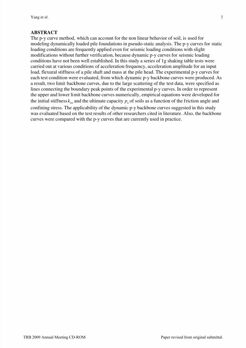
The applicability of dynamic p-y backbone curves suggested in this study was evaluated basedon the test results obtained by various researchers (5, 12, 13) . FIGURE 9 shows the results of thedynamic pile load tests performed by Chenaf et al. (12) using an electromagnetic gun onFontainebleau dry sand. The thick lines of FIGURES 9(a), (b) and (c) represent the experimentaldynamic p-y curves at different depths. The upper limit p-y backbone curve and the lower limitp-y backbone curve are represented in the same figure for direct comparison. It is clear that thepeak points of the dynamic p-y curves at depths of 0.6m and 1.2m are located in between theupper and lower limit p-y backbone curves, while the peak points of the dynamic p-y curve at adepth of 1.8m lie on the upper limit p-y backbone curve. Therefore, it is concluded that thesuggested p-y backbone curves compare well with the test results.




Yang et al. 14

(a) At the depth of 1 diameter (b) At the depth of 2 diameters

(c) At the depth of 3 diameters (d) At the depth of 4 diameters

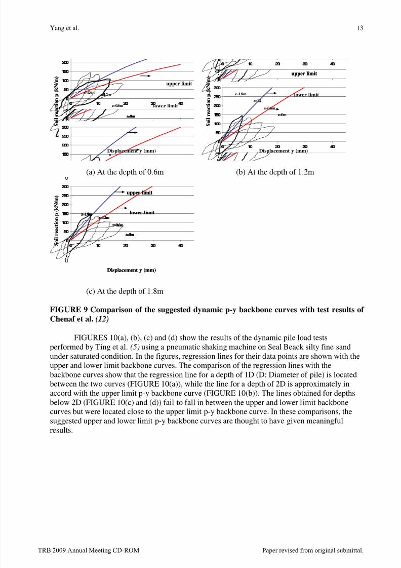
FIGURE 10 Comparison of the suggested dynamic p-y backbone curves with test results ofTing et al. (5)

Pseudo-static analysis was conducted using the p-y backbone curves to predict the resultsof the dynamic pile load tests performed in the centrifuge. FIGURE 11 shows the bendingmoment curve obtained from the centrifuge (13) together with the curves obtained by thepseudo-static analysis. The comparison of the three curves indicates that the pseudo-staticanalysis provides a good estimate of the bending moment against depth.




Yang et al. 15

Measured and Calculated Bending Moment

0

5

10

15

20

25

30

35

-1000 0 1000 2000 3000 4000 5000 6000

Moment(kNm)

D e p t h

( m )

Experiment

Lower Limit Upper Limit

Measured and Calculated Bending Moment

0

5

10

15

20

25

30

35

-1000 0 1000 2000 3000 4000 5000 6000

Moment(kNm)

D e p t h

( m )

Experiment

Lower Limit Upper Limit

FIGURE 11 Comparison of test results of Kotthaus et al. (13) with pseudo-static analysis

CONCLUSIONSA series of 1g shaking table tests were performed to obtain dynamic p-y curves for use inpseudo-static analysis of earthquake-loaded pile foundations. Based on the test results, thefollowing conclusions are drawn.

1. Dynamic p-y backbone curves were produced as two limit lines (upper and lower limits)connecting the boundary peak points of experimental p-y curves.

2. To represent the backbone curves numerically, empirical equations were developed forthe initial stiffness ( inik ) and the ultimate capacity of soil ( u p ) as a function of thefriction angle of the soil and the confining stress.

3. The existing p-y curves used for dynamically loaded piles predicted soil resistances thatwere much smaller than the measured values (smaller than one half of the measuredones) at shallow depths of the piles. The lateral behavior of piles at shallow depths is ofutmost importance.

4. The applicability of the proposed dynamic backbone curves was confirmed based on thecomparisons with the test results of various researchers.

ACKNOWLEDGMENTSThis research is supported by National Research Laboratory Program (ROA-2007-000-1004-0),which is supervised by Ministry of Education Science and Technology, MEST.

REFERENCE1. American Petroleum Institute. Recommended practice for planning, designing andconstructing fixed offshore platforms. API Recommended Practice 2A (RP-2A) , 17 th edition.,1987.

2. O’Neill. M. W., and Murchinson, J.M. An evaluation of p-y relationships in sand. Rep.Prepared for American Petroleum Institute ,Washington,D.C.,1983.

3. Reese, L.C., Cox, W.R. and Koop, F.D. Analysis of laterally loaded piles in sand.Proceedings of the VI Annual Offshore Technology Conference , Houston, 1974, pp.473-485.




Yang et al. 16

4. Dou, H., and Byrne, P.M. Dynamic response of single piles and soil-pile interaction.Canadian Geotechnical Journal , 1996, Vol.33, pp.80-96.

5. Ting, J.M., Kauffman, C.R., Lovicsek, M. Centrifuge static and dynamic lateral pilebehaviour. Canadian Geotechnical Journal , 1987, Vol.24, pp.198-207.

6. National Cooperative Highway Research Program. Static and dynamic lateral loading of pile

groups. NCHRPReport461 , Transportation Research Board-National Research Council, 2001.7. Japan Road Association (JRA). Specification for highway bridges , 2002.8. Hetenyi, M.. Beams on elastic foundation , University of Michigan Press Ann Arbor, MI,

19469. Kondner, R.L. Hyperbolic stress-strain response: Cohesive soils. J. Soil Mechanics and

Foundation Div. , ASCE, 1963, 89(1), 115-14410. Byung Tak Kim, Nak-Kyung Kim, Woo Jin Lee, and Young Su Kim. Experimental load-

transfer curves of laterally loaded piles in Nak-Dong river sand. Journal of Geotechnical andGeoenvironmental Engineering , 2004, Vol. 130, No. 4, April 1.

11. Janbu, N. Soil compressibility as determined by oedometer and triaxial test. Proceedings ofthe European Conference on Soil Mechanics and Foundations Engineering , Wiesbaden,Germany, 1963, Vol1. pp. 19-25

12. N.Chenaf, J.L. Chazelas & L.Thorel. Comparison of dynamic and cyclic behavior of piles insand submitted to horizontal loading: Centrifuge tests. Physical Modelling in Geotechnics –6 th ICPMG’06 , Vol2, 2006, pp.979–984.

13. M.Kotthaus, T.Grundhoff & H.L.Jessberger. Single piles and pile rows subjected to staticand dynamic lateral load. Proceeding of the international conference centrifuge 94 , 1994,pp.497–502.

P-y Curve (Korean Paper)

Documents

Transcript of P-y Curve (Korean Paper)