P Values: What They Are and How to Use Them - CDF - Fermilab

Dra

ftJu

ne13

,20

07

CDF/MEMO/STATISTICS/PUBLIC/8662Version 4.00

June 13, 2007

P Values: What They Are and How to Use Them

Luc Demortier1

Laboratory of Experimental High-Energy Physics

The Rockefeller University

“Far too many scientists have only a shaky graspof the statistical techniques they are using. Theyemploy them as an amateur chef employs a cookbook, believing the recipes will work without un-derstanding why. A more cordon bleu attitude tothe maths involved might lead to fewer statisticalsouffles failing to rise.”in “Sloppy stats shame science,” The Economist,Vol. 371, No. 8378, pg. 74 (June 5th 2004).

Abstract

This note reviews the definition, calculation, and interpretation of p valueswith an eye on problems typically encountered in high energy physics. Specialemphasis is placed on the treatment of systematic uncertainties, for which severalmethods, both frequentist and Bayesian, are described and evaluated. After abrief look at some topics in the area of multiple testing, we examine significancecalculations in spectrum fits, focusing on a situation whose subtlety is often notrecognized, namely when one or more signal parameters are undefined underthe background-only hypothesis. Finally, we discuss a common search procedurein high energy physics, where the effect of testing on subsequent inference isincorrectly ignored.

[email protected]

mailto:[email protected]

Dra

ftJu

ne13

,20

07

2 CONTENTS

Contents

List of Figures 5

List of Examples 7

1 Introduction 8

2 Basic ideas underlying the use of p values 82.1 The choice of null hypothesis . . . . . . . . . . . . . . . . . . . . . . . . 112.2 The σ scale for p values and the 5σ discovery threshold . . . . . . . . . 122.3 A simple numerical example . . . . . . . . . . . . . . . . . . . . . . . . 15

2.3.1 Exact calculation . . . . . . . . . . . . . . . . . . . . . . . . . . 162.3.2 Bounds and approximations . . . . . . . . . . . . . . . . . . . . 17

3 Properties and interpretation of p values 183.1 P values versus Bayesian measures of evidence . . . . . . . . . . . . . . 193.2 P values versus frequentist error rates . . . . . . . . . . . . . . . . . . . 213.3 Dependence of p values on sample size . . . . . . . . . . . . . . . . . . 24

3.3.1 Stopping rules . . . . . . . . . . . . . . . . . . . . . . . . . . . . 243.3.2 Effect of sample size on the evidence provided by p values . . . 263.3.3 The Jeffreys-Lindley paradox . . . . . . . . . . . . . . . . . . . 273.3.4 Admissibility constraints . . . . . . . . . . . . . . . . . . . . . . 293.3.5 Practical versus statistical significance . . . . . . . . . . . . . . 29

3.4 Incoherence of p values as measures of support . . . . . . . . . . . . . . 303.4.1 The problem of regions paradox . . . . . . . . . . . . . . . . . . 303.4.2 Rao’s paradox . . . . . . . . . . . . . . . . . . . . . . . . . . . . 32

3.5 Calibration of p values . . . . . . . . . . . . . . . . . . . . . . . . . . . 323.6 P values and interval estimates . . . . . . . . . . . . . . . . . . . . . . 333.7 Alternatives to p values . . . . . . . . . . . . . . . . . . . . . . . . . . . 35

4 Incorporating systematic uncertainties 384.1 Setup for the frequentist assessment of Bayesian p values . . . . . . . . 404.2 Conditioning method . . . . . . . . . . . . . . . . . . . . . . . . . . . . 43

4.2.1 Null distribution of conditional p values . . . . . . . . . . . . . . 454.3 Supremum method . . . . . . . . . . . . . . . . . . . . . . . . . . . . . 46

4.3.1 Choice of test statistic . . . . . . . . . . . . . . . . . . . . . . . 464.3.2 Application to a likelihood ratio problem . . . . . . . . . . . . . 484.3.3 Null distribution of the likelihood ratio statistic . . . . . . . . . 504.3.4 Null distribution of supremum p values . . . . . . . . . . . . . . 514.3.5 Case where the auxiliary measurement is Poisson . . . . . . . . 53

4.4 Confidence interval method . . . . . . . . . . . . . . . . . . . . . . . . 544.4.1 Application to likelihood ratio problem . . . . . . . . . . . . . . 554.4.2 Null distribution of confidence interval p values . . . . . . . . . 57

Dra

ftJu

ne13

,20

07

CONTENTS 3

4.5 Bootstrap methods . . . . . . . . . . . . . . . . . . . . . . . . . . . . . 574.5.1 Adjusted plug-in p values; iterated bootstrap . . . . . . . . . . . 594.5.2 Case where the auxiliary measurement is Poisson . . . . . . . . 604.5.3 Conditional plug-in p values . . . . . . . . . . . . . . . . . . . . 614.5.4 Nonparametric bootstrap methods . . . . . . . . . . . . . . . . 62

4.6 Fiducial method . . . . . . . . . . . . . . . . . . . . . . . . . . . . . . . 634.6.1 Comparing the means of two exponential distributions . . . . . 654.6.2 Detecting a Poisson signal on top of a background . . . . . . . . 664.6.3 Null distribution of fiducial p values for the Poisson problem . . 69

4.7 Prior-predictive method . . . . . . . . . . . . . . . . . . . . . . . . . . 694.7.1 Null distribution of prior-predictive p values . . . . . . . . . . . 714.7.2 Robustness study . . . . . . . . . . . . . . . . . . . . . . . . . . 734.7.3 Choice of test statistic . . . . . . . . . . . . . . . . . . . . . . . 744.7.4 Asymptotic approximations . . . . . . . . . . . . . . . . . . . . 764.7.5 Subsidiary measurement with a fixed relative uncertainty . . . . 79

4.8 Posterior-predictive method . . . . . . . . . . . . . . . . . . . . . . . . 814.8.1 Posterior prediction with noninformative priors . . . . . . . . . 834.8.2 Posterior prediction with informative priors . . . . . . . . . . . 844.8.3 Choice of test variable . . . . . . . . . . . . . . . . . . . . . . . 854.8.4 Null distribution of posterior-predictive p values . . . . . . . . . 874.8.5 Further comments on prior- versus posterior-predictive p values 88

4.9 Power comparisons and bias . . . . . . . . . . . . . . . . . . . . . . . . 884.10 Summary . . . . . . . . . . . . . . . . . . . . . . . . . . . . . . . . . . 894.11 Software for calculating p values . . . . . . . . . . . . . . . . . . . . . . 90

5 Multiple testing 915.1 Combining independent p values . . . . . . . . . . . . . . . . . . . . . . 935.2 Other procedures . . . . . . . . . . . . . . . . . . . . . . . . . . . . . . 94

6 A further look at likelihood ratio tests 946.1 Testing with weighted least-squares . . . . . . . . . . . . . . . . . . . . 96

6.1.1 Exact and asymptotic pivotality . . . . . . . . . . . . . . . . . . 986.1.2 Effect of Poisson errors, using Neyman residuals . . . . . . . . . 996.1.3 Effect of Poisson errors, using Pearson residuals . . . . . . . . . 996.1.4 Effect of a non-linear null hypothesis . . . . . . . . . . . . . . . 100

6.2 Testing in the presence of nuisance parameters that are undefined underthe null . . . . . . . . . . . . . . . . . . . . . . . . . . . . . . . . . . . 1006.2.1 Lack-of-fit test . . . . . . . . . . . . . . . . . . . . . . . . . . . 1016.2.2 Finite-sample bootstrap test . . . . . . . . . . . . . . . . . . . . 1016.2.3 Asymptotic bootstrap test . . . . . . . . . . . . . . . . . . . . . 1026.2.4 Analytical upper bounds . . . . . . . . . . . . . . . . . . . . . . 1036.2.5 Other test statistics . . . . . . . . . . . . . . . . . . . . . . . . . 1046.2.6 Other methods . . . . . . . . . . . . . . . . . . . . . . . . . . . 104

Dra

ftJu

ne13

,20

07

4 CONTENTS

6.3 Summary of δX2 study . . . . . . . . . . . . . . . . . . . . . . . . . . . 1056.4 A naıve formula . . . . . . . . . . . . . . . . . . . . . . . . . . . . . . . 105

7 Effect of testing on subsequent inference 1067.1 Conditional confidence intervals . . . . . . . . . . . . . . . . . . . . . . 1087.2 Further considerations on the effect of testing . . . . . . . . . . . . . . 110

Acknowledgements 111

Appendix 112

A Laplace approximations 112

B Asymptotic distribution of the δX2 statistic 113

C Orthogonal polynomials for linear fits 118

D Fitting a non-linear model 119D.1 Asymptotic linearity and consistency . . . . . . . . . . . . . . . . . . . 120D.2 Non-linear regression with consistent estimators . . . . . . . . . . . . . 120D.3 Non-linear regression with inconsistent estimators . . . . . . . . . . . . 120

Figures 123

References 168

Dra

ftJu

ne13

,20

07

LIST OF FIGURES 5

List of Figures

1 Null distribution of conditional p values (1) . . . . . . . . . . . . . . . . 1232 Null distribution of conditional p values (2) . . . . . . . . . . . . . . . . 1243 Null distribution of conditional p values (3) . . . . . . . . . . . . . . . . 1254 Likelihood ratio tail probability versus ν . . . . . . . . . . . . . . . . . 1265 Likelihood ratio survivor function . . . . . . . . . . . . . . . . . . . . . 1276 Null distribution of likelihood ratio p values (1) . . . . . . . . . . . . . 1287 Null distribution of likelihood ratio p values (2) . . . . . . . . . . . . . 1298 Supremum method with Poisson subsidiary measurement . . . . . . . . 1309 Likelihood ratio tail probability versus background mean . . . . . . . . 13110 Null distribution of confidence interval p values (1) . . . . . . . . . . . 13211 Null distribution of confidence interval p values (2) . . . . . . . . . . . 13312 Null distributions of confidence interval p values versus β . . . . . . . . 13413 Null distribution of plug-in and adjusted plug-in p values (1) . . . . . . 13514 Null distribution of plug-in and adjusted plug-in p values (2) . . . . . . 13615 Null distribution of fiducial p values (1) . . . . . . . . . . . . . . . . . . 13716 Null distribution of fiducial p values (2) . . . . . . . . . . . . . . . . . . 13817 Null distribution of prior-predictive p values (absolute unc.) (1) . . . . 13918 Null distribution of prior-predictive p values (absolute unc.) (2) . . . . 14019 Comparison of truncated-Gaussian, gamma, and log-normal . . . . . . 14120 Null distribution of prior-predictive p values (relative unc.) (1) . . . . . 14221 Null distribution of prior-predictive p values (relative unc.) (2) . . . . . 14322 Null distribution of posterior-predictive p values (1) . . . . . . . . . . . 14423 Null distribution of posterior-predictive p values (2) . . . . . . . . . . . 14524 Null distribution of posterior-predictive p values (3) . . . . . . . . . . . 14625 Null distribution of posterior-predictive p values (4) . . . . . . . . . . . 14726 Comparative power of p values at α = 0.05 . . . . . . . . . . . . . . . . 14827 P value plot of electroweak observables . . . . . . . . . . . . . . . . . . 14928 Background spectra used for chisquared study . . . . . . . . . . . . . . 15029 Distribution of chisquared statistic for Gaussian fluctuations . . . . . . 15130 Distribution of Neyman’s chisquared (linear fits) . . . . . . . . . . . . . 15231 Distribution of Pearson’s chisquared (linear fits) . . . . . . . . . . . . . 15332 Distribution of Pearson’s chisquared (nonlinear fits) . . . . . . . . . . . 15433 Distribution of Pearson’s chisquared (nonlinear fits, some signal param-

eters undefined under background-only hypothesis . . . . . . . . . . . . 15534 Variation of the statistic q4(M) with M for one experiment . . . . . . . 15635 Distribution of one-sided and two-sided δχ2 statistics . . . . . . . . . . 15736 Calculation of upper bound on δχ2

sup(1s) tail probability . . . . . . . . . 15837 Power of one-sided tests . . . . . . . . . . . . . . . . . . . . . . . . . . 15938 Power of two-sided tests . . . . . . . . . . . . . . . . . . . . . . . . . . 16039 Chisquared tail probabilities for 1, 2, 3, and 4 degrees of freedom . . . . 16140 Coverage of a standard search and discovery procedure in HEP . . . . . 162

Dra

ftJu

ne13

,20

07

6 LIST OF FIGURES

41 Conditional coverage of a standard search and discovery procedure inHEP . . . . . . . . . . . . . . . . . . . . . . . . . . . . . . . . . . . . . 163

42 Neyman construction for conditional intervals with central ordering rule 16443 Neyman construction for conditional intervals with likelihood ratio or-

dering rule . . . . . . . . . . . . . . . . . . . . . . . . . . . . . . . . . . 16544 Numerical calculation of the δχ2 statistic . . . . . . . . . . . . . . . . . 16645 Distribution of δχ2 for various constraints on the resonance mass . . . . 167

Dra

ftJu

ne13

,20

07

LIST OF EXAMPLES 7

List of Examples

1 Flat background with known signal window: conditional p values . . . . 442 X(3872) analysis: supremum p values . . . . . . . . . . . . . . . . . . . 523 Flat background with known signal window: supremum p values . . . . 534 X(3872) analysis: confidence interval p values . . . . . . . . . . . . . . 555 X(3872) analysis: plug-in p values . . . . . . . . . . . . . . . . . . . . . 586 X(3872) analysis: adjusted plug-in p values . . . . . . . . . . . . . . . . 607 Flat background with known signal window: plug-in p values . . . . . . 618 X(3872) analysis: prior-predictive p values . . . . . . . . . . . . . . . . 719 X(3872) analysis: prior-predictive p values, robustness study . . . . . . 7410 X(3872) analysis, prior-predictive p values, choice of test statistic . . . 7511 X(3872) analysis: prior-predictive p values, Laplace approximation . . . 7812 X(3872) analysis: prior-predictive p values, fixed Gaussian coefficient of

variation . . . . . . . . . . . . . . . . . . . . . . . . . . . . . . . . . . . 8013 X(3872) analysis: posterior-predictive p values . . . . . . . . . . . . . . 8514 Calibration of the production time of unstable particles . . . . . . . . . 95

Dra

ftJu

ne13

,20

07

8 2 BASIC IDEAS UNDERLYING THE USE OF P VALUES

1 Introduction

The use of p values is ubiquitous in high-energy physics, appearing in such problems asvalidating a detector simulation, determining the degree of a polynomial used to modela background shape, identifying outlying data points, and quantifying the significanceof a new observation. Issues that arise in these contexts involve analysis optimization,incorporation of systematic uncertainties, summarizing or combining the outcomes ofmultiple, possibly correlated tests, computational techniques, and correct interpreta-tion of results within a chosen statistical paradigm. This paper attempts to providean overview of these questions from a statistical standpoint, but with emphasis onapplications in high-energy physics.

Six sections follow this introduction. Section 2 provides some preliminary definitionsand interpretations, and discusses an example that will recur throughout the paper.We then examine in section 3 possible misuses of p values, difficulties that arise whenthey are compared with other measures of evidence, and their behavior as a functionof sample size. Section 4 presents seven methods for incorporating systematic uncer-tainties in p values: conditioning, supremum, confidence interval, bootstrap (plug-inand adjusted plug-in), fiducial, prior-predictive, and posterior-predictive. The coverageand asymptotic behavior of these methods are compared. Techniques for combining pvalues and performing multiple tests are described in section 5. Next, section 6 appliessome p value methods to a problem of spectrum fitting common in high-energy physics,in which one wishes to compare two fits: one to a smooth background, and a secondone to background plus a Gaussian resonance describing some signal process. The issueis to quantify any improvement in goodness-of-fit. Proper treatment of this problemstarts with the recognition that some signal parameters, namely the Gaussian meanand width, are undefined under the background-only hypothesis. Finally, section 7 ex-amines the effect of testing on subsequent inference. This issue is particularly relevantfor high energy physics search procedures, where the decision of what to report (anupper limit or a two-sided interval) is usually made on the basis of the significance ofthe observations.

A note about the list of references: several of these point to publications in pro-fessional statistics journals such as Biometrika, Annals of Statistics, Annals of Mathe-matical Statistics, the Journal of the Royal Statistical Society, and the Journal of theAmerican Statistical Association. Issues of these journals that are older than five yearscan be accessed online through the JSTOR archive at http://www.jstor.org. ManyU.S. and non-U.S. universities subscribe to JSTOR. Fermilab, unfortunately, does not.

2 Basic ideas underlying the use of p values

Suppose we collect a sample of data x = (x1, . . . , xn), whose probability density func-tion (pdf) is known apart from a (possibly multidimensional) parameter θ, and we areinterested in a particular value θ0 of θ. In the simplest case we wish to test whetherour data support the hypothesis that θ = θ0 rather than θ = θ1, where θ1 6= θ0 is

http://www.jstor.org

Dra

ftJu

ne13

,20

07

9

another specific value of θ, perhaps suggested by a competing theory for the processunder study. This type of hypothesis test is referred to as “simple vs. simple”, sincethe pdf of the data is completely specified under each hypothesis.

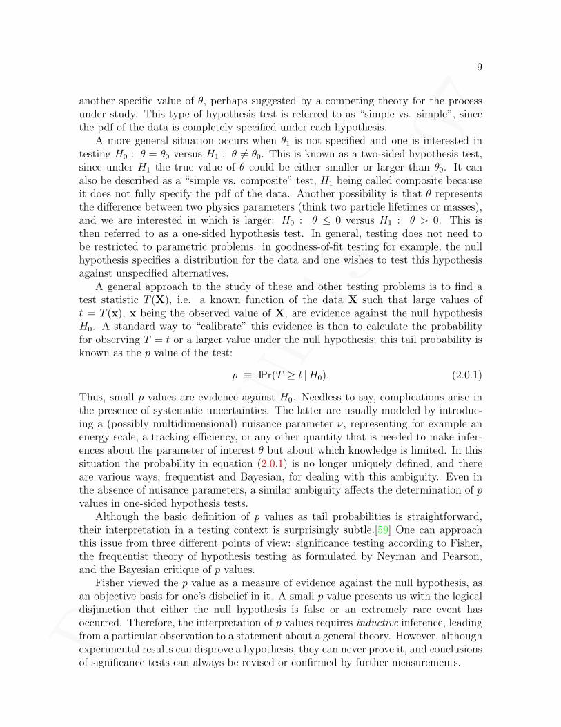
A more general situation occurs when θ1 is not specified and one is interested intesting H0 : θ = θ0 versus H1 : θ 6= θ0. This is known as a two-sided hypothesis test,since under H1 the true value of θ could be either smaller or larger than θ0. It canalso be described as a “simple vs. composite” test, H1 being called composite becauseit does not fully specify the pdf of the data. Another possibility is that θ representsthe difference between two physics parameters (think two particle lifetimes or masses),and we are interested in which is larger: H0 : θ ≤ 0 versus H1 : θ > 0. This isthen referred to as a one-sided hypothesis test. In general, testing does not need tobe restricted to parametric problems: in goodness-of-fit testing for example, the nullhypothesis specifies a distribution for the data and one wishes to test this hypothesisagainst unspecified alternatives.

A general approach to the study of these and other testing problems is to find atest statistic T (X), i.e. a known function of the data X such that large values oft = T (x), x being the observed value of X, are evidence against the null hypothesisH0. A standard way to “calibrate” this evidence is then to calculate the probabilityfor observing T = t or a larger value under the null hypothesis; this tail probability isknown as the p value of the test:

p ≡ IPr(T ≥ t |H0). (2.0.1)

Thus, small p values are evidence against H0. Needless to say, complications arise inthe presence of systematic uncertainties. The latter are usually modeled by introduc-ing a (possibly multidimensional) nuisance parameter ν, representing for example anenergy scale, a tracking efficiency, or any other quantity that is needed to make infer-ences about the parameter of interest θ but about which knowledge is limited. In thissituation the probability in equation (2.0.1) is no longer uniquely defined, and thereare various ways, frequentist and Bayesian, for dealing with this ambiguity. Even inthe absence of nuisance parameters, a similar ambiguity affects the determination of pvalues in one-sided hypothesis tests.

Although the basic definition of p values as tail probabilities is straightforward,their interpretation in a testing context is surprisingly subtle.[59] One can approachthis issue from three different points of view: significance testing according to Fisher,the frequentist theory of hypothesis testing as formulated by Neyman and Pearson,and the Bayesian critique of p values.

Fisher viewed the p value as a measure of evidence against the null hypothesis, asan objective basis for one’s disbelief in it. A small p value presents us with the logicaldisjunction that either the null hypothesis is false or an extremely rare event hasoccurred. Therefore, the interpretation of p values requires inductive inference, leadingfrom a particular observation to a statement about a general theory. However, althoughexperimental results can disprove a hypothesis, they can never prove it, and conclusionsof significance tests can always be revised or confirmed by further measurements.

Dra

ftJu

ne13

,20

07


In contrast with Fisher, frequentists are mainly concerned about long-term errorprobabilities, either incorrectly rejecting the null hypothesis H0 (Type I error), or in-correctly accepting it (Type II error). The standard frequentist test procedure consistsin selecting a Type I error α and delimiting a critical region of sample space that hasprobability α of containing the data under H0. In order to avoid bias, this constructionmust be done in advance of looking at the data. The null hypothesis is then rejectedif the data falls in the critical region. In the simplest case the critical region can berepresented as T ≥ tα, where T is a test statistic and tα a constant that depends on α.It is easy to see that the statement t ≥ tα can be rewritten as p ≤ α, where p is the pvalue defined in equation (2.0.1). The usefulness of the frequentist test procedure thendepends on whether the relevant p value is exact, conservative, or liberal:

p exact ⇔ IPr(p ≤ α |H0) = α,p conservative ⇔ IPr(p ≤ α |H0) < α,p liberal ⇔ IPr(p ≤ α |H0) > α.

These labels obviously depend on α, so that it is in principle possible for a p valueto be conservative for some values of α and liberal for others. In a large number ofindependent tests using the same α and for which H0 is true and the p value everywhereexact, the fraction of tests that reject H0 will tend to α as the number of tests increases.On the other hand, if the p value is conservative or liberal, then the actual Type-I errorrate of the test will be smaller or larger, respectively, than stated. While it is clear thatunderstating the Type-I error rate is undesirable, overstating it can be bad too, as itis usually accompanied by a reduction in power, i.e. in the ability to detect the truthof an alternative hypothesis. This being said, conservatism is often unavoidable, eitherbecause the test statistic is discrete or because of the presence of nuisance parameters.

The notions of conservatism and liberalism are also important in significance testing,although their respective dangers are of a different nature. Indeed, a conservative pvalue is dangerous because it may give one too much confidence in a bad model, whereasa liberal p value, by forcing a search for plausible alternative models more often thannecessary, is less likely to lead to bad inferences.

The difference between hypothesis and significance testing tends to be blurred bypractitioners, and yet it is an important one. Significance tests tell us which experi-mental results are interesting, namely those for which p is less than some threshold.However, the relation between this threshold and a long-term error rate, the focus offrequentist inference, is irrelevant to the evidential character of p. On the other hand,hypothesis tests are predicated on the assumption of repeated testing and are thereforebest suited for problems of quality control, such as selecting a sample of good qualityelectron candidates in a particle physics experiment. In a sense the test criterion pre-sented above, p ≤ α, is very misleading, since it compares two completely unrelatedconcepts, a measure of evidence p and a long-term error rate α. The only correctinterpretation of that inequality is as a clumsy rephrasing of the statement that theobservation lies in the critical region, t ≥ tα. In a hypothesis test setting it wouldmake no sense to report both α and p since the only valid error rate is α. Similarly, in

Dra

ftJu

ne13

,20

07

2.1 The choice of null hypothesis 11

significance testing it would be pointless to report an error probability in addition top since the former does not characterize the evidence against H0 in any way.

We now turn to the Bayesian use of p values. A Bayesian’s primary interest is notin the behavior of a test procedure under a large number of replications, but ratherin the direct evaluation of hypothesis probabilities. In many situations, p values tendto underestimate hypothesis probabilities, leading to conflicts with Bayesian inferences(see section 3). However, most pragmatic Bayesians are willing to consider p valuesas “exploratory tools” or “measures of surprise”[6], capable of indicating that a givenhypothesis provides an inadequate description of the data and that more plausiblealternatives should be investigated. From this point of view, the conflict is mainlyan issue of p value calibration. A more fundamental standpoint is that the evidenceprovided by p values is based not only on the data observed, but also on more ex-treme data that were not observed. Inferences derived from p values therefore violatethe likelihood principle, insofar as the form of the likelihood function itself is beyondsuspicion.2 A more moderate point of view is that p values are just a computationalsummary of the extremeness of the data with respect to model expectations, and thata more informative approach would consist in plotting the observed data on top of anappropriate reference distribution.[50] This is one possible interpretation of the prior-and posterior-predictive formulations of model assessment in the Bayesian paradigm(see sections 4.7 and 4.8 for details).

In any case, Bayesians have developed their own, more orthodox measures of sur-prise, some of which are based on concepts from information theory (see section 3.7).Unfortunately these other measures are far less popular than p values, and the lattercertainly seem destined to remain part of the statistical toolbox of many scientists forthe foreseeable future.

As with other statistical techniques, non-Bayesian uses of p values can benefit fromcombination with Bayesian methods, especially in the area of nuisance parameter elim-ination. This aspect of p values will be examined in section 4.

2.1 The choice of null hypothesis

In most experiments the null hypothesis is easily identified. A typical situation mightinvolve a distribution of observed data that depends on a parameter θ, and we areinterested in a particular value θ0 of θ. In testing θ = θ0 versus θ 6= θ0, only the first ofthese hypotheses fully specifies a pdf for the data, allowing the calculation of a p value.The null hypothesis must therefore be H0 : θ = θ0. In a one-sided test however, sayθ ≤ θ0 versus θ > θ0, neither hypothesis fully specifies the data pdf. One possibilityin this case is to calculate the p value as a function of θ and maximize it over the θregion defined by the null hypothesis. If this recipe works equally well on both sides of

2There is a large area of statistical testing methodology, known as model checking, where the objectof the test is the family of pdf’s describing the data, rather than just a parameter labeling that family.In this case the form of the likelihood function itself is uncertain and the likelihood principle cannotbe invoked.

Dra

ftJu

ne13

,20

07


θ0, additional considerations are needed to decide which hypothesis should be the null.The same issue affects the testing of simple versus simple hypotheses.

An example from high-energy physics will help illustrate some of the ideas involved.An alternative to the standard model of particle physics postulates that the mass ofthe top quark is above 230 GeV/c2, and that the so-called top events observed by theTevatron experiments are really due to an exotic quark of charge Q = −4/3 at thereported mass of ∼ 175 GeV/c2. [22] Furthermore, it is known that the standard andexotic models explain all other electroweak data equally well. One way to test theexotic model is to measure the quark charge in the observed events, which is Q = 2/3if the standard model is correct. Which hypothesis should be the null, Q = 2/3 orQ = −4/3? The temptation may be to choose the latter, because a small p valueunder the exotic model would allow the experimenter to claim rejection of that model“at the observed significance level p”. Consider the following however. The exoticmodel is more complex than the standard model since it contains (at least) one morequark. So, even though both models explain all other data equally well, the exoticmodel has a priori less explanatory power because it requires more parameters. From ascientific point of view we prefer the more parsimonious standard model, and thereforeneed to control the risk of incorrectly rejecting it. This can only be achieved by choosingthe null hypothesis to be the standard model (Q = 2/3) and selecting a small value forthe threshold α. If one adopts Neyman’s frequentist point of view, one should consideras the null hypothesis “the one by which the errors of the first kind are of greaterimportance than those of the second.”[75]

The above argument is particularly important in situations where the data lackpower to discriminate between the two hypotheses. In the context of the top chargeexample, the p value against the exotic model would then likely be as large as the pvalue against the standard model. In this case it is clearly better to fail to reject thestandard model than to fail to reject the exotic model.

If one really has no a priori grounds for preferring one hypothesis over the other, amore natural option is to calculate a likelihood ratio or Bayes factor (see section 3.7).

2.2 The σ scale for p values and the 5σ discovery threshold

Very small p values have little intuitive appeal in terms of how far the observation isfrom the bulk of the distribution. For example, a factor of 10 change in the p valueusually corresponds to a larger shift of the observation when the latter is close to thebulk than when it is far in the tail. To compensate for this nonlinearity, physicistsconventionally map an observed p value to the corresponding number Nσ of standarddeviations a standard normal variate would have to be from zero for the probabilityoutside ±Nσ to equal p:

p = 2

∫ +∞

+Nσ

dxe−x2/2

√2π

= 1 − erf(Nσ/

√2), (2.2.1)

Dra

ftJu

ne13

,20

07

2.2 The σ scale for p values and the 5σ discovery threshold 13

where erf(x) is the standard error function:

erf(x) =2√π

∫ x

0

e−t2 dt. (2.2.2)

Table 1 illustrates the σ scale derived from equation (2.2.1) for a few simple cases. We

Nσ p Nσ p

1 3.17× 10−1 3.89 0.00012 4.55× 10−2 3.29 0.0013 2.70× 10−3 2.58 0.014 6.33× 10−5 1.96 0.055 5.73× 10−7 1.64 0.16 1.97× 10−9 1.28 0.2

Table 1: Correspondence between p values and numbers of σ for some simple examples.

emphasize that this procedure of referencing a p value to a Gaussian distribution isjust a convention. Interpreted literally, it could be very misleading if the observationsare not truly Gaussian. For example, an observation corresponding to a p value of5.73×10−7, while only 5σ in the tail of a Gaussian distribution, is more than 14σ awayin the tail of an exponential distribution!

The factor of two in front of the integral in equation (2.2.1) guarantees that Nσ isalways positive, even when p > 1/2. It is sometimes suggested that this factor shouldbe removed in one-sided problems such as those involving Poisson statistics. This isa needless complication. As noted above, the σ scale for p values is a convention,and conventions are better kept as general as possible. If two experiments use differentmethods to measure the same effect, one based on a one-sided statistic and the other ona two-sided statistic, comparisons between the measurement results should not dependon how one chooses to represent p values.

The threshold for discovery in high energy physics is usually set at 5σ, which mayseem considerably stricter than standard practice in some other sciences. Nevertheless,after comparing the evidence provided by p values with that provided by lower boundson Bayes factors, reference [10] argues that the “commonly perceived” rule of thumbfor interpreting p values should be replaced by a more stringent one:

p Value Interpretation in terms of evidence against H0

Common rule Revised rule

Nσ = 1 Mild NoneNσ = 2 Significant MildNσ = 3 Highly significant SignificantNσ = 4 Overwhelming Highly significant

Dra

ftJu

ne13

,20

07


with the caveat that even the revised rule may overstate the evidence againstH0. Ignor-ing this important caveat, a 5σ effect would be considered overwhelmingly significantunder the revised rule. Whatever one may think of this, there are several additionalreasons for imposing a high discovery standard in high energy physics:

1. P value calculations are often based on parameter estimates whose uncertaintiesare incorrectly assumed to be Gaussian way out in the tails of the distribution.This assumption of Gaussian scaling is typically made when computing p valuesby the Monte Carlo method.

2. Systematic effects are not always easy to identify, let alone to model and quantify.In fact, a null hypothesis is almost never exactly true. The modeling of hypothe-ses in high energy physics requires Monte Carlo simulations of non-perturbativeprocesses that can only be done approximately. Given a large enough data sam-ple, the resulting deviations from exactness will almost certainly lead to small pvalues, regardless of the truth or falsity of the underlying physical theory.

3. Even when systematic effects are correctly identified and understood, the eval-uation of their magnitude often involves an additional uncertainty (e.g. due toMonte Carlo statistics), which is either ignored or simply added in quadratureto the estimated magnitude. However, this uncertainty on an uncertainty mayaffect more than just the size of the original uncertainty, by distorting the veryshape of the resulting distribution of uncertainties. As an example of how thismay come about, consider the estimation of the mean µ of a Gaussian popula-tion. If the true standard deviation σ is known, a 68.27% confidence interval onµ is given by x ± σ/

√n, where n and x are the sample size and mean. More-

over, confidence intervals with 95.45% and 99.73% coverage can be obtained bysimply doubling, respectively tripling the length of the standard interval. On theother hand, if σ must be estimated by the sample standard deviation s, then the68.27% confidence interval becomes wider, namely x ± t0.84 s/

√n, where t0.84 is

the 84th percentile of Student’s t distribution. Furthermore, the Gaussian scalinglaw no longer applies, and doubling the interval length yields less than 95.45%coverage.

4. Large sample sizes are becoming more common in high energy physics. As shownin section 3.3.3, when compared with Bayesian measures of evidence, p valuestend to over-reject the null hypothesis as the sample size increases, and thiseffect is unrelated to the inexactness of null hypotheses mentioned previously.

5. The “look-elsewhere” effect: in some data analysis strategies one looks in severalplaces before finding an unexpected observation somewhere, and it is not alwayseasy to quantify the resulting dilution of significance.

6. The credibility of major HEP experiments is at stake. This means that one maybe interested in the expected fraction Q of false discoveries in the set of claimed

Dra

ftJu

ne13

,20

07

2.3 A simple numerical example 15

discoveries. Given a significance threshold α, Nt true null hypotheses tested,and Nc claimed discoveries, one has Q = αNt/Nc, a number which can be muchlarger than α if Nt is large. Unfortunately Nt is unknown, and therefore so is Q.As shown in Ref. [91] however, it is possible to compute an upper bound on Q,namely Qmax = [(N/Nc) − 1]/[(1/α) − 1], where N is the total number of tests.Suppose for example that one of the LHC experiments makes 1000 searches fornew physics in the course of its lifetime, and that it ends up with 10 discoveryclaims. If these discoveries are based on a 3σ significance threshold, Qmax = 27%,not a very reassuring constraint. On the other hand, at the 5σ level one findsQmax = 0.0056%.

7. It is sometimes necessary to consider one’s prior degree of belief in the nullhypothesis.[69] In a test of the law of energy conservation for example, priorbelief in the validity of that law would be very strong, and the rejection thresholdwould be set very high, perhaps even higher than 5σ, independently of the otherreasons for a high threshold.

It is clear that some of the above arguments could be circumvented by a more carefulstudy of systematic effects and analysis strategy. In any case, many statisticians willcaution against too high a discovery threshold, on the grounds that the fundamentalassumption of experimental high energy physics — that our observations are Poissondistributed — is not exact. The final event samples used in physics analyses resultfrom applying very stringent selection cuts on a very large number of collision events.Thus, the underlying statistical process is actually binomial with sample size N andprobability of success p. In the limit where N → ∞ and p → 0 in such a way thatthe product pN remains constant, the binomial distribution becomes Poisson withmean λ = pN . [21, pg. 93-94] For large N and small p this is only an approximation,albeit a good one. The validity of the binomial assumption itself is rooted in theessential randomness of quantum processes and is therefore rarely questioned. As aresult, investigations of the validity of the Poisson hypothesis have not been donein accelerator settings, in contrast with experiments involving radioactive decay andbackground radiation. [29]

2.3 A simple numerical example

The recent observation by the CDF Collaboration of a resonance in the J/ψπ+π−

mass spectrum near M = 3872 MeV/c2 [2] provides an interesting statistical challengedue to the sheer magnitude of its significance. Indeed, the significance quoted in thePRL [2], 11.6 standard deviations, is too small a probability to be verified with thehelp of Monte Carlo pseudo-experiments. One must therefore rely on testing methodsthat involve statistics with known distributions and that are simple enough to becomputable by numerical quadrature. The same comment applies to methods forincorporating systematic uncertainties, the usual technique of “Monte Carlo smearing”being impractical. Although systematic uncertainties are not a major concern in the

Dra

ftJu

ne13

,20

07


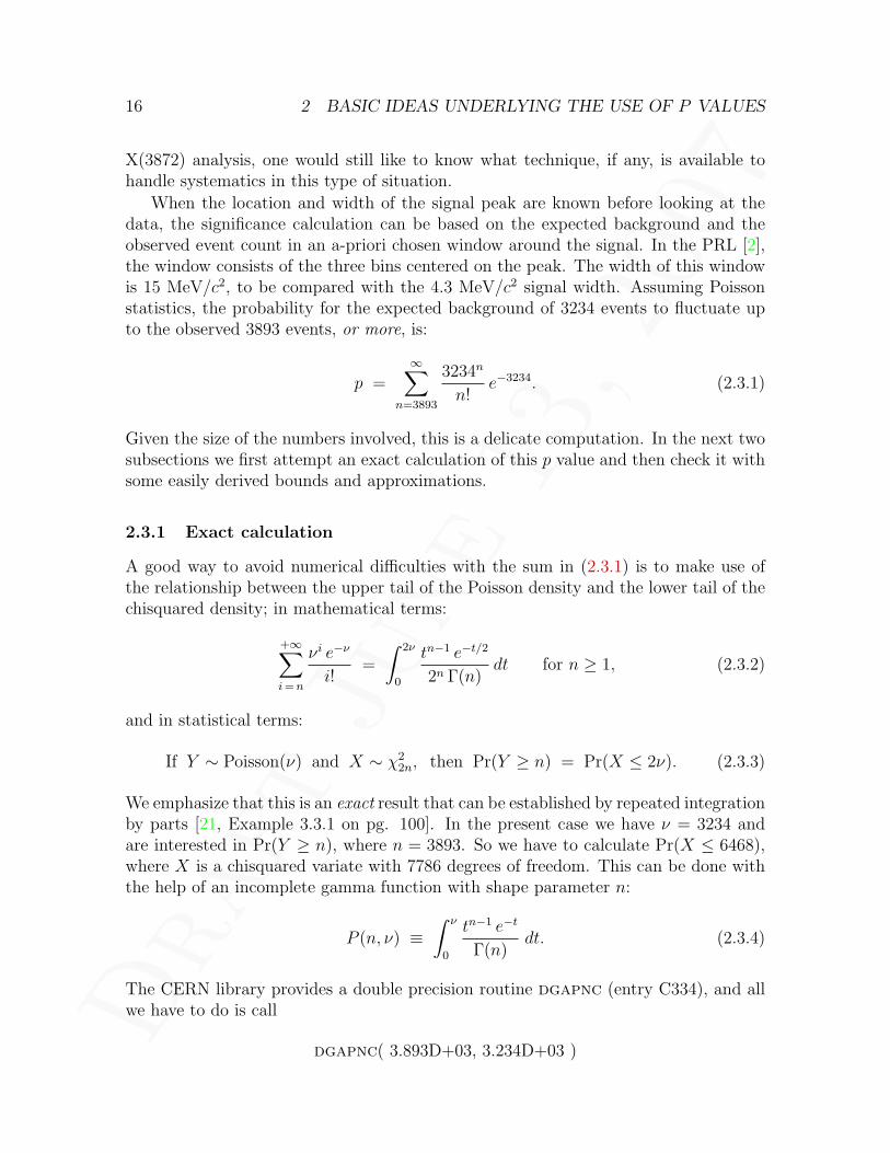
X(3872) analysis, one would still like to know what technique, if any, is available tohandle systematics in this type of situation.

When the location and width of the signal peak are known before looking at thedata, the significance calculation can be based on the expected background and theobserved event count in an a-priori chosen window around the signal. In the PRL [2],the window consists of the three bins centered on the peak. The width of this windowis 15 MeV/c2, to be compared with the 4.3 MeV/c2 signal width. Assuming Poissonstatistics, the probability for the expected background of 3234 events to fluctuate upto the observed 3893 events, or more, is:

p =∞∑

n=3893

3234n

n!e−3234. (2.3.1)

Given the size of the numbers involved, this is a delicate computation. In the next twosubsections we first attempt an exact calculation of this p value and then check it withsome easily derived bounds and approximations.

2.3.1 Exact calculation

A good way to avoid numerical difficulties with the sum in (2.3.1) is to make use ofthe relationship between the upper tail of the Poisson density and the lower tail of thechisquared density; in mathematical terms:

+∞∑i = n

νi e−ν

i!=

∫ 2ν

0

tn−1 e−t/2

2n Γ(n)dt for n ≥ 1, (2.3.2)

and in statistical terms:

If Y ∼ Poisson(ν) and X ∼ χ22n, then Pr(Y ≥ n) = Pr(X ≤ 2ν). (2.3.3)

We emphasize that this is an exact result that can be established by repeated integrationby parts [21, Example 3.3.1 on pg. 100]. In the present case we have ν = 3234 andare interested in Pr(Y ≥ n), where n = 3893. So we have to calculate Pr(X ≤ 6468),where X is a chisquared variate with 7786 degrees of freedom. This can be done withthe help of an incomplete gamma function with shape parameter n:

P (n, ν) ≡∫ ν

0

tn−1 e−t

Γ(n)dt. (2.3.4)

The CERN library provides a double precision routine dgapnc (entry C334), and allwe have to do is call

dgapnc( 3.893D+03, 3.234D+03 )

Dra

ftJu

ne13

,20

07

2.3 A simple numerical example 17

(Note that the relationship between the chisquared and incomplete gamma involvesfactors of two that conveniently cancel those occurring in the relationship between thePoisson and chisquared.) The result is:

1.640× 10−29.

How can we check such a small number? An obvious possibility is to try the Gaus-sian approximations to the Poisson and chisquared, since the Poisson mean and thechisquared number of degrees of freedom are so big. Of course we are looking way outin the tails, so we have to be careful.

2.3.2 Bounds and approximations

Writing ν and n0 for the expected and observed numbers of events, respectively, wehave:

1. Gaussian approximations to the Poisson:One approach is based on the fact that

Z1 ≡ n0 − ν√ν

(2.3.5)

is approximately standard normal. We find Z1 = 11.588, corresponding to aone-sided tail probability of 2.365× 10−31.

A slightly improved calculation uses the property that if Y ∼ Poisson(ν), then√Y is approximately normal with mean

√ν and standard deviation 1/2. Thus

the variableZ ′1 ≡ 2 (

√n0 −

√ν) (2.3.6)

is approximately standard normal. For the X(3872) analysis we find Z ′1 = 11.051,corresponding to a one-sided tail probability of 1.080× 10−28.

2. Gaussian approximation to the chisquared:A chisquared with 2n0 degrees of freedom is approximately Gaussian with mean2n0 and variance 4n0. With the above relationship (2.3.3) between Poisson andchisquared we therefore have that

Z2 ≡ n0 − ν√n0

(2.3.7)

is approximately standard normal. Now we find Z2 = 10.562, corresponding to aone-sided tail probability of 2.237× 10−26.

3. Bounds on the correct p value:A simple modification of the previous two approximations provides bounds onthe correct p value. First, it can be shown that the upper tail of a Gaussian withmean ν−1/2 and variance ν is everywhere below the upper tail of a Poisson with

Dra

ftJu

ne13

,20

07

18 3 PROPERTIES AND INTERPRETATION OF P VALUES

mean ν. Similarly, the lower tail of a Gaussian with mean 2n0 − 2 and variance2×(2n0−2) is everywhere above the lower tail of a chisquared with 2n0 degrees offreedom. In these statements, the upper (lower) tails are assumed to start (end)at the maximum of the distribution. The correct “number of σ’s” is thereforebounded by Z ′′1 and Z ′2, where:

Z ′′1 ≡ n0 − (ν − 1/2)√ν

= 11.597 (2.3.8)

Z ′2 ≡ n0 − 1− ν√n0 − 1

= 10.547 (2.3.9)

or equivalently:

2.134× 10−31 < pcorrect < 2.615× 10−26. (2.3.10)

The dgapnc result satisfies this constraint.

4. Wilson and Hilferty’s Gaussian approximation to the chisquared:This even better approximation to a chisquared with k degrees of freedom statesthat [(

χ2k

k

)1/3

+2

9k− 1

]√9k

2(2.3.11)

is approximately standard normal [93, Equation 16.14 on pg. 546]. Applying(2.3.3), this translates into the variable

Z3 ≡

[1 −

(ν

n0

)1/3

− 1

9n0

]√

9n0 (2.3.12)

for Poisson statistics. We find Z3 = 11.216, corresponding to a one-sided tailprobability of 1.705 × 10−29, remarkably close to the dgapnc result. It is in-teresting to note that the Wilson and Hilferty approximation is also very goodfor much smaller numbers of degrees of freedom. A good example is provided byCDF’s 1994 paper describing evidence for the top quark, in which one calculatesthe Poisson probability for observing 12 events or more when the mean is 5.7[1, section VI.B.1]. Neglecting systematic uncertainties, the correct answer is1.414%. Compare this to the Gaussian approximations to the Poisson: 0.416%for Z1 and 1.565% for Z ′1, the Gaussian approximation to the chisquared: 4.994%,and Wilson and Hilferty’s approximation: 1.435%. The latter is clearly superior.

3 Properties and interpretation of p values

The professional statistical community has had an interesting and at times colorfulhistory of discussions on the subject of p values. The latter were initially popularized

Dra

ftJu

ne13

,20

07

3.1 P values versus Bayesian measures of evidence 19

by Fisher, but the subsequent development of the Neyman-Pearson theory of hypothesistesting, by shifting the focus from p values to fixed-level tests, generated a great dealof confusion and misunderstanding about the basic concepts.[59] Here is a list of someof the more common misinterpretations of p values:

• The p value is the probability of the null hypothesis.

• One minus the p value is the probability of the alternative hypothesis.

• The p value is the probability of rejecting the null hypothesis when it is in facttrue.

• The p value is the probability that the observed results occurred by chance.

• The p value is the probability that the observed results will replicate.

• If the null hypothesis is true, and we keep testing it on a data sample of increasingsize, it will eventually become impossible to disprove it using p values.

• Small p values indicate that the data is unlikely under the null hypothesis.

All of the above statements are false. The following subsections attempt to clarify themeaning of p values, mainly by showing what they are not.

3.1 P values versus Bayesian measures of evidence

A popular misunderstanding of p values is that they somehow represent the probabilityof the null hypothesis H0 after the evidence provided by the data has been taken intoaccount. A simple example will illustrate the fallacy of this belief.[69] Consider aparticle identifier for pions, using dE/dx or the Cherenkov ring angle. For simplicity,let us transform the relevant observable into a variate p that is uniform under the pionhypothesis:

f(p |π) = 1 for 0 ≤ p ≤ 1.

With this convention, p is simply the p value under the null hypothesis that a givenparticle is a pion. Next, assume that muons result in the following p distribution:

f(p |µ) = 1 − 0.1× (p− 0.5),

which is not too different from that for pions, since the pion and muon masses are simi-lar, but is slightly more peaked at small p. Let ππ (πµ) be the fraction of pions (muons)in the sample. These fractions can be interpreted as frequentist prior probabilities fora particle to be a pion or a muon. The posterior pion probability is then:

IPr(π | p) =ππ f(p |π)

ππ f(p |π) + πµ f(p |µ)=

[1 +

πµ

ππ

1

B

]−1

,

Dra

ftJu

ne13

,20

07


where B ≡ f(p |π)/f(p |µ) is the likelihood ratio or Bayes factor in favor of the pionhypothesis. In a sample of particles with equal numbers of pions and muons, theposterior probability for a particle with p ∼ 0.1 to be a pion will be 1/2.04, whichis quite different from 0.1. With a perhaps more realistic particle composition of 100times more pions than muons, that probability will be 100/101.04, even more differentfrom the p value of 0.1.

There is a substantial amount of literature on the relationship between p valuesand posterior hypothesis probabilities (see [10, 20] and references therein). A majorissue is the choice of priors for the Bayesian side of this comparison, since p values areindependent of priors and may therefore appear more objective. One possible approachis to compare a given p value to the smallest posterior hypothesis probability that canbe obtained by varying the prior within some large, plausible class of distributions.This is the approach whose results we will summarize in the remainder of this section.It is instructive to study separately one-sided and point-null hypothesis tests.

For the one-sided case, reference [20] considers the test H0 : θ ≤ 0 versus H1 : θ > 0,based on observing X = xobs, where X has a location density f(x − θ). The densityf is assumed to be symmetric about zero and to have monotone likelihood ratio. Thefollowing classes of priors are used:

• ΓS = {all distributions symmetric about 0};

• ΓUS = {all unimodal distributions symmetric about 0};

• Γσ(g) = {πσ : πσ(θ) = g(θ/σ)/σ, σ > 0},

where g(θ) is any bounded, symmetric, and unimodal density. The class Γσ(g) basicallyconsists of all scale transformations of g; a good example of the latter would be anormal density with mean zero. Assuming that xobs > 0, theorems can then be provedabout the relation between the observed p value pobs and the infimum of the posteriorprobability of H0 over a given class of priors:[20]

infπ∈ΓUS

IPr(H0 |xobs) = pobs

infπσ∈Γσ(g)

IPr(H0 |xobs) = pobs

infπ∈ΓS

IPr(H0 |xobs) ≤ pobs

These results, especially the first two, are quite remarkable. They seem to imply areconciliation between p values and objective Bayesian measures of evidence. Unfor-tunately, as we will indicate next, this agreement does not generalize to other types oftesting problem.

For the point-null problem, reference [10] considers the test H0 : θ = θ0 versusH1 : θ 6= θ0, based on observing X = (X1, . . . , Xn), where the Xi are independent andidentically distributed (iid) according to a normal distribution, N (θ, σ2), with varianceσ2 known; the usual test statistic is T (X) =

√n |X − θ0|/σ. The prior is of the form

Dra

ftJu

ne13

,20

07

3.2 P values versus frequentist error rates 21

π(θ) = π0 if θ = θ0, and π(θ) = (1 − π0) g(θ) if θ 6= θ0, where g(θ) belongs to one ofthe classes:

• GA = {all distributions};

• GS = {all distributions symmetric about θ0};

• GUS = {all unimodal distributions symmetric about θ0}.

The following theorems are then proved:

For tobs > 1.68 and π0 =1

2: inf

g∈GA

IPr(H0 |xobs)

pobs tobs

>

√π

2∼= 1.253

For tobs > 2.28 and π0 =1

2: inf

g∈GS

IPr(H0 |xobs)

pobs tobs

>√

2π ∼= 2.507

For tobs > 0 and π0 =1

2: inf

g∈GUS

IPr(H0 |xobs)

pobs t2obs

> 1

These inequalities imply that p values are usually quite a bit smaller than variouslower bounds on the posterior probability of the null hypothesis, i.e. p values tendto exaggerate the evidence against H0. Although this conclusion differs from the oneobtained for the one-sided study, one can argue that point-null testing is actually themore common problem in high energy physics. When testing a new physics theoryagainst the standard model for example, one can often identify a parameter θ thattakes a particular value θ0 if no new effect is present. Thus one is really interested intesting θ = θ0 rather than θ ≤ θ0. In any case, the wider implication from both theone-sided and point-null studies is that there is no uniform calibration for p values.Their interpretation depends on the type of problem studied. Later we will show thatit also depends on the sample size.

3.2 P values versus frequentist error rates

One sometimes hears statements to the effect that a reported p value pobs is the proba-bility for rejecting the null hypothesis H0 when it is in fact true. These allegations areusually justified by considering a long sequence of measurements in which H0 is alwaystrue, and where one rejects H0 whenever the observed p value is less than pobs; in thissetup the fraction of wrong decisions about H0, i.e. the frequentist Type I error rate,tends to pobs in the long run. Of course this reasoning only works if the error rate wasset to pobs before performing all the measurements in the ensemble. The problem thenis that for the real-life experiment the value of pobs was not known before the test, andcan therefore not be identified with an error rate. One might perhaps hope to save theerror rate interpretation of p values by only requiring that their expectation value oversome ensemble be equal to the nominal error rate α.[37] This is similar to a frequentistconfidence interval construction, where one only requires that the individual interval

Dra

ftJu

ne13

,20

07


coverages, which are 0 or 1, average to the nominal coverage (for example 68%). Un-fortunately the expectation value of all the p values in an ensemble of tests of a correcthypothesis H0 is 1/2, and the expectation value of all the p values that result in theincorrect rejection of H0 is α/2. Clearly, this line of reasoning cannot lead to a consis-tent interpretation of p values as error rates. Another possibility would be to interpretthe observed p value as the smallest Type I error rate at which one could reject thenull hypothesis. While true in principle, this interpretation seems quite irrelevant: onewould much rather know the largest error rate one is likely to encounter.

It is illuminating to pursue this comparison of p values and frequentist error ratesa little further.[84] Imagine a large ensemble of hypothesis tests with a known fractionof true null hypotheses, and consider an arbitrary p value p0, small enough to lead torejection of the tested hypotheses. What is then the error rate for p values in a smallneighborhood of p0? To fix ideas it will be useful to study a concrete example.

Suppose that we are working with an electron beam that is contaminated by pions.We wish to test each particle in the beam to determine whether or not it is an electron.The apparatus we use for this purpose produces a measurement X with the followingdistribution:

X ∼ N (x;µe, σe) if particle is an electron,

∼ N (x;µπ, σπ) if particle is a pion,

where N (x;µ, σ) is a Gaussian distribution in x, with mean µ and width σ, and weassume that µπ > µe. We reject the null hypothesis:

H0 : particle is an electron,

whenever the observed value of X is larger than or equal to a critical value xc. In termsof the p value

p ≡∫ +∞

x

N (y;µe, σe) dy, (3.2.1)

we reject H0 if p ≤ α, where α and xc are related by:

α =

∫ +∞

xc

N (y;µe, σe) dy =1

2

[1 + erf

(µe − xc√

2σe

)].

With these definitions our electron selection cut has an efficiency of 1 − α. Considernow all the particles for which we measure a p value between po−δ and po, where δ is asmall number and po ≤ α. As we reject H0 for all these particles, we would like to knowthe fraction of true electrons among them, i.e. the Type I error rate corresponding topo. Let xo and xo + η be the values of X corresponding to po and po − δ respectively,by applying equation (3.2.1). Letting Ne (Nπ) be the total number of electrons (pions)

Dra

ftJu

ne13

,20

07

3.2 P values versus frequentist error rates 23

in the beam, the fraction of electrons with a p value between po − δ and po is then:

εI(po) =

∫ xo+η

xo

dy NeN (y;µe, σe)∫ xo+η

xo

dy NeN (y;µe, σe) +

∫ xo+η

xo

dy Nπ N (y;µπ, σπ)

,

≈ NeN (xo;µe, σe)

NeN (xo;µe, σe) + Nπ N (xo;µπ, σπ),

=

[1 +

Nπ

Ne

N (xo;µπ, σπ)

N (xo;µe, σe)

]−1

.

Next, replacing N (xo;µπ, σπ) by its maximum, we obtain a lower bound on the TypeI error rate corresponding to po:

εI(po) ≥[1 +

Nπ

Ne

1√2π σπ N (xo;µe, σe)

]−1

.

Or, mapping xo into po with the help of equation (3.2.1):

εI(po) ≥[1 +

Nπ

Ne

σe

σπ

e

[erf−1(2po − 1)

]2 ]−1

. (3.2.2)

Table 2 shows some numerical examples of this lower bound for the case Ne = Nπ,σe = σπ. The lower bound is always significantly larger than the p value, again showing

po Lower bound on εI(po) Ratio

0.05 0.21 4.10.01 0.063 6.3

0.0027 0.020 7.65.7× 10−7 7.2× 10−6 12.7

Table 2: Calculation of the lower bound on the Type I error rate given by equation(3.2.2), for a few p values. The last column gives the ratio of the lower bound on theerror rate to the p value.

that p values cannot be relied upon to estimate frequentist error rates. In some senseour testbeam example trivializes this problem. A more educational exercise wouldconsist in looking back over the history of high-energy physics, and making a list of allthe hypothesis tests ever made and for which the truth eventually became known.[12]Suppose that half of the tested hypotheses were in fact wrong. Table 2 then showsthat the fraction of hypotheses that were incorrectly rejected with a p value around5.7× 10−7 is more than 10 times higher than that p value.

Dra

ftJu

ne13

,20

07


To summarize, frequentist error rates are never conditioned on the actual observa-tion, but must be specified before doing the measurement: they are simply predictionson the performance of a procedure. In this context, the only purpose of calculating ap value is to determine what action to take, i.e. accept or reject the null hypothesis.

3.3 Dependence of p values on sample size

The behavior of test procedures as a function of sample size occasionally becomes rele-vant in high energy physics, although the associated issues are rarely acknowledged. Forexample, one might want to compare or combine significances obtained from sampleswith different sizes, or update a search for new physics at regular intervals of integratedluminosity. Sample size affects such procedures in various ways. On a purely mathe-matical level, the law of the iterated logarithm implies that significance levels need tobe adjusted for the way an experiment is conducted. Another aspect relates to the wayp values behave as a function of sample size when compared with other measures ofevidence, such as Bayesian posterior probabilities. Thirdly, in order to be admissible,a strictly frequentist approach to testing constrains the dependence of error rates onsample size. Finally, there is also an issue of “practical” versus statistical significance.

3.3.1 Stopping rules

A typical search strategy in high energy physics is to analyze the collected data atregular intervals to see if new physics effects are emerging as the fluctuations of knownphysics backgrounds stabilize with increasing sample size. An important considerationin this context is that the test statistics used in the search perform a random walkas the data accumulates. It is therefore entirely possible that an interesting effectobserved in a sample of given size disappears with more data. This has implicationsfor the choice of test levels. Consider for example the following search procedure:

1. Select n1 signal-like events from a sample of given integrated luminosity L, cal-culate the expected background b and the corresponding p value p1 ≡ p(b, n).

2. If p1 ≤ α, reject the “background-only” null hypothesis and stop taking data.

3. If p1 > α, collect another sample of integrated luminosity L, extract the numbern2 of signal-like events in the new sample, and update the p value, p2 ≡ p(2b, n1+n2).

4. Stop taking data and reject the null hypothesis if p2 ≤ α.

It is clear that the overall Type I error rate of this procedure is larger than α:

IPr(p1 ≤ α or p2 ≤ α) ≥ α.

In a general procedure with one or more intermediate testing points, maintaining agiven overall Type I error rate requires that one adjust the intermediate test levels as

Dra

ftJu

ne13

,20

07

3.3 Dependence of p values on sample size 25

a function of the overall level, as well as of the number and spacing of the intermediatetests.

The above remarks imply that the calibration of p values depends on the testingstrategy. This dependence also manifests itself with respect to how an experiment isterminated. The classical example of this is an experiment that detects two types ofevents, for example two decay modes of an unstable particle, and is designed to testa particular value for the branching fraction of one of the modes.[37] The probabilitymass function (pmf) of the observations is binomial if the experimenter decides to stopafter observing a given total number of decays, but is negative binomial if the stoppingrule is to wait until a given number of decays of a specific mode have been collected.The p value will of course depend on the form of the pmf.

This discussion of testing strategies raises a new question. Suppose we keep ontaking data and regularly test the null hypothesis. As the sample size increases, isthere any guarantee that the probability for making the correct decision regarding H0

goes to 1? Interestingly, the answer is no, if the test level is kept constant. This is adirect consequence of the law of the iterated logarithm (LIL). The latter applies to anysequence of random variables Xi that are independent and identically distributed withfinite mean µ and variance σ2 6= 0. Consider the partial sums Sn ≡

∑ni=1Xi. The LIL

then states that with probability one the inequality

|Sn − nµ| ≥ σ(1 + δ)√

2n ln lnn

will hold for only finitely many values of n when δ > 0 and for infinitely many values ofn when δ < 0. Therefore, the curve of

√2n ln lnn versus n defines a kind of “boundary

of boundaries” (BoB) for partial sum fluctuations. As the sample size increases, aboundary curve just below the BoB will be crossed infinitely often by these fluctuations,whereas a boundary curve just above the BoB will only be crossed finitely many times.To see the relevance of this for p values, suppose the Xi are all Gaussian with knownσ and we wish to test H0 : µ = µ0 versus H1 : µ 6= µ0. An optimal test statistic forthis test is:

Zn ≡ Sn/n − µ0

σ/√n

,

and the corresponding p value is:

pn = 2

∫ ∞

|Zn|dte−t2/2

√2π

= 1 − erf

(|Zn|√

2

).

Thus, testing pn against a fixed level, say pn ≤ α, is equivalent to testing for |Zn| ≥ cfor some fixed c. According to the LIL however, the event

|Zn| ≥ (1 + δ)√

2 ln lnn (3.3.1)

happens infinitely many times if δ < 0. Therefore, regardless of the choice of thresholdc, |Zn| will eventually exceed it for some n, even if the null hypothesis is true. This

Dra

ftJu

ne13

,20

07


phenomenon is usually referred to as “sampling to a foregone conclusion.” The onlyway to avoid it is to make c a function of n, that increases at a faster rate than theboundary specified by equation (3.3.1). Equivalently, one could keep decreasing thetest level α as a function of n, or correspondingly rescale the p value. This latter optionhas the advantage of being independent of the choice of α. Reference [51] proposes tostandardize p values according to the following rule:

pstan = min

{1

2, p

√N

nstan

}, (3.3.2)

where N is the number of observations used in calculating p and nstan is a standardsample size appropriate for the analysis of interest. This rescaling of p values by

√N

is actually more than sufficient to cancel the effect of the LIL. It has the additionaladvantages of being simple to apply and of bringing p values into closer relationshipwith other measures of evidence (see below).

As shown in ref. [30], the LIL allows many types of refinement of the above rescalingrule. For example, for two-sided tests it is possible to construct n-dependent intermedi-ate test levels such that the overall Type I error probability is controlled, and withouthaving to fix the total sample size in advance. For one-sided tests it is possible toconstruct a procedure that will end in a finite amount of time with the acceptance ofone or the other hypothesis with arbitrarily small error probability.

3.3.2 Effect of sample size on the evidence provided by p values

Suppose two experiments observe an interesting effect for which both obtain the samep value, even though the sample size of the second experiment is 100 times larger thanthat of the first one. An interesting question is whether or not these two experimentsprovide the same evidence for the effect, as the p values indicate, regardless of samplesize.

To illustrate the issues, let the quantity of interest be the mean µ of a Gaussiandistribution with known width σ. The experiment consists in taking n measurementsX1, . . . , Xn of µ and to test H0 : µ = µ0 versus H1 : µ 6= µ0. The likelihood ratio testrejects H0 for large values of

Z ≡ |X − µ0|σ/√n, where X =

1

n

n∑i=1

Xi. (3.3.3)

The p value corresponding to observing Z = z0 ≡√n |x0 − µ0|/σ is:

p = 2

∫ +∞

z0

dze−z2/2

√2π

= 1 − erf(z0/√

2). (3.3.4)

Suppose now that, having chosen a small α prior to the experiment, we find p ≤ α andtherefore reject H0. It is then interesting to set bounds on the true value of µ. If for

Dra

ftJu

ne13

,20

07


example the mean x0 of all n measurements is larger than µ0, one could calculate a βconfidence level lower limit µ` on µ:

µ` = x0 −√

2

nσ erf−1(2β − 1) = µ0 +

√2

nσ[erf−1(1− p)− erf−1(2β − 1)

],

where the second expression on the right was obtained by using equations (3.3.3) and(3.3.4) to express x0 in terms of the p value. This result shows that for a fixed valueof p, the lower limit depends on the sample size n.

For a numerical example we take µ0 = 0, σ = 1, and assume that a first experimentmakes 100 measurements and finds x0 = 0.26, whereas a second experiment makes10000 measurements and finds x0 = 0.026. Both experiments obtain a p value of0.9% and reject H0 at the α = 1% level. Having established that the observationsare unlikely under the null hypothesis, we may wish to know for what other values ofµ this is the case. Or to put it another way, if we were to relax the cutoff α, howmuch additional parameter space would we be excluding, and how does this dependon sample size? One way to answer this question for this particular problem is tocalculate a 90% confidence level lower limit on the true value of µ. This lower limit is0.133 (0.013) for the first (second) experiment. By construction, it can be interpretedas an upper limit on the set of µ values for which the observation is unlikely: even if thetrue value of µ were as high as 0.133, replications of the first experiment would yield Xgreater than its observed value at most 10% of the time. Given that the correspondinglimit for the second experiment is only 0.013, the evidence against µ = 0 is stronger inthe first experiment than in the second.

Two lessons can be drawn from this example. The first one is that, given identicalp values, the evidence coming from a small sample should be considered stronger thanthat coming from a large sample. The second one is that p values by themselves do notprovide a complete picture of the evidence contained in a data sample, and confidenceintervals or limits can provide additional useful information.

3.3.3 The Jeffreys-Lindley paradox

Section 3.1 compared p values with Bayesian measures of evidence. Here we revisitthis comparison in terms of the dependence on sample size.[51] Suppose we make nmeasurements of a quantity X whose distribution is Gaussian with unknown mean µand known width σ. We wish to test H0 : µ = 0 versus H1 : µ 6= 0. The p valueapproach to this problem starts from the test statistic:

Z ≡ |X|σ/√n. (3.3.5)

For an observed value z0 of Z, the p value is then:

p = 2

∫ +∞

z0

dze−z2/2

√2π

= 1 − erf

(z0√2

). (3.3.6)

Dra

ftJu

ne13

,20

07


The Bayesian approach is based on the Bayes factor, which is defined as the factorB01 by which the prior odds in favor of H0 must be multiplied in order to obtain theposterior odds in favor of H0. This factor therefore represents the evidence providedby the data. A simple application of Bayes’ theorem shows that:

B01 =p(x |H0)

p(x |H1).

If the hypotheses are simple, this reduces to the likelihood ratio. In our examplehowever there is one parameter, µ, so that p(x |Hi) (i = 0, 1) is not a likelihood butthe marginal, or predictive probability density of the data:

p(x |Hi) =

∫dµ p(x, µ |Hi) =

∫dµ p(x |µ,Hi) π(µ |Hi),

where p(x |µ,Hi) is the likelihood under Hi and π(µ |Hi) is the prior for µ under Hi.Letting δ(µ) be a point-mass probability at µ = 0 and ϕ(µ) a broad distribution, forexample a normal with mean 0 and large width τ , we set:

π(µ |H0) = δ(µ)

π(µ |H1) = ϕ(µ).

The likelihood under H1 is:

p(~x |µ,H1) =n∏

i=1

e−12

(xi−µ

σ

)2

√2π σ

=e−1

2v2+(µ−x)2

(σ/√

n)2

(√

2π σ)n,

with x ≡∑n

i=1 xi/n and v2 ≡∑n

i=1(xi − x)2/n. The likelihood under H0 can beobtained by setting µ = 0 in the above. The predictive densities are then:

p(~x |H0) =e−1

2v2

σ2/n

(√

2π σ)ne−z2

0/2

∫dµ δ(µ) =

e−1

2v2

σ2/n

(√

2π σ)ne−z2

0/2,

p(~x |H1) =e−1

2v2

σ2/n

(√

2π σ)n

√2π σ√n

∫dµ

e−1

2

(µ−xσ/√

n

)2

√2π σ/

√nϕ(µ) ≈ e

−12

v2

σ2/n

(√

2π σ)n

√2π σ√n

ϕ(0),

where the approximation if valid for large n, in which case the integral is approximatelyequal to ϕ(x), and for τ large enough this is further approximated by ϕ(0). The Bayesfactor is the ratio of the above expressions:

B01 =

√n

ϕ(0)

e−z20/2

√2π σ

.

Consider a situation where the p value of equation (3.3.6) remains fixed as n increases.The value of z0 then also remains fixed, so that the Bayes factor in favor of H0 increases

Dra

ftJu

ne13

,20

07


as√n. This is the Jeffreys-Lindley paradox: at large n, a large value of z0 will cause

the user of p values to reject H0, whereas the Bayesian will not. According to equation(3.3.5), for z0 to remain constant the mean x must decrease as 1/

√n; the Bayesian

analysis sees this decrease as evidence in favor of H0. A simple way to resolve theparadox is to rescale p values by

√n, as in equation (3.3.2).

3.3.4 Admissibility constraints

A common frequentist approach to hypothesis testing is to fix the probability α ofincorrectly rejecting the null hypothesis, and then to find a test procedure that min-imizes the probability β of incorrectly rejecting the alternative hypothesis. It can beshown however, that keeping α fixed regardless of the sample size n is inadmissible, inthe technical sense that it leads one to prefer a test with (α, β) error rates that are notthe smallest achievable.[17] The way this comes about is as follows. Let Tn(α) be theα-significance level test one would apply to a sample of size n, and suppose that theactual sample size is a random number.3 For simplicity, assume that we are dealingwith only two unequal sample sizes, n1 and n2, and that they each have the sameprobability of occurring. A preference for using the same α in both Tn1(α) and Tn2(α)implies a preference for the randomized test T ≡ 0.5Tn1(α) + 0.5Tn2(α) over any testof the form T ′ ≡ 0.5Tn1(α1) + 0.5Tn2(α2), with α1 6= α2. Now, it turns out that α1

and α2 can be chosen in such a way that the overall type I and type II error rates ofT ′ are not larger than the corresponding error rates of T , and at least one error rateis strictly smaller. The test T , based on a fixed α, is therefore inadmissible. A verygeneral theorem then shows that in order to be admissible, the choice of α must besuch that dβn(αn)/dαn is constant as a function of n. This result can also be derivedfrom an expected loss argument. For simple versus simple testing, the implication fromthe theorem is that αn should decrease exponentially fast as a function of sample sizen; for composite alternatives the decrease is much slower, going as 1/

√n. A decrease

in α can of course always be converted into a corresponding increase in the p value ofthe test.

3.3.5 Practical versus statistical significance

In most testing problems in high energy physics, the null hypothesis is not exactly true,due to various small uncertainties and biases that are difficult to take into accountproperly. One has to decide whether or not to spend extra time and effort to quantifyand parametrize these effects so that they can be included in the model used to describethe data. For small to moderate sample sizes, this may indeed not be necessary.However, as the sample size increases, the test will become more and more sensitive tothe inexactness of H0, resulting in smaller and smaller p values. Eventually the nullhypothesis will be rejected even if the underlying physics it is meant to represent is

3Random sample sizes are a common occurrence in high energy physics, so this is not a vacuoussupposition.

Dra

ftJu

ne13

,20

07


true. Ref. [71] proposes a method for taking small but irrelevant discrepancies intoaccount when performing χ2 goodness-of-fit tests on large samples.

3.4 Incoherence of p values as measures of support

The usual application of p values is as measures of surprise, a small p value being anindication that the data does not support the null hypothesis. However, it is sometimestempting to suggest the obverse interpretation: if a p value is large, can it be viewedas a measure of support for the null hypothesis? To fix ideas, consider the simpleproblem of testing the mean µ of a normal density by using the average x of severalmeasurements. For p values to be useful as measures of support, they need to possesssome elementary properties:

1. The farther the data is from the hypothesis to be tested, the smaller the p valueshould be.

2. The farther the hypothesis is from the observed data, the smaller the p valueshould be.

3. If H implies H ′, then anything that supports H should a fortiori support H ′;this is the property of coherence.

It is easy to see that p values satisfy the first two of these requirements. However, theydo not always satisfy the third. Compare for example the following two test situations:

H1 : µ = µ0 versus A1 : µ 6= µ0

H2 : µ ≤ µ0 versus A2 : µ > µ0

Suppose that we observe x > µ0, but with relatively large p values under both H1

and H2. Since H1 implies H2, the property of coherence requires that, as a measureof support, the p value under H1 be smaller than the p value under H2: p1 ≤ p2.This is not the case however, since for one-sided versus point-null hypotheses one hasp2 = p1/2 < p1. Reference [82] has generalized this argument to testing situations ofthe form:

H3 : µ ∈ [a, b] versus A3 : µ 6∈ [a, b], (3.4.1)

and with distributions other than the normal, in particular the exponential, the bino-mial, and the uniform. There are incoherences in all cases.

Note that p values for one-sided tests are generally coherent with each other. How-ever, one-sided tests are just a particular case of the more general “interval” testsdefined above, and for which the p values are not coherent.

3.4.1 The problem of regions paradox

An interesting illustration of the incoherence of p values as measures of support comesup in the so-called problem of regions.[42] This refers to a class of problems where one

Dra

ftJu

ne13

,20

07

3.4 Incoherence of p values as measures of support 31

tries to determine which one of a discrete set of possibilities applies to a continuousparameter vector. Examples familiar in high energy physics include the determinationof the degree of the polynomial used to model a background spectrum in the searchfor a resonance, the estimation of the number of modes in a spectrum, and also somesimultaneous significance tests.

Consider a generic problem where we are trying to determine which one of two re-gions a particular k-dimensional parameter ~µ belongs to. The two regions are separatedby a spherical boundary of known radius θ1:

R1 = {~µ : ‖~µ‖ ≤ θ1}, R2 = {~µ : ‖~µ‖ > θ1}.

Data vectors ~X are assumed to follow a multivariate normal distribution with mean ~µand unit covariance matrix. Suppose now that the observed data vector ~x0 falls intoregion R2. With what confidence can we then assert that ~µ ∈ R2? A possible answerto this question is based on the distance Z between the data ~X and the nearest ~µ not inR2. It is easy to verify that for this problem Z2 equals Wilks’ likelihood ratio statisticfor testing the null hypothesis H0 that µ lies in Rc

2, the complement of R2:

Z2 = −2 ln

[sup~µ∈Rc

2G( ~X; ~µ,1)

sup~µ∈R2G( ~X; ~µ,1)

],

whereG( ~X; ~µ, V ) is a multivariate Gaussian density with mean ~µ and covariance matrixV .4 We quantify our confidence that ~µ lies in R2 by calculating one minus the p valueagainst H0:

q ≡ 1 − p = inf~µ∈Rc

2

IPr(Z ≤ z0) = inf~µ∈Rc

2

IPr(‖ ~X‖ − θ1 ≤ z0)

= inf~µ∈Rc

2

IPr(‖ ~X‖2 ≤ (θ1 + z0)2),

where z0 is the observed value of Z. The statistic ‖ ~X‖2 has a noncentral chisquareddistribution with k degrees of freedom; the above probability reaches its infimum when~µ is on the boundary between R1 and R2, i.e. when the non-centrality parameter ofthe ‖ ~X‖2 distribution equals θ2

1. If we take for example k = 4, θ1 = 5, and ‖~x0‖ = 7,then we find q = 0.9596.

Suppose next that we add a new region R3 to this problem, separated from R2

by another spherical boundary with radius θ2 > θ1. Thus, R2 is reduced to the bandbetween R1 and R3:

R1 = {~µ : ‖~µ‖ ≤ θ1}, R2 = {~µ : θ1 < ‖~µ‖ < θ2}, R3 = {~µ : ‖~µ‖ ≥ θ2}.4The supremum of a function f over a set S is the smallest upper bound on f(x) for x ∈ S; it is

denoted by supS f(x). If the supremum is actually reached by f , it is called the maximum. One cansimilarly define the infimum and minimum of a function.

Dra

ftJu

ne13

,20

07


Assuming that the observed data ~x0 is still in R2, how does the new region affect ourconfidence that ~µ ∈ R2? We can again try to answer this question with the help of thestatistic Z defined above. We now have Z = min{‖ ~X‖ − θ1, θ2 − ‖ ~X‖}, so that:

q = inf~µ∈Rc

2

IPr(Z ≤ z0),

= inf~µ∈Rc

2

IPr(‖ ~X‖ − θ1 ≤ z0 or θ2 − ‖ ~X‖ ≤ z0

),

= 1 − sup~µ∈Rc

2

IPr(‖ ~X‖ − θ1 > z0 and θ2 − ‖ ~X‖ > z0

),

= 1 − sup~µ∈Rc

2

IPr((θ1 + z0)

2 < ‖ ~X‖2 < (θ2 − z0)2).

The ‖ ~X‖2 distribution is again noncentral chisquared with k degrees of freedom, and theprobability reaches its supremum when the non-centrality parameter equals θ2

1. Usingthe same numerical example as previously, and adding a boundary at θ2 = 9.5, we nowfind q = 0.9717. In other words, decreasing the size of the region R2 has increased ourconfidence that µ ∈ R2. As shown in reference [42], this kind of paradoxical behaviordoes not occur with Bayesian methods of assessing confidence.

3.4.2 Rao’s paradox

Suppose we have one observation ~x = (2.06, 2.06) from a bivariate normal distributionwith unknown mean ~µ = (µ1, µ2), unit standard deviations (σ1 = σ2 = 1), and acorrelation coefficient ρ = 0.5. The problem is to test whether the data are consistentwith H0 : ~µ = (0, 0) at the 5% level. This is usually solved with Hotelling’s T 2 test.If Σ denotes the covariance matrix of the data, we find t2 ≡ ~x ′Σ−1~x = 5.658, which issmaller than 5.991, the 0.95 quantile of a χ2

2 distribution. The null hypothesis is there-fore accepted. On the other hand, if we were to test each component of µ separately,we would find that the null hypothesis is rejected, since x2

1 = x22 = 2.062 = 4.244, which

is larger than 3.841, the 0.95 quantile of a χ21 distribution. This incoherence is known

as Rao’s paradox.[15]

3.5 Calibration of p values

Although p values were introduced as a way to calibrate the evidence provided by theobserved value of a test statistic against a given null hypothesis, it is clear from theprevious sections that this calibration is far from perfect. Indeed, it disagrees withBayesian posterior probabilities as well as with frequentist error rates, depends on thestopping rule, and fails to take sample size into account. A correction for the last twoinadequacies was proposed in reference [51] and described in section 3.3.1:

pstan = min

{1

2, p

√N

nstan

}, (3.5.1)

Dra

ftJu

ne13

,20

07

3.6 P values and interval estimates 33

where N is the actual sample size and nstan a standard sample size appropriate for theproblem at hand.

Reference [84] proposes a different calibration, whose aim is to partially reconcile pvalues with Bayesian and frequentist measures. The method is to compute

B(p) = −e p ln(p), (3.5.2)

and interpret the result as a lower bound on the odds (or Bayes factor) of H0 to H1.If a type-I frequentist error probability is preferred, the calibration is:

α(p) =1

1 + 1−e p ln(p)

. (3.5.3)

This expression can also be interpreted as the posterior probability of H0 that wouldresult from using the Bayes factor in (3.5.2) together with the assumption of equal priorprobabilities for H0 and H1. A couple of examples familiar in high energy physics willhelp illustrate this calibration: for a 3σ effect the p value is 0.0027, yielding B = 0.0434(odds of 1 to ∼ 23), and α = 0.0416; for a 5σ effect the p value is 5.7 × 10−7, givingα ≈ B = 2.228× 10−5 (odds of 1 to ∼ 45000).

The calibrations (3.5.2) and (3.5.3) assume that the p value is uniform under the nullhypothesisH0 and that the latter is of the point-null type. The general recommendationof [84] is that these calibrations should only be used in the absence of an explicitalternative hypothesis. Objective Bayesian or conditional frequentist procedures shouldbe applied whenever the alternative is specified.

3.6 P values and interval estimates

We already argued in section 3.3.2 that the evidence provided by p values may needto be complemented by an interval estimate of the quantity of interest. Aside fromhelping to assess evidence, intervals yield useful information regardless of whether ornot a discovery is claimed. If no such claim is made, a carefully chosen lower or upperlimit constitutes a useful post-data measure of the sensitivity of the measurement. Onthe other hand, in case of discovery a two-sided interval provides a plausible range ofmagnitudes for the observed effect.

Another approach is to report the full p value function.[48] For models with alocation parameter θ and a one-dimensional observable X, the p value function isdefined as the integrated probability to the left of the observed data, viewed as afunction of θ.5 If the data is in the right-hand tail of the null distribution, and thisis the tail of interest for testing the null hypothesis θ = θ0, then the standard p valueequals 1 minus the p value function evaluated at θ0. In addition to calculating p values,one can construct confidence intervals at the 1−α level by finding the parameter valuesfor which the p value function equals 1 − α/2 and α/2. Because of these properties

5This definition can be generalized to models that are not exactly of the location type or includenuisance parameters. See Reference [48] for details and further references.

Dra

ftJu

ne13

,20

07


the p value function is sometimes referred to as the “significance function”, or the“confidence distribution function.” It is analogous to the marginal posterior cumulativedistribution function of Bayesian inference. To summarize, by presenting the full pvalue function, one provides a powerful way for the reader to assess both the significanceof the observation and a plausible range of magnitudes for the effect of interest, whethera discovery is claimed or not.

We close this discussion with some caveats about the well-known correspondencebetween hypothesis testing and interval estimation (see for example section 9.2.1 in[21]). As the following example shows, it is not always wise to use confidence intervalsto reject null hypotheses that define a special value for a parameter.[11] Suppose weare measuring an observable X with pdf:

f(x | θ) = (1 + ε) − 4ε |x − θ|, for θ − 1

2≤ x ≤ θ +

1

2.

For small ε, the usual 95% central confidence interval for θ is:

C(x) = [x− 0.475, x+ 0.475].

If θ = 0 is a special value and we observe x = 0.48, the likelihood ratio for testingH0 : θ = 0 is:

f(0.48 | 0)

supθ∈C(0.48) f(0.48 | θ)≥ 1− ε

1 + ε,

which for small ε does not justify rejecting H0. Although this example is somewhatcontrived, the same phenomenon occurs to a lesser degree with other distributions. Inhigh-energy physics we often have a special parameter value to test, corresponding tothe “standard model” value. Calculating a confidence interval is not the best way toquantify the evidence contained in the data against (or in favor of) that special value.

A second caveat is that tests derived from interval constructions tend to have thesame mixture of desirable and undesirable properties as the latter. Suppose for examplethat we obtain a Gaussian measurement x, with unknown positive mean µ and knownwidth σ = 1. The α-level central confidence interval for µ is given by x±

√2σ erf−1(α).

If this interval does not contain the value µ = 0, then we can actually say that µ = 0 isexcluded at the (1− α)/2 level. This is a direct consequence of the way central confi-dence intervals are constructed, which is such that the interval boundaries themselvesare valid confidence limits. In contrast, Feldman-Cousins [46] interval boundaries donot have this property. If we constructed an α-level Feldman-Cousins interval in theabove Gaussian example and it did not contain the value µ = 0, then we would onlybe able to claim that µ = 0 is excluded at the 1 − α level. On the other hand, if weobserved a large negative value for x, then the rather plausible parameter value µ = 0would be excluded by the central interval construction but not by the Feldman-Cousinsone.

Dra

ftJu

ne13

,20

07

3.7 Alternatives to p values 35

3.7 Alternatives to p values

The many defects of p values discussed in the previous sections have led statisticiansto search for alternative measures of surprise with better properties. Some interestingoptions are listed below, in no particular order (see Ref. [6] for a partial review).

1. Bayesian significance tests [67]:

Given a parameter θ, a test of the hypothesis that θ = θ0 can be based onthe posterior distribution of θ. One first calculates a β-credibility level posteriorinterval for θ. Then, if θ0 is outside that interval, one can state that the hypothesisθ = θ0 is rejected at the α = 1− β significance level. An exact significance levelcan be defined as the smallest α (largest β) for which θ = θ0 is rejected. There isof course a lot of freedom in the choice of credibility interval. A natural possibilityis to construct a highest posterior density interval, but this depends on the formof the null hypothesis. If we wish to test the hypothesis θ ≤ θ0 for example,then a better approach is to calculate a lower limit θL on θ, and exclude thehypothesis if θ0 < θL. In this case the exact significance level is simply theposterior probability for θ ≤ θ0.

2. Likelihood ratios [79]:

The law of likelihood states that, for two hypothesesH1 andH2, the one that givesgreater probability (or probability density) to observed data xobs is the one that isbetter supported. If one subscribes to that law, the strength of evidence support-ing H1 over H2 is then given by the ratio of densities f(xobs |H1)/f(xobs |H2). Aninteresting quantity is the probability of misleading evidence, i.e. the probabilitythat the likelihood ratio favors one hypothesis when the other is true. There is auniversal bound on this probability:

IPr

[f(xobs |H1)

f(xobs |H2)≥ k

∣∣∣∣H2

]≤ 1

k. (3.7.1)

Although this bound is achievable, it is usually not the strongest bound in largesamples. One can show that, asymptotically, the probability of misleading evi-dence is bounded by Φ(−

√2 ln k), where Φ is the cumulative normal distribution

with zero mean and unit width. In the presence of nuisance parameters, thenumerator and denominator of the likelihood ratio should separately be maxi-mized over them. The resulting ratio of profile likelihoods can then be used as ameasure of evidence, and the resulting probability of misleading evidence is againasymptotically bounded by Φ(−

√2 ln k). It should be noted that this asymptotic

limit is not reached uniformly, i.e. for any sample size there may remain someparameter values for which the bound is exceeded.

3. Relative likelihoods [9, section 4.7.2]:

If x0 is the observed value of a statistic X with distribution density f(x), two

Dra

ftJu

ne13

,20

07


possible measures of surprise are:

m?(x0) ≡ f(x0)

supx f(x), (3.7.2)

m??(x0) ≡ f(x0)

E [f(X)]. (3.7.3)

If f(x) depends on an unspecified parameter ν, one can use the prior-predictivedistribution instead of f(x) in the above definitions. The prior-predictive distri-bution is the integral of f(x | ν)π(ν) over ν, where π(ν) is a suitable prior densityfor ν. A possible disadvantage of relative likelihood measures is their lack of in-variance under non-linear one-to-one transformations of the observation.

4. Lower bounds on Bayes factors:

Bayes factors are a popular Bayesian way for comparing two hypotheses. How-ever, when one or both hypotheses are composite, a proper prior must be elicitedover the relevant parameter space, which is difficult to do in the absence of ob-jective prior information. One way to overcome this problem was described insection 3.1: it consists in minimizing the Bayes factor in support of a null hy-pothesis over a large class of plausible prior densities. Here we summarize theapplication of this technique to chisquared tests of fit.[36] Suppose we have abinned distribution of events, {ni, i = 1, . . . , t}, that we wish to compare toexpectations {Np0

i , i = 1, . . . , t}, where N ≡∑t

i=1 ni. The standard way toproceed is to compute the weighted sum of squares:

SN =t∑

i=1

(ni −Np0i )

2

Np0i

, (3.7.4)

and to evaluate its significance with the p value:

p = IPr(χ2

t−1 ≥ SN

), (3.7.5)

where χ2t−1 is a chisquared variate with t− 1 degrees of freedom. Strictly speak-

ing, this p value is only an approximation to the correct, multinomial p value.Testing the compatibility of binned data with their expectations is equivalent totesting H0 : ~p = ~p 0 versus H1 : ~p 6= ~p 0. Writing f(~n | ~p) for the correspondingmultinomial density and g(~p) for a prior density over alternative values of ~p, theBayes factor is:

Bg(~n) =f(~n | ~p 0)

mg(~n)where mg(~n) =

∫d~p f(~n | ~p) g(~p). (3.7.6)

An interesting class of densities g is given by the priors that are conjugate tof(~n | ~p) and whose mean is ~p 0. These are Dirichlet densities with parameter

Dra

ftJu

ne13

,20

07

3.7 Alternatives to p values 37

vector proportional to ~p 0. Minimizing the Bayes factor over this class leads tothe following lower bound, valid for SN > t− 1 in the asymptotic limit N →∞:

B(~n) ≡ infgBg(~n) →

[SN

t− 1

](t−1)/2

e−[SN−(t−1)]/2. (3.7.7)

For example, if we observe SN = 50 over t − 1 = 20 degrees of freedom, thechisquared p value is 0.00022, whereas the above lower bound is 0.0029, morethan ten times larger. It is important to keep in mind that this is a lower boundhowever. Whereas a large value of B(~n) indicates compatibility between dataand expectations, a small value does not necessarily indicate a problem. In thelatter case, a sharper Bayes factor can only be obtained by further specifying theprior g(~p).

5. Observed relative surprise [44]:

The idea here is to look at how our belief in a particular value θ0 of a parameterof interest θ changes from the prior to the posterior. Consider therefore theposterior to prior ratio:

p(θ0 |x0)

π(θ0),

where x0 is, as before, the observed value of X. If the change in belief is smallerfor θ0 than for other values of θ, then the observed data x0 provide evidenceagainst θ = θ0. This evidence can be quantified by looking at the posteriorprobability for observing a change in belief larger than the one at θ0. This is theobserved relative surprise:

ORS ≡ p

[p(θ |x0)

π(θ)>

p(θ0 |x0)

π(θ0)

∣∣∣∣ x0

]. (3.7.8)

Interesting properties of the ORS are its invariance under parameter transforma-tions and its avoidance of the Jeffreys-Lindley paradox. Also, the fact that it is aprobability gives it a relatively straightforward interpretation. Unfortunately, itrequires the elicitation of a proper prior π(θ) over alternative values of θ, and itmakes double use of the data: first to compute the posterior to prior ratio, andthen again to calculate a posterior tail probability.

6. The Bayes reference criterion [15]:

A general method for characterising the evidence against a null hypothesis of theform θ = θ0 is to calculate the posterior expectation of a measure of discrepancybetween the pdf’s f(x | θ0) and f(x | θ), for θ 6= θ0:

d(θ0 |x0) =

∫Θ

dθ δ{f(x | θ0), f(x | θ)

}πδ(θ |x0), (3.7.9)

Dra

ftJu

ne13

,20

07

38 4 INCORPORATING SYSTEMATIC UNCERTAINTIES

where δ{f, g} measures the discrepancy between f and g, and πδ(θ |x0) is thereference posterior density corresponding to δ [16]. A good choice for δ is theso-called intrinsic discrepancy:

δ{f, g} ≡ min{κ{f | g}, κ{g | f}

}(3.7.10)

where κ{f | g} is the Kullback-Leibler divergence between f and g:

κ{f | g} ≡∫dx g(x) ln

g(x)

f(x). (3.7.11)

With this choice of discrepancy, d(θ0 |x0) is known as the Bayes reference criterion(BRC) and enjoys desirable properties such as invariance with respect to one-to-one transformations of the parameter and the data, and immunity to variousparadoxes, such as Jeffreys-Lindley’s and Rao’s.

This list is by no means exhaustive, and research in this area is still ongoing, see forexample [61]. This review is about p values however, so we will have no further occasionto comment on these methods.

4 Incorporating systematic uncertainties

Systematic uncertainties result from a lack of knowledge about auxiliary parametersthat are not of direct interest to the experimenter, but are needed in order to makedefinite inferences from a measurement. These auxiliary parameters are called “nui-sance parameters” in the statistics literature. Examples include calibration constants,efficiencies, acceptances, integrated luminosities, but also more fundamental parame-ters such as the top quark mass and the strong interaction coupling strength when thelatter are not the primary object of measurement.

As there are many techniques to incorporate systematic uncertainties in a p valuecalculation, it is helpful to compile some criteria for judging their merit. We discusshere some obvious ones, such as uniformity, monotonicity, generality, power, and un-biasedness.

1. Uniformity

The use of p values to judge the compatibility between data and a model is onlymeaningful if the distribution of the p value under the given model is known.[80]The requirement that this distribution be uniform can then be viewed as a specialconvention motivated by simplicity, since it facilitates to some degree interpreta-tion and comparison across models. There is nevertheless some ambiguity in thechoice of ensemble with respect to which a p value should be uniform, especiallyin problems involving nuisance parameters about which information is availablein the form of a proper Bayesian prior rather than a frequentist measurement.

Dra

ftJu

ne13

,20

07

39

One possibility in this case is to require the p value to be uniform with respect toan ensemble of observations drawn from a pdf in which the nuisance parametersthemselves are fluctuated according to their prior. In other words, the distri-bution of observations is “smeared” by the nuisance prior. This requirement ofaverage uniformity is often achievable in practice and leads to the prior-predictivep value described in section 4.7. Another possibility is to require the p value tobe uniform at each physically admissible point of nuisance parameter space. Thismuch stricter requirement of frequentist uniformity is not generally achievable.However, as the size n of the data sample increases, it will usually be the casethat the data will dominate any prior information; as a result, some p valueconstructions do become frequentist-uniform in the asymptotic limit, n → ∞.Whether one adopts (asymptotic) frequentist uniformity or average uniformityas criterion for a valid p value depends on whether one is interested in testingonly the pdf of the data, or rather the combination of pdf plus priors.

2. Monotonicity

By definition, systematic uncertainties are introduced into a model to representlack of knowledge about some aspect of the hypothesis being tested. Therefore, ifa test leads us to reject the null hypothesis, we would like systematic uncertaintiesto diminish our confidence in the validity of this rejection, by increasing thereported p value when it is small. On the other hand, if we are led to accept thenull hypothesis, the same argument would require that systematics decrease thep value when it is large. It is difficult to satisfy both requirements simultaneouslywithout running into trouble near the boundary between “small” and “large” pvalues, so that a choice must be made. This is a good place to recall our discussionof the incoherence of p values as measures of support (section 3.4). Significancetests are asymmetric, in that their primary purpose is to reject the null hypothesisH0 if it is false. If one fails to reject, this is reported as a “failure to reject H0”rather than “acceptance of H0.” Accordingly, we require that for a fixed valueof the observation, the p value increase with the systematic uncertainties. Notethe qualification “for a fixed value of the observation”; the monotonicity criterionis a pointwise property, not an ensemble property like uniformity. There is oneplace where one might tolerate minor violations of this criterion, namely whenthey are caused by the discreteness of the chosen test statistic. We will see anexample of this in section 4.4.1.

3. Generality

Some methods for incorporating systematic uncertainties depend critically onthe structure of the problem. For example, the conditioning method described insection 4.2 requires the existence of a special kind of conditioning statistic. Thus,a fair comparison between models is only possible if they all have this structure,a rather undesirable restriction. We therefore favor methods that are applicableto as wide a range of problems as possible.

Dra

ftJu

ne13

,20

07


4. Power

P values are generally not constructed with a specific alternative hypothesis inmind, so that power is not a primary concern. Nevertheless, systematic uncer-tainties do tend to reduce the ability of a p value to detect deviations from thenull hypothesis, and the magnitude of this reduction may depend on the methodused to eliminate nuisance parameters. All other things being equal, it may beuseful to compare methods by checking the power of the corresponding p valuesagainst some classes of physically relevant alternatives.

5. Unbiasedness

For a test about a population parameter µ, the p value is unbiased if its powerfunction, IPr(p ≤ α |µ), is larger for any µ under the alternative hypothesis thanfor any µ under the null hypothesis. While the requirement of unbiasedness maybe appropriate in some situations, this should not be a general rule. Consider forexample a test of the form H0 : µ = µ0 versus H1 : µ 6= µ0. It may be that valuesof µ smaller than µ0 are considered more likely than values larger than µ0, or itmay be that the consequences of incorrectly accepting µ values larger than µ0

are more serious. In both cases one would be cautious about accepting a µ valuegreater than µ0. This could be accomodated by deliberately introducing bias inthe test.

Conceptually, the simplest method for incorporating a systematic uncertainty in a pvalue calculation is to maximize the p value with respect to the corresponding nuisanceparameter ν. This is the so-called supremum method:

psup = supνp(ν). (4.0.12)

Even though supremum p values are not tail probabilities, they enjoy some usefulproperties. As is easy to verify, if p(ν) is exact or conservative for fixed ν, then psup

is conservative. Furthermore, the supremum method clearly satisfies the monotonicitycriterion. This is an appropriate method for situations where, after having incorporatedall available information about the nuisance parameter in the p value, the latter stillretains some residual dependence on that parameter. Unfortunately, it is not alwayssimple to implement (calculating a supremum can be arduous if there are many localmaxima), and it sometimes yields useless results such as psup = 1. We will describeexamples of this technique in sections 4.3 and 4.4.

4.1 Setup for the frequentist assessment of Bayesian p values

To illustrate methods for handling systematics, we will consider the common exampleof a Poisson observation with a Gaussian uncertainty on the mean. In the absence ofsystematics, the p value is given by:

p0(n) =+∞∑i=n

νi

i!e−ν , (4.1.1)

Dra

ftJu

ne13

,20

07

4.1 Setup for the frequentist assessment of Bayesian p values 41

where n and ν are the observed and expected numbers of events, respectively. If νis unknown or uncertain, substituting equation (4.1.1) into (4.0.12) yields the uselessresult psup = 1, which can only be avoided by using independently obtained informationabout ν. There are basically two approaches to the modeling of such information.The first one is frequentist and applicable whenever ν is measured in an auxiliaryexperiment with some likelihood function Laux.(ν). The second one is Bayesian andmore generally applicable, as it only requires that one specify a prior distributionπ(ν). In order to perform a meaningful comparison between frequentist and Bayesianmethods for handling systematic uncertainties, it will prove convenient to endow theBayesian formulation of case studies with a hierarchical prior structure:

Consistency condition for assessing the frequentist properties of a Bayesianmethod: for any Bayesian method we shall require that any subjective orinformative prior π(ν) be obtainable via Bayes’ theorem as a posterior dis-tribution from an auxiliary measurement likelihood Laux.(ν) and a suitablynoninformative hyperprior πaux.(ν).

To fix ideas, assume that the auxiliary measurement has a Gaussian likelihood:

Laux.(ν) =e−

12(

ν−x0∆ν )

2

√2π∆ν

. (4.1.2)

Although the true value of ν must be positive since it represents a physical event ratein equation (4.1.1), the measured value x0 will be allowed to take on negative valuesdue to resolution effects in the auxiliary measurement. A natural noninformative priorfor the location parameter ν in the auxiliary measurement is the square step function:

πaux.(ν) = ϑ(ν) ≡{

0 if ν ≤ 0,1 if ν > 0.

(4.1.3)

Applying Bayes’ theorem to the likelihood (4.1.2) and prior (4.1.3), we obtain theposterior density

πaux.(ν |x0) =e−

12(

ν−x0∆ν )

2

ϑ(ν)√

2π∆ν 12

[1 + erf

(x0√2∆ν

)] ≡ π(ν). (4.1.4)

Our intent is to use this π(ν) as a prior in any Bayesian method that is to be comparedto a frequentist method with an auxiliary measurement described by the likelihood(4.1.2). When studying a Bayesian p value, this consistency requirement will allow usto check the uniformity of the p value with respect to fluctuations in both n0 and x0,while keeping ν fixed, as would be done for a purely frequentist method. In other words,frequentist and Bayesian methods can be compared relative to the same ensemble bycomputing the cumulative distribution:

IPr[p(N,X) ≤ α

∣∣∣H0

]=

∑n

∫dx

p(n,x)≤α

νn e−ν

n!

e−1

2

“x−ν∆ν

”2

√2π∆ν

, (4.1.5)

Dra

ftJu

ne13

,20

07


where p(n, x) is the p value of interest, and we use the capital letters N,X to referto the random variables corresponding to n, x. If the p value is uniform, the aboveprobability equals α. Intuition suggests that for fixed n, p(n, x) should increase withx. When this is true, a function xn(α) can be defined implicitly by the equation

p(n, xn(α)) = α, (4.1.6)

so that p(n, x) ≤ α is equivalent to x ≤ xn(α). The integral over x in equation (4.1.5)can then be performed, yielding:

IPr[p(N,X) ≤ α

∣∣∣H0

]=

∞∑n=0

1

2

[1 + erf

(xn(α)− ν√

2 ∆ν

)]νn e−ν

n!. (4.1.7)

By writing the Poisson term νne−ν/n! as the difference p0(n)− p0(n+ 1) between twop values of the form (4.1.1), the cumulative probability of p(n, x) can be reexpressedas a weighted sum of these p values:

IPr[p(N,X) ≤ α

∣∣∣H0

]=

∞∑n=0

wn p0(n) (4.1.8)

where:

wn =1

2

[1 + erf

(x0(α)− ν√

2 ∆ν

)]if n = 0;

=1

2

[erf

(xn(α)− ν√

2 ∆ν

)− erf

(xn−1(α)− ν√

2 ∆ν

)]otherwise.

As the wn weights sum to one, and the p0(n) go to zero with increasing n, this form ofthe cumulative distribution is particularly suitable for numerical computation.

Although our consistency requirement is useful for comparison purposes, we empha-size that it is an unnecessary restriction in practical applications, where the primaryconsideration of a Bayesian analysis should be to elicit an appropriate distribution tomodel one’s actual knowledge and assumptions about ν. The popularity of the Gaus-sian model often eclipses the importance of studying alternative, perhaps more realisticmodels with heavier tails, such as the lognormal distribution. It is always a good strat-egy to test the robustness of one’s results to distributional assumptions about the prior,as will be exemplified in section 4.7.2.

The choice of method for incorporating systematics in p will depend on one’s in-terpretation of the available information about ν. In the following subsections wediscuss seven basic techniques: conditioning, supremum, confidence interval, bootstrap(plug-in and adjusted plug-in), fiducial, prior-predictive, and posterior-predictive. Theprior-predictive and posterior-predictive methods are particularly suitable when infor-mation about ν is of a Bayesian kind, whereas the other methods are restricted toproblems where ν is constrained by independent frequentist measurements. Proba-bly the most popular method in high energy physics is the prior-predictive one; theCDF collaboration, for example, used it to calculate the significance of the top quarkdiscovery and of many other, less famous effects.

Dra

ftJu

ne13

,20

07

4.2 Conditioning method 43

4.2 Conditioning method

The conditioning method is by construction frequentist, but its applicability is some-what limited. For a general data sample X = (X1, . . . , Xn), it requires that one find astatistic S = S(X) that is sufficient for the nuisance parameter under the null hypoth-esis H0.[13] Then, if T is a suitable test statistic, and t and s are the observed valuesof T and S respectively, the conditional tail probability IPr(T ≥ t |S = s,H0) is a validp value that does not depend on the nuisance parameter.

There are two difficulties with this approach. The first one is that such a sufficientstatistic S does not always exist. In fact, it does not even exist for our standardexample of a Poisson measurement with an auxiliary Gaussian calibration of the mean.The second difficulty is that, when a suitable S does exist, the conditioning procedurethrows away any information that S might contain about the parameter of interest.Furthermore, it is usually not at all straightforward to quantify how much informationS actually contains about the parameter of interest, and hence to what degree theconditioning procedure is justified.[5] In order to be able to illustrate the conditioningmethod with our standard Poisson problem, we need to replace the Gaussian pdf ofthe auxiliary measurement by a Poisson one. We examine two possible scenarios torelate the Poisson means in the primary and auxiliary measurements, a multiplicativeand an additive one.

For the multiplicative scenario, we suppose that the main experiment measures aPoisson count N with mean µ ν, where µ is the parameter of interest and ν a nuisanceparameter. The latter is constrained by the auxiliary measurement of a Poisson variateM with mean τν, where τ is a known constant:

N ∼ Poisson(µ ν),

M ∼ Poisson(τ ν).(4.2.1)

In high energy physics one could think of µ as the production cross section for someprocess of interest and ν as a product of efficiencies, acceptances, and integrated lumi-nosity. An appropriate sufficient statistic in this situation is S ≡ M + N , which hasa Poisson distribution with mean τν + µν. The conditional probability distribution ofN given S = s is:

IPr(N = n |S = s) =IPr(N = n, S = s)

IPr(S = s),

=IPr(N = n) IPr(M = s− n)

IPr(S = s),

=[(µν)n e−µν/n!] [(τν)s−n e−τν/(s− n)!]

(τν + µν)s e−τν−µν/s!,

=

(s

n

)(µ

τ + µ

)n(1− µ

τ + µ

)s−n

,

Dra

ftJu

ne13

,20

07


which is a binomial distribution with parameters s and µ/(τ +µ). The dependence onν has been completely eliminated. If we observe N = n0, S = s0 ≡ n0 +m0, and areinterested in a specific value µ0 of µ, we can test H0 : µ = µ0 versus H1 : µ > µ0 withthe p value:

pcond(n0, s0) ≡s0∑

n=n0

(s0

n

)θn0 (1− θ0)

s0−n = Iθ0(n0, s0 − n0 + 1), (4.2.2)

where θ0 ≡ µ0/(τ + µ0) and Ix(p, q) is the incomplete beta function:

Ix(p, q) ≡ Γ(p+ q)

Γ(p) Γ(q)

∫ x

0

tp−1 (1− t)q−1 dt, (4.2.3)

which can easily be evaluated with the help of a routine from [78].The justification for this p value calculation is that the binomial distribution func-

tion with parameters s and µ/(τ + µ) is stochastically increasing6 in µ, so that largevalues of n do indeed constitute evidence in the direction of H1.

For the additive scenario, we imagine that the primary experiment measures aPoisson count N with mean µ + ν, where µ is again the parameter of interest and νthe nuisance parameter. The latter is constrained by the auxiliary measurement of aPoisson count M with mean τν, τ a known constant:

N ∼ Poisson(µ + ν),

M ∼ Poisson(τ ν).(4.2.4)

This corresponds to the usual high energy physics setup where µ is the rate of a signalprocess and ν the rate of a background process. It will again prove useful to conditionon S ≡M+N . A conditional probability calculation similar to the previous one yields:

IPr(N = n |S = s) =

(s

n

)(1 + µ/ν

1 + τ + µ/ν

)n(1− 1 + µ/ν

1 + τ + µ/ν

)s−n

,

again a binomial distribution. This time however, it depends on the nuisance parameterν, except under the null hypothesis of no signal: H0 : µ = 0. This exception is all weneed to be able to calculate a p value for this problem. It is easy to verify that theresult is identical to the p value of equation (4.2.2), provided µ0 is set to 1 in the latter(i.e. θ0 is set to 1/(1 + τ)).

Example 1 (Flat background with known signal window)An experiment measures the invariant mass of some selected particle tracks in eachcollision event of a given data sample. The invariant mass spectrum is flat, exceptin a predetermined signal window, where an excess is observed. The signal window

6A cumulative distribution function F (x | θ) is stochastically increasing in θ if θ1 > θ2 impliesF (x | θ1) ≤ F (x | θ2) for all x, and F (x | θ1) < F (x | θ2) for some x. In other words, the randomvariable X tends to be larger if θ1 is the true value of θ than if θ2 is.

Dra

ftJu

ne13

,20

07

4.2 Conditioning method 45

is 40 MeV/c2 wide and contains 10 events, whereas the background region spans 660MeV/c2 and contains 7 events. Using the additive scenario described above, we haveτ = 660/40 = 16.5 since the background is flat, and we condition on the total observednumber of events, s = 17. The conditional p value is 4.972× 10−9, or 5.85σ.

4.2.1 Null distribution of conditional p values

In the multiplicative scenario, the distribution of the observables N and M under thenull hypothesis is given by:

IPr(N = n,M = m |H0) =(µ0ν)

n e−µ0ν

n!

(τν)m e−τν

m!.

The null hypothesis distribution for the additive scenario can be obtained as a particularcase of this formula, by setting µ0 = 1. The cumulative distribution of p values underH0 in either scenario can be decomposed as a weighted sum of conditional probabilities:

IPr(pcond(N,S) ≤ α |H0) =+∞∑s=0

IPr(S = s |H0) IPr(pcond(N,S) ≤ α |S = s,H0),

(4.2.5)where pcond(n, s) is given by equation (4.2.2). The first equality in that equation showsthat, for fixed s, pcond(n, s) increases as n decreases. It follows that for given α and sthere must exist a smallest integer nc = nc(α, s) such that pcond(nc(α, s), s) ≤ α, i.e.:

pcond(n, s) ≤ α ⇔ n ≥ nc(α, s).

We therefore have:

IPr(pcond(N,S) ≤ α |S = s,H0) = IPr(N ≥ nc(α, s) |S = s,H0)

= pcond(nc(α, s), s),

where the second equality follows from the definition of pcond. Substituting this resultin equation (4.2.5) and replacing IPr(S = s) by its expression as a Poisson probability,we finally obtain:

IPr(pcond(N,S) ≤ α |H0) =∞∑

s=0

(µ0ν + τν)s e−µ0ν−τν

s!pcond(nc(α, s), s). (4.2.6)

By definition of nc, pcond(nc(α, s), s) ≤ α, so that IPr(pcond(N,S) ≤ α |H0) ≤ α,implying that conditional p values are conservative. That in this example they arein fact everywhere strictly conservative can be understood from Figure 1. The topthree plots of that figure show the cumulative probability of pcond for fixed values ofthe conditioning statistic S. In each case, there is only a discrete number of pointswhere pcond is an exact p value. The locations of these points shift when S is varied.As a result, the unconditional cumulative probability IPr(pcond(N,S) ≤ α |H0), being a

Dra

ftJu

ne13

,20

07


weighted sum of conditional probabilities (eq. 4.2.5), is everywhere strictly less than α.Note that if N was a continuous statistic, then it would be possible to find nc(α, s) suchthat pcond(nc(α, s), s) = α exactly. This would then yield IPr(pcond(N,S) ≤ α |H0) = α,showing that conditional p values in a continuous sample space are exact.

Additional cumulative probability plots are shown in Figures 2 and 3. These plotsare shown on a log-log scale to emphasize the behavior of the cumulative probabilityfor small, i.e. interesting p values. A slightly different interpretation of these plots is asP-P plots, i.e. probability-probability plots for comparing the cumulative probability ofp values with the cumulative probability of a uniform distribution, since the α plottedalong the x axis can be written as α = IPr(U ≤ α), provided U ∼ U [0, 1]. Thus forexact p values we expect the solid line to coincide with the main diagonal. Finally,these plots can also be interpreted in a Neyman-Pearson framework, as showing thetrue probability of a Type I error (keeping in mind the caveats mentioned in section2 about the notation p ≤ α). For example, cumulative probabilities below the maindiagonal indicate that the reported Type-I error α overstates the actual Type-I error.

4.3 Supremum method

The previous method requires the testing problem to have a special structure, namelya conditioning statistic that allows to eliminate the nuisance parameter(s). It is not theonly structure that allows this: in some problems one may instead be able to identify asimilar test statistic, i.e. a statistic whose (unconditional) distribution is independentof nuisance parameters. A classical example of this type of structure is found in testson the mean of a normal distribution with unknown width, where Student’s t statisticis similar. Another example is given by the Kolmogorov-Smirnov statistic used to testwhether two random samples were drawn from populations with the same, continuousdistribution.

The existence of such structures is the exception rather than the rule, and herewe are interested in methods that are as general as possible. In particular, one mayfind it necessary to construct p values that are guaranteed to be conservative if theycannot be exact. A fail-safe procedure with this property is the so-called supremump value that was briefly introduced with equation (4.0.12). This is actually a veryflexible method, in that it leaves the choice of test statistic entirely up to the user. Amajor consideration is of course to limit the loss of power caused by the unconditionalmaximization of the p value over the nuisance parameter space. We therefore beginwith a short discussion of the merits of various choices of test statistic.

4.3.1 Choice of test statistic

For simple versus simple and one-sided hypothesis tests, the Neyman-Pearson lemmaidentifies the likelihood ratio as the statistic on which uniformly most powerful testsare based (see for example [21]). This optimality property makes the likelihood ratioattractive in more general situations as well. For testingH0 : θ ∈ Θ0 versusH1 : θ 6∈ Θ0,

Dra

ftJu

ne13

,20

07

4.3 Supremum method 47

this statistic is defined by:

λ ≡sup L(θ |x)θ∈Θ0

sup L(θ |x)θ∈Θ

, (4.3.1)

where Θ is the union of Θ0 and its complement. This definition is very general inthe sense that the notation supθ∈Θ0

works in many different contexts: for example, fora one-sided hypothesis where Θ0 = {θ : θ ≤ θ0}, it indicates that the supremum istaken over all θ less than or equal to θ0; for a point-null hypothesis in the presence ofa nuisance parameter ν, Θ0 = {θ, ν : θ = θ0}, it signifies a supremum over all valuesof ν, subject to the constraint θ = θ0; and so on. Under some standard regularityconditions, the asymptotic distribution of the likelihood ratio under the null hypothesisis chisquared with number of degrees of freedom equal to the difference between thenumbers of free parameters specified by θ ∈ Θ0 and θ ∈ Θ. Most of the regularityconditions are rather technical and are usually satisfied in cases of practical interest,but there are two important exceptions. The first one concerns problems in which thenull hypothesis is on the boundary of the maintained hypothesis, as is the case whentesting H0 : θ = θ0 versus H1 : θ > θ0. The second exception occurs when someparameters are defined under the alternative hypothesis but not under the null, forexample when testing for the presence of a resonance peak on top of a wide backgroundspectrum, and the mean or width of the peak is a free parameter. In both situations theasymptotic distribution of the likelihood ratio is not a simple chisquared and may noteven have an analytical representation. This type of problem will be further examinedin section 6.

When testing a point-null hypothesis, H0 : θ = θ0, a powerful test against smalldeviations from H0 can be obtained from the score statistic:

S(θ0) ≡ ∂

∂θlnL(θ |x)

∣∣∣∣θ=θ0

. (4.3.2)

To see this, consider the likelihood ratio L(θ0 + ε |x)/L(θ0 |x) for small values of ε;taking the logarithm and expanding to first order in ε yields:

lnλ = lnL(θ0 + ε |x) − lnL(θ0 |x) ≈ ε S(θ0). (4.3.3)

Hence for small, fixed ε, S(θ0) is essentially equivalent to λ. If ε is unspecified, itsmaximum likelihood estimate ε satisfies S(θ0 + ε) = 0, so that the magnitude of S(θ0)can be used as a measure of the agreement between the data and the null hypothesis.A simple geometrical interpretation is that one is using the slope of the log-likelihoodcurve at θ0 to determine how far θ0 is from the maximum of the curve. However,for a given slope, the distance between θ0 and the maximum will also depend on thecurvature of the log-likelihood curve. One is therefore led to the following definition ofthe test statistic for the score test:

ZS ≡ S(θ0)√I(θ0)

, (4.3.4)

Dra

ftJu

ne13

,20

07


where I(θ) is the information number:

I(θ) ≡ −Eθ

[∂2

∂θ2lnL(θ |x)

]= Eθ

[(∂

∂θlnL(θ |x)

)2]

= Varθ [S(θ)] . (4.3.5)

Note that in contrast with the likelihood ratio test, the score test only requires eval-uation of the model under the null hypothesis, consistent with the score test being a“local” test. When more than one observation is made, the score statistic (4.3.2) isa sum of terms corresponding to the individual observations; it is therefore asymp-totically normal. Furthermore, since the information number is the variance of thescore statistic, the asymptotic distribution of ZS under H0 is standard normal (againassuming that standard regularity conditions are satisfied). If H0 is composite, θ0 canbe replaced by its restricted maximum likelihood estimate under H0. One way to im-plement the restricted maximization is via the method of Lagrange multipliers, so thatthe score test is sometimes also referred to as the Lagrange multiplier test.

Another commonly used class of tests is based on the Wald statistic:

W ≡ θ − θ0√Var(θ)

, (4.3.6)

where θ is an unrestricted estimator of θ and Var(θ) is an estimate of the variance ofθ. If θ is the maximum likelihood estimate of θ, then the information number I(θ)is a good estimate of its variance. An alternative is to use the observed informationnumber:

I(θ) ≡ −[∂2

∂θ2lnL(θ |x)

]θ=θ

. (4.3.7)

The null distribution of the Wald statistic is approximately standard normal. A dis-advantage of this statistic is that it is not invariant under parameter transformations;for example, testing θ = 1 may not give the same result as testing ln θ = 0, becauseVar(θ) does not transform covariantly.

It is generally believed that the likelihood ratio statistic is the most robust choicein the majority of problems of interest to high energy physicists. The score and Waldstatistics should only be considered if the likelihood ratio is for some reason intractable.

4.3.2 Application to a likelihood ratio problem

We illustrate the supremum method by applying it to the likelihood ratio statistic forthe combined Poisson×Gaussian likelihood of our standard example:

L(µ, ν |n, x) =(µ+ ν)n

n!e−µ−ν e

− 12(

x−ν∆ν )

2

√2π∆ν

, (4.3.8)

where µ is the unknown number of signal events, n is the total number of observedevents in the primary measurement, and x is the result of the auxiliary measurement

Dra

ftJu

ne13

,20

07


on the background ν. As mentioned previously, ν is a positive parameter, but we allowthe measurement result x to be zero or negative due to resolution effects.

The likelihood ratio statistic λ is defined by:

λ(n, x) ≡

sup L(µ, ν |n, x)µ=0

ν≥0

sup L(µ, ν |n, x)µ≥0

ν≥0

=L(0, ˆν |n, x

)L (µ, ν |n, x)

, (4.3.9)

where, following the convention in chapter 22 of [94], double-hatted quantities refer tomaximum likelihood estimates (MLE) under the null hypothesis (µ = 0, ν ≥ 0), andsingle-hatted quantities to MLE’s under the alternative hypothesis (µ > 0, ν ≥ 0).

We start with the gradient of the log-likelihood:

∂ lnL∂µ

=n

µ+ ν− 1, (4.3.10)

∂ lnL∂ν

=n

µ+ ν− 1 − ν − x

∆ν2. (4.3.11)

For the numerator of λ we need to maximize L under the null hypothesis, i.e. set µ = 0and solve ∂ lnL/∂ν = 0 for ν. This yields

ˆν =x−∆ν2

2+

√(x−∆ν2

2

)2

+ n∆ν2. (4.3.12)

For the denominator of λ the likelihood must be maximized under the alternativehypothesis, i.e. over the whole space of positive µ and ν values. There are threepossible cases:

(µ , ν) =

(n , 0) if x < 0,

(n− x , x) if 0 ≤ x ≤ n,

(0 , ˆν) if x > n.

(4.3.13)

Plugging ˆν, ν, and µ into equation (4.3.9) and taking twice the negative logarithmyields finally:

− 2 lnλ(n, x) =

2n ln(n/ˆν)− ˆν2/∆ν2 if x < 0;

2n ln(n/ˆν)− (ˆν2 − x2)/∆ν2 if 0 ≤ x ≤ n;

0 if x > n.

(4.3.14)

For the case most relevant to practical applications, namely 0 ≤ x ≤ n, the likelihoodratio can be rewritten somewhat differently with the help of the defining equation forˆν:

− 2 lnλ(n, x) = 2

(n ln

n

ˆν+ ˆν − n

)+

(ˆν − x

∆ν

)2

if 0 ≤ x ≤ n. (4.3.15)

Dra

ftJu

ne13

,20

07


This form will reappear as the variable y(n) in equation (4.7.27) of section 4.7.4, whereit is used to derive an approximation to the Bayes-motivated prior-predictive p value.

4.3.3 Null distribution of the likelihood ratio statistic

In order to calculate a p value from λ, we need the distribution of λ under the nullhypothesis H0, i.e. under the hypothesis that there is no signal (µ = 0) and thatthe observed data can be explained as a fluctuation of background only. Since λ is afunction of n and x, its survivor function (i.e. its tail probability distribution) can bewritten as:

IPr[−2 lnλ(N,X) ≥ c

∣∣∣µ = 0, ν ≥ 0]

=∑

n

∫dx

−2 ln λ(n,x)≥c

νn e−ν

n!

e−1

2

“x−ν∆ν

”2

√2π∆ν

. (4.3.16)

Inspection of the x derivative of −2 lnλ(n, x) reveals that the latter decreases with x inthe region x < n. One can therefore implicitly define a function x(n, c) by the equation

− 2 lnλ(n, x(n, c)) = c, (4.3.17)

so that the expression for the survivor function of λ simplifies to:

IPr[−2 lnλ(N,X) ≥ c

∣∣∣µ = 0, ν ≥ 0]

=∞∑

n=1

∫ x(n,c)

−∞

νn e−ν

n!

e−1

2

“x−ν∆ν

”2

√2π∆ν

=∞∑

n=1

νn e−ν

n!

1

2

[1 + erf

(x(n, c)− ν√

2 ∆ν

)]. (4.3.18)

This equation is valid for c > 0; the summation on the right-hand side starts at n = 1because −2 lnλ(n = 0, x) = 0 for all x, so that points with n = 0 do not contribute tothe summation/integration region of equation (4.3.16).

If the true value of ν was known, or if the survivor function of λ was independentof ν, a p value could be calculated from observed data (nobs, xobs) by setting c =−2 lnλ(nobs, xobs) in the above equations. The tail probability of −2 lnλ is plotted asa function of ν and c in Figures 4 and 5 respectively. There is a clear dependence onthe true value of ν. A natural simplification is to examine the limit ν →∞, for whichcase there are theorems describing the behavior of −2 lnλ. In the present problemthere are two free parameters under the alternative hypothesis (µ and ν) and only oneunder the null (ν), which would suggest that the distribution of −2 lnλ is chisquaredwith one degree of freedom (χ2

1). However, we must take into account the fact that thenull hypothesis, µ = 0, lies on the boundary of the physical parameter space, µ ≥ 0.The correct asymptotic result is that, under H0, half a unit of probability is carried bythe singleton {−2 lnλ = 0}, and the other half is distributed as a chisquared with one

Dra

ftJu

ne13

,20

07


degree of freedom over 0 < −2 lnλ < +∞ [24]; this combined distribution is sometimeswritten as 1

2χ2

0 + 12χ2

1.Instead of simplifying the problem by taking the asymptotic limit, the supremum

method eliminates the ν dependence by maximizing the p value with respect to allphysical values of ν:

psup = supν≥0

IPr[−2 lnλ(N,X) ≥ −2 lnλ(nobs, xobs)

∣∣∣µ = 0, ν ≥ 0]. (4.3.19)

The reason for preferring psup to p(ν =∞) is that the former is guaranteed to beconservative:

Pr(psup ≤ α) ≤ α for all α ∈ [0, 1]. (4.3.20)

It is usually quite difficult to calculate the supremum. This can be seen from thetop left plot in Figure 4, which shows many local maxima in the tail probability asa function of ν, when ∆ν = 0.1; most of these maxima even exceed the asymptoticvalue of the tail probability. Fortunately, these oscillations disappear for ∆ν values oforder 1 or larger. In these cases the tail probability exhibits an initial sharp rise withν, and after a very shallow local maximum (barely perceptible in the top right plot),it continues to rise very slowly toward its asymptotic value. For ∆ν = 0.47, Figure 5illustrates the simultaneous convergence of the whole tail probability curve as the truevalue of ν increases from 0.2 to 2.0: the asymptotic curve is never crossed.

We conclude from this brief investigation that, for the likelihood ratio of equation(4.3.14), the supremum of the p value is correctly given by its asymptotic limit when ∆νis of order 1 or larger. For small values of ∆ν the asymptotic limit may still provide anacceptable approximation. As we will show in section 4.3.5 however, these conclusionsare not necessarily valid for other likelihood ratio statistics.

4.3.4 Null distribution of supremum p values

The null distribution of supremum p values is given by:

IPrH0

[psup(N,X) ≤ α

]=

∑n

∫dx

psup(n,x)≤α

νn e−ν

n!

e−1

2

“x−ν∆ν

”2

√2π∆ν

. (4.3.21)

Since we use the asymptotic limit of the −2 lnλ distribution, 12χ2

0+12χ2

1, to approximatethe supremum p value corresponding to a likelihood ratio λ, the inequality psup ≤ α isequivalent with:

1

2

∫ ∞

−2 ln λ

e−t/2

√2π t

dt ≤ α for λ < 1. (4.3.22)

Inverting this relation yields:

− 2 lnλ ≥ 2[erf−1(1− 2α)

]2, for 0 ≤ α ≤ 1/2, (4.3.23)

Dra

ftJu

ne13

,20

07


suggesting that the right-hand side of equation (4.3.21) is identical to that of equation(4.3.16) if we substitute 2[erf−1(1− 2α)]2 for the constant c. With this substitution wecan use equation (4.3.18) to calculate the null distribution of these p values. Figures 6and 7 show the cumulative probability Pr(psup ≤ α) versus α. The plots are for variousvalues of the true background ν and uncertainty ∆ν; there is conservatism in all cases,except for ∆ν = 0.1, where some minor, localized liberalism can be detected.

All the cumulative p value distributions have a flat region between α = 1/2 and1, which can be explained as follows. Since we use the asymptotic limit distribution12χ2

0 + 12χ2

1 to convert an observed value of −2 lnλ into a p value, there are no p valuesbetween 1/2 and 1, and therefore the coverage probability Pr(p ≤ α) is constant for αbetween 1/2 and 1. At α = 1 however, the coverage is 100% and there is a discretejump whose size is equal to the probability for the p value to be 1. This is also theprobability for −2 lnλ = 0, i.e. for n < x, which is asymptotically 50%.

Example 2 (X(3872) analysis)For the X(3872) analysis, Table 3 lists the asymptotic p values obtained for severaluncertainties ∆ν. For ∆ν = 0 one finds a p value of 1.54× 10−29, close but not quiteidentical to the result of section 2, 1.64× 10−29. The small difference is due to the factthat for ∆ν = 0 the distribution of −2 lnλ is discrete and no longer represented by acontinuous chisquared, even in the asymptotic limit. The table also indicates that ∆νcould be as high as 120 before a 5σ discovery claim would begin to look compromised.

∆ν ν −2 lnλ p value No. of σ

0 3234.0 125.99 1.54× 10−29 11.2910 3253.7 121.99 1.16× 10−28 11.1120 3305.1 111.51 2.29× 10−26 10.6240 3443.1 83.71 2.87× 10−20 9.2260 3565.1 59.73 5.45× 10−15 7.8280 3653.5 42.86 2.93× 10−11 6.65

100 3714.5 31.53 9.81× 10−9 5.73120 3756.7 23.86 5.18× 10−7 5.02140 3786.3 18.54 8.31× 10−6 4.46

Table 3: Calculation of the asymptotic likelihood ratio p value for the X(3872) analysis,for several values of the uncertainty ∆ν on the background ν. We used x = 3234 andn = 3893 in all calculations. ν is the maximum-likelihood estimate of ν under the nullhypothesis and λ is the likelihood ratio. For each p value we list the number of σ of astandard normal density that enclose a total probability of 1− p (on both sides of theorigin).

Dra

ftJu

ne13

,20

07


4.3.5 Case where the auxiliary measurement is Poisson

The previous supremum p value calculations are based on the observation that, fora fixed likelihood ratio, the corresponding tail probability (almost) never exceeds itsasymptotic value as ν →∞. To some extent, this good behavior is due to the contin-uous nature of the subsidiary Gaussian measurement. As the width of that Gaussianbecomes very small however, the Poisson discreteness of the primary measurementstarts manifesting itself, with some loss of conservativeness as a consequence. In thissubsection we examine what happens when the subsidiary measurement itself is alsoPoisson.

We start with the likelihood function:

L(µ, ν |n,m) =(µ+ ν)n

n!e−µ−ν (τν)m

m!e−τν , (4.3.24)

where τ , the ratio between the mean backgrounds of the background-only and back-ground+signal experiments, is assumed known. The likelihood ratio is easily found:

− 2 lnλ(n,m) =

{−2n ln 1+m/n

1+ τ− 2m ln 1+n/m

1+1/τif n ≥ m/τ ;

0 if n < m/τ.(4.3.25)

A calculation similar to the one in section 4.3.3 yields the following result for thesurvivor function of the above likelihood ratio under the null hypothesis:

IPrH0

[−2 lnλ(N,M) ≥ c

]=

∞∑m=0

(τν)m e−τν

m!P (n(m, c), ν) , (4.3.26)

where P (a, x) is the incomplete gamma function with shape parameter a, and n(m, c)solves the equation:

−2 lnλ(n(m, c),m) = c.

Figure 8 shows the likelihood ratio survivor function for νtrue = 0.57, 5.7, and 57.0,and for τ = 1, 10, 100, and 1000. Looking for example at the point −2 lnλ = 15 in thethree plots with τ = 1, we see that for νtrue = 0.57 the tail probability is way below itsasymptotic value; for νtrue = 5.7 it is actually slightly above that value; and finally, forνtrue = 57.0 the tail probability is indistinguishable from its asymptotic limit. Correctevaluation of the supremum p value in this example would require a careful searchfor the global maximum. The variation as a function of τ is also interesting: as τincreases, the survivor function first becomes smoother and then takes the shape ofa step function. Large τ values correspond to a precise determination of ν by thesubsidiary experiment, causing the discreteness of the primary experiment to influencethe shape of the survivor function.

Example 3 (Flat background with known signal window, continued)For n = 10, m = 7, and τ = 16.5, the observed value of −2 lnλ is 35.03. Figure 9 showsthe variation of the likelihood ratio tail probability with the background rate ν. There

Dra

ftJu

ne13

,20

07


are several local maxima, and the global maximum appears to occur for ν = 0.994,yielding a supremum p value of 1.92 × 10−9 (i.e. 6.00σ), just a bit larger than theasymptotic p value, which is 1.62× 10−9 (i.e. 6.03σ).

A more complex example of a likelihood ratio statistic whose null distribution isstochastically larger than its asymptotic distribution can be found in [77].

4.4 Confidence interval method

The supremum method has two important drawbacks. The first one is computational,in that it is often difficult to locate the global maximum of the relevant tail probabilityover the entire range of the nuisance parameter ν. The second drawback is conceptual,in that the very data one is analyzing often contain some information about the truevalue of ν, so that it makes little sense to maximize over all values of ν. A technique thataddresses both flaws is the confidence interval method; it is described by its inventorsin references [13, 87].

The method is as follows. Instead of maximizing the tail probability over the entirenuisance parameter space, maximize only over a 1− β confidence level subset Cβ, andthen correct the p value for the probability that Cβ may not contain the true value ofthe nuisance parameter:

pβ = supν∈Cβ

p(ν) + β, (4.4.1)

where the supremum is restricted to all values of ν that lie in the confidence set Cβ.This confidence set is calculated under the null hypothesis of the test. It can be shownthat pβ, like psup, is conservative:

Pr(pβ ≤ α) ≤ α for all α ∈ [0, 1]. (4.4.2)

Of course, this conservative behavior is only guaranteed if β is chosen before lookingat the data. Since pβ is never smaller than β, β should be chosen suitably low. If weare interested in a 5σ discovery for example, that would correspond to a test size of5.7×10−7, and it would be reasonable to take a 6σ confidence interval for the nuisanceparameter, corresponding to β = 1.97× 10−9.

Note that the confidence interval method uses the data twice, first to calculate aconfidence interval on the nuisance parameter, and then to compute a tail probability.The addition of β on the right-hand side of equation (4.4.1) can be interpreted as acorrection for this double-use. The procedure of using observed data more than onceto better constrain a p value calculation, the result of which is subsequently adjustedto restore uniformity or conservatism over a reference ensemble, is not uncommon. Itwill reappear in section 4.5.1 with the introduction of adjusted plug-in p values, andin section 4.8.4 with the calibration of posterior-predictive p values.

Dra

ftJu

ne13

,20

07

4.4 Confidence interval method 55

4.4.1 Application to likelihood ratio problem

We illustrate the confidence interval method with the Poisson×Gaussian likelihoodproblem discussed in section 4.3.2. As shown in Figure 4, for ∆ν not too small, the tailprobability of the likelihood ratio statistic tends to increase smoothly as a function ofthe unknown background rate ν. This suggests the use of an upper limit as confidenceinterval for ν, as this will minimize the supremum of the tail probability in equation(4.4.1), yielding a smaller p value. Let ˆν be the maximum likelihood estimate of νunder the null hypothesis:

ˆν(n, x) =x−∆ν2

2+

√(x−∆ν2

2

)2

+ n∆ν2. (4.4.3)

Note that this estimate is always positive or zero, as required for a Poisson mean. A βconfidence level upper limit νu on ν can be constructed by solving:

F(

ˆνobs

∣∣∣ νu

)= 1 − β, (4.4.4)

where ˆνobs is the observed value of ˆν and F(

ˆν∣∣∣ ν) is the cumulative distribution

function of ˆν when ν is the true value:

F(

ˆνobs

∣∣∣ ν) =∑

n

∫dx

ˆν(n,x) ≤ ˆνobs

νn e−ν

n!

e−1

2

“x−ν∆ν

”2

√2π∆ν

. (4.4.5)

It is straightforward to verify that ∂ ˆν(n, x)/∂x ≥ 0, so that the inequality ˆν(n, x) ≤ˆνobs is equivalent to x ≤ x(n), where:

x(n) = ˆνobs +

(1− n

ˆνobs

)∆ν2. (4.4.6)

This makes it possible to perform the integral in equation (4.4.5), yielding:

F(

ˆνobs

∣∣∣ ν) =∞∑

n=0

νn e−ν

n!

1

2

[1 + erf

(ˆνobs − ν + (1− n/ˆνobs)∆ν

2

√2 ∆ν

)](4.4.7)

This expression can be substituted in equation (4.4.4) to calculate upper limits bynumerical methods.

Example 4 (X(3872) analysis, continued)Table 4 shows the result of applying the confidence interval method to the X(3872)analysis, using a 6σ upper limit on ν.

Dra

ftJu

ne13

,20

07


∆ν ULβ νmax supCβp(ν) pβ Nσ

10 3312 3312 1.13× 10−28 1.97× 10−9 6.0020 3416 3416 2.23× 10−26 1.97× 10−9 6.0040 3639 2451 2.83× 10−20 1.97× 10−9 6.0060 3817 701 5.43× 10−15 1.97× 10−9 6.0080 3942 569 2.93× 10−11 2.00× 10−9 6.00

100 4027 618 9.81× 10−9 1.18× 10−8 5.70120 4085 650 5.18× 10−7 5.20× 10−7 5.02140 4126 673 8.31× 10−6 8.31× 10−6 4.46

Table 4: Confidence interval p values for the X(3872) analysis, for several values ofthe uncertainty ∆ν on the background ν. The test statistic is the likelihood ratio. Allcalculations useX = 3234, N = 3893, and a 6σ upper limit ULβ for ν (β = 1.97×10−9).The value of ν that maximizes the tail probability, νmax, is shown in column 3. Forpurposes of illustration, column 4 provides the p value before its correction for thechoice of β. Column 5 gives the corrected p value and column 6 the correspondingnumber of σ’s for a standard normal density.

As mentioned before, for non-zero ∆ν, pβ will never be smaller than β; this is now easilyseen from column 6 of Table 4. For small values of ∆ν, a smaller choice of β mighthave allowed us to report a more significant result. On the other hand, decreasing βincreases the region Cβ over which the p value is maximized, which could lead to a lesssignificant result. Clearly, for any observed data there is an optimal value of β thatminimizes pβ. Unfortunately one cannot choose β on the basis of the observed datawithout compromising the conservatism of the method.

Comparing with the results of the supremum method in Table 3, we see that heretoo ∆ν would have to be greater than about 120 for the confidence interval p value tofail a 5σ discovery threshold cut.

Table 3 illustrates that for the X(3872) data the confidence interval p value increaseswith the magnitude of the systematic uncertainty ∆ν, as required by the monotonicitycriterion of section 4. It is interesting to note that this criterion is sometimes violated forsmall values of ∆ν. For example, having observed n = 12 and x = 5.7, the 6σ confidenceinterval p value will be 0.01135 if ∆ν = 0.1 and 0.01127 if ∆ν = 0.47. This effect isentirely due to the discreteness of Poisson statistics, as manifested by the oscillatorybehavior of the tail probability in the upper left plot of Figure 4. Indeed, many localmaxima in that plot (corresponding to ∆ν = 0.1) are slightly higher than the plateau inthe upper right plot of the same figure (∆ν = 0.47). One could presumably avoid thisproblem by “averaging out” the oscillations at ∆ν = 0.1, but at the cost of introducingsome liberalism in the ensemble behavior of the resulting p values.

Dra

ftJu

ne13

,20

07

4.5 Bootstrap methods 57

4.4.2 Null distribution of confidence interval p values

Figures 10 and 11 show the cumulative distribution of confidence interval p values underthe null hypothesis (solid lines). These distributions are compared to the correspondingones for supremum p values (dashed lines). The confidence interval p values performslightly better, in the sense that their null distributions are slightly closer to uniformity(dotted lines). This is to be expected, since confidence interval p values make betteruse of the information contained in the data about the nuisance parameter. That theeffect is rather small is due to the optimality of the likelihood ratio statistic in thisproblem.

Figure 12 shows the effect of changing the confidence level of the nuisance parameterinterval from β1 = 1.97×10−9 to β2 = 2.70×10−3. For the top plot, the test statistic isthe likelihood ratio λ, whose tail probability has a fairly flat distribution as a functionof ν. As a result, the difference between pβ1 and pβ2 mainly comes from the secondterm in equation (4.4.1) and is approximately equal to β2 − β1 for α values above theβ2 threshold. The test statistic for the bottom plot is simply the maximum likelihoodestimate µ of the signal rate, see equation (4.3.13). This is a poor choice, since it doesnot take into account the variance of that estimate, as the Wald statistic does. However,it helps to illustrate a couple of points. The first one is that the null distribution of pvalues based on µ is much more conservative than that of p values based on λ. Thesecond point is that the former distribution is also much more sensitive to the choiceof β. Clearly, it pays to choose the test statistic carefully.

4.5 Bootstrap methods

Perhaps the simplest and most naive method for getting rid of a nuisance parameter isto estimate it, using for example a maximum-likelihood method, and then to substitutethe estimate in the calculation of the p value. This is known as the “plug-in” method,or more generally as a parametric bootstrap. For our example of a Poisson observationn with a Gaussian measurement x of the background rate ν, the likelihood function is:

L(µ, ν |n, x) =(µ+ ν)n e−µ−ν

n!

e−1

2

“x−ν∆ν

”2

√2π ∆ν

, (4.5.1)

where µ is the signal rate, which is zero under the null hypothesis H0. The maximum-likelihood estimate of ν underH0 is obtained by setting µ = 0 and solving ∂ lnL/∂ν = 0for ν. This yields:

ˆν(n, x) =x−∆ν2

2+

√(x−∆ν2

2

)2

+ n∆ν2. (4.5.2)

The plug-in p value corresponding to an observation (n0, x0) is then:

pplug(n0, x0) ≡+∞∑

n=n0

ˆν(n0, x0)n e−

ˆν(n0,x0)

n!, (4.5.3)

Dra

ftJu

ne13

,20

07


and can be evaluated with the techniques described in section 2.3.1. Note that n0,the measurement which may be showing an interesting deviation from expectations,is included in the calculation of the estimate ˆν. This is because the p value is al-ways calculated under the null hypothesis, and under that hypothesis the process thatgenerated n0 contains no signal.

In principle there are two grounds on which plug-in p values can be criticized. Thefirst is that these p values make double use of the data, once to estimate the nuisanceparameter under the null hypothesis, and then again to calculate the tail probability.This tends to work in favor of the null hypothesis. The second criticism is that plug-inp values do not incorporate the uncertainty on the estimated value of the nuisanceparameter. This results in exaggerated significances and hence works against the nullhypothesis.

Example 5 (X(3872) analysis, continued)Overall, the effect of double use of the data seems to dominate the behavior of plug-in p values, as illustrated for the X(3872) example in columns 2 and 3 of Table 5.These p values provide significantly less evidence against the null hypothesis than thecorresponding supremum p values of Table 3.

Plug-in Adjusted plug-in∆ν pplug No. of σ pplug,adj No. of σ

0 1.64× 10−29 11.28 1.64× 10−29 11.2810 8.92× 10−28 10.92 1.13× 10−28 11.1120 1.47× 10−23 10.00 2.23× 10−26 10.6340 3.12× 10−14 7.59 2.85× 10−20 9.2360 3.24× 10−8 5.53 5.49× 10−15 7.8280 4.53× 10−5 4.08 2.96× 10−11 6.65

100 1.86× 10−3 3.11 9.90× 10−9 5.73120 1.37× 10−2 2.47 5.22× 10−7 5.02140 4.27× 10−2 2.03 8.35× 10−6 4.46

Table 5: Calculation of the plug-in and adjusted plug-in p values for the X(3872)analysis, for several values of the uncertainty ∆ν on the background ν. We usedx0 = 3234 and n0 = 3893 in all calculations. For each p value we list the number of σof a standard normal density that enclose a total probability of 1− p.

To compute the distribution of plug-in p values under the null hypothesis, we notethat pplug(n, x) increases with ˆν(n, x), which itself increases with x. Therefore thereasoning used to obtain equation (4.1.7) in section 4.1 can be applied here, yielding,for 0 ≤ α < 1:

IPr[pplug(N,X) ≤ α

∣∣∣H0

]=

∞∑n=1

νn e−ν

n!

1

2

[1 + erf

(xn(α)− ν√

2 ∆ν

)], (4.5.4)

Dra

ftJu

ne13

,20

07


where xn(α) is defined implicitly by the equation pplug(n, xn(α)) = α. By rewritingdefinition (4.5.3) of the plug-in p value as the lower tail of a gamma distribution, andsolving equation (4.5.2) for x, it can be seen that

xn(α) = γn,α +

(1 − n

γn,α

)∆ν2, (4.5.5)

where γn,α is the αth quantile of a gamma distribution with shape parameter n. Thesummation on the right-hand side of equation (4.5.4) starts at n = 1 because pplug(n =0, x) equals 1 regardless of x, so that n = 0 does not contribute to the coverageprobability for α < 1. The null distribution of plug-in p values is illustrated by thedashed lines in Figures 13 and 14. For large relative uncertainty ∆ν/νtrue, this p value isextremely conservative, as a consequence of the double use of the data mentioned above.Of all the p values studied in this note, only the posterior-predictive one (section 4.8) ismore conservative. The latter suffers from the same defects as pplug and is apparentlynot helped by its use of a Bayesian posterior to account for parameter uncertainties.For some values of ∆ν, the plug-in p value appears to be slightly liberal at high valuesof α. By itself this is not too worrisome, since in common practice only small valuesof pplug are of interest.

In the next subsection we describe a method to correct the excessive conservatismof plug-in p values.

4.5.1 Adjusted plug-in p values; iterated bootstrap

Suppose we knew the exact cumulative distribution function Fplug of plug-in p valuesunder the null hypothesis of a particular testing problem. Then the quantity Fplug(pplug)would be an exact p value since its distribution is uniform by construction. In generalhowever, Fplug depends on one or more unknown parameters and can therefore notbe used in this way. The next best thing we can try is to substitute estimates forthe unknown parameters in Fplug. Accordingly, we define the adjusted plug-in p valuecorresponding to pplug by: [80]

pplug,adj ≡ Fplug(pplug | θ), (4.5.6)

where θ is an estimate for the unknown parameters collectively labeled by θ. For ourPoisson problem with a Gaussian uncertainty on the mean, Fplug is given by equation

(4.5.4), and therefore, setting ˆν0 ≡ ˆν(n0, x0):

pplug,adj(n0, x0) =

∞∑

n=1

ˆνn0 e

−ˆν0

n!

1

2

[1 + erf

(xn(pplug)− ˆν0√

2 ∆ν

)]if n0 > 0,

1 if n0 = 0.

(4.5.7)

Some null distributions of pplug,adj are plotted as solid lines in Figures 13 and 14. Inspite of a few localized regions of slight liberalism, the overall improvement with respect

Dra

ftJu

ne13

,20

07


to pplug is rather dramatic, making this p value a good candidate for use in this andperhaps other problems.

Example 6 (X(3872) analysis, continued)For the X(3872) analysis, the adjusted plug-in p values are listed in columns 4 and5 of Table 5. It can be seen that the adjustment is quite effective in restoring thesignificances to values comparable with those of the supremum method.

The adjustment technique just described is known as a double parametric bootstrapand can also be implemented in Monte Carlo form. Given data (n, x), the correspondingpseudo-code is as follows:

1. Compute ˆν = (x−∆ν2)/2 +√

(x−∆ν2)2/4 + n∆ν2.

2. Use ˆν to generate M bootstrap samples (n?i , x

?i )i=1,...,M .

3. Calculate p? = #{n?i ≥ n, 1 ≤ i ≤ M}/M , the single bootstrap estimate of the

plug-in p value.

4. For each bootstrap sample (n?i , x

?i ):

(a) Calculate ˆν?i = (x?

i −∆ν2)/2 +√

(x?i −∆ν2)2/4 + n?

i ∆ν2.

(b) Use ˆν?i to generate N bootstrap samples (n??

ij )j=1,...,N .

(c) Calculate p??i = #{n??

ij ≥ n?i , 1 ≤ j ≤ N}/N .

5. Set p?? = #{p??i ≤ p?, 1 ≤ i ≤ M}/M , the double bootstrap estimate of the p

value.

Although this algorithm can easily be generalized to situations more complex than theone examined here, its double bootstrap loop prevents one from calculating very smallp values with current standards of computational speed (the X(3872) significances forexample, are certainly out of reach). This problem can often be alleviated by themethod of bootstrap recycling, described in Reference [74]. In theory it is possibleto add even more layers of bootstrapping to further improve the uniformity of pplug.Whether this is computationally feasible is of course a different question. It is alsopossible to use bootstrapping to improve other p values, such as the posterior-predictiveone for instance.

4.5.2 Case where the auxiliary measurement is Poisson

Suppose next that in the above calculations we replace the subsidiary Gaussian mea-surement x by a Poisson count m with mean τν, as in the additive scenario of section4.2, equation (4.2.4). The plug-in p value is then:

pplug(n0,m0) ≡+∞∑

n=n0

ˆν(n0,m0)n e−

ˆν(n0,m0)

n!, (4.5.8)

Dra

ftJu

ne13

,20

07


with ˆν(n0,m0) the maximum likelihood estimate of ν under the null hypothesis:

ˆν(n0,m0) =n0 +m0

1 + τ≡ ˆν0.

The null distribution of pplug is now, for 0 ≤ α < 1:

IPr[pplug(N,M) ≤ α

∣∣∣H0

]=

∞∑n=1

νn e−ν

n!

[1 − P

(mn(α) + 1, τν

)], (4.5.9)

where P (a, x) is the incomplete gamma function with shape parameter a, and mn(α)solves the equation pplug(n, mn(α)) = α and has the form:

mn(α) = max{b(1 + τ) γn,αc − n, 0

}. (4.5.10)

The notation bxc indicates the largest integer below x. The adjusted plug-in p valuefor this problem can be derived immediately from equation (4.5.9):

pplug,adj(n0,m0) =

∞∑

n=1

ˆνn0 e

−ˆν0

n!

[1− P

(mn(pplug) + 1, τ ˆν0

)]if n0 > 0,

1 if n0 = 0.

(4.5.11)

Example 7 (Flat background with known signal window, continued)For n0 = 10, m0 = 7, and τ = 16.5, the maximum likelihood estimate of the backgroundin the signal window is 0.971 under the null hypothesis. The plug-in p value is 8.56×10−8 (5.36σ), whereas the adjusted plug-in p value is 1.16× 10−9 (6.09σ).

4.5.3 Conditional plug-in p values

A question that often arises with the type of problem discussed in example 7, is why oneincludes the number of events observed in the signal window, n0, in the backgroundestimate ˆν0 for that window. This seems needlessly conservative since n0 includessignal contributions under the alternative hypothesis. If the latter is true, ˆν0 willalmost certainly overestimate the true background, resulting in the true significancebeing underestimated.

One way to address this problem is to estimate the background from the conditionalpdf of the data given the observed value of the test statistic. In example 7 we observetwo independent event counts, n0 and m0, and the test statistic is n0; the conditionalpmf is trivial to obtain:

f(n,m |n = n0) = IPr(N = n&M = m |N = n0)

=IPr(N = n0 &M = m)

IPr(N = n0)= IPr(M = m) = f(m).

Dra

ftJu

ne13

,20

07


The conditional MLE of the background is therefore the MLE of the auxiliary mea-surement, m/τ . P values obtained with a conditional plug-in estimate of the nuisanceparameter are called conditional plug-in p values, notation pcplug, in Ref. [80].

Unfortunately it is easy to see that pcplug misbehaves in the case of example 7.Indeed, the probability for the conditional background estimate m/τ to be zero whileobserving a nonzero number of events in the signal region is e−τν (1− e−ν) under H0.This is also the probability for the conditional plug-in p value to be exactly zero andis therefore a lower bound on the null probability of pcplug: IPr(pcplug ≤ α |H0) ≥IPr(pcplug = 0 |H0) > 0, regardless of α. In other words, the conditional plug-in p valueis guaranteed to be liberal for small values of α. As can be seen from equation (4.5.11),this problem will not disappear by adjusting the conditional plug-in p value. The samedifficulty occurs when the auxiliary measurement is Gaussian, since in that case theconditional background estimate is zero whenever the measurement x is negative, anevent that happens with finite probability even when signal events are observed.

A general result derived in ref. [80] is that both pplug and pcplug are asymptoticallyuniform under H0 provided the asymptotic mean of the test statistic is independentof the parameter of interest. When this condition is violated, pplug is asymptoticallyconservative and pcplug asymptotically liberal.

4.5.4 Nonparametric bootstrap methods

The ultimate nuisance parameter problem is probably one in which nothing at all isknown about the probability distribution function F (x) of the data, not even its form.If we collect a sample of n measurements x1, . . . , xn, we can estimate F (x) by theempirical distribution function F (x), which puts probability 1/n on each data pointxi:

F (x) =

0 if x < x(1),

i/n if x(i) ≤ x < x(i+1), i = 1, . . . , n− 1,

1 if x ≥ x(n),

(4.5.12)

where x(1), . . . , x(n) is the sample x1, . . . , xn sorted in ascending order. In this non-parametric setup it makes little sense to talk about “parameters” such as the mean orwidth, unless these are viewed as functionals of F . For example, for the mean θ of Fwe can write:

θ = θ(F ) =

∫x dF (x). (4.5.13)

The so-called plug-in estimate of θ is then obtained by replacing F by F , which givesfor the above example:

θ ≡ θ(F ) =

∫x dF (x) =

1

n

n∑i=1

xi. (4.5.14)

In addition to plug-in estimates, bootstrap methodology allows one to estimate stan-dard errors and correlations, construct confidence intervals and limits, etc. Significance

Dra

ftJu

ne13

,20

07

4.6 Fiducial method 63

tests are also possible, but they involve an additional subtlety. Whereas interval es-timates can be based directly on F , the significance levels of a test statistic T aredetermined by the null distribution of T . When testing H0 : θ = θ0 for example, weneed an estimate F of F that satisfies the constraint θ(F ) = θ0. One technique forobtaining this F is the weighted bootstrap, whereby the 1/n weights used to constructF are replaced by more general weights pi with 0 ≤ pi ≤ 1 and

∑ni=1 pi = 1:

F (x) =

0 if x < x(1),∑i

j=1 pj/n if x(i) ≤ x < x(i+1), i = 1, . . . , n− 1,

1 if x ≥ x(n),

(4.5.15)

The weights pj can be determined by minimizing the Kullback-Leibler distance between

F and F , namely −∑n

i=1 ln(npi)/n, subject to the constraint θ(F ) = θ0. [34] The pvalue of interest is then obtained by estimating the fraction of times |θ(F ?) − θ0| islarger than or equal to its observed value, where F ? is a bootstrap resample from F .

An alternative approach to nonparametric bootstrap significance testing is to re-place the p value by the empirical strength probability (ESP). Let the null hypothesisbe H0 : θ ∈ Θ0, and generate bootstrap samples from the unweighted empirical distri-bution function F . Calculate the plug-in estimate θ of θ for each sample, and countthe fraction of θ values that belong to Θ0: this is the ESP for testing H0. If Θ0 has zeromeasure, the ESP is defined as the confidence level of the largest bootstrap confidenceset that does not intersect Θ0. Note that these definitions make no reference to a nulldistribution, so that the ESP is not a p value; it is asymptotically uniform under thenull hypothesis, but may not be so in finite samples. For an interesting interpretationand corrections for nonuniformity, see [89].

4.6 Fiducial method

The fiducial approach to statistics was initiated by Fisher, who wished to representthe uncertainty on a parameter in a way that only depends on the data observed andrequires neither the specification of a Bayesian prior nor that of a frequentist referenceensemble. Although Fisher’s ideas were studied by many statisticians over the years,they did not lead to a widely accepted statistical paradigm, mainly due to difficultieswith their mathematical and philosophical foundations. They recently reappearedhowever, under the guise of generalized inference [97, 60, 53, 54], and were shown tohave good frequentist properties in the asymptotic limit. Furthermore, they are quitegenerally applicable. These last two features make the fiducial method interesting tostudy in the context of significance calculations.

In the pivotal approach to the fiducial method [54], the starting point is the obser-vation that if X is a continuous random variable whose cumulative probability distri-bution F (x | θ) depends on a parameter θ, then the quantity

U = F (X | θ) (4.6.1)

Dra

ftJu

ne13

,20

07


has a uniform distribution between zero and one, regardless of the value of θ. Supposenow that we observe X = xobs. Keeping X fixed at its observed value, the aboveequation defines a relationship between U and θ. If this relationship is one-to-one,then the uniform distribution of U induces a distribution for θ: this is the fiducialdistribution of θ. In general however, the relationship between U and θ may notbe one-to-one and X may be discrete instead of continuous, so that a more carefuldefinition is needed. One first assumes that a function G can be defined so that:

X = G(U | θ). (4.6.2)

If X is continuous, then G is simply the inverse of the distribution function F inequation (4.6.1). Working with G is more general however, since, as will be shownin section 4.6.2, it allows the theory to be extended to discrete random variables. Aperhaps more intuitive way to think of G is as the Monte Carlo algorithm by whichrandom numbers of a given distribution are generated from a set of uniform randomnumbers. Equation (4.6.2) is known as the structural equation of the problem. Thenext step is to introduce a set-valued function

Q(x, u) = {θ : x = G(u | θ)}. (4.6.3)

Assume furthermore that for any non-empty measurable set S it is possible to chooseone element W (S) from S or its boundary. A weak fiducial distribution for θ is thendefined as the conditional distribution of W (Q(xobs, U)) given Q(xobs, U) 6= ∅. Thequantity W (Q(xobs, U)) itself is called a weak fiducial quantity for θ, where “weak”refers to the general non-uniqueness of this construction. Note that it is not alwaysnecessary for U in equation (4.6.2) to be a uniform random variable. For example, fora Gaussian random variable X with unit width and unknown mean θ, equation (4.6.2)can be replaced by:

X = Z − θ,

where Z is Gaussian with unit width and zero mean. The corresponding weak fiducialdistribution for θ is Gaussian with unit width and mean xobs, the observed value of X.

There exists no general method that will systematically yield all possible weak fidu-cial quantities for a given problem. However, an easy and useful recipe is available.[60,53] To formulate it we consider a slightly more general problem involving k unknownparameters α1, α2, . . . , αk, and where the parameter of interest θ is a function of theαi. We make the following assumptions:

1. There exists a set of observable statistics, (X1, X2, . . . , Xk), that is equal in num-ber to the number of unknown parameters αi.

2. There exists a set of invertible pivots7, (V1, V2, . . . , Vk), relating the statistics (Xi)to the unknown parameters (αi).

7Pivots are random variables Vi that depend on the data Xj and the parameters αk, but whosejoint distribution is free of unknown parameters. They are called invertible if, for fixed values of theXj , the mapping (αk) → (Vi) is invertible.

Dra

ftJu

ne13

,20

07


The recipe is then as follows:

1. By writing the parameter of interest, θ, in terms of the parameters αi, express θin terms of the statistics Xi and the pivots Vi.

2. A weak fiducial quantity for θ is obtained by replacing the Xi by their observedvalues xi.

Alternatively, if weak fiducial quantities Wi are known for the parameters αi, a weakfiducial quantity for θ can be constructed by substituting the Wi for the αi in theexpression of θ in terms of αi.

In principle a fiducial distribution can be used in essentially the same way as aBayesian posterior distribution, for example to calculate intervals or test hypotheses.Significance tests can be constructed by integrating a fiducial distribution over the nullhypothesis of interest. We will call the results of such integrations fiducial p values,in recognition of the fact that these quantities can also be derived as tail probabilitiesin the generalized inference framework.[97] The next two subsections demonstrate thistechnique in simple situations, the first one involving only continuous statistics, andthe second one a combination of continuous and discrete statistics.

4.6.1 Comparing the means of two exponential distributions

Suppose we are given two samples of data independently drawn from exponentiallydistributed populations:

(X1, . . . , Xm) ∼ Gamma(1, µ1), (4.6.4)

(Y1, . . . , Yn) ∼ Gamma(1, µ2), (4.6.5)

where Gamma(α, β) is the Gamma distribution, xα−1 e−x/β/Γ(α) βα, which simplifiesto the exponential one when α = 1. We are interested in comparing the means of thetwo populations:

H0 : µ1 − µ2 ≤ δ versus H1 : µ1 − µ2 > δ, (4.6.6)

for some positive constant δ. The parameter of interest in this problem is clearlyθ ≡ µ1−µ2, and either µ1 or µ2 can be retained as nuisance parameter. There are twosufficient statistics:

X ≡m∑

i=1

Xi ∼ Gamma(m,µ1), (4.6.7)

Y ≡n∑

j=1

Yj ∼ Gamma(n, µ2), (4.6.8)

and two pivots:

V1 ≡ X/µ1 ∼ Gamma(m, 1), (4.6.9)

V2 ≡ Y/µ2 ∼ Gamma(n, 1). (4.6.10)

Dra

ftJu

ne13

,20

07


Applying the above recipe yields the following weak fiducial quantity for θ:

W =x

V1

− y

V2

. (4.6.11)

The distribution of W is a weak fiducial distribution for θ, and the integral of thatdistribution over H0 : θ ≤ δ is a fiducial p value for testing H0:

p = IPr(W ≤ δ) (4.6.12)

It is straightforward to compute this p-value with a Monte Carlo algorithm and aGamma random number generator (remembering that in equation (4.6.11) only V1 andV2 are to be fluctuated, whereas x and y are fixed at the observed values of X and Y ).Further simplification is possible when δ = 0:

p∣∣δ=0

= IPr(W ≤ 0) = IPr( xV1

− y

V2

≤ 0)

= IPr

(V1

V2

≥ x

y

)= IPr

(2V1/2m

2V2/2n≥ x/m

y/n

)= IPr

(F2m,2n ≥ x/m

y/n

), (4.6.13)

where F2m,2n is an F variate with (2m, 2n) degrees of freedom. The last equalityon the right comes from the fact that if V1 is a Gamma(m, 1) variate, then 2V1 hasa χ2 distribution with 2m degrees of freedom, and the ratio of two independent χ2

variates, each divided by its respective number of degrees of freedom, is an F variate.Equation (4.6.13) provides the basis for the usual testing procedure for comparing twoexponential means, which only applies when δ = 0. The fiducial approach allows tosolve the more general testing problem with arbitrary δ 6= 0 by using equation (4.6.12).

4.6.2 Detecting a Poisson signal on top of a background

We now return to our standard example of a Poisson process consisting of a signal withstrength µ superimposed on a background with strength ν:

fN(n |µ+ ν) =(µ+ ν)n

n!e−µ−ν . (4.6.14)

The nuisance parameter ν is determined from an auxiliary measurement x with Gaus-sian pdf:

fX(x | ν) =e−

12(

x−ν∆ν )

2

√2π∆ν

. (4.6.15)

It is assumed that ν ≥ 0 but that, due to resolution effects, x can take both positiveand negative values. We are interested in testing

H0 : µ = 0 versus H1 : µ > 0.

Dra

ftJu

ne13

,20

07


This problem has two parameters, µ and ν, and two statistics, N and X. We need twoinvertible pivots or two weak fiducial quantities. Due to the discreteness of the statisticN , it is in fact easier to construct a weak fiducial quantity for the Gaussian and Poissoncomponents of the problem separately, and then combine them later. Obtaining a weakfiducial quantity W1 for the parameter ν of the auxiliary measurement is immediate:

W1 = x − Z∆ν ∼ Gauss(x,∆ν). (4.6.16)

where x is the observed result of the measurement and Z is a standard normal variate.For the Poisson component of the problem we apply the general structural equation(4.6.2) to a Poisson variate N with mean λ = µ+ ν. The function G can be defined asfollows:

n = G(u |λ) if and only if IPr(N ≤ n− 1 |λ) < u ≤ IPr(N ≤ n |λ). (4.6.17)

As pointed out previously, this definition can be interpreted as a valid (albeit inefficient)Monte Carlo method for generating Poisson random numbers with mean λ using anexisting generator of uniform random numbers. For the above G, the function Q ofequation (4.6.3) is easily seen to be interval-valued:

Q(n, u) ≡{λ : n = G(u |λ)

}=]q−(n, u) , q+(n, u)

],

where

q−(n, u) = λ if and only if IPr(N ≤ n− 1 |λ) = u,

q+(n, u) = λ if and only if IPr(N ≤ n |λ) = u.

Finally, we need a procedure W2 for choosing one point from the interval Q(n, u). Ingeneral we may write:

W2

(Q(n, u)

)= q−(n, u) + v

[q+(n, u)− q−(n, u)

], (4.6.18)

where v is a number between 0 and 1. To obtain the distribution of W2(Q(n, U)), whereU is a uniform random number, we start from the correspondence between Poisson andGamma probability tails:

n∑i=0

θi e−θ

i!=

∫ ∞

θ

dttn e−t

Γ(n+ 1); (4.6.19)

This relationship implies that:

q−(n, U) ∼ Gamma(n, 1), (4.6.20)

q+(n, U) ∼ Gamma(n+ 1, 1). (4.6.21)

Dra

ftJu

ne13

,20

07


Therefore:

W2

(Q(n, U)

)∼ Gamma(n, 1) + V Gamma(1, 1), (4.6.22)

where V is a random number between 0 and 1 whose distribution the fiducial methoddoes not specify. Interesting choices include V = 0, V = 1, V ∼ U [0, 1], and V ∼Beta(1/2, 1/2). [54] For the remainder of this section we will take V = 0. Our choiceof weak fiducial quantity for the Poisson mean λ is therefore q−(n, U), where n is thenumber of events observed in the primary experiment (4.6.14), and U is a uniformrandom number between 0 and 1.

We now have all the ingredients necessary for applying the recipe of section 4.6. Aweak fiducial quantity for the parameter µ = λ − ν in the combined Poisson+Gaussmeasurement is given by:

W = W2 − W1 = q−(n, U) −(x − Z∆ν

). (4.6.23)

Since W is the difference between a Gamma(n, 1) and a Gauss(x,∆ν) random variable,its pdf is simply a convolution of these two distributions. However, before proceedingwe must decide how to handle negative values of W , which correspond to unphysicalvalues of µ. One possibility is to truncate the distribution of W to positive values andrenormalize it over that region. This is similar to the Bayesian technique for definingpriors in the presence of constraints on the parameter space. A second possibility isagain to truncate, but instead of renormalizing one assigns the entire probability of theW ≤ 0 region to the W = 0 point. The latter approach often leads to good frequentistproperties [54] and is the one we will adopt here. We therefore have:

fW (w |x, n) =

∫ +∞

0

dve−

12(

w+v−x∆ν )

2

√2π∆ν

vn−1 e−v

Γ(n)if w > 0,

=

∫ +∞

0

dv1 + erf

(x−v√2∆ν

)2

vn−1 e−v

Γ(n)if w = 0.

The fiducial p-value is the fiducial probability of µ = 0, which one can immediatelyread off from the above expression, i.e.:

p =

∫ +∞

0

dv1 + erf

(x−v√2∆ν

)2

vn−1 e−v

Γ(n). (4.6.24)

This expression is restricted to strictly positive values of n. For n = 0 we must returnto the definition of q−(n, u), which shows that q−(0, u) = 0 regardless of u. Substi-tuting this result in expression (4.6.23) for W shows that the latter is now Gaussiandistributed, and the p value is:

p∣∣n=0

=1

2

[1 − erf

(x√2∆ν

)]. (4.6.25)

Dra

ftJu

ne13

,20

07

4.7 Prior-predictive method 69

The meaning of this expression is clear. If n = 0 we know that both µ and ν mustbe small, and therefore x must also be small or negative. If n = 0 and x is a largepositive number, the fiducial p value is small, not because of the presence of a signal,but because the primary and subsidiary measurements are inconsistent.

It is instructive to compare this p-value with the corresponding prior-predictiveone, equation (4.7.8) in the next section. The only difference is in the denominator ofthe integrand, where the prior-predictive p-value contains a factor of 1+ erf(x/

√2 ∆ν)

instead of 2. For ∆ν � x the two p-values are indistinguishable. This is in fact thecase for the X(3872) data, so we refer the reader interested in some numerical resultsto Table 6.

4.6.3 Null distribution of fiducial p values for the Poisson problem

Figures 15 and 16 show the cumulative probability distribution of fiducial p valuesunder the null hypothesis and for various background strengths and uncertainties.Comparing with the corresponding plots for the prior-predictive method, one observesthat fiducial p values are much less conservative, while still being nowhere liberal. Thisis especially noticeable for large background uncertainties.

4.7 Prior-predictive method

In a widely quoted paper [18], the statistician George E. P. Box presented a pragmaticview of scientific research, according to which knowledge is acquired by a continuousinterplay between model criticism and model estimation. This strategy of model up-dating fits most naturally in a Bayesian framework supplemented by sampling theory.A model is completely specified by the joint probability density p(y, θ |A) for data yand parameters θ, given all the assumptions A that went into model building. Thisdensity can be factorized as follows:

p(y, θ |A) = p(θ | y, A) p(y |A). (4.7.1)

When actual data y0 are substituted for y, then the first factor on the right becomesthe posterior probability density for θ and can be used for model estimation. Thesecond factor on the right can be computed before any data become available:

p(y |A) =

∫p(y | θ, A) π(θ |A) dθ (4.7.2)

and is the prior-predictive distribution. It is the likelihood p(y | θ, A) averaged over theprior π(θ |A), and represents the distribution of all possible data that could be observedif the model assumptions are correct. Therefore, the density p(y0 |A), evaluated atthe observed data point y0, can be referred to the whole prior-predictive distributionp(y |A) in order to perform a diagnostic check of the model. This is the “modelcriticism” phase, which leads to modification of the model in advance of confrontationwith further data.

Dra

ftJu

ne13

,20

07


One possible way to refer p(y0 |A) to p(y |A) is to calculate the tail probabilitycorresponding to y0. This is known as the prior-predictive p value, pprior:

8

pprior ≡∫ ∞

y0

dy

∫dθ p(y | θ, A)π(θ |A) (4.7.3)

For Poisson distributed data with a Gaussian uncertainty on the mean, the prior-predictive distribution can be expressed as a mixture of Poisson densities weighted bythe truncated Gaussian prior (4.1.4):

p(n0) =

∫ +∞

0

e−12(

ν−x0∆ν )

2

√2π∆ν 1

2

[1 + erf

(x0√2∆ν

)] νn0

n0!e−ν dν, (4.7.4)

and the corresponding prior-predictive p value is:

pprior(n0) =

∫ +∞

0

e−12(

ν−x0∆ν )

2

√2π∆ν 1

2

[1 + erf

(x0√2∆ν

)] { +∞∑n=n0

νn

n!e−ν

}dν. (4.7.5)

For computational purposes the expression for pprior can be simplified as follows. First,assume n0 > 0 and use equation (2.3.2) to replace the Poisson upper tail by a chisquaredlower tail:

pprior(n0) =

∫ +∞

0

dνe−

12(

ν−x0∆ν )

2

√2π∆ν 1

2

[1 + erf

(x0√2∆ν

)] ∫ ν

0

duun0−1 e−u

(n0−1)!. (4.7.6)

Next, interchange the two integrals and perform the one over ν:

pprior(n0) =

∫ +∞

0

du

∫ +∞

u

dνe−

12(

ν−x0∆ν )

2

√2π∆ν 1

2

[1 + erf

(x0√2∆ν

)] un0−1 e−u

(n0−1)!, (4.7.7)

=

∫ +∞

0

du1 + erf

(x0−u√

2∆ν

)1 + erf

(x0√2∆ν

) un0−1 e−u

(n0−1)!. (4.7.8)

We emphasize that this expression only works for n0 > 0. For n0 = 0, equation (4.7.5)should be used instead, yielding pprior = 1. For small ∆ν the ratio of error functions inthe integrand of (4.7.8) is a step function with rounded edges, and in the limit ∆ν → 0one recovers the “unsmeared” p value. The integral is straightforward to calculatenumerically, for example with an open Romberg quadrature algorithm.[78]

8As pointed out in [70], this Bayesian use of p values does not violate the likelihood principle, sincethe latter is based on the assumption that the model is adequate, and this is precisely the assumptionone is questioning here.

Dra

ftJu

ne13

,20

07


Example 8 (X(3872) analysis, continued)We illustrate this numerical calculation in Table 6 for the X(3872) analysis, with severalvalues for the systematic uncertainty ∆ν. As can be seen, the systematic uncertaintyhas to equal at least 120 counts before the significance decreases below the 5σ level.

Exact calculation Approximations∆ν pprior No. of σ Laplace Chisquared

0 1.64× 10−29 11.2810 1.23× 10−28 11.10 1.23× 10−28 1.16× 10−28

20 2.40× 10−26 10.62 2.40× 10−26 2.29× 10−26

40 2.95× 10−20 9.22 2.95× 10−20 2.87× 10−20

60 5.53× 10−15 7.81 5.53× 10−15 5.45× 10−15

80 2.96× 10−11 6.65 2.96× 10−11 2.93× 10−11

100 9.85× 10−9 5.73 9.85× 10−9 9.81× 10−9

120 5.19× 10−7 5.02 5.19× 10−7 5.18× 10−7

140 8.32× 10−6 4.46 8.32× 10−6 8.31× 10−6

Table 6: Calculation of the prior-predictive p value for the X(3872) analysis, for severalvalues of the uncertainty ∆ν on the background ν. We used x0 = 3234 and n0 = 3893 inall calculations. For each p value we list the number of σ of a standard normal densitythat enclose a total probability of 1 − pprior, as well as the Laplace and chisquaredapproximations discussed in section 4.7.4.

4.7.1 Null distribution of prior-predictive p values

The prior-predictive p value is essentially the probability for N to equal or exceed itsobserved value under the prior-predictive distribution:

pprior(n0) = IPrpp(N ≥ n0),

where the pp subscript refers to the fact that the probability is to be calculated withrespect to the distribution (4.7.4). If one were to write a Monte Carlo program tocalculate the null distribution of pprior under the prior-predictive distribution, it wouldbe based on the following algorithm. For any α ∈ [0, 1]:

1. Generate ν according to a Gaussian with mean x0 and width ∆ν;

2. If ν is negative or zero, repeat step 1;

3. Generate n according to a Poisson with mean ν;

4. Calculate pprior(n) and count how often it is less than or equal to α.

Dra

ftJu

ne13

,20

07


It is clear that the pprior distribution resulting from this algorithm will be uniform, ex-cept for the inevitable conservatism introduced by the discreteness of Poisson statistics.Indeed, if we define nc(α) as the smallest value of n for which pprior(n) ≤ α, then:

IPrpp(pprior(N) ≤ α) = IPrpp(N ≥ nc(α)) = pprior(nc(α)) ≤ α.

For a continuous sample space, the last inequality would be replaced by an equality.This uniformity property of prior-predictive p values is what we termed average

uniformity at the beginning of section 4. For comparison with frequentist methods ofdealing with systematics, it is also interesting to check frequentist uniformity, whichcan be done according to the Bayes/frequentism consistency condition discussed insection 4.1. For this purpose, we assume that the prior information about ν is derivedfrom a subsidiary measurement x0, and calculate the null distribution of pprior underfluctuations of both n0 and x0, while keeping ν fixed. We indicate the double sourceof randomness in pprior by adding x0 to its argument list, referring to equation (4.7.5).The following algorithm can then be used, for any α ∈ [0, 1]:

1. Generate x according to a Gaussian with mean νtrue and width ∆ν;

2. Generate n according to a Poisson with mean νtrue;

3. Calculate pprior(n, x) and count how often it is less than or equal to α.

Alternatively, one can proceed semi-analytically, by using equation (4.1.7):

IPr(pprior(N,X) ≤ α) =+∞∑n=1

1

2

[1 + erf

(xn(α)− νtrue√

2 ∆ν

)]νn

true

n!e−νtrue , (4.7.9)

and numerically solvingpprior(n, xn(α)) = α (4.7.10)

for xn(α). Note that the summation in (4.7.9) starts at n = 1, because for n = 0equality (4.7.10) can only be satisfied if α = 1, regardless of xn(α). Conversely, ifα = 1 that equality can only happen for n = 0, in which case xn(α) is indeterminate.Hence these equations should only be used for α < 1. The cumulative probabilityIPr(pprior ≤ α) is plotted as a function of α for νtrue = 5.7 and four different valuesof ∆ν in Figure 17, and for ∆ν = 0.47 and four different values of νtrue in Figure 18.In all cases one observes that the cumulative distribution is below the main diagonal,indicating that the prior-predictive p value is conservative, and rather significantly sowhen the uncertainty ∆ν is large compared to νtrue. These plots exhibit a discontinuityat α = 1 that is more pronounced for small values of νtrue (Figure 18). The cumulativeprobability at α = 1 is 100% (trivially), but is strictly less than 100% as one approachesthat point from the left. The reason for this behavior is that pprior(n, x) = 1 whenevern = 0, regardless of the value of x. Hence, experiments with n = 0 only contribute tothe cumulative probability for α = 1. The probability for n = 0 equals e−νtrue , whichis exactly the size of the discontinuity step.

Dra

ftJu

ne13

,20

07


4.7.2 Robustness study

So far we have used a truncated Gaussian density to model the prior information aboutthe nuisance parameter ν. This was justified on the grounds that our information aboutν came from an auxiliary experiment with a Gaussian likelihood function. However,more often than not, prior information about a nuisance parameter comes from acombination of measurements, Monte Carlo studies, and theoretical speculations. Insuch a situation the Gaussian model is only an approximation and one should checkthe robustness of the calculated prior-predictive p value to the choice of prior. As anillustration, we consider here two alternatives to the Gaussian model, both of whichhave heavier tails: the gamma and the log-normal.

• The gamma density is given by:

π(ν |α, β) =να−1 e−ν/β

Γ(α) βα(α, β > 0). (4.7.11)

Its mean ν and standard deviation ∆ν are related to α and β as follows:{ν = αβ

∆ν =√αβ

{α = (ν/∆ν)2

β = ∆ν2/ν(4.7.12)

The corresponding prior-predictive p value is:

pprior =

∫ +∞

0

να−1 e−ν/β

Γ(α) βα

∞∑n=n0

νn

n!e−ν dν,

=∞∑

n=n0

∫ +∞

0

νn+α−1 e−ν/ ββ+1

Γ(n+ α)(

ββ+1

)n+α dν

Γ(n+ α)(

ββ+1

)n+α

Γ(α) Γ(n+ 1) βα,

=∞∑

n=n0

(α+ n− 1

n

)(1

1 + β

)α(1− 1

1 + β

)n

,

= Iβ/(1+β)(n0, α). (4.7.13)

This is the tail probability of a negative binomial distribution with mean αβ = νand variance αβ(1+β) = ν+∆ν2, and is expressed with the help of an incompletebeta function on the last line. In the setup specified by the consistency conditionof section 4.1, the gamma prior can arise as the posterior of an auxiliary measure-ment with a Poisson likelihood whose mean is ν/β and with a uniform hyperpriorfor ν. Remarkably, the resulting prior-predictive p value is then identical to theconditional p value in the additive scenario of section 4.2, provided the (shifted)shape parameter α− 1 is identified with the number m0 = s0−n0 of backgroundevents observed by the auxiliary measurement, and the scale parameter β is iden-tified with the ratio of Poisson means 1/τ . This exact correspondence betweenprior-predictive and conditional p values was already pointed out in Ref. [68].

Dra

ftJu

ne13

,20

07


• The log-normal density can be parametrized as:

π(ν | ν0, τ) =e−

12 [

1τ

ln(ν/ν0)]2

√2π ν τ

, (4.7.14)

where the parameters ν0 and τ are related to the mean ν and width ∆ν by:

ν = ν0 eτ2/2

∆ν = ν0

√eτ2 (eτ2 − 1)

ν0 = ν

/√1 +

(∆νν

)2τ =

√ln[1 +

(∆νν

)2] (4.7.15)

The same derivation that leads from equation (4.7.5) to (4.7.8) can be used tosimplify the expression for the log-normal prior-predictive p value:

pprior =

∫ +∞

0

e−12 [

1τ

ln(ν/ν0)]2

√2π ν τ

∞∑n=n0

νn

n!e−ν dν, (4.7.16)

=

∫ +∞

0

1

2

[1− erf

(ln(u/ν0)√

2 τ

)]un0−1 e−u

(n0−1)!du. (4.7.17)

Example 9 (X(3872) analysis, continued)The truncated Gaussian, gamma, and log-normal prior densities are compared in Figure19 for the case of the X(3872) analysis. Some p value comparisons for that analysisare provided in Table 7. As expected, the significance is lower for the gamma and log-normal priors than for the truncated Gaussian due to the heavier tail of the former.

For the X(3872) analysis, the truncation of the Gaussian has little effect on the meanof the prior, so that ν ≈ x0. Obviously this is not necessarily always the case. Insituations where the truncation does have a non-negligible effect, some thought isrequired to determine whether the central value resulting from one’s measurements,calculations, and other ratiocinations should be identified with the mean, median, ormode of the truncated Gaussian (or gamma or log-normal for that matter). Wheneverthe choice to make is not clear, the final inference should be robust against changes inthis choice.

4.7.3 Choice of test statistic

An important consideration in calculating p values is the choice of test statistic. So farwe have used the observed number of events N for this role, both because we have analternative hypothesis in mind, namely the presence of a signal which would increaseN with respect to the null hypothesis, and because the distribution of N is easy tohandle. However, even in the absence of a well-defined alternative hypothesis one may

Dra

ftJu

ne13

,20

07


Truncated Gaussian Gamma Log-Normal∆ν pprior No. of σ pprior No. of σ pprior No. of σ

10 1.23× 10−28 11.10 1.24× 10−28 11.10 1.24× 10−28 11.1020 2.40× 10−26 10.62 2.63× 10−26 10.61 2.77× 10−26 10.6140 2.95× 10−20 9.22 5.34× 10−20 9.16 7.33× 10−20 9.1260 5.53× 10−15 7.81 1.55× 10−14 7.68 2.66× 10−14 7.6180 2.96× 10−11 6.65 9.31× 10−11 6.48 1.67× 10−10 6.39100 9.85× 10−9 5.73 2.89× 10−8 5.55 4.95× 10−8 5.45120 5.19× 10−7 5.02 1.33× 10−6 4.83 2.11× 10−6 4.74140 8.32× 10−6 4.46 1.86× 10−5 4.28 2.73× 10−5 4.19

Table 7: Calculation of the prior-predictive p value for the X(3872) analysis as a func-tion of the uncertainty ∆ν on the background ν, for three choices of background prior:truncated Gaussian, gamma, and log-normal. All numbers are for a mean backgroundof ν = 3234 and an observation of n0 = 3893 counts.

wish to test the adequacy of the model used to fit the observations. As pointed out in[8], one of the advantages of the prior-predictive p value is that it suggests a naturaltest statistic for this situation, namely the inverse of the prior-predictive density:

T (N) ≡ 1/p(N), (4.7.18)

where p(n) is given by equation (4.7.4). Large values of T correspond to data thatare unlikely under the null model, where the latter is understood as comprising boththe prior information and the probability density for the observed data. The p valuecorresponding to T is:

pprior(T ) = IPrpp(T (N) ≥ T (n0)), (4.7.19)

where n0 is the observed value of N and the probability is calculated with respect tothe prior-predictive distribution (4.7.4). Since T (n) is a concave function of n, thereare two ways in which the event T (N) ≥ T (n0) can happen: either when N ≥ n0, orwhen N ≤ n′0, where n0 is assumed to be larger than the mode of p(n) and n′0 is lowerthan the mode and such that T (n′0) ≥ T (n0) > T (n′0 + 1). The above p value can thenbe rewritten as:

pprior(T ) =

n′0∑n=0

p(n) ++∞∑

n=n0

p(n), (4.7.20)

which shows that pprior(T ) is essentially a two-sided p value, inviting rejection of thenull hypothesis if the number of observed events is either too high or too low.

Example 10 (X(3872) analysis, continued)Table 8 shows the calculation of pprior(T ) for the X(3872) analysis. As expected, the pvalues based on T (N) are about twice as large as those based on N .

Dra

ftJu

ne13

,20

07


∆ν n′0 p1 n0 p2 pprior(T ) ≡ p1 + p2 No. of σ

10 2617 8.56× 10−29 3893 1.23× 10−28 2.08× 10−28 11.0520 2619 1.66× 10−26 3893 2.40× 10−26 4.06× 10−26 10.5740 2620 2.27× 10−20 3893 2.95× 10−20 5.21× 10−20 9.1660 2617 5.99× 10−15 3893 5.53× 10−15 1.15× 10−14 7.7280 2610 3.29× 10−11 3893 2.96× 10−11 6.25× 10−11 6.54100 2601 9.56× 10−9 3893 9.85× 10−9 1.94× 10−8 5.62120 2593 4.60× 10−7 3893 5.19× 10−7 9.79× 10−7 4.90140 2588 7.38× 10−6 3893 8.32× 10−6 1.57× 10−5 4.32

Table 8: Calculation of the prior-predictive p value for the X(3872) analysis as afunction of the uncertainty ∆ν on the background ν, using the natural statistic T (N)as test variable. This p value is the sum of p1 and p2, where p1 is the lower tailprobability bounded by n′0 and p2 is the upper tail probability bounded by n0. Theobserved number of events is n0, which in this example always lies on the high sideof the prior-predictive distribution. On the other hand, n′0 always lies on the low sideof that distribution, and has (approximately) the same prior-predictive probabilitydensity as n0. We used x0 = 3234 in all calculations.

For our standard Poisson example, prior-predictive p values based on T can be expectedto be conservative, since they are always at least as large as the corresponding p valuesbased on N , and the latter are already conservative: for any α between 0 and 1:

IPr(pprior(T ) ≤ α) ≤ IPr(pprior ≤ α) ≤ α.

In general, the choice of T as test statistic has some undesirable features.[6] One isthat it leads to p values that are not invariant under one-to-one transformations of thedata. A second type of unpleasantness is that T occasionally yields p values that aretotally useless. For example, if N is a binomial variate with total sample size a andprobability parameter ε, then it is easy to check that T (N) = a + 1, i.e. a constant,which is useless as an indicator of surprise.

4.7.4 Asymptotic approximations

To facilitate comparison with the supremum method discussed in section 4.3, we workout the Laplace approximation to the prior-predictive p value of equation (4.7.5). Brief,application-oriented accounts of the Laplace method can be found in [19, section 5.2.2]and [66, section 5.1].

Interchanging integral and summation in equation (4.7.5) allows us to rewrite pprior

as follows:

pprior =+∞∑

n=n0

∫ +∞

0

g(ν, n) dν, (4.7.21)

Dra

ftJu

ne13

,20

07


where:

g(ν, n) =e−

12(

ν−x0∆ν )

2

√2π∆ν 1

2

[1 + erf

(x0√2∆ν

)] νn

n!e−ν . (4.7.22)

In Appendix A we apply the Laplace method to approximate the integral of g(ν, n)over ν for small values of ∆ν. The result can be expressed as the profile of g(ν, n)times a correction:∫ +∞

0

g(ν, n) dν ∼ Cn g(νn, n)

∼ νn√(νn)2 + n∆ν2

e−12(

νn−x0∆ν )

2 (νn)n

n!e−νn , (4.7.23)

where νn maximizes g(ν, n) with respect to ν for each value of n:

νn =x0 −∆ν2

2+

√(x0 −∆ν2

2

)2

+ n∆ν2. (4.7.24)

The Laplace approximation p?prior of pprior is therefore given by:

p?prior = K

+∞∑n=n0

e−12(

νn−x0∆ν )

2√ν2

n + n∆ν2

(νn)n+1 e−νn

n!. (4.7.25)

In principle the factor K introduced in the above equation is equal to 1. However, theLaplace approximation improves if K is determined numerically by the requirementthat p?

prior = 1 for n0 = 0.A further simplifying approximation can be obtained as follows. First, replace the

sum over n in equation (4.7.25) by an integral:

p?prior

∼= K

∫ +∞

n0− 12

e−12(

νn−x0∆ν )

2√ν2

n + n∆ν2

(νn)n+1 e−νn

n!dn, (4.7.26)

where the subtraction of 1/2 from the lower integration limit is a first-order continuitycorrection.[27] Next, make the substitution n→ y, where y is defined by:

y(n) = 2

(n ln

n

νn

+ νn − n

)+

(νn − x0

∆ν

)2

. (4.7.27)

This transformation is one-to-one if n0 ≥ x0, a condition that is usually satisfied whenmaking significance tests and which we will henceforth assume to be true. In section4.3.2, equation (4.3.15), we showed that y can be interpreted as twice the negativelogarithm of a likelihood ratio. Using Stirling’s approximation for the factorial n!, the

Dra

ftJu

ne13

,20

07


integral on the right-hand side of equation (4.7.26) can be rewritten in terms of y,yielding:

p?prior

∼=K

2

∫ +∞

y(n0− 12)

e−12

y√2πn(y)

[1 + n(y)

(∆ν/νn(y)

)2]ln(n(y)/νn(y)

) dy, (4.7.28)

where n(y) is the inverse of the y(n) function defined by equation (4.7.27). Althoughthis function cannot be explicitly written out, it is straightforward to calculate thefirst two terms of an asymptotic expansion at y = 0 of the factor multiplying e−y/2 inthe above integrand. This should be a reasonable approximation since e−y/2 peaks aty = 0:

p?prior

∼=K

2

∫ +∞

y(n0− 12)

{e−

12

y

√2πy

− 1

3√

2π

x0 + 3∆ν2

(x0 + ∆ν)3/2

e−12y

2+ O

(e−

12y)}

dy.

(4.7.29)One easily recognizes in the integrand a linear combination of chisquared densities forone and two degrees of freedom, so we are finally in known territory. For simplicityin our numerical computations we will drop the second and higher-order terms inthe expansion, ignore the continuity correction, and set K = 1. Thus we define the“chisquared approximation” p??

prior to the prior-predictive p value pprior as:

p??prior =

1

2

∫ +∞

y(n0)

e−12

y

√2πy

dy. (4.7.30)

We emphasize that this approximation is only valid for n0 ≥ x0, as explained underequation (4.7.27). Note also that the chisquared approximation is exactly identical tothe result of the supremum method derived in section 4.3.3.

Example 11 (X(3872) analysis, continued)The performance of the Laplace and chisquared approximations is illustrated in Table 6as a function of ∆ν and in Table 9 as a function of n0. In the latter, one notes that theapproximations perform extremely well up to significances of 10−16. Even in the worstcase shown, an exact significance of 2.64×10−38, the approximations do not perform allthat badly when measured in numbers of standard deviations: 12.27σ versus 12.94σ.

An interesting feature of Table 9 is how well the chisquared approximation tracks theLaplace one. Differences between these two become somewhat more pronounced at lowvalues of x0 and n0. In the top quark evidence case for example, with x0 = 5.7, ∆ν =0.47, and n0 = 12, one finds an exact prior-predictive p value of 1.59×10−2; the Laplaceapproximation gives the same number, but the chisquared one yields 1.26×10−2, about20% lower.

As stated previously, our main purpose in working out these approximations is tofacilitate comparison with other methods of incorporating systematic uncertainties.

Dra

ftJu

ne13

,20

07


Exact Approximationsn0 pprior Laplace Chisquared Exact/Lapl. Exact/chisq.

3893 9.85× 10−9 9.85× 10−9 9.81× 10−9 1.00 1.004000 3.85× 10−11 3.85× 10−11 3.83× 10−11 1.00 1.004100 1.11× 10−13 1.11× 10−13 1.10× 10−13 1.00 1.014200 1.69× 10−16 1.69× 10−16 1.68× 10−16 1.00 1.004300 1.30× 10−19 1.37× 10−19 1.36× 10−19 0.94 0.954400 3.67× 10−23 5.98× 10−23 5.94× 10−23 0.61 0.624500 2.25× 10−27 1.41× 10−26 1.40× 10−26 0.16 0.164600 2.10× 10−32 1.82× 10−30 1.81× 10−30 0.012 0.0124700 2.64× 10−38 1.29× 10−34 1.28× 10−34 0.00020 0.00021

Table 9: Calculation of the prior-predictive p value for x0 = 3234, ∆ν = 100, andvarious values of n0. The first line (n0 = 3893) corresponds to the X(3872) observation.For each shown value of n0, the exact prior-predictive p value is given, as well as theLaplace and chisquared approximations and the ratios of the former to the latter.

In addition, the simplicity of the chisquared approximation makes it useful for quickback-of-the-envelope estimates and for checking the result of exact calculations. Un-fortunately, it is hard to judge how well the Laplace approximation (and hence thechisquared one) should be expected to perform for any given dataset. There is nosimple numerical measure of how far the approximation is from the exact value.

4.7.5 Subsidiary measurement with a fixed relative uncertainty

So far in our standard illustration of the prior-predictive method we have assumedthat subsidiary measurements of the Poisson mean can be negative as well as positive,due to resolution effects. The subsidiary measurement was considered to have anabsolute uncertainty, i.e. the width of its Gaussian pdf was fixed and independentof the unknown mean. In the present section we treat the case where the subsidiarymeasurements can only come out positive. A natural model for such measurements isone with a fixed relative uncertainty. Accordingly, we take the subsidiary likelihood tobe Gaussian, but with a width that is proportional to the mean:

Laux.(ν |x0) =e−1

2

“ντ−x0

ντδ

”2

√2π ντδ 1

2

[1 + erf

(1√2 δ

)] , (4.7.31)

where τ is a known proportionality factor between the Gaussian mean ντ and thePoisson mean ν, and δ is the known coefficient of variation of the Gaussian. Thelikelihood normalization is consistent with the assumption that only positive values ofx0 can occur.

Dra

ftJu

ne13

,20

07


In order to be able to use this auxiliary measurement in a prior-predictive p valuecalculation, we need to select a prior for ν. Assuming no prior information about thisparameter, we choose the reference prior [16], which in this case is simply Jeffreys’prior, the square root of the expectation value of the second derivative of the negativelog-likelihood. A simple calculation yields:

πaux.(ν) ∝ 1

ν. (4.7.32)

The posterior density for the auxiliary measurement is then, after proper normaliza-tion: 9

π(ν |x0) =

√2

π

x0 e−1

2

“ντ−x0

ντδ

”2

ν2 τδ[1 + erf

(1√2 δ

)] , (4.7.33)

and will be used as ν prior in the primary measurement. The prior-predictive p valueresulting from the observation of n0 events in the primary measurement is the averageof the corresponding tail probability over this density:

pprior(n0, x0) =

∫ +∞

0

dν

{∞∑

n=n0

νn

n!e−ν

}√2

π

x0 e−1

2

“ντ−x0

ντδ

”2

ν2 τδ[1 + erf

(1√2 δ

)] (4.7.34)

For n0 = 0 this is 1. For n0 > 0, manipulations similar to those leading from equation(4.7.5) to (4.7.8) yield:

pprior(n0, x0) =

∫ +∞

0

duerf(

x0−τu√2 τu δ

)+ erf

(1√2 δ

)1 + erf

(1√2 δ

) un0−1 e−u

(n0 − 1)!. (4.7.35)

Example 12 (X(3872) analysis, continued)Table 10 shows some p values for the X(3872) example. They tend to be larger thanthe corresponding p values in Table 6 due to the heavier upper tail of the prior (4.7.33)compared to a Gaussian.

Writing νtrue for the true value of ν, the null distribution of the p value (4.7.35) is:

IPr(pprior(N,X) ≤ α) =∑

n

∫dx

pprior(n,x) ≤ α

√2

π

e−1

2

“νtrue τ−xνtrue τ δ

”2

νtrue τ δ[1 + erf

(1√2 δ

)] νntrue

n!e−νtrue .

(4.7.36)

9Note that the naive choice of a flat prior would yield an improper posterior for the auxiliarymeasurement, making it impossible to construct the corresponding prior-predictive p value for theprimary observation.

Dra

ftJu

ne13

,20

07

4.8 Posterior-predictive method 81

δ δ × x0 pprior No. of σ

0.00309 10 1.27× 10−28 11.100.00618 20 3.29× 10−26 10.590.01237 40 2.20× 10−19 9.000.01855 60 1.66× 10−13 7.370.02474 80 1.15× 10−9 6.090.03092 100 2.80× 10−7 5.140.03711 120 9.31× 10−6 4.430.04329 140 9.61× 10−5 3.90

Table 10: Calculation of the prior-predictive p value for the X(3872) analysis, for severalvalues of the coefficient of variation δ of the Gaussian measurement of the backgroundν. We used x0 = 3234 and n0 = 3893 in all calculations. Each p value is given both asa probability and as a number of sigma’s.

Equation (4.7.35) shows that for fixed n0 > 0, pprior increases with x0. It is thereforepossible to define a function xα(n) such that

pprior(n, xα(n)) = α for n > 0.

The cumulative probability of the prior-predictive p value becomes then:

IPr(pprior(N,X) ≤ α) =+∞∑n=1

∫ xα(n)

0

dx

√2

π

e− 1

2

“νtrue τ−xνtrue τ δ

”2

νtrue τ δ[1 + erf

(1√2 δ

)] νntrue

n!e−νtrue ,

=+∞∑n=1

erf(

xα(n)−νtrue τ√2 νtrue τ δ

)+ erf

(1√2 δ

)1 + erf

(1√2 δ

) νntrue

n!e−νtrue .

This expression is valid for α < 1. Figures 20 and 21 show this null distribution forvarious values of νtrue and δ. All plots show some conservatism, although the latter isless pronounced than when the Gaussian width is fixed (Figures 17 and 18).

4.8 Posterior-predictive method

The posterior-predictive p value estimates the probability that a future observation willbe at least as extreme as the current observation if the null hypothesis is true.[73] Thisprobability is calculated with the help of all the relevant information that is currentlyavailable, including the current observation (in contrast, the prior-predictive p valueonly uses information that was available before the current observation was made).

Let xrep represent a future replication of the observation x, and suppose that thedistribution of x depends on a parameter of interest µ and a nuisance parameter ν. We

Dra

ftJu

ne13

,20

07


have then, by applying the definition of conditional probability densities:

p(xrep, ν |x, µ) = p(xrep |µ, ν) p(ν |x, µ), (4.8.1)

where we also used the fact that xrep and x are independent given (µ, ν). If the nullhypothesis is of the form H0 : µ = µ0, the posterior-predictive density of xrep under H0

is obtained by setting µ = µ0 in the above equation and integrating over ν:

p(xrep |x,H0) =

∫dν p(xrep |µ0, ν) p(ν |x, µ0), (4.8.2)

where p(xrep |µ0, ν) is the likelihood under H0, and p(ν |x, µ0) is the posterior densityof the nuisance parameter ν conditional on H0:

p(ν |x, µ0) =p(x |µ0, ν) π(ν |µ0)∫dν p(x |µ0, ν) π(ν |µ0)

, (4.8.3)

with π(ν |µ0) a conditional prior density for ν given µ = µ0. The posterior-predictivep value is then the appropriate tail-area under p(xrep |x,H0):

ppost =

∫ +∞

x

dxrep p(xrep |x,H0). (4.8.4)

Note the presence of x both in the integrand and in the lower boundary of the inte-gration region. This double use of the data, once to construct the posterior-predictivedensity and then again when calculating the p value, may lead to unnatural results insome situations.10 To overcome this difficulty, reference [8] proposes the use of a partialposterior-predictive p value, itself the tail probability of a partial posterior-predictivedensity. The latter can be obtained from equation (4.8.2) by replacing the posteriorp(ν |x, µ0) in the integrand with:

p(ν |x\t, µ0) ∝ p(ν |x, µ0)

p(t | ν, µ0), (4.8.5)

where t is the observed value of the statistic T = T (X) used to test H0, and thenotation x\t indicates that the information about ν contained in t is “removed” fromthe posterior. It is straightforward to verify that the partial posterior-predictive p valuereduces to the prior-predictive one whenever T = X.

Substituting equation (4.8.2) into equation (4.8.4) and changing the order of inte-gration yields:

ppost =

∫dν p(ν |x, µ0)

∫ ∞

x

dxrep p(xrep |µ0, ν), (4.8.6)

showing that the posterior-predictive p value can be viewed as the average of theclassical p value over the posterior density. We will comment further on this alternativerepresentation of ppost in section 4.8.5.

10Such as posterior-predictive p values not going to zero as the observation becomes “infinitely”extreme. Example 4.2 in Ref. [6] illustrates this effect which, it must be noted, strongly depends onthe choice of test statistic.

Dra

ftJu

ne13

,20

07


4.8.1 Posterior prediction with noninformative priors

An interesting advantage of posterior prediction over prior prediction is that the for-mer often yields proper predictive distributions even when noninformative, improperpriors are used. We illustrate this with our standard Poisson example. The likelihoodcorresponding to an observation of n events is:

L(ν |n) =νn e−ν

n!, (4.8.7)

where the expected event rate ν is unknown. A natural noninformative prior for ν hasthe form:

π(ν) ∝ νγ, ν > 0. (4.8.8)

The choice γ = 0 leads to a uniform prior, whereas γ = −1/2 corresponds to Jeffreys’prior for this problem. The posterior is a gamma density:

p(ν |n) =νn+γ e−ν

Γ(n+ γ + 1), (4.8.9)

and the posterior-predictive density is:

p(nrep |n) =

∫ ∞

0

dννnrep e−ν

nrep!

νn+γ e−ν

Γ(n+ γ + 1)(4.8.10)

=Γ(nrep + n+ γ + 1)

Γ(nrep + 1) Γ(n+ γ + 1)

(1

2

)nrep+n+γ+1

. (4.8.11)

Depending on whether γ is integer or not, this is a negative binomial or Pascal distri-bution. It is interesting to relate this result to a non-Bayesian technique known as themaximum likelihood predictive density (MLPD).[65] The MLPD is defined as:

fp(nrep |n) = k(n) supν

f(n, nrep | ν), (4.8.12)

where f(n, nrep | ν) is the joint distribution of n and nrep and k(n) is a normalizationfactor. For f a Poisson density, one finds that the supremum is reached for ν =(n+ nrep)/2, so that:

fp(nrep |n) = k(n)e−nrep

nrep!(n+ nrep)

n+nrep

(1

2

)nrep

. (4.8.13)

For large values of nrep this agrees with the posterior-predictive density (4.8.11) whenγ = −1/2, i.e. with Jeffreys’ prior.

The posterior-predictive density is a perfectly legitimate Bayesian distribution withwhich to compute the probability of events. As already noted however, there is some

Dra

ftJu

ne13

,20

07


controversy surrounding the double-use of data implied by the posterior-predictive pvalue, which here is given by:

ppost ≡∞∑

nrep=n

p(nrep |n) =∞∑

nrep=n

Γ(nrep + n+ γ + 1)

Γ(nrep + 1) Γ(n+ γ + 1)

(1

2

)nrep+n+γ+1

. (4.8.14)

Using the relationship between negative binomial and beta tail probabilities, this canbe rewritten in integral form:

ppost =Γ(2n+ γ + 1)

Γ(n+ γ + 1) Γ(n)

∫ 12

0

dt tn−1 (1− t)n+γ. (4.8.15)

This representation is useful to obtain further simplifications for specific values of γ.For example, if γ = −1, a simple symmetry argument shows that ppost = 1/2. If γ = 0,a slightly more elaborate calculation yields:

ppost =1

2

[1 +

(2n− 1)!!

(2n)!!

]∼=

1

2

[1 +

√4π n+ 1

2π n+ 1

], (4.8.16)

where the second expression on the right follows from applying Stirling’s formula tothe factorials and is fairly accurate for all n. These p values are rather trivially large,illustrating the obvious fact that without prior information about ν it will not bepossible to falsify the null model.

4.8.2 Posterior prediction with informative priors

We now assume that we have a Gaussian prior for ν, as given by equation (4.1.4). Aftercanceling some constants between numerator and denominator, the posterior densitycan be written as:

p(ν |n) =νn e−ν− 1

2

(ν−x0

∆ν

)2∫ ∞

0

dt tn e−t− 12

(t−x0

∆ν

)2 , (4.8.17)

leading to the following posterior-predictive distribution:

p(nrep |n) =

∫ ∞

0

dννnrep e−ν

nrep!p(ν |n). (4.8.18)

The posterior-predictive p value corresponding to an observation N = n0 is then:

ppost(n0) =∞∑

nrep=n0

p(nrep |n0) =

∫ ∞

0

dν P (n0, ν) p(ν |n0), (4.8.19)

where the second equality holds only for n0 ≥ 1 and P (n0, ν) is the incomplete gammafunction with shape parameter n0 (as defined by equation (2.3.4)).

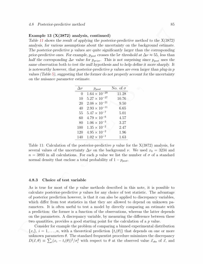
Dra

ftJu

ne13

,20

07


Example 13 (X(3872) analysis, continued)Table 11 shows the result of applying the posterior-predictive method to the X(3872)analysis, for various assumptions about the uncertainty on the background estimate.The posterior-predictive p values are quite significantly larger than the correspondingprior-predictive ones. For example, ppost crosses the 5σ threshold at ∆ν ≈ 55, less thanhalf the corresponding ∆ν value for pprior. This is not surprising since ppost uses thesame observation both to test the null hypothesis and to help define it more sharply. Itis noteworthy however, that posterior-predictive p values are even larger than plug-in pvalues (Table 5), suggesting that the former do not properly account for the uncertaintyon the nuisance parameter estimate.

∆ν ppost No. of σ

0 1.64× 10−29 11.2810 5.27× 10−27 10.7620 2.08× 10−21 9.5040 2.93× 10−11 6.6555 5.47× 10−7 5.0160 4.79× 10−6 4.5780 1.06× 10−3 3.27

100 1.35× 10−2 2.47120 4.95× 10−2 1.96140 1.02× 10−1 1.63

Table 11: Calculation of the posterior-predictive p value for the X(3872) analysis, forseveral values of the uncertainty ∆ν on the background ν. We used x0 = 3234 andn = 3893 in all calculations. For each p value we list the number of σ of a standardnormal density that enclose a total probability of 1− ppost.

4.8.3 Choice of test variable

As is true for most of the p value methods described in this note, it is possible tocalculate posterior-predictive p values for any choice of test statistic. The advantageof posterior prediction however, is that it can also be applied to discrepancy variables,which differ from test statistics in that they are allowed to depend on unknown pa-rameters. It is often useful to test a model by directly comparing an estimate witha prediction: the former is a function of the observations, whereas the latter dependson the parameters. A discrepancy variable, by measuring the difference between thesetwo quantities, provides a good starting point for the calculation of a p value.

Consider for example the problem of comparing a binned experimental distribution{xi}, i = 1, . . . , n, with a theoretical prediction {ti(θ)} that depends on one or moreunknown parameters θ. The standard frequentist procedure minimizes the discrepancyD(~x, θ) ≡

∑i(xi − ti(θ))

2/σ2i with respect to θ at the observed value ~xobs of ~x, and

Dra

ftJu

ne13

,20

07


refers the result to a χ2 distribution to calculate a p value. In contrast, the posterior-predictive approach integrates the joint distribution of ~x and θ given ~xobs,

p(~x, θ | ~xobs) = p(~x | θ,H0) p(θ | ~xobs, H0), (4.8.20)

over all ~x and θ satisfying D(~x, θ) ≥ D(~xobs, θ). Note that this can not be done withinthe prior-predictive approach because, once ~xobs is known, all information about θ iscarried by its posterior, not its prior. Discrepancy variables are also used by the fiducialmethod of section 4.6. In that case however, the discrepancy variables must be pivotalin order to eliminate nuisance parameters.

Reference [73] suggests using a conditional likelihood ratio (CLR) as discrepancyvariable. This is essentially a generalization of the above sum of squared deviationsvariable. If the pdf of the data is p(x |µ, ν), with µ the parameter of interest and ν thenuisance parameter, the CLR is defined as:11

DC(x, ν) ≡supµ∈M0

p(x |µ, ν)supµ 6∈M0

p(x |µ, ν), (4.8.21)

where M0 is the parameter space for µ under the null hypothesis. The term “condi-tional” in CLR refers to a Bayesian conditioning on the value of ν.

For the problem of testing the mean µ of a Poisson signal process in the presenceof a Poisson background process with mean ν, the likelihood is:

L(µ, ν) =(µ+ ν)n

n!e−µ−ν ,

and for testing H0 : µ = 0 versus H1 : µ > 0, the CLR has the form:

− 2 lnDC(n, ν) =

{−2n ln

ν

n− 2 (n− ν) if n > ν,

0 if n ≤ ν.(4.8.22)

The posterior-predictive p value based on this discrepancy variable and an observationn0 is:

ppost,CLR(n0) =∑nrep

∫dν

DC(nrep,ν) ≥ DC(n0,ν)

νnrep e−ν

nrep!p(ν |n0), (4.8.23)

where p(ν |n), the posterior for ν, is given by (4.8.17). In terms of nrep and ν, theregion of summation/integration DC(nrep, ν) ≥ DC(n0, ν) maps out to

(nrep ≥ n0 and ν ≥ 0) or (nrep ≥ 0 and ν ≥ n0).

The summation and integration are then easy to perform, yielding:

ppost,CLR(n0) =

∫ n0

0

dν P (n0, ν) p(ν |n0) +

∫ +∞

n0

dν p(ν |n0). (4.8.24)

11For consistency with our definitions in section 4.3, the CLR defined here is actually the inverse ofthat in reference [73].

Dra

ftJu

ne13

,20

07


Since the incomplete gamma function P (n0, ν) is always less than one, comparison withequation (4.8.19) shows immediately that ppost,CLR(n0) ≥ ppost(n0) in this particularproblem. For the X(3872) example there is hardly any difference between these two pvalues, except at the very highest ∆ν values.

4.8.4 Null distribution of posterior-predictive p values

To check the frequentist uniformity of posterior-predictive p values under the nullhypothesis, the same techniques can be used as before, i.e. starting from equation(4.1.5) and replacing the integration region with ppost(n, x0) ≤ α. Figures 22 and 23show the result for several choices of the true event rate νtrue and the uncertainty ∆ν.In all cases the observed number of events n0 is used as test statistic. At small valuesof α the conservatism is much more dramatic than for prior-predictive p values. Onthe other hand there is some mild liberalism at high values of νtrue and ∆ν, near α = 1(bottom two plots of Figure 22). Using the CLR instead of n0 to compute posterior-predictive p values would enhance their conservative behavior since ppost,CLR ≥ ppost.

It is also possible to check the average uniformity of posterior-predictive p values,by calculating their null distribution over the prior-predictive ensemble:

IPrpp

(ppost(N) ≤ α

)=

∑n

ppost(n)≤α

p(n),

with p(n) the prior-predictive distribution of equation (4.7.4). Since ppost(n) decreasesas n increases, there exists an integer nα such that:

ppost(n) ≤ α ⇔ n ≥ nα.

Therefore:

IPrpp

(ppost(N) ≤ α

)=

+∞∑n=nα

p(n) = pprior(nα),

where the last equality is based on the definition of the prior-predictive p value, equation(4.7.5). Figures 24 and 25 show some examples of this cumulative distribution, whichappears to be conservative for α < 1/2.

The rather extreme conservatism of posterior-predictive p values could easily causeone to keep a null model that is wrong. Reference [57] therefore argues that posterior-predictive p values should be recalibrated with respect to the prior-predictive distri-bution. The authors propose the following corrected posterior-predictive p value whenX = xobs is observed:

pcpost(xobs) ≡ IPr(ppost(X) ≤ ppost(xobs)

), (4.8.25)

where the probability is calculated with respect to the prior-predictive distribution.Because of the latter, one of the main advantages of posterior-predictive p values,namely that they can be used with improper priors, is lost by this recalibration. Theother main advantage, that the more general discrepancy variables can be used insteadof test statistics, remains.

Dra

ftJu

ne13

,20

07


4.8.5 Further comments on prior- versus posterior-predictive p values

We list here some further properties and suggestions for the use of predictive p val-ues: [73]

Comment 1. The prior- and posterior-predictive approaches to the calculation ofp values can be understood in terms of the conditions under which one would re-peat the experiment tomorrow. Under prior-predictive replication, the experimentis repeated assuming that new values will occur for both the data and the parame-ters. Under posterior-predictive replication, the experiment is repeated with the same(unknown) values of the parameters that produced today’s data. Note that, unlikeposterior-predictive replication, prior-predictive replication is undefined for improperprior distributions.

Comment 2. A look at equations (4.7.5) and (4.8.6) suggests an alternative in-terpretation for predictive p values, namely as averages of the classical p value overthe nuisance prior or posterior, respectively. Within this interpretation one can alsocalculate the standard deviation of a predictive p value, as a measure of the spread ofp due to lack of knowledge about the nuisance parameter(s). An upper bound on thestandard deviation is

√p(1− p).

Comment 3. As already emphasized, an important advantage of posterior-predictiveover prior-predictive p values is that the former can be calculated for general discrep-ancy variables as well as for test statistics.

Comment 4. Rather than simply reporting the p value, it may be more informativeto plot the observed value of the test statistic against the appropriate reference distri-bution (i.e. prior-predictive or posterior-predictive). However, this is not possible ifa discrepancy variable D(x, θ) is used instead of a test statistic. In that case, it maybe useful to make a scatter plot of D(xobs, θ) versus D(xrep, θ), where xobs is fixed bythe observation and xrep and θ are drawn from the posterior-predictive distribution.This can be done by Monte Carlo sampling: first draw θ from its posterior distribu-tion, and then draw xrep from its pdf evaluated at the value of θ just drawn. Thefraction of points above the main diagonal in the scatter plot of discrepancies is theposterior-predictive p value.

Comment 5. As the sample size goes to infinity, the posterior distribution will con-centrate at the maximum likelihood estimate of the parameter(s), so that the posterior-predictive distribution will essentially equal the pdf of the data, i.e. the frequentistdistribution commonly used to calculate a p value. In general, the posterior-predictivep value is much more heavily influenced by the likelihood than by the prior, whichgives it a less naturally Bayesian interpretation than the prior-predictive p value.

4.9 Power comparisons and bias

The previous sections illustrated p value calculations with the specific example of aPoisson observation with a Gaussian uncertainty on the mean. The main alternativehypothesis of interest is a Poisson mean that is larger than expected. How likely are

Dra

ftJu

ne13

,20

07

4.10 Summary 89

we to detect such a deviation if it is actually true? This clearly depends on the choiceof test statistic, but also on the method used to eliminate nuisance parameters. Figure26 shows the power of p values, IPr(p ≤ α |H1), for four such methods: supremum,adjusted plug-in, fiducial, and prior-predictive. The test level is set at α = 0.05 andthe power is plotted as a function of the strength of a hypothetical signal superim-posed on the background ν. There is little difference between the supremum and thefiducial method, neither of which is uniformly better than the other. For example, thesupremum method seems to dominate everywhere at small ∆ν values, but not at large∆ν. Prior-predictive power is indistinguishable from fiducial power at small ∆ν, butvisibly smaller at large ∆ν.

The plots also demonstrate that none of the methods is biased, i.e. the probabilityfor rejecting the null hypothesis is always smallest when the latter is true.

4.10 Summary

We have studied seven methods for taking account of systematic uncertainties into pvalue calculations; these are known as the conditioning, supremum, confidence inter-val, bootstrap (plug-in and adjusted plug-in), fiducial, prior-predictive, and posterior-predictive p values. We summarize our findings in this section.

Our first observation, based on the X(3872) example, is that all the p values studiedtend to increase as the uncertainty ∆ν on the rate of the Poisson process increases. Thissatisfies our initial requirement that the probability for rejecting the null hypothesisshould decrease as less is known about that hypothesis.

The X(3872) example has also allowed us to study the asymptotic (i.e. large sample)properties of p values. In this regard, it is quite remarkable that five of the methodsconsidered, namely the supremum, confidence interval, adjusted plug-in, fiducial, andprior-predictive p values give essentially identical results. This gives one confidence inthe robustness of these techniques. It is also understood why the others differ: theposterior-predictive and plug-in p values make double use of the data and are thereforeexcessively conservative; as for the conditioning method, it is not general enough to bedirectly applicable in this example.

The uniformity properties of p values are best studied away from the asymptoticregime, where one tends to expect good behaviour anyway. We found quite a variationin this respect among the methods. For the problem studied, fiducial p values areremarkably near uniformity, and are followed closely by the adjusted plug-in, confidenceinterval, and supremum methods. The adjusted plug-in displays some spotty but minorliberalism, whereas confidence interval and supremum are too generously conservativeat large ∆ν. The prior-predictive p value is even more generous in its conservatism,but perhaps not extremely so. On the other hand, the posterior-predictive and plug-inp values do show disturbingly severe conservatism in some situations and can thereforenot be recommended without additional calibration. The confidence interval methodis by construction “infinitely conservative” for significance levels α lower than β, where1 − β is the confidence level for the nuisance parameter interval. While it may seem

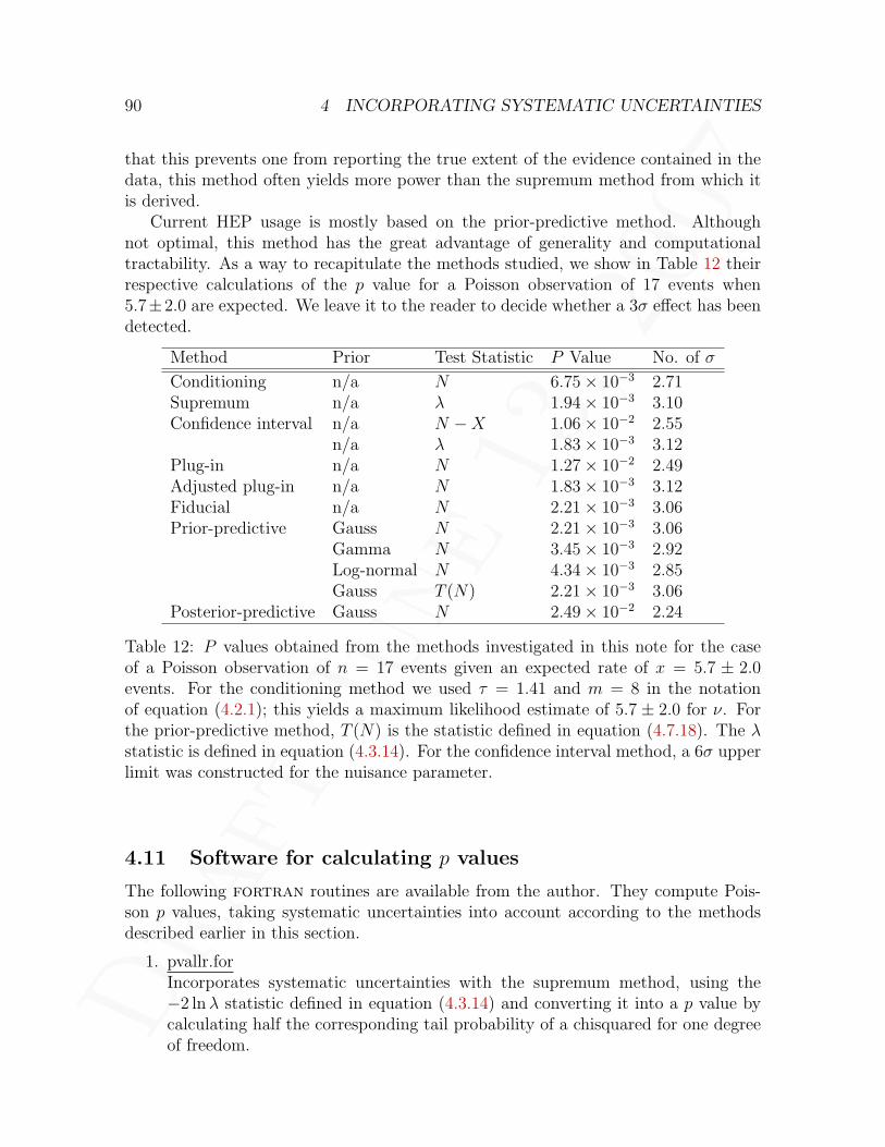
Dra

ftJu

ne13

,20

07


that this prevents one from reporting the true extent of the evidence contained in thedata, this method often yields more power than the supremum method from which itis derived.

Current HEP usage is mostly based on the prior-predictive method. Althoughnot optimal, this method has the great advantage of generality and computationaltractability. As a way to recapitulate the methods studied, we show in Table 12 theirrespective calculations of the p value for a Poisson observation of 17 events when5.7±2.0 are expected. We leave it to the reader to decide whether a 3σ effect has beendetected.

Method Prior Test Statistic P Value No. of σ

Conditioning n/a N 6.75× 10−3 2.71Supremum n/a λ 1.94× 10−3 3.10Confidence interval n/a N −X 1.06× 10−2 2.55

n/a λ 1.83× 10−3 3.12Plug-in n/a N 1.27× 10−2 2.49Adjusted plug-in n/a N 1.83× 10−3 3.12Fiducial n/a N 2.21× 10−3 3.06Prior-predictive Gauss N 2.21× 10−3 3.06

Gamma N 3.45× 10−3 2.92Log-normal N 4.34× 10−3 2.85Gauss T (N) 2.21× 10−3 3.06

Posterior-predictive Gauss N 2.49× 10−2 2.24

Table 12: P values obtained from the methods investigated in this note for the caseof a Poisson observation of n = 17 events given an expected rate of x = 5.7 ± 2.0events. For the conditioning method we used τ = 1.41 and m = 8 in the notationof equation (4.2.1); this yields a maximum likelihood estimate of 5.7 ± 2.0 for ν. Forthe prior-predictive method, T (N) is the statistic defined in equation (4.7.18). The λstatistic is defined in equation (4.3.14). For the confidence interval method, a 6σ upperlimit was constructed for the nuisance parameter.

4.11 Software for calculating p values

The following fortran routines are available from the author. They compute Pois-son p values, taking systematic uncertainties into account according to the methodsdescribed earlier in this section.

1. pvallr.forIncorporates systematic uncertainties with the supremum method, using the−2 lnλ statistic defined in equation (4.3.14) and converting it into a p value bycalculating half the corresponding tail probability of a chisquared for one degreeof freedom.

Dra

ftJu

ne13

,20

07

91

2. pvalci.forComputes confidence interval p values based on equation (4.4.1).

3. pvalpi.forComputes plug-in and adjusted plug-in p values according to equations (4.5.3)and (4.5.7) respectively.

4. pvalgf.forComputes fiducial p values based on equation (4.6.24).

5. pvalpp.forComputes prior-predictive p values according to equation (4.7.8).

6. pvalpo.forComputes posterior-predictive p values according to equation (4.8.19).

All these routines use the cern library.

5 Multiple testing

Multiple testing is not applied very often in particle physics, although there are def-initely several areas where it could prove useful. One such area is the monitoring ofhundreds of thousands of electronic channels at the new LHC experiments. Anotherarea is the search for newly predicted particles in several channels simultaneously. Alsorelevant are the multiple comparisons made by the Particle Data Group [43] to testthe validity of the standard model.

A simple and yet powerful technique to evaluate many tests simultaneously is pro-vided by p value plots.[83] Suppose we are testing n null hypotheses, T0 of which aretrue. Let Np be the number of p values that are greater than or equal to a given p. Wehave then:

E(Np) ≈ T0 (1 − p) (5.0.1)

for p values that are not too small (and therefore likely to come from true null hy-potheses). This suggests a plot of Np versus 1 − p. The left part of the plot will beapproximately linear, with the slope of the “best” straight line through the points be-ing an estimate of the number of true null hypotheses. False hypotheses should yieldsmall p values, which will correspond to points above the line in the right part of theplot.

We illustrate this technique using the results shown in Table 10.4 of the 2004 editionof the Particle Data Group’s review of particle physics.[43] Only results that can beconsidered as more or less independent are of interest; they are reproduced here inTable 13, ordered by increasing discrepancy with predictions. The latter are derivedfrom the global best fit values MZ = 91.1874 ± 0.0021 GeV, MH = 113+56

−40 GeV,Mt = 176.9±4.0 GeV, αs(MZ) = 0.1213±0.0018, and α(MZ)−1 = 127.906±0.019. Asa result, the experimental errors are somewhat correlated with the prediction errors,

Dra

ftJu

ne13

,20

07

92 5 MULTIPLE TESTING

Quantity Measured Value Predicted Value Pull

1. gνeV -0.040 ± 0.015 -0.0397 ± 0.0003 -0.02

2. gνeA -0.507 ± 0.014 -0.5065 ± 0.0001 -0.04

3. QW (T l) -116.6 ± 3.7 -116.81 ± 0.04 0.064. Ac 0.670 ± 0.026 0.6678 ± 0.0005 0.085. MZ (GeV) 91.1876 ± 0.0021 91.1874 ± 0.0021 0.096. Mt (GeV) [CDF] 176.1 ± 7.4 176.9 ± 4.0 -0.117. Rc 0.172 ± 0.003 0.17233 ± 0.00005 -0.11

8. Γ(b→sγ)Γ(b→Xeν)

0.00339 ± 0.00058 0.00323 ± 0.00009 0.28

9. Aµ 0.142 ± 0.015 0.1472 ± 0.0011 -0.3510. As 0.895 ± 0.091 0.9357 ± 0.0001 -0.4511. Ab 0.925 ± 0.020 0.9347 ± 0.0001 -0.49

12. A(0,µ)FB 0.0169 ± 0.0013 0.01626 ± 0.00025 0.49

13. A(0,s)FB 0.0976 ± 0.0114 0.1033 ± 0.0008 -0.50

14. MW (GeV) [LEP 2] 80.412 ± 0.042 80.390 ± 0.018 0.5215. Ae [ang. distr. of τ pol.] 0.1498 ± 0.0049 0.1472 ± 0.0011 0.5316. Rτ 20.764 ± 0.045 20.790 ± 0.018 -0.5817. Mt (GeV) [DØ] 180.1 ± 5.4 176.9 ± 4.0 0.5918. g2

R 0.03076 ± 0.00110 0.03007 ± 0.00003 0.63

19. A(0,e)FB 0.0145 ± 0.0025 0.01626 ± 0.00025 -0.70

20. Aτ [SLD] 0.136 ± 0.015 0.1472 ± 0.0011 -0.75

21. s2`(A

(0,q)FB ) 0.2324 ± 0.0012 0.23149 ± 0.00015 0.76

22. Aτ [total τ pol.] 0.1439 ± 0.0043 0.1472 ± 0.0011 -0.7723. ΓZ (GeV) 2.4952 ± 0.0023 2.4972 ± 0.0012 -0.87

24. A(0,c)FB 0.0706 ± 0.0035 0.0738 ± 0.0006 -0.91

25. Rµ 20.785 ± 0.033 20.751 ± 0.012 1.0326. QW (Cs) -72.69 ± 0.48 -73.19 ± 0.03 1.0427. Re 20.804 ± 0.050 20.750 ± 0.012 1.0828. MW (GeV) [UA2, CDF, DØ] 80.454 ± 0.059 80.390 ± 0.018 1.0829. Rb 0.21638 ± 0.00066 0.21564 ± 0.00014 1.1230. Ae [ALR lept. & pol.Bhabba] 0.1544 ± 0.0060 0.1472 ± 0.0011 1.20

31. A(0,τ)FB 0.0188 ± 0.0017 0.01626 ± 0.00025 1.49

32. 12(gµ − 2− α

π) 4510.64 ± 0.92 4509.13 ± 0.10 1.64

33. ττ (fs) 290.92 ± 0.55 291.83 ± 1.81 -1.6534. σhad (nb) 41.541 ± 0.037 41.472 ± 0.009 1.8635. Ae [ALR hadr.] 0.15138 ± 0.00216 0.1472 ± 0.0011 1.94

36. A(0,b)FB 0.0997 ± 0.0016 0.1032 ± 0.0008 -2.19

37. g2L 0.30005 ± 0.00137 0.30397 ± 0.00023 -2.86

Table 13: Principal Z-pole and other observables, compared with standard modelpredictions and ordered by increasing pull (from Table 10.4 in [43]).

Dra

ftJu

ne13

,20

07

5.1 Combining independent p values 93

which complicates the calculation of pulls. For this example, the pulls only take theexperimental errors into account. Although such a table is useful, it does not providea clear view of the consistency, or lack of it, between measurement and theory. Inparticular, one would like to assess the significance of the most discrepant measurement,a 2.9σ effect. Figure 27 shows the p value plot made from the 37 comparisons inthe table. Each pull zi is converted into a p value pi by assuming a Gaussian errordistribution: pi = 1−erf(|zi|/

√2). The dotted line on the plot is a straight line through

the origin and with a slope of 37, corresponding to all tested hypotheses being true.The points oscillate above and below the line, but nevertheless follow it quite closely.Oscillations in such a plot are due to the natural correlations between order statistics.Additional correlations between the data points will cause further distortions, creatingmore uncertainty in the interpretation of the plot. Overall, the electroweak resultsshown here appear to be in excellent agreement with expectations.

In the remainder of this section we review techniques for combining independentp values and examine a few other procedures that are interesting either because theywork with dependent p values or because of their power properties.

5.1 Combining independent p values

If the individual p values are independent, i.e. they are derived from test statisticswhose joint probability factorizes, then it is fairly straightforward to combine them,although there is no unique way of doing this. The general idea is first to choose a ruleS(p1, p2, p3, . . .) for combining individual p values p1, p2, p3,. . . , and then to constructa combined p value by calculating the tail probability corresponding to the observedvalue of S. Some plausible combination rules are:

1. The product of p1, p2, p3,. . . (Fisher’s rule);

2. The smallest of p1, p2, p3,. . . (Tippett’s rule);

3. The average of p1, p2, p3,. . . ;

4. The largest of p1, p2, p3,. . .

This list is by no means exhaustive. To narrow down the options, there are someproperties of the combined p value that one might consider desirable. [52] For example:

1. If there is strong evidence against the null hypothesis in at least one channel,then the combined p value should reflect that, by being small.

2. If none of the individual p values shows any evidence against the null hypothesis,then the combined p value should not provide such evidence.

3. Combining p values should be associative: the combinations ((p1, p2), p3), ((p1, p3), p2),(p1, (p2, p3)), and (p1, p2, p3) should all give the same result.

Dra

ftJu

ne13

,20

07

94 6 A FURTHER LOOK AT LIKELIHOOD RATIO TESTS

These criteria are of course debatable. Now, it turns out that property 1 eliminatesrules 3 and 4 above. Property 2 is satisfied by all four p values derived from the aboverules. On the other hand, property 3, called evidential consistency by statisticians, issatisfied by none and is therefore not very helpful. This leaves Tippett’s and Fisher’srules as reasonable candidates. Actually, it appears that Fisher’s rule has somewhatmore uniform sensitivity to alternative hypotheses of interest in most problems.

To calculate the combined p value corresponding to Fisher’s rule, there is a neatmathematical trick one can use. First, note that the cumulative distribution of achisquared variate for two degrees of freedom is given by 1−e−x/2. Therefore, if p is anexactly uniform p value, −2 ln p will be distributed as a chisquared with two degrees offreedom. The next step is to remember that chisquared variates are additive: addingk chisquared variates with two degrees of freedom yields a chisquared variate with2k degrees of freedom. Hence the trick: to combine k p values by Fisher’s method,take twice the negative logarithm of their product, and treat it as a chisquared for 2kdegrees of freedom.

For example, to combine two p values p1 and p2, one would refer −2 ln(p1p2) to achisquared distribution for four degrees of freedom. The density of such a chisquaredis xe−x/2/4, and the upper tail probability is (1 + x/2)e−x/2. Setting x = −2 ln(p1p2)in the latter yields [1 − ln(p1p2)]p1p2. The general formula for an arbitrary numberof p values is derived similarly. It becomes a little bit more complicated because thecalculation of the tail probability of a chisquared with an arbitrary number of degreesof freedom involves repeated integrations by parts. The result is:

P

n−1∑j=0

[− ln(P )

]jj!

, (5.1.1)

where P is the product of the n individual p values.The above result is only strictly valid if the individual p values are all derived from

continuous statistics. If one or more p values are discrete, then the formula will give acombined p value that is larger than the correct one, and will therefore be conservative.One can of course always correct for this by running Monte Carlo calculations.

5.2 Other procedures

A review of the abundant literature on combining p values can be found in Refer-ence [26]. The problem of combining p values can be viewed as special case of multipletesting. Some relevant references on the latter are [58, 85, 86, 88, 92].

6 A further look at likelihood ratio tests

As pointed out in section 4.3.1, the likelihood ratio statistic often provides a good start-ing point for testing hypotheses. It is usually easier to compute than the score or Wald

Dra

ftJu

ne13

,20

07

95

statistic, and, in contrast with the latter, is invariant under parameter transforma-tions. A well-known theorem due to Wilks [98] states that the asymptotic distributionof twice the log of the likelihood ratio statistic is chisquared. Wilk’s proof requiresthat the likelihood function admit a second-order Taylor expansion, that the maxi-mum likelihood estimate of the parameter of interest be asymptotically normal, andthat the observations be independent. Interestingly, this theorem can be generalizedin a way that provides a more geometric insight into its conditions. Indeed, Ref. [45]shows that the requirement of asymptotic normality of the MLE can be dropped, andthat if the likelihood contours are fan-shaped, then the log-likelihood ratio statistic isgamma-distributed. More precisely, assume that µ is a p-dimensional parameter andthat the contours of its likelihood can be approximated as:

Sw ≈ µ + anwr S, (6.0.1)

where w is the likelihood ratio value associated with contour Sw, µ is the MLE of µ,an is a sequence converging to zero as the sample size n increases, and S is a surface inRp. Then it can be shown that the log-likelihood ratio is distributed as Gamma(rp).

Example 14Suppose we have a sample of n unstable particles with known decay constant δ andwish to test the hypothesis that their production time τ is properly calibrated:

H0 : τ = τ0

The individual decay times are exponentially distributed:

T ∼ 1

δe−(t−τ)/δ ϑ(t− τ),

where ϑ(t− τ) is the usual step function. The likelihood can be written as:

L(τ) =1

δnen (τ−t)/δ

n∏i=1

ϑ(ti − τ),

with t being the average of the measured decay times. Due to the product of stepfunctions, the MLE of τ is immediately seen to be

τ = min(t1, . . . , tn).

Note that n (τ − τ) is not asymptotically normal. The log-likelihood ratio statistic is:

lnλ =n

δ(τ − τ0) for τ ≥ τ0.

In this simple example the likelihood contours are zero-dimensional:

Sw = {µ :n

δ(τ − τ) = w ≥ 0} = τ +

wδ

nS,

Dra

ftJu

ne13

,20

07


where the “surface” S consists of the single point {µ = −1}. Applying equation (6.0.1)yields an = δ/n and r = 1, so that lnλ is asymptotically distributed as Gamma(1), i.e.2 lnλ is asymptotically distributed as a χ2 with two degrees of freedom. Contrast thiswith the standard, and in this case incorrect result that 2 lnλ should be distributed asa χ2 with one degree of freedom, corresponding to the difference in number of fittedparameters between numerator and denominator of the likelihood ratio.

Unfortunately the above generalization does not cover a number of non-standardsituations, such as when:

1. The null and alternative hypotheses are nonnested, i.e. the null hypothesis can-not be considered as a special case of a more general model represented by thealternative hypothesis;

2. Parameter values in the null hypothesis are on the boundary of the maintainedhypothesis (this is the union of the null and alternative hypotheses);

3. There are nuisance parameters that appear under the alternative hypothesis butare undefined under the null.

The last two of these situations occur quite regularly in high energy physics. We havealready seen an example of the second one in section 4.3.3, where the parameter ofinterest was zero under the null and positive under the alternative. As a result, thedistribution of the likelihood ratio statistic was 1

2χ2

0 + 12χ2

1 instead of simply χ21. In the

present section we concentrate on the third type of problematic situation.

6.1 Testing with weighted least-squares

Section 2.3 described a p value calculation for the observation of a signal peak, theX(3872) resonance, on top of a smooth background spectrum. This calculation dependson the choice of a window in which background and signal events are counted. In orderfor the significance to be unbiased, the window must be chosen before looking at thedata [37], which requires that some information about the location and width of thesignal peak be known beforehand. This was in fact the case for the X(3872), since theBelle collaboration had reported its observation before CDF. [25] If these parametersare unknown, an alternative method is to base the significance calculation on how thefit of the whole spectrum improves when a Gaussian component is added to model theX(3872) signal. For a binned spectrum however, the bin width must still be chosenindependently of the data, which may be difficult without prior information about thesignal width. In this section we consider a binned spectrum and assume that the binwidth was set a priori. We introduce the delta-chisquared statistic and study what canbe said about its distribution under a minimal set of assumptions.

The problem of how a fit behaves under the addition of a signal component canbe formulated as a test of the hypothesis that one or more specific fit parameters arezero. Consider a set of independent measurements yi of a function µ(x) at N different

Dra

ftJu

ne13

,20

07

6.1 Testing with weighted least-squares 97

points xi, and assume that µ(x) depends on s unknown parameters pj, and that yi hasa Gaussian density with mean µi ≡ µ(xi) and known width σi. The likelihood functionis

L(p1, . . . , ps | y1, . . . , yN) =N∏

i=1

e− 1

2

“yi−µi

σi

”2

√2πσi

=e−

12X2

(2π)N/2∏N

i=1 σi

, (6.1.1)

where X2 is the sum of squares:

X2 ≡N∑

i=1

(yi − µi

σi

)2

. (6.1.2)

Suppose now that we are interested in testing the null hypothesis:

H0 : pr+1 = pr+2 = . . . = ps = 0 (6.1.3)

for some r between 0 and s− 1, versus the alternative:

H1 : pi 6= 0 for at least one i ∈ {r + 1, . . . , s}. (6.1.4)

The likelihood ratio statistic for this problem is given by:

λ(y1, . . . , yN) =

sup L(p1, . . . , ps | y1, . . . , yN){p1,...,pr} pr+1=...=ps=0

sup L(p1, . . . , ps | y1, . . . , yN){p1,...,ps}

= e−12δX2

, (6.1.5)

where δX2 is the difference between the sum of squares minimized under H0 and theunrestricted minimized sum of squares:

δX2 = min X2∣∣H0

− minX2. (6.1.6)

A test based on the likelihood ratio statistic can therefore be reformulated as a testbased on the “delta-chisquared” statistic.12 In order to calculate p values, we needthe distribution of δX2 under the null hypothesis. Although the fit presented in Ref-erence [2] involves both linear and non-linear components, the result we will be usingrequires that µ(x) be linear in the parameters pj. Our strategy here is to first gainsome insight by starting from a linear regression model, and then to study the effectof violating various assumptions of this model. We show in appendix B that

If: (a) the function µ(x) is linear in the parameters pj;(b) the yi are mutually independent;(c) the yi are Gaussian with mean µi and width σi;(d) the σi do not depend on the pj;

(6.1.7)

Then: under H0, δX2 has a chisquared distribution with s− r degrees of freedom.

12It is sometimes suggested that an F test be used to determine whether a given parametrizationneeds an additional component. [81] In fact, the F test is the likelihood ratio test for least-squaresfitting problems where the measurements yi all have the same unknown variance σ2. [94] One mustthen estimate σ in addition to the regression coefficients pj . This is clearly not the case of the X(3872)analysis. Of course, one could still use the F test here, but it would not have as much power as theδX2 test, since the latter is equivalent to the likelihood ratio test.

Dra

ftJu

ne13

,20

07


We illustrate this theorem with the problem of fitting a 70-bin histogram that isa random fluctuation of the quadratic polynomial spectrum used to model the back-ground in Figure 1 of Reference [2] and reproduced here in Figure 28a. We wish to testthe null hypothesis that the spectrum is quadratic against the alternative that it has acubic and/or quartic component. To obtain the δX2 distribution we run the followingpseudo-experiment procedure a large number of times:

1. Generate a histogram by Gaussian fluctuations of the null hypothesisspectrum;

2. Fit the generated histogram to a quadratic polynomial by minimizingthe sum of squares (6.1.2); call X2

1 the resulting minimum;

3. Fit the generated histogram to a quartic polynomial, and call X22 the

minimum sum of squares obtained here;

4. Histogram the difference δX2 ≡ X21 −X2

2 .

Note the somewhat unusual choice of Gaussian fluctuations in step 1: this is to satisfycondition (6.1.7c). Figure 29 shows the result of 20,000 runs of the above procedure.The chisquared distributions for the two fits agree fully with expectations: the first fithas 70− 3 = 67 degrees of freedom and the second one 70− 5 = 65. Accordingly, theδX2 distribution coincides nicely with a χ2 density for two degrees of freedom.

6.1.1 Exact and asymptotic pivotality

The reason that the above pseudo-experiment procedure works is that the δX2 statisticis exactly pivotal for this problem, i.e. its distribution is independent of the values ofparameters that are not restricted by H0. Therefore, it does not matter that thefirst step of the procedure does not specify numerical values for the coefficients of thequadratic polynomial under H0: any choice will give the same result.

In practice it is relatively rare to encounter exact pivotality, except in the trivialcase where the null hypothesis is simple and fully specifies all the parameters in theproblem. The distribution of an exact pivot is either known analytically or can beapproximated unambiguously by a Monte Carlo calculation. When a test statisticis not exactly pivotal in finite samples, it may still be so in the large sample limit(asymptotic pivotality). One may then be able to use an asymptotic distribution toapproximate the finite sample distribution of the test statistic. Such a procedure isthen referred to as an asymptotic test.

Another approach to the treatment of asymptotic pivots, which also works for non-pivotal statistics, is the bootstrap. Here one performs a Monte Carlo simulation ofthe distribution of the test statistic under the null hypothesis, substituting consistentestimates for the values of unknown parameters. [7] The resulting p value will notbe exact, since it is obtained from an estimated pdf rather than the true one. How-ever, the difference between the bootstrap p value and the exact one goes to zero asthe sample size increases. Furthermore, it is in principle possible to improve on the

Dra

ftJu

ne13

,20

07

6.1 Testing with weighted least-squares 99

bootstrap p value by a nested double-bootstrap algorithm such as the one describedin section 4.5.1. Of course, in most cases this improvement is not practically achiev-able due to the enormous computational burden it imposes. For test statistics thatare merely asymptotically pivotal, it is generally believed that bootstrap tests performbetter than asymptotic ones. [31, section 4.6]

With respect to exact pivotality, the X(3872) analysis violates conditions (6.1.7a, c,and d): its error structure is not Gaussian but Poisson, and its regression is non-lineardue to the use of a Gaussian to model the ψ(2S) peak on top of the quadratic back-ground spectrum. However, as we illustrate in the next subsections, these violationshave little effect on the accuracy of tests based on the asymptotic pivotality of the δX2

statistic.

6.1.2 Effect of Poisson errors, using Neyman residuals

In a counting experiment without constraint on the total number of counts, histogrambins obey Poisson statistics, so that the σi in equation (6.1.2) must be replaced by√µi. However, when the µi depend on some unknown parameters pj that must be

determined by minimizing X2, this replacement can turn a nice linear problem intoa non-linear one, violating another of the conditions (6.1.7). A possible solution is toreplace σi by

√yi instead. This is sometimes referred to as Neyman’s chisquared [14]:

X2 ≡N∑

i=1

(yi − µi)2

yi

. (6.1.8)

Figure 30 shows the result of running the previously described pseudo-experiment pro-cedure, this time with Poisson fluctuations of the bin contents and using Neyman’schisquared to do the fits. There is good agreement with the expected chisquared dis-tributions.

6.1.3 Effect of Poisson errors, using Pearson residuals

The effect of using Pearson’s chisquared:

X2 ≡N∑

i=1

(yi − µi)2

µi

. (6.1.9)

is shown in Figure 31. These plots are indistinguishable from those obtained for thepurely Gaussian case in Figure 29. This is not a surprise, as it is well known that,asymptotically, Pearson’s chisquared converges faster than Neyman’s to an exact χ2

distribution [41]. According to our discussion in section 2.3.2, Neyman’s chisquaredcorresponds to approximating a chisquared by a Gaussian in each bin, whereas Pear-son’s chisquared corresponds to approximating a Poisson by a Gaussian in each bin.In a regime where these approximations perform poorly, one could consider construct-ing a chisquared from Wilson and Hilferty’s approximation (equation 2.3.12). For theremainder of this study we will simply continue with Pearson’s chisquared.

Dra

ftJu

ne13

,20

07


Since Pearson’s chisquared is based on a Gaussian approximation, it may not bereliable for computing very small p values, even when the sample size is as large as thatof the X(3872) analysis. A plausible estimate of the accuracy of this calculation canbe obtained by some of the methods described in section 2.3. The Poisson probabilityfor an expected background of 3234 events to fluctuate up to 3893 observed events orhigher, corresponds to 11.28σ. With the Gaussian approximation one finds (3893 −3234)/

√3234 = 11.59σ. The difference of 0.3σ should be a good guess of the accuracy

of the fitter-based significance. There are however other sources of bias to consider, aswill be discussed in section 6.2.

6.1.4 Effect of a non-linear null hypothesis

The X(3872) analysis includes a Gaussian to model the ψ(2S) peak, which is part ofthe background. We generated 20,000 pseudo-experiments from a spectrum consistingof this peak on top of the usual quadratic background (see Figure 28b). The first fitis then done to a Gaussian plus a quadratic (six parameters), and the second one toa Gaussian plus a quartic (eight parameters). Figure 32 shows the resulting X2

min andδX2 distributions. They all agree with expectations based on the linear regressionmodel.

6.2 Testing in the presence of nuisance parameters that areundefined under the null

There is one more aspect of the X(3872) analysis that we haven’t tested, namelythe presence of a nonlinear component under the alternative hypothesis: a Gaus-sian distribution to model the X(3872) peak itself. For this we used a set of 20,000pseudo-experiments with a quadratic background spectrum (Figure 28a). Each pseudo-experiment was first fit to a quadratic polynomial (H0) and then again to the sum ofa quadratic polynomial and a Gaussian resonance with a fixed width of 4.3 MeV/c2,the presumed width of the X(3872) state (H1).

Figure 33 shows a large discrepancy between the X2 distribution under H1 and theexpected chisquared distribution. As a result, the δX2 statistic is no longer distributedas χ2

2, a chisquared with two degrees of freedom. In fact, p values calculated using thetheoretical χ2

2 distribution would be seriously underestimated, causing the significanceto be overstated. What happened?

As shown in Appendix D, this problem can be traced back to the fact that whenthe true amplitude of the signal resonance is zero (which is the null hypothesis), thepdf of the data no longer depends on the mean of that resonance. On the other hand,the fit still produces an estimate for that mean. However, this estimate is no longerconsistent, i.e. it does not tend to the true value as the sample size increases. This lossof consistency is responsible for the breakdown of linearity in the asymptotic limit. Inthe literature, the resonance mean is referred to as a nuisance parameter “that is onlypresent under the alternative,” or “that is undefined under the null.”

Dra

ftJu

ne13

,20

07

6.2 Testing in the presence of nuisance parameters that are undefined under the null101

In the next several sections, we discuss some valid methods for estimating thesignificance in this case.

6.2.1 Lack-of-fit test

The first method is based on the observation that the distribution of the χ2 goodness-of-fit statistic for the null hypothesis fit is still adequately described by its asymptoticlimit (Figure 33, top left). Thus one could still do a goodness-of-fit test on the observedspectrum. The disadvantage of this approach is that it is sensitive to a wide rangeof alternatives and much less powerful than the δX2 test at detecting the specificalternative we are interested in. The p value obtained from a goodness-of-fit test istherefore likely to underestimate the true significance of the observation.

A possible improvement on this method is described in Reference [49].

6.2.2 Finite-sample bootstrap test

A brute-force approach to the problem is to generate a large number of pseudo-experiments from the null hypothesis model for the data, and to calculate the δX2

test statistic for each pseudo-experiment. The resulting distribution of δX2 can thenbe used to evaluate the significance of the observed δX2 value. If the backgroundshape under the X(3872) signal was fully known, the δX2 statistic would be exactlypivotal. Although its distribution would not be known in analytical form, it could stillbe determined unambiguously by this Monte Carlo calculation. As it stands however,the shape of the X(3872) background is not known and must be estimated from data.One must therefore use the bootstrap method.

A major difficulty with this method is the calculation of the δX2 statistic for eachpseudo-experiment, which requires two fits, one under the null hypothesis and thesecond under the alternative. The second fit can be particularly difficult because itrequires that one find the largest signal-like fluctuation among many local fluctuationsin a spectrum generated from the background-only hypothesis. In this situation, mostfitters (including CERN’s minuit) will only find the local maximum closest to thestarting point of the fit. The only way to locate the global maximum is to repeat thefit at several points between the spectrum boundaries. Further details on this methodare provided in Appendix D.

A possible saving of CPU time can be obtained as follows. Let δX2obs be the

δX2 value observed in the actual data. Any pseudo-experiment that is sufficientlybackground-like to satisfy

X2min|H0 < δX2

obs, (6.2.1)

also satisfies the following inequality on its δX2:

δX2 = X2min|H0 − X2

min < δX2obs − X2

min < δX2obs,

and therefore does not contribute to the numerator of the bootstrap p value. Notethat we can figure this out without having to calculate the fit chisquared under the

Dra

ftJu

ne13

,20

07


alternative hypothesis, hence the saving in CPU time. How substantial this saving isdepends on the difference in number of degrees of freedom between X2

min|H0 and δX2.If it is large, inequality (6.2.1) is unlikely to obtain very often, and savings will beminimal.

It should be clear by now that the bootstrap method can be computationally veryintensive and won’t provide answers in the region of the X(3872), where δX2

obs is oforder 100.

6.2.3 Asymptotic bootstrap test

A considerable simplification is achieved by working directly with the asymptotic ex-pression for the δX2 statistic, for a fixed value of the mean θ of the X(3872) resonance.This expression is derived in Appendix B:

δX2(θ) = [q4(θ)]2 , (6.2.2)

where q4(θ) is a linear combination of Gaussian variates that represent asymptoticapproximations to the bin contents yi. Furthermore, q4(θ) is directly proportional tothe fitted amplitude of the X(3872) resonance at location θ. The great simplificationof this approach is that all the fit parameters have been eliminated, except for θ.

What we have done so far is to treat θ as a fit parameter, adjusting it to minimizeX2 under the alternative hypothesis, which assumes that the X(3872) amplitude ispositive. This is equivalent to maximizing δX2(θ) with respect to θ, effectively workingwith the one-sided statistic:

δX2sup(1s) =

[max

(sup

L≤θ≤Uq4(θ) , 0

)]2

, (6.2.3)

where L and U denote the boundaries of the fitted spectrum. On the other hand, ifthere was some physics reason to allow negative X(3872) amplitudes, one could workwith the two-sided statistic:

δX2sup(2s) = sup

L≤θ≤U[q4(θ)]

2 . (6.2.4)

To illustrate the calculation of δX2sup, we show in Figure 34(a) a random histogram of

yi generated from a quadratic spectrum, and in Figure 34(b) the corresponding q4(θ)function. As expected, the variation of q4(θ) with θ tends to track fluctuations of theyi above or below their expectations. It is clear that a local minimizer such as minuitcan not efficiently find the global maximum in equation (6.2.3) or (6.2.4). Fortunately,since this is a one-dimensional, bounded problem, one can do a simple grid search bystepping through 1001 equidistant points between L and U and using the largest ofthe function values at these points. The result of this grid search is compared with thefinite-sample bootstrap method in Figure 35. There is good agreement between thetwo methods for the X(3872) analysis.

Dra

ftJu

ne13

,20

07

6.2 Testing in the presence of nuisance parameters that are undefined under the null103

6.2.4 Analytical upper bounds

Reference [4] shows that hypothesis tests based on the supremum statistics of equations(6.2.3) and (6.2.4) are optimal in a certain sense, whereas References [32, 33] provideupper bounds on the null-hypothesis tail probabilities of these statistics. One suchupper bound, applicable to the X(3872) analysis, is:

IPr{δX2

sup(1s) > u∣∣∣H0

}≤ 1

2

[∫ +∞

u

e−x/2

√2π x

dx +K

π

∫ +∞

u

e−x/2

2dx

]

=1

2

[1− erf

(√u/2)]

+K

2πe−u/2. (6.2.5)

The right-hand side is a linear combination of tail probabilities for chisquared distri-butions with one and two degrees of freedom. In the second term, K is a constant thatdepends on the range [L,U ] of the Gaussian mean θ:

K =

∫ U

L

√Var

(dq4dθ

)dθ. (6.2.6)

An expression for the variance appearing in the integrand is provided by equation(B.0.40) in Appendix B. The integrand of equation (6.2.6) is shown as a function ofthe integration variable θ in Figure 36(a). Integrating numerically from 3.65 to 4.00yields K ≈ 60.98. The resulting upper bound of equation (6.2.5) is compared with afinite-sample bootstrap calculation in Figure 36(b). For δX2

sup(1s) > 6, the upper boundappears to turn into an excellent approximation of the bootstrap result, instilling someconfidence in its applicability to the X(3872) analysis.

For the actual X(3872) analysis it is probably sensible to exclude the vicinity of theψ(2S) peak from the range of plausible values for θ. Setting this range to [3.75 , 4.00]GeV/c2, we find K ≈ 43.25. For Figure 2 in reference [2] the statistic δX2

sup(1s) is

approximately 107.6. Using equation (6.2.5), this corresponds to a (one-sided) tailprobability of 2.986 × 10−23, or 9.93σ. Had we used chisquared tables for one ortwo degrees of freedom instead, we would have obtained significances of 10.44σ or10.19σ, respectively. For this particular example, the difference is of the same orderas the accuracy of the Gaussian approximation to the Poisson derived in section 6.1.3.Note however that the Gaussian approximation to the Poisson improves as the samplesize increases. Take for example two 10σ observations over predicted backgrounds ofrespectively 4, 000 and 40, 000 events. In the first case, the Gaussian approximation tothe tail probability is too low by a factor of about 7.2. In the second case, with tentimes more statistics, the Gaussian approximation underestimates the correct resultby a factor of only 1.2, a clear improvement. On the other hand, no such improvementoccurs for the effect of nuisance parameters that are present under the alternativehypothesis only. Consider equation (6.2.5), which applies to situations with one degreeof freedom and one nuisance parameter (in the X(3872) analysis, the amplitude and

Dra

ftJu

ne13

,20

07


mean of the resonance, respectively). The ratio of the correct tail probability to thatof half a chisquared for two degrees of freedom is K/π at large values of u13, and Kdoes not go to zero for large sample sizes. For the X(3872) analysis, K/π is about 14.

6.2.5 Other test statistics

The approach discussed in the previous subsection consists in treating the locationparameter θ of the X(3872) resonance as a nuisance parameter which one must try to“eliminate” in some way. The δX2

sup(1s) and δX2sup(2s) statistics perform this elimination

by calculating a supremum. Other possibilities would be to average or integrate overθ. This is investigated in Reference [3], which introduces the following statistics:

AveLR2s =

∫ U

L

dθ w(θ) δX2(θ), (6.2.7)

ExpLR2s = ln

∫ U

L

dθ w(θ) exp[ 1

2δX2(θ)

], (6.2.8)

where w(θ) is a weight function that depends on the problem at hand and should bechosen to optimize power against alternatives of interest. These are two-sided statistics.One-sided versions can be defined with the help of the step function ϑ(·):

AveLR1s =

∫ U

L

dθ w(θ) ϑ[q4(θ)

]δX2(θ), (6.2.9)

ExpLR1s = ln

∫ U

L

dθ w(θ) ϑ[q4(θ)

]exp[ 1

2δX2(θ)

]. (6.2.10)

The distribution of these statistics underH0 orH1 can be computed with a finite-sampleor asymptotic bootstrap method. As was the case with the supremum statistics (6.2.3)and (6.2.4), the asymptotic bootstrap is by far the easier method to program.

An obvious question at this point is which of the three statistics, ExpLR, AveLR,and SupLR (≡ δX2

sup), one should use. One way to answer is by studying the powerof the corresponding tests in a problem such as the X(3872) analysis. This is shownin Figures 37 and 38. The power functions of ExpLR and SupLR are essentially in-distinguishable, whereas that of AveLR is intermediate between SupLR and a simplegoodness-of-fit test. All four power functions are of course lower than that of a likeli-hood ratio test based on exact knowledge of the X(3872) location.

6.2.6 Other methods

The problem of testing when nuisance parameters are present only under the alterna-tive has been extensively studied in the statistical literature. Some examples follow.

13To understand why we are comparing the correct tail probability to half a chisquared for twodegrees of freedom, remember that the statistic δX2

sup(1s) only takes into account positive amplitudesof the X(3872) signal.

Dra

ftJu

ne13

,20

07

6.3 Summary of δX2 study 105

Reference [95] uses the theory of Euler characteristics to generalize formula (6.2.5) tomore than one nuisance parameter. In [76], a score test is proposed, and an asymp-totic approximation to its null distribution is derived using Hotelling’s volume-of-tubeformula. Reference [62] suggests a parameter transformation to remove the nuisanceparameter that is present only under the alternative and replace it by an additional re-striction underH0. This changes the nature of the difficulty, making it sometimes easierto solve, but not always. Finally, Reference [23] proposes an interesting directed-graphmethod to break down an irregular testing problem into regular components.

6.3 Summary of δX2 study

A careless evaluation of the significance of the X(3872) observation would consist inreferring the observed δX2 value to a chisquared distribution for two degrees of freedom,corresponding to the amplitude and mean of the signal resonance. One could arguethat the corrections due to the use of a Gaussian approximation to Poisson statisticson the one hand, and to the presence of a nuisance parameter under the alternativehypothesis only on the other, are very small compared to the estimated significance.It should be noted though, that both corrections reduce the significance.

In general one will always need to be careful about the effects just discussed, and inparticular about the asymptotically irreducible effect of nuisance parameters that arenot identified under the null hypothesis. This often occurs with nonlinear models suchas those used to describe Gaussian resonances. If the mean and width of the resonanceare known, there is no problem since the amplitude is a linear parameter. If eitherthe mean or the width, or both, are unknown, then the correct distribution of thetest statistic must be determined by one of the special methods discussed previously.Unfortunately most of these methods become very quickly intractable as the numberof nuisance parameters unidentified under H0 increases above 1.

6.4 A naıve formula

The Belle Collaboration [25] based the significance calculation of their own X(3872)observation on the following formula:

“Number of sigma” =

√−2 ln

(L0

Lmax

), (6.4.1)

where L0 (Lmax) is the value of the likelihood maximized without (with) a signal com-ponent in the fitted model. The right-hand side is essentially a transformed likelihoodratio. If the signal component of the model only has one free parameter, and if all theother assumptions of the relevant theorem are satisfied, then the distribution of twicethe negative log-likelihood ratio is that of a chisquared with one degree of freedom.Taking the square root then yields the absolute value of a Gaussian variate with zeromean and unit variance, hence the equality with the left-hand side.

Dra

ftJu

ne13

,20

07

106 7 EFFECT OF TESTING ON SUBSEQUENT INFERENCE

In the simplest version of the X(3872) analysis however, the signal resonance has twofree parameters, amplitude and mean, and estimators for the mean are not consistentwhen the true value of the amplitude is zero. The theorem therefore does not apply.Even if it did, the fact that there are two fit parameters for the signal makes equation(6.4.1) only approximately valid. To illustrate this last point, we plot in figure 39chisquared tail probabilities for one, two, three, and four degrees of freedom. On thatgraph, a given tail probability p is expressed as the number of standard deviations ofa Gaussian density that enclose an area 1 − p around the mean. For example, whatappears to be a 5σ effect with the above formula is only 4.6σ, 4.3σ, and 4.1σ if theactual number of degrees of freedom is 2, 3, and 4, respectively. However, the relativeaccuracy of the approximation does increase with the observed value of the chisquaredvariate.

7 Effect of testing on subsequent inference

Searches for new physics are typically done in one of two ways. If a theory predicts theexistence of a new particle, evidence for the latter can be obtained by testing whetherits production rate is zero or positive. However, new phenomena can also manifestthemselves by an extra contribution to a known, measurable quantity; one can thentest whether that quantity equals its standard model value or exhibits a deviation inthe direction predicted by the new physics. In both cases it is possible to identify a(usually continuous) parameter µ, such that one is interested in testing, say, H0 : µ = 0versus H1 : µ > 0. Furthermore, it is often useful to supplement the test result with arange of µ values that are favored or disfavored by the data. A common procedure forsolving this problem is the following:

(1) Test the null hypothesis H0, say at the α0 = 5.7× 10−7 significance level (5σ);

(2a) If H0 is not rejected, report an α1 = 95% confidence level upper limit on µ;

(2b) If H0 is rejected, report an α2 = 68% confidence level two-sided interval for µ.

Notice that this procedure involves three independent confidence levels, α0, α1, and α2.With the choice of α0 one seeks to establish a strong standard of discovery, as discussedin section 2.2. When no discovery can be claimed, one is forced to keep working withthe null hypothesis µ = 0. To insist nevertheless on calculating an interval for µ wouldseem superfluous, if not logically inconsistent. However, the failure to reject H0 doesnot mean that the latter is true, since the experimental apparatus has finite sensitivityand the data could exhibit a background-like fluctuation when signal is present. Henceit is often useful to determine a range of values of µ that the experimental conditions,together with the observations, do not really permit to “distinguish” from the nullvalue of µ. By definition this range includes the null value itself, which implies thatit must take the form of an upper or lower limit if the initial test is one-sided. Sinceparameter values beyond the limit are considered “distinguishable” from the null value,

Dra

ftJu

ne13

,20

07

107

and therefore excluded by the data, it is wise to choose a reasonably high confidencelevel α1 for the limit. A popular choice is 95%, corresponding approximately to 2σin the tail of a Gaussian distribution. We emphasize here that the reported limitshould not just be an expected limit, but should include information contributed bythe observed data. Finally, if a discovery is claimed, it is important to quantify themagnitude of µ that gave rise to the observation. Since the test indicates that µ mayindeed be different from zero, a two-sided interval is appropriate. Furthermore, we aremore interested in the values of µ inside the interval than in those outside, so thatinterval should not be too large. This leads to the standard choice α2 = 68%.

Although the above procedure may seem to have rather sensible inferential goals, itis a classic example of “flip-flopping,” in which a user decides what type of interval toreport based on the data. [46] This can be seen most directly from a plot of the coveragethat would result from such a procedure. Suppose that µ is the mean, assumed tobe positive or zero, of a Gaussian pdf with known width σ, and we have made oneobservation x of µ. The critical region for rejecting the hypothesis that µ = 0 has theform x ≥ nσ, with n being typically between 3 and 5. The overall coverage C(µ) isthen the sum of two components, one associated with the upper limit reported whenx < nσ and the other with the two-sided interval reported when x ≥ nσ (we assumehere that the two-sided interval is constructed with a central ordering rule):

C(µ) =[α1 − β(µ, n)

]+

+ min

{α2,

1

2

[α2 + 2β(µ, n)− 1

]+

}, (7.0.2)

where [x]+ equals x when the latter is positive and zero otherwise, and β(µ, n) is thepower function of the test:

β(µ, n) =

∫ +∞

nσ

dxe−1

2

„x−µ

σ

«2

√2π σ

=1

2

[1 + erf

(µ− nσ√2σ

)]. (7.0.3)

The function C(µ) is plotted in Figure 40 for n = 5 and several values of α1 and α2.The standard choice of α1, α2 is shown in plot (d). It is clear that the question ofcorrect coverage is ill-posed when α1 6= α2. On the other hand, when α1 = α2 thereis a region of parameter values for which the procedure undercovers. Note also thatundercoverage almost always occurs for µ = 0, since C(0) = [α1 − β(0, n)]+ < α1

whenever n ≥√

2 erf−1(α2). However, this effect is negligible for large values of n.Perhaps a more relevant way to investigate the coverage of our search procedure is

to condition on an appropriate subset of experimental results. In this approach, thecoverage of the upper limit is calculated within the subset of experiments that fail toreject the null hypothesis, and the coverage of the two-sided interval is referred to thesubset of experiments that claim a discovery. For the example of a Gaussian pdf withpositive mean, the conditional coverage of the upper limit is:

C1s(µ) =1

1 − β(µ, n)

[α1 − β(µ, n)

]+, (7.0.4)

Dra

ftJu

ne13

,20

07


and that of the two-sided interval is:

C2s(µ) =1

β(µ, n)min

{α2,

1

2

[α2 + 2β(µ, n)− 1

]+

}. (7.0.5)

These results are illustrated in Figure 41 for the case α1 = 0.95 and α2 = 0.68. Thecoverage of the upper limit is optimal for small values of µ, where one expects mostobservations to fall below the discovery threshold. The opposite is true for the two-sidedinterval, which has good coverage at large values of µ. The coverage of each constructionfails dramatically in the region where the coverage of the other construction is optimal.

To overcome the lack of coverage of the above procedure, Ref. [46] advocates theconstruction of intervals based on the likelihood ratio ordering rule. Such intervalshave exact coverage (at least in the continuous case) and evolve naturally from one-sided to two-sided as the estimate of µ moves away from its null value. Unfortunatelythere is only one degree of freedom in the choice of confidence levels: one has to takeα0 = α1 = α2. As argued above, this is incompatible with common desiderata andleads either to intervals that are too wide or test levels that are too low. An alternativemethod is to calculate conditional confidence intervals. We discuss this option in thenext section.

7.1 Conditional confidence intervals

Reference [72] elegantly summarizes the principle that should be followed when esti-mation is performed after testing:

Most commonly, a test of hypothesis is a partition of the sample space into a criticalregion and its complement. When estimation is performed only if the test datum is ina particular element of that partition, that element is the sample space for estimationpurposes.

Since the second step of our search procedure is to calculate an upper limit or two-sided interval depending on the test result, we apply the above principle separately toeach case. When no discovery is claimed, this means that the upper limit should beconstructed from the conditional pdf of the data, given that the observation fell outsidethe critical region. We illustrate this again with the example of a Gaussian pdf withknown width σ and positive mean µ. Having made one observation x, we wish to testH0 : µ = 0 versus H1 : µ > 0. The critical region is x ≥ nσ. The conditional densityof x, given x < nσ, is then:

f1(x) =1

1− β(µ, n)

e−1

2

„x−µ

σ

«2

√2π σ

θ(nσ − x), (7.1.1)

where θ(·) is the usual step function and β(µ, n) is the power function of the test,given by equation (7.0.3). We use f1(x) in the standard Neyman construction of upperlimits. This yields an implicit equation for the α1 confidence level upper limit uα1 :

uα1 = x +√

2σ erf−1[1 − 2

(1− α1

) (1− β(uα1 , n)

)], (7.1.2)

Dra

ftJu

ne13

,20

07

7.1 Conditional confidence intervals 109

which can easily be solved by numerical methods. Note that in the limit of large nthe search procedure always fails to reject, its power goes to zero, and one recoversthe usual formula for upper limits. This formula is also recovered when x decreases,since this causes uα1 , and therefore β(uα1 , n), to decrease. The Neyman construction ofthe conditional upper limit is shown in Figure 42, to the left of the dotted line (whichrepresents the 5σ discovery threshold). As the 5σ boundary is approached, the upperlimit diverges. This is the consequence of requiring coverage for large values of µ andreflects the possibility that these fluctuate down, below the discovery threshold.

To construct a conditional two-sided interval on µ, given x ≥ nσ, we start from theappropriate conditional pdf when a discovery is claimed:

f2(x) =1

β(µ, n)

e−1

2

„x−µ

σ

«2

√2π σ

θ(x− nσ). (7.1.3)

Applying the Neyman construction for a central two-sided interval [aα2 , bα2 ] with con-fidence level α2 yields the following implicit equations:

aα2 = x −√

2σ erf−1[1 − (1− α2) β(aα2 , n)

], (7.1.4a)

bα2 = x −√

2σ erf−1[1 − (1 + α2) β(bα2 , n)

]. (7.1.4b)

For large power, β → 1, or large x, these equations yield the standard formulae forunconditional central confidence intervals. The Neyman construction of the conditionalinterval is illustrated in Figure 42, to the right of the dotted 5σ boundary. As thatboundary is approached from the right, the two-sided interval turns into an upper limit.This takes into account the possibility that fluctuations from small values of µ can leadto discovery.

Since the conditional upper limit (7.1.2) and two-sided interval (7.1.4) were obtainedwith Neyman’s construction, they cover exactly within their respective element of thepartition of sample space induced by the hypothesis test. It is also interesting tolook at the overall coverage of the conditional procedure; in other words, what is theprobability that µ will be contained in whatever interval is reported, regardless ofwhether discovery is claimed or not? It is easy to see that the answer must be:

C?(µ) = α1

[1 − β(µ, n)

]+ α2 β(µ, n), (7.1.5)

since β(µ, n) is the probability of claiming discovery when µ is the true value. Thisresult should be compared with equation (7.0.2). In particular, if α1 = α2 ≡ α, weobtain C?(µ) = α, in contrast with C(µ), which undercovers for some values of µ (seeplots (a) and (b) in Figure 40).

An occasional objection to the unconditional upper limit construction for the Gaus-sian problem with positive mean is that for small x it yields a negative upper limitand hence an empty interval. As can be seen from Figure 42, the same effect occurs

Dra

ftJu

ne13

,20

07


for the conditional construction. Whether or not this is a problem depends on one’spoint of view. Small x values (i.e. large negative ones) are evidence against both thenull and alternative hypotheses, and may require a revision of the overall model forthe data. Alternatively, one might consider relaxing the confidence level of the upperlimit, for instance changing it from 95% to 99% or even higher. Another proposal[46] is to replace the upper limit ordering rule by a likelihood ratio one. The resultof this replacement is shown in Figure 43. Although the upper limit is now nowherenegative, it turns into a two-sided interval well before the discovery threshold, a directconsequence of maintaining exact coverage near µ = 0. Unfortunately, as discussed atthe beginning of section 7, this behavior is incompatible with one’s inferential goalswhen no discovery can be claimed.

7.2 Further considerations on the effect of testing

In the previous section we adopted a frequentist approach to hypothesis testing and in-terval construction. It may seem that the considerations that led to the requirement ofconditional estimation would be irrelevant in a Bayesian approach, which by definitionconditions fully on the observations. This reasoning is not always applicable however.The type of search procedure we discussed involves a parameter of interest µ aboutwhich hardly anything is known a priori. A Bayesian analysis would therefore typicallybe based on a noninformative prior for µ, and the performance of the method wouldhave to be judged, inter alia, by its frequentist properties. Thus one would again beforced to introduce an appropriate reference ensemble of experiments.

A fundamental characteristic of Bayesian inference is that experimental outcomesnot actually observed are irrelevant. The prior probability distribution is simply up-dated on the basis of the information received. Nevertheless, subtleties may arise intesting procedures where the outcome of the test determines what data are reported.In those cases it may be necessary to model the data reporting process along with thedata generating process in the construction of the likelihood function. How and whenthis needs to be done is discussed in Reference [35].

In contrast with the example discussed in the previous section, the effect of testingon inference may become relevant at a much earlier stage of the analysis, for instancewhen modeling the shape of a background spectrum. This is often done by least-squares regression, without knowing a priori the type and number of regressors thatare present in the true model. To resolve this problem, some kind of stepwise procedureis used, whereby higher-order regressors are added until an acceptable goodness-of-fitis obtained. The regression coefficients themselves are subsequently estimated as if themodel was fully known a priori, without taking into account the uncertainty due to themodel selection step. This leads to bias in point estimates and undercoverage in intervalestimates of these coefficients. As explained in Reference [63], asymptotic approxima-tions are usually not reliable in this case, and cannot even be helped by bootstrapmethods. The basic problem is that even if one has a consistent estimate of a given re-gression coefficient, that estimate does not converge uniformly to its asymptotic limit,

Dra

ftJu

ne13

,20

07

ACKNOWLEDGEMENTS 111

and its properties depend strongly on the unknown true values of other coefficients.This is still a topic of ongoing research within the statistical community. [56]

Acknowledgements

This report benefitted from discussions with, and comments from members of the CDFstatistics committee and participants at the PhyStat workshops.

Dra

ftJu

ne13

,20

07

112 A LAPLACE APPROXIMATIONS

Appendix

A Laplace approximations

In this appendix we derive equation (4.7.23) in section 4.7.4, from which the Laplaceapproximation to the prior-predictive p value is obtained.

The Laplace approximation applies to integrals of the form∫ b

a

g(x) et h(x) dx (A.0.1)

where:

• g and h are twice continuously differentiable in ]a, b[;

•∫ b

a|g(x)| exp(h(x)) dx exists;

• h reaches a single maximum in c ∈ ]a, b[, and c is the only point where h′ changessign;

• g(c) 6= 0.

Then, for t in the vicinity of +∞ (see any advanced calculus book, for example [39,pg. 125]): ∫ b

a

g(x) et h(x) dx ∼

√2π

−t h′′(c)g(c) et h(c). (A.0.2)

We wish to apply this theorem to the following integral:

I =

∫ +∞

0

νn e−ν

n!K e−

12(

ν−ν0∆ν )

2

dν, (A.0.3)

where

K =

{√2π∆ν

1

2

[1 + erf

(ν0√2∆ν

)]}−1

. (A.0.4)

To make the theorem applicable, we identify the parameter t in (A.0.2) with 1/∆ν2.Our approximation will therefore be valid in the limit ∆ν → 0. A naive application ofthe theorem yields:

I ∼ νn0 e

−ν0

n!, (A.0.5)

which is not very useful. To improve on this, note that by reexpressing K as a Gaussianintegral, I can be written as a ratio of integrals:

I =

∫∞0e−

12(

ν−ν0∆ν )

2νn e−ν

n!dν∫∞

0e−

12(

ν−ν0∆ν )

2

dν. (A.0.6)

Dra

ftJu

ne13

,20

07

113

The next idea [96] is to apply the Laplace method separately to the entirety of thenumerator and to the denominator of equation (A.0.6), so that common error termswill cancel in the ratio. Accordingly, for the numerator we identify the function h ofthe theorem with:

hnum.(ν) = −1

2(ν − ν0)

2 − ∆ν2 (ν − n ln ν + lnn!). (A.0.7)

Although this function does depend on t ≡ 1/∆ν2, this dependence does not havea detrimental effect on the final result as long as ∆ν and n are not too large. Thefunction hnum. reaches its maximum at:

νn =ν0 −∆ν2

2+

√(ν0 −∆ν2

2

)2

+ n∆ν2, (A.0.8)

and its second derivative at the maximum is:

h′′num.(νn) = −1 − n

(∆ν

νn

)2

. (A.0.9)

For the denominator, we have:

hden.(ν) = −1

2(ν − ν0)

2. (A.0.10)

This function reaches its maximum at ν0, and h′′den.(ν0) = −1. We are now ready tocompute the improved Laplace approximation to I:

I ∼√−2π/h′′num.(νn) ehnum.(νn)/∆ν2√−2π/h′′den.(ν0) ehden.(ν0)/∆ν2

∼ e−12(

νn−ν0∆ν )

2√(νn)2 + n∆ν2

(νn)n+1 e−νn

n!. (A.0.11)

This is equation (4.7.23), as promised.

B Asymptotic distribution of the δX2 statistic

Section 6 relies on a result about the asymptotic distribution of the δX2 statistic. Werestate and prove this result here. A byproduct of the proof is a closed expression forthe asymptotic limit of the likelihood ratio statistic, which is used in the example thatfollows the proof.

Theorem:

Consider N observations (xi, yi), where the xi are known, fixed constants and

Dra

ftJu

ne13

,20

07

114 B ASYMPTOTIC DISTRIBUTION OF THE δX2 STATISTIC

the yi are independent measurements that are normally distributed with meansµi ≡ µ(xi) and widths σi. Assume that µ(x) depends linearly on s unknownparameters pj:

µ(x) =s∑

j=1

pj fj(x), (B.0.12)

and that the σi are known constants (independent of x and pj). For some rbetween 0 and s− 1 consider testing

H0 : pr+1 = pr+2 = . . . = ps = 0 (B.0.13)

versusH1 : pj 6= 0 for at least one j ∈ [r + 1, s], (B.0.14)

using the delta-chisquared:

δX2 ≡ minp1,..., pr

X2∣∣H0

− minp1,..., ps

X2, (B.0.15)

where:

X2 ≡N∑

i=1

(yi − µi

σi

)2

. (B.0.16)

Then, the distribution of δX2 under H0 is that of a chisquared with s− r degreesof freedom.

Proof:

Start by defining a scalar product for arbitrary functions f1, f2 with support {x1, . . . , xN}:

〈f1|f2〉 ≡N∑

i=1

f1(xi) f2(xi)

σ2i

, (B.0.17)

and orthonormalize the functions fj(x) used in the definition of µ(x). This can be doneby the standard recursive Gram-Schmidt algorithm:

gi(x) =

f1(x)√〈f1|f1〉

for i = 1,

fi(x) −∑i−1

j=1 〈gj|fi〉 gj(x)√〈fi|fi〉 −

∑i−1j=1 〈gj|fi〉2

for i = 2, 3, . . .

(B.0.18)

Since the gi(x) are linear combinations of the fi(x), we can rewrite µ(x) as:

µ(x) =s∑

j=1

pj fj(x) =s∑

j=1

qj gj(x), (B.0.19)

Dra

ftJu

ne13

,20

07

115

from which expressions for the coefficients qj as linear combinations of the pj canbe derived. According to equation (B.0.18), each gj(x) only depends on fk(x) withk ≤ j. Therefore each pk only depends on qj with j ≥ k, so that the null hypothesis isequivalent to:

H0 : qr+1 = qr+2 = . . . = qs = 0. (B.0.20)

Using the scalar product notation (B.0.17), and expanding µ(x) in terms of the gj, theX2 of equation (B.0.16) can be written as:

X2 = 〈y | y〉 + 〈µ |µ〉 − 2 〈y |µ〉 = 〈y | y〉 +s∑

j=1

q 2j − 2

s∑j=1

qj 〈y | gj〉, (B.0.21)

where we used the orthonormality of the gj to expand 〈µ |µ〉. To minimize this X2 weset ∂X2/∂qj = 0, obtaining:

qj = 〈y | gj〉 =N∑

i=1

yi gj(xi)

σ2i

. (B.0.22)

Substituting this solution in the expression for X2 yields:

X2min =

N∑i=1

(yi

σi

)2

−s∑

j=1

q 2j . (B.0.23)

Under H0 we only need estimators for q1, . . . , qr, since the rest are zero, by (B.0.20).Therefore:

X2min

∣∣H0

=N∑

i=1

(yi

σi

)2

−r∑

j=1

q 2j , (B.0.24)

and:

δX2 = X2min

∣∣H0

− X2min =

s∑j=r+1

q 2j . (B.0.25)

Finally, note that, by orthonormality of the gj(x), the qj have unit variances:

Var(qj) = Var

[N∑

i=1

yigj(xi)

σ2i

]=

N∑i=1

[gj(xi)

σ2i

]2

Var(yi)

=N∑

i=1

[gj(xi)]2

σ2i

= 〈gj | gj〉 = 1, (B.0.26)

and are unbiased estimators of the qj:

E(qj) =N∑

i=1

gj(xi)

σ2i

E(yi) =N∑

i=1

gj(xi)

σ2i

µ(xi) =N∑

i=1

gj(xi)

σ2i

s∑k=1

qkgk(xi)

=s∑

k=1

qk

N∑i=1

gj(xi) gk(xi)

σ2i

=s∑

k=1

qk 〈gj | gk〉 = qj, (B.0.27)

Dra

ftJu

ne13

,20

07

116 B ASYMPTOTIC DISTRIBUTION OF THE δX2 STATISTIC

so that under H0 (see equation (B.0.20))

E(qj) = 0 for j ∈ [r + 1, s]. (B.0.28)

This shows that, under H0, δX2 in equation (B.0.25) is a sum of squares of s − r

standardized normal variates and is therefore distributed as a chisquared with s − rdegrees of freedom. Under H1, δX

2 is distributed as a noncentral chisquared with s−rdegrees of freedom and noncentrality parameter

∑sj=r+1 q

2j . �

We illustrate this theorem by calculating the large-sample limit of the likelihoodratio statistic for the X(3872) analysis. Ignoring the ψ(2S) peak, the background isparametrized as a second-degree polynomial and the X(3872) signal as a Gaussian. Weassume here that the location and width of this Gaussian are known. Hence we set:

f1(x) = 1,

f2(x) = x,

f3(x) = x2,

f4(x) =e− 1

2

“x−θ

τ

”2

√2π τ

.

Note that for the proof of the theorem to work, and hence for the likelihood ratiostatistic to be correctly constructed, the functions fi must be ordered in such a waythat the signal to be tested comes last. After orthonormalization of the first threefunctions we find:

g1(x) = σ,

g2(x) =x− x√m2

σ,

g3(x) =(x− x) (x− x−m3/m2) − m2√

m4 − m23/m2 − m2

2

σ,

where

σ =

[N∑

i=1

1

σ2i

]− 12

,

x = σ2

N∑i=1

xi

σ2i

,

mk = σ2

N∑i=1

(xi − x)k

σ2i

.

Dra

ftJu

ne13

,20

07

117

The expression for g4(x) is cumbersome but will not be needed explicitly in the follow-ing. According to equation (B.0.25), the likelihood ratio statistic is given by:

δX2 = q 24 , (B.0.29)

with:

q4 =N∑

i=1

yi g4(xi)

σ2i

. (B.0.30)

By introducing the matrix

Mij =1

σ2i σ

2j

[δijσ

2j − g1(xi) g1(xj) − g2(xi) g2(xj) − g3(xi) g3(xj)

], (B.0.31)

q4 can be rewritten as:

q4 =1√C

N∑i,j=1

Mij f4(xi) yj, (B.0.32)

where:

C =N∑

i,j=1

Mij f4(xi) f4(xj). (B.0.33)

The matrix Mij has some useful properties:

N∑i,j=1

Mij f4(xi) fk(xj) = C δ4k, (B.0.34)

N∑i,j=1

Mij fk(xi) gl(xj) =√C δ4k δ4l, (B.0.35)

N∑j=1

σ2j Mij Mjk = Mik, (B.0.36)

N∑i,j=1

Mij yi yj = X2min

∣∣H0. (B.0.37)

The first two of these relations allow one to obtain a simple interpretation of expression(B.0.29) for the δX2 statistic. First note that the fitted estimates of the qj and pj

parameters are related via equation (B.0.19):

µ(xj) =4∑

k=1

qk gk(xj) =4∑

k=1

pk fk(xj). (B.0.38)

Multiplying the two expressions on the right-hand side by Mijf4(xi) and summing overi and j yields, by equations (B.0.34) and (B.0.35):

q4 =√C p4. (B.0.39)

Dra

ftJu

ne13

,20

07

118 C ORTHOGONAL POLYNOMIALS FOR LINEAR FITS

For the X(3872) analysis this leads to the interpretation of δX2 as being asymptoticallyproportional to the square of the fitted amplitude of the Gaussian signal. We haveassumed in this derivation that both the mean θ and width τ of the Gaussian resonanceare known, but this is not usually the case. Since θ and τ are undefined under thebackground-only hypothesis, not knowing them creates special difficulties which, asshown in section 6.2, can only be solved by taking into account the dependence of q4on these parameters. An example of the dependence of q4 on θ is shown in Figure 34(b).

Often the true resonance width can be assumed to be much smaller than the mea-surement resolution, in which case τ is to a good approximation equal to the latter.It is therefore useful to solve the significance problem for the case where only θ is un-known. As shown in section 6.2, this requires the calculation of the variance of dq4/dθ.We give the result here:

Var

[dq4dθ

]=

1

τ 4C

N∑i,j=1

Mij f4(xi) f4(xj) (xi − λ) (xj − λ), (B.0.40)

with

λ = θ +1

C

N∑i=1

1

σ2i

(xi − θ)[f4(xi)

]2.

C Orthogonal polynomials for linear fits

Section 6 describes several types of fits of a histogram to a polynomial model. When thedegree of the polynomial is higher than 2 and the fit parameters are naively identifiedwith the coefficients of monomials xi, the fit often fails due to high correlations betweenthe fit parameters. This can be avoided by using orthogonal polynomials. We brieflyreview this method here.

Our goal is to minimize the sum of squares:

X2 ≡N∑

i=1

(yi − µi

σi

)2

, (C.0.41)

where the expected bin content µi is a linear combination of polynomials integratedover bin i:

µi =

∫ bi

ai

[m∑

j=0

cj pj(x)

]dx. (C.0.42)

In this expression, ai and bi are the boundaries of bin i, pj(x) is a polynomial of degreej in x, and the cj are fit parameters. To find the cj values that minimize X2, we needthe gradient:

∂X2

∂cj= −2

N∑i=1

yi − µi

σ2i

∂µi

∂cj= −2

N∑i=1

yi − µi

σ2i

∫ bi

ai

pj(x) dx. (C.0.43)

Dra

ftJu

ne13

,20

07

119

Equating this expression to zero, expanding µi in terms of the pj, and rearrangingterms leads to the following equation for the estimators ck of the ck:

m∑k=0

ck 〈pk | pj〉 =N∑

i=1

yi

σ2i

∫ bi

ai

pj(x) dx, (C.0.44)

where the scalar product 〈pk | pj〉 is defined by:

〈pk | pj〉 ≡N∑

i=1

1

σ2i

[∫ bi

ai

pk(x) dx

] [∫ bi

ai

pj(x) dx

]. (C.0.45)

With some further algebraic manipulations, one finds that the covariance matrix of theck is equal to the inverse of the matrix of the 〈pk | pj〉. Therefore, the fit will work bestif we choose polynomials that are orthogonal for the scalar product (C.0.45). If thebins are not too wide, this scalar product can be replaced with the approximation:

〈pk | pj〉 ∼=N∑

i=1

pk(xi) pj(xi)

(σi/h)2, where xi ≡

ai + bi2

and h ≡ bi − ai. (C.0.46)

Forsythe [47] has provided a three-term recurrence formula for generating polynomialsthat are orthogonal with respect to (C.0.46)14:

p0(x) = 1,

p1(x) = x − 〈x p0 | p0〉〈p0 | p0〉

p0(x),

pj+1(x) =

[x − 〈x pj | pj〉

〈pj | pj〉

]pj(x) −

[〈pj | pj〉

〈pj−1 | pj−1〉

]pj−1(x).

(C.0.47)

When Pearson’s chisquared is used instead of (C.0.41), the gradient of X2 is nolonger given by (C.0.43) due to the presence of µi instead of σ2

i in the denominators of(C.0.41). In this case, Forsythe’s polynomials no longer provide exact cancellation ofthe correlations between the fit parameters. Nevertheless, the improvement in termsof speed of convergence of the fitter is still considerable. A similar comment applies tothe case where a non-polynomial component (e.g. a Gaussian resonance) is added tothe fitted model.

D Fitting a non-linear model

Sections 6.1.4 and 6.2 both describe fits of a mass spectrum to a non-linear modelconsisting of a Gaussian resonance superimposed on a polynomial background. The

14Note that Forsythe’s polynomials are exactly orthogonal with respect to the scalar product(C.0.46) but not with respect to (C.0.45). This is because orthogonality of these polynomials re-quires equalities of the form 〈x pj | pk〉 = 〈pj |x pk〉, which are true for (C.0.46) but not for (C.0.45).This effect is of course negligible insofar as (C.0.46) is a good approximation to (C.0.45).

Dra

ftJu

ne13

,20

07

120 D FITTING A NON-LINEAR MODEL

long-run behavior of these fits is radically different. In section 6.1.4, the Gaussianresonance (the ψ(2S) peak) is present under both the null and alternative hypotheses,and the associated test statistic is distributed as a chisquared with the same numberof degrees of freedom as would be expected if the model were linear (Figure 32, topright). On the other hand, in section 6.2 the Gaussian resonance is absent under thenull hypothesis, and the distribution of the corresponding test statistic is very differentfrom that of a chisquared (Figure 33, top right). This appendix attempts to give someinsight into this phenomenon while at the same time providing details on the numericalcomputations involved.

D.1 Asymptotic linearity and consistency

A general derivation of the asymptotic distribution of the goodness-of-fit statistic X2,equation (6.1.2), can be found in [28, section 30.3]. When the N expected bin contentsµi are linear in the s parameters pj, X

2 has a chisquared distribution with N − sdegrees of freedom. To understand the conditions under which this result remainsasymptotically valid for non-linear parameter dependence, replace the µi(~p ) by a linearapproximation around the true value ~p 0 of ~p:

µ`.a.i (~p ) = µi(~p

0) +s∑

j=1

(pj − p0

j

) ∂µi

∂pj

∣∣∣∣~p 0

. (D.1.1)

For the distribution of X2 to remain asymptotically unchanged when µi is replaced byµ`.a.

i , the higher-order terms ignored in the above expression must all tend to zero. Itis clear that this can only happen if the estimators of the pj asymptotically tend to thetrue values p 0

j . This property is known as consistency.

D.2 Non-linear regression with consistent estimators

The only non-linear parameter in the fit of section 6.1.4 is the mean of the Gaussiansignal. Since the null hypothesis includes a prominent ψ(2S) peak, the true value of thismean is well defined and it can be shown that the estimator obtained by minimizingX2 is consistent. Since the dataset is large enough for the asymptotic approximationto be valid, the distribution of X2 is a chisquared, as expected.

D.3 Non-linear regression with inconsistent estimators

For the fit of section 6.2, the null hypothesis, and therefore the pseudo-experimentsgenerated from it, do not contain a Gaussian signal peak. The true value of theGaussian amplitude is therefore zero, making the true value of the Gaussian meanundefined. On the other hand, our fitting procedure does produce an estimator for thatmean, namely whatever value minimizes X2. It is clear, however, that this estimatorcannot be consistent. The distribution of X2 is therefore no longer a chisquared.

Dra

ftJu

ne13

,20

07

D.3 Non-linear regression with inconsistent estimators 121

The calculation of the exact distribution of X2 in this case is not trivial. Thewidth of the Gaussian (4.3 MeV/c2) is comparable to the bin width of the spectrum(5.0 MeV/c2), making it likely that a local fluctuation anywhere in the spectrum willprovide a good fit to the Gaussian component of the model. The problem then is tofind that one fluctuation that gives the best fit, i.e. the lowest fit chisquared. This is anotoriously difficult problem, since most fitters are only good at finding local minima;minuit, the minimizer used in this note, is not an exception. To solve this problem,we repeat the fit several times on the same spectrum, shifting the initial value of theGaussian mean by one bin width before each repetition, until the whole spectrumhas been covered. The fit yielding the smallest chisquared is then used to obtain theparameters of the global minimum.

To check the performance of this method, we ran several sets of 20,000 pseudo-experiments with different constraints on the parameters of the Gaussian componentof the fit model. Figure 44 shows what happens when each spectrum is only fit once,with the initial value of the Gaussian mean arbitrarily set at the center point of thespectrum. The fitted mean, shown in plot (a), tends to remain in the immediatevicinity of the center point. The delta-chisquared distribution (i.e. the difference inchisquareds between fits with and without the Gaussian), shown in plot (b), has anexcess in the δX2 = 0 bin, indicating fits that were not improved by the addition ofa Gaussian component. Plots (c) and (d) show the result of a more systematic searchfor the global minimum, as described at the end of the previous paragraph. Eachof the 20,000 pseudo-experiment spectra was fit 70 times, each time constraining theGaussian mean within one single bin of the fitted spectrum, and then retaining theglobal minimum. Plot (c) shows the distribution of the fitted mean, which is nowapproximately uniform. The δX2 distribution, shown in plot (d), no longer has a peakat zero.

The dashed lines in plots 44(b) and (d) are exact chisquared distributions for twodegrees of freedom. This is the distribution one would obtain if the fit was linear. Inreality we are fitting for both the amplitude and the mean of the Gaussian, and the fitis only linear in the former.

In Figure 44 the amplitude of the Gaussian is always constrained to be positive.Figure 45(a) shows the result of relaxing this condition. There are now about twice asmany opportunities to find a fluctuation that will match the Gaussian component ofthe model. Accordingly, the fitted δX2 has shifted to the right. If we still allow negativeamplitudes, but restrict the search for the global minimum to half the spectrum, sayfrom 3.825 to 4.00, we obtain the δX2 distribution shown in plot (b). It is interestingto note that plots 44(d) and 45(b) are very similar: in the former case the Gaussianamplitude is constrained to be positive but the mean can vary over the whole spectrum;in the latter case the amplitude can be negative but the mean is constrained to half thespectrum; intuitively, the total number of “opportunities” to fit the Gaussian shouldbe approximately the same.

For figure 45(c), the Gaussian mean was constrained to lie in the bin [3.870, 3.875].This is a rather strong constraint, and the resulting δX2 distribution is now very close

Dra

ftJu

ne13

,20

07

122 D FITTING A NON-LINEAR MODEL

to a chisquared with one degree of freedom (dotted line), corresponding to the onelinear parameter that is still completely free, the Gaussian amplitude. Finally, in plot(d1) the Gaussian mean is forced to equal 3.8714 exactly; the δX2 distribution is nowexactly a chisquared for one degree of freedom. Plot (d2) is the same as (d1), exceptthat the amplitude of the Gaussian is required to be positive. The dotted line here ishalf a chisquared for one degree of freedom.

Other aspects of the above example of non-linear regression with inconsistent esti-mators are studied in references [40] and [38, section 4.2].

Dra

ftJu

ne13

,20

07

FIGURES 123

Figures

Figure 1: Cumulative probability distribution of conditional p values under the nullhypothesis, IPr(pcond ≤ α |H0) as a function of α, for a Poisson process whose meanν is calibrated by an observation from a second Poisson process with mean τν (τ aknown constant). In all four plots the true value of ν is νtrue = 5.7, and τ = 1.425.The top three plots show the cumulative probability for fixed values of the statisticA, defined as the sum of the two observed Poisson counts. The bottom plot is theoverall, unconditional cumulative probability, which is a weighted sum of conditionalprobabilities, including those shown in plots (a), (b), and (c). The dotted lines indicatea uniform distribution, IPr(pcond ≤ α) = α.

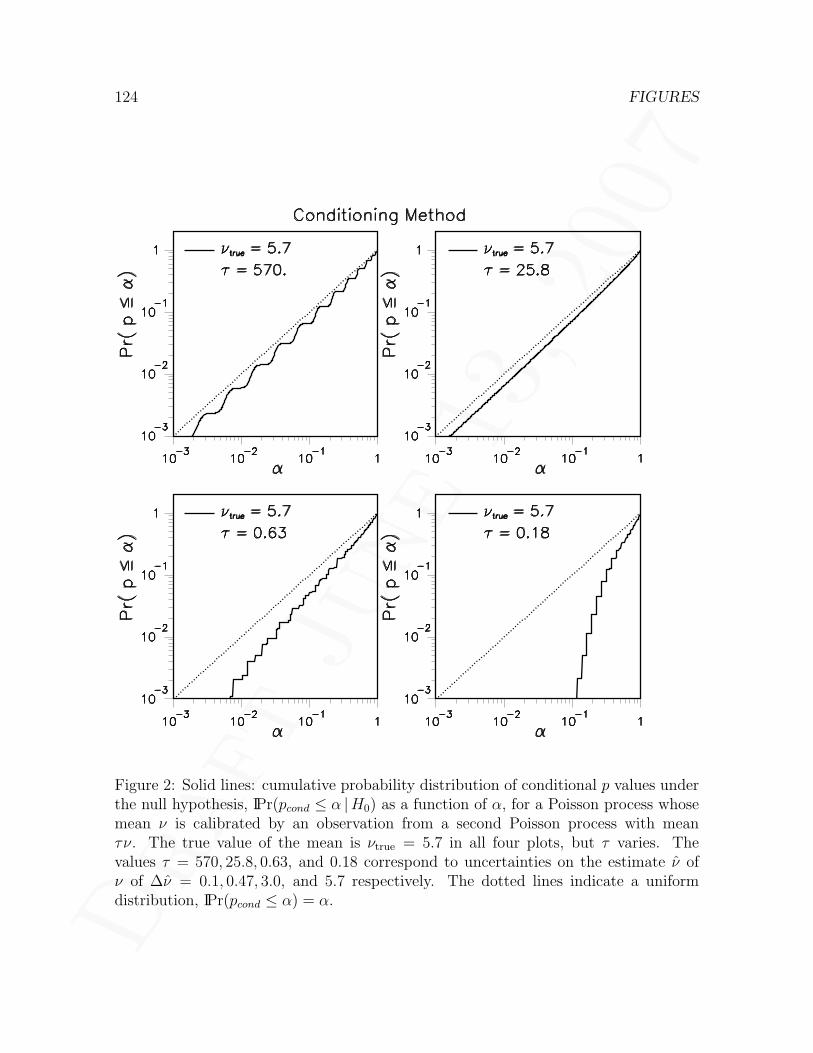
Dra

ftJu

ne13

,20

07

124 FIGURES

Figure 2: Solid lines: cumulative probability distribution of conditional p values underthe null hypothesis, IPr(pcond ≤ α |H0) as a function of α, for a Poisson process whosemean ν is calibrated by an observation from a second Poisson process with meanτν. The true value of the mean is νtrue = 5.7 in all four plots, but τ varies. Thevalues τ = 570, 25.8, 0.63, and 0.18 correspond to uncertainties on the estimate ν ofν of ∆ν = 0.1, 0.47, 3.0, and 5.7 respectively. The dotted lines indicate a uniformdistribution, IPr(pcond ≤ α) = α.

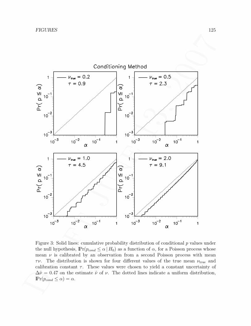
Dra

ftJu

ne13

,20

07

FIGURES 125

Figure 3: Solid lines: cumulative probability distribution of conditional p values underthe null hypothesis, IPr(pcond ≤ α |H0) as a function of α, for a Poisson process whosemean ν is calibrated by an observation from a second Poisson process with meanτν. The distribution is shown for four different values of the true mean νtrue andcalibration constant τ . These values were chosen to yield a constant uncertainty of∆ν = 0.47 on the estimate ν of ν. The dotted lines indicate a uniform distribution,IPr(pcond ≤ α) = α.

Dra

ftJu

ne13

,20

07

126 FIGURES

Figure 4: Tail probability of the likelihood ratio statistic under the null hypothesis,equation (4.3.18), as a function of the Poisson mean ν, for four different values of theGaussian uncertainty ∆ν. The cutoff constant c in the equation is here set equal to−2 lnλ(nobs, xobs). For ∆ν = 0.1, 0.47, 3.0, and 5.7, this yields c = 5.25, 5.02, 2.11, and0.91 respectively. The dashed lines indicate the asymptotic values (ν →∞) of the tailprobability.

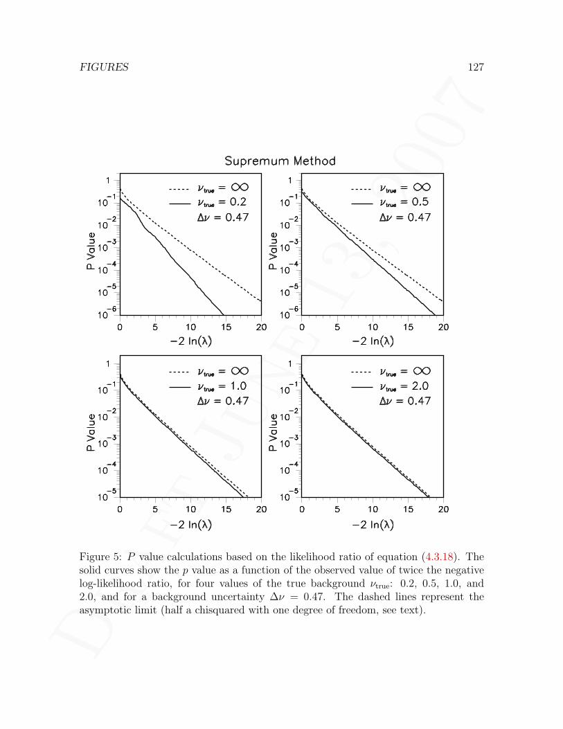
Dra

ftJu

ne13

,20

07

FIGURES 127

Figure 5: P value calculations based on the likelihood ratio of equation (4.3.18). Thesolid curves show the p value as a function of the observed value of twice the negativelog-likelihood ratio, for four values of the true background νtrue: 0.2, 0.5, 1.0, and2.0, and for a background uncertainty ∆ν = 0.47. The dashed lines represent theasymptotic limit (half a chisquared with one degree of freedom, see text).

Dra

ftJu

ne13

,20

07

128 FIGURES

Figure 6: Null hypothesis cumulative probability distribution of p values calculatedwith the likelihood ratio method. The solid lines show the distribution for a truebackground νtrue = 5.7, and for four values of the background uncertainty ∆ν: 0.1,0.47, 3.0, and 5.7. Each curve was obtained from a run of 107 Monte Carlo pseudo-experiments. The dotted lines represent a uniform distribution.

Dra

ftJu

ne13

,20

07

FIGURES 129

Figure 7: Null hypothesis cumulative probability distribution of p values calculatedwith the likelihood ratio method. The solid lines show the distribution for four values ofthe true background νtrue: 0.2, 0.5, 1.0, and 2.0, and for a background uncertainty ∆ν =0.47. Each curve was obtained from a run of 107 Monte Carlo pseudo-experiments. Thedotted lines represent a uniform distribution.

Dra

ftJu

ne13

,20

07

130 FIGURES

Figure 8: Null hypothesis survivor functions of the likelihood ratio statistic when boththe primary and subsidiary measurements have Poisson pdf’s. The true value of theprimary Poisson mean is varied from 0.57 to 57.0, and the ratio τ of the subsidiary tothe primary mean is varied from 1 to 1000. The dashed lines indicate the asymptoticsurvivor function, half a chisquared for one degree of freedom.

Dra

ftJu

ne13

,20

07

FIGURES 131

Figure 9: Likelihood ratio tail probability versus background mean, when both theprimary and auxiliary measurements have Poisson likelihood functions. The numberof observed events is n = 10 in the primary experiment and m = 7 in the auxiliaryone. The ratio of auxiliary to primary background means is τ = 16.5. The dottedline indicates the level of the supremum p value, whereas the dashed line marks theasymptotic p value.

Dra

ftJu

ne13

,20

07

132 FIGURES

Figure 10: Solid lines: cumulative probability distributions, under the null hypothesis,of p values calculated with the confidence interval method. The true background νtrue

is set at 5.7, whereas the background uncertainty ∆ν is varied from 0.1 to 5.7. A 6σconfidence upper limit on νtrue is used to calculate pβ (β = 1.97 × 10−9). Each solidcurve was obtained from a sample of 106 Monte Carlo experiments. The dashed linesshow the corresponding null distributions of supremum p values, and the dotted linesrepresent uniform distributions.

Dra

ftJu

ne13

,20

07

FIGURES 133

Figure 11: Solid lines: cumulative probability distributions, under the null hypothesis,of p values calculated with the confidence interval method. The true background νtrue

is varied from 0.2 to 2.0, whereas the background uncertainty ∆ν is kept fixed at 0.47.A 6σ confidence upper limit on νtrue is used to calculate pβ (β = 1.97 × 10−9). Eachsolid curve was obtained from a sample of 106 Monte Carlo experiments. The dashedlines show the corresponding null distributions of supremum p values, and the dottedlines represent uniform distributions.

Dra

ftJu

ne13

,20

07

134 FIGURES

Figure 12: Cumulative probability distribution, under the null hypothesis, of p valuescalculated with the confidence interval method. In these two plots, the null distributionis compared for two different confidence levels of the nuisance parameter interval: 6σor 1.97× 10−9 (solid curves), and 3σ or 2.70× 10−3 (dashed curves). The dotted linesrepresent a uniform distribution. The test statistic used to calculate confidence intervalp values is the likelihood ratio λ (top plot), and the maximum likelihood estimate µ ofthe signal (bottom plot).

Dra

ftJu

ne13

,20

07

FIGURES 135

Figure 13: Cumulative probability distributions of plug-in p values (dashed lines) andadjusted plug-in p values (solid lines) under the null hypothesis, for a Poisson processwhose mean has a Gaussian uncertainty ∆ν. The true value of the mean is νtrue = 5.7in all four plots, but ∆ν varies from 0.1 to 5.7. The dotted lines indicate a uniformdistribution, IPr(pplug ≤ α) = α.

Dra

ftJu

ne13

,20

07

136 FIGURES

Figure 14: Cumulative probability distributions of plug-in p values (dashed lines) andadjusted plug-in p values (solid lines) under the null hypothesis, for a Poisson processwhose mean has a Gaussian uncertainty ∆ν = 0.47. The distributions are shownfor four different values of the true mean νtrue. The dotted lines indicate a uniformdistribution, IPr(pplug ≤ α) = α.

Dra

ftJu

ne13

,20

07

FIGURES 137

Figure 15: Solid lines: cumulative probability distribution of fiducial p values under thenull hypothesis, for a Poisson process whose mean is known with a Gaussian uncertainty∆ν. The true value of the mean is νtrue = 5.7 in all four plots, but ∆ν varies from 0.1to 5.7. The dotted lines represent a uniform distribution.

Dra

ftJu

ne13

,20

07

138 FIGURES

Figure 16: Solid lines: cumulative probability distribution of fiducial p values under thenull hypothesis, for a Poisson process whose mean is known with a Gaussian uncertainty∆ν = 0.47. The distribution is shown for four different values of the true mean νtrue.The dotted lines indicate a uniform distribution.

Dra

ftJu

ne13

,20

07

FIGURES 139

Figure 17: Solid lines: cumulative probability distribution of prior-predictive p valuesunder the null hypothesis, IPr(pprior ≤ α |H0) as a function of α, for a Poisson processwhose mean is known with an absolute Gaussian uncertainty ∆ν. The true value ofthe mean is νtrue = 5.7 in all four plots, but ∆ν varies from 0.1 to 5.7. The dotted linesindicate a uniform distribution, IPr(pprior ≤ α) = α.

Dra

ftJu

ne13

,20

07

140 FIGURES

Figure 18: Solid lines: cumulative probability distribution of prior-predictive p valuesunder the null hypothesis, IPr(pprior ≤ α |H0) as a function of α, for a Poisson processwhose mean is known with an absolute Gaussian uncertainty ∆ν = 0.47. The distribu-tion is shown for four different values of the true mean νtrue. The dotted lines indicatea uniform distribution, IPr(pprior ≤ α) = α.

Dra

ftJu

ne13

,20

07

FIGURES 141

Figure 19: Comparison of the truncated Gaussian, gamma, and log-normal prior den-sities for the background in the X(3872) analysis. All three curves have the same meanand width. Plot (a) emphasizes differences in the tails, whereas plot (b) emphasizesdifferences around the maximum.

Dra

ftJu

ne13

,20

07

142 FIGURES

Figure 20: Solid lines: cumulative probability distribution of prior-predictive p valuesunder the null hypothesis, IPr(pprior ≤ α |H0) as a function of α, for a Poisson processwhose mean is known with a relative Gaussian uncertainty δ. The true value of themean is νtrue = 5.7 in all four plots, but δ varies from 0.0175 to 1.0. The dotted linesindicate a uniform distribution, IPr(pprior ≤ α) = α.

Dra

ftJu

ne13

,20

07

FIGURES 143

Figure 21: Solid lines: cumulative probability distribution of prior-predictive p valuesunder the null hypothesis, IPr(pprior ≤ α |H0) as a function of α, for a Poisson processwhose mean is known with a relative Gaussian uncertainty δ. The product δ × νtrue

is constant in all four plots and equals 0.47. The dotted lines indicate a uniformdistribution, IPr(pprior ≤ α) = α.

Dra

ftJu

ne13

,20

07

144 FIGURES

Figure 22: Solid lines: cumulative probability distribution of posterior-predictive pvalues under the null hypothesis, IPr(ppost ≤ α |H0) as a function of α, for a Poissonprocess whose mean is known with a Gaussian uncertainty ∆ν. The true value of themean is νtrue = 5.7 in all four plots, but ∆ν varies from 0.1 to 5.7. The dotted linesindicate a uniform distribution, IPr(ppost ≤ α) = α.

Dra

ftJu

ne13

,20

07

FIGURES 145

Figure 23: Solid lines: cumulative probability distribution of posterior-predictive pvalues under the null hypothesis, IPr(ppost ≤ α |H0) as a function of α, for a Poissonprocess whose mean is known with a Gaussian uncertainty ∆ν = 0.47. The distributionis shown for four different values of the true mean νtrue. The dotted lines indicate auniform distribution, IPr(ppost ≤ α) = α.

Dra

ftJu

ne13

,20

07

146 FIGURES

Figure 24: Solid lines: cumulative probability distribution of posterior-predictive pvalues under the null hypothesis and with respect to the prior-predictive measure, i.e.IPrpp(ppost ≤ α |H0) versus α, for a Poisson process with a Gaussian prior on the mean.The mean of the prior is x0 = 5.7 in all four plots, and its width varies from 0.1 to 5.7.The dotted lines indicate exact uniformity, IPrpp(ppost ≤ α) = α.

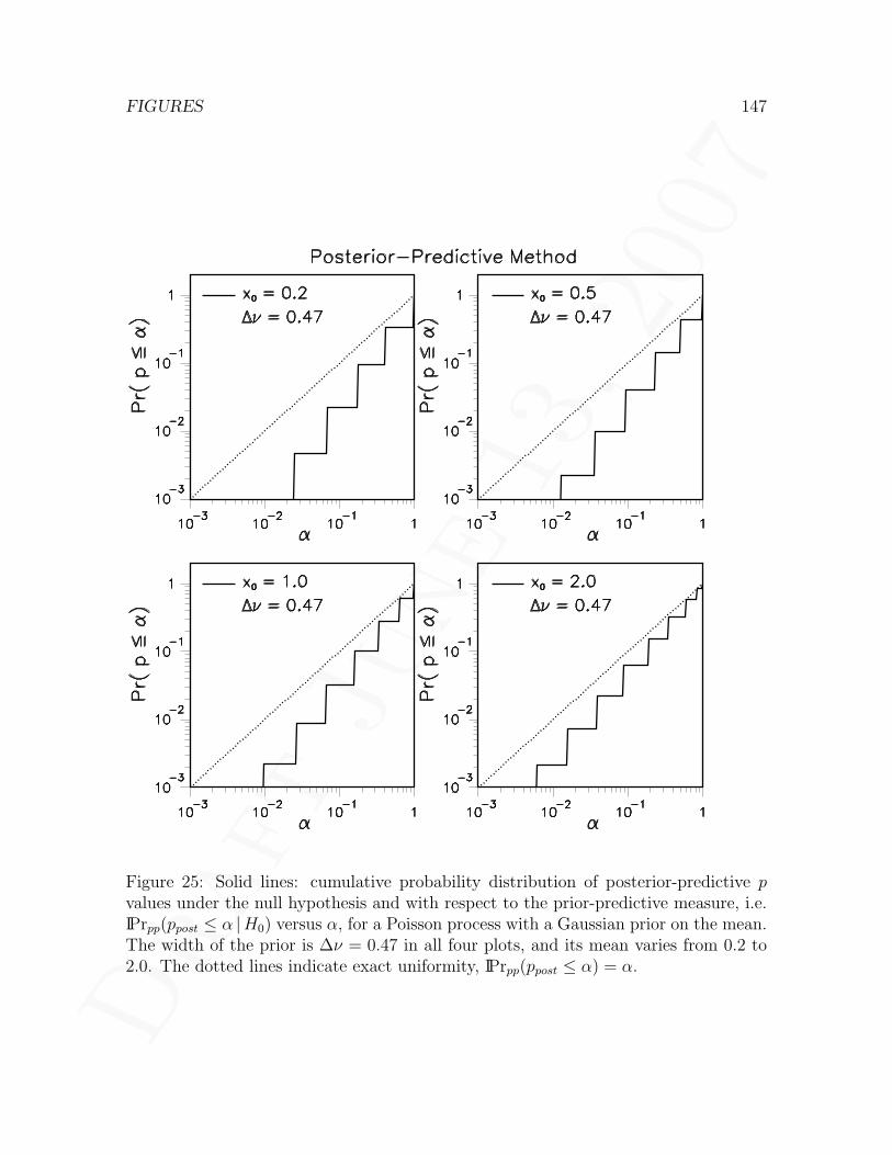
Dra

ftJu

ne13

,20

07

FIGURES 147

Figure 25: Solid lines: cumulative probability distribution of posterior-predictive pvalues under the null hypothesis and with respect to the prior-predictive measure, i.e.IPrpp(ppost ≤ α |H0) versus α, for a Poisson process with a Gaussian prior on the mean.The width of the prior is ∆ν = 0.47 in all four plots, and its mean varies from 0.2 to2.0. The dotted lines indicate exact uniformity, IPrpp(ppost ≤ α) = α.

Dra

ftJu

ne13

,20

07

148 FIGURES

Figure 26: Power of supremum (solid), adjusted plug-in (dashed), fiducial (dotted),and prior-predictive (dot-dashed) p values for testing for the presence of a Poissonsignal on top of a Poisson background whose mean νtrue has a Gaussian uncertainty∆ν. The power is calculated for a test level of α = 5% and is plotted as a function ofthe true signal strength.

Dra

ftJu

ne13

,20

07

FIGURES 149

Figure 27: P value plot of electroweak observables compared with standard modelpredictions, as listed in the 2004 edition of the Particle Data Group’s review of particleproperties (Table 10.4). There are 37 data points, and the dotted line is a straight linethrough the origin and with a slope of 37.

Dra

ftJu

ne13

,20

07

150 FIGURES

Figure 28: Top: spectrum used to generate pseudo-experiments for figures 29, 30, 31,and 33. Bottom: spectrum used to generate pseudo-experiments for figure 32.

Dra

ftJu

ne13

,20

07

FIGURES 151

Figure 29: Chisquared distributions obtained from an ensemble of 20,000 pseudo-experiments. In each experiment, a binned spectrum is generated by Gaussian fluc-tuations from a fixed quadratic polynomial background. The generated spectrum isthen fitted to a quadratic polynomial (H0 fit, top left) and to a quartic polynomial(H1 fit, top right). The chisquared difference between these two fits is shown in thebottom plot. The pseudo-experiment distributions (solid histograms) are compared tochisquared curves for the appropriate number of degrees of freedom (dashed lines). Inthe definition of the fit chisquared, each bin is weighted by the inverse of the varianceof the Gaussian fluctuations used to generate its contents.

Dra

ftJu

ne13

,20

07

152 FIGURES

Figure 30: Same as figure 29, except that:1. the spectrum observed in each experiment is generated by Poisson fluctuations from

the fixed background;

2. in the definition of the fit chisquared, each bin is weighted by the inverse of theobserved bin contents (Neyman’s chisquared).

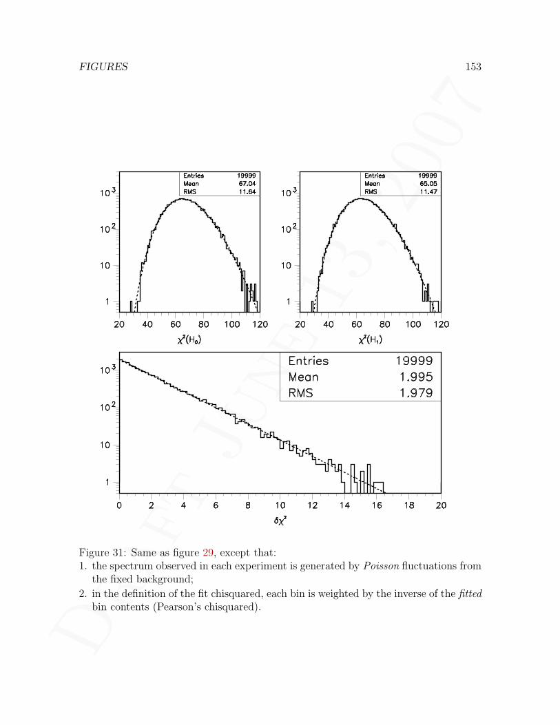
Dra

ftJu

ne13

,20

07

FIGURES 153



2. in the definition of the fit chisquared, each bin is weighted by the inverse of the fittedbin contents (Pearson’s chisquared).

Dra

ftJu

ne13

,20

07

154 FIGURES



2. the fixed background consists of a Gaussian resonance on top of a quadratic back-ground (six parameters);

3. in the definition of the fit chisquared, each bin is weighted by the inverse of the fittedbin contents (Pearson’s chisquared).

Dra

ftJu

ne13

,20

07

FIGURES 155



2. The H1 fit (top right) is to a fixed-width Gaussian resonance on top of a quadraticbackground (five parameters);

3. in the definition of the fit chisquared, each bin is weighted by the inverse of the fittedbin contents (Pearson’s chisquared);

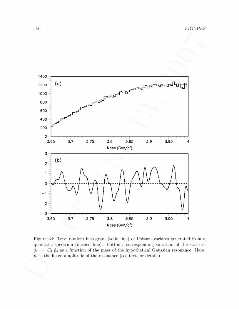
Dra

ftJu

ne13

,20

07

156 FIGURES

Figure 34: Top: random histogram (solid line) of Poisson variates generated from aquadratic spectrum (dashed line). Bottom: corresponding variation of the statisticq4 = C4 p4 as a function of the mass of the hypothetical Gaussian resonance. Here,p4 is the fitted amplitude of the resonance (see text for details).

Dra

ftJu

ne13

,20

07

FIGURES 157

Figure 35: Distribution densities of the one-sided (a) and two-sided (b) delta-chisquaredstatistics, respectively δX2

sup(1s) and δX2sup(2s), for a set of pseudo-experiments simulat-

ing the X(3872) analysis. For the solid histograms, the delta-chisquareds were calcu-lated by the finite-sample bootstrap method described in section 6.2.2. For the dashedhistograms, the delta-chisquareds were obtained via the grid search implementation ofthe asymptotic bootstrap method described in section 6.2.3. The statistics boxes applyto the solid histograms.

Dra

ftJu

ne13

,20

07

158 FIGURES

Figure 36: Top: integrand of the constant K of equation (6.2.6), as a function of theintegration variable θ. Bottom: survivor function of the one-sided delta-chisquaredstatistic δX2

sup(1s). The solid line was obtained from a set of pseudo-experiments gener-

ated with the finite-sample bootstrap method (see section 6.2.2), and is compared withthe upper bound of equation (6.2.5) in the text (dot-dashes), and with half-chisquareddistributions for one and two degrees of freedom (dashes and dots, respectively).

Dra

ftJu

ne13

,20

07

FIGURES 159

Figure 37: Power of one-sided tests when nuisance parameters are present under thealternative but not under the null. For this example calculation, the background spec-trum of Figure 28(a) was used, and a Gaussian signal with a width of 4.3 MeV/c2 wassuperimposed at a location of 3872 MeV/c2. Five power functions are plotted as afunction of the number of signal events: the χ2 goodness-of-fit test (dot-dashes), theAveLR test (dots), the ExpLR and SupLR tests (indistinguishable from each other andshown by dashes), and the LR test for the case where the signal location is known apriori (solid). All power functions are evaluated assuming a significance level of 0.27%.(SupLR is another name for δX2

sup, which for one-sided tests is given by equation (6.2.3)in the text.)

Dra

ftJu

ne13

,20

07

160 FIGURES

Figure 38: Same as Figure 37, but for two-sided tests.

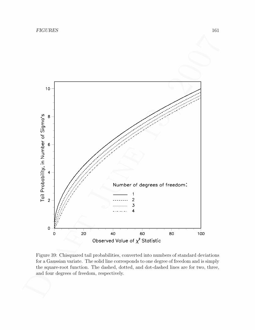
Dra

ftJu

ne13

,20

07

FIGURES 161

Figure 39: Chisquared tail probabilities, converted into numbers of standard deviationsfor a Gaussian variate. The solid line corresponds to one degree of freedom and is simplythe square-root function. The dashed, dotted, and dot-dashed lines are for two, three,and four degrees of freedom, respectively.

Dra

ftJu

ne13

,20

07

162 FIGURES

Figure 40: Coverage of a standard search and discovery procedure in HEP. One istesting the mean, constrained to be positive, of a Gaussian pdf with unit width. Thediscovery threshold is set at 5σ. When no discovery is claimed, an upper limit withconfidence level α1 is calculated. Otherwise a two-sided interval with confidence levelα2 is reported. The solid lines show the coverage of this procedure for various choices ofα1 and α2. The dashed (dotted) lines show the 95% (68%) level. Plot (d) correspondsto the usual choices.

Dra

ftJu

ne13

,20

07

FIGURES 163

Figure 41: Conditional coverage of a standard search and discovery procedure in HEP.One is interested in the mean µ, constrained to be positive, of a Gaussian pdf withunit width. The discovery threshold is set at 5σ. When no discovery is claimed, a95% confidence level upper limit on µ is calculated. Otherwise a 68% confidence leveltwo-sided interval is reported. The solid line shows the coverage of the upper limit withrespect to the subset of experiments claiming no discovery. The dashed line shows thecoverage of the two-sided interval with respect to the subset of experiments claimingdiscovery.

Dra

ftJu

ne13

,20

07

164 FIGURES

Figure 42: Neyman construction of conditional intervals for the problem of determiningthe mean µ, constrained to be positive, of a Gaussian pdf, when one observation x hasbeen made. The dotted line indicates the critical value xc = nσ of x: observationsabove that value lead to rejection of the null hypothesis H0 : µ = 0. The solid line tothe left of xc is the conditional 95% C.L. upper limit on µ, given x < xc. The two solidlines to the right of xc mark the boundaries of the conditional 68% C.L. central intervalon µ, given x ≥ xc. The dashed lines are the corresponding unconditional intervals.

Dra

ftJu

ne13

,20

07

FIGURES 165

Figure 43: Neyman construction of conditional intervals for the problem of determiningthe mean µ, constrained to be positive, of a Gaussian pdf, when one observation x hasbeen made. The dotted line indicates the critical value xc = nσ of x: observationsabove that value lead to rejection of the null hypothesis H0 : µ = 0. The solid lines tothe left (right) of xc mark the boundaries of the conditional 95% (68%) C.L. intervalsfor µ, using a likelihood ratio ordering rule.[46] The dashed lines are the correspondingunconditional intervals.

Dra

ftJu

ne13

,20

07

166 FIGURES

Figure 44: Result of 20,000 pseudo-experiments in which a mass spectrum, drawnfrom a quadratic polynomial template, is fit to two models: the fit 1 model is a simplequadratic polynomial, whereas the fit 2 model is the sum of a quadratic polynomialand a fixed-width Gaussian. The width of the Gaussian is comparable to the bin widthof the mass spectrum. Plots (a) and (c) are distributions of the mean of the Gaussianfrom fit 2, and plots (b) and (d) are distributions of the delta-chisquared between thetwo fits. For plots (a) and (b), the initial value of the Gaussian mean given to thefitter (minuit) for fit 2 was 3.825. For plots (c) and (d), fit 2 was repeated for seventyinitial values of the Gaussian mean, equally spaced between 3.65 and 4.00, and onlythe fit with the lowest chisquared was retained. The amplitude of the Gaussian in fit2 was always required to be positive.

Dra

ftJu

ne13

,20

07

FIGURES 167

Figure 45: Result of pseudo-experiments in which a mass spectrum, drawn from thequadratic template of Figure 28b, is fit to a quadratic polynomial (fit 1) and to thesum of a quadratic polynomial and a fixed-width Gaussian resonance (fit 2). The solidhistograms show distributions of the delta-chisquared between fits 1 and 2 for differentconstraints on the mean of the Gaussian resonance. For plot (a), that mean can beanywhere between 3.65 and 4.00; for plot (b), between 3.825 and 4.00; for plot (c),between 3.870 and 3.875; for plots (d1) and (d2), the mean is kept fixed at 3.8714.The amplitude of the Gaussian resonance is allowed to be positive or negative in allplots except (d2), where it is constrained to be positive. The dotted (dashed) lines arechisquared densities for one (two) degree(s) of freedom.

Dra

ftJu

ne13

,20

07

168 REFERENCES

References

[1] Abe, F., et al. (CDF Collaboration), “Evidence for top quark production in ppcollisions at

√s = 1.8 TeV,” Phys. Rev. D50, 2966 (1994). 18

[2] Acosta, D., et al. (CDF Collaboration), “Observation of the narrow stateX(3872) → J/ψπ+π− in pp collisions at

√s = 1.96 TeV,” Phys. Rev. Lett. 93,

072001 (2004). 15, 16, 97, 98, 103

[3] Andrews, D. W. K., and Ploberger, W., “Optimal tests when a nuisance parameteris present only under the alternative,” Econometrica 62, 1383 (1994). 104

[4] Andrews, D. W. K., and Ploberger, W., “Admissibility of the likelihood ratio testwhen a nuisance parameter is present only under the alternative,” Ann. Statist.23, 1609 (1995). 103

[5] Basu, D., “On the elimination of nuisance parameters,” J. Amer. Statist. Assoc.72, 355 (1977). 43

[6] Bayarri, M. J., and Berger, J. O., “Measures of surprise in Bayesian analysis,”ISDS Discussion Paper 97-46, Duke University (1997); see http://ftp.isds.

duke.edu/WorkingPapers/97-46.html. 11, 35, 76, 82

[7] Beran, R., “Prepivoting test statistics: a bootstrap view of asymptotic refine-ments,” J. Amer. Statist. Assoc. 83, 687 (1988). 98

[8] Bayarri, M. J., and Berger, J. O., “P-values for composite null models [with discus-sion],” J. Amer. Statist. Assoc. 95, 1127 (2000); also available as ISDS DiscussionPaper 98-40 (1998), http://ftp.isds.duke.edu/WorkingPapers/98-40.html.75, 82

[9] Berger, J. O., “Statistical decision theory and Bayesian analysis,” 2nd edition,Springer-Verlag New York, Inc., 1985 (617pp). 35

[10] Berger, J. O., and Sellke, T., “Testing a point null hypothesis: the irreconcilabilityof p values and evidence [with discussion],” J. Amer. Statist. Assoc. 82, 112 (1987).13, 20

[11] Berger, J. O., and Sellke, T., “Testing a point null hypothesis: the irreconcilabilityof p values and evidence. Rejoinder,” J. Amer. Statist. Assoc. 82, 135 (1987). 34

[12] Berger, J. O., and Delampady, M., “Testing precise hypotheses,” Statist. Sci. 2,317 (1987). 23

[13] Berger, R. L., and Boos, D. D., “P values maximized over a confidence set for thenuisance parameter,” J. Amer. Statist. Assoc. 89, 1012 (1994). 43, 54

http://ftp.isds.duke.edu/WorkingPapers/97-46.html



Dra

ftJu

ne13

,20

07

REFERENCES 169

[14] Berkson, J., “Minimum chi-square, not maximum likelihood,” Ann. Statist. 8, 457(1980). 99

[15] Bernardo, J. M., and Rueda, R., “Bayesian hypothesis testing: a referenceapproach,” Int. Statist. Review 70, 351 (2002); see also http://www.uv.es/∼bernardo/publications.html. 32, 37

[16] Bernardo, J. M., “Reference analysis,” Handbook of Statistics 25 (D.K. Dey andC.R. Rao, eds.), Amsterdam: Elsevier, pg 17 (2005). 38, 80

[17] Berry, S. M., and Viele, K., “Adjusting the α level for sample size,” CarnegieMellon University Department of Statistics Technical Report 635 (1995); http://www.stat.cmu.edu/tr/tr635/tr635.ps. 29

[18] Box, G. E. P., “Sampling and Bayes’ inference in scientific modelling and robust-ness [with discussion],” J. R. Statist. Soc. A 143, 383 (1980). 69

[19] Carlin, B. P., and Louis, T. A., “Bayes and empirical Bayes methods for dataanalysis,” Monographs on Statistics and Applied Probability 69, Chapman andHall, 1996 (399pp). 76

[20] Casella, G., and Berger, R. L., “Reconciling Bayesian and frequentist evidence inthe one-sided testing problem [with discussion],” J. Amer. Statist. Assoc. 82, 106(1987). 20

[21] Casella, G., and Berger, R. L., “Statistical Inference,” 2nd edition, Duxbury, PacificGrove, CA, 2002 (660pp). 15, 16, 34, 46

[22] Chang, D., Chang, W.-F., and Ma, E., “Alternative interpretation of the FermilabTevatron top events,” Phys. Rev. D59, 091503 (1999). 12

[23] Cheng, R. C. H., and Traylor, L., “Non-regular maximum likelihood problems,”J. R. Statist. Soc. B 57, 3 (1995). 105

[24] Chernoff, H., “On the distribution of the likelihood ratio,” Ann. Math. Statist.24, 573 (1954). 51

[25] Choi, S. K., et al. (Belle Collaboration), “Observation of a narrow charmonium-like state in exclusive B± → K±π+π−J/ψ decays,” Phys. Rev. Lett. 91, 262001(2003). 96, 105

[26] Cousins, R. D., “Annotated bibliography of some papers on combining signifi-cances or p-values,” arXiv:0705.2209v1 [physics.data-an] 15 May 2007. 94

[27] Cox, D. R., “The continuity correction,” Biometrika 57, 217 (1970). 77

[28] Cramer, H., “Mathematical Methods of Statistics,” Princeton University Press,1946 (575pp). 120

http://www.uv.es/~bernardo/publications.html

http://www.uv.es/~bernardo/publications.html

http://www.stat.cmu.edu/tr/tr635/tr635.ps

http://www.stat.cmu.edu/tr/tr635/tr635.ps

Dra

ftJu

ne13

,20

07

170 REFERENCES

[29] Currie, L. A., Eijgenhuijsen, E. M., and Klouda, G. A., “On the validity of thePoisson hypothesis for low-level counting: investigation of the distributional char-acteristics of background radiation with the NIST individual pulse counting sys-tem,” Radiocarbon 40, 113 (1998). 15

[30] Darling, D. A., and Robbins, H., “Iterated logarithm inequalities,” Proc. Nat.Acad. Sci. 57, 1188 (1967). 26

[31] Davidson, R., and MacKinnon, J. G., “Econometric theory and methods,” OxfordUniversity Press, New York, 2004 (750 pp). 99

[32] Davies, R. B., “Hypothesis testing when a nuisance parameter is present onlyunder the alternative,” Biometrika 64, 247 (1977). 103

[33] Davies, R. B., “Hypothesis testing when a nuisance parameter is present onlyunder the alternative,” Biometrika 74, 33 (1987). 103

[34] Davison, A. C., Hinkley, D. V., and Young, G. A., “Recent developments in boot-strap methodology,” Statist. Sci. 18, 141 (2003). 63

[35] Dawid, A. P., and Dickey, J. M., “Likelihood and Bayesian inference from selec-tively reported data,” J. Amer. Statist. Assoc. 72, 845 (1977). 110

[36] Delampady, M., and Berger, J. O., “Lower bounds on Bayes factors for multino-mial distributions, with application to chi-squared tests of fit,” Ann. Statist. 18,1295 (1990). 36

[37] Demortier, L., “Constructing Ensembles of Pseudo-Experiments,” in Proceed-ings of the PhyStat2003 Conference, SLAC, September 8–11, 2003; see alsoarXiv:physics/0312100 v2 (16 Dec 2003). 21, 25, 96

[38] Demortier, L., and Lyons, L., “Everything you always wanted to know aboutpulls,” CDF/ANAL/PUBLIC/5776, Version 2.10 (February 26, 2002). 122

[39] Dieudonne, J., “Calcul infinitesimal,” Hermann, Paris, 1968 (479pp). 112

[40] Dorigo T., and Schmitt, M., “On the significance of the dimuon mass bump andthe greedy bump bias,” CDF/DOC/TOP/CDFR/5239 (February 26, 2000). 122

[41] Eadie, W. T., Drijard, D., James, F. E., Roos, M., and Sadoulet, B., “StatisticalMethods in Experimental Physics,” North Holland, Amsterdam and London, 1971(291pp). 99

[42] Efron, B., and Tibshirani, R., “The problem of regions,” Ann. Statist. 26, 1687(1998); see also http://www-stat.stanford.edu/∼tibs/ftp/regions.ps. 30,32

http://www-stat.stanford.edu/~tibs/ftp/regions.ps

Dra

ftJu

ne13

,20

07

REFERENCES 171

[43] Eidelman, S., et al. (Particle Data Group), “Review of Particle Physics,” Phys.Lett. B 592, 1 (2004). 91, 92

[44] Evans, M., “Bayesian inference procedures derived via the concept of relativesurprise,” Commun. Statist. 26, 1125 (1997); see also http://www.utstat.

utoronto.ca/mikevans/. 37

[45] Fan, J., Hung, H.-N., and Wong, W.-H., “Geometric understanding of likelihoodratio statistics,” J. Amer. Statist. Assoc. 95, 836 (2000). 95

[46] Feldman, G. J., and Cousins, R. D., “Unified approach to the classical statisticalanalysis of small signals,” Phys. Rev. D57, 3873 (1998). 34, 107, 108, 110, 165

[47] Forsythe, G. E., “Generation and Use of Orthogonal Polynomials for Data Fittingwith a Digital Computer,” J. Soc. Indust. Appl. Math. 5, 74 (1957). 119

[48] Fraser, D. A. S., Reid, N., and Wong, A. C. M., “Inference for bounded parame-ters,” Phys. Rev. D 69, 033002 (2004). 33

[49] Gallant, A. R., “Testing a nonlinear regression specification: a nonregular case,”J. Amer. Statist. Assoc. 72, 523 (1977). 101

[50] Gelman, A., Meng, X.-L., and Stern, H., “Posterior predictive assessment of modelfitness via realized discrepancies,” Statist. Sinica 6, 733 (1996). 11

[51] Good, I. J., “The Bayes/non-Bayes compromise: a brief review,” J. Amer. Statist.Assoc. 87, 597 (1992). 26, 27, 32

[52] Goutis, C., Casella, G., and Wells, M. T., “Assessing evidence in multiple hy-potheses,” J. Amer. Statist. Assoc. 91, 1268 (1996). 93

[53] Hannig, J., Iyer, H., and Patterson, P. L., “On fiducial generalized confidence in-tervals,” J. Amer. Statist. Assoc. 101, 254 (2006); Colorado State University De-partment of Statistics Technical Report 2004/12; http://www.stat.colostate.edu/∼hari/fiducial/fgpq.pdf. 63, 64

[54] Hannig, J., “On fiducial inference — the good, the bad and the ugly,” ColoradoState University Department of Statistics Technical Report 2006/ 63, 68

[55] Hansen, B. E., “Inference when a nuisance parameter is not identified under thenull hypothesis,” Econometrica 64, 413 (1996).

[56] Hansen, B. E., “Challenges for econometric model selection,” Econometric Theory21, 60 (2005). 111

[57] Hjort, N. L., Dahl, F. A., and Steinbakk, G. H., “Post-processing posterior pre-dictive p values,” J. Amer. Statist. Assoc. 101, 1157 (2006). 87

http://www.utstat.utoronto.ca/mikevans/

http://www.utstat.utoronto.ca/mikevans/

http://www.stat.colostate.edu/~hari/fiducial/fgpq.pdf

http://www.stat.colostate.edu/~hari/fiducial/fgpq.pdf

Dra

ftJu

ne13

,20

07

172 REFERENCES

[58] Hochberg, Y., “A sharper Bonferroni procedure for multiple tests of significance,”Biometrika 75, 800 (1988). 94

[59] Hubbard, R., and Bayarri, M. J., “P values are not error probabilities,” ISDSDiscussion Paper 03-26 (2003), http://ftp.isds.duke.edu/WorkingPapers/

03-26.html. 9, 19

[60] Iyer, H. K., and Patterson, P. D., “A recipe for constructing generalized piv-otal quantities and generalized confidence intervals,” Colorado State UniversityDepartment of Statistics Technical Report 2002/10; also at http://www.stat.

colostate.edu/research/2002 10.pdf. 63, 64

[61] Johnson, V. E., “A Bayesian χ2 test for goodness-of-fit,” Ann. Statist. 32, 2361(2004). 38

[62] King, M. L., and Shively, T. S., “Locally optimal testing when a nuisance param-eter is present only under the alternative,” Rev. Econom. Statist. 75, 1 (1993).105

[63] Leeb, H., and Potscher, B., “Model selection and inference: facts and fic-tion,” Econometric Theory 21, 21 (2005); see also http://www.stat.yale.edu/∼hl284/ETAnniv.pdf. 110

[64] Lehmann, E. L., “Elements of Large-Sample Theory,” Springer-Verlag, New York,Inc., 1999 (Corrected second printing, 2001) (631 pp).

[65] Lejeune, M., and Faulkenberry, G. D., “A simple predictive density function,” J.Amer. Statist. Assoc. 77, 654 (1982). 83

[66] Leonard, T., and Hsu, J. S. J., “Bayesian Methods: An Analysis for Statisticiansand Interdisciplinary Researchers,” Cambridge University Press, 1999 (333pp). 76

[67] Lindley, D. V., “Introduction to probability and statistics from a Bayesian view-point. Part 2. Inference,” Cambridge University Press, 1965 (292pp). 35

[68] Linnemann, J. T., “Measures of significance in HEP and astrophysics,” in Pro-ceedings of the PhyStat2003 Conference, SLAC, September 8–11, 2003; see alsoarXiv:physics/0312059 v2 (12 Dec 2003). 73

[69] Lyons, L., private communication. 15, 19

[70] McCullagh, P., Comment on “The Roles of Conditioning in Inference,” by N. Reid;Statist. Sci. 10, 177 (1995). 70

[71] McLaren, C. E., Legler, J. M., and Brittenham, G. M., “The generalized χ2

goodness-of-fit test,” Statistician 43, 247 (1994). 30



http://www.stat.colostate.edu/research/2002_10.pdf

http://www.stat.colostate.edu/research/2002_10.pdf

http://www.stat.yale.edu/~hl284/ETAnniv.pdf

http://www.stat.yale.edu/~hl284/ETAnniv.pdf

Dra

ftJu

ne13

,20

07

REFERENCES 173

[72] Meeks, S. L., “Conditional estimation following tests,” Biometrika 66, 668 (1979).108

[73] Meng, X. L., “Posterior Predictive p-Values,” Ann. Statist. 22, 1142 (1994). 81,86, 88

[74] Newton, M. A., Geyer, C. J., “Bootstrap recycling: a Monte Carlo alternative tothe nested bootstrap,” J. Amer. Statist. Assoc. 89, 905 (1994). 60

[75] Neyman, J., “Basic ideas and some recent results of the theory of testing statisticalhypotheses,” J. R. Statist. Soc. 105, 292 (1942). 12

[76] Pilla, R. S., Loader, C., and Taylor, C. C., “New technique for finding needlesin haystacks: geometric approach to distinguishing between a new source andrandom fluctuations,” Phys. Rev. Lett. 95, 230202 (2005). 105

[77] Porteous, B. T., “Stochastic inequalities relating a class of log-likelihood ratiostatistics to their asymptotic χ2 distribution,” Ann. Statist. 17, 1723 (1989). 54

[78] Press, W. H., Teukolsky, S. A., Vetterling, W. T., and Flannery, B. P., “NumericalRecipes in C++, The Art of Scientific Computing,” 2nd ed., Cambridge UniversityPress, 2002 (1002pp). 44, 70

[79] Royall, R., “On the probability of observing misleading statistical evidence,” J.Amer. Statist. Assoc. 95, 760 (2000). 35

[80] Robins, J. M., van der Vaart, A., and Ventura, V., “Asymptotic Distribution ofP Values in Composite Null Models [with discussion],” J. Amer. Statist. Assoc.95, 1143 (2000). 38, 59, 62

[81] Roe, B. P., “Probability and Statistics in Experimental Physics,” 2nd edition,Springer-Verlag, New York, 2001 (264pp). 97

[82] Schervish, M., “P values: what they are and what they are not,” Amer. Statis-tician 50, 203 (1996); “A significance paradox,” Carnegie Mellon University De-partment of Statistics Technical Report 598r (1994); http://www.stat.cmu.edu/tr/tr598r/tr598r.html. 30

[83] Schweder, T., and Spjøtvoll, E., “Plots of P -values to evaluate many tests simul-taneously,” Biometrika 69, 493 (1982). 91

[84] Sellke, T., Bayarri, M. J., and Berger, J. O., “Calibration of p values for testingprecise null hypotheses,” Amer. Statistician 55, 62 (2001). 22, 33

[85] Seneta, E., and Chen, J. T., “Simple stepwise tests of hypotheses and multiplecomparisons,” Internat. Statist. Rev. 73, 21 (2005). 94

http://www.stat.cmu.edu/tr/tr598r/tr598r.html

http://www.stat.cmu.edu/tr/tr598r/tr598r.html

Dra

ftJu

ne13

,20

07

174 REFERENCES

[86] Shaffer, J. P., “Multiple hypothesis testing,” Annu. Rev. Psychol. 46, 561 (1995).94

[87] Silvapulle, M. J., “A test in the presence of nuisance parameters,” J. Amer. Statist.Assoc. 91, 1690 (1996); Correction, ibidem 92, 801 (1997). 54

[88] Simes, R. J., “An improved Bonferroni procedure for multiple tests of significance,”Biometrika 73, 751 (1986). 94

[89] Singh, K., and Berk, R. H., “A concept of type-2 p-value,” Statist. Sinica 4, 493(1994). 63

[90] Smyth, G. K., “Pearson’s goodness of fit statistic as a score test statistic,” inScience and Statistics: A Festschrift for Terry Speed, D. R. Goldstein (ed.), IMSLecture Notes — Monograph Series, Volume 40, Institute of Mathematical Statis-tics, Beachwood, Ohio, pg. 115-126 (2003); http://www.statsci.org/smyth/

pubs/goodness.pdf.

[91] Soric, B., “Statistical ‘discoveries’ and effect-size estimation,” J. Amer. Statist.Assoc. 84, 608 (1989). 15

[92] Storey, J. D., “A direct approach to false discovery rates,” J. R. Statist. Soc. 64,479 (2002). 94

[93] Stuart, A., and Ord, K., “Distribution Theory,” vol. 1 of “Kendall’s AdvancedTheory of Statistics,” 6th edition, Edward Arnold, London, 1994 (676pp). 18

[94] Stuart, A., Ord, K., and Arnold, S., “Classical Inference and the Linear Model,”vol. 2A of “Kendall’s Advanced Theory of Statistics,” 6th edition, Edward Arnold,London, 1999 (885pp). 49, 97

[95] Taylor, J. E., and Worsley, K. J., “Detecting sparse signals in random fields, withan application to brain mapping,” J. Amer. Statist. Assoc., accepted (2007); seealso http://www.math.mcgill.ca/keith/noniso/noniso.htm. 105

[96] Tierney, L., and Kadane, J. B., “Accurate approximations for posterior momentsand marginal densities,” J. Amer. Statist. Assoc. 81, 82 (1986). 113

[97] Tsui, K. W., and Weerahandi, S., “Generalized p-values in significance testing ofhypotheses in the presence of nuisance parameters,” J. Amer. Statist. Assoc. 84,602 (1989). Erratum: ibid. 86, 256 (1991). 63, 65

[98] Wilks, S. S., “The large-sample distribution of the likelihood ratio for testingcomposite hypotheses,” Ann. Math. Statist. 9, 60 (1938). 95

http://www.statsci.org/smyth/pubs/goodness.pdf

http://www.statsci.org/smyth/pubs/goodness.pdf

http://www.math.mcgill.ca/keith/noniso/noniso.htm

P Values: What They Are and How to Use Them - CDF - Fermilab

Documents

Transcript of P Values: What They Are and How to Use Them - CDF - Fermilab