P d th l tP d th l tPower and thermal managementPower and thermal management

Tajana Šimunić RosingTajana Šimunić Rosing

UCSD

MotivationMotivationPower consumption is a critical issue in system design today

Mobile systems want maximum battery lifetimeHigh performance systems need to reduce the electricity costsHigh performance systems need to reduce the electricity costs

• Power and cooling

Electricity cost devoted to powering and cooling USA data centers can power 10 Icelands!

TŠR

Power and Thermal ManagementPower and Thermal ManagementReducing power ≠ lower thermal densityPower management

Sleep states – DPMPerformance states – DVFS

Thermal managementThermal Hot Spots

• High leakage power• High leakage power• Degraded reliability• Increased interconnect resistivity

Spatial and Temporal GradientsSpatial and Temporal Gradients• Higher permanent failure rates• Timing failures• Increased interconnect delay and IR drop

TŠR

Increased interconnect delay and IR drop

Our Recent WorkOur Recent Work

Dynamic power management (DPM)O ti l t f t ti kl d• Optimal power management for stationary workloads

• Machine learning to adapt in non-stationary environments• Select among specialized policies• Use hardware performance counters to adapt• Use hardware performance counters to adapt

voltage/frequency settings at run time • Measured large power savings in real systems

Dynamic thermal management (DTM)• Workload scheduling:

• Comparison between power only and thermal management• Comparison between power only and thermal management• Runtime adaptation to get best temporal and spatial profiles• Negligible performance overhead

• Accurate run-time temperature estimation

TŠR

Accurate run time temperature estimation• Limited number of thermal sensors in suboptimal locations

DPM: Workload modeling - Idle StateDPM: Workload modeling - Idle State

11 10 100 1000

Hard Disk Trace

bE −1Pareto Distribution:

0 001

0.01

0.1

Tail

dist

ribut

ion Pareto

Experimental

WWW T

buser taE −⋅−= 1

0.0001

0.001T Exponential

WWW Trace

0.1

1

Telnet Trace

0.1

1

0.001

0.01

0.1

Experimental

Exponential 0.001

0.01 Experimental

Exponential

P t

TŠR

0.00010.01 0.1 1 10

Interarrival Time (s)

Pareto0.0001

0.01 0.1 1 10

Interarrival Time (s)

Pareto

DPM: TISMDP modelDPM: TISMDP model

Idle

departure Decision

A Q A Q=1A Q=2 arrival

Idle

i l

arrivaluniform

A,Qmax A,Q=1A,Q=2. . .

S,Q=1S,Qmax . . .arrival

S,Q=0no arrival

generalAssumptions: generalAssumptions:general distribution governs the first request arrival exponential distribution represents arrivals after the first arrivaluser, device and queue are stationaryuser, device and queue are stationary

Obtain globally optimal policy using linear programming

h d di k i hi f id l l li

TŠR

Measurements on hard disk within 11% of ideal oracle policyfactor of 2.4 lower than always-onfactor of 1.7 lower than default time-out

DPM: Hardware implementationDPM: Hardware implementationDPM: Hardware implementationDPM: Hardware implementation

Idle time Probability(ms) to sleep

Optimal PolicyOptimal PolicyLFSR for generating probability & policy logicController on entry to idle state:Controller on entry to idle state:

obtains a random number RND & finds a timeoutobtains a random number RND & finds a timeout (ms) to sleepjh p(jh)

0 0.0010 0.0020 0 12

obtains a random number RND & finds a timeout obtains a random number RND & finds a timeout value (value (jhjh) for which RND>p() for which RND>p(jhjh))if no arrival during if no arrival during jhjh seconds, the core enters sleep seconds, the core enters sleep state, otherwise it stays activestate, otherwise it stays active

30%40%50%60%

or (%

)

20 0.1230 0.4340 0.7550 0.8760 0 91

0%10%20%

3 8 13

Erro

Pow er Err

Penalty Err

60 0.9170 1.00

LFSR BitsSynposys synthesis

PolicyLFSR Regs

FPGA synthesisLFSR LFSR Regs Policy

TŠR

#FFs % area #gates % area5 14% 193 86%9 14% 417 86%

15 12% 855 87%

Bits # LABs M ax ns # LABs M ax ns5-15 1 4 2 35

DPM: Handling non-stationary workloads -Machine Learning for DPM

DPM: Handling non-stationary workloads -Machine Learning for DPM

DPM/DVS Experts (Working Set)Selected expert manages Selected expert manages

power for the idle period………..DPM 1 DPM 2 DPM 3 DPM n

Selects the best performing

Device

Se ects t e best pe o gexpert for managing power

Evaluates performance of allDPM Controller

TŠR

Evaluates performance of allexperts for that idle period

DPM Controller

Workload Characterization & V/f SelectionWorkload Characterization & V/f Selection

1 8gy

burn_loop

m em

com bo

2.3

emen

t

1.3

1.8

rmal

ized

Ene

rgC

onsu

mpt

ion

1.3

1.8

man

ce Im

prov

e

0.8200 300 400 500

No

0.8

1.3

200 300 400 500

F (MH )

Perf

orm

Frequency (M Hz) Frequency (MHz)

Three tasks burn_loop (CPU-intensive), mem (memory intensive) and combo (mix) run with static scaling.

burn_loop has nearly constant energy consumptionmem energy efficient at lowest v-f setting

Key observation:

TŠR

Key observation:CPU-intensive tasks don’t benefit from scalingMemory intensive tasks energy efficient at low v-f settings

DPM/DVFS: Controller AlgorithmDPM/DVFS: Controller AlgorithmScheduler tick or idle period startDo for t = 1,2,3…..T, ,

1. Calculate µ = CPIbase / CPIavg

2. Update weight vector of task:wi

t+1 = wit . [1-(1-ß). lossi

t (µ)]

∑ =

= N

iti

t

w

t

1

wr

3. Choose expert (1,2,3…N) with highestprobability factor in rt :

4. Apply the v-f/DPM settings.5. Reset and restart the Perf. Monitoring Unit

CPI =CPI +CPI +CPI +CPI +CPICPIavg=CPIbase+CPIcache+CPItlb+CPIbranch+CPIstall

Performance converges to that of the best performing ( )

TŠR

Performance converges to that of the best performing expert with successive idle periods at rate ( )TNO /)(ln

Policies used in experimentsPolicies used in experimentsHard disk drive

Expert Characteristics

CPU: XscaleWorkloads:

qsort djpegExpert CharacteristicsFixed Timeout Timeout = 7*Tbe

Adaptive Timeout Initial timeout = 7*Tbe;Adjustment = +0.1Tbe/-0.1Tbe

Exponential Predictive I = a i + (1 a) IFreq(MHz)

Voltage (V)

qsort, djpeg, blowfish, dgzip

Exponential Predictive In+l = a in + (1 – a).In,with a = 0.5

TISMDP Optimized for delay constraint of 3.5% on HP-1 trace

(MHz) (V)

208 1.2

312 1.3

Trace Name

Duration(in sec)

HP-1Trace 32311 20 5 29

RIt RItσ416 1.4

520 1.5HP-1Trace 32311 20.5 29

HP-2 Trace 35375 5.9 8.4

HP-3 Trace 29994 17.2 2

: Average Request Inter-arrival Time (in sec)RIt

TŠR

RI

HDD results: Perf Delay/Energy SavingHDD results: Perf Delay/Energy Saving

With Individual ExpertsPolicy HP1 Trace HP2 Trace HP3 Trace

%delay %energy %delay %energy %delay %energy

Oracle 0 68.17 0 65.9 0 71.2

Timeout 4 2 49 9 4 4 46 9 3 3 55Timeout 4.2 49.9 4.4 46.9 3.3 55

Ad Timeout 7.7 66.3 8.7 64.7 6 67.7

TISMDP 3.5 44.8 2.26 36.7 1.8 42.3

Predictive 8 66.6 9.2 65.2 6.5 68

P efe ence HP 1 T ace HP 2 T ace HP 3 T ace

With ControllerLeast DelayMaximum Energy S i

Converges to TISMDPConverges to Predictive

Preference HP-1 Trace HP-2 Trace HP-3 Trace

%delay %energy %delay %energy %delay %energyLow delay

IVHi h

3.5 45 2.61 37.41 2.55 49.5

6.13 60.64 5.86 54.2 4.36 61.02

Savings

TŠR

High energysavings

6.13 60.64 5.86 54.2 4.36 61.02

7.68 65.5 8.59 64.1 5.69 66.28

HDD results: Frequency of SelectionHDD results: Frequency of Selection

80 00% Higher Lower

60.00%

70.00%

80.00%energy savings

Perf Delay

40.00%

50.00%

cy o

f sel

ectio

n

20.00%

30.00%

Freq

uenc

0.00%

10.00%

Fixed Timeout Predictive TISMDP Ad Timeout

TŠR

DVS: Single Task EnvironmentDVS: Single Task Environment

Bench. Low perf delay -------> Higher energy savings Bench. 208MHz/1.2V

%d l %

Single task environment – energy savings up to 50%

%delay %energy %delay %energy %delay %energy

qsort 6 17 16 32 25 41djpeg 7 21 15 37 26 45

%delay %energy

qsort 56 48djpeg 34 54ddgzip 15 30 21 42 27 49

bf 6 11 16 27 25 40

dgzip 33 54bf 40 51

Multitasking environment – energy savings close to 50%

Bench. Low perf delay -------> Higher energy savings%delay %energy %delay %energ

y%delay %energy

Multitasking environment energy savings close to 50%

yqsort+djpeg 6 17 15 33 25 41djpeg+dgzip 13 24 19 39 27 48qsort+djpeg 7 20 18 35 26 42

TŠR

dgzip+bf 13 18 22 32 27 44

DTM: Optimal power and thermal thread schedulingDTM: Optimal power and thermal thread scheduling

Minimize the energy consumption vs. get the optimal temperature distribution

Workload:

Precedence, timing, thermal characteristics

Optimal Schedule

ILP

System Properties:•Floorplan•Package

TŠR

g

DTM: Evaluation FrameworkDTM: Evaluation Framework

Inputs: • Workload information – measured on Niagara

S h d l

Workload information measured on Niagara• Floorplan, temperature (for dynamic policies)

Power ManagerDPM, DVS

SchedulerStatic: Fixed allocation (ILP)Dynamic: Dependent on the policy

Inputs:

S

p• Power trace for each unit• Floorplan, package and die

properties (Niagara-1)

Thermal SimulatorHotSpot [Skadron, ISCA’03]

TŠR

Transient Temp. Response for Each Unit

DTM: WorkloadDTM: Workload

Utilization (%)Thread Lengths

(ms)Cache Misses & FP

(per 100K instr)

avg min max avg max L2 I Miss L2 D Miss FP instr MIPS

Web - medium 53.12 28 82 2.7 134 12.9 167.7 31.2 3798

Web - high 95.87 70 100 2.7 268 67.6 288.7 31.2 5264

Database 17.75 0 42 0.4 268 6.5 102.3 5.9 1522Database 17.75 0 42 0.4 268 6.5 102.3 5.9 1522

Web & Database 75.12 37 94 0.8 536 21.5 115.3 24.1 4635

INT - gcc 15.25 0 33 7.2 268 31.7 96.2 18.1 1737

INT - gzip 9 0 30 6.3 536 2 57 0.2 1114

10000

100000

1000000

10000000

1

10

100

1000

10000

TŠR

4 us

8 us

16 u

s32

us

65 u

s13

1 us

262

us52

4 us

1 m

s2

ms

4.2

ms

8.4

ms

16.7

ms

33.5

ms

67.1

ms

8 us

16 u

s32

us

65 u

s13

1 us

262

us52

4 us

1 m

s2

ms

4.2

ms

8.4

ms

16.7

ms

33.5

ms

67.1

ms

134.

2 m

s

Lengths

KERNEL USER

DTM: Policies compared DTM: Policies compared

Optimal and static:ILP-energyILP energy

• minimizes the overall energy consumptionILP-comb

• minimizes the thermal hot spots and the temperature gradientsp p g

Dynamic:Load balancing

• Balances threads for performance onlyp yCoolest-FLP

• Exploits the horizontal heat transfer on the die – schedules threads to cores with “idle” neighbors

Ad i R d P liAdaptive-Random Policy• Minimizes & balance temperature with low scheduling complexity• Probability of sending a workload to a core based on temperature history• Adapts to changes in temperature dynamics

TŠR

• Adapts to changes in temperature dynamics

Results: Thermal Hot SpotsResults: Thermal Hot Spots

1

1.2

0.6

0.8 >8580,8575 80bu

tion

0.2

0.4

75,80<75

Dis

trib

0Load Bl. Coolest-FLP AdaptRand ILP-energy ILP-comb

TŠR

Dynamic Optimal & static

DTM: Thermal CyclesDTM: Thermal Cycles%

) 1

1.2 Dynamic Optimal & Static

tribu

tion

(%

0 4

0.6

0.8 >2015,2010,15<10tri

butio

n D

is

0

0.2

0.4

Dis

Cycles to failure: N = Co (∆T) –q (q=4 for metallic structures) ∆T i f 10oC t 20oC

Load Bl. Coolest-FLP AdaptRand ILP-energy ILP-comb

TŠR

∆T increases from 10oC to 20oCFailures happen 16 times sooner

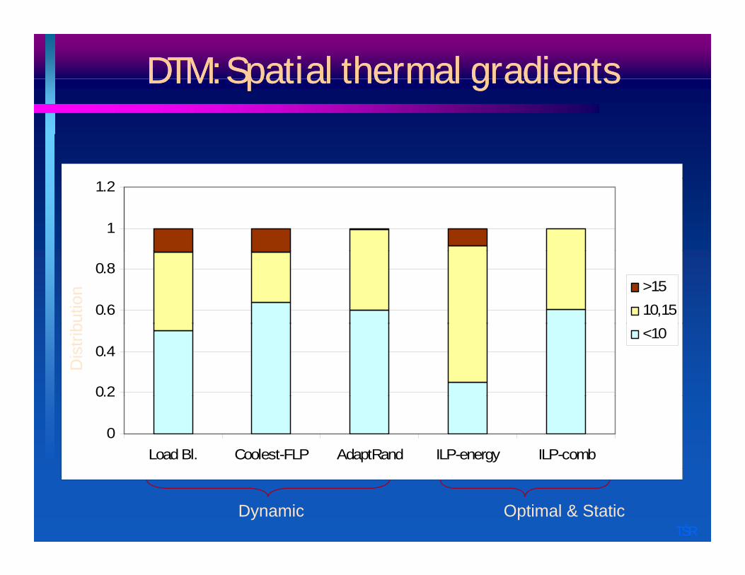
DTM: Spatial thermal gradientsDTM: Spatial thermal gradients

1

1.2

0.6

0.8>1510,15

butio

n

0.2

0.4<10

Dis

trib

0

0.2

Load Bl. Coolest-FLP AdaptRand ILP-energy ILP-comb

TŠR

Dynamic Optimal & Static

DTM: Online temperature measurementDTM: Online temperature measurement

Limited number of sensorsLimited number of sensors on a deviceSensor readings can be ginaccurate (noise, calibration, A/D quantization)

Accurate temperature estimates are often needed at the points other thanat the points other than sensor locations X Locations of Interest

1, 2 Sensor Locations

TŠR

DTM: Accurate Temperature EstimationDTM: Accurate Temperature Estimation

Offline phase (Setup) Online phase (Estimation)Offline phase (Setup) Online phase (Estimation)

Model Order Reduction

Thermal Model

Inaccurate Temperature I f ti

Inaccurate Power

E ti t

Reduced Order Thermal Model

Information Estimates

Kalman Filter Generation

Kalman FilterKalman Filter

Time UpdateMeasurement Update

Calibration

Steady State Kalman Filter

Accurate Temperature Estimates

TŠR

DTM: Results of online temperature estimationDTM: Results of online temperature estimation

Sensor MeasurementErrors (°C)

Temperature EstimationError (°C) We reduced:Errors ( C) Error ( C)

Number of Sensors

Mean Absolute

ErrorStd. Dev.

Mean Absolute

ErrorStd. Dev.

2 3 74 4 72 0 77 1 28

We reduced:Mean absolute temperature error by 5XStandard deviation of the

TŠR

2 3.74 4.72 0.77 1.28

3 3.72 4.60 0.76 1.27

4 4.41 5.50 0.75 1.27

5 3.29 3.94 0.76 1.27

Standard deviation of the error by 4X

ConclusionsConclusions

Power management can achieve large energy savings by exploiting variations in workload

TISMDP DPM/DVS policy optimized for stationary workloadsImplementable in hardware

Machine learning to optimally select among individual DPM/DVS policies

Minimizing power consumption does not always lead to optimal thermal profiles both in terms of hot spots and temperature gradientsprofiles both in terms of hot spots and temperature gradients

Thermal management:Very low overhead policies minimize hot spots and thermal gradientsDriven by sensors which can be inaccurate

Our temperature estimation uses sensor data to derive accurate

TŠR

thermal profiles online

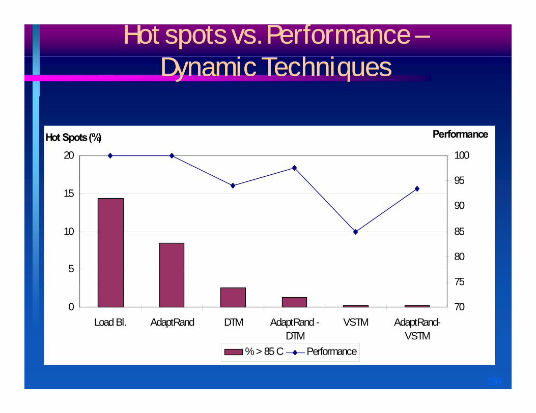
Hot spots vs. Performance –Dynamic Techniques

Hot spots vs. Performance –Dynamic Techniquesy qy q

20

Hot Spots (%)

95

100

Performance

10

15

85

90

95

5

10

75

80

85

0Load Bl. AdaptRand DTM AdaptRand -

DTMVSTM AdaptRand-

VSTM

70

75

TŠR

DTM VSTM% > 85 C Performance

DPM - Hard Disk Measurement ResultsDPM - Hard Disk Measurement Results

Policy is implemented using ACPI standard

Algorithm Power (W) Tss (s)using ACPI standard on the Hard Disk of Sony Vaio laptop running Win NT 5 0β

Oracle 0.33 118TISMDP 0.40 81Karlin's 0.44 79running Win NT 5.0β

measured real power consumption

30s Timeout 0.51 157120s Timeout 0.67 255Always on 0 95 0p

11 hr user trace

within 11% of ideal oracle policy

Always on 0.95 0Poisson 0.97 4

within 11% of ideal oracle policyfactor of 2.4 lower than always-onfactor of 1.7 lower than default time-

TŠR

out

Evaluation of experts (loss calculation)Evaluation of experts (loss calculation)

Intuition: Best suited frequency scales linearly with µ.Map task characteristics to the best suited frequency using µ-mapper.

{ 2 3 }

µ

e.g: Experts 1 to 5 = {100,200,300,400,500} MHzEvaluate experts against the best suited frequency.

0.1 0.3 0.5 0.7 0.9

0 0.2 0.6 0.80.4

µ

1.0

Expert1 µmean

Expert3 µmean

Expert4 µmean

Expert5 µmean

Expert2 µmean

TŠRwi

t+1 = wit . (1-(1-ß). lossi

t (µ)

What about Multi-tasking systems?What about Multi-tasking systems?

Tasks with different characteristics can execute togetherTasks with different characteristics can execute together.Weight vector (wt) characterizes an executing task.Need to personalize weight vector at the task level forNeed to personalize weight vector at the task level for accurate characterization.Solution: store weight vector as a task level structure

wt1 wt2 wt3 . . . wtn

TŠR

DVFS: Frequency of SelectionDVFS: Frequency of Selection

For qsortFor qsort

80low α

Higher energy

Lower Perf

50

60

70

elec

tion

medium αhigh α

energy savings

Perf Delay

30

40

quen

cy o

f Se

0

10

20Fre

TŠR

208MHz 312MHz 416MHz 520MHz