P CONVOLUTIONAL NEURAL NETWORKS FOR R EFFICIENT … · geNet (Russakovsky et al., 2015) or videos...

Published as a conference paper at ICLR 2017

PRUNING CONVOLUTIONAL NEURAL NETWORKSFOR RESOURCE EFFICIENT INFERENCE

Pavlo Molchanov, Stephen Tyree, Tero Karras, Timo Aila, Jan KautzNVIDIA{pmolchanov, styree, tkarras, taila, jkautz}@nvidia.com

ABSTRACT

We propose a new formulation for pruning convolutional kernels in neural networksto enable efficient inference. We interleave greedy criteria-based pruning with fine-tuning by backpropagation—a computationally efficient procedure that maintainsgood generalization in the pruned network. We propose a new criterion based onTaylor expansion that approximates the change in the cost function induced bypruning network parameters. We focus on transfer learning, where large pretrainednetworks are adapted to specialized tasks. The proposed criterion demonstratessuperior performance compared to other criteria, e.g. the norm of kernel weightsor feature map activation, for pruning large CNNs after adaptation to fine-grainedclassification tasks (Birds-200 and Flowers-102) relaying only on the first ordergradient information. We also show that pruning can lead to more than 10×theoretical reduction in adapted 3D-convolutional filters with a small drop inaccuracy in a recurrent gesture classifier. Finally, we show results for the large-scale ImageNet dataset to emphasize the flexibility of our approach.

1 INTRODUCTION

Convolutional neural networks (CNN) are used extensively in computer vision applications, includingobject classification and localization, pedestrian and car detection, and video classification. Manyproblems like these focus on specialized domains for which there are only small amounts of care-fully curated training data. In these cases, accuracy may be improved by fine-tuning an existingdeep network previously trained on a much larger labeled vision dataset, such as images from Ima-geNet (Russakovsky et al., 2015) or videos from Sports-1M (Karpathy et al., 2014). While transferlearning of this form supports state of the art accuracy, inference is expensive due to the time, power,and memory demanded by the heavyweight architecture of the fine-tuned network.

While modern deep CNNs are composed of a variety of layer types, runtime during prediction isdominated by the evaluation of convolutional layers. With the goal of speeding up inference, weprune entire feature maps so the resulting networks may be run efficiently even on embedded devices.We interleave greedy criteria-based pruning with fine-tuning by backpropagation, a computationallyefficient procedure that maintains good generalization in the pruned network.

Neural network pruning was pioneered in the early development of neural networks (Reed, 1993).Optimal Brain Damage (LeCun et al., 1990) and Optimal Brain Surgeon (Hassibi & Stork, 1993)leverage a second-order Taylor expansion to select parameters for deletion, using pruning as regu-larization to improve training and generalization. This method requires computation of the Hessianmatrix partially or completely, which adds memory and computation costs to standard fine-tuning.

In line with our work, Anwar et al. (2015) describe structured pruning in convolutional layers at thelevel of feature maps and kernels, as well as strided sparsity to prune with regularity within kernels.Pruning is accomplished by particle filtering wherein configurations are weighted by misclassificationrate. The method demonstrates good results on small CNNs, but larger CNNs are not addressed.

Han et al. (2015) introduce a simpler approach by fine-tuning with a strong `2 regularization termand dropping parameters with values below a predefined threshold. Such unstructured pruning is veryeffective for network compression, and this approach demonstrates good performance for intra-kernelpruning. But compression may not translate directly to faster inference since modern hardware

1

arX

iv:1

611.

0644

0v2

[cs

.LG

] 8

Jun

201

7


exploits regularities in computation for high throughput. So specialized hardware may be neededfor efficient inference of a network with intra-kernel sparsity (Han et al., 2016). This approachalso requires long fine-tuning times that may exceed the original network training by a factor of3 or larger. Group sparsity based regularization of network parameters was proposed to penalizeunimportant parameters (Wen et al., 2016; Zhou et al., 2016; Alvarez & Salzmann, 2016; Lebedev& Lempitsky, 2016). Regularization-based pruning techniques require per layer sensitivity analysiswhich adds extra computations. In contrast, our approach relies on global rescaling of criteria for alllayers and does not require sensitivity estimation. Moreover, our approach is faster as we directlyprune unimportant parameters instead of waiting for their values to be made sufficiently small byoptimization under regularization.

Other approaches include combining parameters with correlated weights (Srinivas & Babu, 2015),reducing precision (Gupta et al., 2015; Rastegari et al., 2016) or tensor decomposition (Kim et al.,2015). These approaches usually require a separate training procedure or significant fine-tuning, butpotentially may be combined with our method for additional speedups.

2 METHOD

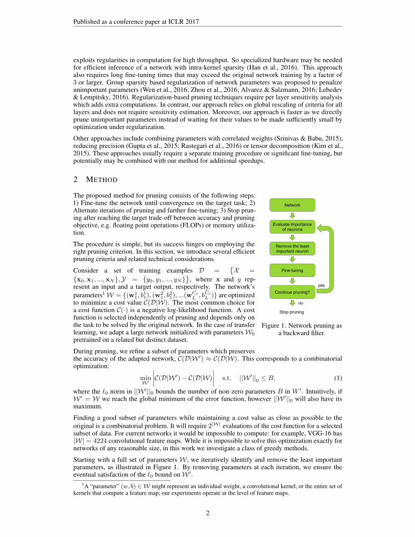
Remove the least important neuron

Fine-tuning

Evaluate importance of neurons

Continue pruning?

Network

Stop pruning

no

yes

Figure 1: Network pruning asa backward filter.

The proposed method for pruning consists of the following steps:1) Fine-tune the network until convergence on the target task; 2)Alternate iterations of pruning and further fine-tuning; 3) Stop prun-ing after reaching the target trade-off between accuracy and pruningobjective, e.g. floating point operations (FLOPs) or memory utiliza-tion.

The procedure is simple, but its success hinges on employing theright pruning criterion. In this section, we introduce several efficientpruning criteria and related technical considerations.

Consider a set of training examples D ={X =

{x0,x1, ...,xN},Y = {y0, y1, ..., yN}}

, where x and y rep-resent an input and a target output, respectively. The network’sparameters1W = {(w1

1, b11), (w2

1, b21), ...(wC`

L , bC`

L )} are optimizedto minimize a cost value C(D|W). The most common choice fora cost function C(·) is a negative log-likelihood function. A costfunction is selected independently of pruning and depends only onthe task to be solved by the original network. In the case of transferlearning, we adapt a large network initialized with parametersW0

pretrained on a related but distinct dataset.

During pruning, we refine a subset of parameters which preservesthe accuracy of the adapted network, C(D|W ′) ≈ C(D|W). This corresponds to a combinatorialoptimization:

minW′

∣∣∣∣C(D|W ′)− C(D|W)

∣∣∣∣ s.t. ||W ′||0 ≤ B, (1)

where the `0 norm in ||W ′||0 bounds the number of non-zero parameters B in W ′. Intuitively, ifW ′ = W we reach the global minimum of the error function, however ||W ′||0 will also have itsmaximum.

Finding a good subset of parameters while maintaining a cost value as close as possible to theoriginal is a combinatorial problem. It will require 2|W| evaluations of the cost function for a selectedsubset of data. For current networks it would be impossible to compute: for example, VGG-16 has|W| = 4224 convolutional feature maps. While it is impossible to solve this optimization exactly fornetworks of any reasonable size, in this work we investigate a class of greedy methods.

Starting with a full set of parameters W , we iteratively identify and remove the least importantparameters, as illustrated in Figure 1. By removing parameters at each iteration, we ensure theeventual satisfaction of the `0 bound onW ′.

1A “parameter” (w, b) ∈ W might represent an individual weight, a convolutional kernel, or the entire set ofkernels that compute a feature map; our experiments operate at the level of feature maps.

2


Since we focus our analysis on pruning feature maps from convolutional layers, let us denote aset of image feature maps by z` ∈ RH`×W`×C` with dimensionality H` ×W` and C` individualmaps (or channels).2 The feature maps can either be the input to the network, z0, or the outputfrom a convolutional layer, z` with ` ∈ [1, 2, ..., L]. Individual feature maps are denoted z

(k)` for

k ∈ [1, 2, ..., C`]. A convolutional layer ` applies the convolution operation (∗) to a set of inputfeature maps z`−1 with kernels parameterized by w

(k)` ∈ RC`−1×p×p:

z(k)` = g(k)` R

(z`−1 ∗w(k)

` + b(k)`

), (2)

where z(k)` ∈ RH`×W` is the result of convolving each ofC`−1 kernels of size p×p with its respectiveinput feature map and adding bias b(k)` . We introduce a pruning gate gl ∈ {0, 1}Cl , an external switchwhich determines if a particular feature map is included or pruned during feed-forward propagation,such that when g is vectorized: W ′ = gW .

2.1 ORACLE PRUNING

Minimizing the difference in accuracy between the full and pruned models depends on the criterion foridentifying the “least important” parameters, called saliency, at each step. The best criterion would bean exact empirical evaluation of each parameter, which we denote the oracle criterion, accomplishedby ablating each non-zero parameter w ∈ W ′ in turn and recording the cost’s difference.

We distinguish two ways of using this oracle estimation of importance: 1) oracle-loss quantifiesimportance as the signed change in loss, C(D|W ′)− C(D|W), and 2) oracle-abs adopts the absolutedifference, |C(D|W ′) − C(D|W)|. While both discourage pruning which increases the loss, theoracle-loss version encourages pruning which may decrease the loss, while oracle-abs penalizes anypruning in proportion to its change in loss, regardless of the direction of change.

While the oracle is optimal for this greedy procedure, it is prohibitively costly to compute, requiring||W ′||0 evaluations on a training dataset, one evaluation for each remaining non-zero parameter. Sinceestimation of parameter importance is key to both the accuracy and the efficiency of this pruningapproach, we propose and evaluate several criteria in terms of performance and estimation cost.

2.2 CRITERIA FOR PRUNING

There are many heuristic criteria which are much more computationally efficient than the oracle. Forthe specific case of evaluating the importance of a feature map (and implicitly the set of convolutionalkernels from which it is computed), reasonable criteria include: the combined `2-norm of thekernel weights, the mean, standard deviation or percentage of the feature map’s activation, andmutual information between activations and predictions. We describe these criteria in the followingparagraphs and propose a new criterion which is based on the Taylor expansion.

Minimum weight. Pruning by magnitude of kernel weights is perhaps the simplest possible crite-rion, and it does not require any additional computation during the fine-tuning process. In case of prun-ing according to the norm of a set of weights, the criterion is evaluated as: ΘMW : RC`−1×p×p → R,with ΘMW (w) = 1

|w|∑i w

2i , where |w| is dimensionality of the set of weights after vectorization.

The motivation to apply this type of pruning is that a convolutional kernel with low `2 norm detectsless important features than those with a high norm. This can be aided during training by applying `1or `2 regularization, which will push unimportant kernels to have smaller values.

Activation. One of the reasons for the popularity of the ReLU activation is the sparsity in activationthat is induced, allowing convolutional layers to act as feature detectors. Therefore it is reasonableto assume that if an activation value (an output feature map) is small then this feature detectoris not important for prediction task at hand. We may evaluate this by mean activation, ΘMA :

RHl×W`×C` → R, with ΘMA(a) = 1|a|∑i ai for activation a = z

(k)l , or by the standard deviation

of the activation, ΘMA_std(a) =√

1|a|∑i(ai − µa)2.

2While our notation is at times specific to 2D convolutions, the methods are applicable to 3D convolutions,as well as fully connected layers.

3


Mutual information. Mutual information (MI) is a measure of how much information is present inone variable about another variable. We apply MI as a criterion for pruning, ΘMI : RHl×W`×C` → R,with ΘMI(a) = MI(a, y), where y is the target of neural network. MI is defined for continuousvariables, so to simplify computation, we exchange it with information gain (IG), which is definedfor quantized variables IG(y|x) = H(x) +H(y)−H(x, y), where H(x) is the entropy of variablex. We accumulate statistics on activations and ground truth for a number of updates, then quantizethe values and compute IG.

Taylor expansion. We phrase pruning as an optimization problem, trying to findW ′ with boundednumber of non-zero elements that minimize

∣∣∆C(hi)∣∣ = |C(D|W ′)− C(D|W)|. With this approach

based on the Taylor expansion, we directly approximate change in the loss function from removing aparticular parameter. Let hi be the output produced from parameter i. In the case of feature maps,h = {z(1)0 , z

(2)0 , ..., z

(C`)L }. For notational convenience, we consider the cost function equally depen-

dent on parameters and outputs computed from parameters: C(D|hi) = C(D|(w, b)i). Assumingindependence of parameters, we have:∣∣∆C(hi)∣∣ =

∣∣C(D, hi = 0)− C(D, hi)∣∣, (3)

where C(D, hi = 0) is a cost value if output hi is pruned, while C(D, hi) is the cost if it is not pruned.While parameters are in reality inter-dependent, we already make an independence assumption ateach gradient step during training.

To approximate ∆C(hi), we use the first-degree Taylor polynomial. For a function f(x), the Taylorexpansion at point x = a is

f(x) =

P∑p=0

f (p)(a)

p!(x− a)p +Rp(x), (4)

where f (p)(a) is the p-th derivative of f evaluated at point a, and Rp(x) is the p-th order remainder.Approximating C(D, hi = 0) with a first-order Taylor polynomial near hi = 0, we have:

C(D, hi = 0) = C(D, hi)−δCδhi

hi +R1(hi = 0). (5)

The remainder R1(hi = 0) can be calculated through the Lagrange form:

R1(hi = 0) =δ2C

δ(h2i = ξ)

h2i2, (6)

where ξ is a real number between 0 and hi. However, we neglect this first-order remainder, largelydue to the significant calculation required, but also in part because the widely-used ReLU activationfunction encourages a smaller second order term.

Finally, by substituting Eq. (5) into Eq. (3) and ignoring the remainder, we have ΘTE :RHl×Wl×Cl → R+, with

ΘTE(hi) =∣∣∆C(hi)∣∣ =

∣∣C(D, hi)− δCδhi

hi − C(D, hi)∣∣ =

∣∣∣∣ δCδhihi∣∣∣∣. (7)

Intuitively, this criterion prunes parameters that have an almost flat gradient of the cost function w.r.t.feature map hi. This approach requires accumulation of the product of the activation and the gradientof the cost function w.r.t. to the activation, which is easily computed from the same computations forback-propagation. ΘTE is computed for a multi-variate output, such as a feature map, by

ΘTE(z(k)l ) =

∣∣∣∣ 1

M

∑m

δC

δz(k)l,m

z(k)l,m

∣∣∣∣, (8)

where M is length of vectorized feature map. For a minibatch with T > 1 examples, the criterion iscomputed for each example separately and averaged over T .

Independently of our work, Figurnov et al. (2016) came up with similar metric based on the Taylorexpansion, called impact, to evaluate importance of spatial cells in a convolutional layer. It showsthat the same metric can be applied to evaluate importance of different groups of parameters.

4


Relation to Optimal Brain Damage. The Taylor criterion proposed above relies on approximatingthe change in loss caused by removing a feature map. The core idea is the same as in Optimal BrainDamage (OBD) (LeCun et al., 1990). Here we consider the differences more carefully.

The primary difference is the treatment of the first-order term of the Taylor expansion, in our notationy = δC

δhh for cost function C and hidden layer activation h. After sufficient training epochs, thegradient term tends to zero: δCδh → 0 and E(y) = 0. At face value y offers little useful information,hence OBD regards the term as zero and focuses on the second-order term.

However, the variance of y is non-zero and correlates with the stability of the local function w.r.t.activation h. By considering the absolute change in the cost3 induced by pruning (as in Eq. 3), we usethe absolute value of the first-order term, |y|. Under assumption that samples come from independentand identical distribution, E(|y|) = σ

√2/√π where σ is the standard deviation of y, known as the

expected value of the half-normal distribution. So, while y tends to zero, the expectation of |y| isproportional to the variance of y, a value which is empirically more informative as a pruning criterion.

As an additional benefit, we avoid the computation of the second-order Taylor expansion term, or itssimplification - diagonal of the Hessian, as required in OBD.

We found important to compare proposed Taylor criteria to OBD. As described in the originalpapers (LeCun et al., 1990; 1998), OBD can be efficiently implemented similarly to standard backpropagation algorithm doubling backward propagation time and memory usage when used togetherwith standard fine-tuning. Efficient implementation of the original OBD algorithm might requiresignificant changes to the framework based on automatic differentiation like Theano to efficientlycompute only diagonal of the Hessian instead of the full matrix. Several researchers tried to tackle thisproblem with approximation techniques (Martens, 2010; Martens et al., 2012). In our implementation,we use efficient way of computing Hessian-vector product (Pearlmutter, 1994) and matrix diagonalapproximation proposed by (Bekas et al., 2007), please refer to more details in appendix. Withcurrent implementation, OBD is 30 times slower than Taylor technique for saliency estimation, and 3times slower for iterative pruning, however with different implementation can only be 50% slower asmentioned in the original paper.

Average Percentage of Zeros (APoZ). Hu et al. (2016) proposed to explore sparsity in activationsfor network pruning. ReLU activation function imposes sparsity during inference, and averagepercentage of positive activations at the output can determine importance of the neuron. Intuitively,it is a good criteria, however feature maps at the first layers have similar APoZ regardless of thenetwork’s target as they learn to be Gabor like filters. We will use APoZ to estimate saliency offeature maps.

2.3 NORMALIZATION

Some criteria return “raw” values, whose scale varies with the depth of the parameter’s layer in thenetwork. A simple layer-wise `2-normalization can achieve adequate rescaling across layers:

Θ̂(z(k)l )=

Θ(z(k)l )√∑

j

(Θ(z

(j)l ))2 .

2.4 FLOPS REGULARIZED PRUNING

One of the main reasons to apply pruning is to reduce number of operations in the network. Featuremaps from different layers require different amounts of computation due the number and sizes of inputfeature maps and convolution kernels. To take this into account we introduce FLOPs regularization:

Θ(z(k)l ) = Θ(z

(k)l )− λΘflops

l , (9)

where λ controls the amount of regularization. For our experiments, we use λ = 10−3. Θflops iscomputed under the assumption that convolution is implemented as a sliding window (see Appendix).Other regularization conditions may be applied, e.g. storage size, kernel sizes, or memory footprint.

3OBD approximates the signed difference in loss, while our method approximates absolute difference in loss.We find in our results that pruning based on absolute difference yields better accuracy.

5


Figure 2: Global statistics of oracle ranking,shown by layer for Birds-200 transfer learning.

Figure 3: Pruning without fine-tuning usingoracle ranking for Birds-200 transfer learning.

3 RESULTS

We empirically study the pruning criteria and procedure detailed in the previous section for a variety ofproblems. We focus many experiments on transfer learning problems, a setting where pruning seemsto excel. We also present results for pruning large networks on their original tasks for more directcomparison with the existing pruning literature. Experiments are performed within Theano (TheanoDevelopment Team, 2016). Training and pruning are performed on the respective training sets foreach problem, while results are reported on appropriate holdout sets, unless otherwise indicated. Forall experiments we prune a single feature map at every pruning iteration, allowing fine-tuning andre-evaluation of the criterion to account for dependency between parameters.

3.1 CHARACTERIZING THE ORACLE RANKING

We begin by explicitly computing the oracle for a single pruning iteration of a visual transfer learningproblem. We fine-tune the VGG-16 network (Simonyan & Zisserman, 2014) for classification of birdspecies using the Caltech-UCSD Birds 200-2011 dataset (Wah et al., 2011). The dataset consists ofnearly 6000 training images and 5700 test images, covering 200 species. We fine-tune VGG-16 for60 epochs with learning rate 0.0001 to achieve a test accuracy of 72.2% using uncropped images.

To compute the oracle, we evaluate the change in loss caused by removing each individual featuremap from the fine-tuned VGG-16 network. (See Appendix A.3 for additional analysis.) We rankfeature maps by their contributions to the loss, where rank 1 indicates the most important featuremap—removing it results in the highest increase in loss—and rank 4224 indicates the least important.Statistics of global ranks are shown in Fig. 2 grouped by convolutional layer. We observe: (1)Median global importance tends to decrease with depth. (2) Layers with max-pooling tend to bemore important than those without. (VGG-16 has pooling after layers 2, 4, 7, 10, and 13.) However,(3) maximum and minimum ranks show that every layer has some feature maps that are globallyimportant and others that are globally less important. Taken together with the results of subsequentexperiments, we opt for encouraging a balanced pruning that distributes selection across all layers.

Next, we iteratively prune the network using pre-computed oracle ranking. In this experiment, we donot update the parameters of the network or the oracle ranking between iterations. Training accuracyis illustrated in Fig. 3 over many pruning iterations. Surprisingly, pruning by smallest absolutechange in loss (Oracle-abs) yields higher accuracy than pruning by the net effect on loss (Oracle-loss).Even though the oracle indicates that removing some feature maps individually may decrease loss,instability accumulates due the large absolute changes that are induced. These results support pruningby absolute difference in cost, as constructed in Eq. 1.

3.2 EVALUATING PROPOSED CRITERIA VERSUS THE ORACLE

To evaluate computationally efficient criteria as substitutes for the oracle, we compute Spearman’srank correlation, an estimate of how well two predictors provide monotonically related outputs,

6


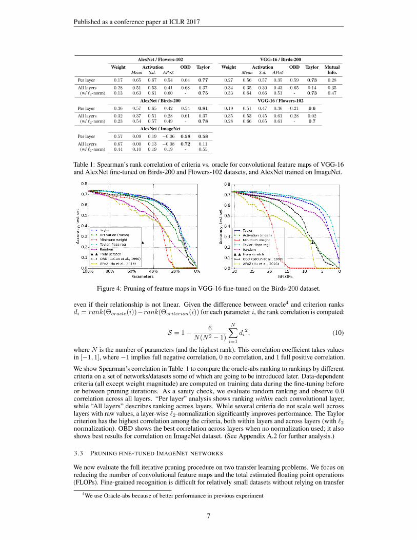
AlexNet / Flowers-102 VGG-16 / Birds-200Weight Activation OBD Taylor Weight Activation OBD Taylor Mutual

Mean S.d. APoZ Mean S.d. APoZ Info.Per layer 0.17 0.65 0.67 0.54 0.64 0.77 0.27 0.56 0.57 0.35 0.59 0.73 0.28

All layers 0.28 0.51 0.53 0.41 0.68 0.37 0.34 0.35 0.30 0.43 0.65 0.14 0.35(w/ `2-norm) 0.13 0.63 0.61 0.60 - 0.75 0.33 0.64 0.66 0.51 - 0.73 0.47

AlexNet / Birds-200 VGG-16 / Flowers-102Per layer 0.36 0.57 0.65 0.42 0.54 0.81 0.19 0.51 0.47 0.36 0.21 0.6

All layers 0.32 0.37 0.51 0.28 0.61 0.37 0.35 0.53 0.45 0.61 0.28 0.02(w/ `2-norm) 0.23 0.54 0.57 0.49 - 0.78 0.28 0.66 0.65 0.61 - 0.7

AlexNet / ImageNetPer layer 0.57 0.09 0.19 −0.06 0.58 0.58

All layers 0.67 0.00 0.13 −0.08 0.72 0.11(w/ `2-norm) 0.44 0.10 0.19 0.19 - 0.55

Table 1: Spearman’s rank correlation of criteria vs. oracle for convolutional feature maps of VGG-16and AlexNet fine-tuned on Birds-200 and Flowers-102 datasets, and AlexNet trained on ImageNet.

Figure 4: Pruning of feature maps in VGG-16 fine-tuned on the Birds-200 dataset.

even if their relationship is not linear. Given the difference between oracle4 and criterion ranksdi = rank(Θoracle(i))−rank(Θcriterion(i)) for each parameter i, the rank correlation is computed:

S = 1− 6

N(N2 − 1)

N∑i=1

di2, (10)

where N is the number of parameters (and the highest rank). This correlation coefficient takes valuesin [−1, 1], where −1 implies full negative correlation, 0 no correlation, and 1 full positive correlation.

We show Spearman’s correlation in Table 1 to compare the oracle-abs ranking to rankings by differentcriteria on a set of networks/datasets some of which are going to be introduced later. Data-dependentcriteria (all except weight magnitude) are computed on training data during the fine-tuning beforeor between pruning iterations. As a sanity check, we evaluate random ranking and observe 0.0correlation across all layers. “Per layer” analysis shows ranking within each convolutional layer,while “All layers” describes ranking across layers. While several criteria do not scale well acrosslayers with raw values, a layer-wise `2-normalization significantly improves performance. The Taylorcriterion has the highest correlation among the criteria, both within layers and across layers (with `2normalization). OBD shows the best correlation across layers when no normalization used; it alsoshows best results for correlation on ImageNet dataset. (See Appendix A.2 for further analysis.)

3.3 PRUNING FINE-TUNED IMAGENET NETWORKS

We now evaluate the full iterative pruning procedure on two transfer learning problems. We focus onreducing the number of convolutional feature maps and the total estimated floating point operations(FLOPs). Fine-grained recognition is difficult for relatively small datasets without relying on transfer

4We use Oracle-abs because of better performance in previous experiment

7


Figure 5: Pruning of feature maps in AlexNet on fine-tuned on Flowers-102.

learning. Branson et al. (2014) show that training CNN from scratch on the Birds-200 dataset achievestest accuracy of only 10.9%. We compare results to training a randomly initialized CNN with halfthe number of parameters per layer, denoted "from scratch".

Fig. 4 shows pruning of VGG-16 after fine-tuning on the Birds-200 dataset (as described previously).At each pruning iteration, we remove a single feature map and then perform 30 minibatch SGDupdates with batch-size 32, momentum 0.9, learning rate 10−4, and weight decay 10−4. The figuredepicts accuracy relative to the pruning rate (left) and estimated GFLOPs (right). The Taylor criterionshows the highest accuracy for nearly the entire range of pruning ratios, and with FLOPs regularizationdemonstrates the best performance relative to the number of operations. OBD shows slightly worseperformance of pruning in terms of parameters, however significantly worse in terms of FLOPs.

In Fig. 5, we show pruning of the CaffeNet implementation of AlexNet (Krizhevsky et al., 2012) afteradapting to the Oxford Flowers 102 dataset (Nilsback & Zisserman, 2008), with 2040 training and6129 test images from 102 species of flowers. Criteria correlation with oracle-abs is summarized inTable 1. We initially fine-tune the network for 20 epochs using a learning rate of 0.001, achieving afinal test accuracy of 80.1%. Then pruning procedes as previously described for Birds-200, exceptwith only 10 mini-batch updates between pruning iterations. We observe the superior performance ofthe Taylor and OBD criteria in both number of parameters and GFLOPs.

We observed that Taylor criterion shows the best performance which is closely followed by OBD witha bit lower Spearman’s rank correlation coefficient. Implementing OBD takes more effort because ofcomputation of diagonal of the Hessian and it is 50% to 300% slower than Taylor criteria that relieson first order gradient only.

Fig. 6 shows pruning with the Taylor technique and a varying number of fine-tuning updates betweenpruning iterations. Increasing the number of updates results in higher accuracy, but at the cost ofadditional runtime of the pruning procedure.

During pruning we observe a small drop in accuracy. One of the reasons is fine-tuning betweenpruning iterations. Accuracy of the initial network can be improved with longer fine tunning andsearch of better optimization parameters. For example accuracy of unpruned VGG16 network onBirds-200 goes up to 75% after extra 128k updates. And AlexNet on Flowers-102 goes up to 82.9%after 130k updates. It should be noted that with farther fine-tuning of pruned networks we can achievehigher accuracy as well, therefore the one-to-one comparison of accuracies is rough.

3.4 PRUNING A RECURRENT 3D-CNN NETWORK FOR HAND GESTURE RECOGNITION

Molchanov et al. (2016) learn to recognize 25 dynamic hand gestures in streaming video with a largerecurrent neural network. The network is constructed by adding recurrent connections to a 3D-CNNpretrained on the Sports-1M video dataset (Karpathy et al., 2014) and fine tuning on a gesture dataset.The full network achieves an accuracy of 80.7% when trained on the depth modality, but a singleinference requires an estimated 37.8 GFLOPs, too much for deployment on an embedded GPU. Afterseveral iterations of pruning with the Taylor criterion with learning rate 0.0003, momentum 0.9,FLOPs regularization 10−3, we reduce inference to 3.0 GFLOPs, as shown in Fig. 7. While pruning

8


Figure 6: Varying the number of minibatchupdates between pruning iterations with

AlexNet/Flowers-102 and the Taylor criterion.

Figure 7: Pruning of a recurrent 3D-CNN fordynamic hand gesture recognition

(Molchanov et al., 2016).

Figure 8: Pruning of AlexNet on Imagenet with varying number of updates between pruning iterations.

increases classification error by nearly 6%, additional fine-tuning restores much of the lost accuracy,yielding a final pruned network with a 12.6× reduction in GFLOPs and only a 2.5% loss in accuracy.

3.5 PRUNING NETWORKS FOR IMAGENET

Figure 9: Pruning of the VGG-16 network onImageNet, with additional following fine-tuning at

11.5 and 8 GFLOPs.

We also test our pruning scheme on the large-scale ImageNet classification task. In the firstexperiment, we begin with a trained CaffeNetimplementation of AlexNet with 79.2% top-5validation accuracy. Between pruning iterations,we fine-tune with learning rate 10−4, momen-tum 0.9, weight decay 10−4, batch size 32, anddrop-out 50%. Using a subset of 5000 trainingimages, we compute oracle-abs and Spearman’srank correlation with the criteria, as shown inTable 1. Pruning traces are illustrated in Fig. 8.

We observe: 1) Taylor performs better than ran-dom or minimum weight pruning when 100 up-dates are used between pruning iterations. Whenresults are displayed w.r.t. FLOPs, the differ-ence with random pruning is only 0%−4%, butthe difference is higher, 1%−10%, when plot-ted with the number of feature maps pruned. 2)Increasing the number of updates from 100 to1000 improves performance of pruning signifi-cantly for both the Taylor criterion and randompruning.

9


Hardware Batch Accuracy Time, ms Accuracy Time (speed up) Accuracy Time (speed up)AlexNet / Flowers-102, 1.46 GFLOPs 41% feature maps, 0.4 GFLOPs 19.5% feature maps, 0.2 GFLOPsCPU: Intel Core i7-5930K 16 80.1% 226.4 79.8%(-0.3%) 121.4 (1.9x) 74.1%(-6.0%) 87.0 (2.6x)GPU: GeForce GTX TITAN X (Pascal) 16 4.8 2.4 (2.0x) 1.9 (2.5x)GPU: GeForce GTX TITAN X (Pascal) 512 88.3 36.6 (2.4x) 27.4 (3.2x)GPU: NVIDIA Jetson TX1 32 169.2 73.6 (2.3x) 58.6 (2.9x)

VGG-16 / ImageNet, 30.96 GFLOPs 66% feature maps, 11.5 GFLOPs 52% feature maps, 8.0 GFLOPsCPU: Intel Core i7-5930K 16 89.3% 2564.7 87.0% (-2.3%) 1483.3 (1.7x) 84.5% (-4.8%) 1218.4 (2.1x)GPU: GeForce GTX TITAN X (Pascal) 16 68.3 31.0 (2.2x) 20.2 (3.4x)GPU: NVIDIA Jetson TX1 4 456.6 182.5 (2.5x) 138.2 (3.3x)

R3DCNN / nvGesture, 37.8 GFLOPs 25% feature maps, 3 GFLOPsGPU: GeForce GT 730M 1 80.7% 438.0 78.2% (-2.5%) 85.0 (5.2x)

Table 2: Actual speed up of networks pruned by Taylor criterion for various hardware setup. Allmeasurements were performed with PyTorch with cuDNN v5.1.0, except R3DCNN which wasimplemented in C++ with cuDNN v4.0.4). Results for ImageNet dataset are reported as top-5accuracy on validation set. Results on AlexNet / Flowers-102 are reported for pruning with 1000updates between iterations and no fine-tuning after pruning.

For a second experiment, we prune a trained VGG-16 network with the same parameters as before,except enabling FLOPs regularization. We stop pruning at two points, 11.5 and 8.0 GFLOPs, andfine-tune both models for an additional five epochs with learning rate 10−4. Fine-tuning after pruningsignificantly improves results: the network pruned to 11.5 GFLOPs improves from 83% to 87% top-5validation accuracy, and the network pruned to 8.0 GFLOPs improves from 77.8% to 84.5%.

3.6 SPEED UP MEASUREMENTS

During pruning we were measuring reduction in computations by FLOPs, which is a common practice(Han et al., 2015; Lavin, 2015a;b). Improvements in FLOPs result in monotonically decreasinginference time of the networks because of removing entire feature map from the layer. However,time consumed by inference dependents on particular implementation of convolution operator,parallelization algorithm, hardware, scheduling, memory transfer rate etc. Therefore we measureimprovement in the inference time for selected networks to see real speed up compared to unprunednetworks in Table 2. We observe significant speed ups by proposed pruning scheme.

4 CONCLUSIONS

We propose a new scheme for iteratively pruning deep convolutional neural networks. We find: 1)CNNs may be successfully pruned by iteratively removing the least important parameters—featuremaps in this case—according to heuristic selection criteria; 2) a Taylor expansion-based criteriondemonstrates significant improvement over other criteria; 3) per-layer normalization of the criterionis important to obtain global scaling.

REFERENCES

Jose M Alvarez and Mathieu Salzmann. Learning the Number of Neurons in Deep Networks. InD. D. Lee, M. Sugiyama, U. V. Luxburg, I. Guyon, and R. Garnett (eds.), Advances in NeuralInformation Processing Systems 29, pp. 2262–2270. Curran Associates, Inc., 2016.

Sajid Anwar, Kyuyeon Hwang, and Wonyong Sung. Structured pruning of deep convolutional neuralnetworks. arXiv preprint arXiv:1512.08571, 2015. URL http://arxiv.org/abs/1512.08571.

Costas Bekas, Effrosyni Kokiopoulou, and Yousef Saad. An estimator for the diagonal of a matrix.Applied numerical mathematics, 57(11):1214–1229, 2007.

Steve Branson, Grant Van Horn, Serge Belongie, and Pietro Perona. Bird species categorization usingpose normalized deep convolutional nets. arXiv preprint arXiv:1406.2952, 2014.

Yann Dauphin, Harm de Vries, and Yoshua Bengio. Equilibrated adaptive learning rates for non-convex optimization. In Advances in Neural Information Processing Systems, pp. 1504–1512,2015.

10

http://arxiv.org/abs/1512.08571



Mikhail Figurnov, Aizhan Ibraimova, Dmitry P Vetrov, and Pushmeet Kohli. PerforatedCNNs:Acceleration through elimination of redundant convolutions. In Advances in Neural InformationProcessing Systems, pp. 947–955, 2016.

Suyog Gupta, Ankur Agrawal, Kailash Gopalakrishnan, and Pritish Narayanan. Deep learning withlimited numerical precision. CoRR, abs/1502.02551, 392, 2015. URL http://arxiv.org/abs/1502.025513.

Song Han, Jeff Pool, John Tran, and William Dally. Learning both weights and connections forefficient neural network. In Advances in Neural Information Processing Systems, pp. 1135–1143,2015.

Song Han, Xingyu Liu, Huizi Mao, Jing Pu, Ardavan Pedram, Mark A. Horowitz, and William J.Dally. EIE: Efficient inference engine on compressed deep neural network. In Proceedings of the43rd International Symposium on Computer Architecture, ISCA ’16, pp. 243–254, Piscataway, NJ,USA, 2016. IEEE Press.

Babak Hassibi and David G. Stork. Second order derivatives for network pruning: Optimal brainsurgeon. In Advances in Neural Information Processing Systems (NIPS), pp. 164–171, 1993.

Hengyuan Hu, Rui Peng, Yu-Wing Tai, and Chi-Keung Tang. Network trimming: A data-drivenneuron pruning approach towards efficient deep architectures. arXiv preprint arXiv:1607.03250,2016.

Andrej Karpathy, George Toderici, Sanketh Shetty, Thomas Leung, Rahul Sukthankar, and Li Fei-Fei.Large-scale video classification with convolutional neural networks. In CVPR, 2014.

Yong-Deok Kim, Eunhyeok Park, Sungjoo Yoo, Taelim Choi, Lu Yang, and Dongjun Shin. Com-pression of deep convolutional neural networks for fast and low power mobile applications. InProceedings of the International Conference on Learning Representations (ICLR), 2015.

Alex Krizhevsky, Ilya Sutskever, and Geoffrey E Hinton. Imagenet classification with deep convolu-tional neural networks. In Advances in neural information processing systems, pp. 1097–1105,2012.

Andrew Lavin. maxDNN: An Efficient Convolution Kernel for Deep Learning with Maxwell GPUs.CoRR, abs/1501.06633, 2015a. URL http://arxiv.org/abs/1501.06633.

Andrew Lavin. Fast algorithms for convolutional neural networks. arXiv preprint arXiv:1509.09308,2015b.

Vadim Lebedev and Victor Lempitsky. Fast convnets using group-wise brain damage. In Proceedingsof the IEEE Conference on Computer Vision and Pattern Recognition, pp. 2554–2564, 2016.

Yann LeCun, J. S. Denker, S. Solla, R. E. Howard, and L. D. Jackel. Optimal brain damage. InAdvances in Neural Information Processing Systems (NIPS), 1990.

Yann LeCun, Leon Bottou, Genevieve B. Orr, and Klaus Robert Müller. Efficient BackProp, pp. 9–50.Springer Berlin Heidelberg, Berlin, Heidelberg, 1998.

James Martens. Deep learning via Hessian-free optimization. In Proceedings of the 27th InternationalConference on Machine Learning (ICML-10), pp. 735–742, 2010.

James Martens, Ilya Sutskever, and Kevin Swersky. Estimating the Hessian by back-propagatingcurvature. arXiv preprint arXiv:1206.6464, 2012.

Pavlo Molchanov, Xiaodong Yang, Shalini Gupta, Kihwan Kim, Stephen Tyree, and Jan Kautz.Online detection and classification of dynamic hand gestures with recurrent 3d convolutionalneural network. In The IEEE Conference on Computer Vision and Pattern Recognition (CVPR),June 2016.

M-E. Nilsback and A. Zisserman. Automated flower classification over a large number of classes. InProceedings of the Indian Conference on Computer Vision, Graphics and Image Processing, Dec2008.

11





Barak A. Pearlmutter. Fast Exact Multiplication by the Hessian. Neural Computation, 6:147–160,1994.

Mohammad Rastegari, Vicente Ordonez, Joseph Redmon, and Ali Farhadi. XNOR-Net: ImageNetClassification Using Binary Convolutional Neural Networks. CoRR, abs/1603.05279, 2016. URLhttp://arxiv.org/abs/1603.05279.

Russell Reed. Pruning algorithms-a survey. IEEE transactions on Neural Networks, 4(5):740–747,1993.

Olga Russakovsky, Jia Deng, Hao Su, Jonathan Krause, Sanjeev Satheesh, Sean Ma, Zhiheng Huang,Andrej Karpathy, Aditya Khosla, Michael Bernstein, Alexander C. Berg, and Li Fei-Fei. ImageNetLarge Scale Visual Recognition Challenge. International Journal of Computer Vision (IJCV), 115(3):211–252, 2015.

K. Simonyan and A. Zisserman. Very deep convolutional networks for large-scale image recognition.CoRR, abs/1409.1556, 2014.

Suraj Srinivas and R. Venkatesh Babu. Data-free parameter pruning for deep neural networks. InMark W. Jones Xianghua Xie and Gary K. L. Tam (eds.), Proceedings of the British MachineVision Conference (BMVC), pp. 31.1–31.12. BMVA Press, September 2015.

Theano Development Team. Theano: A Python framework for fast computation of mathematicalexpressions. arXiv e-prints, abs/1605.02688, May 2016. URL http://arxiv.org/abs/1605.02688.

Catherine Wah, Steve Branson, Peter Welinder, Pietro Perona, and Serge Belongie. The caltech-ucsdbirds-200-2011 dataset. 2011.

Wei Wen, Chunpeng Wu, Yandan Wang, Yiran Chen, and Hai Li. Learning structured sparsity indeep neural networks. In Advances in Neural Information Processing Systems, pp. 2074–2082,2016.

Hao Zhou, Jose M. Alvarez, and Fatih Porikli. Less is more: Towards compact cnns. In EuropeanConference on Computer Vision, pp. 662–677, Amsterdam, the Netherlands, October 2016.

12





A APPENDIX

A.1 FLOPS COMPUTATION

To compute the number of floating-point operations (FLOPs), we assume convolution is implementedas a sliding window and that the nonlinearity function is computed for free. For convolutional kernelswe have:

FLOPs = 2HW (CinK2 + 1)Cout, (11)

where H , W and Cin are height, width and number of channels of the input feature map, K is thekernel width (assumed to be symmetric), and Cout is the number of output channels.

For fully connected layers we compute FLOPs as:

FLOPs = (2I − 1)O, (12)

where I is the input dimensionality and O is the output dimensionality.

We apply FLOPs regularization during pruning to prune neurons with higher FLOPs first. FLOPs perconvolutional neuron in every layer:

VGG16: Θflops = [3.1, 57.8, 14.1, 28.9, 7.0, 14.5, 14.5, 3.5, 7.2, 7.2, 1.8, 1.8, 1.8, 1.8]

AlexNet: Θflops = [2.3, 1.7, 0.8, 0.6, 0.6]

R3DCNN: Θflops = [5.6, 86.9, 21.7, 43.4, 5.4, 10.8, 1.4, 1.4]

A.2 NORMALIZATION ACROSS LAYERS

Scaling a criterion across layers is very important for pruning. If the criterion is not properly scaled,then a hand-tuned multiplier would need to be selected for each layer. Statistics of feature mapranking by different criteria are shown in Fig. 10. Without normalization (Fig. 14a–14d), the weightmagnitude criterion tends to rank feature maps from the first layers more important than last layers;the activation criterion ranks middle layers more important; and Taylor ranks first layers higher. After`2 normalization (Fig. 10d–10f), all criteria have a shape more similar to the oracle, where each layerhas some feature maps which are highly important and others which are unimportant.

(a) Weight (b) Activation (mean) (c) Taylor

(d) Weight + `2 (e) Activation (mean) + `2 (f) Taylor + `2

Figure 10: Statistics of feature map ranking by raw criteria values (top) and by criteria values after `2normalization (bottom).

13


MI Weight Activation OBD TaylorMean S.d. APoZ

Per layerLayer 1 0.41 0.40 0.65 0.78 0.36 0.54 0.95Layer 2 0.23 0.57 0.56 0.59 0.33 0.78 0.90Layer 3 0.14 0.55 0.48 0.45 0.51 0.66 0.74Layer 4 0.26 0.23 0.58 0.42 0.10 0.36 0.80Layer 5 0.17 0.28 0.49 0.52 0.15 0.54 0.69Layer 6 0.21 0.18 0.41 0.48 0.16 0.49 0.63Layer 7 0.12 0.19 0.54 0.49 0.38 0.55 0.71Layer 8 0.18 0.23 0.43 0.42 0.30 0.50 0.54Layer 9 0.21 0.18 0.50 0.55 0.35 0.53 0.61Layer 10 0.26 0.15 0.59 0.60 0.45 0.61 0.66Layer 11 0.41 0.12 0.61 0.65 0.45 0.64 0.72Layer 12 0.47 0.15 0.60 0.66 0.39 0.66 0.72Layer 13 0.61 0.21 0.77 0.76 0.65 0.76 0.77Mean 0.28 0.27 0.56 0.57 0.35 0.59 0.73

All layersNo normalization 0.35 0.34 0.35 0.30 0.43 0.65 0.14`1 normalization 0.47 0.37 0.63 0.63 0.52 0.65 0.71`2 normalization 0.47 0.33 0.64 0.66 0.51 0.60 0.73Min-max normalization 0.27 0.17 0.52 0.57 0.42 0.54 0.67

Table 3: Spearman’s rank correlation of criteria vs oracle-abs in VGG-16 fine-tuned on Birds 200.

A.3 ORACLE COMPUTATION FOR VGG-16 ON BIRDS-200

We compute the change in the loss caused by removing individual feature maps from the VGG-16network, after fine-tuning on the Birds-200 dataset. Results are illustrated in Fig. 11a-11b for eachfeature map in layers 1 and 13, respectively. To compute the oracle estimate for a feature map, weremove the feature map and compute the network prediction for each image in the training set usingthe central crop with no data augmentation or dropout. We draw the following conclusions:

• The contribution of feature maps range from positive (above the red line) to slightly negative(below the red line), implying the existence of some feature maps which decrease the trainingcost when removed.

• There are many feature maps with little contribution to the network output, indicated byalmost zero change in loss when removed.

• Both layers contain a small number of feature maps which induce a significant increase inthe loss when removed.

(a) Layer 1 (b) Layer 13

Figure 11: Change in training loss as a function of the removal of a single feature map from theVGG-16 network after fine-tuning on Birds-200. Results are plotted for two convolutional layers w.r.t.the index of the removed feature map index. The loss with all feature maps, 0.00461, is indicatedwith a red horizontal line.

14


Figure 12: Comparison of our iterative pruning with pruning by regularization

Table 3 contains a layer-by-layer listing of Spearman’s rank correlation of several criteria with theranking of oracle-abs. In this more detailed comparison, we see the Taylor criterion shows highercorrelation for all individual layers. For several methods including Taylor, the worst correlationsare observed for the middle of the network, layers 5-10. We also evaluate several techniques fornormalization of the raw criteria values for comparison across layers. The table shows the bestperformance is obtained by `2 normalization, hence we select it for our method.

A.4 COMPARISON WITH WEIGHT REGULARIZATION

Han et al. (2015) find that fine-tuning with high `1 or `2 regularization causes unimportant connectionsto be suppressed. Connections with energy lower than some threshold can be removed on theassumption that they do not contribute much to subsequent layers. The same work also finds thatthresholds must be set separately for each layer depending on its sensitivity to pruning. The procedureto evaluate sensitivity is time-consuming as it requires pruning layers independently during evaluation.

The idea of pruning with high regularization can be extended to removing the kernels for an entirefeature map if the `2 norm of those kernels is below a predefined threshold. We compare our approachwith this regularization-based pruning for the task of pruning the last convolutional layer of VGG-16fine-tuned for Birds-200. By considering only a single layer, we avoid the need to compute layerwisesensitivity. Parameters for optimization during fine-tuning are the same as other experiments with theBirds-200 dataset. For the regularization technique, the pruning threshold is set to σ = 10−5 whilewe vary the regularization coefficient γ of the `2 norm on each feature map kernel.5 We prune onlykernel weights, while keeping the bias to maintain the same expected output.

A comparison between pruning based on regularization and our greedy scheme is illustrated inFig. 12. We observe that our approach has higher test accuracy for the same number of remainingunpruned feature maps, when pruning 85% or more of the feature maps. We observe that with highregularization all weights tend to zero, not only unimportant weights as Han et al. (2015) observe inthe case of ImageNet networks. The intuition here is that with regularization we push all weightsdown and potentially can affect important connections for transfer learning, whereas in our iterativeprocedure we only remove unimportant parameters leaving others untouched.

A.5 COMBINATION OF CRITERIA

One of the possibilities to improve saliency estimation is to combine several criteria together. One ofthe straight forward combinations is Taylor and mean activation of the neuron. We compute the jointcriteria as Θjoint(z

(k)l ) = (1− λ)Θ̂Taylor(z

(k)l ) + λΘ̂Activation(z

(k)l ) and perform a grid search of

parameter λ in Fig.13. The highest correlation value for each dataset is marked with with vertical barwith λ and gain. We observe that the gain of linearly combining criteria is negligibly small (see ∆’sin the figure).

5In our implementation, the regularization coefficient is multiplied by the learning rate equal to 10−4.

15


Figure 13: Spearman rank correlation for linear combination of criteria. The per layer metric is used.Each ∆ indicates the gain in correlation for one experiment.

A.6 OPTIMAL BRAIN DAMAGE IMPLEMENTATION

OBD computes saliency of a parameter by computing a product of the squared magnitude of theparameter and the corresponding element on the diagonal of the Hessian. For many deep learningframeworks, an efficient implementation of the diagonal evaluation is not straightforward andapproximation techniques must be applied. Our implementation of Hessian diagonal computationwas inspired by Dauphin et al. (2015) work, where the technique proposed by Bekas et al. (2007) wasused to evaluate SGD preconditioned with the Jacobi preconditioner. It was shown that diagonal ofthe Hessian can be approximated as:

diag(H) = E[v�Hv] = E[v�∇(∇C · v)], (13)

where � is the element-wise product, v are random vectors with entries ±1, and ∇ is the gradientoperator. To compute saliency with OBD, we randomly draw v and compute the diagonal over 10iterations for a single minibatch for 1000 mini batches. We found that this number of mini batches isrequired to compute close approximation of the Hessian’s diagonal (which we verified). Computingsaliency this way is computationally expensive for iterative pruning, and we use a slightly differentbut more efficient procedure. Before the first pruning iteration, saliency is initialized from valuescomputed off-line with 1000 minibatches and 10 iterations, as described above. Then, at everyminibatch we compute the OBD criteria with only one iteration and apply an exponential movingaveraging with a coefficient of 0.99. We verified that this computes a close approximation to theHessian’s diagonal.

A.7 CORRELATION OF TAYLOR CRITERION WITH GRADIENT AND ACTIVATION

The Taylor criterion is composed of both an activation term and a gradient term. In Figure 14, wedepict the correlation between the Taylor criterion and each constituent part. We consider expectedabsolute value of the gradient instead of the mean, because otherwise it tends to zero. The plots arecomputed from pruning criteria for an unpruned VGG network fine-tuned for the Birds-200 dataset.(Values are shown after layer-wise normalization). Figure 14(a-b) depict the Taylor criterion in they-axis for all neurons w.r.t. the gradient and activation components, respectively. The bottom 10% ofneurons (lowest Taylor criterion, most likely to be pruned) are depicted in red, while the top 10% areshown in green. Considering all neurons, both gradient and activation components demonstrate alinear trend with the Taylor criterion. However, for the bottom 10% of neurons, as shown in Figure14(c-d), the activation criterion shows much stronger correlation, with lower activations indicatinglower Taylor scores.

16


(a) (b)

(c) (d)

Figure 14: Correlation of Taylor criterion with gradient and activation (after layer-wise `2 normaliza-tion) for all neurons (a-b) and bottom 10% of neurons (c-d) for unpruned VGG after fine-tuning onBirds-200.

17

P CONVOLUTIONAL NEURAL NETWORKS FOR R EFFICIENT … · geNet (Russakovsky et al., 2015) or videos...

Documents

Transcript of P CONVOLUTIONAL NEURAL NETWORKS FOR R EFFICIENT … · geNet (Russakovsky et al., 2015) or videos...