OWNERSHIP OF STOCKS AND MUTUAL FUNDS: A PANEL DATA …
39
No. 2001-94 OWNERSHIP OF STOCKS AND MUTUAL FUNDS: A PANEL DATA ANALYSIS By Rob Alessie, Stefan Hochguertel and Arthur van Soest December 2001 ISSN 0924-7815 brought to you by CORE View metadata, citation and similar papers at core.ac.uk provided by Research Papers in Economics
Transcript of OWNERSHIP OF STOCKS AND MUTUAL FUNDS: A PANEL DATA …

No. 2001-94
OWNERSHIP OF STOCKS AND MUTUAL FUNDS: APANEL DATA ANALYSIS
By Rob Alessie, Stefan Hochguertel and Arthur van Soest
December 2001
ISSN 0924-7815
brought to you by COREView metadata, citation and similar papers at core.ac.uk
provided by Research Papers in Economics

Ownership of Stocks and Mutual Funds:A Panel Data Analysis∗
Rob AlessieFree University Amsterdam, Tinbergen Institute
Stefan HochguertelEuropean University Institute
Arthur van Soest†Tilburg University
This version: November 29, 2001
AbstractIn many industrial countries, ownership rates of risky assets have risen substantiallyover the past decade. This trend has potentially wide–ranging implications for theintertemporal and cross–sectional allocation of risk, and for the macro economy,establishing the need for understanding ownership dynamics at the micro level.This paper offers one of the first such analyses using representative panel surveydata. We focus on the two main types of risky financial assets, mutual funds andindividual stocks. We extend existing univariate dynamic binary choice models tothe multivariate case and take account of interactions between the two types ofassets. The models are estimated on data from the 1993–1998 waves of the DutchCentER Savings Survey. We find that both unobserved heterogeneity and statedependence play a large role for both types of assets. Most of the positive relationbetween ownership of mutual funds in one period and ownership of individual stocksin the next period or vice versa, is explained by unobserved heterogeneity: if weaccount for correlation between the household specific effects in the two binarychoice equations, we find a negative effect of lagged ownership of stocks on theownership of mutual funds. These findings can be explained by adjustment coststhat make it optimal to stick to one type of asset.
Keywords: household portfolio choice, panel data
JEL classification: C33, C35, D12, D91
∗This paper has greatly benefited from useful comments by Richard Blundell, other participants ofthe TMR Conference on Savings, Pensions, and Portfolio Choice, Paris, the 2001 Annual Meeting of theEuropean Economic Association, Lausanne, and seminar participants at the European University Insti-tute, Free University Amsterdam, Tilburg University, University of Groningen and University of Cyprus.Financial support from the TMR network on “Savings and Pensions” (grant number: FMRXCT960016)is gratefully acknowledged.
†Correspondence to: Arthur van Soest, Tilburg University, P.O. Box 90153, 5000 LE Tilburg, TheNetherlands, e–mail: [email protected]

1
1 Introduction
In many industrialized countries including the Netherlands, the percentage of private
households that own some type of risky financial assets has increased substantially during
the nineties. In the US for example, the fraction of households owning some risky finan-
cial assets increased from 31.9% in 1989 to 49.2% in 1998. In Italy, the ownership rate
increased from 12.0% to 22.1% in the same time period.1 Similar trends exist in many
other countries.
To quote The Economist of March, 2001: “Wider share ownership is profoundly im-
portant.” It spreads wealth, changes attitudes to economic freedom and lowering busi-
ness taxes, and leads to greater shareholder activism. This puts pressure on managers
to improve their performance and promises to raise productivity and economic growth.
Household stock ownership becomes more and more important with all kinds of implica-
tions for financial markets and macro-economic policy. According to the Financial Times
of August 30 2000, the wider share ownership has reversed the public opinion on the US
Federal Reserve’s policy of cutting interest rates: while in the past, the majority of the
public would be concerned about lower returns to their savings accounts, most households
will now applaud an interest rate cut since it increases the expected returns to their shares
portfolio. On the other hand, the same Financial Times article states, referring to the
group of retail investors in risky assets, that “one problem for policy makers analyzing
this growing group of Americans is that useful data on the identity of the average investor
is hard to come by.” This illustrates the need for empirical work on portfolio choice at
the level of the individual households.
The forthcoming volume by Guiso et al. (2001) provides an overview of the current
state of the art in this field. This volume links portfolio choice theory to empirical research
and contains empirical studies for several countries. While many countries have some
survey data on ownership and amounts invested for several types of assets, this data is
often limited to one or more cross–sections. Though useful for many purposes, such data
is insufficient to analyze the dynamics of portfolio choice behavior. This requires panel
1These numbers are taken from Guiso et al. (2001), Table 3.

2
data. Household panels with information on portfolio composition are currently available
for Italy and the Netherlands only.
Existing empirical studies typically focus on broadly defined asset groups, including
all risky financial assets as one category. Important differences between various risky
financial assets, however, will not be revealed in an analysis at this high level of aggre-
gation. Although it is infeasible to use survey data to analyze ownership of every single
financial product in the market, it seems worthwhile to distinguish a few subcategories of
risky financial assets and to investigate the dynamics in the ownership patterns of these
categories as well as the interactions between these patterns. In particular, we think it is
useful to consider the two largest categories, individual stocks and mutual funds. The the-
oretical argument to treat these separately is that one mutual fund can provide the level
of diversification which would require a large number of different stocks. Thus mutual
funds seem very attractive for the small, non–expert investor who wants to invest a limited
amount with relatively low transaction costs. On the other hand, since transaction costs
for stocks will be less than proportional with the amounts held, holding individual stocks
may be more attractive for the large investors. An empirical argument to distinguish
between the two types of risky assets is that in many countries including the Netherlands,
the mutual funds market has grown even more than the market for individual stocks.
In this paper, we use dynamic binary choice panel data models to explain the dy-
namics of the ownership structure of asset portfolios. Existing univariate random effects
panel data models are extended to the bivariate case, accounting for interactions between
two types of assets. One of the main features of the univariate dynamic binary choice
model with random effects is that it can distinguish between unobserved heterogeneity
and genuine state dependence. In addition, the bivariate model can explain correlation
between ownership of one type of asset and lagged ownership of the other type of asset
from correlated unobserved heterogeneity as well as from state dependence across assets.
The correlation between random effects in the ownership equations captures correlated
unobserved heterogeneity. Dummies for lagged ownership of each asset type in each equa-
tion capture genuine state dependence effects. To investigate the sensitivity of the results
for the random effects assumption, we compare our model with a fixed effects dynamic

3
linear probability model.
The empirical analysis considers ownership of stocks and mutual funds, using the
1993–1998 waves of the CentER Savings panel survey of Dutch households. This is one
of the few existing household panel surveys with detailed information on ownership of
many types of assets and debts. The sample consists of a sub-sample designed to be
representative for the Dutch population, and of a (smaller) sub-sample from the highest
income decile. Since ownership of risky assets is much more common among the rich than
among others, this makes the data particularly useful for our purposes.The estimation
sample is an unbalanced panel with 2861 households who, on average, participate in 3.4
waves.
Our aim is to increase insight in how households adjust the structure of their asset
portfolios, addressing questions such as the following. Who are the people who have
invested in mutual funds or stocks? Do background variables such as income, age, educa-
tion level, and labor market status affect ownership rates of the two types of assets in the
same way? Can changes in these background variables explain the increasing trends in
the ownership rates? Why has the ownership rate of individual stocks increased less than
the ownership rate of mutual funds? Have most new investors gone into mutual funds, or
have people replaced individual stocks by mutual funds? If people hold mutual funds to
diversify their risk, there seems no reason to hold individual stocks in addition. Still, the
raw data show a positive correlation between ownership of mutual funds and ownership
of individual stocks. Is this spurious correlation, or is there genuine state dependence
across asset types, which could, for instance, be due to learning effects? Or is it because
the new mutual funds owners simply keep their individual stocks?
The remainder of this paper is organized as follows. In the next section, the econo-
metric models are presented. The data are described in Section 3. Section 4 contains
estimation results. Section 5 concludes. Appendix A contains some additional estimation
results. More details on the model and the estimation procedure are given in Appendix
B.

4
2 Models
Following Hyslop (1999), we use two kinds of models. In Subsection 2.1, the random
effects probit model is presented. This model explicitly incorporates the binary nature of
the dependent variables and produces predicted ownership probabilities between zero and
one. On the other hand, it relies on the assumption that individual effects are uncorrelated
with regressors. Since this assumption is hard to relax in a discrete choice framework, in
Subsection 2.2 a linear probability model is presented that allows for fixed effects, but has
the drawback that predicted ownership probabilities may be outside the zero/one interval.
2.1 Random Effects Probit Model
In this subsection we introduce a multivariate discrete choice model for panel data, to
explain ownership of different types of assets. For the sake of notational convenience,
we present the bivariate case, but the generalization to the case of more than two asset
types is straightforward. Since we will apply the model to ownership of stocks and mutual
funds, we will refer to asset type 1 as stocks and to asset type 2 as mutual funds. We use
the following notation, where the index for the household is suppressed.
yjt: dependent variables; ownership dummies for stocks (y1t = 1 if the household owns
stocks in year t, y1t = 0 otherwise) and mutual funds (y2t = 1 if the household owns
mutual funds in year t, y2t = 0 otherwise); t = 1, . . . , T .
xt: vector of independent variables, assumed to be strictly exogenous. The same inde-
pendent variables are used in the two ownership equations.
αj: random individual effects (j = 1, 2); (α1, α2) is assumed to be bivariate normal with
variances σ2α1
and σ2α2
and covariance σα1σα2ρα.
ujt: error terms (j = 1, 2; t = 1, . . . , T ); (u1t, u2t) are assumed to be bivariate standard
normal with covariance ρ and to be independent over time.2
2We have estimated specifications allowing for first order autocorrelation in the ujt but found insignif-
icant values of the autocorrelation coefficient for both assets.

5
We assume that (α1, α2), {ujt; j = 1, 2; t = 1, . . . , T} and {xt; t = 1, . . . , T} are
independent (which implies that xt is strictly exogenous).
The following specification will be used in the sequel.3
y?1t = x′tβ1 + y1,t−1γ11 + y2,t−1γ12 + α1 + u1t (1)
y?2t = x′tβ2 + y1,t−1γ21 + y2,t−1γ22 + α2 + u2t (2)
yjt =
1 if y?jt > 0
0 elsej = 1, 2; t = 1, . . . , T (3)
Some special cases are worth mentioning. If γ12 = 0, the equation for stocks (1) does
not contain the lagged mutual funds ownership dummy. In that case, the parameters
β1, γ11 and σ2α1
can be estimated consistently by considering only equation (1). This
would be the standard univariate panel data probit model for binary choice, with state
dependence (y1,t−1 is included) as well as unobserved heterogeneity (the random effect
α1). See Heckman (1981a) for a discussion of this model. Similarly, the equation for
mutual funds (2) can be estimated as a univariate model if γ21 = 0.
If y2,t−1 enters the first equation but error terms and random effects in the first equation
are independent of error terms and random effects in the second equation, then y2,t−1 is
weakly exogenous in the equation for y1t. In this case the first equation could be treated
as a univariate model with (weakly) exogenous regressors only.
One of the main issues in the univariate version of this dynamic model, is the distinc-
tion between unobserved heterogeneity (random effects) and state dependence (the lagged
dependent variable). Both phenomena can explain why ownership of stocks in period t
is positively correlated with ownership of stocks in period t + 1 (conditional on observed
background variables xt and xt+1). The model estimates will tell us to which extent the
correlation is due to either of the two. In the bivariate model, a similar issue can be ad-
dressed, concerning the “spill–over effects” from one asset type on the other. If ownership
3Adding interactions of the two lagged dependent variables or of lagged dependent variables with
xt would make the model as flexible as a transition model with four different ownership states (both
assets owned, stocks only, mutual funds only, neither of the two; the standard transition model would
not include the random effects, however). We experimented with interaction terms but found they did
not change the qualitative conclusions and were mostly insignificant.

6
of stocks in period t+1 is correlated to ownership of mutual funds in period t, this can be
due to correlated unobserved heterogeneity (i.e., a non–zero covariance between α1 and
α2) or due to state dependence across asset types, i.e., a non–zero value of γ12. This is
important for understanding the dynamics of the asset ownership decisions. For example,
a positive value of γ12 could mean that mutual funds – which are easily accessible and
advertised on a large scale – may have a learning effect in the sense that their acquisition
changes people’s attitudes to holding risky assets in general. People may then be induced
to start buying individual stocks. On the other hand, a positive correlation between the
random effects would simply mean that the same people who find it attractive to hold
stocks in general also have a preference for holding mutual funds.
Initial Conditions and Estimation
This subsection is an informal discussion of how to estimate the model. Details can be
found in Appendix B. In a short panel, there is a problem with the initial conditions (cf.
Heckman (1981a)). One way to deal with this problem is to add static (“reduced form”)
equations for the first time period similar to the dynamic equations, but without the lagged
dependent variables. The coefficients are allowed to be different from the coefficients in
the dynamic equations, the random effects are linear combinations of the random effects
in the dynamic equations, and the error terms are allowed to have a different covariance
structure. This is the straightforward generalization of the solution that was given by
Heckman (1981b) for the univariate case. In principle, the static equations can be seen as
linearized approximations of the true reduced form (obtained by recursively eliminating
yt−1 until t = −∞). Heckman’s simulations suggest that the procedure already works
well in short panels, i.e. the approximation error does not lead to a large bias on the
parameter estimates.4
4An alternative solution is explored by Lee (1997), who treats the initial values as fixed. Lee’s
simulation evidence suggests that this does not lead to any serious bias if the panel consists of 20 waves,
but it does if the panel has only eight waves. It therefore seems less appropriate for our panel of six
waves. Chay and Hyslop (2000) compare various ways to deal with the initial conditions problem in logit
and probit models. They find that the probit model with the Heckman procedure performs better than
other random effects models.

7
The complete model can then be estimated by Maximum Likelihood (ML), including
the “nuisance” parameters of the static equations. Conditional on the random effects,
the likelihood contribution of a given household can be written as a product of bivariate
normal probabilities for all time periods. Each bivariate normal probability is then the
probability of the observed ownership state, conditional on the ownership state in the
previous year (t ≥ 2) or unconditional (t = 1).
Since random effects are unobserved, the actual likelihood contribution is the expected
value of the conditional likelihood contribution, with the expected value taken over the two
individual effects. This is a two-dimensional integral. It can be approximated numerically
using, for example, Gauss–Hermite–quadrature. Instead, we use simulated ML: bivariate
errors are drawn from N(0, I2), they are transformed into draws of the random effects using
the parameters of the random effects distribution, the conditional likelihood contribution
is computed for each draw, and the mean across R independent draws is computed. If
R → ∞ with the number of observations, this gives a consistent estimator; if draws
are independent across households and R → ∞ faster than√
N , then the estimator is
asymptotically equivalent to exact ML (see Hajivassiliou and Ruud (1994), for example).5
In practice, the data at hand are an unbalanced panel, due to attrition, non–response,
and refreshment. We assume that attrition and item non–response are random. We will
use the complete unbalanced sub–panel. This is more efficient than using the balanced
panel only.6
2.2 Linear Probability Model
This subsection presents standard linear dynamic panel data models as discussed in nu-
merous places. See, for example, Verbeek (2000, Section 10.4) for an accessible overview.
To formulate the linear probability model, two types of covariates are distinguished:
xt = (x1t ,x
2), where covariates in x1t are time varying and (strictly) exogenous, and
5In the application, we found R = 100 to be sufficiently large in the sense that results did not change
if R was increased further.6There are some observations with “gaps” (observed for t = 1, 2, 4, 5, 6 for example). For computational
convenience, these will be used only partially (i.e., in the example above, use t = 4, 5, 6 only). This leads
to a reduction of the size of the sample by about 2% of all observations and 1% of all households.
8
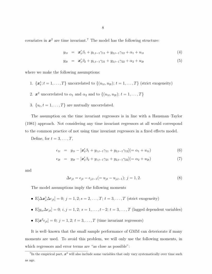
covariates in x2 are time invariant.7 The model has the following structure:
y1t = x′tβ1 + y1,t−1γ11 + y2,t−1γ12 + α1 + u1t (4)
y2t = x′tβ2 + y1,t−1γ21 + y2,t−1γ22 + α2 + u2t (5)
where we make the following assumptions:
1. {x1t ; t = 1, . . . , T} uncorrelated to {(u1t, u2t); t = 1, . . . , T} (strict exogeneity)
2. x2 uncorrelated to α1 and α2 and to {(u1t, u2t); t = 1, . . . , T}
3. {ut, t = 1, . . . , T} are mutually uncorrelated.
The assumption on the time invariant regressors is in line with a Hausman–Taylor
(1981) approach. Not considering any time invariant regressors at all would correspond
to the common practice of not using time invariant regressors in a fixed effects model.
Define, for t = 3, . . . , T ,
ε1t = y1t − [x′tβ1 + y1,t−1γ11 + y2,t−1γ12](= α1 + u1t) (6)
ε2t = y2t − [x′tβ2 + y1,t−1γ21 + y2,t−1γ22](= α2 + u2t) (7)
and
∆εjt = εjt − εj,t−1(= ujt − uj,t−1); j = 1, 2. (8)
The model assumptions imply the following moments
• E[∆x1s∆εjt] = 0; j = 1, 2; s = 2, . . . , T ; t = 3, . . . , T (strict exogeneity)
• E[yis∆εjt] = 0; i, j = 1, 2; s = 1, . . . , t−2; t = 3, . . . , T (lagged dependent variables)
• E[x2εjt] = 0; j = 1, 2; t = 3, . . . , T (time invariant regressors)
It is well–known that the small sample performance of GMM can deteriorate if many
moments are used. To avoid this problem, we will only use the following moments, in
which regressors and error terms are “as close as possible”:
7In the empirical part, x2 will also include some variables that only vary systematically over time such
as age.

9
• E[∆x1t ∆εjt] = 0; j = 1, 2; , t = 3, . . . , T ((strict) exogeneity)
• E[yi,t−2∆εjt] = 0; j = 1, 2; , t = 3, . . . , T (lagged dependent variables)
• E[x2εjt] = 0; j = 1, 2; t = 3, . . . , T (time invariant regressors)
For a given specification, i.e., given choices of x1t and x2, these moments can be used
for standard GMM estimation, separately for the equations for stocks and mutual funds.8
Any type of heteroskedasticity is allowed for, including that implied by the binary nature
of the dependent variable. Sargan tests for overidentifying restrictions are used to test the
validity of the moment restrictions. The assumption that the errors ujt are uncorrelated
error terms seems quite strong, but is common in this type of model. This assumption will
be tested by checking for second order autocorrelation in the residuals in the differenced
equations.9
3 Data
We use six waves of the CentER Savings Survey (CSS), drawn from 1993 until 1998.
Nyhus (1996) describes the set up of this data set and its general quality. The panel
consists of two samples. The first is designed to be representative of the Dutch population
(REP), but, due to survey non-response, the actual REP samples are not completely
representative. The REP contains approximately 2000 households in each wave, including
refreshment samples compensating for panel attrition. The second sample was drawn
from high-income areas and should represent the upper income decile (HIP). Initially, it
consisted of about 900 families. It is available in each wave except the final one. For
our analysis, we combine REP and HIP samples. In the descriptive statistics, we correct
for non-random sampling by using sample weights that are based upon income and home
ownership. These weights are constructed using information from a much larger data
8According to Blundell et al. (2000), additional moment restrictions based upon a mean stationarity
assumption can be used to improve efficiency. Specifications imposing these additional restrictions were
strongly rejected, however, and are therefore not discussed.9To estimate the linear probability model, we use the DPD98 software as described in Arellano and
Bond (1998).

10
set (Housing Needs Survey (WBO)) collected by Statistics Netherlands, which is close
to representative for the Dutch population. For observations with missing income, we
predict income from background variables such as family size and education level and age
of the head of the household.
The CSS data were collected via on-line terminal sessions, where each family was
provided with a PC and modem. The answers to the survey questions provide general
information on the household and its members, including work histories and labor market
status, health status, and many types of income. Important for our purposes are the ques-
tions on assets and debts. For most of the forty asset and debt categories, respondents
first indicate whether they own the type. If they do, they get a series of questions on
amounts and the precise nature of each asset in that category. Non–response in the own-
ership questions is negligible, but non–response in some of the questions on the amounts is
substantial. On average, about 20% of those who own stocks do not know or refuse to give
the value of their stocks. Mutual funds have a lower non–response rate of around 13% per
year. For some descriptive statistics (such as shares of specific asset types in total financial
assets, see below), the item non-response creates a problem. We have therefore imputed
the amounts for those who reported to be owners but did not provide an amount. See
Alessie et al. (2001), who also provide an extensive description of all categories of assets
and debts in the survey.
In the current paper, we focus on two types of risky financial assets: stocks and mutual
funds. The CSS distinguishes between two types of stocks: stocks from substantial holding
and (other) shares of private companies. There are very few people who hold the former
type, but these people typically hold high amounts. The two types of stocks are different
for tax purposes, since income from a substantial holding is treated as business capital.
Dividends from other shares and from mutual funds are liable to income tax to the extent
that they exceed an exemption threshold (Dfl 2,000 for couples, Dfl 1,000 for singles).
Capital gains on these are not taxed. The thresholds on dividends are separated from the
thresholds on interest on savings, creating a tax incentive for holding stocks or mutual
funds as well as saving accounts.
The first two columns of Table 1 show how ownership rates of the two types of assets

11
have developed during the years of the survey. The ownership rate of stocks has risen
from about 11% to more than 15%. Mutual funds were more often held than stocks,
with an even higher growth rate during the sample period. Many financial institutions
have been successful in presenting mutual funds as a low threshold asset, available to
many individual investors. Still, the majority of Dutch households held neither stocks nor
mutual funds in 1998. This lack of participation can be explained by monetary transaction
costs and information costs, both of which can be substantial.10
The remaining columns of Table 1 show the time path of amounts invested in stocks
and mutual funds, as shares of total financial assets.11 While the ownership rate of stocks
is always lower than the ownership rate of mutual funds, the reverse is true for the shares of
stocks and mutual funds in total financial wealth. This is because the few people who hold
stocks typically hold high amounts of them. The growth of the shares is less spectacular
than the growth of the ownership rates. The shares may be strongly influenced by some
large amounts, due to the skewed distribution of wealth and its components. Some rich
people hold large amounts, and there are very few of these in the sample, particularly
in 1998, the year without high income panel. This may explain why some of the time
patterns are not as pronounced as in aggregate data produced by Statistics Netherlands
(see Alessie et al. (2001)). In the remainder of the current paper, we will not use the
amounts data and focus on ownership rates.
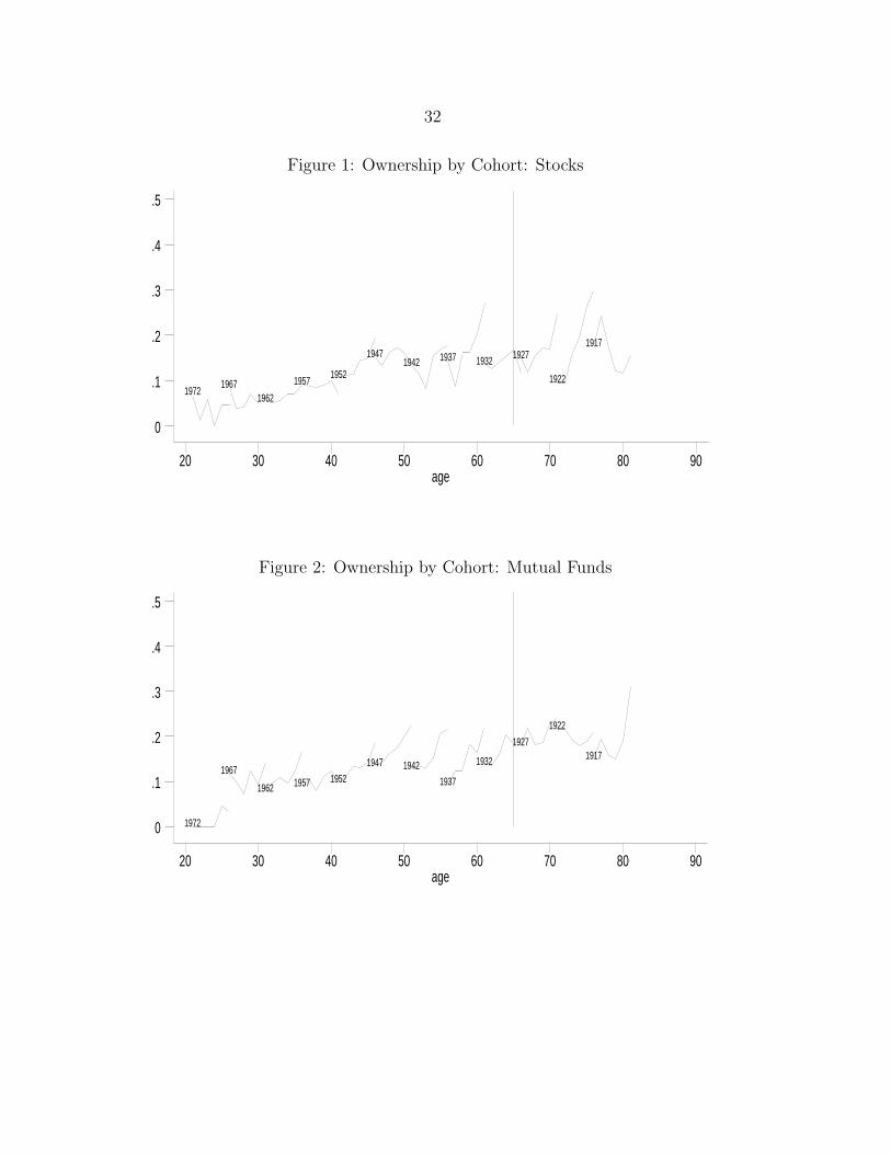
In Figures 1 and 2, we present (head of household) age and cohort patterns of the
ownership rates of stocks and mutual funds, based upon the six waves of the survey. We
use five year–of–birth cohorts, with birth years 1915–1919 for the oldest cohort, until birth
years 1970–1974 for the youngest cohort. Cohort labels indicate the middle year-of-birth.
10In the Netherlands, explicit transaction costs are low (about 0.5% of the investment) but implicit costs
(entry and exit fees incorporated in the buying and selling price of the fund) are higher. The maximum
entry fee is about 2.5% of the investment, and the maximum exit fee is about 1.5% (see Consumentenbond
(1999)). Apart from the transaction costs, most mutual funds charge a management fee of about 0.5% per
year and apply minimum investment restrictions. These implicit costs are comparable to the substantial
transaction costs in Italy discussed by Guiso and Jappelli (2001). It is not clear, however, whether Dutch
investors are aware of the implicit costs.11This is defined as the total amount invested in each asset by all households (weighted with the sample
weights), divided by (weighted) total financial wealth of all households.
12
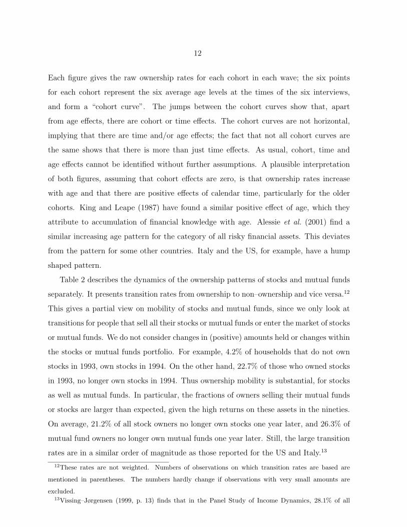
Each figure gives the raw ownership rates for each cohort in each wave; the six points
for each cohort represent the six average age levels at the times of the six interviews,
and form a “cohort curve”. The jumps between the cohort curves show that, apart
from age effects, there are cohort or time effects. The cohort curves are not horizontal,
implying that there are time and/or age effects; the fact that not all cohort curves are
the same shows that there is more than just time effects. As usual, cohort, time and
age effects cannot be identified without further assumptions. A plausible interpretation
of both figures, assuming that cohort effects are zero, is that ownership rates increase
with age and that there are positive effects of calendar time, particularly for the older
cohorts. King and Leape (1987) have found a similar positive effect of age, which they
attribute to accumulation of financial knowledge with age. Alessie et al. (2001) find a
similar increasing age pattern for the category of all risky financial assets. This deviates
from the pattern for some other countries. Italy and the US, for example, have a hump
shaped pattern.
Table 2 describes the dynamics of the ownership patterns of stocks and mutual funds
separately. It presents transition rates from ownership to non–ownership and vice versa.12
This gives a partial view on mobility of stocks and mutual funds, since we only look at
transitions for people that sell all their stocks or mutual funds or enter the market of stocks
or mutual funds. We do not consider changes in (positive) amounts held or changes within
the stocks or mutual funds portfolio. For example, 4.2% of households that do not own
stocks in 1993, own stocks in 1994. On the other hand, 22.7% of those who owned stocks
in 1993, no longer own stocks in 1994. Thus ownership mobility is substantial, for stocks
as well as mutual funds. In particular, the fractions of owners selling their mutual funds
or stocks are larger than expected, given the high returns on these assets in the nineties.
On average, 21.2% of all stock owners no longer own stocks one year later, and 26.3% of
mutual fund owners no longer own mutual funds one year later. Still, the large transition
rates are in a similar order of magnitude as those reported for the US and Italy.13
12These rates are not weighted. Numbers of observations on which transition rates are based are
mentioned in parentheses. The numbers hardly change if observations with very small amounts are
excluded.13Vissing–Jørgensen (1999, p. 13) finds that in the Panel Study of Income Dynamics, 28.1% of all

13
In Table 3, we present some evidence of correlation between holding one asset type
in one period, and holding the other asset type in the next period. For all years, the
ownership rate of stocks in year t + 1 is larger for those with mutual funds in year t than
for those without mutual funds in year t – conditional on not owning stocks in year t. For
example, 9.4% of those without stocks and with mutual funds in 1993 owned stocks in
1994. On the other hand, only 3.5% of those who had neither stocks nor mutual funds in
1993, owned stocks in 1994. Thus there is some positive correlation across ownership of the
two asset types. The same conclusion is obtained when ownership rates of mutual funds
are considered. Whether this positive correlation reflects some genuine state dependence
effect (such as learning) or (observed or unobserved) heterogeneity, is one of the issues we
will analyze in the next section, using the models in Section 2.
4 Results
The results of the random effects probit model and the linear probability model are
discussed in the first and second subsection, respectively. In the final subsection, the
implications of these results for explaining the growth in ownership rates of stocks and
mutual funds is presented. This is based on predicted probabilities, which are not always
between 0 and 1 in the linear probability models, and will therefore be done on the basis
of the probit results only.
4.1 Random Effects Probit
Tables 4a and 4b give the results for the bivariate probit model. The same explanatory
variables are used in both equations. Financial wealth is not included, since it may not be
strictly exogenous. In Appendix A, results are presented where lagged log financial wealth
households hold stocks in 1989 but not in 1994 or vice versa. Kennickell and Starr-McCluer (1997, p. 455)
consider ownership of one category consisting of stocks, mutual funds, managed investment accounts or
trusts in the Survey of Consumer Finances 1983–1989, and report transition rates of 10% from ownership
to non–ownership and 19% from non–ownership to ownership. Miniaci and Ruberti (2001) report two-
years transition rates from ownership to non-ownership between 32% and 42% using the SHIW survey of
the Bank of Italy.

14
and its own household specific average (over the observation window) are included. This
specification was chosen to control for the potential correlation between lagged financial
wealth and the individual effects (see Hausman and Taylor (1981), for example).14 We
do not discuss the results in Appendix A since most of them are qualitatively similar to
those in Tables 4a and 4b.
To avoid correlation with random effects and endogeneity of income and the marginal
tax rate, income is non-capital income and the marginal tax rate is the maximum of
the within–household imputed marginal rate applied to pseudo–taxable income, in which
individual capital income is replaced with its cross–sectional average (following Agell and
Edin (1990)). The effects of income and the marginal tax rate are hard to disentangle,
due to the strong (positive) correlation between these variables. We find that both effects
are positive for both types of assets. For stocks, the income effect is significant (at the
two-sided 5% level), while for mutual funds, the tax effect is significant. An explanation
for the stronger income effect for stocks than for mutual funds may be that high income
households will typically have more to invest, making the relatively large fixed costs
component of acquiring or holding individual stocks less important.
The income tax rules for stocks and mutual funds are the same (see Section 3). The
fact that capital gains are not taxed creates an incentive to hold stocks or mutual funds,
which increases with the household’s marginal tax rate.15 This explains the positive effect
of the marginal tax rate. The larger tax effect for mutual funds could be due to the fact
that suppliers of these funds strongly advertise their tax favored nature.
Labor market status variables for the head of household are jointly significant in both
equations. The most striking result is the enormous effect of self–employment on own-
ership of stocks: a self–employed head has a more than 25%-points higher probability
to own stocks than an employee (the reference group), ceteris paribus. Part of the ex-
planation could be that the self–employed often hold shares in their own firm which will
often be shares from a substantial holding. Excluding stocks from a substantial holding
from the analysis, however, hardly changes the size of the effect. Thus our result seems
14Including an arbitrary linear combination as in Hyslop (1999) is not possible due to the unbalanced
nature of the panel.15See Poterba (2001) for a general discussion of the impact of tax rules on portfolio choice.

15
rather different from what Heaton and Lucas (2000) find for the US: self–employed hold
more stocks in their own business, but hold less common stock, which is consistent with
precautionary behavior insofar as they assume less risk from other firms. The retired are
significantly more likely to own stocks or mutual funds than employees.
Since Figures 1 and 2 in the previous section have a plausible interpretation without
cohort effects, we have included age and time effects but no cohort effects. This identifies
the age and time patterns. Age is significantly positive for stocks as well as mutual funds.
This is in line with findings for risky assets ownership by King and Leape (1987), who at-
tribute the age effect to the accumulation of information about investment opportunities.
This information argument seems particularly relevant for individual stocks, since these
are the more “information intensive” type of risky assets. The time effects are similar for
the two asset types and show that the assets have become more popular during the last
few years of the survey (1997 and 1998; 1994 is the reference year).
The education variables are jointly significant in the equation for stocks only, indicating
that stocks are more often held by the higher educated. Again, this could be interpreted
as an effect of financial knowledge or interest in personal finance matters. If financial
wealth is included, however, the effects of education vanish (see Appendix A), implying
that the education effects in Table 3 might pick up wealth effects. A similar interpretation
can be given for the dummy “High Income Panel.” The positive significant effect of this
dummy for both asset types largely vanishes if financial wealth is included (Appendix A).
The way the high income sample is drawn makes it plausible that selection into this panel
is not only based upon income but also on wealth, explaining why the dummy variable
serves as a wealth proxy.
The estimated standard deviations of the random effects are 1.44 and 1.20 for stocks
and mutual funds, respectively. The standard deviations of the error terms are normalized
to one. Thus unobserved heterogeneity plays a major role, explaining more than half of
the unsystematic variation in the model.
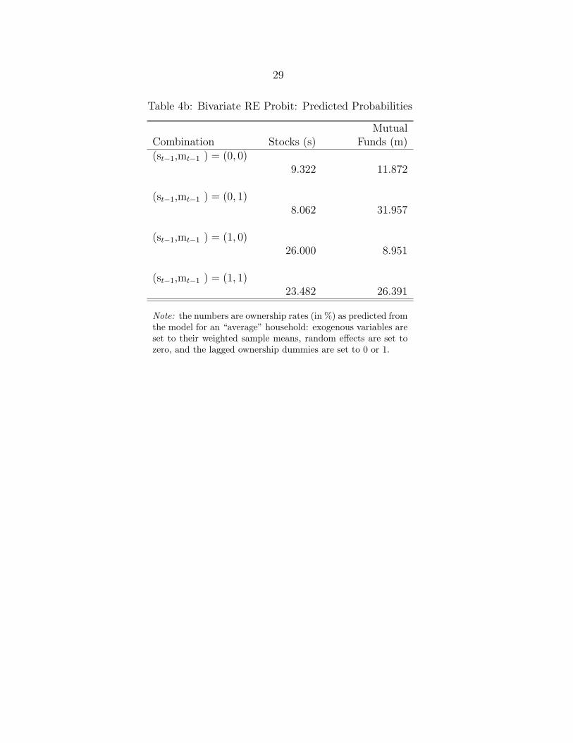
In both equations, the lagged dependent variables concerning ownership of the same
asset type are significantly positive. To interpret these results, predicted ownership prob-
abilities for the various lagged ownership states are presented in Table 4b. Exogenous

16
variables are set to their (weighted) sample means and random effects are set to zero.
Owners of stocks are about 16.7%-points more likely to own stocks next period than
non–owners with the same (observed and unobserved) characteristics if they do not own
mutual funds, and 15.4% points if they do hold mutual funds. For mutual funds, the
differences are even larger (20.1%-points if no stocks are held, 17.4% points if stocks are
held). Explanations for positive state dependence are the costs of acquiring stocks or
mutual funds (i.e., genuine transaction costs, not the costs of holding the assets)16 and
the information argument: once they own the asset, people are more familiar with it, and
are more aware of its risk and return characteristics.
All the results discussed so far relate to the dynamics of each of the two types of
assets separately. In most respects, these results are similar to what would be predicted
by separate univariate models. The bivariate model, however, also gives insight in the
relation between the two ownership decisions.
The “cross–effects” of lagged ownership of one asset type on ownership of the other
asset type are both negative and one of them is significant at the 5% level: ceteris paribus,
those who do not own stocks are significantly more likely to own mutual funds in the next
period than those who own stocks. According to Table 4b, the differences are 4.4%-points
and 2.9%-points for those who did and did not own mutual funds in the previous period.
If financial wealth is controlled for, the other cross–effect becomes significantly negative
also (see Tables A1a and A1b in Appendix A).
The negative cross–effects cannot be explained by a generic learning effect: if ownership
of one asset type would improve knowledge about the other asset type, a positive cross–
effect would result. On the other hand, these are consistent with the same adjustment
cost arguments that explained the strong positive effects of lagged ownership of the same
asset type. People who own stocks but no mutual funds have an incentive to remain
focused on stocks to avoid the adjustment costs, while people who own neither stocks nor
mutual funds and who consider investing in risky assets, face adjustment costs anyhow.
Adjustment costs thus give an explanation for own as well as cross state dependence
16Hyslop (1999) formalizes this in a stylized dynamic optimization model; a similar model can be used
here for each of the two assets separately.

17
effects, while learning can only explain the univariate effects. These adjustment costs
may reflect the actual (monetary) transaction costs involved with buying or selling an
asset, but may also include non-monetary components such as the required effort, the
need to collect information, etc.
The estimated correlation coefficient between the two random effects is large: 0.659
(with standard error 0.055). This suggests that the people who have a large preference
for holding stocks (given their observed characteristics), tend to be the same people who
have a preference for holding mutual funds. These may be the people with lower degrees
of risk aversion or higher interest in financial markets. The positive correlation between
holding stocks and holding mutual funds in the data, is to a large extent due to this
positive correlation in unobserved heterogeneity.17
Allowing for correlation in the individual effects in the two equations has a major
impact on the estimates of the cross–effects of ownership of one type of asset on owner-
ship of the other type of asset in the next time period. If we estimate the model with
the correlation between the random effects restricted to zero, we find significant positive
estimates for both cross–effects. Not allowing for correlation between unobserved hetero-
geneity terms would thus lead to a large upwards bias on the effect of ownership of one
asset type on ownership of the other type.
The correlation between the error terms in the two equations is small and insignificant.
A negative correlation could point at fixed holding costs for each asset type (such as
monitoring costs) that would be an incentive for specialization. Vissing–Jørgensen (1999)
finds evidence of such costs. A positive correlation could point at a common element in
monitoring both assets, or at benefits of diversification. Apparently, the positive and the
negative effects cancel or do not play a role.
4.2 Linear Probability Model
Several specifications of the linear probability model of Section 2.2 are estimated, with
different choices for xt = (x1t ,x
2t ). On the basis of Sargan tests for the over–identifying
17The correlation drops somewhat if financial wealth is included, but remains significant (see Table
A1b).
18
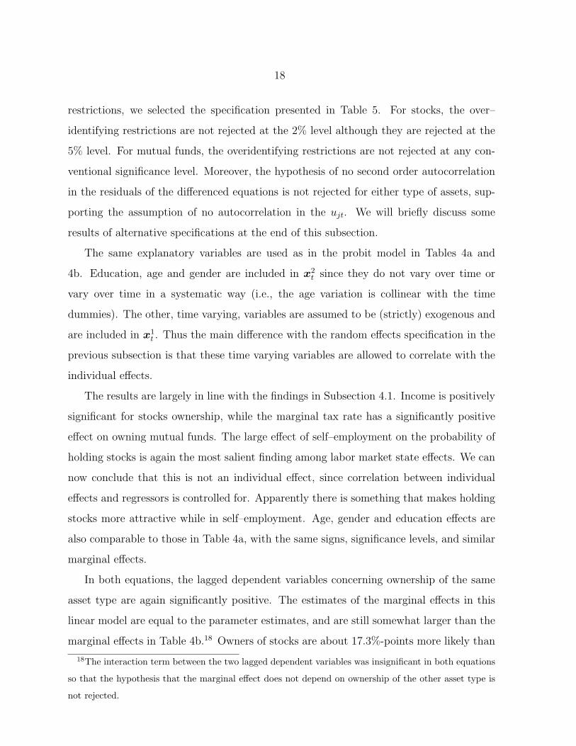
restrictions, we selected the specification presented in Table 5. For stocks, the over–
identifying restrictions are not rejected at the 2% level although they are rejected at the
5% level. For mutual funds, the overidentifying restrictions are not rejected at any con-
ventional significance level. Moreover, the hypothesis of no second order autocorrelation
in the residuals of the differenced equations is not rejected for either type of assets, sup-
porting the assumption of no autocorrelation in the ujt. We will briefly discuss some
results of alternative specifications at the end of this subsection.
The same explanatory variables are used as in the probit model in Tables 4a and
4b. Education, age and gender are included in x2t since they do not vary over time or
vary over time in a systematic way (i.e., the age variation is collinear with the time
dummies). The other, time varying, variables are assumed to be (strictly) exogenous and
are included in x1t . Thus the main difference with the random effects specification in the
previous subsection is that these time varying variables are allowed to correlate with the
individual effects.
The results are largely in line with the findings in Subsection 4.1. Income is positively
significant for stocks ownership, while the marginal tax rate has a significantly positive
effect on owning mutual funds. The large effect of self–employment on the probability of
holding stocks is again the most salient finding among labor market state effects. We can
now conclude that this is not an individual effect, since correlation between individual
effects and regressors is controlled for. Apparently there is something that makes holding
stocks more attractive while in self–employment. Age, gender and education effects are
also comparable to those in Table 4a, with the same signs, significance levels, and similar
marginal effects.
In both equations, the lagged dependent variables concerning ownership of the same
asset type are again significantly positive. The estimates of the marginal effects in this
linear model are equal to the parameter estimates, and are still somewhat larger than the
marginal effects in Table 4b.18 Owners of stocks are about 17.3%-points more likely than
18The interaction term between the two lagged dependent variables was insignificant in both equations
so that the hypothesis that the marginal effect does not depend on ownership of the other asset type is
not rejected.

19
otherwise identical non-owners of stocks to own stocks next period. Owners of mutual
funds are about 20.4%-points more likely than non-owners of mutual funds to own mutual
funds in the next period.
The main difference with Table 4b is the estimated “cross–effect” of lagged ownership
of stocks on ownership of mutual funds. In Table 5, the effect is positive and insignificant,
whereas it was negative and significant in the random effects probit model. This confirms
that no evidence of learning is found, but does not support the adjustment costs argument
given in the previous subsection.
Detailed results for alternative specifications are available upon request. One alterna-
tive is to exclude age, education and gender variables completely. This would correspond
to the pure fixed effects model. Results for this model are similar to those in Table 5. For
stocks as well as mutual funds, Sargan tests do not reject the over-identifying restrictions
(significance probabilities 0.110 and 0.087) and tests for second order autocorrelation do
not reject the assumption of error terms that are uncorrelated over time (significance
probabilities 0.872 and 0.226). This specification gives similar effects of the time varying
regressors as Table 5, and similar effects of lagged ownership of the asset type itself (0.181
for stocks and 0.191 for mutual funds, both significant). The main difference is that the
effect of lagged ownership of mutual funds on ownership of stocks is now significantly
negative (−0.084, with standard error 0.039), while that of lagged stocks on ownership of
mutual funds remains insignificant and positive (0.009 with standard error 0.051).
Models which make more restrictive assumptions on the relation between error terms
and time varying explanatory variables (such as zero correlation with individual effects or
mean stationarity) are clearly rejected by the Sargan tests for over-identifying restrictions,
although they give similar qualitative conclusions on the ownership dynamics. A model
that includes lagged log financial wealth as a weakly exogenous variable in x1t also gives
similar results to those in Table 5, particularly concerning the dynamics. These results
imply a significantly negative effect of financial wealth on future ownership of stocks and
mutual funds, as in the probit model in Table A1a in Appendix A.
The main purpose of the linear probability models is to perform a sensitivity check
on the findings on the basis of the probit models. The conclusion is that most findings

20
are very similar: the tax and income effects, the effect of labor market position, in casu
self–employment, and the effects of lagged ownership of stocks on ownership of stocks and
of lagged ownership of mutual funds on ownership of mutual funds. The only differences
concern the cross–effects of lagged ownership of stocks on ownership of mutual funds
and of lagged ownership of mutual funds on ownership of stocks. Still, we always find a
significant negative effect or an insignificant effect, and we do not find significant positive
effects unless we impose a zero correlation of unobserved heterogeneity terms for the two
equations — a restriction that is always fiercely rejected. This confirms that cross–effects
due to learning cannot be established, while there is some evidence of cross–effects due
to adjustment costs.
4.3 Explaining the Growth in Ownership Rates
The probit model results presented in Table 4a can be used to predict ownership proba-
bilities for individual households and aggregate ownership rates for groups of households
under different scenarios. Such predictions can be used to analyze how much the explana-
tory variables in the equations contribute to the changes in the aggregate ownership rates
of stocks and mutual funds over time. The idea is similar to the Oaxaca decomposition
that is commonly used in studies on wage differentials (Oaxaca, 1973).
The results are presented in Table 6. The top panel refers to stocks, the bottom
panel to mutual funds. The first row of each panel presents observed changes in mean
predicted ownership rates (in percentage points), using common samples for the two years
considered. Random effects are set to zero. Since time dummies for all years are included,
these sample changes reflect the increasing trend in aggregate ownership rates over the
same years reasonably well.19 The other rows compare two sets of predicted aggregate
ownership rates: those using the observed explanatory variables and those in which one
or more explanatory variables are replaced by their lags. Take, for example, the change in
the stocks ownership rate from 1997 to 1998 of about 3.48%-points. If in the 1998 sample
age is replaced by its lagged value (i.e., age in 1997), the predicted mean ownership rate
19This should still improve if random effects were integrated out instead of set to zero, but then the
correlation between random effects and lagged ownership dummies should be accounted for.

21
falls by 0.26%-points. Thus the age effect explains 0.26%-points of the total rise of 3.48%
points. Similarly, changes in marginal tax rates (which become somewhat larger, on
average) explain a 0.16%-points rise of the ownership rate. All exogenous regressors (not
including time dummies or lagged dependent variables) explain a rise of about 0.44%-
points. The lagged dependent variables explain a rise of 0.11% points. This is mainly
due to the rise in the ownership rate of stocks from 1996 to 1997. In total the regressors
in the model (time dummies not included) thus explain 0.55%-points of the 3.48%-points
rise in ownership of stocks. The remainder is not explained by the regressors and mainly
captured by the time dummies. The contribution of the time dummies can be seen as the
(residual) part of the change in ownership that cannot explained by the economic variables
in the model.20 We find that the economic variables age referring to labor market status,
and lagged ownership explain part of the rise in ownership, but most of it is a time trend
not captured by the explanatory variables in the model. The results for mutual funds
are similar. The conclusion is that age is the only exogenous variable which consistently
positively contributes to explaining the rising ownership rates. The main reason is that
age is not only significant in the probits but also systematically increases over time. Self-
employment, for example, is very important for ownership of stocks, but the fraction of
self–employed in the sample does not vary systematically over the years.
5 Conclusions
As the stockholder base has widened considerably over the last decade in many countries,
understanding how households make their portfolio decisions over time has wide–ranging
implications for understanding the allocation of risk in financial markets, the distribution
of wealth, and pricing relationships for individual assets. This paper is one of the first
studies of the dynamics of individual households’ (multivariate) investment strategies
using representative panel survey data.
We have estimated dynamic models explaining ownership of the two main types of
20This can be compared to the changes “explained by” parameter changes in the usual Oaxaca decom-
position; in this model with time dummies, only the constant term can vary over time.

22
risky financial assets in the Netherlands: stocks and mutual funds. The main difference
between the two is that mutual funds are an easy way to attain diversification, at the cost
of a premium paid to the mutual funds provider. This makes mutual funds particularly
attractive for small investors with little financial knowledge. Our results confirm this to
some extent, since we find that the probability to own stocks increases significantly with
income while the probability to own mutual funds does not. Tax incentives, on the other
hand, play a larger role for mutual funds than for stocks. Self–employed are much more
likely to hold stocks than others, while they do not have a different ownership rate of
mutual funds. An explanation could be that the self–employed are interested in specific
stocks to hedge against their larger income uncertainty. The alternative explanation that
the self–employed simply have different preferences and care less about diversification,
is unlikely since the effect remains the same if unobserved (preference) heterogeneity is
allowed to be correlated with background variables in a fixed effects setting.
We find that the dynamics of ownership of either type of risky assets are driven by
state dependence as well as unobserved heterogeneity. Both explain part of the persistence
of ownership of both types of assets in the data. The state dependence can be explained
from the adjustment costs of buying or selling the asset. On the other hand, the positive
sample correlation between ownership of one type of asset and lagged ownership of the
other asset is explained from (observed and unobserved) heterogeneity only. One source of
this could be a joint element in monitoring or other holding costs that makes it attractive
to hold both asset types simultaneously. Another reason could be that combining stocks
and mutual funds creates opportunities for diversification that cannot be attained by
mutual funds alone (since these typically invest in certain sub-samples of stocks).
We find no evidence that households substitute one type of assets by the other, or
that ownership of one type leads to more financial knowledge and a larger probability of
buying the other type of assets. In contrast, we find some evidence of a negative effect
of owning one type of assets on buying or keeping the other type. This can be explained
by adjustment costs, which imply that those who have acquired one specific asset will
tend not to reallocate their money to the other type of assets. Such adjustment costs will
comprise the actual transaction costs involved with portfolio adjustment, but may also

23
contain non–monetary or perceived costs components, reflecting the required effort, the
costs of acquiring information, etc.
Classical papers like those of Merton (1969) and Samuelson (1969) assume that agents
live in a frictionless world and have HARA preferences. They predict myopic optimal
behavior (i.e. a constant fraction of risky assets in the portfolio) for a given individual.
To make such models more realistic, it would be useful to introduce dynamic features.
Our results suggest that adjustment costs are particularly relevant.
Future research can go in several directions. First, we have not modelled the amounts
held. Although this is not without measurement problems, it certainly seems a relevant
extension. It could also help analyze the importance of fixed costs of holding, buying,
and selling assets, extending the work of Vissing–Jørgensen (1999). Second, if data for a
longer time period become available, it seems useful to relate the ownership dynamics to
the trends in the financial markets or to relevant macro variables such as unemployment,
inflation or expected inflation, consumer confidence, etc. Third, straightforward exten-
sions of our models could be used to analyze other asset and debt types, or to analyze
assets at a less aggregate level. For example, to understand the dynamics and in partic-
ular the underlying cost structure driving these, it seems relevant to distinguish people
who substitute one stock for the other from people who do not trade at all.
Finally, it would be interesting to extend the analysis with data on the recent time
period with falling asset returns. The rationale for people then not venturing into risky
assets seems to be that the return foregone is too low compared to the costs saved. In
times when returns are high (1993-1998), this may make sense, and the time dummies in
our models seem to pick up the sluggishness in the adjustment. On the other hand, there
is some asymmetry in the sense that once adjustment costs are incurred, part of them
will be sunk (at least the information acquisition costs). Selling the assets will therefore
not be associated with the same costs. It therefore seems interesting to see what happens
if times are bad.
24
References
Agell, J. and P.–A. Edin (1990), “Marginal Taxes and the Asset Portfolios of SwedishHouseholds,” Scandinavian Journal of Economics, 92, 47–64.
Alessie, R., S. Hochguertel and A. van Soest (2001), “Household Portfolios in the Nether-lands”, Chapter 9 in Guiso et al. (2001).
Arellano, M. and S.R. Bond (1998), “Dynamic Panel Data Using DPD98 for GAUSS,”Institute for Fiscal Studies, mimeo.
Blundell, R., S. Bond and F. Windmeijer (2000), “Estimation in Dynamic Panel DataModels: Improving on the Performance of the Standard GMM Estimators,” in B. Balt-agi (ed.), Nonstationary Panels, Panel Cointegration, and Dynamic Panels. Advancesin Econometrics, 15, JAI Press, Amsterdam.
Chay, K. and D. Hyslop (2000), “Identification and Estimation of Dynamic Binary Re-sponse Panel Data Models: Empirical Evidence using Alternative Approaches,” mimeo,University of California at Berkeley.
Consumentenbond (1999), Jaarboek Beleggen 1999, Kosmos, Utrecht.
Guiso, L., and T. Jappelli (2001), “Household Portfolios in Italy”, Chapter 7 in Guisoet al. (2001).
Guiso, L., M. Haliassos and T. Jappelli, eds. (2001), Household Portfolios, MIT PressCambridge Mass., in press.
Hajivassiliou, V.A. and P.A. Ruud (1994), “Classical Estimation Methods for LDV ModelsUsing Simulation,” in: R.F. Engle and D.L. McFadden (eds.), Handbook of Economet-rics, vol. IV, North–Holland, New York, 2384–2443.
Hausman, J.A. and W.E. Taylor (1981), “Panel Data and Unobservable Individual Ef-fects,” Econometrica, 49, 1377–1398.
Heaton, J., and D. Lucas (2000), “Portfolio Choice and Asset Prices: The Importance ofEntrepreneurial Risk,” Journal of Finance, 55, 1163–1198.
Heckman, J. (1981a), “Statistical Models for Discrete Panel Data,” in C.F. Manski andD.L. McFadden (eds.), Structural Analysis of Discrete Data with Econometric Appli-cations, MIT Press, London, 114–178.
Heckman, J. (1981b), “The Incidental Parameters Problem and the Problem of InitialConditions in Estimating a Discrete Time-Discrete Data Stochastic Process,” in C.F.Manski and D.L. McFadden (eds.), Structural Analysis of Discrete Data with Econo-

25
metric Applications, MIT Press, London, 179–195.
Hyslop, D.R. (1999), “State Dependence, Serial Correlation and Heterogeneity in In-tertemporal Labor Force Participation of Married Women,” Econometrica, 67, 1255–1294.
Kennickell, A.B. and M. Starr-McCluer (1997), “Retrospective reporting of householdwealth: Evidence from the 1983-1989 Survey of Consumer Finances,” Journal of Busi-ness & Economic Statistics, 15, 452-463.
King, M. A. and J. I. Leape (1987), “Asset Accumulation, Information, and the LifeCycle,” NBER Working Paper, No. 2392.
Lee, L.–F. (1997), “Simulated Maximum Likelihood Estimation of Dynamic DiscreteChoice Statistical Models Using some Monte Carlo Results,” Journal of Economet-rics, 82, 1-35.
Merton, R.C. (1969), “Lifetime Portfolio Selection under Uncertainty: The ContinuousTime Model,” Review of Economics and Statistics, 51, 247–257.
Miniaci, R. and F. Ruberti (2001), “Household Risky Asset Ownership: A DynamicAnalysis,” Universita di Padova, mimeo.
Nyhus, E.K. (1996), “The VSB-CentER Savings Project: Data Collection Methods, Ques-tionnaires and Sampling Procedures,” VSB-CentER Savings Project Progress Reportno. 42, Tilburg University.
Oaxaca, R.L. (1973), “Male–Female Wage Differentials in Urban Labor Markets,” Inter-national Economic Review, 14, 693-709.
Poterba, J.M. (2001), “Taxation and Portfolio Structure: Issues and Implications,” Chap-ter 3 in Guiso et al. (2001).
Samuelson, P.A. (1969), “Lifetime Portfolio Selection by Dynamic Stochastic Program-ming,” Review of Economics and Statistics, 51, 239–246.
Verbeek, M. (2000), A Guide to Modern Econometrics, Wiley, Chichester.
Vissing–Jørgensen, A. (1999), “Towards an Explanation of Household Portfolio ChoiceHeterogeneity: Nonfinancial Income and Participation Cost Structures,” mimeo, De-partment of Economics, University of Chicago.

26
Tables and Figures
Table 1: Ownership Rates and Portfolio Shares
ownership rate portfolio sharemutual mutual
year stocks funds stocks funds1993 11.4 11.8 21.3 5.41994 9.9 12.8 20.6 6.71995 11.4 12.9 22.0 6.21996 13.5 14.7 24.0 7.01997 14.4 16.2 25.3 7.11998 15.4 18.4 23.8 10.0
Note: weighted statistics; portfolio share: ratio of wealth held in stocksor mutual funds to total financial assets
Table 2: Transition Rates (Univariate)
ownership → non–ownershipnon–ownership → ownership
years mutual mutualt/t + s stocks funds stocks funds
1993/94 22.7 26.5 4.2 6.8(309) (310) (1768) (1767)
1994/95 26.7 32.5 5.5 6.1(288) (335) (1592) (1545)
1995/96 21.2 20.1 6.1 5.7(274) (298) (1406) (1382)
1996/97 19.7 26.1 6.0 8.2(239) (253) (1172) (1158)
1997/98 15.7 26.3 4.4 7.6(159) (190) (838) (807)
1993/97 25.8 36.2 11.6 12.4(128) (138) (673) (663)
Note: unweighted statistics; transition rate ownership→ non–ownership, t/t+s= 100 (number of households who own in year t but not in year t+s)/(numberof owners in year t). Total cell sizes (corresponding to 100%) in parentheses.

27
Table 3: Transition Rates (Bivariate)
ownership proba-ownership year t bility in t + s
years mutual mutualt/t + s stocks funds stocks funds
1993/94 no no 3.5 5.4yes no 75.3 17.8no yes 9.4 73.9yes yes 81.3 72.9
1994/95 no no 4.5 5.8yes no 72.5 8.4no yes 12.0 65.8yes yes 74.6 70.9
1995/96 no no 4.4 5.0yes no 78.7 11.0no yes 17.6 77.7yes yes 79.1 83.6
1996/97 no no 5.3 7.1yes no 78.7 16.9no yes 10.7 70.0yes yes 82.5 79.6
1997/98 no no 3.0 6.9yes no 87.7 13.6no yes 13.4 71.4yes yes 80.8 76.9
1993/97 no no 9.4 10.9yes no 74.4 22.1no yes 25.0 64.6yes yes 73.8 61.9
Note: See Table 2

28
Table 4a: Bivariate Random Effects Probit
Stocks Mutual FundsVariable Name Estimate Std.Err. Estimate Std.Err.constant –4.8132 0.4400 –3.4065 0.3213stockst−1 1.1909 0.1077 –0.2540 0.1232mutual fundst−1 –0.1401 0.1073 1.1144 0.0946age 0.0210 0.0054 0.0091 0.0044education
intermediate 0.3623 0.1797 0.0491 0.1547vocational 0.0372 0.1375 0.0225 0.1124high 0.4054 0.1628 0.2161 0.1307Wald (p–value) 0.0028 0.2039
log income 0.0522 0.0182 0.0219 0.0171HH marg. tax rate 0.6158 0.3408 1.2520 0.2623high–income panel 1.0030 0.1414 0.5981 0.1027labor market status
unemployed 0.1552 0.3431 –0.0121 0.2814retired 0.3142 0.1519 0.3857 0.1274disabled –0.5144 0.3592 0.1424 0.2316self–employed 1.5511 0.1695 0.1317 0.1538other 0.4810 0.2371 –0.0329 0.1889Wald (p–value) 0.0000 0.0487
female –0.4962 0.1536 –0.0736 0.1117year
1995 0.0614 0.0855 –0.0661 0.07391996 0.2101 0.0966 0.0483 0.09041997 0.3542 0.1090 0.2106 0.08721998 0.6144 0.1378 0.3089 0.1039Wald (p–value) 0.0001 0.0021
σα 1.4446 0.1602 1.2027 0.1241ρα 0.6590 0.0549ρ 0.0260 0.0653
Number of households 2861Number of observations 9680Log–likelihood –5706.42
Note: Estimates of the initial conditions equations are available upon request.
29
Table 4b: Bivariate RE Probit: Predicted Probabilities
MutualCombination Stocks (s) Funds (m)(st−1,mt−1 ) = (0, 0)
9.322 11.872
(st−1,mt−1 ) = (0, 1)8.062 31.957
(st−1,mt−1 ) = (1, 0)26.000 8.951
(st−1,mt−1 ) = (1, 1)23.482 26.391
Note: the numbers are ownership rates (in %) as predicted fromthe model for an “average” household: exogenous variables areset to their weighted sample means, random effects are set tozero, and the lagged ownership dummies are set to 0 or 1.

30
Table 5: Linear Probability Models
Stocks Mutual FundsVariable Name Estimate Std.Err. Estimate Std.Err.constant –0.1403 0.0540 –0.1368 0.0566stockst−1 0.1734 0.0541 0.0102 0.0503mutual fundst−1 –0.0640 0.0392 0.2044 0.0494age 0.0025 0.0009 0.0035 0.0009education
intermediate 0.0603 0.0270 0.0063 0.0249vocational 0.0148 0.0178 –0.0028 0.0171high 0.0747 0.0259 0.0442 0.0243
log income 0.0073 0.0034 0.0015 0.0032HH marg. tax rate –0.0436 0.0444 0.1284 0.0621high–income panel 0.1439 0.0211 0.0849 0.0212labor market status
unemployed 0.0070 0.0290 0.0230 0.0283retired 0.0476 0.0293 –0.0263 0.0321disabled 0.0257 0.0386 0.0048 0.0395self–employed 0.2239 0.0580 0.0105 0.0369other 0.0461 0.0232 –0.0197 0.0260
female –0.0395 0.0160 –0.0164 0.0170year
1996 0.0176 0.0074 0.0033 0.00771997 0.0347 0.0093 0.0365 0.01091998 0.0638 0.0124 0.0539 0.0147
Number of households 1870Number of observations 5950Sargan, 14df (p−value) 26.7231 0.021 19.1600 0.159AR(2) test (p−value) 0.094 0.925 1.336 0.181

31
Table 6: Oaxaca Decompositions of Changes in Ownership Rates (in %-points)
years 1993/94 1994/95 1995/96 1996/97 1997/98 1993/97Change inownership rate StocksTotal change n.a. 1.40 1.87 1.85 3.48 n.a.exlained by
change in . . .stockst−1 &mutual fds.t−1 n.a. 0.09 0.29 0.17 0.11 n.a.education 0.00 0.04 0.00 –0.00 0.01 0.02age 0.19 0.21 0.23 0.24 0.26 1.10log income 0.16 –0.02 –0.02 –0.22 0.16 –0.02tax rate 0.08 –0.03 –0.02 –0.12 0.06 –0.20tax & income 0.23 –0.07 –0.05 –0.36 0.20 –0.25labor market 0.00 0.50 –0.02 0.02 –0.02 0.69all x-s 0.42 0.70 0.18 –0.09 0.44 1.62time dummies 0.00 0.60 1.57 1.61 3.03 n.a.
Change inownership rate Mutual FundsTotal change n.a. –0.71 1.71 2.29 1.80 n.a.exlained by
change in . . .stockst−1 &mutual fds.t−1 n.a. 0.27 –0.25 0.12 0.16 n.a.education 0.00 0.04 –0.00 0.00 0.01 0.04age 0.12 0.12 0.13 0.14 0.14 0.60log income 0.07 0.00 0.00 –0.10 0.07 0.03tax rate 0.13 –0.08 –0.10 –0.34 0.15 –0.56tax & income 0.18 –0.09 –0.11 –0.47 0.20 –0.59labor market 0.00 0.18 0.12 0.14 0.06 0.65all x-s 0.29 0.25 0.13 –0.18 0.43 0.74time dummies 0.00 –0.88 1.55 2.35 1.49 n.a.
Note: Based on weighted means of (univariate normal) ownership probabilities as pre-dicted from equations (1) and (2), with random effects set to zero; presented are thedifferences in such means between the baseline case and the case where some regressorsare lagged: “total change”: all right hand side variables are lagged, including ownershipdummies and time dummies; “all x-s”: all regressors except time dummies and laggedownership dummies are lagged.
32
Figure 1: Ownership by Cohort: Stocks
Figure 1: Ownership by Cohort: Stocks
age20 30 40 50 60 70 80 90
0
.1
.2
.3
.4
.5
.6
.7
.8
.9
1
1917
1922
19271932193719421947
19521957
19621967
1972
Figure 2: Ownership by Cohort: Mutual Funds
Figure 2: Ownership by Cohort: Mutual Funds
age20 30 40 50 60 70 80 90
0
.1
.2
.3
.4
.5
.6
.7
.8
.9
1
1917
1922
1927
1932
1937
19421947
195219571962
1967
1972

33
A Alternative Specification
Table A1a: Bivariate Random Effects Probit (Alternative Specification)
Stocks Mutual FundsVariable Name Estimate Std.Err. Estimate Std.Err.constant –12.5107 1.6092 –9.4148 1.0226stockst−1 1.1531 0.1575 –0.4358 0.1831mutual fundst−1 –0.4175 0.1630 0.9944 0.1415age 0.0008 0.0074 –0.0124 0.0062education
intermediate –0.0216 0.2592 0.0152 0.1984vocational 0.0307 0.2001 –0.0268 0.1508high 0.2577 0.2305 0.0789 0.1738Wald (p–value) 0.4469 0.8696
log income 0.0824 0.0267 0.0123 0.0230HH marg. tax rate 0.1087 0.4680 0.9149 0.3561high–income panel 0.1288 0.1454 –0.0711 0.1195log. fin. wealtht−1 –0.1089 0.0504 –0.0925 0.0554log. fin. wealth (avg.) 0.9535 0.1235 0.8048 0.0992labor market status
unemployed 0.5903 0.4752 –0.1068 0.4148retired 0.4507 0.2079 0.4781 0.1789disabled –0.1927 0.5550 0.2038 0.3207self–employed 1.3236 0.2428 –0.4412 0.2180other 0.5131 0.3815 0.2807 0.3226Wald (p–value) 0.0000 0.0219
female –0.1328 0.1794 0.2111 0.1520year
1996 0.1406 0.1065 0.1288 0.10061997 0.2737 0.1294 0.3247 0.10121998 0.5503 0.1705 0.4428 0.1247Wald (p–value) 0.0123 0.0011
σα 1.4101 0.2223 1.1605 0.1787ρα 0.6074 0.0995ρ –0.1169 0.0910
Number of households 1871Number of observations 5953Log–likelihood –3401.50
Note: see Table 4a.

34
Table A1b: Bivariate RE Probit: Predicted Probabilities
MutualCombination Stocks (s) Funds (m)(st−1,mt−1 ) = (0, 0)
5.638 7.440
(st−1,mt−1 ) = (0, 1)3.382 21.339
(st−1,mt−1 ) = (1, 0)17.909 4.197
(st−1,mt−1 ) = (1, 1)12.295 14.026
Note: see Table 4b.

35
B Details on Model and Estimation Technique
This appendix presents some details of the econometric model described in Section 2.1.This is a bivariate random effects probit model with Gaussian errors. It is estimated bySimulated Maximum Likelihood.
Model
For a household (the index of the household will be suppressed) that is observed in wavest = 1, . . . , T , the latent variable model for time periods t = 2, . . . , T is given by
y?1t = x′tβ1 + y1,t−1γ11 + y2,t−1γ12 + α1 + u1t
y?2t = x′tβ2 + y1,t−1γ21 + y2,t−1γ22 + α2 + u2t (B1)
We observe yjt = 1[y?jt > 0], cf. (3). The β’s and γ’s are unknown parameters. The regres-
sor vector x includes a constant term. Note that it would be straightforward to extend thismodel by adding interaction terms involving the lagged dependent variables. For instance,y1,t−1γ12 can be replaced by y1,t−1x
′t ˜gamma12, where γ12, terms y1,t−1y2,t−1δj, j = 1, 2 can
be added to the first and second equation, etc. The model as it is presented here is themodel for which we present the results.
We assume that the errors ujt are independent over time, and that u1t, u2t follows anormal distribution, with unit variances and a cross–equation correlation Cov(u1t, u2t) =ρ. The random effects αj are assumed to be normally distributed with covariance matrix
Σα =
(σ2
α1σα1σα2ρα
· σ2α2
). (B2)
For the initial period t = 1, Model (B1) would imply
y?11 = x′1β1 + y1,0γ11 + y2,0γ12 + α1 + u11
y?21 = x′1β2 + y1,0γ21 + y2,0γ22 + α2 + u21 (B3)
Data at times t = 0,−1,−2, . . . are not available, however. For the univariate case,Heckman (1981b) suggests to replace the equation for t = 1 by a static equation withdifferent regression coefficients and arbitrary linear combinations of the random effects.This can be seen as an approximation to the “reduced form”. For the bivariate model,this yields
y?11 = x′1κ1 + λ11α1 + λ12α2 + ε11
y?21 = x′1κ2 + λ21α1 + λ22α2 + ε21 (B4)
In a univariate framework, Chay and Hyslop (2000) also discuss an alternative specifica-tion that imposes a relation between the parameters in these equations and the parametersin model (B1), but they find that the estimator based upon this specification performs notas good as the specification without these restrictions. We will therefore not impose suchrestrictions and allow the parameters in the initial equations to be completely differentfrom the parameters in the dynamic equations. The error terms ε11 and ε21 in (B4) arestandard normal with correlation coefficient ρε.

36
Estimation
The likelihood contribution for a given household can be written as the expected value ofthe log likelihood contribution conditional on the random effects. It is of the form
F =
∫ +∞
−∞
∫ +∞
−∞h(α1, α2) g2(α1, α2, Σα) dα1dα2 (B5)
where g2(·) is the bivariate normal density of the random effects (α1, α2). See (B8) belowfor the exact expression of the function h.
Standard approaches of numerically integrating out the random effects are feasible butdifficult.21 Instead, we approximate the expectation in (B5) with the simulated average
F =1
R
R∑r=1
h(αr1, α
r2). (B6)
where the random effects (α1, α2) are replaced by independent random draws (αr1, α
r2),
constructed as follows:If N is the number of households in the sample, 2RN independent draws from the
standard normal distribution are taken (using a pseudo–random number generator). Foreach household, this gives 2R independent draws αr
1, r = 1, . . . , R and αr2, r = 1, . . . , R
from the univariate standard normal distribution. These draws remain fixed during theestimation process.
To approximate the likelihood at given parameter values, the (αr1, α
r2) are transformed
into draws from a bivariate normal distribution with zero means and covariance matrixΣα, using a Cholesky decomposition of Σα. This step is performed inside the likelihoodroutine because the parameters in Σα are updated at every iteration. The link betweenαr
j and αrj is
αr1 = σα1α
r1
αr2 = σα2ρααr
1 + σα2
√1− ρ2
ααr2 (B7)
The resulting estimator will be asymptotically equivalent to Maximum Likelihood ifR/√
N → +∞ (see Hajivassiliou and Ruud (1994), for example). For maximizationof the log–likelihood function, we use the BHHH algorithm, based on first derivatives.
Likelihood contributions
A given household is observed in T waves. Hence the likelihood contribution (B5) is afunction of
h(α1, α2) = Φ2
(y11µ11, y21µ21, y11y21ρε
∣∣∣x1
)×
×T∏
t=2
Φ2
(y1tµ1t, y2tµ2t, y1ty2tρ
∣∣∣y1,t−1, y2,t−1, y1,t−2, y2,t−2, . . . , xt
) (B8)
21The most popular method, Gauss–Hermite quadrature, can prove numerically unstable since theresult depends non–monotonically on the number of quadrature points chosen.

37
Here Φ2(·, ·, ρ) is the bivariate cumulative density function of a bivariate normal distribu-tion with means zero, unit variances, and covariance ρ, and we have defined
yjt = 2yjt − 1.
µ11 and µ21 are the right–hand sides of the two equations in (B4) excluding the error termsε11 and ε21, and, for t = 2, . . . , T , µ1t and µ2t are the right–hand sides of the equations in(B1) excluding the error terms u1t and u2t.