OVERVIEW or post, copy,copy, post, or distribute 60 Multilevel Modeling ICC test there is only one...

57

3THE NULL MODEL

OVERVIEWThe multilevel null model, which is sometimes called the “unconditional means model,” is primarily important for two reasons:

1. The null model is used in two-level models to see if the grouping variable at level 2 (orhigher) significantly affects the intercept (mean) of the dependent variable (DV) at level 1. If it does not, then multilevel modeling may not be needed and some usual form of regression may be employed instead. Specifically, if the variance component for the grouping variable (e.g., the school level at level 2 in a study of student test scores at level 1; see Figure 3.1) is significant in the random effects table, then there is an effect of the higher level on the DV at the lower level and therefore multilevel modeling is necessary. This is mathematically equivalent to finding that there is a significant intraclass correlation coefficient (ICC) based on the grouping variable. The closer the ICC is to 0, the more likely it is to be nonsignificant, meaning that the level 1 DV is independent of the level 2 grouping variable and multilevel modeling is not needed. However, to use OLS regression in spite of a significant level 2 variance component or significant ICC ignores heteroskedastic error variance and will lead to inaccurate standard errors and significance tests.

THE INTRACLASS CORRELATION COEFFICIENT (ICC)

In a two-level unconditional (null) model, the intraclass correlation coefficient may be computed by taking the variance component of the level 2 clustering (grouping, level) variable and dividing it by the total of all variance components. Thus the ICC is the variance in the outcome variable explained by the level 2 clustering variable as a percentage of all variance explained by random effects, including that of the residual variance component.

A significant ICC means that the level 2 clustering variable is significant and therefore multilevel modeling should be used. However, since the significance of the ICC is mathematically equivalent to the significance of the level 2 clustering variable, there is no need to compute the ICC, which in this context is redundant. It is for this reason that most multilevel statistical packages do not compute the ICC coefficient.

Copyright ©2020 by SAGE Publications, Inc. This work may not be reproduced or distributed in any form or by any means without express written permission of the publisher.

Do n

ot co

py, p

ost, o

r dist

ribute

58 Multilevel Modeling

FIGURE 3.1 The Unconditional Random Intercept (Null) Model

2. The null model may be used as a baseline model. When the researcher adds additional effects to the model, predictions should improve and error should be less. The likelihood ratio test, discussed below, tests if the researcher’s model has significantly less error than the null model.

In this chapter, we illustrate the null model using the “High School and Beyond” dataset, described in Appendix 1 and available on the companion website sagepub.com/garson. In this classic dataset, students are nested within schools. The outcome variable is math achievement score (mathach). We use the null model to see if math scores at level 1 cluster by school (the schoolid variable) at level 2. If there is a school effect, then multilevel modeling is needed. Use of ordinal least squares (OLS) regression instead would generate coefficients which are inappropriate since observations are clustered rather than independent, violating a basic assumption of OLS.

TESTING THE NEED FOR MULTILEVEL MODELINGOverviewIn the SPSS, Stata, SAS, HLM 7, and R sections below, we test whether the variance com-ponent associated with the level 2 grouping variable is significant. As mentioned above, this is equivalent mathematically to testing whether the ICC is significant. Given the example of student scores at level 1 and schools as the grouping variable at level 2, a finding of signif-icance means that there is a random effect of school-level variation on student-level scores. Put another way, variation between schools on mean student math scores is important and alters the estimates of standard errors when estimating student scores. Standard errors com-puted by OLS regression will be wrong because the clustering of scores at the school level is ignored. However, when the school variance component (or ICC) is nonsignificant, multilevel and OLS regression estimates will be approximately the same for the intercept of the level 1 dependent variable (DV).

It is important to note, however, that when the variance components/ICC test returns a find-ing of nonsignificance, this is not absolute proof that there is no need for multilevel modeling. Nonsignificance only shows that the means of the dependent variable do not vary by school. It is still possible that the slopes (b coefficients) of level 1 predictors do vary by school. Thus, while a finding of nonsignificance rules out the need for a random intercept model, it does not rule out


Do n

ot co

py, p

ost, o

r dist

ribute

Chapter 3 ■ The Null Model 59

the need for a random coefficients model. In practice, however, it is unlikely that the random effect of a higher level variable like schools would affect the slopes of fixed effects at level 1 but not affect the DV mean at level 1.

Using the schools–student scores example, the ICC coefficient may be computed as the vari-ance component for schools divided by the total of variance components (the school compo-nent plus the residual component in a null model). This is illustrated in worked examples in the statistical package sections further below. Put another way, the ICC is the between-groups effect (the school component) divided by total effects (school plus residual components) in the null model. The residual component is the within-groups effect reflecting variation in student scores at level 1 not explained by variation in mean scores at the school level. That is, the residual component is unexplained variance. These components are shown in an ANOVA (analysis of variance) table in multilevel output. This table may be labeled the “variance components,” the “covariance parameters,” or the “random effects” table, depending on the software package used.

The Intraclass Correlation Coefficient (ICC)The intraclass correlation (ICC) may be considered a special case of the partition of vari-ance components, discussed in a later section of this chapter. It is the share of variance accounted for by the random effect of the intercept component in a null model. ICC reflects the effect size of the level 2 grouping variable when there are no other random or fixed effects in the two-level model. For his similar science test example, Peugh (2010) thus wrote, “Conceptually, the ICC is similar to the R2 effect size from regression and the eta-squared effect size from ANOVA; it is the proportion of student science achievement score variance that can be explained by mean science achievement differences across schools” (p. 89; when no other variables are in the model). ICC may also be computed for models with three or more levels.

Variance Components/ICC Test Results vs. ANOVA ResultsThe variance components or equivalent ICC tests may be used to investigate if there is a sig-nificant level 2 (e.g., school-level) effect on the intercept for a level 1 variable (math achieve-ment scores in the current example). If the effect of the level 2 clustering (a.k.a. grouping, link, or level) variable is nonsignificant, multilevel modeling may not be called for. However, it is possible for the school effect to be nonsignificant by the ICC test yet in a one-way ANOVA with school as the independent variable there still may be a significant effect of school on math scores, seemingly contradicting the results of the variance components/ICC test! In deciding between the two criteria, the variance components/ICC test should take precedence because variance components/ICC in linear mixed modeling and ANOVA are testing two different things.

ANOVA relies on F-tests of significance of group means. The formulas for t-tests reflect a special case of one-way ANOVA. A finding of significance is based on three things: the difference in means, sample size, and the magnitude of the variances. That is, the ANOVA F-test is a function of the variance of the set of group means, the overall mean of all observations, and the variances of the observations in each group weighted for group sample size. Thus, the larger the difference in means, the larger the sample sizes, and/or the lower the variances, the more likely a finding of significance in ANOVA.

By way of comparison, in linear mixed modeling the random effects (like the school effect) are variance components, reflecting the proportion of variance in math scores accounted for by the school effect and by other random and residual effects in the model. In the variance components/


Do n

ot co

py, p

ost, o

r dist

ribute


ICC test there is only one random factor, which is the level 2 link variable, schoolid. When the within-school (residual) component is large, the between-schools (random effect of schoolid) may be too small to be significant. That is, nonsignificance will be found when we cannot say that the amount of variance in math scores accounted for by schoolid is different from zero, implying that multilevel modeling may not be warranted.

In summary, that the schoolid variance component is not significant does not mean that the means and variances associated with all the schools are the same. ANOVA may show that they are not. However, whether means and variances are the same across schools is a different ques-tion from whether there is a random effect of schools at level 2 on math scores at level 1. If the variance components/ICC test is significant, then the ANOVA test will be significant also. However, the reverse is not true. If ANOVA shows significant differences across schools, it is not necessarily the case that the variance components/ICC test will be significant.

LIKELIHOOD RATIO TESTSOLS estimation in linear regression provides the familiar R-squared coefficient as a measure of model effect size, interpreted in terms of percentage of DV variance explained. There is no such measure in multilevel modeling. Multilevel modeling usually employs some form of maximum likelihood estimation (ML or its restricted version, REML, discussed in Chapter 4). The effect size measure returned by ML is the likelihood (L), a measure of model error, with lower being less error and better model fit. Because when converted to -2 log likelihood (-2LL) it then conforms to a chi-square distribution and therefore may be the basis for significance testing. It is this value (-2LL) which is used in likelihood ratio tests. The -2LL value is also called “model chi square” or “deviance.”

There is no “percentage of variance explained” or other easily understood intrinsic meaning for the -2LL value. Instead, the overall effect size of the researcher’s model is gauged in terms of how much the model reduces error, reflected in a lower -2LL value, compared to some baseline model. The most common baseline for comparison is comparing -2LL in the researcher’s model with -2LL in the null model. While a likelihood ratio test may be used with any comparison of nested models, this is its most ubiquitous application. The likelihood ratio test is illustrated with worked examples in Chapter 6 and elsewhere in later sections of this book. A synonym for the likelihood ratio test is the “chi-square difference test.”

The likelihood ratio test is one of the fundamental procedures in multilevel modeling. It com-pares the amount of error in the researcher’s current model of interest with the amount of error in some comparison model. As just discussed, a common comparison model is the null model. A second common type of likelihood ratio test comparison is comparing the researcher’s model with a reduced model (the researcher’s model after dropping one or more random or fixed effects). If the difference in error is nonsignificant by the likelihood ratio test then the reduced model is preferred since it is the more parsimonious. That is, simpler models are preferred and the dropped effects remain dropped.

It is important to emphasize that when comparing two models with likelihood ratio tests, the smaller model must be nested within the larger model. “Nested” thus means that the larger model must have all the terms found in the smaller model. Nonnested models must be com-pared using information theory measures (discussed in Chapter 5), not the likelihood ratio test. Note also that the likelihood ratio test for differences in fixed effects requires ML estimation. If only random effects are being tested, ML or REML estimation may be used. ML, REML, and other types of estimation are discussed in Chapter 4.


Do n

ot co

py, p

ost, o

r dist

ribute


Partly by way of summary, there are several cautions associated with likelihood ratio tests:

1. The models compared must be nested, with all the terms in the smaller model included in the larger model. For instance, the null model is nested within the random intercept model or the random coefficients model. As a second example, models with any of the other covariance structures are nested within the unstructured covariance structure model. Covariance structures were discussed in Chapter 2.

2. REML estimation, which is the default in some computer programs, will lead to erroneous likelihood ratio test results if the two models compared differ in their fixed effects.

3. Maximum likelihood (ML) estimation should be used if the models being compared differ in fixed effects. ML estimation assumes the dependent variable does not deviate markedly from a normal distribution.

4. A significant difference in model chi-square values between two models may be due to sample size as well as due to actual difference. That is, in large samples, even very small and substantively trivial differences may be statistically significant. The likelihood ratio test is inaccurate if the two models being compared differ in sample sizes. One way this can happen is through listwise deletion of cases with missing data.

5. Deviance (-2LL) values may be strongly affected by model misspecification. Misspecification includes specification of the wrong covariance structure. Simulation research has shown misspecification can lead to erroneous inferences using the likelihood ratio test (Yuan & Bentler, 2004).

6. The likelihood ratio test is inaccurate if one or more predictor variables have missing data.

Though often executed “behind the scenes” by computer software, the computation of the like-lihood ratio test is simple, paralleling ordinary chi-square tests. For the chi-square test value, the researcher takes the difference in -2LL between a model of interest and a comparison model such as the null model. The degrees of freedom (df) is the difference in degrees of freedom between the two models. Using the chi-square value and df, and given a researcher-selected alpha significance level (typically .05), a chi-square table may be consulted. If the computed chi-square value is as large or larger than the table value for the given df and alpha values, then the difference is significant.

A significant finding resulting from a likelihood ratio test means that the presence in the larger model of the random and/or fixed effects which are missing from the smaller model is such that model error is significantly reduced. Therefore these effects are retained in the larger model, which is typically the researcher’s model of interest. Conversely, a nonsignificant finding (p > .05) means the effect or effects do not reduce error and therefore they are dropped one at a time from the larger model.

The Wald test, used by SPSS, is an alternative to the likelihood ratio test method of choosing which effects to retain in or drop from the researcher’s model. However, the likelihood ratio test is preferred over the Wald test as the latter is known to incur greater Type II error (false negatives) due to its tendency to inflate standard errors for large effects (Singer & Willett, 2003). Referring to the Wald test and others like it, Singer (1998) writes,

the validity of these tests has been called into question both because they rely on large sample approximations (not useful with the small sample sizes often analyzed using multilevel models) and because variance components are known to have skewed (and bounded) sampling distributions that render normal approximations such as these questionable. (p. 351)


Do n

ot co

py, p

ost, o

r dist

ribute


PARTITION OF VARIANCE COMPONENTSThe variance components model, which was discussed in Chapter 2, is the basis for null model testing of the need for multilevel modeling and, by extension, for variance components/ICC tests for the same purpose. While the term variance components is sometimes used generically for all random effects, technically a random effect is a variance component if its variance- covariance structure is of the variance components (VC) type. In the VC type, the off-diagonal cells of the variance-covariance matrix are 0s. In simple language this means that there is 0 covariance between any two random effects. (Partitioning variance components only applies if there are two or more.) The same is true of diagonal (DIA) structure models and “Independence” structure models. In contrast, for unstructured (UN) models, random effects are allowed to covary.

When the random effects are independent, as in VC, DIA, and Independence models, one may sum variance components to obtain a total for the variance explained in the depen-dent variable. One cannot add to get a total in models where random effects covary because there is “overlap,” making summation impossible. In VC, DIAG, or Independence structure models, however, any given random effect component may be divided by the sum of esti-mated components to give its share of variance explained in the level 1 dependent variable by level 2 effects. These percentages are ones controlling for other variables and effects in the model. In summary,

• The component for the grouping variable at level 2 divided by the total is the percentage of variance attributable to the grouping variable (e.g., school), controlling for other random and fixed effects, where percentage of variance refers to percentage of level 2 effects. Rabe-Hesketh and Skrondal (2008) call this a reliability coefficient and state, “The reliability can be thought of as the proportion of the total variance that is ‘explained’ by subjects, analogously to the coefficient of determination R2 in linear regression” (p. 58). However, in simple linear regression, R2 reflects explanation by all fixed effects in the model and there are no random effects. The intercept reliability in multilevel modeling reflects explanation by the random effect of the level 2 grouping variable, controlling for other random and fixed effects.

• The residual component divided by the total gives the percentage of variance in the DV accounted for at level 2 by within-group effects. For instance, in the null model example, this is the variance in math scores due to variation among students after controlling for the school effect. In general, the residual percentage is the percentage of variance not explained by other effects.

• If there are other random effects, dividing that component by the total yields the percentage of total variance attributable at level 2 to that random effect, controlling for other random effects. In general, as other random effects are added to the model, the random effect of the grouping variable (e.g., the school effect) will diminish.

EXAMPLESOverviewIn the following five subsections, we present how to implement the same null model in SPSS, Stata, SAS, HLM 7, and R respectively. While there is necessarily some repetition in presenting five packages, there are also differences in approach, assumptions, labeling, input and output


Do n

ot co

py, p

ost, o

r dist

ribute


options, and sometimes even in results. Looking at all five is not only a learning experience but also is good preparation for being a statistics-literate reader of the professional literature, where any of the packages may be encountered.

For readers wishing to see the model presented in equation form, with equations for each level, the HLM 7 package is the only one presenting this in output. The interested reader may wish to skip to the HLM 7 section for this type of model presentation.

The Null Model in SPSSFor the null model in SPSS, we use the file hsbmerged.sav, described in Appendix 1 and avail-able on the companion website. Like most statistical packages, there is more than one way to implement a null model in SPSS, but using the standard method, the steps in running the null model are described below, with commentary on output.

1. We open the data in the usual way by selecting File > Open > Data from the SPSS menu.

2. Request multilevel modeling by selecting Analyze > Mixed Models > Linear from the menu.

3. SPSS opens the “Specify Subjects and Repeated” dialog, shown in Figure 3.2. “Subjects” refers to the clustering variable which defines the level 2 groups, here schoolid. There are no repeated measures in this example, but if there were the variable defining the repetitions (e.g., year for year of math test) would be entered. Click Continue.

FIGURE 3.2 The Initial Specify Subjects and Repeated Dialog


Do n

ot co

py, p

ost, o

r dist

ribute


4. SPSS next shows the main “Linear Mixed Models” dialog, shown in Figure 3.3. In the null model there are no factors or covariates, only the dependent variable, mathach. As there are no fixed effects in a null model, the Fixed button may be ignored.

FIGURE 3.3 The Main “Linear Mixed Models” Dialog

Click the “Random” button in the “Linear Mixed Models” dialog to go to the “Random Effects” dialog, shown in Figure 3.4. There is one random effect, which is the school effect on the intercept (mean) of the level 1 DV, mathach. Let the “Covariance Type” be “Variance Components” (the default). A common textbook recommendation for null model testing is to make the assumed covariance structure one of the “Variance Components” (VC) type. However, in fact the null model is a type of random intercept model, for which covariance structure specifications are irrelevant. Any specification will yield the same result. Check “Include intercept” (not a default), then move schoolid from the “Subjects” variable list so it also appears in the “Combinations” variable list. Click “Continue” to return to the main “Linear Mixed Models” dialog.


Do n

ot co

py, p

ost, o

r dist

ribute


FIGURE 3.4 The “Random Effects” Dialog

5. Click the “Estimation” button. In the “Linear Mixed Models: Estimation” window, override default REML estimation and instead click the “Maximum Likelihood (ML)” radio button, as shown in Figure 3.5. The choice between ML and REML estimation is discussed in Chapters 2 and 4. Other defaults are left as they were. If the model failed to converge on a solution, it might be necessary to adjust these settings, as discussed in Chapter 2. Again click “Continue” to return to the previously shown main “Linear Mixed Models” dialog.


Do n

ot co

py, p

ost, o

r dist

ribute


FIGURE 3.5 The “Estimation” Dialog

6. Click the “Statistics” button to arrive at the dialog shown in Figure 3.6. In this dialog, the researcher selects the wanted statistical outputs. The default is none. Here we have checked three outputs: “Descriptive statistics” (helpful to view the mean of the DV and other basic information about the data), “Parameter estimates” (needed to assess fixed effects, though in a null model the only fixed effect is the intercept) and “Tests for covariance parameters” (needed to assess random effects, which in this null model will be just the schoolid effect and the residual effect).


Do n

ot co

py, p

ost, o

r dist

ribute


FIGURE 3.6 The “Statistics” Dialog

7. Click Continue, then in the main “Linear Mixed Models” dialog, click OK to run the model. Output will appear in a separate window. Subsequent steps refer to analysis of the output.

8. CONVERGENCE. In output, check for convergence as discussed in Chapter 2. If there is a convergence problem, a warning will be issued (not the case for the example). If the researcher wishes to document convergence, then under the “Estimation” button, check “Print iteration history.” This will cause an “Iteration History” table to be printed and if the algorithm converged on a solution, a table note will state “All convergence criteria are satisfied.” Results should not be reported if convergence is not achieved.

9. DESCRIPTIVE STATISTICS. This very long table is not reproduced here but it shows the mean and standard deviation for math achievement (mathach) for each of the 160 schools defined by the grouping variable, schoolid. Among other things it may be used to spot outlying schools with very high or very low math achievement.

10. FIXED EFFECTS. As mentioned above, the intercept is the only fixed effect in the null model. Fixed effects output is illustrated in Figure 3.7. There is an F-test and a t-test of the significance of the fixed effects model. Both agree, as is usual but not inevitable. That the fixed effects model’s intercept is significant at the .000 level confirms that the intercept is significantly different from 0, a trivial finding. For a null model, the fixed effects table would not be reported.


Do n

ot co

py, p

ost, o

r dist

ribute


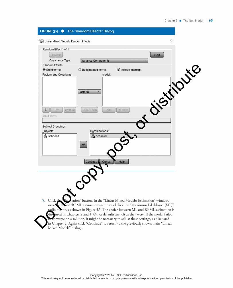
FIGURE 3.7 Fixed Effects Output in SPSS

11. RANDOM EFFECTS AND THE VARIANCE COMPONENTS/ICC TEST. In SPSS output, random effects are found in the “Estimates of Covariance Parameters” table, shown in Figure 3.8. There are two random effects, one for the between-groups school effect (labeled “Intercept[subject=schoolid]”) and one for the within-groups “Residual” effect, which reflects variance in math achievement not explained by the school effect.

FIGURE 3.8 Random Effects Output for the Null Model in SPSS

That the school variance component is significant indicates that mean math achievement varies significantly between schools. That the school component is much smaller than the residual component indicates that the majority of math achievement variation is within schools at the student level, even after controlling for the school effect.Because the null model is a variance components model, the school variance component (8.553) and the residual component (39.148) may be added together to get the total variance in math achievement (8.553 + 39.148 = 47.702). The intraclass correlation is the school component divided by the total (8.553/47.702 = 0.179). The school component is significant at the .000 level and so is the ICC since the two are mathematically equivalent in significance. Because the school variance


Do n

ot co

py, p

ost, o

r dist

ribute


component (and the ICC) is significant, the researcher concludes that multilevel modeling is necessary. Correspondingly, the researcher concludes that the estimated standard error of math achievement using OLS regression would have been in error.

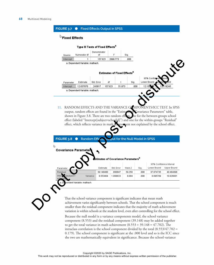
12. AIC, BIC, AND -2LL, AIC MEASURES. In SPSS, the values for -2LL, AIC, BIC, and related measures are found in the “Information Criteria” table shown in Figure 3.9. As discussed earlier in this chapter, the “-2 Log Likelihood” is the -2LL value (a.k.a. model chi-square or deviance) used as a measure of model error when conducting likelihood ratio tests discussed earlier in this chapter. Likelihood ratio tests use the -2LL value (47115.810) and model degrees of freedom (3, from the “Total” row in the “Model Dimensions” table) when comparing nested models. In Chapter 5, for example, the likelihood ratio test is illustrated to determine if a random intercept model is significantly better than the null model. For nonnested model comparisons, various information theory measures such as the Akaike information criterion (AIC) or its more conservative cousin, the Bayesian information criterion (BIC) are used. Models with lower values have less error and better fit. For a single model with no other comparison model, these measures have little use as, unlike R-squared in OLS regression, they lack an intrinsic meaning that is easily communicated.

FIGURE 3.9 -2LL, AIC, and BIC in SPSS Output


Do n

ot co

py, p

ost, o

r dist

ribute


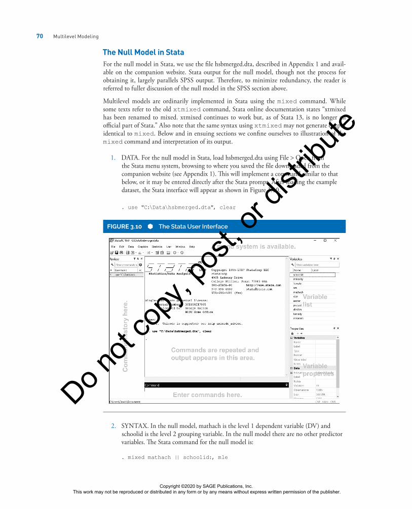
The Null Model in StataFor the null model in Stata, we use the file hsbmerged.dta, described in Appendix 1 and avail-able on the companion website. Stata output for the null model, though not the process for obtaining it, largely parallels SPSS output. Therefore, to minimize redundancy, the reader is referred to fuller discussion of the null model in the SPSS section above.

Multilevel models are ordinarily implemented in Stata using the mixed command. While some texts refer to the old xtmixed command, Stata online documentation states “xtmixed has been renamed to mixed. xtmixed continues to work but, as of Stata 13, is no longer an official part of Stata.” Also note that the same syntax using xtmixed may not generate output identical to mixed. Below and in ensuing sections we confine ourselves to illustration of the mixed command and interpretation of its output.

1. DATA. For the null model in Stata, load hsbmerged.dta using File > Open from the Stata menu system, browsing to where you saved the file downloaded from the companion website (see Appendix 1). This will implement a command similar to that below, or it may be entered directly after the Stata prompt. After loading the example dataset, the Stata interface will appear as shown in Figure 3.10.

. use "C:\Data\hsbmerged.dta", clear

FIGURE 3.10 The Stata User Interface

2. SYNTAX. In the null model, mathach is the level 1 dependent variable (DV) and schoolid is the level 2 grouping variable. In the null model there are no other predictor variables. The Stata command for the null model is:

. mixed mathach || schoolid:, mle


Do n

ot co

py, p

ost, o

r dist

ribute


The following points may be made with regard to the command syntax above:

a. mixed—This calls for linear mixed modeling, which is a synonym for multilevel modeling.

b. mathach—By being listed first, math achievement is declared to be the level 1 dependent variable.

c. || schoolid:—Random effects are set off with double bars. In the null model, only the level 2 grouping variable, schoolid, is a random effect. Random effect labels end in a colon.

d. , mle—The comma flags the start of the options list. The mle option asks for ML estimation. ML, not REML, is the default in Stata, so this option could have been omitted.

It is not necessary to request tests of random effects as this is part of default Stata output. The remaining steps interpret the output.

3. CONVERGENCE. Estimation information appears at the top of Stata output, shown below. That only two iterations are listed and no error messages appear means that convergence on a solution was reached.

Performing EM optimization:

Performing gradient-based optimization:

Iteration 0: log likelihood = -23557.905

Iteration 1: log likelihood = -23557.905

Computing standard errors:

4. DESCRIPTIVE STATISTICS AND –2LL. In the header information for default multilevel output, Stata outputs certain descriptive information along with the log likelihood (LL). This must be multiplied manually by -2 to get -2LL, which is the deviance or model chi-square value used in likelihood ratio tests when the null model is the baseline. Thus -2 * -23557.905 = 47115.810, as reported above for SPSS. Later, the researcher’s model with additional predictors should yield a significantly lower -2LL value to show less error and better fit than the null model.

Mixed-effects ML regression Number of obs = 7,185

Group variable: schoolid Number of groups = 160

Obs per group:

min = 14

avg = 44.9

max = 67

Wald chi2(0) = .

Log likelihood = -23557.905 Prob > chi2 = .

5. INFORMATION THEORY MEASURES. While -2LL is used for likelihood ratio tests when comparing nested models, information theory measures are used for nonnested as well as nested model comparisons. These measures penalize -2LL (make it higher) to compensate for the degree of complexity (lack of parsimony) in the model. In Stata, the information theory measures are not part of default output but must be requested by the postestimation command, estat ic. Only AIC and BIC are reported, but both values are the same as in SPSS above and in other packages. When comparing models, which need not be nested, lower is better model fit.


Do n

ot co

py, p

ost, o

r dist

ribute


. estat ic

Akaike’s information criterion and Bayesian information criterion

-----------------------------------------------------------------------

Model | Obs ll(null) ll(model) df AIC BIC

------------+----------------------------------------------------------

. | 7,185 . -23557.91 3 47121.81 47142.45

-----------------------------------------------------------------------

Note: N=Obs used in calculating BIC; see [R] BIC note.

6. FIXED EFFECTS. The null model has no fixed effects (level 1 regression) other than the intercept, which Stata labels “_cons” (constant). The constant is included in the level 1 fixed effects model by default. That it is significant only shows that the intercept at level 1 is significantly different from zero, which is a trivial finding. Controlling for the multilevel effect of schoolid, mean math achievement is expected to be 12.637.

-----------------------------------------------------------------------

mathach | Coef. Std. Err. z P>|z| [95% Conf. Interval]

------------+----------------------------------------------------------

_ cons | 12.63707 .2436178 51.87 0.000 12.15959 13.11455

-----------------------------------------------------------------------

7. RANDOM EFFECTS. Random effects are shown in the “Random-effects Parameters” table in Stata output, shown below. The values for the estimates are the same as in SPSS and other packages. The values in the “Estimate” column are the variance components. The “schoolid: Identity var(_cons)” row shows the component for the school effect. Since 0 is not within its confidence limits, it is significant at the .05 level. Because there is a significant school effect on mean math scores (intercepts), multilevel modeling is needed and OLS regression estimates of standard error would be in error. The “var(Residual)” row shows the residual component, reflecting within-groups (within-schools) variance in math achievement scores still unexplained after controlling for the school effect. The residual component reflects unexplained variance in the DV, which is also significant. The residual component is much larger than the variance explained by the school effect. The large unexplained (residual) effect suggests the need for a more complex model with additional predictors.

-----------------------------------------------------------------------

Random-effects Parameters | Estimate Std. Err. [95% Conf. Interval]

---------------------------+-----------------------------------------

schoolid: Identity |

var( _ cons) | 8.55352 1.068642 6.69575 10.92674

---------------------------+-----------------------------------------

var(Residual) | 39.14839 .6606469 37.87473 40.46489

-----------------------------------------------------------------------

The “Identity” part in the output above is a reminder that a diagonal covariance structure was assumed by default in Stata. In a null model, this is equivalent to a variance components structure.

8. LIKELIHOOD RATIO TEST OF THE NULL MODEL VS. OLS BASELINE. At the end of the default Stata output is the likelihood ratio test of whether the null model is significantly different from the corresponding OLS model.


Do n

ot co

py, p

ost, o

r dist

ribute


LR test vs. linear model: chibar2(01) = 983.92

Prob >= chibar2 = 0.0000

That this test is significant indicates that multilevel modeling is needed because multilevel estimates differ significantly from OLS estimates of standard errors. This test is not found in SPSS though could be computed manually. However, the variance components/ICC test serves the same function and is much more widely reported.

9. THE VARIANCE COMPONENTS/ICC TEST. A significant school effect or ICC means that a random intercept model is needed for accurate estimates. That the school variance component in random effects output above is significant is mathematically identical to finding the intraclass correlation (ICC) to be significant. The ICC is the school effect divided by the total effect, here 0.179. The significance of the ICC is mathematically identical to the significance of the school effect. By manual computation:

ICC = school effect/total effect = school effect/(school effect + residual effect)

= 8.553/(39.148 + 8.553)

= 0.179

The Null Model in SASFor the null model in SAS, we use the file hsbmerged.sas7bdat, described in Appendix 1 and available on the companion website. Because SAS output (but not input) for the null model largely parallels SPSS output, to minimize redundancy, the reader is referred to fuller discussion of the null model in previous SPSS and Stata sections in this chapter.

SAS is primarily a code-based statistical system based on input of user-supplied syntax in the (syntax) Editor window. The SAS user interface is shown in Figure 3.11.

FIGURE 3.11 The SAS User Interface


Do n

ot co

py, p

ost, o

r dist

ribute


SAS has a very large number of options within any procedure, including PROC MIXED, which is the primary SAS module used to implement multilevel models. Since this volume is aimed at the introductory graduate level, however, discussion here is restricted to core methods. The process of obtaining and interpreting null model output is given below as a series of numbered steps.

1. SYNTAX. In Figure 3.11, SAS syntax for the null model has been entered into the Editor window shown at the bottom. When viewed on a monitor the start and end of a SAS procedure is shown in black (here, PROC MIXED. . . .RUN). Other SAS command words and options are shown in blue. Note that statements end in semi-colons. Options for a statement are delimited by a slash mark. In this figure, the syntax has already been run so output is shown in the “Results Viewer” window above the syntax editing window. Also, in the “Results” window on the left, a table of contents to sections of the results is available. SAS has other windows, some of which have tabs shown at the bottom of Figure 3.11, for additional types of information. For instance, error messages appear in the Log window.

Below is the commented SAS syntax needed to generate output for the null model, parallel to the previous sections for SPSS and Stata. Comments are shown in green, within “/*. . . */” markers. Comments are ignored by SAS, being only for the reader’s benefit.

LIBNAME in "C:\Data";

/* LIBNAME sets a pointer with the user-supplied name "in"*/

/* which points to the data directory, differs for */

/* each user. */

TITLE "Multilevel Null Model";

/* TITLE puts a heading on each output page */

PROC MIXED DATA=in.hsbmerged COVTEST METHOD = ML;

/* PROC MIXED invokes SAS’s multilevel modeling module */

/* DATA= specifies the data file to use; the .sas7bdat */

/* extension is assumed */

/* COVTEST requests tests of random effects */

/* METHOD = ML overrides SAS’s default of REML estimation */

CLASS schoolid;

/* CLASS declares schoolid as a categorical variable,*/

/* which the Level 2 grouping variable must be */

MODEL mathach = /SOLUTION CL;

/* mathach is declared the Level 1 dependent variable */

/* /SOLUTION asks for fixed effects output. */

/* In the null model there are no level 1 fixed effects */

/* except the level 1 intercept, which is included by */

/* default unless the NOINT option is included */

/* CL causes display of fixed effects confidence limits */


Do n

ot co

py, p

ost, o

r dist

ribute


/* In more complex models, the MODEL statement is where */

/* fixed effects are listed. */

RANDOM INTERCEPT / SUBJECT=schoolid CL;

/* The RANDOM statement lists random effects */

/* In null models, only the intercept is a random effect */

/* INTERCEPT requests a level 2 intercept be included in /*

/* the model as a random effect */

/* SUBJECT= declares schoolid to be the level 2 grouping /*

/* variable */

/* CL causes display of random effects confidence limits */

RUN;

/* Runs the model. */

After entering the syntax above (possibly without comments) into the syntax editing win-dow, the “Run” icon at the top of the user interface is clicked to actually run the model. This is necessary even though “RUN;” is part of the syntax. This icon looks like a running person. Alternatively, one may select “Run” from the main menu at the top, also shown in Figure 3.11. Output is discussed in subsequent steps.

2. CONVERGENCE. If convergence is reached satisfactorily, SAS states so, as shown at the bottom of the iteration history in Figure 3.12.

FIGURE 3.12 The SAS Iteration History for the Null Model

3. MODEL INFORMATION. Model information in the initial portion of SAS output simply reminds the researcher of the input and model specifications, including that mathach is modeled under ML estimation using a variance components covariance structure assumption. There are 160 schools (schoolids are shown in the “Class Level Identification” table) and 7,185 students, as shown in Figures 3.13A and 3.13B.


Do n

ot co

py, p

ost, o

r dist

ribute


FIGURE 3.13A Model Information for the Null Model in SAS

FIGURE 3.13B Dimensions and Number of Observations in SAS


Do n

ot co

py, p

ost, o

r dist

ribute


4. FIT STATISTICS AND -2LL. As shown in Figure 3.14, in the “Fit Statistics” table, SAS reports -2 log likelihood (-2LL), which is the deviance or model chi-square value used in likelihood ratio tests when the null model is the baseline.

FIGURE 3.14 Information Theory Measures and -2LL for the Null Model in SAS

5. INFORMATION THEORY MEASURES. Also in Figure 3.14, SAS reports the Information theory measures AIC, AICC, and BIC, all of which penalize -2LL (make it higher) to compensate for the degree of complexity (lack of parsimony) in the model. Later, when comparing models, which need not be nested, lower is better model fit. Here, corrected AIC (CAIC) is identical to AIC, whereas it can be seen that BIC has a more conservative (higher) value. Note that SAS uses a different formula for BIC. Whereas the default for sample size in the BIC formula is the level 1 sample size in SPSS, Stata, and R, it is the level 2 sample size in SAS. This difference in formulas will not matter as long as the researcher uses BIC as output by the same statistical package for all model comparisons.

6. FIXED EFFECTS. SAS reports level 1 fixed effects, also known as the regression model, in the “Solution for Fixed Effects” table in Figure 3.15. The only fixed effect in the null model is the level 1 intercept since there are no predictor variables. That the intercept (constant) term is significant trivially shows that the intercept is significantly different from zero.

FIGURE 3.15 Fixed Effects for the Null Model in SAS

7. RANDOM EFFECTS. Random effects are shown in the “Covariance Parameters Estimates” table in SAS output, shown in Figure 3.16. The values for the estimates are the same as for other packages.


Do n

ot co

py, p

ost, o

r dist

ribute


• The “Intercept” random effect is the school effect, reflecting between-school variance in mathach. The “Pr > Z” column on the right shows that the school effect is significant. This implies that a multilevel model is needed to properly estimate effects in a random intercepts model and that OLS estimates would be in error.

• The “Residual” random effect row reflects within-group variance in mathach remaining after the school effect is controlled. That it is much larger than the variance component explained by the school effect means that there is much unexplained variance in the null model, which is typical. Therefore, there is reason to proceed with a more complex model involving additional predictors at level 1 and/or additional predictors and random effects at level 2 or higher.

FIGURE 3.16 Random Effects for the Null Model in SAS

8. THE VARIANCE COMPONENTS/ICC TEST. That the school variance component is significant is mathematically identical to finding the intraclass correlation (ICC) to be significant. Both indicate there is significant between-schools variation in math achievement due to the nonindependence (clustering) of math scores by school. The ICC is the school effect divided by the total effect, as in the formula below.


= 8.5490/(39.1488 + 8.5490)

= 0.179

The multilevel modeling algorithm runs one regression for each of the 160 schools in the level 2 sample. Variation in the estimated intercepts of these 160 equations is used to adjust estimates of the standard error of the intercept (reflecting mean math score) at level 1. In the “Solution for Random Effects” table, not shown here due to length, SAS prints out the intercept estimates for each of the 160 regression equations. While this table is rarely reported in multilevel articles, it is helpful in providing insight into the process of multilevel modeling.

The Null Model in HLM 7For the null model in HLM 7, we use as input the SPSS-format file hsbmerged.sav, described in Appendix 1 and available on the companion website. HLM 7 output largely parallels SPSS output for the null model. Therefore to minimize redundancy, the reader is referred to fuller discussion of the null model in the SPSS section and other earlier sections of this chapter. The HLM 7 user inter-face, however, is quite different, involving creation of special files unique to HLM 7 (.mdmt, .mdm; both are also available at the companion website). In later chapters, the reader may wish to refer back to the HLM 7 section of Chapter 3 to recall the process for creating .mdmt and .mdm files.


Do n

ot co

py, p

ost, o

r dist

ribute


HLM 7 is authored by three leaders in the field of multilevel modeling, Stephen Raudenbush and Anthony Bryck (2002) and Richard Congdon, along with their associates. The manual is Raudenbush, Bryk, Cheong, Congdon, and Du Toit (2011). Software, including a free student version, is available from Scientific Software International (SSI, www.ssicentral.com). The stu-dent version will support the example data file used here.

To obtain the null model in HLM7, we follow the steps enumerated below. The earlier steps create the “multivariate data matrix template” (.mdmt) file which is used in a later step, to create the “multivariate data matrix” (.mdm) file for a particular model, in this case the null model. The .mdmt file defines a dataset and variables to be used in possibly multiple models while the .mdm file uses the .mdmt file to create a file specific to a given model such as the null model.

1. CREATING THE MDM FILE. The first step in multilevel analysis with HLM 7 is to declare the data file and variables of interest, including the grouping (link, level) variables defining levels in the analysis. In doing this we create a .mdm file, which stands for “multivariate data matrix file” and which is a data file in HLM 7 format. Later in the process of creating the .mdm file, the “multivariate data matrix template” (.mdmt) file will also be created so it may be used as a template which can be reused for a variety of multilevel models, including the null model.

Run HLM 7 and select File > Make new MDM file > Stat package input, arriving at the initial HLM 7 page as shown in Figure 3.17. While the menu provides for reading data from a text file, in this exercise we select “Stat package input” and proceed to load the SPSS-form file, hsbmerged.sav, used earlier in the SPSS section.

FIGURE 3.17 HLM 7 File Menu


Do n

ot co

py, p

ost, o

r dist

ribute


2. In the “Select MDM type” dialog which opens, select the desired type of multilevel model. For this example we request the two-level hierarchical linear model, HLM2, as shown in Figure 3.18. Then click OK.

FIGURE 3.18 HLM 7 Select MDM Type Window

Figure 3.18 lists various types of models which may be run with HLM 7 software:

• HLM2 is for two-level hierarchical (nested) models.• HLM3 is for three-level hierarchical models.• HLM4 is for four-level hierarchical models.• HMLM models are for hierarchical multivariate linear models, meaning ones with

more than one dependent variable.• HMLM2 models are ones with multiple dependent variables such as ones where level

1 measures are nested within persons and persons are nested with some higher level.• HCM2 models are ones in which level 1 units (e.g., students) are cross-classified by

two higher level factors, such as neighborhoods and schools. In a hierarchical model, students would be listed by school and schools would be listed by neighborhood (assuming multiple schools per neighborhood). In a cross-classified model, where students in a given neighborhood may attend more than one school and a given school might recruit from more than one neighborhood, students are listed in cells formed by a matrix in which schools may be rows and neighborhoods may be columns. Cross-classified models are treated in Chapter 11.

• HCM3 is for three-level hierarchical and cross-classified models. In this type of model, students are listed in cells in the neighborhood-vs-school matrix as in HCM2, but columns (e.g., neighborhoods) may be clustered within a higher level such as municipalities.

• HLM-HCM is for hierarchical linear models with level 2 units cross-classified at level 3. An example would be repeated measures nested within students at level 2, with students cross-classified by a matrix in which rows are neighborhoods and schools are columns.


Do n

ot co

py, p

ost, o

r dist

ribute


3. After selecting the model type, the “Make MDM” dialog window appears, shown in Figure 3.19. Highlights have been added to show the entries for the current example.

FIGURE 3.19 The HLM2 Make MDM Page

Note in the “Level-1 Specification” and “Level-2 Specification” areas of Figure 3.19 that HLM 7 can read SPSS .sav files. Other possible formats include SAS transport files, Stata files, and Systat files. Warning: it is essential that the data files be sorted by the level 2 grouping (link) variable, which is schoolid in this example. This has already been done in the downloadable example file provided. The researcher must also declare whether or not level 1 data rows have missing data, or must elect how to delete rows with missing data. The example dataset does not have missing data. Note here that the same datafile, hsbmerged.sav, is listed for both the level 1 data and the level 2 data. It is, however, possible to have each level in a separate file if desired.

4. Still on the “Make MDM” page, click the “Choose Variables” button for level 1, leading to the window shown in Figure 3.20. In the first (ID) column, check schoolid as the level 2 grouping variable which links level 1 to level 2. In the other column, check other level 1 (student level) variables to be used in the researcher’s models even if not needed for the null model. One of these must be the dependent variable, here mathach (math achievement score). Here, the level 1 variables mathach, minority, female, and ses are checked. Click OK to return to the “Make MDM” window.


Do n

ot co

py, p

ost, o

r dist

ribute


5. On the “Make MDM” page, click the “Choose Variables” button for level 2 as shown in Figure 3.21. In the first (ID) column, again check schoolid as the level 2 link variable. In the other column, check other level 2 (school level) variables to be used in the researcher’s models even if not needed for the null model. These are size through meanses in Figure 3.21. Click OK to return to the “Make MDM” window.

FIGURE 3.20 The HLM2 Level 1 Choose Variables Window

FIGURE 3.21 The HLM2 Level 2 Choose Variables Window


Do n

ot co

py, p

ost, o

r dist

ribute


6. Also on the “Make MDM” page, click the “Save mdmt file” button near the top and save to the desired directory with the desired filename (e.g., hsbmerged.mdmt), as shown in Figure 3.22. The .mdmt file is an MDM template file which can be retrieved to implement a variety of models using the data file and variables named in steps above.

FIGURE 3.22 HLM 7 Save MDM Template Window

FIGURE 3.23 Null Model Descriptive Statistics

7. Click the “Make MDM” button at the bottom of the “Make MDM” page shown in Figure 3.19. HLM 7 pops up a page of descriptive statistics, shown in Figure 3.23.


Do n

ot co

py, p

ost, o

r dist

ribute


8. Click the “Done” button on the “Make MDM” page shown in Figure 3.19. The foregoing steps created hsbmerged.mdmt, a template file which may be used to create a variety of multilevel models using the dataset and variables selected above. In the next set of steps, a model is created for a specific model, in this case the two-level null model with mathach as the dependent variable at level 1 and schoolid as the grouping (link) variable at level 2.

9. Upon clicking “Done” in the previous step, the window shown in Figure 3.24 appears. Here the researcher may specify the null model. Specify mathach as the level 1 dependent variable. The researcher is given the ability to specify that mathach should be entered uncentered, group centered, or grand mean centered. Here we choose uncentered, in order to follow Raudenbush and Bryck (2002). In a null model there are no other level 1 variables. Note the arrows (“>>” and “<<”) show what level of the model you are dealing with at any given moment. Here the level 1 variables are listed.

FIGURE 3.24 HLM 7 DV Selection Window

10. Upon entering mathach as the level 1 dependent variable, HLM 7 displays the model selected thus far, in equation form, as shown in Figure 3.25. Because

“>>Level-2<<” is selected on the left-hand size, level 2 variables are shown, but this does not affect computation. Note it is not necessary to specify schoolid as the level 2 grouping (link) variable as that was done when the .mdmt file was created in a previous step.

The level 1 model equation is read as “MATHACH is a function of a level 1 intercept term plus level 1 residual error.” The level 2 model is read as “The level 1 intercept term equals the grand mean of intercepts at level 2 plus a random error term (which indicates the intercept is modeled as a random effect).” Some researchers find the explicit statement of the operational equation at each level of analysis to be an aid to understanding the model and an advantage of HLM 7.


Do n

ot co

py, p

ost, o

r dist

ribute


11. Before running the null model above, settings should be checked. First click “Basic Settings” in the dialog shown in Figure 3.25. As shown in Figure 3.26, declare the distribution of mathach to be normal/continuous. Other distribution choices are discussed in Chapter 12, which deals with generalized multilevel models. In the “Basic Model Specifications” window, also give a title and an output filename for the model being created. Click OK when done.

FIGURE 3.25 HLM 7 Models Window

FIGURE 3.26 HLM2 Model Specifications Window


Do n

ot co

py, p

ost, o

r dist

ribute


12. Then select “Other Settings > Estimation Settings” from the modeling window. Override HLM 7’s default REML estimation method and replace it with ML as shown in Figure 3.27. There are many other settings here, some of which the text will come back to, but this is the only one needed for the null model. Click OK to return to the modeling window.

FIGURE 3.27 HLM2 Estimations Settings Window

13. Then select “Other Settings > Output Settings” from the modeling window. As shown in Figure 3.28, change settings as desired. In the current example, two defaults are overridden: (1) check to print the variance-covariances matrices and (2) uncheck “Reduced output” so as to get full output. Click OK to return to the modeling window.

FIGURE 3.28 HLM 7 Output Settings Window


Do n

ot co

py, p

ost, o

r dist

ribute


14. Select File > Save As to save the model under a name such as “Null_Model.” This creates a command file called Null_Model.hlm and an output file called Null_Model .html. Retain the files created here in the null model section as they will be used in later chapters.

15. From the HLM2 modeling window, select “Run Analysis” to obtain the output discussed in the numbered sections below. As the output is a .html file, it will appear in the browser, not in HLM 7 itself.

16. MODEL INFORMATION. Null model output is shown below in Courier New font. The initial “Specification for this HLM2 run” section reminds us that we are using the previously specified “hsbmerged” data in a model we have named “Null_Model.” There are 7,185 students at level 1 and 160 schools at level 2. We are using full maximum likelihood estimation. Though the default covariance structure in HLM 7 is unstructured (UN) rather than variance components, this will not matter for the estimates discussed below since the null model is a type of random intercept model. Estimates conform to those in SPSS, SAS, and Stata.

Specifications for this HLM2 run

Problem Title: Null _ Model

The data source for this run = hsbmerged.mdm

The command file for this run = C:\Multilevel\Null _ Model.hlm

Output file name = C:\Multilevel\Null _ Model.html

The maximum number of level-1 units = 7185

The maximum number of level-2 units = 160

The maximum number of iterations = 100

Method of estimation: full maximum likelihood

17. MODEL SUMMARY. The model summary section of output shows the model in equation form. For the null model, at level 1, MATHACH is equal to an intercept and a residual error term. The intercept, β0j, is a function at level 2 of the mean of all 160 intercepts (γ00) plus a random error term (u0j). The “mixed model” equation is an equivalent mathematical integration of the level 1 and level 2 equations.

The outcome variable is MATHACH

Summary of the model specified

Level-1 Model

MATHACHij = β

0j + r

ij

Level-2 Model

β0j = γ

00 + u

0j

Mixed Model

MATHACHij = γ

00 + u

0j+ r

ij

18. FIXED EFFECTS (INITIAL). By default, HLM 7 first presents the level 1 regression model both for OLS estimates and for multilevel estimates using the requested method, ML. OLS estimates are presented without and then with robust standard errors. The multilevel intercept estimate, shown under the heading “Estimation of fixed effects,” is 12.64, as in SPSS, SAS, and Stata. The robust OLS estimate is inflated somewhat (12.74). Note, however, these are estimates based on starting values. A refined set of estimates follows the iteration process and convergence on a solution in the next step.


Do n

ot co

py, p

ost, o

r dist

ribute


Initial results

The average OLS level-1 coefficient for INTRCPT1 = 12.62075

Least Squares Estimates

σ2 = 47.30368

Least-squares estimates of fixed effects

Fixed Effect Coefficient

Standard

error t-ratio

Approx.

d.f. p-value

For INTRCPT1, β0

INTRCPT2, γ00

12.747853 0.081140 157.110 7184 <0.001

Least-squares estimates of fixed effects

(with robust standard errors)


Standard

error t-ratio

Approx.

d.f. p-value

For INTRCPT1, β0

INTRCPT2, γ00

12.747853 0.239305 53.270 7184 <0.001

Starting Values

σ2(0) = 39.14163

τ(0)

INTRCPT1,β0

8.72185

Estimation of fixed effects

(Based on starting values of covariance components)


Standard

error t-ratio

Approx.

d.f. p-value

For INTRCPT1, β0

INTRCPT2, γ00

12.636803 0.245768 51.418 159 <0.001

19. CONVERGENCE. Following the fixed effects model, HLM 7 prints out iteration history. It shows that convergence on a solution was reached after four iterations. A refined set of fixed effects output follows the iterations history. Differences from the starting values estimates are very small for the data at hand.

The value of the log-likelihood function at iteration 1 = -2.355710E+004



Final Results - Iteration 4

Iterations stopped due to small change in likelihood function

σ2 = 39.14838

Standard error of σ2 = 0.66054

τ

INTRCPT1, β0 8.55379

Standard error of τ

INTRCPT1, β0 1.06124


Do n

ot co

py, p

ost, o

r dist

ribute


Random level-1

coefficient

Reliability estimate

INTRCPT1,β00.901


Final estimation of fixed effects:


Standard

error t-ratio

Approx.

d.f. p-value

For INTRCPT1, β0

INTRCPT2, γ00

12.637067 0.243638 51.868 159 <0.001

Final estimation of fixed effects

(with robust standard errors)


Standard

error t-ratio

Approx.

d.f. p-value

For INTRCPT1, β0

INTRCPT2, γ00

12.637067 0.243617 51.873 159 <0.001

20. RANDOM EFFECTS. Random effects appear in the “Final estimation of variance4 components” table, shown below. HLM 7 labels the intercept effect, which is the between-groups school effect on math achievement at level 1, as “INTRCPT1, u0.” It labels the within-groups residual effect as “level-1, r.” The residual effect reflects variance in math achievement after the school random effect is controlled. That it is much larger than the school effect suggests the need for better specification of the model.

Final estimation of variance components

Random Effect

Standard

Deviation

Variance

Component d.f. χ2 p-value

INTRCPT1, u0

2.92469 8.55379 159 1660.22552 <0.001

level-1, r 6.25687 39.14838

21. THE VARIANCE COMPONENTS/ICC TEST. That the p value for the school (intercept) effect is significant means that the clustering of math achievement scores by schoolid is significant and will affect estimates of mean math achievement at level 1. This also means OLS estimates will be in error compared to multilevel estimates. The significance of ICC is mathematically identical to the significance of the school effect above. The ICC is the school effect divided by the total effect, here 0.179.


= 8.55379/(39.14838 + 8.55379)

= 0.179

22. MODEL CHI-SQUARE/DEVIANCE (-2LL). At the bottom of output, HLM 7 prints the deviance, which is a -2 log likelihood measure commonly used as the


Do n

ot co

py, p

ost, o

r dist

ribute


baseline in likelihood ratio tests discussed earlier in this chapter. The estimate in HLM is trivially different from that in SPSS, SAS, and Stata due to minor algorithmic differences (47113.97 in HLM 7 compared to 47115.81 in other packages).

Statistics for the current model

Deviance = 47113.972333

Number of estimated parameters = 3

23. INFORMATION THEORY MEASURES. Where -2LL is used for comparing nested models, information theory measures like AIC and BIC are commonly used to compare nonnested as well as nested models. HLM 7 does not output information theory measures though they may be computed manually as described in Online Appendix 2.

24. SAVED MATRICES. By default, HLM 7 saves certain matrices to file, noted in a final section of output shown below. These matrices, particularly the tau matrix, may be examined in the event of failure to converge on a solution, looking for variance components close to 0, collinearity among random effects, or, in the gamma matrix, extreme estimates in the level 1 regression.

tauvc.dat, containing tau and the variance-covariance matrix of tau

has been created.

The file tauvc.dat contains the variance-covariance matrix associated with random effects. In general, tauvc.dat contains tau(pi); tau(beta); and the inverse of the information matrix. It has these contents for the current example:

• 8.5537872 (variance component for the school effect on the intercept of mathach, labeled as σ2

(0) by HLM7)

• 1.1262391 (This is the square of the standard error of tau, which in HLM 7 output is labeled “Standard error of τ, INTRCPT1,β0).” Squared standard error, of course, is variance.

• 39.1483812 (variance component for the residual effect, labeled τ(0) INTRCPT1,β0 )

• In this equivalent to a variance components model, the covariance between the two random effects is 0 and is not shown in tauvc.dat.

gamvc.dat, containing the variance-covariance matrix of gamma has

been created.

The file gamvc.dat contains the variance-covariance matrix associated with fixed effects. The gamvc.dat file contains the nonrobust version of the gamma values and the gamma variance- covariance matrix used to compute the robust standard errors. For instance, this file contains the intercept fixed effect, previously computed to be 12.6370672 and labeled “INTRCPT1, β0 INTRCPT2, γ00” in HLM 7.

gamvcr.dat, containing the robust variance-covariance matrix of gamma has

been created.

The gamvcr.dat file contains the robust version of the gamma values and the gamma variance- covariance matrix used to compute the robust standard errors.


Do n

ot co

py, p

ost, o

r dist

ribute


The Null Model in RFor the null model in R, we use the file hsbmerged.rds, described in Appendix 1 and available on the companion website. The process for importing data from other packages is described in Online Appendix 1. For this exercise we import hsbmerged.sav, which is in SPSS format. For anal-ysis we use the R package called lme4, which currently is the most widely used one for multilevel modeling in R (Hox, Moerbeek, & van de Schoot, 2018, p. 25; Bates, 2010; Bates et al., 2015).

R syntax for the null model

# LOAD AND VIEW THE DATA# Set the working directorysetwd("c:/Multilevel")

# Clear the environment of previous datarm(list=ls())

# Assuming the haven package has been installed, invoke it# Otherwise type install.packages(“haven”)

library(haven)

# Read data from an SPSS format file into the object hsbmergedhsbmerged <- read _ sav("hsbmerged.sav")

# Optionally, view the data (capitalize "View")View(hsbmerged)

# NULL MODEL WITH lmer() FUNCTION FROM PACKAGE LME4# If not yet installed, install the lme4 linear modeling package# with the command as in Online Appendix 1: install.packages("lme4")# The lme4 package supports the lmer() multilevel model functionlibrary(lme4)

# Run the null model using ML estimationNullModel <- lmer(mathach~(1|schoolid), REML = FALSE, data = hsbmerged)

# View the outputsummary(NullModel)

Comments on lmer() syntax for the null model:NullModel <- lmer(mathach~ (1|schoolid), REML = FALSE, data = hsbmerged)

NullModel <-

Output is sent to an object called NullModellmer(mathach

Multilevel modeling is invoked with mathach as dependent variable~(1|schoolid)

Predictors are listed after the tilde. Here there is only the random schoolid effect.Level 1 observations are nested within schoolid at level 2.Note a random effect is enclosed in parentheses. If there were more than onerandom effect, they would be separated by a double vertical bar (||).

,

A comma separates the list of options


Do n

ot co

py, p

ost, o

r dist

ribute


REML = FALSE,

REML estimation is the default. Setting it to FALSE invokes maximum likelihood(ML) estimation.

data = hsbmerged)

The dataset data frame hsbmerged is named as the data source.summary(NullModel)

The separate summary command displays the output. It must be lower case. This command is unnecessary if the entire command string is enclosed within parentheses, thereby causing output to appear automatically:

Output from the lmer() procedure

Output coefficients are the same as in other statistical packages previously discussed in this chapter:

NullModel <- lmer(mathach~ (1|schoolid), REML = FALSE, data = hsbmerged)

summary(NullModel)

Linear mixed model fit by maximum likelihood [’lmerMod’]

Formula: mathach ~ (1 | schoolid)

Data: hsbmerged

AIC BIC logLik deviance df.resid

47121.8 47142.4 -23557.9 47115.8 7182

Scaled residuals:

Min 1Q Median 3Q Max

-3.06262 -0.75365 0.02676 0.76070 2.74184

Random effects:

Groups Name Variance Std.Dev.

schoolid (Intercept) 8.553 2.925

Residual 39.148 6.257

Number of obs: 7185, groups: schoolid, 160

Fixed effects:

Estimate Std. Error t value

(Intercept) 12.6371 0.2436 51.87

Interpretation of outputBecause R output (but not input) for the null model largely parallels output from previously discussed packages, to minimize redundancy the reader is referred to fuller discussion of the null model in the SPSS and other earlier sections of this chapter.

1. SIGNIFICANCE COEFFICIENTS (p VALUES). Casual inspection of R output above shows the lmer()procedure does not output significance coefficients for either fixed or random effects. However, t values are output for fixed effects and standard deviations are output for random effects. This omission is not an accident but rather reflects the view of the author of the lme4 package that what is a true “p” parameter


Do n

ot co

py, p

ost, o

r dist

ribute


is a matter of dispute since the usual t-distribution method does not always yield correct p-value estimates, leading the author to not include p values in the lmer() function.1 A preferred way of significance testing is using the likelihood ratio test of the difference between two models, such as between one with and one without a given variable or effect. This is illustrated in Chapter 4 but cannot be illustrated here since there is only the one model (the null model). Alternatively, p values may be estimated using the lmerTest package, as described further below in the section on random effects output. (Note that the Monte Carlo approach to obtaining p values described by Finch, Bolin, and Kelley, 2014, pp. 57–59, no longer works with the lmer() function.2 )

2. CONVERGENCE. If the null model discussed here were run under REML estimation (using the REML = TRUE) option, then if convergence is satisfied, output will include this line:

REML criterion at convergence: 47116.79

If ML estimation is used, as in the example in this chapter, there is no corresponding output line. In the example illustrated above, convergence was achieved. Failure to converge would lead to an error message such as the following:

Model failed to converge: degenerate Hessian with 1 negative eigenvalues

3. MODEL INFORMATION. Basic model information appears at the top of R output, showing math achievement was modeled as an effect of the level-2 grouping variable schoolid, using ML estimation based on the hsbmerged dataset.

Linear mixed model fit by maximum likelihood [’lmerMod’]

Formula: mathach ~ (1 | schoolid)

Data: hsbmerged

Below the random effects output, it is noted that there are 7,185 students grouped in 160 schools.

Number of obs: 7185, groups: schoolid, 160

4. FIT STATISTICS, -2LL, AND INFORMATION THEORY MEASURES. In R output below, -2LL is labeled “deviance” and is -2*logLik. This value is used when comparing nested models using the likelihood ratio test. The AIC and BIC information criteria are also listed, used for comparing unnested as well as nested models, where lower is less error and better fit.

AIC BIC logLik deviance df.resid

47121.8 47142.4 -23557.9 47115.8 7182

5. FIXED EFFECTS. Fixed effects are the regression part of the model and interpreted as such. Controlling for other effects in the model (the only one of which is the effect of the level 2 grouping variable, schoolid) the intercept of 12.6371 is the estimate of the mean mathach score. While significance coefficients (p values) are not displayed, that the estimate is more than 1.86 standard errors from 0 means it is significant at better than the .05 level. The 5% confidence limits on the estimate are +/- 1.96*0.2436.


Do n

ot co

py, p

ost, o

r dist

ribute


Fixed effects:

Estimate Std. Error t value

(Intercept) 12.6371 0.2436 51.87

Note that unlike the lmer() function in the lme4 package discussed here, the lme() multi-level modeling command in the nmle package, though now considered outdated by some, does generate fixed effects p values (though not random component p values). See Online Appendix 1.

6. RANDOM EFFECTS. In the null model there are two random effects: the school effect based on schoolid as the level 2 grouping variable, and the residual effect. These are the between-groups and within-groups effects respectively. Again, p values are not displayed. The standard deviations are no standard errors and cannot be used directly to compute confidence limits around the random effect components, similar to what was done for fixed effects.

Random effects:

Groups Name Variance Std.Dev.

schoolid (Intercept) 8.553 2.925

Residual 39.148 6.257

The needed p values can be generated using the lmerTest package, whose rand() function gives a p value for the variance component of a grouping variable in a null model, such as for the previously created object NullModel, whose grouping variable was schoolid. Later, for more complex models, the summary() and anova() commands lmerTest will also give p val-ues. Click the “Install” icon under the “Packages” tab in RStudio, then enter lmerTest as the package to install. A large number of subsidiary packages will also be installed. In RStudio, check the box for the lmerTest package, equivalent to issuing a library() command. Below we invoke the lmerTest library, re-create NullModel using the same formula as before, then run the rand() command. It shows that the schoolid effect is significant at better than the 0.001 level (p approximates .000, as in other statistical packages). Use of lmerTest is illustrated more fully in Chapter 6.

library(lmerTest)

NullModel <- lmer(mathach~(1|schoolid), REML = FALSE, data = hsbmerged)

rand(NullModel)

Analysis of Random effects Table:

Chi.sq Chi.DF p.value

schoolid 986 1 <2e-16 ***

---

Signif. codes: 0 ‘***’ 0.001 ‘**’ 0.01 ‘*’ 0.05 ‘.’ 0.1 ‘ ’ 1

7. VARIANCE COMPONENTS/ICC TEST. The intraclass correlation is the schoolid component divided by the sum of both components:

ICC = 8.553/(8.553 + 39.148) = 0.179

Since the schoolid random effect component was significant, we can say that the ICC (which is mathematically equivalent) is also significant. For either, significance indicates the need for multilevel modeling and that OLS estimation would be in error.


Do n

ot co

py, p

ost, o

r dist

ribute


Summary

Key concepts learned by the reader in Chapter 3 include the following points:

• The primary purpose of the null model is to test whether the values of the dependent variable (DV) at level 1 cluster within groups formed by the grouping (level) variable at level 2, thereby violating the data independence assumption of OLS regression and indicating the need for multilevel modeling.

• When the data independence assumption of OLS regression is violated, estimates of standard errors will be wrong and significance tests will not be accurate.

• A secondary purpose of the null model is to serve as a baseline of comparison with later models.

• Comparison of models is accomplished through the likelihood ratio test, which is based on -2LL, also known as the model chi-square or deviance value.

• The deviance value is a measure of error, with lower being less error and better model fit.

• Likelihood ratio tests assume that the smaller model is nested within the larger model. For nonnested comparisons, information theory measures such as AIC or BIC are used.

• The Wald test is an alternative to the likelihood ratio test and is available in some packages such as SPSS. In general, the likelihood ratio test is preferred.

• When fixed effects differ between models being compared, ML rather than REML estimation should be used. Most statistical packages default to REML and therefore ML must be requested explicitly if it is desired.

• The fixed effects portion of the null model includes only the intercept and is of only minor research interest.

• The random effects portion of the null model includes two effects. The random effect of

the level 2 grouping variable is the between-groups effect, reflecting variation in the mean of the level 1 DV across groups. The other random effect is the residual effect, reflecting the within-group variation in the DV after the random effect of the level 2 grouping variable is controlled. The residual effect thus represents unexplained variance in the DV.

• The label for the random effects table varies by statistical package used. Common labels are the variance components, covariance parameters, or random effects table.

• The intraclass correlation (ICC) is calculated as the variance component of the grouping variable divided by the sum of both variance components (both the residual component plus the grouping variable component). If the grouping variable component is significant, then the ICC will be significant. In either of these mathematically equivalent cases, significance indicates the need for multilevel modeling. This is called the “ICC test.”

• While it is widely stated that the ICC test presumes that the researcher has specified a variance components (VC) variance-covariance structure, the specification of a variance-covariance structure is ignored for random intercept models (ones where only the intercept is modeled, not any slopes). The null model is a type of random intercept model.

• The ICC test may lead to different results than an ANOVA test of the same DV and grouping variable. This is because they test different things.

• In any statistical package, results should not be reported unless convergence on a solution has been achieved.

• Difference among statistical packages are illustrated by differences in default output for information theory fit statistics. Stata and R generate AIC (the Akaike information criterion) and BIC (Bayes information criterion).


Do n

ot co

py, p

ost, o

r dist

ribute


SAS generates AIC, BIC, and AICC (corrected AIC, used when sample size is small). SPSS generates AIC, BIC, AICC, and CAIC (consistent AIC, an alternative to AICC, used to penalize for lack of parsimony in small samples). HLM 7 does not generate any of these, though manual computation is possible.

• HLM 7 shows equations for each level and each intercept or slope effect. The other packages use a single-equation model. HLM 7 is also the only package which by default generates reliability coefficients. Likelihood ratio tests are a built-in function in HLM 7. HLM 7 by default outputs both ordinary and robust estimates, though robust standard error models are easily

implanted in Stata, and with less ease, in other packages.

• Stata by default outputs a likelihood ratio test of the difference between the OLS model and the multilevel model.

• For multilevel modeling, the main SPSS module is the MIXED module. For Stata, the main multilevel command is the mixed command. For SAS, the main multilevel analysis module is PROC MIXED. HLM 7 has eight multilevel analysis modules. The one used in this chapter for the null model was HLM2. The leading packages in R for multilevel analysis are the lme4 and the lmerTest packages, with the latter requiring the former.

Glossary

ANOVA F-testAnalysis of variance (ANOVA) relies on F-tests of signif-icance of differences among group means. The ANOVA F-test is a function of the variance of the set of group means, the overall mean of all observations, and the variances of the observations in each group weighted for group sample size. The larger the difference in means, the larger the sample sizes, and/or the lower the vari-ances, the more likely ANOVA results will be significant. The output may be labeled the ANOVA table, the variance components table, the covariance parameters table, or the random effects table, depending on what software package is used.

Assumption of independenceA critical assumption of ordinary least squares (OLS) regression, the independence assumption requires data to be independent. In the context of multilevel model-ing, when the values of the dependent variable at level 1 cluster within groups formed by the grouping (level) variable at level 2, the OLS assumption of independence is violated.

If OLS regression is used despite a violation of the independence assumption, estimates of standard errors will be wrong and significant tests will not be accurate.

Information theory fit statisticsIn likelihood ratio testing, -2LL (model chi-square, devi-ance) is a measure of model error, with lower repre-senting better model fit. Information theory fit statistics penalize -2LL to adjust for lack of parsimony. Where likelihood ratio testing is appropriate for comparing nested models, information theory measures are used to compare either nested or nonnested models, again with lower representing better fit. Common information theory fit measures include the Akaike information cri-terion (AIC) and the Bayesian information criterion (BIC). Of these, BIC is the more conservative measure, penal-izing lack of parsimony more heavily.

Intraclass correlation (ICC)The intraclass correlation (ICC) is the share of variance accounted for by the random effect of the intercept com-ponent in a null model. As the null model contains no other random or fixed effects, in a two-level model the ICC reflects the effect size of the level 2 grouping vari-able. Finding a significant ICC based on the grouping variable indicates multilevel modeling is needed, as the level 1 DV is not independent of the level 2 grouping vari-able. If in a null model the intercept component is sig-nificant, then the ICC will also be significant. If either is nonsignificant, OLS regression may be appropriate and multilevel model not needed.


Do n

ot co

py, p

ost, o

r dist

ribute


Likelihood ratio testWhen using maximum likelihood estimation (ML), as is typical in multilevel modeling, output includes the effect size measure of likelihood (L). When the log is taken of this value and then multiplied by negative 2, the result is the -2LL statistic, also called model chi square or devi-ance. The -2LL statistic conforms to a chi-square dis-tribution, allowing it to be used for significance testing. The likelihood ratio test (a.k.a. chi-square difference test) utilizes this -2LL value to test the amount of error in a given model comparison to another version of the model. The smaller model must be nested within the larger model. In general, the likelihood ratio (LR) test assesses whether the researcher’s model has signifi-cantly less error and hence better fit than the null model, but other bases of comparison than the null model are also possible.

Nested models vs. nonnested modelsA nested model is when the larger model contains all of the terms found in the smaller model. It is common to use the likelihood ratio test to compare nested mod-els. In contrast, when the larger model does not contain all the terms of the smaller model, the comparison is a nonnested one. For purposes of comparing nonnested models, often information theory measures like AIC or BIC are used in lieu of the likelihood ratio test. For information theory measures, lower is less error and better fit.

Residual componentIn multilevel models, the residual component reflects unex-plained variance. It is the within-groups effect reflecting variation in values of the dependent variable at level 1 not explained by other random effects in the model (e.g., not explained by the random effect of the level 2 grouping vari-able). For models with an assumed variance components (VC) structure, the residual component divided by the total of variance components is the percentage of variance in the dependent variable accounted for by within-group effects.

Unconditional means modelThe unconditional means model is a synonym for the multilevel null model. This model is important because it is used to see if the grouping variable at level 2 signifi-cantly affects the intercept of the dependent variable at level 1, which indicates whether or not multilevel model-ing is needed. In addition, the null model can be used as a baseline model for other comparisons.

Variance components modelA variance components (VC) model is one in which the assumed variance-covariance matrix is of the VC type, meaning that all matrix entries on the off-diagonal are 0 and those on the diagonal reflect the same variance. This model is the basis for null model testing for the need for multilevel modeling. In a variance components model, there is no covariance between any two random effects (this is indicated by the off-diagonal 0s).

Challenge Questions With Answers

Questions

3-1. True or false? If convergence is not reached, you should not report your results.

3-2. True or false? The Wald test is preferred over the likelihood ratio test for selecting effects to retain in or drop from the researcher’s model.

3-3. Which of the following is NOT a major purpose of the null model in multilevel modeling?

a. to test whether the random and fixed effects in the model are all significant

b. to use as a baseline model

c. to see if the grouping variable at level 2 significantly affects the intercept of the dependent variable at level 1

3-4. What assumption of ordinary least squares regression would be violated if OLS is utilized rather than multilevel modeling, despite clustering of observations by groups formed by the categorical variable defining level 2 in a two-level model?


Do n

ot co

py, p

ost, o

r dist

ribute


3-5. True or false? Getting nonsignificant results for the variance components or ICC test always means multilevel modeling need not be used and that OLS regression may be used instead.

3-6. True or false? The intraclass correlation coefficient (ICC) is the within-groups effect divided by total effects in the null model.

3-7. The residual component in a multilevel model represents ______.

a. the explained variance in the model

b. variance explained by the grouping variable

c. the unexplained variance

3-8. True or false? If the ICC test is significant, then ANOVA will also be significant. Yet significant ANOVA results do not necessarily indicate the ICC test will be significant.

3-9. The -2LL value reflects which of the following?

a. model error

b. model significance

c. unexplained variance in the model

3-10. What measures of model comparison should be used with nonnested models?

Answers

3-1. True. Nonconvergence means that the multilevel algorithm did not arrive at a stable solution. Results are in error to some unknown degree and therefore it is inappropriate to report results.

3-2. False. The likelihood ratio test is preferred over the Wald test. Some statistical packages do not offer the Wald test for this reason, though others (e.g., SPSS) do.

3-3. A. To test whether the random and fixed effects in the model are all significant is NOT one of the two primary reasons why the multilevel null model is used. Such testing applies to all multilevel models, not just the null model.

3-4. The independence assumption of OLS regression would be violated, yielding biased estimates.

3-5. False. Although nonsignificance indicates the means of the dependent variable do not vary by the groups formed by the grouping variable at level 2 (e.g., school), this is not definitive proof that multilevel modeling is not needed because it is still possible that the slopes of level 1 predictors do vary by group. Therefore, nonsignificance rules out a random intercept model, although it does not rule out a random coefficients model.

3-6. False. The intraclass correlation coefficient (ICC) is the between-groups effect divided by total effects in the null model, not the within-groups effect divided by total effects.

3-7. C. The residual component represents the unexplained variance.

3-8. True.

3-9. A. The -2LL value is a measure of model error and as such is an effect size measure, not a significance measure. Because it conforms to a chi-square distribution, chi-square methods may be used to obtain a significance (p) value for differences in -2LL for nested models.

3-10. For nonnested models, information theory measures such as AIC and BIC are commonly used rather than likelihood ratio tests.


Do n

ot co

py, p

ost, o

r dist

ribute


Visit study.sagepub.com/researchmethods/statistics/garson-multilevel-modeling for downloadable study resources to accompany this text!

• Online Appendix 1: Getting Started with R and R Studio

• Online Appendix 2: Additional Frequently Asked Questions

• Datasets and Codebooks from the book

• Figures & Tables from the book

Notes

1. The omission of p values in default implementa-tion of the lmer() command highlights the fact that the R environment consists of modules sub-mitted by individuals and teams, each with their own unique idiosyncracies. There is no overall “company” to enforce uniformity, quality control, or even maintenance, though the R community does some of this. Douglas Bates, a lead author of the LME4 package, gives his reasons for not including p values at this url: https://stat.ethz.ch/pipermail/r-help/2006-May/094765.html. There, Bates invites collaboration in helping evolve lme4 to deal with the p value issue. John Hall, another author of LME4, has reportedly gone on to program in a language different from R. As a statistical environment, R is more of a “moving target” than a company-supported statistical package, with R modules continually appearing, evolving, becoming obsolete, and so on. Other authors have since come along to offer the lmerTest package, which con-tains commands for obtaining one type of p values.

2. The code below implements the Finch et al. approach for the null model discussed here. It assumes the object NullModel has been created by the foregoing steps.

install.packages("coda")

library(coda)

install.packages("languageR")

library(languageR)

NullModel.pvals <- pvals.fnc(NullModel, nsim =

10000, withMCMC = TRUE)

However, this method is now outdated and returns this error message:

Error in pvals.fnc(NullModel, nsim = 10000,

withMCMC = TRUE) :

MCMC sampling is no longer supported by lme4.

For p-values, use the lmerTest package,

which provides

functions summary() and anova() which give

p-values of

various kinds.


Do n

ot co

py, p

ost, o

r dist

ribute

OVERVIEW or post, copy,copy, post, or distribute 60 Multilevel Modeling ICC test there is only one...

Documents

Transcript of OVERVIEW or post, copy,copy, post, or distribute 60 Multilevel Modeling ICC test there is only one...