OVERVIEW OF KEY MESSAGES: MACRO 2
25
OVERVIEW OF KEY MESSAGES: MACRO 2 Carl-Johan Dalgaard Department of Economics University of Copenhagen
Transcript of OVERVIEW OF KEY MESSAGES: MACRO 2

OVERVIEW OF KEY MESSAGES:MACRO 2
Carl-Johan Dalgaard
Department of Economics
University of Copenhagen

ISSUES AND REGULARITIES
1. Time series evidence: “Kaldorian Facts” and Non-Kaldorian dynam-
ics
2. Cross Country Evidence:
A. International growth difference
B. International income differences
C. Global inequality.
2

TIME SERIES EVIDENCE
3

7,0
7,5
8,0
8,5
9,0
9,5
10,0
10,5
11,0
1870 1885 1900 1915 1930 1945 1960 1975 1990 2005
log
Rea
l GD
P pe
r cap
ita
Figure 1: Log real GDP per capita in the US, 1870-2006. Data source: Johnston and Williamson (2007)
In some ways mysterious: Two world wars (total collapse of trade af-
ter no. 1; globalization again after end of 2nd), structural change
(agriculture-industry-services), mass education, origin of the Welfare
State (DNK); female labor participation etc.
In spite of this: constant growth at about 2% per year.
4

THEORETICAL PERSPECTIVEThe main way in which we can explain this “fact” is as a representation
of the steady state growth path
In the Solow model ( Ch. 3 and 5) we have, in the steady state, that:
y∗t =∙µ
K
Y
¶∗¸ α1−α
At =
µs
n + δ + g
¶ α1−α
A0 (1 + g)t ≡ y∗0¡1 + g∗y
¢tHence
log (yt) = log (y0) + t log [(1 + g)] ≈ log (y0) + g∗yt
Hence, the “intercept” (in the figure) is given by³
sn+δ+g
´ α1−α
A0, and
the slope represents technological progress g∗y = g.
In the human capital augmented model (ch. 5) the intercept also de-
pends on the investment rate in human capital.
5

THEORETICAL PERSPECTIVE
In the open economy model growth in income per capita will also
need technological change. Hence, the predictions of this model is very
much like the basic Solow model.
If land enters the production function, the “Solow model” yields a
slightly different result
y∗t = Aβ1−α0
µX
L0
¶ κβ+κ
∙µK
Y
¶∗¸ α1−α
"(1 + g)β/(β+κ)
(1 + n)κ/β+κ
#t≡ y0
¡1 + gy
¢tHence, the “intercept” is also depends on the land-labor ratio, and the
slope represents technological progress and population growth
1 + g∗y =(1 + g)β/(β+κ)
(1 + n)κ/β+κ
6

THEORETICAL PERSPECTIVE
In endogenous growth models (ch. 8) gy is endogenously determined.
In the “AK” model” (yt = Akt)we have that
(kt+1/kt)∗ − 1 = (yt+1/yt)∗ − 1 =
sA− (n + δ)
1 + nand so
y∗t = y∗0
µ1 +
sA− (n + δ)
1 + n
¶t≡ y0
¡1 + g∗y
¢tNote, however, that if s (for instance) is increasing over some period in
time, g (the slope in Figure 1) should be accelerating (become steeper).
It has, in the OECD, while growth has not accelerated... critique.
The learning-by-doing model might also suggest L matters to the size
of g∗y; scale effects.
7

THEORETICAL PERSPECTIVE
In the semi-endogenous growth model (ch. 8)
y∗t =
Ãs
g∗A + δ
!α+φ1−φ1−α
Lφ1−φ0
¡1 + g∗y
¢t ≡ y0¡1 + g∗y
¢twhere 1 + g∗y ≡ (1 + n)
φ1−φ . Hence, this model would suggest the level
of population matters to the “intercept”, whereas the growth rate of
the labor force matters to the growth rate of output.
However: Evidence does not seem to support a positive association
between gy and n; rather a negative one.
8

KALDOR’S LIST OF FACTS(1) No tendency for GDP per capita growth to decline, constantgrowth.
(2) Constant relative shares (wL/Y, rK/Y).
(3) Constant r.
THEORY
In general we have assumed yt = Atf³kt
´. Competitive markets
imply
r = f 0³kt
´, wt = At
hf³kt
´− f 0
³kt
´ki
In steady state kt = kt+1 = k∗. If so, r is constant. Moreover, rK/Y =
f 0³k∗´k∗/f
³k∗´. Hence relative share are also constant in the steady
state. If f is Cobb-Douglas ...
9

NON-KALDORIAN DYNAMICSCurrently poor countries rarely display the same sort of “persistency”
in growth performance.
6,30
6,40
6,50
6,60
6,70
6,80
6,90
7,00
7,10
7,20
7,30
7,40
1955 1960 1965 1970 1975 1980 1985 1990 1995 2000
log
GDP
per
cap
ita
Figure 2: Growth of GDP per capita in Zambia 1955-2000 - No so Kaldorian. Data: Penn World Tables Mark 6.1.
Judged from time series evidence such as this (see also the textbook
for other illustrations) it is safe to conclude that growth rates are not
“relatively constant” over time, in poor places. We want to understand
why Kaldor might be right in some places, and not in other places.10

THEORY: NON-KALDORIAN DYNAMICS
In general our models are consistent with Kaldor’s stylized facts, in
the steady state. Outside the steady state we do not have (in general)
constant relative shares; the real rate of return and the growth rate (in
per capita GDP) are not constant either.
Outside the steady state (in the Solow model), we have (approxi-
mately)
gk ≈ g + λ log³k∗/k0
´,
where λ is the rate of convergence.
Hence, as k adjusts, the growth rate declines (in absolute value), and
rt as well as rtkt/yt changes (in general).
11
CROSS-COUNTRY EVIDENCE
12

A. GROWTH DIFFERENCES
DZA ARG
AUS
AUT
BRB
BEL
BEN
BOL
BRA
BFA
BDI
CMRCAN
CPV
TCD
CHL
CHN
COL
COM
COG CRI
CIVDNK
DOM
ECU
EGY
SLV
GNQ
ETH
FINFRA
GAB
GMB
GHA GRC
GTM
GIN
GNB
HND
HKG
ISL
INDIDN
IRN
IRL
ISRITA
JAM
JPN
JOR
KEN
KOR
LSOLUX
MDG
MWI
MYS
MLI
MUS
MEX
MAR
MOZ
NPL NLD
NZL
NICNER
NGA
NORPAK
PAN
PRY
PER
PHL
PRT
ROM
RWA SEN
SGP
ZAF
ESPLKA
SWECHE
SYR
TZA
THA
TGO
TTO
TUR
UGA
GBR USA
URY
VENZMB
ZWE
-.02
0.0
2.0
4.0
6gr
owth
60_2
000
7 8 9 10 11logy60
Figure 3: Growth in GDP per worker 1960-2000 vs. log GDP per worker 1960, 97 countries. Data source: Penn World Tables 6.2
Note: Some countries have been shrinking, on average, for 40 years!Large growth differences: Up to 7 percent per year!
Note also: Initially poor are not “outgrowing” initially rich; similarto “Gibrat’s Law of Proportionate Effect” (firm’s).
13

A. GROWTH DIFFERENCESIf we focus attention ot countries that are “similar”, another picture
emerges
AUT
BEL
CAN
DNK
FRA
GRC
ISL
IRL
ITA
LUX
NLD
NOR
PRT ESP
SWE
GBRUSA
.015
.02
.025
.03
.035
grow
th60
_200
0
9 9.5 10 10.5logy60
Figure 4: Growth in GDP per worker 1960-2000, 17 original OECD member countries. Data source: Penn World Tables 6.2 .
14
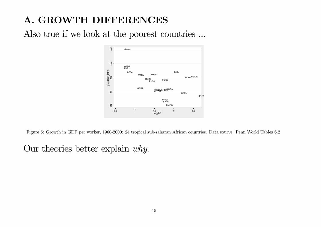
A. GROWTH DIFFERENCESAlso true if we look at the poorest countries ...
BENBFA
BDI
CMR
TCD
COG
CIV
ETH
GHA
GIN
KEN
MDG
MWI
MLIMOZ
NER
NGARWA
SEN
TZA
TGO
UGA
ZMB
ZWE
-.01
0.0
1.0
2.0
3gr
owth
60_2
000
6.5 7 7.5 8 8.5logy60
Figure 5: Growth in GDP per worker, 1960-2000: 24 tropical sub-saharan African countries. Data sourve: Penn World Tables 6.2
Our theories better explain why.
15
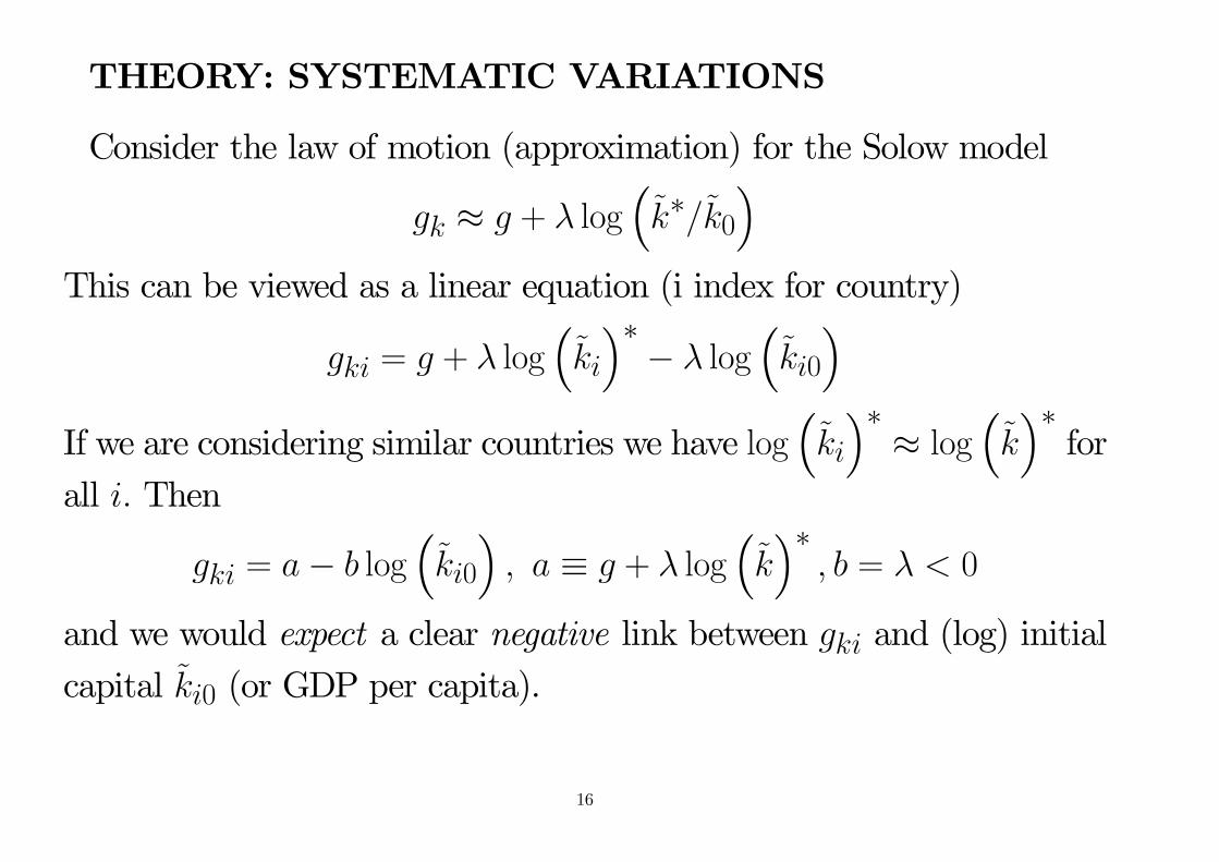
THEORY: SYSTEMATIC VARIATIONS
Consider the law of motion (approximation) for the Solow model
gk ≈ g + λ log³k∗/k0
´This can be viewed as a linear equation (i index for country)
gki = g + λ log³ki
´∗− λ log
³ki0
´If we are considering similar countries we have log
³ki
´∗≈ log
³k´∗for
all i. Then
gki = a− b log³ki0
´, a ≡ g + λ log
³k´∗
, b = λ < 0
and we would expect a clear negative link between gki and (log) initial
capital ki0 (or GDP per capita).
16
In samples where countries are very different, log³ki
´∗6= log
³k´∗for
all i, the same negative association should not (necessarily) arise, unless
we take the differences in log³ki
´∗into account (i.e., s, n and so on).
To fully control for log³ki
´∗the basic Solow model suggests sK and
n. The augmented Solow model would suggest we also need sH. The
Solow model with land would suggest X/L0 should enter as well, and
semi-endogenous growth theory would suggest L0 should enter.
TheAKendogenous growthmodel is NOTconsistent with this evidence.
However an “asymptotic version" can be.
17

THEORY: GROWTH DIFFERENCES
Neoclassical growth theory (Ch. 3,4,5,6, (7..see below)) offerstransitional dynamics. Basically we have
gy ≈ g + λ log (y∗/y0)
growth differences in g are not attractive; hence the “story” is that
countries differ in terms of their distance to steady state
log (y∗/y0)
This is ameaningful story, as themodel suggests λ is fairly low, implying
lengthy transitions. Takes at least 17 years (under plausible parameter
values to reach steady state)
18

THEORY: GROWTH DIFFERENCES
The drawback of this “story” is that every country with less than g
percent growth (say, 2%) per year, are converging from above
Given the growth record, this turns out to be systematically the poorest
countries
Figure 6: Source: Cho and Graham, 1996. Note; The bold faced line is a 45 degree line.
19

THEORY: GROWTH DIFFERENCESThe one exception is the neoclassical growth model with natural re-
sources (Ch 7)!
Here the long-run growth rate is not the same: countries with faster
population growth will growmore slowly in transition and in the steady
state (cf Above)
An alternative account is endogenous growth theory. Here the long-run
growth rate is endogenous (so we can do without “g”). Differences ins (e.g.) will generate difference in growth. Policy can affect s (cf. Ch.
16 on consumption: higher taxes can lower s, for instance). Has its
drawbacks (cf time series evidence)
Semi-endogenous growth: transitional dynamics. Steady state growth∝n. Little evidence that n ↑⇒ gy ↑
20

B. INCOME DIFFERENCES
0,17 0,28 0,390,62
1,00
4,31
5,88
1,38
1,71
2,48
0,00
1,00
2,00
3,00
4,00
5,00
6,00
7,00
10 20 30 40 50 60 70 80 90 100
Percentile
With
in g
roup
med
an G
DP p
er w
orke
r/ G
loba
l med
ian
GD
P pe
r w
orke
r
Figure 7: The numbers refer to the year 2000 and are PPP corrected. Source: World Development Indicators CD-rom 2004.
Moving frommedian in the top group to median of lowest group: Dif-
ference on a scale of 1:35. Our theories should motivate such differences
quantitatively.
21

B. THEORY
The basic Solow model has problems accounting for such vast differ-
ences. Two identical countries, except for s
y∗1y∗2=
µs1s2
¶ α1−α
as s1s2 is at most 1:4,α1−α = 1/2 if α = 1/3. This result is not changed if
we look at the open economy (again, focusing on income differences).
However, adding human capital improves the explanatory power of
physical capital investments:
y∗1y∗2=
µs1s2
¶ α1−α−β
sinceα ≈ β ≈ 1/3, α1−α−β ≈ 1.Reason: Capital-Skill complementarity.
In addition: Human capital levels differ.22

B. THEORY
Drawback: Probably overestimating the importance of human capital
(i.e, putting β = 1/3)
Alternative: Include technology diffusion, so that levels ofA differ. Evidence suggests levels of A differ across countries. Likely
reason: differences in technological sophistication (... as well as other
things: efficiency etc)
A reasonable diffusion model will also generate growth differences in
technology, in transition. That is, a structure like
Awt+1 = (1 + g)Aw
t
Tt+1 − Tt = ω · (Awt − Tt) , ω < 1.
.23

C. CONVERGENCE AND INEQUALITY
0,50
0,60
0,70
0,80
0,90
1,00
1,10
1,20
1,30
1960
1962
1964
1966
1968
1970
1972
1974
1976
1978
1980
1982
1984
1986
1988
1990
1992
1994
1996
1998
Stde
v(lo
ig G
DP
per
wor
ker)
Figure 8: Evolution of Standard deviation of log GDP per worker, 1960-1998. Data: Penn World Tables 6.1.
You tend to find increasing inequality.
24
C. THEORYNeoclassical growth theories (Ch. 3-7) predict conditional convergence.
Hence, neoclassical growth theory does not suggest income differences
across countries will be equalized, unless countries converge in structure
(s,n etc)
Even if countries are similar (but hit by shocks) inequality (appropri-
ately measured) may not decline. The fact that there is a negative link
between growth and initial levels9 Declining inequality (cf. “Galton’s
fallacy)
Another viable hypothesis: Club Convergence. E.g. the subsistence
story, or, endogenous fertility (exercises)
In endogenous growth theory countries with similar characteristics will
converge in growth rates, but not in levels.
25