Output Units of Motor Behavior: An Experimental and ...
20
Output Units of Motor Behavior: An Experimental and Modeling Study E. P. Loeb Gore 2000, Nashville, TN, USA S. F. Giszter Medical College of Pennsylvania and Hahnemann University P. Saltiel and E. Bizzi Massachusetts Institute of Technology F. A. Mussa-Ivaldi Northwestern University Medical School Abstract & Cognitive approaches to motor control typically concern sequences of discrete actions without taking into account the stunning complexity of the geometry and dynamics of the muscles. This begs the question: Does the brain convert the intricate, continuous-time dynamics of the muscles into simpler discrete units of actions, and if so, how? One way for the brain to form discrete units of behavior from muscles is through the synergistic co-activation of muscles. While this possibility has long been known, the composition of potential muscle synergies has remained elusive. In this paper, we have focused on a method that allowed us to examine and compare the limb stabilization properties of all possible muscle combinations. We found that a small set (as few as 23 out of 65,536) of all possible combinations of 16 limb muscles are robust with respect to activation noise: these muscle combina- tions could stabilize the limb at predictable, restricted portions of the workspace in spite of broad variations in the force output of their component muscles. The locations at which the robust synergies stabilize the limb are not uniformly distrib- uted throughout the leg’s workspace, but rather, they cluster at four workspace areas. The simulated robust synergies are similar to the actual synergies we have previously found to be generated by activation of the spinal cord. Thus, we have developed a new analytical method that enabled us to select a few muscle synergies with interesting properties out of the set of possible muscle combinations. Beyond this, the identifica- tion of robustness as a common property of the synergies in simple motor behaviors will open the way to the study of dynamic stability, which is an important and distinct property of the vertebrate motor-control system. & INTRODUCTION There is no doubt that co-activation of muscles is routi- nely observed during the execution of movements, but it is not yet clear how particular combinations of muscles are selected by the central nervous system (CNS) for use in these movements. No natural movement is executed by just one muscle, and common movements involve many muscles. Some muscles produce torques and displacements about joints, while others apparently act to maintain postures and oppose the reaction torques produced by limb displacement. The concept of a ‘‘mus- cle synergy’’ is used to express the notion that there is a functional underlying purpose to the groupings of mus- cles used to execute movements. The use and re-use of muscle groups characterize every movement. The ques- tion is, how is a given muscle group specified by the CNS? In the past, investigators have put forward two radi- cally different views. According to one view, each muscle involved in a task is independently specified by the CNS (Soechting & Lacquaniti, 1989). In this view, apparent muscle synergies are an artifact of the cross-subject commonality of the physics of movements. Alternatively, there are fixed synergies, which are obligatory linkages between muscles. In this later view, the CNS generates movements by recruiting and combining the fixed sy- nergies in a flexible way (MacPherson, 1991). Some of the early ideas about synergies were pro- posed by Sherrington (Sherington, 1961), who con- ceived the muscle synergies as resulting from the activation of specific reflex pathways. Bernstein (1971) also proposed the concept of synergies. He regarded synergies as a way for the CNS to deal with the many © 2000 Massachusetts Institute of Technology Journal of Cognitive Neuroscience 12:1, pp. 78–97
Transcript of Output Units of Motor Behavior: An Experimental and ...

Output Units of Motor Behavior AnExperimental and Modeling Study
E P LoebGore 2000 Nashville TN USA
S F GiszterMedical College of Pennsylvania and Hahnemann University
P Saltiel and E BizziMassachusetts Institute of Technology
F A Mussa-IvaldiNorthwestern University Medical School
Abstract
amp Cognitive approaches to motor control typically concernsequences of discrete actions without taking into account thestunning complexity of the geometry and dynamics of themuscles This begs the question Does the brain convert theintricate continuous-time dynamics of the muscles intosimpler discrete units of actions and if so how One way forthe brain to form discrete units of behavior from muscles isthrough the synergistic co-activation of muscles While thispossibility has long been known the composition of potentialmuscle synergies has remained elusive In this paper we havefocused on a method that allowed us to examine and comparethe limb stabilization properties of all possible musclecombinations We found that a small set (as few as 23 out of65536) of all possible combinations of 16 limb muscles arerobust with respect to activation noise these muscle combina-
tions could stabilize the limb at predictable restricted portionsof the workspace in spite of broad variations in the forceoutput of their component muscles The locations at which therobust synergies stabilize the limb are not uniformly distrib-uted throughout the legrsquos workspace but rather they clusterat four workspace areas The simulated robust synergies aresimilar to the actual synergies we have previously found to begenerated by activation of the spinal cord Thus we havedeveloped a new analytical method that enabled us to select afew muscle synergies with interesting properties out of the setof possible muscle combinations Beyond this the identifica-tion of robustness as a common property of the synergies insimple motor behaviors will open the way to the study ofdynamic stability which is an important and distinct propertyof the vertebrate motor-control system amp
INTRODUCTION
There is no doubt that co-activation of muscles is routi-nely observed during the execution of movements but itis not yet clear how particular combinations of musclesare selected by the central nervous system (CNS) for usein these movements No natural movement is executedby just one muscle and common movements involvemany muscles Some muscles produce torques anddisplacements about joints while others apparently actto maintain postures and oppose the reaction torquesproduced by limb displacement The concept of a lsquolsquomus-cle synergyrsquorsquo is used to express the notion that there is afunctional underlying purpose to the groupings of mus-cles used to execute movements The use and re-use ofmuscle groups characterize every movement The ques-tion is how is a given muscle group specified by the CNS
In the past investigators have put forward two radi-cally different views According to one view each muscleinvolved in a task is independently specified by the CNS(Soechting amp Lacquaniti 1989) In this view apparentmuscle synergies are an artifact of the cross-subjectcommonality of the physics of movements Alternativelythere are fixed synergies which are obligatory linkagesbetween muscles In this later view the CNS generatesmovements by recruiting and combining the fixed sy-nergies in a flexible way (MacPherson 1991)
Some of the early ideas about synergies were pro-posed by Sherrington (Sherington 1961) who con-ceived the muscle synergies as resulting from theactivation of specific reflex pathways Bernstein (1971)also proposed the concept of synergies He regardedsynergies as a way for the CNS to deal with the many
copy 2000 Massachusetts Institute of Technology Journal of Cognitive Neuroscience 121 pp 78ndash97
degrees of freedom that are involved in the generationof movement1 A synergy in Bernsteinrsquos terms is ameans or the means to reduce the number of mechan-ical variables involved in the execution of even thesimplest movement
In this work we have investigated muscle synergiesfrom a new perspective we have taken the point of viewthat a collection of co-activated muscles is equivalent toa forcing function acting on the limb dynamics Tounderstand the concept of a forcing function suspenda series of weights from a rubber band When the weightchanges the rubber band will stretch and bounce but itwill eventually settle down at a new length determinedby the total magnitude of the weight it is bearing Theweight is a forcing function The rubber band is adynamic system The rubber band has a temporal re-sponse to the onset of the forcing functionmdashitbouncesmdashbut after that it settles into its new steadystate which is dictated by the forcing function In asimilar manner the limb should ultimately settle into asteady state dictated by the total forces exerted bygravity friction objects in the environment and thesum total of the forces exerted by the individual mus-cles Thus we have approached the problem of under-standing muscle co-activations by examining musclesand combinations of muscles as forcing functions
The key instrument that has made this explorationpossible is the representation of a musclersquos action as aforce field Our force fields map limb postures to theforce acting on the ankle at that limb posture A forcefield is a forcing function All else being equal we expectthe ankle (and the limb with it) to accelerate in thedirection of any force acting on it If the force fieldcontains a Convergent Equilibrium Point (CEP) wherethe force is zero and towards which the other forcespoint then we would expect the limb to move to theposition of the CEP and stay there
In order to predict the limb stabilization properties ofcombinations of muscles we have measured the forcefields produced by individual muscles and then com-bined those force fields The bulk of this study concernsthe validation of the method We first developed andtested several different models of individual musclesWe then performed statistical tests to verify that themodeled muscles made correct predictions of theforces produced by individual muscles and combina-tions of muscles Finally we verified our use of distribu-tions of CEP locations Figure 12 shows that we cancorrectly predict the distributions of CEPs that areobserved during four commonly occurring muscle co-activations
Having verified the predictive accuracy of our forcefield models we proceeded to ask where can eachcombination of muscles stabilize the limb and how likelyis it to do so We approached this question by examiningrandom activations of the muscles in each possiblemuscle combination In this way we could estimate
the probability of producing a stabile posture (a CEP)and the locus of limb postures at which those CEPsoccurred Our analysis has led to the surprising resultthat in the large space of simulated muscle combinationsthere exists a well-defined subset of synergies which willstabilize the limb despite activation noise muscle fati-gue and other uncertaintiesmdashand these synergies sta-bilize the limb at predictable restricted locations in theworkspace So according to our model these robustmuscle synergies can be depended on to get the limb tothe right place We observed that the robust musclesynergies bring the limb to four discrete locations in theworkspace which are near to the four discrete CEPlocations we have found to be evoked by microstimula-tion of the interneuronal areas of the frogrsquos spinal cord(Bizzi Mussa-Ivaldi amp Giszter 1991 Giszter Mussa-Ivaldi amp Bizzi 1993 Loeb Giszter Borghesani amp Bizzi1993 Saltiel Tresch amp Bizzi 1998) We conclude thatthe frog at least may make use of noise-resistant musclesynergies to correct for the vagaries of the force outputof individual muscles
RESULTS
Model force fields of 16 hindlimb muscles are shown inFigures 1 2 3 4 5 and 6 We have grouped the musclesinto six types according to the similarities that we see inthese models2 Figure 1 shows the Hip ExtensorKneeFlexor muscle type These muscles (AD RI and ST)extend the hip and flex the knee Figure 2 shows theBody Flexor muscle type These muscles (BI and SA)predominantly flex the knee Figure 3 shows the RostralFlexor muscle type These muscles (IP and PT) predo-minantly flex the hip Figure 4 shows the Half Flexormuscle type These muscles (ADl GA and RA) flex thehip andor the knee and produce no force when the hipis flexed Figure 5 shows the Hip Extensor muscle typeThese muscles (QF and SM) predominantly extend thehip Figure 6 shows three muscles acting as lateralextensors These muscles (PE VE and VI) extend theknee and may flex the hip as well3
Inspection of Figures 1 2 3 4 5 and 6 indicates thatno muscle has an equilibrium point in the limbrsquos work-space Neither the individual musclesrsquo recorded forcefields nor the models appeared to be stable in theworkspace Some muscles display near-zero forces inthe part of the workspace towards which their forcespoint In these muscles the general flow of the musclersquosforce fields appears to pull the ankle to a part of theworkspace where the magnitude of the musclersquos forcebecomes negligible All of the half flexors (ADl GA andRA Figure 4) have this property as do RI and RIm(Figure 1) SA (Figure 2) and VI (Figure 6) Suchmuscles could be used by the spinal circuitry to selec-tively modulate forces in some parts of the workspacewithout affecting the forces generated in other parts ofthe workspace
Loeb et al 79
For each of the 16 leg muscles of six frogs wecomputed the correlation values between the recordedmuscle force fields and the corresponding force fieldmodel for that muscle The histogram of correlationvalues for 96 recorded muscles has a median correlationvalue of 871 (Figure 7) This histogram indicates thatthe model force fields have captured the main featuresof the experimentally derived force fields
Prediction of End-Point Force from Models andEMGs
To validate the linear combination of muscle models weused measured electromyographic (EMG) signals andtheir corresponding model muscle force fields to predictthe total force observed at the limbrsquos end-point TheEMG signals and the end-point forces were recordedduring spinal microstimulation (Bizzi et al 1991 Giszter
et al 1993) We used the EMG signals to scale themuscle model forces and summed the scaled models togenerate predictions of the forces that should be ob-served at the ankle during the time that the EMGs wererecorded (see Methods section) Since we were in factmeasuring the forces at the ankle at the time the EMGswere recorded we were able to compare the predictedankle forces to the observed ankle forces Figure 8shows that there is good qualitative agreement betweenthe observed and predicted forces
In Figure 9 we quantify the degree of correlationbetween actual and predicted end-point forces Wefound a high correlation (R2=864 F(33 160)=369plt001) between predicted and actual endpoint forceorientations for 244 spinal stimulation trials in threeanimals There are 33 free parameters in the F-statisticbecause 11 EMG gains were computed for each of thethree animals in the dataset Ninety-five percent of the
Figure 1 The hip extensorknee flexor muscles Adductor Magnus (AD) Rectus Internus (RI) Semitendinosus (ST) and Rectus Internus Minor(RIm) all function as hip extensors and knee flexors Note muscles RI and RIm have zero-force regions toward which their forces point The meanforce field correlations of the models with their data force fields are 076 (AD 7 frogs) 085 (RI 6 frogs) 087 (ST 5 frogs) and 091 (RIm 3 frogs)This figure and Figures 2 3 4 5 and 6 are constructed as per Figure 1B using the modeled data at each limb position for which we collected datafrom any frog used in the model
80 Journal of Cognitive Neuroscience Volume 12 Number 1
trials in the figure have a prediction error strictly lessthan 458 Thus we are able to account for a large portion(86) of the variance in peak force orientation using ourmuscle models and observed EMG signals
Simulated Synergies Combining Musclesrsquo ForceField Models
The main result of this work is a new method foranalyzing muscle synergies We simulated the forcefieldsresulting from all possible combinations of 16 modelmuscles Our simulation resulted in an estimated dis-
tribution of CEPs for the 216=65536 combinations ofmusclersquos force fields that are possible with 16 musclesAs activation coefficients for the muscle models we usedrandom numbers [0 to 100] instead of using the EMGsused in the previous section The algorithm for themuscle combination simulation is as follows (see Meth-ods section)
1 Select a muscle combination C2 Estimate CEP distribution of C (Figure 10)3 Weight each muscle in C by a random value4 Sum the weighted muscle model force fields
Figure 2 The body flexor muscles Biceps (BI) and Sartorius (SA) function predominantly as knee flexors The flow of forces are reminiscent of theflexion-to-body behavior of spinalized frogs The mean force field correlations of the models with their data force fields are 081 (BI 8 frogs) and085 (SA 9 frogs)
Figure 3 The rostral flexor muscles Ilio-Psoas (IP) and Pectineus (PT) function as hip flexors The flow of forces are reminiscent of thepreparatory rostral flexion phase of the back wiping behavior of spinalized frogs The mean force field correlations of the models with their dataforce fields are 078 (IP 5 frogs) and 090 (PT 3 frogs)
Loeb et al 81
5 Does resulting force field converge Where6 Store the answers and return to step 27 Compute and store the (x y) location of the
joints space centroid of the CEP locations determinedin steps 2 through 6
The loop in step 2 was typically performed 50ndash500times for each muscle combination Step 2 results in anestimate of the probability of convergence and a dis-tribution of the convergence locations for the givenmuscle combination C (See Figure 10D)
In Figure 11 we plot the stored CEP centroids pro-duced by the muscle combination simulation for thou-sands of different muscle combinations Although theCEP locations for a single muscle combination are oftenscattered throughout the workspace we have summar-ized each combinationrsquos CEP distribution with a singledot (at the centroid of its CEP distribution) for thepurpose of this figure
In Figure 11A we show the centroids of reliablemuscle combinations These are muscle combinationsthat produced a convergent force field with 95 or moreof the random activation patterns we tried There are14256 reliable combinations out of 65536 possiblecombinations So there are 14256 dots in Figure 11AEach dot is the centroid of one muscle combinationrsquosdistribution of convergent equilibria
In Figure 11B we show the centroids of the localizedmuscle combinations These are the combinations thatproduced CEPs that always fell within some 5000 squaredegree area in the workspace (approximately 708 max-imum excursion in hip angle and knee angle) Thecutoff 5000 square degrees is one standard deviationbelow the mean localization value in Figure 15B
In Figure 11C we have plotted the 909 (out of 65536)centroid locations of combinations which we havenamed robust These combinations are lsquolsquoreliablersquorsquo andlsquolsquolocalizedrsquorsquo They produce CEPs for at least 95 of the
Figure 4 The half-flexor muscles Rectus Anticus (RA) Gastrocnemius (GA) and Adductor Longus (ADl) all function as hip or knee flexors All 3muscles have vanishing moment (0 forces) when the hip is flexed The mean force field correlations of the models with their data force fields are090 (RA 6 frogs) 084 (GA 8 frogs) and 072 (ADl 4 frogs)
82 Journal of Cognitive Neuroscience Volume 12 Number 1
Figure 5 The hip extensor muscles Semimembranosus (SM) and Quadratus Femoris (QF) function as hip extensors The mean force fieldcorrelations of the models with their data force fields are 089 (SM 8 frogs) and 083 (QF 4 frogs)
Figure 6 The lateral extension muscles Peroneus (PE) Vastus Internus (VI) and Vastus Externus (VE) all function as knee extensors with musclesVE and VI also acting as hip flexors The mean force field correlations of the models with their data force fields are 078 (PE 5 frogs) 062 (VI 8frogs) and 090 (VE 6 frogs)
Loeb et al 83
random activation patterns we tried and the resultingCEPs were entirely contained within some 5000 squaredegree portion of the workspace
The robust combinations displayed in Figure 11C arenot uniformly distributed but cluster in three or possi-bly four groups It is of interest that there is a degree ofcorrespondence between CEPs of these robust combi-nations and the CEPs of force fields evoked by micro-stimulation of the spinal cord (Bizzi et al 1991 Giszteret al 1993) The degree of correspondence is evenmore marked when more restrictive criteria of robust-ness are applied In Figure 11D the criterion of relia-bility was increased to 98 and the localization cutoffwas decreased to 1600 square degrees (sup1408 per joint)
Comparison of Simulated and Experimental ForceFields
The rough correspondence between the CEPs of therobust combinations and the CEPs of spinally-evokedforce fields raises the question whether the muscles thatimplement the spinally-evoked fields belong to the classof robust synergies To address this question we appliedthe simulation procedure to the groups of muscles thatwere experimentally found to be active during spinalmicrostimulation
In Figure 12 we see the degree of overlap betweenactual and simulated CEP distributions for the empiricalmuscle synergies For example in Figure 12 (upperright) the simulated distribution for the muscle combi-
nation (AD GA PE and RI) is represented by one reddot for each simulated CEP These red dots completelycover the observed distribution of CEP locations evokedby microstimulation trials producing Caudal Extension(area E see Saltiel et al 1998) force fields We haveobserved that Caudal Extension force fields are asso-ciated with the muscle combination (AD GA PE andRI) and random activation of these five muscle modelsproduced the scatter of CEPs shown in red in Figure 12(upper right) The mean of the random computed CEPssubstantially overlaps the observed CEP distribution sothe predictive accuracy of the muscle models is againconfirmed However the distribution of the computedCEPs is too broad for this combination to be robust bythe definition of Figure 11C
Similarly in Figure 12 upper left lower left and lowerright the computed CEP distribution overlaps the ob-served CEP distribution for the set of muscles testedThus we were able to confirm (qualitatively) the pre-dictive accuracy of our estimated CEP distributions
A detailed inspection of Figure 12 reveals that thesimulation of experimentally-evoked synergies leads to ahigh density of their equilibria in certain regions of theworkspace For example in Figure 12 (upper right) wefound that the broadness of the scatter of equilibriumpoints is mostly attributable to the muscle SA When SAis weakly activated the scatter of CEPs is small becausethe other muscles (that is all muscles in the combina-tion except for SA) are a robust muscle synergy Con-versely when the activation of muscle SA is large relativeto the other muscles in the combination the CEPs aremore broadly scattered This logic applies to all of thepanels in Figure 12 They all show dominant clusteringat the locus of a robust synergy with weak additionalscatter due to the other muscles In contrast to thesimulations the experimental CEP distributions are lessbroadly scattered and two are restricted to the regionsof dense clustering (Figure 12 upper left and Figure 12upper right) The range of muscle activations induced bythe stimulation of spinal interneurons may be particu-larly constrained for those muscles that tend to induce alarge excursion of the CEP
DISCUSSION
This paper has four key points
1 We present a novel method for exploring theaction of muscle synergies We characterize musclesynergies as probability distributions of (in particular)CEP locations in the limbrsquos workspace
2 We have used CEP distributions as a tool toexamine a few naturally occurring synergies In parti-cular we asked if the spinal cord uses muscle synergiesthat are robust to activation noise
3 We have collected new data on the action inthe x y plane of 16 hindlimb muscles of the frog
Figure 7 Correlation between recorded muscle force fields andmuscle models Histogram showing force field correlation value on thex axis and the number of force fields on the y axis This histogramprovides an overview of the mean correlation values given in thelegends of Figures 1 2 3 4 5 and 6 For each frog and each muscle wecomputed the correlation between the measured force field for thatmuscle and the model of that muscle constructed from themeasurement of all the frogs The figure shows that 35 of the 96recorded muscle force fields correlated with their model force fields ata level of 90 or greater
84 Journal of Cognitive Neuroscience Volume 12 Number 1
None of the muscles could individually stabilize thelimb
4 We developed a new method for modelling theforce produced by leg muscles
The Distributions Associated with MuscleSynergies
We used combinations of muscle models to associateeach possible muscle synergy with a probability distribu-tion of CEP locations in the workspace By convertingsynergies to distributions we were able to examine theentire set of muscle synergies quantitatively because wewere able to compare the distributions For example
once we determined the likelihood of convergence foreach muscle combination we were able to select thesynergies that had a high likelihood of convergencerelative to all the other synergies This general methodcan be extended to many other features of interest Herewe have focused on distributions of equilibrium pointsbut it is also possible to examine distributions of forcesdynamic variables and so forth
Does the Spinal Cord Use Robust Synergies
Electrical or chemical microstimulation of the pre-motorneuronal circuitry of the spinal cord of thefrog produces precisely balanced contractions in
Figure 8 Forces recorded atthe ankle produced by spinalstimulation are compared withmodel forces (A) The tracesalong the top row are (from leftto right) the observed (x y)forces the predicted (x y)forces and the filtered EMGsignal from the following mus-cles RA RI AD SM ST VI BISA VE TA and GA (B) Threemore observed and predictedforce traces from the sameanimal
Loeb et al 85
groups of leg muscles These synergistic contractionsgenerate forces that direct the limbrsquos end-pointtoward an equilibrium point in the workspace ofthe leg
To record the spatial variations of forces that aregenerated by the leg muscles Bizzi et al (1991)Giszter et al (1993) and Saltiel et al (1998) stimulatedsites in the spinal cord and recorded the direction andamplitude of the elicited isometric force at the ankleThey found that the elicited force vectors varied asthey placed the limb at different locations The collec-tion of the measured forces corresponded to a forcefield
Different groups of leg muscles were activated as thestimulating electrodes (or pipettes) were moved todifferent loci in the lumbar spinal cord in the rostrocau-dal and mediolateral direction After mapping most ofthe premotor area of the lumbar cord Bizzi et al (1991)Giszter et al (1993) and Saltiel et al (1998) reached theconclusion that there were at least four areas fromwhich distinct types of convergent force fields couldbe elicited
In this paper we performed an exhaustive simula-tion of the limb stabilizing abilities of all combinationsof 16 muscles Within these 65536 possible musclesynergies we found a small subset that should ac-cording to our model be robust in the face of thevarious sources of noise with which the motor controlsystem must contend In particular these robust sy-nergies are lsquolsquoreliablersquorsquo and lsquolsquolocalizedrsquorsquo They are reli-
able because they produce convergent force fields foralmost all of the random patterns of activation wetried Thus we expect these synergies to stabilize thelimb even if (for example) one of the muscles isfatigued The robust synergies are localized becausetheir CEP locations fall within a relatively small area inthe workspace Thus we expect these synergies tostabilize the limb at a predictable location even if (forexample) changes in ambient temperature cause thesurface muscles to be less effective than the deepermuscles Reliability and localization combined makethe robust synergies apparently useful as buildingblocks of limb stability
The composition and the behavior of the robustsynergies is correlated to the composition and beha-vior of the synergies that are evoked by electrical andchemical stimulation of the spinal cord Composition-ally the evoked synergies always contain at least onerobust synergy Behaviorally the evoked synergiesproduce CEP locations in the same portions of thelegrsquos workspace as the robust synergies It remains tobe investigated whether the robust synergies are usedas building blocks as these findings suggest Thepreservation of stability in the face of variable effectsof control signals (due to muscle fatigue muscletemperature limb velocity muscle stiffness and im-mediate activation history) presumably plays an im-portant and fundamental role in motor controlsystems
Models of the Legrsquos Muscles
We described a statistical model of the frogrsquos muscleswhich accurately predicts the orientation of the forcevectors generated by the activation of individual legmuscles The models utilized in this study were con-structed by least-squared-error parameter estimationtechniques This approach has made it possible to avoiddifficult measurement problems Previous muscle mod-els were based on actual measurements of musclelength and musclersquos moment arm derived from cadavers(Loeb He amp Levine 1989 Wickland Baker amp Peterson1991) These measurements rely heavily on mathema-tical simplifications of the intricacies of muscle geometryin order to compute muscle length as a function of thejoint angles for each modeled muscle (Buchanan Alm-dale Lewis amp Rymer 1986 Wickland et al 1991Winters amp Stark 1988 Zajac and Winters 1990) How-ever it is unclear how well muscle geometric para-meters generalize across subjects and these invasivemeasurements are not practical in all settings In thisstudy we have instead constructed muscle length func-tions from measurements of endpoint forces induced bymuscle stimulation at different joint angles (see Meth-ods Section)
We utilized our muscle models to predict the forcesrecorded at the ankle following spinal microstimula-
Figure 9 Summary statistics for force predictions from a largedatabase We used 244 spinal stimulation trials from three animals totest the accuracy of force predictions from EMG signals Fifteenpercent of the trials from each animal were used to create 11 EMG gainfactors per animal (one gain for each recorded muscle in each animal)These trials were then removed from the dataset Thus there were noparameters determined by the data in this figure The remaining 200trials are shown here The trials are labeled lsquolsquo4rsquorsquo lsquolsquo5rsquorsquo and lsquolsquo6rsquorsquo after theiranimal labels The inset illustrates the method used to comparePredicted and Observed force traces (see Methods)
86 Journal of Cognitive Neuroscience Volume 12 Number 1
Figure 10 Monte Carlo simulation analysis of a single muscle combination The force fields produced by random activations of muscles arecomputed so as to summarize each muscle combinationrsquos distribution of CEPs (A) The binary vector encoding BI+RI+ST+SA (B) Threerandom activation patterns conforming to the BI+RI+ST+SA muscle combination All muscle activation values are zero except for the fourmuscles in the combination The non-zero activation values are random numbers chosen from a uniform distribution over [0 100] (C) Thethree force fields resulting from the three activation patterns in (B) The force fields are computed in the manner of Figure 7 using therandom activation values instead of gains and EMGs For example the forces in the first (left-most) force field are 127 times the forces of theBI muscle model plus 246 times the forces of the RI muscle model and so on The three illustrated force fields all converged their equilibriaare indicated by the large dots (D) Distribution of the CEP locations for BI+RI+ST+SA We sampled 2000 activation patterns forBI+RI+ST+SA and 66 (1322) of those sampled activation patterns led to convergent force fields A stick-figure leg is shown with its ankle atthe centroid of the distribution of the CEP locations The ellipse surrounding the centroid has major and minor axes given by twice the (jointspace) standard deviation The whale-like shape surrounding the stick-figure leg is the boundary of the workspace (hipgtndash 1108 and lt808kneegt108 and lt1708)
Loeb et al 87
tion Previous investigations (Mussa-Ivaldi Giszter ampBizzi 1994) showed that the simultaneous activation oftwo muscles lead to a force field which is the vectorsum of each musclersquos force field In this investigationwe needed to consider the concurrent mechanicaleffect of several muscles In order to asses the validityof the vector summation with such muscle popula-tions we have used the EMG signal measured in eachmuscle We simulated the net spinal field as the sumof muscle fields each one scaled according to theamplitude of the EMG measured in the actual spinalstimulation Our results indicate that there is indeedan excellent agreement between measured and pre-dicted forces This finding demonstrates that it ispossible to model the activation of multiple muscles
as a weighted combination of the empirically derivedmuscle models
Conclusion
We have developed a method that allowed us to identifymuscle synergies with special properties out of a largeset of possible muscle combinations This methodwhich is based on the modelling of the force generatedby individual muscles will allow us to examine therobustness of muscle combinations not only duringposture (as we did here) but also in a variety of othercircumstances such as reflex activation and centrallygenerated movements Finding properties of robustnessof synergies in these motor behaviors will open the way
Figure 11 Reliable localized and robust CEP distributions The centroids of CEP distributions are shown (A) The 14256 centroid locations ofthe reliable muscle combinations These centroids lie away from the body because the extensor muscles are stronger (B) The 9538 centroidlocations of the localized muscle combinations (C) The 909 centroid locations of the robust muscle combinations Points are plotted here only ifthey are plotted in both (A) and (B) (D) The 23 combinations fitting a (reliability localization) cutoff of (98 1600 square degrees) Each of these23 robust distribution is drawn here with an lsquolsquoOrsquorsquo at its centroid within an ellipse covering plusmn1 SD in CEP location The CEP distribution ellipsesobserved during spinal microstimulation are also shown for comparison These ellipses are labelled R for Rostral Flexion B for Body Flexion W forWipe E for Caudal Extension and L for Lateral Extension
88 Journal of Cognitive Neuroscience Volume 12 Number 1
Figure 12 (Upper Left) The rostral flexion combination There are seven muscles in this combination BI GA IP PE RA SA and ST Wehave observed Rostral Flexion hindlimb forces in conjunction with this muscle combination The distribution of red computed CEPs(summarized in light blue) overlaps the green distribution of observed Rostral Flexion equilibrium points The red distribution has reliability29 and localization 21837 square degrees The sub-combination BI+GA+PE+RA+SA is robust (Upper Right) The caudal extensioncombination There are five muscles in this combination AD GA PE RI and SA We have observed Caudal Extension hindlimb forces inconjunction with this muscle combination The distribution of red computed CEPs covers the green distribution of observed Caudal ExtensionCEPs The red distribution has reliability 993 and localization 25440 square degrees The sub-combination AD+PE+RI is robust (Lower Left)The lateral extension combination There are 10 muscles in this combination GA IP PE RA SA and VI are strong AD RI SM and VE areweak We have observed Lateral Extension hindlimb forces in conjunction with this muscle combination The distribution of red computedCEPs overlaps the green distribution of observed Lateral Extension equilibrium points The red distribution has reliability 994 andlocalization 15594 square degrees This large combination of muscles has several robust sub-combinations (Lower Right) The hindlimb wipecombination There are seven primary muscles in this combination AD BI IP RA RI SA and ST We have observed both Body Flexion andHindlimb Wipe forces in conjunction with this muscle combination The distribution of red computed CEPs overlaps the green distributions ofobserved Body Flexion and Hindlimb Wipe equilibrium points The red distribution has reliability 82 and localization 15904 square degreesThe sub-combination AD+RA+RI+SA+ST is robust
Loeb et al 89
to the study of dynamic stability which is an importantand distinct property of the vertebrate motor controlsystem
METHODS
Surgery and Data Collection
Twenty-four healthy adult bullfrogs (Rana Catesbiana)were anesthetized with 05ndash15 cm3 tricaine and spina-lized anterior to the first vertebra The skin of the righthindlimb was removed and the muscles were coatedwith Vaseline to keep them moist The superficial fasciawere cut to allow access to deep muscles and nervesAll large nerves were cut and removed to sever thereflex arcs and to prevent the stimulus applied to onemuscle from spreading along the nerves to othermuscles
A pair of lsquolsquofishhook electrodesrsquorsquo (stainless steel wirethreaded through a syringe needle with exposed wire atthe tip bent back to form a hook (Crago Peckham ampThrope 1980)) were placed in each muscle under adissecting microscope Stimulus voltage was set at the
start of each experiment to evoke a maximal visiblemuscle contraction without causing contractions in anyother muscles The surgical isolation of the musclesmade it possible to verify isolated responses by visualinspection of the muscles Another criterion for detect-ing the spread of activity to other muscles was thesudden change of force orientation at the endpoint ofthe limb This change was readily detected when thestimulus voltage exceeded a certain threshold Theother stimulation parameters were fixed at 06 msecpulses width 600 msec train duration and 40 Hz
Recording Force Fields from Individual Muscles
Spinalized frogs were placed on a moistened moldedplastic frame and secured in place by clamps attached tothe pelvis The position of the frogrsquos hip in the apparatusand the length of its right hindlimb segments weremeasured The right ankle was attached to a force sensorimmediately proximal to the frogrsquos ankle The forcesensor was attached to a frame which enabled us tochange the ankle coordinates in the horizontal (x y)
Figure 13 This figure illustrates the processing steps taken to produce a force field from the data recorded during muscle stimulation (A)Illustration of a frog in the standard coordinate frame of our experimental apparatus Our Cartesian coordinate system is defined by a fixed metalstand at position (0 0) on which the sensor is mounted (not shown) The right hindlimb is shown at a hip angle of 268 measured counter-clockwisefrom the horizontal and a knee angle of 838 measured counter-clockwise from full flexion The standard frogrsquos thigh and calf lengths are both 60mm These configuration parameters correspond to an anklesensor position of (62 mm ndash 74 mm) in the workspace The schematic spring attachedto the limb represents the muscle Semimembranosus When the muscle is stimulated the force sensor records the translational (x y) forces (B)Recorded (x y) force traces induced by stimulation of a frogrsquos Semimembranosus muscle are plotted as a sequence of vectors The vector with thegreatest magnitude is highlighted (C) A force field is constructed from the peak force vector at each tested limb position The circled forcecorresponds to the limb position in (A) and the peak force in (B)
90 Journal of Cognitive Neuroscience Volume 12 Number 1
plane The Z coordinate of the ankle was kept unchangedand approximately level with the hip (Figure 13A)
We measured a muscle force field by stimulatingone muscle with the hind limb positioned in each ofmany different locations Thus we followed this sim-ple procedure (Giszter et al 1993) (1) Stimulate onemuscle while measuring force (2) Move the ankle to anew position (3) Repeat from step 1 for the samemuscle
As the muscle contracted and relaxed in response tostimulation the force sensor recorded x- and y-forcesas a function of time (Figure 13B) Forces were digi-tized and recorded in units of 001 N We initiated ourforce measurements 50 to 200 ms prior to stimulusonset We used the first 50 msec of the forcersquos recordto estimate the baseline force levels We computed theactive force traces by subtracting the baseline forcelevel from the total force measured during musclestimulation
The active forces were time-variant but they could beapproximated as time-invariant because the active forcevectors typically rose and fell along a single orientation(Figure 13B) Thus a whole temporal sequence of activeforce vectors was represented as a single vector modu-lated by a scalar signal We used the active force vectorwith the largest magnitude to represent the entire forcetrace4 The peak active force vectors from each testedankle position form a time-invariant force field FFi(x y)(Figure 13C)
To correct for the frogsrsquo different sizes we convertedthe measured forces to joint torques (Lan amp Crago1992) Then we normalized the joint torques acrossanimals by scaling each frogrsquos torque data at a standardposture to the same value of magnitude for all frogs
Finally we converted the normalized torques back toforces using standardized link lengths of 60 mm
Models Representing the Force Field of IndividualMuscles
The rationale for establishing force field models ofindividual muscles rests upon the need to obtain foreach muscle a simple function that can be manipulatedanalytically To this end we developed statistical modelsusing a least-squares procedure based upon the forceswe recorded from individual muscles We considered anumber of different models We tested the ability ofeach model type to generalize to new data using theJackknife technique (Efron and Tibshirani 1982) Weperformed the Jackknife tests on a dataset of force fieldsobserved during the stimulation of muscles in ninefrogs
Table 1 shows the average generalization errors wefound for several muscles and model types The general-ization errors were measured as root mean squaretorque errors and as force field correlations (Giszteret al 1993 Mussa-Ivaldi et al 1994) Small root meansquare errors and large correlation values indicate that amodel should generalize well over new data Table 1shows that the lsquolsquovirtual workrsquorsquo model type (describedbelow) had the smallest errors of the five model typeswe compared
The Virtual Work Model Type
Our virtual work model consists of a parameterizedmuscle length function and a fixed lengthndashtension curveWe derived this model from the invariance of work
Table 1 Jackknife Errors for Five Model Types
Muscle N Frogs Mean Torque Linear Torque Nine Gaussians Gated Experts Virtual Work
SM 9 432 (66) 387 (68) 467 (77) 255 (79) 227 (87)
SA 9 445 (73) 373 (73) 369 (78) 265 (76) 249 (79)
ST 5 222 (72) 285 (83) 241 (87) ndash 156 (83)
AD 7 629 (71) 62 (67) 416 (69) 166 (66) 159 (68)
VI 8 288 (59) 336 (52) 35 (65) ndash 213 (55)
IP 6 285 (44) 327 (51) 278 (58) ndash 271 (57)
VE 6 357 (82) 363 (75) 225 (78) 25 (78) 245 (80)
Root mean squared error and mean force field correlation (in parenthesis) are displayed for seven hindlimb muscles and five model types TheJackknife technique involves fitting model parameters with data from all the frogs except one and then using that fitted model to predict the datafrom the frog that was left out This fit-and-predict operation is repeated once for each frog in the dataset in order to compute an averagegeneralization error The root mean squared error is the square root of the average of the square of the error The force field correlation value offorce field A and force field B is the correlation value for the vectors (x1A x2A xNA y1A y2A yNA) and (x1B x2B xNB y1B y2B yNB)where xiA is the x component of the force at position i of field A Low squared errors and high force field correlations indicate good generalizationFor example the Mean Torque model type would be expected to have a root mean square prediction error of 432 torque units (001 Nrad) on newSemimembranosus data whereas the Virtual Work model would be expected to have an error of 227 N Frogs is the number of animals in thedataset for each muscle The Mean Torque model predicted joint torques as the mean of the observed joint torques The Linear Torque modelpredicted torque as fitted (constant plus one linear term) function of the joint angles The nine Gaussians model (Mussa-Ivaldi 1992) and the GatedExperts model ( Jacobs amp Jordan 1993) are described elsewhere They both have more free parameters than the Virtual Work model
Loeb et al 91
(force times displacement) with respect to coordinatetransformations
muscle work ˆ tension centlength ˆ skeletal workˆ torqueT d q hellip1dagger
where centlength is an infinitesimal change in musclelength d q is an infinitesimal change in the vector of jointangles and torqueT is the transpose of the vector ofjoint torques Muscle tension is the linear force exertedby the muscle5
The coordinate transformation for a muscle is thefunction length( q ) that transforms the joint coordinatesystem of joint angles q into the muscle coordinatesystem of muscle lengths Rearranging Equation 1 wehave an equation for the torque vector produced by asingle muscle
torque ˆ tension curren hellipcentlengthhellip q dagger= d q daggerT hellip2dagger
We used the relation in Equation (2) to convert ourmuscle stimulation data into muscle models Its secondterm (centlength( q ) d q )T is a vector of derivatives Thuswe can compute the right side of the equation from asimple length function provided the muscle tension is
a simple function of muscle length and provided thatwe can compute the two required derivatives of thelength function There are many different lengthfunctions for which this is possible and we usedsinusoids (Lieber amp Boakes 1988 Lieber amp Shoemaker1992) as follows
length(hip angle knee angle)ˆ L0 Dagger Ah curren coshellipfreqh curren hip Dagger phihdagger Dagger Ak
curren coshellipfreqk curren knee Dagger phikdagger
There are seven external parameters in our lengthfunction L0 Ah freqh phih Ak freqk and phik Theparameters with the lsquolsquohrsquorsquo subscript refer to the part ofthe muscle-length function that depends on the hipangle The parameters with the lsquolsquokrsquorsquo subscript refer tothe part of the muscle-length function that depends onthe knee angle Note that the derivatives of this lengthfunction with respect to hip angle and knee angle areboth easy to determine
For the lengthndashtension function we used a sigmoid
tension(hip knee) ˆ scalecurren sigmoid(length(hip knee))
Table 2 Virtual Work Muscle Model Variable Values for 16 Frog Hindlimb Muscles
Muscle L0 Ak Freqk Phik Ah Freqh Phih Scale
AD ndash 036 271 ndash 0894 0826 537 0702 ndash 107 1060
ADI ndash 1330 0353 148 ndash 25 1330 00234 0061 2720
BI 2790 3340 014 214 ndash 160 209 365 347
GA 140 487 ndash 164 262 153 00658 273 454
IP 246 ndash 104 199 ndash 11 104 0634 143 969
PE 239 725 ndash 0888 243 386 0613 255 1050
PT ndash 604 782 ndash 00286 ndash 00912 527 0042 0046 3540
PY 1380 1570 00186 616 2950 00228 32 595
QF ndash 101 0789 ndash 106 318 ndash 0486 0612 418 173e+08
RA ndash 4940 0459 ndash 11 ndash 294 4930 00153 003 469e+06
RI 394 113 ndash 113 0832 403 00371 ndash 291 5570
RIm ndash 149 ndash 156 ndash 00626 322 ndash 764 ndash 0657 ndash 0908 1100
SA ndash 574 0149 108 ndash 0591 0263 0912 207 554e+06
SM 656 188 16 245 ndash 841 ndash 00146 559 1610
ST 151 0956 145 ndash 106 145 085 ndash 15 4250
VE ndash 22 326 0272 535 237 ndash 103 ndash 198 820
VI ndash 4180 ndash 4170 ndash 000772 317 161 0451 273 964e+06
The muscle abbreviations are AD=Adductor Magnus ADl=Adductor Longus BI=Biceps Femoris GA=Gastrocnemius IP=Ilio-PsoasPE=Peroneus PT=Pectineus QF=Quadratus Femoris RA=Rectus Anticus RI=Rectus Internus RIm=Rectus Internus Minor SA=SartoriusSM=Semimembranosus ST=Semitendinosus VE=Vastus Externus and VI=Vastus Internus The subscripts lsquolsquokrsquorsquo and lsquolsquohrsquorsquo indicate parameters of theknee and hip sinusoids respectively The 12 muscles marked with asterisks () were typically implanted with EMG electrodes in our spinalstimulation experiments (Bizzi et al 1991) The variablesrsquo units are millimeters (L0 Ak Ah) radiantsndash 1 (freqk freqh) radians (phik phih) and000125 N (scale) The large scale values in some of the models occur because this models yields good estimates of length changes but it is notcalibrated for absolute muscle lengths
92 Journal of Cognitive Neuroscience Volume 12 Number 1
Thus our tension values ranged between 0 and scale(the eighth parameter in the model) The sigmoidpartially approximates the shape of known length-tension properties of muscles (Rack amp Westbury 1969)
In order to fix the parameter values for a muscle weuse the errors in the equations
torque=tension curren centlength= d q
to update the eight parameters in the model The leftside of the equation consisted of our many torquemeasurements for the muscle in question The right sideof the equation was determined by our eight parametervalues and the (hip knee) coordinates of the corre-sponding torque measurements The parameter valueswere adjusted so as to minimize the sum of squarederrors between all the measured and estimated torquesfor the muscle The results of these least squaresapproximations for 16 muscles in the frogrsquos hindlimbare listed in Table 2 The force field correlations betweenthe models and the measured force fields for all themuscles are summarized in a histogram in Figure 7
Testing the Accuracy of the Model
We used our muscle models and recorded EMGs topredict the force vectors that should be observed at theankle The EMGs were recorded during microstimula-tion of the spinal cord and were paired with the forcevectors at the ankle that were recorded at the sametime Thus we were able to use the EMGs and themuscle models to predict the forces that we had alreadymeasured and thereby test the accuracy of the musclemodels
Figure 14 shows the steps involved in predicting forcevectors from a collection of EMG signals Force predic-tion involves multiplying each musclersquos model-predictedforce vector by its respective EMG signals We thenadded up all the individual muscleEMG forces (seeHof amp Van Den Berg 1977)
force(frog h k t) ˆ sectmuscles hellip3dagger
M(muscle h k) curren gain(frog muscle)curren EMG(frog muscle h k t)
In Equation (3) the muscle model M indicates anestimate of the force generated by each muscle at aspecific (h k) configuration of hip and knee anglesThese static force fields are each multiplied by a gainfactor which is specific to each muscle of each frog andby the measured EMG signal which is specific to thefrog the muscle the posture and varies over timeThese weighted-model terms (the second line of theequation) are added together to give an estimated forcevector signal for the particular EMG electrode placementand the limb position at which the EMG data wasgathered Note that in the right-hand side of Equation(3) the only term that depends explicitly on time is the
EMG Thus at each location (x y) a single value of gainand of the model (muscle) is used to account for theentire time history of the force The predictions are alsonecessarily dependent on the frog-specific gain factorswhich represent the variability in the conditions underwhich the EMG signals were recorded
Computing Gain Factors
We lumped the several factors that affect the translationfrom an EMG signal to a muscle forcemdashdifferent elec-trode transduction efficacies different balances of mus-cle fiber types and so forthmdashinto a single EMG-to-forcegain factor for each muscle of each frog For each frogwe used least-squares estimation to find the best collec-tion of gain factors The gain factors were also con-strained to be positive and not too large (Cholewicki ampMcGill 1994) The ratio of the maximum gain factor tothe minimum gain factor could not exceed a value of 20The gain factors were computed using the operationsshown in Figure 14 The gains were those for which wefound the best match between the predicted and ob-served forces at the ankle We performed these compu-tations for each animal on a randomly chosen subset oftrials in its data set We then removed these lsquolsquotrainingrsquorsquotrials from the data set for the purpose of subsequentstatistical tests
Statistical Tests of Predicted Endpoint Force
We used the angle between the actual force vectora(tk) recorded at the ankle and the predicted forcevector p(tk) at a single common time index tk toquantify goodness-of-fit We chose the time index byselecting the best correlated pair a(tk) and p(tk)within 100 msec of the time index of the peak inactual force magnitude For example to compare thetraces in Figure 14 we computed the correlations ofa(tk) and p(tk) over indexes tmaxplusmn100 msec The timetmax of the actual peak force magnitude in the dataused to construct Figure 14 is 550 msec The bestcorrelated pair over tmaxplusmn100 msec occurs at tk=460(tmaxndash 90 msec) so the orientations of a(460) andp(460) were used to make one data point in Figure9 out of the data trace and prediction trace shown inFigure 14
Using Force Field Muscle Models to ExamineMuscle Combinations
We used our force field muscle models to learnabout the range of possible workspace locations atwhich each muscle combination could stabilize thelimb A muscle combination is represented as abinary vector Each muscle is either contained inthe combination (1) or not (0) With 16 modeledmuscles there are 216=65536 possible muscle com-
Loeb et al 93
Figure 14 Reconstructing forces from EMGs The three boxes in the top part of the figure show for three muscles the steps that we performed forall of the muscles in order to construct the predicted force trace at the bottom of the figure The rectified and filtered EMG signals for Sartorius(SA) Rectus Anticus (RA) and Semimembranosus (SM) are shown in the top part of the boxes We first multiply each filtered EMG signal by itsempirical gain factor G (see text) The weighted EMG signal serves as time-varying scale factor for the force vector of its corresponding musclemodel The muscle models each take the hip angle and knee angle as inputs and return a force vector The product of the gain the EMG and themodel force vector is shown at the bottom of each box Finally the force vectors are added together to produce the predicted forces at the bottomof the figure The actual force trace observed with these EMG signals is also shown for comparison
94 Journal of Cognitive Neuroscience Volume 12 Number 1
binations For each of these combinations there areinfinitely many possible real-valued activation patternsFor each combination we generated 50ndash8500 randomactivation patterns6 The number of random activationpatterns we generated for a given muscle combina-tion did not directly depend on the number ofmuscles in it
Each random activation pattern produced a forcefield which was the sum of model force fieldsweighted by random values From these force fieldsseveral different aspects of the mechanical action of a
muscle synergy could be examined In this study wefocused on the muscle synergyrsquos stability propertiesWe define stability by stable positions of the ankleNamely a CEP is a limb configuration at which (1) thetorque magnitude is zero and (2) any deviation awayfrom the CEP results in torques pushing the limb backto the CEP
For each random muscle activation pattern we exam-ined whether the resulting force field contained a stablelimb configuration a CEP within the animalrsquos workspace(hipgtndash 1108 and lt808 kneegt108 and lt1708 for a total
Figure 15 Histograms of twoproperties of muscle combina-tions (A) Histogram of reliabil-ity values Each computed forcefield either pointed to a CEPwithin the workspace or it didnot The reliability of a musclecombination is the proportionof its tested random activationpatterns that result in a CEP(B) Histogram of localizationvalues The localization valuefor a muscle combination is themaximal area of the distributionof CEP locations in the work-space Muscle combinationsthat produced no CEPs (that isreliability=0) have localizationvalues of 0 Otherwise locali-zation is the product of thespread in hip angle values andknee angle values at the com-puted equilibrium points
Loeb et al 95
maximal workspace area of 30400 square degrees) Ifthe activation pattern did produce a CEP the location ofthe sable position was recorded
Our procedure consists of an lsquolsquoOuter Looprsquorsquo which isperformed 216 times (once for each muscle combina-tion) and an lsquolsquoInner Looprsquorsquo which is performed 50ndash8500times for a given muscle combination C
Outer Loop For each muscle combination C
1 Perform Inner Loop to estimate CEP distributionof C
2 (Figure 10B) Generate a random activation valuefor each muscle in C
3 Weigh each muscle model by its random activationvalue
4 Sum the weighted muscle model force fields toproduce a model of the total force field
5 Does it converge Where (Figure 10C)6 Store the answers and return to step 17 Compute and store the (x y) location of the joint
space centroid of the CEP distribution of C
As a result of storing all the CEP locations for eachpossible muscle combination we were able to examinethe properties of equilibrium point distributions Wewere particularly interested in two properties of thedistributions lsquolsquoreliabilityrsquorsquo and lsquolsquolocalizationrsquorsquo The relia-bility of a muscle combination is the proportion of allthe tested random activation patterns that produced aCEP The localization of a muscle combination is themaximal two-dimensional area of the distribution of CEPlocations (in joint space) This value is the product (maxkneendash min knee) and (max hipndash min hip)
Figure 15 shows the histograms of the reliability andlocalization values for all 65536 possible combinationsof 16 muscles Note in Figure 15A that some musclecombinations have high reliability valuesmdashthat is theyfrequently produced convergent force fields For ex-ample Figure 15A shows that approximately 1000muscle combinations had 60 reliability For these1000 different muscle combinations 6 of every 10random activation patterns resulted in a convergentforce field Some muscle combinations had small loca-lization values (Figure 15B) The CEPs of these combi-nations fel l in roughly the same place in theworkspace For example Figure 15B shows that ap-proximately 2000 different muscle combinations had alocalization value of 15000 square degrees which isabout half the workspace For those 2000 differentmuscle combinations all of the convergent force fieldsproduced by random activation had CEPs that fellwithin some 15000 square degree (joint space) boxin the workspace We called the muscle combinationsthat were both localized and reliable lsquolsquorobustrsquorsquo becausethese combinations could apparently produce a CEPin approximately the same workspace location eventhough there is activation noise in the nerves andmuscles
Acknowledgments
This work was supported by NIH Grants NS09343 andMH48185 and ONR Grant N0001488K0372 We are alsoindebted to the thoughtful insights of Andrea DrsquoAvella JamesGalagan Dr Francesca Gandolfo Dr Terry Sanger Dr JudithSchotland and Dr Mathiew Tresch
Notes
1 To understand the problem of degrees of freedom touchthe tip of your nose while moving your elbow to all thedifferent positions it can move to There are arbitrarily manydifferent places your elbow can be while still allowing yourfinger to rest on the tip of your nose This is an example ofextra degrees of freedom how and why is a particular elbowlocation used There are many equally competent possibi-lities available to the CNS The degrees of freedom problemis still greater in the case of the selection by the CNS of aset of muscle activations to achieve a movement becausethere is a still greater excess of options in which musclesfibers to activate for how long and starting when2 The displayed groupings are for convenience only Theforce fields described here have only been analyzed in thehorizontal plane The actual force fields generated by thehindlimb muscles are (at least) 3-D entities The degree ofsimilarity of the models in the horizontal plane may notcorrespond to an equivalent similarity in three dimensions3 Muscles EC TP and TA are also all knee extensor musclesWe have removed these muscles from further consideration asthey were generally too small and weak to permit reliableisolation for the stimulation experiments Muscle Pyriformis(PY) is an easily isolated Hip Extensor muscle but due to itsweakness of action in the (x y) plane we removed it from thesimulations4 We have found that the latency to peak force magnitude isnearly constant across the workspace Isometric force fieldsproduced by sampling the data at a single latency appliedacross the workspace (for example FF0(x y)=FF(x y t0)) aresimilar in most cases to those achieved with the peak-forcemethod described here Thus a time-varying force field FF(xy t) may be decomposed as FFi(x y)G(t) for somemagnitude function G(t)5 We use lsquolsquotensionrsquorsquo incorrectly here to refer to linear forcerather than linear force per unit cross-sectional area becausewe wish to avoid a confusion of terms between endpoint forceand linear force6 For each boolean combination of muscles in the 216 possiblecombinations we initially generated 50 random activationpatterns If this random sampling produced two or moreconvergent fields (which is defined below as 4 reliability orgreater) the combination was explored with 500 more randompatterns In addition to this systematic examination we alsoexplored a smaller set of boolean combinations with 8500samples each These explorations are the subject of Figure 12
REFERENCES
Bernstein N (1971) Biodynamics of locomotion Reprinted inhuman motor actions Bernstein revisited In T A Whiting(Ed) Advanced Psychology 17 171ndash222 AmsterdamElsevier
Bizzi E Mussa-Ivaldi F A amp Giszter S F (1991) Computa-tions underlying the execution of movement a novel bio-logical perspective Science 253 287ndash291
Buchanan T S Almdale D P Lewis J L amp Rymer W Z(1986) Characteristics of synergic relations during isometric
96 Journal of Cognitive Neuroscience Volume 12 Number 1
contractions of human elbow muscles Journal of Neuro-physiology 56 1225ndash1241
Cholewicki J amp McGill S M (1994) EMG assisted optimiza-tion A hybrid approach f or estimating muscle forces in anindeterminate biomechanical model Journal of Biomecha-nics 27 1287ndash1289
Crago P E Peckham P H amp Thrope G B (1980) Modu-lation of muscle force by recruitment during intramuscularstimulation IEEE Transactions on Biomedical EngineeringBME 27 679ndash684
Efron B amp Tibshirani (1982) The Jackknife the Bootstrapand other resampling plans Society for Industrial and Ap-plied Mathematics
Giszter S F Mussa-Ivaldi F A amp Bizzi E (1993) Convergentforce fields organized in the frog spinal cord Journal ofNeuroscience 13 467ndash 491
Hof A L amp Van Den Berg J W (1977) Linearity between theweighted sum of the EMGs of the human triceps surae andthe total torque Journal of Biomechanics 10 529ndash539
Jacobs R A amp Jordan M I (1993) Learning Piecewise ControlStrategies in a Modular Neural Network Architecture IEEETransactions on Systems Man and Cybernetics 23 337ndash345
Lan N amp Crago P E (1992) A noninvasive technique for invivo measurement of joint torques of biarticular musclesJournal of Biomechanics 25 1075ndash1079
Lieber R L amp Boakes J L (1988) Muscle force and momentarm contributions to torque production in frog hind limbAmerican Journal of Physiology 254 C769ndashC772
Lieber R L amp Shoemaker S D (1992) Muscle joint andtendon contributions to torque profile in frog hipndashjointAmerican Journal of Physiology 263 R586ndashR590
Loeb E P Giszter S F Borghesani P amp Bizzi E (1993)Effects of dorsal root cut on the forces evoked by spinalmicrostimulation in the spinalized frog Somatosensory andMotor Research 10 81ndash95
Loeb G E He J amp Levine W S (1989) Spinal cord circuits
Are they mirrors of musculoskeletal mechanics Journal ofMotor Behavior 21 473ndash 491
MacPherson J M (1991) In D R Humphrey and H J Freund(Eds) How flexible are muscle synergies Motor controlconcepts and issues
Mussa-Ivaldi F A (1992) From basis functions to basis fieldsVector-field approximation from sparse data BiologicalCybernetics 67 479ndash 489
Mussa-Ivaldi F A Giszter S F amp Bizzi E (1994) Linearcombinations of primitives in vertebrate motor controlJournal of Neurobiology 91 7534 ndash7538
Rack P M H amp Westbury D R (1969) The effects oflength and stimulus rate on tension in the isometriccat soleus muscle Journal of Physiology (London)240 443ndash 460
Saltiel P Tresch M C amp Bizzi E (1998) Spinal cord modularorganization and rhythm generation An NMDA ionto-phoretic study in the frog Journal of Neurophysiology 802323ndash 2339
Sherington C (1961) The Integrative action of the nervoussystem 2nd Ed New Haven Yale University Press
Soechting J F amp Lacquaniti F (1989) An assessment of theexistence of muscle synergies during load perterbations andintentional movements of the human arm ExperimentalBrain Research 74 535ndash548
Wickland C R Baker J F amp Peterson B W (1991) Torquevectors of neck muscles in the cat Experimental Brain Re-search 84 649ndash 659
Winters J M amp Stark L (1988) Estimated mechanical prop-erties of synergistic muscles involved in movements of avariety of human joints Journal of Biomechanics 21 1027ndash1041
Zajac F E amp Winters J M (1990) Modeling musculoskeletalmovement systems Joint and body segmental dynamicsmusculoskeletal actuation and neuromuscular control InJ M Winters amp S L-Y Woo (Eds) Multiple muscle systemsBiomechanics and movement (p 121ndash147)
Loeb et al 97
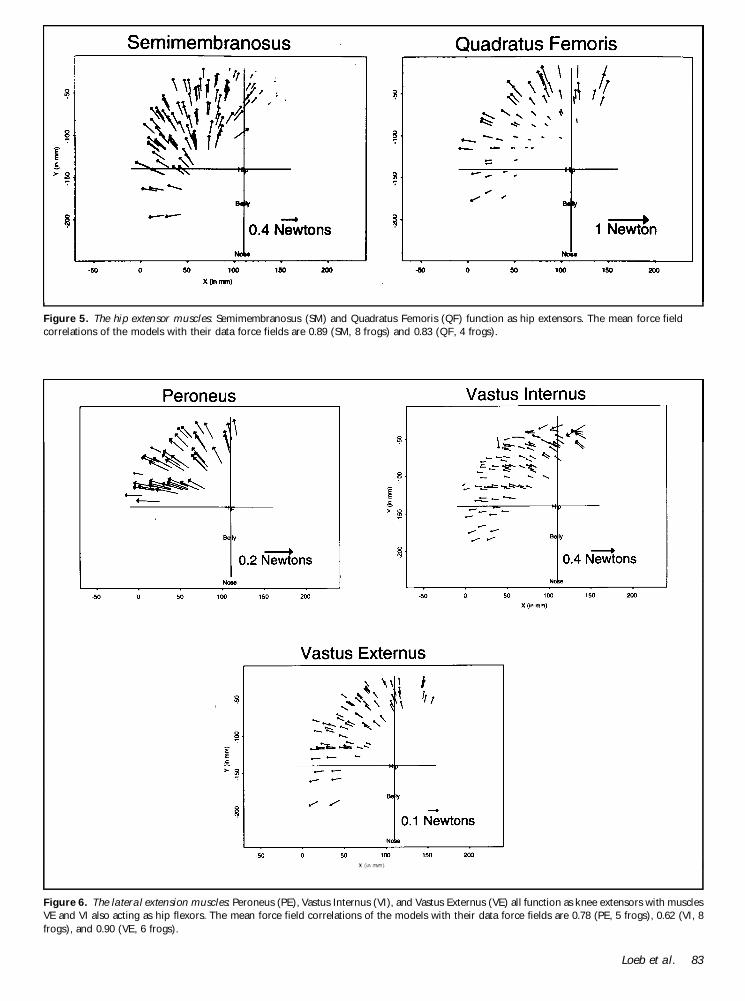