Output-Based Error Estimation and Mesh

Adaptation in Computational Fluid

Dynamics: Overview and Recent Results

Krzysztof J. Fidkowski ∗

University of Michigan, Ann Arbor, MI 48109

David L. Darmofal †

Massachusetts Institute of Technology, Cambridge, MA 02139

Error estimation and control are critical ingredients for improving the reliability

of computational simulations. Adjoint-based techniques can be used to both estimate

the error in chosen solution outputs and to provide local indicators for adaptive re-

finement. This article reviews recent work on these techniques for Computational

Fluid Dynamics (CFD) applications in aerospace engineering. The definition of the

adjoint as the sensitivity of an output to residual source perturbations is used to

derive both the adjoint equation, in fully-discrete and variational formulations, and

the adjoint-weighted residual method for error estimation. Assumptions and ap-

proximations made in the calculations are discussed. Presentation of the discrete

and variational formulations enables a side-by-side comparison of recent work in out-

put error estimation using the finite volume method and the finite element method.

Techniques for adapting meshes using output error indicators are also reviewed. Re-

cent adaptive results from a variety of laminar and Reynolds-averaged Navier-Stokes

applications show the power of output-based adaptive methods for improving the

robustness of CFD computations. However, challenges and areas of additional future

research remain, including computable error bounds and robust mesh adaptation

mechanics.

I Introduction

The accessibility, fast turnaround time, and almost arbitrary test conditions offered by Computational

Fluid Dynamics (CFD) make it an attractive tool in aerospace design. CFD simulations with sophisticated

physical modeling are now used regularly to reduce design cycle costs and to improve final product design.

This prevalence of CFD has been driven by increasing computational power, by improvements in numerical

methods, and by the need to model complex physical phenomena such as transition and turbulence, to the

extent that simulations on general three-dimensional geometries are now routine.

Such powerful simulation capability is a remarkable achievement for CFD, but it also comes with a new

liability: ensuring that the computed solutions are sufficiently accurate, where at the broadest level, accuracy

is measured with respect to the real physical system. Typically, this liability is managed by practitioners

knowledgeable about the assumptions and limitations of the models and discretization. Quantifying the

∗Assistant Professor, Department of Aerospace Engineering, 3029 Francois-Xavier Bagnoud Building, Member AIAA (cor-responding author).

†Associate Department Head / Associate Professor, Department of Aerospace Engineering, Building 33, Room 207. SeniorMember AIAA.

1 of 48

validity of the models used in simulations in reference to actual experiments, a task that may indeed require

expert judgment, is part of ongoing research in the area of uncertainty quantification and validation1–3 and is

beyond the scope of the present review. Instead, this review focuses on estimating numerical errors caused by

finite-dimensional discretizations of continuous systems. In this regard, even very experienced practitioners

cannot reliably quantify the error in a discrete approximation of a complex flowfield. In addition, reliance on

best-practice guidelines for mesh generation and on previous experience is an open-loop solution that leaves

the door open to large amounts of numerical error for computations on novel configurations.

Even for relatively standard simulations, questions arise regarding the robustness with which CFD meth-

ods can accurately compute outputs of interest. An example is the American Institute of Aeronautics and

Astronautics Drag Prediction Workshop (DPW),4–6 in which force and moment outputs for a representative

set of wing-body geometries and flow conditions were compared across codes used in industry, government

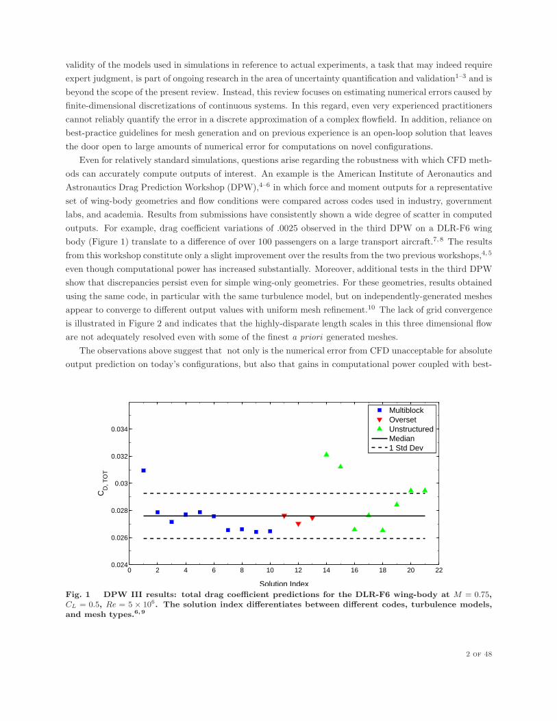
labs, and academia. Results from submissions have consistently shown a wide degree of scatter in computed

outputs. For example, drag coefficient variations of .0025 observed in the third DPW on a DLR-F6 wing

body (Figure 1) translate to a difference of over 100 passengers on a large transport aircraft.7, 8 The results

from this workshop constitute only a slight improvement over the results from the two previous workshops,4, 5

even though computational power has increased substantially. Moreover, additional tests in the third DPW

show that discrepancies persist even for simple wing-only geometries. For these geometries, results obtained

using the same code, in particular with the same turbulence model, but on independently-generated meshes

appear to converge to different output values with uniform mesh refinement.10 The lack of grid convergence

is illustrated in Figure 2 and indicates that the highly-disparate length scales in this three dimensional flow

are not adequately resolved even with some of the finest a priori generated meshes.

The observations above suggest that not only is the numerical error from CFD unacceptable for absolute

output prediction on today’s configurations, but also that gains in computational power coupled with best-

0 2 4 6 8 10 12 14 16 18 20 220.024

0.026

0.028

0.03

0.032

0.034

Solution Index

CD

, TO

T

MultiblockOversetUnstructuredMedian1 Std Dev

Fig. 1 DPW III results: total drag coefficient predictions for the DLR-F6 wing-body at M = 0.75,CL = 0.5, Re = 5 × 10

6. The solution index differentiates between different codes, turbulence models,and mesh types.6,9

2 of 48

Fig. 2 DPW III wing-only results: total, pressure, and skin friction drag convergence for two familiesof grids of two wing geometries, at M = 0.76, α = 0.5o, Re = 5 × 10

6. One set of grids was generatedby Cessna Aircraft Co. and the other by the University of Wyoming. Reproduced with permissionfrom.10

practice expert mesh generation will be insufficient to reliably decrease numerical error to acceptable levels

in the increasingly complex problems of the future. As such, error estimation and control are critical

ingredients for improving the reliability of computational simulations. Control of errors is likely to be done

most efficiently through adaptive methods in which the discretization is iteratively improved through local

mesh refinement and/or increased order of accuracy in regions that most contribute to the solution error. A

key feature of error estimation is the ability to identify such regions.

The general idea of error estimation is not a new concept, and a number of previous works have reviewed

the subject. In the context of error estimates that also provide local indicators, Verfurth analyzes a poste-

riori error estimates for elliptic partial differential equations and shows an equivalence between estimates

based on local residuals and on solutions of local problems.11 Ainsworth and Oden focus on mechanics and

consider a posteriori energy norm error estimates for linear elliptic boundary value problems.12 Johnson et

al note a marked gap between theory and practice in error estimation for CFD, and they derive quantita-

tive discretization error estimates for laminar flows.13, 14 They note that for high Reynolds number flows,

computation of reliable error estimates is difficult because the Navier-Stokes equations become increasingly

ill-conditioned, in that outputs are highly sensitive to initial conditions. Johnson suggests that turbulence

modeling can alleviate this conditioning problem,13 and error estimation for turbulent flows is an ongoing

area of research. Finally, in a recent work, Roy reviews various strategies for using discretization error

estimates to drive mesh adaptation.15

The idea of error estimation has also been deemed important enough to be explicitly addressed by

journals publishing results of numerical computations. In particular, the AIAA journal has a six-point

editorial policy on numerical accuracy. The error estimation methods reviewed in this work are related

primarily to the fourth point in this policy, which concerns the identification of spatial convergence errors.

Currently accepted best-practice guidelines in this regard call for demonstration of mesh convergence using

multiple grids or orders. However, adjoint-based output error estimates could provide an alternative for

quantifying the effect of spatial discretization errors. In addition, although not reviewed in depth in this

work, temporal accuracy can also be addressed through unsteady adjoint methods, and this approach would

address the fifth point in the AIAA editorial policy.

As we describe in this review, adjoint-based techniques can be used to both estimate error in solution

3 of 48

outputs (such as lift and drag) and provide local indicators for adaptive methods. Becker and Rannacher

present a thorough review of the adjoint-weighted residual method for a posteriori error estimation in finite

element discretizations of elliptic, parabolic, and hyperbolic equations.16 In addition, Giles and Pierce17, 18

describe adjoint correction techniques and Giles and Suli19 review a posteriori output error estimation

for finite element methods applied to linear and nonlinear partial differential equations relevant to CFD.

Hartmann and Houston also provide a recent overview of the application of the discontinuous Galerkin

finite element method to output-based adaptation for aerodynamic flows20. Complementing these previous

works, the purpose of this paper is to review output error estimation and mesh adaptation techniques

in the context of aerospace CFD applications and to present a collection of recent results for aerospace

problems. We address output error estimation techniques that are applicable to both finite element and

general discretizations including finite difference and finite volume methods. Fully-discrete and variational

approaches are presented side-by-side to highlight their similarities and differences. Inviscid, laminar, and

Reynolds-averaged Navier-Stokes results for problems including high lift, hypersonic heating, sonic boom,

and launch abort vehicles show the maturity of these methods. We conclude with a presentation of remaining

challenges and ongoing research, which includes a discussion of robust mesh adaptation.

The structure of the paper is as follows. Section II introduces output adjoint solutions for both fully-

discrete and variational problems. Section III then reviews the adjoint-weighted residual method for output-

based error estimation. Error localization and mesh adaptation techniques are reviewed in Section IV.

Section V presents recent implementations and results for aerospace engineering applications. Finally, chal-

lenges and ongoing research are discussed in Section VI.

II Outputs and Adjoints

Since the work of Aubin and Nitsche in a priori optimal order convergence proofs,21 adjoint solutions have

been used in a variety of contexts, ranging from design optimization22–27 to output error estimation.28–41

Adjoint solutions are desirable in all of these contexts for the output sensitivity information that they

provide. Starting from the output-sensitivity property, this section derives the adjoint equations in discrete

and variational formulations.

II.1 Fully-Discrete Formulation

Consider a partial differential equation discretized into Nh, possibly nonlinear, algebraic equations,

Rh(uh) = 0, (1)

where uh ∈ RNh is the vector of unknowns and Rh ∈ R

Nh is the vector of residuals that must be driven to

zero. The subscript h denotes the fineness of the discretization and encompasses both mesh size and approx-

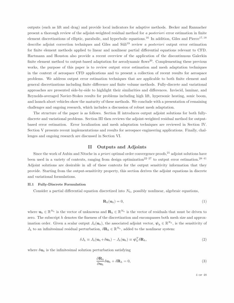
imation order. Given a scalar output Jh(uh), the associated adjoint vector, ψh ∈ RNh , is the sensitivity of

Jh to an infinitesimal residual perturbation, δRh ∈ RNh , added to the nonlinear system:

δJh ≡ Jh(uh+δuh)− Jh(uh) ≡ ψTh δRh, (2)

where δuh is the infinitesimal solution perturbation satisfying

∂Rh

∂uhδuh + δRh = 0, (3)

4 of 48

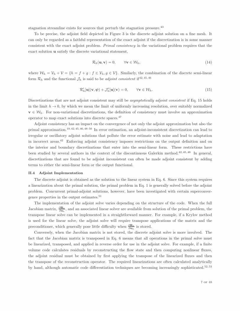
which is obtained by linearizing Eq. 1. The linearization assumes the discrete equations are differentiable.

Further, assuming that the output is also differentiable,

δJh =∂Jh∂uh

δuh = ψTh δRh = −ψTh∂Rh

∂uhδuh, (4)

where Eqs. 2 and 3 were used in the second and third equalities, respectively. In order for Eq. 4 to hold for

all perturbations, we require

∂Jh∂uh

= −ψTh∂Rh

∂uh, (5)

from which ψh must satisfy the discrete adjoint equation

(∂Rh

∂uh

)T

ψh +

(∂Jh∂uh

)T

= 0. (6)

II.2 Variational Formulation

In a variational setting, consider a general semilinear form arising from a Galerkin weighted residual

statement: determine uh ∈ Vh such that

Rh(uh,vh) = 0, ∀vh ∈ Vh, (7)

where Vh is a finite-dimensional space of functions. The subscript h indicates a discretization of the compu-

tational domain, such as a triangulation in a finite element method. Rh(·, ·) : Vh×Vh → R is assumed to be

a semilinear form, linear in the second argument. A scalar output of interest is denoted by Jh(·) : Vh → R,

where the subscript h is included because the output calculation may involve discretization-dependent terms.

Consider an infinitesimal perturbation, δRh(vh), added to the weak statement in Eq. 7, where δRh(·) :

Vh → R. An adjoint ψh ∈ Vh can be defined as the sensitivity of the output to the residual perturbation by

the following relationship:

δJh ≡ Jh(uh+δuh)− Jh(uh) = δRh(ψh). (8)

The infinitesimal state and residual perturbations are related via the statement:

R′

h[uh](δuh,vh) + δRh(vh) = 0, ∀vh ∈ Vh, (9)

where the prime denotes a Frechet linearization with respect to the arguments in the square brackets. Also

linearizing the output,

δJh = J ′

h[uh](δuh) = δRh(ψh) = −R′

h[uh](δuh,ψh), (10)

where Eqs. 8 and 9 were used in the second and third equalities, respectively. For these linearizations to

exist, both the semilinear form and the output are assumed to be differentiable. In order for Eq. 10 to be

5 of 48

true for general perturbations, the adjoint must satisfy the statement: find ψh ∈ Vh such that

R′

h[uh](vh,ψh) + J ′

h[uh](vh) = 0, ∀vh ∈ Vh. (11)

Once a basis is chosen for the weighted residual statements, Eqs. 7 and 11 are equivalent to their discrete

counterparts, Eqs. 1 and 6, respectively. However, the variational formulation is more rigorous for error

estimation, where the concept of a finer solution space is required as discussed in Sections III.2 and III.3.

The construction of such a finer space in the fully-discrete approach requires more information about the

problem, specifically a state prolongation matrix, than just the coarse space discrete system.

II.3 Adjoint Consistency

Eqs. 6 and 11 yield the discrete adjoint ψh, either as a vector or as a function in a finite-dimensional

space. Of interest is how this discrete solution compares to its infinite dimensional (“exact”) counterpart.

Given the exact primal solution, u ∈ V , satisfying

R(u,v) = 0, ∀v ∈ V , (12)

for an appropriately defined space V , the exact adjoint ψ ∈ V satisfies

R′[u](v,ψ) + J ′[u](v) = 0, ∀v ∈ V . (13)

For simplicity, we have assumed that both u and ψ are in V . However, the space for the adjoint solution

does not have to be the same as the space for the primal solution.42

The exact adjoint can be regarded as a Green’s function relating source perturbations in the original

partial differential equation to perturbations in the output.43, 44 To demonstrate this interpretation, a

sample adjoint solution is illustrated in Figure 3 for subsonic flow over a lifting airfoil. Upstream of the

Fig. 3 x−momentum component of the lift adjoint for a NACA 0012 airfoil at M = 0.4, α = 5o. A

positive residual perturbation to the x-momentum equation increases the lift where the adjoint ispositive (red shading) and decreases the lift where the adjoint is negative (blue shading).

airfoil, the adjoint is seen to vary rapidly across the stagnation streamline. This behavior was suggested in

the analysis of Giles and Pierce who found that a square root singularity with respect to distance from the

6 of 48

stagnation streamline exists for sources that perturb the stagnation pressure.43

To be precise, the adjoint field depicted in Figure 3 is the discrete adjoint solution on a fine mesh. It

can only be regarded as a faithful representation of the exact adjoint if the discretization is in some manner

consistent with the exact adjoint problem. Primal consistency in the variational problem requires that the

exact solution u satisfy the discrete variational statement,

Rh(u,v) = 0, ∀v ∈ Wh, (14)

where Wh = Vh + V = {h = f + g : f ∈ Vh, g ∈ V}. Similarly, the combination of the discrete semi-linear

form Rh and the functional Jh is said to be adjoint consistent if42, 45, 46

R′

h[u](v,ψ) + J ′

h[u](v) = 0, ∀v ∈ Wh. (15)

Discretizations that are not adjoint consistent may still be asymptotically adjoint consistent if Eq. 15 holds

in the limit h → 0, by which we mean the limit of uniformly increasing resolution, over suitably normalized

v ∈ Wh. For non-variational discretizations, the definition of consistency must involve an approximation

operator to map exact solutions into discrete spaces.47

Adjoint consistency has an impact on the convergence of not only the adjoint approximation but also the

primal approximation.19, 42, 45, 46, 48–50 In error estimation, an adjoint-inconsistent discretization can lead to

irregular or oscillatory adjoint solutions that pollute the error estimate with noise and lead to adaptation

in incorrect areas.42 Enforcing adjoint consistency imposes restrictions on the output definition and on

the interior and boundary discretizations that enter into the semi-linear form. These restrictions have

been studied by several authors in the context of the discontinuous Galerkin method.42, 45, 48 In general,

discretizations that are found to be adjoint inconsistent can often be made adjoint consistent by adding

terms to either the semi-linear form or the output functional.

II.4 Adjoint Implementation

The discrete adjoint is obtained as the solution to the linear system in Eq. 6. Since this system requires

a linearization about the primal solution, the primal problem in Eq. 1 is generally solved before the adjoint

problem. Concurrent primal-adjoint solutions, however, have been investigated with certain superconver-

gence properties in the output estimates.51

The implementation of the adjoint solve varies depending on the structure of the code. When the full

Jacobian matrix, ∂Rh

∂uh

, and an associated linear solver are available from solution of the primal problem, the

transpose linear solve can be implemented in a straightforward manner. For example, if a Krylov method

is used for the linear solve, the adjoint solve will require transpose applications of the matrix and the

preconditioner, which generally pose little difficulty when ∂Rh

∂uh

is stored.

Conversely, when the Jacobian matrix is not stored, the discrete adjoint solve is more involved. The

fact that the Jacobian matrix is transposed in Eq. 6 means that all operations in the primal solve must

be linearized, transposed, and applied in reverse order for use in the adjoint solve. For example, if a finite

volume code calculates residuals by reconstructing the flow state and then computing nonlinear fluxes,

the adjoint residual must be obtained by first applying the transpose of the linearized fluxes and then

the transpose of the reconstruction operator. The required linearizations are often calculated analytically

by hand, although automatic code differentiation techniques are becoming increasingly sophisticated.52, 53

7 of 48

Multistage and multigrid solution schemes have to be modified to ensure that the asymptotic stability of the

adjoint solver is equal to that of the original primal flow solver.54 Implicit schemes employing point or line

relaxation also have to be modified to preserve discrete duality, as discussed by Nielsen et al .55

Adjoint approximations can also be developed by deriving the adjoint partial differential equations and

then discretizing them. This approach is referred to as the continuous adjoint technique, as opposed to

the discrete adjoint techniques described above. The continuous approach was pioneered for aerospace

applications by Jameson,22 shortly before the discrete approach became popular as well56, 57. No barriers

exist preventing the application of the continuous adjoint method to output error estimation. Indeed in a

recent work, Duraisamy et al 58 compare output error estimation using both the discrete and the continuous

adjoint for the compressible Euler equations. In their results, they find that the discrete adjoint is better

at estimating the fine-space output, while the continuous adjoint is marginally better at estimating the

analytical output when the computational space is well-resolved.

III Error Estimation

III.1 Forms of Error Estimation

The error in a solution can be quantified by various means. Discretization error is the difference between

the discrete solution and the exact solution. Its magnitude is governed by the size of the spatial and temporal

mesh spacings, and it can be measured locally on individual elements or globally under a chosen norm. For

general problems, the exact solution is unknown and the discretization error must be estimated, often using

reconstructions based on smoothness assumptions. Another error estimate relies on the residual, which

is obtained by substituting the approximate solution into the underlying partial differential equation.59–61

Nonzero residuals, calculated point-wise or integrated on an enriched space, indicate regions where the

governing equations are not strongly enforced. Residual error estimates can also be expressed locally or

integrated globally under a norm, although care must be taken in the choice of norm for hyperbolic problems

to prevent uncontrollable growth in the vicinity of a shock.59

Error estimates can be used to define indicators for adaptive refinement of the discretization with the

goal of reducing the error in question. For simulations of predominantly elliptic equations, such as those of

structural elasticity or low-speed flows, adaptive indicators based on local errors are often sufficient.11 How-

ever, many aerospace CFD applications are dominated by convective transport and hence involve equations

of hyperbolic character, for which such estimates lose their efficacy. Zhang et al compare adaptive results

using discretization error and residual indicators for the Euler equations.62, 63 For one-dimensional, subsonic

flows, Zhang et al find that a residual indicator is more efficient compared to a discretization-error indicator

in driving the adaptation to reduce the total solution error. However, for transonic or multi-dimensional

flows, neither indicator is adequately effective. In general, error estimates based on residual or discretization

errors fail to capture propagation effects that are inherent in convection-dominated problems.64 For these

types of problems, the residual and discretization error may not necessarily be large in certain crucial areas

that significantly affect the solution downstream and the computed outputs. For example, for separated

flow over an airfoil, small perturbations in certain upstream areas may have large effects on the location of

the separation point, which in turn has a large effect on the calculated lift and drag. Stated another way,

engineering outputs can be highly sensitive to discretization or residual errors in areas that may not be easily

identifiable a priori.

Output error estimates based on adjoint analysis help to address these problems by quantifying how

8 of 48

residual errors impact the output, accounting for propagation effects in the process. The resulting error

estimate can be used to determine if the engineering output has been computed to sufficient accuracy,

and to drive an adaptive method when the output error is not below a user-specified tolerance. This

section reviews such existing output-error estimation techniques. We begin in Section III.2 by introducing

the adjoint-weighted residual method that connects residuals to output error for variational discretizations.

Then, we show how these techniques can be extended to general discretizations using an algebraic approach in

Section III.3. Finally, Sections III.4-III.6 describe various aspects that impact the practical implementation

of these error estimates including the approximation of fine mesh primal and adjoint states, the effectivity

of error estimates, and the impact of shocks.

III.2 The Adjoint-Weighted Residual Method

Consider a variational solution on a “fine” discretization, uh ∈ Vh, that satisfies Rh(uh,vh) = 0, ∀vh ∈

Vh, and a variational solution on a coarser discretization, RH(uH ,vH) = 0, ∀vH ∈ VH . The discretization

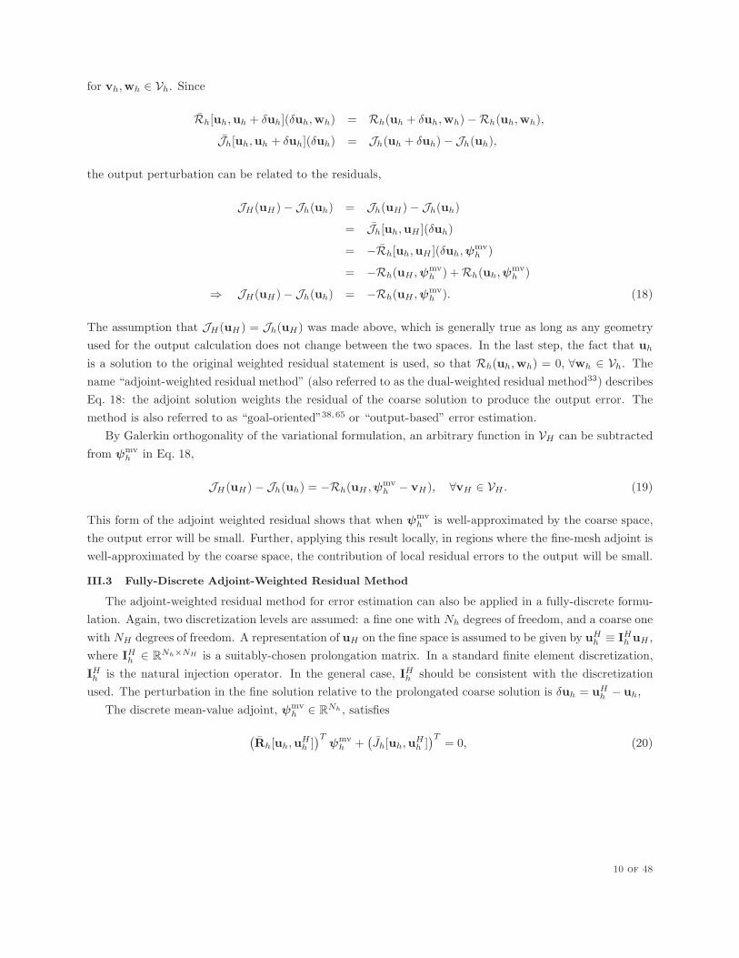
spaces are assumed to be nested, VH ⊂ Vh, so that δuh = uH − uh ∈ Vh. Such a situation is illustrated in

Figure 4 for a one-dimensional finite element solution.

u

x

δuu

u

H h

h

Fig. 4 Comparison in one dimension of a fine solution uh ∈ Vh, a coarse solution uH ∈ VH , and thedifference δuh = uH −uh ∈ Vh. In this example, the solution spaces consist of piecewise linear functionson uniform elements, and Vh is nested in VH with four times as many elements. One coarse elementis shown.

To connect the output error to residuals for finite perturbations, the adjoint equation in Eq. 11 is gen-

eralized using a mean-value linearization.16, 37, 39, 40 Specifically, the mean-value adjoint ψmvh ∈ Vh is the

solution to

Rh[uh,uH ](vh,ψmvh ) + Jh[uh,uH ](vh) = 0, ∀vh ∈ Vh, (16)

where Rh : Vh × Vh → R and Jh : Vh → R are defined by

Rh[uh,uh + δuh](vh,wh) =

∫ 1

0

R′

h[uh + θ δuh](vh,wh) dθ,

Jh[uh,uh + δuh](vh) =

∫ 1

0

J ′

h[uh + θ δuh](vh) dθ, (17)

9 of 48

for vh,wh ∈ Vh. Since

Rh[uh,uh + δuh](δuh,wh) = Rh(uh + δuh,wh)−Rh(uh,wh),

Jh[uh,uh + δuh](δuh) = Jh(uh + δuh)− Jh(uh),

the output perturbation can be related to the residuals,

JH(uH)− Jh(uh) = Jh(uH)− Jh(uh)

= Jh[uh,uH ](δuh)

= −Rh[uh,uH ](δuh,ψmvh )

= −Rh(uH ,ψmvh ) +Rh(uh,ψ

mvh )

⇒ JH(uH)− Jh(uh) = −Rh(uH ,ψmvh ). (18)

The assumption that JH(uH) = Jh(uH) was made above, which is generally true as long as any geometry

used for the output calculation does not change between the two spaces. In the last step, the fact that uh

is a solution to the original weighted residual statement is used, so that Rh(uh,wh) = 0, ∀wh ∈ Vh. The

name “adjoint-weighted residual method” (also referred to as the dual-weighted residual method33) describes

Eq. 18: the adjoint solution weights the residual of the coarse solution to produce the output error. The

method is also referred to as “goal-oriented”38, 65 or “output-based” error estimation.

By Galerkin orthogonality of the variational formulation, an arbitrary function in VH can be subtracted

from ψmvh in Eq. 18,

JH(uH)− Jh(uh) = −Rh(uH ,ψmvh − vH), ∀vH ∈ VH . (19)

This form of the adjoint weighted residual shows that when ψmvh is well-approximated by the coarse space,

the output error will be small. Further, applying this result locally, in regions where the fine-mesh adjoint is

well-approximated by the coarse space, the contribution of local residual errors to the output will be small.

III.3 Fully-Discrete Adjoint-Weighted Residual Method

The adjoint-weighted residual method for error estimation can also be applied in a fully-discrete formu-

lation. Again, two discretization levels are assumed: a fine one with Nh degrees of freedom, and a coarse one

with NH degrees of freedom. A representation of uH on the fine space is assumed to be given by uHh ≡ I

Hh uH ,

where IHh ∈ R

Nh×NH is a suitably-chosen prolongation matrix. In a standard finite element discretization,

IHh is the natural injection operator. In the general case, IHh should be consistent with the discretization

used. The perturbation in the fine solution relative to the prolongated coarse solution is δuh = uHh − uh,

The discrete mean-value adjoint, ψmvh ∈ R

Nh , satisfies

(Rh[uh,u

Hh ]

)Tψmvh +

(Jh[uh,u

Hh ]

)T= 0, (20)

10 of 48

where Rh ∈ RNh×Nh and Jh ∈ R

Nh satisfy

Rh[uh,uh + δuh] =

∫ 1

0

∂Rh

∂uh[uh + θ δuh] dθ,

Jh[uh,uh + δuh] =

∫ 1

0

∂Jh∂uh

[uh + θ δuh] dθ. (21)

Since

Rh[uh,uh + δuh] δuh = Rh(uh + δuh)−Rh(uh),

Jh[uh,uh + δuh] δuh = Jh(uh + δuh)− Jh(uh),

the output perturbation can be related to the residuals,

JH(uH)− Jh(uh) = Jh(uHh )− Jh(uh)

= Jh[uh,uHh ] δuh

= − (ψmvh )

TRh[uh,u

Hh ] δuh

= − (ψmvh )

TRh(u

Hh ) + (ψmv

h )TRh(uh)

⇒ JH(uH)− Jh(uh) = − (ψmvh )

TRh(u

Hh ). (22)

The output for the coarse discretization is assumed to be given by the evaluation of the output on the

fine level discretization using the prolongated solution, i.e. JH(uH) = Jh(uHh ). Further, in the last step,

Rh(uh) = 0 is used.

This adjoint-weighted residual in Eq. 22 can be split into two parts by expressing the mean-value adjoint

on the fine level as a correction from a prolongated coarse adjoint, ψmvh = ψH,mv

h − δψmvh , giving,

JH(uH)− Jh(uh) = −(

ψH,mvh

)T

Rh(uHh )

︸ ︷︷ ︸

computable correction

+(δψmvh )T Rh(u

Hh )

︸ ︷︷ ︸

remaining error

. (23)

ψH,mvh = I

Hh ψ

mvH refers to the prolongated coarse adjoint. The first term, which would be zero due to

Galerkin orthogonality for a variational formulation, is often called the computable correction since it can

be computed without solving the primal or the adjoint on the fine level (only a residual evaluation on the

fine level is required). In particular, it is nonzero for reconstruction-based finite volume schemes. While the

computable correction could be used as an adaptive indicator, previous results indicate that adapting on the

computable correction is not significantly better than heuristic indicators.66, 67 This could be because the

remaining error converges at a higher-order rate so that mesh refinement is more efficient when targeting

this term. Thus, in practice, the approach taken in finite volume applications has been to adapt on the

remaining error while including the computable correction in the estimate of the output.68

III.4 Approximations

Evaluating the output perturbation in Eq. 18 requires a residual evaluation on the fine space Vh, weighted

by the mean-value adjoint, ψmvh (note: the same issues apply to the fully-discrete adjoint-weighted residual

method, but for simplicity we refer only to the variational formulation in this section). A residual evaluation

11 of 48

on Vh is tractable, but solving Eq. 20 to calculate ψmvh requires both a primal and an adjoint solve on Vh.

These calculations on Vh are expensive and defeat the purpose of estimating the error since JH−Jh could be

calculated directly if uh were available. While such an approach can still be useful for obtaining an accurate

indicator for adaptation,65 for error estimates and often for adaptive indicators, approximations are made

to the above formulations.

One approximation is to avoid the mean-value linearization and to estimate the output error with the

following second-order method,

JH(uH)− Jh(uh) = Rh(uH , δψh) +R(2)(||δuh||, ||δψh||), (24)

where δψh ≡ ψH − ψh, ψh is the solution to Eq. 11, and R(2)(||δuh||, ||δψh||) is a remainder term that is

second order in the primal error and δψh. ψH ∈ VH is arbitrary, but to make the remainder term small, it

is chosen as the solution to the coarse adjoint problem,

R′

H [uH ](vH ,ψH) + J ′

H [uH ](vH) = 0, ∀vH ∈ VH . (25)

This approach has been used in both finite element16, 69 and finite volume70, 71 applications. In finite volume

applications, the computable correction must also be included in the error estimate. Becker and Rannacher

show that the error estimate can be improved to third order by including the residual of the adjoint problem,

JH(uH)− Jh(uh) =1

2Rh(uH , δψh) +

1

2Rψh [uH ](δuh,ψH) +R(3)(||δuh||, ||δψh||) (26)

where,

Rψh [uH ](vh,wh) ≡ R′

h[uH ](vh,wh) + J ′

h[uH ](vh), (27)

and R(3)(||δuh||, ||δψh||) is a remainder that is third order in the primal and adjoint error. As with Eq. 24,

this form of error estimate has also been used with both finite element8, 42, 72–74 and finite volume41, 67, 68, 75–81

discretizations.

While the error estimates in Eq. 24 and 26 remove the need for the mean-value linearization, ψh is still

required to determine δψh. In addition, uh is required in Eq. 26 to determine δuh.

One approach for approximating uh is to reconstruct uH on Vh using a higher-accuracy stencil. In the

finite element setting, this could be least squares patch reconstruction.8, 39, 42, 69 Such reconstruction makes

use of a superconvergence property,82, 83 which requires a smoothness assumption that loses validity near

discontinuities. In addition, without limiting, no guarantees exist that reconstructed solutions will remain

physical for nonlinear problems. An alternate approach is therefore to project uH into Vh and to apply

several steps of an iterative solution scheme.73, 74 In either case, the difference between the approximated

uh and uH can be used directly in Eq. 26 to compute the error estimate.

ψh can be approximated in several ways. Just as uh, it can be reconstructed from ψH using a higher-

accuracy stencil.39, 42, 68, 69 In the standard finite volume setting, this reconstruction is typically performed

with quadratic approximation on a uniformly-refined mesh. The least squares problem can be tailored to

penalize first derivative differences, increasing the robustness to oscillations in the presence of under-resolved

or discontinuous features.68 In high-order finite element methods, the reconstruction can be simplified by

12 of 48

using an approximation order increment on the same mesh.42 Reconstruction on a fine space obtained by both

uniform mesh refinement and approximation order increase has also been investigated.84 A disadvantage of

the reconstruction approach is that it does not incorporate physics of the problem, which can be important for

convection-dominated equations. A more robust approach is therefore to solve the adjoint problem exactly

on the chosen fine space,39, 40 although in general this is a costly proposition. We note that for certain highly

non-linear problems, such as turbulent flows, the fine-space adjoint solution can be comparable or cheaper

than the primal solve because the adjoint equations are linear. The particulars of this tradeoff depend on the

solvers used, computing architecture, memory available, and problem-specific factors. When an inexpensive

iterative solver is available, a cheaper alternative is, as in the primal problem, to inject ψH into the fine

space and to apply several steps of the iterative solver, with the linearization based on an approximation

of uh.73, 74 With more effort, the mean-value linearized adjoint, ψmv

h , can be approximated by employing

numerical quadrature in the path integration for the adjoint problem mean-value linearization.39

III.5 Error Effectivity

In the limit of a very fine (and consistent) discretization, “h → 0” and uh → u, Eq. 18 yields the true

output error in the solution: JH(uH) − J (u). In practice, however, a finite dimensional Vh is employed,

obtained from VH by uniform refinement or approximation order increase. Hence, the calculated output

error is generally not equal to and not a bound for the true error. It is an estimate whose accuracy depends

on the enrichment of Vh relative to VH . Indeed, the choice of enrichment governs the behavior of the error

effectivity,

ηeH ≡JH(uH)− Jh(uh)

JH(uH)− J (u). (28)

An effectivity close to 1 is desirable. If H denotes mesh size and the output error converges as JH(uH) −

J (u) = CHHk, a choice of h = H/2 for the enriched space yields an effectivity of ηeH = 1 − (1/2)k. Thus,

even as H → 0, the effectivity does not approach one. Potentially, this underprediction of the true error

could be accounted for if the convergence rate k were known. Another option is to construct the error

estimate using p-enrichment. In this case, the effectivity behaves as ηeH = 1−CkHδk where δk is the increase

in convergence rate of uh relative to uH . Under these assumptions, the effectivity approaches 1 as H → 0.

III.6 Impact of Shocks and Artificial Stabilization

Shock waves (or other under-resolved phenomena) can present a variety of problems when estimating

errors. These problems do not necessarily reflect a breakdown of the error estimation theory, but rather

implementation challenges that occur when employing the enabling approximations. For example, estimation

of uh through reconstruction can introduce oscillations that contaminate error estimates. This contamination

can be reduced by using monotonic reconstruction procedures.

Another issue is the use of shock-capturing stabilization terms in the discretization that are non-zero even

when acting upon the exact solution. In these situations, the semilinear form is inconsistent since RH(u,v)

is not necessarily zero for all v ∈ V . However, for the method to be convergent, the stabilization terms are

assumed to asymptote to zero as H → 0. In other words, the method has asymptotic primal consistency.

The error due to asymptotically consistent stabilization terms can be estimated by separating the weighted

13 of 48

residual statement into consistent and asymptotically consistent parts,

RH(uH ,vH) +RǫH(uH ,vH) = 0, ∀vH ∈ VH . (29)

where RH(·, ·) is a consistent semilinear form, and RǫH(·, ·) is an asymptotically consistent form. Then, using

Eq. 8, the output error due to using asymptotically consistent stabilization is

δJ ǫH = Rǫ

H(uH ,ψH), (30)

where ψH is the solution to Eq. 25, and where the residual perturbation is approximated as infinitesimally

small. When performing error estimation, approximations to uH and ψH are available, and hence δJ ǫH is

computable without a residual calculation on a finer space. Dwight takes advantage of this observation to

efficiently compute the sensitivity of an output to explicitly-added dissipation for finite volume discretizations

of the Euler equations.85 Dwight observes that in many test cases, the artificial dissipation accounts for the

majority of the output error, so that the calculated sensitivity is a good approximation to the output error.

IV Mesh Adaptation

A typical adaptive solution process is illustrated in Figure 5. The input is an initial coarse mesh along

Flow and adjoint solution

Done

Mesh adaptation

Initial coarse mesh & error tolerance

Output error estimate

Error localization

Tolerance

met?

Fig. 5 Adaptive solution process flowchart. The input consists of an initial coarse mesh and arequested error tolerance for a chosen functional. Adaptation stops when the error tolerance is met.

with a user-prescribed error tolerance for an output. The iterative process starts by solving the primal and

adjoint problems on the initial coarse mesh. Next, the output error is estimated using the adjoint-weighted

residual method described in Section III.2. If the global error tolerance criterion is met, the adaptive process

terminates. Otherwise, the error estimate is localized to the elements, and the mesh is adapted. The process

then repeats until the tolerance is met. This process is only valid for the case of one output, although

multiple output functionals can be treated by solving an adjoint for a weighted-sum output,86 a process

that can be augmented with the solution of an error equation to obtain estimates of the individual output

errors.87

In output-based error estimation, the error localization is fairly straightforward. However, numerous

strategies exist for translating the error indicator into a modified mesh. In CFD, the most popular adap-

tation strategy is h-adaptation, in which only the tessellation forming the mesh is varied. In high-order

14 of 48

methods, additional strategies include p-adaptation, in which the approximation order is changed on a fixed

triangulation,42, 88 and hp-adaptation in which both the order and the triangulation are varied.89–98 For CFD

applications, in which solutions often possess localized, singular features, h-adaptation is key to an efficient

adaptation strategy. In addition, most practical codes operate at one or a limited number of orders, making

h-adaptation the only practical approach. With the growing popularity of high-order methods, however,

hp-adaptation will be an important strategy for increased efficiency in the future.

This section reviews general aspects of h-adaptation for CFD. Many of the aspects, especially pertaining

to adaptation mechanics, incorporation of anisotropy, and general optimization strategy, are also relevant to

non-output based adaptation. Additional information on these topics can be found in existing reviews.99–104

The discussion below will focus on aspects of mesh adaptation specifically relevant to output-based error

estimation.

IV.1 Error Localization

The output error estimates in Eqs. 18, 24, and 26 consist of a residual evaluation on the refined space Vh.

In a finite element method, this residual evaluation is a sum over all elements in the fine space. Since the

coarse and fine spaces are assumed nested, Eq. 24 (with an analogous expression for Eq. 18) can be written

as,

JH(uH)− Jh(uh) ≈∑

κH∈TH

∑

κh∈κH

Rh(uH , δψh|κh), (31)

where TH is the coarse triangulation, κH/κh is an element of the coarse/fine triangulation, and |κhrefers to

restriction to element κh. Note that the coarse/fine spaces can consist of the same triangulation, for example

when only the approximation order is increased, in which case κH = κh. Eq. 31 expresses the output error

in terms of contributions from each coarse element. A common approach for obtaining an error indicator is

to take the absolute value of the elemental contribution,16, 19, 39, 40, 68

ǫκH=

∣∣∣

∑

κh∈κH

Rh(uH , δψh|κh)∣∣∣. (32)

When the adjoint residual contribution is used as in Eq. 26, an adjoint error indicator can be defined as

ǫψκH=

∣∣∣

∑

κh∈κH

Rψh [uH ](δuh|κh

,ψH)∣∣∣. (33)

This indicator targets areas of nonzero adjoint residual, weighted by a primal approximation error esti-

mate. Numerical experiments have shown that the two error indicators, ǫκHand ǫψκH

, yield similar mesh

distributions when used to drive adaptation.

The above error localization is applicable to finite volume and discontinuous Galerkin discretizations, since

weighted residuals vanish locally on each element for these discretizations. Thus, no systematic inter-element

error cancellation is expected in the output error estimates and the absolute value signs in Eqs. 32 and 33

are justified. However, local residuals do not necessarily vanish for continuous finite element discretizations.

Consider for example a continuous finite element discretization of Poisson’s equation, in which the elemental

contributions to the residual contain terms of the form∫

κh

∇uH · ∇ψh. Simply placing absolute value signs

around these terms to obtain the elemental error indicator would lead to a systematic over-estimate of the

15 of 48

output error via a sum of the indicators.105 This over-estimate is due to a poor bookkeeping choice for the

error and can be fixed by integrating the residual terms by parts on each element, i.e. by using the primal

residual form45. The result is a set of element-interior terms containing the strong form of the residual,

and a set of face flux jump terms, which are present because the gradient of uH is not continuous. Both of

these terms are expected to go to zero with mesh refinement, and the flux jump terms will dominate for low

orders.106 The face flux residuals can be pushed back onto the elements by assigning half of the flux residual

to each of the two elements adjacent to the face.69 For convection equations, the continuity of uH eliminates

the need for interior flux residuals, although inflow flux residuals are still required and the stabilization terms

must be treated appropriately.36

For systems of equations, indicators are typically computed separately for each equation and summed

together. Due to the absolute values, the sum of the error indicators, ǫ =∑

κHǫκH

, is greater or equal to the

original output error estimate. However, it is not a bound on the actual error, or even on JH(uH)− Jh(uh),

because of the approximations made in the derivation. In practice, the validity of the approximations

improves with refinement, and the above estimate becomes an accurate measure of the true error.

IV.2 h-Adaptation Mechanics

Many approaches to adapting a mesh rely upon the application of local operators through which the

mesh is modified incrementally. A simple example of a local operator is element sub-division in a setting

that supports non-conforming, or hanging, nodes.69, 94, 99, 107, 108 For triangular and tetrahedral meshes,

local mesh modification operators consist of node insertion, face/edge swapping, edge collapsing, and node

movement. These operators have been studied extensively by various authors76, 77, 101, 109–114 in different

contexts. The primary advantage of local operators is their robustness: the entire mesh is not regenerated

all at once, but rather each operator affects only a prescribed number of nodes, edges, or elements.

Another approach to adapting a mesh is global re-meshing, in which a new mesh is generated for the

entire computational domain. The original, or background, mesh is used to store desired mesh characteristics

during re-generation. For applications to adaptation, the desired mesh characteristics are often described

using a Riemannian metric, the idea being that in an optimal mesh, all edge lengths will have unit measure

under the metric.111, 113 In a Cartesian coordinate system of dimension d, an infinitesimal segment δx has

length δΓ under a Riemannian metric M,

δΓ2 = δxT M δx = δxi Mij δxj , (34)

where δxi are the components of δx ∈ Rd, Mij are the components of the symmetric, positive definite metric,

M ∈ Rd×d, and summation is implied on the repeated indices i, j ∈ [1, . . . , d].

The metricM contains information on the desired mesh edge lengths in physical space. AsM is symmetric

and positive definite, the unit measure requirement,

xTM x = 1,

describes an ellipsoid in physical space that maps to a sphere under the action of the metric. The eigenvectors

of M form the orthogonal axes of the ellipsoid – i.e. the principal directions. The corresponding eigenvalues,

16 of 48

λi, are related to the lengths of the axes, hi, via

λi =1

h2i

⇒hihj

=

(λjλi

)1/2

Physically, the hi are the principal stretching magnitudes. A diagram of a possible ellipse resulting from the

unit-measure requirement in two dimensions is given in Figure 6. Thus, the ratio of eigenvalues of M can

e2

h2

e1

h1

Fig. 6 Ellipse representing requested mesh sizes implied by equal measure under a Riemannian met-ric M. Also shown are the principal directions, ei, and the associated principal stretching magnitudes,hi.

be used to define a desired level of anisotropy.

A successful approach for generating simplex meshes based on a Riemannian metric is mapped Delaunay

triangulation, in which a Delaunay mesh generation algorithm104 is applied in the mapped space, allowing for

the creation of stretched and variable-size triangles or tetrahedra.115 This method is implemented in the Bi-

dimensional Anisotropic Mesh Generator (BAMG),116, 117 which has been used in various finite volume41, 118

and discontinuous Galerkin73, 74, 119 applications requiring anisotropic meshes. Examples of output-adapted

meshes obtained using BAMG are shown in Figures 10, 20, and 22.

IV.3 Overview of Adaptation Strategies

In h-adaptation, the determination of which elements to refine or coarsen has important implications for

practical simulations: too little refinement at each adaptation iteration may result in an unnecessary number

of iterations; too much refinement may ask for an expensive solve on an overly-refined mesh. Aftosmis and

Berger discuss adaptation strategies in terms of error distribution histograms,120 in which elements are binned

according to the error indicator (Eq. 32 for output-based adaptation). The assumption made in virtually all

adaptation strategies is that in an ideal mesh the user-prescribed error tolerance is satisfied and the error

is equidistributed among the elements.101 This situation corresponds to a “delta” histogram, in which all

elements lie in the same bin. In contrast, the initial coarse mesh will generally have some distribution of

error indicators, as illustrated in Figure 7. The goal of an adaptation strategy is then to drive the histogram

towards the ideal delta distribution. Note that this characterization of adaptation strategies also holds for

runs in which a maximum element count is specified instead of an error tolerance. The ideal mesh in this

17 of 48

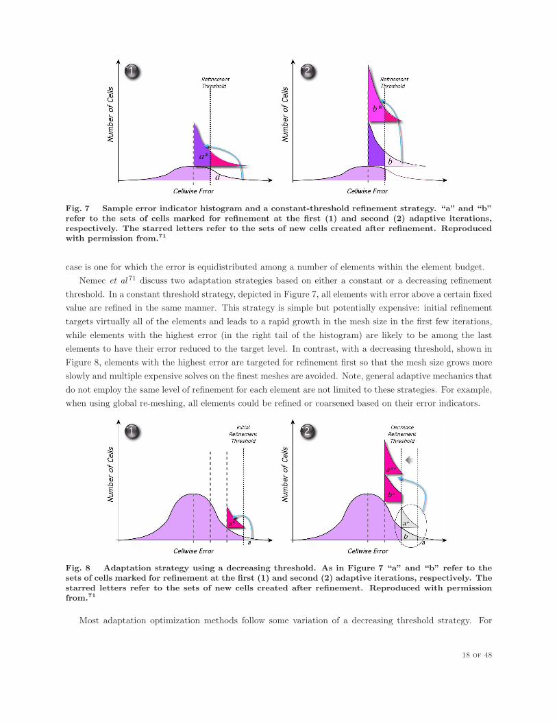
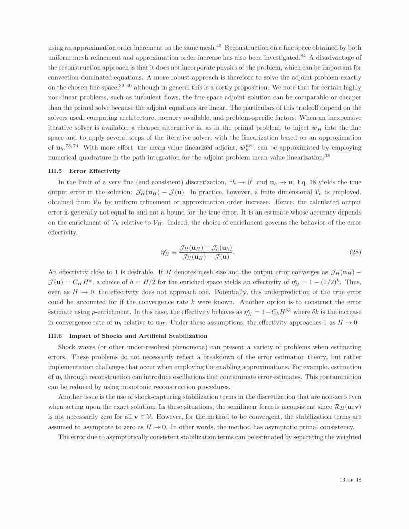
Fig. 7 Sample error indicator histogram and a constant-threshold refinement strategy. “a” and “b”refer to the sets of cells marked for refinement at the first (1) and second (2) adaptive iterations,respectively. The starred letters refer to the sets of new cells created after refinement. Reproducedwith permission from.71

case is one for which the error is equidistributed among a number of elements within the element budget.

Nemec et al 71 discuss two adaptation strategies based on either a constant or a decreasing refinement

threshold. In a constant threshold strategy, depicted in Figure 7, all elements with error above a certain fixed

value are refined in the same manner. This strategy is simple but potentially expensive: initial refinement

targets virtually all of the elements and leads to a rapid growth in the mesh size in the first few iterations,

while elements with the highest error (in the right tail of the histogram) are likely to be among the last

elements to have their error reduced to the target level. In contrast, with a decreasing threshold, shown in

Figure 8, elements with the highest error are targeted for refinement first so that the mesh size grows more

slowly and multiple expensive solves on the finest meshes are avoided. Note, general adaptive mechanics that

do not employ the same level of refinement for each element are not limited to these strategies. For example,

when using global re-meshing, all elements could be refined or coarsened based on their error indicators.

Fig. 8 Adaptation strategy using a decreasing threshold. As in Figure 7 “a” and “b” refer to thesets of cells marked for refinement at the first (1) and second (2) adaptive iterations, respectively. Thestarred letters refer to the sets of new cells created after refinement. Reproduced with permissionfrom.71

Most adaptation optimization methods follow some variation of a decreasing threshold strategy. For

18 of 48

example, a fixed-fraction approach prescribes a fraction of elements with the highest error indicator to be

refined at each adaptation iteration, such that the decreasing threshold is a function of the shape of the error

histogram. Then, the elements targeted for adaptation are typically refined in a locally uniform manner, e.g.

by splitting all edges in half. This simple approach has been applied to output-based adaptation in several

studies33, 39, 40, 65, 70, 98 The fixed-fraction parameter is often chosen heuristically in a trade-off between an

excessive number of iterations and a risk of over-refinement. Nevertheless, the method works quite well for

practical problems.

IV.4 Incorporating a priori Analysis and Anisotropy

The fixed-fraction adaptive strategy with locally uniform refinement does not account for the rate at

which the error decreases with mesh refinement in a given adaptive iteration. This disregard for the error

convergence rate could lead to over-refinement of the mesh or to an excessive number of adaptive iterations

to achieve the desired target error. Adaptation strategies have been developed that attempt to meet the

global tolerance while equidistributing the error among elements through the incorporation of a priori error

analysis. In the context of isotropic, output-based adaptation, Venditti and Darmofal68 developed such a

method based on the previous work of Zienkiewicz and Zhu.121 In this method a permissible element error

eκ = e0/N is defined at each adaptation iteration, where e0 is the user tolerance, and N is the current

number of elements. Coupled with an a priori error estimate that the error converges as O(hr), where r is

the a priori estimated convergence rate, element size requests can be made that equidistribute the error.

An important ingredient in h-adaptation for aerodynamic computations is the ability to generate stretched

elements in areas such as boundary layers, wakes, and shocks, where the solution exhibits anisotropy, which

refers to variations of disparate magnitudes in different directions. While stretched elements can be created

to a limited extent with hanging-node refinement, by optimally choosing the refinement direction,122, 123

unstructured triangular and tetrahedral grids offer the most flexibility in anisotropic refinement. The first

output-based adaptive method to incorporate anisotropy was proposed by Venditti and Darmofal41, 124 and

applied to a nominally second-order accurate finite volume algorithm. Their approach was to combine the

isotropic, output-based approach using a priori estimates with existing Hessian-based methods for anisotropic

adaptation.

For spatially second-order methods, the dominant method for detecting anisotropy involves estimating

the Hessian matrix, H, of a scalar solution, u.111, 113, 115, 125 The components of H are given by

Hij =∂2u

∂xi∂xj, i, j ∈ [1, .., d], d = spatial dimension.

The second derivatives can be estimated by, for example, a quadratic reconstruction of a linear solution. For

the Euler or Navier-Stokes equations, the Hessian of the Mach number has been found to perform sufficiently

well as the scalar u.

The metric is obtained from the Hessian by requiring that the approximation error estimate of the scalar

quantity u be the same in any chosen spatial direction. For linear approximation of u along the segment

δx, the maximum approximation error can be bounded by the second derivative of u along δx. The Hessian

matrix stores precisely this information, so that requiring the approximation error bound to be approximately

19 of 48

constant independent of the direction of δx, leads to the metric choice

M = C|H|, (35)

where C is a constant independent of direction, and |H| is the positive, semi-definite form of the Hessian:

|H| = V|Λ|V−1 for H = VΛV−1. Two intervals, δx1 and δx2, having the same measure under this M will

have the same estimated approximation error bounds.

To fully define the metric, the absolute mesh size, i.e. the constant C in Eq. 35, has to be determined.

While in pure Hessian-based adaptation a global value for C is used, the output-based method of Venditti

and Darmofal sets C locally according to the output error indicator.41 As a result, the smallest mesh length

is controlled by the output error indicator while the anisotropy is controlled by the solution Hessian.

The definition of a metric tensor becomes difficult for high-order methods because the standard Hessian

matrix approach assumes linear approximation of the scalar quantity. For general order p, the approximation

error is governed by the order p + 1 derivatives. One possible extension of the Hessian approach is based

on constructing a metric around the direction of maximum p + 1st derivative.8, 72 In two dimensions, the

anisotropy stretching ratio is set equal to the p+ 1 root of the ratio between this maximum derivative and

the derivative normal to this direction. This approach has the disadvantage of requiring a search over all

directions to determine the maximum p+1 derivative. In three dimensions, the approach would require two

searches and seems impractical. More recently, Pagnutti and Ollivier-Gooch developed a method to calculate

a metric for general p utilizing a Fourier series representation of p+1 order terms.126 This approach appears

to extend to three dimensions quite readily, though to date has not been implemented. Another alternative

to searching for the maximum p + 1 derivative directly is to compute the order p + 1 derivative tensor

that is analogous to the Hessian for p = 1. When adaptation choices are limited, such as for hanging-node

refinement of quadrilateral or hexahedral elements, only the diagonal entries of this tensor are necessary to

make the adaptation decision.127 In addition, for discontinuous solution approximations on quadrilateral or

hexahedral meshes, a surrogate heuristic for the order p+1 derivatives is inter-element jumps in the solution.

Anisotropic adaptation using this jump information has been found to be comparable to using derivative

information for several problems of aerodynamic interest.127

An additional problem with higher-order discretization is the need for curved mesh elements and high-

fidelity geometry representations. Recent work by Oliver74 explores a novel implementation approach for

high-order metric-driven meshing, in which the adaptation is performed on a mapped linear-triangle mesh.

An elasticity analogy is then used to transform the linear mesh to a curved, boundary-conforming mesh

around the true geometry. The robustness of this approach relies on the success of the linear meshing,

which may not be guaranteed for highly-anisotropic boundary-layer meshes. Recently, Persson and Peraire

developed an approach to curved meshes based on a nonlinear elasticity analogy using Lagrangian solid

mechanics.128 This approach appears quite robust, though involves solution of a nonlinear set of equations

to perform the mesh motion.

The metric tensor may also be used to guide an adaptation procedure based on local operators. In the

context of pure Hessian-based adaptation, Diaz et al 111 present a two-dimensional algorithm that uses the

metric-based edge length to decide which operation to apply. Specifically, edge splitting, edge collapsing,

edge swapping, and node movement are applied to make all edges approximately the same length when

measured using the metric tensor. Habashi et al 113, 129, 130 and Xia et al 114 present similar algorithms, with

20 of 48

slight modifications in Hessian definition and in the local operators. Park76, 77 extends these local mesh

modification operators to output-based mesh adaptation, in both two and three dimensions.

IV.5 Direct Optimization Adaptation

The output-based adaptive approaches described in Section IV.4 rely upon a priori analysis to estimate

desired grid characteristics. Further, the approximation error assumptions are made without regard to the

output of interest by using a single scalar, such as the Mach number, to control the anisotropy for a system

of equations. While the Mach number choice has worked well so far, it is arbitrary. Diaz et al 111 propose

choosing an intersection of metrics derived from all variables in the system, although this choice relies on

the variables used (e.g. conservative versus primitive), and using more variables can make the resulting

intersected metric too restrictive. More generally, for output-based adaptation, the assumption that the

directional approximation error must be equidistributed for one or more scalar variables at each point in the

domain may not be valid. Of interest are only the approximation errors that create residuals that affect the

output. This observation has motivated research into adaptation algorithms that more directly target the

error indicator.

Formaggia et al 131–133 combine Hessian-based approximation error estimates with output-based a poste-

riori error analysis to arrive at an output-based error indicator that explicitly includes the anisotropy of each

element. However, for the purpose of mesh adaptation, a metric is still defined using the resulting element

modification requests. In a recent work, Richter derives a posteriori directional output error estimates and

presents an associated anisotropic adaptation strategy for quadrilateral and hexahedral elements134. Schnei-

der and Jimack135 calculate the sensitivities of the output error estimate with respect to node positions

and formulate an optimization problem to reduce the output error estimate by redistributing the nodes.

The sensitivities with respect to node positions are calculated efficiently by solving an additional adjoint

problem. This approach directly targets the output error estimate and automatically leads to anisotropic

meshes where appropriate. Schneider and Jimack then combine this node repositioning with isotropic local

mesh refinement sequentially in a hybrid optimization/adaptation algorithm.

For unstructured meshes, Park81 introduces an algorithm that directly targets the output error through

local mesh operators of element swapping, node movement, element collapse, and element splitting. Using

the output error indicator to rank elements and nodes, these operations are performed in sequence and

automatically result in mesh anisotropy. The details of the adaptation are also given in an earlier work, in

the context of approximation error.136 While the grids produced by this technique lack the regularity of

those produced using metric-based adaptation, their accuracy is comparable. Houston et al 137 also present

a direct optimization approach for output error reduction, using anisotropic discrete refinement options

on quadrilateral elements, an approach which has also been applied to compressible flows20. This idea,

with certain theoretical and implementation modifications, is also extended to aerodynamic simulations on

body-fitted grids in a recent work by Ceze and Fidkowski.138

IV.6 Cut-Cell Methods

A successful adaptation algorithm relies on automation and robustness of the mesh generation or mod-

ification. Standard boundary-conforming meshers must ensure both geometry fidelity and mesh validity, a

task that becomes difficult, for example, for anisotropic meshes around curved geometries. An alternate

approach to mesh generation is based on the idea of cut cells, in which the computational domain is formed

by intersecting the geometry of interest with a volume-filling background mesh. Without the boundary-

21 of 48

conforming constraint, generation or adaptation of the volume-filling background mesh is straightforward.

However, the burden of robustness is transferred to the computational geometry problem of intersecting the

background mesh with the geometry.

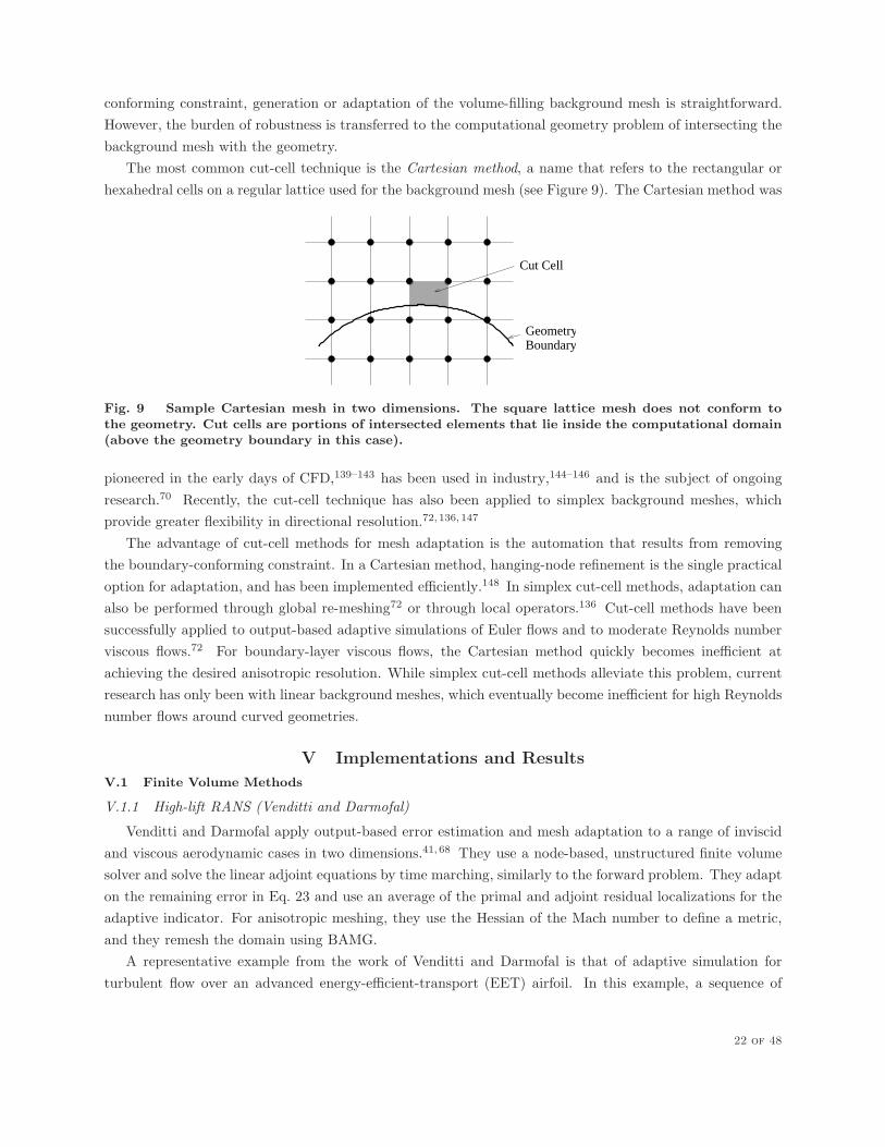
The most common cut-cell technique is the Cartesian method, a name that refers to the rectangular or

hexahedral cells on a regular lattice used for the background mesh (see Figure 9). The Cartesian method was

Cut Cell

GeometryBoundary

Fig. 9 Sample Cartesian mesh in two dimensions. The square lattice mesh does not conform tothe geometry. Cut cells are portions of intersected elements that lie inside the computational domain(above the geometry boundary in this case).

pioneered in the early days of CFD,139–143 has been used in industry,144–146 and is the subject of ongoing

research.70 Recently, the cut-cell technique has also been applied to simplex background meshes, which

provide greater flexibility in directional resolution.72, 136, 147

The advantage of cut-cell methods for mesh adaptation is the automation that results from removing

the boundary-conforming constraint. In a Cartesian method, hanging-node refinement is the single practical

option for adaptation, and has been implemented efficiently.148 In simplex cut-cell methods, adaptation can

also be performed through global re-meshing72 or through local operators.136 Cut-cell methods have been

successfully applied to output-based adaptive simulations of Euler flows and to moderate Reynolds number

viscous flows.72 For boundary-layer viscous flows, the Cartesian method quickly becomes inefficient at

achieving the desired anisotropic resolution. While simplex cut-cell methods alleviate this problem, current

research has only been with linear background meshes, which eventually become inefficient for high Reynolds

number flows around curved geometries.

V Implementations and Results

V.1 Finite Volume Methods

V.1.1 High-lift RANS (Venditti and Darmofal)

Venditti and Darmofal apply output-based error estimation and mesh adaptation to a range of inviscid

and viscous aerodynamic cases in two dimensions.41, 68 They use a node-based, unstructured finite volume

solver and solve the linear adjoint equations by time marching, similarly to the forward problem. They adapt

on the remaining error in Eq. 23 and use an average of the primal and adjoint residual localizations for the

adaptive indicator. For anisotropic meshing, they use the Hessian of the Mach number to define a metric,

and they remesh the domain using BAMG.

A representative example from the work of Venditti and Darmofal is that of adaptive simulation for

turbulent flow over an advanced energy-efficient-transport (EET) airfoil. In this example, a sequence of

22 of 48

a) Lift convergence b) Output (left) and Hessian (right) adapted meshes

Fig. 10 Advanced energy-efficient-transport (EET) airfoil, M∞ = 0.26, α = 8o, Re = 9× 10

6. Compar-ison of lift convergence for output-based and Hessian-based adaptation, and near-field views of thefinal adapted meshes. Note that the output-adapted results agree very well with experiment andother fine-resolution numerical studies. Reproduced with permission from.41

lift-adapted meshes is compared to meshes adapted using only the Hessian of the Mach number with no

output-error information. The resulting convergence of the lift output is shown in Figure 10a. The corrected

output in both runs was calculated using the computable correction in Eq. 23. The improved convergence of

the runs adapted on the output error compared to those adapted on the Hessian is clear. The finest adapted

meshes from both runs are shown in Figure 10b. Note the increased resolution of the output-adapted mesh

near the main-element leading edge and over the upper surface of the main element. Also note that the

Hessian-based mesh predicts the lower slat wake in a different location and does not resolve the flow in the

cavity region of the main element.

V.1.2 Launch Abort Vehicle (Nemec et al )

Nemec et al apply an output-based adaptive framework to a Cartesian, cut-cell, finite-volume code.70, 71

They solve the discrete adjoint equations by marching to steady-state with the same Runge-Kutta scheme

and multigrid solver used for the flow solution. The adjoint solve requires transpose linearizations of the

residual evaluation applied in reverse order, and this process is simplified by freezing the limiter used for the

spatial reconstruction. Details on the adjoint implementation are given in.149

For the fine space Vh in output error estimation, Nemec et al use an embedded grid obtained by uniformly

refining each hexahedral cell in the Cartesian grid. They then obtain an error indicator by weighting the

residual of the coarse, linearly-reconstructed solution on the embedded grid with an adjoint error that is

the difference between piecewise linear and piecewise constant reconstructions of the coarse adjoint solution.

Results in70 compare the performance of this error estimate versus one that employs a more rigorous quadratic

reconstruction of the adjoint and show reduced accuracy of the constant/linear output error estimate but

simpler implementation.

Nemec et al then define a refinement threshold error level for adaptation and at each iteration refine

23 of 48

Fig. 11 Definition of metric components for the LAV model. Reproduced with permission from.71

cells with error above this threshold, using the decreasing threshold strategy described in Section IV.3.

The Cartesian hanging-node adaptation makes use of the robust cut-cell mesh generation capability in

the code,148 allowing for adaptive results with complex geometries. A representative example is that of

aerodynamic analysis of a Launch Abort Vehicle (LAV), illustrated in Figure 11. The output of interest for

this case consists of a linear combination of the normal (N) and axial (A) force coefficients,

J = CN + 0.2CA,

where the weight on the linear combination was determined empirically as one that yielded adequate results

for both forces and moments. Note, the forces and moments are evaluated on the “metric” portion of the

geometry, as specified in Figure 11.

The robustness and automation of the mesh generation process allowed Nemec et al to consider a range

of Mach numbers and angles of attack. A representative case, at M∞ = 1.1, α = −25o, is shown in Figure 12.

Also shown in the figure is a contour plot of the adaptive indicator, where regions shown in gray-scale fall

a) Flow Solution b) Error Indicator

Fig. 12 Launch Abort Vehicle (LAV) Mach number contours, M∞ = 1.1, α = −25o, and the localized

error indicator. Reproduced with permission from.71

below the refinement threshold. Areas marked for refinement include the edges of the heat shield and the

vicinity of the abort motors. Note that only moderate refinement is requested at the shocks, which often

attract excessive refinement with heuristic feature-based indicators.

An example of a final mesh generated by the adaptive process is shown in Figure 13. As expected from

24 of 48

Fig. 13 Initial and adapted meshes for the LAV, at M∞ = 1.1, α = −25o. The initial mesh contains

3,700 cells, while the final mesh after eight adaptation iteration contains almost two million cells.Reproduced with permission from.71

the error indicator, the refinement concentrates on the edges of the heat shield and on the abort motors. The

convergence of the output for this case is shown in Figure 14 on the left. Included on the same plot is the

corrected output, calculated as described in Eq. 23. The right plot in Figure 14 shows the convergence of the

output error estimate. The jump in the error estimate on the final mesh is due to an incompletely-converged

adjoint solution caused by the appearance of small-scale unsteadiness in the primal problem. Nevertheless,

unsteady simulations on the final mesh show that the time-averaged coefficients are in good agreement with

the steady results for this case.71 Note, however, that no benchmark experimental or numerical data are

available to verify the adaptive results for this case.

V.1.3 Sonic Boom (Park)

Park presents output-based, adaptive results for an unstructured, cut-cell finite volume method.81 The

method is node-based, and the cut-cell approach allows for automated mesh generation. Park solves the

linear adjoint equation using a dual-consistent time-marching method54, 55 and adapts on the remaining

error (Eq. 23) using quadratic reconstruction to obtain the fine-space solutions. He adapts on an indicator

computed from the average of the localized primal and adjoint residuals. The tetrahedral grid adaptation

is based on anisotropic local mesh modification operators combined with mesh movement, as described in

Section IV.5.

An example case from Park’s work is shown in Figure 15. The case consists of a delta wing body used

in existing wind tunnel experiments,150 at M∞ = 1.68, α = 0o. Of interest is the pressure signature 3.6

body lengths away from the geometry. Specifically the output consists of an integral of the square of the

pressure deviation from free-stream, taken over the measurement region. The triangular surface mesh in

Figure 15a is the geometry representation that is used in the cut-cell method. The initial background mesh

from which the geometry was cut contained 2,800 control volumes, while the final adapted background mesh

25 of 48

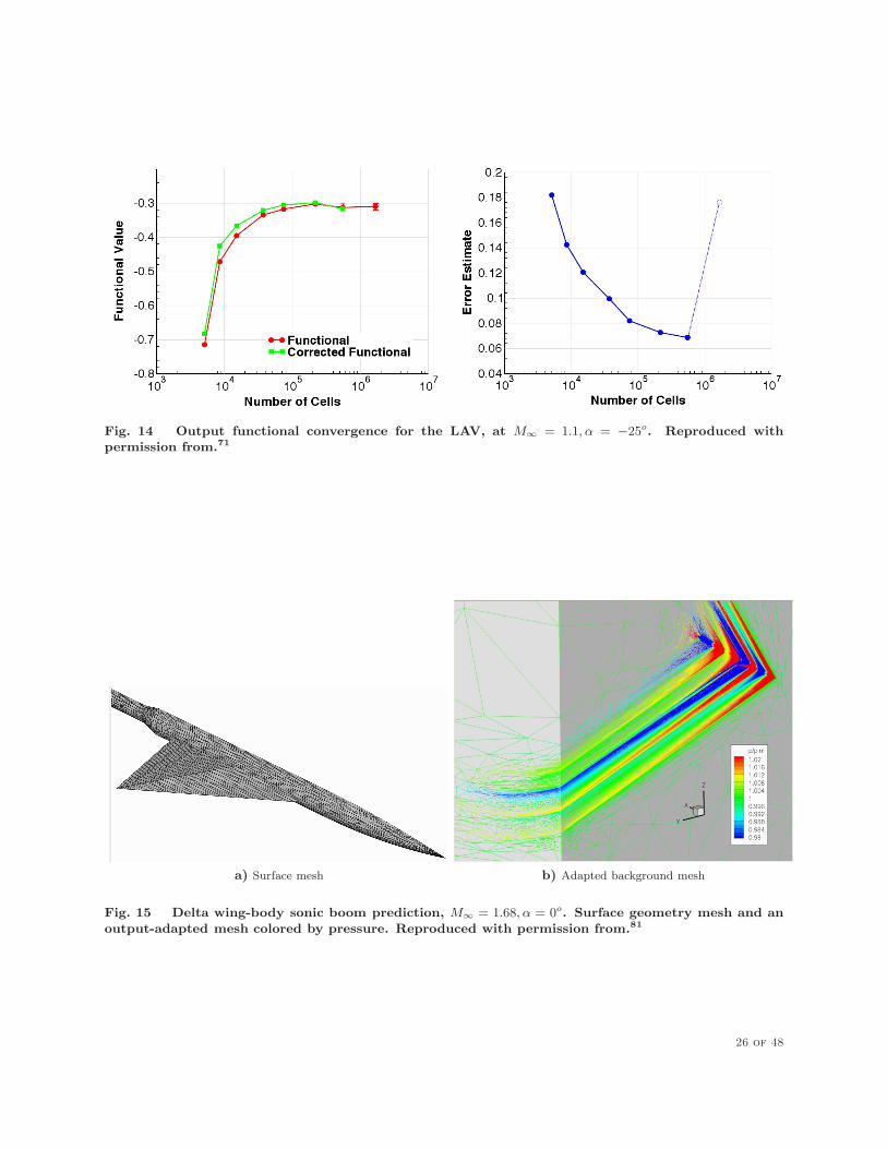
Fig. 14 Output functional convergence for the LAV, at M∞ = 1.1, α = −25o. Reproduced with

permission from.71

a) Surface mesh b) Adapted background mesh

Fig. 15 Delta wing-body sonic boom prediction, M∞ = 1.68, α = 0o. Surface geometry mesh and an

output-adapted mesh colored by pressure. Reproduced with permission from.81

26 of 48

in Figure 15b contained 4.9 million control volumes. Note the alignment of the cells in the final mesh with

the propagated signal.

The adaptation history of the output is shown in Figure 16a, where the error bars denote the remaining

error estimate. Note that the error is severely under-predicted on the very coarse initial meshes. As the

shock is resolved, the error estimate becomes more accurate and begins to decrease in the latter stages of

adaptation. The pressure signature 3.6 body lengths away is shown in Figure 16b. The dotted lines indicate

-6e-05

-4e-05

-2e-05

0

2e-05

4e-05

6e-05

8e-05

1e-04

0.00012

0.00014

1000 10000 100000 1e+06 1e+07

Pre

ssur

e In

tegr

al

Number of Control Volumes

a) Adaptation history

-0.03

-0.02

-0.01

0

0.01

0.02

0.03

-0.2 0 0.2 0.4 0.6 0.8 1 1.2 1.4dp

/p

x/l

Cut Cell Adaptation HistoryCut Cell Final Grid

Wind Tunnel (Digitized from NASA TN D-7160), h/l=3.6, M=1.68

b) Pressure signatures

Fig. 16 Delta wing-body sonic boom prediction, M∞ = 1.68, α = 0o. Pressure integral output history

with error estimates and pressure signature convergence. Reproduced with permission from.81

signatures at intermediate grids during adaptation. The computed signature on the final adapted meshes

agrees well with experimental data.

V.2 Discontinuous Galerkin Methods

V.2.1 Point Error in Transonic Flow (Hartmann and Houston)

Hartmann and Houston compare two types of error indicators for p = 1 discontinuous Galerkin solutions

of the compressible Euler equations.40 The first, type I, indicator is derived from the adjoint-weighted

residual method described in this paper. The second, type II, indicator is an unweighted residual indicator,

in which a priori bounds are placed on the adjoint values, eliminating the need for the adjoint solution.

Adaptive results show the superior performance of using the adjoint-weighted, type I, indicator.

An example case considered by Hartmann and Houston is the converging-diverging nozzle problem shown

in Figure 17. Hartmann and Houston use a damped Newton method to obtain p = 1 primal and adjoint

solutions on a geometry represented by quadratic (q = 2) elements. As the fine space for error estimation,

they use order p = 2 approximation on the same mesh. They adapt the quadrilateral meshes based on the

indicators with fixed-fraction, hanging-node refinement and coarsening. Figure 18 shows adapted meshes

for the two types of error indicators. The type II error indicator, which does not use the adjoint solution,

refines mainly the region near the shock. On the other hand, the type I error indicator leads to refinement

along the characteristics upstream of the point of interest. This targeted refinement yields a lower output

error with fewer degrees of freedom compared to the type II refinement.

Also in this same paper, Hartmann and Houston demonstrated the first application of output-based

27 of 48

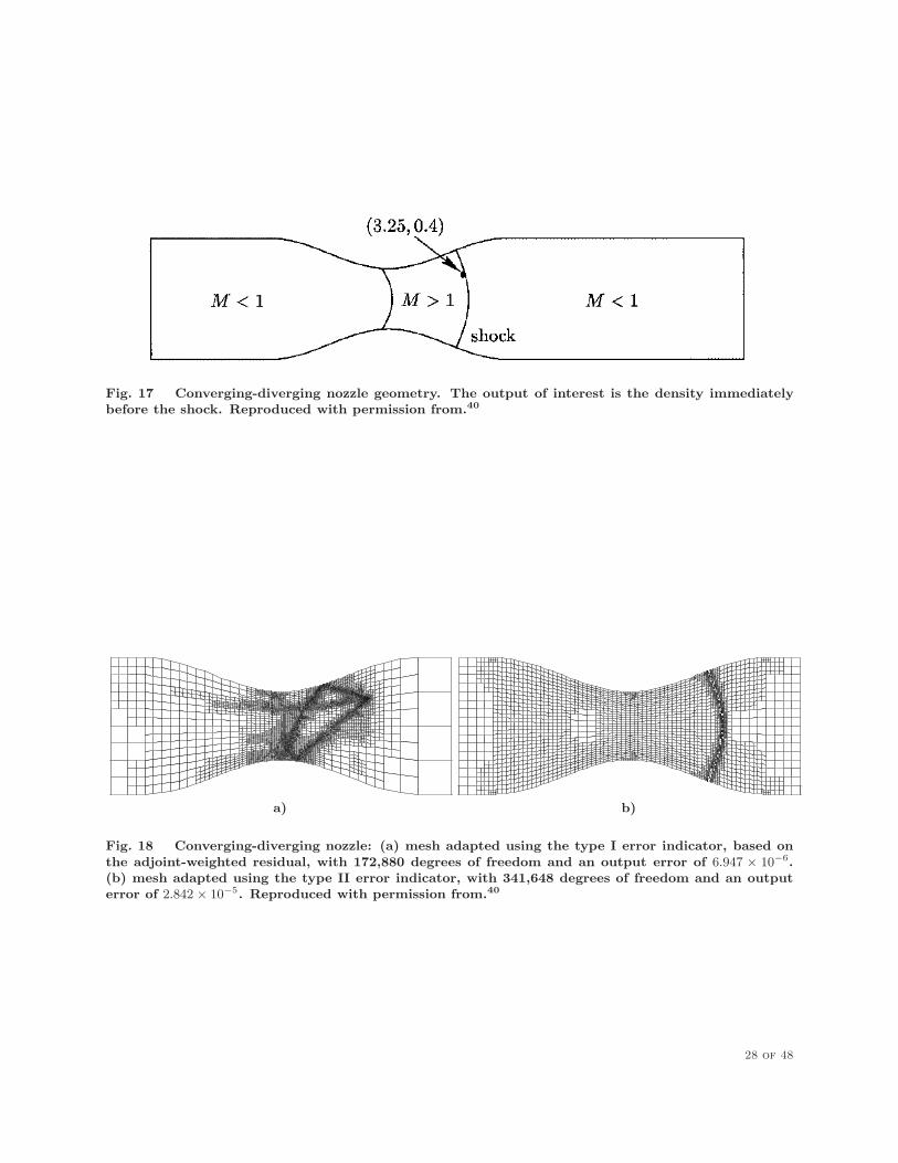
Fig. 17 Converging-diverging nozzle geometry. The output of interest is the density immediatelybefore the shock. Reproduced with permission from.40

a) b)

Fig. 18 Converging-diverging nozzle: (a) mesh adapted using the type I error indicator, based onthe adjoint-weighted residual, with 172,880 degrees of freedom and an output error of 6.947 × 10

−6.(b) mesh adapted using the type II error indicator, with 341,648 degrees of freedom and an outputerror of 2.842 × 10

−5. Reproduced with permission from.40

28 of 48

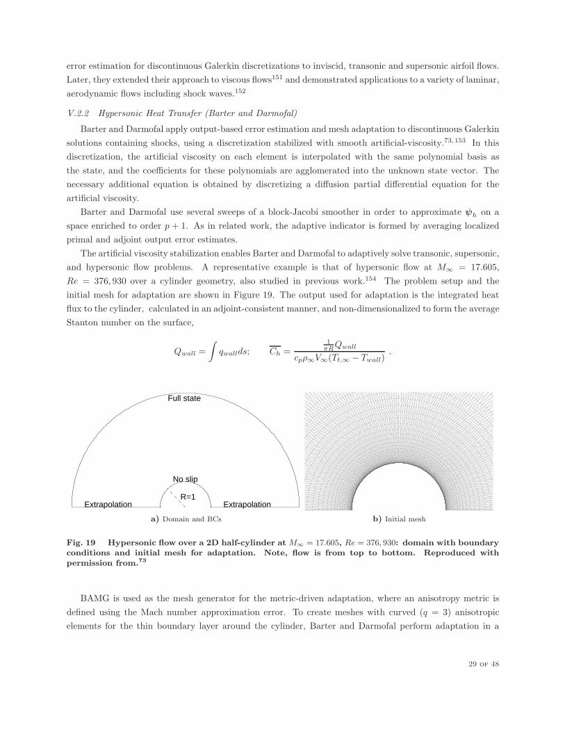
error estimation for discontinuous Galerkin discretizations to inviscid, transonic and supersonic airfoil flows.

Later, they extended their approach to viscous flows151 and demonstrated applications to a variety of laminar,

aerodynamic flows including shock waves.152

V.2.2 Hypersonic Heat Transfer (Barter and Darmofal)

Barter and Darmofal apply output-based error estimation and mesh adaptation to discontinuous Galerkin

solutions containing shocks, using a discretization stabilized with smooth artificial-viscosity.73, 153 In this

discretization, the artificial viscosity on each element is interpolated with the same polynomial basis as

the state, and the coefficients for these polynomials are agglomerated into the unknown state vector. The

necessary additional equation is obtained by discretizing a diffusion partial differential equation for the

artificial viscosity.

Barter and Darmofal use several sweeps of a block-Jacobi smoother in order to approximate ψh on a

space enriched to order p + 1. As in related work, the adaptive indicator is formed by averaging localized

primal and adjoint output error estimates.

The artificial viscosity stabilization enables Barter and Darmofal to adaptively solve transonic, supersonic,

and hypersonic flow problems. A representative example is that of hypersonic flow at M∞ = 17.605,

Re = 376, 930 over a cylinder geometry, also studied in previous work.154 The problem setup and the

initial mesh for adaptation are shown in Figure 19. The output used for adaptation is the integrated heat

flux to the cylinder, calculated in an adjoint-consistent manner, and non-dimensionalized to form the average

Stanton number on the surface,

Qwall =

∫

qwallds; Ch =1πRQwall

cpρ∞V∞(Tt,∞ − Twall).

Extrapolation Extrapolation

No slip

Full state

R=1

a) Domain and BCs b) Initial mesh

Fig. 19 Hypersonic flow over a 2D half-cylinder at M∞ = 17.605, Re = 376, 930: domain with boundaryconditions and initial mesh for adaptation. Note, flow is from top to bottom. Reproduced withpermission from.73

BAMG is used as the mesh generator for the metric-driven adaptation, where an anisotropy metric is

defined using the Mach number approximation error. To create meshes with curved (q = 3) anisotropic

elements for the thin boundary layer around the cylinder, Barter and Darmofal perform adaptation in a

29 of 48

mapped, rectangular space, transforming the requested metric appropriately as described in.74 Figure 20

shows the final adapted mesh for p = 2 and the output convergence history compared to uniform refinement.

The final adapted mesh exhibits refinement in the bow shock, but only to the extent that it impacts the

a) Adapted mesh, p = 2

104

105

106

107

4.74

4.76

4.78

4.8

4.82

4.84

4.86

4.88

4.9x 10

−3

Ave

rage

Stant

on

Numb

er,

Ch

DOF

p=1 Structp=2 Structp=3 Structp=2 Adapt

b) Output convergence

Fig. 20 Hypersonic flow over a 2D half-cylinder at M∞ = 17.605, Re = 376, 930: adaptation onaverage surface Stanton number. Final adapted mesh for p = 2 and output convergence for p = 2

adaptation (“Adapt”) compared to uniform refinement at orders p = 1, 2, 3 (“Struct”). Reproducedwith permission from.73

heat flux on the cylinder. Refinement is also seen in the stagnation streamline, an area to which the heat

flux output is highly sensitive. The convergence history shows that the adapted run converges to an output

within 0.02 percent of the final value with approximately three million degrees of freedom.

V.2.3 Laminar Flows using Simplex Cut Cells (Fidkowski and Darmofal)

Fidkowski and Darmofal use an output-based adaptive indicator to drive cut-cell h-adaptation for a high-

order discontinuous Galerkin discretization of the compressible Navier-Stokes equations.72, 119 They use an

implicit solution procedure for the primal problem that stores the full, compact-stencil, residual linearization,

so that the discrete adjoint solution requires only one transpose application of the same linear solver. The

fine-space adjoint solution ψh is approximated by reconstructing the coarse adjoint, ψH , on the same mesh

with order enriched to p + 1. The adaptive indicator is formed by averaging localized primal and adjoint

output error estimates.

The cut-cell method, illustrated in Figure 21, employs simplex elements and metric-driven global re-

meshing of the background domain to enable automated and anisotropic mesh adaptation. Meshing is

performed using BAMG with anisotropy based on approximation error in the Mach number. Fidkowski and

Darmofal apply the cut-cell adaptive method to several inviscid and viscous flows. A representative example

is that of viscous flow around a NACA 0012 airfoil at M∞ = 0.5, α = 2o, Re = 5, 000. Drag-adapted meshes

for cubic, p = 3, solution approximation are shown in Figure 22 for both the cut-cell method and a boundary-

conforming method. The boundary conforming meshes are generated by curving boundary elements of an

unstructured linear mesh, a process that is susceptible to failure for anisotropic meshes. In both sets of

meshes, areas of refinement include the boundary layer, a large extent of the wake, and, to a lesser extent,

the flow in front of the airfoil.

30 of 48

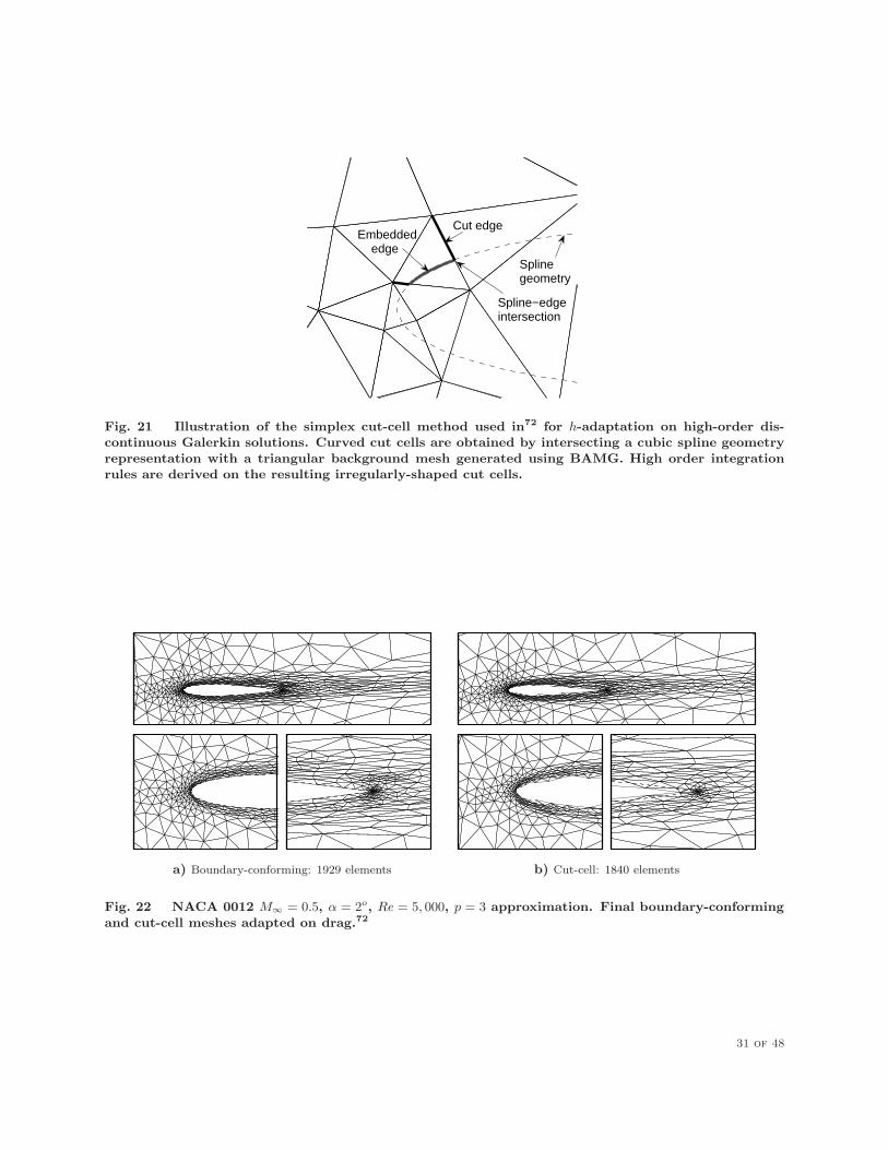
Spline−edgeintersection

Splinegeometry

Cut edgeEmbedded edge

Fig. 21 Illustration of the simplex cut-cell method used in72 for h-adaptation on high-order dis-continuous Galerkin solutions. Curved cut cells are obtained by intersecting a cubic spline geometryrepresentation with a triangular background mesh generated using BAMG. High order integrationrules are derived on the resulting irregularly-shaped cut cells.

a) Boundary-conforming: 1929 elements b) Cut-cell: 1840 elements

Fig. 22 NACA 0012 M∞ = 0.5, α = 2o, Re = 5, 000, p = 3 approximation. Final boundary-conforming

and cut-cell meshes adapted on drag.72

31 of 48

Figure 23 compares adaptive convergence histories of the drag error for approximation orders p = 1, 2, 3.

The boundary-conforming and cut-cell runs converge to the same drag value, and the histories are similar.

In both sets of runs, p = 3 requires only slightly fewer degrees of freedom than p = 2, while p = 1 remains

the most expensive.

103

104

105

10−2

10−1

100

101

102

103

DOF

CD

err

or (

coun

ts)

p = 1p = 2p = 3

a) Boundary-conforming

103

104

105

10−2

10−1

100

101

102

103

DOF

CD

err

or (

coun

ts)

p = 1p = 2p = 3

b) Cut-cell

Fig. 23 NACA 0012 M∞ = 0.5, α = 2o, Re = 5, 000, Drag error versus degrees of freedom for

approximation orders p = 1, 2, 3. Dashed line indicates prescribed tolerance of 0.1 drag counts.72

V.2.4 Multitarget Adaptation (Hartmann)

As discussed in Section IV, the output error estimation framework is designed for one scalar output

quantity. However, in many engineering simulations, multiple scalar outputs are of interest. The presented

framework would require separate adaptive runs, with individual adjoint solutions (auxiliary problems) and

mesh sequences, for each output. To address this issue, Hartmann develops a strategy for multitarget error

estimation and adaptation that only involves one mesh sequence and the solution of two auxiliary problems

at each adaptation iteration87; see also Hartmann and Houston86 for initial work with the inviscid Burgers’

equation. The first auxiliary problem is a linearized error equation that enables the calculation of output

errors for an arbitrary number of outputs. The second auxiliary problem is an adjoint equation for a quantity

that is a weighted-sum of the individual outputs, where the weights can be relative or absolute.

Hartmann compares the multitarget approach to separate adaptations on individual quantities for a

laminar viscous flow discretized with the discontinuous Galerkin method.87 The case is a NACA 0012 airfoil

at M∞ = 0.5, α = 2o, Re = 5, 000. The initial coarse mesh contains 400 quadrilateral elements, and p = 1

solution approximation and hanging-node isotropic mesh refinement are used for all the runs. The adjoint

equations are solved exactly on an enriched p+ 1 space. Figure 24 shows the results of this comparison for

four output quantities: pressure drag coefficient, skin friction drag coefficient, lift coefficient, and moment

coefficient. Prescribed absolute factors were used for the weighted-sum output in this case, with all outputs

weighted using a factor of 1, except for the lift coefficient which was weighted with 1/10. These factors are

based on assumed industrial accuracy requirements, which prescribe tolerances of 5× 10−4 for the drag and

moment coefficients and 5× 10−3 for the lift coefficient.

32 of 48

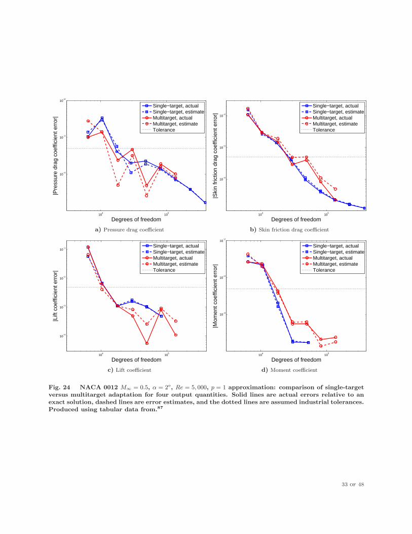
104

105

10−4

10−3

10−2

Degrees of freedom

|Pre

ssur

e dr

ag c

oeffi

cien

t err

or|

Single−target, actualSingle−target, estimateMultitarget, actualMultitarget, estimateTolerance

a) Pressure drag coefficient

104

105

10−4

10−3

10−2

Degrees of freedom|S

kin

fric

tion

drag

coe

ffici

ent e

rror

|

Single−target, actualSingle−target, estimateMultitarget, actualMultitarget, estimateTolerance

b) Skin friction drag coefficient

104

105

10−4

10−3

10−2

10−1

Degrees of freedom

|Lift

coe

ffici

ent e

rror

|

Single−target, actualSingle−target, estimateMultitarget, actualMultitarget, estimateTolerance

c) Lift coefficient

104

105

10−4

10−3

10−2

Degrees of freedom

|Mom

ent c

oeffi

cien

t err

or|

Single−target, actualSingle−target, estimateMultitarget, actualMultitarget, estimateTolerance

d) Moment coefficient

Fig. 24 NACA 0012 M∞ = 0.5, α = 2o, Re = 5, 000, p = 1 approximation: comparison of single-target

versus multitarget adaptation for four output quantities. Solid lines are actual errors relative to anexact solution, dashed lines are error estimates, and the dotted lines are assumed industrial tolerances.Produced using tabular data from.87

33 of 48

The comparison in Figure 24 shows that the multitarget adaptation performs similarly to adaptation on

the individual force outputs, at a reduced cost. Specifically, industry accuracy requirements are satisfied

after the same number of adaptive iterations in each case. The cost reduction of the multitarget approach is

due to solving only two auxiliary problems per adaptation iteration, instead of one adjoint per output, and

to only constructing one mesh sequence. In the present case of four outputs, the compute time reduction was

almost a factor of two. Clearly, the benefit of the multitarget approach improves as the number of output

quantities increases.

V.2.5 Anisotropic Hierarchical Refinement (Leicht and Hartmann)

As described in Section IV.4, Leicht and Hartmann developed a method for anisotropic refinement of

discontinuous Galerkin solutions based on the relative strength of solution jumps across element faces.127

Their implementation begins with a body-aligned mesh of quadrilateral elements. Elements requiring refine-

ment are determined by an adjoint-based error indicator. Then, given these flagged elements, the anisotropy

indicators are calculated for each face. Adaptation occurs either by splitting the flagged element in two

along a particular grid direction or in four along both grid directions depending on the relative strength of

the jump indicators. Hanging nodes are allowed, but with at most one level of refinement difference between

neighboring elements.

More recently, this approach was extended to three-dimensional flows and applied to the DLR-F6 wing-

body geometry using RANS with a k − ω turbulence model.20 To the authors’ knowledge, this was the first

output-based adaptive simulation for 3D RANS using a discontinuous Galerkin method. The surface grid

and the mass adjoint after two adjoint-based refinements targeting the lift coefficient are shown in Figure 25.

VI Challenges and Ongoing Research

While the results shown in the previous section demonstrate the maturity of output-based adaptive

methods, challenges remain in both the practical implementation of these methods and in their theoretical

framework. Some of these are discretization specific, such as investigations into the effects of artificial

stabilization on the accuracy of output error estimates. Others challenges are broader in scope, and these

are reviewed below along with relevant ongoing efforts to address them.

VI.1 Robust Mesh Adaptation

Performing mesh adaptation robustly and efficiently for complex three-dimensional configurations is still

a challenge and an area of ongoing research. The lack of robust and efficient mesh adaptation is probably the

largest barrier limiting the application of output-based adaptation to simple geometries and/or simplified

physics (i.e. inviscid flows as opposed to viscous flows).

The main robustness issue occurs during boundary point insertion on curved geometries: maintaining ge-

ometry fidelity can lead to invalid, negative-volume, elements on the interior, especially for highly-anisotropic

meshes.76 Currently, resolution of such situations is often attempted with iterative application of local op-

erators and local re-meshing.155 However, guaranteed geometric fidelity and element validity in highly

anisotropic meshes around curved geometries has yet to be demonstrated.

Efficient adaptation refers to using available degrees of freedom as effectively as possible. A notable

example of a situation in which efficient adaptation is important is in the resolution of curved, anisotropic,

solution features, as illustrated in Figure 26. Simple isotropic mesh adaptation in these areas, Figure 26a,

wastes resolution in directions where the solution is not changing significantly. In three dimensions, the

34 of 48

a) Adapted surface grid

b) Mass adjoint

Fig. 25 RANS k−ω solution for M = 0.5, Re = 5× 106 flow around the DLR-F6 wing-body geometry

using adjoint-based adaptation targeting lift.20

35 of 48

δ

a) Isotropic

δ

b) Linear anisotropic

δ

c) Curved anisotropic

Fig. 26 Resolution of a thin, curved, anisotropic, two-dimensional layer using various mesh adapta-tion strategies. A resolution length of δ is required normal to the feature, whereas the solution doesnot change much tangentially to the feature. Stretching elements to increase their aspect ratio, definedas the ratio of the largest to smallest element diameters, improves efficiency of the mesh, measuredin terms of degrees of freedom required to resolve the feature. Additionally curving the elementsfurther improves efficiency by alleviating the curvature-imposed geometry resolution constraint.

additional degrees of freedom in the two directions where the solution is not changing quickly make resolution

of thin layers impractical. Stretching elements along these directions helps significantly, especially when the

anisotropic layer is approximately straight. When the layer is curved, however, the maximum feasible aspect

ratio of linear stretched elements is bounded by the curvature of the layer since the geometry must be

resolved, as illustrated in Figure 26b. Efficient resolution of very thin and curved features, such as those

encountered in Reynolds-averaged Navier-Stokes boundary layers, must therefore employ curved elements,

as shown in Figure 26c.

Robust boundary-conforming mesh generation and adaptation techniques currently exist for many ap-

plications requiring only isotropic meshes,156 and such techniques have been successfully applied to drive

output-based adaptation on practical geometries78. An exception here is mesh generation for high-order

methods that require curved elements on geometry boundaries, although in the isotropic case, node move-

ment and certain heuristics are generally sufficient. However, robust boundary-conforming meshing and

adaptation for three-dimensional anisotropic solution features are still areas of ongoing research. Curving

elements for improved efficiency adds another layer of complexity, especially when curved anisotropic features

occur away from the geometry.

Cut-cell techniques eliminate the requirement that the mesh needs to respect the geometry boundary,

and can be robust for complex geometries. However, existing Cartesian methods only allow for isotropic

refinement, except in special cases when the features are aligned with the mesh.71, 148 Simplex cut-cell

methods allow for element stretching, and hence resolution with improved efficiency.72 However, additional

research is required to extend these methods to stretch and curve elements so as to handle curved anisotropic

features in three dimensions.

VI.2 Computable Error Bounds

The output error estimate in Eqs. 18 is not a bound for the true output error in the discrete solution

because of the use of a finite-dimensional fine space, Vh. If the computational mesh is very coarse, the

fine space obtained by uniform mesh refinement or approximation order increase may still be too coarse to

faithfully resolve the output of interest. In such a case, the output error estimate may be severely unreliable.

36 of 48

An example of this effect is the pressure signature adaptation on the delta wing-body sonic boom case

considered by Park, as described in Section V.1.3. The vertical bars in Figure 16a show the pressure integral

error estimate at each adaptation iteration. The relatively small size of the error bars in the first few

iterations indicates that the output error is severely under-predicted on the first meshes. On these meshes

and the fine spaces derived from them, the sonic boom signature is not at all resolved, and the output

error estimate is meaningless. The estimate only becomes accurate after six or seven adaptation iterations,

which corresponds to a substantial increase in the number of degrees of freedom. It does not start dropping

until about ten adaptation iterations. The risk of an inaccurate error estimate on coarse meshes is that an

automated adaptive process may terminate early, without sufficiently resolving the output of interest.

There exists a body of research that addresses this risk through the computation of error bounds on

the outputs of interest.34, 157–161 The goal of this research has been to derive strict, constant-free, lower

and upper bounds for outputs of interest. The bounds calculations are based on a reformulation of the

output calculation into a constrained minimization problem with a convex objective function, with the

model equations entering the problem as equality constraints. Initially, the bounds calculations were strict

with respect to a conservatively refined computational mesh;34, 157, 158 more recently the calculations have

been extended so that the bounds are strict with respect to the exact weak solution of the partial differential

equation.159–161 These calculations rely on the solution of a local adjoint problem that transforms an infinite-

dimensional minimization problem into a finite-dimensional feasibility problem.159

This strategy has been applied to symmetric and non-symmetric coercive problems,157, 159 certain con-

strained and non-coercive problems,34 and also to problems with nonlinear outputs and equations.158, 162, 163

For nonlinear problems, the present procedure yields bounds only for sufficiently resolved meshes, where the

required mesh resolution is not known a priori .158

The bound gap, which is the difference between the upper and lower bounds on the output, can be

separated into positive contributions from each element, yielding an indicator for mesh adaptation. A

strategy that refines elements with a large contribution to the bound gap will efficiently yield a tighter

estimate of the output. The result of applying such a strategy is a solution with fully certifiable precision

of integrated outputs. Additional research in this area is necessary to extend the bounds computations to

additional equation sets, especially for aerospace Computational Fluid Dynamics applications.

VI.3 Unsteady Applications

As output-based adaptation is applied to increasingly complex flows, problems that include unsteadiness

will naturally arise. Even for applications targeting nominally steady solutions, unsteadiness is likely to

occur as wakes are resolved with adaptation. The work of Nemec et al described in Section V.1.2 is an

example of this occurring.

Existing work in the application of adjoint sensitivity analysis to unsteady problems comes largely from

shape optimization research, and ranges from frequency domain methods for periodic unsteady flows164, 165 to

time-accurate continuous and discrete adjoint methods.166–170 Incorporation of time dependence in adjoint

analysis is theoretically a well understood problem. However, the algorithmic issues involved in solving an

unsteady adjoint are substantial as the unsteady adjoint must be marched backward in time from the final

to the initial state. For nonlinear problems, the solution time history must be stored or reconstructed to

build the required Jacobians and output linearizations at each time level.

Mani and Mavriplis apply the adjoint-weighted residual technique to drive time step adaptation in un-

37 of 48

steady flow simulations with deforming meshes.169 For time adaptation, the time step is allowed to vary,

but the spatial mesh distribution is not changed (except for prescribed deformation). The output error is

thus calculated by evaluating the residual of the unsteady primal solution on a finer temporal discretization

and weighting it with the adjoint solution on that discretization. The results in Mani and Mavriplis’s work

indicate a computational savings over uniform temporal refinement for smooth unsteady problems. An area

of future research is combined spatial and temporal adaptation for problems exhibiting non-smooth spatial

and temporal features, where the computational savings of an output-based adaptive method could be very

significant.

VII Acknowledgments

The authors would like to acknowledge M. Aftosmis, G. Barter, R. Hartmann, P. Houston, D. Mavriplis,

M. Nemec, T. Oliver, and M. Park, for permission to present their results and to use their figures. In

addition the authors gratefully acknowledge the support of the Massachusetts Institute of Technology and

the University of Michigan.

References1Oberkampf, W. and T.G.Trucano, “Verification and validation in computational fluid dynamics,”

Progress in Aerospace Sciences , Vol. 38, 2002, pp. 209–272.2Logan, R. and Nitta, C., “Comparing 10 methods for solution verification and linking to model vali-

dation,” Journal of Aerospace Computing, Information, and Communication, Vol. 3, 2006, pp. 354–373.3Eldred, M., Webster, C., and Constantine, P., “Design under uncertainty employing stochastic expan-

sion methods,” AIAA Paper 2008-6001, 2008.4Levy, D. W., Zickuhr, T., Vassberg, J., Agrawal, S., Wahls, R. A., Pirzadeh, S., and Hemsch, M. J.,

“Data summary from the First AIAA Computational Fluid Dynamics Drag Prediction Workshop,” Journal

of Aircraft , Vol. 40, No. 5, 2003, pp. 875–882.5Laflin, K. R., Vassberg, J. C., Wahls, R. A., Morrison, J. H., Brodersen, O., Rakowitz, M., Tinoco,

E. N., and Godard, J.-L., “Summary of data from the second AIAA CFD drag prediction workshop,” AIAA

Paper 2004-0555, 2004.6Frink, N. T., “Test case results from the 3rd AIAA drag prediction workshop,” NASA Langley, 2007,

http://aaac.larc.nasa.gov/tsab/cfdlarc/aiaa-dpw/ Workshop3/final results jm.tar.gz.7Vassberg, J. C., DeHaan, M. A., and Sclafani, T. J., “Grid generation requirements for accurate drag

predictions based on OVERFLOW calculations,” AIAA Paper 2003-4124, 2003.8Fidkowski, K. J., A Simplex Cut-Cell Adaptive Method for High–order Discretizations of the Com-

pressible Navier-Stokes Equations , Ph.D. thesis, Massachusetts Institute of Technology, Cambridge, Mas-

sachusetts, 2007.9Morrison, J. H. and Hemsch, M. J., “Statistical analysis of CFD solutions from the third AIAA drag

prediction workshop,” AIAA Paper 2007-254, 2007.10Mavriplis, D. J., “Results from the 3rd drag prediction workshop using the NSU3D unstructured mesh

solver,” AIAA Paper 2007-256, 2007.11Verfurth, R., “A posteriori error estimation and adaptive mesh-refinement techniques,” Journal of

Computational and Applied Mathematics , Vol. 50, 1994, pp. 67–83.

38 of 48

12Ainsworth, M. and Oden, J. T., “A posteriori error estimation in finite element analysis,” Computer

Methods in Applied Mechanics and Engineering, Vol. 142, 1997, pp. 1–88.13Johnson, C., “On computability and error control in CFD,” International Journal for Numerical

Methods in Fludis , Vol. 20, 1995, pp. 777–788.14Johnson, C., Rannacher, R., and Boman, M., “Numerics and hydrodynamic stability: Toward error

control in computational fluid dynamics,” SIAM Journal on Numerical Analysis , Vol. 32, No. 4, 1995,

pp. 1058–1079.15Roy, C. J., “Strategies for driving mesh adaptation in CFD,” AIAA Paper 2009-1302, 2009.16Becker, R. and Rannacher, R., “An optimal control approach to a posteriori error estimation in finite

element methods,” Acta Numerica, edited by A. Iserles, Cambridge University Press, 2001, pp. 1–102.17Giles, M. and Pierce, N., “Adjoint error correction for integral outputs,” Lecture Notes in Computa-

tional Science and Engineering: Error Estimation and Adaptive Discretization Methods in Computational

Fluid Dynamics , Vol. 25, Springer, Berlin, 2002.18Pierce, N. A. and Giles, M. B., “Adjoint and defect error bounding and correction for functional

estimates,” Journal of Computational Physics , Vol. 200, No. 2, 2004, pp. 769–794.19Giles, M. B. and Suli, E., “Adjoint methods for PDEs: a posteriori error analysis and postprocessing

by duality,” Acta Numerica, Vol. 11, 2002, pp. 145–236.20Hartmann, R. and Houston, P., “Error estimation and adaptive mesh refinement for aerodynamic

flows,” 36th CFD/ADIGMA course on hp-adaptive and hp-multigrid methods: VKI Lecture Series 2010-01

(Oct. 26-30, 2009), edited by H. Deconinck, Von Karman Institute for Fluid Dynamics, 2010.21Strang, G. and Fix, G. J., An Analysis of the Finite Element Method , Wellesley-Cambridge Press,

1988.22Jameson, A., “Aerodynamic design via control theory,” Journal of Scientific Computing, Vol. 3, 1988,

pp. 233–260.23Anderson, W. K. and Venkatakrishnan, V., “Aerodynamic design optimization on unstructured grids

with a continuous adjoint formulation,” Tech. Rep. Report 97-9, ICASE, 1997.24Elliott, J. and Peraire, J., “Practical three-dimensional aerodynamic design and optimization using

unstructured meshes,” AIAA Journal , Vol. 35, No. 9, 1997, pp. 1479–1485.25Nielsen, E. and Anderson, W., “Aerodynamic design optimization on unstructured meshes using the

Navier-Stokes equations,” AIAA Journal , Vol. 37, No. 11, 1999, pp. 1411–1419.26Mohammadi, B. and Pironneau, O., “Mesh adaption and automatic differentiation in a CAD-free

framework for optimal shape design,” International Journal for Numerical Methods in Fluids , Vol. 30, 1999,

pp. 127–136.27Martins, J. R., Alonso, J. J., and Reuther, J. J., “A coupled-adjoint sensitivity analysis method for

high-fidelity aero-structural design,” Optimization and Engineering, Vol. 6, 2005, pp. 33–62.28Babuska, I. and Rheinboldt, W., “A posteriori error estimates for the finite element method,” Inter-

national Journal for Numerical Methods in Engineering, Vol. 12, 1978, pp. 1597–1615.29Babuska, I. and Miller, A., “The post-processing approach in the finite element method – part 1: cal-

culation of displacements, stresses and other higher derivatives of the displacements,” International Journal

for Numerical Methods in Engineering, Vol. 20, 1984, pp. 1085–1109.

39 of 48

30Babuska, I. and Miller, A., “The post-processing approach in the finite element method – part 2: the

calculation of stress intensity factors,” International Journal for Numerical Methods in Engineering, Vol. 20,

1984, pp. 1111–1129.31Giles, M., Larson, M. G., Levenstam, J. M., and Suli, E., “Adaptive error control for finite element

approximations of the lift and drag coefficients in viscous flow,” Tech. Rep. Technical Report NA 76/06,

Oxford University Computing Lab Numerical Analysis Group, 1997.32Monk, P. and Suli, E., “The adaptive computation of far-field patterns by a posteriori error estimation

of linear functional,” SIAM Journal on Numerical Analysis , Vol. 36, No. 1, 1998, pp. 251–274.33Becker, R. and Rannacher, R., “A feed-back approach to error control in finite element methods: Basic

analysis and examples,” East-West Journal of Numerical Mathematics , Vol. 4, 1996, pp. 237–264.34Peraire, J. and Patera, A., “Asymptotic a posteriori finite element bounds for the outputs of non-

coercive problems: the Helmholtz and Burgers equation,” Computer Methods in Applied Mechanics and

Engineering, Vol. 171, 1999, pp. 77–86.35Giles, M. B. and Pierce, N. A., “Improved lift and drag estimates using adjoint Euler equations,” ,

No. 99-3293, 1999.36Houston, P., Rannacher, R., and Suli, E., “A posteriori error analysis for stabilised finite element

approximations of transport problems,” Computer Methods in Applied Mechanics and Engineering, Vol. 190,

2000, pp. 1483–1508.37Pierce, N. A. and Giles, M. B., “Adjoint recovery of superconvergent functionals from PDE approxi-

mations,” SIAM Review , Vol. 42, No. 2, 2000, pp. 247–264.38Oden, J. and Prudhomme, S., “Goal-oriented error estimation and adaptivity for the finite element

method,” Computers and Mathematics with Applications , Vol. 41, 2001, pp. 735–756.39Barth, T. and Larson, M., “A posteriori error estimates for higher order Godunov finite volume

methods on unstructured meshes,” Finite Volumes for Complex Applications III , edited by R. Herban and

D. Kroner, Hermes Penton, London, 2002, pp. 41–63.40Hartmann, R. and Houston, P., “Adaptive discontinuous Galerkin finite element methods for the

compressible Euler equations,” Journal of Computational Physics , Vol. 183, No. 2, 2002, pp. 508–532.41Venditti, D. A. and Darmofal, D. L., “Anisotropic grid adaptation for functional outputs: application

to two-dimensional viscous flows,” Journal of Computational Physics , Vol. 187, No. 1, 2003, pp. 22–46.42Lu, J., An a Posteriori Error Control Framework for Adaptive Precision Optimization Using Discon-

tinuous Galerkin Finite Element Method , Ph.D. thesis, Massachusetts Institute of Technology, Cambridge,

Massachusetts, 2005.43Giles, M. B. and Pierce, N. A., “Adjoint equations in CFD: duality, boundary conditions and solution

behavior,” AIAA Paper 97-1850, 1997.44Giles, M. and Pierce, N., “Analytic adjoint solutions for the quasi-one-dimensional Euler equations,”

Journal of Fluid Mechanics , Vol. 426, 2001, pp. 327–345.45Hartmann, R., “Adjoint consistency analysis of discontinuous Galerkin discretizations,” SIAM Journal

on Numerical Analysis , Vol. 45, No. 6, 2007, pp. 2671–2696.46Oliver, T. A. and Darmofal, D. L., “Impact of turbulence model irregularity on high–order discretiza-

tions,” AIAA Paper 2009-953, 2009.

40 of 48

47Despres, B., “Lax theorem and finite volume schemes,” Mathematics of Computation, Vol. 73, No.

247, 2003, pp. 1203–1234.48Arnold, D. N., Brezzi, F., Cockburn, B., and Marini, L. D., “Unified analysis of discontinuous Galerkin

methods for elliptic problems,” SIAM Journal on Numerical Analysis , Vol. 39, No. 5, 2002, pp. 1749–1779.49Harriman, K., Houston, P., Senior, B., and Suli, E., “hp-version discontinuous Galerkin methods with

interior penalty for partial differential equations with nonnegative characteristic form.” Tech. Rep. Technical

Report NA 02/21, Oxford University Computing Lab Numerical Analysis Group, 2002.50Harriman, K., Gavaghan, D., and Suli, E., “The importance of adjoint consistency in the approxi-

mation of linear functionals using the discontinuous Galerkin finite element method,” Tech. Rep. Technical

Report NA 04/18, Oxford University Computing Lab Numerical Analysis Group, 2004.51Lu, J. and Darmofal, D. L., “A quasi-minimal residual method for simultaneous primal-dual solutions

and superconvergent functional estimates,” SIAM Journal on Scientific Computing, Vol. 24, No. 5, 2003,

pp. 1693–1709.52Muller, J. and Cusdin, P., “On the performance of discrete adjoint CFD codes using automatic differ-

entiation,” International Journal for Numerical Methods in Fluids , Vol. 47, No. 8–9, 2005, pp. 939–945.53Mader, C. A., Martins, J. R., Alonso, J. J., and van der Weide, E., “ADjoint: An approach for the

rapid development of discrete adjoint solvers,” AIAA Journal , Vol. 46, No. 4, 2008, pp. 863–873.54Giles, M. B., Duta, M. C., Muller, J.-D., and Pierce, N. A., “Algorithm developments for discrete

adjoint methods,” AIAA Journal , Vol. 41, No. 2, 2003, pp. 198–205.55Nielsen, E. J., Lu, J., Park, M. A., and Darmofal, D. L., “An implicit, exact dual adjoint solution

method for turbulent flows on unstructured grids,” Computers and Fluids , Vol. 33, 2004, pp. 1131–1155.56Shubin, G. and Frank, P., “A comparison of two closely-related approaches to aerodynamic design

optimization,” Third International Conference on Inverse Design Concepts and Optimization in Engineering

Sciences , edited by G. Dulikravich, Washington D.C., October 23-25 1991.57Beux, F. and Dervieux, A., “Exact-gradient shape optimization of a 2-D Euler flow,” Finite Elements

in Analysis and Design, Vol. 12, 1992, pp. 281–302.58Duraisamy, K., Alonso, J., Palacios, F., and Chandrashekar, P., “Error estimation for high speed flows

using continuous and discrete adjoints,” AIAA Paper 2010-128, 2010.59Sonar, T., “Strong and weak norm refinement indicators based on the finite element residual for

compressible flow computation,” Impact of Computing in Science and Engineering, Vol. 5, 1993, pp. 111–

127.60Sonar, T., Hanneman, V., and Hempel, D., “Dynamic adaptivity and residual control in unsteady

compressible flow computation,” Mathematical and Computer Modelling, Vol. 20, No. 10, 1994, pp. 201–213.61Thomas, I. and Sonar, T., “On a second order residual estimator for numerical schemes for nonlinear

hyperbolic conservation laws,” Journal of Computational Physics , Vol. 171, No. 1, 2001, pp. 227–242.62Zhang, X. D., Pelletier, D., Trepanier, J.-Y., and Camarero, R., “Error control and mesh adaptation

for the Euler equations,” AIAA Paper 2001-0441, 2001.63Zhang, X. D., Vallet, M.-G., Dompierre, J., Labbe, P., Pelletier, D., Trepanier, J.-Y., Camarero, R.,

Lassaline, J. V., Manzano, L. M., and Zingg, D. W., “Mesh adaptation using different error indicators for

the Euler equations,” AIAA Paper 2001-2549, 2001.

41 of 48

64Houston, P. and Suli, E., “Error estimation and adaptive discretization methods in computational

fluid dynamics,” Error Estimation and Adaptive Discretization Methods in Computational Fluid Dynamics ,

edited by T. Barth and H. Deconinck, Springer-Verlag, Heidelberg, Lecture Notes in Computational Science

and Engineering Vol 25, 2002, pp. 269–344.65Solın, P. and Demkowicz, L., “Goal-oriented hp-adaptivity for elliptic problems,” Computer Methods

in Applied Mechanics and Engineering, Vol. 193, 2004, pp. 449–468.66Muller, J. D. and Giles, M. B., “Solution adaptive mesh refinement using adjoint error analysis,”

AIAA Paper 2001-2550, 2001.67Balasubramanian, R. and Newman III, J., “Adjoint-based error estimation and grid adaptation for

functional outputs: Application to two-dimensional, inviscid, incompressible flows,” Computers and Fluids ,

Vol. 38, 2009, pp. 320–332.68Venditti, D. A. and Darmofal, D. L., “Grid adaptation for functional outputs: application to two-

dimensional inviscid flows,” Journal of Computational Physics , Vol. 176, No. 1, 2002, pp. 40–39.69Rannacher, R., “Adaptive Galerkin finite element methods for partial differential equations,” Journal

of Computational and Applied Mathematics , Vol. 128, 2001, pp. 205–233.70Nemec, M. and Aftosmis, M. J., “Error estimation and adpative refinement for embedded-boundary

Cartesian meshes,” AIAA Paper 2007-4187, 2007.71Nemec, M., Aftosmis, M. J., and Wintzer, M., “Adjoint-based adaptive mesh refinement for complex

geometries,” AIAA Paper 2008-0725, 2008.72Fidkowski, K. J. and Darmofal, D. L., “A triangular cut-cell adaptive method for high-order dis-

cretizations of the compressible Navier-Stokes equations,” Journal of Computational Physics , Vol. 225, 2007,

pp. 1653–1672.73Barter, G. E., Shock Capturing with PDE-Based Artificial Viscosity for an Adaptive Higher–Order

Discontinuous Galerkin Finite Element Method , Ph.D. thesis, Massachusetts Institute of Technology, Cam-

bridge, Massachusetts, 2008.74Oliver, T. A., A High–order, Adaptive, Discontinuous Galerkin Finite Elemenet Method for the

Reynolds-Averaged Navier-Stokes Equations , Ph.D. thesis, Massachusetts Institute of Technology, Cam-

bridge, Massachusetts, 2008.75Venditti, D. A. and Darmofal, D. L., “Adjoint error estimation and grid adaptation for functional

outputs: Application to quasi-one-dimensional flow,” Journal of Computational Physics , Vol. 164, No. 1,

2000, pp. 204–227.76Park, M. A., “Adjoint-based, three-dimensional error prediction and grid adaptation,” AIAA Paper

2002-3286, 2002.77Park, M. A., “Three–dimensional turbulent RANS adjoint–based error correction,” AIAA Paper 2003-

3849, 2003.78Lee-Rausch, E. M., Park, M. A., Jones, W. T., Hammond, D. P., and Nielsen, E. J., “Application

of parallel adjoint-based error estimation and anisotropic grid adaptation for three-dimensional aerospace

configurations,” AIAA Paper 2005-4842, 2005.79Jones, W. T., Nielsen, E. J., and Park, M. A., “Validation of 3d adjoint based error estimation and

mesh adaptation for sonic boom predictions,” AIAA Paper 2006-1150, 2006.

42 of 48

80Balasubramanian, R. and Newman III, J., “Comparison of adjoint-based and feature-based grid

adaptation for functional outputs,” International Journal for Numerical Methods in Fluids , Vol. 53, 2007,

pp. 1541–1569.81Park, M. A., Anisotropic Output-Based Adaptation with Tetrahedral Cut Cells for Compressible Flows ,

Ph.D. thesis, Massachusetts Institute of Technology, Cambridge, Massachusetts, 2008.82Zienkiewicz, O. C. and Zhu, J. Z., “The superconvergent patch recovery and a posteriori error es-

timates. Part 1: The recovery technique,” International Journal for Numerical Methods in Engineering,

Vol. 33, 1992, pp. 1331–1364.83Zienkiewicz, O. C. and Zhu, J. Z., “The superconvergent patch recovery and a posteriori error esti-

mates. Part 2: Error estimates and adaptivity,” International Journal for Numerical Methods in Engineering,

Vol. 33, 1992, pp. 1365–1382.84Fidkowski, K. J. and Darmofal, D. L., “Output-based adaptive meshing using triangular cut cells.”

M.I.T. Aerospace Computational Design Laboratory Report. ACDL TR-06-2, 2006.85Dwight, R. P., “Heuristic a posteriori estimation of error due to dissipation in finite volume schemes

and application to mesh adaptation,” Journal of Computational Physics , Vol. 227, 2008, pp. 2845–2863.86Hartmann, R. and Houston, P., “Goal-oriented a posteriori error estimation for multiple target

functionals,” Hyperbolic Problems: Theory, Numerics, Applications , edited by T. Hou and E. Tadmor,

Springer-Verlag, 2003, pp. 579–588.87Hartmann, R., “Multitarget error estimation and adaptivity in aerodynamic flow simulations,” SIAM

Journal on Scientific Computing, Vol. 31, No. 1, 2008, pp. 708–731.88Szabo, B. A., “Estimation and control of error based on p convergence,” Accuracy Estimates and

Adaptive Refinements in Finite Element Computations , edited by I. Babuska, O. C. Zienkiewicz, J. Gago,

and E. R. de Oliveira, John wiley & Sons Ltd., 1986, pp. 61–78.89Gui, W. and Babuska, I., “The h, p, and h− p versions of the finite element method in 1 dimension.

Part III. the adaptive h− p version,” Numerische Mathematik , Vol. 49, 1986, pp. 105–158.90Bey, K. S. and Oden, J. T., “hp-version discontinuous Galerkin methods for hyperbolic conservation

laws,” Computer Methods in Applied Mechanics and Engineering, Vol. 133, 1996, pp. 259–286.91Rachowicz, W., Demkowicz, L., and Oden, J., “Toward a universal h − p adaptive finite element

strategy, part 3. design of h−p meshes.” Computer Methods in Applied Mechanics and Engineering, Vol. 77,

1989, pp. 181–212.92Ainsworth, M. and Senior, B., “An adaptive refinement strategy for hp-finite element computations,”

Applied Numerical Mathematics , Vol. 26, 1998, pp. 165–178.93Houston, P. and Suli, E., “hp-adaptive discontinuous Galerkin finite element methods for first-order

hyperbolic problems,” SIAM Journal on Scientific Computing, Vol. 23, No. 4, 2001, pp. 1226–1252.94Demkowicz, L., Rachowicz, W., and Devloo, P., “A fully automatic hp-adaptivity,” Journal of Scien-

tific Computing, Vol. 17, 2002, pp. 117–142.95Heuveline, V. and Rannacher, R., “Duality-based adaptivity in the hp-finite element method,” Journal

of Numerical Mathematics , Vol. 11, No. 2, 2003, pp. 95–113.96Moore, P. K., “Applications of lobatto polynomials to an adaptive finite element method: A posteriori

error estimates for hp-adaptivity and grid-to-grid interpolation,” Numerische Mathematik , Vol. 94, 2003,

pp. 367–401.

43 of 48

97Houston, P., Senior, B., and Suli, E., “Sobolev regularity estimation for hp-adaptive finite element

methods,” Numerical Mathematics and Advanced Applications , edited by F. Brezzi, A. Buffa, S. Corsaro,

and A. Murli, Springer-Verlag, 2003, pp. 619–644.98Houston, P. and Suli, E., “A note on the design of hp-adaptive finite element methods for elliptic

partial differential equations,” Computer Methods in Applied Mechanics and Engineering, Vol. 194, 2005,

pp. 229–243.99Berger, M. and Jameson, A., “Automatic adaptive grid refinement for the Euler equations.” AIAA

Journal , Vol. 23, 1985, pp. 561–568.100Mavriplis, D. J., “Unstructured mesh generation and adaptivity,” 26th Computational Fluid Dynamics

Lecture Series. VKI Lecture Series , Vol. 1995-2, 1995.101Baker, T. J., “Mesh adaptation strategies for problems in fluid dynamics,” Finite Elements in Analysis

and Design, Vol. 25, 1997, pp. 243–273.102McRae, D. S., “r-Refinement grid adaptation algorithms and issues,” Computer Methods in Applied

Mechanics and Engineering, Vol. 2000, No. 4, 189, pp. 1161–1182.103Bern, M., “Adaptive mesh generation,” Error Estimation and Adaptive Discretization Methods in

Computational Fluid Dynamics , edited by T. Barth and H. Deconinck, Springer-Verlag, Heidelberg, Lecture

Notes in Computational Science and Engineering Vol 25, 2002, pp. 1–46.104Shewchuk, J., “Delaunay refinement algorithms for triangular mesh generation,” Computational Ge-

ometry: Theory and Applications , Vol. 22, 2002, pp. 21–74.105Oden, J. and Prudhomme, S., “New approaches to error estimation and adaptivity for the Stokes and

Oseen equations,” International Journal for Numerical Methods in Fluids , Vol. 31, 1999, pp. 3–15.106Carstensen, C. and Verfurth, R., “Edge residuals dominate a posteriori error estimates for low order

finite element methods,” SIAM Journal on Numerical Analysis , Vol. 36, No. 5, 1999, pp. 1571–1587.107Johansen, H. and Colella, P., “A Cartesian grid embedded boundary method for Poisson’s equation

on irregular domains,” Journal of Computational Physics , Vol. 147, 1998, pp. 60–85.108Sun, S. and Wheeler, M., “Mesh adaptation strategies for discontinuous Galerkin methods applied to

reactive transport problems,” International Conference on Computing, Communication and Control Tech-

niques, H.W. Chu, M. Savoie, and B. Sanchez, Eds., 2004, pp. 223–228.109Freitag, L. A. and Ollivier-Gooch, C., “Tetrahedral mesh improvement using swapping and smooth-

ing,” International Journal for Numerical Methods in Engineering, Vol. 40, 1997, pp. 3979–4002.110Buscaglia, G. C. and Dari, E. A., “Anisotropic mesh optimization and its application in adaptivity,”

International Journal for Numerical Methods in Engineering, Vol. 40, No. 22, November 1997, pp. 4119–4136.111Castro-Diaz, M. J., Hecht, F., Mohammadi, B., and Pironneau, O., “Anisotropic unstructured mesh

adaptation for flow simulations,” International Journal for Numerical Methods in Fluids , Vol. 25, 1997,

pp. 475–491.112Wood, W. A. and Kleb, W. L., “On multi-dimensional unstructured mesh adaptation,” AIAA Paper

99-3254, 1999.113Habashi, W. G., Dompierre, J., Bourgault, Y., Ait-Ali-Yahia, D., Fortin, M., and Vallet, M.-G.,

“Anisotropic mesh adaptation: towards user-independent, mesh-independent and solver-independent CFD.

Part I: general principles,” International Journal for Numerical Methods in Fluids , Vol. 32, 2000, pp. 725–

744.

44 of 48

114Xia, G., Li, D., and Merkle, C. L., “Anisotropic grid adaptation on unstructured meshes,” AIAA

Paper 2001-0443, 2001.115Mavriplis, D. J., “Adaptive mesh generation for viscous flows using Delaunay triangulation,” Journal

of Computational Physics , Vol. 90, 1990, pp. 271–291.116Borouchaki, H., George, P., Hecht, F., Laug, P., and Saltel, E., “Mailleur bidimensionnel de Delaunay

gouverne par une carte de metriques. Partie I: Algorithmes,” INRIA-Rocquencourt, France. Tech Report

No. 2741, 1995.117Hecht, F., “BAMG: Bidimensional anisotropic mesh generator,” INRIA–Rocquencourt, France, 1998,

http://pauillac.inria.fr/cdrom/www/bamg/bamg/eng.htm.118Schall, E., Leservoisier, D., Dervieux, A., and Koobus, B., “Mesh adaptation as a tool for certi-

fied computational aerodynamics,” International Journal for Numerical Methods in Fluids , Vol. 45, 2004,

pp. 175–196.119Fidkowski, K. J. and Darmofal, D. L., “An adaptive simplex cut-cell method for discontinuous Galerkin

discretizations of the Navier-Stokes equations,” AIAA Paper 2007-3941, 2007.120Aftosmis, M. and Berger, M., “Multilevel error estimation and adaptive h-refinement for Cartesian

meshes with embedded boundaries,” AIAA Paper 2002-14322, 2002.121Zienkiewicz, O. C. and Zhu, J. Z., “Adaptivity and mesh generation,” International Journal for

Numerical Methods in Engineering, Vol. 32, 1991, pp. 783–810.122Siebert, K. G., “An a posteriori error estimator for anisotropic refinement,” Numerische Mathematik ,

Vol. 73, 1996, pp. 373–398.123Sun, S. and Wheeler, M. F., “Anisotropic and dynamic mesh adaptation for discontinuous Galerkin

methods applied to reactive transport,” Tech. Rep. 05-15, ICES, 2005.124Venditti, D. A., Grid Adaptation for Functional Outputs of Compressible Flow Simulations , Ph.D.

thesis, Massachusetts Institute of Technology, Cambridge, Massachusetts, 2002.125Peraire, J., Vahdati, M., Morgan, K., and Zienkiewicz, O. C., “Adaptive remeshing for compressible

flow computations,” Journal of Computational Physics , Vol. 72, 1987, pp. 449–466.126Pagnutti, D. and Ollivier-Gooch, C., “A generalized framework for high order anisotropic mesh adap-

tation,” Computers and Structures , Vol. 87, No. 11-12, 2009, pp. 670 – 679.127Leicht, T. and Hartmann, R., “Anisotropic mesh refinement for discontinuous Galerkin methods in

two-dimensional aerodynamic flow simulations,” International Journal for Numerical Methods in Fluids ,

Vol. 56, 2008, pp. 2111–2138.128Persson, P.-O. and Peraire, J., “Curved mesh generation and mesh refinement using lagrangian solid

mechanics,” AIAA Paper 2009-0949, 2009.129Ait-Ali-Yahia, D., Baruzzi, G., Habashi, W. G., Fortin, M., Dompierre, J., and Vallet, M.-G.,

“Anisotropic mesh adaptation: towards user-independent, mesh-independent and solver-independent CFD.

Part II: Structured grids,” International Journal for Numerical Methods in Fluids , Vol. 39, 2002, pp. 657–673.130Dompierre, J., Vallet, M.-G., Bourgault, Y., Fortin, M., and Habashi, W. G., “Anisotropic mesh adap-

tation: towards user-independent, mesh-independent and solver-independent CFD. Part III: Unstructured

meshes,” International Journal for Numerical Methods in Fluids , Vol. 39, 2002, pp. 675–702.131Formaggia, L., Perotto, S., and Zunino, P., “An anisotropic a posteriori error estimate for a convection-

diffusion problem,” Computing and Visualization in Science, Vol. 4, 2001, pp. 99–104.

45 of 48

132Formaggia, L. and Perotto, S., “New anisotropic a priori error estimates,” Numerische Mathematik ,

Vol. 89, 2001, pp. 641–667.133Formaggia, L., Micheletti, S., and Perotto, S., “Anisotropic mesh adaptation with applications to CFD

problems,” Fifth World Congress on Computational Mechanics , edited by H. A. Mang, F. G. Rammerstorfer,

and J. Eberhardsteiner, Vienna, Austria, July 7-12 2002.134Richter, T., “A posteriori error estimation and anisotropy detection with the dual-weighted residual

method,” International Journal for Numerical Methods in Fluids , Vol. 62, 2010, pp. 90–118.135Schneider, R. and Jimack, P. K., “Toward anisotropic mesh adaptation based upon sensitivity of a

posteriori estimates,” Tech. Rep. 2005.03, University of Leeds, School of Computing, 2005.136Park, M. A. and Darmofal, D. L., “Parallel anisotropic tetrahedral adaptation,” AIAA Paper 2008-917,

2008.137Houston, P., Georgoulis, E. H., and Hall, E., “Adaptivity and a posteriori error estimation for DG

methods on anisotropic meshes,” International Conference on Boundary and Interior Layers , 2006.138Ceze, M. A. and Fidkowski, K. J., “Output- driven anisotropic mesh adaptation for viscous flows using

discrete choice optimization,” AIAA Paper 2010-0170, 2010.139Purvis, J. W. and Burkhalter, J. E., “Prediction of critical Mach number for store configurations,”

AIAA Journal , Vol. 17, No. 11, 1979, pp. 1170–1177.140Wedan, B. and South, J. C., “A method for solving the transonic full-potential equation for general

configurations,” AIAA Paper 1983-1889, 1983.141Clarke, D. K., Salas, M. D., and Hassan, H. A., “Euler calculations for multielement airfoils using

Cartesian grids,” AIAA Journal , Vol. 24, No. 3, 1986, pp. 353.142De Zeeuw, D. and Powell, K. G., “An adaptively refined Cartesian mesh solver for the Euler equations,”

Journal of Computational Physics , Vol. 104, 1993, pp. 56–68.143Coirier, W. J. and Powell, K. G., “Solution-adaptive cut-cell approach for viscous and inviscid flows,”

AIAA Journal , Vol. 34, No. 5, 1996, pp. 938–945.144Rubbert, P. E., Bussoletti, J. E., Johnson, F. T., Sidwell, K. W., Rowe, W. S., Samant, S. S., SenGupta,

G., Weatherill, W. H., Burkhart, R. H., Everson, B. L., Young, D. P., and Woo, A. C., “A new approach

to the solution of boundary value problems involving complex configurations,” Computational Mechanics –

Advances and Trends , edited by A. K. Noor, 1986, pp. 49–84.145Young, D. P., Melvin, R. G., Bieterman, M. B., Johnson, F. T., Samant, S. S., and Bussoletti, J. E., “A

higher–order boundary treatment for Cartesian-grid methods,” Journal of Computational Physics , Vol. 92,

1991, pp. 1–66.146Karman, S. L., “SPLITFLOW: A 3d unstructured Cartesian/prismatic grid CFD code for complex

geometries,” AIAA Paper 1995-0343, 1995.147Lohner, R., Appanaboyina, S., and Cebral, J. R., “Comparison of body-fitted, embedded, and im-

mersed solutions of low-Reynolds number 3-d incompressible flows,” AIAA Paper 2007-1296, 2007.148Aftosmis, M. J., “Solution adaptive Cartesian grid methods for aerodynamic flows with complex ge-

ometries,” von Karman Institute for Fluid Dynamics, Lecture Series 1997-02 , Rhode-Saint-Genese, Belgium,

Mar. 3-7, 1997.149Nemec, M., Aftosmis, M., Murman, S., and Pulliam, T., “Adjoint formulation for an embedded-

boundary Cartesian method,” AIAA Paper 2005-0877, 2005.

46 of 48

150Hunton, L., Hicks, R. M., and Mendoza, J. P., “Some effects of wing planform on sonic boom,” NASA

TN D-7160, 1973.151Hartmann, R. and Houston, P., “Symmetric interior penalty DG methods for the compressible

Navier-Stokes equations II: Goal-oriented a posteriori error estimation,” International Journal for Numerical

Analysis and Modeling, Vol. 3, No. 2, 2006, pp. 141–162.152Hartmann, R., “Adaptive discontinuous Galerkin methods with shock-capturing for the compressible

Navier-Stokes equations,” International Journal for Numerical Methods in Fluids , Vol. 51, No. 9–10, 2006,

pp. 1131–1156.153Barter, G. and Darmofal, D., “Shock capturing with higher–order, PDE-based artificial viscosity.”

AIAA Paper 2007-3823, 2007.154Gnoffo, P. A. and White, J. A., “Computational aerothermodynamic simulation issues for unstructured

grids,” AIAA Paper 2004-2371, 2004.155Li, X., Shephard, M. S., and Beall, M. W., “Accounting for curved domains in mesh adaptation,”

International Journal for Numerical Methods in Engineering, Vol. 58, 2003, pp. 247–276.156Si, H., “Tetgen: A quality tetrahedral mesh generator and three-dimensional Delaunay triangulator,”

Weierstrass Institute for Applied Analysis and Stochastics, 2005, http://tetgen.berlios.de.157Paraschivoiu, M., Peraire, J., and Patera, A., “A posteriori finite element bounds for linear functional

outputs of elliptic partial differential equations,” Computer Methods in Applied Mechanics and Engineering,

Vol. 150, 1997, pp. 289–312.158Machiels, L., Peraire, J., and Patera, A., “A posteriori finite-element output bounds for the incom-

pressible Navier-Stokes equations: Application to a natural convection problem,” Journal of Computational

Physics , Vol. 172, 2001, pp. 401–425.159Sauer-Budge, A. and Peraire, J., “Computing bounds for linear functionals of exact weak solutions to

the advection-diffusion-reaction equation,” Journal on Scientific Computing, Vol. 26, No. 2, 2004, pp. 636–

652.160Xuan, Z., Pares, N., and Peraire, J., “Computing upper and lower bounds for the J-integral in two-

dimensional linear elasticity,” Computer Methods in Applied Mechanics and Engineering, Vol. 195, 2006,

pp. 430–443.161Pares, N., Bonet, J., Huerta, A., and Peraire, J., “The computation of bounds for linear-functional out-

puts of weak solutions to the two-dimensional elasticity equations,” Computer Methods in Applied Mechanics

and Engineering, Vol. 195, 2006, pp. 406–429.162Sarrate, J., Peraire, J., and Patera, A., “A posteriori finite element error bounds for nonlinear outputs

of the Helmholtz equation,” International Journal for Numerical Methods in Fluids , Vol. 31, 1999, pp. 17–36.163Wong, J. and Peraire, J., “Implicit a-posteriori bounds for discontinuous Galerkin methods,” AIAA

Paper 2003-3844, 2003.164Lee, K.-H., Alonso, J. J., and van der Weide, E., “Mesh adaptation criteria for unsteady periodic flows

using a discrete adjoint time-spectral formulation,” AIAA Paper 2006-692, 2006.165Nadarajah, S. K. and Jameson, A., “Optimum shape design for unsteady three-dimensional viscous

flows using a nonlinear frequency-domain method,” AIAA Journal of Aircraft , Vol. 44, No. 5, 2007, pp. 1513–

1527.

47 of 48

166Nadarajah, S. K. and Jameson, A., “Optimum shape design for unsteady flows with time-accurate

continuous and discrete adjoint methods,” AIAA Journal , Vol. 45, No. 7, 2007, pp. 1478–1491.167Nadarajah, S. K. and Jameson, A., “Optimal control of unsteady flows using a time accurate method,”

AIAA Paper 2002-5436, 2002.168Rumpfkeil, M. P. and Zingg, D. W., “A general framework for the optimal control of unsteady flows

with applications,” AIAA Paper 2007-1128, 2007.169Mani, K. and Mavriplis, D. J., “Discrete adjoint based time-step adaptation and error reduction in

unsteady flow problems,” AIAA Paper 2007-3944, 2007.170Mani, K. and Mavriplis, D. J., “An unsteady discrete adjoint formulation for two-dimensional flow

problems with deforming meshes,” AIAA Paper 2007-60, 2007.

48 of 48