
Endeca @ NCSU Libraries Kristin Antelman NCSU Libraries June 24, 2006.
ABSTRACT
McKERROW, ALEXA JACQUELINE. Mapping and Monitoring Plant Communities in the Coastal Plain of North Carolina: A Basis for Conservation Planning. (Under the direction of Drs. Thomas R. Wentworth and Jaime A. Collazo). The most effective tool for conservation of biodiversity is high quality information on the
extent and status of species and their habitats. To guide that conservation, the National
Gap Analysis Program (GAP) has been working to develop thematically rich maps of
land cover that can be used to assess the conservation status of native plant
communities and as a basis for modeling the predicted distributions of species. In this
research our goal was to develop a high quality land cover map using change detection,
as the basis for monitoring plant communities and species habitats over time.
To that end we mapped the Ecological Systems of the Onslow Bight (North Carolina
coastal plain) using Landsat TM satellite imagery and ancillary datasets (e.g., soils,
wetlands). We tested the application of decision tree modeling for mapping 6 forested
systems and integrated image objects and a decision tree model to map managed
evergreen stands. A total of 42 land cover classes were mapped with an overall
accuracy of 77% and a kappa statistic of 0.75.
Using the 2001 land cover map as a base, we mapped the amount of land cover change
between 1992 and 2001 using Change Vector Analysis. Change categories were
labeled using a combination of unsupervised classification, decision tree modeling, and
decision rules based on adjacency to rivers. Change was mapped on 13% of the
landscape. Accuracy of the change/no change map was estimated at 95% with a kappa
statistic of 0.75. The probability that a point on the map was misclassified as change
was 21% and the probability that a point known to represent change was mapped as no
change was 17%.
Using the 1992 and 2001 land cover maps we modeled the predicted distributions of 141
vertebrate species for both dates. The species were selected because they had been
identified by either the North Carolina Wildlife Resources Commission in their State
Wildlife Action Plan (SWAP, 123 species) or by the Partners in Flight (PIF, 38 species)

Program as priority species in need of conservation action. We quantified change
between the two dates and provide summaries by species and by agency list.
Finally, we quantified the overlap in the hotspots for the predicted distributions and the
existing conservation network. Hotspots were identified as those areas predicted to
have at least 28 SWAP priority species or 13 PIF priority species. Seventy percent of
the existing conservation lands (status 1 and 2) in the Onslow Bight co-occurred with
hotspot areas for both SWAP and PIF, while only forty percent of the lands that are not
managed (status 4) met those criteria. In other words, the existing managed lands are
capturing priority areas based on the two agency species lists, which will lead to more
effective conservation of those taxa.
Mapping and Monitoring Plant Communities in the Coastal Plain of North Carolina: A Basis for Conservation Planning
By
Alexa Jacqueline McKerrow
A dissertation submitted to the Graduate Faculty of North Carolina State University
in partial fulfillment of the requirements for the Degree of
Doctor of Philosophy
Botany
Raleigh, North Carolina
2007
APPROVED BY:
Dr. Heather M. Cheshire Dr. Jaime A. Collazo Co-chair of Advisory Committee
Dr. Martha J. Groom Dr. George R. Hess
Dr. Thomas R. Wentworth Co-chair of Advisory Committee

ii
DEDICATION This work is dedicated to my life partner Milo Pyne, and my family, Margaret, Andrew,
Joan, Kelly, Mary, Nancy, Ann and Andy. Thank you each for being who you are and for
being in my life.

iii
BIOGRAPHY
I attended college at Colorado State University, where I took my first Plant Community
Ecology Course and was hooked on studying ecology. While there I worked at the
Natural Resource Ecology Laboratory, where I learned laboratory skills as a technician
in the soils laboratory. More importantly, I was exposed to the long-term ecological
research program and ecological research, including field work at the Konza Prairie,
otter research at Rocky Mountain National Park and antelope research in Wyoming.
I was fortunate to land my first post-bachelors job with the Ecosystems Center at the
Marine Biological Laboratory where I spent three summers at Toolik Lake, Alaska and
winters in Woods Hole, Massachusetts. It was in Woods Hole that I attended a
symposium on biotic impoverishment and heard seminars on the use of remote sensing
in environmental monitoring and tropical ecology. My lab experiences and new interest
in international conservation brought me to North Carolina State University for a Master
of Science degree in Forestry with a soil science concentration. I was able to attend the
Organization for Tropical Studies Managed Tropical Ecosystems Course. Drs. Charles
Davey, Cheryl Palm, and Erick Fernandez guided me through that M.S. degree and
allowed me to travel to Manaus, Brazil to be involved with a NCSU/EMBRAPA project at
KM 54.
My next adventure was a move to Tennessee to be with my partner, Milo. Once there, I
started doing contract work with the Tennessee Natural Heritage Program. Milo’s
position as State Botanist gave us many opportunities to explore that wonderfully diverse
state. Soon I found a niche at the Tennessee Wildlife Resources Agency working on the
Tennessee State Gap Analysis Project. An opportunity to come to North Carolina and
continue working with GAP and to pursue a doctorate was too good to pass up. While at
North Carolina State University I have participated in the North Carolina Gap Analysis
Project and expanded the scope to include the Southeastern and Northeastern U.S.

iv
ACKNOWLEDGEMENTS
I thank my committee, Thomas Wentworth, Jaime Collazo, Martha Groom, Heather
Cheshire and George Hess for their guidance and patience throughout this process.
Without the support and patience of the personnel at the Biodiversity and Spatial
Information Center (Steven Williams, Matt Rubino, Todd Earnhardt, Curtis Belyea, Adam
Terando, James White, Ed Laurent, and Asthon Drew) this degree would not have been
possible. Wendy Moore, Susan Marschalk, and Sue Vitello have been a tremendous
helping me navigate the university system and making our research possible.
Over the course of my career I have had a series of incredible teachers. I thank each of
them for what they taught me, especially A. William Aldredge (CSU), W. A. Jackson
(NCSU), Cheryl Palm (NCSU), Martha Groom (formerly NCSU), George Hess (NCSU)
and Thomas Wentworth (NCSU).
I owe a great deal of gratitude to the National Gap Analysis Program for funding and
supporting this research. Mike Scott and Mike Jennings, whose dedication built the
program, have changed the course of conservation in the United States. Without Kevin
Gergely’s mentoring I would not have made it through this degree. The camaraderie of
the GAP personnel, Kevin, Jocelyn, Jill, Nicole, and Ann has been a bonus.
I would like to thank the friends and family who have enriched my life over the past
decade. I thank: Nonna and Jeff for sharing wonderful meals, conversations, and your
wisdom; Sarah and her family who have been there for me forever; Maggie whose
encouragement has made the difference; and June for your constant friendship over the
past fifteen years.
Finally, thank you Milo, who has supported me in every way, logistically, intellectually,
and emotionally. I look forward to many more years of our dance.
v
TABLE OF CONTENTS
LIST OF TABLES............................................................................................................viii
LIST OF FIGURES............................................................................................................ x
LIST OF APPENDICES ...................................................................................................xii
PREFACE .........................................................................................................................1
Recent trends in remote sensing for vegetation mapping in the United States. ...............3
Abstract .............................................................................................................................3
In a Nutshell ......................................................................................................................3
Introduction .......................................................................................................................4 Target Map Classes ..........................................................................................................5 Trends in satellite-based mapping ....................................................................................7
Future Trends..................................................................................................................14
Acknowledgements .........................................................................................................14
References......................................................................................................................14
Mapping Ecological Systems in the Coastal Plain of North Carolina. .............................30
Abstract ...........................................................................................................................30
Introduction .....................................................................................................................31
Study Objectives .............................................................................................................32
Background .....................................................................................................................33 Status of the Dominant Plant Communities in the Atlantic Coastal Plain........................33 Previous Mapping Efforts in the Coastal Plain. ...............................................................35
Methods ..........................................................................................................................37 Study site ........................................................................................................................37 Target Map Classes ........................................................................................................37 Satellite Imagery and Ancillary Data ...............................................................................38 Ecological Systems and Managed Pine Mapping ...........................................................42 Accuracy Assessment.....................................................................................................49
Results ............................................................................................................................50 Vegetation Map of the Onslow Bight...............................................................................50
Discussion.......................................................................................................................55 Target Map Units.............................................................................................................56
vi
Image Stratification .........................................................................................................57 Decision tree modeling – Managed vs. Natural ..............................................................57 Decision tree modeling – Evergreen and Nonriverine Systems......................................57
Conclusion ......................................................................................................................59
Acknowledgements .........................................................................................................59
References......................................................................................................................60
Image objects and change vector analysis for monitoring changes in the plant communities in the Onslow Bight, North Carolina. ..........................................................81
Abstract ...........................................................................................................................81
Introduction .....................................................................................................................82 Land Cover Change in the Southeastern Coastal Plain..................................................82 Ecological Systems of the Onslow Bight. ........................................................................82 Approaches to Change Detection. ..................................................................................83 Pixel-based and Patch-based Change Detection. ..........................................................84
Study Objectives .............................................................................................................85
Study Area ......................................................................................................................86
Methods ..........................................................................................................................86 Imagery ...........................................................................................................................87 Change Vector Analysis..................................................................................................87 Image Objects .................................................................................................................88 Identifying and Labeling Change Areas in Non-Urban Land Cover ................................89 Identifying and Labeling Change in Urban Classes ........................................................92 Accuracy Assessment.....................................................................................................93
Results ............................................................................................................................94
Amount and distribution of change..................................................................................94 Accuracy Assessment.....................................................................................................95
Discussion and Conclusions ...........................................................................................96 Applicability of the Method ..............................................................................................96 Change Vector Analysis for the Non-Urban Areas..........................................................98 Image Objects .................................................................................................................98 Classification Issues........................................................................................................99
Summary.......................................................................................................................100
Acknowledgements .......................................................................................................101
References....................................................................................................................101

vii
Tools for assessing and monitoring conservation status: A case study from the Onslow Bight, NC.......................................................................................................................121
Abstract .........................................................................................................................121
Introduction ...................................................................................................................122 The Case for Spatially Explicit Conservation Tools.......................................................122 Ongoing Conservation Planning Efforts ........................................................................123 Study Objectives ...........................................................................................................124
Study Area ....................................................................................................................125 Methods ........................................................................................................................126 Land Cover Mapping.....................................................................................................126 Change Detection .........................................................................................................126 Species Modeling..........................................................................................................127 Land Stewardship Data.................................................................................................128
Analysis.........................................................................................................................129 Gap Analysis .................................................................................................................129 State Wildlife Action Plan ..............................................................................................129 Partners in Flight ...........................................................................................................130 Scorecard Process........................................................................................................130 Richness Maps..............................................................................................................131
Results and Discussion.................................................................................................132 Scorecard for the Ecological Systems in the Onslow Bight...........................................132 Scorecard for Priority Species in the Onslow Bight.......................................................133 Priority Species Hotspots ..............................................................................................135 How Well Does the Existing Network Do? ....................................................................135
Summary.......................................................................................................................135 Conservation Status in the Onslow Bight ......................................................................135 Importance of Data Quality at Every Stage...................................................................136 Applicability of the Approach.........................................................................................137
Acknowledgements .......................................................................................................137
References....................................................................................................................138
APPENDICES...............................................................................................................163

viii
LIST OF TABLES
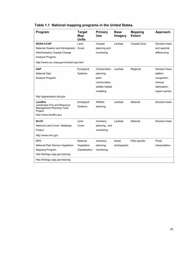
Table 1.1 National mapping programs in the United States...........................................20
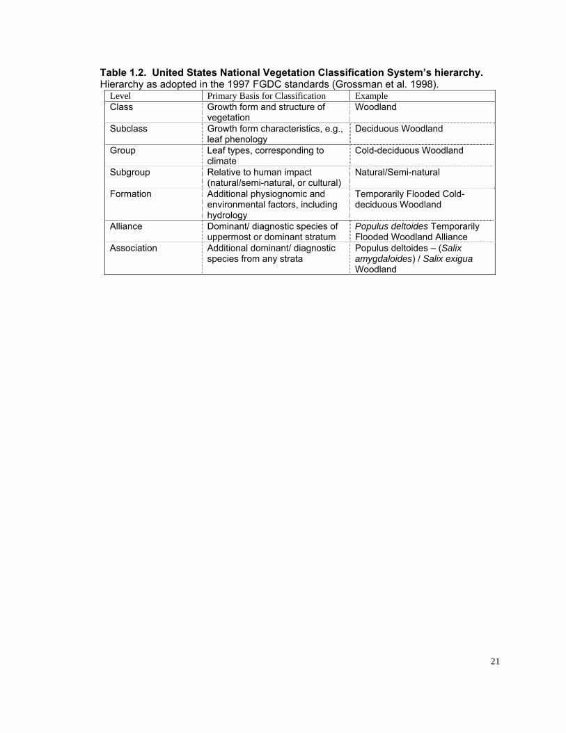
Table 1.2. United States National Vegetation Classification System’s hierarchy...........21
Table 2.1. Target vegetation map classes for the Onslow Bight, North Carolina...........67
Table 2.2. Path/Rows and Landsat TM image acquisition dates for the Onslow Bight study area. ......................................................................................................................68
Table 2.3. Wetland map classes included in Zone 58 in addition to the NLCD 2001 legend. ............................................................................................................................69
Table 2.4. Data layers available for use in decision tree modeling and for mapping. ....70
Table 2.5. Crosswalk between North Carolina Natural Heritage Program’s Natural Community and NatureServe’s Ecological Systems Classification. ................................71
Table 2.6. Ecological Systems model results.................................................................73
Table 2.7. Per class acreage and accuracy statistics for the Onslow Bight land cover. 74
Table 2.8. Accuracy assessment of the areas of disagreement in the XY and NOXY models for natural vs. managed evergreen.....................................................................75
Table 2.9. Confusion matrices for raw assessment points in each model. ....................76
Table 3.1. Thresholds used to categorize urban land cover classes from impervious surface estimates. .........................................................................................................106
Table 3.2. Major Categories of land cover change between 1992 and 2001 in the Onslow Bight. ................................................................................................................107
Table 3.3. Percent land cover change between Ecological Systems between 1992 and 2001. .............................................................................................................................108
Table 3.4. Accuracy assessment for the binary change map of the Onslow Bight. .....110
Table 3.5. Change/ no change accuracy by 1992 land cover class.............................111
Table 4.1. Eight required elements for the State Wildlife Action Plans. .......................141
Table 4.2 The six Partners in Flight species assessment factors. ................................142
Table 4.3. Categories of the model parameters used in the Southeast GAP’s habitat modeling........................................................................................................................143
Table 4.4. Definitions for the GAP Status codes...........................................................144

ix
Table 4.5. Representation of the Ecological Systems of the Onslow Bight in the Southeast ......................................................................................................................145
Table 4.6. Vertebrate species included in the North Carolina State Wildlife Action Plan but not modeled by Southeast GAP..............................................................................146
Table 4.7. Partners in Flight priority bird species of the Onslow Bight. ........................147
Table 4.8. Land cover scorecard..................................................................................148
x
LIST OF FIGURES Figure 1.1. A summary of the literature. ..........................................................................22
Figure 1.2. Relationship between the National Vegetation Classification System and the
Ecological Systems Classification. ...........................................................................23
Figure 1.2. Relationship between the National Vegetation Classification System and the
Ecological Systems Classification. ...........................................................................23
Figure 1.3a. Example of a decision tree from the Southwest Gap Analysis Project. .....24
Figure 1.3b. Thresholds from the Southwest GAP decision tree are shown as axes in
two-dimensional space. ............................................................................................25
Figure 1.4. Image objects for a small area of the Croatan National Forest....................26
Figure 1.5. Southwest GAP Regional Land Cover Map. ................................................27
Figure 2.1. Location map for the Onslow Bight Study Area with county boundaries and
Ecological Regions. ..................................................................................................77
Figure 2.2. Omission error for each Ecological System by model...................................78
Figure 2.3. Commission error for each Ecological System by model.............................79
Figure 2.4a – e. Comparison of maps of the evergreen and nonriverine Ecological
Systems....................................................................................................................80
Figure 3.1. Examples of change vectors for two sites..................................................113
Figure 3.2. Southeast Gap Analysis Project’s land cover map for the Onslow Bight, NC.
................................................................................................................................114
Figure 3.3. Flow Diagram of the preprocessing steps and identification of potential
change areas..........................................................................................................115
Figure 3.4. Flow Diagram for change detection and labeling the 1992 land cover for the
non-urban areas. ....................................................................................................116
Figure 3.5. Flow Diagram for change detection and labeling the 1992 land cover for
urban areas. ...........................................................................................................117
Figure 3.6. Date Band Combinations in the 1992 and 2001 Landsat Image Mosaics. 118
Figure 3.7. Feature space image demonstrating the characteristic “tasseled cap” pattern
for a portion of Onslow Bight study area. ...............................................................119
Figure 3.8. Land cover change areas in the Onslow Bight 1992 – 2001......................120
Figure 4.1. The Onslow Bight study area and Environmental Protection Agency Level IV
ecoregions. .............................................................................................................150
Figure 4.2. Dichotomous key used to determine the GAP Land Management Status. 151
xi
Figure 4.3 a and b. Scorecards for the State Wildlife Action Plan species on Status 1
and 2 lands (a) and on Status 3 and 4 lands (b). ...................................................152
Figure 4.4. Changes in the predicted distributions for 20 amphibian species of concern in
the North Carolina State Wildlife Plan. ...................................................................153
Figure 4.5. Changes in the predicted distributions for 58 bird species of concern in the
North Carolina Wildlife Action Plan.........................................................................154
Figure 4.6. Changes in the predicted distributions for 15 mammal species of concern in
the North Carolina State Wildlife Plan. ...................................................................155
Figure 4.7. Changes in the predicted distributions for 32 reptilian species of concern in
the North Carolina State Wildlife Plan. ...................................................................156
Figure 4.8. Score Card for Partners in Flight species of the Onslow Bight. ..................157
Figure 4.9. Changes in the predicted distributions for 38 Partners in Flight priority bird
species. ..................................................................................................................158
Figure 4.10. Species richness maps for the State Wildlife Action Plan and Partners in
Flight priorities ........................................................................................................159
Figure 4.11. Priority species hotspots for the State Wildlife Action Plan and Partners in
Flight.......................................................................................................................160
Figure 4.12. New state acquisitions relative to hot spots for SWAP and PIF priority
species richness. ....................................................................................................161
Figure 4.13 Distribution of managed land relative to predicted hotspots for the SWAP
and PIF species lists...............................................................................................162
xii
LIST OF APPENDICES
Appendix 2.1. Accuracy Assessment Confusion Matrix for the Ecological Systems Map
of the Onslow Bight ................................................................................................164
Appendix 3.1 Land cover map units for the Onslow Bight area. ...................................165
Appendix 4.1. Model parameters specific to the species distribution models in this study.
................................................................................................................................171
Appendix 4.2. North Carolina State Wildlife Action Plan species used to develop the
Onslow Bight scorecard..........................................................................................175
Appendix 4.3. Species codes, scientific and common names.......................................179

1
PREFACE
Mapping and Monitoring Plant Communities in the Coastal Plain of North Carolina: A
Basis for Conservation Planning
Alexa J. McKerrow
North Carolina State University
Decades after the international community first realized its magnitude, the decline in
global biodiversity continues. The number of imperiled species is increasing and the
acreage of degraded natural systems continues to rise. During the past twenty years
the National Gap Analysis Program (GAP) has been working to provide data and
analyses to help guide proactive conservation and management. Based on the
assumption that the most effective time to manage for a species is before it becomes
imperiled, GAP has been working with partners to develop a framework for
conservation of all vertebrate species and the natural systems upon which they
depend.
My goal in this dissertation was to explore in depth the methods and analyses that
can be employed to monitor natural systems and habitats through time. Specifically,
I wanted to test the current approaches for land cover mapping and change detection
and to use the results of that work in a conservation assessment that could be used
by a variety of natural resource management agencies.
Chapter one represents a review of the current literature with respect to vegetation
mapping in the United States. It details a variety of approaches that are being used
and includes a discussion of the national classification systems (National Vegetation
Classification System, Ecological Systems Classification) currently in use.
Chapter two details the mapping of vegetation of the Onslow Bight of NC. I used
Landsat TM satellite imagery and a combination of ancillary datasets to map the
Ecological Systems of the area. The change detection described in Chapter three
2
allowed the creation of a two date time series (1992 and 2001) for the Ecological
Systems of Onslow Bight.
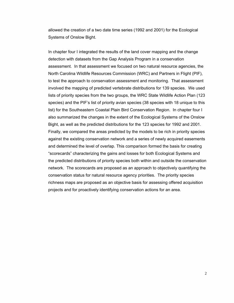
In chapter four I integrated the results of the land cover mapping and the change
detection with datasets from the Gap Analysis Program in a conservation
assessment. In that assessment we focused on two natural resource agencies, the
North Carolina Wildlife Resources Commission (WRC) and Partners in Flight (PIF),
to test the approach to conservation assessment and monitoring. That assessment
involved the mapping of predicted vertebrate distributions for 139 species. We used
lists of priority species from the two groups, the WRC State Wildlife Action Plan (123
species) and the PIF’s list of priority avian species (38 species with 18 unique to this
list) for the Southeastern Coastal Plain Bird Conservation Region. In chapter four I
also summarized the changes in the extent of the Ecological Systems of the Onslow
Bight, as well as the predicted distributions for the 123 species for 1992 and 2001.
Finally, we compared the areas predicted by the models to be rich in priority species
against the existing conservation network and a series of newly acquired easements
and determined the level of overlap. This comparison formed the basis for creating
“scorecards” characterizing the gains and losses for both Ecological Systems and
the predicted distributions of priority species both within and outside the conservation
network. The scorecards are proposed as an approach to objectively quantifying the
conservation status for natural resource agency priorities. The priority species
richness maps are proposed as an objective basis for assessing offered acquisition
projects and for proactively identifying conservation actions for an area.

3
Recent trends in remote sensing for vegetation mapping in the United States. Alexa J. McKerrow1, Thomas R. Wentworth2 and Milo Pyne3. 1 Southeast Gap Analysis Project, Department of Zoology, North Carolina State University, Raleigh, NC 27695-7617 ([email protected]); 2 Department of Plant Biology, North Carolina State University 27695-7612 ([email protected]); 3 NatureServe, 6114 Fayetteville Rd, Suite 109, Durham, NC 27713 ([email protected]). Abstract High quality land cover data is the key to an effective assessment of the status of
vegetation of the United States. Recent innovations in mapping technology are making
it possible to map vegetation over large areas with relatively high levels of thematic
detail. During the past decade the vegetation mapping discipline has seen major
advances in vegetation classification, satellite imagery, and mapping approaches. The
development of the National Vegetation Classification System and Ecological
Classification System provides a framework for map legends that are ecologically
meaningful and consistent across the country. Access to satellite imagery and synergy
between national mapping programs has greatly increased the efficiency of land cover
mapping in the U.S. Finally, methods for large area mapping (e.g., image stratification,
decision tree modeling, and pattern recognition) are providing a solid foundation for
mapping the vegetation of the country. In this review we discuss the evolution of
vegetation mapping methods during the past decade, describe some of the national
programs involved in vegetation mapping, and provide an overview of the current status
of vegetation classification systems in the U.S.
In a Nutshell
• The ability to map vegetation over large areas is the basis for effective land
management and conservation.
• The feasibility of vegetation mapping over large areas is rapidly accelerating.
• The National Vegetation Classification System and Ecological Systems
Classification are evolving to provide a much-needed framework for vegetation
mapping in the U.S.
4
• New innovations (e.g., pattern recognition, hyperspectral and hyperspatial
imagery) are currently limited to small extents, but should become practical for
large area mapping soon.
Introduction Vegetation mapping has undergone a considerable change in the last decade. In
particular, integrating the perspective gained from space has made vegetation mapping
of large areas possible. Changes in how government programs acquire and distribute
remotely sensed data, and advances in computing power and mapping techniques, are
removing some of the previously existing barriers to mapping large extents. The
application of geographic information systems (GIS) science has also rapidly expanded,
with agencies incorporating spatial data into their programs, and universities increasing
opportunities for training. As a result, researchers and land managers are increasingly
reliant on spatial data for inventory, management, and planning. Today, vegetation
mapping is done from local to global scales, and those maps inform studies on global
climate change (Freidl et al. 2003), deforestation (Skole and Tucker 1993),
desertification (Hanan et al. 1991), habitat management (Scott et al. 1993, Scott and
Jennings 1998, Lowry et al. 2005) and wildfire planning (Falkowski et al. 2005) (Figure
1.1). Recent innovations in data availability and mapping methodology have allowed the
development of a global land cover map (Belward et al. 1999), a standard protocol for
rapidly mapping general land cover of the U.S. (Homer et al. 2004), detailed large scale
vegetation maps for some National Parks and Wildlife Refuges (Welch et al. 2002),
vegetation maps for large regions (Lowry et al. 2005), and land cover change maps for
the coastal regions (NOAA CCAP 2006). Table 1.1 provides a summary of programs
currently involved in national mapping efforts in the U.S.
Just as important as the advances in mapping techniques, the standard vegetation
classification systems that have been developed over the last decade are vastly
improving the utility of the maps being developed. The National Vegetation Classification
System (NVC; Grossman et al. 1998) was the first attempt at a nationally consistent
system for all terrestrial vegetation. That classification and the Ecological Systems
Classification (Comer et al. 2003) are the most broadly applied classification systems in
vegetation mapping in the United States today.
5
The goal of this review is to summarize the recent developments in mapping techniques
and vegetation classification specific to current mapping programs in the United States
and to discuss some of the common tradeoffs (e.g., among extent, spatial resolution,
and thematic resolution) to be considered when planning or evaluating a mapping
project. In this review we are aiming for two general audiences, the ecologist
considering a vegetation mapping project, and land managers who need to evaluate the
land cover and vegetation maps they encounter in the course of their careers.
Target Map Classes
The first step in a successful mapping project is the identification of the target map
classes. The intended use of the final map and the limitations of the data being used to
create it will determine and constrain the number and definition of these classes.
A priori vs. derived map classes There are two general methods for determining the vegetation classes: selecting from an
a priori classification scheme or deriving the classes from a study area-specific dataset.
In many maps, photo-interpretation is used for gathering data to train image
classification or for directly mapping land cover. In those cases, the legend is
determined by the ability to distinguish the target classes consistently in the
photography. In this case, the photo-interpretation key represents the a priori
classification scheme. Other examples of a priori classification systems are the detailed
vegetation classification systems (Daubenmire and Daubenmire 1968, Schafale and
Weakley 1990) for areas where plant community ecologists have focused their work.
Classification systems vary depending on their geographic extent and the resource-
specific objectives of the classification. It was not until 1998 that the U.S. had its first
national-level classification of vegetation, the National Vegetation Classification System
(NVCS; Grossman et al. 1998). Because of the importance of this a priori classification
to national programs we discuss recent developments in detail below.
An alternative to a priori map classes is the use of detailed plot sampling and
quantitative analysis of species composition to derive a classification scheme. The latter
most often rely on cluster analysis and ordination techniques to determine the
6
appropriate number and identity of vegetation classes in a study area. Each derived
classification is a reflection of the dataset used in its development; as the datasets
become richer with continued sampling, the spatial extent and thematic resolution of the
derived classifications increase accordingly (Peet and Allard 1993, Reid et al. 1995,
Newell et al. 1997, and Simon et al. 2005).
National vegetation classification systems As the technology for mapping vegetation over large areas matured in the early 1990s,
the lack of a standard classification system became increasingly problematic. The
NVCS was developed as a hierarchical classification scheme in an attempt to address
the need for a classification scheme that was national in scope and thorough (Jennings
1997). It was developed as a hierarchical classification scheme similar in concept to that
used in the United Nations Educational, Scientific, and Cultural Organization
international classification of vegetation (UNESCO 1973). The NVCS hierarchy has 7
levels; in the upper five levels it includes physiognomic, structural, growth-form,
phenological, and environmental information (Table 1.2). The lowest two levels
incorporate species composition information. Dominant and/or indicator species of the
uppermost or dominant layer (e.g., the canopy in a forest) determine the alliance
classification, and additional subcanopy and/or ground layer species help define the
associations. Currently, the Vegetation Subcommittee of the Federal Geographic Data
Committee is drafting a revision of the NVCS standard (ESA Panel on Vegetation
Classification 2004). If adopted, that revised standard may alter the structure of the
hierarchy, while encouraging collaboration toward the evolution of the detailed content of
the NVCS through a peer review process.
Since 1998 many programs have attempted to implement mapping of the NVCS at
various levels of the hierarchy. The most successful of these has been the National
Park Service (NPS) Mapping Program (http://biology.usgs.gov/npsveg/). NPS has been
systematically mapping many of the national parks at the association level, the finest
level of the NVCS. The Park Service has been able to achieve a high thematic
resolution with extensive field work and manual interpretation of large scale aerial
photography (TNC and ESRI 1994).
7
In the mid-1990s the USGS Biological Resources Division‘s Gap Analysis Program
(GAP) selected the Alliance level of the NVCS as the basis for a state-by-state set of
target map classes, but reliable (consistent and accurate) representation of these
classes could not be achieved. This was due to an incompatibility between the spatial
scale of the vegetation types on the ground and the scale of the available imagery and
ancillary data. Scaling back to the Formation (the next highest level in the hierarchy)
would have meant a loss of important ecological context. In the short-term this led to a
shift in the target map legend for the individual state GAP projects (Pearlstine et al.
1998) and a broader call for an ecologically meaningful and “mappable” classification
system. With support of groups like The Nature Conservancy and the National Gap
Analysis Program, NatureServe ecologists were able to build on the extensive research
and data of the NVCS to develop the first draft of this new classification, the Ecological
Systems of the United States (Comer et al. 2003). Each system is intended to represent
a group of associations tied together by landscape level ecological processes. It is
important to note that this classification is not hierarchical and, while it is informed by the
NVCS, it is a parallel system. The only direct link between the two classifications is at
the finest level of the NVCS, the association (Figure 1.2). Because ecological processes
(flooding, fire, wind) are central to the definition of the Ecological Systems, ancillary data
are often necessary for mapping where spectral data alone would be insufficient.
Trends in satellite-based mapping
In their book ”Vegetation Mapping”, Kuchler and Zonneveld (1988) provided the first
broad introduction to the field of satellite-based mapping. In 1994, Zhu and Evans
published a forest map for the United States based on 1x1km Advanced Very High
Resolution Radiometer (AVHRR) imagery, and, in 1997, Friedl and Brodley tested the
use of decision tree modeling for satellite based mapping. By the mid-1990’s, the
National Land Cover Dataset (NLCD) and GAP state projects were making important
advances in large area mapping. Below we present a summary of the traditional
methods used in remote sensing and a discussion of recent innovations, including the
use of multi-temporal imagery and the integration of ancillary spatial data and remote
sensing.

8
Landsat imagery and vegetation mapping Currently, Landsat Thematic Mapper (TM) and Enhanced Thematic Mapper (ETM)
sensors dominate the field with respect to large area vegetation mapping in the United
States. The National Gap Analysis Program, NOAA Coastal Change Analysis Program
(CCAP), and the Landfire Project all use Landsat imagery as the base for detailed
vegetation mapping for large regions of the U.S. Landsat TM and ETM sensors acquire
data for 6 and 7 spectral bands, respectively, at a spatial resolution of 30x30 m. Each of
the Landsat sensors acquires data on a 16 day return cycle, although cloud cover and
seasonal variability limit the number of those acquired images that might be suitable for
mapping. The broad application and reliance on Landsat imagery for vegetation
mapping in the U.S. is reflected in the following discussion. For a treatment of the use of
Landsat in broader ecological applications see Cohen and Goward (2004).
Manual interpretation vs. automated computer mapping The general trend in satellite-based land cover mapping is from manual methods toward
an increased reliance on computer assisted and automated mapping methods. Early
uses of satellite imagery as the base layer for mapping involved manual delineating and
labeling of polygons. For example, the first generation vegetation map for the
Washington State GAP project was developed through visual interpretation of Landsat
TM imagery and field visits to guide the labeling of polygons (Grue 1997). Similarly, in
their assessment of coastal sage scrub, Davis et al. (1994) used Landsat TM to
delineate patterns, combined with field reconnaissance, interpretation of aerial
photographs, and reference to historic maps in the labeling stage. The success and
feasibility of manually delineating patterns in vegetation depend on the skill of the
interpreter, the quality of the reference data, and the complexity of the vegetation being
mapped.
The two traditional automated computer mapping approaches for image classification
are unsupervised and supervised classification (Jensen 2004). In an unsupervised
classification, each pixel in the image is assigned membership to an image cluster based
on the statistical similarity of the pixel to a cluster. Similarity is determined by calculating
the mean of all of the pixels currently assigned to a cluster for each band in the imagery.
Clustering is an iterative process where pixels are sorted into a predetermined number
9
of bins (clusters) based on the mean of the pixels currently assigned to each cluster. In
each iteration, the membership of each pixel is re-evaluated based on the means of the
clusters. Labeling of the imagery to generate a map is then done using training data to
identify the most likely vegetation type for each cluster. In this case, the clusters
represent groupings of the data that must then be interpreted and labeled relative to the
map legend.
In contrast to an unsupervised method, which requires that data for labeling classes be
gathered after the membership of pixels has been assigned, a supervised method
utilizes a training dataset, derived in advance and used to train the classification. The
goal in developing the training dataset is to select homogeneous training areas that
represent the range of variability for each target map class. In the classification stage,
each pixel in the study area is compared to the groups of pixels in each area of the
training dataset and the pixels are assigned a map class if they are statistically similar to
one of the training signatures. With a small study site or a generalized map legend,
either a supervised or unsupervised approach is likely to be adequate for mapping
vegetation. The accuracy of an unsupervised classification will depend on the target
map legend, input imagery, and the analyst’s ability to discriminate the land cover
classes in the imagery. Supervised classification is most sensitive to the quality of the
training data and the algorithm (e.g., maximum likelihood, minimum distance) used to
label the land cover classes.
Multi-temporal imagery As access to imagery and processing power increased, references to the use of multi-
temporal imagery for mapping became more prevalent in the literature (Egbert et al.,
1995; Wolter et al. 1995). A current example of the use of multi-temporal imagery for
land cover mapping is the National Land Cover Dataset (NLCD 2001; Homer et al.
2004). That database includes the creation of three seasonal image mosaics (spring,
leaf on, and leaf off) for each mapping zone in the U.S. (Yang et al. 2001). Such
mosaics are also being used for the Gap Analysis Program, NOAA’s Coastal Change
Analysis Program (CCAP), and the Landfire Project, as well as in mapping for the NLCD
2001. For each of those efforts, the temporal variation is being used indirectly to assist
10
in refining the land cover classifications and treat each date of imagery as an
independent source of information.
Other approaches use information from the multi-temporal images directly, either by
incorporating information about the change vectors (Lunetta et al. 2001) or by selecting
which image(s) to use in classifying specific vegetation types. For example, Townsend
(1997) used a hierarchical approach in which coarse vegetation types were mapped and
then refined by developing unique combinations of multi-temporal image bands and
band ratios for refinement of the detailed wetland classes. Wolter et al. (1995) used a
similar hierarchical approach with specific band combinations from various image dates
to map forest types in northwestern Wisconsin. Incorporating multi-temporal imagery
increased the thematic resolution of maps from both Landsat (Mickelson et al. 1998,
Wolter et al. 1995, Slaymaker et al. 1996) and Advanced Very High Resolution
Radiometer imagery (Stoms et al. 1998, Zhu and Evans 1994).
Integrating ancillary data and remote sensing Methods for integrating ancillary spatial data and remote sensing can be generally
categorized as image stratification (either pre- or post-classification; Edwards et al.
1995, Gao et al. 2004); preponderance of evidence decision rules (Sader et al. 1995,
Lunetta et al. 2001, Felicisimo et al. 2002); generalized linear modeling (Moisen and
Edwards 1999); gradient nearest neighbor (Ohmann and Gregory 2002); or evidential
reasoning approaches, including decision tree modeling (Duguay and Peddle 1996,
Homer et al. 2004).
Image stratification by ecological region In the Utah and Southwest GAP Projects (Edwards et al. 1995; Lowry et al. 2005),
ecological regions were used to stratify the study area. In each case the assumption
was that variability with respect to the target map classes would be lower within regions
than among them. Similar logic was used in the development of the mapping zones for
the NLCD 2001 (Homer and Gallant 2001). In that effort, the mapping zones were
delineated based on five criteria - size, physiography, land cover patterns, spectral
patterns, and the placement of the map zone edges that would later need to be
mosaicked with adjoining zones. Large area mapping involved mapping across many
11
satellite scenes. If each scene is mapped individually, adequate training data for each
land cover class being mapped must be located within each of those scenes. If
however, the imagery is mosaicked and then divided based on ecoregion, the mapper
may be able to map the same classes with a lower number of training points overall.
Another potential advantage is the reduction in edge matching, assuming the ecoregion
boundaries do represent transition lines for the classes being mapped. The potential
disadvantage is increased spectral variability within a region if the satellite scenes
mosaicked to create a region have high variability in phenological or atmospheric
conditions (Homer et al. 1997).
Preponderance of evidence decision rules Several projects have found they could improve the accuracy of their vegetation
mapping by incorporating preponderance of evidence decision rules, also known as
weighting criteria. A decision rule can be based on expert knowledge or can be derived
from the data. For example, if floodplain forests only occur within 100 meters of a river,
a rule can be established that floodplains can only be mapped within that distance.
Similarly, if 95% of the training sites for floodplain forest occur within 100 meters of the
river, a probability of 95% can be applied to pixels within 100 m of the river and a 5%
probability for pixels at greater distances. Incorporating variables such as elevation,
terrain type, and proximity to rivers improved the vegetation map for a site in the Arctic
National Wildlife Refuge (Joria and Jorgenson 1996). In that study, the application of
GIS-based decision rules to an unsupervised classification produced a better vegetation
map than either the unsupervised classification alone, or a supervised classification
based on the same training data. Similarly, the Utah GAP Project adopted a two-phase
mapping approach in order to improve its vegetation map (Edwards et al. 1995).
Summary statistics for the clusters from the unsupervised classification were used to
determine weighting criteria used in ancillary modeling within each ecological region of
the state. Edwards et al. (1995) found that the majority of cover classes (31 of 36) were
improved with the use of this ancillary modeling.
Generalized linear modeling An early example of using generalized linear modeling to integrate satellite imagery and
ancillary spatial data for mapping vegetation is the study of Glacier National Park (Brown
12
1994). Generalized linear modeling, like traditional linear regression, relies on least
squares criteria to model the response variable from the predictor variables. In this
study, four vegetation types (open canopy forest, closed canopy forest, meadow, and
unvegetated) were modeled from insolation potential, snow accumulation potential, and
soil moisture potential. Moisen and Edwards (1999) also used generalized linear
modeling to integrate topography, spatial coordinates, and spectral data with traditional
forest inventory data for northern Utah, and they were able to improve the precision of
forest timber volume estimates over methods based on the plot data alone.
Gradient nearest neighbor Ohmann and Gregory (2002) used gradient nearest neighbor to successfully map forest
structure and physiognomy for Coastal Oregon. This method translates the results of
traditional direct gradient analysis (Gauch 1982) into a spatial framework by assigning
map labels based on nearest neighbor imputation. In Ohmann and Gregory (2002),
Landsat TM spectral bands and derivatives were first integrated with ownership,
topographic, geologic, and climatic data derivatives and then analyzed using canonical
correspondence analysis to model forest types. The map was then created by assigning
each pixel in the study site to the class of its nearest neighbor (minimum Euclidean
distance) in gradient space. While Gradient Nearest Neighbor has been successfully
applied to mapping structure and physiognomy, it had not been previously used to map
vegetation type. Currently the approach is being tested with respect to mapping
Ecological Systems in the Northwestern U.S.
Decision tree modeling Decision tree modeling is a supervised classification method that has been broadly
applied in the social and medical sciences for decades. It was not until the 1990s that
the potential for use in land cover applications became apparent (Michaelson et al. 1994,
Duguay and Peddle 1996). Decision trees rely on recursive partitioning of the training
dataset to create a hierarchical tree in which a series of nodes represent a binary split of
the dataset into branches. The method for splitting the data depends on whether the
response variable is categorical (discriminant analysis or logistic regression) or
continuous (multiple regression). In keeping with the tree theme, the terminal nodes
where the map classes are assigned are called leaves (Figures 1.3a and b).
13
Friedl and Brodley (1997) examined the application of the decision tree process to land
cover mapping at three scales (AVHRR at 1 x 1 o; AVHRR at 1x1 km; and Landsat TM at
30x30 m) and found that, in each case, decision trees performed better than either the
linear discriminant functions or the more traditional supervised classification approach
(e.g., maximum likelihood classification).
The adoption of the decision tree classification as a central component of the NLCD
2001 protocol (Homer et al. 2004) means that the approach is being applied throughout
the U.S. for land cover mapping. The database includes three components - general
land cover (NLCD 2001), canopy closure, and impervious surface estimations.
Regression tree modeling is used to generate the estimates of canopy closure, and
impervious surface (Yang et al. 2003, Homer et al. 2004) and decision tree modeling is
used in the development of the 23-class land cover layer. The first large area mapping
effort to incorporate decision tree modeling for mapping vegetation types in the U.S. was
the Southwest GAP Project (Lowry et al. 2005, see Case Study).
Pattern recognition An additional innovation in mapping is the use of pattern recognition, in which texture or
context information for individual pixels is used in combination with the spectral
information to create image objects (Figure 1.4). In their discussion, “What’s the matter
with pixels? Some recent developments in interfacing remote sensing and GIS”,
Blaschke and Strobl (2001) provide a thoughtful summary of the need to pay attention to
pattern in land cover mapping. They proposed location and context as “new paradigms”
in remote sensing. Some of their concepts can be related back to work by Ryherd and
Woodcock (1996), who showed the importance of incorporating texture information into
image segmentation. In that study, forests of various canopy densities and mixtures of
tree canopy sizes were simulated to test the accuracy of forest pattern delineation with
and without texture as an input. In southern Montana, Fisher et al. (2002) tested the
application of two pattern recognition approaches to mapping. They were able to map
27 cover classes, using supervised classification based on image objects, with overall
accuracies greater than 70%. In the same study they found they were able to map five
sagebrush and greasewood species with over 90% accuracy using the same methods.
14
The use of pattern recognition in large area vegetation mapping is limited (Fisher et al.
2002, Chapter 2 and 3 this volume). Current applications tend to involve highly
structured land cover or land use classes (e.g., roads, buildings) with an emphasis on
high resolution imagery (e.g., IKONOS, digital orthophotography; Elmqvist and Khatir
2007). The application of pattern recognition in mapping based on lower resolution
imagery for natural resource applications is expanding (Lucas et al. 2007, Fisher et al.
2002, Chapter 2 and 3 this volume).
Future Trends We can expect that, over the next few years, decision tree modeling will continue to be
the dominant method for large area vegetation mapping. At the same time, it is likely
that the application of pattern recognition and higher resolution satellite imagery
(hyperspectral and hyperspatial) will become increasingly common as barriers to their
use (limited access, high cost, and limited processing capabilities) are removed. The
continued evolution of the NVCS, including the adoption of a new hierarchy structure
and continued inventory work, will make use of that classification for large area mapping
practical.
Acknowledgements We thank John Lowry of the Remote Sensing/GIS laboratory at Utah State for supplying
sample data from the Southwest Gap Analysis Project, U.S. Geological Survey for the
map of Southwest GAP land cover, and K. Kostelnik, W. Wall, W. Hoffman, and R.
Marchin for their comments on earlier drafts of this review.
References Belward, A. S., J. E. Estes, and K. D. Kline. 1999. The IGBP-DIS Global 1-Km land-
cover data set DISCovery: A project overview. Photogramm Eng Rem S 65:1013-1020.
Blaschke, T. and J. Strobl. 2001. What’s wrong with pixels? Some recent developments interfacing remote sensing and GIS. GIS—Zeitschrift für Geoinformationssysteme 6:12–17.
Brown, D. G. 1994. Predicting vegetation types at treeline using topography and biophysical disturbance variables. J Vege Sci 5:641-656.
15
Cohen, W. B. and S. N. Goward. 2004. Landsat’s role in ecological applications in remote sensing. BioSci 54:535-545.
Comer, P., D. Faber-Langendoen, R. Evans, S. Gawler, C. Josse, G. Kittel, S. Menard, M. Pyne, M. Reid, K. Schulz, K. Snow, and J. Teague. 2003. Ecological Systems of the United States: A working classification of U.S. terrestrial systems NatureServe, Arlington, VA.
Daubenmire, R. and J. B. Daubenmire. 1968. Forest vegetation of eastern Washington and northern Idaho. Technical Bulletin 60. Washington Agricultural Experiment Station, College of Agriculture, Washington State University, Pullman, 104 pp.
Davis, F. W., P. A. Stine, and D. M. Stoms. 1994. Distribution and conservation status of coastal sage scrub in southwestern California. J Vege Sci 5:743-756.
Ecological Society of America Vegetation Panel. 2004. Vision statement and report on panel activities. http://www.esa.org/vegweb/#panel. Viewed 12/1/07.
Edwards, T.C., Jr., C. G. Homer, S. D. Bassett, A. Falconer, R. D. Ramsey, and D. W. Wight. 1995. Utah Gap Analysis: an environmental information system. Technical Report 95-1, Utah Cooperative Fish and Wildlife Research Unit, Utah State University, Logan, Utah. 1189pp + 2 CD-ROMs.
Egbert, S. L., K.P. Price, M. D. Nellis, and R. Lee. 1995. Developing a land cover modeling protocol for the high plains using multi-seasonal thematic mapper imagery. Proceedings of the Annual Convention and Exposition. American Congress on Surveying and Mapping / American Society for Photogramm Eng Rem S 3:836-845.
Elmqvist, B. and A. R. Khatir. 2007. Journal of Arid Environments. The possibilities of bush fallows with change roles of agriculture – An analysis combining remote sensing and interview data from Sudanese drylands. J. of Arid Envir 70:329-343.
Duguay, C. R. and D. R. Peddle. 1996. Comparison of Evidential Reasoning and Neural Network Approaches in a Multi-Source Classification of Alpine Tundra Vegetation. Can J of Rem S 22:422-403.
Falkowski, M. J., P. E. Gessler, P. Morgan, A.T. Hudak, M.S. Alistair. 2005. Characterizing and mapping forest fire fuels using ASTER imagery and gradient modeling. For Ecol and Manage 217:129-146.

16
Fisher, C., W. Gustafson, and R. Redmond. 2002. Mapping Sagebrush/Grasslands from Landsat TM-7 Imagery: A Comparison of Methods. Report to the US DOI - Bureau of Land Management. Billings, MT 1-21. http://sagemap.wr.usgs.gov/Docs/BLM_sagecompare.pdf. Viewed 12/1/07.
Friedl, M. A. and C. E. Brodley. 1997. Decision tree classification of land cover from remotely sensed data. Rem S Envir 61:399-409.
Gao, J., H, Chen, and Y. Zha. 2004. Knowledge-Based Approaches to Accurate Mapping of Mangroves from Satellite Data. Photogramm Eng Rem S 17:1241-1249.
Gauch, H. G., Jr. 1982. Multivariate Analysis and Community Structure. Cambridge University Press, Cambridge.
Grossman, D. H., D. Faber-Langendoen, A. S. Weakley, M. Anderson, P. Bourgeron, R. Crawford, K. Goodin, S. Landaal, K. Metzler, K. D. Patterson, M. Pyne, M. Reid, and L. Sneddon. 1998. International classification of ecological communities: Terrestrial vegetation of the United States. Volume I. The National Vegetation Classification System: Development, status, and applications. The Nature Conservancy, Arlington, Virginia. 126 p.
Grue, C.E., K. M. Cassidy, and K. M. Dvornich. 1997. Washington State Gap Analysis Project Final Report. Submitted to USGS. Biological Resources Division. National Gap Analysis Program. Five volume cd-rom set.
Hanan, N. P., Y. Prevost, A. Diouf, and O. Diallo. 1991. Assessment of desertification around deep wells in the sahel using satellite imagery. J Applied Ecol 28:173-186.
Homer, C. G. and A. Gallant. 2001. Partitioning the Conterminous United States into Mapping Zones for Landsat TM Land Cover Mapping, USGS Draft White Paper, 2001. 7 p.
Homer, C., C. Huang, L. Yang, B. Wylie, and M. Coan. 2004. Development of a 2001 National Landcover Database for the United States. Photogramm Eng Rem S 70:829-840.
Homer, C. G., R. D. Ramsey, T. C. Edwards, Jr. and Alan Falconer. 1997. Landscape Cover-Type Modeling Using a Multi-Scene Thematic Mapper Mosaic. Photogramm Eng Rem S 63:59-67.
17
Jensen, J. R. 2004. Introductory Digital Image Processing. 3rd Edition, 2004. Prentice Hall. 526 p.
Jennings, M. D. 1997. Progressing toward a standardized classification of vegetation for the U.S. U.S.G.S. Biological Resources Division. National Gap Analysis Program Bulletin 6:16-19.
Joria, P. E. and J. E. Jorgenson. 1996. Comparison of three methods for mapping tundra with Landsat digital Data. Photogramm Eng Rem S 62:163-169.
Lowry, J. H. Jr., R. D. Ramsey, K. Boykin, D. Bradford, P. Comer, S. Falzarano, W. Kepner, J. Kirby, L. Langs, J. Prior-Magee, G. Manis, L. O’Brien, K. Pohs, W. Rieth, T. Sajwaj, S. Schrader, K. A. Thomas, D. Schrupp, K. Schulz, B. Thompson, C. Wallace, C. Velasquez, E. Waller, and B. Wolk. 2005. The Southwest Regional Gap Analysis Project Final Report on Land Cover Mapping Methods. Report to the U.S.G.S Biological Resources Division. National Gap Analysis Program 1-50. http://ftp.nr.usu.edu/swgap/swregap_landcover_report.pdf. Viewed 10/15/07.
Lucas, R., A. Rowlands, A. Brown, S. Keyworth, and P. Bunting. 2007. Rule-based classification of multi-temporal satellite imagery for habitat and agricultural land cover mapping. J of Photogramm Rem S 62:165-185.
Lunetta, R., J. Ediriwickrema, J. Iames, D. Johnson, J. Lyon, A. McKerrow and A. Pilant. 2001. A Quantitative Assessment of a Combined Spectral and GIS Rule-Based Land-Cover Classification of the Neuse River Basin, North Carolina, USA. Photogramm Eng Rem S 69:299-310.
Mickelson, J. G., D. L. Civco, J. A. Silander, Jr. 1998. Delineating Forest Canopy Species in the Northeastern United States Using Multi-temporal TM Imagery. Photogramm Eng Rem S 64:891-904.
Moisen, G. G. and T. C. Edwards, Jr. 1999. Use of generalized linear models and digital data in a forest inventory of northern Utah. J of Agricul, Biol, and Environ Stat 4:372-390.
National Oceanographic and Atmospheric Administration. Coastal Services Center. 1995-present. The Coastal Change Analysis Program (CCAP). Charleston, SC: NOAA Coastal Services Center. http://www.csc.noaa.gov/crs/lca/ccap.html. Viewed 12/1/07.
18
Newell, C. L., R. K. Peet, and J. C. Harrod. 1997. Vegetation of Joyce Kilmer-Slickrock Wilderness, North Carolina. University of North Carolina – Chapel Hill, Curriculum in Ecology and Department of Biology. 282 pages.
Ohmann, J. L. and M. J. Gregory. 2002. Predictive mapping of forest composition and structure with direct gradient analysis and nearest neighbor imputation in coastal Oregon, U.S.A. Can J For Res 32:725-741.
Pearlstine, L, A. McKerrow, M. Pyne, S. Williams, and S. McNulty. 1998. Compositional groups and ecological complexes: a methodological approach to realistic GAP mapping. Gap Analysis Bulletin No. 7. National Gap Analysis Program, Moscow, Idaho, USA. http://www.gap.uidaho.edu/Bulletins/7/CGECAMABVM.htm. Viewed 12/1/07.
Peet, R.K. and D.J. Allard. 1993. Longleaf pine vegetation of the Southern Atlantic and Eastern Gulf Coast regions: A preliminary classification. Proc Tall Timbers Fire Ecol Conf 18:45-81.
Reid, M., P. Bourgeron, H. Humphries, and M. Jensen. 1995. Documentation of the modeling of potential vegetation at three spatial scales using biophysical settings in the Columbia River Basin Assessment Area. Report to the U.S. Forest Service. 195 pp.
Ryherd, S. and C.E. Woodcock, 1996. Combining spectral and texture data in the segmentation of remotely sensed images. Photogramm Eng Rem S 62:181-194.
Sader, S.A., D. Ahl, and L. Wen-Shu. 1995. Accuracy of Landsat-TM and GIS Rule-Based Methods for Forest Wetland Classification in Maine. Rem S Environ 53:133-144.
Scott, J.M., F. Davis, B. Csuti, R. Noss, B. Butterfield, C. Groves, H. Anderson, S. Caicco, F. D'Erchia, T.C. Edwards, Jr., J. Ulliman, and R.G. Wright. 1993. Gap Analysis: A geographic approach to the protection of biological diversity. Wildlife Monographs. 123: 1-41.
Scott, J. M. and M. D. Jennings 1998. Large-Area mapping of biodiversity. Annals of the Missouri Botanical Garden: 85:34-47.
Simon, S.S., T.K. Collins, G.L. Kauffman, W.H. McNab, and C.C. Ulrey. 2006. Ecological zones in the Southern Appalachians: first approximation. Research Paper SRS-41. U.S. Department of Agriculture, Forest Service, Southern Research Station. Asheville, North Carolina. 41 p.
19
Skole, D. and C. Tucker. 1993. Tropical deforestation and habitat fragmentation in the Amazon: Satellite data from 1978 to 1988. Science 260: 1905-09.
Slaymaker, D. M., K. M. L. Jones, C. R. Griffin, J. T. Finn. 1996. Mapping deciduous forests in New England using aerial videography and multi-temporal Landsat TM imagery. In Gap Analysis: A landscape approach to biodiversity planning. Editors J. M. Scott, T. H. Tear, and F. W. Davis. ASPRS. Bethesda, Maryland. 87-102.
Stoms, D. M., M. J. Bueno, F. W. Davis, K. M. Cassidy, K. L. Driese, and J. S. Kagan. 1998. Map-guided classification of regional land cover with multi-temporal AVHRR data. Photogramm Eng Rem S 64:831-838.
The Nature Conservancy and Environmental Systems Research Institute, Inc. 1994. Final Draft: Field Methods for Vegetation Mapping. Prepared for the U.S. Department of Interior, National Biological Survey and National Park Service. (http://biology.usgs.gov/npsveg/fieldmethods/indexdoc.html; Viewed 12/18/06.
Welch, R., M. Madden, and T. Jordan. 2002. Photogrammetric and GIS techniques for the development of vegetation databases of mountainous areas: Great Smoky Mountain National Park. Photogramm Eng Rem S 57:53-68.
Wolter, P. T., D. J. Miadenoff, G. E. Host, and T. R. Crow. 1995. Improved Forest Classification in the Northern Lakes States Using Multi-Temporal Landsat Imagery. Photogramm Eng Rem S 61:1129-1143.
Yang, L., C. Homer, K. Hegge, C. Huang, B. Wylie, and B. Reed. 2001. A Landsat 7 Scene Selection Strategy for a National Land Cover Database. Proceedings of the IEEE 2001 International Geoscience and Remote Sensing Symposium, Sydney, Australia. http://search.yahoo.com/search?fr=slv1-&p=A+Landsat+7+Scene+Selection+Strategy+for+a+National+Land+Cover+Database Viewed 12/1/07.
Zhu, Z. and D. L. Evans. 1994. U.S. forest types and predicted percent forest cover from AVHRR data. Photogramm Eng Rem S 60:525-531.
20
Table 1.1 National mapping programs in the United States.
Program Target Map Units
Primary Use
Base Imagery
Mapping Extent
Approach
NOAA-CCAP National Oceanic and Atmospheric
Administration Coastal Change
Analysis Program
Land
Cover
Coastal
planning and
monitoring
Landsat Coastal Zone Decision trees
and spectral
differencing
http://www.csc.noaa.gov/crs/lca/ccap.html
GAP National Gap
Analysis Program
Ecological
Systems
Conservation
planning,
plant
communities,
wildlife habitat
modeling
Landsat Regional Decision trees,
pattern
recognition,
manual
delineation,
expert opinion
http://gapanalysis.nbii.gov
Landfire Landscape Fire and Resource Management Planning Tools Project
Ecological
Systems
Wildfire
planning
Landsat National
Decision trees
http://www.landfire.gov
NLCD National Land Cover Database
Project
Land
Cover
Inventory,
planning, and
monitoring
Landsat National Decision trees
http://www.mrlc.gov
NPS
National Park Service Vegetation
Mapping Program
http://biology.usgs.gov/npsveg
National
Vegetation
Classification
Inventory,
planning,
monitoring.
Aerial
photographs
Park specific Photo
interpretation
http://biology.usgs.gov/npsveg
21
Table 1.2. United States National Vegetation Classification System’s hierarchy. Hierarchy as adopted in the 1997 FGDC standards (Grossman et al. 1998).
Level Primary Basis for Classification Example Class Growth form and structure of
vegetation Woodland
Subclass Growth form characteristics, e.g., leaf phenology
Deciduous Woodland
Group Leaf types, corresponding to climate
Cold-deciduous Woodland
Subgroup Relative to human impact (natural/semi-natural, or cultural)
Natural/Semi-natural
Formation Additional physiognomic and environmental factors, including hydrology
Temporarily Flooded Cold-deciduous Woodland
Alliance Dominant/ diagnostic species of uppermost or dominant stratum
Populus deltoides Temporarily Flooded Woodland Alliance
Association Additional dominant/ diagnostic species from any strata
Populus deltoides – (Salix amygdaloides) / Salix exigua Woodland
21
0
459
30
42
3
420
37
225
21
2
0
82
6
1
6
33
7
17
11
0 100 200 300 400 500
97-06
Wildfire 87-96
97-06
Habitat 87-96
97-06
Desertification 87-96
97-06
Deforestation 87-96
97-06
Climate Change 87-96 Vegetation MapLand Cover
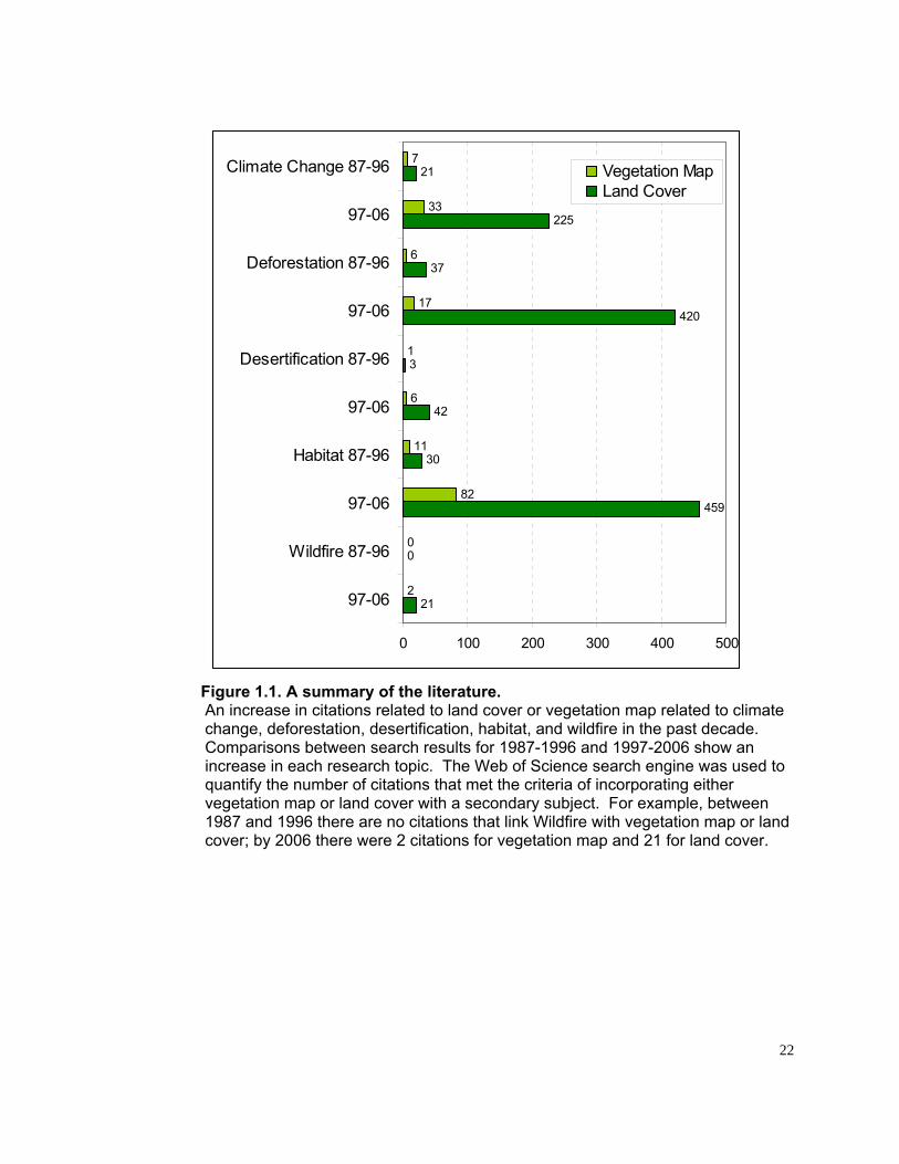
Figure 1.1. A summary of the literature. An increase in citations related to land cover or vegetation map related to climate change, deforestation, desertification, habitat, and wildfire in the past decade. Comparisons between search results for 1987-1996 and 1997-2006 show an increase in each research topic. The Web of Science search engine was used to quantify the number of citations that met the criteria of incorporating either vegetation map or land cover with a secondary subject. For example, between 1987 and 1996 there are no citations that link Wildfire with vegetation map or land cover; by 2006 there were 2 citations for vegetation map and 21 for land cover.
22
23
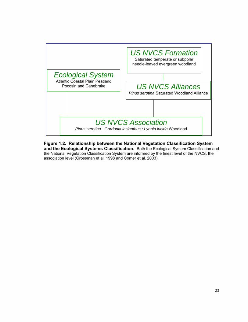
Figure 1.2. Relationship between the National Vegetation Classification System and the Ecological Systems Classification. Both the Ecological System Classification and the National Vegetation Classification System are informed by the finest level of the NVCS, the association level (Grossman et al. 1998 and Comer et al. 2003).
US NVCS Association Pinus serotina - Gordonia lasianthus / Lyonia lucida Woodland
US NVCS Alliances Pinus serotina Saturated Woodland Alliance
US NVCS Formation Saturated temperate or subpolar
needle-leaved evergreen woodland
Ecological System Atlantic Coastal Plain Peatland
Pocosin and Canebrake
24
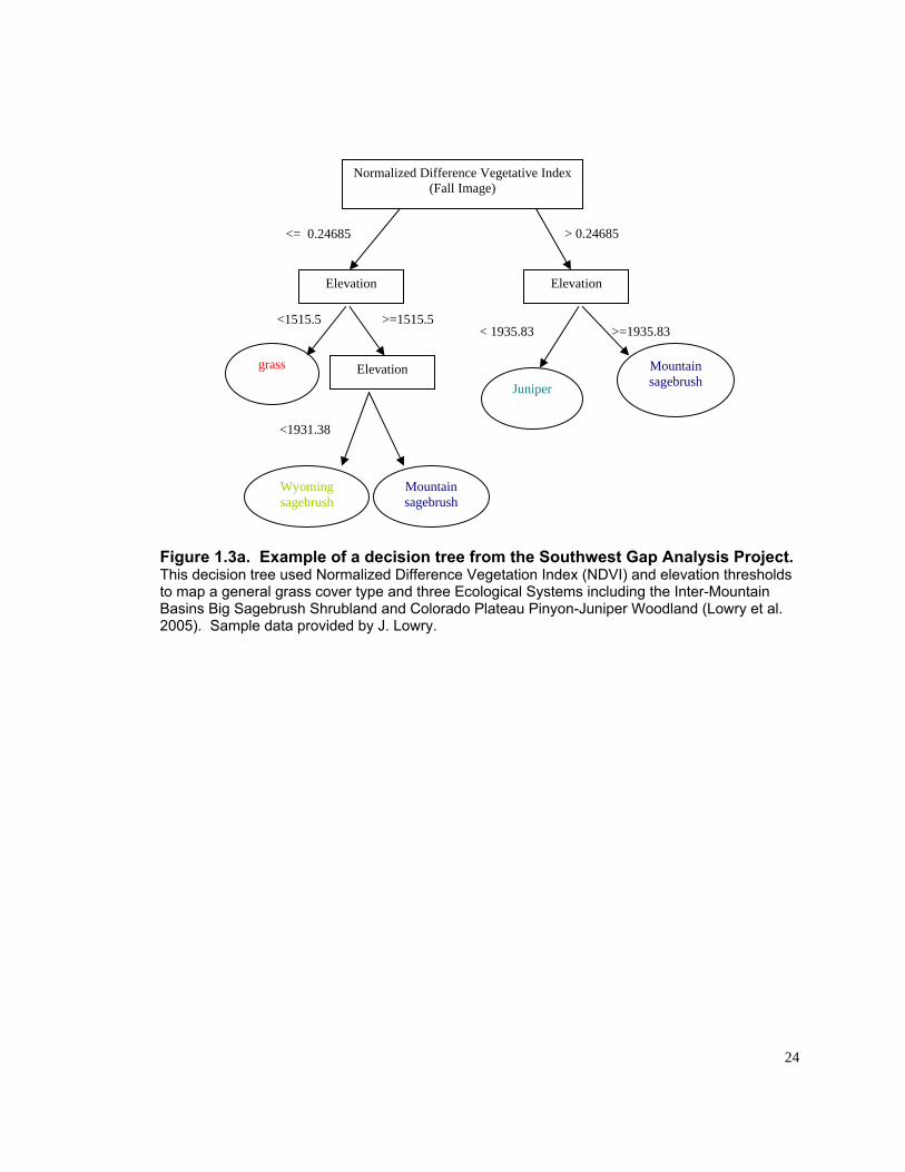
Figure 1.3a. Example of a decision tree from the Southwest Gap Analysis Project. This decision tree used Normalized Difference Vegetation Index (NDVI) and elevation thresholds to map a general grass cover type and three Ecological Systems including the Inter-Mountain Basins Big Sagebrush Shrubland and Colorado Plateau Pinyon-Juniper Woodland (Lowry et al. 2005). Sample data provided by J. Lowry.
>=1935.83
Normalized Difference Vegetative Index (Fall Image)
Juniper
Mountain sagebrush
Wyoming sagebrush
Elevation
Elevation
> 0.24685<= 0.24685
Elevation
grass
Mountain sagebrush
<1515.5 >=1515.5 < 1935.83
<1931.38
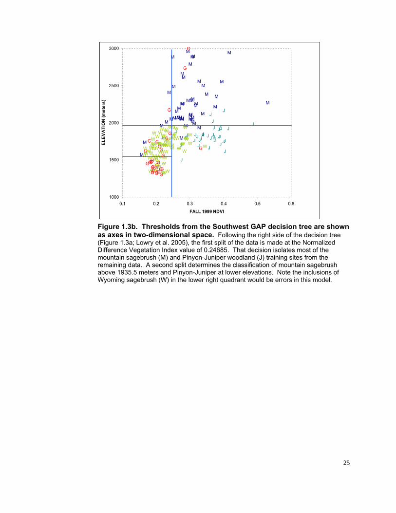
25
G
G
G
GGG G
G GGGG
GGGG GG GGGG GGGG
JJJ JJJ J JJJ JJJ JJ J JJ JJ JJJJ J J JJJ JJ JJJJ J J
J
J
M MMM M
M
MM
M MMM
M M MMMM MM MM M MMM MMMMM MMM MMM M MMMM MM M M
MM
M
WW WWWWWWW W WWWWW WW WW WWWWWWWW WW WWW WWW WW WW WW W WW W WW WWWWWWW WWWW WW WW WWWWW WWW
1000
1500
2000
2500
3000
0.1 0.2 0.3 0.4 0.5 0.6
FALL 1999 NDVI
ELEV
ATI
ON
(met
ers)
GGG G G
W W
Figure 1.3b. Thresholds from the Southwest GAP decision tree are shown as axes in two-dimensional space. Following the right side of the decision tree (Figure 1.3a; Lowry et al. 2005), the first split of the data is made at the Normalized Difference Vegetation Index value of 0.24685. That decision isolates most of the mountain sagebrush (M) and Pinyon-Juniper woodland (J) training sites from the remaining data. A second split determines the classification of mountain sagebrush above 1935.5 meters and Pinyon-Juniper at lower elevations. Note the inclusions of Wyoming sagebrush (W) in the lower right quadrant would be errors in this model.
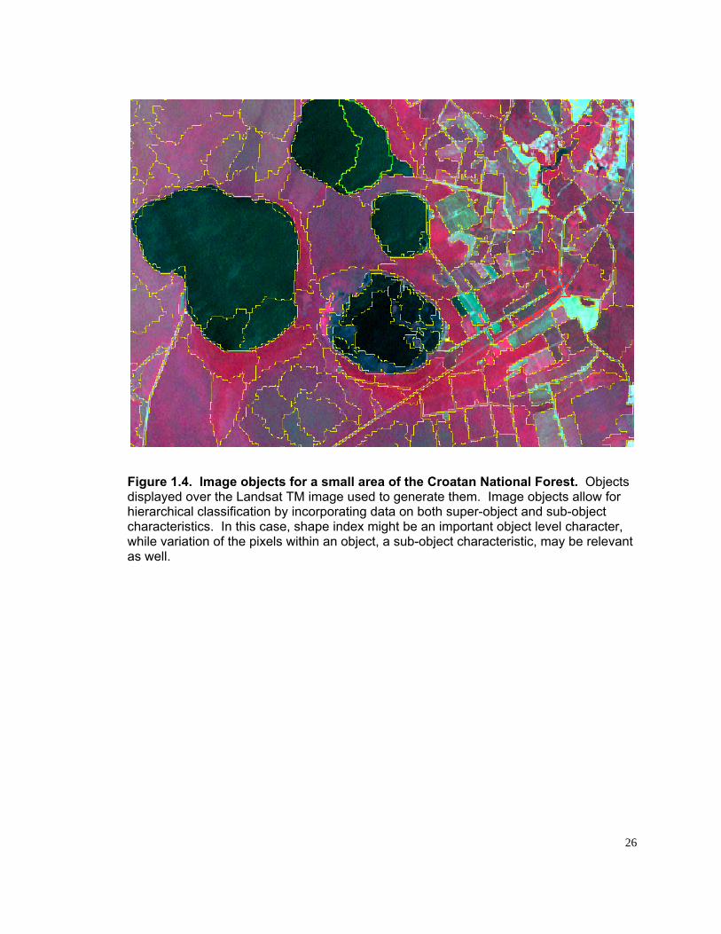
Atlantic Coastal Plain Peatland Pocosin
Atlantic Coastal Plain Nonriverine Swamp and Wet Hardwood Forest
Planted Pine
Open Water
>=1931.38
Figure 1.4. Image objects for a small area of the Croatan National Forest. Objects displayed over the Landsat TM image used to generate them. Image objects allow for hierarchical classification by incorporating data on both super-object and sub-object characteristics. In this case, shape index might be an important object level character, while variation of the pixels within an object, a sub-object characteristic, may be relevant as well.
26
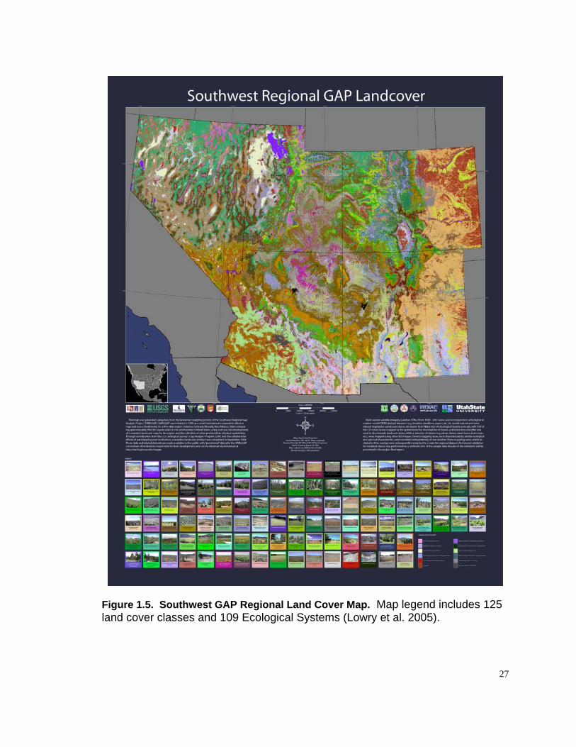
Figure 1.5. Southwest GAP Regional Land Cover Map. Map legend includes 125 land cover classes and 109 Ecological Systems (Lowry et al. 2005).
27
28
Case Study: Southwest GAP Project Regional Land Cover Map (Lowry et al. 2005). In this case we highlight the series of choices made by the Southwest Gap Analysis
Project for mapping vegetation over a 5 state area. The final map, shown below,
includes 125 map classes, with 109 Ecological Systems represented (Figure 1.5).
Target Map Classes: For this project a total of 109 Ecological Systems were mapped.
Prior to mapping, extensive field work was done to collect vegetation data that would
inform the classification system, as well as act as training and assessment data. For a
complete description of the 109 map classes based on the Ecological Systems
Classification or to download the data, see the Southwest GAP land cover report
(http://earth.gis.usu.edu/swgap/landcover.html).
Automated vs. Manual Delineation: The decision tree process used for this project is
an automated supervised classification method. The training data provide the a priori
class labels, and the decision tree model determines the best series of binary splits of
the data to predict the labels based on those training data. In this case, over 93,000
training data points were gathered; 20% of those points within each target map class
were randomly selected and set aside for the final accuracy assessment, and the
remaining 80% were used to “train” the decision tree.
Satellite-based mapping: The base imagery for the project was Landsat Enhanced
Thematic Mapper (ETM) imagery acquired within a three year time period (1999 to
2001).
Multi-temporal imagery: In order to take advantage of seasonality, three seasons
(spring, summer, and fall) of images were used. A total of 237 Landsat scenes were
required to cover the study area for the three seasons.
29
Integrating Ancillary Data with remote sensing: Landsat ETM satellite images and
image derivatives, including the Normalized Difference Vegetation Index and tasseled
cap brightness, greenness, and wetness indices, were used in the decision tree
modeling.
Digital Elevation Models (DEM) and derivatives including slope, aspect and landform.
In this study the researchers had compiled data including geology, State Soil
Geographic Database (STATSGO), and 1x1km meterologic data, but decided not to
include those data in the modeling because of differences in the scale of the satellite
data and those data sources.
Image stratification: Twenty five distinct mapping zones were developed for the
project. Each mapping zone was treated independently, and once completed, all zones
were mosaicked to create the final regional product.
Decision tree modeling: For each mapping zone, decision tree modeling was used to
map the natural vegetation of the zone. Non-modeled classes included land cover types
such as agriculture, developed, and water. For the modeled classes, the training data
were used as the response variables in a decision tree process, with the satellite
imagery and ancillary data sources described above as the predictor variables.
Lowry, J. H. Jr., R. D. Ramsey, K. Boykin, D. Bradford, P. Comer, S. Falzarano, W. Kepner, J. Kirby, L. Langs, J. Prior-Magee, G. Manis, L. O’Brien, K. Pohs, W. Rieth, T. Sajwaj, S. Schrader, K. A. Thomas, D. Schrupp, K. Schulz, B. Thompson, C. Wallace, C. Velasquez, E. Waller, and B. Wolk. 2005. The Southwest Regional Gap Analysis Project Final Report on land cover mapping methods. Report to the U.S.G.S Biological Resources Division. National Gap Analysis Program. 50 pp. (http://ftp.nr.usu.edu/swgap/swregap_landcover_report.pdf)
Manis, G. C. Homer, D. Ramsey, J. Lowry, T. Sajwaj, and S. Graves. 2000. The development of mapping zones to assist in land cover mapping over large geographic areas: A case study of the Southwest ReGAP Project. National Gap Analysis Bulletin. Bulletin No. 9. http://www.gap.uidaho.edu/Bulletins/9/bulletin9/bulletin9html/tdomzailcmolga.html#t6
30
Mapping Ecological Systems in the Coastal Plain of North Carolina. Alexa J. McKerrow1, Thomas R. Wentworth2, and Heather M. Cheshire3. 1 Southeast Gap Analysis Project, Department of Zoology, North Carolina State University, Raleigh, NC 27695-7617 ([email protected]); 2 Department of Plant Biology, North Carolina State University 27695-7612 ([email protected]); 3 Department of Forestry and Natural Resources, North Carolina State University 27695-8808 ([email protected]) Abstract Many of the plant communities of North America are in decline, due to a variety of
stresses including land use change, climate change, and plant pests, diseases, and
decline syndromes. Accurate maps of the current extent of those communities will
enhance our ability to assess their true status and will provide a baseline for monitoring
future changes. The U.S. National Gap Analysis Program has been working on regional
projects to test methods for mapping and modeling plant communities to create a
consistent and ecologically meaningful land cover map of the U.S. In this project, our
goal was to test methods for mapping and modeling Ecological Systems in the Coastal
Plain of the southeastern U.S. Specifically we were interested in testing the application
of image stratification and decision tree modeling for mapping the Ecological Systems in
the Onslow Bight region of North Carolina. We were also able to test the influence of
county level (SSURGO) and state level (STATSGO) soil data in decision tree modeling.
Decision tree modeling worked well for five of the six evergreen and nonriverine wetland
systems, but the Atlantic Coastal Plain Upland Longleaf System was not well mapped by
our method. The decision tree process performed best with the full complement of input
variables, and by testing the decision tree with and without the two levels of soils data,
we were able to observe an interaction between those two data layers in the modeling
process. The model in which both soils datasets were included predicted both the
occurrence of ecological systems that cover large extents and those that occur in
relatively small patches. Overall accuracy using conditional probabilities was estimated
at 77% and the Kappa statistic was 0.75. In general, by incorporating a variety of
techniques specific to the target map classes, we were able to successfully map most of
the Ecological Systems described by NatureServe for the Onslow Bight.
Keywords: Landsat TM, Ecological Systems, vegetation mapping, decision tree, pattern recognition, image objects.
31
Introduction We explored the challenges of mapping and modeling the vegetation of the coastal plain
region of the Southeastern U.S. The National Gap Analysis Program (GAP) has as its
mission “keeping common species common.” During the past decade, the program has
conducted and funded research in support of that mission. The overriding goal is
providing three key datasets that can be used to assess the conservation status of plant
communities and terrestrial vertebrate species in the United States: land cover,
vertebrate species distributions, and land management status. These layers have been
used to identify “gaps” in species protection by identifying areas that support vertebrate
species or plant communities that are currently under-represented in the conservation
network. The accuracy and thematic resolution of the land cover maps influence the
relevance of the analysis with respect to conservation and habitat modeling.
With that in mind, GAP has been focusing on the development of regionally consistent
and ecologically meaningful maps. The Southwest Gap Analysis Project has recently
completed a detailed land cover map for five southwestern states (Lowry et al. 2005).
The work described here is part of the ongoing Southeastern GAP, in which a land cover
map for nine states is being developed. While topographic relief and geology are drivers
of vegetation pattern in much of the U.S., the vegetation of the Coastal Plain is often
determined by underlying soils and hydrologic processes. Accurately mapping
vegetation in the low relief, highly diverse landscape of the Coastal Plain is challenging
because of the limited resolution in the elevation data available nationwide. We chose
the Onslow Bight for this project because of our ongoing collaboration with The Nature
Conservancy on a Landfire Pilot Project. This collaboration would provide a meaningful
test of the applicability of the map legend, as well as the final map.
The Atlantic Coastal Plain supports a diverse mosaic of vegetation, including maritime
forests and associated beach communities, upland longleaf pine woodlands, pocosins,
and riverine and nonriverine wetland communities (Wells 1928, Schafale and Weakley
1990). Soils, hydrologic processes, and disturbance (specifically fire, tides, and salt
spray) are primary factors in determining patterns in the vegetation of the Coastal Plain
(Wells 1928, Wells and Shunk 1938, Boyce 1954, Kologiski 1977, Komarek 1968,
Christensen 1988).
32
In addition to the complexity of the vegetation, the long history of human settlement and
the rapid rate of land use change make mapping the natural communities in the region
especially challenging. According to a World Wildlife Fund assessment (Ricketts et al.
1999) the Atlantic Coastal Plain of the Carolinas is an endangered ecological region in
need of “immediate protection of remaining habitat and extensive restoration.” These
authors estimated that only about 12% of the Mid-Atlantic Coastal Plain habitats can be
considered intact. Wyant et al. (1991) suggested that anthropogenic disturbance (timber
harvest and fire suppression) will continue to have the greatest influence on the extent
and composition of the forests of the Coastal Plain of North Carolina.
Study Objectives Our objective was to develop an effective methodology for mapping Ecological Systems
of the Atlantic Coastal Plain. Two immediate uses of that map would be a conservation
assessment of the Ecological Systems of the area and input into modeling predicted
distributions of vertebrate species. The goals of the study included 1) testing the
application of the Ecological Systems Classification in mapping in a ecologically diverse
but topographically homogeneous area, 2) testing the use of decision tree modeling for
mapping Ecological Systems, and 3) quantifying the impact of including soils data, both
county-level (SSURGO) and state-level (STATSGO) in the modeling process.
The Ecological Systems Classification was recently developed (Comer et al. 2003) in
response to a need for a nationally consistent vegetation classification system that could
be used as the target map legend for large area mapping. Previous mapping efforts in
the Southeast (Pearlstine et al. 1999) have shown that the coarse-scale resolution of
available imagery and the limited availability of ancillary datasets for mapping have
significantly limited our ability to map vegetation at fine levels of thematic detail. In this
work we wanted to test our ability to develop a map based on the Ecological Systems
Classification, using a hierarchical approach including image stratification with decision
tree modeling as the final step in that approach.
Specifically we wanted to examine the consequences of incorporating county-level soils
data, testing the hypothesis that these detailed data would improve the accuracy and/or
thematic resolution of the vegetation map. We were specifically interested in the
33
influence of the SSURGO data because it is not currently available nationwide, so we
wanted to understand the potential impact of not including it in our mapping efforts.
Background Status of the Dominant Plant Communities in the Atlantic Coastal Plain.
There are seven dominant plant communities in the Atlantic Coastal Plain, all of which
are decreasing in area, some more drastically than others. A summary of the current
status of each of those communities follows.
Longleaf Pine The longleaf pine (Pinus palustris) ecosystem is one of the best known examples of an
endangered ecosystem in the coastal plain (Jose et al. 2006, Noss et al. 1995, Ware et
al. 1993, Noss 1988). The factors that led to its decline include timber harvest,
agricultural clearing, grazing, free ranging hogs, and turpentine production (Frost 1995).
More recently, fire suppression and the associated invasion of hardwoods has led to a
decline in the remaining longleaf stands. Less than 2% of the original distribution of
longleaf remains, with less than half of that being managed with prescribed fire (Frost
2006).
Pocosin One of the distinctive plant communities of the Atlantic Coastal Plain is the peatland
pocosin. This nonriverine wetland community often has an open canopy of Pond Pine
(Pinus serotina) and a dense evergreen shrub understory (Kologiski 1977, Wells 1928).
Historically, pocosins are thought to have occupied as much as 908,000 hectares in
North Carolina (Wilson 1962, Richardson 1981). In 1989, 608,000 hectares of pocosin
remained, half of which could be characterized as being in a natural state (Richardson
and Gibbons 1993). Thus two thirds of the original extent for this plant community has
been lost or severely degraded.
Nonriverine Wet Hardwood Forest Another threatened plant community of the Coastal Plain Region is the nonriverine wet
hardwood forest. Based on extensive field survey data, Schafale (1999) estimated a
loss of 1730 hectares of this community between 1990 and 1999. That represents a
34
loss of 52% of its known 1989 extent. To estimate the potential presettlement extent,
Schafale (1999) identified the soil series known to support nonriverine wet hardwood
forest in Currituck and Hyde counties. Schafale restricted that analysis to soils well
documented with respect to supporting the nonriverine forests and, thus is likely
underestimating the true presettlement representation. The total area of the suitable
soils was 16,300 hectares (40,278 acres) and the total area of known sites supporting
the forest in 1998 was 556 hectares (1373 acres) meaning that as little as 3.4 percent of
the original extent remains.
Atlantic White-cedar Forest Atlantic White-cedar forest is another critically endangered wetland type that occurs in
the coastal plain of North Carolina (Noss et al. 1995). In his review, Frost (1987) was
able to document records of this community throughout most of the Coastal Plain
counties of North Carolina, and Ashe (1894) estimated that it covered 80,940 hectares.
In a 1997 inventory, any stand over 1.6 hectares (4 acres) that had Atlantic White-cedar
in the canopy was reported (Davis and Daniels 1997). The greatest remaining
concentrations occurred in the counties adjacent to the Dare Peninsula.
Maritime Communities Maritime forest and associated dune communities occur throughout the barrier islands of
North Carolina. In these forests, the broad-leafed evergreen trees, live oak (Quercus
virginiana) and upland laurel oak (also known as sand laurel oak or Darlington Oak (Q.
hemisphaerica)), often co-occur with loblolly pine (Pinus taeda). These systems have
been affected throughout their range by coastal development. Less than half of the
remaining maritime forests in the southeast are within the conservation network (DeVivo
et al. 2005). The dynamic nature of barrier islands means that even systems within the
conservation network are threatened. Under normal conditions these island
communities are constantly shifting over time, invading newly accreted sands and being
reduced on the eroding sides of barrier islands (Bellis 1980, Bourdeau and Oosting
1959). These processes can occur slowly in response to the geomorphologic processes
or can occur more rapidly with differential re-establishment of the plant communities
following a storm event. As urban development continues, the ability of the natural
systems to migrate with the changing landscape becomes more limited. Continuing sea
35
level rise, possibly exacerbated by global climate change, will intensify the threats to
coastal communities.
Bottomland Forests Harris et al. (1984) estimated a loss of 78% of the original extent of bottomland forests in
the Southeastern United States. Wetland classification has not traditionally made a
distinction between floodplain forests and nonriverine wetland forests, which makes
estimating the loss for the bottomland types difficult. When considering all palustrine
forested wetlands, Hefner and Brown (1985) estimated that 92% of the 2.2 million
hectares lost in the 20 years prior to the mid-1970s occurred in the Southeast. Between
the mid-1970s and mid-1980s it is estimated that North Carolina lost more than 40,469
hectares (100,000 acres) of palustrine forested wetland (Dahl et al. 1991).
Carolina Bays Carolina bays are a unique type of isolated wetland that occur in the outer Atlantic
Coastal Plain from New Jersey to Florida (Sharitz 2003), with the greatest
concentrations in the Carolinas. Because of their geomorphology the bays are
recognizable from space as elliptical basins of wetlands within a matrix of upland. The
substrate, either peat or clay-based, influences the plant communities they support
(Schafale and Weakley 1990). Historically, many of these wetlands have been drained
for conversion to agriculture or tree plantations. More recently, the interpretation of the
Clean Water Act that removes these wetlands from protection makes Carolina bays
especially vulnerable (Sharitz 2003). Estimates of the historic number of bays vary
widely, making it difficult to estimate the proportion that has been lost (Richardson and
Gibbons 1993, Prouty 1952).
Previous Mapping Efforts in the Coastal Plain.
A variety of land cover maps with varying degrees of thematic and spatial detail exist for
the Coastal Plain of North Carolina. Most recently, the North Carolina GAP land cover
map (McKerrow et al. 2006) provides the first comprehensive coverage with a map
legend that emphasizes natural vegetation types. In that project, mapping of the
vegetation types in the coastal plain was based on detailed county-level soil survey
data, National Wetland Inventory Data (USFWS 2006), and Landsat TM imagery. In the
36
Onslow Bight portion of that land cover map, there are 39 cover types, 21 of which
represent natural vegetation types. The vegetation classification system used
(Pearlstine et al. 1999) was developed in collaboration with NatureServe and was a
precursor to the Ecological Systems Classification (Comer et al. 2003) currently being
used by GAP and other national mapping programs.
Frost and Costanza (2006) mapped the presettlement vegetation of the Onslow Bight
Study area using county-level soils data and topography. The county level soils data
(SSURGO) were cross-walked based on expert opinion into 21 vegetation types, the
majority of those being variants on longleaf pine communities.
Lunetta et al. (2003) mapped the general land cover of the Neuse River Basin. The
southeastern portion of that river basin study area intersects the Onslow Bight. In that
classification, Satellite Pour l'Observation de la Terre (SPOT) and Landsat Enhanced
Thematic Mappter (ETM) imagery were used in combination with ancillary datasets to
map land cover. To classify crops (corn, tobacco, cotton, soybean, and hay/pasture) the
authors used differences in the Normalized Difference Vegetation Index (NDVI) from two
time periods. Vegetation types were limited to Anderson Level II type classes (e.g.,
forested wetlands, deciduous forest).
The Center for Geographic Information and Analysis in North Carolina contracted with
EarthSat Corporation to produce a statewide land cover map in 1996. That
classification included more detail in the vegetation types, with descriptions of most
classes being based on physiognomy (e.g., broadleaf evergreen forest), and a few being
based on general biogeography (e.g., mountain conifer) or the dominant species mix
(e.g., oak/gum/cypress). The statewide map included 23 land cover classes (EarthSat
1997).
Zhu and Evans (1994) mapped the forest types of the coterminous U.S. using 1- by 1-
km Advanced Very High Resolution Radiometer (AVHRR) imagery. Four forest types
based on the Society of American Foresters (SAF) classification were mapped in the
Atlantic Coastal Plain region (Oak - Gum - Cypress, Oak - Pine, Loblolly - Shortleaf -
Pine, and Longleaf - Slash Pine).
37
Richardson (1981) developed a map of the pocosins and Carolina bays of North
Carolina, and Schafale (1999) has developed a map of nonriverine wet hardwood
forests. Aerial photo interpretation was used for mapping both of these high
conservation priority vegetation types.
Methods Study site
We included the thirteen counties that intersect the Onslow Bight Landscape as defined
by The Nature Conservancy Onslow Bight Rapid Assessment Pilot Project (Figure 2.1).
The area covers approximate 250,000 km2 and intersects portions of the Atlantic
Coastal Flatwoods Section and the Coastal Plains and Flatwoods Lower Section of the
Forest Service’s Ecological Regions Map (Keys and Carpenter 1995). With respect to
ecological regions as described by Omernik (EPA 2004), the majority of the study area
occurs within the Middle Atlantic Coastal Plain, with a small fraction overlapping the
Southeastern Plains Region. Relief in the region is minimal, peaking at 50 meters with
most of the area being under 15 meters above sea level. The northeastern corner of the
study area was partially submerged in the post-glacial period and is referred to as the
embayed region (Robinson 1979). To the south, marine terraces are considered to be a
region of emergence, making swamps less common and creating conditions for defined
river valleys. The vegetation represents a complex mosaic of wetland and upland plant
communities, many of which are fire dependent.
Target Map Classes
We adopted the NatureServe Ecological Systems Classification (Comer et al. 2003) as
our target map legend. The goal for the Southeast Regional GAP is a regionally
consistent land cover map and this classification was designed as an ecologically
meaningful classification that could be mapped using mid-scale remotely sensed data.
There are 25 Ecological Systems in the Atlantic Coastal Plain Region of North Carolina
(Table 2.1). Each Ecological System is attributed with a landscape pattern (matrix,
linear, large or small patch) that describes the spatial extent and configuration of that
system. For example, the Atlantic Coastal Plain Longleaf Pine Woodland is considered
a matrix system, meaning it historically occurred throughout the landscape with other
38
systems (linear, large patch and small patch) embedded within it. Complete
descriptions for each of the Ecological Systems are available through the NatureServe
Explorer Encyclopedia (www.natureserve.org/explorer).
For a few of the Ecological Systems, we added modifiers to describe variations in
vegetation structure that occur within that type. For example, we identified three
potential modifiers of the Atlantic Coastal Plain Nonriverine Swamp and Wet Hardwood
Forest (Taxodium, Oak, and Atlantic White-cedar dominated) representing common
cover type variants in the dominant canopy species resulting from hydrologic regime and
fire history. In addition to the vegetation types, some modified classes from the National
Land Cover Dataset (NLCD; Homer et al. 2007) were added to make the land cover
classification more meaningful for habitat modeling. A range map for each of the
Ecological Systems to be mapped was created by NatureServe ecologists for the
Southeast GAP. These ranges were based primarily on the linework in Omernik’s
ecoregional coverage (EPA 2004), but in some cases delineations were made based on
the range of one of the dominant canopy species in examples of the Ecological System.
Satellite Imagery and Ancillary Data
Landsat TM We used Landsat TM image mosaics created at the U.S.G.S. Earth Resources
Observation Systems Data Center (EDC) as a part of the National Land Cover Dataset
national mapping effort (Homer et al. 2001, Homer et al. 2002). In that effort, the U.S.
was divided into a series of mapping zones and each zone was mapped independently.
The zones were delineated based on five criteria - size, physiography, land cover
patterns, spectral patterns, and natural breaks in land cover that would facilitate edge
matching of the map zones (Homer and Gallant 2001). This delineation method
overcomes some of the issues of heterogeneity often encountered when the study area
is defined using political (e.g., state) boundaries. For Ecological Systems level mapping,
even these zones can be relatively heterogeneous. For example, the mosaic for
mapping zone 58 (Atlantic Coastal Plain of North and South Carolina) includes a variety
of vegetation types from maritime forests to Sandhills longleaf pine woodlands. We dealt
with that variability by further dividing the study area into subzones.
39
Preprocessing at EDC included identification of three target image dates using multi-
temporal normalized difference vegetation index (NDVI; Yang et al. 2001) to guide the
selection of the imagery for three seasons (leaf on, leaf off and spring). Once the range
of target dates was identified, the analysts created seasonal mosaics. In cases where
the images from the target dates were of poor quality, imagery from the same season in
an alternate year was selected.
Portions of 14 Landsat TM images were used to create the image mosaics for Zone 58,
with dates ranging from September 1999 to as late as June 2002 (Table 2.2). For each
of the seasonal mosaics both the 6 reflectance bands and a three-band (brightness,
wetness, and greenness) tasseled cap transformed images were used. This was the
case in both the NLCD 2001 mapping effort for this zone, as well as for this study
(Huang et al. 2002). For a complete discussion of the preprocessing steps taken at
EDC see Homer et al. 2002.
Land Cover, Impervious Surface, and Canopy Closure The Southeast Gap Analysis Project had previously collaborated with U.S.G.S. in the
development of the NLCD 2001 database (Homer et al. 2007). A sixteen class land
cover map was produced using hierarchical decision tree modeling at the Biodiversity
and Spatial Information Center (BaSIC) at North Carolina State University (U.S.G.S.
2003b). The Impervious and Canopy closure estimates were modeled using sub-pixel
classification and regression tree modeling at the Natural Resource and Spatial Analysis
Laboratory (NARSAL) at the University of Georgia (USGS 2003a and c). Each of the
three datasets was based on the same Landsat TM mosaics described above. In Zone
58, we included additional wetland categories consistent with the mapping of palustrine
and estuarine types used by the Coastal Change Analysis Programs map legend
(NOAA – CCAP 2006; Table 2.3).
We used the NLCD 2001 land cover both as an input layer for mapping some of the
Ecological Systems, as well as for masking the anthropogenic types. Canopy closure
was used as an input into modeling of managed evergreen cover as well as in the
decision tree modeling for several of the Ecological Systems.
40
Soils We derived two soils datasets from the Natural Resource Conservation Service to be
used as inputs into the modeling process. The State Soil Geographic Database
(STATSGO) is a national database developed at a 1:250,000 scale (NRCS 2007). For
each map unit in the STATSGO data, the component soil series and the percentage
representation for each of those series in the average soil unit is described in the
database. These soils maps were developed by generalizing existing soils information.
The Soil Survey Geographic Database (SSURGO) includes detailed county-level soil
series maps developed at a scale of 1:24,000 (NRCS 2007). From the SSURGO data
we calculated the average percentage organic matter for each soil series using the
official soil descriptions. To account for the contribution of organic matter, we adjusted
the percentage of each of the mineral fractions (sand, silt, and clay) by subtracting the
percent organic matter from 100 percent to determine a correction factor. We derived
the percentage sand, silt, and clays for each soil series by translating the soil texture
(loam, sandy loam, clay) based on the soil texture triangle (Soil Survey Staff 1990). The
adjustment to include organic matter in the soil texture calculation was then applied to
the sand, silt, and clay percentages, making the combination of sand, silt, clay, and
organic matter percentage total 100%. For each fraction a single data layer was
generated (see below).
Correction Factor for Mineral Fractions = 100 - Average % Organic Matter
Layer 1: Adjusted % sand = % sand * Correction
Layer 2: Adjusted % silt = % silt * Correction
Layer 3: Adjusted % clay = % clay * Correction
Layer 4: Average % Organic Matter
To develop the STATSGO data layers, we used the same process for determining the
percentage organic matter and the adjusted percentages for sand, silt, and clay for each
soil series. The proportional representation of each soil series in a STATSGO unit was
then used to weight the contribution of that series to the larger unit. The compositional
representation for soil series in each STATSGO unit is reported in the STATSGO
database. Our approach is similar to that taken to develop the CONUS-SOIL dataset
41
(www.soilinfo.psu.edu) developed for the conterminous U.S., but we have included
organic matter as a fourth soil fraction.
National Wetlands Inventory We used the National Wetland Inventory in the development of the NLCD 2001 for
mapping zone 58, which includes the Onslow Bight study area (U.S.G.S. 2003b). For
that effort two data layers were derived from the National Wetland Inventory Data (U.S.
F.W.S.): a wetland/upland layer and a layer that corresponded to general wetland
classes including palustrine wetlands (forest, shrub, and emergent) and estuarine
wetlands (forest, shrub, and emergent). These data layers were used as input layers for
decision tree modeling of the wetland vs. upland forest, shrub, and emergent land cover
classes for the NLCD 2001. We used an unsupervised classification based on the
spring imagery to refine the boundary at the palustrine/estuarine interface. For the
systems level mapping, these derived layers were used as input into the decision tree
modeling.
Landform We derived landforms using the National Elevation Dataset (NED) 30 meter elevation
data. Preprocessing steps included identifying areas with anomalies (e.g., striping) in
the elevation data, replacing those areas with other data if they were available and, if
not, using directional filtering. The landform calculations were modeled using the
approach outlined by Anderson et al. (1998).
Image Objects We used the pattern recognition software eCognition to segment the spring image
mosaic into objects. Object boundaries were determined through interactive
calculations of homogeneity. In each step the homogeneity of an object after being
merged with its neighbor was calculated; if the heterogeneity of the new object exceeds
the predetermined threshold level, the objects were not merged. Two indices of
homogeneity were used in image segmentation - color vs. shape and smoothness vs.
compactness - and they could be weighted by the analyst. In this study we used a color
parameter of 0.3 (scaled 0 to 1) and smoothness parameter of 0.5 (scaled 0 to 1). In
other words, we weighted spectral homogeneity slightly higher than shape homogeneity
42
and gave equal weighting to smoothness and compactness. The scale parameter
determined the size of the objects that can be generated and therefore determined the
threshold for the maximum heterogeneity allowed in an object (the higher the scale
parameter, the more heterogeneous the objects). In this case we used a scale
parameter of 30, which resulted in over 57,000 objects. For a technical discussion of
homogeneity calculations for color and shape indices see Zhong et al. (2005). Those
objects were used for delineating specific areas of interest, refining boundaries from
other datasets so they matched the spectral data, and as input in decision tree
modeling. Summary statistics for eight input variables were generated for each object
for use in modeling (Table 2.4).
Reference Data Training and assessment data were compiled from both field data and aerial photograph
interpretation. Digital aerial photographs acquired as a part of the Southeast Gap
Analysis Project were interpreted directly to Ecological Systems and their modifiers.
The North Carolina GAP reference points were relabeled based on a cross-walk from
that classification, an early version of a systems based classification (Pearlstine et al.
1999), to the current Ecological Systems classification. North Carolina Natural Heritage
Plant Community data and plot data from the North Carolina Vegetation Survey (Peet et
al. 1998) were incorporated by cross-walking the plant community labels to the
Ecological Systems (Table 2.5). All points were then carefully screened against the
2001 imagery and 1998 digital orthophoto quarter quads (DOQQs) to check for land
cover changes and to apply modifiers to the appropriate classes. Finally, areas with few
or no training data reference points were photo interpreted. Once the reference data
were compiled, they were stratified by ecological system or cover class and a random
sample of at least 25% of the points was removed for use in the final assessment.
Ecological Systems and Managed Pine Mapping
Riverine Systems We mapped the riverine Ecological Systems by intersecting the National Hydrologic
Dataset (NHD) streams with image objects derived in eCognition. The object generation
was done for the entire study area so the patterns derived from the imagery would be
43
consistent for the entire length of a river or stream. Final editing was done manually to
add objects missed by the NHD stream data and to remove objects that were dominated
by successional or anthropogenic vegetation types (clearcuts, plantations). Pixels
representing non-vegetated types (urban, agriculture, barren) were then removed,
leaving only the vegetated pixels within the stream or river corridor.
Once the floodplain areas had been mapped, the hydrology data were used to classify
the Ecological Systems based on flow accumulation and water type. Using the DEM
and NHD data, the flow accumulation for each stream segment was calculated in
ArcGIS. In order to “force” the modeled flow to follow the NHD stream network, the
streams were “burned” into the DEM prior to calculating the flow accumulation. More
specifically, the elevation for any grid cell that intersected a stream was lowered by 100
meters. A threshold based on the number of grid cells contributing to the flow at each
point along the stream network was then used to create three categories of streams:
small stream (< 100,000), river (100,000 – 1,000,000), and large river (> 1,000,000).
Finally, streams and rivers were characterized by water type, blackwater or brownwater.
Streams originating in the coastal plain tend to be black water, while those originating in
the Piedmont tend to be brownwater, with a higher sediment load (Schafale and
Weakley 1990). A blackwater/brownwater classification of streams was done for the
entire Coastal Plain, with all streams or rivers originating in the coastal plain being
classed as blackwater, and those with origins in the Piedmont being classed as
brownwater. In a few cases, sufficient flow contributed from coastal streams overcomes
the fact that a river originated in the Piedmont. We used the literature and expert review
to reclassify portions of these rivers as blackwater.
By intersecting river size with water type, five riverine systems were mapped:
• Atlantic Coastal Plain Large River Floodplain – Brownwater Modifier
• Atlantic Coastal Plain Large River Floodplain – Blackwater Modifier
• Atlantic Coastal Plain Blackwater Stream Floodplain Forest
• Atlantic Coastal Plain Brownwater Stream Floodplain Forest
• Atlantic Coastal Plain Small Brownwater River Floodplain Forest
44
Maritime Systems The coast of North Carolina presents a unique set of mapping challenges. The barrier
islands and coastline along the mainland represent relatively small acreages with a
distinct suite of plant communities. Maritime forest, dunes and grasslands, tidal swamp
forests, and marshes all co-occur in relatively small patches and are often intermixed
with urban cover types. In order to map the Ecological Systems along the coast, an
area of interest was created using the image objects previously described and
Omernik’s ecoregional boundaries (EPA 2004). A 3 km buffered version of the Carolina
Barrier Islands and Coastal Marshes ecoregion was intersected with the image objects
to create the subzone for mapping. By selecting objects as the new linework, boundary
issues between the coarse scale ecoregional linework and the imagery were minimized.
At the same time, the image objects tied the new line work and boundaries to the base
imagery, which was important along the coast, where the shapes of the islands are
changing over time.
By restricting the area being mapped, the number of map classes within the maritime
area of interest was limited, making it possible to recode from the detailed version of the
NLCD 2001 land cover classification. For example, upland evergreen forests were
recoded as Atlantic Coastal Plain Southern Maritime Forest and estuarine forested
wetlands were recoded as Atlantic Coastal Plain Tidal Wooded Swamp. The barren
classes were mapped by manually delineating areas to be recoded based on location.
For example, barren land and grassland herbaceous pixels along the outer coast were
recoded to the Atlantic Coastal Plain Southern Dune and Maritime Grassland, while
inland barren land was mapped as either bare sand, bare soil, or mines (see Inland
Barren Classes).
There were five dominant Ecological Systems mapped in the maritime region:
• Atlantic Coastal Plain Central Salt and Brackish Marsh
• Atlantic Coastal Plain Embayed Region Tidal Salt Marsh
• Atlantic Coastal Plain Central Maritime Forest
• Atlantic Coastal Plain Southern Dune and Maritime Grassland
• Atlantic Coastal Plain Southern Tidal Wooded Swamp
45
Upland Deciduous Forests Landforms were used to separate the Atlantic Coastal Plain Mesic Hardwood and Mixed
Forest from Atlantic Coastal Plain Dry and Dry-Mesic Oak Forest. If the NLCD 2001
land cover was deciduous or mixed forest and the landform was slope crest, flat summit,
North/Northeast side slopes, or North/Northeast cove/ravine then it was mapped as the
ACP Mesic Hardwood and Mixed Forest. All remaining deciduous forests were
classified as ACP Dry and Dry-Mesic Oak Forest. Given the lack of topography in the
coastal plain, the vast majority of the study area was modeled as dry or moist flats. Two
distinct exceptions occurred along the bluffs of the Cape Fear and Neuse River, where
small patches met the criteria for this decision rule.
Atlantic White-cedar Although the Atlantic White-cedar Forest was not treated as a distinct Ecological
System, it has been recognized by others as a distinct plant community (Schafale and
Weakley 1990) and is considered to be critically endangered (Noss et al. 1995). We
therefore decided to map it as a modifier of the Atlantic Coastal Plain Nonriverine
Swamp and Wet Hardwood Forest. In the current Ecological Systems Classification,
Peatland Atlantic White-cedar Forest is proposed as a provisional Ecological System.
We mapped this type using aerial photo interpretation with color infrared digital
orthophoto quarter quads (DOQQs) as the base layer. While most of the Atlantic White-
cedar Forest in North Carolina occurs north of the Onslow Bight, several small patches
were mapped in the Green Swamp of Brunswick County.
Natural Lakeshores There are five natural lakes in the Onslow Bight study area. Three of those lakes have
occurrences of the Southeastern Coastal Plain Natural Lakeshore. To map those sites,
the leaf off tasseled cap image mosaic was used to generate image objects in
eCognition (scale 5, shape index 0.1, compactness 0.7) and the objects at the
land/water interface with mixed pixel signature were labeled as lakeshore.
Carolina Bays Carolina Bays were photo-interpreted using DOQQs as the base imagery. The
dominant land cover from the NLCD 2001 within each bay was then used to distinguish
46
the Atlantic Coastal Plain Clay-Based Carolina Bay Wetland from the Atlantic Coastal
Plain Peatland Pocosin -Carolina Bay Wetland. Bays dominated by deciduous wetland
forest or water were mapped as clay-based, while those dominated by evergreen
wetland forest or shrubs were mapped as the peatland type. We chose not to use the
underlying soils data to define clay-based vs. peatland, because altered hydrology or fire
regime can result in a shift to a more evergreen dominated community (Schafale and
Weakley 1990), although the rate and likelihood of that change is poorly understood.
Managed vs. Natural Evergreen Prior to mapping natural systems, the managed pine stands throughout the mapping
zone were classified using a decision tree model. Pixels mapped in NLCD 2001 as
evergreen forests were subset from the leaf off tasseled cap image mosaic and forty
clusters were generated using Imagine Isodata algorithm (Lieca 2003). A stratified
random sample of 750 points was then generated based on those clusters for photo-
interpretation. The stratification by clusters was done to ensure even coverage of
interpreted points throughout the different images in the mosaic and throughout the
range of conditions for evergreen forests. Each of the 750 points was located on 1998
DOQQs and interpreted as managed or natural. In cases where the cover class in the
DOQQ was not evergreen or the point was near a boundary with a non-evergreen type,
that point was discarded. In all, 679 points (320 managed, 359 natural) were labeled for
use in decision tree modeling.
See5 software (RuleQuest Research Release 2.02; Quinlan 1993) was used in the
decision tree modeling process. The datalayers used in modeling managed vs. natural
evergreen for zone 58 are listed in Table 2.4. In addition to the imagery inputs, image
objects generated in eCognition were included with 8 context variables. Object specific
mean canopy closure, area, shape index, compactness, border length, as well as mean
leaf off tasseled cap brightness (band 1), standard deviation of the leaf off tasseled cap
brightness, and mean spring tasseled cap brightness were included as inputs.
The decision tree classifier was run with all 679 points, with boosting (10 trials).
Boosting is an interactive classification process in which each of the previous run trials is
used to identify which training data records are incorrectly classified. A weighting
47
scheme is then used to prioritize decisions that will correctly classify those records in the
current trial. For each trial 10% of the points were removed and used in the cross
validation for the model. Once the decision trees had been generated, the See5
Classifier version 2.02 was used to translate the decision trees into maps of managed
vs. natural evergreen forest.
Evergreen and Nonriverine Ecological Systems After removing the previously mapped or modeled Ecological Systems and
anthropogenic types, there were six forested systems to be mapped (Table 2.6). For
these forest types, we had a total of 548 points in the Onslow Bight study area. Of
those, 248 were set aside for model assessment and 300 were used as training data in
a decision tree modeling process.
RuleQuest See5 software was used to test both the decision tree modeling approach
and the effects of including a variety of input data layers for mapping these Ecological
Systems. Input layers available for modeling are listed in Table 2.4. In each case the
See5 Classifier was run with boosting of 10 trials, global pruning of 25%, and a minimum
of 2 cases per terminal leaf. Cross-validation was not used because of the limited
number of samples for each of the Ecological Systems being mapped and because the
independent assessment was to be run.
In order to assess the influence of several of the key data layers we ran multiple
classifications and varied the input layers included in the model. Of primary interest was
the influence of the state level STATSGO soils data, as well as the county level
SSURGO data. We ran five variations of the classification including 1) Full model, all
input layers were included; 2) No STATSGO, the four texture bands from the state level
soils data were also excluded (% sand, % silt, % clay, % organic matter), but all other
input layers were the same; 3) No SSURGO, the county level soils data layers were
excluded; 4) No STATSGO and No SSURGO, all layers derived from soils data were
excluded; and finally 5) No datasets derived from vector data, including soils, National
Wetland Inventory, and Image Objects were included in the models. Without vector
48
inputs, the final model would be reliant on imagery and land cover derived from imagery
alone. Each decision tree generated was then applied to create a map of the Ecological
Systems to be assessed.
Inland Barren Classes Mines and unconsolidated shore were recoded from the NCLD 2001 barren class using
an area of interest. The remaining barren pixels were then classified as bare sand if the
reflectance in the leaf on tasseled cap brightness band was greater than 80. Lower
reflectance pixels were mapped as bare soil.
Successional Shrub and Herbaceous Classes We used an unsupervised classification to identify transitional vegetation across zone
58. Clusters were generated from the spring and leaf on image mosaics using the
Imagine Isodata algorithm and labeled as transitional based on photo interpretation for
each of the clusters. Those pixels were then clumped to create two patch sizes (2 and
10 hectares). The greenness band from the spring image mosaic was then subtracted
from the greenness band of the leafon image mosaic to create a greenness difference
image. Small patches that showed a relatively large decrease in greenness (< - 14.5)
and large patches with any loss (< 0) were classified as clearcut shrub or clearcut
herbaceous. Shrub and herbaceous pixels not mapped as clearcuts were then labeled
as other herbaceous or other shrubland.
Salt/Brackish vs. Fresh Water The National Wetland Inventory palustrine/estuarine wetlands data were used as a
guide for manually delineating the split between the salt/brackish water and freshwater.
In the NLCD 2001 land cover there were many emergent wetland pixels scattered
throughout the study area. A large number of those represented wet areas within
agricultural fields or other anthropogenic cover classes and not “true” wetlands. We
allowed those pixels to be recoded based on the majority membership in the image
object in which they occurred. For example, palustrine emergent within an object with a
majority of member pixels classed as Large River Blackwater Forest was recoded to
49
Large River Blackwater Herbaceous. In another example, objects dominated by
herbaceous clearcut pixels would be recoded as herbaceous clear cut.
Post Processing Individual map classes from the processes described above were combined with the
NLCD 2001 urban and agricultural classes to create final land cover map. We then
used Smart Eliminate (Ver. 1.0) within the NLCD Mapping Tool to generate the final map
with a minimum mapping unit of 4 pixels (0.5 hectares).
Accuracy Assessment
The models for the evergreen forest and woodland systems were assessed with 248
independent data points that had been set aside prior to modeling. Plant community
data from the Natural Heritage Program has been gathered based on inventories for
specific plant communities, so we assumed a stratified random sampling design in our
assessment. In order to account for the variation in the acreage of the Ecological
Systems and the number of assessment points, we used marginal frequencies to
estimate map accuracy (Card 1982, Stehman 1997). Formulas for estimating the Kappa
coefficient and for testing for differences in models were based on Stehman (1996).
To assess the managed vs. natural evergreen classification we first combined the two
model outputs, with spatial coordinates (XY) and without spatial coordinates (NOXY),
into a single image with four classes. They were: (1) agree managed, (2) agree natural,
(3) XY classified it as managed when the NOXY model classed it as natural and (4), XY
classified it as natural when NOXY mapped it as managed. The two categories of
disagreement were then used to generate a stratified random sample of 100 points
based on their extent in the map, and those points were used to assess the areas of
disagreement in the models.
The accuracy for the final land cover map was assessed using a combination of
independent assessment points for natural systems and a stratified random sampling for
the anthropogenic classes. To account for potential shifts in the imagery, a buffer of 85
meters was used summarize the land cover for each reference point. We used the
Hawth’s Analysis Tools extension for ArcMap to generate the buffers and summarize the
50
land cover within those buffers. If the land cover type was the majority cover type in the
buffer it was considered correct; if not, the majority cover class was reported as the off-
diagonal cover class. We again used marginal frequencies to estimate the overall
accuracies and per class statistics.
Results Vegetation Map of the Onslow Bight
The final vegetation map for the Onslow Bight contained 39 land cover classes including
26 Ecological Systems and their modifiers (Figure 2.2). The most abundant cover
classes in the study area were Row Crop (19%), Open Water – Brackish-Salt (13 %),
and Managed Pine (10%; Table 2.5). ACP Peatland Pocosin (9%), ACP Northern Wet
Longleaf Pine Savanna and Flatwoods (8%), and ACP Dry and Dry-Mesic Oak Forest
(5%) were the most extensively mapped Ecological Systems.
Overall accuracy, the proportion of the map correctly classified, was estimated at 77
percent and the Kappa statistic based on marginal frequencies was 0.75 (Table 2.7).
The four accuracy estimates derived from the marginal frequencies are similar to the
producer’s and user’s accuracies, and the commission and omission errors from a
standard error matrix, but they represent the data as proportions of both the row totals
and column totals of the population of pixels mapped. By “conditioning” the accuracy
estimates based on the relative acreage of each class, the estimates of overall
accuracy, commission estimates, and Kappa are improved. Stehman (1997) provides a
thorough discussion of the advantages of incorporating marginal proportions in accuracy
measures. In this study we reported two measures of accuracy for each cover class. A
third (commission error) and a fourth estimate (omission error) can be derived from the
information provided.
π - Probability that a site is correctly mapped given the reference data;
λ - Probability that a site is correctly classified given the map class;
φ - Commission error (1 – λ);
θ - Omission error (1- π).
51
As with most thematically complex maps, the accuracy of individual classes varies
widely. Below we present the results by general category. Manually delineated cover
types, Carolina Bays, Atlantic White-cedar, and Natural Shoreline and some rare cover
classes (Bare soil, ACP Large River Floodplains – herbaceous modifiers) were not
included in the assessment. The confusion matrix based on the initial assessment
points are reported in Appendix 2.1.
Riverine Systems Relative to the reference data, the ACP Large River Floodplain Systems had high
accuracies, 96 percent for the brownwater and 90 percent for the blackwater type.
Accuracy relative to the mapped class was slightly lower at 67 and 70 percent for
brownwater and blackwater types, respectively. The ACP Small Blackwater River
Floodplain was less well mapped with 49 percent relative to the reference data and 65%
relative to the mapped class. Most of the error for this river system came from confusion
with ACP Fall-line Sandhills Longleaf Pine Woodland and ACP Blackwater Stream
Floodplain Forest. The commission error of the ACP Blackwater Stream Floodplain was
high, 82 percent (100 – 18). For that class, confusion with ACP Tidal Wooded Swamp
and ACP Small River Floodplain forest was the main source of error.
Maritime Systems ACP Central Maritime Forest had an accuracy of 42 percent relative to the reference
data, but 80 percent relative to the mapped class. Seven of the 22 reference points for
maritime forest were mapped as ACP Central Salt and Brackish Tidal Marsh. When
revisiting the assessment points against the imagery, we found several of the reference
data points to be located on very small patches of maritime forest. The ACP Southern
Dune and Maritime Grassland had a similar pattern: where it was mapped it was
accurate (80 percent), but relative to the reference points the accuracy was low (20
percent).
The ACP Embayed Region Tidal Salt and Brackish Marsh was more accurately mapped
(π = 87%) than the ACP Central Salt and Brackish Tidal Marsh (π = 55 %). Given the
large homogeneous patches of marsh in the embayed region relative to the southern

52
extent of the study area, this is not surprising. Much of the omission error in the central
marsh system was due to confusion with open water and other herbaceous. A similar
pattern was seen in the freshwater marsh systems; the embayed region system (π
=100%) was more accurately mapped than the ACP Central Fresh-Oligohaline Tidal
Marsh System (π =12%).
ACP Tidal Wooded Swamp was one of the problematic Ecological Systems in the final
map (π = 4 %, λ = 50%). Confusion occurred between this class and several of the
riverine classes, as well as the ACP Northern Wet Longleaf and ACP Peatland Pocosin
Systems.
Upland Deciduous Forests Ninety-nine percent of the upland deciduous pixels were labeled as the ACP Dry and
Dry-Mesic Oak Forest System. Accuracy for that class relative to the reference points
was estimated at 87 percent, and commission error was 38 percent, with most of the
confusion being with the ACP Mesic Hardwood and Mixed Forest System. The mesic
system had very low accuracy relative to the reference data (< 1%), but where it was
mapped it did occur (λ = 100 percent).
Evergreen Forests and Nonriverine Ecological Systems We discuss the results of the individual decision tree models below. The final map and
this accuracy assessment are based on the map from Full Model Input. With the
exception of the ACP Upland Longleaf Pine Woodland (π = 37%, λ = 100%), each of the
model classes had high accuracies. ACP Peatland Pocosin was most accurately
mapped with π = 89 percent and λ = 78. Where it was mapped, the ACP Upland
Longleaf Pine Woodland tended to be present, so commission errors were low. The
main source of omission error for this upland pine type was confusion with the wet
longleaf pine, “other shrub”, and the “other herbaceous” map classes. The confusion
between several of the longleaf types and the map class “other herbaceous” is worthy of
consideration and we cover that in the discussion section.
53
The primary issue for the nonriverine systems is the commission error in the ACP
Nonriverine Swamp and Wet Hardwood Forest – Taxodium (φ = 50%). In many cases,
this nonriverine type was mapped where ACP Tidal Wooded Swamp, Pocosin, and Salt
and Brackish Marsh actually occur.
Successional Shrub and Herbaceous Classes We were reasonably successful at mapping the successional classes. Other
herbaceous was the most abundant of these cover types, representing 8% of the total
study area. Commission error in the other herbaceous class came from confusion with
three of the longleaf pine systems, as well as ACP Peatland Pocosin and the ACP
Central Fresh-Oligohaline Tidal Marsh.
Salt/Brackish vs. Fresh Water
When considering the reference data, tidal wooded swamp (4%) and bare sand (8%)
had the lowest accuracies. ACP Embayed Region Tidal Salt and Brackish Marsh had
100% agreement between the reference data and the map. As described in the
decision tree modeling section, the ACP Upland Longleaf Pine Woodland was
underrepresented in the map with accuracy relative to the reference data of 37 percent;
only 2 of 10 reference points for this type intersected the type. At the same time, the
restricted nature of class meant that no reference points from other cover types were
mapped as upland longleaf, hence a commission error of 0 percent.
The final map included 12,954 hectares of the ACP Upland Longleaf Pine Woodland.
The accuracy of the class relative to the reference data was low (37 percent): 8 of the 10
reference points for this class were misclassified; 4 of those 8 were mapped as the ACP
Northern Wet Longleaf Pine Savanna and Flatwoods.
Managed vs. Natural Evergreen Decision Tree Modeling The boosted and cross-validated (10 fold) error rates were 24.8% (standard error 1.9)
for the model with x,y coordinates (XY), and 22.8% (standard error 1.0) without spatial
coordinates (NOXY). Spatially, there was 87% agreement between the areas mapped
as managed and natural by the two decision tree models. When compared visually
54
across the entire mapping zone, date band artifacts in the model that excluded the x,y
coordinates were apparent. While the cross-validation numbers indicated a similar error
rate between the two models, the inclusion of the coordinates in the model seemed to
compensate for date band issues in the image mosaics. In addition to the visual
inspection, the independent assessment using 100 points showed that for the areas of
disagreement between the two models, the model with XY included did slightly better
(Table 2.8). The XY model had lower error rates for both the managed and natural
class when compared to the NOXY model.
Evergreen and Nonriverine Ecological Systems Decision Tree Modeling The Kappa statistics for all the models tested were reasonable, ranging from 0.313 to
0.513. The model with the full complement of input variables performed the best as
measured by the proportion correctly classified (65%) and the Kappa statistic (0.512).
The worst model with respect to Kappa was the model that excluded the SSURGO data
Table 2.6). When both soils datasets were excluded, the model performed better than
when only one or the other was included as input, indicating some advantage of using
both scales of information. Finally, when all vector inputs were excluded, including both
soils layers, the proportion correctly classified (54%) and the Kappa statistic (0.36) were
low but slightly better than those of the No SSURGO model.
The Full model predicted three times the acreage of the ACP Upland Longleaf when
compared to the other models. For four of the five models, the ACP Wet Longleaf or
Pocosin wetlands were most abundant in the final maps. The exception was the No
STATSGO model that resulted in 36% of the evergreen forest systems being classified
as the Sandhills Longleaf type. The nonriverine types are mapped at between 11 and
17% of the modeled extent, about 4% of the entire study area.
The rates of omission and commission by Ecological System and Model are shown in
Figures 2.2 and 2.3. In general the Peatland Pocosin was most accurately mapped
class using this method. That system had the lowest omission (16%) and commission
rates (16%) for the full input model. The ACP Upland Longleaf was consistently poor,
with omission rates ranging from 84 to 100% and commission rates between 67 and
100%. Removing STATSGO from the models increased the commission error for both
55
upland longleaf types, Sandhills Longleaf and the ACP Upland Longleaf. The confusion
matrices for each of the decision tree models are presented in Table 2.9.
When comparing the model outputs visually, the full Input model mimicked the patterns
in the imagery most closely and had fewer isolated pixels (speckles) scattered
throughout the map (Figure 2.4a-e). The No SSURGO and No STATSGO maps had
some relatively large patches of Peatland Pocosin. This may reflect the influence of the
rulesets on the National Wetlands Inventory Data. When the model was forced to use
only spectral data and general land cover alone (No Vector Model), the large patches
were speckled with pixels of a variety of the other Ecological Systems.
Discussion The overall accuracy (77%) and Kappa statistic (0.75) for the map of Ecological
Systems of the Onslow Bight indicated that a thematically rich and ecologically
meaningful map can be produced in this complex landscape. Our approach was
hierarchical and represented a unique combination of automated techniques (decision
tree modeling, pattern recognition, geographic information system geo-processing) and
manual methods (use of range maps for limiting the mapped distribution, photo-
interpretation, and manually delineating cover types). The added thematic detail and
accuracy came at the cost of expediency.
It is important to recognize that in the hierarchical approach the errors are additive: as
soon as the map at one level of the hierarchy is established, all other options for those
pixels are removed. In this case, the accuracy of the ACP Tidal Wooded Swamp may
have been the result of earlier assignment of pixels to the riverine mask. Similarly, as
soon as the managed vs. natural evergreen forest mask was complete, errors inherent
in that layer cascaded through the remaining mapping steps. We attempted to minimize
this through continuous quality assurance, but over such a large expanse, locally
significant errors are always possible.
56
Target Map Units
In general we feel that the Ecological Systems Classification is working as a set of
ecologically meaningful target map units. This reflects their being developed in
response to a need for an ecologically based vegetation classification system that could
be mapped using mid-scale remotely sensed data. Within the Southeast the state-
based GAP projects had spent considerable energy attempting to map within the
hierarchy of the National Vegetation Classification System (NVCS) and having to
develop map classes that incorporated the NVCS concepts into broader, more context-
based units. The Ecological Systems Classification was developed using a similar
approach. The Association Level of the NVCS provides the rich species composition
information that informs the Ecological Systems Classification. Biogeography and the
underlying processes (fire, flooding) inform the context of the Ecological Systems,
making it a useful classification for mapping. If adopted, proposed changes to the
NVCS (FGDC 2006, ESA Panel on Vegetation Classification 2007) will incorporate
some of the same types of information within the classification hierarchy that make the
Ecological Systems Classification useful. In addition, that standard would allow for a
robust method for proposing and adopting changes to the NVCS, including the
hierarchy, through a peer review process.
While the Ecological Systems Classification described the majority of the vegetation
types in the Coastal Plain thoroughly, there were some local variations we felt were
important to recognize. As described in the introduction, the Atlantic White-cedar Forest
is recognized by some ecologists as a distinct type, so we wanted to map that type
specifically. Currently, NatureServe has described a Southern Atlantic White-cedar
Peatland Forest as a provisional type, but the correct level of recognition of this cover
type as a separate Ecological System remains unresolved (Pyne pers. comm.). The
Ecological System Classification seems to be a good synthesis of the well studied
systems of North Carolina’s Coastal Plain. This project definitely benefits from years of
work in developing the classification scheme for North Carolina. The ability of the
Ecological System Classification to describe and represent vegetation in other regions
and states will be determined by future applications and research.
57
Image Stratification
Previous mapping experience in the Gap Analysis Program, as well as preliminary trials
for mapping the NLCD 2001 land cover in the southeast showed that stratifying the
study area either by ecological boundaries or by land cover category
(riverine/nonriverine; wetland/nonwetland) improved mapping results (Edwards et al.
1995; McKerrow and Earnhardt 2004). In this study it is impossible to tease apart the
influence of stratifying the study area directly, but the assessment of the individual
classes mapped and the natural vs. managed pine models give an indication of the
utility of the approach. Even within the decision tree process, incorporating the vector
datasets improved the models with respect to three of the six evergreen and nonriverine
classes being mapped.
Decision tree modeling – Managed vs. Natural
Decision tree modeling was a useful approach for two of our critical mapping steps,
discriminating managed vs. natural evergreen, and for modeling the evergreen and
nonriverine wetlands.
In the managed vs. natural evergreen modeling we found that, by incorporating the x,y
coordinates in the decision tree model, the accuracy of the final binary map was
improved by removing date band artifacts. While both models performed equally well
according to the cross-validation, the distribution and type of the errors warranted the
selection of one model (XY) over the other (NOXY).
While we have not specifically tested differences in the spatial configuration of the
mapped cover classes with and without image objects as a model input, when we
examined preliminary models we saw that speckling within the patches of managed or
natural stands was reduced. Because we expect most stands to be relatively
homogeneous (either all managed or all natural), we decided to incorporate the image
object data.
Decision tree modeling – Evergreen and Nonriverine Systems
Once the list of cover classes and the number of pixels to be mapped as evergreen and
nonriverine systems were narrowed down, the approach worked well for mapping five of

58
the six classes we tried. It is possible that results could be improved using a stepwise
modeling approach, perhaps using evergreen types as a single model and nonriverine
as its own model. We felt we had segmented the image to such an extent already that
running two levels of models would be overly complicated. Also we thought the
differences in the types (upland/wetland, evergreen/deciduous) should be
distinguishable given the input data.
One potential improvement to our process would be to address the commission error of
the Other Herbaceous class in the three longleaf pine Ecological Systems. In this effort
we did not post-process the Other Herbaceous pixels in order to assign them to an
Ecological System as a modifier. The commission error indicates that we should
develop an approach to accurately assign herbaceous and shrub pixels to an Ecological
System based on context or proximity.
Comparing the impact of including a variety of input datasets into the decision tree
modeling, removing the SSURGO data had the highest negative impact on Kappa.
Interestingly, removing all soils related information (SSURGO and STATSGO) resulted
in a higher Kappa value than when either soil layer was used alone. This indicates an
interaction between the large scale SSURGO data and the small scale STATSGO data
in the modeling. When STATSGO was excluded, the Peatland Pocosin System was
less accurately mapped, and, given the extent of that class, its influence on the Kappa
statistic was high.
Even with the relatively unbalanced set of training data for these systems, the decision
tree model did well. While the ideal would be to have a more even distribution of
training data, that ideal is often not feasible when mapping land cover. In this study, we
had an excellent source of high quality training data for the natural vegetation
communities of the Onslow Bight; however, even then the number of points (9) for the
high priority ACP Upland Longleaf System was limited, due to the few known
occurrences in the study area.

59
Conclusion Given the complexity of land cover and vegetation in the Onslow Bight, we chose to take
a hierarchical approach to mapping. Pattern recognition allowed us to incorporate some
contextual information in our classification steps and was successfully integrated with
decision tree modeling for mapping the managed stands of the Coastal Plain. Decision
tree modeling was successful for mapping five of the six Ecological Systems, once the
areas to be mapped and the number of cover classes were reduced. As we discovered,
decision tree modeling did not map all of the target map classes well and the choice of
input data greatly influenced the accuracy and spatial patterning of the final map. For
this area, the interaction between the county-level and state-level soils data is especially
important, and we found it was best to remove both from the model rather than include
one or the other, an important finding given the fact that the county-level soils data are
not yet available nationally. The map developed using our approach will serve as a
good baseline for assessing most of the Ecological Systems and for modeling the
predictive distributions for vertebrate species of the Onslow Bight. Some types will
require further work, specifically the Atlantic Coastal Plain Upland Longleaf.
Future work could include developing two models for mapping the Ecological Systems
we modeled with a single decision tree, incorporating additional ancillary data as input
into the models, and testing non-decision tree approaches to mapping the ACP Upland
Longleaf.
Acknowledgements We gratefully acknowledge the National Gap Analysis Program for funding this research.
We would also like to thank Southeast GAP personnel, especially Todd Earnhardt of
North Carolina State University and Jason Lee at the University of Georgia for their work
on the NLCD 2001 land cover data. Comments and suggestions on early drafts from
the Wentworth Research Group, Maggie Ray, and Milo Pyne are especially appreciated.
60
References Anderson, M. G., M. D. Merrill, and F. B. Biasi. (1998) Connecticut River Watershed
Analysis: Ecological communities and Neo-tropical migratory birds. Final Report Summary. Eastern Conservation Science of The Nature Conservancy. 36 p.
Ashe, W. W. (1894) The forest lands and forest products of eastern North Carolina. N.C. Geological Survey Bulletin. 128 pp.
Bellis, V. (1980) The vegetative cover on the barrier islands of North Carolina. Veroffentlichungen des Geobotantischen Institutes Rubel, Zurich 69: 121-144.
Bourdeau, P.F. and H. J. Oosting. (1959) The maritime live oak forest in North Carolina. Ecology 40(1) 148-152.
Boyce, S. G. (1954) The salt spray community. Ecological Monog. 24: 29-67.
Card. D. H. (1982) Using known map category marginal frequencies to improve estimates of thematic accuracy. Photogrammetric Engineering and Remote Sensing. 48(3)431-439.
Christensen N. L. (1988) Vegetation of the Southeastern Coastal Plain. p. 317–363. In M. G. Barbour and W. D. Billings (eds.) North American Terrestrial Vegetation. Cambridge University Press, New York, NY, USA.
Comer, P., D. Faber-Langendoen, R. Evans, S. Gawler, C. Josse, G. Kittel, S. Menard, M. Pyne, M. Reid, K. Schulz, K. Snow, and J. Teague. (2003) Ecological Systems of the United States: A Working Classification of U.S. Terrestrial Systems. NatureServe, Arlington, Virginia.
Davis, K. and S. M. Daniels. (1997) Inventory of the remnant Atlantic White-cedar stands in North Carolina. In Proceedings: Atlantic White-cedar: Ecology and Management Symposium. T. Shear and K. O. Summerville (editors). U.S. Forest Service Southern Research Station. General Technical Report SRS-27. pp. 82.
DeVivo, J. C., E. DiDonato, M. W. Byrne, and C. J. Wright. (2005) Appendix 7 - Conceptual models of southeast coast network ecosystems. In Vital signs monitoring in the Southeast Coast Inventory & Monitoring Network - Phase I (draft) Report. National Park Service, Southeast Coast Network, Atlanta, Georgia.
61
Earth Satellite Corporation. (1997) Comprehensive land cover mapping for the State of North Carolina: Final Report," March 1997.
Ecological Society of America Vegetation Panel. (2007) Report on Panel Activities. (http://www.esa.org/vegweb/panelActivities.php).
Edwards, T.C., Jr., C. G. Homer, S. D. Bassett, A. Falconer, R. D. Ramsey, and D. W. Wight. (1995) Utah Gap Analysis: an environmental information system. Technical Report 95-1, Utah Cooperative Fish and Wildlife Research Unit, Utah State University, Logan, Utah. 1189pp + 2 CD-ROMs.
Environmental Protection Agency. (2004) Level III and IV Ecoregions of EPA Region 4. U.S. Environmental Protection Agency, National Health and Environmental Effects Research Laboratory, Western Ecology Division, Corvallis, OR. Scale 1:2,000,000.
Federal Geographic Data Committee. (2006) National Vegetation Classification Standard, Version 2. Working Draft. Vegetation Subcommittee. November 30, 2006. FGDC-STD-005 (Version 2). http://www.fgdc.gov/standards/projects/FGDC-standards-projects/physiognomic-levels/Draft_FGDC_Std_November_edits3.pdf. 128 p.
Frost. C. C. and J. Costanza. (2006) A map of the presettlement vegetation of the Onslow Bight. Developed for The North Carolina Nature Conservancy Field Office.
Frost. C. C. (2006) History and future of the longleaf pine ecosystem. In: The Longleaf Pine Ecosystem: Ecology, Silviculture, and Restoration. S. Jose, E. J. Jokela, and D. L. Miller (editors) New York. Springer. Pp. 9 – 42.
Frost, C. C. (1995) Presettlement fire regimes in southeastern marshes, peatlands, and swamps. Proceedings of the 19th Tall Timbers Fire Ecology Conference. pp. 39 – 60.
Frost, C. C. (1987) Historical overview of Atlantic whitecedar (Chamaecyparis thyoides) in the Carolinas. Pages 257-264 in A. D. Laderman, editor. Atlantic whitecedar Wetlands. Westview Press, Boulder, Colo.
Harris, L.D., R. Sullivan, and R.L. Badger. (1984) Bottomland hardwoods: valuable, vanishing, vulnerable. University of Florida, Cooperative Extension Service, Gainesville. 17 pp.
62
Homer, C., J. Dewitz, J. Fry, M. Coan, N. Hossain, C. Larson, N. Herold, A. McKerrow, J. Nick VanDriel, and J. Wickham. (2007) Completion of the 2001 National Land Cover Database for the Coterminous United States. Photogrammetric Engineering and Remote Sensing. 73(4) 2007 pp. 337-341.
Homer, C. G., and A. Gallant. (2001) Partitioning the conterminous United States into mapping zones for Landsat TM land cover mapping, USGS Draft White Paper, 2001.
Homer, C. G., C. Huang, L. Yang, and B. Wylie. (2002) Development of a circa 2000 landcover database for the United States. Proceedings of the American Society for Photogrammetry and Remote Sensing Annual meeting April, 2002. Washington D.C.
Huang, C., Wylie, B., Yang, L., Homer, C., and Zylstra, G. (2002) Derivation of a tasseled cap transformation based on Landsat 7 at-satellite reflectance. International Journal of Remote Sensing. Vol. 23, No. 8, pp. 1741–1748.
Jose, S., E. J. Jokela, and D. L. Miller. (2006) The longleaf pine ecosystem: ecology, silviculture, and restoration. Springer, New York. 438 p.
Keys, J. E., Jr. and C. A. Carpenter. (1995) Ecological units of the Eastern United States: first approximation. Map compiled at 1:1,000,000. United States Department of Agriculture, Forest Service.
Kologiski, R. L. (1977) The phytosociology of the Green Swamp, North Carolina. Technical Bulletin. No. 250. December 1977. North Carolina Agricultural Experiment Station. 101 pp.
Komarek, E. V. (1968) Lightning and lightning fires as ecological forces. In: Tall Timbers Fire Ecology Conference Proceedings 8:169-197.
Lieca Geosystems GIS & Mapping. (2003) ERDAS Field Guide. 7th edition
Lowry, J. H, Jr., R. D. Ramsey, K. Boykin, D. Bradford, P. Comer, S. Falzarano, W. Kepner, J. Kirby, L. Langs, J. Prior-Magee, G. Manis, L. O’Brien, T. Sajwaj, K. A. Thomas, W. Rieth, S. Schrader, D. Schrupp, K. Schulz, B. Thompson, C. Velasquez, C. Wallace, E. Waller and B. Wolk. (2005) Southwest Regional Gap Analysis Project: Final Report on Land Cover Mapping Methods, RS/GIS Laboratory, Utah State University, Logan, Utah.
63
Lunetta, R.S., J. Ediriwickrema, J. Iiames, D. Johnson, J. G. Lyon, A. McKerrow, and A. Pilant. (2003) A quantitative assessment of a combined spectral and GIS rule-based land-cover classification in the Neuse River Basin of North Carolina. Photogrammetric Engineering and Remote Sensing. 69(3) March 2003. pp. 299-310.
Pearlstine, L., A. McKerrow, M. Pyne, S. Williams, and S. McNulty. (1999) Compositional groups and ecological complexes: a method for Alliance-based vegetation mapping. Gap Analysis Bulletin, E. Brackney and M. Jennings (eds.), U.S. Geological Survey, Biological Resources Division, Moscow, Idaho.
McKerrow, A. J., S. G. Williams, and J. A. Collazo. (2006) The North Carolina Gap Analysis Project: Final Report. North Carolina Cooperative Fish and Wildlife Research Unit. Submitted to: The National Gap Analysis Program. U.S. Geological Survey, Biological Resources Division. 2 dvd set.
McKerrow, A. J. and T. S. Earnhardt. (2004) Southeast Gap Analysis: a regional approach to land cover mapping. Proceedings American Society of Photogrammetry and Remote Sensing. May 23-28, 2004. Denver Colorado. 2004 (70) 8 p.
National Oceanographic and Atmospheric Administration. Coastal Services Center. 1995-present. (2006) The Coastal Change Analysis Program (CCAP). Charleston, SC: NOAA Coastal Services Center. (http://www.csc.noaa.gov/crs/lca/ccap.html) Accessed 12/1/2007.
Natural Resources Conservation Service, United States Department of Agriculture (2007) State Soil Geographic (STATSGO) http://www.ncgc.nrcs.usda.gov/products/datasets/statsgo/index.html. Accessed 12/1/2007.
Natural Resources Conservation Service, United States Department of Agriculture. (2007) Soil Survey Geographic (SSURGO). http://soildatamart.nrcs.usda.gov/SSURGOMetadata.aspx. Accessed 12/1/2007.
Noss, R. F. (1988) The longleaf pine landscape of the Southeast: Almost gone and almost forgotten. Endangered Species Update 5(5):1-8.
Noss, R., LaRoe, E., & J. M. Scott. (1995) Endangered ecosystems of the US: A preliminary assessment of loss and degradation (Bio. Rept. 28). Washington, DC: US Department of Interior, National Biological Service.
64
Pearlstine, L., A. McKerrow, M. Pyne, S. Williams, and S. McNulty. (1999) compositional groups and ecological complexes: a method for alliance-based vegetation mapping. Gap Analysis Bulletin, E. Brackney and M. Jennings (eds.), U.S. Geological Survey, Biological Resources Division, Moscow, Idaho.
Peet, R. K., T. R. Wentworth, and P. S. White. (1998) A flexible, multipurpose method for recording vegetation composition and structure. Castanea 63:262-274
Prouty W. F. (1952) Carolina bays and their origin. Bulletin of the Geological Society of America. 63:167–224.
Quinlan, J. R. (1993) C4.5: programs for machine learning. Morgan Kaufmann series in machine learning. Morgan Kaufmann Publishers, San Mateo, Calif. 302 pp.
Richardson, C. J. (ed.). (1981) Pocosin wetlands: an integrated analysis of coastal plain freshwater bogs in North Carolina: Hutchinson Ross, Inc., Stroudsburg, PA, USA.
Richardson, C. J., and J. W. Gibbons. (1993) Pocosins, Carolina bays and mountain bogs. Pages 257-310 in W. H. Martin, S. G. Boyce, and A. C. Echternacht (editors), Biodiversity of the southeastern United States: Lowland terrestrial communities. New York: John Wiley.
Ricketts, T.H., E. Dinerstein, D. M. Olson, C. J. Loucks, W. Eichbaum, D. DellaSala, K. Kavanagh, P. Hedao, P. T. Hurley, K. M. Carney, R. Abell, and S. Walters. (1999) Terrestrial Ecoregions of North America: A Conservation Assessment. World Wildlife Fund. Island Press. Washington D.C. 485 pp.
Robinson, P.J. (1979) The physiography of North Carolina, Veroff. Geobot. Inst. ETH, Stiftung Rubel, Zurich, 68, 61-69.
Schafale, M. P. (1999) Nonriverine Wet Hardwood Forests in North Carolina: Status and Trends. Report to the North Carolina Natural Heritage Program, Raleigh, NC. 14 p.
Schafale, M.P., and A.S. Weakley. (1990) Classification of the natural communities of North Carolina, third approximation. N.C. Natural Heritage Program, Raleigh, N.C. 325 pp.
Sharitz, R, R. (2003) Carolina bay wetlands: unique habitats of the Southeastern United States. Wetlands. 23(2)55-562.
65
Soil Survey Staff, Natural Resources Conservation Service, United States Department of Agriculture. (1990) Keys to soil taxonomy. SMSS Technical Monograph No. 19. Fourth Edition. Virginia Polytechnic Institute and State Univesity. 423 pp.
Stehman, S. V. (1997) Selecting and interpreting measures of thematic classification accuracy. Remote Sensing of the Enviroment. 62:77-89.
Stehman, S. V. (1996) Estimating the kappa coefficient and its variance under stratified random sampling. Photogrammetric Engineering and Remote Sensing. 62(4)401-405.
U.S. Fish and Wildlife Service. (2006) National Wetland Inventory: A strategy for the 21st century. Plan.http://www.fws.gov/nwi/Pubs_Reports/NWI121StatFNL.pdf
U.S. Geological Survey. (2003a) National Land Cover Database Zone 58 impervious surface estimates. Sioux Falls, SD. http://www.mrlc.gov.
U.S. Geological Survey. (2003b) National Land Cover Database Zone 58 Land Cover. Sioux Falls, SD. http://www.mrlc.gov.
U.S. Geological. Survey (2003c) National Land Cover Database Zone 58 Tree Canopy estimates. Sioux Falls, SD. http://www.mrlc.gov.
Ware, S., C. C. Frost, and P. Doerr. (1993) Southern mixed hardwood forest: the former longleaf pine forest. Pages 447-493 in W. H. Martin, S. G. Boyce, and A. C. Echternacht, editors. Biodiversity of the Southeastern United States: Lowland Terrestrial Communities. Wiley, N.Y.
Wells B. W. (1928) Plant Communities of the coastal plain of North Carolina and their successional relations. Ecology. 9:230–242.
Wells, B. W. and I. V. Shunk. (1938) Salt spray: an important factor in coastal ecology. Torrey Bot. Club Bulletin. 65: 485-492.
Wilson, K. A. (1962) North Carolina wetlands, their distribution and management: North Carolina Wildlife Resources Commission, Raleigh, NC, USA. Federal Aid in Wildlife Restoration Project W-6-R.
Wyant, J. G., R. J. Alig, and W. A. Bechtold. (1991) Physiographic position, disturbance, and species composition in North Carolina coastal plain forests. Forest Ecology and Management. 41 (1991) 1-19.
66
Yang, L., C. Homer, K. Hegge, C. Huang, B. Wylie, and B. Reed. (2001) A Landsat 7 Scene Selection Strategy for a National Land Cover Database. IEEE. (2001) 1123 – 1125.
Yang, L., C. Huang, C. G. Homer, B. K. Wylie, and M. J. Coan. (2003) An approach for mapping large-area impervious surfaces: synergistic use of Landsat-7 ETM+ and high spatial resolution imagery. Canadian Journal of Remote Sensing. Vol. 29 (2) 230-240.
Zhu, Z. and D. L. Evans. (1994) U.S. forest types and predicted percent forest cover from AVHRR Data. Photogrammetric Engineering and Remote Sensing. 60(5)525-531.
Zhong, C., Z. Zhongmin, Y. Dong Mei, and C. Renxi. (2005) Multi-Scale Segmentation of the High Resolution Remote Sensing Image. Geoscience and Remote Sensing Symposium, IGARSS Proceedings. IEEE: 3682-3684.
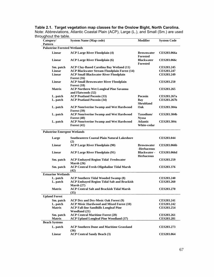
67
Table 2.1. Target vegetation map classes for the Onslow Bight, North Carolina. Note: Abbreviations, Atlantic Coastal Plain (ACP), Large (L.), and Small (Sm.) are used throughout the table.
Category/ Pattern
System Name (Map code) Modifier System Code
Palustrine Forested Wetlands Linear ACP Large River Floodplain (4) Brownwater
Forested CES203.066a
Linear ACP Large River Floodplain (6) Blackwater Forested
CES203.066c
Sm. patch ACP Clay-Based Carolina Bay Wetland (11) CES203.245 Linear ACP Blackwater Stream Floodplain Forest (14) CES203.247 Linear ACP Small Blackwater River Floodplain
Forest (16) CES203.249
Linear ACP Small Brownwater River Floodplain Forest (18)
CES203.250
Matrix ACP Northern Wet Longleaf Pine Savanna and Flatwoods (32)
CES203.265
L. patch ACP Peatland Pocosin (33) Pocosin CES203.267a L. patch ACP Peatland Pocosin (34) Bay
Shrubland CES203.267b
L. patch ACP Nonriverine Swamp and Wet Hardwood Forest (39)
Oak CES203.304a
L. patch ACP Nonriverine Swamp and Wet Hardwood Forest (40)
Taxodium/ Nyssa
CES203.304b
L. patch ACP Nonriverine Swamp and Wet Hardwood Forest (41)
Atlantic White-cedar
CES203.304c
Palustrine Emergent Wetlands
Large Southeastern Coastal Plain Natural Lakeshore (2)
CES203.044
Linear ACP Large River Floodplain (90) Brownwater -Herbaceous
CES203.066b
Linear ACP Large River Floodplain (91) Blackwater - Herbaceous
CES203.066d
Sm. patch ACP Embayed Region Tidal Freshwater Marsh (26)
CES203.259
Sm. patch ACP Central Fresh-Oligohaline Tidal Marsh (42)
CES203.376
Estuarine Wetlands L. patch ACP Southern Tidal Wooded Swamp (8) CES203.240 L. patch ACP Embayed Region Tidal Salt and Brackish
Marsh (27) CES203.260
Matrix ACP Central Salt and Brackish Tidal Marsh (35)
CES203.270
Upland Forest Sm. patch ACP Dry and Dry-Mesic Oak Forest (9) CES203.241 L. patch ACP Mesic Hardwood and Mixed Forest (10) CES203.242 Matrix ACP Fall-line Sandhills Longleaf Pine
Woodland (21) CES203.254
Sm. patch ACP Central Maritime Forest (28) CES203.261 Matrix ACP Upland Longleaf Pine Woodland (37) CES203.281
Beach Systems L. patch ACP Southern Dune and Maritime Grassland
(36) CES203.273
Linear ACP Central Sandy Beach (3) CES203.064
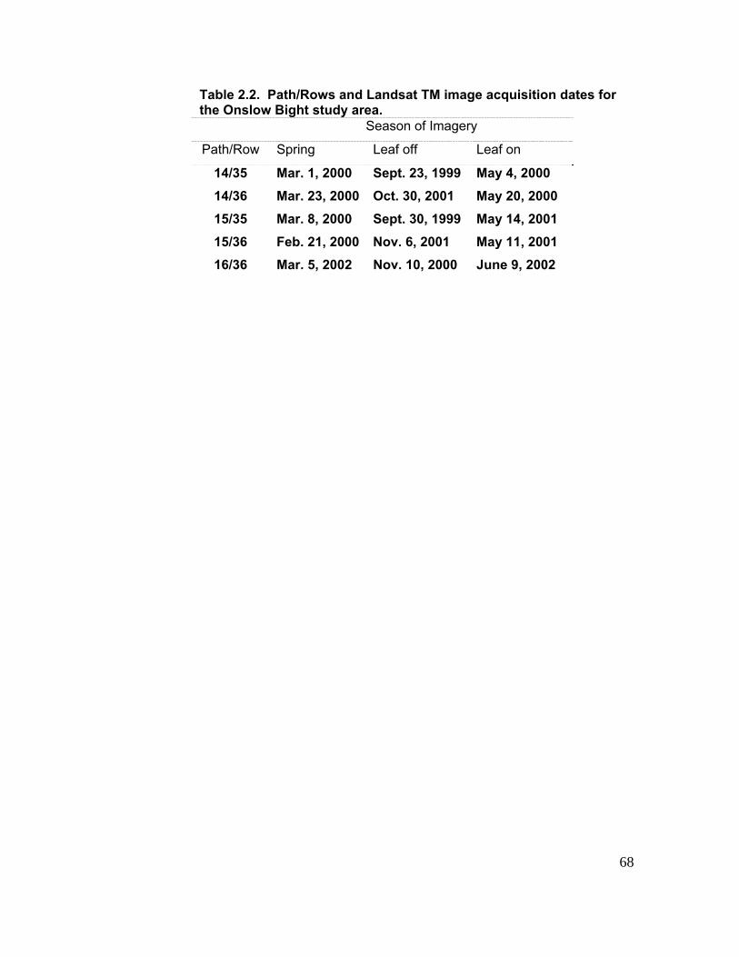
68
Table 2.2. Path/Rows and Landsat TM image acquisition dates for the Onslow Bight study area.
Season of Imagery
Path/Row Spring Leaf off Leaf on
14/35 Mar. 1, 2000 Sept. 23, 1999 May 4, 2000 14/36 Mar. 23, 2000 Oct. 30, 2001 May 20, 2000 15/35 Mar. 8, 2000 Sept. 30, 1999 May 14, 2001 15/36 Feb. 21, 2000 Nov. 6, 2001 May 11, 2001 16/36 Mar. 5, 2002 Nov. 10, 2000 June 9, 2002

69
Table 2.3. Wetland map classes included in Zone 58 in addition to the NLCD 2001 legend. NLCD Level II Class Zone 58 Class
Forested Wetland Palustrine Deciduous Forested Wetland Palustrine Evergreen Forested Wetland Palustrine Scrub/Shrub Wetland Estuarine Forested Wetland Estuarine Scrub/Shrub Wetland
Emergent Wetland Palustrine Emergent Wetland
Estuarine Emergent Wetland
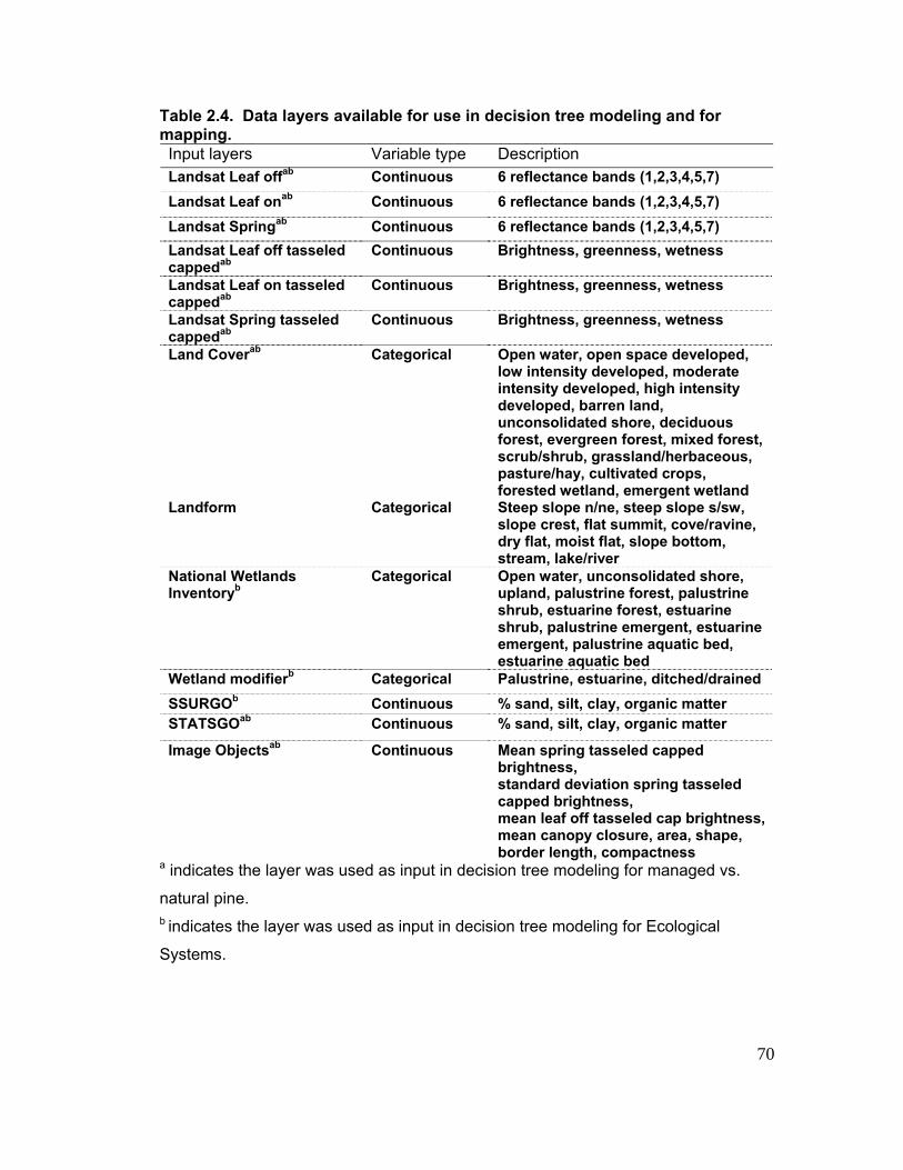
70
Table 2.4. Data layers available for use in decision tree modeling and for mapping. Input layers Variable type Description Landsat Leaf offab Continuous 6 reflectance bands (1,2,3,4,5,7) Landsat Leaf onab Continuous 6 reflectance bands (1,2,3,4,5,7) Landsat Springab Continuous 6 reflectance bands (1,2,3,4,5,7) Landsat Leaf off tasseled cappedab
Continuous Brightness, greenness, wetness
Landsat Leaf on tasseled cappedab
Continuous Brightness, greenness, wetness
Landsat Spring tasseled cappedab
Continuous Brightness, greenness, wetness
Land Coverab Categorical Open water, open space developed, low intensity developed, moderate intensity developed, high intensity developed, barren land, unconsolidated shore, deciduous forest, evergreen forest, mixed forest, scrub/shrub, grassland/herbaceous, pasture/hay, cultivated crops, forested wetland, emergent wetland
Landform Categorical Steep slope n/ne, steep slope s/sw, slope crest, flat summit, cove/ravine, dry flat, moist flat, slope bottom, stream, lake/river
National Wetlands Inventoryb
Categorical Open water, unconsolidated shore, upland, palustrine forest, palustrine shrub, estuarine forest, estuarine shrub, palustrine emergent, estuarine emergent, palustrine aquatic bed, estuarine aquatic bed
Wetland modifierb Categorical Palustrine, estuarine, ditched/drained SSURGOb Continuous % sand, silt, clay, organic matter STATSGOab Continuous % sand, silt, clay, organic matter
Image Objectsab Continuous Mean spring tasseled capped brightness, standard deviation spring tasseled capped brightness, mean leaf off tasseled cap brightness, mean canopy closure, area, shape, border length, compactness
a indicates the layer was used as input in decision tree modeling for managed vs.
natural pine.
b indicates the layer was used as input in decision tree modeling for Ecological
Systems.
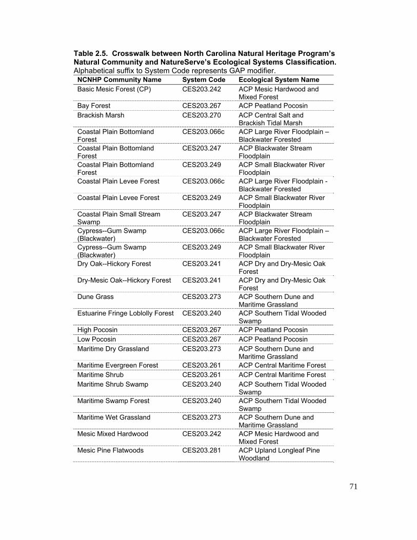
71
Table 2.5. Crosswalk between North Carolina Natural Heritage Program’s Natural Community and NatureServe’s Ecological Systems Classification. Alphabetical suffix to System Code represents GAP modifier. NCNHP Community Name System Code Ecological System Name Basic Mesic Forest (CP) CES203.242 ACP Mesic Hardwood and
Mixed Forest Bay Forest CES203.267 ACP Peatland Pocosin Brackish Marsh CES203.270 ACP Central Salt and
Brackish Tidal Marsh Coastal Plain Bottomland Forest
CES203.066c ACP Large River Floodplain – Blackwater Forested
Coastal Plain Bottomland Forest
CES203.247 ACP Blackwater Stream Floodplain
Coastal Plain Bottomland Forest
CES203.249 ACP Small Blackwater River Floodplain
Coastal Plain Levee Forest CES203.066c ACP Large River Floodplain - Blackwater Forested
Coastal Plain Levee Forest CES203.249 ACP Small Blackwater River Floodplain
Coastal Plain Small Stream Swamp
CES203.247 ACP Blackwater Stream Floodplain
Cypress--Gum Swamp (Blackwater)
CES203.066c ACP Large River Floodplain – Blackwater Forested
Cypress--Gum Swamp (Blackwater)
CES203.249 ACP Small Blackwater River Floodplain
Dry Oak--Hickory Forest CES203.241 ACP Dry and Dry-Mesic Oak Forest
Dry-Mesic Oak--Hickory Forest CES203.241 ACP Dry and Dry-Mesic Oak Forest
Dune Grass CES203.273 ACP Southern Dune and Maritime Grassland
Estuarine Fringe Loblolly Forest CES203.240 ACP Southern Tidal Wooded Swamp
High Pocosin CES203.267 ACP Peatland Pocosin Low Pocosin CES203.267 ACP Peatland Pocosin Maritime Dry Grassland CES203.273 ACP Southern Dune and
Maritime Grassland Maritime Evergreen Forest CES203.261 ACP Central Maritime Forest Maritime Shrub CES203.261 ACP Central Maritime Forest Maritime Shrub Swamp CES203.240 ACP Southern Tidal Wooded
Swamp Maritime Swamp Forest CES203.240 ACP Southern Tidal Wooded
Swamp Maritime Wet Grassland CES203.273 ACP Southern Dune and
Maritime Grassland Mesic Mixed Hardwood CES203.242 ACP Mesic Hardwood and
Mixed Forest Mesic Pine Flatwoods CES203.281 ACP Upland Longleaf Pine
Woodland
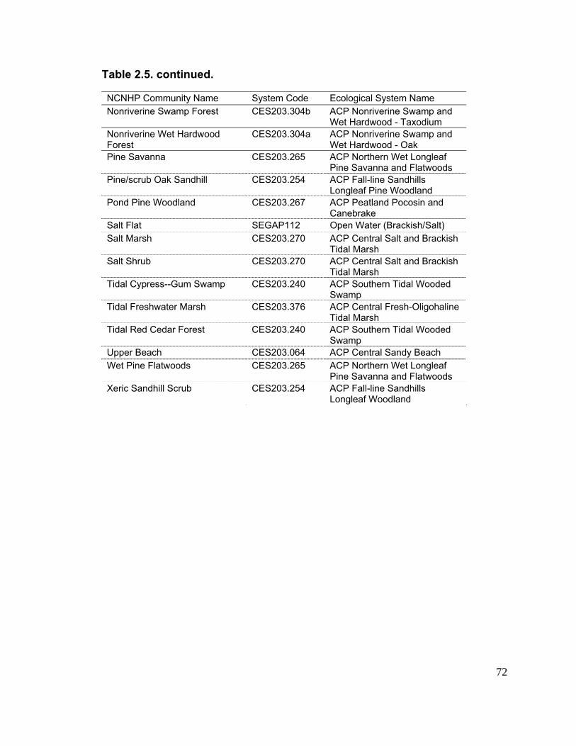
72
Table 2.5. continued. NCNHP Community Name System Code Ecological System Name Nonriverine Swamp Forest CES203.304b ACP Nonriverine Swamp and
Wet Hardwood - Taxodium Nonriverine Wet Hardwood Forest
CES203.304a ACP Nonriverine Swamp and Wet Hardwood - Oak
Pine Savanna CES203.265 ACP Northern Wet Longleaf Pine Savanna and Flatwoods
Pine/scrub Oak Sandhill CES203.254 ACP Fall-line Sandhills Longleaf Pine Woodland
Pond Pine Woodland CES203.267 ACP Peatland Pocosin and Canebrake
Salt Flat SEGAP112 Open Water (Brackish/Salt) Salt Marsh CES203.270 ACP Central Salt and Brackish
Tidal Marsh Salt Shrub CES203.270 ACP Central Salt and Brackish
Tidal Marsh Tidal Cypress--Gum Swamp CES203.240 ACP Southern Tidal Wooded
Swamp Tidal Freshwater Marsh CES203.376 ACP Central Fresh-Oligohaline
Tidal Marsh Tidal Red Cedar Forest CES203.240 ACP Southern Tidal Wooded
Swamp Upper Beach CES203.064 ACP Central Sandy Beach Wet Pine Flatwoods CES203.265 ACP Northern Wet Longleaf
Pine Savanna and Flatwoods Xeric Sandhill Scrub CES203.254 ACP Fall-line Sandhills
Longleaf Woodland
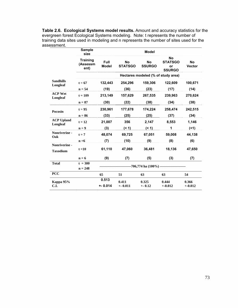
73
Table 2.6. Ecological Systems model results. Amount and accuracy statistics for the evergreen forest Ecological Systems modeling. Note: t represents the number of training data sites used in modeling and n represents the number of sites used for the assessment.
Sample size Model
Training (Assessm
ent) Full
Model No
STATSGO No
SSURGO
No STATSGO
or SSURGO
No Vector
Hectares modeled (% of study area) Sandhills Longleaf t = 67 132,443 254,296 159,306 122,609 100,671
n = 54 (19) (36) (23) (17) (14) ACP Wet Longleaf t = 109 213,149 157,629 267,535 239,963 270,624
n = 87 (30) (22) (38) (34) (38)
Pocosin t = 95 230,961 177,678 174,224 258,474 242,515
n = 86 (33) (25) (25) (37) (34) ACP Upland Longleaf t = 12 21,007 356 2,147 8,553 1,146
n = 9 (3) (< 1) (< 1) 1 (<1) Nonriverine - Oak t = 7 48,074 69,725 67,051 59,008 44,138
n =6 (7) (10) (9) (8) (6) Nonriverine -
Taxodium t =10 61,110 47,060 36,481 18,136 47,650
n = 6 (9) (7) (5) (3) (7) Total t = 300
n = 248 ---------------------------706,774 ha (100%) ----------------------
PCC 65 51 63 63 54
Kappa 95% C.I.
0.513
+- 0.014 0.411 +- 0.011
0.325 +- 0.12
0.444 +-0.012
0.366 +-0.012
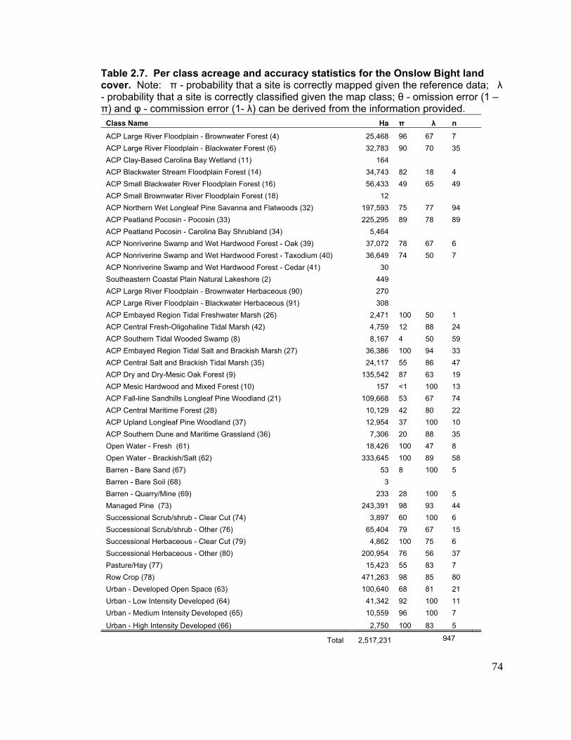
74
Table 2.7. Per class acreage and accuracy statistics for the Onslow Bight land cover. Note: π - probability that a site is correctly mapped given the reference data; λ - probability that a site is correctly classified given the map class; θ - omission error (1 – π) and φ - commission error (1- λ) can be derived from the information provided.
Class Name Ha π λ n
ACP Large River Floodplain - Brownwater Forest (4) 25,468 96 67 7 ACP Large River Floodplain - Blackwater Forest (6) 32,783 90 70 35 ACP Clay-Based Carolina Bay Wetland (11) 164 ACP Blackwater Stream Floodplain Forest (14) 34,743 82 18 4 ACP Small Blackwater River Floodplain Forest (16) 56,433 49 65 49 ACP Small Brownwater River Floodplain Forest (18) 12 ACP Northern Wet Longleaf Pine Savanna and Flatwoods (32) 197,593 75 77 94 ACP Peatland Pocosin - Pocosin (33) 225,295 89 78 89 ACP Peatland Pocosin - Carolina Bay Shrubland (34) 5,464 ACP Nonriverine Swamp and Wet Hardwood Forest - Oak (39) 37,072 78 67 6 ACP Nonriverine Swamp and Wet Hardwood Forest - Taxodium (40) 36,649 74 50 7 ACP Nonriverine Swamp and Wet Hardwood Forest - Cedar (41) 30 Southeastern Coastal Plain Natural Lakeshore (2) 449 ACP Large River Floodplain - Brownwater Herbaceous (90) 270 ACP Large River Floodplain - Blackwater Herbaceous (91) 308 ACP Embayed Region Tidal Freshwater Marsh (26) 2,471 100 50 1 ACP Central Fresh-Oligohaline Tidal Marsh (42) 4,759 12 88 24 ACP Southern Tidal Wooded Swamp (8) 8,167 4 50 59 ACP Embayed Region Tidal Salt and Brackish Marsh (27) 36,386 100 94 33 ACP Central Salt and Brackish Tidal Marsh (35) 24,117 55 86 47 ACP Dry and Dry-Mesic Oak Forest (9) 135,542 87 63 19 ACP Mesic Hardwood and Mixed Forest (10) 157 <1 100 13 ACP Fall-line Sandhills Longleaf Pine Woodland (21) 109,668 53 67 74 ACP Central Maritime Forest (28) 10,129 42 80 22 ACP Upland Longleaf Pine Woodland (37) 12,954 37 100 10 ACP Southern Dune and Maritime Grassland (36) 7,306 20 88 35 Open Water - Fresh (61) 18,426 100 47 8 Open Water - Brackish/Salt (62) 333,645 100 89 58 Barren - Bare Sand (67) 53 8 100 5 Barren - Bare Soil (68) 3 Barren - Quarry/Mine (69) 233 28 100 5 Managed Pine (73) 243,391 98 93 44 Successional Scrub/shrub - Clear Cut (74) 3,897 60 100 6 Successional Scrub/shrub - Other (76) 65,404 79 67 15 Successional Herbaceous - Clear Cut (79) 4,862 100 75 6 Successional Herbaceous - Other (80) 200,954 76 56 37 Pasture/Hay (77) 15,423 55 83 7 Row Crop (78) 471,263 98 85 80 Urban - Developed Open Space (63) 100,640 68 81 21 Urban - Low Intensity Developed (64) 41,342 92 100 11 Urban - Medium Intensity Developed (65) 10,559 96 100 7
Urban - High Intensity Developed (66) 2,750 100 83 5
Total 2,517,231 947
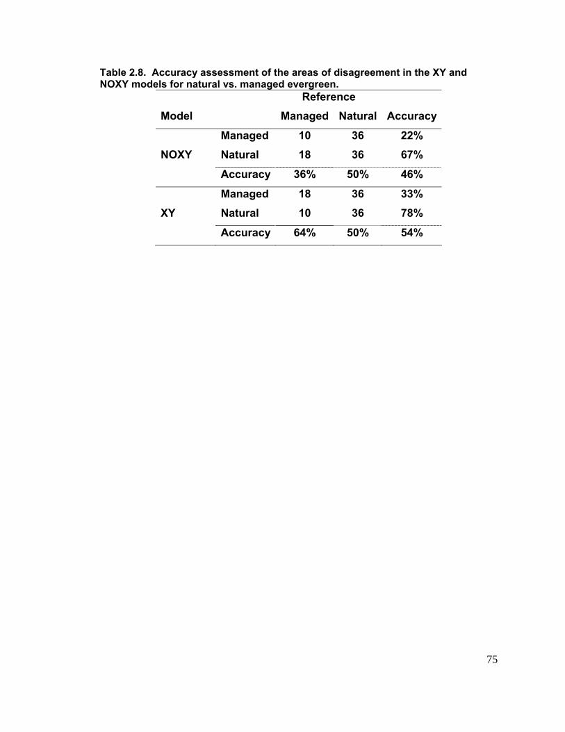
75
Table 2.8. Accuracy assessment of the areas of disagreement in the XY and NOXY models for natural vs. managed evergreen.
Reference Model Managed Natural Accuracy
Managed 10 36 22% NOXY Natural 18 36 67%
Accuracy 36% 50% 46%
Managed 18 36 33% XY Natural 10 36 78%
Accuracy 64% 50% 54%
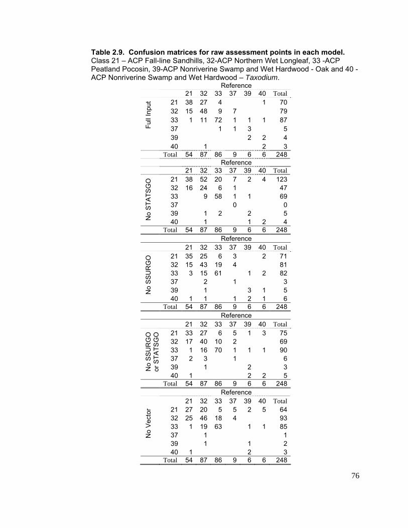
76
Table 2.9. Confusion matrices for raw assessment points in each model. Class 21 – ACP Fall-line Sandhills, 32-ACP Northern Wet Longleaf, 33 -ACP Peatland Pocosin, 39-ACP Nonriverine Swamp and Wet Hardwood - Oak and 40 - ACP Nonriverine Swamp and Wet Hardwood – Taxodium.
Reference 21 32 33 37 39 40 Total
21 38 27 4 1 70 32 15 48 9 7 79 33 1 11 72 1 1 1 87 37 1 1 3 5 39 2 2 4
Ful
l Inp
ut
40 1 2 3 Total 54 87 86 9 6 6 248 Reference 21 32 33 37 39 40 Total
21 38 52 20 7 2 4 123 32 16 24 6 1 47 33 9 58 1 1 69 37 0 0 39 1 2 2 5
No
STA
TSG
O
40 1 1 2 4 Total 54 87 86 9 6 6 248 Reference 21 32 33 37 39 40 Total
21 35 25 6 3 2 71 32 15 43 19 4 81 33 3 15 61 1 2 82 37 2 1 3 39 1 3 1 5 N
o S
SU
RG
O
40 1 1 1 2 1 6 Total 54 87 86 9 6 6 248 Reference 21 32 33 37 39 40 Total
21 33 27 6 5 1 3 75 32 17 40 10 2 69 33 1 16 70 1 1 1 90 37 2 3 1 6 39 1 2 3 N
o S
SU
RG
O
or S
TATS
GO
40 1 2 2 5 Total 54 87 86 9 6 6 248 Reference
21 32 33 37 39 40 Total 21 27 20 5 5 2 5 64 32 25 46 18 4 93 33 1 19 63 1 1 85 37 1 1 39 1 1 2
No
Vec
tor
40 1 2 3 Total 54 87 86 9 6 6 248
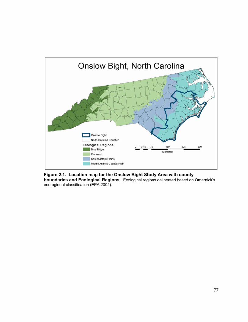
Figure 2.1. Location map for the Onslow Bight Study Area with county boundaries and Ecological Regions. Ecological regions delineated based on Omernick’s ecoregional classification (EPA 2004).
77
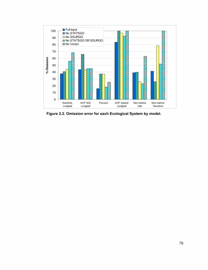
0
10
20
30
40
50
60
70
80
90
100
SandhillsLongleaf
ACP WetLongleaf
Pocosin ACP UplandLongleaf
Non-riverineOak
Non-riverineTaxodium
% O
mis
sion
Full InputNo STATSGONo SSURGONo STATSGO OR SSURGONo Vector
Figure 2.2. Omission error for each Ecological System by model.
78
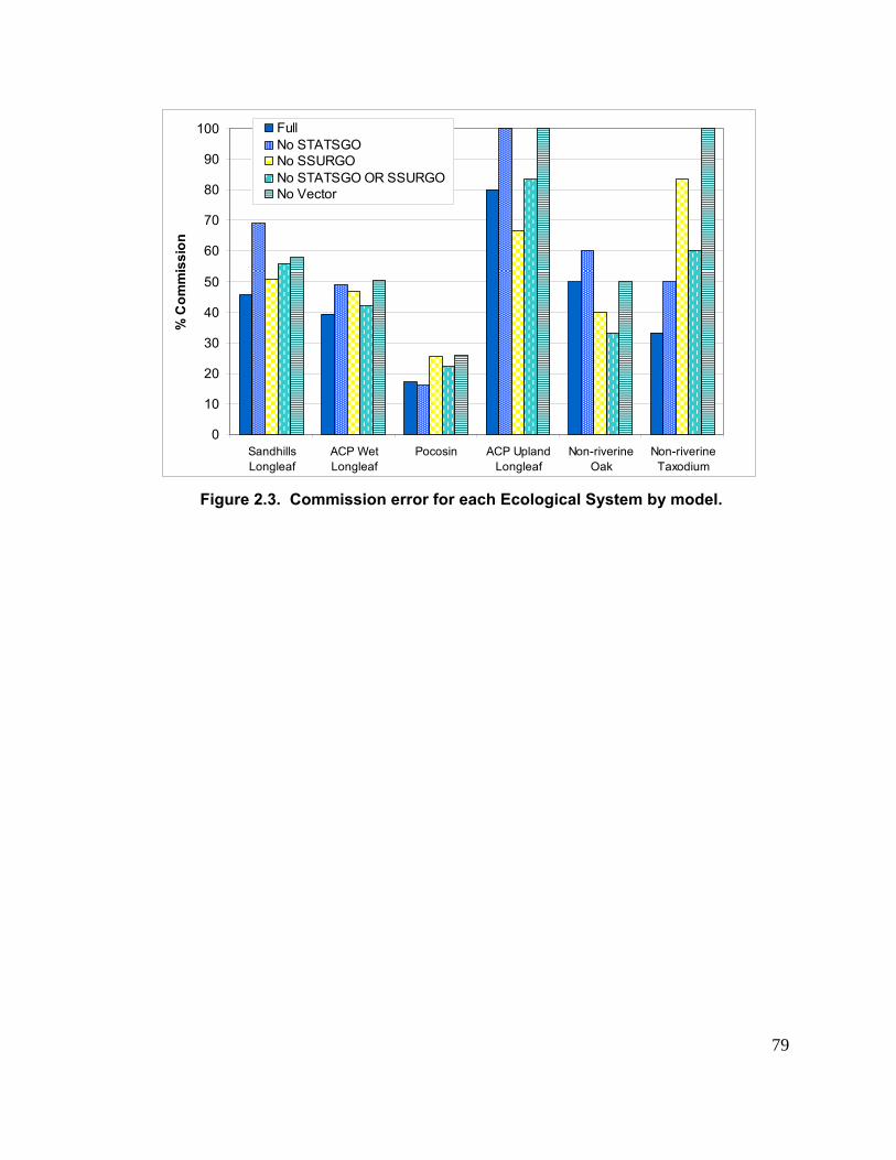
0
10
20
30
40
50
60
70
80
90
100
SandhillsLongleaf
ACP WetLongleaf
Pocosin ACP UplandLongleaf
Non-riverineOak
Non-riverineTaxodium
% C
omm
issi
on
FullNo STATSGONo SSURGONo STATSGO OR SSURGONo Vector
Figure 2.3. Commission error for each Ecological System by model.
79
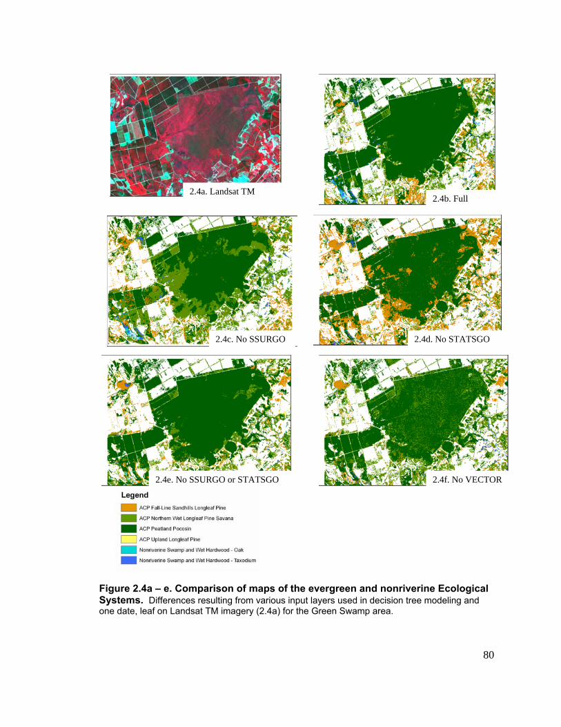
80
igure 2.4a – e. Comparison of maps of the evergreen and nonriverine Ecological ystems. Differences resulting from various input layers used in decision tree modeling and ne date, leaf on Landsat TM imagery (2.4a) for the Green Swamp area.
2.4a. Landsat TM 2.4b. Full
2.4c. No SSURGO 2.4d. No STATSGO
2.4e. No SSURGO or STATSGO 2.4f. No VECTOR
FSo
81
age objects and change vector analysis for monitoring changes in the plant ommunities in the Onslow Bight, North Carolina.
lexa J. McKerrow1, Heather M. Cheshire2, and Thomas R. Wentworth3
Gap Analysis Project, Department of Zoology, North Carolina State
h Carolina State University 27695-7612 ([email protected]) Abstract Effective conservation planning requires information on both the content and context for
the resources to be conserved. Land cover mapping and change detection are one set
of tools that provide both the content (spatially explicit land cover) and the context (land
cover changes). Our goal was to develop an approach to change detection that could
be used with a thematically rich land cover map. We used the 2001 Ecological Systems
map developed by the Southeast Gap Analysis Project as our baseline dataset. Our
study area was the Onslow Bight in the Middle Atlantic Coastal Plain of North Carolina.
The method combined Change Vector Analysis (CVA), image segmentation (image
objects), and regression tree modeling to back cast to a 1992 era land cover map. The
overall accuracy based on marginal frequencies was 95% with a Kappa of 0.78. There
was a 21% probability that a point that did not change was misclassified as one that had
changed, and a 17% probability that a change was missed. Thirteen percent of the
study area was mapped as having changed. Most of the land cover changes were
between anthropogenic land cover types, but the approach provided the context
necessary to map the changes in the Ecological Systems of the Onslow Bight. Using
this approach we were able to accurately map change in a complex landscape and to
avoid a common mistake of over-mapping change in the agricultural classes. In future
work we hope to find methods for automating portions of the process, specifically: (1)
setting the initial change thresholds based on the magnitude of change between image
dates; and (2) classifying the class-specific types of change.
Keywords: Change Detection, Change Vector Analysis, Image Objects, Ecological Systems, Gap Analysis Program.
Imc A
1 Southeast University, Raleigh, NC 27695-7617 ([email protected]); 2 Department of Forestry and Natural Resources, North Carolina State University 27695-8808 ([email protected]); 3 Department of Plant Biology, Nort
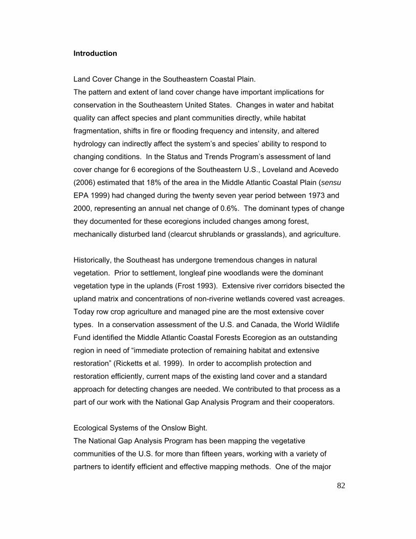
82
The pattern and extent of land cover change have important implications for
ydrology can indirectly affect the system’s and species’ ability to respond to
onditions. In the Status and Trends Program’s assessment of land
cological Systems of the Onslow Bight.
han fifteen years, working with a variety of
artners to identify efficient and effective mapping methods. One of the major
Introduction Land Cover Change in the Southeastern Coastal Plain.
conservation in the Southeastern United States. Changes in water and habitat
quality can affect species and plant communities directly, while habitat
fragmentation, shifts in fire or flooding frequency and intensity, and altered
h
changing c
cover change for 6 ecoregions of the Southeastern U.S., Loveland and Acevedo
(2006) estimated that 18% of the area in the Middle Atlantic Coastal Plain (sensu
EPA 1999) had changed during the twenty seven year period between 1973 and
2000, representing an annual net change of 0.6%. The dominant types of change
they documented for these ecoregions included changes among forest,
mechanically disturbed land (clearcut shrublands or grasslands), and agriculture.
Historically, the Southeast has undergone tremendous changes in natural
vegetation. Prior to settlement, longleaf pine woodlands were the dominant
vegetation type in the uplands (Frost 1993). Extensive river corridors bisected the
upland matrix and concentrations of non-riverine wetlands covered vast acreages.
Today row crop agriculture and managed pine are the most extensive cover
types. In a conservation assessment of the U.S. and Canada, the World Wildlife
Fund identified the Middle Atlantic Coastal Forests Ecoregion as an outstanding
region in need of “immediate protection of remaining habitat and extensive
restoration” (Ricketts et al. 1999). In order to accomplish protection and
restoration efficiently, current maps of the existing land cover and a standard
approach for detecting changes are needed. We contributed to that process as a
part of our work with the National Gap Analysis Program and their cooperators.
E
The National Gap Analysis Program has been mapping the vegetative
ommunities of the U.S. for more tc
p
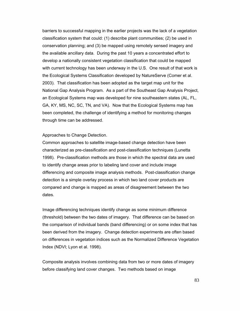
83
cessful mapping in the earlier projects was the lack of a vegetation
lassification system that could: (1) describe plant communities; (2) be used in
ly sensed imagery and
at work is
al.
ct,
ommon approaches to satellite image-based change detection have been
tta
ed
ce
n
n differences in vegetation indices such as the Normalized Difference Vegetation
ry
barriers to suc
c
conservation planning; and (3) be mapped using remote
the available ancillary data. During the past 10 years a concentrated effort to
develop a nationally consistent vegetation classification that could be mapped
with current technology has been underway in the U.S. One result of th
the Ecological Systems Classification developed by NatureServe (Comer et
2003). That classification has been adopted as the target map unit for the
National Gap Analysis Program. As a part of the Southeast Gap Analysis Proje
an Ecological Systems map was developed for nine southeastern states (AL, FL,
GA, KY, MS, NC, SC, TN, and VA). Now that the Ecological Systems map has
been completed, the challenge of identifying a method for monitoring changes
through time can be addressed.
Approaches to Change Detection.
C
characterized as pre-classification and post-classification techniques (Lune
1998). Pre-classification methods are those in which the spectral data are us
to identify change areas prior to labeling land cover and include image
differencing and composite image analysis methods. Post-classification change
detection is a simple overlay process in which two land cover products are
compared and change is mapped as areas of disagreement between the two
dates.
Image differencing techniques identify change as some minimum differen
(threshold) between the two dates of imagery. That difference can be based o
the comparison of individual bands (band differencing) or on some index that has
been derived from the imagery. Change detection experiments are often based
o
Index (NDVI; Lyon et al. 1998).
Composite analysis involves combining data from two or more dates of image
before classifying land cover changes. Two methods based on image
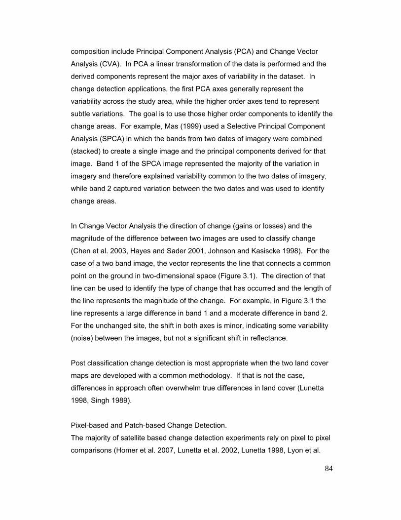
84
ned
e (gains or losses) and the
he
n of that
f
the
2.
unchanged site, the shift in both axes is minor, indicating some variability
oise) between the images, but not a significant shift in reflectance.
ixel-based and Patch-based Change Detection.
l
n et al.
composition include Principal Component Analysis (PCA) and Change Vector
Analysis (CVA). In PCA a linear transformation of the data is performed and the
derived components represent the major axes of variability in the dataset. In
change detection applications, the first PCA axes generally represent the
variability across the study area, while the higher order axes tend to represent
subtle variations. The goal is to use those higher order components to identify the
change areas. For example, Mas (1999) used a Selective Principal Component
Analysis (SPCA) in which the bands from two dates of imagery were combi
(stacked) to create a single image and the principal components derived for that
image. Band 1 of the SPCA image represented the majority of the variation in
imagery and therefore explained variability common to the two dates of imagery,
while band 2 captured variation between the two dates and was used to identify
change areas.
In Change Vector Analysis the direction of chang
magnitude of the difference between two images are used to classify change
(Chen et al. 2003, Hayes and Sader 2001, Johnson and Kasiscke 1998). For t
case of a two band image, the vector represents the line that connects a common
point on the ground in two-dimensional space (Figure 3.1). The directio
line can be used to identify the type of change that has occurred and the length o
the line represents the magnitude of the change. For example, in Figure 3.1
line represents a large difference in band 1 and a moderate difference in band
For the
(n
Post classification change detection is most appropriate when the two land cover
maps are developed with a common methodology. If that is not the case,
differences in approach often overwhelm true differences in land cover (Lunetta
1998, Singh 1989).
P
The majority of satellite based change detection experiments rely on pixel to pixe
comparisons (Homer et al. 2007, Lunetta et al. 2002, Lunetta 1998, Lyo
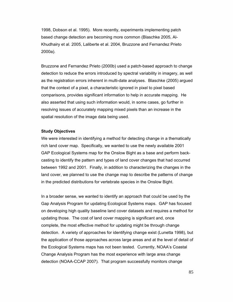
85
l
d
of the image data being used.
lly
sed by the
ap Analysis Program for updating Ecological Systems maps. GAP has focused
of approaches for identifying change exist (Lunetta 1998), but
e application of those approaches across large areas and at the level of detail of
. Currently, NOAA’s Coastal
1998, Dobson et al. 1995). More recently, experiments implementing patch
based change detection are becoming more common (Blaschke 2005, Al-
Khudhairy et al. 2005, Laliberte et al. 2004, Bruzzone and Fernandez Prieto
2000a).
Bruzzone and Fernandez Prieto (2000b) used a patch-based approach to change
detection to reduce the errors introduced by spectral variability in imagery, as wel
as the registration errors inherent in multi-date analyses. Blaschke (2005) argue
that the context of a pixel, a characteristic ignored in pixel to pixel based
comparisons, provides significant information to help in accurate mapping. He
also asserted that using such information would, in some cases, go further in
resolving issues of accurately mapping mixed pixels than an increase in the
spatial resolution
Study Objectives We were interested in identifying a method for detecting change in a thematica
rich land cover map. Specifically, we wanted to use the newly available 2001
GAP Ecological Systems map for the Onslow Bight as a base and perform back-
casting to identify the pattern and types of land cover changes that had occurred
between 1992 and 2001. Finally, in addition to characterizing the changes in the
land cover, we planned to use the change map to describe the patterns of change
in the predicted distributions for vertebrate species in the Onslow Bight.
In a broader sense, we wanted to identify an approach that could be u
G
on developing high quality baseline land cover datasets and requires a method for
updating those. The cost of land cover mapping is significant and, once
complete, the most effective method for updating might be through change
detection. A variety
th
the Ecological Systems maps has not been tested
Change Analysis Program has the most experience with large area change
detection (NOAA-CCAP 2007). That program successfully monitors change
86
is
cently
CD
Homer et al. 2007). That effort will determine change between 6
eneral land cover classes in order to rapidly assess change for the coterminous
t
of
ur study area, the Onslow Bight, covers more than 250,000 km2 of land in the
rth Carolina. The area supports a diverse set of natural plant
d by
pen (salt and brackish) water. The Atlantic Coastal Plain Peatland Pocosin is
ing
between 28 land cover classes. The land cover classification used by CCAP
based on vegetation structure, hydrology, and physiognomy. USGS has re
initiated an effort to detect change nationally, based on the 1992 and 2001 NL
datasets (
g
U.S. Future plans include developing protocols for detecting change among the
21 land cover classes of the NLCD 2001. Again, that classification is based on
vegetation structure, hydrology, and physiognomy, and does not include a
species composition component. In this study we planned to perform tha
evaluation and, if successful, identify an effective approach to meeting the goal
efficient updating for GAP’s land cover maps.
Study Area O
Coastal Plain of No
communities including maritime forests, coastal marshes, pocosins, and longleaf
pine woodlands (Figure 3.2). The area was first settled in the early 1700s.
Currently, coastal development, forest management, and farming are the
dominant land uses in the region. Lands in public management represent 5% of
the area, with Department of Defense, U.S. Fish and Wildlife Service, and the N.
C. Wildlife Resources Commission managing the majority of those lands. The
most extensive land cover in the study area is row crop agriculture, followe
o
the most extensive Ecological System in the present landscape (Figure 3.2).
Methods There were three major steps in our change detection process.
1. Pre-processing the imagery, determining the change vectors, and identify
the potential change areas (Figure 3.3);
2. Labeling change for the Non-Urban land cover classes (Figure 3.4); and
3. Labeling change for the Urban areas (Figure 3.5).
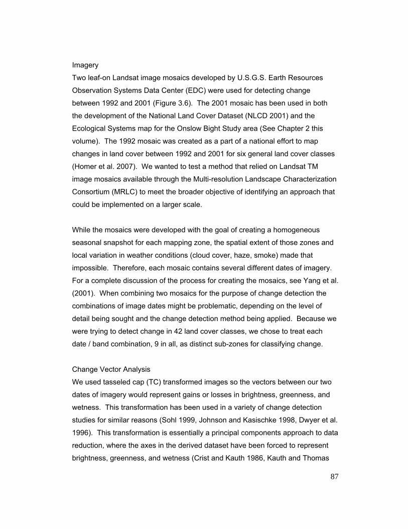
87
asses
lution Landscape Characterization
onsortium (MRLC) to meet the broader objective of identifying an approach that
emented on a larger scale.
agery.
.
e
ctor Analysis
tween our two
sed in a variety of change detection
r et al.
omponents approach to data
duction, where the axes in the derived dataset have been forced to represent
brightness, greenness, and wetness (Crist and Kauth 1986, Kauth and Thomas
Imagery
Two leaf-on Landsat image mosaics developed by U.S.G.S. Earth Resources
Observation Systems Data Center (EDC) were used for detecting change
between 1992 and 2001 (Figure 3.6). The 2001 mosaic has been used in both
the development of the National Land Cover Dataset (NLCD 2001) and the
Ecological Systems map for the Onslow Bight Study area (See Chapter 2 this
volume). The 1992 mosaic was created as a part of a national effort to map
changes in land cover between 1992 and 2001 for six general land cover cl
(Homer et al. 2007). We wanted to test a method that relied on Landsat TM
image mosaics available through the Multi-reso
C
could be impl
While the mosaics were developed with the goal of creating a homogeneous
seasonal snapshot for each mapping zone, the spatial extent of those zones and
local variation in weather conditions (cloud cover, haze, smoke) made that
impossible. Therefore, each mosaic contains several different dates of im
For a complete discussion of the process for creating the mosaics, see Yang et al
(2001). When combining two mosaics for the purpose of change detection the
combinations of image dates might be problematic, depending on the level of
detail being sought and the change detection method being applied. Because w
were trying to detect change in 42 land cover classes, we chose to treat each
date / band combination, 9 in all, as distinct sub-zones for classifying change.
Change Ve
We used tasseled cap (TC) transformed images so the vectors be
dates of imagery would represent gains or losses in brightness, greenness, and
wetness. This transformation has been u
studies for similar reasons (Sohl 1999, Johnson and Kasischke 1998, Dwye
1996). This transformation is essentially a principal c
re
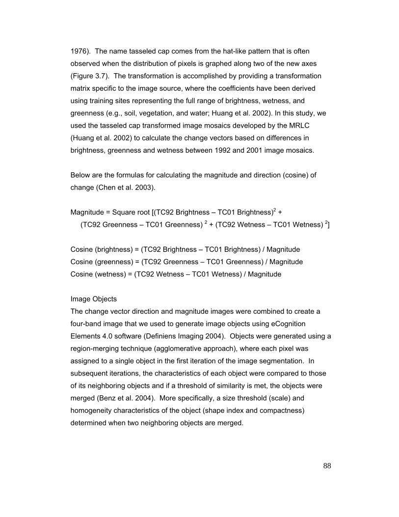
88
976). The name tasseled cap comes from the hat-like pattern that is often
when the distribution of pixels is graphed along two of the new axes
ed
, we
agnitude = Square root [(TC92 Brightness – TC01 Brightness)2 +
s) 2]
g a
gion-merging technique (agglomerative approach), where each pixel was
t in the first iteration of the image segmentation. In
1
observed
(Figure 3.7). The transformation is accomplished by providing a transformation
matrix specific to the image source, where the coefficients have been deriv
using training sites representing the full range of brightness, wetness, and
greenness (e.g., soil, vegetation, and water; Huang et al. 2002). In this study
used the tasseled cap transformed image mosaics developed by the MRLC
(Huang et al. 2002) to calculate the change vectors based on differences in
brightness, greenness and wetness between 1992 and 2001 image mosaics.
Below are the formulas for calculating the magnitude and direction (cosine) of
change (Chen et al. 2003).
M
(TC92 Greenness – TC01 Greenness) 2 + (TC92 Wetness – TC01 Wetnes
Cosine (brightness) = (TC92 Brightness – TC01 Brightness) / Magnitude
Cosine (greenness) = (TC92 Greenness – TC01 Greenness) / Magnitude
Cosine (wetness) = (TC92 Wetness – TC01 Wetness) / Magnitude
Image Objects
The change vector direction and magnitude images were combined to create a
four-band image that we used to generate image objects using eCognition
Elements 4.0 software (Definiens Imaging 2004). Objects were generated usin
re
assigned to a single objec
subsequent iterations, the characteristics of each object were compared to those
of its neighboring objects and if a threshold of similarity is met, the objects were
merged (Benz et al. 2004). More specifically, a size threshold (scale) and
homogeneity characteristics of the object (shape index and compactness)
determined when two neighboring objects are merged.
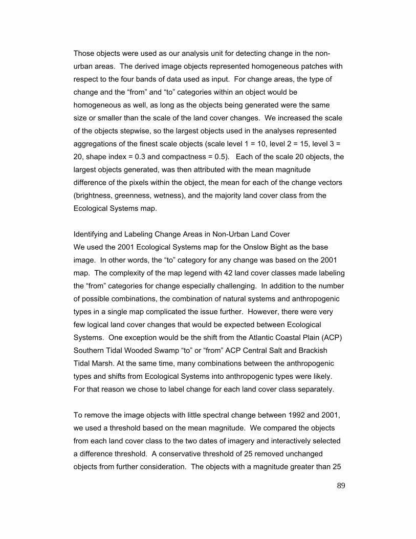
89
-
ith
e
ted
l 3 =
he
rgest objects generated, was then attributed with the mean magnitude
rs
ness), and the majority land cover class from the
cological Systems map.
e used the 2001 Ecological Systems map for the Onslow Bight as the base
2001
beling
to the number
f possible combinations, the combination of natural systems and anthropogenic
map complicated the issue further. However, there were very
ACP)
ic
2001,
ects
nd interactively selected
difference threshold. A conservative threshold of 25 removed unchanged
objects from further consideration. The objects with a magnitude greater than 25
Those objects were used as our analysis unit for detecting change in the non
urban areas. The derived image objects represented homogeneous patches w
respect to the four bands of data used as input. For change areas, the type of
change and the “from” and “to” categories within an object would be
homogeneous as well, as long as the objects being generated were the sam
size or smaller than the scale of the land cover changes. We increased the scale
of the objects stepwise, so the largest objects used in the analyses represen
aggregations of the finest scale objects (scale level 1 = 10, level 2 = 15, leve
20, shape index = 0.3 and compactness = 0.5). Each of the scale 20 objects, t
la
difference of the pixels within the object, the mean for each of the change vecto
(brightness, greenness, wet
E
Identifying and Labeling Change Areas in Non-Urban Land Cover
W
image. In other words, the “to” category for any change was based on the
map. The complexity of the map legend with 42 land cover classes made la
the “from” categories for change especially challenging. In addition
o
types in a single
few logical land cover changes that would be expected between Ecological
Systems. One exception would be the shift from the Atlantic Coastal Plain (
Southern Tidal Wooded Swamp “to” or “from” ACP Central Salt and Brackish
Tidal Marsh. At the same time, many combinations between the anthropogen
types and shifts from Ecological Systems into anthropogenic types were likely.
For that reason we chose to label change for each land cover class separately.
To remove the image objects with little spectral change between 1992 and
we used a threshold based on the mean magnitude. We compared the obj
from each land cover class to the two dates of imagery a
a
90
over class
clusters
e,
or a gain in brightness, would be the discriminant
ariable in the clustering process. Assigning the mean magnitude and cosine to
age object fell
a
ap.
represented “potential” change areas. In this study, the potential change areas
represented a significant proportion of the landscape.
In order to characterize the “true” change and to label the 1992 land c
for those areas, we ran unsupervised classifications for each of the 2001 land
cover classes within each of the sub-zones. While this approach meant that
many classifications were required, it was necessary in order to capture the level
of detail sought. For each unsupervised classification, from 10 to 20 clusters
were generated with the pixels from the four-band magnitude and cosine imagery.
The fact that we used the cosine imagery in the clustering meant that the
inherently contained data on the direction of change between the two dates. For
example, for pixels with the same magnitude of change, the direction of chang
such as a loss of greenness
v
each pixel within an image object meant that each pixel within an im
within the same cluster in the unsupervised classification. Therefore we were
classifying patches of change as opposed to pixels for the non-urban areas.
For each cluster, the 1992 imagery, 2001 imagery, and Digital Ortho-Photo
Quarter Quads (DOQQs) from 1993 and 1998 were used to identify whether that
cluster represented change. For the change clusters, the 1992 land cover
classification was assigned if it could be photo-interpreted. For changes from
natural vegetation type in 1992 to an anthropogenic type in 2001, the clusters
were flagged for mapping with either ancillary data or using the decision tree
modeling process described below. Therefore, we had three ways to label the
1992 land cover class for change areas: labeling from photo-interpretation,
decision tree modeling, and adjacency to riverine systems in the 2001 land cover
m
Two decision tree models (managed pine/other, forested systems) were used to
map the non-riverine areas of change for the 1992 map. First, a binary model of
managed pine cover versus all other cover classes was created by selecting
50,000 points from the no change areas of the map. Those points were used to

91
el
pring imagery mosaic
nd the three TC derivatives from the same mosaic. Ancillary data included the
nd,
unty-
map
reas of change in the 1992 land cover that represented one of the riverine
s
n tree
ified
ere
naged pine modeling process. The cross-validation based on 1,000 points
dicated an error rate of 30% for this final model. Again, this error rate simply
train a See 5.0 decision tree model (Quinlan 1993). Imagery inputs into the mod
included the six reflectance bands of the 1992 Landsat s
a
National Wetlands Inventory class (e.g., palustrine emergent, palustrine forested)
and modifier (ditched/drained, estuarine, or palustrine), soil texture (percent sa
silt, clay, and organic matter) layers from both state-level (STATSGO) and co
level (SSURGO) soils data. The cross-validation error based on 1,000 points was
16.7% for the managed pine/other model. It is important to remember that the
cross-validation at this point is simply a measure of how well the decision tree
process can mimic the existing map, and not a true measure of error. Areas not
classified using this model were classified as riverine based on adjacency to the
riverine classes in the 2001 map, or through the second decision tree model.
In order to map riverine and stream systems in the 2001 land cover map, ancillary
data were used to provide the necessary context. Specifically, the National
Hydrologic Dataset and National Elevation Dataset were used to categorize
floodplains with respect to flow accumulation. We used an adjacency rule to
a
systems. Riverine systems from the 2001 land cover and the change patche
were clumped. Patches of change that were contiguous with a riverine system
were then labeled as that system; all others were modeled using the decisio
modeling process.
The change areas not mapped as managed pine or a riverine type were class
based on a second decision tree process. A new set of 50,000 points from the
area was sampled from seven forested classes (see below). Those points w
used to train the classification with the same input layers as described above for
the ma
in
relates to the ability of the model to match the land cover for the map based on
areas that had not changed.
92
ap
to
. Specifically, we used the 2001 impervious surface
stimates (0-100%) to train a Recursive Partitioning Tree in Jmp 6.0.2 (SAS
d
trees were then used to map the estimates of
pervious surface.
Ecological Systems modeled for the Onslow Bight using decision tree modeling
were:
• Atlantic Coastal Plain Dry and Dry-Mesic Oak Forest
• Atlantic Coastal Plain Fall-line Sandhills Longleaf Pine Woodland
• Atlantic Coastal Plain Northern Wet Longleaf Pine Savanna and
Flatwoods
• Atlantic Coastal Plain Peatland Pocosin and Canebrake
• Atlantic Coastal Plain Upland Longleaf Pine Woodland
• Atlantic Coastal Plain Nonriverine Swamp and Wet Hardwood Forest –
Oak Dominated
• Atlantic Coastal Plain Nonriverine Swamp and Wet Hardwood Forest –
Nyssa Dominated
Identifying and Labeling Change in Urban Classes
To map changes in urban land cover, we used a combination of decision tree
modeling and post-classification change detection. In the 2001 land cover m
for the Onslow Bight we used the National Land Cover Dataset (2001) urban
classification. That classification was developed by applying thresholds to a
dataset of impervious surface estimates (Table 3.1; Yang et al. 2003). In order
back-cast to the 1992 urban classification we estimated the percentage
impervious surface using the 1992 image mosaics, both the reflectance and TC
transformed images
e
Institute 2007). First, we removed areas of possible change in the urban classes
by excluding any image objects that had been identified with a mean difference
magnitude of greater than 25. The remaining areas were available to be sampled
using a stratified random sampling (10,000 samples). To account for variability
between the dates of imagery used to create the 1992 mosaic (Figure 3.6: 15
June 1989, 10 June 1993, 16 May 1993 and 23 May 1993), we developed
regression tree models specific to three time periods (June 1989, June 1993, an
May 1993). Those regression
im

93
an categories. If the 1992 urban class was different from the 2001 class,
ange detection.
eated
ype in
class in the 2001 map. In order identify the true “from”
nd labeled
epresenting
t
reted were mapped using the riverine adjacency rule and
ccuracy Assessment
ssment and in learning as
an
ts
hs.
nd, if
ere assessed on a per class basis.
The same thresholds used in the NLCD 2001 process were then applied to map
the urb
those pixels were identified as change in post-classification ch
Areas with less than 20% impervious surface in the 1992 map had to be tr
differently. It was possible for an area to represent a natural vegetation t
1992 and an urban
category for those areas we ran an unsupervised classification a
clusters that represented natural vegetation in 1992. Clusters r
anthropogenic types were labeled from the clusters, and the forested pixels tha
could not be photo-interp
the decision tree process described above.
A
Because we were interested in both a general asse
much as we could about the confusion in the mapped change areas, we used
uneven sampling design (Khorram et al. 1994). Specifically, we used a two stage
design with the first stratum being the change/no change classification and the
second being the 1992 land cover classification. We generated four hundred
assessment points within the change areas based on the proportions of the 1992
land cover classification, with a minimum sample of 3 samples per class.
Similarly, a stratified random sampling of the no change was done but with fewer
points, in this case 150.
For each of the assessment points, we used the 1993 black and white DOQQs
and 1998 color-infrared DOQQs as reference. With the difference in the
acquisition dates between the DOQQs and the Landsat imagery used in the
mapping, we checked the points against the imagery as well. We excluded poin
where an obvious change had occurred between the image and the photograp
For each point we identified whether a change in land cover had occurred a
so, what type of change was represented. We assessed the accuracy of the
binary change map using the marginal frequencies in the change map.
Categorical changes w
94
6
d a
e
n
s expected, the majority of changes occurred among anthropogenic land cover
absolute acreage, the largest change was a shift from
s
%
.3). Those included the Southeastern Coastal Plain
atural Lakeshore, Atlantic Coastal Plain Mesic Hardwood and Mixed Forest,
riverine
).
%; 979
t (11.9%; 13,710 ha),
Results Amount and distribution of change Total change in the land cover between 1992 and 2001 was estimated at 334,06
hectares, representing 13.3% of the Onslow Bight. In general, change was
dispersed evenly throughout the study area (Figure 3.8). Two of the larger
concentrations of land cover change were expansion of an existing mine an
cluster of timber stands in the southern inner coastal plain. Conversely, ther
were several areas with a lack of mapped change. For example, the Croata
National Forest, Angola Bay State Game Land, and Holly Shelter State Game
Land had relatively little change.
A
classes (Table 3.2). In
Managed Pine in 1992 to Other Herbaceous in 2001 and the second largest
change was a shift from Pasture/Hay in 1992 to Row Crop Agriculture in 2001
(Table 3.2). Managed Pine was the land cover class with the greatest net loss in
acreage (62,931 ha) representing 2.5% of the study area. The Other Herbaceou
class showed the greatest increase with an overall net gain of 73,000 ha or 2.9
of the Onslow Bight.
Relative to their 1992 mapped acreages, five of the Ecological Systems had no
mapped changes (Table 3
N
Atlantic Coastal Plain Clay-Based Carolina Bay Wetland, Atlantic Coastal Plain
Small Brownwater River Floodplain Forest, and Atlantic Coastal Plain Non
Swamp and Wet Hardwood Forest – Atlantic White Cedar Modifier (Table 3.3
Six of the twenty four Ecological Systems mapped had up to 1% change detected,
and 10 systems had between one and ten percent change. Three Ecological
Systems had greater than 10% change relative to the 1992 acreage. Those
included the Atlantic Coastal Plain Southern Tidal Wooded Swamp (11.3
ha), the Atlantic Coastal Plain Dry and Dry-Mesic Oak Fores
95
tlantic Coastal Plain Northern Wet Longleaf Pine Savanna and
he
.
ed
idal Freshwater Marsh (85 ha) in the 2001 land
over map.
92
0
4. From Other Shrub to ACP Dry and Dry-Mesic Oak Forest (7,552 ha).
t to
o
.4). Because we had sampled the change areas more intensively, we used an
to
and the A
Flatwoods (11.8%; 22,504 ha)
For twenty-three of the twenty-four Ecological Systems the primary loss in
acreage was due to a conversion to one of the anthropogenic cover types. T
Atlantic Coastal Plain Southern Tidal Wooded Swamp was the only Ecological
System with a majority of the change being a shift to another Ecological System
Specifically, 609 ha of the 1992 ACP Tidal Wooded Swamp acreage was mapp
as either Atlantic Coastal Plain Embayed Region Tidal Salt or Brackish Marsh
(524 ha) or Atlantic Coastal Plain T
c
The four most common transitions from an anthropogenic land cover type in 19
to an Ecological System in the 2001 were:
1. From Managed Pine class to ACP Northern Wet Longleaf Pine (13,87
ha);
2. From Managed Pine to ACP Dry and Dry-Mesic Oak Forest (3,285 ha);
3. From Clearcut Herbaceous to the ACP Peatland Pocosin (11,385 ha);
and
Accuracy Assessment
Of the 550 assessment points generated, 547 could be interpreted with respec
change based on the available DOQQs. When considering the binary change/n
change assessment for the Onslow Bight, an overall accuracy based on the
marginal proportions (Card 1982) was 95%, with a kappa statistic of 0.78 (Table
3
estimator for Kappa specific to a stratified random sampling design (Stehman
1996). For areas mapped as “changed” the accuracy (lambda) was estimated
be 79%; conversely, the omission error for changed areas was 21%. For the
areas mapped as “no change”, lambda was 97%, indicating 3% omission error.
The probability that the map was correct given the “true” class or a reference site
96
words,
rror was 17% in the Change areas and 3% in the
o Change areas.
d 63% with respect to areas that had not changed. In this case,
reas in the 2001 map that represented various stages of regeneration
sin, had been mapped as ACP
Northe
Northern Wet Longleaf Pine Savanna had relatively low accuracies, with an
estimat
of the e
Pine Sa ted areas that had been cleared prior to 1992 and were in
some s
areas mapped as the ACP Northern Wetland Longleaf Pine Savanna in the 2001
should be reevaluated with respect to mapped extent
nd
2000 for the Middle Atlantic Coastal Plain, where the Onslow Bight is centered.
is 83% for the Change areas and 97% for the No Change areas. In other
the probability of commission e
N
Values ranged from 0 to 100% for both the change and no change accuracies
(Table 3.5). With proportional sampling, many of the map classes had a low
number of assessment points. We have included all of the cover classes in
Table 5 for reference, but limit our discussion to the classes with the higher
sample sizes. The Atlantic Coastal Plain Peatland Pocosin, the most extensive
Ecological System in the area, had 56% accuracy with respect to the classification
of change, an
a
(Successional Herbaceous Clear-cut, Successional Shrubland Clear-cut),
following the clearing of ACP Peatland Poco
rn Wet Longleaf Pine Savanna in the 1992 land cover map. The ACP
e of 46% for the Change classification and 33% for the No Change. Most
rror in the No Change classification for the ACP Northern Wet Longleaf
vanna represen
tage of regeneration in 2001. This specific error indicates that many of the
Ecological Systems map
and condition.
Discussion and Conclusions Applicability of the Method
Based on quantitative and qualitative assessment of the change map, our
approach worked well for identifying areas of true change in the Onslow Bight.
The estimate of 13% change over a nine year period represents a net annual
change rate of 1.4% which is comparable to finding of the Land Cover Status a
Trends results (Loveland and Acevedo 2006, Loveland et al. 2002). Auch (2006)
estimated the annual rate of change at 1.1% for the period between 1992 and

97
timated 0.21% increase in forest and a net decrease for
etlands of 0.71%. For the Onslow Bight we estimated a 7.40% decrease in
tudy
e
ed shrub
e
ing
o
tic
d
e estimated an increase of 2.71% in urban land cover between 1992 and 2001.
nd cover are generally concentrated around the
gton, Jacksonville, and New Bern) and inland in the
of
e
ss
The types of changes reported by Auch (2006) for the Middle Atlantic Coastal
Plain included an es
w
forest cover between 1993 and 2001 when Managed Pine was included as a
forest type. When forests excluding Managed Pines were considered, a net
increase in 1.42% occurred. The wetland estimate was also different for the s
area, with a net increase of 3.91% represented primarily by an increase in th
ACP Peatland Posocin Woodlands due to regeneration on previously harvested
sites. Auch (2006) estimated an increase in mechanically disturbed land at
0.17%. When we combined the herbaceous classes, Clearcut Herbaceous and
Other Herbaceous, we estimate an increase of 9.19%, while the combin
classes (Clearcut Shrubland and Successional Shrublands) lost 0.57%. Th
increase in acreage of the early successional herbaceous classes is in keep
with the observation from the Status and Trends report (Loveland and Aceved
2006; Auch 2006) that the clearing and regenerating cycle in the Middle Atlan
Coastal Plain occurs unevenly through time. Auch (2006) concluded that much of
the mechanically disturbed lands observed in 2000 will succeed back into wetlan
and forested systems. In the Onslow Bight the increase in the ACP Peatland
Pocosin bears that out, although shifts between managed pine and the
successional classes were the most common changes observed in the non-
agricultural cover types of the study area.
W
The areas of change in urban la
major coastal cities (Wilmin
vicinity of Kinston. In addition to these focal areas, a considerable amount
change was mapped adjacent to the existing road network. Road widening and
development along the road corridors contributed to this change. For the entir
Middle Atlantic Coastal Plain Auch (2006) estimated an increase of urban land
cover between 0.55 and 0.66% for the 1992 – 2000 time period. While the Middle
Atlantic Coastal Plain includes several larger coastal cities, large portions are le
98
uitable to development, so the discrepancy between the estimated increase in
ate
ld
th respect
lysts
ed on magnitude (length of petals)
nd direction. Further work on applying that tool to complex change detection
l
t
within each cover class, as opposed to simply attributing the objects with the
s
urban land between our estimate and the Status and Trends report is not
surprising.
Change Vector Analysis for the Non-Urban Areas
The use of the CVA based on tasseled cap transformed images seems most
appropriate to link differences measured to the changes in the landscape. Using
subzones based on the date-band image combinations allowed us to compens
for the differences in phenology across the study areas. This improved our ability
to identify true change. In addition, the use of the per class unsupervised
classification allowed us to label class-specific transitions and to avoid a common
issue in the region of over-mapping agricultural fields as change areas due to
short term phenological changes.
The conservative threshold to remove non-change areas prior to the
unsupervised classification meant that we classified most of the area represented
by any land cover class. We did not find an effective method for automating the
selection of a less conservative “no change” threshold. Ideally an approach to
categorizing the vectors and the expected set of transitions and magnitude cou
be used to automate the process. Dwyer et al. (1996) did some work wi
to using rose diagrams from CVA as a visualization tool that would allow ana
to interactively select change categories bas
a
problems would be useful in addressing these issues.
Image Objects
Using image objects seemed to reduce much of the noise associated with pixe
based change detection and allowed us to effectively identify patches of land
cover change. The attribution of the objects with the majority land cover class
and the use of the objects in the class-specific unsupervised classification mean
that in some cases errors were introduced for objects containing more than one
land cover class. Adjusting the scale of the image objects or generating objects
99
would require.
specific case where one of the target map classes relies on context was the
ing the
center, or could be
apped as natural forest type if the surrounding area had not yet been
thers words, in order to separate the open space developed
k
e, it
he
majority land cover, may reduce some of this error. The gain in the change
detection accuracy is unlikely to warrant the increased level of effort that
modification
Classification Issues
The complexity of the map legend and the inclusion of modifiers that relied on
spatial and temporal context (e.g., Clearcut Herbaceous) were the most
challenging aspect in this study. If we were to collapse the classification with
respect to the anthropogenic types that rely on temporal information, the
approach could still be applied to a complex map legend with respect to the
natural systems, and would identify general shifts in the structure of the
anthropogenic classes.
A
open space developed class of the NLCD 2001. For that class, know
spatial context of the type determined its membership. In the NLCD 2001
mapping process, a mask for the urban land cover classes was used to restrict
the mapping of urban classes to urban centers and transportation corridors.
Areas with low impervious surface within the mask could then be labeled as Open
Space Developed. While this would not create much of an issue in mapping
change forward from a specific date since the general trend is for urban
expansion, in this study it made the labeling of those low imperviousness areas
problematic. Areas that were natural vegetation in 1992 could be considered
Open Space Developed based on proximity to an urban
m
developed. In o
areas in the 1992 map from natural forest types, we had to create an urban mas
for the 1992 time period. While this is an issue for back-casting to map chang
is not likely to be an issue in detecting change when the base map represents t
earlier time period. In other words, once an area has been converted to urban
land cover that limits the types of changes that are likely to occur for an area.
100
ses in
me errors can be caught at the unsupervised
lassification stage, most will not. For example, in the issue of the ACP Northern
vanna and Flatwoods, many of the patches of this type were
trees at
en
the
f this
investigate the errors with respect to the final 1992 land
over map, an independent assessment of the per-class accuracy of that map
nd
ht
e
net
.
th
tigate the
tion
pecific to the class-specific changes, in which we were interested, while avoiding
the common issue of over-estimating change in agricultural sites. This
With our approach, errors in the original classification have the potential to
cascade through the change detection and the labeling of land cover clas
the changed areas. While so
c
Wet Longleaf Pine Sa
misclassified in the 2001 land cover map when they actually represented
regenerating shrublands. The low canopy closure and presence of pine
low densities led to errors in the original land cover map. Those errors were th
propagated when back-casting to the 1992 land cover classification. We
addressed the issue of errors by documenting the per-class accuracy both at
land cover mapping and the change detection stage (Chapters 2 and 3 o
volume). In order to fully
c
could be done; similarly, a stratified sampling of the transitions between 2001 a
1992 could be performed as well.
Summary In general, the types of changes documented in this study for the Onslow Big
are not surprising. This area has been settled for hundreds of years and the
shifting mosaic of anthropogenic types across the landscape reflects that. Th
fact that fifteen of the twenty four Ecological Systems mapped showed a
conversion to anthropogenic cover classes between 1992 and 2001 is disturbing
Those natural systems have already been reduced to a fraction of their historic
distributions. In future efforts we plan to integrate this change information wi
Southeast Regional GAP’s species habitat distribution modeling to inves
potential impacts of these changes specific to changes in habitat availability.
Our approach, integrating image objects with change vector analysis, allowed us
to successfully map change in a complex landscape. We were able to identify
changes in the Ecological Systems and the land cover classes that serve as
important habitat for wildlife. Using the tasseled cap imagery provided informa
s

101
y
oastal Plain: Ecoregion Assessment. s., in Status and Trends of Eastern
United States Land Cover, U.S. Geological Survey Scientific Investigations t.
ulti--
4)
,
Difference Image for Unsupervised Change Detection. IEEE Transactions
methodological advance worked well for the Onslow Bight, but should be
applicable to a wide range of landscapes, where it is important to detect relativel
subtle changes.
Acknowledgements The National Gap Analysis Program funded this research as a part of the
Southeastern Gap Analysis Project. We appreciate comments on early drafts by
Milo Pyne of NatureServe and Maggie Ray of North Carolina State University.
References Al-Khudhairy, D.H.A, I. Caravaggi, and S. Glada. 2005. Structural damage
assessments from Ikonos data using change detection, Object-oriented segmentation, and classification techniques. Photogrammetric Engineering and Remote Sensing, 71(7)825-837.
Auch , R.F. 2006, Middle Atlantic CLoveland, T.R. and Acevedo, W., ed
Repor
Benz, U.C., P. Hofmann, G Willhauck, I. Ligenfelder, and M. Heyden. 2004. Mresolution, object-oriented fuzzy analysis of remote sensing data for GISready information. Journal of Photogrammetry and Remote Sensing, 58(3-239-258.
Blasche, T. 2005. Towards a Framework for Change Detection Based on Image Objects. Remote Sensing and GIS for Environmental Studies. S. ErasmiB. Cyffka, M. Kappas editors. Gottinger Geoggraphische Abhandlungen. 113, Gootingen, 2005.
Bruzzone, L. and D. Fernandez Prieto. 2000a. Automatic Analysis of the
on Geoscience and Remote Sensing, 38(3)1171-1182.
Bruzzone, L. and D. Fernandez Prieto. 2000b. An adaptive parcel-based technique for unsupervised change detection. International Journal of Remote Sensing, 21(4) 817-822.

102
r
omer, P., D. Faber-Langendoen, R. Evans, S. Gawler, C. Josse, G. Kittel, S. , M. Reid, K. Schulz, K. Snow, and J. Teague. 2003.
Photogrammetric Engineering and Remote Sensing 52(1) 81-86.
Dobson, J.E., E. A. Bright, R. L. Ferguson, D. W. Field, L. L. Wood, K.D. Haddad, H. Iredale III., J.R. Jensen, V. V. Klemas, R. J. Orth, and J. P. Thomas. 1995. NOAA Coastal Change Analysis Program (C-CAP): Guidance for
Dwye . L. Sayler, and G. J. Zylstra. 1996. Landsat Pathfinder Data Sets for Landscape Change Analysis. IEEE, International Geoscience and Remote Sensing Symposium Proceedings, 1996:547-550.
Envirtes. U.S. E.P.A. National Health and Environmental Effects
Laboratory, Corvallis OR. (1:7,500,000 scale map).
Frost
e, No. 18. The longleaf Pine Ecosystem; Ecology, Restoration and Management. Tallahassee, FL: Tall Timbers Research Station.
Johns alysis: a technique for the multispectral monitoring of land cover and condition. International Journal of Remote Sensing, 19(3)411-426.
Home , and M. Coan. 2004. Development of a 2001 National Landcover Database for the United States. Photogrammetric Engineering and Remote Sensing, 70(7)829-840.
Chen, J., P. Gong, C. He, R. Pu, and P. Shi. 2003. Land-Use/Land-CoveChange Detection Using Improved Change Vector Analysis. Photogrammetric Engineering and Remote Sensing, 69(4)369-379.
CMenard, M. PyneEcological Systems of the United States: A Working Classification of U.S. Terrestrial Systems NatureServe, Arlington, VA.
Crist, E. P. and R.J. Kauth. 1986. The tasseled Cap De-Mystified.
Definiens Imaging 2004. eCognition Elements Users Guide 4. Definiens Imaging GmbH, München, Germany. 26 pp.
Regional Implementation. NOAA Technical Report NMFS 123.
r, J. L., K
onmental Protection Agency. 1999. Level III Ecoregions of the Coterminous United Sta
, C. C. 1993. Four centuries of changing landscape patterns in the Longleaf Pine ecosystem. pp. 17-43 In S. Hermann (ed.) Proc. Of the Tall Timbers Fire Ecology Conferenc
on, R.D. and E.S. Kasiskchke. 1998. Change vector an
r, C., C. Huang, L. Yang, B. Wylie

103
ion of the tes.
Photogrammetric Engineering and Remote Sensing. 73(4) 337-341.
Huan
41 – 1748
c Description en by
LANDSAT. Proceedings of the Symposium on Machine Processing of
te
s ,
Lunetta, R. S. 1998. Applications, Project Formulation, and Analytical Approach.
th Carolina, USA. Remote Sensing of the Environment, 82(2002) 258-270.
Homer, C., J. Dewitz, J. Fry, M. Coan, N. Hossain, C. Larson, N. Herold, A. McKerrow, J. Nick VanDriel, and J. Wickham. 2007. Complet2001 National Land Cover Database for the Coterminous United Sta
g, C., B. Wylie, L. Yang, C. Homer, and G. Zylstra. 2002. Derivation of atasseled cap transformation based on Landsat 7 at-satellite reflectance. International Journal of Remote Sensing, 23(8)17
Kauth, R. J. and G.S. Thomas. 1976. The tasseled Cap -- A Graphiof the Spectral-Temporal Development of Agricultural Crops as Se
Remotely Sensed Data, Purdue University of West Lafayette, Indiana, 1976, pp. 4B-41 to 4B-51.
Khorram, S., G. S. Biging, N. R. Chrisman, D. R. Colby, R. G. Congalton, J. E. Dobson, R. L. Ferguson, M. F. Goodchild, J. R. Jensen, and T. H. Mace. 1994. Accuracy Assessment of Land Cover Change Detection. CGC Report No. 101. Prepared for NOAA C-CAP 70 pages.
Laliberte, A. S., Rango, A., Havstad, K.M., Paris, J.F., Beck, R.F., McNeely, R., and Gonzalez, A.L. (2004). Object oriented image analysis for mapping shrub encroachment from 1937 to 2003 in southern New Mexico. RemoSensing of Environment, 93:198-210.
Loveland, T. R., and W. Acevedo. 2006. Land Cover Change in the Eastern United States. Last accessed November 5, 2007 (http://edc2.usgs.gov/LT/LCCEUS.php).
Loveland, T. R., T. L. Sohl, S. V. Stehman, A. L. Gallant, K. L. Sayler, and D. E. Napton. 2002. A Strategy for Estimating the Rates of Recent United StateLand-Cover Changes. Photogrammetric Engineering and Remote Sensing68(10) 1091-1099.
In: Remote Sensing Change Detection: Environmental Monitoring Methods and Applications. Editors Lunetta and Elvidge. Ann Arbor Press, Chelsea Michigan. Pp 1-19.
Lunetta, R. S., J. Ediriwickrema, D. M. Johnson, J. G. Lyon, and A. J. McKerrow. 2002. Impacts of vegetation dynamics on the identification of land-cover change in a biologically complex community in Nor

104
Lyon, J. G., D. Yuan, R. S. Lunetta, C. D. Elvidge. 1998. 64(2) 143-150. A ic
Mas, J.F. 1999. Monitoring land-cover changes: a comparison of change
Natio
Coastal Services Center. Last accessed 7 November 2007 at http://www.csc.noaa.gov/crs/lca/ccap.html
Lunetta, R. S., J. F. Knight, J. Ediriwickrema, J. G. Lyon, L D. Worthy. 2006.Land-Cover Change Detection Using Multi-temporal MODIS NDVI Data. Remote Sensing of Environment, 105:142-254.
Change Detection Experiment Using Vegetation Indices. PhotogrammetrEngineering and Remote Sensing, 64(2)143-150.
detection techniques. Int. Journal Remote Sensing, 20(1)139-152.
nal Oceanographic and Atmospheric Administration. Coastal Services Center. 2007. 1995-present. The Coastal Change Analysis Program (CCAP). Charleston, SC: NOAA
.
Quinl
d
accessed Dec. 1. 2007.
Singhl of Remote Sensing, 10(6)989-1003.
Stehman, S. V. 1996. Estimating the Kappa coefficient and its variance under
an, J. R. 1993. C4.5: programs for machine learning. Morgan Kaufmann series in machine learning. Morgan Kaufmann Publishers, San Mateo, Calif. 302 pp.
Ricketts, T. H., E. Dinerstein, D. M. Olson, C. J. Loucks, W. Eichbaum, D. DellaSala, K. Kavanagh, P. Hedao, P. T. Hurley, K. M. Carney, R. Abell, anS. Walters. 1999. Terrestrial Ecoregions of North America: A Conservation Assessment. Island Press, Washington, D.C. 485 p.
SAS Institute. 2007. Effective Data Mining Using Jmp Partition Platform. Statistical Discovery from SAS. http://www.jmp.com/software/whitepapers/partition_platform/index.shtml
, A. 1989. Digital change detection techniques using remotely sensed data. International Journa
Sohl, T. L. 1999. Change Analysis in the United Arab Emirates: An Investigation of Techniques. Photogrammetric Engineering and Remote Sensing, 65(4)475-484.
stratified random sampling. Photogrammetric Engineering and Remote Sensing, 62(4) 401-402.

105
ing Symposium
Proceedings, 2001:1123 – 1125.
Yanges: synergistic use of
Landsat-7 ETM+ and high spatial resolution imagery. Canadian Journal of Remote Sensing, 29 (2) 230-240.
Yang, L., C. Homer, K. Hegge, C. Huang, B. Wylie, and B. Reed. 2001. A Landsat 7 Scene Selection Strategy for a National Land Cover Database. IEEE International Geoscience and Remote Sens
, L., C. Huang, C. G. Homer, B. K. Wylie, and M. J. Coan. 2003. An approach for mapping large-area impervious surfac
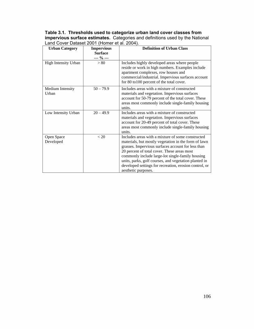
106
m impe l Land
UrbSurface --- % ---
Definition of Urban Class
Table 3.1. Thresholds used to categorize urban land cover classes frorvious surface estimates. Categories and definitions used by the Nationa Cover Dataset 2001 (Homer et al. 2004). an Category Impervious
High Intensity Urban > 80 Includes highly developed areas where peopreside or work in high numbers. Examples includeapartment complexes, row houses and commercial/industrial. Impervious surfaces account for
le
80 to100 percent of the total cover. Medium Intensity Urban
50 – 79.9 Includes areas with a mixture of constructed materials and vegetation. Impervious surfaces account for 50-79 percent of the total cover. These areas most commonly include single-family housing units.
Low Intensity Urban 20 – 49.9 Includes areas with a mixture of constructed materials and vegetation. Impervious surfaces account for 20-49 percent of total cover. These areas most commonly include single-family housing units.
Open Space Developed
< 20 Includes areas with a mixture of some constructed materials, but mostly vegetation in the form of lawn grasses. Impervious surfaces account for less than 20 percent of total cover. These areas most commonly include large-lot single-family housing units, parks, golf courses, and vegetation planted in developed settings for recreation, erosion control, or aesthetic purposes.
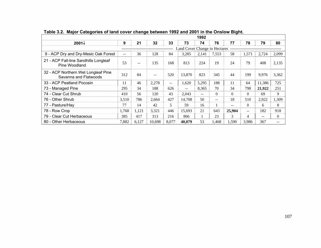
107
Table 3.2. Major Categories of land cover change between 1992 and 2001 in the Onslow Bight. 1992
2001↓ 9 21 32 33 73 74 76 77 78 79 80 ---------------- ------------------ La ver Chang Hectare ------------- ------------ nd Co e in s ------ ------ ----- 9 - ACP Dry and Dry-Mesic Oak Forest -- 36 128 84 2,14 55 1,571 24 3,285 1 7, 3 58 2,7 2,099
21 - ACP Fall-line Sandhills Longleaf Pine Woodland 53 -- 135 168 224 19 79 8 813 24 40 2,135
32 - ACP Northern Wet Longleaf Pine Savanna and Flatwoods 312 84 -- 520 13,870 82 34 9 76 3 5 44 19 9,9 3,362
33 - ACP Peatland Pocosin 11 46 2,278 -- 1,620 5,295 188 11 64 11,386 725 73 - Managed Pine 295 34 188 626 -- 8,365 70 34 798 21,922 251 74 - Clear Cut Shrub 410 56 120 43 2,043 0 0 -- 0 69 9 76 - Other Shrub 3,510 786 2,664 427 14 50 -- 510 ,708 18 2,922 1,309 77 - Pasture/Hay 77 14 42 5 59 1 -- 0 16 6 8 78 - Row Crop 1,768 1,121 3,321 446 15,693 21 643 25 -- 182,904 918 79 - Clear Cut Herbaceous 385 417 313 216 866 1 23 3 4 -- 0 80 - Other Herbaceous 7,882 6,127 1 7 0,698 8,077 40,079 53 1,468 1,590 3,986 36 --
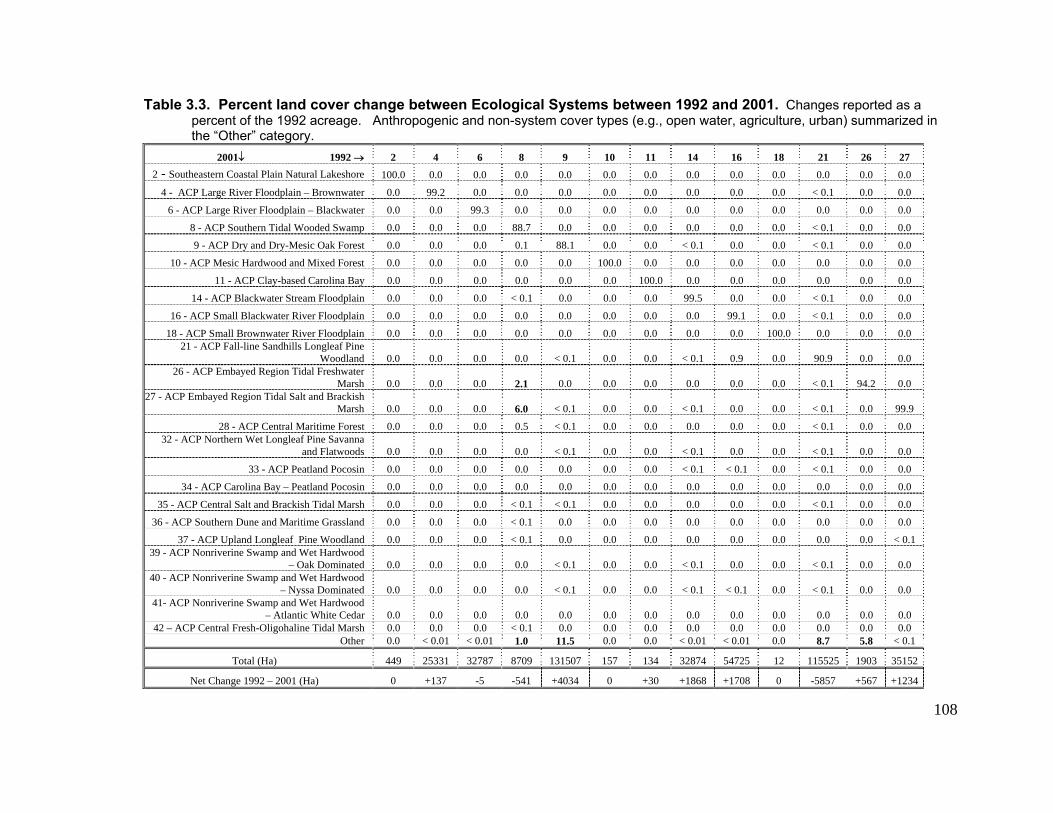
108
anges reported as a re, urban) summarized in
the “Other” ategory. 2001 1992 → 2
Table 3.3. Percent land cover change between Ecological Systems between 1992 and 2001. Chpercent of the 1992 acreage. Anthropogenic and non-system cover types (e.g., open water, agricultu
c↓ 4 6 8 9 10 11 14 16 18 21 26 27
2 - Southeastern Coastal Plain Natural Lakeshore 100.0 0. 0.0 0 0 0. 0.0 0.0 0 0. 0.0 0.0 .0 0 0.0 0.0 0.0
4 - ACP Large River Floodplain – Brownwater 0.0 99. 0. 0 0.0 0. 0.0 1 0 2 0 0. 0.0 0.0 0 0.0 < 0. 0. 0.0
6 - ACP Large River Floodplain – Blackwater 0. 0. 99.3 0 0. 0. 0 0.0 0 0 0. 0.0 0.0 0 0 0. 0.0 0.0 0.0
8 - ACP Southern Tidal Wooded Swamp 0.0 0.0 0.0 88.7 0.0 0.0 0.0 0.0 0.0 0.0 < 0.1 0.0 0.0
9 - ACP Dry and Dry-Mesic Oak Forest 0. 0.0 0.0 1 0. < 0. 0.0 0.0 1 0 0. 88.1 0.0 0 1 < 0. 0.0 0.0
10 - est 0.0 0.0 0.0 0.0 0.0 100.0 0.0 0.0 0.0 0.0 0.0 0.0 0.0 ACP Mesic Hardwood and Mixed For
11 - ACP Clay-based Carolina Bay 0.0 0.0 0.0 1 0. 0.0 0.0 0 0.0 0.0 0.0 00.0 0 0. 0.0 0.0
14 - ACP Blackwater Stream Floodplain 0. 0.0 0.0 .1 99. 0.0 0.0 1 0 < 0 0.0 0.0 0.0 5 < 0. 0.0 0.0
16 - ACP Small Blackwater River Floodplain 0. 0.0 0.0 0 0. 0. 99. 0.0 0.1 0.0 0. 0.0 0.0 0 0 1 < 0.0 0
18 - ACP Small Brownwater River Floodplain 0. 0.0 0. 0. 0 0.0 0.0 0 0.0 0.0 0.0 0 0 0. 10 0.0 0.0 0.0 21 - ACP Fall-line Sandhills Longleaf Pine
Woodland 0. 0.0 0.0 0. < 0. 0.9 .9 00 0.0 < 0.1 0.0 0 1 0.0 90 0.0 .0 26 - ACP Embayed Region Tidal Freshwater
Marsh 0. 0.0 0.0 1 0. 0. 0. 0.0 0.1 2 0.0 2. 0.0 0.0 0 0 0 < 94. 0 27 - ACP Embayed Region Tidal Salt and Brackish
Marsh 0. 0. 0. < 0. 0.0 0 99.0 0 0.0 6.0 < 0.1 0.0 0 1 0. < 0.1 0.0 9
28 - ACP Central Maritime Forest 0.0 0.0 0.0 0.5 < 0.1 0.0 0.0 0.0 0.0 0.0 < 0.1 0.0 0.0 32 - ACP Northern Wet Longleaf Pine Savanna
and Flatwoods 0.0 0.0 0.0 0.0 < 0.1 0.0 0.0 < 0.1 0.0 0.0 < 0.1 0.0 0.0
33 - ACP Peatland Pocosin 0.0 0.0 0.0 0.0 0.0 0.0 0.0 < 0.1 < 0.1 0.0 < 0.1 0.0 0.0
34 - ACP Carolina Bay – Peatland Pocosin 0.0 0.0 0.0 0.0 0.0 0.0 0.0 0.0 0.0 0.0 0.0 0.0 0.0
35 - ACP Central Salt and Brackish Tidal Marsh 0.0 0.0 0.0 < 0.1 < 0.1 0.0 0.0 0.0 0.0 0.0 < 0.1 0.0 0.0
36 - ACP Southern Dune and Maritime Grassland 0.0 0.0 0.0 < 0.1 0.0 0.0 0.0 0.0 0.0 0.0 0.0 0.0 0.0
37 - ACP Upland Longleaf Pine Woodland 0.0 0.0 0.0 < 0.1 0.0 0.0 0.0 0.0 0.0 0.0 0.0 0.0 < 0.1 39 - ACP Nonriverine Swamp and Wet Hardwood
– Oak Dominated 0.0 0.0 0.0 0.0 < 0.1 0.0 0.0 < 0.1 0.0 0.0 < 0.1 0.0 0.0 40 - ACP Nonriverine Swamp and Wet Hardwood
– Nyssa Dominated 0.0 0.0 0.0 0.0 < 0.1 0.0 0.0 < 0.1 < 0.1 0.0 < 0.1 0.0 0.0 41- ACP Nonriverine Swamp and Wet Hardwood
– Atlantic White Cedar 0.0 0.0 0.0 0.0 0.0 0.0 0.0 0.0 0.0 0.0 0.0 0.0 0.0 42 – ACP Central Fresh-Oligohaline Tidal Marsh 0.0 0.0 0.0 < 0.1 0.0 0.0 0.0 0.0 0.0 0.0 0.0 0.0 0.0
Other 0.0 < 0.01 < 0.01 1.0 11.5 0.0 0.0 < 0.01 < 0.01 0.0 8.7 5.8 < 0.1
Total (Ha) 449 25331 32787 8709 131507 157 134 32874 54725 12 115525 1903 35152
Net Change 1992 – 2001 (Ha) 0 +137 -5 -541 +4034 0 +30 +1868 +1708 0 -5857 +567 +1234
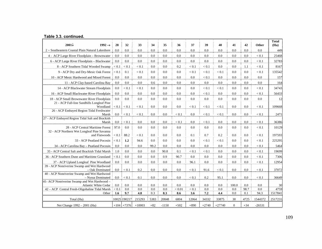
109
1992 → 28 32 33 34 35 36 37 39 40 41 42 Other (Ha)
Table 3.3. continued.
2001↓ Total
2 - Southeaster 0.0 0. 0. 0. 0. 0. 0. 0. 9n Coastal Plain Natural Lakeshore 0 0 0 0 0.0 0.0 0 0.0 0.0 0 0 44
4 - ACP Large River Floodplain – Brownwater 0.0 0. 0. 0. 0. 0. 0. < 0. 80 0 0 0 0.0 0.0 0 0.0 0.0 0 1 2546
6 - ACP Large River Floodplain – Blackwater 0. 0.0 0. 0. 0. 0. 0. < 0. 30 0 0 0 0.0 0.0 0 0.0 0.0 0 1 3278
8 - ACP Southern Tidal Wooded Swamp < 0. < 0.1 < 0. 0.0 0.0 0.2 < 0.1 < 0. 0.0 0. 1.1 < 0.1 1 1 0 1 8167
9 - ACP Dry and Dry-Mesic Oak Forest < 0.1 < 0.1 0.0 0 0.0 < 0.1 < 0. < 0. 0. 0. < 0. 1 20.1 0. 1 1 0 0 1 3554
10 - A 0. 0.0 0.0 0.0 0.0 0.0 0.0 < 0. 0.0 0. 0. 0.0 7CP Mesic Hardwood and Mixed Forest 0 1 0 0 15
11 - ACP Clay-based Carolina Bay 0. 0.0 0.0 0.6 0.0 0.0 0 0.0 0.0 0. 0.0 0.0 40 0. 0 16
14 - 0. < 0.1 < 0.1 0.0 0.0 0.0 0.0 < 0. < 0. 0. 0.0 < 0. 3 ACP Blackwater Stream Floodplain 0 1 1 0 1 3474
16 - 0. 0.0 0. 0.0 . < 0. 0. 0. < 0. 3ACP Small Blackwater River Floodplain 0 0 0 0 0.0 0.0 1 0 0.0 0 1 5643
1 0. 0. 0. 0. 0. 0. 0. 0. 28 - ACP Small Brownwater River Floodplain 0 0 0 0 0 0.0 0.0 0 0.0 0.0 0 0 121 - ACP Fall-line Sandhills Longleaf Pine
Woodland < 0. < 0.1 < 0.1 0.0 0.0 0.0 < 0.1 < 0.1 < 0. 0. 0.0 < 0. 681 1 0 1 109626 -
0. < 0.1 < 0.1 0.0 0.0 < 0.1 0.0 < 0. < 0. 0.0 0.0 < 0. ACP Embayed Region Tidal Freshwater
Marsh 0 1 1 1 247127 - ACP
0. < 0.1 0.0 0.0 0.0 < 0.1 0.0 < 0.1 0.0 0.0 0.0 < 0. 6Embayed Region Tidal Salt and Brackish
Marsh 0 1 3638
28 - ACP Central Maritime 97. 0. 0. 0. 0. 0. 0. < 0.Forest 0 0 0 0 0 0.0 0.0 0 0.0 0.0 0 1 1012932 - ACP Nor
0. 88. < 0. 0. 0. 0. 0. < 0. 93thern Wet Longleaf Pine Savanna
and Flatwoods < 1 2 1 0 0 0.0 0.1 7 0.2 0.0 0 1 1975
33 - ACP Pe < 0. 1.2 94.6 0.0 0.0 0 0.0 < 0. < 0. 0. 0. < 0. 2 5atland Pocosin 1 0. 1 1 0 0 1 2529
34 - ACP Caro 0. 0.0 0.0 99.2 0.0 0.0 0.0 0. 0. 0. 0. < 0.lina Bay – Peatland Pocosin 0 0 0 0 0 1 5464
35 - A 1. 0.0 0.0 0.0 90.8 0.1 < 0.1 < 0. 0.0 0. 0.0 < 0. 9CP Central Salt and Brackish Tidal Marsh 0 1 0 1 1969
3 < 0. 0.0 0 . 0. 0. 0. 0. 0. < 0. 66 - ACP Southern Dune and Maritime Grassland 1 0.0 0. 0 9 90.7 0 0 0 0 0 1 730
37 - ACP Upland Longleaf Pine Woodland 0. 0.0 0.0 0.0 .0 0.0 96.1 0.0 0.0 0. 0.0 < 0. 40 0 0 1 129539 - A
0. < 0.1 0.2 0.0 0.0 0.0 < 0.1 91.6 < 0. 0.0 0.0 < 0. 2CP Nonriverine Swamp and Wet Hardwood
– Oak Dominated 0 1 1 370740 - ACP Nonriverine Swamp and Wet Hardwood
– Nyssa Dominated 0. < 0.1 0.1 0.0 0.0 0.0 < 0.1 0.2 95.1 0.0 0.0 < 0. 90 1 366441-
0. 0. 0. 0. 0. 0. 100.0 0. 0. 30 ACP Nonriverine Swamp and Wet Hardwood –
Atlantic White Cedar 0 0 0 0 0 0.0 0.0 0 0.0 0 0 42 – ACP Central Fresh-Oligohaline Tidal Marsh < 0.0 0.0 0.0 0.0 0.01 < 0.1 0.0 0.0 0. 98. 0.0 90.1 < 0 7 475
Other 1. 9.7 4.8 0.3 . 7. 0. 94. 15 16 8 3 8.6 3.6 2 4.4 0 0.1 3 1784
Total (Ha) 1002 1902 5383 20848 6804 1206 3433 3387 30 4725 15445 17 215293 4 2 5 372 2517231
Net Change 1992 Ha) +7376 +10003 +502 +890 – 2001 ( +104 +82 -1150 +2740 +27740 0 +34 -26531
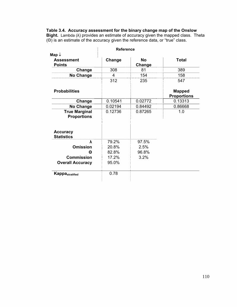
110
Table 3.4. Accuracy assessment for the binary change map of the Onslow Bight. Lambda (λ) provides an estimate of accuracy given the mapped class. Theta
c h , “
Reference
(Θ) is an estimate of the ac uracy given t e reference data or true” class.
Map ↓ Assessment Points
aChange
Ch nge No Total
Change 03 8 81 389 No Change 4 154 158
312 235 547
Probabilities Mapped rP oportions
Change 0.02772 0.13310.10541 3 No Change 0.02194 0.86660.84492 8
True Marginal Proportions
20.1 736 0.87265 1.0
Accuracy Statistics
λ 79.2% 97.5% Omission .20 8% 2.5%
Θ 82.8% 96.8% Commission 17.2% 3.2%
Overall Accuracy
.
95 0%
Kappastratified .0 78
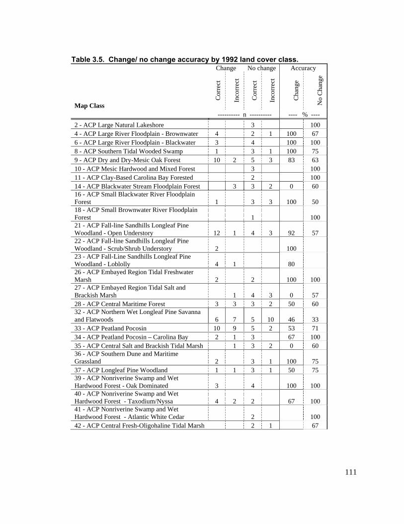
111
Ta
ble 3.5. Change/ no change accuracy by 1992 land cover class. Change No change Accuracy
Map
Inco Cor
rect
Inco
rrec
t
Cha
nge
Cha
nge
Class
Cor
rect
rrec
t
No
------ ---- ---- ---- -----n - % ----2 - ACP Large N e atural Lakeshor 3 100 4 - ACP Large R ownw 4 1 100 iver Floodplain - Br ater 2 676 - ACP Large River Floodplain - ackw 3 100 Bl ater 4 100 8 - AC Wooded S amp 1 1 10P Southern Tidal w 3 0 75 9 - AC esic Oak F rest 1 2 3 P Dry and Dry-M o 0 5 83 63 10 - ACP Mesic Har ed dwood and Mix Forest 3 100 11 - ACP Clay-B a Fo ased Carolina B y rested 2 100 14 - ACP Bl lai 2 0 ackwater Stream Floodp n Forest 3 3 60 16 - ACP Sm r loodForest 1 3 3 100
all Blackwater Rive F plain 50
18 - ACP Small Br wnwater Rive loodpla Forest 1 0
o r F in10
21 - A andhills Long af Pine Wood nderstory 12 1 4 3 92 57
CP Fall-line Sland - Open U
le
22 - ACP Fall-line Sandhills Long af PiWoodland - Scrub to 2 100
le ne /Shrub Unders ry
23 - ACP Fall-Lin g af PWoodland - L 4 80
e Sandhills Lon le ine oblolly 1
26 - ACP l FreshwMarsh 2 2 100 0
Embayed Region Tida ater 10
27 - ACP Embayed Region Tidal Salt and Bracki 1 4 3 0 sh Marsh 57 28 - ACP Central Maritime Forest 3 3 3 2 50 60 32 - ACP Northern Wet Longleaf Pine Savanna and Flatwoods 6 7 5 10 46 33 33 - ACP Peatland Pocosin 10 9 5 2 53 71 34 - ACP Peatland Pocosin – Carolina Bay 2 1 3 67 100 35 - ACP Central Salt and Brackish Tidal Marsh 1 3 2 0 60 36 - ACP Southern Dune and Maritime Grassland 2 3 1 100 75 37 - ACP Longleaf Pine Woodland 1 1 3 1 50 75 39 - ACP Nonriverine Swamp and Wet Hardwood Forest - Oak Dominated 3 4 100 100 40 - ACP Nonriverine Swamp and Wet Hardwood Forest - Taxodium/Nyssa 4 2 2 67 100 41 - ACP Nonriverine Swamp and Wet Hardwood Forest - Atlantic White Cedar 2 100 42 - ACP Central Fresh-Oligohaline Tidal Marsh 2 1 67
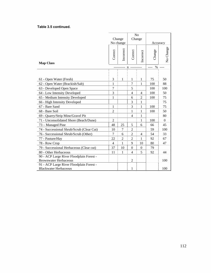
112
able 3.5 continued.
Change ha
Change racy
T
No c nge
No
Accu
Cor
rect
o
Cor
rect
ang
Inc
Inco
rrec
t
rrec
t
Ch
No
e
Cha
nge
Map Class ------- n ----- -- ----- ---- - - %- -- 61 - Open Water (Fresh) 3 1 1 1 75 50 62 - Open Water (Brackish/Salt) 1 7 1 100 88 63 - Developed Open Space 7 5 100 100 64 - Low Intensity Developed 3 4 4 1 00 50 65 - Medium Intensity Developed 1 6 2 1 00 75 66 - High Intensity Developed 3 1 75 67 - Bare Sand 1 3 1 100 75 68 - Bare Soil 2 1 1 1 00 50 69 - Quarry/Strip Mine/Gravel Pit 4 1 80 71 - Unconsolidated Shore (Beach/Dune) 2 1 100 0 73 – Managed Pine 48 25 5 6 66 45 74 - Successional Shrub/Scrub (Clear Cut) 1 10 7 2 59 0076 - Successional Shrub/Scrub (Other) 7 6 2 4 54 33 77 - Pasture/Hay 22 2 2 1 92 67 78 - Row Crop 4 1 9 10 80 47 79 - Successional Herbaceous (Clear cut) 37 10 0 0 79 80 - Other Herbaceous 11 1 4 5 92 44 90 - ACP Large River Floodplain Forest - Brownwater Herbaceous 2 100 91 - ACP Large River Floodplain Forest - Blackwater Herbaceous 1 100
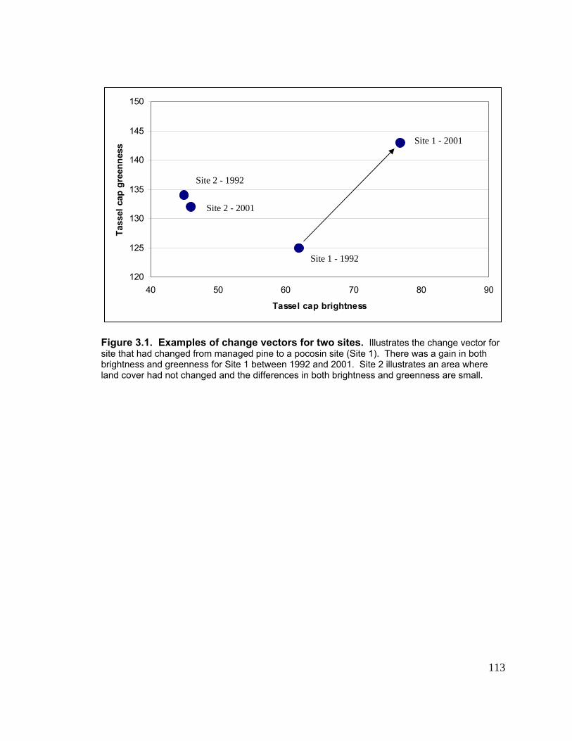
113
ange vector for s to a p in s a gain in both b etween 1992 and 01. ite lust re l t changed and the differences th brightness gr ss are small.
Figure 3.1. Examples of change vectors for two sites. Illustrates the chite that had changed from managed pine ocos site (Site 1). There warightness and greenness for Site 1 b 20 S 2 il rates an area whe
and cover had no in bo and eenne
120
125
130
l
135
140
145
150
50 60 7 90
Tassel p br htn
cap
gr
ness
40 0 80
ca ig ess
Tass
eee
n
Site 1 - 1992
Site 1 - 2001
Site 2 - 1992
Site 2 - 2001
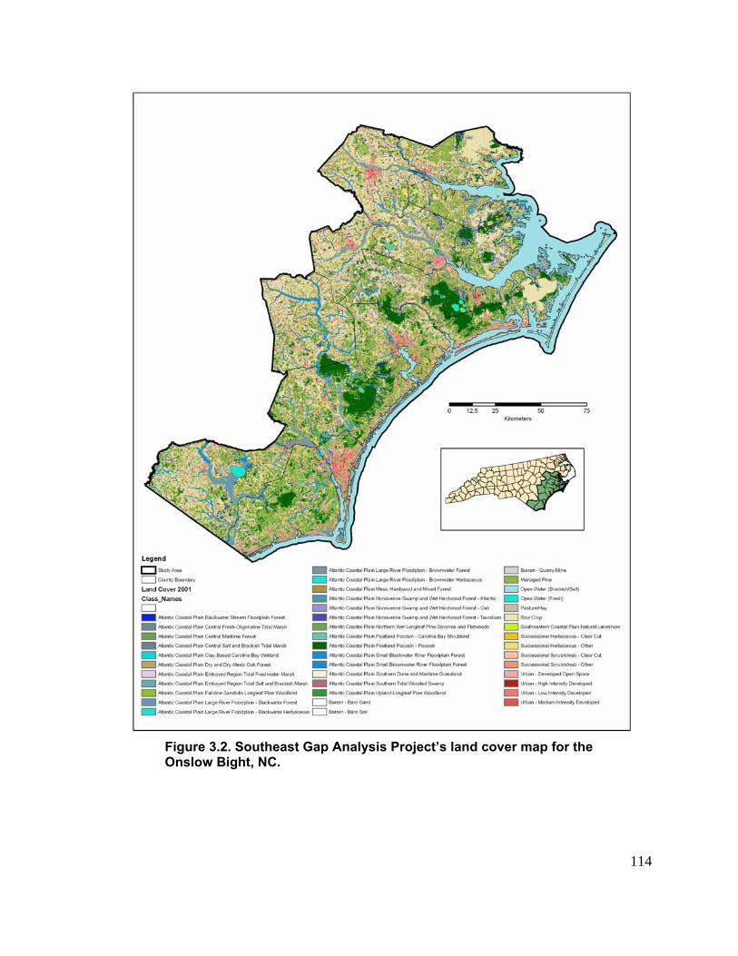
Figure 3.2. Southeast Gap Analysis Project’s land cover map for the Onslow Bight, NC.
114
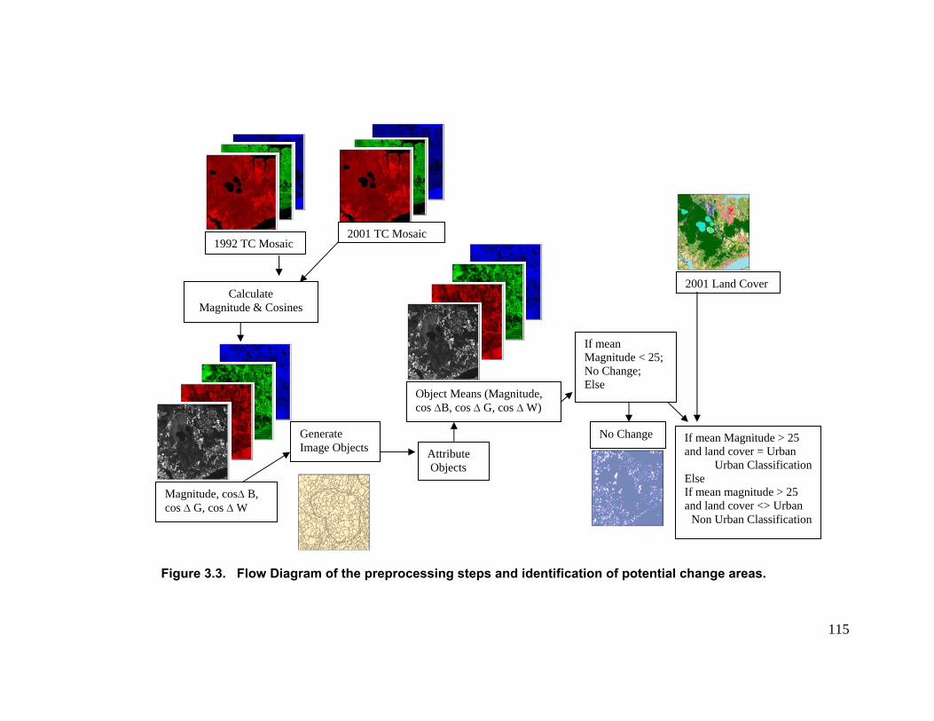
115
w Diagram of the preprocessing steps and identification of potential change areas.
2001 TC Mosaic1992 TC Mosaic
Figure 3.3. Flo
Calculate gnitude & Cosines Ma
Magni , cosD B, cos D os D W
tudeG, c
Generate Image Objects
2001 Land Cove
Object Means (Magnitude, cos DB, cos D G, cos D W)
If mean Magnitude < 25; No Change; Else
r
No Change If mean Magnitude > 25 and land cover = Urban
Urban ClassificationElse If mean magnitude > 25 and land cover <> Urban
Non Urban Classification
Attribute Objects
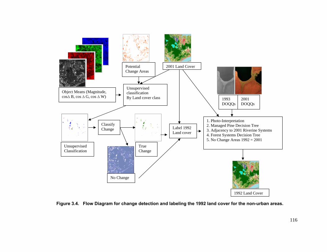
116
areas.
Potential Change Areas
2001 Land Cover
Figure 3.4. Flow Diagram for change detection and labeling the 1992 land cover for the non-urban
Unsupervised classification By Land cover class
Unsupervised Classification
Object Means (Magnitude, cosD B, cos D G, cos D W) 1993
DOQQs 2001 DOQQs
1. Photo-Interpretation 2. Managed Pine Decision Tree 3. Adjacency to 2001 Riverine Systems 4. Forest Systems Decision Tree 5. No Change Areas 1992 = 2001
ClassifyChange Label 1992
Land cover
True Change
No Change
1992 Land Cover
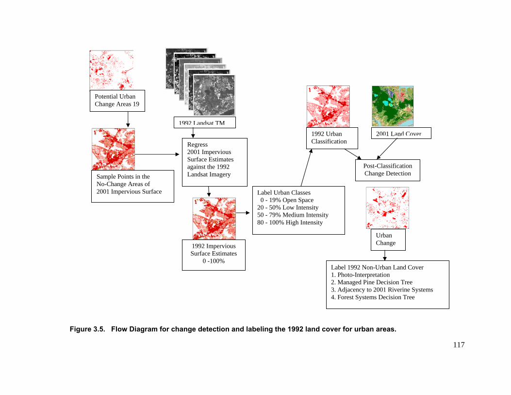
117
Figure 3.5. Flow Diagram for change detection and labeling the 1992 land cover for urban areas.
Potential Urban Change Areas 19
1992 Landsat TM
1992 Urban Classification
2001 Lan
Sample Points in the No-Change Areas of 2001 Impervious Surface
Regress 2001 Impervious Surface Estimates against the 1992 Landsat Imagery
1992 Impervious Surface Estimates
0 -100%
d Cover
Post-Classification Change Detection
Label Urban Classes 0 - 19% Open Space 20 - 50% Low Intensity 50 - 79% Medium Intensity 80 - 100% High Intensity
Urban Change
Label 1992 Non-Urban Land Cover 1. Photo-Interpretation 2. Managed Pine Decision Tree 3. Adjacency to 2001 Riverine Systems 4. Forest Systems Decision Tree
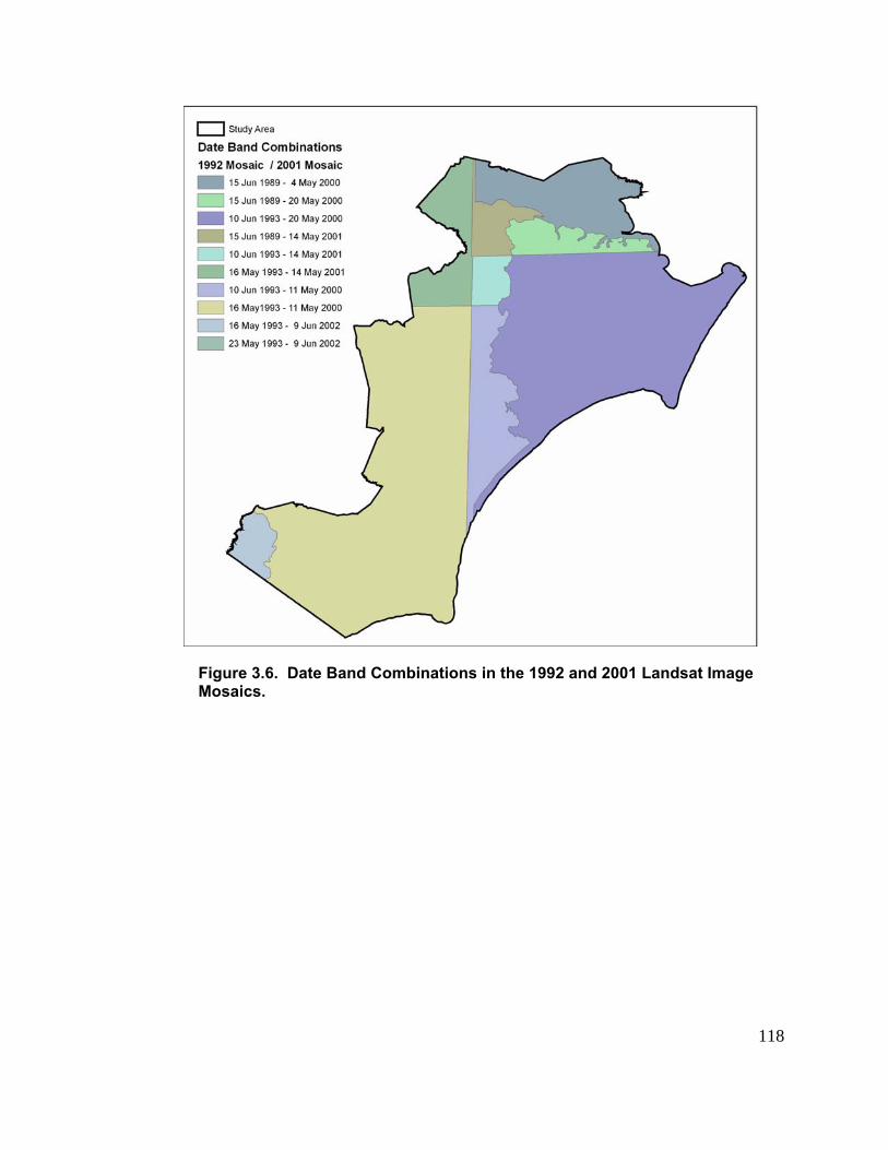
118
Figure 3.6. Date Band Combinations in the 1992 and 2001 Landsat Image Mosaics.
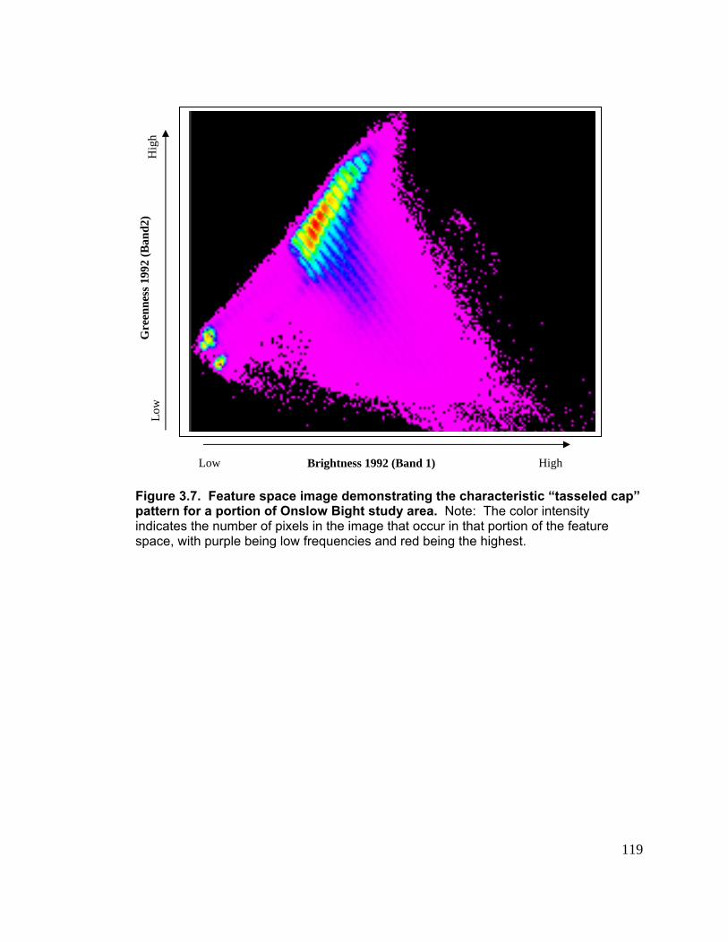
119
Figure 3.7. Feature space image demonstrating the characteristic “tasseled cap” pattern for a portion of Onslow Bight study area. Note: The color intensity indicates the number of pixels in the image that occur in that portion of the feature space, with purple being low frequencies and red being the highest.
Brightness 1992 (Band 1) Low High
Gre
enne
ss 1
992
(Ban
d2)
Low
H
igh
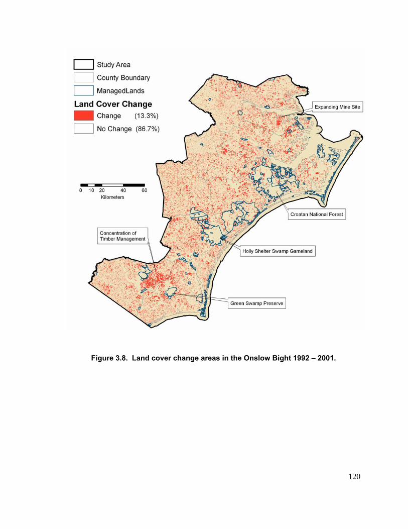
120
Figure 3.8. Land cover change areas in the Onslow Bight 1992 – 2001.
121
Tools for assessing and monitoring conservation status: A case study from the Onslow Bight, NC. Alexa J. McKerrow, Thomas R. Wentworth, Jaime A. Collazo, Martha J. Groom, George R. Hess, and Heather M. Cheshire. Abstract The National Gap Analysis Program (GAP) has as its mission “keeping common species
common”. In support of that mission the program has conducted and funded research
during the past decade with the goal of providing three key datasets used to assess
conservation status: detailed land cover, predicted distributions of terrestrial vertebrate
species based on application of habitat models, and land stewardship. We explored the
use of these datasets in combination with a change detection analysis to assess the
conservation status of Ecological Systems and vertebrate species of the Onslow Bight
Landscape. We modeled predicted distributions for 141 priority vertebrate species
identified in the North Carolina State Wildlife Action Plan (SWAP) and by Partners in
Flight (PIF) as the basis for our conservation assessment. We were specifically
interested in three general questions:
• Were there gains or losses in the extent of Ecological Systems and species
predicted distributions between 1992 and 2001?
• When translated to a spatial framework, was there agreement on the ground
between agency priorities?
• How well did the conservation network do with respect to capturing priority areas?
By integrating species models from the two dates, we were able to quantify the gains
nd losses of the priority species for the two programs. Using the 2001 version of the
redicted distribution models, we mapped richness hotspots for the two agency lists.
The h nd
areas with at least 13 of the PIF priority species, included nearly one-third (32%) of the
landscape. Forty-seven percent of the area did not meet the hotspot criteria for either
list and twenty-one percent met the criteria for one agency or the other. When we
compared the hotspot maps to the existing conservation lands and new acquisitions, we
found that both existing conservation lands and the newly acquired easements were
biased toward the hotspots, with 70% of the existing conservation network on lands that
met the hotspot criteria for both agencies, and 50% of the new acquisitions doing the
a
p
otspots for the two lists, areas with at least 28 of the SWAP priority species a
122
ent of the change in status of species habitat over time.
e Wildlife Action Plans, artners in Flight, Bird Conservation Region, Complementarity Analysis
d
ed
y
species (e.g., food, fiber, and medicine) and the
tact
ity (Callicott 2006, Edwards-Jones
sthetic
ation of biological diversity.
l.
same. The approach outlined is responsive to individual agency priorities and allows for
n objective assessma
Keywords: Ecological Systems, Gap Analysis Program, StatP Introduction The Case for Spatially Explicit Conservation Tools
More than four decades ago the decline in biological diversity was officially recognize
as an international crisis. In the early 1960s the World Conservation Union started the
IUCN Red List to identify endangered species. Today that list includes 41,415 species,
and 16,360 of them are considered threatened (IUCN 2007). The United States follow
suit in 1966 with the Endangered Species Preservation Act (1966) and the subsequent
Endangered Species Act (1973). In both cases, the need for maintaining diversity b
conserving individual species was seen as central to the welfare of people.
The list of material benefits provided by
potential for future innovations and discoveries (option values) provided for by in
natural systems motivate the conservation of biodivers
2006; Scott et al. 1995). Finally, individuals and communities have ethical and ae
values directly tied to the conserv
Even with the incentives to conserve biodiversity, the number of listed species is
increasing and deleterious changes in the landscape are out-pacing our knowledge.
Once listed, the cost to maintain a species can be high and long-lasting. As Scott et a
(2005) summarized, recovery is best described as a continuum; once endangered, a
species may be “conservation – reliant”, requiring constant intervention. Unfortunately,
for many species an accurate understanding of their status is impossible to assess.
Wilcove and Master (2005) suggest that the data for 85% of the species (plants,
animals, and fungi) in the United States are insufficient to determine their status
accurately. Without a complete inventory, conservationists rely on surrogates for
biodiversity (e.g., indicator species, keystone species, and species guilds) to identify
conservation priorities.

123
ster
005) suggest one alternative favored by many conservation biologists - the use of a
n.
nty years, the National Gap Analysis Program has been advocating a
Scott et al. saw the power of
is
two
dicators of biodiversity (Scott et al. 1993, Scott and Jennings 1998). Since the
ate the gap data into their
gency-specific analyses. Two of the most promising collaborations include State
Given the level of the threats, the rate of change, and the lack of a complete
assessment, we need proactive approaches to conservation. Wilcove and Ma
(2
“coarse-filter” approach to protection, with ecological communities acting as the scree
For nearly twe
coarse filter approach to planning. As early as 1993
analyzing biodiversity data in a spatial context. In the preface to the 2000 issue of the
special edition of Landscape Ecology devoted to the use of gap analysis, Burke (2000)
suggested that the intersection of landscape ecology and conservation biology was the
most promising front for effective species conservation.
Assuming the cost of conservation is lower for intact systems, the National Gap Analys
Program has been developing land cover and vertebrate species richness as
in
program was initiated many changes have occurred in the technology and the methods
have evolved, but the concept remains the same: proactively manage biological
diversity to keep common species common.
Most recently, the GAP has actively engaged partners to integr
a
Wildlife Action Plans (SWAPs) and the Partners in Flight (PIF).
Ongoing Conservation Planning Efforts
State Wildlife Action Plans Recently State and Tribal Wildlife Agencies in the U.S. developed their first
comprehensive State Wildlife Action Plans (SWAPs). Those plans were required bef
those agencies would be eligible for funding through the Wildlife Conservation an
Restoration Program. For many state agencies this was the first time they had ac
funding specifically for the management of non-game and non-threatened and
endangered species. In order to fulfill the guidelines set out by Congress, each plan h
to address eight require
ore
d
cess to
ad
d elements (Table 4.1, USFWS 2007). Once an agency
ompleted its plan, it had access to funding to implement the work outlined in the plan. c
124
abitat patches in the identification of priorities, sharing maps of priority habitats and
ecies
In a review of the action plans specific to urbanization, Defenders of Wildlife (2006)
identified some key components that would make planning most effective. Some of
those included protecting priority species and habitats, protecting connectivity and large
h
priority conservation areas, and giving planners spatial data that identify sensitive
resources. Each of these components depends on spatially explicit data tied to sp
habitats and land management.
Partners in Flight Partners in Flight (PIF) is a consortium of government and non-government agencies
nd individuals working to conserve bird species. The partnership formed in 1990 in
ed
ecies in
ss, assessing the status and trends for
ach avian species, and then setting priorities on the continental and regional scales
ervation Regions – BCR)
cale based on a weighted scoring process to identify species of continental concern. A
p species, identifies as species with a large
within a single avifaunal biome for a part of the life cycle
e regional
e to
Study Objectives
a
response to the declining populations of migratory land birds. In order to address the full
range of issues related to these species, the consortium works both within the Unit
States and internationally to develop conservation plans and to identify priority sp
need.
The PIF planning process is a two stage proce
e
(Panjabi et al. 2005). Each species is assessed based on size criteria related to
population trends, species distribution, and threats (Table 4.2, Rich et al. 2004).
Priorities are then set at the continental and regional (Bird Cons
s
second category, continental stewardshi
percentage of their population
(breeding season, non-migratory portion of the non-breeding season). At th
scale priorities are set based on scoring criteria that link regional and continental scores.
Species of regional concern are those that have high regional scores, are vulnerabl
threats within the region, and where the representation within a region is proportionally
high relative to the global distribution.
125
arly in its history, the Gap Analysis Program identified areas of high species richness
993,
f
ur objective in this study was to create a database that provides a spatial framework
eporting with respect to the overall GAP goal of keeping common
fic
s in Flight.
nd
ies
s of
rs.
,
ardwood forests and cypress gum swamps.
oncentrations of pond pine woodlands and nonriverine swamps and wet hardwoods
ccur within what Omernik classifies as the Swamps and Peatlands ecoregion. The
arolinian Barrier Islands and Coastal Marshes support narrow strands of maritime
E
outside the existing conservation network as priorities for conservation (Scott et al. 1
Kiester et al. 1996). A “gap” represented an area in the landscape that was not being
managed for biodiversity but did represented habitat for a high number of terrestrial
vertebrates. Over time the GAP datasets have evolved to better address the needs o
natural resource agencies, each of which have their own prioritization schemes or
mandates.
O
for monitoring and r
species common, while at the same time tailoring the analyses to our partners. We
wanted to design an approach based on Gap Analysis Program datasets that could be
applied to a variety of conservation questions. Specifically, we wanted to test the
applicability of the GAP datasets and a change analysis in addressing questions speci
to the priority species lists for the North Carolina Wildlife Resources Commission and
Partner
Study Area The Onslow Bight study area includes parts of 13 counties in Coastal North Carolina a
covers an area of 250,000 km2. Eight of Omernik’s Level IV ecoregional boundar
intersect the study area (Figure 4.1; EPA 2004). Having been settled for hundred
years, the area has undergone tremendous change. Much of the landscape today is
dominated by agriculture and timber production (Auch 2006), with concentrations of
urban growth centered in Wilmington, New Bern, and along the transportation corrido
The Onslow Bight supports a diversity of plant communities, some of which have had
their extents reduced dramatically by the history of settlement in the area. Historically
the Carolina Flatwoods region supported a matrix of longleaf pine woodland (Frost 2006
Frost 1993). The Mid-Atlantic Floodplains and Low Terraces (EPA 2004) bisect the area
and are characterized by bottomland h
C
o
C
126
was mapped using 2001 satellite imagery for the Onslow Bight as a part of
e Southeastern Gap Analysis Project. The resulting land cover map was developed
on
ed on a stratified sampling was 0.75. Per-class accuracies for the
cological Systems varied considerably. For a complete description of the methods and
AP land cover, had been developed using different methods and map legend
forest and dune vegetation in the uplands and vast expanses of salt and brackish
marshes occur on the landward side of the barrier islands and in protected portions of
the embayed region to the north.
Methods
Land Cover Mapping
Land cover
th
using Landsat TM satellite imagery as the baseline dataset. In that map, the general
land cover classes (for example, water, agriculture, and urban) were incorporated from
the National Land Cover Dataset (NLCD 2001), while the vegetated classes were
mapped using a combination of expert derived decision rules, image objects, and
decision tree models (Chapter 2 this volume). The Ecological Systems Classificati
(Comer et al. 2003) was the basis for the map legend. A total of forty two land cover
classes were included in the final map legend. Overall accuracy was 77% and the
Kappa statistic bas
E
results for the land cover map, refer to Chapter 2.
Change Detection
In order to quantify the changes in the extent of land cover and predicted distributions for
species, we used two versions of the land cover map, one representing the 1992 time
period and another for 2001. As mentioned above, a 2001 Ecological Systems map had
been created already. The only 1992 land cover for the study area, the North Carolina
G
(McKerrow et al. 2006). To create a map for 1992 that was consistent with the 2001
map, we used a spectral change detection process to identify areas of potential change,
we then labeled the 1992 map for areas that had changed and labeled unchanged areas
with the 2001 land cover classes. The two land cover maps were used to characterize
the changes in Ecological Systems and predicted species distributions in the
assessment phase of this work.
127
entify
ges from 1992 and 2001. Areas with a high
agnitude of change between the two dates were identified as potential change areas.
s were then classified with respect to the 1992 land cover class. For the non-
s potentially changed, an unsupervised classification was used
t
ision
he
al.
om sample. For a complete
escription of the change detection, see Chapter 3.
a to map
4.3). Appendix 4.1 includes the list of the specific
abitat modeling parameters used for the species in this study.
To create the 1992 land cover map, a change vector analysis (CVA) was used to id
areas of potential change between 1992 and 2001. The change vectors were calculated
from tasseled cap transformed ima
m
Those area
urban areas identified a
to identify “true change” areas. That classification was based on the difference image
(magnitude) of change and the direction of change between 1992 and the 2001 Landsa
imagery.
Areas of change in non-urban areas were then labeled with respect to the types of
change that had occurred by one of three methods, aerial photo-interpretation, dec
rules based on ancillary data, or decision tree modeling. Urban areas identified as
potential change areas were mapped using impervious surface estimation, similar to t
approach used in the 2001 NLCD land cover dataset (Homer et al. 2004, Homer et
2007, and Yang et al. 2003). We estimated a net change of 13% for the study area
between 1992 and 2001. The accuracy of the change/no change map was estimated at
95% with a Kappa of 0.78 based on a stratified rand
d
Species Modeling
The Southeast Gap Analysis Program has developed a database for 614 terrestrial
vertebrate species that occur in the nine southeastern states (AL, FL, GA, KY, MS, NC,
SC, TN, and VA). The database includes information on key parameters needed to
model predicted distributions of habitat for each of those species. The database
represents a compilation of literature and expert opinion. Reviews of the habitat
parameters were conducted by project personnel at each of the three universities
involved in the Southeast Gap Analysis Project (North Carolina State University,
University of Georgia, and Auburn University). The models integrate species range
maps, habitat affinity information (suitable land cover types), and ancillary dat
the predicted distributions (Table
h
128
, 153
over. For model parameters derived directly from the land cover (e.g., patch
ize, edge, or urban avoidance) we created two versions of each data layer (1992 and
land
rom
ments
ap Analysis Program’s
tewardship provided information about the management status (a critical attribute) in
ion about who owns and manages the land (Crist 2000). There are
ach
ed
nnel
to
y
ts the conservation
asements that have been put in place by the state. Those easements can be acquired
Based on the North Carolina GAP data, more than 300 terrestrial vertebrate species had
a portion of their range within the study area (McKerrow et al. 2006). As a part of the
later regional effort, the Southeast GAP modeled distributions for 47 amphibians
birds, 53 mammals, and 63 reptiles that had with some portion of their distribution
predicted to occur in the Onslow Bight.
In this study, we used Southeast GAP’s vertebrate database to create two models for
each species of interest, one based on the 1992 land cover and another based on the
2001 land c
s
2001) for use in the habitat modeling. For ancillary data layers not derived from the
cover (e.g., species range maps, landforms), we assumed no change had occurred in
the 9 year period. The only model parameters that did change were those derived f
the 1992 and the 2001 land cover maps.
Land Stewardship Data
We used the Southeast Regional GAP Stewardship dataset for land ownership and
management information. That dataset covers nine southeastern states and docu
state and federal ownership and management. The G
S
addition to informat
four Status categories as defined by GAP (Table 4.4). A gap status is assigned for e
parcel based on a series of decisions that characterize the permanence of protection,
management intent, and the scope and extent of management activities (Figure 4.2).
The assignment of the gap status was based on information gathered from publish
descriptions of agency mandates, management plans, or interview with key perso
responsible for management of a parcel.
We wanted to study the new land acquisitions with respect to their placement relative
priority areas identified by the analysis. The most comprehensive dataset that tracks
acquisition dates consistently is the conservation easements database maintained b
the North Carolina State Properties Office. That dataset represen
e

129
a.
nalysis
r
d
hile those under-represented types became a primary focus for our land cover
of natural vegetation in the region makes it difficult to justify
n
s within the study area with less than 10% of
e distribution within Status 1 and 2 lands.
through agreements with the full range of land owners (e.g., private, non-governmental
organization, local government), but the easement is held by the state of North Carolin
Therefore we restricted our analysis of the new acquisitions to only the properties with
conservation easements acquired by the state since 1992.
AGap Analysis
In a separate effort, a preliminary gap analysis of the Southeastern Regional land cove
types was conducted by intersecting the regional Stewardship database with the nine
state land cover map (Table 4.5). We used a threshold of 10% of the mapped
distribution to identify gap cover types. From that analysis, eight of the Ecological
Systems in the Onslow Bight were identified as gaps with less than 10% of their mappe
distributions on GAP Status 1 and 2 lands throughout the region.
W
analysis, the historic loss
ignoring even those types that are considered well-represented in the conservation
network. Therefore, we included Ecological Systems that are currently well-represented
in our discussions.
We performed a gap analysis for the Onslow Bight for the Ecological Systems and
terrestrial vertebrates identified as priorities in the NC SWAP and PIF plans. We
intersected the mapped distribution of the element (Ecological System or vertebrate
species) within the Onslow Bight with the stewardship data and calculated the proportio
of each ecological system and vertebrate species’ predicted distribution represented in
Status 1, 2, 3 or 4 lands (water bodies greater than 40 ha were excluded). Gaps were
then identified as any land cover or specie
th
State Wildlife Action Plan
The North Carolina Wildlife Resources Commission went through an elaborate process
of interviewing biologists and conducting public forums to identify the species of greatest
130
winter residents as well as
nes that rarely breed in the state (Table 4.6). Our analysis included 123 terrestrial
species that occur in the Onslow Bight (20 amphibians, 56 birds, 15
32 reptiles). The complete list of the priority species and the criteria used
ners
ad also been
entified as priorities in the SWAP; so 18 PIF continental or regional priority species are
and vertebrate species. We decided to use a scorecard process, in
hich gains and losses are categorized into one of five categories - major losses, minor
t of
nd
by
++ a gain of over 20%
conservation concern for the first State Wildlife Action Plan (NCWRC 2005). That plan
identified 214 terrestrial vertebrates as priorities, including 29 subspecies. The
Southeast GAP had modeled 205 of these species in North Carolina. The nine species
in the SWAP that were not modeled by GAP included several
o
vertebrate
mammals, and
to select them in the SWAP are included in Appendix 4.2.
Partners in Flight
Thirty-eight avian species that occur in the Onslow Bight have been ranked by Part
in Flight as of regional or continental concern for the Southeastern Coastal Plain Bird
Conservation Region (BCR 27; Table 4.7). Twenty of those taxa h
id
unique to this list.
Scorecard Process
We needed an efficient method for summarizing the gains and losses of areas of the
Ecological Systems
w
loss, no change, minor gain, major gains - that could be summed by taxa or for a lis
Ecological Systems or priority species. Scorecards for both Ecological Systems a
priority species were developed by summarizing the 1992 and 2001 mapped extents
management status. Based on the changes in predicted distributions between 1992 and
2001 each element was assigned one of the following five categories:
- - a loss of greater than 20% in the predicted distribution occurred - a loss of between 5 and 20% 0 no difference - 5 to + 5% + a gain of between 5 and 20%
131
magery.
nd
nd a
he gains and losses in acreage for each element were calculated by summarizing the
d (Ecological System) or predicted distribution (vertebrate species)
utheast
e study area. By keeping the stewardship dataset constant, the
changes in the land cover and the predicted distributions were limited to changes based
anges, and not confounded by changes in ownership or
s
half of the total
richnes tspot) maps.
Those maps were then summed to create a map with values of 0, 1, or 2 representing
the num he advantage of these maps is a study area
wide re mation regarding hot spots, we recognized the lack of
information with respect to the species being served by any one site. Therefore we
report the species specific changes in the scorecard process and propose a
complementarity analysis for the Onslow Bight as a follow-up to this study.
The thresholds established are subjective. A 5 % change in either direction was
considered insignificant due to the variability inherent in classifying two dates of i
Changes between 5 and 20% were considered significant but minor relative to those
where more than 20% of the 1992 areal extent was lost or gained. We wanted to
highlight those species and Ecological Systems whose distributions were changing a
felt that a loss of more than 20% represented a substantial threat to a species a
20% gain indicated success that would warrant further exploration.
T
area of the mappe
within the Onslow Bight. We were interested to know if there the trends were similar for
the conservation lands (Status 1 and 2) and for the landscape in general. For this
analysis we summarized both the 1992 and the 2001 distributions against the So
Regional GAP Stewardship dataset. That dataset represents a current snapshot of the
managed lands in th
on the land cover ch
management between the two dates.
Richness Maps
Species richness maps for the SWAP and PIF were created to provide a spatial
representation of the agency-specific priorities across the study area. The richest site
on the SWAP map represented areas where predicted habitat for sixty-four priority
species occurred. The richest areas on the PIF map had a total of 26 species. We
created hotspot maps for each agency list, by setting a threshold of one
s (34 for SWAP and 13 for PIF) to create two binary (hotspot / not ho
ber of hotspots in an area. While t
presentation of the infor
132
ms
than
he gains in ACP Longleaf Pine Woodland represent regeneration on sites that were
ausing an
five regional priority types had no changes in
xtent during the 9 year period (Table 4.9)
the gap
1 ha
apped as
lost 1,199
Results and Discussion Scorecard for the Ecological Systems in the Onslow Bight
The scorecard for the Ecological Systems indicates that for the eight Ecological Syste
that are under-represented at the regional scale, three had estimated gains of more
5% of their 1992 acreage: ACP Longleaf Pine Woodland, ACP Blackwater Stream
Floodplain Forest and ACP Clay-Based Carolina Bay Forested Wetland (Table 4.8).
T
mapped as clearcut herbaceous in 1992. The increase in the ACP Blackwater Stream
Floodplain can be attributed to regeneration from non-forest land cover types into forests
along the riparian corridors. The increase for the ACP Clay-Based Carolina Bay
Forested Wetland is more likely an artifact of a mapping error. While the increase
represented a relatively large percentage, it actually accounts for change of 20 hectares
within a single Carolina Bay in the Lyman area of Duplin County. In that case the bay
had been correctly mapped as ACP Peatland Pocosin – Carolina Bay in the 1992 land
cover map and as the clay based Ecological System in the 2001 land cover. Between
the two dates it appears that a timber operation had opened up the canopy, c
error in the 2001 map. The remaining
e
The summary for all Ecological Systems mapped for the Onslow Bight, including
systems discussed above, indicates that thirteen remained unchanged, nine had gains in
acreage, and one, the ACP Southern Tidal Wooded Swamp showed a decline of 53
or 6% of the 1992 distribution (Table 4.10). Spatially, the loss of the tidal swamp is
concentrated in patches along the Pamlico River shoreline near the Pamlico Sound.
Considering the changes in representation within the stewardship categories, three
Ecological Systems had relatively large shifts in representation within a specific GAP
Status. The ACP Fall-Line Sandhills Longleaf Pine Woodland lost 720 ha on Status 3
lands. The majority of the extant acreage of that Ecological System is mapped on
Department of Defense lands and that is where the majority of that loss was m
well. The ACP Northern Wet Longleaf Pine Savanna and Flatwoods System
133
is case, the Croatan National Forest and Department of
em, including the areas of
en
ted
rted relative to the Status 1 and 2 lands.
d
alamander (Ambystoma maculatum) showed a large relative decrease in predicted
o 3
cted
ha on Status 3 lands. In th
Defense lands have the greatest concentrations of this syst
change. Finally, the ACP Southern Dune and Maritime Grassland showed an increase
of 514 ha along the outer banks in the Status 2 lands of the National Park Service.
Accreting sands along barrier islands accounted for the observed increase on these
lands.
Scorecard for Priority Species in the Onslow Bight
On Status 1 and 2 lands, seventeen of the 123 species modeled had increases in the
extent of their predicted distributions between 1992 and 2001 (Figure 4.3). Ninety-six
species showed no major changes (less than 5% change in either direction) and t
species had lost habitat according to our models. Three bird species had an estima
increase of greater than 20% of their predicted distribution. Considering status 3 and 4
lands, thirteen species showed gains, sixteen decreased, and predicted habitat for
ninety-four species had no change. For all taxa, most species had no change (< 5%
gain or loss) in the predicted distributions between 1992 and 2001. It is important to
note that the Status 1 and 2 lands make up less than 5% of the Onslow Bight; therefore
the changes in proportion of the Status 3 and 4 lands tend to represent much larger
acreage changes than do the changes repo
Because the SWAP species list does not incorporate life history it is not surprising that
there are both gains and losses within each of the taxa and across the full list. In order to
identify species that are most impacted by the changes, the species-specific gains and
losses are graphed in Figures 4.4 – 4.7. The trend for most individual species is no
change in predicted habitat. Some notable exceptions are described here. The spotte
s
distribution on Status 1 and 2 lands, which represented a decrease from 5 hectares t
hectares due to clearing of a single site. The modeled losses on Status 3 and 4 were
also related to forest clearing. Gopher frog (Rana capito) is predicted to occur in small
patches throughout the study area in longleaf pine woodlands, changes in the predi
distribution occur where those woodlands have been cleared.
134
rns.
occurs. Dickcissel (Spiza americana) had a decline (59 ha to 47 ha) in
redicted distribution on Status 1 and 2 lands, where regeneration from open sites into
pi Kite (Ictinia mississippiensis) also
r
ide
There were three bird species that utilize open grassland habitats with notable patte
The grasshopper sparrow (Ammodramus savannarum) had a large increase (205%) in
predicted distribution, going from 22,813 ha to 24,363 ha on Status 3 and 4 lands. That
predicted increase is related to a concentration of timber harvest, resulting in an
increase in the extent of herbaceous land cover in the inner coastal plain, where the
species
p
forest occurred between 1992 and 2001. Mississip
had a large decline in predicted distribution on status 3 and 4 lands where regenerating
forests replaced successional grasslands and shrublands.
There were two reptile species [loggerhead turtle (Caretta caretta) and leatherback turtle
(Dermochelys coriacea)] with relatively large losses on both Status 1 and 2 lands and
Status 3 and 4 lands. Both of these species are restricted to the Outer Banks with
relative small acreages modeled as predicted habitat. The restricted acreage of
available habitat (beaches and maritime grasslands) means that changes in land cove
for a relatively small area can have a large impact on the predicted distributions for these
species. In this case, changes from open water habitats to marsh on the landward s
of the Outer Banks led to the decline in the predicted distributions for these species.
Of the 123 species on the SWAP list, eighty-two are gap (< 10% on Status 1 & 2)
species within the study area. Of the thirty-eight Partners in Flight species all but three,
the seaside sparrow, wood thrush (Hylocichla mustelina), and yellow-billed Cuckoo
(Coccyzus americanus) are gap species. In the region approximately 10% of the lands
are in management, meaning that for most species will have a large proportion of their
predicted distribution outside the conservation network. In other words, at a 10%
threshold, most species in the southeast will be identified as gap species. One
exception is the species that were restricted to areas where managed lands were
concentrated, such as the seaside sparrow, with most of the habitat predicted within the
USFWS Refuge and National Park Service lands of the Outer Banks.
135
e
st
a
ow Well Does the Existing Network Do?
d
g
ccupy
the
ely large changes
the anthropogenic cover types between the two dates. For species with long or
omplex life histories, a temporal component should be added to the model of predicted
abitat.
Priority Species Hotspots
The spatial distributions of the hotspots for the 123 SWAP species and the 38 PIF
species are similar within the Onslow Bight (Figure 4.10). Concentrations occur for both
agency lists along the river corridors and the large remaining peatland areas of th
Onslow Bight. In the inner coastal plain, the hotspots are linked to the remaining fore
patches. Figure 4.11 presents the hotspot maps for the two agencies, based on
threshold of one-half of the maximum number of species predicted to occur at any one
site. For SWAP, the maximum richness was 56 species and for PIF the maximum
richness was 26 species, so thresholds were set at 28 and 13 respectively.
H
Figure 4.12 shows the areas where managed lands and habitat rich areas co-occur.
27% of the landscape was identified as a hotspot for both the SWAP and PIF priorities
(Figure 4.12). When we summarized relative to the new easements, 50% of the lan
met the criteria of high priority species richness for both agency lists. The existin
managed lands exceed that proportion, with 70% of the Status 1 & 2 and 53% of the
Status 3 lands meeting the hotspot criteria for both agencies. Only 29% of the lands not
in management (Status 4) met the criteria for both lists and nearly half (49%) of the
Status 4 area would not be a priority based on the agency lists.
Summary Conservation Status in the Onslow Bight
The majority of the priority species within the Onslow Bight were identified as gap
species at the 10% threshold. One of the Ecological Systems that were under-
represented at the regional level (ACP Blackwater Stream Floodplain) gained acreage
between 1992 and 2001, while the other gap systems remained stable. Two of the
longleaf pine-dominated systems lost acreage. Given the fact that those types o
small remnants of their historic distributions, those losses are important. Some of
vertebrate species had large changes in predicted distributions between 1992 and 2001.
Many of those shifts in predicted habitat can be attributed to the relativ
in
c
h
136
o be
nalysis
hange, habitat modeling, and analyses). Similarly, errors in change detection will
are especially
f
cards generated from
ose distributions.
t over time is likely to happen. The GAP has
e
e to
ithout a parallel effort to improve species modeling, including field studies to
The two agencies did have considerable overlap in the priority areas based on the
hotspot analysis, and the existing conservation lands and newly acquired easements
had a fair amount of overlap with those priorities.
Importance of Data Quality at Every Stage
At every stage of the analysis, the accuracy and detail in the datasets determine the
utility of the database for monitoring conservation status. The land cover map had t
detailed and accurate, because errors cascaded through every step of the a
(c
impact the predicted distribution models. The vertebrate species models
sensitive to the selection of the habitat affinity information; therefore, the cross-walk
between habitat and land cover types is critical. Finally, the consistency and accuracy o
the stewardship boundary information and attribution can change the ranking of a
species or land cover type.
To specifically test the impact of error throughout the modeling process, we are planning
a sensitivity analysis for the models, to test the impact of various error rates on the
extent and distribution of the predicted distributions and the score
th
As with any complex database, refinemen
put into place a framework that should allow for that refinement. The adoption of th
Ecological Systems classification and the mapping approach is based on years
experience with other map legends and the mapping protocols. In addition, the
development of regional datasets through centralized research labs increases the
consistency of delineation of the land cover, making them more useful. The habitat
modeling database is structured to accommodate changes, but to allow transparency.
Standards for the mapping and attribution of the land stewardship data are in place.
Finally, the improvements in land cover mapping and change detection will continu
improve our assessment of natural plant communities and will provide better model
inputs. W

137
prove our understanding of the life histories of each of the priority species, our ability
eder et al. (2006) argued that an effective monitoring program requires two elements,
sed approach, the distribution of the
AP
e
ssing the status of both Ecological Systems and
ertebrate species. While our study area had been delineated based on political
l
cknowledgements
odeling
fts by
im
to successfully monitor and manage species is diminished.
Applicability of the Approach
T
data on taxa and ecosystems. In their propo
elements needs to be mapped and assessed. Finally, they suggest that repeating the
process is necessary for a true monitoring effort. In this research, we have identified the
priority species within the study area, mapped their distributions, and assessed the
status of their available habitat over time. Using the GAP datasets (land cover,
vertebrate models, and stewardship) in combination with change detection, we have
designed a coarse filter approach to monitoring of both taxa and ecosystems. With G
datasets coming online for entire regions, the approach is transferable. The spatial data
provide an effective method for communicating with respect to assessment, and th
approach is applicable to asse
v
boundaries (counties) we were able to set the priority list based on science by linking
with results from the Southeast Regional gap analysis (under-represented Ecologica
Systems) and state and national priority lists (SWAP, PIF).
AThe National Gap Analysis Program funded this research as a part of the Southeastern
Gap Analysis Project. Steven Williams, Matt Rubino, and James White of the
Biodiversity and Spatial Information Center helped with the vertebrate species m
and scripting necessary for the analyses. We appreciate comments on early dra
Milo Pyne of NatureServe.
138
. Loveland, T.R. and Acevedo, W., eds., in Status and Trends of Eastern United States Land Cover, U.S. Geological Survey Scientific Investigations Report.
enard, of
References Auch , R.F. 2006. Middle Atlantic Coastal Plain: Ecoregion Assessment
Burke, V. J. 2000. Landscape ecology and conservation. Landscape Ecology. 15(1-3).
Callicott, J. B. 2006. Conservation values and ethics. In Principals of Conservation Biology. Editors M.J. Groom, G.K. Meffe, and C. R. Carroll. Sinauer Associates, Inc. Sunderland, Massachusetts, U.S.A.
Comer, P., D. Faber-Langendoen, R. Evans, S. Gawler, C. Josse, G. Kittel, S. MM. Pyne, M. Reid, K. Schulz, K. Snow, and J. Teague. 2003. Ecological Systems the United States: A working classification of U.S. terrestrial systems NatureServe, Arlington, VA.
Crist, P. J. 2000. Mapping and categorizing land stewardship. Version 2.1.1. In: A handbook for conducting Gap Analysis. Accessed (14 October 2007) from http://www.gapanalysis.nbii.gov.
Defenders of Wildlife. 2006. Linking conservation and land use planning: using state wildlife action plans to protect wildlife from urbanization. Defenders of Wildlife. Washington D.C. 60 pp.
Edwards-Jones, G. 2006. Ecological economics and nature conservation. In: Principals ology. Editors M.J. Groom, G.K. Meffe, and C. R. Carroll.
Environmen
Frost. C. C. 2006. History and future of the longleaf pine ecosystem. In: The longleaf pine ecosystem: ecology, silviculture, and restoration. S. Jose, E. J. Jokela, and D. L. Miller (editors) New York. Springer. Pp. 9 – 42.
Frost, C. C. 1993. Four centuries of changing landscape patterns in the Longleaf Pine ecosystem. pp. 17-43 In S. Hermann (ed.) Proc. Of the Tall Timbers Fire Ecology Conference, No. 18. The longleaf Pine Ecosystem; Ecology, Restoration and Management. Tallahassee, FL: Tall Timbers Research Station.
of Conservation BiSinauer Associates, Inc. Sunderland, Massachusetts, U.S.A.
tal Protection Agency. 2004. Level III and IV Ecoregions of EPA Region 4. U.S. Environmental Protection Agency, National Health and Environmental Effects Research Laboratory, Western Ecology Division, Corvallis, OR. Scale 1:2,000,000.
139
Huang, L. Yang, B. Wylie, and M. Coan. 2004. Development of a 2001
Homer, C., J. Dewitz, J. Fry, M. Coan, N. Hossain, C. Larson, N. Herold, A. McKerrow, J.
Remote Sensing. 73(4)337-341.
IUC 7. d (Oct.14. 2007) from
http://www.iucn.org/themes/ssc/redlist2007/index_redlist2007.htm
Kies
42.
lysis h Unit,
aleigh, North Carolina. xiv + 110 pp. + appendices.
ustay, dbook on species
assessment. Version 2005. Partners in Flight Technical Series No. 3. Last accessed
Prendergast, J. R. R.M. Quinn, and J. H. Lawton. 1999. The Gaps between theory and
Rich er, M. S. W. Bradstreet, G. S. Butcher, D. W. Demarest, E. H. Dunn, W. C. Hunter, E. E. Iñigo-Elias, J. A.
Lh
Homer, C., C.National Landcover Database for the United States. Photogrammetric Engineering and Remote Sensing. 70(7)829-840.
Nick VanDriel, and J. Wickham. 2007. Completion of the 2001 National Land Cover Database for the Coterminous United States. Photogrammetric Engineering and
N - International Union for the Conservation of Nature and Natural Resources. 200Red List of Threatened Species. Accesse
ter, A. R., J. M. Scott, B. Csuti, R. F. Noss, B. Butterfield, K. Sahr, and D. White. 1996. Conservation Prioritization Using Gap Data. Conservation Biology. 10(5)1332 – 13
McKerrow, A.J., S.G. Williams, and J.A. Collazo. 2006. The North Carolina Gap AnaProject: Final Report. North Carolina Cooperative Fish and Wildlife ResearcNorth Carolina State University, R
North Carolina Wildlife Resources Commission. 2005. North Carolina Wildlife Action Plan. Raleigh, NC. 577 pp.
Panjabi, A., E. Dunn, P. Blancher, W. Hunter, B. Altman, J. Bart, C. Beardmore, H. Berlanga, G. Butcher, S. Davis, D. Demarest, R. Dettmers, W. Easton, H. Gomez de Silva Garza, E. Iñigo-Elias, D. Pashley, C. Ralph, T. Rich, K. Rosenberg, C. RJ. Ruth, J. Wendt, and T. Will. 2005. The Partners in Flight han
Oct. 18, 2007. Rocky Mountain Bird Observatory website: http://www.rmbo.org/pubs/downloads/Handbook2005.pdf
practice in selecting nature reserves. Conservation Biology. 13(3)484-492.
, T. D., C. J. Beardmore, H. Berlanga, P. J. Blanch
Kennedy, A. M. Martell, A. O. Panjabi, D. N. Pashley, K. V. Rosenberg, C. M. Rustay, J. S. Wendt, and T. C. Will. 2004. Partners in Flight North American
andbird Conservation Plan. Cornell Lab of Ornithology. Ithaca, New York. ttp://www.partnersinflight.org/cont_plan/default.htm.
140
-657.
1993. Gap . Wildlife
Monographs. Supplement to The Journal of Wildlife Management. 57(1)1993.
Sco ls of the arden. 85(1)1998.
s.gov/swg/2007%20SWG%20Guidelines.pdf.
e
Yan
te Sensing. Vol. 29 (2)
Scott. J. M., Dale D. Goble, J. A. Wiens, D. S. Wilcove, M. Bean, and T. Male. 2005. Recovery of imperiled species under the Endangered Species Act: the need for a new approach. 7(3)383-389.
Scott, J, M., E. D. Ables, T. C. Edwards, R. L. Eng, T. A. Gavin, L. D. Harris, J. B. Haufler, W. H. Healy, F. L. Knopf, O. Torgerson, and H. P. Weeks. 1995. Conservation of biodiversity: perspectives and the future of the wildlife profession.Wildlife Society Bulletin. 23(4)646
Scott, J. M., F. Davis, B. Csuti, R. Noss, B. Butterfield, C. Groves, H. Anderson, S. Caicco, F. D’Erchia, T. C. Edwards, J. Ulliman, and R. G. Wright.Analysis: a geographic approach to protection of biological diversity
tt, J. M. and M. D. Jennings. 1998. Large-area mapping of biodiversity. AnnaMissouri Botanical G
Teder, T, M. Moora, E. Roosaluste, K. Zobel, M. Partel, U. Koijalg, and M. Zobel. 2006. Monitoring of biological diversity: a common ground approach. Conservation Biology. 21(2)313-317.
USFWS. 2007. Administrative Guidelines for State Wildlife Grants. Last accessed (15 October 2007) federalasst.fw
Wilcove, D. S. and L. L. Master 2005. How many endangered species are there in thUnited States. Frontiers in Ecology. 8(3)414-420.
g, L., C. Huang, C. G. Homer, B. K. Wylie, and M. J. Coan. 2003. An approach for mapping large-area impervious surfaces: synergistic use of Landsat-7 ETM+ and high spatial resolution imagery. Canadian Journal of Remo230-240.
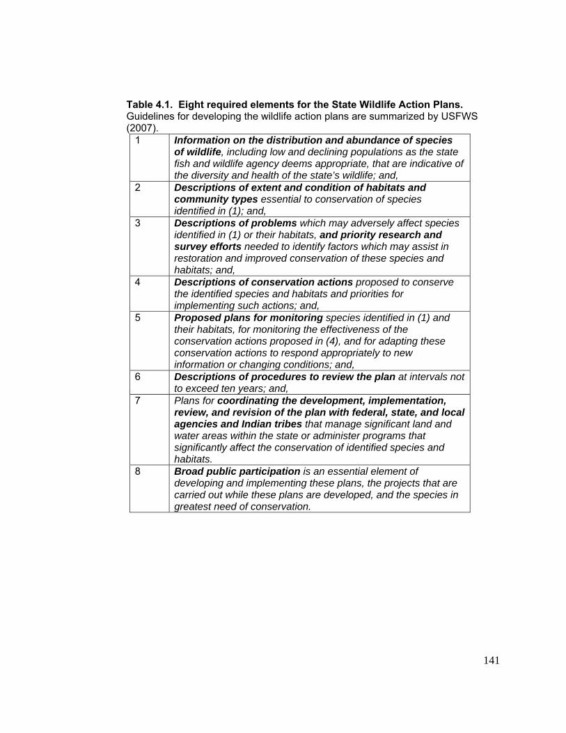
141
Guidelines for developing the wildlife action plans are summarized by USFWS
s appropriate, that are indicative of the diversity and health of the state’s wildlife; and,
Table 4.1. Eight required elements for the State Wildlife Action Plans.
(2007). 1 Information on the distribution and abundance of species
of wildlife, including low and declining populations as the state fish and wildlife agency deem
2 Descriptions of extent and condition of habitats and community types essential to conservation of species identified in (1); and,
3 Descriptions of problems which may adversely affect species identified in (1) or their habitats, and priority research and survey efforts needed to identify factors which may assist in restoration and improved conservation of these species and habitats; and,
4 Descriptions of conservation actions proposed to conserve the identified species and habitats and priorities for implementing such actions; and,
5 Proposed plans for monitoring species identified in (1) and their habitats, for monitoring the effectiveness of the conservation actions proposed in (4), and for adapting these conservation actions to respond appropriately to new information or changing conditions; and,
6 Descriptions of procedures to review the plan at intervals not to exceed ten years; and,
7 Plans for coordinating the development, implementation, review, and revision of the plan with federal, state, and local agencies and Indian tribes that manage significant land and water areas within the state or administer programs that significantly affect the conservation of identified species and habitats.
8 Broad public participation is an essential element of developing and implementing these plans, the projects that are carried out while these plans are developed, and the species in greatest need of conservation.
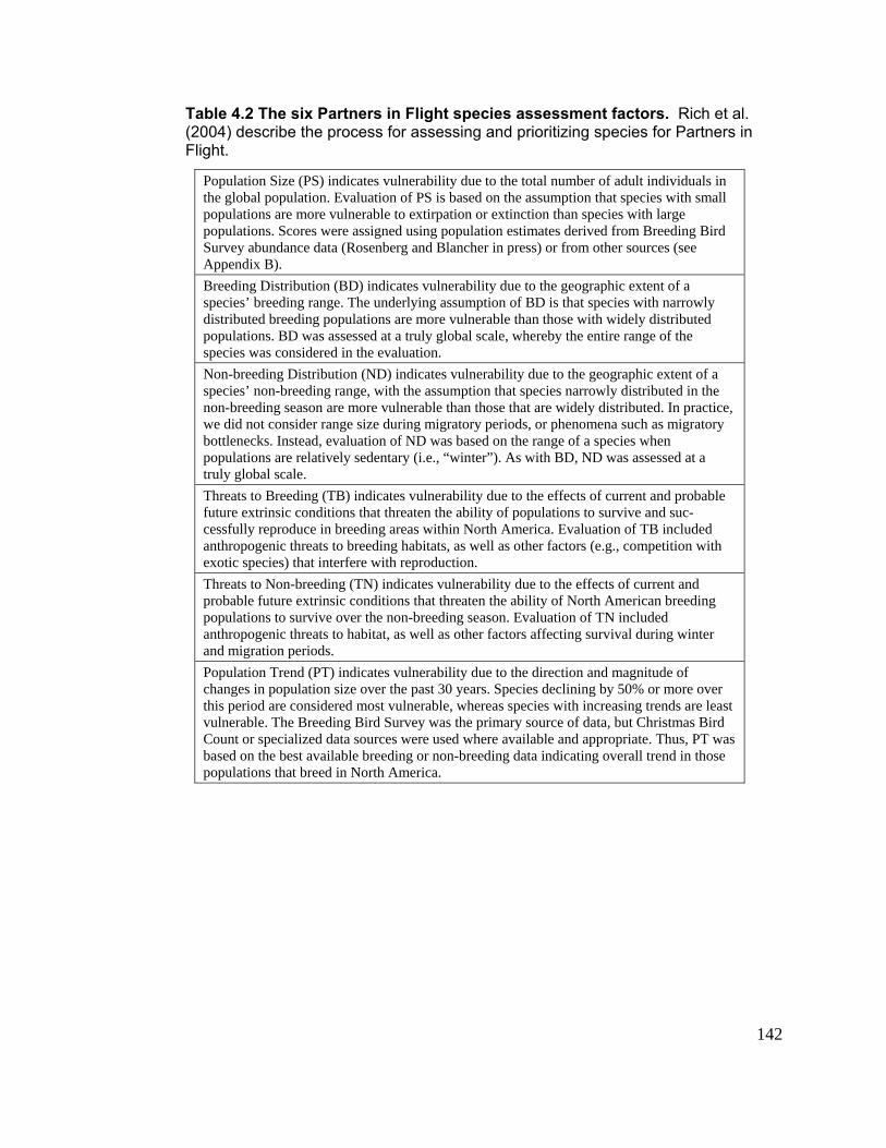
142
Table 4.2 The six Partners in Flight species assessment factors. Rich et al. (2004) describe the process for assessing and prioritizing species for Partners in Flight.
population. Evaluation of PS is based on the assumption that species with small ns
p lations Survey abuAppendix B
Population Size (PS) indicates vulnerability due to the total number of adult individuals in the global p latioopu
opu are more vulnerable to extirpation or extinction than species with large . Scores were assigned using population estimates derived from Breeding Birdndance data (Rosenberg and Blancher in press) or from other sources (see ).
Breeding D f a s ies’ bre rrowly distributed ributed po ulationsspecies was
istribution (BD) indicates vulnerability due to the geographic extent oeding range. The underlying assumption of BD is that species with nabreeding populations are more vulnerable than those with widely dist. BD was assessed at a trul
pec
p y global scale, whereby the entire range of the considered in the evaluation.
Non-breedi a species’ non e non-breedin ctice, we did not c during migratory periods, or phenomena such as migratory b eneckspopulations ssessed at a truly global
ng Distribution (ND) indicates vulnerability due to the geographic extent of-breeding range, with the assumption that species narrowly distributed in thg season are more vulnerable than those that are widely distributed. In praonsider range size
ottl . Instead, evaluation of ND was based on the range of a species when are relatively sedentary (i.e., “winter”). As with BD, ND was a scale.
T ats to B le future extrin nd suc-cessfully re d anthropoge exotic speci
hre reeding (TB) indicates vulnerability due to the effects of current and probabsic conditions that threaten the ability of populations to survive a
produce in breeding areas within North America. Evaluation of TB includenic threats to breeding habitats, as well as other factors (e.g., competition withes) that interfere with reproduction.
T ats to Np able fup lationsa ropogeand migrati
hrerob
on-breeding (TN) indicates vulnerability due to the effects of current and ture extrinsic conditions that threaten the ability of North American breeding
opunth
to survive over the non-breeding season. Evaluation of TN included nic threats to habitat, as well as other factors affecting survival during winter on periods.
Population changes in r this period vulnerable. g Bird Survey was the primary source of data, but Christmas Bird C nt or sp hus, PT was based on thpopulations
Trend (PT) indicates vulnerability due to the direction and magnitude of population size over the past 30 years. Species declining by 50% or more oveare considered most vulnerable, whereas species with increasing trends are least The Breedin
ou ecialized data sources were used where available and appropriate. Te best available breeding or non-breeding data indicating overall trend in those that breed in North America.
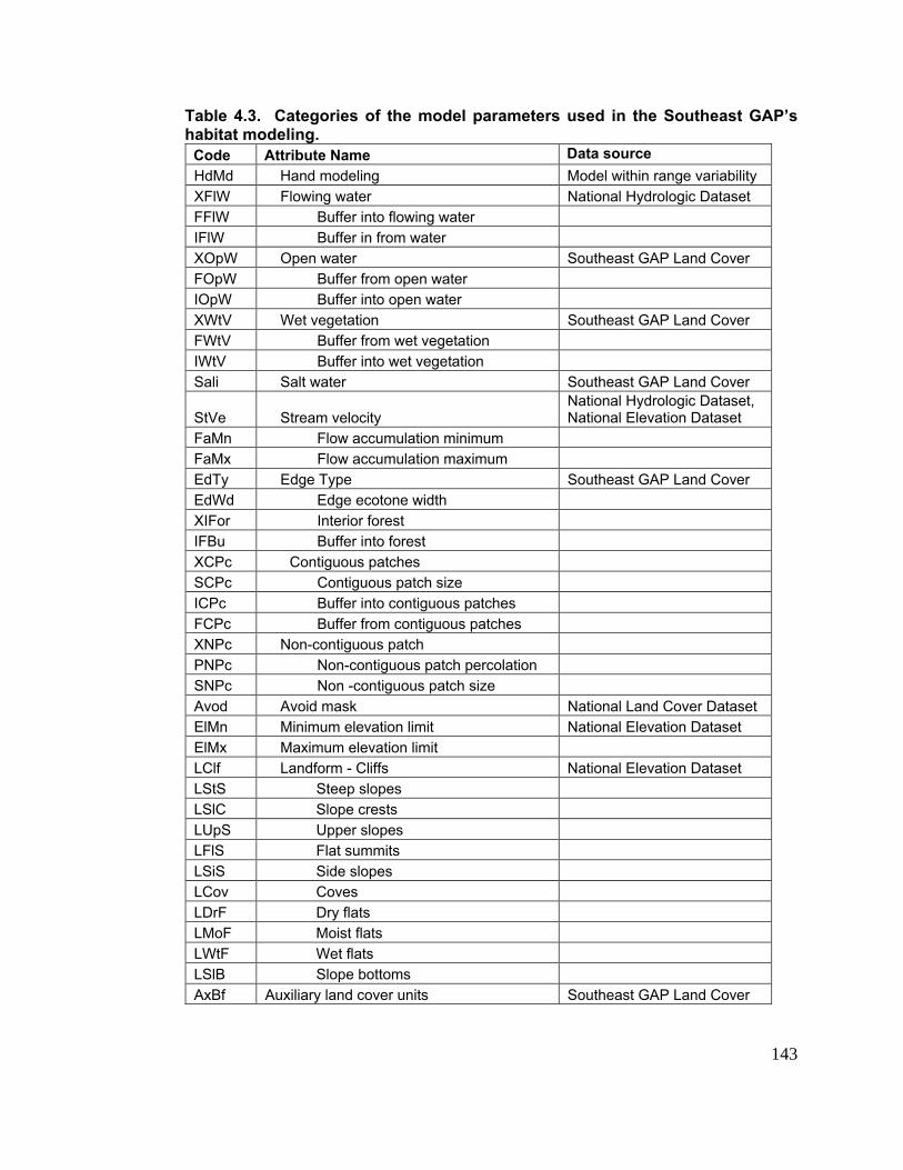
143
P’s
Attribute Name Data source
Table 4.3. Categories of the model parameters used in the Southeast GAhabitat modeling.
Code H y dMd Hand modeling Model within range variabilitX t FlW Flowing water National Hydrologic DataseFFlW Buffer into flowing water IFlW Buffer in from water X over OpW Open water Southeast GAP Land CFOpW Buffer from open water IOpW Buffer into open water X er WtV Wet vegetation Southeast GAP Land CovFWtV Buffer from wet vegetation IW tion tV Buffer into wet vegetaS r ali Salt water Southeast GAP Land Cove
St,
tVe Stream velocity National Hydrologic DataseNational Elevation Dataset
FaMn Flow accumulation minimum FaMx Flow accumulation maximum E er dTy Edge Type Southeast GAP Land CovEdWd Edge ecotone width XIFor Interior forest IFBu Buffer into forest XCPc Contiguous patches SCPc Contiguous patch size ICPc Buffer into contiguous patches FCPc Buffer from contiguous patches XNPc Non-contiguous patch P contiguous patch percolation NPc Non-SNPc Non -contiguous patch size Avod Avoid mask National Land Cover Dataset ElMn Minimum elevation limit National Elevation Dataset ElMx Maximum elevation limit LClf Landform - Cliffs National Elevation Dataset LS tS Steep slopes LSlC Slope crests LUpS Upper slopes LFlS Flat summits LSiS Side slopes LCov Coves LDrF Dry flats LMoF Moist flats LWtF Wet flats LSlB Slope bottoms AxBf Auxiliary land cover units Southeast GAP Land Cover
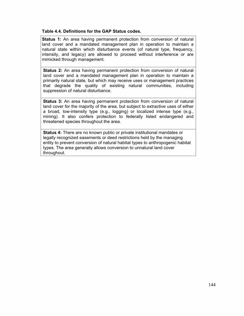
144
Tab
Sta manent protection from c tural land cover an anagement plan in operation to maintnatur e within which disturbance events (of natuinten nd legacy) are allowed to proceed withoutmimi rough
le 4.4. Definitions for the GAP Status codes.
tu An as 1: rea having perd a mandated m
onversion of naain a
ral type, frequency, al statsity, a interference or are cked th management.
Stat n ar ermanent protection from cland and plan in ope tion to maintain a prim tural ve uses or m agement practices that de f existing natural comsuppression of n
us 2: A ea having p onversion of natural cover a mandated management raarily na state, but which may recei an
degra the quality o munities, including atural disturbance.
Status 3: An area having permanent protection from cland cover for the major a, but subject to exta broad, low-intensity type (e.g., logging) or localizedmini also lly liste endangered and threa spec
onversion of natural ity of the are ractive uses of either
intense type (e.g., ng). It confers protection to federa dtened ies throughout the area.
Stat here rivate institutionlega gnize trictions held by the managing entity to prevent conversion of natur opogenic habitat types. The area generally allows conversion to unnatural land cover throughout.
us 4: Tlly reco
are no known public or pd easements or deed res
al mandates or
al habitat types to anthr
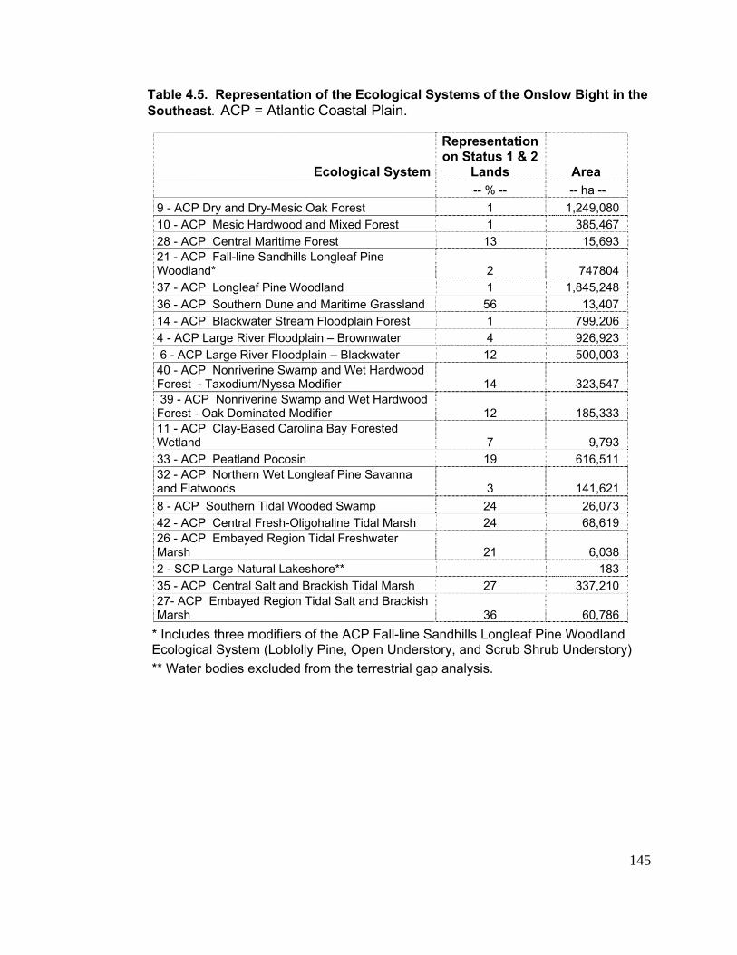
145
ystems of the Onslow Bight in the
Table 4.5. Representation of the Ecological SSoutheast. ACP = Atlantic Coastal Plain.
Ecological System
Representation on Status 1 & 2
Lands Area-- % -- -- ha --
9 - ACP Dry and Dry-Mesic Oak Forest 1 1,249,080 10 - ACP Mesic Hardwood and Mixed Forest 1 385,467 28 - ACP Central Maritime Forest 13 15,693 21 - ACP Fall-line Sandhills Longleaf Pine Woodland* 2 747804 37 - ACP Longleaf Pine Woodland 1 1,845,248 36 - ACP Southern Dune and Maritime Grassland 56 13,407 14 - ACP Blackwater Stream Floodplain Forest 1 799,206 4 - ACP Large River Floodplain – Brownwater 4 926,923 6 - ACP Large River Floodplain – Blackwater 12 500,003 40 - ACP Nonriverine Swamp and Wet Hardwood Forest - Taxodium/Nyssa Modifier 14 323,547 39 - ACP Nonriverine Swamp and Wet Hardwood Forest - Oak Dominated Modifier 12 185,333 11 - ACP Clay-Based Carolina Bay Forested Wetland 7 9,793 33 - ACP Peatland Pocosin 19 616,511 32 - ACP Northern Wet Longleaf Pine Savanna and Flatwoods 3 141,621 8 - ACP Southern Tidal Wooded Swamp 24 26,073 42 - ACP Central Fresh-Oligohaline Tidal Marsh 24 68,619 26 - ACP Embayed Region Tidal Freshwater Marsh 21 6,038 2 - SCP Large Natural Lakeshore** 183 35 - ACP Central Salt and Brackish Tidal Marsh 27 337,210 27- ACP Embayed Region Tidal Salt and Brackish Marsh 36 60,786
* Includes three modifiers of the ACP Fall-line Sandhills Longleaf Pine Woodland Ecological System (Loblolly Pine, Open Understory, and Scrub Shrub Understory) ** Water bodies excluded from the terrestrial gap analysis.
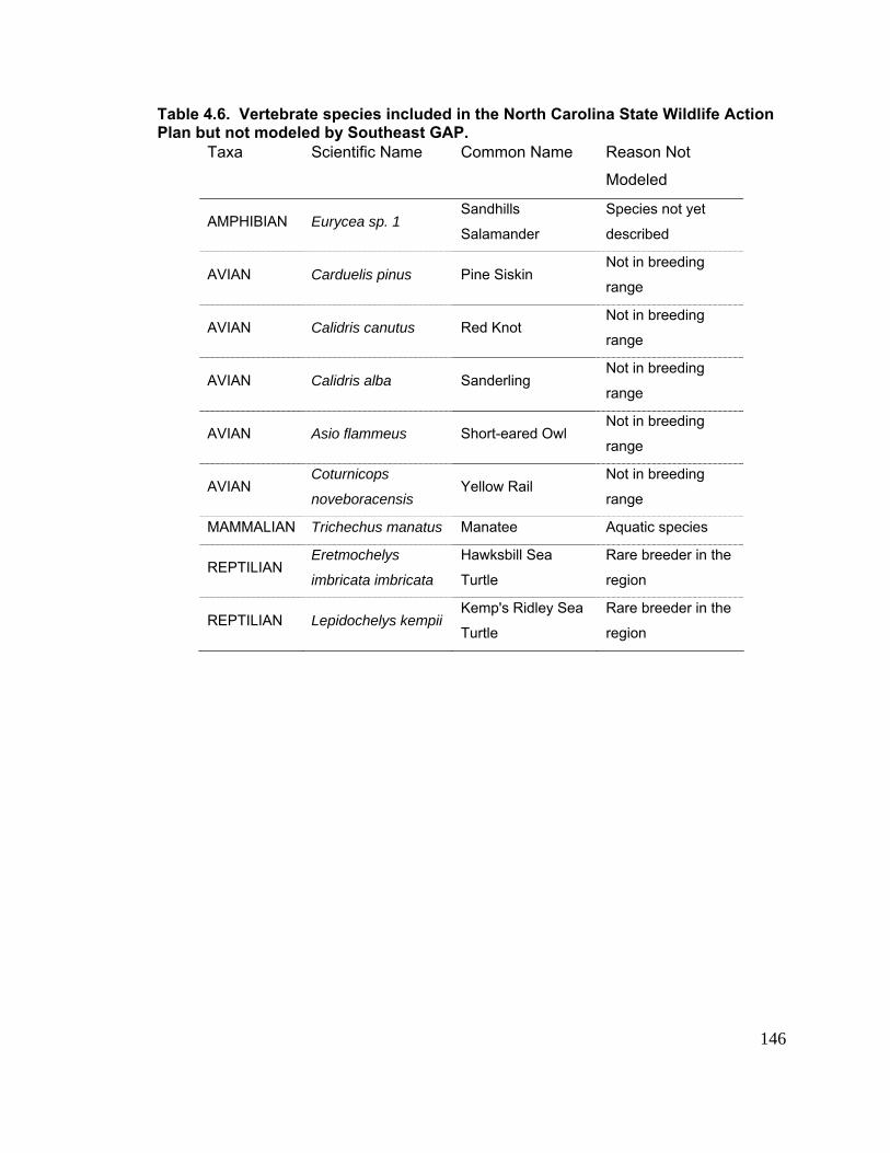
146
TaPla
Taxa Scientific Name Common Name Reason Not
d
AMPHIBIAN Eurycea sp.Salamander
ecies not
scribed
ble 4.6. Vertebrate species included in the North Carolina State Wildlife Action n but not modeled by Southeast GAP.
Modele
Sp 1
Sandhills yet
de
AVIAN Carduelis pinus Pine Siskin Not in breedi
range
ng
AVIAN Calidris canutus Red Knot Not in breeding
range
AVIAN Calidris alba Sanderling Not in breeding
range
AVIAN Asio flammeus Short-eared Owl Not in breedin
range
g
AVIAN Coturnicops
noveboracensis Yellow Rail
Not in breedin
range
g
MAMMALIAN Trichechus manatus Manatee Aquatic species
REPTILIAN imbricata imbricata Turtle
Eretmochelys Hawksbill Sea Rare breeder
region
in the
REPTILIAN Lepidochelys kempii Kemp's Ridley Sea Rare breeder i
region
Turtle
n the
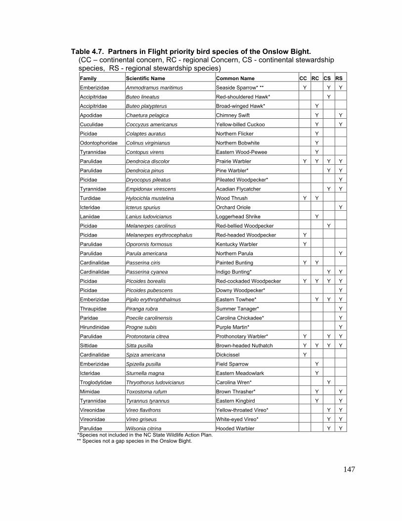
147
ncern, CS - continental stewardship spec S - regio pecFamily Scientific Name Common Name RC CS RS
Table 4.7. Partners in Flight priority bird species of the Onslow Bight. (CC – continental concern, RC - regional Co
ies, R nal stewardship s ies) CC
Emberizidae Ammodramus maritimus Seaside Sparrow* ** Y Y Y
Accip eo ldered Hawk* Y itridae But lineatus Red-shou
Accipitridae Buteo platypteru Hawk* Y s Broad-winged
Apodidae Chaetura pelagica Chimney Swift Y Y
Cucu Coccy Cuckoo Y Y lidae zus americanus Yellow-billed
Picidae Colaptes auratus Northern Flicker Y
Odonto Colinus vir white phoridae ginianus Northern Bob Y
Tyran Conto ood-Pewee Y nidae pus virens Eastern W
Parulidae Dendroica discolor Prairie Warbler Y Y Y Y
Parul Dend r* Y Y idae roica pinus Pine Warble
Picidae Dryocopus pileatus Pileated Woodpecker* Y
Tyrannidae Empidonax virescens Acadian Flycatcher Y Y
Turdi Hyloc Y Y dae ichla mustelina Wood Thrush
Icteridae Icterus spurius Orchard Oriole Y
Laniid Laniu Shrike ae s ludovicianus Loggerhead Y
Picidae Melan Red-bellied Woodpecke Y erpes carolinus r
Picida n odpecke e Mela erpes erythrocephalus Red-headed Wo r Y
Parulidae Oporornis formosus Kentucky Warbler Y
Parul rul Y idae Pa a americana Northern Parula
Cardinalidae Passe ed Bunting Y Y rina ciris Paint
Cardinalidae Passerina cyanea Y Indigo Bunting* Y
Picida coid oodpecker Y Y Y Y e Pi es borealis Red-cockaded W
Picidae Picoides pubescens y Woodpecker* Y Down
Emberizidae Pipilo erythrophthalmus Eastern Towhee* Y Y Y
Thraupidae Piranga rubra Summer Tanager* Y
Paridae Poecile carolinensis Carolina Chickadee* Y
Hirundinidae Progne subis Purple Martin* Y
Parulidae Protonotaria citrea Prothonotary Warbler* Y Y Y
Sittidae Sitta pusilla Brown-headed Nuthatch Y Y Y Y
Cardinalidae Spiza americana Dickcissel Y
Emberizidae Spizella pusilla Field Sparrow Y
Icteridae Sturnella magna Eastern Meadowlark Y
Troglodytidae Thryothorus ludovicianus Carolina Wren* Y
Mimidae Toxostoma rufum Brown Thrasher* Y Y
Tyrannidae Tyrannus tyrannus Eastern Kingbird Y Y
Vireonidae Vireo flavifrons Yellow-throated Vireo* Y Y
Vireonidae Vireo griseus White-eyed Vireo* Y Y
Parulidae Wilsonia citrina Hooded Warbler Y Y *Species not included in the NC State Wildlife Action Plan. ** Species not a gap species in the Onslow Bight.

148
of Ecga ion. The Southeast GAP Status map from 2001 was used to summarize both the 1 acreages by cat de Change tive to the 9 to l. * Includes three modifiers of the ACP Fall-line S Woodland Ecological System (Lobl** Small and large river floodplain systems w d in the prelimin rySo n GA*** Carolina Bay P sin combined tland Pocosin in the preliminary Southeastern Gap Analysis. **** dies m the terrestria
Table 4.8. Land cover scorecard. Changes in the extent and representationological Systems in the Onslow Bight. Ecological Systems in bold are considered ps at the 10% threshold for the Southeast Reg
992 and 2001 status (Statusegories are fined in Table 4.4). is calculated rela 19 2 ta
andhills Longleaf Pine olly Pine, Open Understory, and Scrub Shrub Understory).
ere combine a utheaster P.
eatland Poco with ACP Pea
Water bo excluded fro l gap analysis.
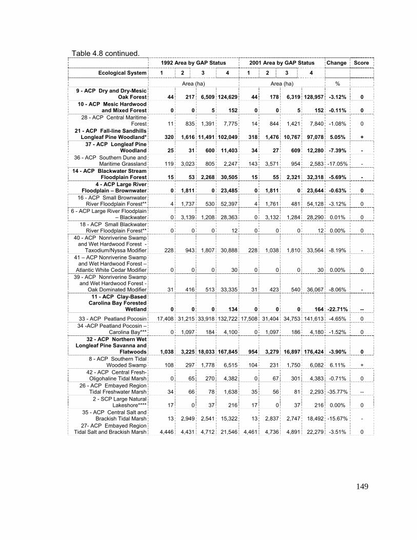
149
Table 4.8 continued. 1992 Area by GAP Status 2001 Area by GAP Status Change Score
Ecological System 1 2 3 4 1 2 3 4
Area (ha) Area (ha) % 9 - ACP Dry and Dry-Mesic
Oak Forest 44 217 6,509 124,629 44 178 6,319 128,957 -3.12% 0 10 - ACP Mesic Hardwood
and Mixed Forest 0 0 5 152 0 0 5 152 -0.11% 0 28 - ACP Central Maritime
Forest 11 835 1,391 7,775 14 844 1,421 7,840 -1.08% 0 21 - ACP Fall-line Sandhills
% + Longleaf Pine Woodland* 320 1,616 11,491 102,049 318 1,476 10,767 97,078 5.0537 - ACP Longleaf Pine
Woodland 25 31 600 11,403 34 27 609 12,280 -7.39% - 36 - ACP Southern Dune and
Maritime Grassland 119 3,023 805 2,247 143 3,571 954 2,583 -17.05% - 14 - ACP Blackwater Stream
Floodplain Forest 15 53 2,268 30,505 15 55 2,321 32,318 -5.69% - 4 - ACP Large River
Floodplain – Brownwater 0 1,811 0 23,485 0 1,811 0 23,644 -0.63% 0 16 - ACP Small Brownwater
River Floodplain Forest** 4 1,737 530 52,397 4 1,761 481 54,128 -3.12% 0 6 - ACP Large River Floodplain
– Blackwater 0 3,139 1,208 28,363 0 3,132 1,284 28,290 0.01% 0 18 - ACP Small Blackwater
River Floodplain Forest** 0 0 0 12 0 0 0 12 0.00% 0 40 - ACP Nonriverine Swamp
and Wet Hardwood Forest - Taxodium/Nyssa Modifier 228 943 1,807 30,888 228 1,038 1,810 33,564 -8.19% -
41 – ACP Nonriverine Swamp and Wet Hardwood Forest –
Atlantic White Cedar Modifier 0 0 0 30 0 0 0 30 0.00% 0 39 - ACP Nonriverine Swamp
and Wet Hardwood Forest - Oak Dominated Modifier 31 416 513 33,335 31 423 540 36,067 -8.06% -
11 - ACP Clay-Based Carolina Bay Forested
Wetland 0 0 0 134 0 0 0 164 -22.71% --
33 - ACP Peatland Pocosin 17,408 31,215 33,918 132,722 17,508 31,404 34,753 141,613 -4.65% 0 34 -ACP Peatland Pocosin –
Carolina Bay*** 0 1,097 184 4,100 0 1,097 186 4,180 -1.52% 0 32 - ACP Northern Wet
Longleaf Pine Savanna and Flatwoods 1,038 3,225 18,033 167,845 954 3,279 16,897 176,424 -3.90% 0
8 - ACP Southern Tidal Wooded Swamp 108 297 1,778 6,515 104 231 1,750 6,082 6.11% +
42 - ACP Central Fresh-Oligohaline Tidal Marsh 0 65 270 4,382 0 67 301 4,383 -0.71% 0
26 - ACP Embayed Region Tidal Freshwater Marsh 34 66 78 1,638 35 56 81 2,293 -35.77% --
2 - SCP Large Natural Lakeshore**** 17 0 37 216 17 0 37 216 0.00% 0
35 - ACP Central Salt and Brackish Tidal Marsh 13 2,949 2,541 15,322 13 2,837 2,747 18,492 -15.67% -
27- ACP Embayed Region Tidal Salt and Brackish Marsh 4,446 4,431 4,712 21,546 4,461 4,736 4,891 22,279 -3.51% 0
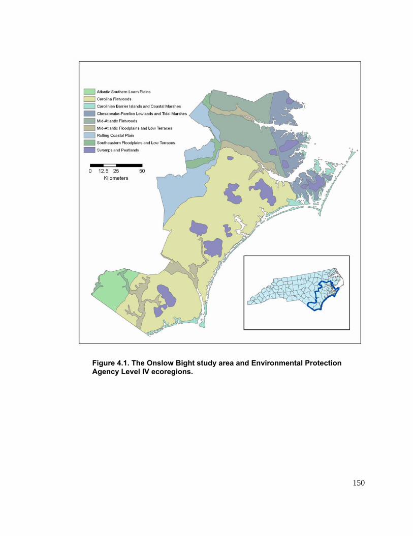
150
Figu ns Bi a n nv m l c ecor ion
re 4.1. The O low ght study rea a d E iron enta Prote tion
Agency Level IV eg s.
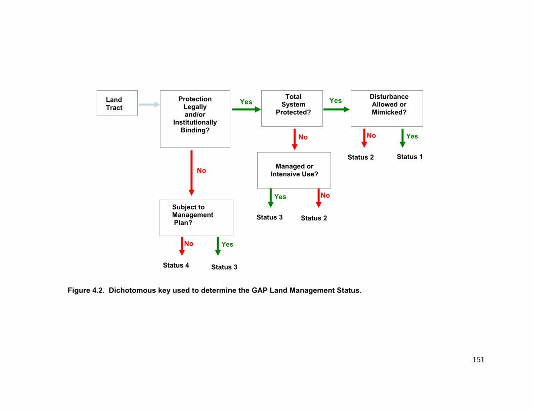
151
Figure 4.2. Dichotomous ke sed to determine the GAP Land Management Status.
y u
No Yes
Yes
No
No
Status 1 Status 2
Status 2 Status 3
Status 3 s 4 Statu
Disturbance Allowed or Mimicked?
SM P
ubject to anagement lan?
Total System
Protected?
Protection Legally and/or
stitutionally Binding?
In
Land Tract
Managed or Intensive Use?
Yes
Yes
No
No
Yes
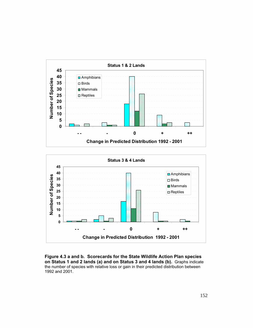
152
Status 1 & 2 Lands
05
1015202530354045
- - - 0 + ++
hange in Predicted Distribution 1992 - 2
Num
ber o
f Spe
cies
AmphibiansBirdsMammalsReptiles
C 001
Status 3 & 4 Lands
05
1015202530354045
- - - 0 + ++
Change in Predicted Distribution 1992 - 2001
Num
ber o
f Spe
cies
AmphibiansBirdsM alsammRe sptile
Figure 4.3 a and b. Scorecards for the State Wildlife Action Plan species on Status 1 and 2 lands (a) and on Status 3 and 4 lands (b). Graphs indicate the number of species with relative loss or gain in their predicted distrib ween 1992 and 2001.
ution bet
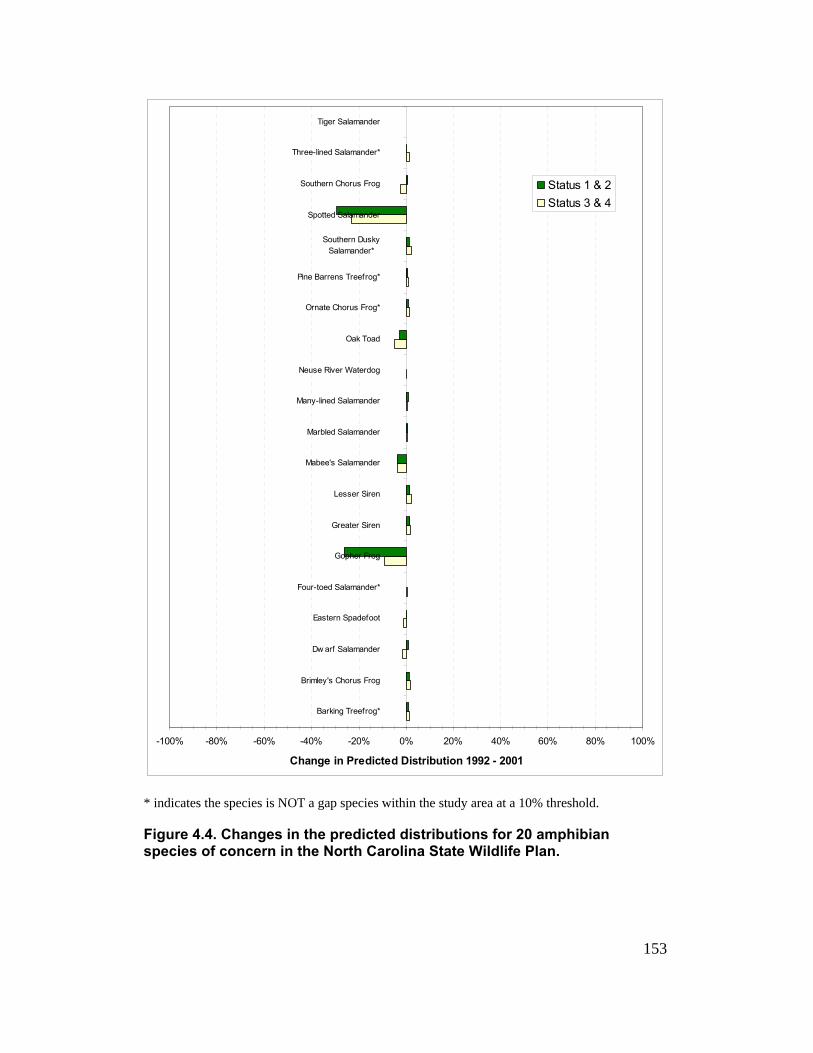
-100% -80% -60% -40% -20% 0% 20% 40% 60% 80% 100%
Barking Treefrog*
Brimley's Chorus Frog
Dw arf Salamander
Eastern Spadefoot
Four-toed Salamander*
Gopher Frog
Greater Siren
Lesser Siren
Mabee's Salamander
Marbled Salamander
Many-lined Salamander
Neuse River Waterdog
Oak Toad
Ornate Chorus Frog*
Pine Barrens Treefrog*
Southern DuskySalamander*
Spotted Salamander
Southern Chorus Frog
Three-lined Salamander*
Tiger Salamander
Change in Predicted Distribution 1992 - 2001
Status 1 & 2Status 3 & 4
* indicates the species is NOT a gap species within the study area at a 10% threshold. Figure 4.4. Changes in the predicted distributions for 20 amphibian species of concern in the North Carolina State Wildlife Plan.
153
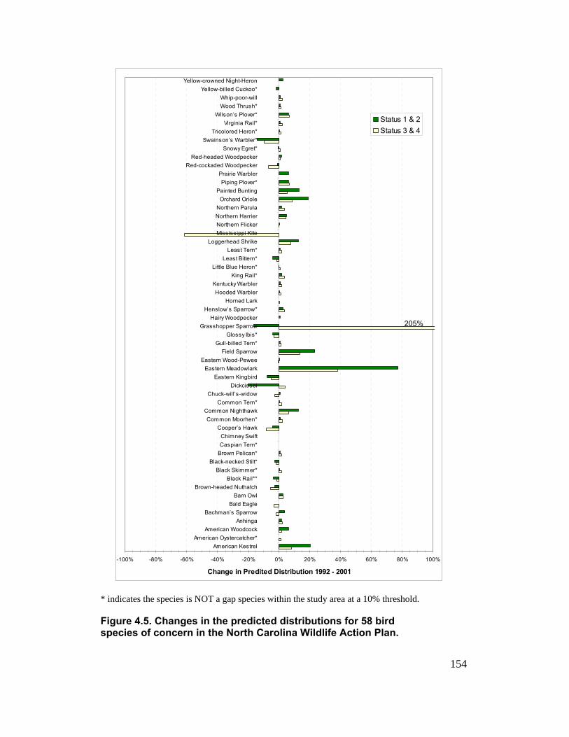
154
old. Figure 4.5. Changes in the predicted distributions for 58 bird species of concern in the North Carolina Wildlife Action Plan.
* indicates the species is NOT a gap species within the study area at a 10% thresh
-100% -80% -60% -40% -20% 0% 20% 40% 60% 80% 100%
American KestrelAmerican Oystercatcher*
American WoodcockAnhinga
Bachman’s SparrowBald Eagle
Barn OwlBrown-headed Nuthatch
Black Rail**Black Skimmer*
Black-necked Stilt*Brown Pelican*Caspian Tern*Chimney Swift
Cooper’s HawkCommon Moorhen*
Common NighthawkCommon Tern*
Chuck-will’s-widowDickcissel
Eastern KingbirdEastern Meadowlark
Eastern Wood-PeweeField Sparrow
Gull-billed Tern*Glossy Ibis*
Grasshopper SparrowHairy Woodpecker
Henslow’s Sparrow*Horned Lark
Hooded WarblerKentucky Warbler
King Rail*Little Blue Heron*
Least Bittern*Least Tern*
Loggerhead ShrikeMississippi KiteNorthern FlickerNorthern HarrierNorthern Parula
Orchard OriolePainted Bunting
Piping Plover*Prairie Warbler
Red-cockaded WoodpeckerRed-headed Woodpecker
Snowy Egret*Swainson’s Warbler*
Tricolored Heron*Virginia Rail*
Wilson’s Plover*Wood Thrush*Whip-poor-will
Yellow-billed Cuckoo*Yellow-crowned Night-Heron
Change in Predited Distribution 1992 - 2001
Status 1 & 2Status 3 & 4
205%
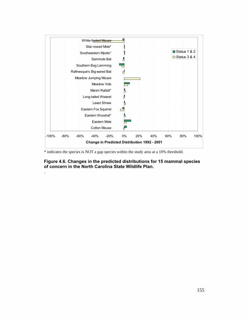
155
-100% -80% -60% -40% -20% 0% 20% 40% 60% 80% 100%
Cotton Mouse
Eastern Mole
Eastern Woodrat*
Eastern Fox Squirrel
Least Shrew
Long-tailed Weasel
Marsh Rabbit*
Meadow Vole
Meadow Jumping Mouse
Rafinesque's Big-eared Bat
Southern Bog Lemming
Seminole Bat
Southeastern Myotis*
Star-nosed Mole*
White-footed Mouse
Change in Predicted Distribution 1992 - 2001
Status 1 & 2Status 3 & 4
* indicates the species is NOT a gap species within the study area at a 10% threshold. Figure 4.6. Changes in the predicted distributions for 15 mammal species of concern in the North Carolina State Wildlife Plan. .
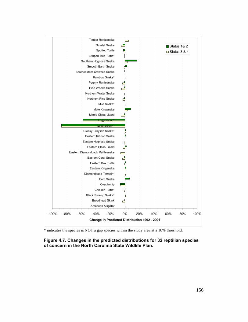
-100% -80% -60% -40% -20% 0% 20% 40% 60% 80% 100%
American Alligator
Broadhead Skink
Black Swamp Snake*
Chicken Turtle*
Coachwhip
Corn Snake
Diamondback Terrapin*
156
Eastern Kingsnake
Eastern Box Turtle
Eastern Coral Snake
Eastern Diamondback Rattlesnake
Eastern Glass Lizard
Eastern Hognose Snake
Eastern Ribbon Snake
Glossy Crayfish Snake*
Leatherback*
Loggerhead*
Mimic Glass Lizard
Mole Kingsnake
Mud Snake*
Northern Pine Snake
Northern Water Snake
Pine Woods Snake
Pygmy Rattlesnake
Rainbow Snake*
Southeastern Crowned Snake
Smooth Earth Snake
Southern Hognose Snake
Striped Mud Turtle*
Spotted Turtle
Scarlet Snake
Timber Rattlesnake
Change in Predicted Distribution 1992 - 2001
Status 1& 2Status 3 & 4
* indicates the species is NOT a gap species within the study area at a 10% threshold. Figure 4.7. Changes in the predicted distributions for 32 reptilian species of concern in the North Carolina State Wildlife Plan.
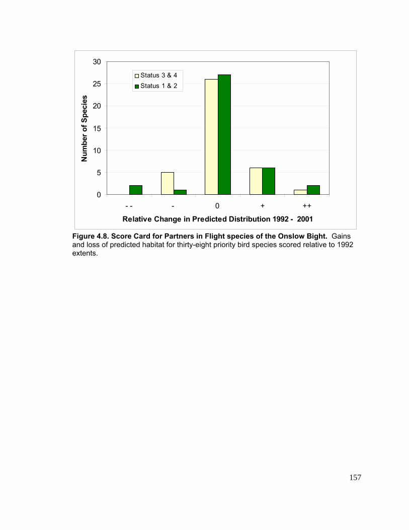
0
5
10
15
20
25
30
- - - 0 + ++
Relative Change in Predicted Distribution 1992 - 2001
Num
ber o
f Spe
cies
Status 3 & 4Status 1 & 2
Figure 4.8. Score Card for Partners in Flight species of the Onslow Bight. Gains and loss of predicted habitat for thirty-eight priority bird species scored relative to 1992 extents.
157
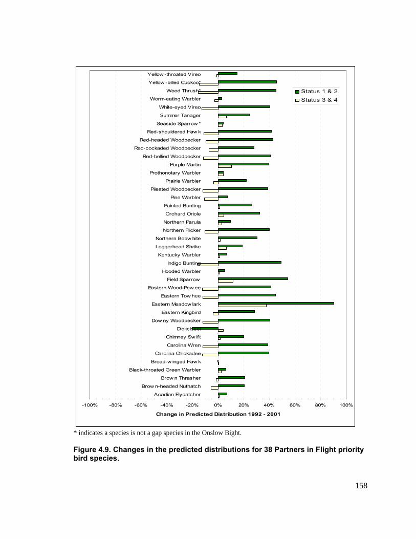
158
-100% -80% -60% -40% -20% 0% 20% 40% 60% 80% 100%
Acadian Flycatcher
Brow n-headed Nuthatch
Brow n Thrasher
Black-throated Green Warbler
Broad-w inged Haw k
Carolina Chickadee
Carolina Wren
Chimney Sw ift
Dickcissel
Dow ny Woodpecker
Eastern Kingbird
Eastern Meadow lark
Eastern Tow hee
Eastern Wood-Pew ee
Field Sparrow
Hooded Warbler
Indigo Bunting
Kentucky Warbler
Loggerhead Shrike
Northern Bobw hite
Northern Flicker
Northern Parula
Orchard Oriole
Painted Bunting
Pine Warbler
Pileated Woodpecker
Prairie Warbler
Prothonotary Warbler
Purple Martin
Red-bellied Woodpecker
Red-cockaded Woodpecker
Red-headed Woodpecker
Red-shouldered Haw k
Seaside Sparrow *
Summer Tanager
White-eyed Vireo
Worm-eating Warbler
Wood Thrush*
Yellow -billed Cuckoo*
Yellow -throated Vireo
Change in Predicted Distribution 1992 - 2001
Status 1 & 2Status 3 & 4
* indicates a species is not a gap species in the Onslow Bight. Figure 4.9. Changes in the predicted distributions for 38 Partners in Flight priority bird species.
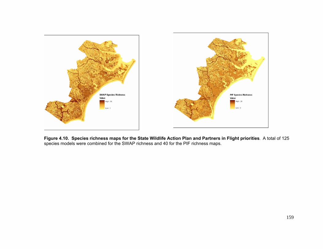
159
Figure 4.10. Species richness maps for the State Wildlife Action Plan and Partners in Flight priorities. A total of 125 sp s dels were combined for the SWAP richness and 40 for the PIF richness maps.
ecie mo
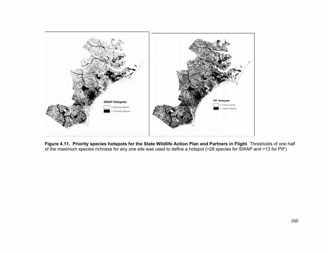
160
es for SWAP and >13 for PIF) Figure 4.11. Priority species hotspots for the State Wildlife Action Plan and Partners in Flight. Thresholds of one half of the maximum species richness for any one site was used to define a hotspot (>28 speci
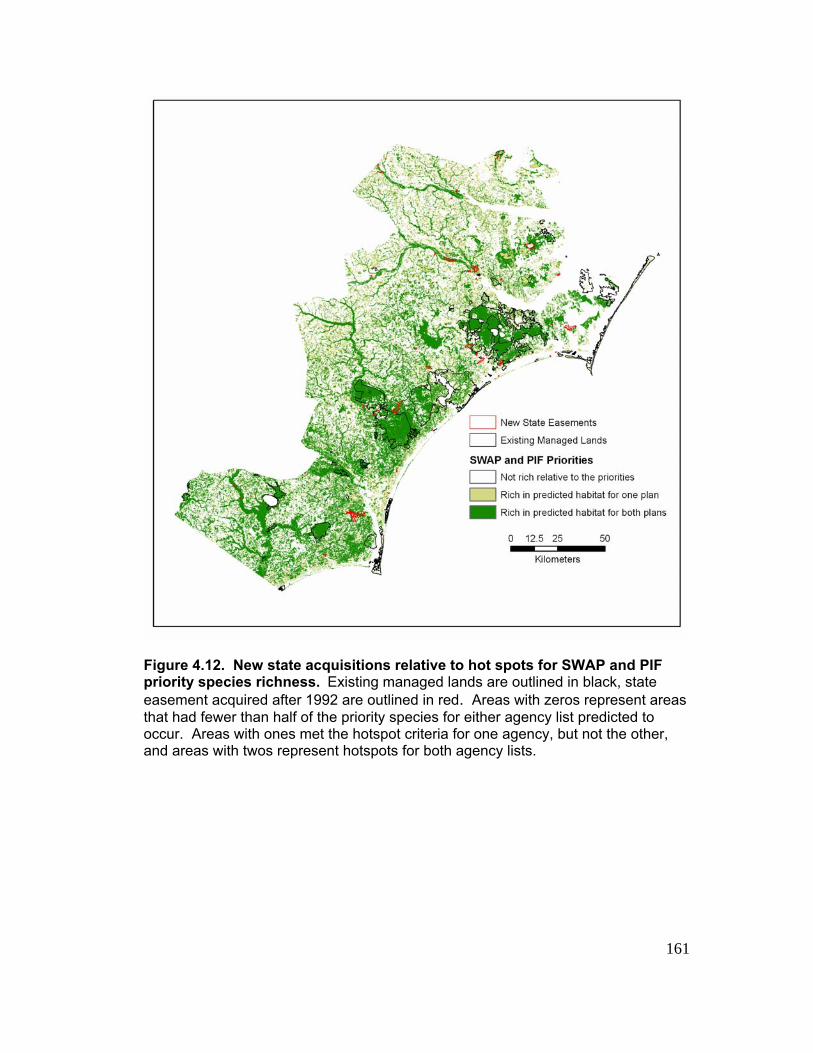
Figure 4.12. New state acquisitions relative to hot spots for SWAP and PIF priority species richness. Existing managed lands are outlined in black, state easement acquired after 1992 are outlined in re as with zeros represent areas that had fewer than half of the priority species fo r agency list predicted to occur. Areas with ones met the hotspot criteria agency, but not the other, and areas with twos represent hotspots for both y lists.
d. Arer eithe
for one agenc
161
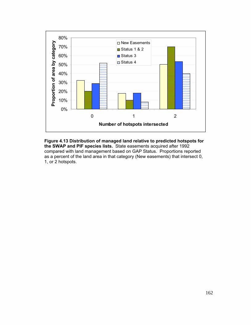
0%
10%
20%
30%
40%
50%
60%
70%
80%
0 1 2
Number of hotspots intersected
Prop
ortio
n of
are
a by
cat
egor
y New EasementsStatus 1 & 2Status 3Status 4
Figure 4.13 Distribution of managed land relative to predicted hotspots for the SWAP and PIF species lists. State easements acquired after 1992 compared with land management based on GAP Status. Proportions reported as a percent of the land area in that category (New easements) that intersect 0, 1, or 2 hotspots.
162

163
APPENDICES
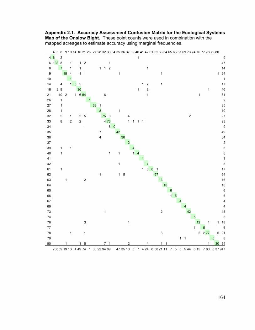
164
Appendix 2.1. Accuracy Assessment Confusion Matrix for the Ecological Systems Map of the Onslow Bight. These point counts were used in combination with the mapped acreages to estimate accuracy using marginal frequencies.
4 6 8 9 10 14 16 21 26 27 28 32 33 34 35 36 37 39 40 41 42 61 62 63 64 65 66 67 69 73 74 76 77 78 79 80
4 6 2 1 96 133 8 1 1 2 1 478 7 1 1 1 1 2 1 149 15 4 1 1 1 1 1 24
10 1 114 4 1 3 5 1 2 1 1716 2 9 30 1 3 1 4621 10 2 1 6 54 6 1 1 8126 1 1 227 1 33 1 3528 1 8 1 1032 5 1 2 5 75 3 4 2 9733 8 2 2 4 73 1 1 1 1 9334 1 8 0 935 7 42 4936 4 30 3437 2 239 1 1 4 640 1 1 1 1 4 841 1 142 1 7 861 1 1 6 8 1 1762 1 1 5 57 6463 1 2 13 1664 10 1065 6 666 1 5 667 4 469 4 473 1 2 42 4574 5 576 3 1 12 1 1 1877 1 5 678 1 1 3 2 2 77 5 9179 1 1 6 880 1 1 5 7 1 2 4 1 1 1 30 54
73559 19 13 4 49 74 1 33 22 94 89 47 35 10 6 7 4 24 8 58 21 11 7 5 5 5 44 6 15 7 80 6 37 947
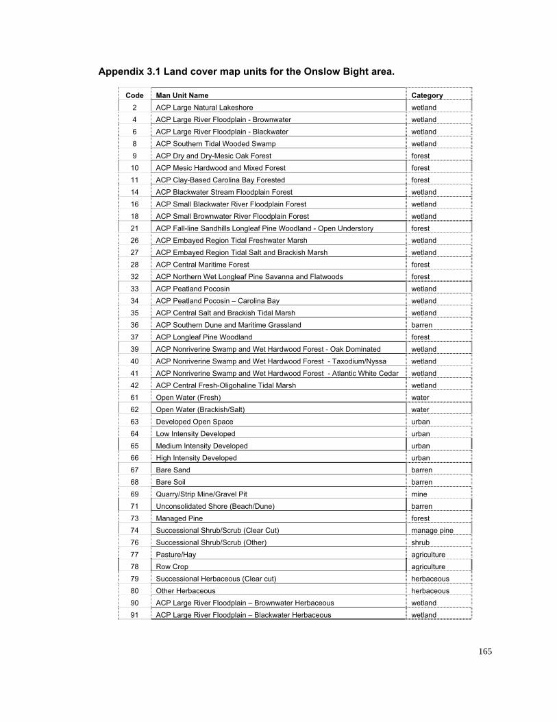
165
Category
Appendix 3.1 Land cover map units for the Onslow Bight area.
Code Man Unit Name 2 ACP Large Natural Lakeshore wetland 4 ACP Large River Floodplain - Brownwater wetland 6 ACP Large River Floodplain - Blackwater w tland e8 ACP Southern Tidal Wooded Sw m w tland a p e9 ACP r M s O st forest Dry and D y- e ic ak Fore
10 AC M s H rd o d i o forest P e ic a w od an M xed F rest 11 ACP Clay a ed ol a a F e e forest -B s Car in B y or st d 14 AC c er tr F o l n Forest w tlandP Bla kwat S eam lo dp ai e 16 ACP Small Blackwate iv r o p in w tlanr R e Fl od la Forest e d 18 AC S all w e w tlandP m Bro nwat r River Floodplain Forest e 21 AC F ll e d s o l f in W o a d O e t y forest P a -lin San hill L ng ea P e o dl n - pen Und rs or 26 AC E b y Re n d Fr w te M rsh w tlandP m a ed gio Ti al esh a r a e 27 ACP y R gi nd c s M rs tland Emba ed e on Tidal Salt a Bra ki h a h we 28 ACP n l a forest Ce tra M ritime Forest 32 AC No rn W t ngl t ods forest P rthe e Lo eaf Pine Savanna and Fla wo33 AC P a n Pocosin w tlandP e tla d e 34 AC P a n Poc n C r na w tlandP e tla d osi – a oli Bay e 35 AC C n l al n B c s T al M s w tlandP e tra S t a d ra ki h id ar h e 36 AC S u e D M ritime Grassland barren P o th rn une and a37 AC L n a Pi oo d forest P o gle f ne W dlan39 AC N n e ne w m a d Hard o F s O k o i te w tlandP o riv ri S a p n Wet w od ore t - a D m na d e 40 AC N n e ne w m a d W Hard o ores x i m yssa w tlandP o riv ri S a p n et w od F t - Ta od u /N e 41 AC N n e ne w m a d Hard o F w tlandP o riv ri S a p n Wet w od orest - Atlantic White Cedar e 42 AC C n l resh-Oligohaline Tidal Marsh w tlandP e tra F e 61 Op W r re h w teen ate (F s ) a r 62 Op a r (Bra i / l w teen W te ck sh Sa t) a r 63 De l e O en p c urban ve op d p S a e 64 Low Intensity e l e urban D ve op d65 y Developed urban Medium Intensit66 Hig I t ah ntensi y Developed urb n 67 Bare Sand r ba ren68 Ba Soil re barren 69 Qu r in minar y/Strip M e/Gravel Pit e 71 Un ns a d o e h e barren co olid te Sh re (B ac /Dun ) 73 Ma d in forest nage P e74 Succ a h b/S u C Cut manage pine ession l S ru cr b ( lear ) 76 Succession Oal Shrub/Scrub ( ther) shrub 77 Pasture/Hay agriculture 78 Row Crop agriculture 79 Successional Herbaceous (Clear cut) herbaceous 80 Other Herbaceous herbaceous 90 ACP Large River Floodplain – Brownwater Herbaceous wetland 91 ACP Large River Floodplain – Blackwater Herbaceous wetland
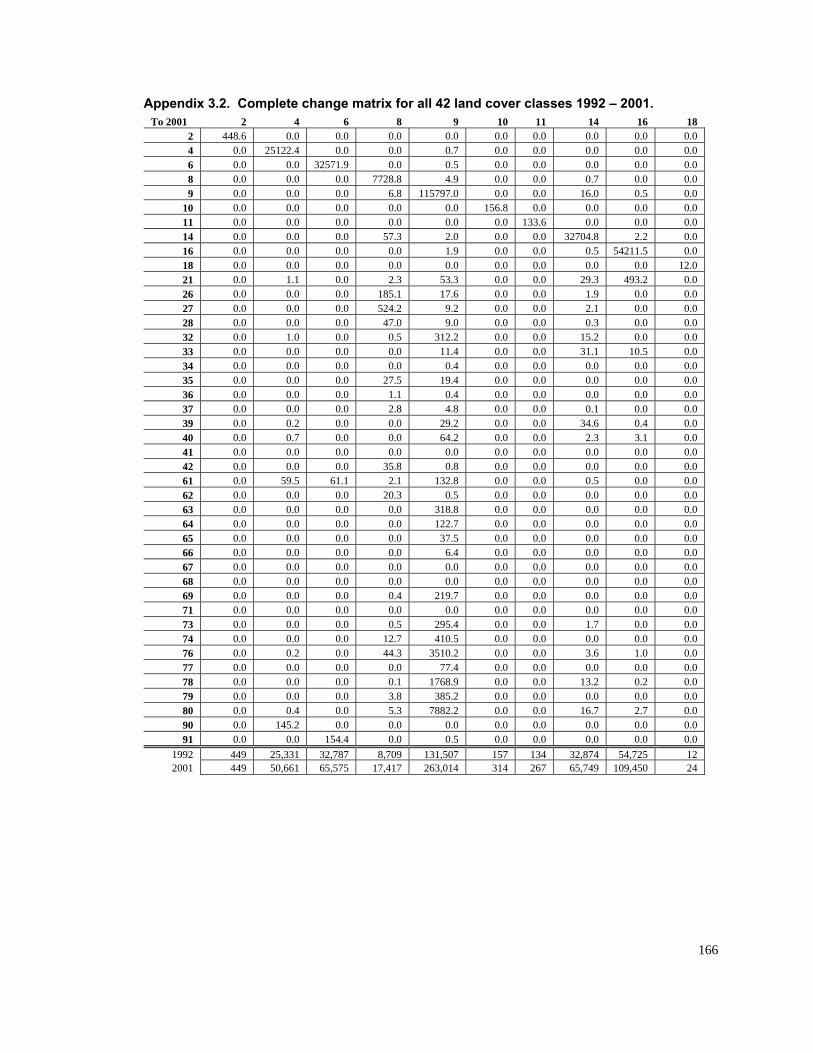
166
992 – 2001. To 2001 2 4 6 8 9 10 11 14 16 18
4 0.0 0.0 0.0 0.0 0.0 0.0 0.0
Appendix 3.2. Complete change matrix for all 42 land cover classes 1
2 48.6 0.0 0.0 4 0.0 0.7 0.0 0.0 0.0 0 0.0 0.0 25122.4 0.0 0.6 0.0 0.5 0.0 0.0 0.0 0 0.0 0.0 0.0 32571.9 0.8 4.9 0.0 0.0 0.7 0 0.0 0.0 0.0 0.0 7728.8 0.9 5797.0 0.0 0.0 16.0 5 0.0 0.0 0.0 0.0 6.8 11 0.
10 0.0 156.8 0.0 0.0 0 0.0 0.0 0.0 0.0 0.0 0.11 0.0 0.0 133.6 0.0 0.0 0.0 0.0 0.0 0.0 0.014 2.0 0.0 0.0 32704.8 2.2 0.0 0.0 0.0 0.0 57.3 1 1.9 0.0 0.0 0.5 1.5 0.0 6 0.0 0.0 0.0 0.0 54211 0.0 0.0 0.0 0.0 0.0 12.0 8 0.0 0.0 0.0 0.0 2 53.3 0.0 0.0 29.3 2 0.0 1 0.0 1.1 0.0 2.3 493.2 6 0.0 0.0 1.9 0 0.0 6 0.0 0.0 0.0 185.1 17. 0.2 0.0 0.0 2.1 0 0.0 7 0.0 0.0 0.0 524.2 9.2 0.2 0.0 0.0 0.3 0 0.0 8 0.0 0.0 0.0 47.0 9.0 0.3 15.2 0.0 0.0 2 0.0 1.0 0.0 0.5 312.2 0.0 0.0 3 0.0 0.0 31.1 5 0.0 3 0.0 0.0 0.0 0.0 11.4 10.3 0.0 0.0 0.0 0 0.0 4 0.0 0.0 0.0 0.0 0.4 0.3 27.5 19.4 0.0 0.0 0.0 0.0 0.0 5 0.0 0.0 0.0 36 0.0 0.0 0.0 0.0 0.0 0.0 0.0 1.1 0.4 0.0 3 0.0 0.1 0.0 0.0 7 0.0 0.0 0.0 2.8 4.8 0.0 3 .0 0.0 29.2 0.0 0.0 34.6 4 0.0 9 0.0 0.2 0 0.4 64.2 0.0 0.0 2.3 1 0.0 0 0.0 0.7 0.0 0.0 3.4 0.0 0.0 0.0 0.0 0 0.0 1 0.0 0.0 0.0 0.0 0.42 0.8 0.0 0.0 0.0 0 0.0 0.0 0.0 0.0 35.8 0.6 2.8 0.0 0.0 0.5 0 0.0 1 0.0 59.5 61.1 2.1 13 0.6 20.3 0.5 0.0 0.0 0.0 0.0 0.0 2 0.0 0.0 0.0 6 0.0 0 0.0 3 0.0 0.0 0.0 0.0 318.8 0.0 0.0 0.6 0.0 0 0.0 4 0.0 0.0 0.0 0.0 122.7 0.0 0.0 0.6 0 0 0.0 5 0.0 0.0 0.0 0.0 37.5 0.0 0.0 0. 0.66 0.0 0 0.0 0.0 0.0 0.0 0.0 6.4 0.0 0.0 0.6 0.0 0.0 0.0 0.0 0 0.0 7 0.0 0.0 0.0 0.0 0.6 0.0 0.0 0.0 0.0 0.0 0.0 0.0 0.0 8 0.0 0.0 6 0.4 219.7 0.0 0.0 0.0 0.0 0.0 9 0.0 0.0 0.0 7 0.0 0.0 0.0 0.0 0.0 0.0 0.0 1 0.0 0.0 0.0 73 0.5 295.4 0.0 0.0 1.7 0.0 0.0 0.0 0.0 0.0 7 12.7 410.5 0.0 0.0 0.0 0.0 0.0 4 0.0 0.0 0.07 44.3 3510.2 0.0 0.0 3.6 1.0 0.0 6 0.0 0.2 0.0 7 0.0 77.4 0.0 0.0 0.0 0.0 0.0 7 0.0 0.0 0.0 7 0.0 0.0 0.1 1768.9 0.0 0.0 13.2 2 0.0 8 0.0 0.7 0.0 0.0 3.8 385.2 0.0 0.0 0.0 0 0.0 9 0.0 0.8 5.3 7882.2 0.0 0.0 16.7 7 0.0 0 0.0 0.4 0.0 2.9 0.0 0.0 0.0 0.0 0.0 0.0 0.0 0 0.0 145.2 0.0 9 0.5 0.0 0.0 0.0 0 0.0 1 0.0 0.0 154.4 0.0 0.
1992 449 25,331 32,787 8,709 131,507 157 134 32,874 54,725 122001 263,014 314 267 65,749 24 449 50,661 65,575 17,417 109,450
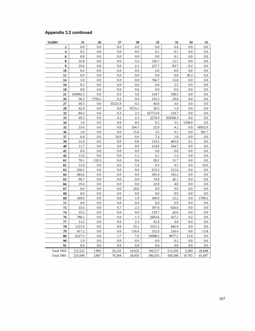
167
To2001 21 26 27 28 33 4
2 0. 0.0 0.0 0.0 0.0 0 0
Appendix 3.2 continued
32 3 35 0 0.0 0. 0.
4 9.2 0 0.0 0.0 0.1 0 0 .0 0.1 0. 0.6 0.8 0.0 0.0 0.1 0 0 0.0 0.0 0. 0.8 8 0.0 0.0 15 7 0 0 55. 5.5 6.7 12. 0. 0.9 6 0.0 0.6 2.1 7 2 0 35. 127.7 83. 0. 0.
10 0.0 0.0 0.0 0.0 0.0 0 0 0.0 0. 0.11 0.0 0.0 0. 0.0 0. .3 0 0 0.0 0 30 0.14 5.9 0.0 0.0 0.0 78 8 0 0 4.7 15. 0. 0.16 8.3 0.0 0.0 0.0 2.5 0 0 6.0 0. 0.18 0.0 0.0 0. 0. 0.0 0 0 0 0 0.0 0. 0.21 3 0.0 0 5. 13 8.5 0 0 104992. .5 0 4.7 16 0. 0.26 3 1793.2 0 0.0 13 0 0 0 56. .2 5.5 20. 0. 0.27 5 0.0 1. 0. 6 4.0 0 0 49. 3513 9 2 0.8 0. 0.28 4 0.0 0.0 9723. 2 1.4 0 0 42. 1 0.5 0. 0.32 2 0.0 0.3 2. 16771 9.7 0 0 84. 3 3.0 51 0. 0.33 3 0.0 0. 2. 227 3 0 0 49. 2 3 8.9 203568. 0. 0.34 1.0 0.0 0.0 0. 3.5 .0 0 0 0.5 5338 0.35 6 0.0 0.0 104.7 2 4.2 0 1 6 33. 5.9 0. 8932.36 1.8 0.0 0.0 15. 0.1 0 .7 8 3.5 0. 18137 0.4 0.0 16.0 0. 1.8 0 0 0 7.4 0. 0.39 0 0.0 0.0 0.0 11 3.9 1 0 21. 0.5 40 0. 0.40 7 0.0 0. 0.0 11 4.7 0 0 11. 0 4.6 16 0. 0.41 0.0 0.0 0.0 0.0 0 0 0.0 0.0 0. 0.42 6 0.0 0. 1.2 1.4 0 0 11. 0 6.1 0. 0.61 1 110.3 0.0 5 7 0 0 70. 0.6 8.1 31. 0. 0.62 0 0.0 0.0 4.3 0 .0 12. 5.4 9.3 0. 1063 6.5 0.0 0.0 0. 62 5.6 0 0 63 0 3.3 21 0. 0.64 3.6 0.0 0.0 0.0 29 5.2 0 0 49 5.4 16 0. 0.65 7 0.0 0.0 0.0 7 1 0 0 96. 4.8 42. 0. 0.66 4 0.0 0.0 0. 2 4.8 0 0 19. 0 3.9 0. 0.67 0.0 0.0 0.0 1 0.0 0 0 0.6 0.0 0. 0.68 0.0 0.0 0.0 0. 0.0 0 0 0 0.0 0. 0.69 9.0 0.0 0.0 10 2 0 .3 16 1.9 0.0 12. 0. 170871 0.0 0.0 0. 0.0 0 0 0 0.0 0.0 0. 0.73 6 0.0 0. 18 6.6 0 0 33. 7 2.3 7.6 62 0. 0.74 5 0.0 0.0 11 6 0 0 55. 0.0 9.7 42. 0. 0.76 6.1 0.0 0.0 266 7.1 2 0 78 1.3 3.6 42 0. 0.77 5 0.0 0.0 4 4.8 0 0 13. 2.3 1.8 0. 0.78 1.8 0.0 0.0 15. 332 5.9 0 0 112 1 1.5 44 0. 0.79 7.2 0.0 0.0 116.6 31 6.4 0 .8 41 3.3 21 0. 1580 7.3 0. 1 106 77.2 .9 0 612 0 .7 7.0 98.2 80 13 0.90 1.9 0. 0.1 0 0 0 0.0 0.0 0.0 0. 0.91 0.0 0.0 0.0 0.0 0.0 0.0 0.0 0.0
Total 1992 115,525 1,903 35,152 10,025 190,217 215,293 5,383 20,848 Total 2001 231,049 3,807 70,304 20,050 380,435 430,586 10,765 41,697
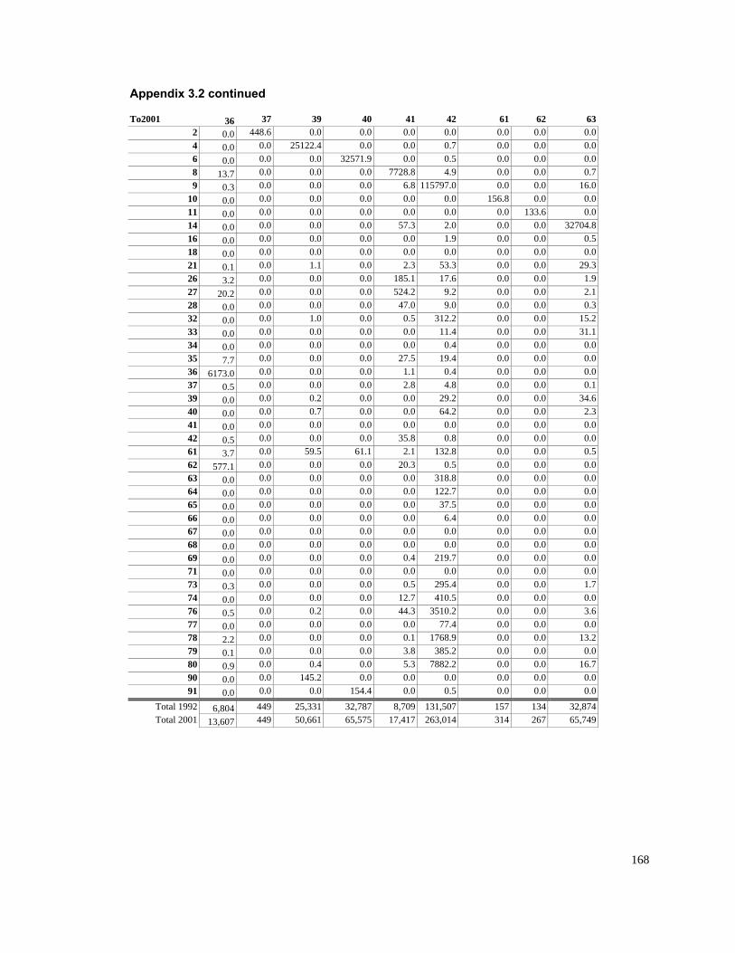
168
T 36 37 39 40 41 6 62
0. 448.6 0.0 0.0 0 0 0
Appendix 3.2 continued
o2001 42 1 632 0 0. 0.0 .0 .0 0.04 0. 0.0 25122.4 0.0 0 0 00 0. 0.7 .0 .0 0.06 0. 0.0 0.0 71.9 .0 0 0.0 325 0 0.5 .0 0 0.08 13 0.0 0.0 0.0 .8 0.7 7728 4.9 0.0 .0 0.79 0 0.0 0.0 0.0 8 115 0. 1.3 6. 797.0 0.0 0 6.0
10 0. 0.0 0.0 0.0 0 156 00 0. 0.0 .8 .0 0.011 0. 0.0 0.0 0.0 0 0 130 0. 0.0 .0 3.6 0.014 0. 0.0 0.0 0.0 .3 0 32700 57 2.0 0.0 .0 4.816 0. 0.0 0.0 0.0 0 00 0. 1.9 0.0 .0 0.518 0. 0.0 0.0 0.0 0 0 00 0. 0.0 .0 .0 0.021 0.0 1.1 0.0 3 0. 20.1 2. 53.3 0.0 0 9.326 0. 0.0 0.0 .1 0.3.2 0 185 17.6 0.0 0 1.927 20 0. 0.0 .2 0.2 0 0.0 524 9.2 0.0 .0 2.128 0 0.0 0. 0.0 .0 0 0.0 0 47 9.0 .0 .0 0.332 0 0.0 1.0 0.0 5 0. 1.0 0. 312.2 0.0 0 5.233 0 0.0 0.0 0.0 0 0. 3.0 0. 11.4 0.0 0 1.134 0. 0.0 0.0 0.0 00 0. 0.4 0.0 0.0 0.035 7 0.0 0.0 0.0 .5 1 0.7 27 9.4 .0 0.0 0.036 6173. 0.0 0.0 0.0 1 0 00 1. 0.4 .0 .0 0.037 0. 0.0 0.0 0.0 8 0 05 2. 4.8 .0 .0 0.139 0. 0.0 0.2 0.0 0 2 0 0. 30 0. 9.2 .0 0 4.640 0 0.0 0.7 0.0 0 0..0 0. 64.2 0.0 0 2.341 0 0.0 0.0 0.0 0 0.0 0. 0.0 0.0 .0 0.042 0. 0.0 0.0 0.0 .8 0 05 35 0.8 .0 .0 0.061 3 0.0 59.5 61.1 .1 13 0 0..7 2 2.8 .0 0 0.562 577 0. 0 0.0 .3 0.1 0 0. 20 0.5 0.0 .0 0.063 0.0 0.0 0.0 0 31 0 0.0.0 0. 8.8 .0 0 0.064 0.0 0.0 0.0 0 0.0.0 0. 122.7 0.0 0 0.065 0.0 0.0 0.0 0 0.0.0 0. 37.5 0.0 0 0.066 0 0.0 0.0 0.0 0 0.0 0. 6.4 0.0 .0 0.067 0 0.0 0.0 0.0 0 0 0.0 0. 0.0 .0 .0 0.068 0. 0.0 0.0 0.0 0 0 00 0. 0.0 .0 .0 0.069 0. 0.0 0.0 0.0 4 21 0 0.0 0. 9.7 .0 0 0.071 0.0 0.0 0.0 0 00.0 0. 0.0 0.0 .0 0.073 0. 0.0 0.0 0.0 5 29 0 0.3 0. 5.4 .0 0 1.774 0 0.0 0.0 0.0 .7 0..0 12 410.5 0.0 0 0.076 0 0.0 0.2 0.0 .3 3 0..5 44 510.2 0.0 0 3.677 0.0 0.0 0.0 0 0.0.0 0. 77.4 0.0 0 0.078 2 0.0 0.0 0.0 1 17 0 0. 1.2 0. 68.9 .0 0 3.279 0.0 0.0 0.0 8 0.0.1 3. 385.2 0.0 0 0.080 0.0 0.4 0.0 3 7 0.0.9 5. 882.2 0.0 0 16.790 0.0 145.2 0.0 00.0 0. 0.0 0.0 0.0 0.091 0. 0.0 0.0 54.4 .0 0 0.0 1 0 0.5 .0 0 0.0
Total 1992 6,80 449 25,331 ,787 09 131,5 1 134 32,84 32 8,7 07 57 74Total 2001 1 449 50,661 ,575 173,607 65 17,4 263,014 314 267 65,749
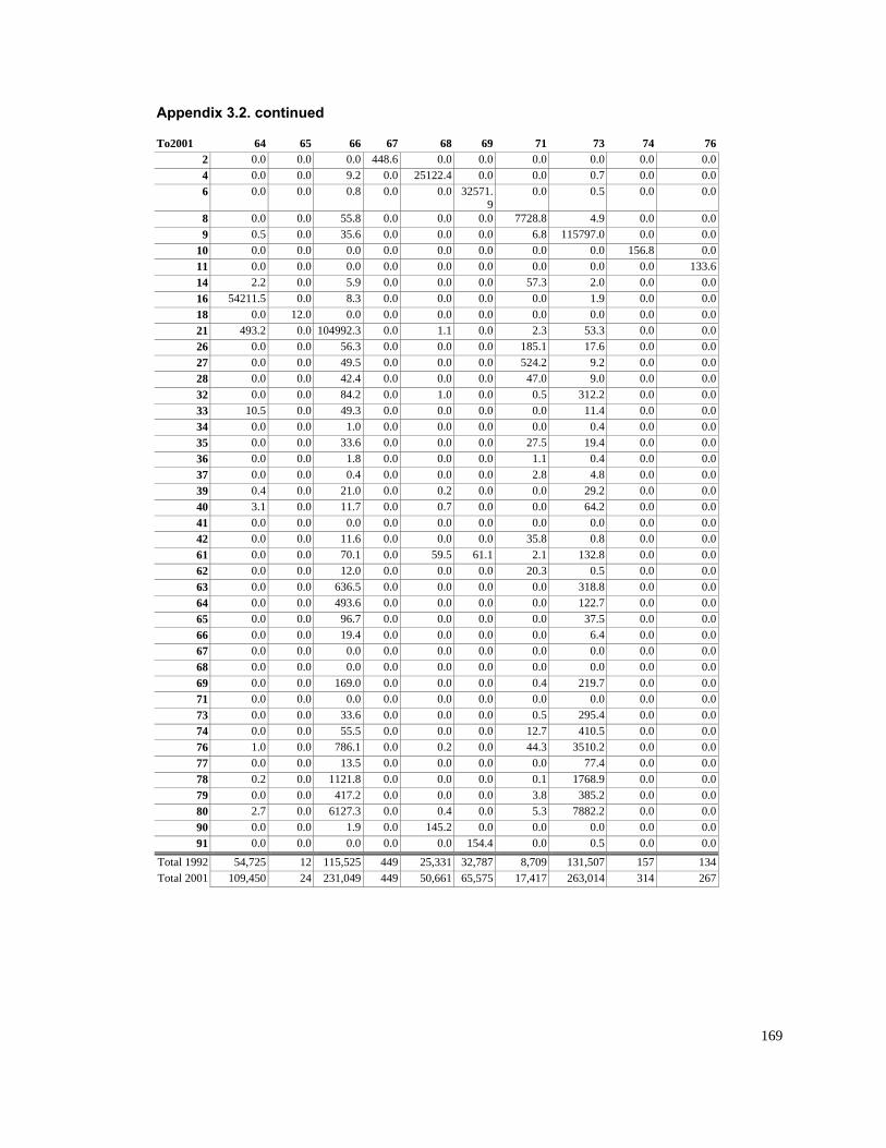
169
64 65 66 6 7
2 0.0 0.0 6 0. 0.
Appendix 3.2. continued
To2001 67 68 9 71 3 74 760.0 448. 0.0 0 0.0 0 0.0 0.0
4 0.0 0.0 0 251 0 0 9.2 0. 22.4 .0 0.0 .7 0.0 0.06 0.0 0.0 0.8 0 3257 0 0. 0.0 1.
90.0 .5 0.0 0.0
8 0. 0.0 55.8 0 40 0. 0.0 0.0 7728.8 .9 0.0 0.09 0.5 0.0 35.6 0 0 1157 0. 0.0 .0 6.8 97.0 0.0 0.0
10 0.0 0.0 0.0 0 0 0. 0.0 .0 0.0 0.0 156.8 0.011 0.0 0.0 0.0 0 0 0. 0.0 0.0 0.0 .0 0.0 133.614 2.2 0.0 5.9 0 5 2 0. 0.0 0.0 7.3 .0 0.0 0.016 11.5 0.0 8.3 0 0 1542 0. 0.0 .0 0.0 .9 0.0 0.018 0.0 12.0 0.0 0 0 00. 0.0 .0 0.0 .0 0.0 0.021 2 0.0 992.3 0 53.493. 104 0. 1.1 0.0 2.3 3 0.0 0.026 0. 0.0 56.3 0 18 17.0 0. 0.0 0.0 5.1 6 0.0 0.027 0. 0.0 49.5 0 52 90 0. 0.0 0.0 4.2 .2 0.0 0.028 0.0 0.0 42.4 0 0 9 0. 0.0 .0 47.0 .0 0.0 0.032 0.0 0.0 84.2 0 0 312. 0. 1.0 .0 0.5 2 0.0 0.033 10.5 0.0 49.3 0 0 11. 0. 0.0 .0 0.0 4 0.0 0.034 0.0 0.0 1.0 0 0 0. 0.0 0.0 0.0 .4 0.0 0.035 0.0 33.6 0 0 2 19.0.0 0. 0.0 .0 7.5 4 0.0 0.036 0.0 1.8 0 0 00.0 0. 0.0 .0 1.1 .4 0.0 0.037 0.0 0.0 0.4 0 0 4 0. 0.0 .0 2.8 .8 0.0 0.039 0.4 0.0 21.0 0 0 29. 0. 0.2 .0 0.0 2 0.0 0.040 3.1 0.0 11.7 0 0 64. 0. 0.7 .0 0.0 2 0.0 0.041 0.0 0.0 0.0 0 0 0. 0.0 0.0 0.0 .0 0.0 0.042 0.0 0.0 11.6 0 0 0. 0.0 0.0 35.8 .8 0.0 0.061 0.0 70.1 0 6 132.0.0 0. 59.5 1.1 2.1 8 0.0 0.062 0. 0.0 12.0 0 00 0. 0.0 0.0 20.3 .5 0.0 0.063 0.0 0.0 636.5 0 0 318. 0. 0.0 .0 0.0 8 0.0 0.064 0.0 0.0 493.6 0 0 122. 0. 0.0 .0 0.0 7 0.0 0.065 0.0 0.0 96.7 0 0 37. 0. 0.0 .0 0.0 5 0.0 0.066 0.0 0.0 19.4 0 0 6 0. 0.0 .0 0.0 .4 0.0 0.067 0.0 0.0 0.0 0 0 0 0. 0.0 .0 0.0 .0 0.0 0.068 0.0 0.0 0.0 0 0 0 0. 0.0 .0 0.0 .0 0.0 0.069 0.0 0.0 169.0 0 0 219. 0. 0.0 .0 0.4 7 0.0 0.071 0.0 0.0 0.0 0 0 0 0. 0.0 .0 0.0 .0 0.0 0.073 0.0 0.0 33.6 0 295. 0. 0.0 0.0 0.5 4 0.0 0.074 0.0 0.0 55.5 0 410. 0. 0.0 0.0 12.7 5 0.0 0.076 1.0 0.0 786.1 0 0 3510. 0. 0.2 .0 44.3 2 0.0 0.077 0.0 0.0 13.5 0 0 77. 0. 0.0 .0 0.0 4 0.0 0.078 0.2 0.0 121.8 0 0 1768. 1 0. 0.0 .0 0.1 9 0.0 0.079 0.0 0.0 417.2 0 0 385. 0. 0.0 .0 3.8 2 0.0 0.080 2.7 0.0 127.3 0 0 7882. 6 0. 0.4 .0 5.3 2 0.0 0.090 0.0 0.0 1.9 0 0 0 0. 145.2 .0 0.0 .0 0.0 0.091 0. 0. 0 0 1 00 0 .0 0. 0.0 54.4 0.0 .5 0.0 0.0
Total 1 5,52 9 3 131,51992 54,725 2 11 5 44 25,331 2,787 8,709 07 157 134Total 2001 24 04 65, 263,01 314 109,450 231, 9 449 50,661 575 17,417 4 267
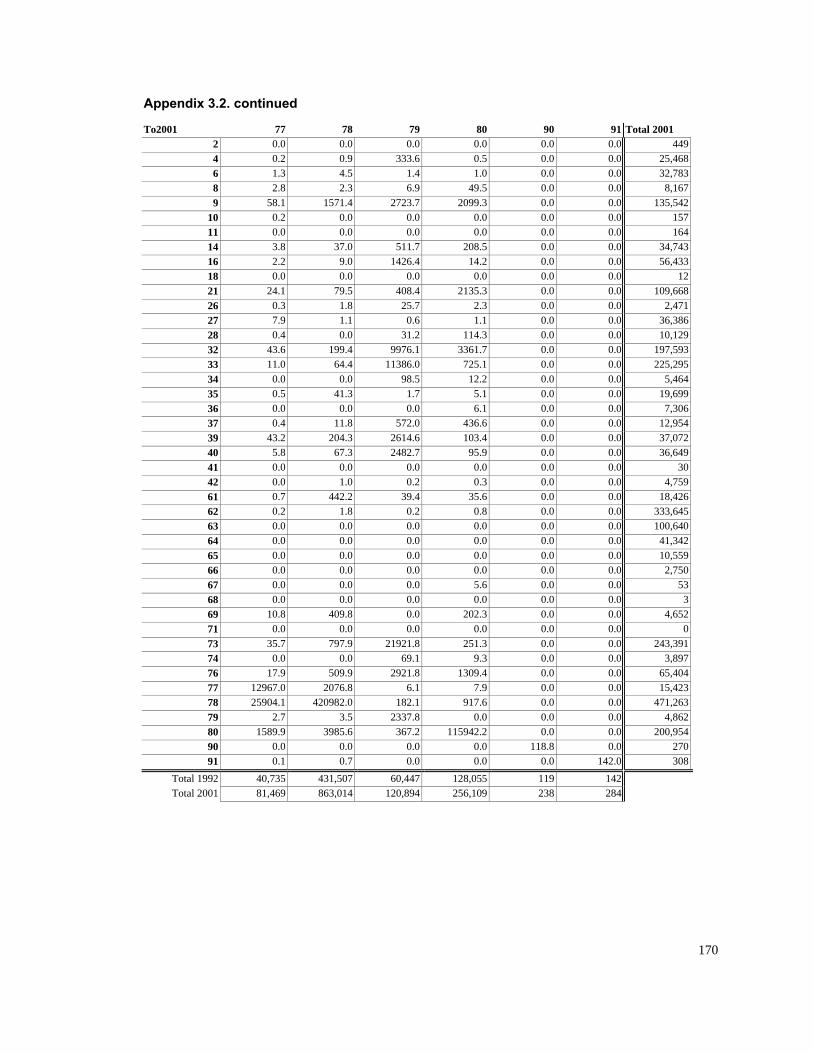
170
78 80 91 Tota 01
Appendix 3.2. continued To2001 77 79 90 l 20
2 0.0 0.0 4490.0 0.0 0.0 0.04 0. 0.5 0.0 4680.2 9 333.6 0.0 25,6 4. 1.0 0.0 7831.3 5 1.4 0.0 32,8 2.8 2.3 6.9 49.5 0.0 0.0 8,1679 5 71. 27 20 0.0 5,5428.1 15 4 23.7 99.3 0.0 13
10 0. 0.0 0.0 1570.2 0 0.0 0.011 0. 0.0 0.0 1640.0 0 0.0 0.014 37. 5 208.5 0.0 7433.8 0 11.7 0.0 34,16 9. 14 14. 0.0 4332.2 0 26.4 2 0.0 56,18 0.0 0. 0.0 0.0 120 0.0 0.021 79. 4 2135.3 0.0 9,66824.1 5 08.4 0.0 1026 1. 2.3 0.0 2,4710.3 8 25.7 0.027 1. 0.0 3867.9 1 0.6 1.1 0.0 36,28 0. 11 0.0 1290.4 0 31.2 4.3 0.0 10,32 4 99. 99 3361. 0.0 7,5933.6 1 4 76.1 7 0.0 1933 1 64. 113 725.1 0.0 5,2951.0 4 86.0 0.0 2234 0. 12.2 0.0 5,4640.0 0 98.5 0.035 41. 5.1 0.0 6990.5 3 1.7 0.0 19,36 0. 6. 0.0 7,3060.0 0 0.0 1 0.037 11. 5 436.6 0.0 9540.4 8 72.0 0.0 12,39 4 04. 26 103.4 0.0 0723.2 2 3 14.6 0.0 37,40 67. 24 95.9 0.0 6495.8 3 82.7 0.0 36,41 0. 0.0 0.0 300.0 0 0.0 0.042 1. 0.3 0.0 4,7590.0 0 0.2 0.061 42. 35. 0.0 4260.7 4 2 39.4 6 0.0 18,62 1. 0.8 0.0 3,6450.2 8 0.2 0.0 3363 0. 0. 0.0 0,6400.0 0 0.0 0 0.0 1064 0. 0.0 0.0 3420.0 0 0.0 0.0 41,65 0. 0.0 0.0 5590.0 0 0.0 0.0 10,66 0. 0.0 0.0 2,7500.0 0 0.0 0.067 0. 5.6 0.0 530.0 0 0.0 0.068 0. 0.0 0.0 30.0 0 0.0 0.069 1 09. 202.3 0.0 4,6520.8 4 8 0.0 0.071 0. 0.0 0.0 00.0 0 0.0 0.073 3 97. 219 251.3 0.0 3,3915.7 7 9 21.8 0.0 2474 0. 9.3 0.0 3,8970.0 0 69.1 0.076 1 09. 29 1309. 0.0 4047.9 5 9 21.8 4 0.0 65,77 1296 76. 7. 0.0 15,4237.0 20 8 6.1 9 0.078 2590 82. 1 917.6 0.0 1,2634.1 4209 0 82.1 0.0 4779 3. 23 0.0 0.0 4,8622.7 5 37.8 0.080 158 85. 3 5942.2 0.0 0,9549.9 39 6 67.2 11 0.0 2090 0. 0.0 0.0 2700.0 0 0.0 118.891 0. 0.0 2.0 3080.1 7 0.0 0.0 14
T 1992 40, ,50 60 055 142 otal 735 431 7 ,447 128, 119Total 200 81,4 ,01 1 284 1 69 863 4 120,894 256, 09 238
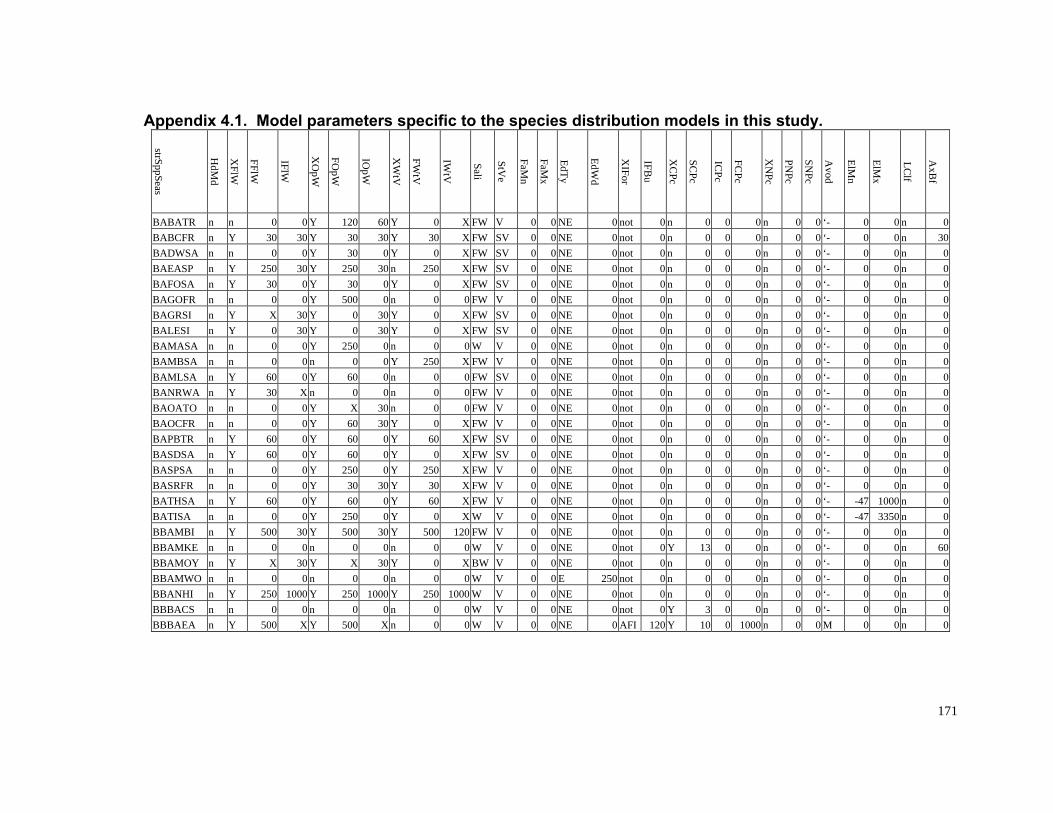
171
Appendix 4.1. Model parameters specific to the species distribution models in this study.
strSppSeas
HdM
d
XFlW
FF IFlW
XO
pW
FOpW
IOpW
XW
tV
FWtV
IWtV
Sali
StVe
FaMn
FaMx
EdTy
EdWd
XIFor
IFBu
XC
Pc
SCPc
ICPc
FCPc
XN
Pc
PNPc
SNPc
Avod
ElMn
ElMx
LClf f
lW
AxB
BABATR n n 0 0 Y 120 60 Y 0 X FW V 0 0 NE 0 not 0 n 0 0 0 n 0 0 ‘- 0 0 n 0BABCFR n Y 30 30 Y 30 30 Y 30 X FW SV 0 0 NE 0 not 0 n 0 0 0 n 0 0 ‘- 0 0 n 30BADWSA n n 0 0 Y 30 0 Y 0 X FW SV 0 0 NE 0 not 0 n 0 0 0 n 0 0 ‘- 0 0 n 0BAEASP n 30 30 n 250 X FW SV 0 0 NE 0 not 0 n 0 0 0 n 0 0 ‘- 0 0 n Y 250 Y 250 0BAFOSA n Y 30 0 Y 30 0 Y 0 X FW SV 0 0 NE 0 not 0 n 0 0 0 n 0 0 ‘- 0 0 n 0BAGOFR n n 0 0 Y 500 0 n 0 0 FW V 0 0 NE 0 not 0 n 0 0 0 n 0 0 ‘- 0 0 n 0BAGRSI n Y X 30 Y 0 30 Y 0 X FW SV 0 0 NE 0 not 0 n 0 0 0 n 0 0 ‘- 0 0 n 0BALESI n 30 Y 0 X FW SV 0 0 NE 0 not 0 n 0 0 0 n 0 0 ‘- 0 0 n 0Y 0 30 Y 0BAMASA n n 00 0 Y 250 0 n 0 0 W V 0 0 NE 0 not 0 n 0 0 0 n 0 0 ‘- 0 0 n BAMBSA n 0n 0 0 n 0 0 Y 250 X FW V 0 0 NE 0 not 0 n 0 0 0 n 0 0 ‘- 0 0 n BAMLSA n Y 60 0 Y 60 0 n 0 0 FW SV 0 0 NE 0 not 0 n 0 0 0 n 0 0 ‘- 0 0 n 0BANRWA n Y 0 X n 0 0 0 FW V 0 0 NE 0 not 0 n 0 0 0 n 0 0 ‘- 0 0 n 03 n 0BAOATO n n 0 0 0 FW V 0 E 0 0 ‘- 0 00 Y X 30 n 0 N 0 not n 0 0 0 n 0 0 nBAOCFR n n 00 0 Y 60 30 Y 0 X FW V 0 0 NE 0 not 0 n 0 0 0 n 0 0 ‘- 0 0 n BAPBTR n Y 60 0 Y 60 0 Y 60 X FW SV 0 0 NE 0 not 0 n 0 0 0 n 0 0 ‘- 0 0 n 0BASDSA n Y 60 Y 60 0 Y 0 X FW SV 0 0 NE 0 not 0 n 0 0 0 n 0 0 ‘- 0 0 n 00 BASPSA n n 0 Y 2 X FW V 0 0 NE 0 n 0 ‘- 0 0 n 00 Y 250 0 50 0 not 0 0 0 n 0BASRFR n n 00 0 Y 30 30 Y 30 X FW V 0 0 NE 0 not 0 n 0 0 0 n 0 0 ‘- 0 0 n BATHSA n Y 60 0 Y 60 0 Y 60 X FW V 0 0 NE 0 not 0 n 0 0 0 n 0 0 ‘- -47 1000 n 0BATISA n n 0 0 Y 250 0 Y 0 X W V 0 0 NE 0 not 0 n 0 0 0 n 0 0 ‘- -47 3350 n 0BBAMBI n Y 500 30 Y 500 30 Y 500 120 FW V 0 0 NE 0 not 0 n 0 0 0 n 0 0 ‘- 0 0 n 0BBAMKE n n 600 0 n 0 0 n 0 0 W V 0 0 NE 0 not 0 Y 13 0 0 n 0 0 ‘- 0 0 n BBAMOY n 0Y X 30 Y X 30 Y 0 X BW V 0 0 NE 0 not 0 n 0 0 0 n 0 0 ‘- 0 0 n BBAMWO n n 0 0 n 0 0 n 0 0 W V 0 0 E 250 not 0 n 0 0 0 n 0 0 ‘- 0 0 n 0BBANHI n Y 250 1000 Y 250 1000 Y 250 1000 W V 0 0 NE 0 not 0 n 0 0 0 n 0 0 ‘- 0 0 n 0BBBACS n n 0 n 0 0 n 0 0 W V 0 0 NE 0 not 0 Y 3 0 0 n 0 0 ‘- 0 0 n 00 BBBAEA n Y 0500 X Y 500 X n 0 0 W V 0 0 NE 0 AFI 120 Y 10 0 1000 n 0 0 M 0 0 n
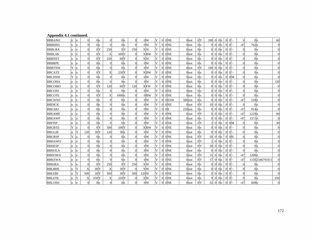
172
0 n 60
Appendix 4.1 continued. BBBANO n n 0 0 n 0 0 n 0 0 W V 0 0 NE 0 not 0 Y 100 0 0 n 0 0 ‘- 0BBBHNU n n 0 0 n 0 0 n 0 0 W V 0 0 NE 0 not 0 n 0 0 0 n 0 0 ‘- -47 762 n 0BBBLRA 0 0 X E not n n 0 Y 250 0 Y 25 W V 0 0 N 0 0 n 0 0 0 n 0 0 ‘- 0 0 n 0BBBLSK 0 0 E n n n 0 Y X 500 Y X BW V 0 0 N 0 ot 0 n 0 0 0 n 0 0 ‘- 0 0 n 0BBBNST n n 0 Y 250 60 Y 0 X W V 0 0 NE 0 not 0 n 0 0 0 n 0 0 ‘- 0 0 n 00 BBBRPE n n 0 0 n 0 0 n 0 0 W V 0 0 NE 0 not 0 n 0 0 0 n 0 0 ‘- 0 0 n 0BBBTNW Y 0 n 0 0 0 0 0 ‘- 0n 0 n 0 W V 0 0 NE 0 not 0 Y 100 0 n 0 0 0 n BBCATE n n 0 Y X 50 Y 0 0 0 0 ‘- 0 2 X BW V 0 0 NE 0 not 0 n 0 n 0 0 0 n 0BBCHSW Y 0 n 0 0 0 0 0 M 0n 0 n 0 0 W V 0 0 NE 0 not 0 n 0 n 0 0 0 n BBCOHA n 0 n 0 0 0 0 0 ‘- 120n 0 n 0 0 W V 0 0 NE 0 not 0 n 0 n 0 0 0 n BBCOMO n 0 Y 120 60 120 0 0 0 ‘- 0 n 0 Y X FW V 0 0 NE 0 not 0 n 0 n 0 0 0 n BBCONI n 0 n 0 0 0 0 0 ‘- 0n 0 n 0 0 W V 0 0 NE 0 not 0 n 0 n 0 0 0 n BBCOTE n 0 Y X 00 0 0 0 ‘- 0n 0 10 n 0 0 BW V 0 0 NE 0 not 0 n 0 n 0 0 0 n BBCWWI n 0 n 0 0 W 0 0 0 ‘- - 518 0n 0 n 0 0 W V 0 0 ES 500 not 0 n 0 n 0 47 n BBDICK n 0 n 0 0 0 0 0 0 ‘- 0n 0 n 0 W V 0 0 NE 0 not 0 Y 1 0 n 0 0 0 n BBEAKI n 0 n 0 0 0 0 0 ‘- - 914 0n 0 n 0 0 W V 0 0 E 250 not 0 n 0 n 0 47 n BBEAME n 0 n 0 0 0 6 0 0 ‘- - 1219 60n 0 n 0 W V 0 0 NE 0 not 0 Y 0 n 0 47 n BBEAWP n 0 n 0 0 0 0 0 ‘- - 1371 0n 0 n 0 0 W V 0 0 NE 0 not 0 n 0 n 0 47 n BBFISP n n 0 n 0 0 n 0 2 0 0 M 300 0 W V 0 0 NE 0 not 0 Y 0 n 0 0 0 n BBGBTE Y 0 Y 500 00 Y 0 0 0 0 ‘- 0n 0 5 X BW V 0 0 NE 0 not 0 n 0 n 0 0 0 n BBGLIB n 30 120 30 0 0 0 ‘- 0Y 120 Y n 0 0 W V 0 0 NE 0 not 0 n 0 n 0 0 0 n BBGRSP Y 0 n 0 0 0 0 0 0 H 0n 0 n 0 W V 0 0 NE 0 not 0 Y 5 0 n 0 0 0 n BBHAWO n 0 n 0 0 0 2 0 0 ‘- 0 n 0 n 0 W V 0 0 NE 0 not 0 Y 0 n 0 0 0 n BBHESP n 0 n 0 0 0 0 0 0 ‘- 0n 0 n 0 W V 0 0 NE 0 not 0 Y 3 0 n 0 0 0 n BBHOLA n 0 n 0 0 0 0 0 ‘- 0n 0 n 0 0 W V 0 0 NE 0 not 0 n 0 n 0 0 0 n BBHOWA n 0 n 0 0 0 0 5 0 0 ‘- - 12 0 n 0 n W V 0 0 NE 0 not 0 Y 1 0 n 0 47 00 n BBKEWA n 0 n 0 0 n 7 0 0 ‘- - 1150 3467 1 0 n 0 0 0 W V 0 0 NE 0 not 0 Y 1 0 n 0 47 2 9101BBKIRA n 0 Y 250 0 Y 250 0 0 0 ‘- n 0 X W V 0 0 NE 0 not 0 n 0 n 0 0 0 n 0BBLBHE n Y 30 X 30 Y 0 0 0 0 ‘- 0X Y X W V 0 0 NE 0 not 0 n 0 n 0 0 0 n BBLEBI n Y 30 500 30 Y 500 E 0 0 0 ‘- 0500 Y 120 W V 0 0 N 0 not 0 n 0 n 0 0 0 n BBLETE n 0 Y 50 0 0 0 ‘- 250Y X 25 X 2 Y 0 X W V 0 0 NE 0 not 0 n 0 n 0 0 0 n BBLOSH n 0 n 0 0 0 0 2 0 0 ‘- - 600 0n 0 n W V 0 0 NE 0 not 0 Y 5 0 n 0 47 n
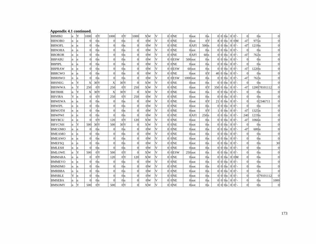
173
Appendix 4.1 continued. 0 Y 1000 0 Y 1000 X W V 0 0 NE 0 not 0 n 0 0 0 n 0 0 ‘- 0 0 n 0
BBMIKI n Y 1000BBNOBO n n 0 0 n 0 V E Y n - 970 n 0 0 W 0 0 N 0 not 0 8 0 0 0 0 M 47 5 n 0BBNOFL n n 0 0 n 0 n V E 0 n 1 00 0 0 W 0 0 N 0 AFI 50 n 0 0 0 0 0 ‘- -47 219 n BBNOHA 0 V E 0 n n 0n n 0 0 n 0 n 0 0 W 0 0 N 0 not 0 0 0 0 0 ‘- 0 0 n BBOROR 0 V E 0 n n - 76 0n n 0 0 n 0 n 0 0 W 0 0 N 0 AFI 6 0 0 0 0 0 ‘- 47 2 n BBPABU 0 V W 0 n n 0n n 0 0 n 0 n 0 0 W 0 0 ES 500 not 0 0 0 0 0 ‘- 0 0 n BBPIPL n n 0 0 n 0 n E 0 n n 00 0 0 W V 0 0 N 0 not 0 0 0 0 0 ‘- 0 0 n BBPRAW n n 0 0 n 0 V W n n - 122 00 n 0 0 W 0 0 ES 60 not 0 0 0 0 0 0 ‘- 47 0 n BBRCWO 0 E 0 Y n 0n n 0 0 n 0 n 0 0 W V 0 0 N 0 not 40 0 0 0 0 ‘- 0 0 n BBRHWO 0 W 0 n n - 76 0n n 0 0 n 0 n 0 0 W V 0 0 ES 1000 not 0 0 0 0 0 ‘- 47 2 n BBSNEG X 3 V E 0 n nn Y X 30 Y 0 Y 0 X W 0 0 N 0 not 0 0 0 0 0 ‘- 0 0 n 0BBSWWA 250 0 0 E 0 Y n - 120 01112n Y Y 25 0 Y 250 X W V 0 0 N 0 not 350 0 0 0 0 ‘- 47 0 781 0BBTRHE X 3 V E 0 n n 0 n Y X 30 Y 0 Y 0 X W 0 0 N 0 not 0 0 0 0 0 ‘- 0 0 n BBVIRA Y n 0 0 Y 250 2 V E 0 n n 00 Y 50 0 W 0 0 N 0 not 0 0 0 0 0 ‘- 0 0 n BBWEWA 0 0 Y n 6711 0n n 0 0 n 0 n 0 0 W V 0 0 NE 0 not 21 0 0 0 0 ‘- 0 0 234BBWIPL 0 n V n n 0 n n 0 0 n 0 0 0 W 0 0 NE 0 not 0 0 0 0 0 0 ‘- 0 0 n BBWOTH 0 NE 0 Y n 1 0n n 0 0 n 0 n 0 0 W V 0 0 0 not 1 0 0 0 0 ‘- -47 325 n BBWPWI 0 V E n n n n 0 0 n 0 n 0 0 W 0 0 N 0 AFI 250 0 0 0 0 0 ‘- 240 1219 n 0BBYBCU 1 V E 0 n n 0n n 0 0 Y 120 0 Y 20 X W 0 0 N 0 not 0 0 0 0 0 ‘- -47 1066 n BBYCNH 5 30 Y V E n nn Y 00 30 Y 500 0 X W 0 0 N 0 not 0 0 0 0 0 0 ‘- 0 0 n 0BMCOMO 0 0 E 0 n n - 60 0n n 0 n 0 n 0 0 W V 0 0 N 0 not 0 0 0 0 0 ‘- 47 0 n BMEAMO 0 E 0 n n 0n n 0 0 n 0 n 0 0 W V 0 0 N 0 not 0 0 0 0 0 ‘- 0 0 n BMEAWO 0 E n n 0n n 0 0 n 0 n 0 0 W V 0 0 N 0 not 0 0 0 0 0 0 ‘- 0 0 n BMEFSQ 0 V E n n 30n n 0 0 n 0 n 0 0 W 0 0 N 0 not 0 0 0 0 0 0 ‘- 0 0 n BMLESH n 0 V E n n 0n 0 0 n 0 n 0 0 W 0 0 N 0 not 0 0 0 0 0 0 ‘- 0 0 n BMLOWE 500 W 0 n n 0n Y 0 Y 500 0 Y 0 X W V 0 0 ES 250 not 0 0 0 0 0 ‘- 0 0 n BMMARA 1 E n n 0n n 0 0 Y 120 0 Y 20 X W V 0 0 N 0 not 0 0 0 0 0 0 M 0 0 n BMMEVO 0 E n n 0n n 0 0 n 0 n 0 0 W V 0 0 N 0 not 0 0 0 0 0 0 ‘- 0 0 n BMMJMO 0 0 E 0 n n 0n n 0 n 0 n 0 0 W V 0 0 N 0 not 0 0 0 0 0 ‘- 0 0 n BMRBBA 0 V E 0 n n 0n n 0 0 n 0 n 0 0 W 0 0 N 0 not 0 0 0 0 0 ‘- 0 0 n BMSBLE 0 V E 0 n n 01112 0 Y n 0 0 n 0 n 0 0 W 0 0 N 0 not 0 0 0 0 0 ‘- 0 0 791BMSEBA 0 V E 0 n n 10n n 0 0 n 0 n 0 0 W 0 0 N 0 not 0 0 0 0 0 ‘- 0 0 n 00BMSOMY 500 E n nn Y 0 Y 500 0 Y 0 X W V 0 0 N 0 not 0 0 0 0 0 0 ‘- 0 0 n 0
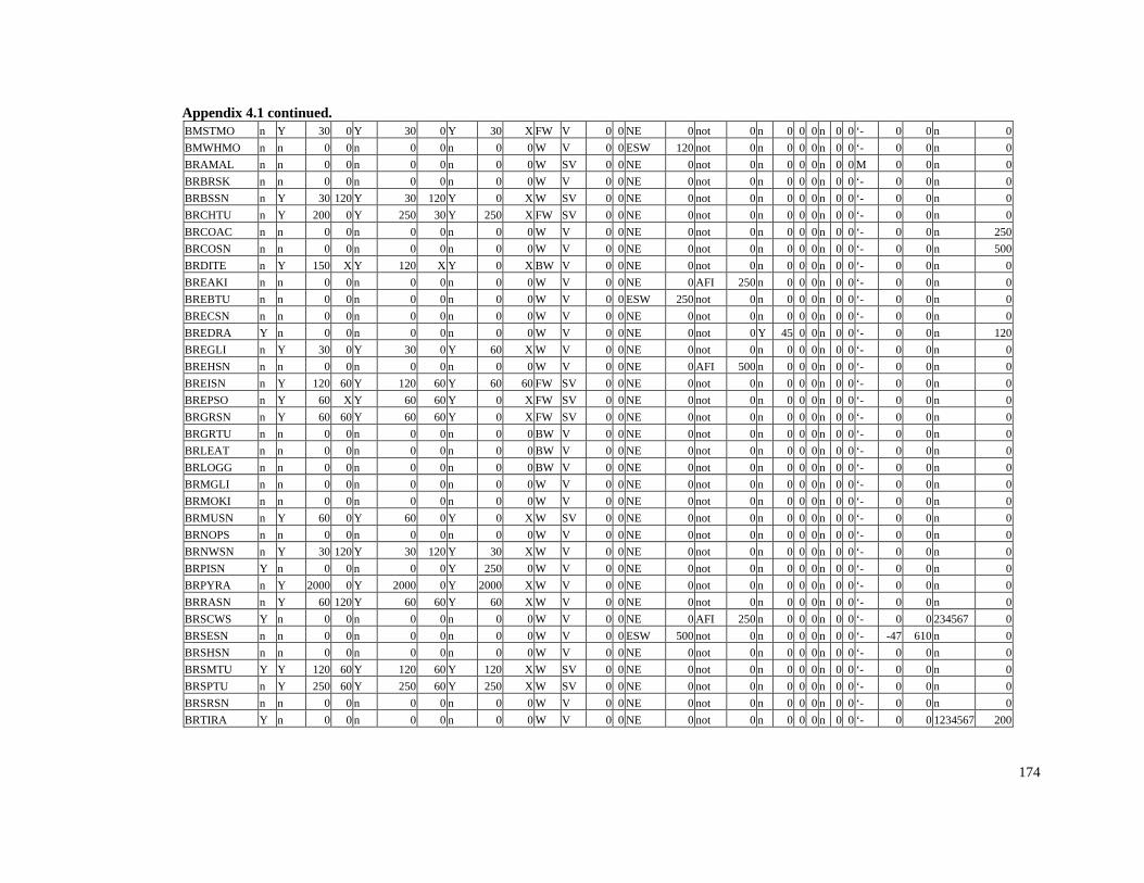
174
Appendix 4.1 continued.
O BMSTM n Y 30 0 Y 30 0 Y 30 X FW V 0 0 NE 0 not 0 n 0 0 0 n 0 0 ‘- 0 0 n 0BMWHMO 1 n n 0 0 n 0 0 n 0 0 W V 0 0 ESW 20 not 0 n 0 0 0 n 0 0 ‘- 0 0 n 0BRAMAL n n 0 0 n 0 0 n 0 0 W SV 0 0 NE 0 not 0 n 0 0 0 n 0 0 M 0 0 n 0BRBRSK n n 0 0 n 0 0 n 0 0 W V 0 0 NE 0 not 0 n 0 0 0 n 0 0 ‘- 0 0 n 0BRBSSN n Y 30 120 Y 30 1 20 Y 0 X W SV 0 0 NE 0 not 0 n 0 0 0 n 0 0 ‘- 0 0 n 0BRCHTU n Y 2 2 2 00 0 Y 50 30 Y 50 X FW SV 0 0 NE 0 not 0 n 0 0 0 n 0 0 ‘- 0 0 n 0BRCOAC 2n n 0 0 n 0 0 n 0 0 W V 0 0 NE 0 not 0 n 0 0 0 n 0 0 ‘- 0 0 n 50BRCOSN n n 0 0 n 0 0 n 0 0 W V 0 0 NE 0 not 0 n 50 0 0 n 0 0 ‘- 0 0 n 00BRDITE n Y 1 1 50 X Y 20 X Y 0 X BW V 0 0 NE 0 not 0 n 0 0 0 n 0 0 ‘- 0 0 n 0BREAKI n n 0 0 n 0 0 n 0 0 W V 0 0 NE 0 AFI 250 n 0 0 0 n 0 0 ‘- 0 0 n 0BREBTU n n 0 0 n 0 0 n 0 0 W V 0 0 ESW 250 not 0 n 0 0 0 n 0 0 ‘- 0 0 n 0BRECSN n n 0 0 n 0 0 n 0 0 W V 0 0 NE 0 not 0 n 0 0 0 n 0 0 ‘- 0 0 n 0BREDRA Y n 0 0 n 0 0 n 0 0 W V 0 0 NE 0 not 0 Y 145 0 0 n 0 0 ‘- 0 0 n 20BREGLI n Y 30 0 Y 30 0 Y 60 X W V 0 0 NE 0 not 0 n 0 0 0 n 0 0 ‘- 0 0 n 0BREHSN n n 0 0 n 0 0 n 0 0 W V 0 0 NE 0 AFI 500 n 0 0 0 n 0 0 ‘- 0 0 n 0BREISN n Y 1 1 20 60 Y 20 60 Y 60 60 FW SV 0 0 NE 0 not 0 n 0 0 0 n 0 0 ‘- 0 0 n 0BREPSO n Y 60 X Y 60 60 Y 0 X FW SV 0 0 NE 0 not 0 n 0 0 0 n 0 0 ‘- 0 0 n 0BRGRSN n Y 60 60 Y 60 60 Y 0 X FW SV 0 0 NE 0 not 0 n 0 0 0 n 0 0 ‘- 0 0 n 0BRGRTU n n 0 0 n 0 0 n 0 0 BW V 0 0 NE 0 not 0 n 0 0 0 n 0 0 ‘- 0 0 n 0BRLEAT n n 0 0 n 0 0 n 0 0 BW V 0 0 NE 0 not 0 n 0 0 0 n 0 0 ‘- 0 0 n 0BRLOGG n n 0 0 n 0 0 n 0 0 BW V 0 0 NE 0 not 0 n 0 0 0 n 0 0 ‘- 0 0 n 0BRMGLI n n 0 0 n 0 0 n 0 0 W V 0 0 NE 0 not 0 n 0 0 0 n 0 0 ‘- 0 0 n 0BRMOKI n n 0 0 n 0 0 n 0 0 W V 0 0 NE 0 not 0 n 0 0 0 n 0 0 ‘- 0 0 n 0BRMUSN n Y 60 0 Y 60 0 Y 0 X W SV 0 0 NE 0 not 0 n 0 0 0 n 0 0 ‘- 0 0 n 0BRNOPS n n 0 0 n 0 0 n 0 0 W V 0 0 NE 0 not 0 n 0 0 0 n 0 0 ‘- 0 0 n 0BRNWSN n Y 30 120 Y 30 1 20 Y 30 X W V 0 0 NE 0 not 0 n 0 0 0 n 0 0 ‘- 0 0 n 0BRPISN Y n 0 0 n 0 0 Y 250 0 W V 0 0 NE 0 not 0 n 0 0 0 n 0 0 ‘- 0 0 n 0BRPYRA n Y 20 2 2 00 0 Y 000 0 Y 000 X W V 0 0 NE 0 not 0 n 0 0 0 n 0 0 ‘- 0 0 n 0BRRASN n Y 60 120 Y 60 60 Y 60 X W V 0 0 NE 0 not 0 n 0 0 0 n 0 0 ‘- 0 0 n 0BRSCWS Y n 0 0 n 0 0 n 0 0 W V 0 0 NE 0 AFI 567 250 n 0 0 0 n 0 0 ‘- 0 0 234 0BRSESN n n 0 0 n 0 0 n 0 0 W V 0 0 ESW - 610500 not 0 n 0 0 0 n 0 0 ‘- 47 n 0BRSHSN n n 0 0 n 0 0 n 0 0 W V 0 0 NE 0 not 0 n 0 0 0 n 0 0 ‘- 0 0 n 0BRSMTU Y Y 120 60 Y 120 60 Y 1 20 X W SV 0 0 NE 0 not 0 n 0 0 0 n 0 0 ‘- 0 0 n 0BRSPTU n Y 250 Y Y 250 SV not 0 n 60 250 60 X W 0 0 NE 0 0 n 0 0 0 n 0 0 ‘- 0 0BRSRSN n n 0 0 n 0 0 n 0 0 W V 0 0 NE 0 not 0 n 0 0 0 n 0 0 ‘- 0 0 n 0BRTIRA Y n 0 0 n 0 0 n 0 0 W V 0 0 NE 0 not 0 n 0 0 0 n 0 0 ‘- 0 0 1234567 200
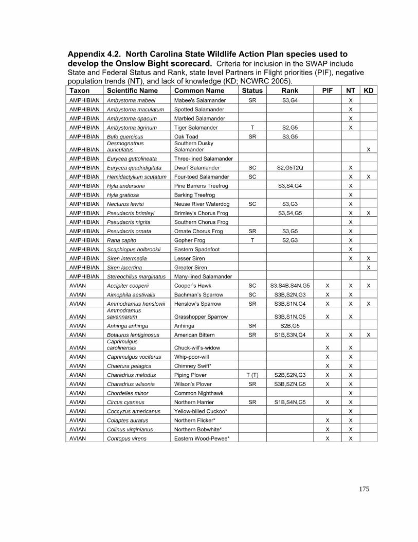
175
Appendix 4.2. North Carolina State Wildlife Action Plan species used to e
State and Federal Status and Rank, state level Partners in Flight priorities (PIF), negative population trends (NT), and lack of knowledge (KD; NCWRC 2005). Taxon Scientific Name Common Name Status Rank PIF NT KD
develop the Onslow Bight scorecard. Criteria for inclusion in the SWAP includ
AMPHIBIAN Ambystoma mabeei Mabee's Salamander SR S3,G4 X AMPHIBIAN Ambystoma maculatum Spotted Salamander X AMPHIBIAN Ambystoma opacum Marbled Salamander X AMPHIBIAN Ambystoma tigrinum Tiger Salamander T S2,G5 X AMPHIBIAN Bufo quercicus Oak Toad SR S3,G5
AMPHIBIAN Desmognathus auriculatus
Southern Dusky Salamander X
AMPHIBIAN Eurycea guttolineata Three-lined Salamander AMPHIBIAN Eurycea quadridigitata Dwarf Salamander SC S2,G5T2Q X AMPHIBIAN Hemidactylium scutatum Four-toed Salamander SC X X AMPHIBIAN Hyla andersonii Pine Barrens Treefrog S3,S4,G4 X AMPHIBIAN Hyla gratiosa Barking Treefrog X AMPHIBIAN Necturus lewisi Neuse River Waterdog SC S3,G3 X AMPHIBIAN Pseudacris brimleyi Brimley's Chorus Frog S3,S4,G5 X X AMPHIBIAN Pseudacris nigrita Southern Chorus Frog X AMPHIBIAN Pseudacris ornata Ornate Chorus Frog SR S3,G5 X AMPHIBIAN Rana capito Gopher Frog T S2,G3 X AMPHIBIAN Scaphiopus holbrookii Eastern Spadefoot X AMPHIBIAN Siren intermedia Lesser Siren X X A IB Siren lacertina G n X MPH IAN reater Sire AMPHIBIAN Stereochilus marginatus Many-lined Salamander AVIAN Accipiter cooperii Cooper’s Hawk SC S3,S4B,S4N,G5 X X X AVIAN Aimophila aestivalis Bachman’s Sparrow SC 3 X S3B,S2N,G X AVIAN Ammodramus henslowii Henslow’s Sparrow SR S3B,S1N,G4 X X X
AVIAN Ammodramus savannarum Grasshopper Sparrow X X S3B,S1N,G5
AVIAN Anhinga anhinga Anhinga SR S2B,G5 AVIAN Botaurus lentiginosus American Bittern SR S1B,S3N,G4 X X X
AVIAN Caprimulgus
X carolinensis Chuck-will’s-widow X AVIAN Caprimulgus vociferus Whip-poor-will X X AVIAN Chaetura pelagica Chimney Swift* X X AVIAN Charadrius melodus Piping Plover T (T) S2B,S2N,G3 X X AVIAN Charadrius wilsonia Wilson’s Plover SR S3B,SZN,G5 X X AVIAN Chordeiles minor Common Nighthawk X AVIAN Circus cyaneus Northern Harrier SR S1B,S4N,G5 X X AVIAN Coccyzus americanus Yellow-billed Cuckoo* X AVIAN Colaptes auratus Northern Flicker* X X AVIAN ginianus Northern Bob hite* X X Colinus vir w AVIAN Contopus virens Eastern Wood-Pewee* X X
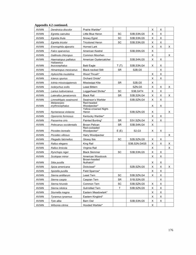
176
Appendix 4.2 continued. AVIAN Dendroica discolor Prairie Warbler* X X AVIAN Egretta caerulea Little Blue Heron SC S3B,S3N,G5 X X AVIAN Egretta thula Snowy Egret SC S3B,S3N,G5 X X AVIAN S3B,S3N,G5 X Egretta tricolor Tricolored Heron SC X AVIAN Eremophila alpestris X X X Horned Lark AVIAN Falco sparverius American Kestrel S3B,S5N,G5 X AVIAN Gallinula chloropus Common Moorhen X X AVIAN Haematopus palliatus atcher S3B,S4N,G5 X X American Oysterc
AVIAN Haliaeetus leucocephalus Bald Eagle T (T) S3B,S3N,G4 X X
AVIAN Himantopus mexicanus d Stilt R S2B,G5 X Black-necke SAVIAN Hylocichla mustelina Wood Thrush* X X AVIAN Icterus spurius Orchard Oriole* X X AVIAN Ictinia mississippiensis Mississippi Kite SR S2B,G5 X AVIAN Ixobrychus exilis X X X Least Bittern SZN,G5 AVIAN Lanius ludovicianus ke* C S3B,G4T4 X X Loggerhead Shri SAVIAN Laterallus jamaicensis Black Rail SR S3B,S2N,G4 X X X AVIAN Limnothlypis swainsonii 4 X X Swainson’s Warbler S3B,SZN,G
AVIAN Melanerpes erythrocephalus
Red-headed Woodpecker* X X
AVIAN Nyctanassa violacea t-
S G5 X X Yellow-crowned NighHeron 3B,SZN,
AVIAN Oporornis formosus Kentucky Warbler* X X AVIAN Passerina ciris Painted Bunting* R S3V,SZN,G4 X X SAVIAN Pelecanus occidentalis S3B,S4N,G4 X Brown Pelican SR
AVIAN Picoides borealis Red-cockaded Woodpecker* E S2,G3 X X (E)
AVIAN ker X Picoides villosus Hairy Woodpec AVIAN X Plegadis falcinellus Glossy Ibis SC S2B,SZN,G5 X AVIAN 5 X X Rallus elegans King Rail S3B,S2N,G4G X AVIAN X Rallus limicola Virginia Rail X AVIAN immer S3B,S3N,G5 X X Rynchops niger Black Sk SCAVIAN ock X Scolopax minor American Woodc X
AVIAN X Sitta pusilla Brown-headed Nuthatch* X
AVIAN S2B,SZN,G5 X X Spiza americana Dickcissel* X AVIAN X Spizella pusilla Field Sparrow* X AVIAN X Sterna antillarum Least Tern SC S3B,SZN,G4 X AVIAN X Sterna caspia Caspian Tern SR S1B,S2N,G5 AVIAN C S3B,SZN,G5 X X Sterna hirundo Common Tern SAVIAN X Sterna nilotica Gull-billed Tern T S3B,SZN,G5 X AVIAN X X Sturnella magna Eastern Meadowlark* AVIAN X Tyrannus tyrannus Eastern Kingbird* X AVIAN S3B,S3N,G5 X Tyto alba Barn Owl X AVIAN Wilsonia citrina Hooded Warbler* X
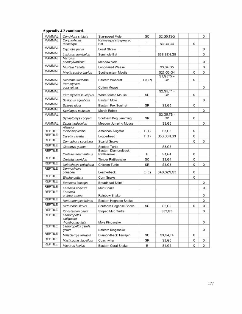
177
L St SC S2,G5, Q X
Appendix 4.2 continued. MAMMA Condylura cristata ar-nosed Mole T2MAMMAL Rafinesque’s Big-eared
Bat T S3,G X Corynorhinus rafinesquii 3,G4
MAMMAL Le X Cryptotis parva ast Shrew MAMMAL lus Se S X Lasiurus semino minole Bat 3B,SZN,G5 MAMMAL
M X Microtus pennsylvanicus eadow Vole
MAMMAL Lo S3,S4,G5 X Mustela frenata ng-tailed Weasel MAMMAL So S X X Myotis austroriparius utheastern Myotis 2?,G3,G4
MAMMAL na Eastern Woodrat TS1,G5T
X Neotoma florida (CP) 5 –
CP MAMMAL
Co X Peromyscus gossypinus tton Mouse
MAMMAL copus W SC
S2,G5, - CP X Peromyscus leu hite-footed Mouse
T1
MAMMAL Ea X Scalopus aquaticus stern Mole MAMMAL Ea rrel SR X Sciurus niger stern Fox Squi S3,G5 MAMMAL M X Sylvilagus palustris arsh Rabbit MAMMAL
Southern Bog Lemming S2,G
X Synaptomys cooperi SR 5,TS -
CP
MAMMAL M X Zapus hudsonius eadow Jumping Mouse S3,G5
REPTILE Am T ) S3,G5 X Alligator mississippiensis erican Alligator (T
REPTILE Lo T ) S3B,S3N,G3 X Caretta caretta ggerhead (TREPTILE Sc X X Cemophora coccinea arlet Snake REPTILE a Sp Clemmys guttat otted Turtle S3,G5 REPTILE Ea k
Ra X Crotalus adamanteus stern Diamondbacttlesnake E S1,G4
REPTILE Ti S X Crotalus horridus mber Rattlesnake SC 3,G4 REPTILE laria Ch SR S3,G X X Deirochelys reticu icken Turtle 5REPTILE
Le E SAB,SZN,G3 X Dermochelys coriacea atherback (E)
REPTILE Co X Elaphe guttata rn Snake REPTILE s Broadhead Skink X Eumeces laticep REPTILE M X Farancia abacura ud Snake REPTILE
Ra X Farancia erytrogramma inbow Snake
REPTILE atirhinos Eastern Hognose Snake X Heterodon pl REPTILE So ose Snake SC X X Heterodon simus uthern Hogn S2,G2 REPTILE rii St S3?,G5 X Kinosternon bau riped Mud Turtle REPTILE
ta M X
Lampropeltis calligaster rhombomacula ole Kingsnake
REPTILE tula Ea X
Lampropeltis gegetula stern Kingsnake
REPTILE in Di SC S3,G4,T4 X Malaclemys terrap amondback Terrapin REPTILE Co S S3,G5 X X Masticophis flagellum achwhip RREPTILE lvius Ea E X X Micrurus fu stern Coral Snake S1,G5
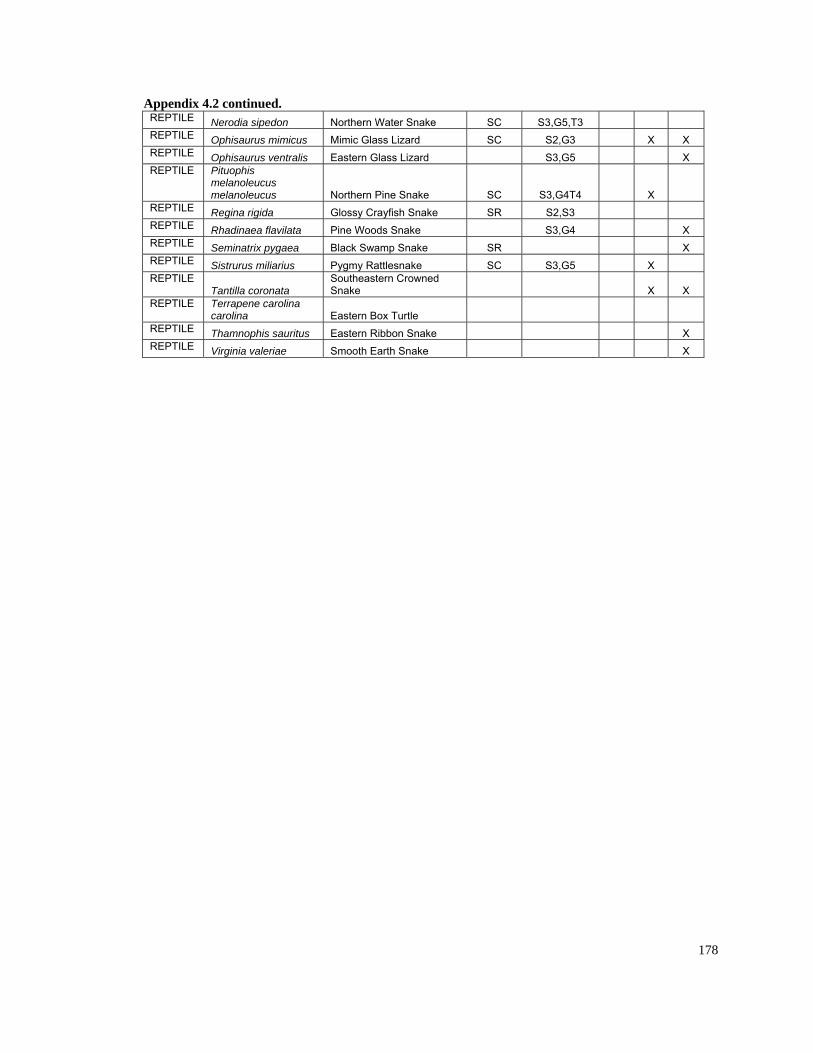
178
ake
Appendix 4.2 continued. REPTILE Nerodia sipedon Northern Water Sn SC S3,G5,T3 REPTILE Ophisaurus mimicus Mimic Glass Lizard SC S2,G3 X X REPTILE Ophisaurus ventralis Eastern Glass Lizard S3,G5 X REPTILE Pituophis
melanoleucus melanoleucus Northern Pine Snake SC S3,G4T4 X
REPTILE Snake SR S2,S3 Regina rigida Glossy Crayfish REPTILE Rhadinaea flavilata Pine Woods Snake S3,G4 X REPTILE Seminatrix pygaea Black Swamp Snake SR X REPTILE Sistrurus miliarius Pygmy Rattlesnake SC S3,G5 X REPTILE
Tantilla coronata Southeastern Crowned Snake X X
REPTILE Terrapene carolina carolina Eastern Box Turtle
REPTILE Thamnophis sauritus n Snake Eastern Ribbo X REPTILE Virginia valeriae Smooth Earth Snake X
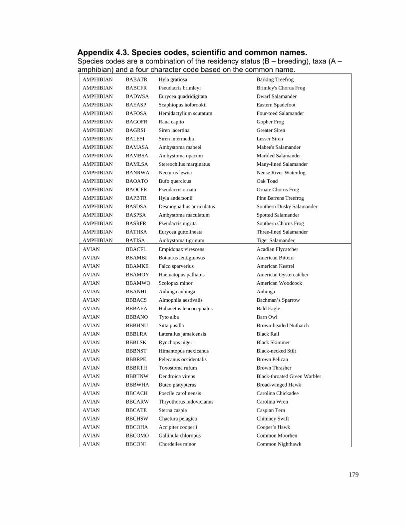
179
cies codes, scientific and common names. s ombination of the residency s s (B ing taxa (A –i ar ed on the mon .
B Hy Barkin
Appendix 4.3. SpeSpecie codes are a c tatu – breed ), amphib an) and a four ch acter code bas com name
AMPHI IAN BABATR la gratiosa g Treefrog AMPHIB R Pseudacris brimleyi Brimley's Chorus Frog IAN BABCFAMPHIB SA Eu Dwar r IAN BADW rycea quadridigitata f SalamandeAMPHIB SP Sc Eastern Spadefoot IAN BAEA aphiopus holbrookii AMPHIB He -toed ander IAN BAFOSA midactylium scutatum Four SalamAMPHIB Ra Gopher Frog IAN BAGOFR na capito AMPHIB Si GreateIAN BAGRSI ren lacertina r Siren AMPHIBIAN BALESI Si Lesser Siren ren intermedia AMPHIB Am mabeei Mabee's S mander IAN BAMASA bystoma alaAMPHIB Am Marbled Salamander IAN BAMBSA bystoma opacum AMPHIB St Many-lined SalamanderIAN BAMLSA ereochilus marginatus AMPHIB A Ne Neuse River Waterdog IAN BANRW cturus lewisi AMPHIBIAN BAOATO Bufo quercicus Oak Toad AMPHIBIAN BAOCFR Pseudacris ornata Ornate Chorus Frog AMPHIBIAN BAPBTR Hyla andersonii Pine Barrens Treefrog AMPHIBIAN BASDSA Desmognathus auriculatus Southern Dusky Salamander AMPHIBIAN BASPSA Ambystoma maculatum Spotted Salamander AMPHIBIAN BASRFR Pseudacris nigrita Southern Chorus Frog AMPHIBIAN BATHSA Eurycea guttolineata Three-lined Salamander AMPHIBIAN BATISA Ambystoma tigrinum Tiger Salamander
AVIAN BBACFL Empidonax virescens Acadian Flycatcher AVIAN BBAMBI Botaurus lentiginosus American Bittern AVIAN BBAMKE Falco sparverius American Kestrel AVIAN BBAMOY Haematopus palliatus American Oystercatcher AVIAN BBAMWO Scolopax minor American Woodcock AVIAN BBANHI Anhinga anhinga Anhinga AVIAN BBBACS Aimophila aestivalis Bachman’s Sparrow AVIAN BBBAEA Haliaeetus leucocephalus Bald Eagle AVIAN BBBANO Tyto alba Barn Owl AVIAN BBBHNU Sitta pusilla Brown-headed Nuthatch AVIAN BBBLRA Laterallus jamaicensis Black Rail AVIAN BBBLSK Rynchops niger Black Skimmer AVIAN BBBNST Himantopus mexicanus Black-necked Stilt AVIAN BBBRPE Pelecanus occidentalis Brown Pelican AVIAN BBBRTH Toxostoma rufum Brown Thrasher AVIAN BBBTNW Dendroica virens Black-throated Green Warbler AVIAN BBBWHA Buteo platypterus Broad-winged Hawk AVIAN BBCACH Poecile carolinensis Carolina Chickadee AVIAN BBCARW Thryothorus ludovicianus Carolina Wren AVIAN BBCATE Sterna caspia Caspian Tern AVIAN BBCHSW Chaetura pelagica Chimney Swift AVIAN BBCOHA Accipiter cooperii Cooper’s Hawk AVIAN BBCOMO Gallinula chloropus Common Moorhen AVIAN BBCONI Chordeiles minor Common Nighthawk
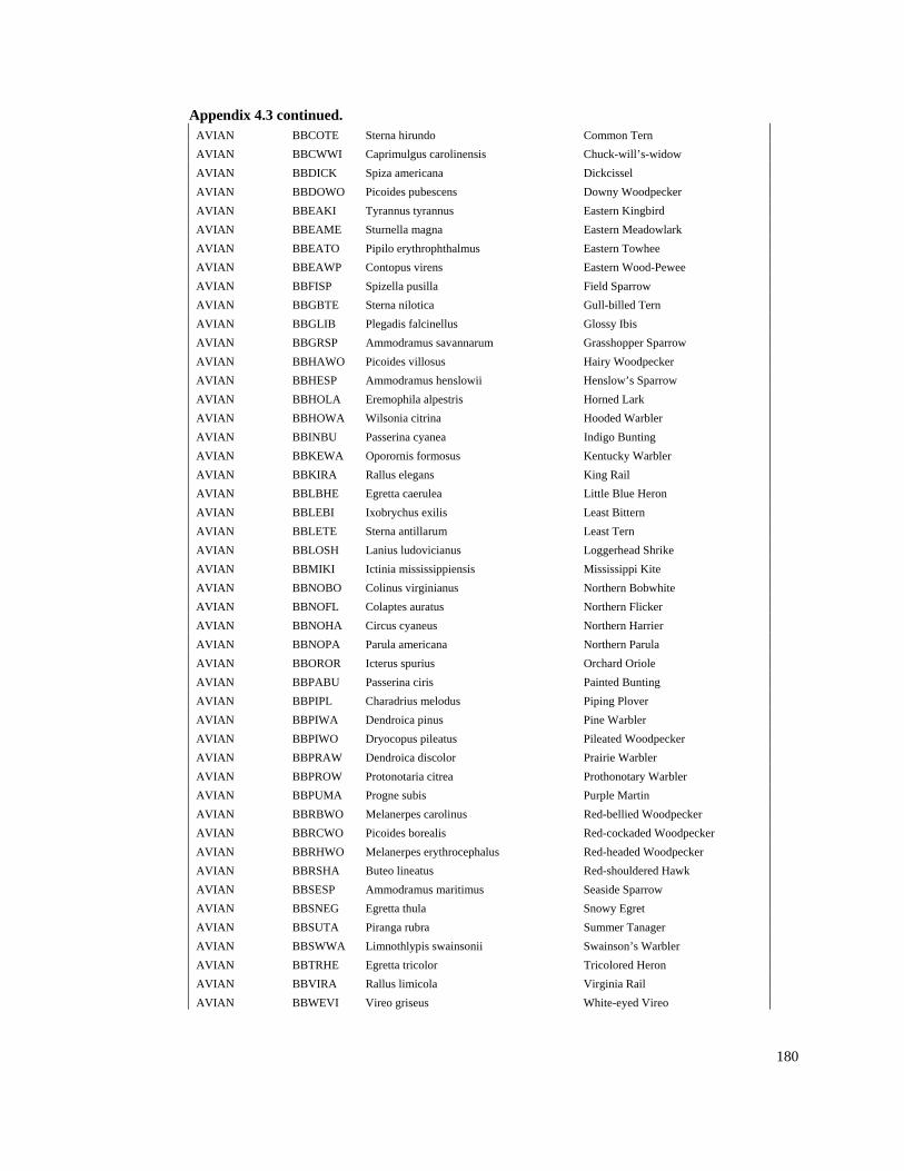
180
Appendix 4.3 continued. AVIAN BBCOTE Sterna hirundo Common Tern AVIAN BBCWWI Caprimulgus carolinensis Chuck-will’s-widow AVIAN BBDICK Spiza americana Dickcissel AVIAN BBDOWO Picoides pubescens Downy Woodpecker AVIAN BBEAKI Tyrannus tyrannus Eastern Kingbird AVIAN BBEAME lark Sturnella magna Eastern MeadowAVIAN BBEATO Pipilo erythrophthalmus Eastern Towhee AVIAN BBEAWP ens Pewee Contopus vir Eastern Wood-AVIAN BBFISP la w Spizella pusil Field SparroAVIAN BBGBTE Tern Sterna nilotica Gull-billed AVIAN BBGLIB Plegadis falcinellus Glossy Ibis AVIAN BBGRSP nnarum w Ammodramus sava Grasshopper SparroAVIAN BBHAWO Picoides villosus Hairy Woodpecker AVIAN BBHESP Ammodramus henslowii Henslow’s Sparrow AVIAN BBHOLA pestris ark Eremophila al Horned LAVIAN BBHOWA Wilsonia citrina Hooded Warbler AVIAN BBINBU ea Passerina cyan Indigo Bunting AVIAN BBKEWA Oporornis formosus Kentucky Warbler AVIAN BBKIRA Rallus elegans King Rail AVIAN BBLBHE Egretta caerulea Little Blue Heron AVIAN BBLEBI Ixobrychus exilis Least Bittern AVIAN BBLETE Sterna antillarum Least Tern AVIAN e BBLOSH Lanius ludovicianus Loggerhead ShrikAVIAN sis BBMIKI Ictinia mississippien Mississippi KiteAVIAN anus ite BBNOBO Colinus virgini Northern BobwhAVIAN BBNOFL Colaptes auratus Northern Flicker AVIAN BBNOHA Circus cyaneus Northern Harrier AVIAN A a Parula BBNOP Parula american NorthernAVIAN R BBORO Icterus spurius Orchard Oriole AVIAN unting BBPABU Passerina ciris Painted BAVIAN us melodus lover BBPIPL Charadri Piping PAVIAN pinus BBPIWA Dendroica Pine Warbler AVIAN oodpecker BBPIWO Dryocopus pileatus Pileated WAVIAN olor r BBPRAW Dendroica disc Prairie WarbleAVIAN rbler BBPROW Protonotaria citrea Prothonotary WaAVIAN A BBPUM Progne subis Purple MartinAVIAN O linus BBRBW Melanerpes caro Red-bellied Woodpecker AVIAN s BBRCWO Picoides boreali Red-cockaded Woodpecker AVIAN rocephalus ecker BBRHWO Melanerpes eryth Red-headed WoodpAVIAN awk BBRSHA Buteo lineatus Red-shouldered HAVIAN ow BBSESP Ammodramus maritimus Seaside SparrAVIAN t BBSNEG Egretta thula Snowy EgreAVIAN ger BBSUTA Piranga rubra Summer TanaAVIAN A ainsonii arbler BBSWW Limnothlypis sw Swainson’s WAVIAN BBTRHE Egretta tricolor Tricolored Heron AVIAN BBVIRA Rallus limicola Virginia Rail AVIAN BBWEVI Vireo griseus White-eyed Vireo
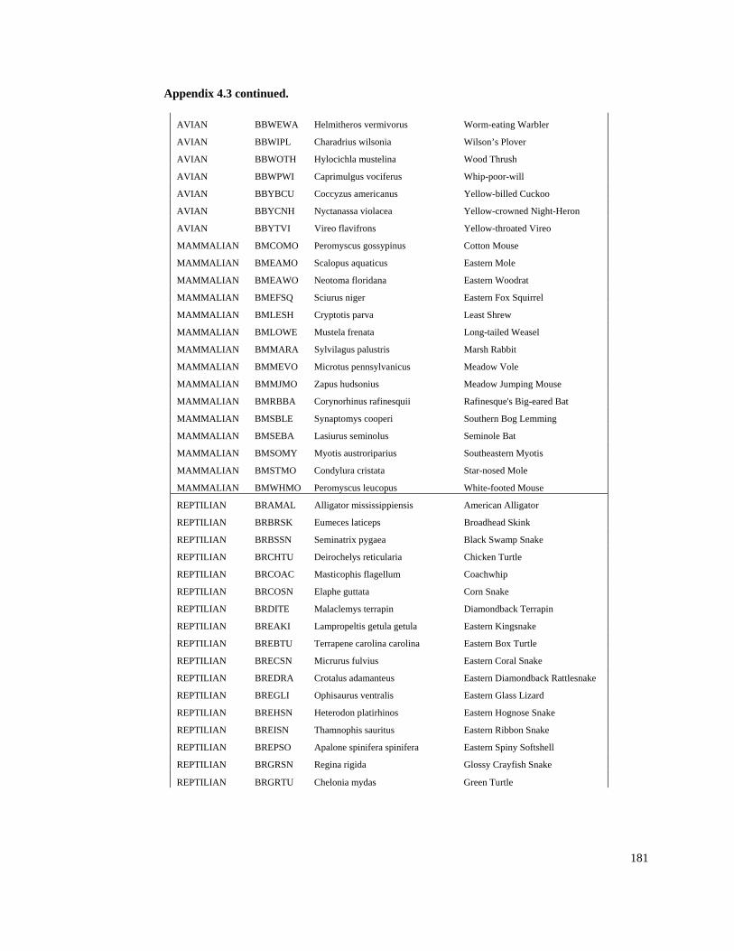
181
.
N WA us W
Appendix 4.3 continued
AVIA BBWE Helmitheros vermivor orm-eating Warbler
AVIAN BBWIPL ilsonia W er Charadrius w ilson’s Plov
AVIAN H elina WBBWOT Hylocichla must ood Thrush
AVIAN BBWPWI ciferus W Caprimulgus vo hip-poor-will
AVIAN Yellow-billed CucBBYBCU Coccyzus americanus koo
AVIAN H Y eron BBYCN Nyctanassa violacea ellow-crowned Night-H
AVIAN TVI Yellow-throated Vireo BBY Vireo flavifrons
MAMMALIAN MO s gossypinus C BMCO Peromyscu otton Mouse
MAMMALIAN MO us E BMEA Scalopus aquatic astern Mole
MAMMALIAN WO E BMEA Neotoma floridana astern Woodrat
MAMMALIAN Q E BMEFS Sciurus niger astern Fox Squirrel
MAMMALIAN SH L BMLE Cryptotis parva east Shrew
MAMMALIAN WE Long-BMLO Mustela frenata tailed Weasel
MAMMALIAN ARA lustris M BMM Sylvilagus pa arsh Rabbit
MAMMALIAN VO lvanicus M BMME Microtus pennsy eadow Vole
MAMMALIAN JMO onius M ping Mouse BMM Zapus huds eadow Jum
MAMMALIAN BA s rafinesquii R d Bat BMRB Corynorhinu afinesque's Big-eare
MAMMALIAN LE ooperi So mming BMSB Synaptomys c uthern Bog Le
MAMMALIAN BA nolus Se BMSE Lasiurus semi minole Bat
MAMMALIAN MY us So BMSO Myotis austroripari utheastern Myotis
MAMMALIAN O StarBMSTM Condylura cristata -nosed Mole
MAMMALIAN M eucopus W BMWH O Peromyscus l hite-footed Mouse
REPTILIAN AL ssissippiensis ABRAM Alligator mi merican Alligator
REPTILIAN K eps BBRBRS Eumeces latic roadhead Skink
REPTILIAN N pygaea B e BRBSS Seminatrix lack Swamp Snak
REPTILIAN TU s reticularia Chicken BRCH Deirochely Turtle
REPTILIAN OAC ellum Coachwhip BRC Masticophis flag
REPTILIAN BRCOSN Elaphe guttata Corn Snake
REPTILIAN E rapin DiamBRDIT Malaclemys ter ondback Terrapin
REPTILIAN I etula getula EBREAK Lampropeltis g astern Kingsnake
REPTILIAN U carolina carolina Eastern Box Turtle BREBT Terrapene
REPTILIAN N EBRECS Micrurus fulvius astern Coral Snake
REPTILIAN A anteus E ke BREDR Crotalus adam astern Diamondback Rattlesna
REPTILIAN I EBREGL Ophisaurus ventralis astern Glass Lizard
REPTILIAN SN platirhinos EBREH Heterodon astern Hognose Snake
REPTILIAN N EaBREIS Thamnophis sauritus stern Ribbon Snake
REPTILIAN O inifera spinifera Eastern Spiny Softshell BREPS Apalone sp
REPTILIAN N GBRGRS Regina rigida lossy Crayfish Snake
REPTILIAN TU das GBRGR Chelonia my reen Turtle
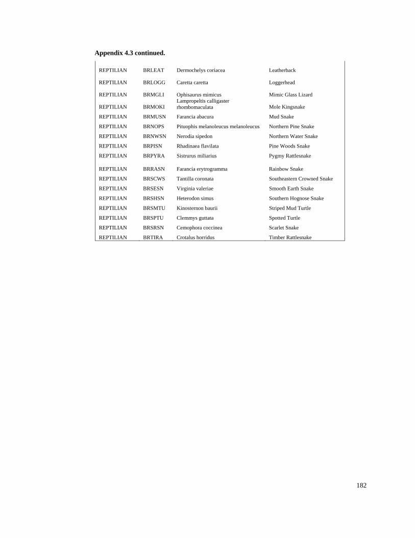
Appendix 4.3 continued.
182
N REPTILIA BRLEAT Dermochelys coriacea Leatherback
REPTILIAN BRLOGG Caretta caretta Loggerhead
RE AN BRM izard PTILI GLI Ophisaurus mimicus Mimic Glass L
REPTILIAN BRMOKI Lampropeltis calligaster rhombomaculata Mole Kingsnake
REPTILIAN BRMUSN Farancia abacura Mud Snake
REPTILIAN eucus melanoleucus BRNOPS Pituophis melanol Northern Pine Snake
REPTILIAN BRNWSN Nerodia sipedon Northern Water Snake
REPTILIAN BRPISN Rhadinaea flavilata Pine Woods Snake
REPTILIAN BRPYRA Sistrurus miliarius Pygmy Rattlesnake
REPTILIAN BRRASN Farancia erytrogramma Rainbow Snake
REPTILIAN BRSCWS Tantilla coronata Southeastern Crowned Snake
REPTILIAN BRSESN Virginia valeriae Smooth Earth Snake
REPTILIAN BRSHSN Heterodon simus Southern Hognose Snake
REPTILIAN BRSMTU Kinosternon baurii Striped Mud Turtle
REPTILIAN BRSPTU Clemmys guttata Spotted Turtle
REPTILIAN BRSRSN Cemophora coccinea Scarlet Snake
REPTILIAN BRTIRA Crotalus horridus Timber Rattlesnake