Outlier Detection Using the Smallest Kernel

Principal Components

Alan J. Izenman and Yan Shen

The smallest principal components have not attracted much attention in the

statistics literature. This apparent lack of interest is due to the fact that, compared

with the largest principal components that contain most of the total variance in

the data, the smallest principal components only contain the noise of the data and,

therefore, appear to contribute minimal information. However, because outliers are

a common source of noise, the smallest principal components should be useful for

outlier detection. This article proposes a new and novel method for outlier detection

using the smallest kernel principal components in a feature space induced by the

radial basis function kernel. We show that the eigenvectors corresponding to the

smallest kernel principal components can be viewed as those for which the residual

sum of squares is minimized, and we use those components to identify outliers based

upon a simple graphical technique. A threshold between “large” and “small” kernel

principal components is proposed in this paper, and a nonparametric method for

locating the smallest kernel principal component is suggested. Simulation studies

show that under a univariate outlier situation, the proposed method is as good as

the best method available, and real-data examples also suggest that this method is

often better.

KEY WORDS: Kernel methods; Kernel principal component analysis; Mahalanobis

distance; Multivariate outlier detection; Principal component analysis.

Authors’ Footnote

Alan J. Izenman is Professor of Statistics in the Department of Statistics, and

Director of the Center for Statistical and Information Science, Office of the Vice-

President for Research and Graduate Studies, Temple University, Philadelphia, PA

19122 (E-mail: alan@temple.edu). Yan Shen is biostatistician in the Department

of Biometrics and Clinical Informatics at Johnson and Johnson Pharmaceutical Re-

search & Development, L.L.C., New Jersey, NJ 08869 (E-mail: yshen10@prdus.jnj.com).

2

1. INTRODUCTION

Principal component analysis (PCA), first introduced by Hotelling (1933), is a

well-established dimension-reduction method. It replaces a set of correlated vari-

ables by a smaller set of uncorrelated linear combinations of those variables, such

that these linear combinations explain most of the total variance. It is also a way

of identifying inherent patterns, relations, regularities, or structure in the data. Be-

cause such patterns are difficult to detect in high-dimensional data, PCA can be a

powerful tool.

As a linear statistical technique, PCA cannot accurately describe all types of

structures in a given dataset, specially nonlinear structures. Kernel principal com-

ponent analysis (KPCA) has recently been proposed as a nonlinear extension of

PCA (Scholkopf, Smola, and Muller, 1998). See also Scholkopf and Smola (2002).

Kernel methods were introduced into the computer science literature specifically for

pattern analysis (see, e.g., Shawe-Taylor and Cristianini, 2004). These are pow-

erful techniques, which have been applied to many types of statistical methods,

including support vector machines, canonical correlation analysis, and independent

component anaysis.

KPCA maps the data from the original space into a feature space via a non-

linear transformation, and then performs linear PCA on the mapped data. The

principal components (PCs) found by this process are called kernel principal com-

ponents (KPCs). In pattern analysis, a feature space is an abstract space where

each transformed sample is represented as a point in n-dimensional space. Because

the feature space could be of very high dimension, possibly even infinite dimen-

sional, kernel methods employ inner-products instead of carrying out the mapping

explicitly. Mercer’s theorem of functional analysis (Mercer, 1909) states that if k is

a continuous kernel of a positive integral operator, we can construct a mapping into

3

a space where k acts as an inner-product.

Much of the linear PCA literature (and also that of KPCA) has been focused

primarily on the largest few PCs because they account for most of the variation in

the data, as opposed to the smallest PCs, which account for only the noise in the

data. Yet, outliers can be viewed as a common source of noise. In this article, we

study a new approach to multivariate outlier detection using the smallest KPCs. We

show that the eigenvectors corresponding to the smallest KPCs can be viewed as

those for which the residual sum of squares is minimized, and we propose a threshold

(or cutoff) value, which distinguishes “large” from “small” KPCs. A nonparametric

method is suggested to determine the location of the smallest KPC. We can then

detect outliers easily by plotting the smallest KPC against the second smallest KPC.

We show that this approach is competitive with (and often an improvement over)

existing methods.

The remainder of this article is organized as follows. In Section 2, we introduce

the necessary background on linear PCA and KPCA. We then present in Section

3 the proposed outlier detection method in detail. Numerical results are given in

Section 4, using both simulated data and real-data examples, and conclusions are

drawn in Section 5.

2. PCA AND KPCA

2.1 Principal Component Analysis

Given a p-vector, x = (x1, ..., xp)τ , in input space X , PCA finds uncorrelated

linear combinations of the p variables such that fewer than p of these combina-

tions contain most of the variation in the data. Assume that x has zero mean

and (p × p) covariance matrix Σ, whose eigenvalue-eigenvector pairs are given by

4

(µ1,u1), (µ2,u2), . . . , (µp,up), where µ1 ≥ µ2 ≥ · · · ≥ µp ≥ 0. Then,

ξ1 = uτ1x, ξ2 = uτ

2x, . . . , ξp = uτpx, (1)

are the p PCs, where

varξi = uτi Σui = µi and covξi, ξj = uτ

i Σuj = 0, j < i. (2)

Note that in (1) and (2), uτ is the transpose of the column-vector u. Principal

component analysis orthogonalizes the covariance matrix Σ into a maximum of p

PCs. The first PC is the linear combination of the variables that explains the

greatest amount of the total variation in x. The second PC is the linear combination

of the variables that explains the next largest amount of variation and is uncorrelated

with the first PC, and so on. If the first l (say, three) components contain most of

the total variation (say, 90%), then the original variables can be replaced by these

components without too much loss of variance information. The coefficients of the

PCs (i.e., the elements of the ξs) can be derived through least-squares optimization

or by the use of Lagrangian multipliers. For details, see Izenman (2008, Section

7.2).

2.2 Kernel PCA

Instead of reducing the dimensionality directly in the original space, KPCA works

in a higher-dimensional feature space by forming inner-products of a transformation

function Φ. A mapping is performed through Φ : Rp → H, where the original data

lie in Rp and the features lie in a Hilbert space H. The transformation Φ is usually

nonlinear, but the remarkable thing is that it does not have to be specified explic-

itly. By Mercer’s theorem, under suitable conditions of nonnegative-definiteness,

the feature space H induced by the kernel function,

k(x,y) = 〈Φ(x),Φ(y)〉, (3)

5

exists and can be constructed from eigenfunctions and positive eigenvalues.

Assume that the data in feature space are centered; that is,∑n

i=1 Φ(xi) = 0.

Then, the estimated covariance matrix is Ω = 1n

∑ni=1 Φ(xi)Φ(xi)

τ . To find KPCs

in this feature space, we solve the eigenequations, λv = Ωv, for nonzero eigenval-

ues λ and corresponding eigenvectors v. Note that all solutions v with λ 6= 0 lie

in the span of Φ(x1), . . . ,Φ(xn). This implies that (1) the eigenequations can be

written as λ〈Φ(xi),v〉 = 〈Φ(xi),Ωv〉, i = 1, 2, . . . , n, and (2) there exist coefficients

αi, i = 1, 2, . . . , n, such that v =∑n

i=1 αiΦ(xi). This enables us to rewrite the

eigenequations as

λn∑

i=1

αi〈Φ(xk), Φ(xi)〉 =1

n

n∑

i=1

αi

⟨

Φ(xk),n∑

j=1

Φ(xj)⟨

Φ(xj),Φ(xi)⟩

⟩

, (4)

which, in matrix form, becomes nλKα = K2α, where K = (Kij), Kij = 〈Φ(xi),Φ(xj)〉,is an (n× n) Gram matrix, and α = (α1, ..., αn)τ .

Because K is symmetric, it has a set of eigenvectors that spans the whole space.

Thus, nλα = Kα gives all solutions α of the eigenvectors and nλ of the eigenvalues.

For the sake of simplicity, let λi represent the eigenvalues of K equivalent to nλi,

where λ1 ≥ λ2 · · · ≥ λl, with λl being the last nonzero eigenvalue, and α1, . . . ,αl

the corresponding eigenvectors. We normalize the α1, ...,αl by requiring that the

corresponding vectors in H be normalized, i.e., 〈vk,vk〉 = 1, k = 1, 2, . . . , l. This

can be translated into a normalization condition for α1, ...,αl:

1 =n∑

i,j=1

αki α

kj 〈Φ(xi),Φ(xj)〉 =

n∑

i,j=1

αki α

kjKij = 〈αk,Kαk〉 = λk〈αk,αk〉. (5)

For a point x in the original space Rp with an image Φ(x) in the feature space H,

the projection

〈vk,Φ(x)〉 =1√λk

n∑

i=1

αki 〈Φ(xi),Φ(x)〉 (6)

can be called its kth KPC corresponding to Φ, k = 1, 2, . . . , l.

6

In practice, we cannot assume that the points in feature space have mean zero.

Therefore, we subtract n−1∑ni=1 Φ(xi) from all points. This leads to a minor change

of the Gram matrix K, namely K∗ = HKH, where H = In −n−1Jn is the centering

matrix, Jn = 1n1τn, and 1n is an n-vector of all ones.

3. OUTLIER DETECTION USING THE SMALLEST PRINCIPAL

COMPONENTS

The earliest work that incorporates the smallest PCs occurs in Gnanadesikan and

Wilk’s (1966, 1968) generalization of PCA to the nonlinear case. Building upon these

ideas, Gnanadesikan and Kettenring (1972) state that “with p-dimensional data, the

projection onto the ‘smallest’ principal component would be relevant for studying

the deviation of an observation from a hyperplane of closest fit, while the projections

on the ‘smallest’ q principal component coordinates would be relevant for studying

the deviation of an observation from a fitted linear subspace of dimensionality p−q.”See also Gnanadesikan (1977, Section 2.4.2).

More recently, Donnell, Buja and Stuetzle (1994) introduced the concept of “ad-

ditive principal components” (APCs) to help identify additive dependencies and

concurvities among the predictor variables in a regression model. The smallest ad-

ditive principal component is defined as an additive function of the data,∑

i φi(xi),

with smallest variance. The function φi is usually nonlinear and may be different

for each xi. If the φis are linear and identical, then the problem reduces to standard

PCA. They outlined some analytical methods for theoretical calculations of APCs,

and showed that by plotting the last few smallest APCs against the raw variables,

they could discover any existing nonlinear dependencies between those variables.

Our approach is different from these authors in that we use the kernel function

k to transform the data from input space to feature space, and then apply standard

7

PCA to find the smallest KPCs in that space. From Section 2, we know that if the

kernel functions satisfy Mercer’s conditions, we are doing a standard PCA in feature

space. Consequently, all mathematical and statistical properties of PCA carry over

to KPCA (Scholkopf and Smola, 2002).

3.1 Definitions

We characterize the smallest KPC by extending a definition of the smallest PC.

For the smallest KPC, vn is the eigenvector corresponding to the smallest eigenvalue

of the eigenequation λv = Ωv. Because Φ is usually unknown, we are unable to

calculate Ω directly and solve for vn. Instead, we replace v by∑n

i=1 αiΦ(xi) in an

equivalent eigenequation λ〈Φ(xi),v〉 = 〈Φ(xi),Ωv〉. Hence, in this characterization,

we need to find αn, the eigenvector corresponding to the smallest eigenvalue λn of

the eigenequation nλα = Kα.

KPCA could find up to n non-zero distinct KPCs. However, in practice, when

n is large, eigenvalues equal to or approximately equal to 0 are likely to occur, so

that the corresponding KPCs contain almost no information, even about the noise.

Therefore, finding the smallest KPC is not a trivial task. Hence, we will use the

notation vl(αl) instead of vn(αn) to represent the eigenvector corresponding to the

smallest eigenvalue of the eigenequation, where l needs to be determined. Now we

are ready to define the smallest KPC.

Definition 1. In a feature space properly defined through a kernel function k, the

smallest kernel principal component is a random vector φl =∑n

i,j=1 αli〈Φ(xi),Φ(xj)〉,

which has smallest variance subject to λl〈αl,αl〉 = 1, where αl is the eigenvector

corresponding to the smallest non-zero eigenvalue λl of the eigenequation nλα =

Kα, K = (Kij), and Kij = 〈Φ(xi),Φ(xj)〉 = k(xi,xj).

Analogously, we can define the smallest KPCs with the additional constraint

8

that they are mutually uncorrelated.

Definition 2. In a feature space properly defined through a kernel function k,

the mth-smallest kernel principal component is a random vector

φ(m) =n∑

i,j=1

α(m)i 〈Φ(xi),Φ(xj)〉 (7)

with smallest variance, subject to the constraints

λ(m)〈α(m),α(m)〉 = 1, Cov(φ(m),φ(t)) = 0, t = m− 1, m− 2, . . . , 1. (8)

Here, α(m) is the eigenvector corresponding to the mth-smallest non-zero eigenvalue

λ(m) of the eigenequation nλα = Kα, and Kij = 〈Φ(xi),Φ(xj)〉 = k(xi,xj).

Both PCA and KPCA boil down to eigenproblems. Therefore, to understand

the use of the smallest KPCs, we study their eigenproperties.

3.2 Eigenvectors Corresponding to

the Smallest KPCs

The Gram matrix K is the matrix whose elements are the inner-products of

the mapped data; K is symmetric and nonnegative-definite if the kernel function

k satisfies Mercer’s conditions. For the sake of simplicity, let K = XXτ , where

X = (x1, · · · ,xn) is the (p×n) data matrix whose ith column xi ∈ X , i = 1, 2, . . . , n.

We start with the singular value decomposition of X = UDVτ , where U and

V are orthonormal matrices and D is a diagonal matrix containing singular values

in descending order of magnitude. We represent K as K = XXτ = UΛUτ , where

Λ = D2. Alternatively, we can construct a matrix K∗ = XτX = VΛVτ , with the

same eigenvalues as K. By the Courant–Fischer Min-Max Theorem (McDiarmid,

1989) and the definition of a projection operator, the first (or largest) eigenvalue of

9

K is given by

λ1(K) = max06=α∈Rn

ατK∗α

ατα

= max06=α∈Rn

ατXτXα

ατα

= max06=α∈Rn

‖Xα‖2

ατα

= max06=α∈Rn

n∑

i=1

‖Pα(xi)‖2

=n∑

i=1

‖xi‖2 − min06=α∈Rn

n∑

i=1

‖Pα(xi)‖2, (9)

where Pα(x) is the projection of x onto the space spanned by α, and Pα(x) is the

projection of x onto the space perpendicular to α. Equation (9) suggests that the

first eigenvector can be characterized as the direction for which the residual sum of

squares is minimized. Applying the same line of reasoning to the general form of

the Courant-Fischer Min-Max Theorem, the mth eigenvalue of K can be expressed

as

λm(K) = maxdim(T )=m

min06=α∈T

n∑

i=1

‖Pα(xi)‖2, (10)

which implies that if αm is the mth eigenvector of K∗, then

λm(K) =n∑

i=1

‖Pαm(xi)‖2. (11)

Consequently, if Tm is the space spanned by the first m eigenvectors, then

m∑

j=1

λj(K) =n∑

i=1

‖PTm(xi)‖2 =

n∑

i=1

‖xi‖2 −n∑

i=1

‖PTm(xi)‖2

. (12)

By induction over the dimension of T , it readily follows that we can characterize

the sum of the first m and the sum of the last (n−m) eigenvalues by

m∑

j=1

λj(K) = maxdim(T )=m

n∑

i=1

‖PT (xi)‖2 =n∑

i=1

‖xi‖2 − mindim(T )=m

n∑

i=1

‖PT (xi)‖2, (13)

10

n∑

j=m+1

λj(K) =n∑

i=1

‖xi‖2 −m∑

j=1

λj(K) = mindim(T )=m

n∑

i=1

‖PT (xi)‖2, (14)

respectively. Hence, when m = n − 1, it implies that the subspace spanned by the

last eigenvector is characterized as that for which the residual sum of squares is

minimized.

We can now generalize all of the above into a kernel-defined feature space by

replacing every vector x by Φ(x), where Φ is the corresponding feature map, and

K = (Kij), where Kij = 〈Φ(xi),Φ(xj)〉, is the Gram matrix. Because the solution of

KPCA is achieved by the eigendecomposition of K, the interpretation of the smallest

KPC has much in common with the analysis of residuals.

Consider the kernel operator K(f) and its eigenspace. The kernel operator is

defined as

K(f)(x) =∫

Xk(x, z)f(z)p(x)dz, (15)

where p(x) is the underlying probability density function in input space and K(f) is a

linear operator for the function f . Assuming the operator K is nonnegative-definite,

by Mercer’s Theorem, we can decompose k(x, z) as a sum of eigenfunctions,

k(x, z) =∞∑

i=1

λiψi(x)ψi(z) = 〈Φ(x),Φ(z)〉, (16)

where λi = λi(K(f)) are the eigenvalues of K(f). The functions

ψ(x) = (ψ1(x), . . . , ψi(x), . . . ) (17)

form a complete orthonormal basis with respect to the inner-product, 〈f, g〉 =∫

X f(x)g(x)p(x)dx, and Φ(x) is the feature space mapping,

Φ : x → φi(x) =√

λiψi(x) ∈ H, i = 1, 2, . . . . (18)

Note that ψi(x) has norm 1; that is,∫

X ψi(x)ψj(x)p(x)dx = δij, where δij = 1 if

i = j, and 0 otherwise. Also, ψi(x) satisfies ψi(x) = 1λi

∫

X k(x, z)ψi(z)p(z)dz, so

11

that∫

X×Xk(x, z)ψi(x)ψi(z)p(x)p(z)dxdz = λi. (19)

For a general function g(x), we define the vector g =∫

X g(x)ψ(x)p(x)dx. Then,

the expected squared-norm of the projection of Φ(x) onto the vector g is given by

E[

‖Pg(Φ(x))‖2]

=∫

X‖Pg(Φ(x))‖2

p(x)dx

=∫

X(gτ Φ(x))2

p(x)dx

=∫

X

∫

X

∫

X

[

g(y)ψ(y)τΦ(x)p(y)dy][

g(z)ψ(z)τΦ(x)p(z)dz]

p(x)dx

=∫

X×X×Xg(y)g(z) ×

∞∑

i =1

√

λiψi(y)ψi(x)p(y)dy

∞∑

j=1

√

λjψj(z)ψj(x)p(z)dz

p(x)dx

=∫

X×Xg(y)g(z) ×

∞∑

i,j=1

√

λiψi(y)p(y)dy√

λjψj(z)p(z)dz

∫

Xψi(x)ψj(x)p(x)dx

=∫

X×Xg(y)g(z)

[

∞∑

i=1

λiψi(y)ψi(z)

]

p(y)dyp(z)dz

=∫

X×Xg(y)g(z)k(y, z)p(y)dyp(z)dz. (20)

The sum of the finite-case characterization of eigenvalues and eigenvectors (19) can,

therefore, be replaced by the expectation,

λm(K(f)) = maxdim(T )=m

min06=α∈T

E[

‖Pα(Φ(x))‖2]

. (21)

Similarly, the sum of the first m and sum of the last (n − m) eigenvalues can be

expressed as

m∑

j=1

λj(K(f)) = maxdim(T )=m

E[

‖PT (Φ(x))‖2]

12

= E[

‖Φ(x)‖2]

− mindim(T )=m

E[

‖PT (Φ(x))‖2]

, (22)

n∑

j=m+1

λj(K(f)) = E[

‖Φ(x)‖2]

−m∑

j=1

λj(K(f))

= mindim(T )=m

E[

‖PT (Φ(x))‖2]

, (23)

where PT (Φ(x)) is the projection of Φ(x) onto the subspace T , and PT (Φ(xi)) is

the projection of Φ(x) onto the space orthogonal to T . The above results again

imply that, in the feature space induced by the map Φ, the smallest KPC can be

interpreted in a similar way as that of residuals.

3.3 Threshold between Small and Large Kernel

Principal Components

The eigenvalues are bounded below by 0 because K is nonnegative-definite. The

existence of an eigenvalue equal to 0 indicates degeneracy or nonlinear dependency.

In practice, exact 0 rarely happens due to computational accuracy, but near-zero or

duplicates of near-zero eigenvalues usually exist, especially when n is large. There-

fore, we have to determine the magnitude of the smallest eigenvalues so that they do

contain important information about the noise. Meanwhile, because our attention

is focused on the smallest KPCs, we need a clear separation between “large” and

“small” KPCs.

Intuitively, we could do this by separating the eigenvalues corresponding to the

“large” and “small” KPCs. However, for a given dataset, applying different kernels

leads to different kernel matrices that need to be eigendecomposed and, hence,

generate different eigenstructures. For example, when applying a polynomial kernel,

k(x, z) = (〈x, z〉 + c)d, the magnitudes of the eigenvalues increase along with the

increase of the power d. Hence, a universal threshold (with respect to all kernel

functions) to separate “large” from “small” KPCs is impossible. Therefore, we have

13

to enforce some restrictions on the kernel functions being chosen.

We consider only kernel functions that represent probability measures or empir-

ical distributions, for then the eigenvalues derived from those kernels are bounded

above. In particular, we use a Gaussian radial basis function (RBF) kernel,

Kij = exp

(

−‖xi − xj‖2

2σ2

)

, σ > 0, (24)

where the matrix K = (Kij) induced by the RBF kernel (24) has full rank. Define

a vector space by taking a linear combination of the form,

f(·) =n∑

i=1

αik(·,xi). (25)

Next, define an inner-product between f and another function g as

〈f, g〉 =n∑

i=1

m∑

j=1

αiβjk(xi,yj), (26)

where

g(·) =m∑

j=1

βjk(·,yj). (27)

Here, n and m are integers, αi, βj ∈ R, and xi,yj ∈ X , i = 1, 2, . . . , n, j =

1, 2, . . . , m. Expression (26) explicitly contains the expansion coefficients, which

need not be unique. To see that the inner-product is nevertheless well-defined, note

that 〈f, g〉 =∑m

j=1 βjf(yj), using k(yj,xi) = k(xi,yj). The sum in (26), how-

ever, does not depend on the particular expansion of f . Similarly, for g, 〈f, g〉 =∑n

i=1 αig(xi). Thus, 〈·, ·〉 is symmetric and nonnegative-definite, 〈f, g〉 = 〈g, f〉,〈f, f〉 =

∑ni,j=1 αiαjk(xi,xj) ≥ 0, and, hence, is bilinear. Thus, the space H is

a vector space and is endowed with an inner-product. We turn the space H into

a Hilbert space by completing it in the norm corresponding to the inner-product,

‖f‖ =√

〈f, f〉, where “completeness” means that every Cauchy sequence of elements

in the space converges to an element in the space, in the sense that the norm of dif-

ferences approaches zero. The constraint of the smallest KPC optimization problem

14

can now be cast as a restriction to the unit ball in H: varΦ(x) = ‖Φ(x)‖2 = 1. It

follows from an elementary theorem in L2 theory that there exists a bounded, sym-

metric, linear operator P on H such that the optimization problem for the smallest

KPC can be written as:

minH

〈Φ(x),PΦ(x)〉, subject to ‖Φ(x)‖2 = 1. (28)

We need to identify the operator P that satisfies these conditions.

Lemma 1. Define the operator P : H → H by the component mappings

(PΦ(x))i = PiΦ(xj), i, j = 1, 2, . . . , n, (29)

where Pi is the orthogonal projection onto the subspace Hi of the feature space H.

Then, P is symmetric, nonnegative-definite, and bounded above by n.

Proof. The operator P is nonnegative:

〈Φ(x),PΦ(x)〉 =∑

i,j

⟨

Φ(xi),PiΦ(xj)⟩

=∑

i,j

⟨

Φ(xi),Φ(xj)⟩

=⟨

∑

i

Φ(xi),∑

j

Φ(xj)⟩

=∥

∥

∥

∑

i

Φ(xi)∥

∥

∥

2

≥ 0,

and P is bounded above by n:

‖PΦ(x)‖2 =∑

i

‖PiΦ(xj)‖2 ≤∑

i

‖Φ(xj)‖2 = n‖Φ(xj)‖2 = n.

The eigencharacterization of the smallest KPC now follows from standard results

about symmetric operators. Because we are working in a possibly-infinite Hilbert

15

space, the existence of the smallest eigenvalue of P is not guaranteed. Therefore,

we use the phrase “if it exists” whenever necessary.

Proposition 1. The eigenvector corresponding to the smallest eigenvalue of the

operator P, if it exists, is the vector for the smallest KPC.

Proposition 2. The eigenvector corresponding to the mth smallest eigenvalue of

the operator P, if it exists, is the vector for the mth smallest KPC.

Corollary 1. The variance of the mth smallest KPC is λ(m).

This result follows because

var(φ(m)) = 〈Φ(x),P(m)Φ(x)〉 = 〈Φ(x), λ(m)Φ(x)〉 = λ(m)‖Φ(x)‖2 = λ(m). (30)

Note that the dimension of H could be infinite in feature space. Although the

spectrum of P is bounded above, the existence of eigenvalues is complicated in

that P may have spectral values that are not eigenvalues (Gohberg, Goldberg, and

Kaashoek, 2003). In other words, the existence of the smallest eigenvalue of P is

not granted a priori. These undesirable possibilities can be ruled out by adopting

the usual compactness assumption. An operator K is said to be compact if it maps

the closed unit ball onto a relatively compact set. This implies that the image of the

unit ball, or any norm-bounded set, is a relatively compact set in the norm topology.

It is known that the compact operator K on an infinite-dimensional Banach space

(i.e., a complete normed vector space) has a spectrum that is either a finite subset

of C which includes 0, or a countably infinite subset of C which has 0 as its only

limit point. Moreover, in either case, the nonzero elements of the spectrum are

eigenvalues of K with finite multiplicities (Jorgens, 1982).

We now assume that the restricted projections Pi|Hk= Pi|k : Hk → Hi are

compact operators. Under this assumption, P is not compact; but we know from

16

Donnell, Buja and Stuetzle (1994) that the operator P− I : H → H is compact,

where I represents the identity operator. If this compactness assumption holds,

then the characteristics of the spectrum of P − I are similar to those of a finite-

dimensional symmetric matrix, except for the limiting behavior that is vacuous in

finite dimensions:

1. There exists a sequence of eigenvalues lk, k = 1, 2, . . . of P − I for which

|l1| ≥ |l2| ≥ · · · ≥ |lk| ≥ · · ·.

2. The limit of the sequence is 0, that is: limk→∞ lk = 0.

3. The eigenspaces for distinct eigenvalues are orthogonal.

4. The nonzero eigenvalues have finite multiplicity.

The spectrum of P− I is thus a countable, bounded set with 0 as the only possible

accumulation point. The eigenvalues, lk, of P − I are related to the eigenvalues,

λk, of P through λk = lk +1. Hence, the eigenvalues and eigenspaces of P inherit

all the above properties, with lk replaced by λk − 1. In particular, we have the

following result.

Corollary 2. The only accumulation point of the eigenvalues of P is +1.

This explains why +1 is the natural threshold between “large” and “small” KPCs.

3.4 Location of the Smallest KPC

KPCA can find up to n KPCs. However, it is not true that the nth KPC is the

“smallest” KPC, except that the dimension of the feature space is exactly equal to

n. In other words, the n eigenvalues are all nonzero and distinct. If the feature

space has dimension smaller than n, then the smallest KPC corresponds to the last

17

non-zero eigenvalue (say the lth) and the remaining eigenvalues should each equal 0.

If the dimension of the feature space is greater than n, then all n eigenvalues should

be nonzero and distinct, but the nth eigenvalue is not the true smallest eigenvalue.

In practice, when n is large, near-zero eigenvalues are likely to occur. Because

we usually do not know the dimension of the feature space, we need to determine

a magnitude for the smallest eigenvalue. Consequently, the corresponding smallest

KPC preserves enough information about the noise of the distribution in order to

detect any outliers. This task is made more difficult by the fact that no distribution

is being assumed in feature space. Hence, the distribution of the eigenvalues is

hard to obtain. The choice of kernel function is subjective as are the values of the

parameters in the selected kernel function; so, the solution should be interpreted

carefully.

Because +1 is the threshold value that separates “large” from “small” eigenval-

ues, we know that the smallest eigenvalue is less than 1, but is not small enough to

be trivial. We now propose a nonparametric method that is simple, but practical, to

locate the position of the smallest KPC. Start with all n eigenvalues in decreasing

order of magnitude and locate the pair of successive eigenvalues (say λk and λk+1)

that surround the value 1. Then, construct a new sequence using the last n − k

eigenvalues, λk+1, λk+2, . . . , λn, as follows:

S =

λk+1∑n

i=1 λi

,λk+2∑n

i=1 λi

, . . . ,λn

∑ni=1 λi

, (31)

where each element represents the proportion of variance explained by the ith KPC

(i = k + 1, k + 2, . . . , n). We only keep those elements that are greater than 0.01%;

that is, we ignore the small KPCs that explain less than 0.01% of the total variance,

so that the new sequence is further truncated at n′ (≤ n),

S ′ =

λk+1∑n

i=1 λi

,λk+2∑n

i=1 λi

, . . . ,λn′

∑ni=1 λi

. (32)

18

Because the mean of the eigenvalues λk+1, λk+2, . . . , λn′,

λ∗ =

∑n′

i=k+1 λi

n′ − k, (33)

approximates the average of the “small” eigenvalues, we can compare each element

in the truncated sequence S ′ with the threshold

C =λ∗

∑ni=1 λi

, (34)

which approximates the average proportion of variance explained by the small KPCs.

Find the element of S ′ that is just above the threshold. Then, the numerator of

that element is the eigenvalue corresponding to the selected smallest KPC.

After locating the smallest KPC, we draw the scatterplot of the smallest KPC

against the second smallest KPC. From Section 3.2, we know that the interpretation

of the smallest KPCs can be viewed as the analysis of residuals. Therefore, the last

two smallest KPCs should have a strong relationship. Hence, in the scatterplot,

any points that deviate significantly from the majority of the data are identified as

outliers.

4. NUMERICAL EXAMPLES

4.1 Simulations

To illustrate how the proposed method works in practice, we set up several small

simulation studies. These simulation studies only consider the problem of identifying

outliers in a univariate outlier situation. The details and S-Plus code can be found

in Shen (2007). The RBF kernel (24) is applied with fixed σ = 8.

We first generate a dataset containing 100 observations from a multivariate stan-

dard normal distribution in five dimensions. The standard deviation of the outliers

in one randomly chosen dimension is forced to be 10 times of that of the regular

19

Table 1: Summary of simulation studies with one outlier generated.

KPCA MD RMD0 1 0 1

0 29 0 29 01 1 20 0 21

Table 2: Summary of simulation studies with three outliers generated.

KPCA MD RMD0 1 2 3 0 1 2 3

0 7 0 0 0 6 1 3 01 1 14 0 0 0 12 0 02 4 17 1 0 0 3 19 03 5 1 0 0 0 0 2 4

points in order to ensure the inclusion of a given number of outliers in the data.

The outliers are generated so that they occupy the last few positions of the dataset;

this makes the outliers easy to label without confusing them with the regular points.

For example, if three outliers are generated, their positions in the dataset are the

98th, 99th and 100th observations, respectively. We calculate the ordinary and ro-

bust Mahalanobis distance of the data in the original space as references, and the

ordinary Mahalanobis distance of the last two smallest KPCs in feature space. This

gives us three sets of distance measurements. For each set of distance measure-

ments, “outliers” are identified if the observations are below FL − 3(FU − FL) or

above FU + 3(FU − FL), where FL and FU are the lower- and upper-fourths, re-

spectively, of the data (see Tukey, 1977). Three scenarios are considered in which

different numbers of outliers (1, 3 and 5, respectively) are generated. In each sce-

nario, the experiment is run 50 times. The results are given in Tables 1, 2, and 3,

corresponding to the numbers of outliers generated.

20

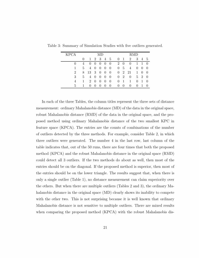
Table 3: Summary of Simulation Studies with five outliers generated.

KPCA MD RMD0 1 2 3 4 5 0 1 2 3 4 5

0 4 0 0 0 0 0 2 0 0 1 1 01 5 4 0 0 0 0 0 5 4 0 0 02 8 13 3 0 0 0 0 2 21 1 0 03 5 4 0 0 0 0 0 2 0 5 2 04 1 2 0 0 0 0 0 1 1 0 1 05 1 0 0 0 0 0 0 0 0 0 1 0

In each of the three Tables, the column titles represent the three sets of distance

measurement: ordinary Mahalanobis distance (MD) of the data in the original space,

robust Mahalanobis distance (RMD) of the data in the original space, and the pro-

posed method using ordinary Mahalanobis distance of the two smallest KPC in

feature space (KPCA). The entries are the counts of combinations of the number

of outliers detected by the three methods. For example, consider Table 2, in which

three outliers were generated. The number 4 in the last row, last column of the

table indicates that, out of the 50 runs, there are four times that both the proposed

method (KPCA) and the robust Mahalanobis distance in the original space (RMD)

could detect all 3 outliers. If the two methods do about as well, then most of the

entries should be on the diagonal. If the proposed method is superior, then most of

the entries should be on the lower triangle. The results suggest that, when there is

only a single outlier (Table 1), no distance measurement can claim superiority over

the others. But when there are multiple outliers (Tables 2 and 3), the ordinary Ma-

halanobis distance in the original space (MD) clearly shows its inability to compete

with the other two. This is not surprising because it is well known that ordinary

Mahalanobis distance is not sensitive to multiple outliers. There are mixed results

when comparing the proposed method (KPCA) with the robust Mahalanobis dis-

21

tance in the original space (RMD) where each method wins over the other in some

cases.

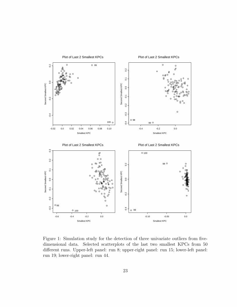
Figures 1 and 2 show scatterplots of the last two smallest KPCs in examples

where the robust Mahalanobis distance in the original space detects more of the

outliers than the proposed method. For example, the lower-right panel of Figure

1 is a scatterplot from run 44 where three outliers were generated. By applying

the methods described above, all three outliers are identified by using the robust

Mahalanobis distance in the original space (RMD), but only two out of the three

outliers are identified by using the ordinary Mahalanobis distance calculated on

the last two smallest KPCs (KPCA). However, the plot clearly suggests that all

three outliers stand out from the majority of the data points. If we calculate the

robust Mahalanobis distance on the last two smallest KPCs, then the remaining

outlier can be identified as well. This is true for all instances where the robust

Mahalanobis distance wins over the proposed method. From these simulations, we

are confident that the proposed method performs as well as the robust Mahalanobis

distance in the original space, which is the best method currently available for

detecting univariate outliers. Although the simulation model assumes the outliers

have larger variance than the regular points, all of them share the same mean from a

multivariate normal distribution. Therefore, the conclusion made is only applicable

to this specific model. Further research will explore models where difference in

location or difference in distributions will be considered.

4.2 Hawkins–Bradu–Kass Data

This example uses a dataset specially constructed by Hawkins, Bradu, and Kass

(1984), which consists of 75 points in 3 dimensions plus a response. In our applica-

tion, we only study the three predictor variables. We refer to this dataset as HBK.

The first 14 points were designed to be outliers. Hawkins et al. show that by using

22

Smallest KPC

Sec

ond

Sm

alle

st K

PC

-0.02 0.0 0.02 0.04 0.06 0.08 0.10

-0.4

-0.2

0.0

0.2

Plot of Last 2 Smallest KPCs

99

100

Smallest KPC

Sec

ond

Sm

alle

st K

PC

-0.4 -0.2 0.0-0

.4-0

.3-0

.2-0

.10.

00.

10.

2

Plot of Last 2 Smallest KPCs

9899

Smallest KPC

Sec

ond

Sm

alle

st K

PC

-0.6 -0.4 -0.2 0.0

-0.3

-0.2

-0.1

0.0

0.1

0.2

0.3

Plot of Last 2 Smallest KPCs

100

99

Smallest KPC

Sec

ond

Sm

alle

st K

PC

-0.10 -0.05 0.0

-0.4

-0.2

0.0

0.2

Plot of Last 2 Smallest KPCs

100

98

99

Figure 1: Simulation study for the detection of three univariate outliers from five-dimensional data. Selected scatterplots of the last two smallest KPCs from 50different runs. Upper-left panel: run 8; upper-right panel: run 15; lower-left panel:run 19; lower-right panel: run 44.

23

Smallest KPC

Sec

ond

Sm

alle

st K

PC

-0.15 -0.10 -0.05 0.0 0.05

-0.1

0-0

.05

0.0

0.05

0.10

Plot of Last 2 Smallest KPCs

100

97

Smallest KPC

Sec

ond

Sm

alle

st K

PC

0.0 0.02 0.04 0.06 0.08-0

.2-0

.10.

00.

10.

2

Plot of Last 2 Smallest KPCs

100

96

99

97

Smallest KPC

Sec

ond

Sm

alle

st K

PC

-0.1 0.0 0.1 0.2 0.3 0.4

-0.2

0.0

0.2

0.4

Plot of Last 2 Smallest KPCs

100

96

97

98

Smallest KPC

Sec

ond

Sm

alle

st K

PC

-0.4 -0.3 -0.2 -0.1 0.0 0.1

-0.1

5-0

.10

-0.0

50.

00.

050.

100.

15

Plot of Last 2 Smallest KPCs

96

98

97

100

99

Figure 2: Simulation study for the detection of five univariate outliers from five-dimensional data. Selected scatterplots of the last two smallest KPCs from 50different runs. Upper-left panel: run 8; upper-right panel: run 15; lower-left panel:run 22; lower-right panel: run 29.

24

Observation

Ma

ha

lan

ob

is D

ista

nce

0 20 40 60

01

02

03

04

0 14

First Smallest KPCS

eco

nd

Sm

alle

st

KP

C

-0.10 -0.05 0.0 0.05

-0.0

50

.00

.05

0.1

0

1,13

11,12,14

5,8 10942367

Figure 3: HBK Data. Left panel: Scatterplot of Mahalanobis distance suggestsonly one outlier could be detected; Right panel: Scatterplot of the last two smallestKPCs suggests all outliers could be detected

an unweighted median and a weighted median, they can separate the 14 outliers into

10 high-leverage outliers and four high-leverage inliers. Rocke and Woodruff (1996)

also identify these 14 particular outliers. If we use ordinary Mahalanobis distance,

only point 14 is detected, as seen in the top panel of Figure 3. In this application,

the other 13 points are said to be “masked” by the 14th point (Hawkins, 2006).

Performing KPCA using RBF kernel with σ = 1, we find six “large” eigenvalues

and 69 “small” eigenvalues. The threshold C is estimated to be 0.0026, so that we

ignore all the KPCs that explain less than 0.26% of the total variance. Therefore,

the 15th KPC is chosen as the smallest KPC. When we plot the smallest KPC

against the second smallest KPC, as shown in the bottom panel of Figure 3, we

see that the first 14 points are perpendicular to the remaining points. The KPCA

scores of the smallest KPC, given in Table 4, show that the magnitudes of the first

14 points are, on average, 1000 times that of the remaining points. Therefore, we

25

Table 4: HBK data. Scores of the smallest KPCs.

(1) 5 × 10−3 4 × 10−2 −7× 10−2 7 × 10−2 −1 × 10−2 −8× 10−2 −1 × 10−1

(8) −1 × 10−2 7 × 10−2 9 × 10−2 −1 × 10−3 −5 × 10−3 5 × 10−3 −2 × 10−3

(15) 3 × 10−6 8 × 10−6 1 × 10−5 −5 × 10−6 −5 × 10−6 1 × 10−5 6 × 10−6

(22) −5 × 10−6 −3× 10−6 −5× 10−6 7 × 10−6 −4 × 10−6 −3× 10−6 −6 × 10−6

(29) −2 × 10−6 −6× 10−6 1 × 10−6 6 × 10−6 −5 × 10−6 2 × 10−5 8 × 10−6

(36) −3 × 10−6 2 × 10−6 −3× 10−6 −3 × 10−7 5 × 10−6 3 × 10−6 7 × 10−6

(43) −3 × 10−6 −6× 10−6 1 × 10−6 −7 × 10−6 −3 × 10−7 2 × 10−6 2 × 10−5

(50) −8 × 10−6 −3× 10−7 −1× 10−7 −5 × 10−6 −5 × 10−6 5 × 10−7 −5 × 10−6

(57) −3 × 10−6 −4× 10−6 −9× 10−6 5 × 10−6 −5 × 10−6 1 × 10−6 −2 × 10−7

(64) −5 × 10−6 −6× 10−6 1 × 10−5 −2 × 10−6 5 × 10−6 −1× 10−6 −9 × 10−6

(71) −5 × 10−6 4 × 10−7 −3× 10−6 1 × 10−5 4 × 10−7

conclude that the these points are outliers.

4.3 Real-Data Examples

This section illustrates the methodology of this paper — by which we use the

smallest KPCs method for finding outliers in feature space — to two well-known

datasets. Only the RBF kernel is applied with different values of the scale parameter

σ in order to reach the best solution.

4.3.1 Bushfire Data

These data were used by Campbell (1989) to locate bushfire scars. The data consist

of satellite measurements at p = 5 frequency bands, corresponding to each of n = 38

pixels. Maronna and Yohai (1995) analyzed the data and concluded that there were

two groups of outliers: points 7–11 and points 32–38. The data were also studied by

Rocke and Woodruff (1996), who found points 8, 9, 32–38 to be extreme outliers and

points 7, 10, 11, and 31 to be less extreme outliers. Performing KPCA using a RBF

kernel with σ = 8, we found two “large” eigenvalues and 36 “small” eigenvalues.

26

First Smallest KPC

Second S

malle

st K

PC

-0.1 0.0 0.1 0.2

-0.4

-0.2

0.0

0.2

0.4

0.6

32

981011

7

33-38

Figure 4: The Bushfire data. Scatterplot of the smallest KPC vs. the second smallestKPC show that there are two groups of outliers, points 32–38 (top) and 7–11 (lowerright).

Figure 4 displays a scatterplot of the smallest and the second smallest KPCs, where

we confirm the division into two groups of outliers, namely, 32–38 (top of Figure 4)

and 7–11 (lower right in Figure 4).

4.3.2 Education Expenditure Data

These data were used by Chatterjee, Hadi, and Price (2000) as an example of het-

eroscedasticity. The data give the education expenditures for the 50 U.S. States

as projected in 1975. The data were also studied by Rousseeuw and Leroy (1987,

pp. 109–112). There are three explanatory variables, X1 (number of residents per

thousand residing in urban areas in 1970), X2 (per capita personal income in 1973),

X3 (number of residents per thousand under 18 years of age in 1974), and one re-

27

First Smallest KPC

Second S

malle

st K

PC

-0.10 -0.05 0.0 0.05

-0.1

0.0

0.1

0.2

50

Figure 5: The Education Expenditure data. Scatterplot of smallest KPC vs. thesecond smallest KPC shows that the fiftieth data point is an outlier.

sponse variable Y (per capita expenditure on public education in 1975). Chatterjee

and Price analyzed these data by using weighted least-squares regression. They con-

sidered the fiftieth case (Hawaii) as an outlier and decided to omit it. Rousseeuw

and Leroy also identified Hawaii as an outlier by analyzing the residual plot from

a least median-of-squares regression. Performing KPCA using a RBF kernel with

σ = 4, we found four “large” eigenvalues and 46 “small” eigenvalues. A scatterplot

of the smallest and the second smallest KPC is displayed in Figure 5; we see that

the fiftieth case is clearly identified as an outlier.

5. CONCLUDING REMARKS

In this article, we investigate a new method for outlier detection using the small-

est kernel principal components (KPCs). We show that the eigenvectors correspond-

28

ing to the smallest KPCs can be viewed as those for which the residual sum of squares

is minimized, so that we could use those components to detect outliers with simple

graphical techniques. The threshold between “large” and “small” eigenvalues is de-

termined, and a method to determine the smallest KPC is suggested. Simulation

studies show that in the univariate outlier situation, the proposed method performs

as well as the best method available. The given examples show that this method is

at least as useful as other methods, and sometimes is better. Possible directions for

future research include fine-tuning the method we propose here, especially the way

the smallest KPC is determined.

References

[1] Campbell, N.A. (1989), “Bushfire Mapping Using NOAA AVHRR Data”, Tech-

nical Report, CSIRO.

[2] Chatterjee, S., Hadi, A.S., and Price, B. (2000), Regression Analysis by Exam-

ple, Third Edition, New York: John Wiley.

[3] Donnell, D.J., Buja, A. and Stuetzle, W. (1994) “Analysis of Additive Depen-

dencies and Concurvities Using Smallest Additive Principal Components”, The

Annals of Statistics, 22, 1635–1673.

[4] Gnanadesikan, R. (1977), Methods for Statistical Analysis of Multivariate Ob-

servations, New York: John Wiley.

[5] Gnanadesikan, R. and Kettenring, J.R. (1972), “Robust Estimates, Residuals,

and Outlier Detection With Multivariate Data,” Biometrics, 28, 81–124.

[6] Gnanadesikan, R. and Wilk, M.B. (1966), “Data Analytic Methods in Mul-

tivariate Statistical Analysis.” General Methodology Lecture on Multivariate

29

Analysis, 126th Annual Meeting, American Statistical Association, Los Ange-

les.

[7] Gnanadesikan, R. and Wilk, M.B. (1969), “Data Analytic Methods in Mul-

tivariate Statistical Analysis,” In: Multivariate Analysis II (P.R. Krishnaiah,

ed.), New York: Academic Press, pp. 593–638.

[8] Gohberg, I., Goldberg, S. and Kaashoek, M.A. (2003), “Basic Classes of Linear

Operators,” Birkhauser.

[9] Hawkins, D.M. (2006), “Masking and Swamping,” Encyclopedia of Statistical

Sciences, New York: Wiley.

[10] Hawkins, D.W., Bradu, D., and Kass, G.V. (1984), “Location of Several Out-

liers in Multiple Regression Data Using Elemental Sets,” Technometrics, 26,

197–208.

[11] Hotelling, H. (1933), “Analysis of a Complex of Statistical Variables with Prin-

cipal Components,” Journal of Educational Psychology, 24, 498–520.

[12] Izenman, A.J. (2008), Modern Multivariate Statistical Techniques: Regression,

Classification, and Manifold Learning, New York: Springer.

[13] Jorgens, K. (1982), “Linear Integral Operators,” Pitman Advanced Publ. Pro-

gram, Boston– London–Melbourne.

[14] Maronna, R.A. and Yohai, V.J. (1995), “The Behavior of the Stahel–Donoho

Robust Multivariate Estimator,” Journal of the American Statistical Associa-

tion, 90, 330–341.

[15] McDiarmid, C. (1989), “On the Method of Bounded Differences,” Surveys in

Combinatorics, Cambridge University Press, 148–188.

30

[16] Mercer, J. (1909), “Functions of Positive and Negative Type and Their Con-

nection with the Theory of Integral Equations,” Philosophical Transactions of

the Royal Society, London.

[17] Rocke, D.M. and Woodruff, D.L. (1996), “Identification of Outliers in Multi-

variate Data,” Journal of the American Statistical Association, 91, 1047–1061.

[18] Rousseeuw, P.J. and Leroy, A.M. (1987), Robust Regression and Outlier Detec-

tion, New York: John Wiley.

[19] Scholkopf, B. and Smola, A.J. (2002), Learning with Kernels, Cambridge, MA:

MIT Press.

[20] Scholkopf, B., Smola, A.J., and Muller, K.-R. (1998), “Nonlinear Component

Analysis as a Kernel Eigenvalue Problem,” Neural Computation, 10, 1299–1319.

[21] Scholkopf, B., Mika, S., Burges, C., Knirsch, P., Muller, K., Ratsch, G., and

Smola, A. (1999), “Input Space Versus Feature Space in Kernel-Based Meth-

ods,” IEEE Transactions on Neural Networks, 10(5), 1000–1017.

[22] Shawe-Taylor, J. and Cristianini, N. (2004), Kernel Methods for Pattern Anal-

ysis, Cambridge, U.K.: Cambridge University Press.

[23] Shen, Y. (2007), Outlier Detection Using the Smallest Kernel Principal Com-

ponents, Ph.D. dissertation, Department of Statistics, Temple University.

[24] Tukey, J.W. (1977), Exploratory Data Analysis. Reading, MA: Addison-Wesley.

31