Outlier Detection in Urban Air Quality Sensor Networks

V. M. van Zoest & A. Stein & G. Hoek

Received: 16 October 2017 /Accepted: 21 February 2018 /Published online: 8 March 2018# The Author(s) 2018. This article is an open access publication

Abstract Low-cost urban air quality sensor networksare increasingly used to study the spatio-temporal vari-ability in air pollutant concentrations. Recently installedlow-cost urban sensors, however, are more prone toresult in erroneous data than conventional monitors,e.g., leading to outliers. Commonly applied outlier de-tection methods are unsuitable for air pollutant measure-ments that have large spatial and temporal variations asoccur in urban areas. We present a novel outlier detec-tion method based upon a spatio-temporal classification,focusing on hourly NO2 concentrations.We divide a fullyear’s observations into 16 spatio-temporal classes,reflecting urban background vs. urban traffic stations,weekdays vs. weekends, and four periods per day. Foreach spatio-temporal class, we detect outliers using themean and standard deviation of the normal distributionunderlying the truncated normal distribution of the NO2

observations. Applying this method to a low-cost airquality sensor network in the city of Eindhoven, theNetherlands, we found 0.1–0.5% of outliers. Outliers

could reflect measurement errors or unusual high airpollution events. Additional evaluation using expertknowledge is needed to decide on treatment of theidentified outliers. We conclude that our method is ableto detect outliers while maintaining the spatio-temporalvariability of air pollutant concentrations in urban areas.

Keywords Airquality .Air pollution .Outlier detection .

NO2. Sensor network

1 Introduction

Air quality is monitored globally, with national monitor-ing networks being used to assess air pollution in relationto environmental limit values. In Europe, national, re-gional, and local environmental agencies operate thesemonitoring networks according to EU guidelines(European Parliament and Council of the EuropeanUnion 2008), complying to high standards of equivalen-cy (EC Working Group on GDE 2010). Each Europeancountry has a network of air quality monitoring stationsthat are located in urban, suburban, and rural areas.

Health effects of air pollution have attracted publicand scientific attention globally as the global burden ofdisease of outdoor air pollution is significant (Cohenet al. 2017). The health risks are typically highest inurban areas because of their high population density, ahigh density of schools and hospitals, and higher airpollution concentrations. In recent local networks, urbanair quality is measured using a larger number of sensorsthan in national air quality networks, allowing detection

Water Air Soil Pollut (2018) 229: 111https://doi.org/10.1007/s11270-018-3756-7

Electronic supplementary material The online version of thisarticle (https://doi.org/10.1007/s11270-018-3756-7) containssupplementary material, which is available to authorized users.

V. M. van Zoest (*) :A. SteinFaculty of Geo-Information Science and Earth Observation (ITC),University of Twente, PO Box 217, 7500 AE Enschede,The Netherlandse-mail: v.m.vanzoest@utwente.nl

G. HoekInstitute for Risk Assessment Sciences (IRAS), UtrechtUniversity, PO Box 80178, 3508 TDUtrecht, The Netherlands

of more local sources. In response to the increasing civilinterest in the air they breathe, more local initiativeshave resulted in extended low-cost monitoring net-works. These provide more detailed spatio-temporaldata on air quality. Data from such sensor networkshowever are more prone to result in errors, and theirspatio-temporal data quality is often unknown (Snyderet al. 2013). This leads to an increased need for dataevaluation. Data evaluation of low-cost air quality net-works typically includes outlier detection, comparisonwith classical monitors, comparison of inter-sensor mea-surements, and evaluation of the stability of sensors. Inthis paper, we focus on outlier detection.

Outlier detection is an important part of data cleaningand particularly relevant for low-cost air quality sensornetworks. Outlier detection is defined as the detection ofvalues that are statistically significantly different fromthe expected value at a given time and location. Outlierdetection is important not only for detecting air pollutionevents but also for removing errors that might otherwiseaffect data analysis and comparison, including unneces-sary unrest among the population if data are publiclyavailable online. Errors in this context refer to inaccura-cies due to air quality sensor faults, mistakes in thehuman handling of the sensors, or positioning of thesensors under conditions for which they are not de-signed. Events are valid observations of very high orlow air pollutant concentrations compared to the con-centrations expected at a given time in a given location(Zhang et al. 2007). True events can be related to verylocal sources (e.g., a small fire, truck idling withinmeters of a monitor) or to very unusual weather circum-stances such as low mixing height and high atmosphericstability resulting in poor dispersion of emittedpollutants.

Functional outlier detection, as a common type oftemporal outlier detection, compares various functioncurves of fixed time periods. In the past, this methodwas applied to PM10, SO2, NO, NO2, CO, and O3 todetect months with unusually high air pollutant concen-trations (Martínez Torres et al. 2011), or to detect work-ing days and non-working days with outlying NOx

levels (Febrero et al. 2007, 2008; Sguera et al. 2016).Functional outlier detection is used to compare entirevectors of measurements (e.g., all observations in amonth) and is therefore less suitable for the detectionof individual outliers. Comparing an observation only toits temporal neighborhood may also lead to the neglectof a systematic bias in the sensor.

In spatial outlier detection, an observation is com-pared to the observations in its spatial neighborhood.Bobbia et al. (2015) used kriging to detect outliers inPM10 concentrations on a provincial scale. Spatio-temporal outlier detection combines the spatial neigh-borhood with a temporal neighborhood. It has beenapplied to PM10 measurements at the European scale(Kracht et al. 2014). At this scale level, however, onlyrural and urban background stations can be used, as themethods are not suitable for dealing with the widespatial variation of air pollutants in an urban area.

For an urban air quality sensor network, both spatialand spatio-temporal outlier detection have only beenapplied to air pollutants that show a low spatial varia-tion. Hamm (2016) and Shamsipour et al. (2014) ap-plied spatial and spatio-temporal outlier detectionmethods on PM10, which in cities is mostly dominatedby regional background concentrations from sourcesoutside the city (Eeftens 2012). Distance-weightingtechniques such as kriging were successfully appliedto urban PM10 for filling missing values and for outlierdetection. There was no need for space varying covari-ates because PM10 concentration was not related to thetype of location or street (Hamm 2016). For NO2, how-ever, the concentrations can vary over short distances,e.g., governed by the traffic density of a street (Briggs1997; Cyrys 2012). As the distances over which NO2

concentrations vary (tens of meters) are commonlyshorter than the distances between sensor locations (ki-lometers), spatial outlier detection methods based ondistance-weighting cannot be applied to NO2 measure-ments in cities.

The objective of this study was to develop an adequateoutlier detection method for an urban air quality sensornetwork. Such a network is characterized by a fine-scalespatial and temporal variation in air quality. For this study,we use NO2 data from an air quality sensor networklocated in the city of Eindhoven, the Netherlands.

2 Data Preprocessing

The air quality sensor network in Eindhoven (Fig. 1)was established by the AiREAS civil initiative (Close2016), and is the first fine resolution urban air qualitysensor network in the Netherlands. It was installed inNovember 2013 and has been operated continuouslysince. The network consists of 35 weatherproof airboxesof size 43 × 33 × 20 cm, containing an array of sensors.

111 Page 2 of 13 Water Air Soil Pollut (2018) 229: 111

Each airbox measures particulate matter, ozone (O3),and/or nitrogen dioxide (NO2) and also temperatureand humidity as the air flows through (Hamm et al.2016). The airboxes have a fixed position and are at-tached to lamp posts for power supply.

We focus on NO2, as an air pollutant with a highspatial variability in urban areas (Cyrys 2012). The hour-ly concentrations measured by the conventional moni-tors in Eindhoven ranged from 2.5 to 123.8 μg m−3 in2016, with a mean of 28.6 μg m−3 and a standarddeviation of 16.5 μg m−3. The distribution of NO2 con-centrations is skewed with a long right tail (P95 =61.0 μg m−3, P99 = 78.8 μg m

−3). The airboxes measureNO2 concentrations using a Citytech Sensoric NO2 3E50sensor adapted by the Energy Research Center of theNetherlands (ECN). The concentration of air pollutantsis measured every 10 min. The data are sent to a serverusing a GPRS connection (Hamm et al. 2016). To reducethe noise, the 10-min NO2 measurements were averagedto hourly values for the current analysis. Data for the full

year of 2016 were used for this study. The sensors werecalibrated at the end of 2015.

The data were cleansed before being used. Negativeconcentration values occurred when the concentrationswere below the limit of detection and were removed fromthe dataset (1.5%). Zeroes in the data indicated a sensorfailure and were removed from the dataset (1%). Highpeaks in NO2 concentrations can occur in 10-min data ifthe sensor is exposed to a high concentration peak for ashort period of time. Similar peaks in hourly concentrationdata however aremore likely to be caused by sensor failureand influence the outlier detection. To carefully removeextreme peaks in hourly concentrations, we turned to thetwo conventional NO2 monitors in Eindhoven, which arepart of the national air quality monitoring network. We seta threshold equal to three times the maximum hourlyconcentration measured in 2016. In doing so, concentra-tion values xi> 372 μg m

−3 were removed (0.02%). Suchextreme peaks are impossible to occur under natural con-ditions in this city and are most probably caused by sensor

Fig. 1 Locations of the airboxes in the city of Eindhoven, the Netherlands, at urban background locations (circles) and urban trafficlocations (triangles)

Water Air Soil Pollut (2018) 229: 111 Page 3 of 13 111

failures. Such failures also caused frozen concentrationvalues for several hours or days. Those values were re-moved from the dataset as well (1.5%). One airboxshowed a consistent positive bias. Including it in theanalysis not only showed the many outliers of the airboxbut also strongly influenced the percentage of outliers thatcould be detected in other airboxes, which almost droppedto zero. Therefore, data of this airbox was removed prior tothe final outlier detection shown here.

3 Methods

Outlier detection is based upon checking whether anobserved concentration value falls within a given confi-dence interval, set by

μ� z� σ ð1Þwhere μ is the mean NO2 concentration level in μg m

−3,σ is the standard deviation, and z is an indicator of thesize of the confidence interval. We consider Eq. (1) forgrouped NO2 concentration observations within tempo-ral, spatial, and spatio-temporal neighborhoods. Assum-ing independence and normality, then the value of z is setat 1.96 for a 95% confidence level (Kracht et al. 2014) orat 2.97 for a 99.7% confidence interval, depending on therequired strictness of the outlier detection. We used z =2.97, which in related studies has been rounded to z = 3(Martínez Torres et al. 2011; Shamsipour et al. 2014).

NO2 concentrations in an urban setting, however,highly depend on the proximity of busy roads, andtherefore, too much noise in concentrations is foundwithin the neighborhood to detect values that are abnor-mally high given their location. Similarly, temporalneighborhoods have a highly temporally dependent var-iation in air pollutant concentrations over the day.

We propose to overcome this by classifying the lo-cations and time periods into 16 spatio-temporal cate-gories distinguished by different levels of air pollution.To do so, we divided the measurement locations intotwo categories: urban traffic and urban backgroundlocations. These take into account the positions of theairboxes near specific land use types, the presence oftraffic, and distance from the center. We take four inter-vals: traffic hours (6:01–9:00 and 16:01–20:00 UTCtime), off-peak hours (9:01–16:00 and 20:01–22:00UTC time), transition periods (22:01–1:00 and 5:01–6:00UTC time), and night hours (1:01–5:00UTC time).

Days of the week were divided into two classes:weekdays (Monday to Friday) and weekend days (Sat-urday and Sunday). This all resulted into 16 classes:eight temporal classes and two spatial classes. For eachspatio-temporal class K, the three steps described beloware taken to detect outliers.

1. We transformed the NO2 concentrations using thesquare root transformation to obtain approximatelynormally distributed values (Fig. 2), i.e., to justifythe use of Eq. (1).

Before transforming the NO2 concentration values, inline with Kracht et al. (2013), we added a value of (1 −minimum value of all observations) to all observations toprevent values < 1 μg m−3 from increasing during squareroot transformation while values > 1 μg m−3 decrease:

xc ¼ffiffiffiffiffiffiffiffiffiffiffiffiffiffiffiffiffiffiffiffiffiffiffiffiffiffiffiffiffiffiffiffiffiffiffiffiffiffiffiffiffiffiffiffiffiffiffiffiNO2c þ 1−min NO2cð Þð Þ

pð2Þ

where NO2c is an observation and xc is the transformedobservation in spatio-temporal class K, where K ¼ ⋃c∈Cxcð Þ and c is an observation index in C = {1…NC} for NC

total number of observations in class K. Note that xc hascoordinates in space and time.

2. As a result of the transformation in Eq. (2), thedistribution of NO2 concentrations is truncated atthe left at 1 μg m−3. The resulting distribution thusshowed a truncated normal distribution (Fig. 3).

For each square-root-transformed NO2 observationxc, i, we temporarily excluded the ith observation fromthe NO2 concentration dataset in order to avoid impactof the observation, a potential outlier, on the standarddeviation and mean. We then obtained the mean andstandard deviation of the remainder of the dataset as

m−iK ¼ ∑c xcð Þ−xc;i

NC−1ð Þ ð3Þ

s−iK ¼ffiffiffiffiffiffiffiffiffiffiffiffiffiffiffiffiffiffiffiffiffiffiffiffiffiffiffiffiffiffiffiffiffiffiffiffiffiffiffiffiffiffiffiffiffiffiffiffiffi∑c xc−m−i

K

� �2− xc;i−m−iK

� �2NC−2ð Þ

sð4Þ

where summation extends over all hourly NO2 observa-tions xc in one spatio-temporal class K and m−i

K and s−iKare the mean and the standard deviation of all hourly

111 Page 4 of 13 Water Air Soil Pollut (2018) 229: 111

NO2 observations excluding the ith observation xc, i,respectively. Note that c, i ∈C and NC is the total num-ber of observations in class K.

Equations (3) and (4) provided both the mean and thestandard deviation of the truncated normal distributionof NO2 concentrations, referred to as m−i

K and s−iK . Equa-tion (1) requires a normal distribution, and therefore, weare more interested in the mean and standard deviationof the underlying normal distribution, referred to n−iK andt−iK , respectively, rather than the mean and standarddeviation of the truncated normal distribution. We usea maximum likelihood estimator to obtain estimatedvalues n−iK and t−iK . The log likelihood function is givenas

∑cln f xcjθð Þð Þ ð5Þ

where f(xc| θ) is the probability density function of thetruncated normal distribution of NO2 concentrations,returning the probability of observing xc given a set ofparameters θ ¼ m−i

K ; s−iK ; a; b

� �, for a ≤ x ≤ b. In our case

of left truncation, we have a = 1 and b =∞. Then, theprobability density function is given as

f xcjθð Þ ¼ϕ

xc−n−iKt−iK

� �

t−iK 1−Φa−n−iKt−iK

� �� � ð6Þ

Imputing Eq. (6) into the log likelihood function andtaking θ1 ¼ n−iK ; t

−iK

� �gives

L θ1ð Þ ¼ ∑c ln ϕxc−n−iKt−iK

� �� �−ln t−iK 1−Φ

a−n−iKt−iK

� �� �� �� �ð7Þ

where ϕ(∙) is the probability density function of thenormal distribution and Φ(∙) is the corresponding cumu-lative distribution function. Optimization of the loglikelihood function Eq. (7) using Nelder and Mead(1965) gives maximum likelihood values for n−iK andt−iK . We used the parameters m−i

K and s−iK as startingvalues.

For each observation xc, i removed from the dataset,n−iK and t−iK are computed on the remainder of thespatio-temporal class dataset as described above.

3. Next, Eq. (1) is adapted to find the lower and upperthresholds of values considered outliers:

n−iK � z� t−iK ð8Þ

which is computed for each individual observation. Ifthe ith observation xc, i falls outside this interval, it isconsidered to be an outlier. The observations of spatio-temporal class K are backtransformed after the outlierdetection:

NO2c ¼ xcð Þ2− 1−min xcð Þð Þ ð9Þreturning the NO2 concentrations in μg m−3. Dependingupon the purpose of the outlier detection, the outlyingobservations can then be removed or further investigated.

We further computed the thresholds for the entiredataset, without removal of observation xc, i in Eqs. (3)and (4). The mean and standard deviation of the under-lying normal distribution are then expressed by nK and tK,respectively, which results in the following thresholds:

nK � z� tK ð10Þwhich are also back-transformed using Eq. (9). Thesethresholds are not used for actual outlier detection, butas an approximation of the thresholds for each spatio-temporal class. This allowed us to compare the thresholdsof the 16 spatio-temporal classes. Given the large numberof observations in each class, the thresholds are not highlyaffected by removing one of the observations.

For comparison with conventional monitors, thesame analysis was repeated with data from the twoNO2 monitors in Eindhoven which are part of the na-tional air quality monitoring network. Both convention-al monitors are located in an urban traffic location andtherefore considered as the same spatial class. We usedthe temporal classification similar to the one used in theanalysis of the airbox data.

4 Results

Of the 25 airboxes measuring NO2 that were used forthis analysis, 11 were classified as urban backgroundlocations, and 14 were classified as urban traffic loca-tions. Table 1 shows the approximated upper thresholdsfor outliers in each spatio-temporal class (Eq. (10)). Alllower thresholds were equal to zero. For the values of ncand tc of each spatio-temporal class, we refer to Table S1

Water Air Soil Pollut (2018) 229: 111 Page 5 of 13 111

in the supplementary materials. Table 2 shows the per-centage of outliers detected per spatio-temporal NO2

concentration class using a full year of hourly NO2 data.Note that our method defines unusual observations,which are not necessarily errors, but which could alsobe very unusual air pollution events related to localsources, or extreme weather conditions of low windspeed and high atmospheric stability.

Table 2 shows that the period of night hours during theweekend has an increase in the number of outliers, bothfor urban traffic locations and urban background loca-tions. Both nc and tc are relatively small in these spatio-temporal classes compared to other spatio-temporal clas-ses. The combination of a short right tail and the relativelysmall nc and tc cause the upper threshold to be low whiledetecting a relatively high number of outliers in thethicker tail. All categories have an approximately similarpercentage of outliers and there are no large deviations.

The boxplots in Fig. 4 show the range in concentrationsthat were considered outliers for each spatio-temporalclass. The lower whiskers are short and close to thethreshold values shown in Table 1. Especially duringoff-peak hours in theweekend, the range in concentrationsof the outliers is large. Extreme outliers, denoted by thedots, representing observations outside 1.5 × IQR (inter-quartile range) of the outliers, occur in many spatio-temporal classes. Note that these boxplots are only basedon the outliers, which is a small number of observations.

Figures 5 and 6 show NO2 measurements during2 weeks in 2016 containing outliers. Figure 5 shows theweek from April 25 until May 1, of an urban backgroundlocation, whereas Fig. 6 shows the week from February 8until February 14 of an urban traffic location. The con-centrations at the urban traffic location were higher thanthose at the urban background location. Due to the spatial

NO2 concentration (µg/m3)0 100 200 300 400

020

000

4000

060

000

8000

010

0000

a

NO2 concentration (µg/m3)0 5 10 15 20 25

010

000

2000

030

000

4000

050

000b

Freq

uenc

yFr

eque

ncy

Fig. 2 Distribution of NO2 concentrations a before square roottransformation and b after square root transformation

0−5

0.00

0.05

0.10

0.15

0.20

0.25

0.30

NO2 concentration (sqrt−transformed)

TruncatedUnderlying Normal Distr.Truncation Point

105 15 20

Den

sity

Fig. 3 The truncated normal distribution of square-root-transformed NO2 concentrations (solid line) and its underlyingnormal distribution (dot dashed line). The truncation point is setat 1 (dotted line)

111 Page 6 of 13 Water Air Soil Pollut (2018) 229: 111

classification, some concentration values are consideredoutliers at the urban background location, while they arenon-outliers at the urban traffic location. The temporalclassification is also visible in Fig. 6: concentration valuesthat are considered outliers at one point in time can beconsidered non-outliers at other points in time, e.g., duringrush hours in which higher concentrations are expected.This is a major difference as compared to applying theoutlier threshold on the entire dataset without classifica-tion (Eq. (1)), yielding an expected 0.3% of outliers ascutoff peaks without taking spatio-temporal variability inthe NO2 concentrations into account.

Figure 5 shows two outliers, labeled (a) and (b),occurring during the night, in the early morning (1:00–3:00) of April 28. During weekday night hours at anurban background location, the transformed (Eq. (2))parameter estimations are nc = 3.965 and tc = 1.265. En-tered in Eq. (8) with z = 2.97, and back transformedusing Eq. (9), this gives an upper threshold of58.6 μg m−3. The concentrations measured at outliers(a) and (b) were 75 and 70.8 μg m−3, respectively, bothexceeding the upper threshold. Given that these areconsecutive observations and within the range of thresh-olds of other periods, it is not clear whether these obser-vations reflect instrument error.

From Fig. 6, we identify four outliers, labeled (a)–(d).Three outliers, specifically (a), (c), and (d), are clearlyhigher than expected concentration values in any of thespatio-temporal categories. They are furthermore singleobservations. Outlier (b) occurred on February 9 from23:00 to 0:00 in the temporal class Btransition period.^In this spatio-temporal class, with (transformed) nc =4.76 and tc = 1.36, the upper threshold is approximately(4.76 + 2.97 × 1.36)2 − (1 − 0.0244) = 76.5 μg m3. Theconcentration measured at (b) is 81.8 μg m−3, exceedingthe upper threshold. However, during the daytime, sucha concentration value would have been within expectedconcentration values.

There was seasonal deviation in the number of out-liers: a higher number of outliers was detected in spring(0.37%) compared to the mean percentage of outliers ofthe entire year (0.22%). In summer, the number ofoutliers was relatively low (0.09%).

Table 2 shows no difference in the percentage ofoutliers between urban traffic locations and urban back-ground locations. Some individual airboxes howevershow more outliers than others. Most airboxes have 0–0.1% outliers for a year of data, whereas a few airboxeshave a larger percentage of outliers for some spatio-temporal classes, up to a maximum of 2.5% for oneairbox for one spatio-temporal class. The highest per-centages of outliers are found in airboxes with thehighest mean concentration values. The percentage ofoutliers of an airbox varies between spatio-temporalclasses.

Similar results were found using hourly NO2 obser-vations of 2016 from the two conventional monitors.The total number of outliers detected was 0.3% of thedataset, which varied from 0 to 0.7% depending on thetemporal class. In Fig. 7, we observe a different patternin the spatio-temporal thresholds compared to thethreshold pattern of the airboxes (Figs. 5 and 6). Note

Table 1 Upper thresholds for hourly average NO2 concentrations (μg m−3) above which considered outliers, per spatio-temporal class,using z = 2.97

Urban traffic Urban background

Week Weekend Week Weekend

Rush hours 96.6 (n = 17,761) 78.4 (n = 7,127) 81.0 (n = 17,660) 62.3 (n = 6,983)

Off-peak hours 87.3 (n = 22,768) 76.7 (n = 9,153) 72.9 (n = 22,554) 61.3 (n = 8,961)

Night hours 63.2 (n = 10,161) 63.6 (n = 4,123) 58.6 (n = 9,983) 57.3 (n = 3,995)

Transition hours 76.5 (n = 10,195) 67.1 (n = 4,129) 67.9 (n = 10,031) 56.4 (n = 3,983)

Between brackets, n shows the number of hourly concentration values in this class

Table 2 Percentage outliers per spatio-temporal NO2 concentra-tion class for hourly values in 2016, using z = 2.97

Urban traffic Urban background

Week Weekend Week Weekend

Rush hours 0.2% 0.2% 0.2% 0.2%

Off-peak hours 0.2% 0.2% 0.2% 0.2%

Night hours 0.2% 0.5% 0.1% 0.5%

Transition hours 0.3% 0.3% 0.3% 0.3%

Water Air Soil Pollut (2018) 229: 111 Page 7 of 13 111

that for the conventional monitors, we also observepositive lower threshold values, though close to zero.In Fig. 7, we identify one outlier, which occurred in theoff-peak hour period after the evening rush hour. Thisperiod after the evening rush hour is the period in whichmost outliers occurred for the conventional monitors.

We compared the outliers in the traffic airboxeswiththe NO2 concentrations measured with the conven-tionalmonitors at the same time.A scatterplot is shownin Fig. 8. The plot shows many observations down-right in the plot that have similarly high concentrationsmeasured by the airbox and the conventional monitor,

though at different locations. Someoutliers occurred inmultiple airboxes at the same time. This may be anindication of a pollution event that has an effect on theentire city. Down-left in the plot, we find observationsthat are considered outliers by the airboxes, but arewithin normal range of concentrations according to theconventional monitors. These could be errors or verylocal air pollution events. In the upper part of the plot,we find very high concentrations measured by theairbox which are higher than any value measured bythe conventional monitor in the entire year. These aremost likely errors.

010

020

030

040

0

NO

2 co

ncen

tratio

ns o

f out

liers

(µg/

m3)

WeekdaysBackground location

WeekdaysTraffic location

Weekend Background location

WeekendTraffic location

Rush hourOff−peakNightTransition

Fig. 4 Boxplots of the outliers in each spatio-temporal class

Apr 25 Apr 27 Apr 29 May 01

010

020

030

040

0

Time (2016)

NO

2 co

ncen

tratio

ns (µ

g/m

3)

Valid observationOutlierSpatio−temporal threshold

a b

Fig. 5 NO2 concentrations measured by airbox 6, an urban background location. Filled circles indicate non-outlying observations; unfilledcircles indicate outliers using z = 2.97. The gray bars indicate the threshold values for each temporal class, for urban background airboxes

111 Page 8 of 13 Water Air Soil Pollut (2018) 229: 111

5 Discussion

The results show that the spatio-temporal classificationof NO2 concentration values in an urban sensor networkis a simple outlier detection method in an area with highspatial and temporal variability of air pollutant concen-trations. The number of outliers detected using the clas-sification (0.1–0.5% for the airboxes and 0–0.7% for theconventional monitors) matches expectation when using

z = 2.97 as a threshold for the number of standard devi-ations, including 99.7% of the observations under theassumption of a normal distribution. The value of z canbe tuned depending on the application. A lower value ofz will result in more concentration values to be consid-ered outliers. Brown and Brown (2012) suggest that thechoice of the threshold value should be a trade-offbetween the extra work associated with investigatingfalse positives, i.e., observations falsely detected as

Feb 09 Feb 11 Feb 13 Feb 15

010

020

030

040

0

Time (2016)

NO

2 co

ncen

tratio

ns (µ

g/m

3)

Valid observationOutlierSpatio−temporal threshold

a

b

c

d

Fig. 6 NO2 concentrations measured by airbox 26, an urban traffic location. Filled circles indicate non-outlying observations; unfilledcircles indicate outliers using z = 2.97. The gray bars indicate the threshold values for each temporal class, for urban traffic airboxes

Feb 15 Feb 17 Feb 19 Feb 21

010

020

030

040

0

Time (2016)

NO

2 co

ncen

tratio

ns (µ

g/m

3)

Valid observationOutlierSpatio−temporal threshold

Fig. 7 NO2 concentrationsmeasured by a conventional monitor atan urban traffic location. Filled circles indicate non-outlying ob-servations; unfilled circles indicate outliers using z = 2.97. The

gray bars indicate the threshold values for each temporal class,for urban traffic conventional monitors

Water Air Soil Pollut (2018) 229: 111 Page 9 of 13 111

outliers, and the likelihood of false negatives, i.e., trueoutliers that are not detected.

We aimed to compare the above procedure withkriging-based outlier detection (Zhang et al. 2012). Wefound that the NO2 concentrations vary over shorterdistances than the distances between measurement loca-tions, resulting in a pure noise variogram. SamplingNO2 over shorter distances, e.g., within a few meters,might make it possible to apply kriging-based outlierdetectionmethods, especially when including covariatessuch as road distance and wind direction into the model.

Air pollutant concentrations are generally consideredlognormally distributed (Ott 1990). Applying the pro-posed outlier detection method on log-transformed NO2

concentrations would however result in an implausiblenumber of outliers detected on the left side on thedistribution (99.5%) compared to the right side of thedistribution (0.5%). Instead, we are mostly interested inhigh peaks in the data, which can be used to detect airpollution events and errors. Therefore, we used a squareroot transformation of the NO2 concentration data.

The temporal classification used in this analysis ismostly based on expected traffic during certain hours ofthe day. Other factors that may influence the temporalvariability in NO2 concentrations are meteorological fac-tors such as wind speed, wind direction, air pressure,temperature, and solar radiation. An analysis of seasonaland diurnal variation at a UK city is presented byBigi and

Harrison (2010). NO2 concentrations in Europe tend to behigher in the winter than in the summer season. Hence,observations in the summer season had a lower chance tobe detected as outliers by our method. Our method can beexpanded by defining more classes, for example, takinginto account season and meteorological factors, or bytaking into account temporal autocorrelation. For simplic-ity reasons, we used full year data for the current paper.

Public holidays occurring on a weekday are classifiedas weekdays, although the concentrations are likelylower, and therefore more similar to weekend concen-trations. A visual analysis of the data showed that therewas no increase in low-peak outliers during such holi-days. High-peak outliers occurred and were also detect-ed during the weekday holidays.

In this study, we aggregated the NO2 concentrationsto hourly values. Using 10-min data, the outlier detectionmethod would give more detailed instances of outlierscompared to using hourly data. The results of 10-minoutlier detection should be interpreted differently fromthe results of hourly outlier detection. In hourly outlierdetection, peaks occurring as a result of a strongly emit-ting vehicle passing by are more likely to be averagedout as they may occur every hour. In 10-min data, suchpeaks are more likely to be considered outliers. Hourlyoutliers give a better overview of hours in which there isan abnormal number of peaks rather than showing indi-vidual peaks, as in the case of 10-min outlier detection.

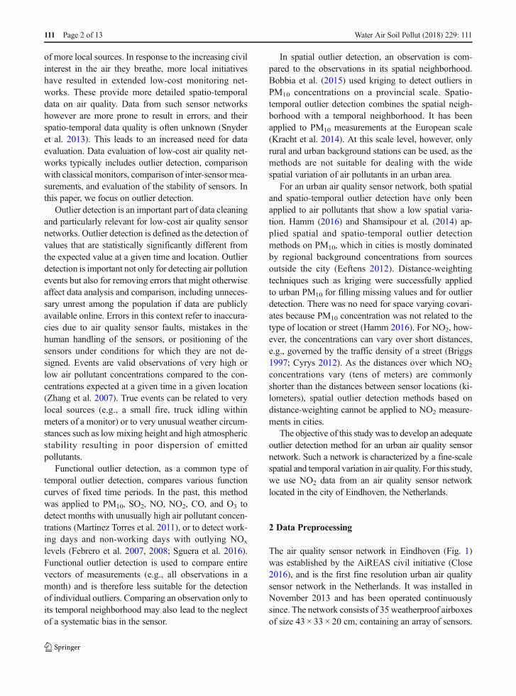
For the conventional monitors, the largest number ofoutliers was found during the off-peak period after theevening rush hours. Comparing the daily threshold pat-tern of the airbox to that of the conventional monitor ona weekday (Fig. 9), both at an urban traffic location, wesee that the upper threshold of the airbox in off-peakperiods (87.3 μg m−3) lays between the upper thresholdof rush hours (96.6 μg m−3) and the upper threshold oftransition periods (76.5 μg m−3). For the conventionalmonitor, the upper threshold for off-peak periods(86.4 μg m−3) is below the threshold for both rush hours(106μgm−3) and transition periods (101.6μgm−3). Thethreshold for off-peak periods is calculated using theobservations between morning rush hour and eveningrush hour (9:01–16:00 UTC time) combined with theobservations after evening rush hour (20:01–22:00 UTCtime). For the airboxes, this is alright because the con-centrations are within a similar range. The authorativemonitors, however, still measure high concentrations for2 h after the evening rush hour. This leads to underesti-mation of the threshold after evening rush hour. The

0 100 200 300 400

010

020

030

040

0

Max. NO2 concentration value (µg/m3) of the two conventional monitors

NO

2 ou

tlier

s (µ

g/m

3) u

rban

traf

fic a

ribox

es

Fig. 8 Scatterplot of traffic airbox outliers vs. the maximum NO2

concentration measured at the same moment in time by the twoconventional monitors located in traffic sites

111 Page 10 of 13 Water Air Soil Pollut (2018) 229: 111

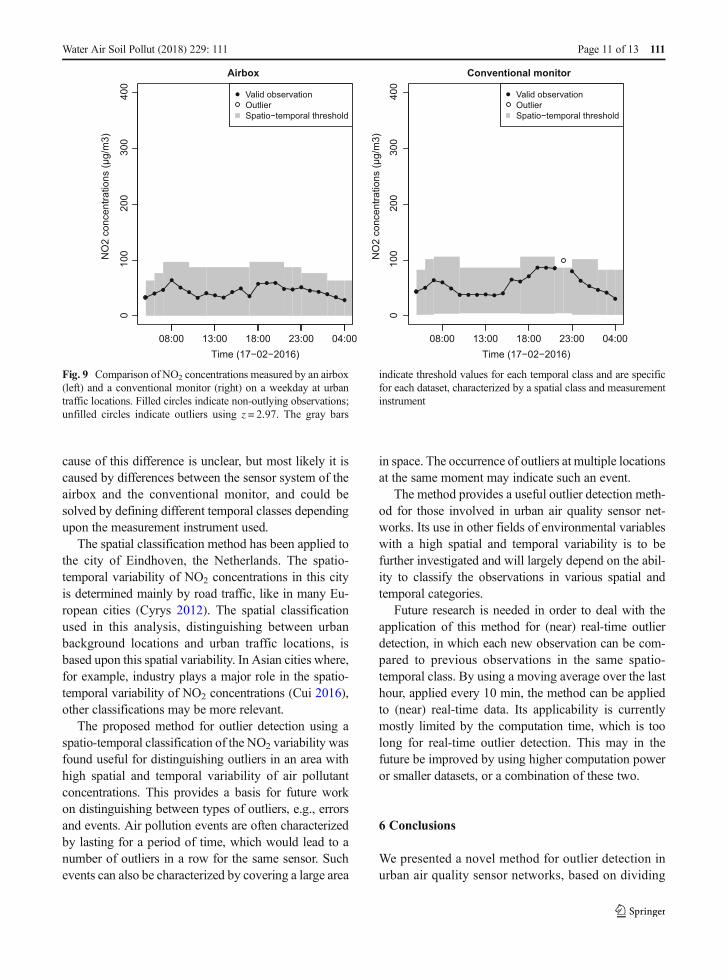
cause of this difference is unclear, but most likely it iscaused by differences between the sensor system of theairbox and the conventional monitor, and could besolved by defining different temporal classes dependingupon the measurement instrument used.

The spatial classification method has been applied tothe city of Eindhoven, the Netherlands. The spatio-temporal variability of NO2 concentrations in this cityis determined mainly by road traffic, like in many Eu-ropean cities (Cyrys 2012). The spatial classificationused in this analysis, distinguishing between urbanbackground locations and urban traffic locations, isbased upon this spatial variability. In Asian cities where,for example, industry plays a major role in the spatio-temporal variability of NO2 concentrations (Cui 2016),other classifications may be more relevant.

The proposed method for outlier detection using aspatio-temporal classification of the NO2 variability wasfound useful for distinguishing outliers in an area withhigh spatial and temporal variability of air pollutantconcentrations. This provides a basis for future workon distinguishing between types of outliers, e.g., errorsand events. Air pollution events are often characterizedby lasting for a period of time, which would lead to anumber of outliers in a row for the same sensor. Suchevents can also be characterized by covering a large area

in space. The occurrence of outliers at multiple locationsat the same moment may indicate such an event.

The method provides a useful outlier detection meth-od for those involved in urban air quality sensor net-works. Its use in other fields of environmental variableswith a high spatial and temporal variability is to befurther investigated and will largely depend on the abil-ity to classify the observations in various spatial andtemporal categories.

Future research is needed in order to deal with theapplication of this method for (near) real-time outlierdetection, in which each new observation can be com-pared to previous observations in the same spatio-temporal class. By using a moving average over the lasthour, applied every 10 min, the method can be appliedto (near) real-time data. Its applicability is currentlymostly limited by the computation time, which is toolong for real-time outlier detection. This may in thefuture be improved by using higher computation poweror smaller datasets, or a combination of these two.

6 Conclusions

We presented a novel method for outlier detection inurban air quality sensor networks, based on dividing

010

020

030

040

0

Airbox

NO

2 co

ncen

tratio

ns (µ

g/m

3)Valid observationOutlierSpatio−temporal threshold

08:00 18:00 04:00

200

010

040

0

Conventional monitor

Time (17−02−2016)

NO

2 co

ncen

tratio

ns (µ

g/m

3)

Valid observationOutlierSpatio−temporal threshold

08:00 18:00 13:00 23:0013:00 23:00 04:00Time (17−02−2016)

300

Fig. 9 Comparison of NO2 concentrations measured by an airbox(left) and a conventional monitor (right) on a weekday at urbantraffic locations. Filled circles indicate non-outlying observations;unfilled circles indicate outliers using z = 2.97. The gray bars

indicate threshold values for each temporal class and are specificfor each dataset, characterized by a spatial class and measurementinstrument

Water Air Soil Pollut (2018) 229: 111 Page 11 of 13 111

the observations in two spatial and eight temporalclasses. Each of the 16 resulting spatio-temporalclasses represents a range of typical air pollutantconcentrations for this class. By finding outliers ineach class separately, the spatio-temporal variabilityin concentrations is maintained. In doing so, thiswork addressed an important challenge in outlierdetection in urban areas.

In our analysis using hourly NO2 data from an airquality sensor network in Eindhoven, the Nether-lands, we detected 0.1–0.5% of outliers using a99.7% confidence interval. The size of the confi-dence interval can be changed depending on theapplication. The non-normality of air pollutant con-centrations is taken into account by using a truncat-ed normal distribution of square-root-transformedconcentrations. The method is easy to implementand simple to adjust to other cities and pollutantsby choosing spatio-temporal classes based on thesources of the air pollutants.

This research is a first step in outlier detection of NO2

concentrations in urban areas. The detected outliers areunusually high concentrations, which can be either er-rors or events. Expert knowledge is however required toevaluate each outlier and decide on its treatment. Furtherresearch is needed with a focus on automaticallydistinguishing errors from events and (near) real-timeoutlier detection.

Acknowledgements This work was supported by the Nether-lands Organization for Scientific Research (NWO). The authorsacknowledge Dr. N.A.S. Hamm at the Faculty of Geo-InformationScience and Earth Observation (ITC), University of Twente, andMr. R.P. Otjes from the Energy Research Centre of the Netherlands(ECN) for their support and contributions.

Funding This work was funded by the Netherlands Organiza-tion for Scientific Research (NWO).

Compliance with Ethical Standards

Conflict of Interest The authors declare that they have noconflict of interest.

Open Access This article is distributed under the terms of theCreative Commons Attribution 4.0 International License (http://creativecommons.org/licenses/by/4.0/), which permits unrestrict-ed use, distribution, and reproduction in any medium, providedyou give appropriate credit to the original author(s) and the source,provide a link to the Creative Commons license, and indicate ifchanges were made.

References

Bigi, A., & Harrison, R. M. (2010). Analysis of the air pollutionclimate at a central urban background site. AtmosphericEnvironment, 44(16), 2004–2012. https://doi.org/10.1016/j.atmosenv.2010.02.028.

Bobbia, M.,Misiti, M.,Misiti, Y., Poggi, J.-M., & Portier, B. (2015).Spatial outlier detection in the PM10 monitoring network ofNormandy (France). Atmospheric Pollution Research, 6(3),476–483. https://doi.org/10.5094/apr.2015.053.

Briggs, D. J., Collins, S., Elliott, P., Fischer, P., Kingham, S.,Lebret, E., et al. (1997). Mapping urban air pollution usingGIS: a regression-based approach. International Journal ofGeographical Information Science, 11(7), 699–718.https://doi.org/10.1080/136588197242158.

Brown, R. J. C., & Brown, A. S. (2012). Principal componentanalysis as an outlier detection tool for polycyclic aromatichydrocarbon concentrations in ambient air. Water, Air, & SoilPollution, 223(7), 3807–3816. https://doi.org/10.1007/s11270-012-1149-x.

Close, J. P. (Ed.). (2016). AiREAS: Sustainocracy for a HealthyCity. The Invisible made Visible Phase 1 (SpringerBriefs onCase Studies of Sustainable Development): SpringerInternational Publishing.

Cohen, A. J., Brauer, M., Burnett, R., Anderson, H. R., Frostad, J.,Estep, K., et al. (2017). Estimates and 25-year trends of theglobal burden of disease attributable to ambient air pollution:an analysis of data from the global burden of diseases study2015. The Lancet, 389(10082), 1907–1918. https://doi.org/10.1016/S0140-6736(17)30505-6.

Cui, Y. Z., Lin, J. T., Song, C. Q., Liu, M. Y., Yan, Y. Y., Xu, Y.,et al. (2016). Rapid growth in nitrogen dioxide pollution overwestern China, 2005–2013. Atmospheric Chemistry andPhysics, 16(10), 6207–6221. https://doi.org/10.5194/acp-16-6207-2016.

Cyrys, J., Eeftens, M., Heinrich, J., Ampe, C., Armengaud, A.,Beelen, R., et al. (2012). Variation of NO2 and NOx concen-trations between and within 36 European study areas: Resultsfrom the ESCAPE study. Atmospheric Environment, 62,374–390. https://doi.org/10.1016/j.atmosenv.2012.07.080.

EC Working Group on GDE (2010). Guide to the Demonstrationof Equivalence of Ambient Air Monitoring Methods.European Commission.

Eeftens, M., Tsai, M.-Y., Ampe, C., Anwander, B., Beelen, R.,Bellander, T., et al. (2012). Spatial variation of PM2.5, PM10,PM2.5 absorbance and PM coarse concentrations betweenand within 20 European study areas and the relationship withNO2—results of the ESCAPE project. AtmosphericEnvironment, 62, 303–317. https://doi.org/10.1016/j.atmosenv.2012.08.038.

European Parliament and Council of the European Union (2008).Directive 2008/50/EC of the European Parliament and of theCouncil of 21 May 2008 on ambient air quality and cleanerair for Europe. Official Journal of the European Union.

Febrero, M., Galeano, P., & Gonzalez-Manteiga, W. (2007). Afunctional analysis of NOx levels: location and scale estima-tion and outlier detection. Computational Statistics, 22(3),411–427. https://doi.org/10.1007/s00180-007-0048-x.

Febrero, M., Galeano, P., & Gonzalez-Manteiga, W. (2008).Outlier detection in functional data by depth measures, with

111 Page 12 of 13 Water Air Soil Pollut (2018) 229: 111

application to identify abnormal NOx levels. Environmetrics,19(4), 331–345. https://doi.org/10.1002/env.878.

Hamm, N. A. S. (2016). Spatial temporal modelling of particulatematter for health effects studies. In L. Halounova, V. Safar, P.L. N. Raju, L. Planka, V. Zdimal, T. S. Kumar, et al. (Eds.),XXIII ISPRS Congress, Commission VIII (Vol. XLI-B8, pp.1403–1406, International Archives of the PhotogrammetryRemote Sensing and Spatial Information Sciences).

Hamm, N. A. S., Van Lochem, M., Hoek, G., Otjes, R., Van derSterren, S., & Verhoeven, H. (2016). BThe invisible madevisible^: science and technology. In J. P. Close (Ed.),AiREAS: Sustainocracy for a Healthy City. The Invisiblemade Visible Phase 1 (pp. 51–78, SpringerBriefs on CaseStudies of Sustainable Development): Springer.

Kracht, O., Gerboles, M., & Reuter, H. I. (2014). First evaluationof a novel screening tool for outlier detection in large scaleambient air quality datasets. International Journal ofEnvironment and Pollution, 55(1–4), 120–128. https://doi.org/10.1504/ijep.2014.065912.

Kracht, O., Reuter, H. I., & Gerboles, M. (2013). A tool for thespatio-temporal screening of AirBase datasets for abnormalvalues. European Commission Joint Research Centre.Technical report.

Martínez Torres, J., Garcia Nieto, P. J., Alejano, L., & Reyes, A. N.(2011). Detection of outliers in gas emissions from urbanareas using functional data analysis. Journal of HazardousMaterials, 186(1), 144–149. https://doi.org/10.1016/j.jhazmat.2010.10.091.

Nelder, J. A., & Mead, R. (1965). A simplex method for functionminimization. The Computer Journal, 7(4), 308–313.https://doi.org/10.1093/comjnl/7.4.308.

Ott, W. R. (1990). A physical explanation of the lognormality ofpollutant concentrations. Journal of the Air & WasteManagement Association, 40(10), 1378–1383. https://doi.org/10.1080/10473289.1990.10466789.

Sguera, C., Galeano, P., & Lillo, R. E. (2016). Functional outlierdetection by a local depth with application to NO(x) levels.Stochastic Environmental Research and Risk Assessment,30(4), 1115–1130. https://doi.org/10.1007/s00477-015-1096-3.

Shamsipour, M., Farzadfar, F., Gohari, K., Parsaeian, M., Amini,H., Rabiei, K., et al. (2014). A framework for exploration andcleaning of environmental data—Tehran air quality data ex-perience. Archives of Iranian Medicine, 17(12), 821–829.

Snyder, E. G., Watkins, T. H., Solomon, P. A., Thoma, E. D.,Williams, R. W., Hagler, G. S., et al. (2013). The changingparadigm of air pollution monitoring. EnvironmentalScience & Technology, 47(20), 11369–11377. https://doi.org/10.1021/es4022602.

Zhang, Y., Hamm, N. A. S., Meratnia, N., Stein, A., van de Voort,M., & Havinga, P. J. M. (2012). Statistics-based outlierdetection for wireless sensor networks. InternationalJournal of Geographical Information Science, 26(8), 1373–1392. https://doi.org/10.1080/13658816.2012.654493.

Zhang, Y., Meratnia, N., & Havinga, P. J. M. (2007). A taxonomyframework for unsupervised outlier detection techniques formulti-type data sets. Enschede, the Netherlands. Technicalreport: Centre for Telematics and Information Technology,University of Twente.

Water Air Soil Pollut (2018) 229: 111 Page 13 of 13 111