COGNITIVE COMMUNICATION REU

Outdoor Transmitter Localization

Ethel Baber, Virginia Polytechnic Institute and State University Danielle Ho, Virginia Polytechnic Institute and State University

Thomas Vormittag, Northern Arizona University

Mentor: Dr. Louis Beex, ECE Department of Virginia Tech University

1

TABLE OF CONTENTS

ABSTRACT: ................................................................... 2

INTRODUCTION: ........................................................... 2

METHODOLOGY: .......................................................... 3

OBSTACLES: .................................................................. 7

RESULTS AND CONCLUSION: ......................................... 7

FUTURE WORK: ............................................................ 8

OUTDOOR CORNET TUTORIAL ...................................... 9

2

Abstract:

Outdoor transmitter localization is the process of finding a radio signal in an outdoor

environment without knowing the exact position of the transmitter. Transmitter localization in

an outdoor environment can be implemented for usage in cases of emergencies, when the

individual does not have a GPS implemented device at hand, or to detect the position of

malicious attacks on a system. Radio signals can be reflected off many obstructions in an

outdoor setting, thus causing multipath distortion, making it harder to locate the transmitter.

Due to the vast nature of our project topic, our research focused on the fundamental aspect of

the larger issue. Specifically, this project dealt with laying the foundation for others to use O-

CORNET to research correlation between different parameters such as signal shape and signal

length and position.

Introduction:

Radio signals can be reflected off of many obstructions in an outdoor setting. As a result of

these reflections, multipath distortion occurs which distorts the signal being transmitted,

making it harder to determine the location of the transmitter. The issue with localization,

determining the position of a given node, is a complex one due to obstructions (ie, buildings,

trees...) which interfere with signal transmission. To accurately determine the position of a

transmitter, many parameters must be known. This paper will aim to discuss the current

parameters used to localize a transmitter as well as evaluate a more elegant, and cost effective

method to localize a transmitter in an outdoor setting. Transmitter localization in an outdoor

environment can be useful in cases of emergencies, when the individual does not have a GPS

implemented device at hand, or to detect the position of malicious attacks on a system.

For experimental purposes, O-CORNET, a cognitive radio network test bed designed at Virginia

Tech, was used to detect signals emitted by a transmitter, a rogue walkie talkie. O-CORNET is a

network consisting of 15 fixed nodes and two mobile nodes around Virginia Tech campus which

was just launched this summer of 2014.

Figure 1: O-CORNET Node Hardware

3

Figure 2: Nodes Tested on Virginia Tech Campus

Methodology:

To begin, literature reviews were done on localization techniques and different parameters

associated with localization. Linux Ubuntu was the operating system that used for this research.

After becoming familiar with Ubuntu, several tutorials were done to learn how to use GNU-

radio, a signal processing software for software defined radios. GNU-Radio and O-Cornet were

used in conjunction to detect a signal sent from a USRP to a node on Whittemore.

Figure 3: GNU-Radio Program

4

Due to unreliability from the USRPs, a rogue walkie talkie was then used as a transmitter to

send signal to the nodes. The O-CORNET nodes were then synchronized together by

establishing a server/client relationship using a TCP Sink and TCP Source in GNU-radio.

Figure 4: TCP Source/Sink

Creating a server/client relationship between the nodes, resulted in a major lag which greatly

affected the ability to collect data from the nodes. To reduce the lag time, the data was

streamed directly onto the computer instead of directing the data to a server node and

transferring the data onto the computer. The signal data from the nodes was then compiled

onto one graph using the WX GUI Scope Sink as shown below.

Figure 5: WX GUI Scope Sink

5

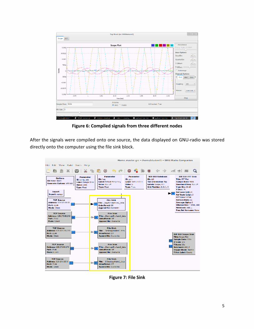
Figure 6: Compiled signals from three different nodes

After the signals were compiled onto one source, the data displayed on GNU-radio was stored

directly onto the computer using the file sink block.

Figure 7: File Sink

6

After the data was collected on the computer, the files were then converted to raw binary data

to MATLAB format using python. The data was then analyzed using MATLAB. The absolute

value, real portion, imaginary portion were all plotted versus time. The frequency (scaled

version of FFT plot) was also plotted on a graph.

Below are the locations at which the signal was transmitted and received from O-CORNET.

Figure 9: Parking Garage Locations

Figure 8: Drillfield Locations

7

Obstacles:

Throughout this research, there have been many obstacles encountered. The main obstacle

was the unreliability of O-CORNET. Due to the system still in the process of being completed,

there were many problems that arose. As a result of this, a main portion of our research

consisted of fixing the nodes and figuring out why the system was not operational. It was found

that many of the nodes had hardware issues and had software that were not compatible with

one another. Another problem that arose with O-CORNET was the fact that the nodes were not

all time synchronized and do not have a GPS implemented in their system. Although an

attempt was made to install GPS onto O-CORNET, it has been, so far, unsuccessful. Another

obstacle was the reliability of the transmitter. Initially a USRP was used to transmit the signal

to O-CORNET but the power level was too weak and was not detected by the nodes and the

computer more than fifty percent of the time. Using a USRP also meant that a mobile power

source would have to be acquired in order to transmit the signal outdoors. In addition to the

aforementioned obstacles, it was also quite a task obtaining a license for MATLAB and working

with python and MATLAB due to the unfamiliarity of the language. To automatically sync the

nodes, a python file had to be created. Python was also used to convert information from

GNU-Radio output, raw binary data, to a readable file in MATLAB, MAT file.

Results and Conclusion:

This project was mostly successful in setting

up O-CORNET for future use. The received

signal shapes (figure 2) were consistent with

the signal that was transmitted. Since there

was no major loss from the file conversion,

the code can be easily modified to look at

the potential correlation between signal

shape and location.

Figure 10: One node

8

The results for the power levels were

consistent with the expected outcome. The

nodes closest to the transmitted had a

higher relative power (figure 3). When the

real vs. imaginary were plotted, the graph

(figure 4) showed rough circles from each

node. The diameter of which corresponds to

the power level of each node.

Since these transmissions were line of sight

with a sinusoidal wave, the result was

expected to resemble the unit circle.

This means, the code that was used to

obtain the information was correct. In order

to look at specific parameters, slight

modifications would have to be

made. However, the basic foundation has

been laid for future work.

Future Work:

Due to the numerous obstacles encountered in this study, future work would include more

consistency between the nodes of O-CORNET. To do this, O-CORNET would have to have all the

proper software (GNU-Radio Companion) installed on all the nodes and all the hardware issues

fixed. Another area that would be address in the future is the accuracy of the transmitter.

Initially, a USRP was used as a transmitter, but due to its unreliability, the rogue walkie talkie

was used instead. Another replication of this study would include a more accurate, higher

power, and programmable transmitter to control the shape, length, and power of the signal

being transmitted. Hopefully, through future studies, it can be determined if there is a

correlation between signal shape and location.

Figure 11: Line of Sight

Figure 12: Three Nodes

9

Outdoor CORNET Tutorial

Ethel Baber, Virginia Polytechnic Institute and State University Danielle Ho, Virginia Polytechnic Institute and State University

Thomas Vormittag, Northern Arizona University

10

TABLE OF CONTENTS

INTRODUCTION ........................................................................... 11

CREATE AN ACCOUNT ON O-CORNET ......................................... 11

SETTING UP GNU RADIO ON YOUR COMPUTER .......................... 11

USING GNU RADIO ...................................................................... 11

ACCESSING THE NODES ............................................................... 15

USING GNURADIO-COMPANION ON A NODE ............................. 16

SIMULATING A NODE .................................................................. 20

SIMULATING MULTIPLE NODES ................................................... 27

RUNNING THE NODES FROM YOUR COMPUTER ......................... 30

CODE ........................................................................................... 33

CONVERTING YOUR DATA INTO MATLAB FILES........................... 37

GEDIT CODE ................................................................................ 38

ANALYZE WITH MATLAB .............................................................. 38

11

Introduction Outdoor Cognitive Radio Network Testbed (O-CORNET) is an infrastructure on the Virginia Tech campus used to test applications with multiple nodes to simulate real world conditions. At the time this was written there were twelve nodes placed on various buildings around campus. The testing conducted by this group used three nodes: Whittemore, Hahn1, and Hahn 2. This document will discuss how to set up the nodes to be used for localization. You will need a Linux based operating system to do this tutorial. This project was done using the open source operating system (OS) Ubuntu http://www.ubuntu.com/. You can either download it to a flashdrive and boot your computer into the OS or download a virtual machine (you can download a free virtual machine) to run the OS on your PC/Mac OS.

Create an account on O-CORNET

To accomplish this, you must email Vuk Marojevic at maroje@vt.edu He will set up your

account and send you a password that must be entered each time you access a node.

Setting up GNU Radio on your computer

If you already have GNU Radio installed, proceed to Step 3. GNU Radio is a free & open-source

software development toolkit that provides signal processing blocks to implement software

radios. A valuable resource is: http://gnuradio.org/redmine/projects/gnuradio/wiki

GNU Radio is the toolkit we used for this project and is highly recommended to succeed at

transmitter localization. If GNU Radio is not installed on your Linux OS the link to install it is

here: http://gnuradio.org/redmine/projects/gnuradio/wiki/InstallingGR.

You will need sudo (administrative) privileges to install it. If you do not have sudo access, you

will need to speak to an admin to help you.

Using GNU Radio

Once you have GNU Radio you may begin by typing gnuradio-companion into the terminal:

After you type this, you should see a blank flow graph that looks like this:

Figure 1: Opening GNU Radio

12

Now you can begin building the flow graph that will connect the node to your computer. The

finished flow block should look like this:

Things to note:

1. The Options block (top left corner) gives you an ID option. This is the name your

python file will be saved as.

2. The 3 Parameter blocks are variables used within the Scope Sink and FFT Sink

blocks. This is useful when you have multiple blocks with the same parameters.

The sample rate MUST be above 196,000! If you use anything less, GNU radio

will set the sample rate to a default which will give you problems later.

3. The WX GUI Notebook organizes the Scope Sink and FFT Sink blocks into one

GUI with 2 tabs

Figure 2: Blank Flow Graph

Figure 3: Collecting Data

13

4. The WX GUI Scope Sink block allows the user to see the signal plotted as relative

power vs. time. The WX GUI FFT Sink block allows the user to see the signal

plotted as relative power vs. frequency.

5. The TCP Source is a way for the user to collect information from the node. The

address must contain the IP address of the server (in this case Whittemore), a

unique port number preferably between 20000 and 60000 (anything lower than

20000 may already be in use), and the mode MUST to be set to client if you have

a dynamic IP address (which all non-servers do).

6. The File Sink saves the data coming from the TCP Source to a file that you

specify on your computer. Save it in an easily accessible place. Once you create

the File Sink disable it by clicking on it and typing D. You will not need it until

later.

The WX GUI FFT Sink and WX GUI Scope Sink are not necessary for this project because the

data will be analyzed in Matlab; however, they are highly recommended. It will be easier to

ensure you are receiving a signal if you have the Scope Sink open.

Parameters for the WX GUI FFT Sink are on the next page.

Figure 4: FFT Parameters

14

Things to note:

1. It’s a good idea to keep the type complex. It will be easier to graph complex data.

2. Sample Rate and Baseband Freq are the variables that were defined in the

parameters you created earlier. Change the Parameter blocks rather than the

local parameters

3. The FFT size adjusts the resolution of the display. As you increase the FFT size

the resolution increases as well

4. Having Average on reduces the noise seen on the plot. Keep on if your signal is

weak.

5. Window Size is number of pixels that will display plots. Change as necessary.

6. Notebook takes in the name of the notebook you defined earlier (nb0) and

places the FFT Sink in tab 2. The numbering of tabs starts at 0.

Parameter for the WX GUI Scope Sink:

Figure 5: Scope Parameters

15

Things to note:

1. V Scale correlates to the y-axis. You will want to change this parameter

depending on the amplitude of your signal. A higher amplitude signal will need a

larger value and vice versa.

2. T Scale correlates to x-axis in time. If the value is set too low, it will be difficult to

see when your signal starts and ends. If too high, the Scope Sink will appear to

be lagging. Adjust accordingly.

3. If Window Size is set in another GUI, it will not have to be redefined. Be sure not

to set it to a conflicting window size. The Notebook is the same as the FFT Sink;

however, the tab number is set to 0 to correlate to tab 1.

Once you’re satisfied with your flow graph save it in an easily accessible place. This will be

important later!

Accessing the Nodes

While it is not required to set up a flow graph, on your computer, before accessing the nodes, it

is important based on the flow graphs to come. To get started we will access the Whittemore

node. Once you have figured out how to access one node, it will be the same process for each

additional node. Begin by opening a terminal (command prompt) and typing the following

command:

ssh -XC username@ocornet1.ece.vt.edu

Note: Each node is designated by a number that follows @ocornet. 1 is used to access

Whittemore. The other nodes will be explained later.

Ex: ssh –XC txlreu@ocornet1.ece.vt.edu

Note: When you type in your password it will appear that you aren’t typing anything in. This is

just the way Linux handles passwords.

Figure 6 : Accessing Whittemore Node

16

The first time you log on you will get a message that looks something like this:

Type yes

Once you type in your password, the terminal will look like this:

Using gnuradio-companion on a Node

As in Step 3, type: gnuradio-companion

Tip: Linux has a feature that completes the command for you if it understands what you’re

asking it to do.

It looks like this:

Figure 7: Authentication

Figure 8: Now Connected to Whittemore

Figure 9: GNU Radio Companion Command

Figure 10: Short Cut Part 1

17

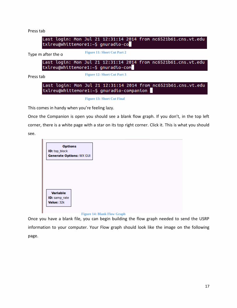
Press tab

Type m after the o

Press tab

This comes in handy when you’re feeling lazy.

Once the Companion is open you should see a blank flow graph. If you don’t, in the top left

corner, there is a white page with a star on its top right corner. Click it. This is what you should

see.

Once you have a blank file, you can begin building the flow graph needed to send the USRP

information to your computer. Your Flow graph should look like the image on the following

page.

Figure 11: Short Cut Part 2

Figure 12: Short Cut Part 3

Figure 13: Short Cut Final

Figure 14: Blank Flow Graph

18

Things to note:

1. The Options block (top right corner) gives you an ID option. This is the name

your python file will be saved as.

2. The 3 Parameter blocks allow you to set variables that will be used in the UHD:

USRP Source. In this case there is only one block, so it is not pivotal to use

parameters, but it is a good habit to form.

3. Be sure to use the correct IP address in the TCP Sink. The IP address shown is

what has been assigned to Whittemore. Make sure the port numbers match

between the TCP Sink on the Whittemore node and the TCP Source on your

computer. If they do not, you will not receive information from the USRP Source.

The Mode MUST be set to Server. This is because the Whittemore node has a

static IP address, your computer does not.

4. You might be wondering how to get the IP address for the node you’re on. If you

type ifconfig in the terminal on the node, like so:

Figure 15: TCP Sink

Figure 16: Ifconfig Command

19

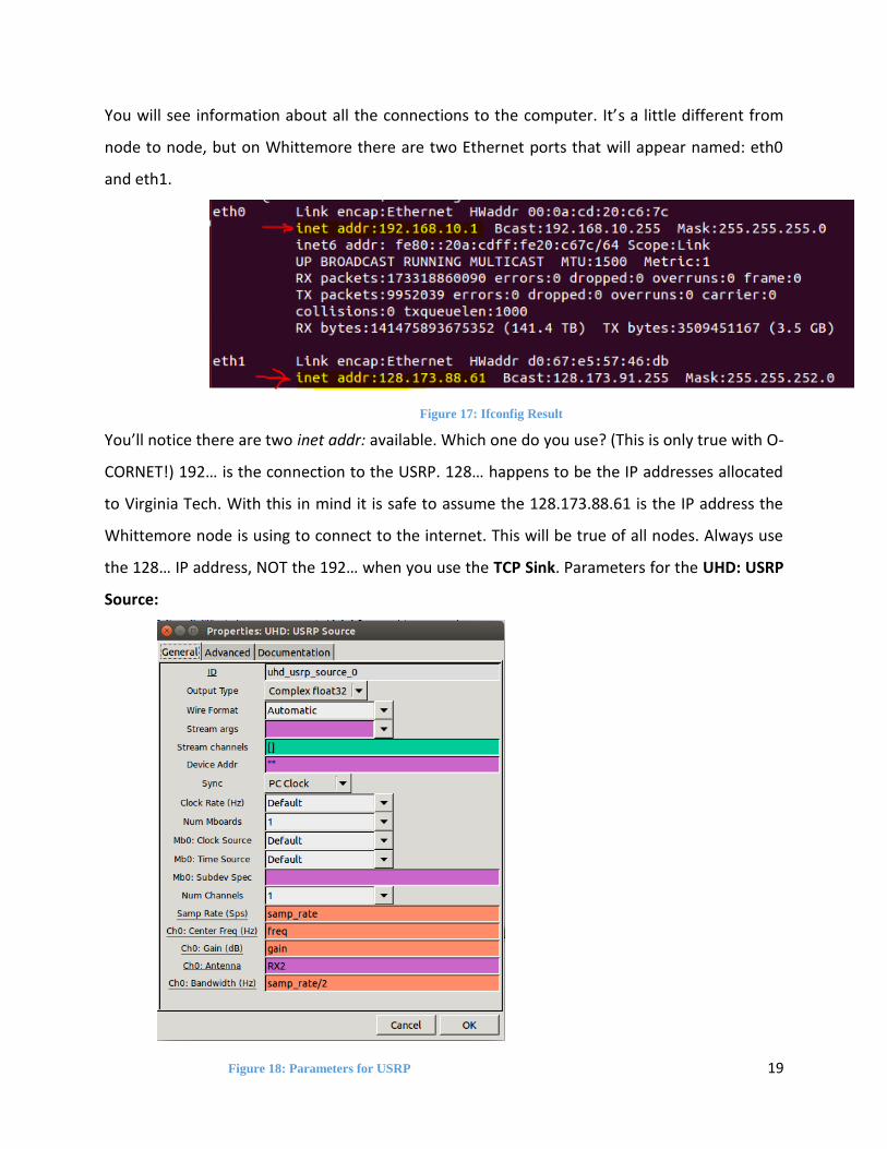
You will see information about all the connections to the computer. It’s a little different from

node to node, but on Whittemore there are two Ethernet ports that will appear named: eth0

and eth1.

You’ll notice there are two inet addr: available. Which one do you use? (This is only true with O-

CORNET!) 192… is the connection to the USRP. 128… happens to be the IP addresses allocated

to Virginia Tech. With this in mind it is safe to assume the 128.173.88.61 is the IP address the

Whittemore node is using to connect to the internet. This will be true of all nodes. Always use

the 128… IP address, NOT the 192… when you use the TCP Sink. Parameters for the UHD: USRP

Source:

Figure 17: Ifconfig Result

Figure 18: Parameters for USRP

20

Things to Note:

1. The Sync parameter is set to PC Clock. In our experience, this did nothing to sync

the nodes because the PC Clocks were different for different nodes. There might

be another option available called unknown PPS. This only appears if the node

has GPS capabilities. When this document was written some nodes had GPS

capabilities others didn’t. If the node you’re working with has an unknown PPS

option, USE IT!! Ideally this will synchronize the nodes in time.

2. The Samp Rate, Center Freq, and Gain should all be set to the parameters you

set previously.

3. The Antenna parameter has 2 options: TX/RX or RX2. If you need to transmit set

it to TX/RX, if you only need to receive set it to RX2. Unless you use Holden or

Durham 2. They do not have auxiliary antennas so use the TX/RX port instead.

4. In the figure above, the Bandwidth is set to half the samp_rate. You may change

this parameter, but insure it is less than the Samp Rate.

Simulating a node

Now that you have a flow graph to collect data from the Whittemore node and a flow graph to

save the data on your computer, you can run the two to see what a signal looks like on the

Whittemore node. If you’ve followed the tutorial, you may have noticed the frequency

parameter is set to 467.5e6. The reason for this is our group used a hand held walkie talkie to

run our simulations. The frequency of the transmitter is… (You guessed it) 467.5 MHz if you do

not have a transmitter handy, you can always look at the frequency of a local radio station or

the Verizon band (751e6).

Note: Be sure to transmit on a band that you are allowed to. If it’s not an open band or you

don’t have a license for it, DO NOT TRANSMITT ON THAT BAND!!! If you disrupt a licensed

transmitter, the FCC will find you and you could get into legal trouble.

The first thing you will need to do is log onto the Whittemore node if you’re not already on it.

Refer back to Step 4 to log on. Once you’re on, run the flow graph. There are two ways to do

this. First is, open the gnuradio-companion and click the gear to compile. The red arrow in the

image on the next page points to the gear.

21

A python file should pop up that looks like this:

The first time you run the flow graph there will be warnings prompting you to resize ports, if

you do not have sudo privileges, you’ll need an admin to resize the ports. If you are unable to

resize the ports, don’t worry too much about it.

If you see the window open and then immediately close, something is wrong. What we found

to work in this case is to close the GNU Radio Companion and return to the terminal. In the

terminal you will need to type the command killall python:

If there aren’t any python files running, no process found will pop up.

Figure 19: TCP Sink Flow Graph

Figure 20: Python Start

Figure 21: Clearing Python Files

22

The second method to run your flow graph is by calling the python file explicitly. When you

create the flow graph, a python file is created that. The python file is what is being used to run

the flow graph. You can run the python file by typing the following:

Note: The python file will only run if you are in the correct directory. If you run the command

but it does not compile type ls in the terminal:

This will display all the files that are in the directory you are in:

If you do not see the python file you’re trying to run, you’ll need to change directory. You can

do this by typing cd <name of directory>/

For example: if I want to switch to the REU_data directory:

You can type ls to see if the file you’re looking for is in the new directory.

Generally files will be a different color than directories. In the above figure, you’ll notice

directories are blue and python files are green, while grc files are white.

To leave a directory type cd ..

Figure 22: Running Python File

Figure 23: Check Directory Command

Figure 25: Changing Directory

Figure 26: Leaving Directory

Figure 24: Example Directory

23

Once you are able to run the python file you should see:

Note: If you need to stop running the python file while it is executing, type ctrl c into the

terminal. A message will open up that looks like this:

If you were unable to change the port sizes, you will see several UHD Warning messages. Ignore

them.

With the flow graph running on Whittemore, return back to the flow graph you have open on

your computer. If you do not have the flow graph, you created in step 3, open it up.

On the flow graph, click the gears in the top toolbar.

Figure 27: Python File Running

Figure 28: Python Execution

24

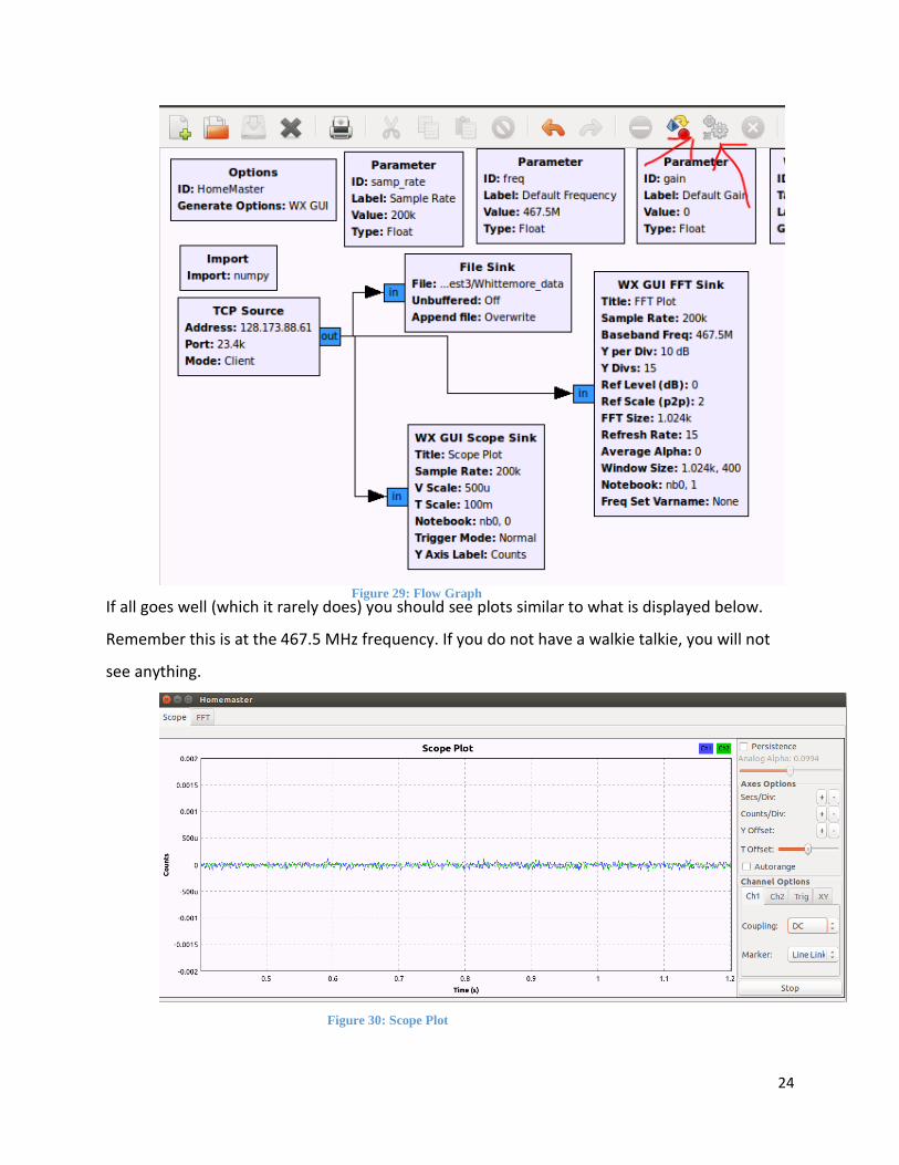
If all goes well (which it rarely does) you should see plots similar to what is displayed below.

Remember this is at the 467.5 MHz frequency. If you do not have a walkie talkie, you will not

see anything.

Figure 29: Flow Graph

Figure 30: Scope Plot

25

This is what the noise floor looks like when nothing is being received on the scope plot.

As soon as I turn on the transmitter, Whittemore receives the signal and displays it in the GUI.

When you run it, you will see the signal as it moves through time.

This is the noise floor of the FFT plot on Whittemore. You may notice there is a peak in the

center of the plot. This is due to reflections from the antenna itself. Just note there is nothing

Figure 31: Signal on Scope Plot

Figure 32: Noise Floor

26

you can do to stop it. Since this happens you may want to offset your center frequency by a

little. So we were transmitting at 467.5625 MHz with our walkie talkie, therefore we set the

center frequency to 467.5 MHz. This put the reflection far enough away from the area we were

looking at that it would not interfere with our signal.

As soon as the transmitter is activated, we see a spike in the FFT plot at the frequency of our

transmitter.

The second method to running the plots is to run the python command explicitly. This is the

same as running it on the node. First figure out where your python file is. Once you know that,

cd into it and run it like you did before: python <name of python file>.py

You will see the same thing as in the plots above, but without having to manually click on the

compile button in the companion.

Figure 33: Signal on FFT Plot

27

Simulating multiple nodes

This table will come in handy for the TCP Source information:

Node O-CORNET number IP address

Whittemore 1 128.173.88.61

Durham 1 2 128.173.92.242

Holden 3 128.173.206.233

Durham 2 4 128.173.93.170

Hahn 1 5 128.173.156.114

Hahn 2 6 128.173.156.115

Newman 7 128.173.126.5

Now that you have managed to retrieve the information on the Whittemore node, you can

collect the same information from multiple nodes. You will need a flow graph, similar to the

one you created on Whittemore, on each node you wish to access. The process is the same for

each node; however, you do not need to recreate the flow graphs you created on Whittemore.

You can simply send them to the other nodes you wish to collect data on. To send a file from

one node to another you can use the command

scp <file name to send> username@ocornet<node you want to send to>.ece.vt.edu:

For example: scp Whittemore_slave.grc txlreu@ocornet5.ece.vt.edu This is being sent to Hahn1

node

You will be prompted for your password then details about the file transfer will be displayed

Table 1: O-CORNET IP Addresses

Figure 34: Password Promt

Figure 35: File Details

28

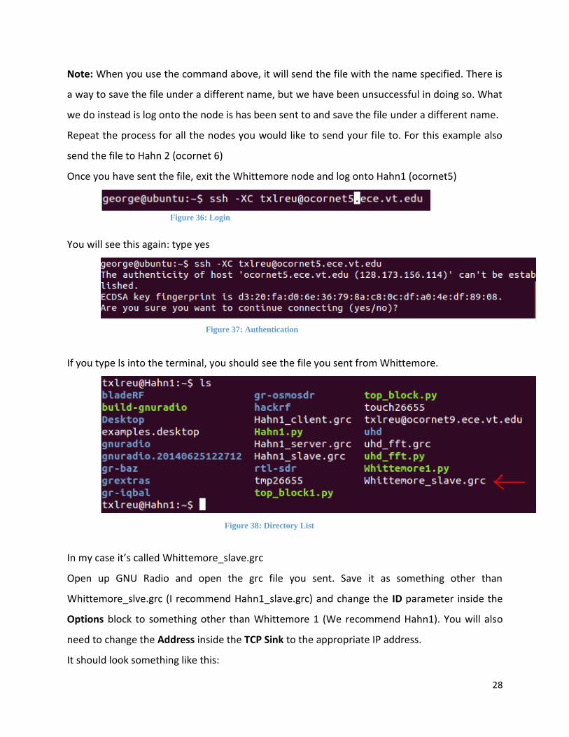
Note: When you use the command above, it will send the file with the name specified. There is

a way to save the file under a different name, but we have been unsuccessful in doing so. What

we do instead is log onto the node is has been sent to and save the file under a different name.

Repeat the process for all the nodes you would like to send your file to. For this example also

send the file to Hahn 2 (ocornet 6)

Once you have sent the file, exit the Whittemore node and log onto Hahn1 (ocornet5)

You will see this again: type yes

If you type ls into the terminal, you should see the file you sent from Whittemore.

In my case it’s called Whittemore_slave.grc

Open up GNU Radio and open the grc file you sent. Save it as something other than

Whittemore_slve.grc (I recommend Hahn1_slave.grc) and change the ID parameter inside the

Options block to something other than Whittemore 1 (We recommend Hahn1). You will also

need to change the Address inside the TCP Sink to the appropriate IP address.

It should look something like this:

Figure 36: Login

Figure 37: Authentication

Figure 38: Directory List

29

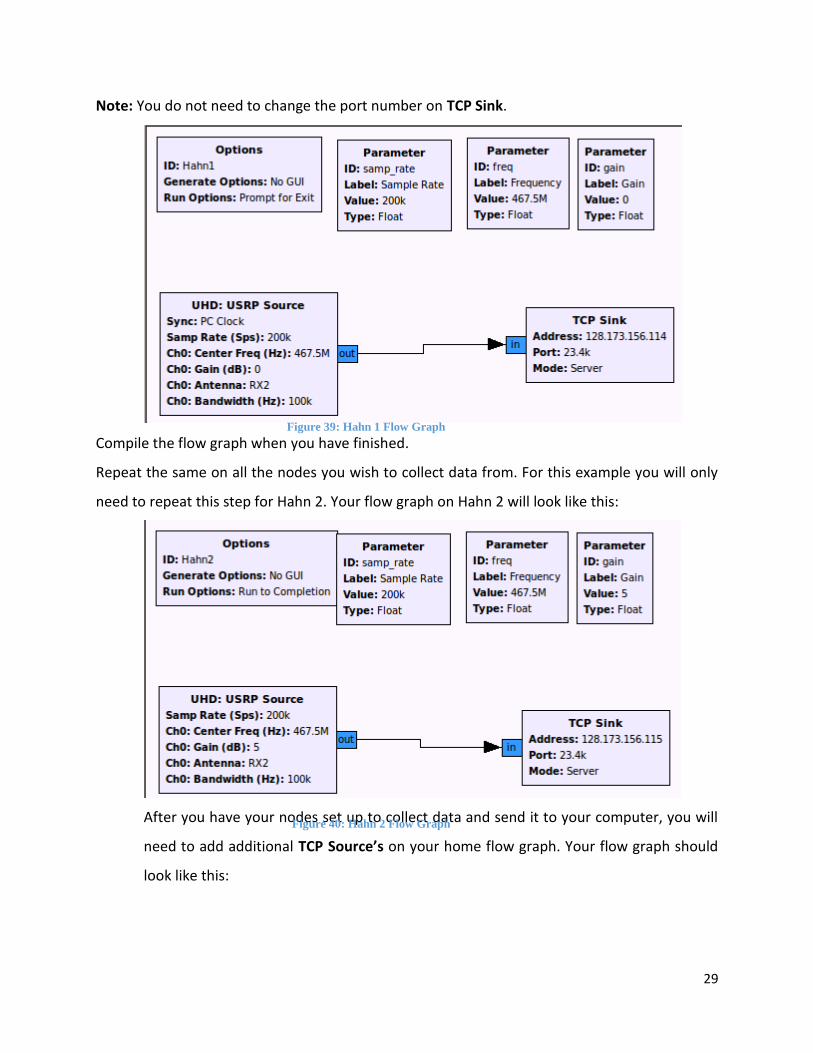
Note: You do not need to change the port number on TCP Sink.

Compile the flow graph when you have finished.

Repeat the same on all the nodes you wish to collect data from. For this example you will only

need to repeat this step for Hahn 2. Your flow graph on Hahn 2 will look like this:

After you have your nodes set up to collect data and send it to your computer, you will

need to add additional TCP Source’s on your home flow graph. Your flow graph should

look like this:

Figure 39: Hahn 1 Flow Graph

Figure 40: Hahn 2 Flow Graph

30

Things to Note:

1. The Simplest way to add a TCP Source and File Sink is to copy and paste

2. Be sure to change the File name to something unique for each sink

3. If you want to see the output of your file, double click on the Scope Sink and

change Num Inputs to 3.

Compile the flow graph.

Running the nodes from your computer

Now that you have all your nodes set up with appropriate flow graphs and python files, you can

write some code to run all the nodes in a python file.

Figure 41: TCP Source Flow Graph

31

The first thing you should do is open the python file you created with the flow graph above. The

python file will be the name you defined in the ID parameter under the Options block. If you

did not give it a unique name, the default is top_block. You can open the python file by typing

nautilus in the home directory and searching for your file manually.

You can also cd into the directory you saved your flow graph and type gedit with the file name.

The file will open in text editor called gedit. You will see a ton of code you may not understand,

don’t worry about that. Once you’re in gedit, click on Edit in the toolbar. Scroll down to

Preferences and click it.

Change the tab width to 4. For some weird reason, the default is 8.

Figure 42: File Search-Manual

Figure 43: File Search-gedit

Figure 44: Preferences Location

32

You can also display line numbers in the View tab, if you wish.

The command you will be using to establish an automatic link is the paramiko command. You

need to install the library before you can import it. To do this use the sudo apt-get install

python-pip on your computer. If you do not have sudo privilages, you will need to talk to your

admin.

Type y

Figure 45: Preferences

Figure 46: Confirmation

33

Once it has installed type pip install paramiko into your terminal

For background on the paramiko command and to see example this website is useful:

http://jessenoller.com/blog/2009/02/05/ssh-programming-with-paramiko-completely-different

Now that you have the paramiko package you can remotely connect to the nodes by copying

and pasting the following code into a blank python script file:

Code

from gnuradio import blocks

from gnuradio import eng_notation

from gnuradio import gr

from gnuradio import wxgui

from gnuradio.eng_option import eng_option

from gnuradio.fft import window

from gnuradio.filter import firdes

from gnuradio.wxgui import fftsink2

from gnuradio.wxgui import scopesink2

from grc_gnuradio import blks2 as grc_blks2

from grc_gnuradio import wxgui as grc_wxgui

from optparse import OptionParser

import numpy

import wx

from HomeMaster import HomeMaster

import paramiko

import time

if __name__ == '__main__':

import ctypes

import sys

if sys.platform.startswith('linux'):

try:

x11 = ctypes.cdll.LoadLibrary('libX11.so')

x11.XInitThreads()

except:

print "Warning: failed to XInitThreads()"

parser = OptionParser(option_class=eng_option, usage="%prog: [options]")

34

parser.add_option("", "--freq", dest="freq", type="eng_float",

default=eng_notation.num_to_str(467.5e6),

help="Set Default Frequency [default=%default]")

parser.add_option("", "--gain", dest="gain", type="eng_float", default=eng_notation.num_to_str(0),

help="Set Default Gain [default=%default]")

parser.add_option("", "--samp-rate", dest="samp_rate", type="eng_float",

default=eng_notation.num_to_str(32e3),

help="Set Sample Rate [default=%default]")

(options, args) = parser.parse_args()

# Code to connect you to the nodes

ssh = paramiko.SSHClient() #Establishes connection to the SSHClient

ssh.set_missing_host_key_policy(paramiko.AutoAddPolicy()) #Accounts for potential errors

#Connects to the Whittemore node

ssh.connect('ocornet1.ece.vt.edu', username='txlreu', password='********')

#The passwords have been commented out for obvious reasons

print 'Starting Remote Server 1'

stdin1, stdout1, stderr1 = ssh.exec_command("python Whittemore1.py")

time.sleep(3)

#Connects to the Hahn 1 node

print 'Starting Remote Server 5'

ssh.connect('ocornet5.ece.vt.edu', username='txlreu', password='********')

stdin5, stdout5, stderr5 = ssh.exec_command("python Hahn1.py")

time.sleep(3)

#Connects to the Hahn 2 node

print 'Starting Remote Server 6'

ssh.connect('ocornet6.ece.vt.edu', username='txlreu', password='********')

stdin6, stdout6, stderr6 = ssh.exec_command("python Hahn2.py")

time.sleep(3)

#Connects to the Newman node

#ssh.connect('ocornet7.ece.vt.edu', username='txlreu', password='********')

#print 'Starting Remote Server 7'

#stdin7, stdout7, stderr7 = ssh.exec_command("python Newman1.py")

#time.sleep(3)

35

#Connects to the Hutchenson node

#ssh.connect('ocornet9.ece.vt.edu', username='txlreu', password='********')

#print 'Starting Remote Server 9'

#stdin9, stdout9, stderr9 = ssh.exec_command("python Hutchenson1.py")

#time.sleep(3)

#Connects to the Williams 1 node

#ssh.connect('ocornet11.ece.vt.edu', username='txlreu', password='********')

#print 'Starting Remote Server 11'

#stdin11, stdout11, stderr11 = ssh.exec_command("python Williams1.py")

#time.sleep(3)

print 'Starting Local Scope'

tb = HomeMaster(freq=options.freq, gain=options.gain, samp_rate=options.samp_rate)

tb.Start(True)

tb.Wait()

#Holds the connection open while you collect data

while True:

print stdout1.readline() #Command for Whittemore

print stdout5.readline() #Command for Hahn 1

print stdout6.readline() #Command for Hahn 2

#print stdout7.readline() #Command for Newman

#print stdout9.readline() #Command for Hutchenson

#print stdout11.readline() #Command for Williams 1

Save the file as rx_runner.py

Within ssh.connect('ocornet1.ece.vt.edu', username='txlreu', password='********') you will

need to type your username and password where it says username and password.

In the terminal run the rx_runner file by typing python rx_runner.py. If the python file is not in

the directory you’re in, you will need to cd into it.

When you run the python file, you will see “Starting Remote Server 1” in the terminal followed

by “Starting Remote Server 5”, “Starting Remote Server 6”. This will take about 10 seconds.

Afterward you should see the WX GUI Scope Sink with 6 different channels. There are 3

channels per USRP. It should look something like the image on the next page.

36

When the signal is detected, the Scope will show the signal like this:

The different sine waves show what is being detected by the different nodes. Because I am

closer to Whittemore than I am Hahn, the Whittemore node is detecting the signal at a higher

rate than either of the Hahn nodes.

The figure below is what you should see in the terminal after you close the Scope GUI.

Figure 47: Multi-Channel Noise Floor

Figure 48: Multi-Channel-Signal Detected

37

Converting your data into Matlab files

If you do not have Matlab installed on your computer, this step is useless to you. The File Sinks

you hooked up to each TCP Source will be used now. If you look in the directory you defined

when you set your File sink, you will notice a file has been created under the name you

specified. Depending on how long you ran the rx_runner file, this file may be quiet large. What

you will do now is convert the data from binary information to a mat file. You’re doing this so

you can analyze the data in Matlab.

The language you’ll be using to do the conversion is called octave. It is basically a free version of

Matlab that you will need to install.

Then

Figure 49: Terminal Display

Figure 50: Octave Installation

Figure 51: Octave Update

38

It will take a few minutes.

To convert the files, first open a blank document in gedit and paste the following code:

Gedit Code

addpath("/home/wireless/gnuradio/gr-utils/octave") #adds path of octave file

#Converts the data from binary to complex numbers

Whittemore_oct = read_complex_binary("/home/student1/REU/GarageTest3/Whittemore_data");

#Be sure to change the path

save("-v7","Whittemore_exp1.mat","Whittemore_oct")

#the first parameter is a matlab thing, the second parameter is what you want to save the file as in

matlab, the third parameter is the name of the file being converted.

Hahn1_oct = read_complex_binary("/home/student1/REU/GarageTest3/Hahn1_data");

save("-v7","Hahn1_exp1.mat","Hahn1_oct")

Hahn2_oct = read_complex_binary("/home/student1/REU/GarageTest3/Hahn2_data");

save("-v7","Hahn2_exp1.mat","Hahn2_oct")

Things to Note:

1. Be sure to change the path to your specific directory

2. Change read_complex_binary to the directory you specified in the File Sink

Save the file as a .mat file. I saved it as convert.mat

Run it by typing octave

Once the data has been converted to a mat file you can open it up in Matlab.

Analyze with Matlab

After you have converted the data into a .mat file format, you can few it in matlab by typing:

A = import(‘Whittemore_exp1.mat);

B = import(‘Hahn1_exp1.mat);

C = import(‘Hahn2_exp1.mat);

This imports the data into an array. From there you can analyze the data in whatever way suits

your needs.

Figure 52: Run Convert File