Outdoor Mapping and Navigation using Stereo Vision - SRIagrawal/iser06.pdf · Outdoor Mapping and...

Outdoor Mapping and Navigation using Stereo Vision

Kurt Konolige, Motilal Agrawal, Robert C. Bolles, Cregg Cowan, Martin Fischler,and Brian Gerkey

Artificial Intelligence Center, SRI International, Menlo Park, CA [email protected]

1 IntroductionWe consider the problem of autonomous navigation in an unstructured outdoor envi-ronment. The goal is for a small outdoor robot to come into a new area, learn aboutand map its environment, and move to a given goal at modest speeds (1 m/s). Thisproblem is especially difficult in outdoor, off-road environments, where tall grass,shadows, deadfall, and other obstacles predominate. Not surprisingly, the biggestchallenge is acquiring and using a reliable map of the new area. Although workin outdoor navigation has preferentially used laser rangefinders [13, 2, 6], we usestereo vision as the main sensor. Vision sensors allow us to use more distant objectsas landmarks for navigation, and to learn and use color and texture models of theenvironment, in looking further ahead than is possible with range sensors alone.

In this paper we show how to build a consistent, globally correct map in realtime, using a combination of the following vision-based techniques:

• Efficient, precise stereo algorithms. We can perform stereo analysis on 512x384images in less than 40 ms, enabling a fast system cycle time for real-time obstacledetection and avoidance.

• Visual odometry for fine registration of robot motion and corresponding obstaclemaps. We have developed techniques that run at 15 Hz on standard PC hardware,and that provide 4% error over runs of 100 m. Our method can be integratedwith information from inertial (IMU) and GPS devices for robustness in difficultlighting or motion situations, and for overall global consistency.

• A fast RANSAC [3] method for finding the ground plane. The ground planeprovides a basis for obstacle detection algorithms in challenging outdoor terrain,and produces high-quality obstacle maps for planning.

• Learning color models for finding paths and extended ground planes. We learnmodels of the ground plane and path-like areas on and off-line, using a combina-tion of geometrical analysis and standard learning techniques.

• Sight-line analysis for longer-range inference. Stereo information on our robot isunreliable past 8m, but it is possible to infer free space by finding “sight lines”to distant objects.

2 Outdoor Mapping and Navigation

Good map-building is not sufficient for efficient robot motion. We have devel-oped an efficient global planner based on previous gradient techniques [10], as wellas a novel local controller that takes into account robot dynamics, and searches alarge space of robot motions.

While we have made advances in many of the areas above, it is the integrationof the techniques that is the biggest contribution of the research. The validity of ourapproach is tested in blind experiments, where we submit our code to an independenttesting group that runs and validates it on an outdoor robot. In the most recent tests,we finished first out of a group of eight teams.

1.1 System overview

This work was conducted as part of the DARPA Learning Applied to GroundRobotics (LAGR) project. We were provided with two robots (see Figure 1, eachwith two stereo devices encompassing a 110 degree field of view, with a baselineof 12 cm. The robots are near-sighted: depth information degrades rapidly after 6m.There is also an inertial unit (IMU) with angular drift of several degrees per minute,and a WAAS-enabled GPS. There are 4 Pentium-M 2 GHz computers, one for eachstereo device, one for planning and map-making, and one for control of the robotand integration of GPS and IMU readings. In our setup, each stereo computer per-forms local map making and visual odometry, and sends registered local maps to theplanner, where they are integrated into a global map. The planner is responsible forglobal planning and reactive control, sending commands to the controller.

In the following sections, we first discuss local map creation from visual input,with a separate section on learning color models for paths and traversable regions.Then we examine visual odometry and registration in detail, and show how consistentglobal maps are created. The next section discusses the global planner and localcontroller. Finally, we present performance results for several tests in Spring 2006.

Fig. 1. Left: LAGR robot with two stereo sensors. Right: Typical outdoor scene as a montagefrom the left cameras of the two stereo devices.

1.2 Related work

There has been an explosion of work in mapping and localization (SLAM), mostof it concentrating on indoor environments [7, 11]. Much of the recent research onoutdoor navigation has been driven by DARPA projects on mobile vehicles [2]. The

Outdoor Mapping and Navigation 3

sensor of choice is a laser rangefinder, augmented with monocular or stereo vision.In much of this work, high-accuracy GPS is used to register sensor scans; exceptionsare [6, 13]. In contrast, we forego laser rangefinders, and explicitly use image-basedregistration to build accurate maps. Other approaches to mapping with vision are[18, 19], although they are not oriented towards realtime implementations. Obstacledetection using stereo has also received some attention [18]. There have been a num-ber of recent approaches to visual odometry [15, 16]. Our system is distinguished byrealtime implementation and high accuracy using a small baseline in realistic terrain.We discuss other examples of related work in the text.

2 Local map constructionThe object of the local map algorithms is to determine, from the visual information,which areas are freespace and which are obstacles for the robot: the local map. Notethat this is not simply a matter of geometric analysis – for example, a log and a rowof grass may have similar geometric shapes, but the robot can traverse the grass butnot the log.

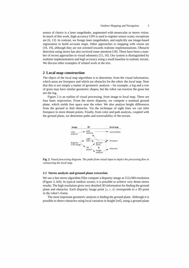
Figure 2 is an outline of visual processing, from image to local map. There arefour basic trajectories. From the stereo disparity, we compute a nominal groundplane, which yields free space near the robot. We also analyze height differencesfrom the ground to find obstacles. Via the technique of sight lines we can inferfreespace to more distant points. Finally, from color and path analysis, coupled withthe ground plane, we determine paths and traversability of the terrain.

analysiscolor

(1/d) imagedisparity

points3D

linessight

planeground

analysisheight

analysispath

3Dimage

traversibility

obstacles

freespace

local map

Fig. 2. Visual processing diagram. The paths from visual input to depict the processing flow inconstucting the local map.

2.1 Stereo analysis and ground plane extraction

We use a fast stereo algorithm [9]to compute a disparity image at 512x384 resolution(Figure 3, left). In typical outdoor scenes, it is possible to achieve very dense stereoresults, The high resolution gives very detailed 3D information for finding the groundplane and obstacles. Each disparity image point [u, v, d] corresponds to a 3D pointin the robot’s frame.

The most important geometric analysis is finding the ground plane. Although it ispossible to detect obstacles using local variation in height [ref], using a ground plane


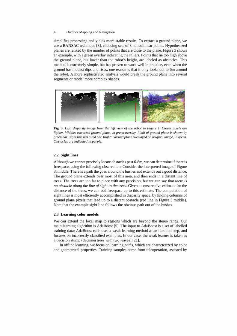
simplifies processing and yields more stable results. To extract a ground plane, weuse a RANSAC technique [3], choosing sets of 3 noncollinear points. Hypothesizedplanes are ranked by the number of points that are close to the plane. Figure 3 showsan example, with a green overlay indicating the inliers. Points that lie too high abovethe ground plane, but lower than the robot’s height, are labeled as obstacles. Thismethod is extremely simple, but has proven to work well in practice, even when theground has modest dips and rises; one reason is that it only looks out to 6m aroundthe robot. A more sophisticated analysis would break the ground plane into severalsegments or model more complex shapes.

Fig. 3. Left: disparity image from the left view of the robot in Figure 1. Closer pixels arelighter. Middle: extracted ground plane, in green overlay. Limit of ground plane is shown bygreen bar; sight line has a red bar. Right: Ground plane overlayed on original image, in green.Obstacles are indicated in purple.

2.2 Sight lines

Although we cannot precisely locate obstacles past 6-8m, we can determine if there isfreespace, using the following observation. Consider the interpreted image of Figure3, middle. There is a path the goes around the bushes and extends out a good distance.The ground plane extends over most of this area, and then ends in a distant line oftrees. The trees are too far to place with any precision, but we can say that there isno obstacle along the line of sight to the trees. Given a conservative estimate for thedistance of the trees, we can add freespace up to this estimate. The computation ofsight lines is most efficiently accomplished in disparity space, by finding columns ofground plane pixels that lead up to a distant obstacle (red line in Figure 3 middle).Note that the example sight line follows the obvious path out of the bushes.

2.3 Learning color models

We can extend the local map to regions which are beyond the stereo range. Ourmain learning algorithm is AdaBoost [5]. The input to AdaBoost is a set of labelledtraining data; AdaBoost calls uses a weak learning method as an iteration step, andfocuses on incorrectly classified examples. In our case, the weak learner is taken asa decision stump (decision trees with two leaves) [21].

In offline learning, we focus on learning paths, which are characterized by colorand geometrical properties. Training samples come from teleoperation, assisted by


an automatic analysis of the route and prospective paths. We sample images at ap-proximately one meter intervals; since our robot is well-localized by visual odometry,we can project the route of the robot on each of the sampled images and calculatethe distance of each pixel from the route centerline. Figure 4(b) shows the projectedroute of the robot in red. The green region corresponds to pixels which are 2 metersor closer to the robot’s trajectory. This route corresponds to the robot’s traversal onthe mulch path shown in Figure 4(a). For each image, we form a gaussian modelof the normalized color in several regions close to the robot, and use this model toclassify all pixels in the image. If the classified region conforms to a path-like shape,we use it as input to the learning algorithm. Figure 4(c) shows the geometrical pathin yellow.

(a) Original image (b) Robot’s route (c) Geometrical path

Fig. 4. Illustration of offline learning.

Once the pixels belonging to the path are marked in each image, we use two-classAdaBoost to learn the color models for path and non-path pixels. From the model,we construct an RGB lookup table for fast classification, using AdaBoost on eachcolor triplet in the table. During online runs, classification of a pixel is a simple tablelookup.

We can also use this algorithm for online learning of more general terrain. We usethe current image and the corresponding ground plane/obstacles marked by stereowithin close range to classify the pixels beyond stereo range in the same image. Thisis a standard two class classification problem - the two classes being ground planeand obstacles. We use the AdaBoost algorithm (described before) to learn these twoclasses and then classify the pixels beyond the stereo range.

2.4 Results

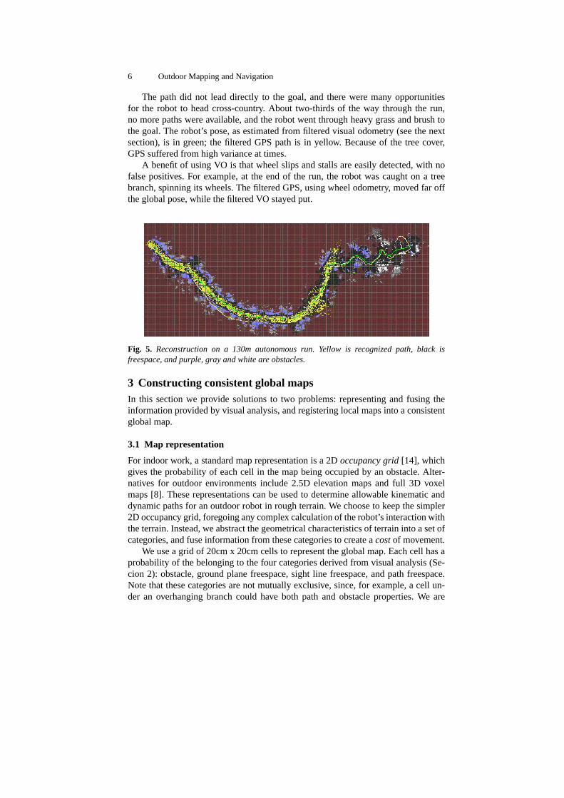
The combined visual processing results in local maps that represent traversabilitywith a high degree of fidelity. Figure 5 shows the results of an autonomous run ofabout 130m, over a span of 150 seconds. We used offline learning of mulch paths ona test site, then used the learned models on the autonomous run. The first part of therun was along a mulch path under heavy tree cover, with mixed sunlight and deepshadows. Cells categorized as path are shown in yellow; black is freespace. Obstaclesare indicated by purple (for absolute certainty), and white-to-gray for decreasingcertainty. We did not use sight lines for this run.


The path did not lead directly to the goal, and there were many opportunitiesfor the robot to head cross-country. About two-thirds of the way through the run,no more paths were available, and the robot went through heavy grass and brush tothe goal. The robot’s pose, as estimated from filtered visual odometry (see the nextsection), is in green; the filtered GPS path is in yellow. Because of the tree cover,GPS suffered from high variance at times.

A benefit of using VO is that wheel slips and stalls are easily detected, with nofalse positives. For example, at the end of the run, the robot was caught on a treebranch, spinning its wheels. The filtered GPS, using wheel odometry, moved far offthe global pose, while the filtered VO stayed put.

Fig. 5. Reconstruction on a 130m autonomous run. Yellow is recognized path, black isfreespace, and purple, gray and white are obstacles.

3 Constructing consistent global mapsIn this section we provide solutions to two problems: representing and fusing theinformation provided by visual analysis, and registering local maps into a consistentglobal map.

3.1 Map representation

For indoor work, a standard map representation is a 2D occupancy grid [14], whichgives the probability of each cell in the map being occupied by an obstacle. Alter-natives for outdoor environments include 2.5D elevation maps and full 3D voxelmaps [8]. These representations can be used to determine allowable kinematic anddynamic paths for an outdoor robot in rough terrain. We choose to keep the simpler2D occupancy grid, foregoing any complex calculation of the robot’s interaction withthe terrain. Instead, we abstract the geometrical characteristics of terrain into a set ofcategories, and fuse information from these categories to create a cost of movement.

We use a grid of 20cm x 20cm cells to represent the global map. Each cell has aprobability of the belonging to the four categories derived from visual analysis (Se-cion 2): obstacle, ground plane freespace, sight line freespace, and path freespace.Note that these categories are not mutually exclusive, since, for example, a cell un-der an overhanging branch could have both path and obstacle properties. We are


interested in converting these probabilities into a cost of traversing the cell. If theprobabilities were mutually exclusive, we would simply form the cost function asa weighted sum. With non-exclusive categories, we chose a simple prioritizationschedule to determine the cost. Obstacles have the highest priority, followed byground plane, sight lines, and paths. Each category has its own threshold for signifi-cance: for example, if the probability of an obstacle is low enough, it will be ignoredin favor of one of the other categories. The combination of priorities and thresholdsyields a very flexible method for determining costs. Figure 5 shows a color-codedversion of computed costs.

3.2 Registration and visual odometry

The LAGR robot is equipped with a GPS that is accurate to within 3 to 10 meters ingood situations. GPS information is filtered by the IMU and wheel encoders to pro-duce a more stable position estimate. However, because GPS drifts and jumps overtime, it is impossible to differentiate GPS errors from other errors such as wheel slip-page, and the result is that local maps cannot be reconstructed accurately. Considerthe situation of Figure 6. Here the robot goes through two loops of 10m diameter.There is a long linear feature (a low wall) that is seen as an obstacle at the begin-ning and end of the loops. Using the filtered GPS pose, the position of the wall shiftsalmost 2m during the run, and obstacles cover the robot’s previous tracks.

Fig. 6. Three stages during a run using GPS filtered pose. Obstacle points are shown in white,freespace in black, and the yellow line is the robot’s path. The linear feature is marked byhand in red in all three maps, in its initial pose.

Our solution to the registration problem is to use visual odometry (VO) to ensurelocal consistency in map registration. Over larger regions, filtering VO with GPSinformation provides the necessary corrections to keep errors from growing withoutbounds. We describe these techniques in the next two sections.

The LAGR robot presents a challenging situation for visual odometry: wide FOVand short baseline make distance errors large, and a small offset from the groundplane makes it difficult to track points over longer distances. We have developeda robust visual odometry solution that functions well under these conditions. Webriefly describe it here; for more details consult [1].


Our visual odometry system uses feature tracks to estimate the relative incre-mental motion between two frames that are close in time. Corner feature points aredetected in the left image of each stereo pair and tracked across consecutive frames.Figure 7 illustrates the detection and tracking of feature points in two images. Weuse a RANSAC method to find the best set of matching features. As in the groundplane analysis, any three matched features determine a motion hypothesis; we scorethe hypothesis using the pixel reprojection errors in both the cameras. In a final step,the best motion hypothesis is refined in a nonlinear minimization step.

Fig. 7. Example of visual odometry. Left: dense set of detected features. Right: motion ofsuccessfully tracked features.

The IMU and the wheel encoders are also used to fill in the relative poses whenvisual odometry fails. This happens due to sudden lighting changes, fast turns of therobot or lack of good features in the scene(e.g. blank wall).

3.3 Global consistency

Relative motions between consecutive frames are chained together to obtain the ab-solute pose at each frame. Obviously, this is bound to result in accumulation of errorsand drifting. We use GPS to correct the pose of the vehicle through a simple linearfilter. Pose information is used when the GPS receiver has at least a 3D position fix,and heading information is used only when the vehicle is travelling 0.5 m/s or faster,to limit the effect of velocity noise from GPS on the heading estimate. In addition,GPS measurements are used only if the robot has travelled a minimum distance fromthe last GPS measurement. The filter nudges the VO pose towards global consistency,while maintaining local consistency. Over larger loops, of course, the 3 m deviationof the GPS unit means that the map may not be consistent. In this case, other tech-niques such as wide-baseline image matching [12] would have to be employed.

The quality of the registration from filtered VO, shown in Figure 8, can be com-pared to the filtered GPS of Figure 6. The low wall, which moved almost 2m overthe short loops when using GPS, is much more consistent when VO is employed.And in cases where GPS is blocked or degraded, such as under heavy tree cover inFigure 5, VO still produces maps that are locally consistent. It also allows us to de-termine wheel slips and stalls with almost no false positives – note the end of the run


Run Number 1 2 3 4Distance(meters) 82.4 141.6 55.3 51.0Method Percentage Error

Vehicle Odometry 1.3 11.4 11.0 31.0Raw Visual Odometry 2.2 4.8 5.0 3.9Visual Odometry & GPS 2.0 0.3 1.7 0.9

Table 2. Loop closure error.

Test 12 Test 13BL SRI BL SRI

Run 1 5:25 1:46 5:21 2:28Run 2 5:34 1:50 5:04 2:12Run 3 5:18 1:52 4:45 2:12

Table 3. Run times for base-line (BL) and SRI.

in Figure 5, where the robot was hung up and the wheels were slipping, and wheelodometry produced a large error.

Fig. 8. VO in the same sequence as Figure 6. GPS filtered path in yellow, VO filtered path isin green.

3.4 Results of visual odometry

We have implemented and tested our integrated pose system on several outdoor ter-rains. Since GPS is accurate to only about 3-4 meters, in order to validate our results,the robot was moved in a closed loop on a typical outdoor environment over 50–100m, and used the error in start and end poses.

Table 2 compares this error for vehicle odometry (IMU + wheel odometry), vi-sual odometry and the GPS integrated visual odometry for four loops. Except forthe first loop, visual odometry outperforms the vehicle odometry, even without GPSfiltering, and is comparable to the std of GPS (3m). VO substantially outperformedodometry in 3 of the 4 loops, mainly because of turns and wheel slippage duringthose runs. This is especially evident in loop 4, where the robot was slipping in mudfor a substantial amount of time.

4 Planning and ControlThe LAGR robot was provided with a “baseline” system that used implementationsof D∗ [20] for global planning and DWA [4] for local control. Using this system,we (as well as other teams) had frequent crashes and undesirable motion. The maincauses were the slowness of the planner and the failure of the controller to sufficientlyaccount for the robot’s dynamics.


We replaced the baseline system with a global gradient planner and a localtrajectory-rollout controller, both described below. This system safely controls theLAGR robot at its maximum speed of 1.3 m/s, with the robot flawlessly negotiatingmaze-like obstacle courses at an average speed of 1.1 m/s.

4.1 Global planning

For global planning, we re-implemented a gradient planner [10, 17] that computesoptimal paths from the goal to the robot, given the cost map. The algorithm hasseveral unique modifications:

• Unlike other implementations, it uses a true Euclidean metric, rather than a Man-hattan or diagonal metric.

• The calculation is extremely efficient, using threshold-based queues, rather thana best-first update, which has high overhead.

• It computes the configuration space for a circular robot, and includes safety dis-tances to obstacles.

• Rapid switching of global paths is avoided by including hysteresis - lowering thecost along the path.

Typically we run the global planner within a subregion of the whole map, sincethe robot is continuously moving towards the goal and encountering new areas. Onlonger runs, up to 200m, we use an 80m x 80m area; the global planner runs in about30 ms in this region. The global planner is conservative in assuming the robot tobe circular, with a diameter equal to the length of the robot. Also, it does not takeinto account the nonholomic nature of the robot’s motion. Instead, we rely on a localcontroller to produce feasible driving motions.

4.2 Local control

Given the global cost information produced by the planner, we must decide whatlocal controls to apply to the robot to drive it toward the goal. Algorithms such asDWA compute these controls by first determining a target trajectory in position orvelocity space (usually a circular arc or other simple curve), then inverting the robot’sdynamics to find the desired velocity commands that will produce that trajectory.

We take the opposite approach: instead of searching the space of feasible trajec-tories, we search the space of feasible controls. As is the case with most differentially-driven platforms, the LAGR robot is commanded by a pair (x, θ) of translational androtational velocities. The 2-D velocity space is bounded in each dimension by limitsthat reflect the vehicle’s capabilities. Because we are seeking good, rather than op-timal, control, we sample, rather than exhaustively search, this rectangular velocityregion. We take a regular sampling (∼25 in each dimension, ∼625 total), and foreach sample simulate the effect of applying those controls to the robot over a shorttime horizon (∼2s).

The simulation predicts the robot’s trajectory as a sequence of 5-D (x, y, θ, x, θ)states with a discrete integral approximation of the vehicle’s dynamics, notably theacceleration limits. The resulting trajectories, projected into the (x, y) plane, are


smooth, continuous, 2-D curves that, depending on the acceleration limits, may notbe easily parameterizable (e.g., for the LAGR robot, the trajectories are not circulararcs). Each simulated trajectory t is evaluated by the following weighted cost:

C(t) = αObs + βGdist + γPdist + δ1

x2

where Obs is the sum of grid cell costs through which the trajectory takes the robot;Gdist and Pdist are the estimated shortest distances from the endpoint of the tra-jectory to the goal and the optimal path, respectively; and x is the translational com-ponent of the velocity command that produces the trajectory. This cost calculation isvery fast because the computation of cell costs and distances was done by the plan-ner, allowing the controller to access them via table lookup. We choose the trajectoryt for which C(t) is minimized, which leads our controller to prefer trajectories that:(a) remain far from obstacles, (b) go toward the goal, (c) remain near the optimalpath, and (d) drive fast. Trajectories that bring any part of the robot into collisionwith a lethal obstacle are discarded as illegal.

5 PerformanceFor the LAGR program, the independent testing group ran monthly blind demos ofthe perception and control software developed by eight teams and compared theirperformance to a baseline system. The last three demos (11, 12, and 13) were con-sidered tests of performance from the first 18 months of the program. The SRI Teamwas first in the last two tests (Test 12 and 13), after begin last in Test 11. Most of theproblems in Test 11 were caused by using the baseline planner and controller, andwe switched to the one described in the paper for Tests 12 and 13. Figure 3 shows thetimes for the runs in these tests. We achieved the short run times in Tests 12 and 13through a combination of precise map building, high-speed path planning, and care-ful selection of robot control parameters. Our average speed was over 1.1 m/s, whilethe robot top speed was limited to 1.3 m/s. Map building relied on VO to providegood localization, ground-plane analysis to help detect obstacles, and sight lines toidentify distant regions that are likely to be navigable.

6 ConclusionWe have demonstrated a complete autonomous system for off-road navigation inunstructured environments, using stereo vision as the main sensor. The system isvery robust - we can typically give it a goal position several hundred meters away,and expect it to get there. But there are hazards that are not dealt with by the methodsdiscussed in this paper: water and ditches are two robot-killers. Finally, we would liketo use visual landmarks to augment GPS for global consistency, because it wouldgive finer adjustment in the robot’s position, which is critical for following routesthat have already been found.

References

1. M. Agrawal and K. Konolige. Real-time localization in outdoor environments using stereovision and inexpensive gps. In Intl. Conf. of Pattern Recognition (ICPR), 2006. To appear.


2. P. Bellutta, R. Manduchi, L. Matthies, K. Owens, and A. Rankin. Terrain perception forDEMO III. In Proc. of the IEEE Intelligent Vehicles Symp., 2000.

3. M. Fischler and R. Bolles. Random sample consensus: a paradigm for model fitting withapplication to image analysis and automated cartography. Commun. ACM., 24:381–395,1981.

4. D. Fox, W. Burgard, and S. Thrun. The dynamic window approach to collision avoidance.IEEE Robotics and Automation Magazine, 4(1):23–33, 1997.

5. Y. Freund and R. E. Schapire. A decision-theoretic generalization of on-line learning andan application to boosting. J. of Computer and System Sciences, 55(1):119–139, 1997.

6. J. Guivant, E. Nebot, and S. Baiker. High accuracy navigation using laser range sensorsin outdoor applications. In ICRA, 2000.

7. J. S. Gutmann and K. Konolige. Incremental mapping of large cyclic environments. InCIRA, 1999.

8. K. Iagnemma, F. Genot, and S. Dubowsky. Rapid physics-based rough-terrain rover plan-ning with sensor and control uncertainty. In ICRA, 1999.

9. K. Konolige. Small vision systems: hardware and implementation. In Intl. Symp. onRobotics Research, pages 111–116, 1997.

10. K. Konolige. A gradient method for realtime robot control. In IROS, 2000.11. J. J. Leonard and P. Newman. Consistent, convergent, and constant-time slam. In IJCAI,

2003.12. D. G. Lowe. Distinctive image features from scale-invariant keypoints. Intl. J. of Com-

puter Vision, 60(2):91–110, 2004.13. M. Montemerlo and S. Thrun. Large-scale robotic 3-d mapping of urban structures. In

ISER, 2004.14. H. Moravec and A. Elfes. High resolution maps for wide angles sonar. In ICRA, 1985.15. D. Nister, O. Naroditsky, and J. Bergen. Visual odometry. In CVPR, 2004.16. C. F. Olson, L. H. Matthies, M. Schoppers, and M. W. Maimone. Robust stereo ego-

motion for long distance navigation. In CVPR, 2000.17. R. Philippsen and R. Siegwart. An interpolated dynamic navigation function. In ICRA,

2005.18. A. Rankin, A. Huertas, and L. Matthies. Evaluation of stereo vision obstacle detection

algorithms for off-road autonomous navigation. In AUVSI Symp. on Unmanned Systems,2005.

19. D. J. Spero and R. A. Jarvis. 3D vision for large-scale outdoor environments. In Proc. ofthe Australasian Conf. on Robotics and Automation (ACRA), 2002.

20. A. Stentz. Optimal and efficient path planning for partially-known environments. InICRA, volume 4, pages 3310–3317, 1994.

21. P. Viola and M. Jones. Rapid object detection using a boosted cascade of simple features.In CVPR, pages 511–518, 2001.

Outdoor Mapping and Navigation using Stereo Vision - SRIagrawal/iser06.pdf · Outdoor Mapping and...

Documents

Transcript of Outdoor Mapping and Navigation using Stereo Vision - SRIagrawal/iser06.pdf · Outdoor Mapping and...