Outcrop Prediction Problem 1

IntroductionOutcrop prediction is based on the concept of intersecting a planar surface (geological contact) with an irregular surface (topographic surface). In reality this occurs in 3D however the final depiction is on a 2D topographic map. The underlying assumption is that the geological contact or surface is a perfect plane. In many undeformed geological terranes this assumption is a valid over relatively small areas such as a 1:24K quadrangle. The value of the method is that it predicts on the topographic surface where the geological plane outcrops. This has obvious value in the case of a planar fault surface, or planar water table surface. If the method is applied to both the upper and lower planar contacts of a bed the result will be the predicted outcrop belt of the bed. The method also yields a structure contour map of the planar surface. This combined with the topographic map can be used to predict the depth below the ground surface of the plane at any point on a map – an obvious advantage when attempting to estimate costs of drilling wells or overburden removal in mining.

Geometrical RelationshipsWhether the outcrop prediction is done “analog” with traditional orthographic projections, or “digital” with computer CAD/GIS, the fundamental process is the same – contouring a geological plane and then comparing those contours to the topographic contours. The structure contours of the geological plane will be straight lines, with the spacing between lines a function of the dip angle (inclination) of the plane:

s = ci / tan(α)

where s is the perpendicular distance between adjacent structure contours, α is the dip angle of the plane, and ci is the topographic contour interval. The elevation value of the structure contour always decreases by the contour interval value (ci) in the dip direction.

If the outcrop of the structural plane occurs at a topographic elevation equal to a contour interval, the “s” spacing can be used from that point to construct all necessary structure contours as a set of parallel lines. If a contact can be traced on a map surface from aerial photography or from a geological map the “starting” structure contour can be set to where a topographic contour crosses the contact line. However, this may not be possible so the relationship:

Tan (α) = (Δy)/(Δx)

Can be used to calculate the exact offset from the control point to start the structure contour. For example, assume that the map topographic contour interval is 20 feet, and a bedding plane contact with attitude 330, 55 SW is discovered at 707 feet elevation. A 720 topographic contour is near the outcrop so the offset from the outcrop to the 720 structure contour on the contact is needed. First you should realize that the offset direction from the outcrop is in the 030 because that is perpendicular to strike and in the “up-dip” direction (i.e. elevation is gained from 707 to 720). The amount of map distance between the outcrop and 720 structure contour is calculated from:

Tan(55) = 13/x

x = 13/Tan(55) = 9.1 feet

Where x is the offset distance from the outcrop to the 720 structure contour. From this offset point the 720 structure contour can be drawn as a straight line striking 330. Where this line intersects the 720 topographic contour would generate outcrop control points.

From the structure contour map the elevation of any point on the geological surface can be estimated, and this generates three possible scenarios when compared to the topographic contours/surface:

1. The point is above the topographic surface (i.e. its elevation is higher than the topographic surface at that point) indicating that the geological plane has been eroded.

2. The point is below the topographic surface (i.e. its elevation is lower than the topographic surface at that point) indication that the erosional surface is above the geological plane.

3. The point on the geological plane is equal to the elevation of the topographic surface indicating the outcrop position of the plane. The line connecting these points is the trace of the outcrop on the map.

Therefore, whether the process is accomplished manually or digitally finding the points where the structure contours intersect the matching topographic contours will trace out the outcrop pf the structural plane.

If the outcrop position of the top and bottom of a tabular unit (i.e. top and bottom contacts are planar and parallel) are known, then the two sets of contours would allow tracing the contact of both planes across the topography. In this case the area between the two traces is the outcrop belt of the unit. Alternatively, if the outcrop position and orientation of the bottom of the unit where known, and the bedding thickness was measured and can be assumed to be constant, the structure contours of the top of the bed can be predicted by:

w = t / sin(α)

where w is the perpendicular distance between structure contours of equal value between the top and bottom contacts, t is the thickness of the bed, and α is the dip angle. The unit structural top contour would be offset “w” distance from the bottom contact equivalent contour in the dip direction. The spacing between adjacent top contact contours would be the same as calculated for the bottom contact because they both have the same dip and dip direction. Having both sets of structure contours overlaying the topographic contours can cause a map to become overly “complex” so whether the process is manual or digital it is advisable to use different color for each set. Figure 1 displays a topographic contour map of the USA campus at a 5-foot contour interval (black contour lines), and a structure contour map of the bottom of a planar clay unit (blue contour lines) using the same 5-foot contour interval. The dip angle of 1.43 degrees yields a spacing between adjacent structure contours of 200 feet. As you can see in Figure 1, the map can be “complex” even with only one set of structure

contours superimposed on the topographic contours. As you can imagine to process of tracking where structure contours intersect the same elevation topographic contour is tedious, time consuming, and error-prone. In other words, a perfect task for a computer!

Using QGIS to Process Outcrop PredictionThe good news about outcrop prediction is this- QGIS can easily solve the outcrop prediction problem using its built-in tools. The steps for calculating the outcrop of a planar geological surface with ArcGIS are summarized below:

Step 1: Add base map features to QGIS project. Don’t forget to create a folder for this project and store only files related to this project in that folder. If you are working on a USA workstation it is advisable to work on a flash drive.

Step 2: Use the Python programs “PlaneTrendSurf.py” to generate an elevation grid of the top geological plane based on its outcrop position and orientation. If you need to solve a 3-point problem do this now because you will need the trend and plunge of the true dip as input into this program. If necessary do the same for the other contact if modelling a tabular unit.

Step 3: Use “Raster Math” from the “Raster” menu to subtract the topographic grid from the planar surface grid to produce “residual” rasters for top and bottom contacts.

Step 4: Reclassify both of the of the residual raster features produced in step 3 into simplified raster features where the pixel value “1” represents strata above the contact plane (i.e. negative residuals), and “2” represents strata below the contact (i.e. positive values). (Toolbox: SAGA > Raster Tools > Reclassify Values).

Step 5: Use “Toolbox: SAGA > Raster Tools > Reclassify Values ” to add together the two rasters produced in step 4. The composite will contain three possible pixel values: 2=strata above top contact, 3=strata between bottom and top contact, and 4=strata below bottom contact.

Step 6: Use the following steps to convert the raster geologic map created in step 5 to a true “polygon” feature:

a. Use GRASS: “r.contour.step” to produce contours at 2.5 and 3.5 as a 1st approximation of the contacts.

b. “Smooth” the contours from the above step with GRASS: “v.generalize”. Name this layer contacts.

c. Combine the map border with “contacts” to make a line layer named “union”. Do this with the main menu “Vector > Geoprocessing Tools > Union”.

d. With the “Union” layer use “Toolbox: QGIS geoalgorithms > Vector Geometry Tools > Polygonize” to create a smooth polygon topology for the geologic map. Name this layer “Lithology”.

e. Use “Properties > Style” to assign color to the geologic map.

Problem 1: Generating an Outcrop Prediction from a 3-Point Problem and Thickness MeasurementIn this problem you will be given a digital topographic map containing 3 outcrop points for the top of a tabular stratigraphic unit. You will also be given a raster grid that represents the topographic surface of the map area. The thickness of the tabular unit is 50 feet. Make a geologic map of the map area that displays the predicted outcrop extent of the tabular stratigraphic unit in red, older strata in green, and younger strata in blue. Answer the questions at the end of this document using QGIS tools.

Step 1: Create a Project File and Add Starting Files FeaturesYou can access all of the starting files at the GIT 461/561 online site under the “Resources” section. For this exercise you will need the following files:

OP_prob1_start.zip {QGIS geodatabase file containing starting feature class data}

PlaneTrendSurf.py {Python program for generating a planar trend surface grid}

Plane_matrix.xlsm {Excel program that calculates the attitude of a planar surface from 3 control points}

Alternatively you can download the above files from this web site if you don’t have a USA online account:

http://www.usouthal.edu/geography/allison/gy461/gy461_project_resources.htm

Create a working folder on your own flash drive and download the above starting files to this folder.

In the “OP_prob1_start.zip” geodatabase file are the following starting features:

Border: map boundary

Topocontours: topographic contours

Outcrops: outcrop points for the top contact

Topopts3D: elevation survey control points used to generate the DEM

ElevTINgrd2: DEM (elevation grid) of the map area.

You should add all of the above items to the project file. The coordinates of these features are in Alabama State Plane West (feet). Figure 2 displays the QGIS project file with these features added to the project. Make sure that the coordinate system for the project file is set to projected coordinate system Alabama State Plane West Zone NAD27 (feet). The (X,Y,Z) points are the outcrop positions of the top of the tabular stratigraphic unit. At this time use the “Identify” button in the button bar to identify the coordinates of the 3 outcrop points.

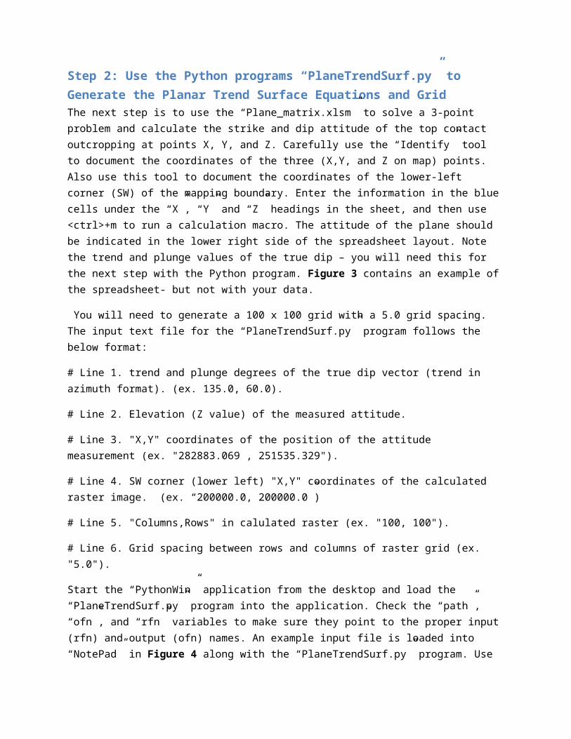
Step 2: Use the Python programs “PlaneTrendSurf.py” to Generate the Planar Trend Surface Equations and GridThe next step is to use the “Plane_matrix.xlsm” to solve a 3-point problem and calculate the strike and dip attitude of the top contact outcropping at points X, Y, and Z. Carefully use the “Identify” tool to document the coordinates of the three (X,Y, and Z on map) points. Also use this tool to document the coordinates of the lower-left corner (SW) of the mapping boundary. Enter the information in the blue cells under the “X”, “Y” and “Z” headings in the sheet, and then use <ctrl>+m to run a calculation macro. The attitude of the plane should be indicated in the lower right side of the spreadsheet layout. Note the trend and plunge values of the true dip – you will need this for the next step with the Python program. Figure 3 contains an example of the spreadsheet- but not with your data.

You will need to generate a 100 x 100 grid with a 5.0 grid spacing. The input text file for the “PlaneTrendSurf.py” program follows the below format:

# Line 1. trend and plunge degrees of the true dip vector (trend in azimuth format). (ex. 135.0, 60.0).

# Line 2. Elevation (Z value) of the measured attitude.

# Line 3. "X,Y" coordinates of the position of the attitude measurement (ex. "282883.069 , 251535.329").

# Line 4. SW corner (lower left) "X,Y" coordinates of the calculated raster image. (ex. “200000.0, 200000.0”)

# Line 5. "Columns,Rows" in calulated raster (ex. "100, 100").

# Line 6. Grid spacing between rows and columns of raster grid (ex. "5.0").

Start the “PythonWin” application from the desktop and load the “PlaneTrendSurf.py” program into the application. Check the “path”, “ofn”, and “rfn” variables to make sure they point to the proper input (rfn) and output (ofn) names. An example input file is loaded into “NotePad” in Figure 4 along with the “PlaneTrendSurf.py” program. Use the “File > Run” menu option to generate the ASCII grid file for the top contact. The output file will be whatever you named it in the source code. In this example the ASCII grid file is "prob1_top_grd.txt".

You will need to generate the bottom contact ASCII grid to complete the project but note that you do not have any outcrop control points as you did for the top. Remember that you can assume the unit is tabular to the bottom contact will have the same attitude. You also know that the thickness is 50 feet. Sketch out a cross-section of the problem to see if you can figure out how to modify the input file for the top contact to correctly generate the bottom contact ASCII grid file (HINT: only one number in the top contact input file needs to be changed to make the bottom contact input file). The data in the two input files are summarized below:

Top Contact Input File

Line 1: {dip direction azimuth} , {Dip Angle} (get these from the spreadsheet)

Line 2: {elevation of control point} (use point X on the map, elevation = 1000)

Line 3: {x coordinate} , {y coordinate} (use “Identify” too to get this from the map at point X)

Line 4: 200000.0, 200000.0 (x,y coordinates of the SW corner of the grid)

Line 5: 100, 100 (number of columns and rows in grid)

Line 6: 5.0 (spacing between grid node points)

Bottom Contact Input File

Line 1: {dip direction azimuth} , {Dip Angle} (get these from the spreadsheet)

Line 2: {elevation of control point} (1000 – thickness/cos(dip angle) )

Line 3: {x coordinate} , {y coordinate} (use “Identify” too to get this from the map at point X)

Line 4: 200000.0, 200000.0 (x,y coordinates of the SW corner of the grid)

Line 5: 100, 100 (number of columns and rows in grid)

Line 6: 5.0 (spacing between grid node points)

After generating the ASCII text file grids they can be added to the project with “Layer > Add Layer > Add Vector Layer”.

Step 3: Generate Raster Residuals by Subtracting the Topographic DEM from each Contact DEM.Use “Raster > Raster Calculator” to subtract the elevation grid (“ElevTINgrd2”) from the top contact grid (“PlaneGridTop”) and name the residuals result as “resid_top”. Remember that any grid values less than zero should be where strata above the top contact outcrops, and values greater than zero will be where the strata below the top contact outcrops. Be sure to check the results with the “Identify Features” tool on the main toolbar. A left click with this tool will identify the x,y,z coordinates of the “click” for highlighted layer in the layer window. A click near outcrop points X, Y and Z should give residuals near 0 because these are outcrop points.

Use the same methods to generate the “resid_bot” grid (“PlaneGridBot” –“ElevTINgrd2”).

Step 4: Reclassify the Top/Bottom Residuals.To reclassify the two residual grids use the processing toolbox “SAGA > Raster Tools > Reclassify values” tool and start it. In the window dialog select “range” mode and proceed to replace values <= 0.0 with a “1” value, and all other values (i.e. > 0.0) with a “2” value. Figure 4 displays the window dialog filled out with appropriate info for the “reclass_top” raster. Follow the same procedure to create “reclass_bot”.

Step 5: Add the 2 Reclassified Rasters to Produce a Geology Raster.Now use the “Raster Calculator” to add the two reclassified grids together (“reclass_top” + “reclass_bot”) to create a new raster named “GeologyRaster”. This raster will represent the geologic map in the following way:

Top Grid + Bottom Grid = Composite Grid

1 1 2=younger strata exposed

(strata above top and bottom contact)

2 1 3=intermediate strata exposed

(strata below top contact, above bottom contact)

2 2 4=older strata exposed

(strata below top contact, below bottom contact)

Therefore, when the composite pixel values are “2”, younger strata are exposed, “3” means intermediate strata are exposed, and “4” requires that older strata are exposed. Note that the condition of the top grid node = 1 and the bottom grid = 2 at the same map position is not possible if the top contact is structurally above the bottom contact.

The appearance of the “GeologyRaster” is displayed in Figure 5.

Step 6: Convert the raster geologic map to a true “polygon” feature.The “GeologyRaster” visually displays the geologic map of the outcrop prediction but it is not useful for calculations. This step converts the raster to a more useful polygon topology.

Contacts between stratigraphic units are needed to separate the lithologic polygons. Generating contours at 2.5 and 3.5 grid values will accomplish this task. Use the processing tools “GRASS 7 > raster > r.contour.step” and fill in as in Figure 6. These contours are obviously too jagged because they follow the pixel boundaries so they need to be “smoothed”.

Use the processing tools “GRASS 7 > Vector > v.generalize.smooth” to generate “smoothed” from the “contours”. Use the “snakes” method for best results. Figure 7 displays the window dialog for generating the smoothed results.

Invariably the smoothed contours will fall short of intersecting the border so they will have to be edited so they intersect the border. Also a close inspection of the top contact shows that the line just misses the X,Y,Z control points. Start edit mode on the “contacts” layer by clicking on the “Toggle Editing” tool in the main toolbar while the “contacts” layer is selected in the layer window. Note that the vertices of

the contacts will display as a red “cross”. Now from the “Settings” menu select “Snapping options”. From this menu you can set snapping to vertices or line segments and set the tolerance. For now set the tolerance to 3 map units and the snap mode to segments. Also set “snap to visible layers”. Proceed to zoom in to where the contact end points are close to the border. Select a contact line with the “Select features” tool and then select “Node Tool”. Left-click on the contact end point and drag until it snaps to the border. Proceed to snap all contact line end points to the border.

Next use the same methods to drag a contact line vertex to pass through the X,Y,Z data points, however, make sure to set the snap mode to “vertex”.

Now use the “Vector > Geoprocessing > Union” to merge the “Border” and “Contacts” line layers into “Union”. Then use the processing tools “QGIS geoalgorithms > Vector geometry tools > polygonize” to turn the “Union” line layer into “Lithology” polygons. Use the “Properties > Style” for “Lithology” to colorize the different polygons as in Figure 8. Also check out the attribute table of the “Lithology” layer. Note that the area and perimeter columns where automatically added by the previous “Polygonize” operation. The units for area and perimeter are always based on the map coordinate units – feet in this case.

Step 7: Compose Layout for PrintingCompose a map layout using the methods covered in the example problem. The result should closely resemble Figure 9. Print the map at a scale of 1:1000 to turn in for grading along with the answers for the following questions.

Questions

1.1 What is the area of the following units in ft.2 ?a. Younger unit: _________________b. Intermediate unit: ______________c. Older unit: __________

{Hint: check out the attribute table of the “Lithology” polygon layer. Remember that area units are always the linear units of the map coordinate system squared – in this case ft.2.}

1.2 If the intermediate unit could be completely mined within the map area how many metric tons would be removed? Assume an average density of 2.85g/cm3.

________________________ metric tons

{HINT: Find the area of the map where you know both the upper and lower contacts exist in the subsurface. Because you were given the thickness of the unit you can now calculate a volume. Be careful of unit conversions!}

Figure 1: Example map using structure contour method of outcrop prediction.

Figure 2: Appearance of starting map with given data added to the project.

Figure 3: Example of a 3-point problem solved in the spreadsheet.

Figure 4: Reclassify dialog window for creating "reclass_top" layer.

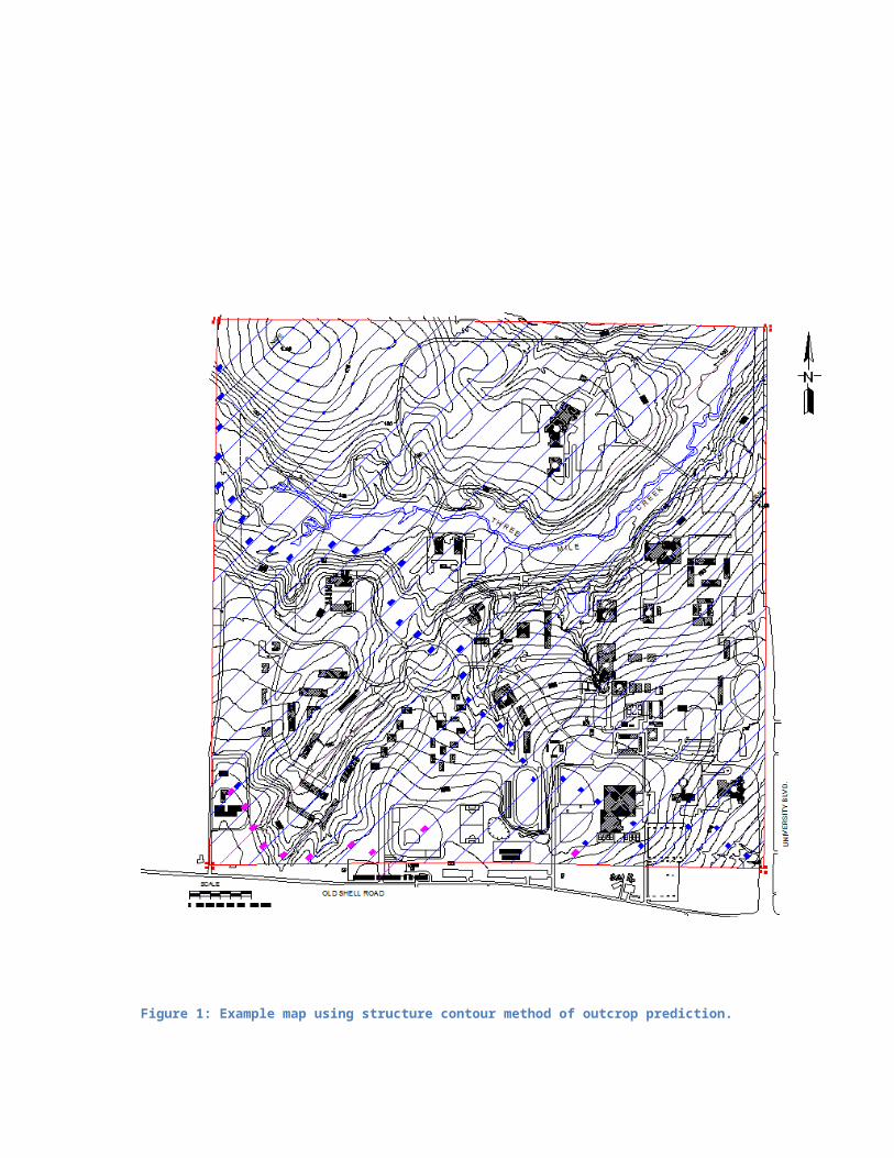
Figure 5: Geology raster results from adding "reclass_top" and "reclass_bot".

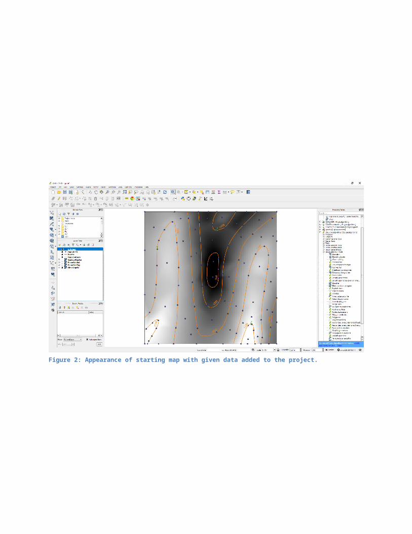
Figure 6: Generation of contact contours from "GeologyRaster".

Figure 7: Window dialog for smoothing contact contours.

Figure 8: Appearance of the lithologic polygons.

Figure 9: Layout of problem 1.