STUDIES IN THE POLITICAL ECONOMY OF LOCALGOVERNMENT

DISSERTATION

Presented in Partial Ful�llment of the Requirements for

the Degree Doctor of Philosophy in the

Graduate School of The Ohio State University

By

Matthew John Holian, B.A., M.A.

* * * * *

The Ohio State University

2008

Dissertation Committee:

Professor Donald Haurin, Adviser

Professor Trevor Brown

Professor Massimo Morelli

Professor Gene Mumy

Approved by

Adviser

Economics GraduateProgram

c Copyright by

Matthew John Holian

2008

ABSTRACT

This dissertation explores topics related to the scope, structure and performance of

local government, how the performance of government in�uences citizen satisfaction,

and how citizen satisfaction in�uences political behavior such as voting. Using both

formal (mathematical) theory and empirical analysis, three essays explore: outsourc-

ing in U.S. cities with an application to emergency ambulance service and elderly

voter interest groups, optimal decentralization in the context of both corporations

and federal systems of government, and citizen evaluations of government perfor-

mance as a determinant of voting turnout. The studies employ a methodological

approach, which is interdisciplinary (with particular emphasis on integrating ideas

from organizational and public economics), and applied theoretic.

ii

To my parents

iii

ACKNOWLEDGMENTS

I owe an immeasurable intellectual debt to Don Haurin and Massimo Morelli, both

of whom sel�essly invested a great deal of time into my scholarly development. The

same can be said of Trevor Brown and Gene Mumy; I was most fortunate to receive

superb advice and training from my entire committee.

Of course without my parents, none of this would have been possible, but my

upbringing was special; both of my parents were teachers and share a love of ideas,

and my father, a sociologist, on every family vacation pointed out what I would later

realize as "the general in the particular."

My wife Bridget kept me both healthy and happy, and taught me many of the

important aspects of life that are not part of the graduate school curriculum.

A number of individuals provided me with speci�c assistance. Tom Miller and

others of the National Research Center graciously provided a portion of the data

from the National Citizen Survey to analyze, and allowed me to reprint their survey

instrument in the appendix. Martha Perego of the International City Manager

Association helped me classify cities as either council-manager or mayor-council.

iv

VITA

March 22, 1981.................................... Born - Parma, Ohio

2004..................................................... M.A. Economics, The Ohio State University

2002..................................................... B.A. Economics, Ohio University

2003 - present...................................... Graduate Teaching and ResearchAssociate, The Ohio State University

PUBLICATIONS

Research Publications

1. M. Holian, "Compstat, Community Policing and the Science of Success:A Market-Based Approach to Police Management." Economic A¤airs, 27, 4, (2007)

FIELDS OF STUDY

Major Field: Economics

v

TABLE OF CONTENTS

Abstract............................................................................................................. iiDedication.......................................................................................................... iiiAcknowledgments.............................................................................................. ivVita.................................................................................................................... vList of Figures.................................................................................................... viiiList of Tables..................................................................................................... ix

Chapters:

1. Introduction............................................................................................. 1

1.1 References........................................................................................ 4

2. Outsourcing in U.S. Cities: Ambulances and Elderly Voters................... 5

2.1 The model........................................................................................ 102.1.1 Preferences and public good production technology........... 102.1.2 Political competition and platform determination.............. 142.1.3 Comparative statics............................................................ 17

2.2 Data and empirical methodology..................................................... 262.3 Conclusion........................................................................................ 422.4 Appendix.......................................................................................... 43

2.4.1 Derivation of w� > w�....................................................... 442.4.2 Derivation of equilibrium g................................................ 452.4.3 Derivation of comparative statics....................................... 452.4.4 Data appendix: JEMS data set.......................................... 472.4.5 Classifying cities as "mayor-council" or "council-manager" 492.4.6 State laws and outsourcing................................................ 51

2.5 References........................................................................................ 52

vi

3. Optimal Decentralization in Corporations and Federations......................... 56

3.1 Models............................................................................................... 583.2.1 M-form Hypothesis.................................................................. 583.2.2 Decentralization Theorem......................................................... 62

3.2 The relation between the M-form Hypothesisand Decentralization Theorem............................................................ 65

3.3 Some extensions to the nested model................................................. 713.3.1 Spillovers in the performance signals: part I........................... 733.3.2 Spillovers in the performance signals: part II.......................... 74

3.4 Conclusion.......................................................................................... 773.5 References.......................................................................................... 773.6 Appendix............................................................................................ 79

3.6.1 Background............................................................................ 793.6.2 Derivation of expected bonus................................................. 813.6.3 Spillovers in the performance signals: part III......................... 833.6.3 Spillovers in the performance signals: part IV......................... 84

4. Dissatisfaction and Turnout: .Evidence from Citizen Satisfaction Surveys................................................. 85

4.1 Theoretical background....................................................................... 894.2 Empirical background and methodology............................................. 1004.3 Conclusion.......................................................................................... 1154.4 References.......................................................................................... 1164.5 Appendix............................................................................................ 119

5. Conclusion.................................................................................................. 130

Bibliography....................................................................................................... 131

vii

LISTS OF FIGURES

Figure

2.1 Tax price and service level................................................................... 232.2 Likelihood of outsourcing and service level.......................................... 233.1 The basic U-form/M-form distinction in a multiproduct,

multifunction �rm................................................................................... 813.2 Centralized versus federal political structure......................................... 814.1 Satisfaction a¤ects four responses; loyalty a¤ects voice....................... 91

viii

LISTS OF TABLES

Table

2.1 E¤ect of variable change on equilibrium service level............................ 202.2 E¤ect of variable change on outsourcing likelihood............................... 262.3 Variables and their theoretical counterparts........................................... 312.4 Summary statistics................................................................................. 322.5 Probit Regressions Using Data from 200 largest US cities, 1990......... 372.6 Probit Regressions Using Data from 200 largest US cities, 2000......... 402.7 Cities use of EMS transport delivery mode, by year............................ 492.8 Probit Regressions Using Data from 200 largest US cities, 1990......... 523.1 g level under three regimes.................................................................... 654.1 Sample population summary statistics, by jurisdiction............................ 1074.2 Summary statistics for individual characteristics..................................... 1094.3 Probit regression, marginal e¤ects reported........................................... 1134.4 Baseline; substituting loyalty for homeownership.................................... 1204.5 Probit regression, marginal e¤ects reported, using statesat..................... 1214.6 Probit regression, marginal e¤ects reported, using fedsat....................... 1224.7 Probit regression, marginal e¤ects reported, using all government levels 123

ix

CHAPTER 1

INTRODUCTION

This dissertation explores topics related to the scope, structure and performance

of local government. On scope, it asks when should a government produce a public

service itself versus procure it through the market? On structure, when is a central-

ized system of government superior to a fragmented system? And on performance,

how do citizen perceptions of government a¤ect political behavior such as voting?

The objective is, using an interdisciplinary perspective, to throw new light onto these

questions, which are among the most enduring in the �eld of political economy.

The themes of scope, structure and performance are also central topics in or-

ganizational economics. Compare two subcategories of the Journal of Economic

Literature (JEL) classi�cation system: H11 - Structure, Scope, and Performance of

Government (a subcategory of the Public Economics category) and L25 - Firm Perfor-

mance: Size, Diversi�cation, and Scope, a subcategory of the Industrial Organization

category. On a methodological level, the aim of this dissertation is to utilize in-

sights from both of these areas. While this dissertation contains three relatively

autonomous chapters, this interdisciplinary theoretical perspective, which lies near

1

the intersection of industrial organization and political economy (or public choice),1

is a unifying strand running among them.

Another unifying strand running through the three essays is the use of formal

theory. Mathematical models here both serve to clarify and generalize key concepts,

which is useful for organizing thoughts about complicated topics.2 Working through

formal models can also lead to new insights, and this use of formal modeling is most

evident in the latter half of chapter three. In addition to formal models, two of

the three chapters (the second and fourth) also include a data analysis component,

and second essay derives some predictions that can be tested in future research; thus

a third commonality between the chapters is a focus on applied theory, which links

formal models with empirical analyses.

Finally, all three essays explore local governments. One motivation for focusing on

local level of government, and hence making intranational comparisons, as opposed to

international comparisons, is because with intranational comparisons, "There is real

hope of isolating the true source of di¤erences, rather than attributing to a particular

1The name used to describe the subdiscipline that takes a methodologically economic (i.e. math-ematical and statistical) approach to political topics is an issue of contention; see, for examplethe dialogue between "public choice" scholars, Blankart and Koester, and the reply by "politicaleconomics" scholars Alesina et al. in Vol. 59, No. 2 of Kyklos. The methodological approach em-ployed in the current dissertation would likely be seen as appropriate by mainline scholars in bothof these camps, and so little is lost by treating the terms "political economy" and "public choice"as synonyms.

2On this topic, Herbert Simon ." (1957, p. 89) wrote:

I should like to argue that the mathematical translation is itself a substantive contri-

bution to theory...because it permits clear and rigorous reasoning about phenomena

too complex to be handled in words. This advantage of mathematics over cruder

languages should prove of even greater signi�cance in the social sciences, which deal

with phenomena of the greatest complexity, than it has in the natural sciences.

2

institution some e¤ect that is, in reality, due to unobserved heterogeneity." (Besley

and Case, 2003, p. 8.)3

While there are several unifying themes running through each of the three essays,

the result of a conscience attempt to develop and follow a speci�c research method-

ology, each essay also quali�es as a stand alone study. The �rst essay develops

a political economy model of city service provision, and uses empirical analysis to

pin down some of the model�s key assumptions. Many of the largest cities in the

United States outsource emergency medical services, and analysis of data from the

200 largest U.S. cities �nds that a number of variables are signi�cant determinants of

emergency ambulance outsourcing, including the fraction of a city�s voters over the

age of 65. This �nding provides evidence that interest-group politics are important,

and suggests a particular shape for the model�s contracting cost curve.

The second essay explores the political economy lessons for corporate strategy,

(and the corporate strategy lessons for political economy,) by reviewing classic works,

as well as modern mathematical models from each �eld. This review highlights

how modeling techniques from one �eld can be used in the other; as one example,

the uniformity assumption under centralization, from political economy, serves to

operationalize the notion of bounded rationality in corporate strategy. An extension

integrates the two models, by exploring one implications of public good spillovers for

yardstick competition.

3This comes at the potential cost of having a smaller range on institutional di¤erences to consider;thus as the authors also note, one cannot study the implications of all institutional arrangements bymaking intranational comparisons. Yet local comparisons provide the opportunity to study manyimplications that generalize to broader levels; for example, the distinction between mayor-counciland council-manager forms of city government, which is explored towards the end of chapter 2, isanalogous to the distinction between presidential and parliamentary systems of national government,respectively.

3

The �nal essay uses novel data from citizen satisfaction surveys to explore how

satisfaction with local government a¤ects voting turnout. A variety of theoretical

perspectives guide the way; in particular, the calculus of voting model is embedded

in a public administration framework, and augmented by sociological and behavioral

insights. Analysis of a subset of data from the National Citizen Survey R �nds that

dissatis�ed voters are less likely to vote, the e¤ect is more pronounced among previous

voters than previous abstainers, and among homeowners than renters. This chapter

discusses the implications of these results for theories of dissatisfaction and turnout.

The remainder of the dissertation presents the three essays, and a brief conclusion

draws out some of the generalities across them. In addition to the above mentioned

commanalities, it will be argued that, while the essays in this dissertation explore

diverse social phenomena, these represent various links in an overarching political-

organizaitonal framework, similar to the one due to Van Ryzin (2006), described in

chapter 4, p. 91.

1.1 References

1. Alesina, A., Persson, T. and Tabellini, G., 2006. Reply to Blankart and Koester�s

political economics versus public choice. Kyklos, 59, 201-208

2. Blankart, C. B. and Koester, G.B., 2006. Political economics versus public

choice: two views of political economy in competition. Kyklos, 59, 171-200

3. Besley, T. and Case, A., 2003. Political institutions and policy choices: evidence

from the United States. Journal of Economic Literature, 41, 7-73

4. Simon, Herbert. 1957. Models Of Man. NY: John Wiley. 1985.

4

CHAPTER 2

OUTSOURCING IN U.S. CITIES: AMBULANCES ANDELDERLY VOTERS

How will aging baby boomers a¤ect the scope of government? Over the twenty

year period from 2010 to 2030, the percent of the population age 65 or older is

projected to increase by more than half.4 In addition, it is likely that the elderly

as a group enjoy non-trivial in�uence on policy.5 This article explores how age,

other characteristics of the electorate, and of the city, a¤ect local government leaders�

decision of whether or not to outsource public service provision.

To model the outsourcing question, this study views governments as �rms, and

looks by analogy to the boundary of the �rm problem from industrial organization

(Coase, 1937). Since this problem was introduced, a number of both positive and

normative models of public service delivery mode have been developed in the litera-

ture; however there still is no agreed upon political theory of the �rm model. The

4By 2010 approximately thirteen percent of the U.S. population will be age 65 or older. This�gure is expected to rise to twenty percent by 2030. (Federal Interagency Forum on Aging-RelatedStatistics, "Older Americans 2004: Key Indicators of Well-Being." Washington, DC: U.S. Govern-ment Printing O¢ ce. November 2004.)

5Campbell (2003) explores the processes by which elderly achieve their policy objectives in thenational policy arena. In terms of local public services, Poterba (1998) discusses several empiricalstudies that �nd a negative correlation between public school spending and high numbers of elderlyvoters, suggesting that elderly voters can and do successfully target local government spendingtowards their preferences.

5

present paper develops one such candidate, by explicitly incorporating political econ-

omy considerations with the "costly contracting" framework, due to Steven Tadelis

and his coauthors.6

In addition to developing the political economy component, this paper also broad-

ens the parameter space of the contracting cost curve. Taken together, these two

modi�cations, concerning political economy and contracting costs, allow a variety of

new predictions to come from the model. These predictions are put to the test in

the empirical section.

The empirical section explores a single service that is frequently provided (though

not necessarily produced) by local governments �emergency ambulance service. This

single-service focus, in contrast to the design of multi-service studies, facilitates ex-

ploring the in�uence of interest groups. Several theoretical studies have analyzed

the in�uence of interest groups, but the topic has received relatively scant attention

in the empirical literature.7 Emergency ambulance service is naturally of interest to

one group in particular, the elderly. This is intuitive, and it has been documented

that the elderly use emergency ambulances more than other groups.8

Emergency ambulance service is the transport component of emergency medical

service (EMS). These are the types of ambulances that respond to "911" calls in

6The present work builds on Levin and Tadelis (2007) and Bajari and Tadelis (2001). Othercandidate models include La¤ont and Tirole (1993), Hart, Shleifer and Vishny (1997), Boycko,Shleifer and Vishny (1995).

7Although a few empirical contributions have studied the in�uence of interest group politics onlocal government service provision, including Walls et al. (2005), who deal with recycling, and focuson environmentalists as an interest group.

8For evidence of a positive correlation between use and age, see Gerson and Skvarch (1982) andDowning and Wilson (2005). In addition to analyzing the role of interest groups, another bene�tof the single-service focus is the ability to better control for speci�c institutional details of theemergency ambulance service setting.

6

the United States, or "112" calls in the European Union. In the U.S. this particular

service exhibits great variation across cities in whether it is produced by the city in

house or provided through outsourcing; in the sample analyzed here, the service is

outsourced somewhat more than half the time. Frequent outsourcing of emergency

ambulances is in sharp contrast to the other core public safety services (policing and

�re suppression) which are seldom outsourced. Also, the ambulance data used in this

study allows for a more representative sample of cities. Previous studies have used

samples of cities that are over represented by ones with the council-manager form of

government. (Brown, et al. 2007)

The summary of the theoretical model is as follows. Two political candidates

compete for votes by selecting platforms, which consist of a level of service and tax

rate. Candidates have two technologies available to provide the public good: in-house

("make") technology and outsource ("buy") technology. Heterogenous citizens vote

for the candidate that promises them higher utility. Without any primitive preference

for mode, candidates choose as a platform the level of service, tax rate and mode of

provision that maximizes their vote share; thus, service level and mode are determined

jointly.

In this setting, when groups of individuals have heterogenous tastes for the public

good, demographic shifts cause the platform that politicians run on to change. If

the public good-loving group increases in size, politician�s platforms increase with

respect to service level.9 An increase in service level, in turn, causes the likelihood

9To be more precise, an increase in the size of the public good-loving group causes service levelto increase as long as this group�s tax base and voting power are not too low. This insight is fullyclari�ed in the next section.

7

of outsourcing to either increase, decrease, decrease at �rst and then increase (U-

shaped), or increase at �rst and then decrease (inverted U-shaped), depending on the

contracting cost curve shape assumption. Thus, in addition to the two hypotheses

always outsource and never outsource, the model generates four additional hypotheses

for how demographic variation a¤ects outsourcing. Results from the empirical section

will help to distinguish among the hypotheses, and this will shed light on which

assumptions are appropriate for the shape of the contracting cost curve..

The empirical section uses survey data on emergency ambulance provision in the

200 largest U.S. cities, conducted in 1990 and 2000. This data, combined with Cen-

sus data of the basic demographic variables in the model, are used in the baseline

regressions. The full empirical speci�cation also includes data on partisan voting out-

comes, labor market conditions, state legal institutions, and several other variables.

Among the empirical �ndings for ambulances are that: public/private wage ratios are

positively correlated to outsourcing likelihood, cities that are in Republican-leaning

counties are more likely to outsource, and while most state laws related to city gov-

ernance do not a¤ect ambulance outsourcing, the presence of laws that forbid cities

from short-term borrowing, and institutional arrangements where states rather than

cities have responsibility for assessing the value of residential property for taxation

purposes, are both positively and signi�cantly correlated with outsourcing. Average

housing value, and especially population are also shown to be signi�cant predictors of

ambulance outsourcing. Also, the empirical section �nds suggestive evidence that dif-

ferences exist between how council-manager and mayor-council forms of government

respond to political pressure.

8

The main correlation of interest, however, is between the percent of a city�s voting

age population that is elderly, and ambulance outsourcing. The results show an

inverted U-shaped correlation. This �nding is signi�cant in both years and holds up

in both the baseline and full empirical speci�cations. In the context of the model, the

inverted U-shaped correlation implies the following two features for an urban politics

theory of the �rm: �rst, the variable costs of contracting are convex �as politicians

provide higher levels of the public service in order to attract the votes of the elderly,

contracting costs rise at an increasing rate, causing the costs of outsourcing to surpass

the costs of in-house provision for high service levels. Second, �xed costs are positive,

and prevent outsourcing at low levels of elderly, leading to the positive slope on the

�rst arm of the inverted U. In the context of the costly contracting model, this �nding

provides support for the key assumption of convex contracting costs. However, �xed

costs to contracting seem to be important, and these were assumed to be zero in Levin

and Tadelis (2007). From a transaction cost standpoint, the empirical results lend

support to convex, but highlight the importance of �xed, contracting costs. From

a political economy standpoint, the results suggest that interest group politics are

important.

The remainder of this paper is as follows. The next section presents the model,

including its comparative static properties. Section three then presents the empirical

methodology, data and results of the 1990 and 2000 data analyses. Section four con-

cludes with a discussion and summary of the �ndings, as well as suggested directions

for future research.

9

2.1 The Model

This section explores the types of policies that emerge under competition between

two o¢ ce-seeking candidates when candidates have multiple modes of public service

provision at their disposal, and voters are heterogenous in their preferences and tax

base. The �rst subsection posits the preferences of voters and the technology by

which politicians can turn tax dollars into the public service. The second subsection

explores the probabilistic nature of elections and the platforms and policies that

result from citizen characteristics and other given parameters. The third subsection

explores comparative static properties, and in particular how demographic shifts a¤ect

the probability of outsourcing.

2.1.1 Preferences and Public Good Production Technology

Consider a city inhabited by a continuum of citizens with a population mass equal

to one. These citizens are indexed by i and each citizen i is a member of only one

group j. There are two groups in society, j 2 fY;Og (for young and old) and each

group makes up �j fraction of the population, so that �Y +�O = 1: Group members

share two things in common. One is their taste for the public service, �j.10 Each

group member has the same basic quasi-linear preferences over private consumption

c; and the publicly provided service g, which is given by

W j = cj + �j ln(g) (2.1)

where �j � 0 represents the intensity of a citizen�s preference for the public good;

this taste parameter is common to all citizens in group j. Individuals in the same

10Of course, cities provide an array of goods and services; the single service assumption here ismeant to emphasize the tension between di¤erent citizen groups with respect to certain publiclyprovided services.

10

group also have in common the size of their tax base, represented by yj:11 For now,

interpret yj as income.12 The public service is �nanced by a uniform proportional

tax � on income that is common to all citizens. After tax income is consumed; thus

consumption for a member of group j is given by cj = (1 � �)yj: Substituting for

consumption, equation (1) becomes

U j(g; � ; �j; yj) = (1� �)yj + �j ln(g) (2.2)

The production function for the public service is a simple linear transformation

of labor units into units of output, but public service provision must be undertaken

in one of two possible ways, or modes. Denote mode of provision by x. In the

�rst mode, the city can provide the public service through the make technology, (in-

house provision) so that x = �: In this case the city hires and manages employees.

Alternatively, the city can buy the service (outsourced, or privatized provision) so

that x = �: In this case the city contracts with another entity that produces the

service. Let the city�s balanced budget equation under in-house provision be given

by

��y = w�g� + s (2.3)

where the superscript � refers to in-house provision mode, or "make". The

tax rate and public service level are now written with a superscript indicating the

11To avoid a corner solution, the tax base y is assumed to be high enough for all groups so thatevery resident consumes some of both c and g.

12City governments obtain their revenue from taxes on a variety of sources, including personal andcorporate income taxes, sales and excise taxes. However, the predominant source of tax revenue areproperty taxes. In 1996, property taxes accounted for 74 percent of local government tax revenues,and sales taxes, personal income taxes and excise taxes accounted for about �fteen, �ve and �vepercent of revenue, respectively (Garrett and Leatherman, 2000). Therefore for some purposes,housing value is the most important tax base. However, interpreting the tax base as income bestre�ects the basic notion that consuming more of the public good means consuming less of everythingelse, and that the size of one�s taxes will depend on the size of one�s tax base.

11

mode of provision, as the correspondence between service level and tax rate is mode

dependent. y is the average tax base, equal to the average tax base (income) in

the city (y = �j�jyj), and w� is the wage that must be paid to a public manager

to produce one unit of output. Finally, s represents the setup costs the city must

incur to engage in production; these may be associated with requisite �xed capital

investments.

The other option for the city is to "buy" the service. Let the balanced budget

equation when the service is outsourced be given by

��y = w�g� + d(g�; r) (2.4)

w� is the wage that must be paid to a private manager to produce one unit of

output. By assumption, w� < w�; that is a private company�s cost of production

is always less than a government�s.13 The second term on the right hand side of

equation (2.4), d(g; r); represents the contracting cost curve (CCC). Conceptually,

contracting costs include the costs of all aspects of contracting. Therefore, while the

model assumes that w� < w�; it can be true that �� > �� for a given service level

g if d(�) is substantially higher than s. Contracting costs rise with service level g.

For example, a higher g could be more costly to contract over simply because writing

13The wages are taken as parameters given to the model, however these relative wages havemicrofoundations. The appendix contains an outline of a moral hazard problem that derives thew� < w� result formally, due to Levin and Tadelis (2007), who conceptualize the make or buydecision as contracting over time or performance, respectively. In a nutshell, employees preferperformance (buy) contracts to time (make) contracts, and so are willing to accept a lower wagefor a performance contract. Under such a contract, employees have an incentive to allocate e¤orte¢ ciently, as once the performance requirement is met, the employee can stop working and startcollecting the outside option (which may simply mean he goes home early.) On the other hand, thisoption is not available under a time contract by de�nition. In the former case, the high poweredincentive primarily a¤ects the owner of the �rm rather than lower level employees, who may facesimilar incentives under both outsourcing and in-house regimes.

12

more detailed contracts requires more paper.14 The other argument in the CCC is r,

a general catch-all for how di¢ cult it is to contract in the city. It includes potentially

a wide variety of characteristics of the environment.15

Throughout, this paper assumes that @d@g> 0; because specifying and monitoring

a higher level is more costly and that @d@r> 0; because r by de�nition describes the

di¢ culty of contracting. However two other assumptions are less strict: d(0; r) 2 R

and @d2

@g@g2 R. The �rst of these assumptions captures the notion that there could

be �xed costs to contracting,16 and the second assumption re�ects the fact that there

could be either economies of scale or diseconomies of scale to contracting.17

Solving equations (2.3) and (2.4) for �� and �� respectively, and substituting them

back into equation (2.2), each in turn, yields the two utility functions given below.

14There are many reasons drawing up contracts could be more costly for higher service levels,where service level includes both quality and quantity aspects. For example in the context ofambulances, it may be easier to monitor ambulance response times than to develop clever waysto ensure paramedics are always delivering the correct lifesaving techniques inside the ambulance.Both higher response times and better techniques represent higher quality, and to achieve eithermay require higher quantity.

15A monopolistically competitive �rm�s higher price enters the cost of production through r. Itmay be more conventional to think of a city with few suppliers as a¤ecting the wage w. However,one can also interpret this as a haggling cost and thus a transaction cost incurred by the city.

16Fixed costs to contracting could include those incurred while learning about the contractingprocess, search costs incurred while locating a lawyer, and potentially costs that are more politicalin nature, such as dealing with striking employees. Negative �xed costs do not give rise to anysubstantive di¤erence in the model from zero �xed costs, although �xed costs could be negative, forexample, if there were subsidies from outsourcing.

17Bajari and Tadelis (2001) develop a model with constant returns to scale to contracting. Con-tracting over quality is interpreted as contracting over contingencies. If each contingency is equallycostly to cover, then people �rst contract over the contingencies that are most likely to occur, and socontracting costs will be convex in quality. However, changing one of the assumptions of Bajari andTadelis (2001), if there are su¢ cient economies of scale to contracting over contingencies, a concavecontracting cost curve d(g; r) can result, even when some contingencies have a low probability ofoccurring. Thus, it is not clear a priori whether there are constant returns to scale (or decreasingreturns to scale) to contracting, both of which imply d(g; r) is convex, or if there are increasingreturns to scale, implying d(g; r) is concave.

13

U j(g�; �j; yj; y; s; w�) = (1� w�g� + s

y)yj + �j ln(g�) (2.5)

U j(g�; �j; yj; y; r; w�) = (1� w�g� + d(g�; r)

y)yj + �j ln(g�) (2.6)

2.1.2 Political Competition and Platform Determination

While equations (2.5) and (2.6) represent the voters�basic preferences under each

public service provision mode, voters are assumed not to vote deterministically, at

least from the perspective of the candidates (or the econometrician). Another di-

mension unrelated to policy (e.g. personality), also a¤ects voter utility, and this

dimension is represented here by two uniformly distributed random variables.18 The

�rst random variable is �ij and this is speci�c to each individual, but is drawn from

a distribution that is common to that individual�s group j, so that in addition to yj

and �j, groups also share the same distribution of their �ij�s. The second random

variable � is common to each citizen in the population. There are two political candi-

dates, k = A;B and the random variables represent a citizen�s non-policy based bias

towards (or if negative, against) candidate B. The timing is as follows: candidates

become aware of citizen characteristics (yj; �j), given parameters (wx; r; d(0; r); s) and

the distributions of �ij and �. Next, candidates announce platforms, (gxA; gxB). Then

uncertainty is resolved (�ij and � are determined), elections are held, and the winning

candidate implements his platform. In the election stage, citizen i in group j votes

for candidate A only if

U j(gA) � U j(gB) + �ij + �

18This section of the model borrows from Persson and Tabellini (2000). As they discuss, theassumption of a uniform distribution is without loss of generality.

14

�ij is distributed uniformly over the support [ �12�j; 12�j] where �j is speci�c to group

j, and � is distributed uniformly over the support [�12 ; 12 ]:19 �j will be interpreted

as a group j voter�s "voting power". �j > 0 is assumed for all j, and a high �j

means �ij is distributed over a short interval, and voters base their vote less heavily

on things unrelated to policy.

Given the platforms of both candidates, the vote share for candidate A is given

by

�A =Xj

�j�j(�j +1

2�j)

where �j is de�ned as �j = U j(gA) � U j(gB) � �. De�ning �j in this way

simpli�es solving the model mathematically, but it also has an interpretation. A

voter with �ij = �j can be thought of as the "swing voter" in group j �the voter who

is indi¤erent from voting for candidate A or B. Everyone in group j with a value of

�ij less than �j votes for candidate A: To see that equation (8) is candidate A�s vote

share, note that because �ij is distributed overh�12�j; 12�j

i, the term �j(�j + 1

2�j) is

always between zero and one, and this represents the percent of group j voters that

vote for candidate A. Candidate A�s expected vote share is

E�A =1

2+Xj

�j�j[Uj(gA)� U j(gB)] (2.7)

As candidates are assumed to be o¢ ce-seeking, they announce platforms to max-

imize their expected vote share. Candidates are also assumed to have equal access

to utilize either mode. To illustrate how candidates determine platforms in equilib-

rium, consider the problem facing Candidate A: If he uses the "make" production

19Assuming the distribution of � is not too narrow rules out a corner solution.

15

technology, the platform (g�A) that maximizes his probability of winning solves

@E�A@g�

=

YXj=O

�j�j@U j(g�A)

@g�A= 0 (2.8)

Given the functional form assumption on U(�), equation (2.8) yields a unique solu-

tion for g�A; denoted g��A . If instead candidate A uses the "buy" production technology,

an equation analogous to (2.8) shows how the optimal g��A is determined. (Equation

(2.8) uses the utility curve from equation (2.5), so the analogous equation would sim-

ply use the utility function from equation (2.6) instead.) Candidate B also performs

analogous maximization problems for each mode; it will be the case that g��B = g��A

and g��B = g��A because E�B is simply 1� E�A:

Each candidate k 2 fA;Bg must decide which platform, g��k or g��k to announce,

taking into account the action of the other candidate. In equilibrium, each candidate

selects the platform that yields the highest probability of winning given the platform

selected by the other candidate.

Proposition 1: There is a unique Nash equilibrium to the two-party probabilistic

voting game with multiple production functions where each candidate announces

the same platform. Moreover, the equilibrium platform g� that is chosen by both

candidates is given by g�� wheneverP

j �j�jUj(g��) �

Pj �j�jU

j(g��) and is given

by g�� wheneverP

j �j�jUj(g��) <

Pj �j�jU

j(g��):

Proof: Given candidates are optimizing, one can focus attention onto only four

states of the world in the election stage: (g��A ; g��B ) , (g

��A ; g

��B ) , (g

��A ; g

��B ) and (g

��A ; g

��B ):

However if each candidate is o¤ering a di¤erent platform, it implies one candidate has

a probability of winning that is greater than :5 and the other a probability of winning

that is less than :5; thus one candidate could change platforms and strictly increase

16

his chance of winning,20 which eliminates both (g��A ; g��B ) and (g

��A ; g

��B ) as possible

equilibria. Finally, only one of either (g��A ; g��B ) or (g

��A ; g

��B ) will be an equilibrium, as

one is inferior in the sense that, in the inferior case, either candidate could unilaterally

change his platform to the optimal level with the other mode, which would yield a

higher value to his expected vote share and strictly increase his chances of winning.

Q.E.D.

This proof generalizes results from the probabilistic voting literature to account

for multiple production functions; here, the production functions are taken from the

transaction cost economics literature. While the proof rests on the concept of Nash

equilibrium, it is straightforward to extend it to the concept of subgame perfection

if platform announcements are sequential. In this setup, the random variable �

essentially decides the election. However more importantly, the parameters of the

model - �j; �j; �j; yj; wx and r - decide policy.

2.1.3 Comparative Statics

This subsection explores how changes in the variables of the model e¤ect likelihood

of outsourcing. Of particular interest is how changes in the size of the elderly voter

group a¤ects the likelihood of outsourcing. To answer this question, one must �rst

understand how changes in the size of the elderly voter group a¤ects service level.

Through substituting equation (2.5) into equation (2.8) and solving, one can see that

g�� solves the following for g (derivation in appendix):

gw� =y(�O�O�O + �Y �Y �Y )

(�O�OyO + �Y �Y yY )(2.9)

20This is true unless the optimized in-house and privatized platforms coincide: However continuityensures that this is a measure zero event.

17

Note that dividing both sides by w� yields a closed form solution for g��. The

solution using the buy production technology, found by inserting (6) into (8), however,

does not have a closed form. Nonetheless, one can characterize g�� as solving the

following for g:

gw� + gdg(g; r) =y(�O�O�O + �Y �Y �Y )

(�O�OyO + �Y �Y yY )(2.10)

This is an equation whose right-hand side is identical to the right-hand side of

the previous equation. Denote the expression on the right-hand sides of (9) and (10)

by : Although one cannot derive a closed form solution for @g��

@�Owithout imposing

a functional form assumption on d(g; r); one can still characterize the direction of

the comparative static, if not its precise magnitude. If @@�O

> 0 then both@g��@�O

> 0

and@g��@�O

> 0 because the left hand sides of both (2.9) and (2.10) are monotonically

increasing in g, so that if their right-hand side () increases, then g, the only variable

in the left-hand side of both equations, must increase to preserve the equality.

Demographic shifts (changes in �O) a¤ect service level through three channels:

a tax base e¤ect, a preference-power e¤ect, and a tax-payer-power e¤ect. First, the

tax base e¤ect causes y in the numerator of to change; an increase in average tax

base will contribute to a service level increase. If the portion of elderly increases,

then average tax base will increase if yO > yY and will decrease if the reverse holds.21

Second, the preference-power e¤ect comes through the second term in the numerator

21That the income of the elderly is larger than that of the young (i.e. yO > yY ) seems to be anunreasonable assumption for most cities. However, it is quite plausible if housing value is the taxbase. In Census data for the 200 largest U.S. cities in 2000, the ratio of average housing value forhouseholders older than 65 to average housing value for householders between the ages of 15-64 was1.3. Only 25 cities had a ratio less than one, and only four cities had a ratio less than :8.

18

of , (�O�O�O + �Y �Y �Y ). If the portion of elderly increases, the preference-

power e¤ect will be positive, and will contribute towards an increase in service level

if �O�O > �Y �Y , that is, if the elderly�s preference for the publicly provided good,

weighted by their voting power, is stronger than the preference of the young, weighted

by their own voting power.22 Finally, the tax-payer-power e¤ect in�uences service

level though the term (�O�OyO + �Y �Y yY ); the denominator of : If the portion of

elderly voters increases, the tax-payer-power e¤ect serves to decrease service level if

�OyO > �Y yY (and will increase service level if the reverse holds.) This e¤ect causes

service levels to fall when �O increases, because although elderly voters may enjoy

consuming the publicly provided good, they are averse to paying for it.

In sum, one must take into account the combined in�uence of all three forces

when analyzing how a demographic shift a¤ects changes in service level. If �O > �Y ;

�O > �Y and yO > yY ; as seems plausible given the balance of the extant data and

literature, it can be shown that the positive preference-power and tax base e¤ects

outweigh the negative tax-payer-power e¤ect, so that service level increases when the

portion of elderly voters increases. However, even if one of these conditions does not

hold, for example if yO < yY ; the derivative can still in fact be positive, as long the

tax base of the old is not "too much" less than that of the young. The cuto¤ point,

when yO is much less than yY , occurs when the negative tax base e¤ect from the

22As discussed in the introduction, �O > �Y is likely to hold. As for the relationship between �O

and �Y ; Campbell (2003) explains that the elderly are more likely to have their policy preferencesrealized than other groups, partly as a result of their high rate of voting participation. Indeed, arecent survey conducted by the Pew Research Center (2006) shows that a person of age over 65 isnearly twice as likely as the average 18-29 year old to be a regular voter, and is nearly three times aslikely to be registered to vote. If this research implies that �O > �Y , for example, if voter turnoutis correlated with voting power, then this condition is more likely to hold. The interpretation of �j

as a measure of abstention makes sense in the reduced form version of the model, as candidate Amaximizes his expected vote share, E�A = 1

2 +P�j�j [U

j(gA) � U j(gB)]. In this case, � can bethought of as a measure of the fraction of eligible voters, �, that actually vote.

19

increasing size of a poor, elderly population, overtakes the positive tax-payer-power

and preference power e¤ects. All of these claims are demonstrated formally in the

appendix.

The table below summarizes how some of the variables of the model a¤ect service

level, and the conditions under which the stated comparative static direction holds.

Direction ofComparative Static Condition

@g�

@�O> 0 �O > �Y ; �O > �Y and yO > yY �

@g�

@�O> 0 �O 6= 0

@g�

@�Y> 0 �Y 6= 0

@g�

@yO< 0 �O > �Y

@g�

@yY> 0 �O > �Y

@g�

@�O> 0 �O

yO> �Y

yY

@g�

@�Y< 0 �O

yO> �Y

yY

* This condition is su¢ cient, but not necessary, for this direction to hold.

Table 2.1 E¤ect of Variable Change on Equilibrium Service Level

As service level g varies with some parameters of the model, the change in service

level a¤ects the likelihood of outsourcing. First, consider how an exogenous change

in service level g a¤ects likelihood of outsourcing. Then, working backwards, it is

possible to say how the variables of the model a¤ect likelihood of outsourcing, as

20

table 1 shows how the variables of the model a¤ect service level g. Consider �gure 1a

below, which plots four separate cases of both balanced budget constraints (equations

3 and 4) on the same graph. The shape of the "buy" balanced budget constraint

depends on two parameters of the contracting cost curve; as described in subsection

2.1.1, two assumptions on contracting costs are �exible: d(0; r) 2 R and @d2

@g@g2 R.

Exploring the model at di¤erent points in these two dimensions of parameter space

yields four scenarios, one for each pair of contracting cost curve assumptions, with

the tax-base �y on the y-axis and service level g on the x-axis.

As long as �xed costs to contracting are not too high in the convex case, and setup

costs are not too high in the concave case, there could be only one or two points of

intersection of these two curves.23 The lower envelope is associated with the least

cost mode for any given level g and these points of intersection can be thought of

as "kink" points on the lower envelope. If something causes the level of service to

move nearer to a kink point, it can be interpreted as increasing probability of regime

change, and if the kink point marks a regime change from g�� to g��, one can interpret

this as the likelihood of outsourcing increasing. On the other hand, if the kink point

marks a regime change from g�� to g��, one can say the likelihood of outsourcing is

decreasing. The number of kink points, and whether they mark a regime change from

g�� to g�� or vice versa, is a function of the two dimensions of contracting costs. The

prediction for how an increase in service a¤ects likelihood of outsourcing (denoted by

L) for each set of contracting curve is illustrated in �gure 1b.

Proposition 2: Depending on the values of d(0; r) and @2d@g@g

, the likelihood of

outsourcing is either increasing, decreasing, U-shaped, or inverted U-shaped with

23This holds as long as @d2

@g@g 6= 0:

21

respect to service level, or is one (always buy) or zero (always make.) With high

�xed costs and concave contracting cost curve (CCC), the likelihood of outsourcing is

increasing as service level increases; with low �xed costs and a convex CCC, likelihood

of outsourcing is decreasing as service level increases; with low �xed costs and concave

CCC, likelihood of outsourcing is U-shaped as service level increases; and with high

�xed costs and a convex CCC, likelihood of outsourcing is inverted U-shaped as

service level increases. If setup costs are very high in the concave case, outsourcing

will always occur, and if �xed contracting costs are very high in the convex case,

outsourcing will never occur.

Proof: Interpreting service levels moving closer to kink points as higher likelihoods

of regime change establishes the claims in proposition 2.

22

Figure 2.1 Tax Price and Service Level

Figure 2.2 Likelihood of Outsourcing and Service Level

23

To illustrate Proposition 2, consider the case of a convex CCC with positive �xed

costs. If a politician needs only to provide a low level of public service quality in order

to maximize his electoral chances, then he will not �nd it worthwhile to incur the �xed

costs associated with outsourcing (which may be thought of as costs associated with

labor union strikes, although other interpretations are possible.) If the politician

needs to provide a moderate level of service quality to maximize his probability of

election, the cost savings allowed by outsourcing (that are associated with its more

e¢ cient production method) outweigh the �xed cost to contracting, and the variable

costs to contracting are still not high. However, if a very high level of service quality is

required to maximize the politician�s electoral changes, the variable contracting costs

(which may include specifying, monitoring and enforcing the contract) associated with

outsourcing become increasingly important. With convex contracting costs, in-house

production will again become the cost minimizing way to provide the service.

A few comparative statics remain to establish. Until now this subsection has

only described the comparative static properties of the model for changes in the

demographic and political economy variables �; �; y and � and has said nothing about

the industrial organization variables r; w; d(0; r) and s. The e¤ect of a change in these

variables on likelihood of outsourcing is much more straightforward, as their e¤ects

do not depend on service level and the shape of the contracting cost curve. Consider

how these variables a¤ect the lower envelope of the two balanced budget equations

in �gure 1a. If the �xed costs to contracting d(0; r) increase, then the likelihood

that a random service level will be produced with buy technology decreases; thus the

likelihood of outsourcing decreases. The same hold true for an increase in contracting

di¢ culty r and for an increase in the private contractor�s wage w�. Conversely, if

24

the setup costs s to in-house provision increase, then the likelihood that any service

level will produced with make technology decreases, and the likelihood of outsourcing

increases, and the same holds true for the in-house producer�s wage w�:

When interpreting the model it is crucial to distinguish between those variables

that a¤ect likelihood of outsourcing directly (e.g. those listed in the bottom half of

table 2), versus those that a¤ect likelihood of outsourcing though a change in the

service level (those in table 1). The e¤ect of an increase in service level on likelihood

of outsourcing depends on the two assumptions on the contracting cost curve, and

therefore cannot be determined using logic alone. The most important comparative

static for this purpose is on �O. If the percent of the voting age population over 65

increases, then under plausible conditions, service level will increase, but it is unclear

if this increase in service level will cause the likelihood of outsourcing to increase,

decrease, be U-shaped or inverted U-shaped.

25

An increase in ...causes likelihoodthis variable... of outsourcing to:

under@d2

@g@g� 0 @d2

@g@g< 0 assumptions

#

decrease decrease, d(0; r) < sg then increase

increase, increase d(0; r) � sthen decrease

r decrease

w� increase

w� decrease

d(0; r) decrease

s increase

Table 2.2 E¤ect of Variable Change on Outsourcing Likelihood

2.2 Data and Empirical Methodology

The main goal of the empirical section is straightforward �to see how the fraction

of elderly voters in a city correlates with the mode of ambulance provision. A variety

of variables, both those suggested by the model and by previous studies, serve as

controls.24 The directions of the correlation between outsourcing and a number of

these control variables, however, is also of interest, as several of these can be used to

judge the validity of the model.

24Related empirical work includes Lopez-de-Silanes, Shleifer and Vishny (1997), Levin and Tadelis(2007), and others; see reviews and references in Hirsch (1995), Mueller (2003), and Brown andPotoski (2003).

26

The empirical model used here is a Probit, and the mode of emergency ambulance

transport provision, denoted mode , is the dependent variable, with buy equal to one

and make equal to zero.25 The theoretical model of the previous section generates

four competing hypotheses for how the percent elderly correlates with outsourcing,

depending on the shape of the contracting cost curve. The empirical results presented

in this section will be used to distinguish between them, and thus to identify the shape

of the contracting cost curve. In particular, this section will investigate whether the

relationship between percent elderly and outsourcing is either monotonically increas-

ing or decreasing, U-shaped, inverted U-shaped, or other. Any correlation consistent

with one of the �rst four relationships is consistent with one speci�c version of the

model, while any other correlation (or lack of a correlation) is inconsistent with the

model.

As a digression, a more direct test than the one outlined above would explore

directly how variation in quality level correlates with outsourcing. Unfortunately,

direct empirical measures for quality level of the service are di¢ cult to obtain for a

number of reasons. First, public service quality is inherently hard to measure (Tirole,

1994). Also, even when it would have been possible to gather a decent measure of

quality, no entity to date could be found that has made available such data.26 This

lack of data on quality explains the approach taken here; it is not possible to see how

quality correlates with outsourcing, but it is possible, though the model developed

in the previous section, to say how some of the determinants of quality a¤ects the

likelihood of outsourcing.

25The data appendix contains the details of how the data was coded into either make or buy.

26The lack of data on EMS performance, and its e¤ect, was lamented in a series of articles publishedby Robert Davis in USA Today beginning on 7/28/2006.

27

Alternatively one may prefer to see if expenditure data correlates with outsourc-

ing. Here too, good data for ambulance expenditures are di¢ cult to obtain, because

they are often combined with data on �rst responders under the heading emergency

medical service (EMS)27 and because this type of data is often lumped together with

expenditures for �re departments. Also, there is no guarantee that high expenditures

necessarily leads to high quality.

Data for the dependent variable come from the Journal of Emergency Medical

Service (JEMS) for the years 1990 and 2000 (published in 1991 and 2001, respectively)

and these provide the dependent variables for two separate data sets. JEMS is a

trade publication that produces an annual survey of emergency medical services, both

�rst-responder and transport providers, in the 200 largest U.S. cities. This data is

highly detailed, including the type, name and address of all emergency ambulance

providers in a community.28 The independent variables come from a number of

di¤erent sources. Table 2.3 summarizes all the variables used in this study and their

relationship to the theoretical model, and table 2.4 provides summary statistics.

Several of the independent variables used here are from the 1990 and 2000 De-

cennial Census (summary �le 3). Two of these variables are the natural logarithm

27There are many components to what is commonly known as EMS. Many surveys ask aboutemergency medical service as if it were one service. In fact, there are two main components:�rst responder service, and transport service. A �rst responder is the �rst unit dispatched tothe emergency scene, usually by a central 911 center. In the majority of cases, the city owned�re department has responsibility for �rst responding, and it is not uncommon for a �re truck tobe dispatched for this purpose. After stabilizing the situation, a transport vehicle (ambulance)typically arrives to take the patient to a hospital if further care is required. It may be the casethat the ambulance is both the �rst responder and transport provider, but it is never the case thatthe �re truck is both, as �re trucks lack the capability of carrying patients in a horizontal position.Other data sets that have been used in previous literature, for example, those collected by theInternational City Managers Association (ICMA) and U.S. Census Bureau�s Census of Government(Organizational Phase) do not di¤erentiate between these two distinct components of EMS.

28Private ambulances exist in almost all communities, however these ambulances do not alwaysprovide emergency transport service, the focus of this study.

28

of the population, logpop, and the average value of housing property in the city,

loghouse, calculated as total housing value over number of households. While the

model predicts level will not depend on y (due to the quasi-linear nature of the utility

function) loghouse is still an important control variable, as it may have a tax base

e¤ect, or an in�uence on r if contractors are attracted to wealthier areas, and the

greater competition makes it easier for cities to contract. logpop may be related

to both s and d(0; r). For example, large cities may experience economies of scale

or scope with in-house production, and so may lower s. Larger cities may also more

have experience with contracting, lowering d(), but on the other hand, may face larger

political �xed costs to contracting, for example, if there is a wage externality, larger

cities may have more employees a¤ected. Therefore neither logpop nor loghouse

has a prior expected sign.

Another variable from the Decennial Census is the fraction of the voting age

population over 65 (a proxy for �O) denoted by pop65. This is the variable that is

of primary interest in this study, as ambulances are a service for which the elderly are

a particularly important group.29 The value of its square, denoted pop65sq is also

critical, to distinguish between the four main hypotheses of the theoretical model.

As such there are no expected signs for pop65 or its square.

Finally from the Decennial Census, the value of owner-occupied housing units

without a mortgage over number of households over 65 (the approximate average

value of houses owned by elderly), divided by value of owner-occupied housing units

29The theoretical model suggests the fraction of the voting age population that is elderly is theappropriate measure to use here, but it is possible that the absolute number of elderly voters a¤ectsthe outsourcing decision, for example, by representing a "critical mass" to form an interest group.Although not reported here, the results obtained when the absolute number, rather than the fractionof elderly are used do not di¤er substantially from the results obtained by using the fraction of elderly.

29

with a mortgage over number of households between 18 and 65 (the approximate

average value of houses owned by young) creates the variable h65/h18 (a proxy for

yO=yY ). If the elderly have a larger tax base than the young, then the elderly will

be paying for a larger portion of the public service, and this will serve to reduce the

service level.30 Therefore while cities with a large portion of the population over 65

should have a high service level, the theoretical model suggests the relative tax base

variable is also an important determinant of service level.

30In principal h65/h18 (and a square of this term, h65/h18sq) could be used as pop65 andpop65sq �to understand the shape of the CCC. However, there are a number of reasons why thepop65 variables are superior for this purpose. Most importantly, the empirical measure of h65/h18is not perfect. Also, the quasi-linear nature of the utility function means the model is weaker withrespect to income predictions, because, for example, the utility function does not capture wealthe¤ects. How then to handle h65/h18? This paper takes two approaches. First, it limits thesample to only those cities where h65/h18 >1, the su¢ cient condition for the positive comparativestatic on �O with respect to service level. Second, it simply includes h65/h18 as a control variable.Both methods were used, and similiar results obtain, however this paper only reports results fromthe second method.

30

Variable Description ModelProxy

mode Mode of ambulance provision; "make"=0, "buy"=1 xlogpop Logarithm of the city�s population s; rloghouse Logarithm of the average housing value in the city y; rpop65 Fraction of voting age population above 65 years of age �O

pop65sq the square of population > 65 �O

h65/h18 value of unmortgaged property divided by the number of yO=yY

households over 65 years of age, over value of propertywith a mortgage divided by the number of householdsbetween 18 and 65

union fraction of all city government employees in unions rfireunion fraction of city �re department employees in unions rrelwage Average wage of city employees over average wage of w�=w�

private sector employees in the county in which the cityis located

firewage Average wage of �re employees over wage of private w�=w�

sector employees in county in which city is locatedunemployment Unemployment rate in county in which city is located rperrep Percent of votes for Bush in county in which city is r

locatednostrike Dummy indicating state law prohibits city employees r; or

from striking w�=w�

nopolactivity Dummy indicating state law prohibits political activity by rcity employee

merit Dummy indicating state law requires cities use a merit rsystem in hiring

standards Dummy indicating state law sets city purchasing rstandards

debtlimit Dummy indicating debt limits imposed on cities, rborrowing Dummy indicating state law permits short-term borrowing r

by citiestakeover Dummy indicating state law authorizes state "take over" r

of city �nancesbbudget Dummy indicating state law mandates city have a r

balanced budgetstateassess Dummy indicating property tax assessment is a state r

function

Table 2.3 Variables and their Theoretical Counterparts

31

1990 2000Variable Mean SD Min Max Obs Mean SD Min Max Obs

mode .65 .47 0 1 200 .57 .50 0 1 200logpop 12.24 .75 10.33 15.81 200 12.37 .72 11.49 15.90 200loghouse 10.66 .54 9.23 12.26 200 11.09 .52 9.42 12.44 200pop65 .16 .04 .05 .35 200 .15 .04 .07 .22 200pop65sq .03 .02 .003 .12 200 .02 .01 .005 .05 200h65/h18 1.61 .55 .43 4.40 200 1.5 .47 .33 3.51 200union .43 .34 0 1 199fireunion .60 .52 0 2.98 192relwage 1.13 .20 .63 1.78 199 1.15 .24 .60 1.97 200firewage 1.36 .33 .14 2.48 192 1.41 .39 .46 3.06 183unemployment 5.38 1.85 2 12.9 200 3.97 1.22 1.6 10.4 200perrep .52 .10 .22 .78 197 .45 .12 .09 .82 200nostrike .04 .18 0 1 199nopolactivity .50 .50 0 1 199merit .45 .50 0 1 199standards .78 .41 0 1 199debtlimit .86 .34 0 1 199borrowing .10 .30 0 1 199takeover .12 .33 0 1 199bbudget .08 .26 0 1 199stateassess .19 .39 0 1 199

Table 2.4 Summary Statistics

Two variables relate to the unionization of city workers, and come from the U.S.

Census Bureau�s 1987 Census of Government (Employment Phase). The percent of

all city workers in a union, union, and the percent of �re�ghters in unions, fire-

union, may capture the value of d(0; r): If there is high unionization of �re�ghters,

for example, then it could be hard to privatize the service. If the city makes the ser-

vice itself, it will usually do so through the �re department, and so �re departments

may take actions to prevent losing responsibility for providing emergency ambulance

service. Therefore the expected sign on both of the unionization variables is negative.

32

Unionization data was not available in latter years, and is therefore only included in

the 1990 regressions.

Another two variables relate to the relative wage rates between public and private

sector workers, denoted relwage and firewage. Both are measures for w�=w�

and come from two sources: the public (make) wage component comes from the 1987

and 1997 Census of Government (Employment Phase), and the private wage from

1987 and 1997 County Business Patterns. The public wage is calculated as the

total payroll divided by the number of workers for relwage; the public wage for

firewage is calculated as the total payroll for �re department employees divided by

the number of �re department employees. The private wage is the average wage of

private workers in the county in which the city is located, also calculated by total

payroll over total employees. The model yields a clear prediction: w�=w� (and thus

relwage and firewage) should be positively related to outsourcing.

Two additional variables, used in previous studies, are unemployment in 1990 and

2000 (from the Bureau of Labor Statistics), and a measure of ideology. unemploy-

ment a¤ects labor market conditions, and Lopez-de-Salinas et al. (1997) argue that

politicians will have an incentive to keep services in-house to avoid political costs when

unemployment is high. Thus, the expected relationship between unemployment and

outsourcing is negative. As for ideology, more Republican leaning areas are expected

to be associated with more outsourcing, as Republicans traditionally favor a smaller

scope of government compared to Democrats. Thus the expected relationship be-

tween the Republican percent of the vote, perrep, and outsourcing is positive. In

the 1990 sample perrep comes from 1988 data on the percent of votes cast for the

Republican presidential candidate (George H.W. Bush) in the county in which the

33

city is located, and these data come from ICPSR. Similarly, the percent of votes

for the Republican presidential candidate (George W. Bush) in the county in which

the city is located serve to proxy for perrep in the 2000 presidential election for the

2000 data set; these are taken from http://cnn.com/elections. A standard theoretical

interpretation for how perrep (or ideology) a¤ects outsourcing involves recourse to

Republican�s primitive preference for outsourcing, or conversely, Democrat�s primitive

preference for government production.

Finally, the regressions also include a number of dummy variables. One is re-

lated to the cost of employment. U.S. Advisory Commission on Inter-governmental

Relations (USACIR) presents data on state laws that impact various aspects of city

governance. Data from USACIR (1993), variable nostrike (f5), is a dummy vari-

able that indicates the presence of a state law that prohibits city employees from

striking. In terms of the model here, this interpretation could serve to reduce w�,

making outsourcing less likely. However nostrike may also lower r, making out-

sourcing more likely; thus its e¤ect on likelihood of outsourcing may be ambiguous.

However, Lopez-de-Salinas et al. (1997, p. 454) write, "...holding wages constant, we

expect that the ability to strike is a deterrent to contracting out."

Other dummy variables serve to proxy for r, the catch-all contracting cost variable

in the model. USACIR variables include a number of "clean government variables"

including: nopolactivity (f15) indicating state law prohibits political activity by

city or county employees, merit (f1) indicating state law requires cities to adopt a

merit system, and standards (e14) indicating state law sets purchasing standards

for local governments. All of these should be positively correlated with outsourcing,

because "...the more di¢ cult it is to pursue political ends through in-house provision

34

of public services, the more likely local politicians are to privatize these services."

(Lopez-de-Salinas et al. 1997, p. 453).

There are also a number of budget constraint dummy variables: debtlimit (e1)

indicating debt limits are imposed by states on cities, borrowing (e7) indicating

state law forbids short-term borrowing by local units, takeover (e19) indicating

state law authorizes state "take over" of the �nancial administration of the city,

balancedbudget (e24) indicating state constitution or statutory law mandates a

balanced budget, and stateassess (e23) indicating property tax assessment is a

state function. All of these should be positively correlated with outsourcing, as

"...the harder budget constraints politicians face, the more likely they should be to

privatize government." (Lopez-de-Salinas et al. 1997, p. 454).

The results of the Probit regressions using the 1990 data are reported below in

table 2.5. None of the USACIR variables are included in these speci�cations, but

including them did not alter the sign, magnitude or signi�cance of any of the variables

substantially. A table containing the estimated coe¢ cients from regressions using

the dummy variables in the baseline speci�cations appears in the appendix. The

signs and signi�cance of these dummy variables are discussed below.

Rather than reporting the estimated Probit coe¢ cients, which are di¢ cult to

interpret, the table below reports the marginal e¤ect, that is, the change in the

probability of outsourcing for an in�nitesimal change in each independent, continuous

variable and reports the discrete change in the probability of outsourcing for dummy

variables.

The estimated coe¢ cient on pop65 is positive across all speci�cations. In the

fourth speci�cation, the coe¢ cient is signi�cant at the 5% level, and is signi�cant at

35

the 1% level in all subsequent speci�cations. The estimated coe¢ cient on pop65sq

is negative in all speci�cations, is signi�cant at the 5% level in the fourth speci�cation

and at the 1% level in all subsequent speci�cations. Together, the positive marginal

e¤ect on pop65 and negative marginal e¤ect on pop65sq suggests that the percent

of the voting age population over the age of 65 has an inverted U-shaped correlation

with probability of outsourcing.31 In terms of the theoretical model, this �nding is

what one would expect if the CCC is convex with positive �xed costs.

The results for logpop are negative and signi�cant at the 1% level, with similar

marginal e¤ect estimates and standard errors across all speci�cations. Although no

prior sign was expected, this �nding suggests that larger populations may be more

strongly associated with economies of scale in setup costs than thickness, or compet-

itiveness, of the contractor market. The results for loghouse are positive across all

speci�cations, but the marginal e¤ects fall in magnitude in the later speci�cations,

so much so that in the last speci�cation this variable is no longer signi�cant at the

10% level. It is possible that correlation between loghouse and other variables,

especially h65/h18, means its e¤ect on outsourcing is diluted in the larger speci�ca-

tions. The theoretical model did not shed light on the expected sign of loghouse;

the positive correlation is consistent with contractors being more likely to operate in

areas of high housing value, although it is unclear how average housing value a¤ects

service level.

31The top of the inverted U is calculated to occur when pop65 is between 18 and 20%. In thedata, 62 cities have a fraction of the population over 65 that is larger than 18%, and 22 cities havea pop65 that is greater than 20%.

36

Dependent variable: mode (buy = 1), marginal e¤ects reported, standard errors in ( )

pop65 .10 3.72 .83 8.31�� 11.03��� 11.97��� 12.14���

(.77) (3.26) (.84) (3.57) (3.65) (3.75) (3.71)pop65sq -10.62 -21.71�� -28.72��� -30.70��� -33.46���

(9.36) (10.17) (10.26) (10.49) (10.54)logpop -.17��� -.18��� -.17��� -.18��� -.18���

(.05) (.05) (.06) (.06) (.06)loghouse .24��� .26��� .17� .16� .05

(.08) (.08) (.09) (.09) (.10)firewage .34��

(.14)fireunion -.06

(.07)relwage .46�� .42��

(.22) (.21)union .06

(.12)prerep .99��� .87�� .80��

(.38) (.38) (.38)unemployment -.02 -.02 -.008

(.02) (.02) (.02)h65/h18 -.23��

(.10)

Pseudo R2 .00 .01 .10 .12 .18 .16 .20LL -130 -129 -117 -114 -104 -103 -101***, ** and * denote signi�cant at 1%, 5% and 10% level, respectively

Table 2.5 Probit Regressions Using Data from the 200 Largest U.S. cities, 1990

The coe¢ cient on relwage is positive, and this is consistent with the sign sug-

gested by the model. The estimates are signi�cant at the 5% level, and are of about

the same magnitude in both speci�cations in which they appear. When firewage

is used, similar results obtain; namely, the marginal e¤ect is positive (although of

37

slightly smaller magnitude) and signi�cant at the 5% level. The coe¢ cient on per-

rep is also of the expected sign (positive), consistent with the notion of a primitive

preference for outsourcing on the part of Republicans. The marginal e¤ect of per-

rep varies in magnitude from .8 to 1, and varies in signi�cance from the 1% level to

the 5% level.

Neither of the unionization variables, union nor fireunion, are signi�cant. Also,

the coe¢ cient on unemployment is not signi�cant at the 10% level in any speci�-

cation. h65/h18 is signi�cant at the 5% level and of negative sign. There was no a

priori expected sign for this variable.

Finally, although the USACIR dummy variables were not included in the above

speci�cations, they were included in a separate speci�cation reported in table 2.8 in

the appendix. borrowing, which indicated that state law forbids short-term bor-

rowing by cities, was positive (marginal e¤ect equals .25) which is in-line with the

theory presented in Lopez-de-Silanes et al. (1997), and signi�cant at the 5% level.

stateassess, which indicated state property tax assessment is a state function, was

also positive (marginal e¤ect equals .16), again consistent with theory, and this was

marginally signi�cant at the 10% level. standards was also marginally signi�cant,

but was negative. No other variable was signi�cant at the 10% level. Overall, the

analysis indicates that for state laws, emergency ambulance service outsourcing is

more responsive to "budget constraint" variables than to "clean government" vari-

ables, but not all budget constraint variables are important.

38

The same speci�cations in table 2.5 are repeated with the 2000 data, and the

results are reported below in table 2.6. As indicated above, not all of the vari-

ables available for 1990 were also available for 2000, in particular those related to

unionization, and the USACIR variables.

The results of the analysis of the 2000 data largely con�rm the �ndings of the 1990

data with respect to pop65 and pop65sq. The coe¢ cient on pop65 is positive and

varies in signi�cance from 5% in the fourth speci�cation to 1% in later speci�cations.

Similarly, the coe¢ cient on pop65sq is negative (as in 1990) and varies in signi�cance

from 5% to 1% in later speci�cations.32

The marginal e¤ect and signi�cance of logpop are very similar in 2000 and

1990 in that it is positive and signi�cant at the 1% level in all speci�cations. The

coe¢ cient on h65/h18 remains negative and is still signi�cant at the 5% level, as

in 1990. However there are a number of di¤erences to report with the rest of the

variables. loghouse is not signi�cant at the 10% level in any speci�cation. Also,

relwage, while still positive in all speci�cations, is no longer signi�cant at the 10%

level in any. However when firewage is used as the public wage, the coe¢ cient

remains positive at the 5% level. This suggests that taking into account the speci�c

details of the institutional setting for ambulances is important, and is a strength of

the single-service focus of this study.

32In this case, the top of the inverted U occurs between 14-16%, somewhat earlier than in 1990.In the 2000 data, 115 cities have fractions of their populations 65 or older that are larger than 14%,and 61 cities have fractions larger than 16%.

39

Dependent variable: mode (buy = 1), marginal e¤ects reported, standard errors in ( )

pop65 -.06 6.15 .10 14.87�� 17.33�� 23.01��� 16.73��

(1.01) (6.85) (1.06) (7.35) (7.50) (8.40) (7.68)pop65sq -21.47 -50.80�� -58.39�� -75.69��� -58.42��

(23.44) (25.02) (25.51) (28.29) (26.08)logpop -.23��� -.26��� -.24��� -.23��� -.24���

(.06) (.06) (.06) (.06) (.06)loghouse .06 .08 .04 -.02 -.06

(.07) (.07) (.08) (.08) (.09)firewage .27��

(.13)relwage .27 .13

(.18) (.20)perrep .51 .44 .64�

(.33) (.34) (.33)unemployment -.02 -.06 -.02

(.03) (.04) (.03)h65/h18 -.22��

(.11)

Pseudo R2 .00 .003 .07 .09 .11 .11 .12LL -136 -136 -127 -125 -122 -112 -120***, ** and * denote signi�cant at 1%, 5% and 10% level, respectively

Table 2.6 Largest 200 U.S. cities, 2000

unemployment remains insigni�cant as in 1990. However perrep, while still

positive, is not signi�cant in 2000, except for being marginally signi�cant in the �nal

speci�cation. There are several possible explanations for why these variables do not

do as well of a job explaining ambulance outsourcing in the 2000 regression.

Although only conjecture, perhaps the most compelling reason is that urban

sprawl has intensi�ed over the decade, and so the variables that rely on county-

level measures do not do as well of a job of measuring the city characteristics they

40

are meant to proxy. These county-level variables include perrep, relwage and

unemployment.

Another reason the variables are no longer signi�cant in the 2000 sample could

be unobserved changes in the EMS industry over the 1990s. Given the potential

changes over time, it is important to know whether data from both years should be

pooled. The Chow-type test for Probit models (Greene, 2000) rejects the hypothesis

that the coe¢ cient vectors are the same in both periods at the 95% con�dence level.

A �nal result may shed light on the di¤erent but related question of if, and how,

cities with di¤erent forms of government respond to political incentives. The large

majority of cities are of two main forms: council-manager or mayor-council. The

�rst is analogous to a parliamentary form of government in that the elected council

hires a manager to run the city, while the second is analogous to a presidential system

of government in that the voters elect not only the council, but also the leader (the

mayor).

Levin and Tadelis (2007, p. 12) conjecture, "...elected mayors may have motiva-

tions that are more explicitly political than appointed managers." They �nd that

managers are somewhat more likely to outsource services, and this is true here as

well.33 The notion that mayors are more political than managers can be captured

through the theoretical model presented in this paper. If it is true that city man-

agers do not care about politics, a corresponding assumption is that managers are

social welfare maximizers. In the context of the model, this means managers treat

each �j as equal to one, and so although managers would still take into account the

33Results using a form of government dummy (council-manager=0, mayor-council=1) are notreported. The estimated marginal e¤ect was negative, but was not signi�cant.

41

preferences of the elderly, they would be less sensitive to their concerns than would

mayors.

This story basically plays out in the 2000 data, although the author is hesitant

to make too much of the result. In the 2000 data, the correlation on pop65 and

pop65sq is being driven by the mayor-council cities. When the sample is split by

form of government, both forms exhibit the inverted U-shaped correlation, but it is

only signi�cant for mayoral cities. Pooling the samples does not lower the standard

errors, although the Chow-type test for Probit models (with 95% con�dence) suggests

both form of government samples should be pooled. In 1990, however, managerial

cities did exhibit the inverted U-shaped correlation and it was signi�cant and the 5%

level, and pooling both types of cities lowered the standard errors. The Chow-type

test indicates both form of government samples should also be pooled in 1990. While

it is di¢ cult to �nd the reason for the apparent change in behavior in managerial cities,

this �nding provides suggestive evidence that mayoral cities may be more responsive

to the elderly as an interest group compared to managerial cities when it comes to

emergency ambulances, and this seems to be a fairly recent trend.

2.3 Conclusion

This study has contributed towards the development of a political economy "make

or buy" model by combining politicians, voters, elections and the transaction eco-

nomics of public good production technology into a common framework. This study

has also suggested an alternative shape for the contracting cost curve, which better

�ts the results of the data, and also makes sense theoretically; namely, that while

42

contracting costs may be convex with respect to quality, there may also be impor-

tant �xed costs to contracting. These �xed costs may be related to the "political

considerations" that feature prominently in many discussions of local public service

outsourcing.

Future research should look at other settings beyond EMS; schools, recycling

programs and public transportation projects are other areas of local public policy

where interest group politics have been shown to be important. These are ideal

areas to explore in the context of the model developed here. Another direction to

consider is to improve the understanding of appropriate empirical measures of the

power of certain groups (the � �s); this would shed light on an important dimension

to intergenerational voter con�ict. As this article demonstrates, age-based interest

group politics are important in other areas of public policy, beyond the often studied

topic of social security and Medicare.

2.4 Appendix

1. Derivation of w� < w�

2. Derivation of equilibrium g

3. Derivation of comparative statics

4. Data appendix: JEMS data set

5. Classifying cities as "mayor council" or "council manager"

6. State laws and outsourcing

43

2.4.1 Derivation of w� < w�

Theoretical support for the assumption that w� < w� comes from Levin and

Tadelis (2007). They postulate: a utility function U for the worker is equal to

w � c(e) + (T � t) bw , where w is the salary the worker receives upon meeting his

contractual obligations, c(e) is the cost of exerting an unobservable e¤ort level e, T

is the amount of time in a day, t is the amount of time the worker spends on the

job and bw is the value of the worker�s outside option. The worker can turn his timeand e¤ort into output according to the function q = (� + e)t; where � is "baseline"

productivity, i.e. the level of e¤ort the worker will exert without any inducements.

To produce the public service, the politician must contract with the worker. The

politician can either use a performance contract, whereby the politician speci�es an

output level q that the worker must attain (i.e. the worker must meet the constraint

q > q), or an attendance contract, whereby the politician speci�es a time level t that

the worker must attain (i.e. the worker must meet the constraint t > t:) To achieve q

with an attendance contract, the politician must select t = q=� because the worker has

no incentive to exert any unobservable e¤ort. While under a performance contract

the politician simply selects q, he must incur monitoring costs d(q; r) to ensure the

quality standard is met.

Levin and Tadelis�(2007) proposition 1 shows why minimization on w; subject

to the worker�s participation constraint, U � bwT , will never lead to both the per-formance and attendance constraints binding at the same time; in short, removing

the time constraint when the performance contract binds results in a savings of setup

costs s, and removing the performance constraint when the attendance constraint

binds results in a savings of contracting costs d. Their proposition 2 shows why the

44

salary needed to induce a worker under a performance contract to work is less than

is needed to induce a worker under an attendance contract to work: under a per-

formance contract, the worker has an incentive to exert unobservable e¤ort, because

the worker can leave the job (and collect the reservation wage bw) whenever the jobis �nished, i.e. whenever q � q. In this setting, it can be shown that the worker will

select e > 0. Because the worker prefers the performance contract, ceteris paribus,

he would be willing to accept a slightly lower wage to work under a performance

contract versus attendance contract.

2.4.2 Derivation of equilibrium g

Equation (10) is reproduced here: @E�A@g�

=PY

j=O �j�j

@Uj(g�A)

@g�A= 0

For the make case, U j(g�) = (1� w�g�+sy

)yj + �j ln(g�) , and@Uj(g�A)

@g�A= �w�yj

y+ �j

g�

thus equation (10) can be rewritten asPY

j=O �j�j(�

j

g�� w�yj

y) = 0

As there are only two groups, j = Y;O; it is �O�O(�O

g�� w�yO

y) + �Y �Y (�

Y

g�� w�yY

y) = 0

Expanding, �O�O�O+�Y �Y �Y

g�= w�(�O�OyO+w��Y �Y yY )

yand solving for service level,

yields: g� = y(�O�O�O+�Y �Y �Y )

w�(�O�OyO+w��Y �Y yY )Multiplying both sides by w� yields equation (11).

Equation (12) is derived in a similar manner. For the buy case:

U j(g�) = (1� w�g�+d(g� ;r)y

)yj + �j ln(g�)and@Uj(g�A)

@g�A= � (w�+dg(g� ;r))yj

y+ �j

g�

and so equation (10), for the cases j = O; Y; after expanding can be rewritten as:

�O�O�O+�Y �Y �Y

g�= (�O�OyO+�Y �Y yY )(w�+dg(g� ;r))

y

This can in turn be rewritten as g�(w� + dg(g�; r) =y(�O�O�O+�Y �Y �Y )

(�O�OyO+�Y �Y yY ), which is (12).

2.4.3 Derivation of comparative statics

=y[�Y �Y +�O(�O�O��Y �Y )][�Y yY +�O(�OyO��Y yY )] where y = yY + �O(yO � yY )

45

De�ning a = (�O�O � �Y �Y ), b = (yO � yY ) and c = (�OyO � �Y yY );

= (yY +�Ob)(�Y �Y +�Oa)

�Y yY +�Oc= (�Y �Y yY +�OayY +�Ob�Y �Y +�O

2ab)

�Y yY +�Oc

I. Comparative Static: �O

@@�O=ayY +b�Y �Y +2�Oab

�Y yY +�Oc� (�Y �Y yY +�OayY +�Ob�Y �Y +�O

2ab)c

(�Y yY +�Oc)2

Thus @@�O

> 0 if yY a+ c > (yY � yO)(�Y �Y + 2�Oa)

If the condition �O > �Y ; �O > �Y and yO > yY is met, then it can readily be checked

that the inequality holds; thus @@�O

> 0 as argued in the text.

However the condition stated above is su¢ cient, not necessary for the comparative

static on �O to be positive For example, if �O > �Y ; �O > �Y but yO < yY then a

su¢ cient condition for the term on the left hand side to be positive is �OyO � �Y yY � 0

and the inequality will remain true whenever the di¤erence between yY � yO is small, and

the di¤erence between �O�O � �Y �Y is large. Thus, in a nutshell, as long as �O > �Y ;

�O > �Y are true, then the comparative static will still be positive as long as yO is not

that much less than yY :

II. Comparative Static: �O

Because =y[�Y �Y +�O(�O�O��Y �Y )][�Y yY +�O(�OyO��Y yY )] ; @

@�O= �O�Oy

�Y yY +�O(�OyO��Y yY )

this derivative is clearly positive, as the expression contains no negative parameters. An

analogous comparative static for �Y shows that it too is positive.

III. Comparative Static: yO

=[yY +�O(yO�yY )][�Y �Y +�O(�O�O��Y �Y )]

[�Y yY +�O(�OyO��Y yY )] and

@@yO=�O[�Y �Y +�O(�O�O��Y �Y )][�Y yY +�O(�OyO��Y yY )] �

[yY +�O(yO�yY )][�Y �Y +�O(�O�O��Y �Y )]�O�O

[�Y yY +�O(�OyO��Y yY )]2

Then @@yO

> 0 if:

46

�O > [yY +�O(yO�yY )]�O�O[�Y yY +�O(�OyO��Y yY )] ; or, [�

Y yY + �O(�OyO � �Y yY )] > [yY + �O(yO � yY )]�O

Recalling that �Y = 1� �O; this is �Y �Y yY + �O�OyO > �Y yY �O + �O�OyO

Cancelling terms, it can be seen that @@yO

> 0 whenever �Y > �O

Therefore, if �Y < �O as argued in the text, @@yO

< 0 will hold. The analogous

comparative static for yY can be demonstrated in a similar fashion.

IV. Comparative Static: �O

=[yY +�O(yO�yY )][�Y �Y +�O(�O�O��Y �Y )]

[�Y yY +�O(�OyO��Y yY )]

@@�O= [yY +�O(yO�yY )]�O�O[�Y yY +�O(�OyO��Y yY )]�

[yY +�O(yO�yY )][�Y �Y +�O(�O�O��Y �Y )]�OyO

[�Y yY +�O(�OyO��Y yY )]2

is positive if [yY +�O(yO�yY )]�O�O[�Y yY +�O(�OyO��Y yY )] >

[yY +�O(yO�yY )][�Y �Y +�O(�O�O��Y �Y )]�OyO

[�Y yY +�O(�OyO��Y yY )]2

which simpli�es to �O[�Y yY +�O(�OyO��Y yY )] > yO��Y �Y + �O(�O�O � �Y �Y )

�Expanding this term yields �O�Y �Y yY + �O�O�OyO > �Y �Y �Y yO + �O�O�OyO

Cancelling terms, and then simplifying again yields �OyY > �Y yO

which in the text is rewritten as �O

yO> �Y

yY: Thus @

@�O> 0 if �

O

yO> �Y

yY: An analogous

comparative static for �Y can be demonstrated in a similar fashion.

2.4.4 Data Appendix: JEMS Data Set

Data for the JEMS data set comes from annual surveys conducted by the Journal

of Emergency Medical Service. They survey the 200 largest cities in the U.S. A

typical entry includes the name of the city and a list of every EMS provider serving

that community. In addition, next to the name of each provider, it reports the

type of provider (categories include one through nine below) and whether it provides

transport or �rst responding service to the community (or both).

47

Respondents to the JEMS survey had a list of nine options from which to choose:

� (1 - Fire Department) Fire-department-based responders trained as both �re-

�ghters and EMTs, using the either the same personnel to perform both �re

protection and EMS, or di¤erent personnel to provide both services.

� (2 - 3rd service, municipal) Funded and operated by municipal government

(utilizing local government employees) and not administered by the �re or police

department

� (3 - 3rd service, county) Funded and operated by the county government (using

county government employees) and not administered by a law-enforement or

�re-protection agency

� (4 - Public Trust) A quasi-governmental entity that operates an ambulance

system using its own employees.

� (5 - Hospital-Based) A hospital owned and operated ambulance service

� (6 - Private) A privately owned company or corporation engaged in the provision

of medical transportation

� (7 - Public Utility Model) A regulated-monopoly ambulance system that selects

the exclusive provider based on a competitive procurement process. These sys-

tems are usually single-tiered, providing emergency and non-emergency service

with an all-advanced-life-saving �eet. Commonly, a quasi-governmental entity

supervises the contract and performs billing/collection services

� (8 - Volunteer) A volunteer agency provides EMS

48

� (9 - Police) Funded and operated by municipal government (utilizing local gov-

ernment employees) and administered by the police department

Table 7 shows the number of cities utilizing each of the nine modes of provision

in 1990 and 2000.

1990 20001. Fire department 53 742. Third service (municipal) 16 113. Third service (county) 12 114. Public trust 1 05. Hospital 15 86. Private 93� 84��

7. Public utility model 8 108. Volunteer 1 19. Police department 1 1* The number 93 contains 39 sole private, 48 combinations of private and �re (6 and 1),

two combinations of 6 and 2, two combinations of .6 and 3, and two combinations 6 and 5

** The number 84 contains 81 sole private providers, two combinations of 6 and 1, and one combination of 6 and 5

Table 2.7 Cities use of EMS transport delivery mode, by year

Items 1-2 and 9 were coded as "make" with items 3-8 coded as "buy".

2.4.5 Classifying Cities as "mayor-council" versus "councilmanager"

Form of government data comes from two sources. For 1992, the source is the

Census of Governments, Organization Phase, and for 2007 the data was provided to

the author by ICMA. When these data indicated a city switched form of government,

the following rule was used to ensure accuracy of form of government data:

49

1. Treat ICMA data as correct, and count �commission�forms as �mayor-council�

2. Treat Census data as correct when it classi�es a city as �council-manager�

3. Be suspicious of Census data that classi�es a city as �mayor-council�; except

when it can be veri�ed through Google searches, as in the case of Sioux Falls,

Chattanooga and El Paso. Label these cities as �council-manager.�

Google searches, telephone calls and researching city charters shows these rules are

consistent with the available evidence. Using these rules makes sense for the following

reasons: 1.) Knowing form of government data is ICMA�s core competency. Also, city

web pages veri�ed all the ICMA categorizations were correct, except those of �com-

mission.�However, in these cases, city web pages (as well as telephone calls to city

o¢ cials) revealed all switchers labeled as �commission�form were actually �mayor-

council�form. 2.) �mayor-council�cities are more di¢ cult to correctly classify than

�council-manager� 3.) Due to the di¤erence between �weak mayors� and �strong

mayors�it makes sense to classify a switcher Census data labels as �mayor-council�

as �council-manager� especially because many Google searches and telephone calls

verify that the Census data is often wrong on these classi�cations. However, Google

searches reveal that the Census is sometimes right, so it make sense to keep the classi-

�cation the same in these cases. These three cities were veri�ed to switch from mayor

council to council manager. The rest of the cities could not be veri�ed as having

switched and in fact several were veri�ed to not have switched with the help of ICMA

employee Martha Perego, who was of great assistance and accessed the ICMA�s city

charter database on the author�s behalf. For these cities, �council-manager�is used as

50

form of government. The likely reason for why most switchers listed as mayor-council

were incorrect is the di¤erence between a �weak mayor�and �strong mayor�.

The problem with this technique is that it will not catch cities that switched

from council-manager to mayor-council; that is, some cities could still be incorrectly

classi�ed as mayor-council in 1987 even though they were council-manager cities, as

they would not have shown up as switchers. However, as few cities switch form of

government from year to year, this problem is not likely to be large.

2.4.6 State Laws and Outsourcing

Table 8 below presents regression results of the baseline speci�cations along with

the USACIR state law dummies. Following Lopez-de-Salinas et al. (1997) the state

law dummies are included both separately and together, as it is not clear that the

presence of one law weakens the e¤ects of other laws.

51

Dep. variable: mode, buy = 1, marginal e¤ects reported, std errors in ( )

pop65 8.21��

7.18��

8.08��

8.57��

8.42��

9.134��

8.46��

8.78��

8.49��

(3 .66) (3 .53) (3 .54) (3 .66) (3 .58) (3 .63) (3 .56) (3 .61) (3 .58)

pop65sq -21 .09��

-18 .71�

-20 .66��

-22 .53��

-21 .95��

-25.02��

-22.25��

-22 .83��

-21 .98��

(10.6) (10.0) (10.1) (10.6) (10.2) (10.4) (10.1) (10.3) (10.2)

logpop -0 .17���

-0 .18���

-0 .17���

-0 .18���

-0 .18���

-0 .18���

-0 .17���

-0 .17���

-0 .17���

(0 .05) (0 .050) (0 .051) (0 .051) (0 .051) (0 .052) (0 .051) (0 .051) (0 .051)

loghouse 0.27���

0.28���

0.27���

0.27���

0.27���

0.27���

0.24���

0.27���

0.28���

(0 .077) (0.077) (0 .077) (0 .078) (0 .078) (0 .077) (0 .081) (0 .077) (0 .080)

debtlimit 0.0323

(0.11)

borrowing 0.260��

(0 .076)

standards -0 .146�

(0 .077)

takeover 0.0194

(0.12)

bbudget 0.0269

(0.13)

statassess 0.159�

(0 .080)

merit -0 .0691

(0.074)

nostrike -0 .156

(0.20)

nopolact -0 .0298

(0.073)

Pseudo R2 .12 .14 .13 .12 .12 .13 .12 .12 .12LL -113 -110 -112 -113 -113 -111 -113 -113 -113***, ** and * denote sign i�cant at 1% , 5% and 10% level, resp ectively

Table 2.8 Probit Regressions Using Data From the 200 Largest U.S. cities, 1990

2.5 References

1. Bajari, P., Tadelis, S., 2001. Incentives versus transaction costs: a theory of

procurement contracts. The RAND Journal of Economics 32, 387-407

52

2. Boycko, M., Shleifer, S., Vishny, R. W., 1996. A theory of privatization. The

Economic Journal, 106, 309-319

3. Brown, T., Potoski, M., 2003. Managing contract performance: a transaction

costs approach. Journal of Policy Analysis and Management 22, 275-297

4. Brown, T., Potoski, M., Van Slyke, D.M., 2007. Learning from experience:

managing the costs of changing service delivery modes. Mimeo, Ohio State

5. Campbell, A.L., 2003. How Policies Make Citizens: Senior Citizen Activism

and the American Welfare State. Princeton: Princeton University Press

6. Coase, R., 1937. The nature of the �rm. Economica, 4, 386-405

7. Davis, R., 2003. Many lives are lost across USA because emergency services

fail. USA Today, July 28, 1A.

8. Downing, A., Wilson, R., 2005. Older people�s use of accident and emergency

services. Age and Ageing 34, 24-30

9. Garrett, T., Leatherman, J., 2000. An Introduction to State and Local Public

Finance. Morgantown: Regional Research Institute, WVU

10. Gerson, L.W., Skvarch, L., 1982. Emergency medical service utilization by the

elderly. Annals of Emergency Medicine 11, 610-2

11. Greene, W., 2003. Econometric Analysis. Upper Saddle River: Prentice-Hall

12. Hart, O., Shleifer, A., Vishny, R., 1997.The proper scope of government: theory

and applications to prisons." Quarterly Journal of Economics 112, 1127

53

13. Hirsch, W., 1995. Contracting out by urban governments: a review. Urban

A¤airs Review 30, 458-472

14. Inter-university Consortium for Political and Social Research, 1995. General

election data for the United States, 1950-1990 [Computer �le]. ICPSR ed.

Ann Arbor, MI: Inter-university Consortium for Political and Social Research

[producer and distributor].

15. Journal of Emergency Medical Service., 1991. EMS in the United States: a

200-city survey. January, 29-54

16. Journal of Emergency Medical Service., 2001. 200-city survey. February, 36-41

17. La¤ont, J.J., Tirole, J., 1993. A Theory of Incentives in Procurement and

Regulation. Cambridge: Massachusetts Institute of Technology

18. Levin, J., Tadelis, S., 2007. Contracting for government services: theory and

evidence from U.S. cities. mimeo, UC Berkeley

19. Lopez-de-Silanes, F., Shleifer, A., Vishny, R., 1997. Privatization in the United

States. Bell Journal of Economics, 28, 447.

20. Mueller, D., 2003. Public Choice III. Cambridge: Cambridge University Press

21. Persson, T., Tabellini, G., 2000. Political Economics: Explaining Economic

Policy. Cambridge: Massachusetts Institute of Technology

22. Pew Research Center. Regular Voters, Intermittent Voters, and Those Who

Don�t. Who Votes, Who Doesn�t, and Why. released 10/18/2006

54

23. Poterba, J., 1998. Demographic change, intergenerational linkages, and public

education. American Economic Review 88, 315-320

24. Tirole, J., 1994. The internal organization of government. Oxford Economic

Papers 46, 1

25. U.S. Advisory Commission on Inter-governmental Relations., 1993. State laws

governing local government structure and administration.

26. Walls, M., Macauley, M., Anderson, S., 2005. Private markets, contracts,

and government provision: what explains the organization of local waste and

recycling markets? Urban A¤airs Review 40, 590-613

55

CHAPTER 3

OPTIMAL DECENTRALIZATION IN CORPORATIONSAND FEDERATIONS

What lessons does the political economy literature on �scal federalism have for

the corporate strategy branch on �rm structure, and vice versa? This essay seeks to

provide some answers to this question, through a comparison of two formal representa-

tions of some of the classic statements from each �eld (Oates, 1972 and Williamson,

1975, respectively). In addition, this essay integrates the models by exploring an

implication of public goods spillovers for merit-based pay: correlated signals in the

interjurisdictional yardstick competition game, due to evaluation error, or behavioral

bias.

While many authors have recognized similarities between the political and corpo-

rate settings, few have taken the comparative approach emphasized here as a starting

place.34 Williamson himself recognized the possibility for cross-disciplinary theory

pollination, by stating that: "...the market failure literature raises many of the same

types of issues that are of interest here. The context and details di¤er, but the

underlying phenomena are very much the same." (Williamson, 1975, p. 6) However

34For example Dilip Mookerjee (2006) has written that, �. . . organizational questions inherentlyraise similar issues of the optimal degree of decentralization of economic activity.� It is likely truethat many before him have uttered similar statements.

56

Williamson did not cite Oates, and vanishingly few authors in the more than three

decades since their publications have used the Decentralization Theorem and M-form

Hypothesis - the classic statements by Oates and Williamson, respectively - in the

same breath.

Recently, however, a few scholars have come close. Yingyi Quin, Gerard Roland

and Chengang Xu35 use their model to directly cast the M-form Hypothesis in light

of a federal structure:

...a unitary state...corresponds to the U-form organization... In contrast,the organizational form of the U.S. government is a primary example offederalism, where the �fty states have the constitutional rights and respon-sibilities for coordinating government activities inside their jurisdictions.This corresponds to the M-form organization. (Quin et al. 2005, p.32).

However Quin et al. (2005)36 did not compare the M-form Hypothesis with any

speci�c theory of federalism, nor did they expand on the di¤erent interpretations

their model�s parameters would need to take in a political setting. This is precisely

what the present article seeks to do, by both reviewing the original statements, and

two formalizations of the original statements, due to Maskin, Quin and Xu (2000),

and Besley and Coate (2003).

The outline for this essay is as follows. The next section presents models of

Williamson�s M-form hypothesis and Oates�Decentralization Theorem. Section three

reviews these models in light of the original statements, and discusses how each model

can serve as a representation of either a �rm or government. This section presents

the main political economy lessons for corporate strategy and vice versa. Section

four presents an extension that integrates the models, and section �ve concludes.

35See also Quin and Xu (1993), Maskin, Quin and Xu (2000) and Quin, Roland and Xu (2006)

36This working paper was eventually published as Quin et al. (2006) without the quote referencedabove.

57

3.1 Models

This section demonstrates the M-form Hypothesis and Oates�Decentralization

Theorem, with the use of formal models. The demonstration of the M-form Hypoth-

esis, described through production technology, is a modi�ed version of Maskin et al.

(2000). The demonstration of the Decentralization Theorem, described through an

objective function, is due to Besley and Coate (2003).

3.1.1 M-form Hypothesis

This subsection demonstrates the essence of Maskin et al.�s (2000) interpretation

of the M-form Hypothesis.37 A unit of output can be produced at cost p, but this

subsection describes other cost considerations, and these costs are represented by c().

These costs depend on organizational structure , which can be either centralized (or

U-form, = U), or decentralized (or M-form, = M). In the centralized case,

two jurisdictions with heterogenous citizens exist in a uni�ed political body. In the

decentralized case, each jurisdiction opeartes its own government. The cost function

for one jurisdiction is:

c() =

�Eb(U)+ �

2for = U

Eb(M) + � for =M

�(3.1)

Here, Eb() is the expected bonus that needs to be paid to the bureaucrat to

exert e¤ort above a "low powered" baseline. This depends on the organizational

structure. The per unit cost p does not depend on the level of the service, but there

are economies of scale because of saving on �xed costs �. That is, economies of scale

37However the modeling framework here di¤ers from theirs for two reasons: to formally modeleconomies of scale, and for parsimony.

58

result from sharing �xed costs. The total cost to the organization in both cases will

be 2c() because the organization as a whole has to pay for service in both entities,

regardless of administrative structure.

The size of Eb() can depend on structure. The city o¢ cials (or the CEO)

can costlessly obtain a signal s of the manager�s performance. The bonus can be

based on the signal because it is observable to both parties. The probability this

signal is good (s = 1) depends on a "common shock" and the e¤orts of the managers.

The manager or managers make a binary decision, � = 1 or 0, exert e¤ort or not.

The common shock is positive with probability � and when it is positive s = 1

regardless of a manager�s e¤ort decision. If the common shock is negative, which

occurs with probability 1��; then whether the signal is positive or negative depends

on the manager�s e¤ort decision; in the case of a negative common shock, the signal is

positive with probability equal to qk where q1 > q0. That is, a manager (bureaucrat)

is more likely to receive a good signal if he worked than if he did not.38 ;39

The bonus the city pays a manager in the centralized case can depend on the

functional division manager�s signal si, and in the decentralized case, a manager�s

bonus can depend on his own signal si and the signal of the other manager s�i.

Thus there are four possible states of the world with respect to observable signals

38qk is a function of manager i�s e¤ort decision only. Section four and the appendix explore caseswhere this probability also depends on the e¤ort decision of the manager in the other district.

39b() depends on organizational structure because decentralization permits relative performancepay, but centralization does not. This may appear to be a rather strong assumption; in principalorganizations can �nd benchmarks for relative performance pay from a variety of sources, includingthe other functional divisions which are not modeled here. This assumption, however, merelyasserts that geographic (or product based) comparison is the best benchmark, and should be seen asa simplifying assumption. While in principle it is also possible that the costs of providing incentivesoutweighed their bene�ts, assuming that the bene�t the city receives for e¤ort is su¢ ciently highthat it would like to get e¤ort in any case, then the point is minimizing the bonus, and this alsofurther simpli�es the analysis.

59

in the decentralized case: both manager i�s and manager �i�s signals are good (1; 1)

both bad (0; 0) one good and one bad (1; 0) and one bad and one good (0; 1). The cost

of motivating the employees to work is minimized when they are paid only when the

signal of one is positive and the other is negative, or relative performance evaluation

(RPE).40 The intuition is that when one manager�s signal is positive and the other�s

is negative, the common shock had to have been negative, so the signal is more likely

to re�ect that the agent with a positive shock was actually working. The minimized

bonus is given by (see appendix for all details)

b(M) =e

(1� �)(1� q1)(q1 � q0)(3.2)

The assumption of risk neutral agents is important here, because agents always

work, but are paid only sometimes. They are willing to accept this arrangement

because when they do get paid, the payo¤ is large enough. This framework can

also be used to show the size of the bonus needed to motivate an employee under a

centralized regime. In the centralized case, the assumption that there is no correlation

between the other manager�s signal means the city cannot use RPE. The optimal wage

when = U is to pay the bureaucrat only when his signal is good, and then to pay

him a bonus equal to

b(U) =e

(1� �)(q1 � q0)(3.3)

While (3.3) is smaller than (3.2), the bonus in a centralized regime is paid more

often, and so the city�s expected wage bill from paying bonuses is actually higher in a

40This part of the model borrows the general framework of Che and Yoo (2001), where optimalityof RPE is also shown. RPE was demonstrated formally by Bengt R. Holmstrom in "Moral Hazardin Teams." Bell Journal of Economics and Management Science, Autumn 1982, 13(2), pp. 324-40.

60

centralized regime than in a decentralized regime. The reason is that in a centralized

regime when the bureaucrat is only paid when he does well, he is paid when the

common shock occurs even if he did not work. Under RPE in the decentralized

regime, an agent is never paid when the common shock occurs. Equations (3.19) and

(3.20) in the appendix derive the expected bonuses used below in (3.4) and (3.5).

This framework can be used to express the M-form Hypothesis as interpreted by

Maskin et al. (2000).

If the gains from economies of scale are less than the gains from cost savings due

to a lower wage bill, then the organization decentralizes. If not, it centralizes.

This idea can be expressed formally as follows. The expected costs Ec() under

decentralization and centralization are, respectively:

Ec(M) = 2(eq1

(q1 � q0)+ �) (3.4)

Ec(U) = 2(e�

(1� �)(q1 � q0)+

eq1(q1 � q0)

+�

2) (3.5)

Therefore restating the claim above: if Ec(M) < Ec(U) then the city chooses a

decentralized structure, if not it centralizes. This occurs when

� <2e�

(1� �)(q1 � q0)(3.6)

Thus the cost function in (3.1) can be used to express the M-form Hypothesis

as interpreted by Maskin et al. (2000). Notice that this demonstration of the M-

form Hypothesis did not rely on di¤erences in the objective function resulting from

the organizational form. Although this result assumes there is no correlation of

61

performance across services, assuming there was some, but that the correlation is less

than across districts, would only result in a negative term being added to the left

hand side of (3.6).

3.1.2 Decentralization Theorem

This section demonstrates the Decentralization Theorem borrowing the modeling

framework from Besley and Coate (2003). The organization is divided into two

entities, which may be geographically distinct cities in the case of a county or di¤er-

entiated product lines in the case of a �rm, indexed by i 2 f1; 2g: There are three

goods (x; g1; g2) and gi is the "local public good" in entity i which can represent a

single service, such as police service and parks in the case of a city, or it can represent

an array of types of corporate public goods, such as accounting, advertising, etc. in

the case of a �rm.41 x can alternatively be thought of as citizen endowment of income

in the city case or in the �rm case x can be revenue that accrues to the �rm regardless

of investment level in the public good For the moment, ignore the cost concerns of

subsection 3.1. To produce one unit of either of the local public goods requires p

units of the "private good", where p is a linear public good cost/price.

The objective function for entity i is given by

x+ �i[(1� k) ln gi + k log g�i] (3.7)

where gi refers to the level of the public good in entity i and g�i refers to the level

of the public good in entity �i. �i represents either intensity of preference for the

41Local public goods are simply Samuelsonian public goods. However, only people in a subsectionof a given geographic area receive the bene�ts of the public good. Below, there are spillovers, makingthese public goods in between local and pure public goods.

62

public good by the city�s median voter or the e¤ectiveness of investment in the local

public good (e.g. advertising by the �rm). This is to say, if �i is high the median

voters receives more utility from the public goods or the �rm �nds the marginal return

to advertising is higher. The objective function is increasing in the size of the public

good in the other district whenever k > 0. That is, there are externalities, and

the extent of spillovers is measured by k. For example, citizens in district i may

bene�t from a high level of safety in the neighboring district or from visiting a park

in district �i or �rm i may bene�t from advertising done by �rm �i for example,

through commercials that raise overall demand for the goods as a side e¤ect.

Utility (or revenue) does not depend on structure directly, but structure in�uences

public good levels and tax (or cost.) When = U , gi = g�i: That is, the organization

chooses the same level for both entities. This is because a centralized decision maker

may have di¢ culty di¤erentiating between appropriate leaves in each entity, hence

choosing a "one size �ts all" policy arises due to bounded rationality.42 When

=M then each entity chooses its level independently, but is only concerned about

the wellbeing (pro�t) of its own entity.

This setup can be used to illustrate Oates Decentralization Theorem:

As a benchmark case, aggregate public good surplus with public good levels (g1; g2)

is given by:

S(g1; g2) = [�1(1� k) + �2k] log g1 + [�2(1� k) + �1k] log g2 � p(g1 + g2) (3.8)

42While in the �rm context it may seem strange that managers know the average level but cannotassign a speci�c level to each division, this assumption may better re�ect limits on what they cando. Perhaps they know di¤erent divisions should have di¤erent levels, but due to time or otherconstraints, they must provide a single level. The following section elaborates on this point.

63

It is readily checked that the surplus maximizing public good levels are given by

equation (a) in table 3.1 below.

However when =M , districts choose levels of g independently and maximize

�i[(1� k) log gi + k log g�i]� pgi (3.9)

and the outcome is given by equation (b) in table 3.1.

Finally, when = U; a uniform public good level that maximizes aggregate social

welfare is chosen (by assumption) to maximize aggregate public goods surplus, which

maximizes

[�1 + �2] log g � 2pg (3.10)

This is simply aggregate public good surplus, with the constraint that g1 = g2 = g:

Solving this problem yields the public goods levels shown in equation (c) in table 3.1.

Compared to a benchmark case (a) that maximizes aggregate public good surplus,

the public good level when = U is too high in one district and too low in the other

unless �1 = �2: When = M; the public good level is too low compared to the

benchmark case for both districts whenever k > 0 is large enough. A straightforward

welfare comparison can now be made; characterizing it is somewhat complicated,43

but the intuition comes through clearly:

A centralized structure is preferred when the public good preferences of the median

voters in each district are similar and/or the spillovers are large, and a decentralized

43As a simple �rst order approximation, one can take the absolute value of the di¤erence betweenthe benchmark level (a) and the public good level in cases (b) and (c), respectively; whicheverdi¤erence is smaller is, by this approximation, optimal.

64

structure is preferred when the public good preferences of the median voters in each

district are dissimilar and/or the spillovers are small.

Note that, to demonstrate Oates�Theorem, the illustration did not depend on

di¤erences in production technology that result from organizational form, the topic

of 3.1.

(g1; g2) = (�1(1� k) + �2k

p;�2(1� k) + �1k

p) (a)

(g1; g2) = (�1(1� k)

p;�2(1� k)

p) (b)

(g1; g2) = (�1 + �22p

;�1 + �22p

) (c)

Table 3.1 Public good levels under three regimes

3.2 The Relation Between the M-form Hypothesis and theDecentralization Theorem

Comparing the demonstrations of the M-form Hypothesis and the Decentraliza-

tion theorem of the previous section would perhaps lead one to believe that they are

fundamentally di¤erent. This is because the M-form Hypothesis comes through the

production technology, while the Decentralization Theorem comes through the objec-

tive function. However, reviewing each model in light of Oates (1972) andWilliamson

(1975) suggests that in fact these models are complementary; they describe di¤erent

elements of the same phenomena.

65

Williamson mentions that the U-form organization, with its specialization by func-

tion, in many ways represents the vertical integration issue (p. 133); i.e. because a

U-form organization is highly vertically integrated. While this allows for economies

of scale and division of labor, he mentions a major cost of the U-form comes in the

form of "control loss" (p. 133). Williamson suggests two main channels whereby

decentralizing structure mitigates control loss problems: "...the M-form organiza-

tion...served both to economize on bounded rationality and attenuate opportunism."

(p. 137) Bounded rationality comes in the form of "confounding strategic and oper-

ating decisions." (p. 137)

While Maskin et al. (2000) focus on attenuating the opportunism Williamson

mentions, they do not model this aspect of bounded rationality. The model due

to Besley and Coate (2003), however, can be used to illustrate both the "strategic"

and "operating" implication of bounded rationality in a simple, yet powerful way.

Recognizing this is useful, because, as Kreps writes, "...mathematics-based theory still

lacks the language needed to capture essential ideas of bounded rationality, which are

central to Williamson�s concepts of transaction costs and contractual form." (Kreps,

1996, p. 562)

The assumption that centralized districts must provide a uniform level seems to

capture Williamson�s notion of confounding operating decisions. A CEO or political

executive does not know enough about the conditions on the shop �oor to make

optimal operating decisions; if the CEO is forced to make operating decisions for

both divisions, his only recourse is to a uniform policy.

That uniformity arises under centralized provision is a feature of centralized sys-

tems that has long been recognized. Alexis de Tocqueville in the 1830�s writes:

66

The federal system was created with the intention of combining thedi¤erent advantages which result from the magnitude and the littlenessof nations...In great centralized nations the legislator is obliged to give acharacter of uniformity to the laws, which does not always suit the di-versity of customs and of districts; as he takes no cognizance of specialcases, he can only proceed upon general principles...since legislation can-not adapt itself to the exigencies and the customs of the population, whichis a great cause of trouble and misery" (Vol. I, p. 163, cited in Oates,2005).

Regarding this quotation, Oates (2005, p. 353) states, "One might read this historic

passage as placing primary emphasis on the political constraints on centralized pro-

vision, although this may re�ect incomplete knowledge as well." Besley and Coate

(2003) derive uniformity through political process whereby the median voter in the

uni�ed district decides the public good level. The notion that uniformity is due to

incomplete information (or bounded rationality) is a major di¤erence in interpreta-

tion, even if the mathematical properties of the political and cognitive interpretations

are identical. There is some debate in the literature over what constitutes bounded

rationality, but this modeling technique, at a minimum, seems to represent what

Williamson calls "confounding" operating decisions.44

The other aspect to Williamson�s notion of bounded rationality is confounding

strategic decisions. Besley and Coate�s (2003) model adds to understanding this

component as well, through the notion of spillovers. Executives are often in the best

44Selton (2001) writes, "...bounded rationality cannot be precisely de�ned. It is a problem thatneeds to be explored." (p. 15) He goes on to say, "Nevertheless, to some extent it is possible to saywhat it is not...the recent book on �bounded rationality macroeconomics� (Sargent, 1993)...is...farfrom adequate as a theory of boundedly rational behavior." While authors like Selton would probablynot agree that uniformity is an operationalization of bounded rationality, Williamson�s de�nitionseems to be more encompassing. Williamson employes Herbert Simon�s de�nition, "The capacityof the human mind for formulating and solving complex problems is very small compared with thesize of the problems whose solution is required for objectively rational behavior in the real world."(1957, p. 198, emphasis in original.) This would seem to include the operationalization of boundedrationality put forth here.

67

position to internalize inter-departmental externalities, as they are more likely have

both the incentive and the information to do so. Inter-departmental externalities

exists, because the divisions in M-form organizations are related; taking advantage of

these externalities has been recognized as one of the great advantage of the M-form,

by Williamson and others, over holding companies.

Daniel Spulber (2007, p. 237) provides a modern example Wal-Mart takes ad-

vantage of externalities (spillovers) arising through impulse purchases:

The combination of a department store and a supermarket o¤eredcustomers the convenience of one-stop shopping, an advantage over spe-cialized department stores and over standard supermarkets. Wal-Mart�ssupercenter format took advantage of impulse purchasing and in-store pro-motions. A customer of the department store or the supermarket mightbe induced to make an unanticipated purchase from the other side of thesupercenter.

Thus if one division of the store advertises, the other will receive a bene�t in the form

of a spillover.45 To see how these are underprovided for in the decentralized case,

imagine customers who buy pomegranates make many impulse purchases. Then, if

the manager of Wal-Mart�s grocery division can attract these types of customers, say

through holding a sale on this fruit, the other departments (e.g. clothing, hardware)

will bene�t from increased sales. However, the grocery manager may not be aware of

this, as he has only local, not global knowledge. Moreover he may not be motivated

by externalities, if he is focused only on his division�s performance.

45To clarify the meaning of words used between these �elds of economics, the externality here isdi¤erent than what Spulber and many in corporate strategy and international economics refer toas spillovers. Spulber (2007, p. 28) refers to spillovers as those which are due to "technologicaldi¤usion through copying, reverse engineering and industrial espionage..." In the present paper,spillovers are the types of externality he mentions in the quote, rather than what he refers to asspillovers. Another clari�cation on terminology concerns the knowledge universe. Interpreting theknowledge of the possibility to coordinate spillovers as the use of "global knowledge" is di¤erentthan how much of the literature uses the term global knowledge, where again they refer to publicknowledge.

68

Internalizing inter-divisional spillovers can be thought of as making strategic de-

cisions. Executives that have global knowledge are in the best position to make

strategic decisions, while regional managers that have local knowledge are in the best

position to make operating decisions. Thus the model of Oates (1972), as depicted

by Besley and Coate (2003), also represents a basic tension that Williamson (1975)

notes with respect to bounded rationality. Maskin et al. (2000) develop the part of

Williamson (1975) that deals with "attenuating opportunism" and economies of scale,

but they leave out interdivisional spillovers, and while they focus on moral hazard,

they do not explore deeper knowledge issues.46

The political economy literature as well can bene�t from integration with models

of the M-form Hypothesis. While economies of scale is not a very complicated

addition to the model of �scal federalism (and in fact was considered in Oates�original

statement,) the use of yardstick competition has only recently been incorporated into

this branch of the literature. Indeed the notion of yardstick competition was not

explicitly considered by Oates. To be sure, the �scal federalism literature following

Oates has already incorporated the notion of yardstick competition (see for example

Besley and Case, 1995) but the model here focuses on the behavior of bureaucrats

rather than elected o¢ cials.

While Oates did not discuss yardstick competition, he did however discuss Tiebout-

style "voting with the feet." Although the precise di¤erences between yardstick com-

petition and Tiebout competition are not fully clear (as Besley and Coate, 1995, p.

39, highlight) these two competitive properties certainly seem to be coming from a

46This omission is common in descriptions of the M-form Hypothesis in the economics literature.In his textbook, Tirole (1988) also mentions the bene�t of centralizing is economies of scale, but,like Maskin et al. (2000), he does not mention the usefulness of global knowledge in internalizingspillovers, and the ability of divisional managers to utilize their local knowledge.

69

very similar vein. Therefore, Maskin et al.�s (2000) model of decentralization and

yardstick competition o¤ers a simple way to include competitive pressures in a model

of �scal federalism, without having to resort to more complicated models of voting

with the feet, which, for example, have often required the use of computational tools

(see, for example, Calabrese et al., 2007).

Finally, while the main purpose of this article was to compare the M-form Hypoth-

esis with the Decentralization Theorem, it is interesting to note that the trade-o¤s

highlighted in a number of other models can represent speci�c cases of the models

presented above. As one example, Alesina and Spolaore (1997) incorporate the trade-

o¤ of economies of scale versus local control. Thus the two models highlighted in the

previous section include many of the costs and bene�ts mentioned in the literature

on structural choice.47

47One important omission, due to the static nature of the models presented here, regards innova-tion. As Quin et al. (2005, p. 32) put it:

It has been perceived for a long time that the American federal system has facili-

tated experimenting innovative policies. It was argued in 1888 that "federalism enables

people to try experiments which could not safely be tried in a large centralized coun-

try" (Bryce, 1901). A few decades later, the American Supreme Court Justice, Louis

Brandeis, had a famous characterization of American federalism as the "laboratory of

the states." By laboratories, he meant that the states could experiment with new solu-

tions to social and economic problems. Those that worked could be applied nationally;

those that failed could be discarded.

Oates (1972, p. 12) also mentions decentralization and innovation with local governments.

With a large number of independent producers of a good, one might expect a variety

of approaches (for example, varying techniques of instruction in local public schools)

that, in the long run, promises greater technical progress in modes of providing these

goods and services.

Vihanto (1992) notes that, while dynamic considerations such as innovation have long been men-tioned, it has often only been in passing. The work of Quin et al. (2006) is thus most welcome.

70

3.3 Some Extensions

This section extends the model by exploring aspects of acquiring performance

signals that can be used for yardstick competition purposes. One way to obtain

these signals is through citizen satisfaction surveys; the next chapter discusses these

in depth, but the basic idea is to survey citizens to �nd out how satis�ed they are with

the performance of government. A number of problems, however, are present in the

link between actual performance of government and performance citizens perceive.

The remainder of this paper explores four potential ways the actual and perceived

performance may di¤er: citizens may confuse good (or bad) service in the neighboring

district with the quality of service in the citizen�s actual district, and citizens may

have a behavioral bias, either jealousy or pride, which is related to quality of service

in the neighboring district relative to the quality of service in the citizen�s actual

district.

By exploring these aspects of performance perception, this section also integrates

the two models presented above. In the Decentralization Theorem, interjurisdic-

tional spillovers were conceived of as when the public good level of one government

a¤ects the wellbeing of residents in the other. Recently a few scholars, coming from

the political science and public administration traditions, have focused on a di¤erent

type of spillover. Lyons et al. (1992) discuss a "...form of political externality where

service performance of one government �spills over� into the evaluation of another

government." (p. 119) They provide empirical evidence that evaluation spillovers do

in fact manifest themselves in the form of a bias in citizen satisfaction surveys. Eval-

uation spillovers are an implication of consumption spillovers, and as will be shown,

71

in a model that integrates the Decentralization Theorem and M-form Hypothesis,

evaluation spillovers can a¤ect the e¢ cacy of yardstick competition.

Evaluation spillovers may also play out in a political context. Lyons et al. (1992)

consider how the direction of the spillover may a¤ect political incentives: "...we sus-

pect that...if the bias was negative and served to reduce the perceived quality of city

services, then city o¢ cials would have a strong incentive to provide more informa-

tion about service responsibilities. But if the bias was positive, those o¢ cials would

have no incentive to correct the...bias." (p. 142) When analyzing the -independent

spillovers, the present paper veri�es this claim. However, when spillovers are -

dependent, this paper arrives at a di¤erent conclusion, where in fact politicians do

have an incentive to correct overly positive evaluations of public service. The reason

is because doing so can lower the incentive payments needed to induce e¤ort on the

part of bureaucrats, and this will in turn lower taxes. This highlights a speci�c

case of a general trade-o¤ between "keeping up appearances" for political purposes,

versus "running a tight ship" for economic e¢ ciency. In a nutshell, the logic of the

conjecture of Lyons et al. (1992) fails in the model here, as they did not take into

account this particular form of strategic interaction.48

The discussion of the behavioral biases of jealousy and pride appears in the appen-

dix. In short, the �nding is that proud and jealous residents are good for yardstick

competition.49

48The result that politicians may not like citizens to misperceive the service as being overly positiveis counter-intuitive; even more counter-intuitive is that the politicians will in fact like, to some degree,when citizens misperceive their service as being overly negative, as this serves to sharpen incentives.

49The intuition is that if a manager i is considering deviating to � = 0 then the bureaucrat inthe other city (manager �i) will look even better, and hence manager i will be paid less frequently.Thus there are two forces facing a manager considering deviating to � = 0: First his probability oflooking good goes down, and second the other manager�s probability of looking good goes up. In

72

3.3.1 Spillovers in the performance signals: part I

When evaluation spillovers are structure independent, in the decentralized case

their addition has no e¤ect. However in a centralized RPE is not available to net out

the e¤ect of the common shock, and evaluation spillovers are in this case nontrivial.

The conjecture from Lowery et al. concerning positive versus negative shocks therefore

is only relevant in the centralized case.

This can be seen by multiplying both q0 and q1 by (1+�) or (1��) in the expected

bonus component of 3.4 and 3.5, respectively. Here � is used to represent evaluation,

or yardstick spillovers, whereas objective function spillovers were denoted with a k:

In the decentralized case, with a positive bias, the expected wage is

Ew =eq1(1 + �)

(q1 � q0)(1 + �)(3.11)

while in the centralized case the expected wage is

Ew =e�

(1� �)(q1 � q0)(1 + �)+

eq1(1 + �)

(q1 � q0)(1 + �)(3.12)

Clearly in the former case, the e¤ect of spillovers cancels out, but in the latter case,

evaluation spillovers only cancel in the second term.

The upshot of this is, in the centralized case, if there is a positive bias, then

tax bills go down. If there is a negative bias, tax bill goes up, and the conjecture is

con�rmed: politicians have no desire to correct positive biases, but do desire to correct

negative biases. The logic behind this reason does not rely on support through voting

turnout; rather, these biases a¤ect only the di¢ culty of rewarding bureaucratic e¤ort,

and so are of interest to the politician�s tax policy. This is a positive consistency

check for Lyons et al.�s (1992) conjecture.

sum, the manager is paid relatively much less frequently (compared to the benchmark case) if hedecides to exert e¤ort level � = 0:

73

3.3.2 Spillovers in the performance signals: part II

This subsection explores structure dependent evaluation spillovers, which are an

implication of consumption spillovers. Consider the following assumption: if manager

�i works, manager i�s probability of receiving a positive signal is q1 if he works and q0

if he does not, and if manager �i does not work, manager i�s probability of receiving

an positive signal is (1 � �)q1 if he works and (1 � �)q0 if he does not. This is

summarized below:

Signal for Manager ie¤ort decision of manager -i� = 0 � = 1

e¤ort decision � = 0 (1� �)q0 q0of manager i � = 1 (1� �)q1 q1

A manager�s signal would be less likely to be positive if the other manager did

not work if residents get confused about which government provides services. For

example sometimes a village is totally surrounded by a town, and people forget where

the boundaries are, so if they see an ambulance, they may not realize whether it is

provided by their village or the town. If they see many ambulances they may conclude

that ambulance service is of high quality in their village, when in fact it is only good

in the neighboring town.

In this case, the lowest wage that will get the manager to work is

w =e

(1� �)[q1(1� q1)� q0(1� (1� �)q1)](3.13)

Recall, however, that it is not the wage (or bonus, to use the language from the

previous section) that matters, but the expected bonus. This wage is paid with

frequency (1� �)q1(1� q1): Therefore the expected bonus is

74

w =eq1

q1 � q0[1�(1��)q11�q1 ](3.14)

Notice that, because the term in brackets in the denominator is > 1 the expected

bonus is higher than before (in equation 3.11) without evaluation spillovers. The

intuition is that a manager who is considering deviating knows that, while his prob-

ability of looking good will fall, so will that of the other manager, and because under

a RPE regime the manager gets paid when he looks good and the other manager

looks bad, his probability of getting paid does not fall by as much as before without

performance (yardstick) spillovers. That is the cost (in terms of loss of expected

wage) of shirking is lower when signals are positively correlated. Taxes will have to

go up to pay for the higher bonus.

Therefore, politicians will likely provide information to clear up this type of neg-

ative evaluation error, not only because this type of error may have political rami-

�cations for the politician, but also because taxes must be raised to incentivize the

performance of the bureaucrats.

A di¤erent type of evaluation error is a positive evaluation spillover. Lyons et

al (1992) hypothesized that politicians would have no incentive to clear up confusion

here, because of political bene�ts from positive evaluation spillovers. To following

will show, however, that there are costs associated with positive evaluation bias.

Consider the case where signals are no worse relative to the case without spillovers

when the bureaucrat in the other district shirks, but when the bureaucrat in the other

district works the evaluation is higher than without spillovers. To summarize:

75

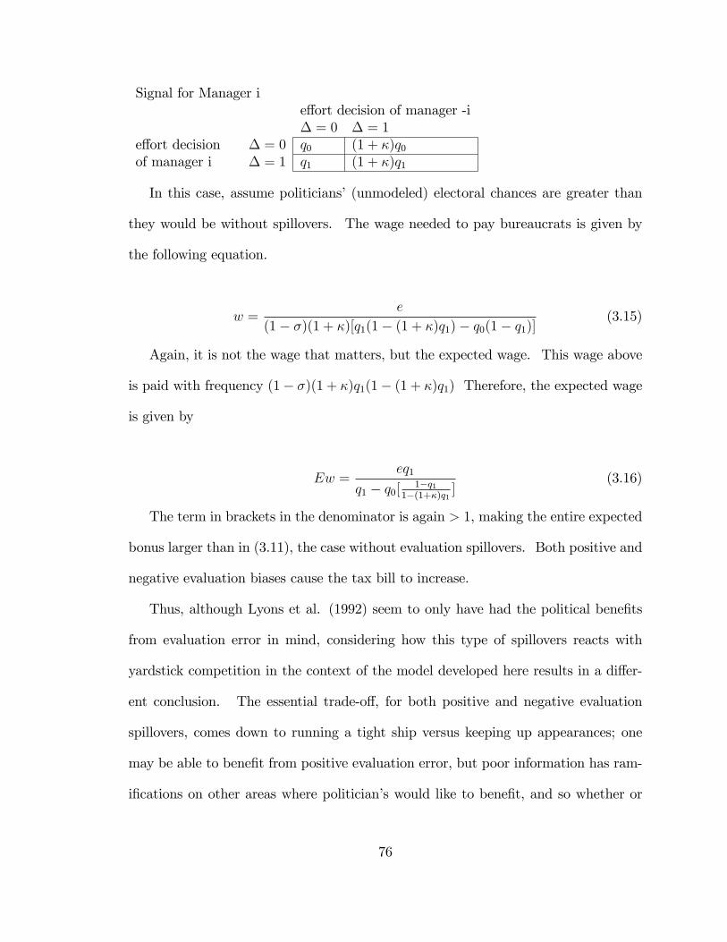
Signal for Manager ie¤ort decision of manager -i� = 0 � = 1

e¤ort decision � = 0 q0 (1 + �)q0of manager i � = 1 q1 (1 + �)q1

In this case, assume politicians�(unmodeled) electoral chances are greater than

they would be without spillovers. The wage needed to pay bureaucrats is given by

the following equation.

w =e

(1� �)(1 + �)[q1(1� (1 + �)q1)� q0(1� q1)](3.15)

Again, it is not the wage that matters, but the expected wage. This wage above

is paid with frequency (1� �)(1 + �)q1(1� (1 + �)q1) Therefore, the expected wage

is given by

Ew =eq1

q1 � q0[ 1�q11�(1+�)q1 ]

(3.16)

The term in brackets in the denominator is again > 1, making the entire expected

bonus larger than in (3.11), the case without evaluation spillovers. Both positive and

negative evaluation biases cause the tax bill to increase.

Thus, although Lyons et al. (1992) seem to only have had the political bene�ts

from evaluation error in mind, considering how this type of spillovers reacts with

yardstick competition in the context of the model developed here results in a di¤er-

ent conclusion. The essential trade-o¤, for both positive and negative evaluation

spillovers, comes down to running a tight ship versus keeping up appearances; one

may be able to bene�t from positive evaluation error, but poor information has ram-

i�cations on other areas where politician�s would like to bene�t, and so whether or

76

not evaluation error is good for a politician depends on the relative magnitude of each

trade-o¤.

3.4 Conclusion

This chapter has shown how mathematical translations of two prominent theories

are complementary to each other rather than substitutes. On what has been inter-

preted as their essence by several prominent authors, these theories are shown to be

orthogonal on a basic level. However the objective function and production function

are naturally connected, and a nested model is put forth as superior mathematical

translations of Oates (1972) and Williamson (1975). An extension explored an im-

plication of the political economy literature for corporate strategy; in particular, if

public good spillovers are present, they could lead to evaluation error, especially in a

political context where citizens are often asked about their satisfaction of city services.

Pursuing this idea showed that some intuitive reasoning can fail without taking into

account the factors associated with more complex models of optimal decentralization.

3.5 References

1. Alesina, A. and Spolaore, E, 1997. On the number and size of nations. Quarterly

Journal of Economics, 112, 1027-1056

2. Besley, T. and Case, A., 1995. Incumbent behavior: vote-seeking, tax-setting,

and yardstick competition. The American Economic Review, 85, 25-45

3. Besley, T. and Coate, S., 2003. Centralized versus decentralized provision of

local public goods: a political economy approach. Journal of Public Economics

77

4. Bryce, J., 1893. The American Commonwealth. London: Macmillan [�rst

published in 1888].

5. Calabrese, S., Epple, D., and Romano, R., 2007. On the political economy of

zoning. Journal of Public Economics, 91, 25-49

6. Che and Yoo, 2001. Optimal incentives in teams. American Economic Review

7. Kreps, D.M., 1996. Markets and hierarchies and (mathematical) economic the-

ory.�Industrial and Corporate Change, 5 p. 561.

8. Lyons, W. Lowery, D. and De Hogg, R., 1992. The Politics of Dissatisfaction:

Citizens, Services, and Urban Institutions. M.E. Sharpe.

9. Maskin, Qian and Xu, 2000. Incentives, information and organizational form.

Review of Economic Studies

10. Mookherjee, D., 2006. Decentralization, hierarchies, and incentives: a mecha-

nism design perspective. Journal of Economic Literature. 44, p367-390

11. Oates, W., 1972. Fiscal Federalism Harcourt Brace Jovanovich New York

12. Oates, W., 2005. Toward a second-generation theory of �scal federalism. Inter-

national Tax and Public Finance, 12, 349�373

13. Quin, Y. and Xu, C., 1993. Why China�s economic reforms di¤er: the M-form

hierarchy and entry/expansion of the non-state sector. Economics of Transition,

1, 135-170

14. Quin, Y. Roland, G. and Xu, C., 2005. Coordination and experimentation in

M-form and U-form organizations. mimeo

78

15. Quin, Y. Roland, G. and Xu, C. (2006) Coordination and experimentation in

M-form and U-form organizations. Journal of Political Economy

16. Sargent, T. 1993. Bounded Rationality Macroeconomics. Oxford: Clarendon.

17. Selton, R. 2001. What is bounded rationality? in Bounded Rationality: The

Adaptive Toolbox by Gerd Gigerenzer, Reinhard Selten, eds. MIT Press

18. Simon, H., 1957. Models of Man. New York: Wiley.

19. Spulber, D., 2007. Global Competitive Strategy. Cambridge University Press.

20. Vihanto, M., 1992. Competition between local governments as a discovery

procedure. Journal of Institutional and Theoretical Economics, 148, p. 411

21. Williamson, O., 1975. Markets and Hierarchies Free Press

3.6 Appendix

3.6.1 Background

This section aims to describe the essence of the M-form/U-form corporate form,

and federal/centralized governance distinctions, and to put the distinctions in some

historical perspective.

As an example of a transformation fromU toM-form: FordMotor Company before

WorldWar I was organized along functional lines and produced only a small number of

product lines, but today is composed of a number of relatively self-contained divisions,

including its Ford brand, as well as Lincoln, Land Rover, and several others. Each

product line division has their own functional division and so can be thought of as

a "scaled down U-form", which is a relatively autonomous pro�t center within the

79

larger Ford Motor Company. This is di¤erent from a holding company, because while

the divisions are di¤erent businesses, they are related.

In the left hand side of �gure1, the hierarchical structure of a multi-function,

multi-product, functionally organized �rm appears with a CEO at the top of the

hierarchy, to whom two middle managers report. These middle managers, connected

to the CEO, are F1 and F2 (for function 1 and function 2, which can be, for example,

the functions �nance and marketing, respectively). Each middle manager in turn has

two lower level employees working under them. This is to say, both product lines P1

and P2 have two individuals that report to each middle manager. The product-based

�rm, on the right hand side of �gure 3.1, also has a CEO at the top, but now the

middle managers are P1 and P2, and each oversees their own functional workers.

Turning to the political realm, a prototypical example of a federal government is

the United States. In �gure 3.2, governments appear as a multi-layered and frosted

cake. A centralized government, depicted on the left-hand side of �gure 3.2, is sliced

through the center, dividing the cake horizontally by layer. Each layer represents a

function, such as police, �re or ambulances. Federal governments, rather, are sliced

in the usual way of cutting a cake; that is, straight down from top to bottom. One

cannot see the individual layers, which are the functions these governments provide,

until the pieces are moved apart. However it is clear which government is responsible

for providing these functions to the given areas (or "jurisdictions") of the cake.

80

Figure 3.1 The basic U-form/M-form distinction in a multiproduct, multifunction �rm

Figure 3.2 Centralized versus Federal political structure

3.6.2 Derivation of expected bonus

This section shows how to derive the size of the bonuses the city must pay manager to

elicit e¤ort, using the framework of Che and Yoo (2001).

81

Under a centralized regime, the city has two options: pay the one manager a bonus only

when the signal is good or only when it is bad. It is easy to show the latter option is not

optimal. Minimization of the bonus goes on under the constraint that

[� + (1� �)q1]w � e � [� + (1� �)q0]w (3.17)

This is an incentive compatibility constraint.

Minimization implies that this constraint holds with equality, thus deriving the equation

number (3).

Under a decentralized regime, the city can make each of the two manager�s bonuses

depend on the signal of both. This is optimal, because the signal of the other contains

information about the other. In this case, minimization under the constraint

(1� �)q1(1� q1)w � e � (1� �)q0(1� q1)w (3.18)

And solving this as an equality results in the equation number (2). While the wage

paid under a centralized regime is lower than the bonus paid in a decentralized regime, the

former is paid more often than the later. Thus the city�s expected wage bill from paying

bonuses is equal to

e(1��)(1�q1)(q1�q0)(1� �)q1(1� q1) =

eq1(q1�q0) (3.19)

under a decentralized regime, and

e(1��)(q1�q0)(� + (1� �)q1) =

e�(1��)(q1�q0)+

eq1(q1�q0) (3.20)

82

under a centralized regime. Thus the cost of a bonus in a centralized regime is always

greater whenever � > 0; that is, whenever there is a common component to the signal.

In the case of an evaluation spillover, the only change in solving for the expected bonuses

comes from the probabilities.

3.6.3 Spillovers in the performance signals: part III

Other cases to consider are jealousy and pride. First the pride case; residents are overly

positive if their service is better than the other districts, and this has nothing to do with

the actual level provided. Rather than a mental error, these biases come about due to

citizen�s behavioral characteristics.

Signal for Manager ie¤ort decision of manager -i� = 0 � = 1

e¤ort decision � = 0 (1 + �)q0 q0of manager i � = 1 (1 + �)q1 q1

In this and the next case residents are not confusing anything but evaluation error is

still a¤ecting their judgement. With these types of spillovers, the bonus will actually be

cheaper to provide. The wage that will be paid to a worker in this case is:

w =e

(1� �)[q1(1� q1)� q0(1� (1 + �)q1)](3.21)

This is paid with frequency (1� �)q1(1� q1): Thus the expected wage is:

Ew =eq1

q1 � q0[1�(1+�)q11�q1 ]

As the term in brackets in the denominator is less than one, the overall expected bonus

is lower compared to the case without evaluation spillovers. Thus, pride makes yardstick

competition less expensive.

83

3.6.4 Spillovers in the performance signals: part IV

The fourth and �nal case is jealousy. Here, people are overly negative towards the

evaluation of their city�s services if the other district also has high quality service:

Signal for Manager ie¤ort decision of manager -i� = 0 � = 1

e¤ort decision � = 0 q0 (1� �)q0of manager i � = 1 q1 (1� �)q1

The wage that will be paid to a worker in this case is:

w =e

(1� �)(1� �)[q1(1� (1� �)q1)� q0(1� q1)](3.22)

The expected bonus is:

Ew =eq1

q1 � q0[ 1�q1(1�(1��)q1) ]

As before, the term in brackets in the denominator is less than one, and the overall

expected bonus is lower compared to the case without evaluation spillovers. Thus, jealousy

also makes yardstick competition less expensive.

84

CHAPTER 4

DISSATISFACTION AND TURNOUT: EVIDENCE FROMCITIZEN SATISFACTION SURVEYS

This paper explores the link between voter turnout and satisfaction. The problem

of explaining voter turnout has vexed social scientists for decades; on a theoretical

level, the failure to provide a convincing theory of voting has been put forth as one

of the main indictments of rational choice theory (Green and Shapiro, 1994). On an

empirical level, Matsusaka and Palda (1999) explain how, although many variables

have been found to be signi�cant determinants of turnout, the combined explanatory

power of all these variables remains low. However, few scholars have incorporated

satisfaction in their empirical speci�cations, and neither is it well integrated with

theoretical models of turnout.

At �rst pass, the manner by which dissatisfaction a¤ects turnout is a basic question

to which there are two intuitively pleasing, yet opposing hypotheses: dissatis�ed

citizens may become motivated, in what the literature has called negative voting,

making turnout more likely. On the other hand, dissatis�ed residents may become

apathetic, or alienated, making turnout less likely. Much of the literature on trust

and turnout in political sociology and psychology has expanded on these intuitive

85

hypotheses, and these arguments seem to be relevant in explaining the relationship

between satisfaction and turnout as well.

Upon deeper re�ection, it is plausible that both the forces of negative voting

and alienation are at play, and a useful theory of satisfaction and turnout must

thus account for the speci�c circumstances that dictate when each respective force

dominates. In this vein, the present study explores two ways to account for some of

these contextual factors. The �rst factor concerns how homeowners and renters may

react di¤erently in the face of dissatisfaction, and the second concerns previous voters

versus previous abstainers.

The classic book Exit, Voice and Loyalty by Albert O. Hirschman (1970) posits

two responses of dissatis�ed people - exit and voice.50 Which response a dissatis�ed

person uses depends on their level of loyalty, with loyal people being less likely to exit

and more likely to use voice. By this logic, homeowners who are dissatis�ed should

be more prone to participate in elections than renters, or at least, should not be as

likely to become alienated. This idea is developed below, and tested in the empirical

section.51 ;52

50This famous work is a classic example of integrating economic and political insights, keepingwith the organizational-political methodological approach of the �rst two essays. Exit from anorganization is the classic response of a dissatis�ed customer in the realm of the market, while voiceis by nature political.

51Although not formally stated in William A. Fischel�s The Homevoter Hypothesis, one implicationof homeowners being more responsive to local politics - as outcomes in this area a¤ect the value oftheir single biggest asset - would seem to be consistent with this notion, and thus a broader part ofFischel�s general theory.

52With respect to later development of the exit, voice and loyalty model, Lyons et al. (1992) rede-�ne loyalty as a response, and add a fourth, neglect, thus describing four responses to dissatisfaction,which vary along active-passive and constructive-destructive dimensions. Hirschman�s concept ofloyalty as a response determinant survives in what they call "investment"; "prior satisfaction" withthe organization and quality of "alternative" relationships are two other response determinants (seeLyons et al., 1992, pp. 56-57.)

86

The second method of taking contextual factors into account to determine whether

negative voting or alienation dominates, relies on the implications of learning-based

theories of voting (Kanazawa, 2000; Bendor et al., 2003). In these models, citizens

make decisions based on the outcomes from previous behavior. In its simplest form,

the main implication of these models is that dissatis�ed citizens who voted last time

should be less likely to vote next time and, the other side of the coin, that dissat-

is�ed citizens who abstained last time should be more likely to vote next time. As

such, these models incorporate aspects of both the negative voter hypothesis and the

alienation hypothesis; in particular, negative voting applies in the context of previous

abstainers, and alienation applies in the context of previous voters.

Data for the current study come from the National Citizen Survey, conducted

by The National Research Center (NRC). The NRC surveys citizens on satisfaction

with public services provided by local governments. Their survey instrument includes

questions on a variety of demographic and socioeconomic dimensions, including home

ownership, and whether the respondent voted in the last election, and plans to vote

in the next one.

Among the results of the empirical section are that the level of dissatisfaction

and turnout are negatively correlated for all residents, lending support to an "alien-

ation/reward" hypothesis, and rejecting the "negative voter/contentment" hypoth-

esis.53 This result is robust to the inclusion of income, race, age other control

variables.

53Although so far in this introduction the two main hypotheses have only been described in termsof alienation and negative voting, to be more precise, duty and contentment are also associated withthe each of the two main hypotheses, respectively.

87

The second is that the negative voter hypothesis is weaker for homeowners than

renters, contrary to homeowning�s implications for loyalty and concern for investment.

In fact, the estimated marginal e¤ect of dissatisfaction is negative for homeowners,

while for renters it is not statistically signi�cant. That is, the marginal e¤ect of

dissatisfaction on turnout for homeowners is not larger than for renters.

The �nal major �nding is a lack of support for the behavioral model of turnout, at

least as it pertains to abstainers.54 That is to say, dissatisfaction does not appear to

teach nonvoters to vote, as the learning hypothesis suggests. Instead, previous voters

who are dissatis�ed are less likely to vote, not more likely. Although theoretically the

behavioral model has logical appeal, and is able to generate plausible levels of turnout

(in contrast to past attempts, which have resulted in a "paradox of voting"55), the

data do not support the mechanisms by which turnout should be achieved. This

study does �nd that dissatis�ed voters do "learn" to stop voting, but this is a slight

bit of encouragement for the learning hypothesis.

Taken together, these results cast doubt on the negative voting hypothesis. Even

after accounting for contextual variables such as homeownership and previous voting

behavior, this hypothesis is consistently rejected by the data.

The next section reviews the voting participation literature, including the public

administration and socio-psychological branches. Through incorporating insights

from these literatures with the calculus of voting model, this section puts forth a

number of testable hypotheses regarding the relationship between dissatisfaction and

54However failure to reject both parts of the behavioral hypothesis is impossible, as the hypothesiscontains both of the main hypotheses.

55For reviews of the paradox, see Aldrich (1997) and Fedderson (2004).

88

turnout. The results of testing these hypotheses are presented in section three, and

section four summarizes the �ndings.

4.1 Theoretical Background

The e¤ect of dissatisfaction on turnout is part of a broader framework related

to the performance of government. Van Ryzin (2006, p.12), a public administra-

tion scholar, presents a useful framework for understanding the process by which

the performance of government ultimately a¤ects political behavior such as voting.

However, the public administration literature has not focused signi�cant attention on

voting in particular, and has rather discussed voice in general. When this literature

has dealt with speci�c voice responses, complaining seems to have been of primary

concern. Other branches of social science focus on voting participation, but these lit-

eratures use separate vocabularies, making it di¢ cult to integrate ideas from di¤erent

disciplines.

In Van Ryzin�s framework, the managerial strategy of public o¢ cials a¤ects service

outcomes, and these actual service outcomes, in turn, a¤ect the perceived outcomes

by the public. Perceived outcomes next determine a citizen�s level of satisfaction,

which then determines which response the citizen chooses. Of particular importance

for the present paper is when the citizen chooses voting. This last connection in the

Van Ryzin framework is of primary interest here. It,

...suggests a link between overall citizen satisfaction and trust of gov-ernment as well as other behavioral consequences, such as complaining orleaving a jurisdiction. These key behavioral consequences of dissatisfac-tion were put forth by Lyons, Lowery and DeHoog (1992) in what theyterm the EVLN model: exit: (leaving a jurisdiction), voice (complaining),loyalty (trust), and neglect (apathy or alienation)." (p. 8)56

56Lyons et al. (p. 55), who Van Ryzin cites, de�ne four responses:

89

While public administration scholars, political scientists, sociologists and psy-

chologists all talk about trust, satisfaction and turnout,57 the literature is so vast and

inconsistent in its use of these terms that it is essential to develop a common language

before proceeding. The main distinction can be put simply: the public administration

literature (e.g., Van Ryzin, 2006, and Lyons et al., 1992) conceive of satisfaction as

a¤ecting both exit and neglect, as well as trust (what they term loyalty) and voice,

the latter two of which are represented by arrows d and b respectively, in �gure 1 be-

low. Voting is associated with the "voice" response; thus satisfaction re�ects voting

through arrow b.58

Exit involves ending the relationship between the citizen and the local government.

This may take its most general form in the citizen�s leaving or intending to leave one

jurisdiction and moving to another� the classic Tiebout response.

"Voice" is probably the broadest and most familiar response category. If we con-

ceptualize voice as active and constructive e¤orts to improve conditions giving rise to

dissatisfaction, then much of what traditionally falls under the topic of political partici-

pation can be identi�ed as "voice"...

"Loyalty" entails passively but optimistically waiting for conditions to improve...This

very closely resembles the interpretation of the voting act and regime-supportive atti-

tudes found in the political participation literature.

"Neglect" is perhaps the most di¢ cult of the responses to de�ne...while such concepts

as disa¤ection, alienation, cynicism, and distrust have a long history in the general

political participation literature...apathy, nonvoting...are rarely viewed as responses to

speci�c sources of dissatisfaction...we are compelled to view neglect as something more,

given our focus on participation as responses to dissatisfaction.

57In their review of "Political Trust and Trustworthiness," Levi and Stoker (2000, p. 476) write,"...trust is a contested term..."

58To confuse matters further, Lyons et al. (1992) also associate voting with the "loyalty" response.They write, "Of course, it isn�t always intuitively obvious that a speci�c behavior falls into anyparticular or even only one of the four categories." However, to the degree that voting is an active,not a passive response, voting should be primarily associated with the voice category.

90

On the other hand, the socio-psychological literature has focused a great deal of

attention on how trust a¤ects voting (voice). Thus, "...scholars inspired to con-

sider the consequences of trust/distrust...for political participation have generated a

profusion of complex hypotheses." (Levi and Stoker, p. 488). The "trust in gov-

ernment" questions59 in the National Election Studies (NES) were "designed to tap

the basic evaluative orientations towards the national government." (Stokes, 1962, p.

64) Stokes�work, and the social unrest of the 1960s, prompted a signi�cant amount

of research on political trust, exempli�ed by Gamson�s 1968 Power and Discontent,

which featured trust as a central concept. All of this can be associated with arrow e

below.

Figure 4.1: Satisfaction a¤ects four responses; loyalty a¤ects voice

59Examples include, "How much of the time do you think you can trust the government in Wash-ington to do what is right�just about always, most of the time, or only some of the time?" and,"Would you say the government is pretty much run by a few big interests looking out for themselvesor that it is run for the bene�t of all the people?" As mentioned in a previous footnote, some ofthese questions may actually be measuring satisfaction.

91

One way to resolve this inconsistency is simply to assert that what the socio-

psychological literature has termed "trust" is often similar enough in de�nition to

what the public administration literature has called "satisfaction" to use them as

synonyms;60 that is, the two literatures simply use a di¤erent vocabulary, and �gure

1 does not represent the organizing framework that political scientists use. However

to say that when socio-psychological literature says "trust" they simply mean "satis-

faction" obscures the fact that the socio-psychological literature has indeed recognized

that trust measures are in�uenced by evaluations of the performance and policies put

in place by the incumbent government. (Levi and Stoker, 480). This suggests �gure

1 is indeed the framework socio-psychological scholars have in mind; they recognize

arrow d, but simply focus on arrow e.

Either method of resolving this inconsistency between the social science literatures

seems suitable for the purposes of the discussion here. Replacing the word "trust" in

the socio-psychological literature with "satisfaction" is the simplest method, although

it misses some of the intricacies of the theory. Doing this, however, means that the

socio-psychological explanations for how trust in�uences turnout are also relevant for

explaining how satisfaction in�uences turnout. Taking the second way out is on

some level just as simple a solution; satisfaction in�uences trust, and trust in turn

in�uences turnout.

60Consider the following survey question, taken by many to be a measure of trust, "Do you thinkthat people in the government waste a lot of money we pay in taxes, waste some of it, or don�t wastevery much of it?" While this may be consistent with de�nitions of trust, it is also consistent withde�nitions of satisfaction. Thus, much of the data used to test the relationship between trust andturnout is in fact measuring satisfaction and turnout. As a �nal case in point, when Besley (2006)talks about "satisfaction with government" and "whether turnout and declining voter satisfactionwith politics and politicians are linked," it is in the subsection entitled "Trust and turnout."

92

Recognizing the di¢ culty in integrating insights from all of these literatures paves

the way for a more formal discussion, into which the insights from the informal lit-

eratures can be incorporated. To frame the voting decision, this study employs

the calculus of voting model (Anthony Downs, 1957; Gordon Tullock, 1967; William

Riker and Peter Ordeshook, 1968). This classic model is a decision theoretic setup

that de�nes the bene�ts of voting as pB + d where p is the exogenous probability of

being decisive in the election, B is the net expected utility from the realization of the

preferred outcome, and d is the bene�t a citizen feels from doing his civic "duty".

The calculus of voting model conceives voters as rational actors who maximize

subjective utility. A citizen votes if the bene�ts, pB + d, exceed the cost of voting,

denoted c. The costs of voting include both the "costs of registering and going to

the polls," and "information costs associated with determining B." (Moon, 1992, p.

127) In most cases (i.e. reasonably large elections) the probability of being decisive,

p, will be trivial, and the decision to vote comes down to a comparison of c and d.

How could satisfaction (or trust) a¤ect turnout in this model? Timothy Besley

(2006, p. 17) has suggested that the link between satisfaction and turnout could be

understood through the d term in the calculus of voting model:61

...political scientists tend to work in frameworks where some extra com-ponent of utility (such as social duty) is invoked to explain why people

61In his extension, Moon (1992) breaks down the d term into three theoretically meaningfulcategories:1. a sense of satisfaction derived from discharging one�s "duty," induced by socialization and

altruism,2. a sense of satisfaction derived from exercising one�s prerogatives, induced by e¢ cacy,3. a sense of solidarity conferred by groups one feels connected with; social rewards.Satisfaction with government performance could conceivably enter through each of these three

channels. The typical notion of the word "duty" is re�ected in the �rst component of the d term,denoted d1. Besley (2006) seems to have in mind that satisfaction a¤ects d through the d1 route.However, it also seems reasonable if an e¢ cacious person who is dissatis�ed receives bene�ts from d2,and a satis�ed person who may enjoy seeing their dissatis�ed neighbors at the polls (schadenfreude),bene�ts through d3.

93

vote in such large numbers. In this case, election turnout could be abarometer for how such feelings of duty extend in the population. To theextent that [feelings of social duty] are correlated with perceived satisfac-tion with government, this could create a link between turnout and thequality of government...62

Here Besley suggests the mechanism by which satisfaction a¤ects turnout: d =

d(satisfaction). However he does not answer the question how (in which direc-

tion) it a¤ects turnout.

One possibility is that dissatisfaction and turnout are negatively correlated, which

is to say satisfaction and turnout are positively correlated. In this case, voters who

are happy with public service reward public o¢ cials for providing good performance,

or provide public goods/contribute to the collective action (voting). This could also

come about if dissatis�ed citizens choose the "neglect" response, and not the "loyalty"

response; the concept of alienation indeed goes back very far in the social sciences

(see Seeman, 1959, for an early discussion of alienation and attempt to clarify its

meaning). Levi and Stoker (p. 486) discuss how alienation has long been associated

with a response of distrust:

The idea that distrust might discourage political engagement was in-spired by early theorizing about satisfaction and alienation (Stokes 1962,Almond and Verba 1963, Finifter 1970) and by the fact that the over-timedecline in US voting turnout coincided with the over-time decline in trustin government.

If dissatisfaction is related to the d-term, as Besley (2006) suggests, and if dissat-

isfaction leads to alienation, and/or satisfaction leads to loyalty, this is all consistent

with the following hypothesis:

62Besley goes on to say, "...but the link is tenuous at best. If social duty is the main basis ofdeciding to vote, then declining turnout could also be linked to a general decline in �social capital�,i.e. a willingness by citizens to privately provide public goods." This comment suggests there areproblems with empirical time series analysis of voting and trust or satisfaction; the cross-sectionalapproach of the next section mitigates these concerns.

94

Hypothesis 1:@d

@�< 0

Where � denotes dissatisfaction. Hypothesis 1 could come about either because

dissatis�ed people become alienated, or if satis�ed people contribute to collective

action. Hypothesis 1 thus posits how the alienation/duty theorem of participation

�ts into the calculus of voting model. The decision to represent the evaluation of

government as dissatisfaction �; rather than satisfaction, say with �; is arbitrary.

The negative derivative can be due to either duty, alienation, or both; duty and

alienation are not mutually exclusive, and can both be the explanation for the negative

derivative in hypothesis 1.63

Having chosen d as the channel by which satisfaction a¤ects turnout in the calculus

of voting model, how else could satisfaction a¤ect turnout? The political psychology

and sociology literature is again informative here. Levi and Stoker (2000) also explain

the rational for negative voting. If one replaces "trust" everywhere below with

"satisfaction," the rationale for negative voting as a force in political participation is

that:

...distrust, not trust, should stimulate political involvement� or at least,distrust should stimulate political involvement among those who feel polit-ically e¢ cacious. This claim was articulated �rst by Gamson (1968, 1975),a political sociologist, and in a complementary way by Bandura (1982), apsychologist. In an often-cited passage, Gamson (1968:48) stated that "a

63It should also be noted that choosing to focus on how satisfaction a¤ects the d term is alsoarbitrary. For example, others have focused on the pB term to understand turnout. The turnoutmodel of Thomas Palfrey and Howard Rosenthal (1983) endogenizes the probability that a voterwill be pivotal. However as these authors note, p is su¢ ciently small in any large election so thatturnout again is e¤ectively a function of d being larger than c. The paradox of voting - where peoplevote despite their low probability of being decisive - is still present in the absence of the d term.

95

combination of high political e¢ cacy and low political trust is the opti-mum combination for mobilization� a belief that in�uence is both possibleand necessary."

The main point is, if people are e¢ cacious, then distrust, or dissatisfaction, should

strongly encourage voting.64 Negative voting has a long history in social science, as

Radcli¤ (1994) points out:

The classical voting behavior literature is replete with suggestions of neg-ative voting. In the two best-known examples, Key (1966) posits that"people vote only against, never for," while Campbell et al. (1960) con-jecture that the electorate "is more likely to punish an incumbent partyfor its mistakes than reward it for its successes."

In addition to its long history in the literature, negative voting also makes intuitive

sense: satis�ed people become complacent, or content, and will not act unless some-

thing bad happens to shake them out of their complacency.

Hypothesis 2:@d

@�> 0

Just as there are two sides to hypothesis 1, alienation and duty, hypothesis 2

also contains two sides; here, abstention occurs through satisfaction, or contentment.

Therefore, hypothesis 2 posits the negative voting/contentment hypothesis.

Hypotheses 1 and 2 are the core competing hypotheses that will be put to the test

in the empirical section. Two related hypotheses, to be discussed below, attempt to

deepen the theory of satisfaction and turnout. These two hypotheses both maintain

the following premise: both hypothesis 1 and 2 can be true, and a deeper theory

of turnout and satisfaction must account for when the forces behind each respective

64Looking ahead to the empirical section, citizens who �ll out satisfaction surveys would seem tobe individuals with a higher than average level of e¢ cacy.

96

hypothesis dominate. This is to say, the derivative of d with respect to � may some-

times be positive, and sometimes be negative, and the magnitude of this derivative

will vary in predictable ways.

The �rst of these hypothesis comes from the �eld of psychology. As Dennis

Mueller (1999, p. 325) notes:

Behavioral psychology o¤ers a relatively simple description of the learn-ing process...Actions followed by rewards increase in frequency. Actionsfollowed by punishment decline in frequency. Man learns to avoid doingthat which brings about pain, and to do that which produces pleasure.

A representative paper in this approach, Kanazawa (2000), posits that this notion

can be captured through the d-term in the calculus of voting model.65 To illustrate

hypothesis 3 by modifying his framework, imagine dt+1 = dt+([dtv]� [dt(1� v)]),

where di is the level of feelings of "duty" in period i, v = 1 if the individual voted in

the election between period t and t+1, and 0 if not; = if � = 0; and = � if

� = 1.66 "...captures the magnitude of reinforcement or punishment in the learning

process." (p. 436) In this setup, voters "...do not perceive the causal link between

their contribution and the collective action outcome, but merely the correlational

links." (p. 435)67

Denoting a voter who did not vote in the last election as a (for abstainer), and

a voter who did vote in the last election as v (for voter), the learning hypothesis of

satisfaction and turnout, framed in the calculus of voting model, can be stated as

follows:

65He also posits that the behavioral mechanisms can be captured through the P term as well asthe d-term. In his model, there is a lag in reinforcement when it a¤ects non-instrumental utility.

66In his framework, � represents the preferred outcome did not occur in period t.

67This setup can also be used to illustrate negative voting and alienation; for negative voting,dt+1 = dt + [dt], and for alienation dt+1 = dt � [dt]:

97

Hypothesis 3:@dv

@�< 0 <

@da

@�

Hypothesis 3 is a sample composition e¤ect; one part of the population behaves dif-

ferently from another. It contains elements of both the negative voting/contentment

hypothesis and the alienation/duty hypothesis, and uses previous electoral behavior

to di¤erentiate between the two. In this framework, two groups of people are more

likely to vote, compared to their previous participation level: dissatis�ed nonvoters

and satis�ed voters. The two groups that are less likely to vote are dissatis�ed

voters and satis�ed abstainers. In a nutshell, hypothesis 3 says that the negative

voter/contentment hypothesis holds for abstainers, and the alienation/duty model

holds for voters.

The second hypothesis that distinguishes between the two main hypotheses is also

a sample composition e¤ect, and rests on behavioral di¤erences between homeowners

and renters. The "homevoter" hypothesis (Fischel, 2001) begins with the premise

that homeowners take purposive action to maximize their home value. From this it

follows that homeowners are more likely to vote than renters. However it also implies

something more subtle: if homeowners are dissatis�ed with government service, they

have a stronger incentive to make their voice heard (and one way to do this is through

voting), than renters. This higher likelihood of voting in the face of dissatisfaction is

in addition to the general propensity of homeowners to vote at higher rates. Fischel

(pp. 30-31) writes:"...because poor municipal service adversely a¤ects the value of

their homes, homeowners have strong reasons to bring it to the attention of their

elected o¢ cials..." This implies that dissatis�ed homeowners are more likely to vote.

98

This suggests negative voting, not alienation, should be more likely to be present

among home owners. This is not to say that negative voting could not be present

among renters, but renters, lacking such investment in the community, do not have

the same pressures preventing them from becoming alienated as face homeowners.

Moreover, renters have another option that is less feasible for homeowners; dissatis�ed

renters can exit the jurisdiction.

Lyons et al. (p. 56) discuss this general point:

Citizens who are highly invested in a particular jurisdiction are morelikely to adopt constructive behaviors since they have more to lose thanpoorly invested individuals who would be expected to respond by eitherallowing the situation to decay further (neglect), or, alternatively, movingfrom the jurisdiction or privatizing the service that is the source of dissat-isfaction (exit). These investments can include such tangible investmentsas homeownership, employment, or children in the schools of the jurisdic-tion. They can also embrace social and psychological investments arisingfrom long-term residence in and attachment to the jurisdiction. In ei-ther case, jurisdiction-speci�c commitment arising from such investmentsshould increase the propensity of individuals to exercise voice or loyaltyin the face of dissatisfaction.

As we are conceiving voting as both a voice and loyalty response, this is all con-

sistent with hypothesis 4. None of this is inconsistent with the previous discussion of

negative voting, alienation, reward and contentment. However, it does suggest how

homeowners (more loyal citizens) may react di¤erently in the fact of dissatisfaction.

Formally, denoting homeowners by h and renters by r, the derivative of d with respect

to satisfaction should be smaller for homeowners than renters.

Hypothesis 4:@dh

@�>@dr

@�

While hypothesis 4 could arise just because homeowners are more likely to vote

than renters, the larger implication (which has not been articulated in the literature) is

99

that behavioral responses to dissatisfaction di¤er between these two types of citizens.

In an empirical context, this means controlling for homeownership, the relationship

between dissatisfaction and voting presented in hypothesis 4 still holds.

Hypothesis 4 is also a sample composition e¤ect. However, it does not divide the

sample into two distinct hypotheses, as did hypothesis 3. Hypothesis 4 can be con-

sistent with the negative voter hypothesis for both groups, the alienation hypothesis

for both groups, or the negative voter hypothesis for homeowners and the alienation

hypothesis for renters. What it does rules out is the negative voter hypothesis for

renters along with the alienation hypothesis for homeowners, and it provides for a

prediction on the magnitude of the derivative in all cases.68 ;69

4.2 Empirical Background and Methodology

This section uses the NRC data to estimate the following three empirical models:

votingi = b0 + b1dissati +BX + � (4.1)

votingi = b0 + b2(dissati � h-owneri) + b3(dissati � renteri) +BX + � (4.2)

votingi = b0 + b4(dissati � votedi) + b5(dissati � abstainedi) +BX + � (4.3)

68The formal framework can also incorporate hypothesis 4. In this case, dt+1 = dt + k([dt(1�h)]�[dth]).where h = 1 if the individual is a homeowner, and h = 0 if a renter, and k is a parameterthat can either be positive or negative, re�ecting the general response to dissatisfaction.

69The underlying logic behind Hypothesis 4 is that homeowners are more invested in the commu-nity than renters. Therefore, other ways of splitting the population, such as by number of yearsspent living in the community, would yield analogous predictions.

100

votingi is a dummy variable equal to one if the individual plans on voting in the

next election; dissati is equal to one if the individual is dissatis�ed with government

performance;70 h-owner is equal to one if the individual is a home owner, and

renteri is equal to one if not; votedi is equal to one if the individual voted in

the last election, and abstainedi is equal to one if not.71 The vector X contains

standard socioeconomic control variables, described below, plus h-owner, votedi

and registered, a dummy equal to one if the individual is registered to vote.

Recasting the theoretical discussion of the previous section in terms of the em-

pirical models in (4.1)-(4.3): the alienation/dutiful voter hypothesis (Hypothesis 1)

predicts a negative coe¢ cient on b1: The negative voter/contentment hypothesis

(Hypothesis 2) predicts a positive coe¢ cient on b1. The homevoter hypothesis (Hy-

pothesis 4) and learning hypothesis (Hypothesis 3) add complexity and recognition of

the fact that both forces could be at play; these suggest that b2 > b3 and b5 > 0 > b4,

respectively. This section aims at testing these four hypotheses, as well as providing

a benchmark measure of the importance of dissatisfaction in explaining turnout.

Before turning to the data, a brief review of related studies places this study

in context. Although previous studies have not used citizen satisfaction data to

explore the determinants of turnout, the present study relates to a vast body of

research. Mueller (2003) and Geys (2006) describe numerous empirical studies of

turnout. Taken together, the studies they review identify several variables that have

70As will be discussed, measures of this variable are from the city, state and federal levels; theseare denoted citydissat, statedissat, and feddissat, respectively.

71As equations (4.1)-(4.3) suggest, the variables described in the text are used to construct avariety of interaction variables. In particular, interactdh is an individual that is both dissatis�edand a homeowner; interactdr is an individual that is both dissatis�ed and a renter; interactdvis an individual that both is dissatis�ed and voted in the last election; interactda is an individualthat both is dissatis�ed and abstained in the last election.

101

generally been found to be signi�cant, including population size and closeness of the

election. Both of these are related to the probability of being decisive, and are

thus critical in the calculus of voting model. Unfortunately, these variables are not

available in the NRC data.

The literature Mueller (2003) and Geys (2006) review for the most part do not

focus on variables such as age, income, race, sex, education level, and tenure (home-

ownership) status of the citizen. These variables have usually been included in

empirical speci�cations as "control variables" and have often been shown to be sta-

tistically signi�cant. The standard expected relationship is that older, richer, white,

educated homeowners should be more likely to vote. These expectations presumably

arise in these studies due to "conventional wisdom." However, there is a branch of

the social science literature that provides microfoundations for why these variables

determine turnout. The "resources model of participation" (Verba and Nie, 1972),

suggests that, "...the social status of an individual - his job, education, and income -

determines to a large extent how much he participates. (p. 13)

The present study follows Kanazawa (2000) by including age, race, sex, income

and education. The main focus here is on the variables constructed with measures

of dissatisfaction, and so like much of the literature, these e¤ects of the "control"

variables on turnout will not be the main focus of the discussion.

With respect to tests of the negative voter versus alienation hypotheses, Radcli¤

(1994) found negative empirical correlation between self reported economic changes

and turnout; that is, people who became worse o¤were less likely to vote, suggesting

that people who found themselves in a worse position became apathetic, or alienated,

102

rather than motivated to vote. However other studies have found the opposite. Ker-

nell (1977) argues that voters in post-WWII midterm elections who disapproved of

the president were more likely to vote than those who approved. In short, the issue is

not agreed on this literature (see the discussion in Radcli¤ for more references.) Simi-

lar divergent �ndings have been produced in the trust literature. The conjecture that

distrust discourages voting has been discon�rmed in a variety of studies (described

in Levi and Stoker, p. 486, n. 5) Besley (2006) however provides historical data to

show "suggestive evidence" that distrust does indeed discourage turnout. Thus the

trust literature, like the voting participation literature, is inconclusive.

Much less empirical work tests the learning model of turnout. Kanazawa (1998,

2000) �nds support, but Martin and Shieh (2003) review the data used in Kanazawa

(2000) and conclude that the �nding of support is merely due to coding error. With

respect for the homevoter hypothesis, Fischel (2001, p. 80 and elsewhere) discusses

how, "Nearly every study has shown that renters participate in local a¤airs in dispro-

portionately low numbers compared to homeowners." As mentioned above, his study

does not deal with the speci�c implication of the homevoter hypothesis of interest to

the present study. Some of the public administration literature is relevant here, how-

ever. Lyons et al. (1994, p. 73) �nd that dissatis�ed homeowners are signi�cantly

more likely to use voice behavior, although they did not use voting as a measure of

voice behavior.

To test among these competing hypotheses, this section uses the NRC data, which

provides multiple measures of satisfaction and turnout at the individual level. In ad-

dition, this data includes a variety of demographic and other measures that have been

shown to be signi�cant determinants of turnout in previous empirical studies. As of

103

this writing, the National Citizen Survey (NCS) had been conducted in 122 cities and

counties in 36 states. Surveys are mailed to citizens in these cities, and ask a variety

of questions related to satisfaction with city services. For their part, cities use results

from these surveys for program planning, budgeting, goal setting and performance

measurement. (http://n-r-c.org) The appendix contains a list of the 122 cities sur-

veyed, as well as a copy of the survey instrument. The data analyzed in this study is a

subset of the NCS database, containing 4,781 individual level observations from nine

communities,72 the identity of which was not disclosed to the author. After dropping

observations with missing values, responses from 3313 individuals remained.73

The variable voting comes from question 34: "Are you likely to vote in the next

election?" For the entire sample, 90.8% responded "yes" to this question. The

variable voted comes from question 35: "Did you vote in the last election?" 72.7%

of the sample responded "yes" to this question. Among people who said they voted

in the last election, almost all of them (99.5%) said they were likely to vote in the next

election. This �gure is extremely high, especially if respondents take the elections to

mean local elections, where turnout is generally lower.74 Although these questions

72NRC also provided the author with data from a tenth jurisdiction, however it did not containdata needed for the dependent variable, and so was dropped from the sample.

73Although many responses contained at least one missing observation, the regression resultsreported below were robust to the inclusion of as many omitted observations as possible; for example,some observations were dropped only because they did not contain statedissat, even though theseobservations could have been used in all the speci�cations reported in table 3.

74A theoretical explanation for the established empirical regularity of lower turnout in local elec-tions comes from Fischel (pp. 89-90):

Low political participation, however, could also be a sign of satisfaction by adult

residents who, in nearly all cases, deliberately chose to live in an particular town...Bill

Niskanan suggested to me, higher participation at the national level re�ects the lack

of "exit" options from that jurisdiction.

104

do not distinguish between types of elections, it is reasonable to assume respondents

had local elections in mind, given the surveys are primarily about satisfaction with

local government.

Among people who said they did not vote in the last election, 36.6% said they

were likely to vote in the next election. This seems like a more plausible �gure. Of

the 3,313 observations used in the analysis, the four types of voters, where (voted,

voting) is (1,1), (1,0), (0,1) and (0,0), represent 2584 (78%), 11 (.003%), 263 (8%),

and 455 (14%), respectively. Given the possibility that the people who say both

they voted in the last election and are voting in the next election are lying, a fourth

speci�cation is outlined below. If the results of speci�cation (4.4) are the same as

(4.2),the �ndings with respect to the homevoter hypothesis can be taken to be more

robust.

votingi = b0 + b6(dissati � abstaineri � h-owneri)

+b7(dissati � abstaineri � renteri) +BX + � (4.4)

A dummy variable interactdah is equal to one for an individual that is dissatis-

�ed, abstained, and is a homeowner, while the variable interactdar represents an

individual who is dissatis�ed, abstained and is a renter.75

A variety of respondent-speci�c controls come from the survey instrument�s ques-

tions. Unfortunately the actual jurisdiction is unknown, but population characteris-

tics can be inferred from sample statistics. Table 4.1 below summarizes population

75Many studies of turnout su¤er from the problem of over reporting, see for example Matsusakaand Palda (1999, pp. 433-434) and Kanazawa (2000, p. 439-440). Kanazawa employees a methodthat is in some ways similar to the approach taken here, while Matsusaka and Palda cite papersthat show, "evidence from vote validation studies that it is unlikely to have a material a¤ect (sic)on most research that makes use of survey data." (p. 434)

105

averages of a variety of respondent data for the nine jurisdictions. Although it ap-

pears that the nine jurisdictions are remarkably similar, at least in the case of the

variable age this is partially due to the speci�c method of coding the data.76

The main independent variable of interest, dissati, comes from question 11.

"Overall, how would you rate the quality of the services provided by the city/county of

ABC?" This question also asks about the respondent�s rating of the state and federal

governments; a rating of poor for the city, state and federal governments, respectively,

are denoted citydissat, statedissat, and feddissat. The basic statistics about

dissatisfaction with di¤erent levels of government are quite pronounced. People of

all income levels are more satis�ed with the performance of local government, than

either state and federal. In particular 4.8%, 13% and 11.7% of the sample rate

the performance of city, state and federal government as poor, respectively. These

statistics are consistent with �ndings in the trust literature, where people distrust

federal government more than local government. One explanation for this is that,

"...the tasks of local governments are easier to perform and to evaluate, and that

citizens �nd local government more responsive to their concerns..." (Levi and Stoker,

pp. 482-483).

76age is a categorical variable, but is expressed as an ordinal measure, using the median value ofin each response category.

106

Table 4.1: Sample population summary statistics, by jurisdiction

A more striking statistic comes from looking at dissatisfaction with di¤erent lev-

els of government among di¤erent income classes. The percentage of low income

people that are dissatis�ed with local, state and federal government, respectively, are

5.7, 17.7, and 13.8. Among high income people, the statistics are 3.2, 12.5, and

11.1. There are minor variations among these groups�perception of state and federal

government (high income perceive both slightly more favorably), but there is a big dif-

ference between how these groups perceive local government, with low income people

almost 80% more dissatis�ed with local government on average than high income.77

A theoretical explanation for these statistics comes from the model by Morelli, Yang

and Ye (2007, p. 1), which compares centralized systems of government (e.g. states)

77The lowest income level is 1.78 times more dissatis�ed with local government, 1.41 times moredissatis�ed with state government, and only 1.24 times more dissatis�ed with federal government.

107

versus decentralized systems (e.g. cities). They show that, "The rich should al-

ways be in favor of competing authorities and local governments..." The intuition

behind their result is that local level services are typically competitive, and typically

competition favors the high productivity and high income type.

Individual-level variable summary statistics for the entire sample are presented in

Table 4.2. Many of the variables that have not yet been de�ned are self explanatory:

age comes from question 30 and is coded as described in footnote 74. The rest of

the variables are dummy variables: nonblack comes from question 29; male from

question 31; eddegree from variable 26 (if the individual had an associate degree

or higher); lowinc from question 27. While there are no surprises, given the type

of survey from which the data come, it is interesting to note that about 57% of the

respondents were women. A large proportion are homeowners (78%), and almost 43%

have an educational degree. For the interaction variables, of dissatis�ed residents

71% (.0344/.0485) were homeowners, and 73% (.0353/.0485) were previous voters.

108

Table 4.2: Summary statistics for individual characteristics

Results from regressions on speci�cations (4.1)-(4.4) are reported in columns 1-4 in

Table 4.3 below. In the �rst column, the main estimate to note is the marginal e¤ect

on citydissati. In this speci�cation, the estimated marginal e¤ect is negative and

highly signi�cant. This �nding rejects the negative voter/contentment hypothesis,

and lends support for the reward/alienation hypothesis.78

78The speci�cations reported below were also tried with the dissatisfaction variable equal to oneif the respondent answered either fair or poor to q11a. Qualitatively similar results obtained whenusing these two de�nitions of dissatisfaction, and so to economize on space, this study only reportsresults using the de�nition of dissatisfaction described in the text. In addition, de�ning the variableas equal to one if the respondent indicated "excellent" does not qualitatively change results; ratherthan a negative marginal e¤ect, a positive marginal e¤ect arises. Including dummies for bothdissatisfaction and satisfaction at the same time results in only dissatisfaction being signi�cant.

109

The R2 in this speci�cation is .5746. The inclusion of citydissat only slightly

raises the R2; in a speci�cation identical to (4.1), except for the omission of citydis-

sati (such a speci�cation is reported in column 1 of table 4.4, in the appendix) the R2

was .5679. While including citydissat only raises the R2 by .0066, this adds more

than does any of the other variables in column 2, except voted and registered.

The signs and signi�cance of the control variables in this speci�cation are for the

most part as expected. voted and registered are both positive and signi�cant;

both are also of similar magnitude, between .15-.16 in all three speci�cations. Of the

socioeconomic and demographic variables, age is consistently signi�cant, however it

is negative, at odds with the �ndings of previous studies. Surprisingly, young voters,

at least those who respond to citizen satisfaction surveys, are more active voters than

other age groups who respond to these surveys. This suggests that while young

citizens in the population at large may be less politically involved, there may be a

small but especially active group among them.

All of the other control variables are of very small magnitude and in any case

are not signi�cant, with the exception of lowinc. This variable is negative, con-

sistent with the �ndings of previous literature. homeowner is not signi�cant in

this speci�cation.79 In later speci�cations, to be discussed, eddegree is marginally

signi�cant and positive, as expected, although it is not signi�cant in the speci�cations

reported in table 4.3. Other than the marginal e¤ect on eddegree, the rest of the

estimates do not di¤er much across the speci�cations.

79It seems that voted and registered take away the explanatory power of homeowner. Inspeci�cations without these two variables (not reported here) homeowner was positive and signif-icant, but its signi�cance fell to marginal after adding registered, and fell completely after thenadding voted.

110

Moving back to dissatisfaction, how do the results di¤er among homeowners ver-

sus renters? The answer is quite pronounced: in Table 4.3, column 2, dissatis�ed

homeowners are signi�cantly less likely to vote, as indicated by the negative marginal

e¤ect on interactdh, whereas there is no propensity among dissatis�ed renters to

either vote or abstain, as the estimated marginal e¤ect on interactrd is not signif-

icantly di¤erent from zero. The t-test that these marginal e¤ect are the same fails

(with chi2(1)=.78; prob>chi2=.3759). The size of the marginal e¤ect on interac-

thd is smaller (more negative) than it was in citydissat in the �rst speci�cation,

indicating that homeowners are more likely than the population as a whole to react

to dissatisfaction with alienation. This is counter to the homevoter hypothesis, be-

cause dissatis�ed homeowners should be more likely to vote than dissatis�ed renters,

whereas the data shows just the opposite: dissatis�ed homeowners are less likely to

vote, even while controlling for homeownership.80

The third speci�cation tests whether people who voted in the previous election

were more or less likely to respond to dissatisfaction by voting in the next election.

Results indicate both dissatis�ed previous voters and dissatis�ed previous abstain-

ers are less likely to vote in the next election, as indicated by the negative marginal

e¤ect on interactdv and interactad, respectively. The marginal e¤ect on in-

teractdv is smaller than interactad, suggesting the e¤ect of dissatisfaction on

turnout is larger for voters. The t-test that these marginal e¤ect are the same fails

80Using loyalty, a variable equal to one of the resident lived in the city for eleven years or more,results in di¤erent �ndings. Again, the estimated coe¢ cients on interactld and interactud areboth negative, the former -.0314** ( .021), the latter -.053*** (.033). Thus, the latter is smallerthan the former, as predicted by the theory. All the other variables do not vary substantially fromthose in speci�cation three. The variable loyalty, which contains 4724 observations, has a meanof .62 and standard deviation of .49. The variables interactld and interactud each have 4479observations, and means .0339361 and .0174146, respectively.

111

(with chi2(1)=2.19; prob>chi2=.1389). This overall �nding is inconsistent with of

the behavioral model of turnout (although the relative magnitude of the estimated

coe¢ cients is in line with what the behavioral model predicts.)

The �nal column in table 4.3 reports the marginal e¤ects of the variables in speci-

�cation (4.4). This speci�cation essentially aims at testing the homevoter hypothesis,

but only among renters and homeowners who indicated that they abstained in the

previous election. The results are similar to those from column 2: dissatis�ed home-

owners are less likely to vote, whereas the estimated marginal e¤ect for a dissatis�ed

renter is not statistically di¤erent from zero. The t-test that these marginal e¤ects

are the same fails (chi2(1)=.96, prob>chi2=.3277). While the there is still a chance

the results here are purely a function of respondents lying about their past voting

and future intentions, these results suggest this is less likely.

112

Dependent variable: voting

Table 4.3: Probit regressions (marginal e¤ects reported)

The four speci�cations in Table 4.3 were also tried with jurisdictional dummy

variables. Although results from these regressions are not reported, none of the

jurisdictional dummies were signi�cant, and the results for the other estimates did

not change substantially. What about splitting the sample by jurisdictions? Oliver

(1999) found evidence of lower turnout in racially homogenous cities. Using a dummy

113

variable equal to one if the jurisdiction is either 1, 5, or 7, the marginal e¤ect was

actually negative, after controlling for the other variables.81

Finally, how do the results change when dissatisfaction with other levels of gov-

ernment is included? In a nutshell, dissatisfaction with city services is a larger and

more signi�cant predictor of voting behavior than is dissatisfaction with both state

and federal governments. Regressions using dissatisfaction with the state, federal,

and all three levels of government appear in the appendix, in tables 4.5, 4.6 and 4.7,

respectively. In the �rst column of table 4.5, statedissat is negative and signi�-

cant, but the magnitude of the marginal e¤ect is smaller in absolute value than the

marginal e¤ect on citydissat in table 4.3. The same is also true about the marginal

e¤ect on feddissat in the �rst column of table 4.6.82

The �rst column of table 4.7 contains dissatisfaction variables for all three levels

of government; when included together, citydissat is signi�cant at the one percent

level and is more than twice as large (in absolute value) than statedissat, which is

only marginally signi�cant at the 10% level. feddissat is not signi�cant, and is of

slightly smaller absolute magnitude than statedissat.

When dissatisfaction with state and federal governments is used to construct the

interaction variables, those constructed with citydissat are also generally of greatest

signi�cance and absolute magnitude, although the qualitative �ndings are for the

most part the same as in table 4.3 when statedissat and feddissat are used in

81Splitting the sample along jurisdictional lines �nds that citydissat is not signi�cant in thehomogenous cities (de�ned as the 6 most homogenous with respect to nonblack). Only marginallysigni�cant among homeowners, and signi�cant at the �ve percent level among previous voters. Theseresults suggest that it is the more heterogenous cities that are driving the results, although it is notclear if it is this racial characteristic, or if this is correlated to some other, unobserved factor.

82The order of magnitude is as follows: citydissat<statedissat<feddissat, at (-.036) (-.0160),(-.0135), respectively. As expected, the e¤ect of dissatisfaction on turnout is strongest on citydis-sat.

114

the construction of the interaction variables. Considering the data comes from local

level satisfaction surveys, which are especially concerned with the performance of city

or county governments, the �ndings for turnout using dissatisfaction with other levels

of government are not surprising, but serve as a robustness check for the main tests

presented in table 4.3.

4.3 Conclusion

Data on citizen surveys holds great potential to shed light on social science the-

ory. This study has shown that dissatisfaction is negatively correlated with turnout,

leading to a rejection of the negative voter hypothesis, and "acceptance" of the re-

ward/alienation hypothesis. In so far as homevoter hypothesis implies negative

voting for homeowners, this study rejects the homevoter hypothesis as well. Finally,

although dissatis�ed previous voters are less likely to vote than dissatis�ed previous

abstainers, previous abstainers are not more likely to vote, i.e. the e¤ect of negative

voting was not found among this group of citizens. In the �nal analysis, negative

voting, and the contextual and psycho/sociological hypotheses that rest upon the

negative voter hypothesis, fail here, and alienation survives.

It is not all doom and gloom, however. The e¤ect of dissatisfaction is more pro-

nounced among the unloyal, and abstainers are not becoming as alienated, suggesting

the process, at least for some, is not irreversible. More research using citizen satis-

faction data and other sources is needed to substantiate the �ndings presented here.

115

4.4 References

1. Aldrich, John H., "When is it Rational to Vote?" in Perspectives on Public

Choice, editor Dennis Mueller, 1997, Cambridge University Press

2. Almond, G. and Verba, S., 1963. The Civic Culture: Political Attitudes and

Democracy in Five Nations. Princeton, NJ: Princeton University Press

3. Bandura, A. "Self-e¢ cacy mechanism in human agency." American Psycholo-

gist, 37, pp. 122-47, 1982

4. Bendor, Jonathan, Diermeier, Daniel and Ting, Michael, "A Behavioral Model

of Turnout" American Political Science Review, 2003

5. Besley, T., 2006. Principled Agents?: The Political Economy of Good Govern-

ment. Oxford University Press

6. Campbell, A., P. Converse, W. Miller, and D. Stokes. The American Voter.

New York: Wiley, 1960

7. Downs, Anthony, An Economic Theory of Democracy, New York: Harper and

Row, 1954

8. Fedderson, T. "Rational Choice Theory and the Paradox of Not Voting" Journal

of Economic Perspectives, 18(1), 2004, pp. 99-112

9. Finifter, A., 1970. Dimensions of political alienation. American Political Science

Review, 64, 389-410.

116

10. Fischel, William A. The homevoter hypothesis : how home values in�uence local

government taxation, school �nance, and land-use policies Cambridge, Mass. :

Harvard University Press, 2001

11. Gamson, W.A. Power and Discontent, Homewood, IL: Dorsey, 1968

12. Gamson, W.A. "Political trust and its rami�cations." In Social Psychology and

Political Behavior: Problems and Prospects, ed. GA Soule, JW Soule, pp. 40-55.

Columbus, OH: Merrill, 1975

13. Geys, Benny. "Explaining voter turnout: A review of aggregate-level research"

Electoral Studies, 25, 2006, pp. 637-663

14. Green and Shapiro (1994) Pathologies of Rational Choice Theory: A Critique

of Applications in Political Science

15. Hirschman, A.O. Exit, Voice, and Loyalty: Responses to Decline in Firms,

Organizations, and States, Harvard University Press 1970

16. Kanazawa, Satoshi. A New Solution to the Collective Action Problem: The

Paradox of Voter Turnout. American Sociological Review, 2000, V. 65, 433-

442.

17. Kernell, S. "Presidential Popularity and Negative Voting." American Political

Science Review 71, 1977, pp. 44-66

18. Key, V.O. The Responsible Electorate. Cambridge, MA: Harvard University

Press, 1966

117

19. Levi, Margaret and Stoker, Laura. "Political Trust and Trustworthiness," An-

nual Review of Political Science, 3, 2000, pp. 475-507

20. Lyons, W. Lowery, D. and De Hogg, R., 1992. The Politics of Dissatisfaction:

Citizens, Services, and Urban Institutions. M.E. Sharpe.

21. Martin, Steven P. and Shieh, Ching-Yi. "No Evidence for Stochastic Learning

in Voter Turnout," American Sociological Review, 68, 2003, pp. 153-159

22. Matsusaka, John G. and Palda, Filip. "Voter turnout: How much can we ex-

plain?" Public Choice, Vol. 98, 1999, pp. 431-446

23. Moon, David. "The Determinants of Turnout in Presidential Elections: An

Integrative Model Accounting for Information," Political Behavior, 14, 1992,

pp. 123-140

24. Morelli, M. Yang, H. and Ye, L., 2008. Competitive nonlinear taxation and

constitutional choice. Mimeo, Ohio State.

25. Mueller, Dennis. Public Choice III Cambridge University Press

26. Oliver, Eric J. "The e¤ect of metropolitan economic segregation on local civic

participation." American Journal of Political Science 43 (January): 186-212.

1999

27. Palfrey, Thomas and Rosenthal, Howard. "A Strategic Calculus of Voting"

Public Choice, 41(1), 1983, pp. 7-53

28. Pew Research Center for the People & the Press, How Americans View Gov-

ernment Deconstructing Distrust, Released: March 10, 1998

118

29. Radcli¤, Benjamin. "Reward Without Punishment: Economic Conditions and

the Vote" Political Research Quarterly 1994

30. Riker, William and Ordeshook, Peter. "A Theory of the Calculus of Voting."

American Political Science Review, March, 62, pp. 25-42, 1968

31. Seeman, Melvin. "On the meaning of alienation."American Sociological Review,

Vol. 24, No. 6. (Dec., 1959), pp. 783-791

32. Stokes, D.E. "Popular evaluations of government: an empirical assessment."

In Ethics and Bigness: Scienti�c, Academic, Religious, Political, and Military,

ed. H Cleveland, HD Lasswell, pp. 61-72. New York: Harper, 1962

33. Tullock, G., 1967. Toward a Mathematics of Politics. Ann Arbor: University

of Michigan Press

34. Van Ryzin, Gregg G. "Pieces of a puzzle: Linking government performance,

citizen satisfaction, and trust." Paper presented at A Performing Public Sector:

The Second Transatlantic Dialogue, Leuven, Belgium. June, 2006.

35. Verba, S. and Nie, N., 1972. Participation in America: Political Democracy and

Social Equality. New York: Harper and Rox.

4.5 Appendix

I. Regression Results

II. NCS participant list

III NRC survey instrument

119

Table 4.4: Baseline; substituting loyalty for homeowner

120

Table 4.5 Probit regression, marginal e¤ects reported, using statesat

121

Table 4.6: Probit regression, marginal e¤ects reported, using fedsat

122

Table 4.7: Probit regression, marginal e¤ects reported, using all government levels

123

124

125

126

127

128

129

CHAPTER 5

Conclusion

This dissertation has explored topics related to the scope, structure and perfor-

mance of local government. On scope, it asked when should a government produce

a public service itself versus procure it through the market? On structure, when is

a centralized system of government superior to a fragmented system? And on per-

formance, how do citizen perceptions of government a¤ect political behavior such as

voting? All essays were written from an interdisciplinary perspective, and included

formal models, and in two of the studies, empirical analyses.

130

BIBLIOGRAPHY

1. Aldrich, John H., "When is it Rational to Vote?" in Perspectives on Public

Choice, editor Dennis Mueller, 1997, Cambridge University Press

2. Almond, G. and Verba, S., 1963. The Civic Culture: Political Attitudes and

Democracy in Five Nations. Princeton, NJ: Princeton University Press

3. Bandura, A. "Self-e¢ cacy mechanism in human agency." American Psycholo-

gist, 37, pp. 122-47, 1982

4. Bendor, Jonathan, Diermeier, Daniel and Ting, Michael, "A Behavioral Model

of Turnout" American Political Science Review, 2003

5. Besley, T., 2006. Principled Agents?: The Political Economy of Good Govern-

ment. Oxford University Press

6. Alesina, A. and Spolaore, E, 1997. On the number and size of nations. Quarterly

Journal of Economics, 112, 1027-1056

7. Bajari, P., Tadelis, S., 2001. Incentives versus transaction costs: a theory of

procurement contracts. The RAND Journal of Economics 32, 387-407

8. Besley, T. and Case, A., 1995. Incumbent behavior: vote-seeking, tax-setting,

and yardstick competition. The American Economic Review, 85, 25-45

131

9. Besley, T. and Coate, S., 2003. Centralized versus decentralized provision of

local public goods: a political economy approach. Journal of Public Economics

10. Bryce, J., 1893. The American Commonwealth. London: Macmillan [�rst

published in 1888].

11. Boycko, M., Shleifer, S., Vishny, R. W., 1996. A theory of privatization. The

Economic Journal, 106, 309-319

12. Brown, T., Potoski, M., 2003. Managing contract performance: a transaction

costs approach. Journal of Policy Analysis and Management 22, 275-297

13. Brown, T., Potoski, M., Van Slyke, D.M., 2007. Learning from experience:

managing the costs of changing service delivery modes. Mimeo, Ohio State

14. Campbell, A.L., 2003. How Policies Make Citizens: Senior Citizen Activism

and the American Welfare State. Princeton: Princeton University Press

15. Campbell, A., P. Converse, W. Miller, and D. Stokes. The American Voter.

New York: Wiley, 1960

16. Coase, R., 1937. The nature of the �rm. Economica, 4, 386-405

17. Che and Yoo, 2001. Optimal incentives in teams. American Economic Review

18. Davis, R., 2003. Many lives are lost across USA because emergency services

fail. USA Today, July 28, 1A.

19. Downing, A., Wilson, R., 2005. Older people�s use of accident and emergency

services. Age and Ageing 34, 24-30

132

20. Downs, Anthony, An Economic Theory of Democracy, New York: Harper and

Row, 1954

21. Fedderson, T. "Rational Choice Theory and the Paradox of Not Voting" Journal

of Economic Perspectives, 18(1), 2004, pp. 99-112

22. Finifter, A., 1970. Dimensions of political alienation. American Political Science

Review, 64, 389-410.

23. Fischel, William A. The homevoter hypothesis : how home values in�uence local

government taxation, school �nance, and land-use policies Cambridge, Mass. :

Harvard University Press, 2001

24. Gamson, W.A. Power and Discontent, Homewood, IL: Dorsey, 1968

25. Gamson, W.A. "Political trust and its rami�cations." In Social Psychology and

Political Behavior: Problems and Prospects, ed. GA Soule, JW Soule, pp. 40-55.

Columbus, OH: Merrill, 1975

26. Geys, Benny. "Explaining voter turnout: A review of aggregate-level research"

Electoral Studies, 25, 2006, pp. 637-663

27. Green and Shapiro (1994) Pathologies of Rational Choice Theory: A Critique

of Applications in Political Science

28. Garrett, T., Leatherman, J., 2000. An Introduction to State and Local Public

Finance. Morgantown: Regional Research Institute, WVU

29. Gerson, L.W., Skvarch, L., 1982. Emergency medical service utilization by the

elderly. Annals of Emergency Medicine 11, 610-2

133

30. Greene, W., 2003. Econometric Analysis. Upper Saddle River: Prentice-Hall

31. Hart, O., Shleifer, A., Vishny, R., 1997.The proper scope of government: theory

and applications to prisons." Quarterly Journal of Economics 112, 1127

32. Hirsch, W., 1995. Contracting out by urban governments: a review. Urban

A¤airs Review 30, 458-472

33. Hirschman, A.O. Exit, Voice, and Loyalty: Responses to Decline in Firms,

Organizations, and States, Harvard University Press 1970

34. Inter-university Consortium for Political and Social Research, 1995. General

election data for the United States, 1950-1990 [Computer �le]. ICPSR ed.

Ann Arbor, MI: Inter-university Consortium for Political and Social Research

[producer and distributor].

35. Journal of Emergency Medical Service., 1991. EMS in the United States: a

200-city survey. January, 29-54

36. Journal of Emergency Medical Service., 2001. 200-city survey. February, 36-41

37. Kreps, D.M., 1996. Markets and hierarchies and (mathematical) economic the-

ory.�Industrial and Corporate Change, 5 p. 561.

38. Kanazawa, Satoshi. A New Solution to the Collective Action Problem: The

Paradox of Voter Turnout. American Sociological Review, 2000, V. 65, 433-

442.

39. Kernell, S. "Presidential Popularity and Negative Voting." American Political

Science Review 71, 1977, pp. 44-66

134

40. Key, V.O. The Responsible Electorate. Cambridge, MA: Harvard University

Press, 1966

41. Lyons, W. Lowery, D. and De Hogg, R., 1992. The Politics of Dissatisfaction:

Citizens, Services, and Urban Institutions. M.E. Sharpe.

42. La¤ont, J.J., Tirole, J., 1993. A Theory of Incentives in Procurement and

Regulation. Cambridge: Massachusetts Institute of Technology

43. Levin, J., Tadelis, S., 2007. Contracting for government services: theory and

evidence from U.S. cities. mimeo, UC Berkeley

44. Lopez-de-Silanes, F., Shleifer, A., Vishny, R., 1997. Privatization in the United

States. Bell Journal of Economics, 28, 447.

45. Levi, Margaret and Stoker, Laura. "Political Trust and Trustworthiness," An-

nual Review of Political Science, 3, 2000, pp. 475-507

46. Lyons, W. Lowery, D. and De Hogg, R., 1992. The Politics of Dissatisfaction:

Citizens, Services, and Urban Institutions. M.E. Sharpe.

47. Martin, Steven P. and Shieh, Ching-Yi. "No Evidence for Stochastic Learning

in Voter Turnout," American Sociological Review, 68, 2003, pp. 153-159

48. Matsusaka, John G. and Palda, Filip. "Voter turnout: How much can we ex-

plain?" Public Choice, Vol. 98, 1999, pp. 431-446

49. Moon, David. "The Determinants of Turnout in Presidential Elections: An

Integrative Model Accounting for Information," Political Behavior, 14, 1992,

pp. 123-140

135

50. Morelli, M. Yang, H. and Ye, L., 2008. Competitive nonlinear taxation and

constitutional choice. Mimeo, Ohio State.

51. Mueller, Dennis. Public Choice III Cambridge University Press

52. Maskin, Qian and Xu, 2000. Incentives, information and organizational form.

Review of Economic Studies

53. Mookherjee, D., 2006. Decentralization, hierarchies, and incentives: a mecha-

nism design perspective. Journal of Economic Literature. 44, p367-390

54. Mueller, D., 2003. Public Choice III. Cambridge: Cambridge University Press

55. Oates, W., 1972. Fiscal Federalism Harcourt Brace Jovanovich New York

56. Oates, W., 2005. Toward a second-generation theory of �scal federalism. Inter-

national Tax and Public Finance, 12, 349�373

57. Oliver, Eric J. "The e¤ect of metropolitan economic segregation on local civic

participation." American Journal of Political Science 43 (January): 186-212.

1999

58. Palfrey, Thomas and Rosenthal, Howard. "A Strategic Calculus of Voting"

Public Choice, 41(1), 1983, pp. 7-53

59. Pew Research Center for the People & the Press, How Americans View Gov-

ernment Deconstructing Distrust, Released: March 10, 1998

60. Persson, T., Tabellini, G., 2000. Political Economics: Explaining Economic

Policy. Cambridge: Massachusetts Institute of Technology

136

61. Pew Research Center. Regular Voters, Intermittent Voters, and Those Who

Don�t. Who Votes, Who Doesn�t, and Why. released 10/18/2006

62. Poterba, J., 1998. Demographic change, intergenerational linkages, and public

education. American Economic Review 88, 315-320

63. Quin, Y. and Xu, C., 1993. Why China�s economic reforms di¤er: the M-form

hierarchy and entry/expansion of the non-state sector. Economics of Transition,

1, 135-170

64. Quin, Y. Roland, G. and Xu, C., 2005. Coordination and experimentation in

M-form and U-form organizations. mimeo

65. Quin, Y. Roland, G. and Xu, C. (2006) Coordination and experimentation in

M-form and U-form organizations. Journal of Political Economy

66. Radcli¤, Benjamin. "Reward Without Punishment: Economic Conditions and

the Vote" Political Research Quarterly 1994

67. Riker, William and Ordeshook, Peter. "A Theory of the Calculus of Voting."

American Political Science Review, March, 62, pp. 25-42, 1968

68. Seeman, Melvin. "On the meaning of alienation."American Sociological Review,

Vol. 24, No. 6. (Dec., 1959), pp. 783-791

69. Stokes, D.E. "Popular evaluations of government: an empirical assessment."

In Ethics and Bigness: Scienti�c, Academic, Religious, Political, and Military,

ed. H Cleveland, HD Lasswell, pp. 61-72. New York: Harper, 1962

70. Sargent, T. 1993. Bounded Rationality Macroeconomics. Oxford: Clarendon.

137

71. Selton, R. 2001. What is bounded rationality? in Bounded Rationality: The

Adaptive Toolbox by Gerd Gigerenzer, Reinhard Selten, eds. MIT Press

72. Simon, H., 1957. Models of Man. New York: Wiley.

73. Spulber, D., 2007. Global Competitive Strategy. Cambridge University Press.

74. Tirole, J., 1994. The internal organization of government. Oxford Economic

Papers 46, 1

75. Tullock, G., 1967. Toward a Mathematics of Politics. Ann Arbor: University

of Michigan Press

76. U.S. Advisory Commission on Inter-governmental Relations., 1993. State laws

governing local government structure and administration.

77. Vihanto, M., 1992. Competition between local governments as a discovery

procedure. Journal of Institutional and Theoretical Economics, 148, p. 411

78. Van Ryzin, Gregg G. "Pieces of a puzzle: Linking government performance,

citizen satisfaction, and trust." Paper presented at A Performing Public Sector:

The Second Transatlantic Dialogue, Leuven, Belgium. June, 2006.

79. Verba, S. and Nie, N., 1972. Participation in America: Political Democracy and

Social Equality. New York: Harper and Rox.

80. Walls, M., Macauley, M., Anderson, S., 2005. Private markets, contracts,

and government provision: what explains the organization of local waste and

recycling markets? Urban A¤airs Review 40, 590-613

81. Williamson, O., 1975. Markets and Hierarchies Free Press

138