Ostrich Effect in Health Care Decisions:Theory and Empirical Evidence

Ksenia Panidi∗†

Job Market Paper

Abstract

In this paper I study the link between loss aversion and the frequently ob-served tendency to avoid useful but negative information (the ostrich effect). Inthe context of preventive health care choices, I obtain several novel results. First,I construct a theoretical model showing that high loss aversion decreases the fre-quency of preventive testing due to the fear of a bad diagnosis. Second, I show thatunder certain conditions, increasing risk of illness discourages testing for a highlyloss-averse agent. Third, I use a representative sample of the Dutch population toprovide empirical evidence supporting these predictions. The main findings con-firm that loss aversion, as measured by lottery choices in terms of life expectancy,is significantly and negatively associated with the decision to participate in pre-ventive testing for hypertension, diabetes and lung disease. Higher loss aversionalso leads to lower frequency of self-tests for cancer among women. Finally, theeffect is more pronounced in magnitude for people with higher subjective risk ofillness. 1

JEL Classification: D80Keywords: health anxiety, loss aversion, information aversion

∗Doctoral student at Université Libre de Bruxelles (ECARES), Aspirant FNRS, Brussels, Belgium†I am grateful to Georg Kirchsteiger, Peter Kooreman, Katie Carman, Jan Potters, Peter Wakker,

Johannes Binswanger, Wieland Müller, Reyer Gerlagh, Ernan Haruvy, Martin Hellwig, Eric Bonsang,Miguel Carvalho, Oleg Shibanov, Fangfang Tan, Patric Hullegie, Markus Fels, and the participants of theworkshops and seminars at Université catholique de Louvain, Tilburg University, Max Planck Institutefor Research on Collective Goods in Bonn, ENTER Jamboree and MESS Workshop in Oisterwijk forvaluable comments and discussion. I would like to thank the researchers at the CentERdata unit inTilburg University, especially Tom de Groot, for their excellent organization of empirical work.

1This paper draws on data of the LISS panel of CentERdata.

1

1. Introduction

The present paper studies the so-called "ostrich effect", in which an individual prefers

not to obtain information about her state of affairs because of the fear that she may

receive bad news, despite the prospect of making better decisions based on this infor-

mation. Although the ostrich effect may arise in many different situations the present

study addresses it in the context of health care decision-making. It provides theo-

retical and empirical support for the link between loss aversion and the frequency of

preventive health tests2.

More frequent testing for many diseases is desirable because earlier diagnosis usu-

ally allows for less costly and more efficient treatment. However, empirical evidence

suggests that many people avoid visiting doctors because of their fear of receiving neg-

ative medical results3. Studies of lung disease and cancer screening show that symp-

tomatic patients delay visiting doctors longer when the probability of being ill is high

or when symptoms of an illness are more obvious (Basnet et al. (2009), Caplan (1995),

Bowen et al. (1999)). Women with a family history of breast cancer often experience

higher anxiety about the results of a mammogram (an X-ray of the breast to identify

potentially malignant cell masses), which becomes a barrier to regular screening for

breast cancer (Kash et al. (1992), Andersen et al. (2003)). In Calder et al. (2000), the

time that passes between noticing tuberculosis symptoms and deciding to consult a

doctor about them is shown to be associated with a fear of learning one’s diagnosis.

The study contributes to the research on the issue in several ways. First, it presents

a behavioral economic model with reference-dependent preferences explaining the

choice of preventive test frequency. The model establishes a negative relationship be-

2The term "ostrich effect" has been used in studies of financial decision-making, where it signifiesinvestors’ willingness to "avoid risky financial situations by pretending that they do not exist" (Galaiand Sade(2003)). Karlsson et al. (2009) finds empirical support for investors’ tendency to pay moreattention to positive rather than negative financial information.

3The word "negative" here means "indicating a health problem" contrary to its usual meaning inmedicine.

1

tween the frequency of health tests and the degree of loss aversion for agents with no

particular symptoms of a disease. Moreover, the model demonstrates that under cer-

tain conditions increasing risk of illness discourages testing. Second, this is the first

study that provides empirical support for the effect of loss aversion on the uptake of

preventive testing among the non-symptomatic undiagnosed population in a broad

range of conditions such as hypertension, diabetes, chronic lung disease and cancer.

Finally, the link between loss aversion and the ostrich effect is supported based on

a general population questionnaire study. This feature distinguishes the study from

other empirical works on loss aversion in the health domain, which are typically based

on non-representative population samples (such as students or very small groups of

individuals).

The theoretical explanation of the link between loss aversion and testing frequency

is based on the assumption of reference-dependent preferences with respect to health

status. A person may have some beliefs about her level of health (i.e. a reference point)

and be afraid to learn that her actual health is lower than this perceived level. An

agent may expect to experience a sense of loss after a doctor visit and prefer to avoid

it (in other words, to maintain the status quo). In each period of a two-period model,

the agent decides whether she wants to undergo a test and receive treatment in case an

illness is detected. If the agent did not undergo a test in the first period, she can choose

to do so in the second period. However, she has to keep in mind that if an illness has

already developed, the situation may become worse if it is left untreated. Treatment

in the second period will be more costly in this case. Will the agent choose to learn

potentially unpleasant news more frequently (e.g., in every period) with the benefit

of cheaper treatment, or to test only once or not test at all, thus, reducing emotional

distress but potentially suffering a worse health outcome? The answer that the model

gives depends on the degree of loss aversion. When loss aversion is lower than a certain

threshold, testing in every period is preferred. However, as loss aversion increases, the

2

agent first switches to testing only once and, then, to not testing at all for very high

loss aversion. Under certain conditions on the model parameters, a highly loss-averse

person is even more likely to avoid testing when her risk of illness increases. Yet, if

the agent’s loss aversion is sufficiently small, then increasing risk will lead to more

frequent testing.

This modeling approach is different from the well-known Kreps-Porteus type of

preferences for delayed resolution of uncertainty (Kreps and Porteus (1978)). The lat-

ter implies that a person cannot take action to improve the outcome of a future lot-

tery; she may only choose whether to reveal it now or later. Note that revealing the

health state early in my model also means reducing the likelihood that health will

worsen in the future. The present model also differs from other theoretical studies

using reference-dependent preferences to model health anxiety. For example, Kőszegi

(2003) aims to explain individuals’ tendency to delay visiting doctors based on psy-

chological expected utility (Caplin and Leahy (2001)) and derives the conditions un-

der which such delays are most likely to occur. Although this model explains doctor

avoidance in case of bad symptoms, it crucially depends on the assumption that the

set of treatment possibilities available to an agent coincides with that of a doctor. This

assumption seems questionable for many serious illnesses, and if it is not satisfied, a

person will always prefer to visit the doctor. We will see that this is not the case in my

model.

Empirical analysis of the link between loss aversion and the ostrich effect is based

on a specially designed survey administered to a representative sample of the Dutch

population. Respondents answered a series of gain-loss lottery choice questions that

elicit a proxy for the degree of loss aversion. Tomake this measure more relevant to the

health domain, the lotteries were formulated in terms of gains and losses of life years

with a 50-50 chance. Each lottery was a gain-loss lottery with a clearly stated refer-

ence point, i.e., the respondent’s current life expectancy. Each lottery had an identical

3

amount of gains (10 additional years of life), and losses varied from 0 to 10 years of

life. The largest loss that an individual accepted in return for 10 additional years of life

at a 50-50 chance provided a proxy for loss aversion. Additionally, respondents had to

indicate their frequency of performing various health tests, such as tests for high blood

pressure and high blood sugar level, X-rays to detect lung disease and medical cancer

tests, and self-tests for cancer. Because a large part of the population (25-75 percent)

never performs any of these tests, I use a two-part modeling approach. I first determine

whether loss aversion influences the decision to test (participation decision) and then

determine whether it affects the frequency of tests for those who have chosen to test.

The results indicate that the loss aversion proxy is significantly and negatively corre-

lated with the decision to test in all cases except cancer screening. For a person with

average characteristics, the difference between the highest and lowest degrees of loss

aversion translates roughly into a 10-percentage-point difference in the probability of

participation in testing. Loss aversion is also found to decrease the frequency of cancer

self-tests significantly for women. Finally, the loss-aversion effect is consistently larger

in magnitude for people who judge themselves to be at above-average risk, although

the difference from the below-average risk group is not statistically significant.

The paper is structured as follows. Section 2 presents the theoretical model. Section

3 presents the details of data collection. The empirical strategy and estimation results

are presented in Section 4. Section 5 concludes.

2. The Model

2.1 Assumptions and structure

I consider a two-period model. Prior to period 1, an individual enjoys perfect health

of level H > 0.

At period 1, the agent’s health may change. The change in health is a discrete

4

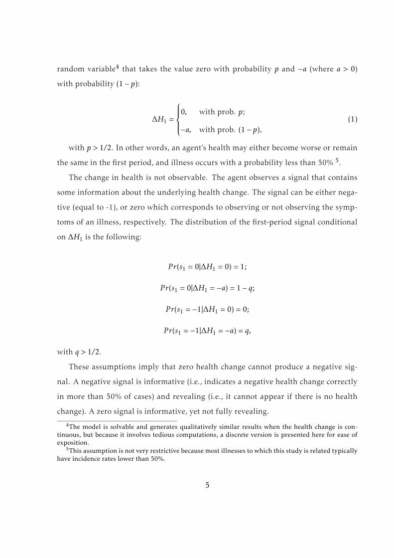
random variable4 that takes the value zero with probability p and −a (where a > 0)

with probability (1− p):

∆H1 =

0, with prob. p;

−a, with prob. (1− p),(1)

with p > 1/2. In other words, an agent’s health may either become worse or remain

the same in the first period, and illness occurs with a probability less than 50% 5.

The change in health is not observable. The agent observes a signal that contains

some information about the underlying health change. The signal can be either nega-

tive (equal to -1), or zero which corresponds to observing or not observing the symp-

toms of an illness, respectively. The distribution of the first-period signal conditional

on ∆H1 is the following:

P r(s1 = 0|∆H1 = 0) = 1;

P r(s1 = 0|∆H1 = −a) = 1− q;

P r(s1 = −1|∆H1 = 0) = 0;

P r(s1 = −1|∆H1 = −a) = q,

with q > 1/2.

These assumptions imply that zero health change cannot produce a negative sig-

nal. A negative signal is informative (i.e., indicates a negative health change correctly

in more than 50% of cases) and revealing (i.e., it cannot appear if there is no health

change). A zero signal is informative, yet not fully revealing.

4The model is solvable and generates qualitatively similar results when the health change is con-tinuous, but because it involves tedious computations, a discrete version is presented here for ease ofexposition.

5This assumption is not very restrictive because most illnesses to which this study is related typicallyhave incidence rates lower than 50%.

5

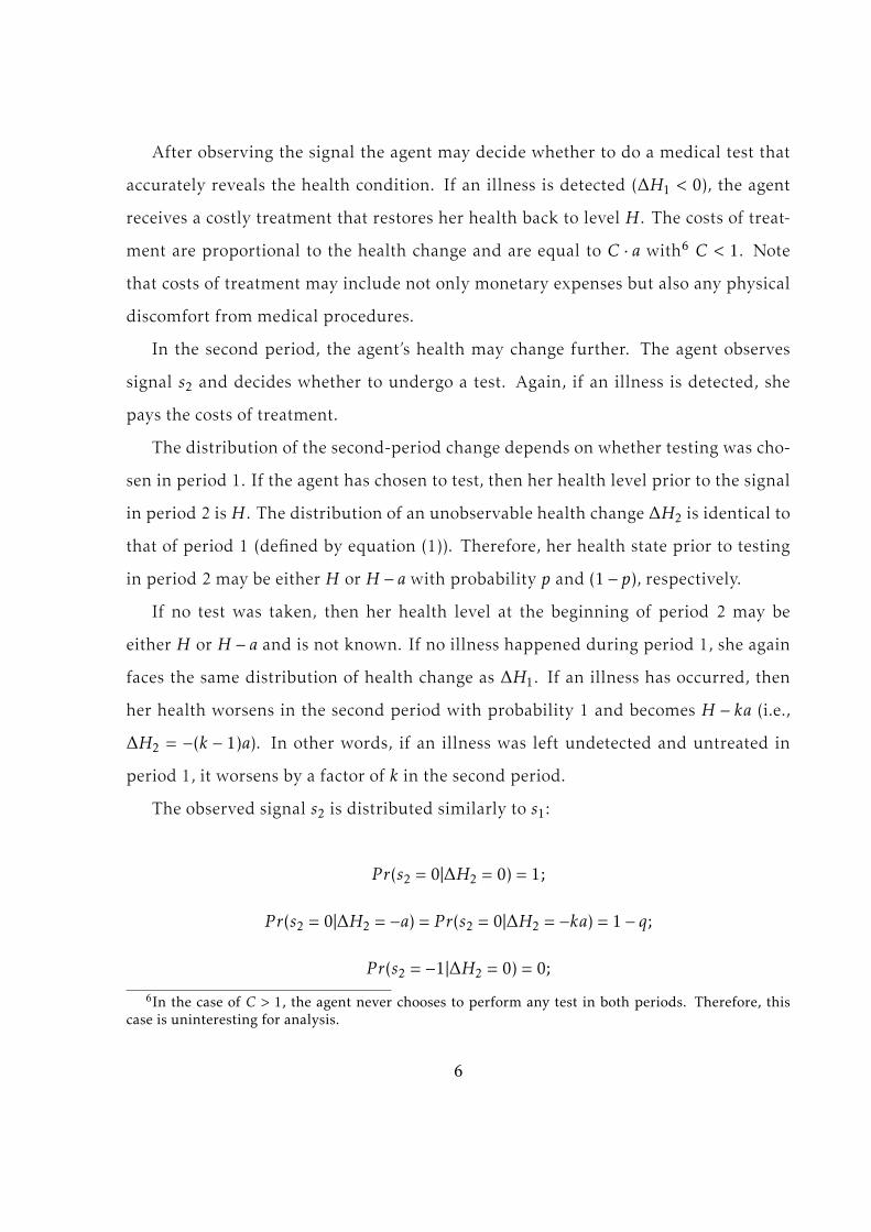
After observing the signal the agent may decide whether to do a medical test that

accurately reveals the health condition. If an illness is detected (∆H1 < 0), the agent

receives a costly treatment that restores her health back to level H . The costs of treat-

ment are proportional to the health change and are equal to C · a with6 C < 1. Note

that costs of treatment may include not only monetary expenses but also any physical

discomfort from medical procedures.

In the second period, the agent’s health may change further. The agent observes

signal s2 and decides whether to undergo a test. Again, if an illness is detected, she

pays the costs of treatment.

The distribution of the second-period change depends on whether testing was cho-

sen in period 1. If the agent has chosen to test, then her health level prior to the signal

in period 2 is H . The distribution of an unobservable health change ∆H2 is identical to

that of period 1 (defined by equation (1)). Therefore, her health state prior to testing

in period 2 may be either H or H − a with probability p and (1− p), respectively.

If no test was taken, then her health level at the beginning of period 2 may be

either H or H − a and is not known. If no illness happened during period 1, she again

faces the same distribution of health change as ∆H1. If an illness has occurred, then

her health worsens in the second period with probability 1 and becomes H − ka (i.e.,

∆H2 = −(k − 1)a). In other words, if an illness was left undetected and untreated in

period 1, it worsens by a factor of k in the second period.

The observed signal s2 is distributed similarly to s1:

P r(s2 = 0|∆H2 = 0) = 1;

P r(s2 = 0|∆H2 = −a) = P r(s2 = 0|∆H2 = −ka) = 1− q;

P r(s2 = −1|∆H2 = 0) = 0;

6In the case of C > 1, the agent never chooses to perform any test in both periods. Therefore, thiscase is uninteresting for analysis.

6

P r(s2 = −1|∆H2 = −a) = q,

with q > 1/2. The assumption that P r(s2 = 0|∆H2 = −a) = P r(s2 = 0|∆H2 = −ka) is not

crucial for the results of the model. It generates identical results if the probability of

observing a neutral signal decreases with worsening health. Note here that a negative

signal is not fully revealing (unlike in period 1). It may indicate a health change of

either −a or −ka.

The costs of treatment can be either 0, Ca or Cka depending on the detected health

change.

2.2 Utility function

Define t ∈ {1,2} to be the period index, St to be the set of signals available to the agent

in period t, and At to be the action taken in period t. Note that S1 = {s1}, S2 = {s1, s2},

and At ∈ {Vt,NVt} where Vt and NVt stand for "visit" and "no visit" to the doctor in

period t respectively.

The agent’s utility function consists of two parts - emotional, which is reference-

dependent, and physical, which corresponds to physical outcomes7. To represent the

reference-dependent part of the utility function, I use the approach developed in Kah-

neman and Tversky (1979). Namely, the emotional reaction of the agent to the news

about her health level is determined as a gain-loss utility. In this case, good news about

the agent’s health is equivalent to obtaining information that her current health state

is better than her expected health level. Analogously, the agent gets bad news when

she learns that her actual health is worse than expected. The reference point here is

defined as the agent’s expectation of health after observing the signal. The reference

point may change after new information arrives. Therefore, I define it, depending on

the period, as:

7The idea of separating physical and emotional outcomes has been employed in several previousstudies. See, for example, Kőszegi and Rabin (2006,2007,2009).

7

HR,1 =H +E(∆H1|S1)

HR,2 =H +E(∆H2|S2,A1)

In each period, the agent decides whether to undergo a health test. I first define a

one-period utility that she gets from testing. This utility has an emotional part, which

is a linear value function with a kink at reference point HR,t and a loss aversion coef-

ficient equal to λ > 1. This form of emotional utility has been proposed in Köbberling

and Wakker (2005). The physical part includes costs of treatment and utility of health

H :

Ut(Vt) =

(H +∆Ht −HR,t) +C∆Ht +H, if (H +∆Ht) > HR,t (gains).

λ(H +∆Ht −HR,t) +C∆Ht +H, if (H +∆Ht) < HR,t (losses);(2)

Note that costs of treatment may arise in both cases. If the agent’s actual health has

worsened less then she expected, this will constitute an emotional gain, but she will

have to pay costs of treatment anyway. If the agent rejects the opportunity to undergo

a test (and, hence, does not resolve the uncertainty about her health), she receives a

one-period utility from her expected health level:

Ut(NVt) =HR,t (3)

Because the agent does not live more than two periods, her choice of action in pe-

riod 2 results only from comparison of expressions (2) and (3). In period 1, the agent

makes the decision by taking into account not only the first-period utility but also the

consequences of her decision for her second-period outcomes. Therefore, her overall

utility from visiting the doctor in period 1 is defined as the sum of the first-period

8

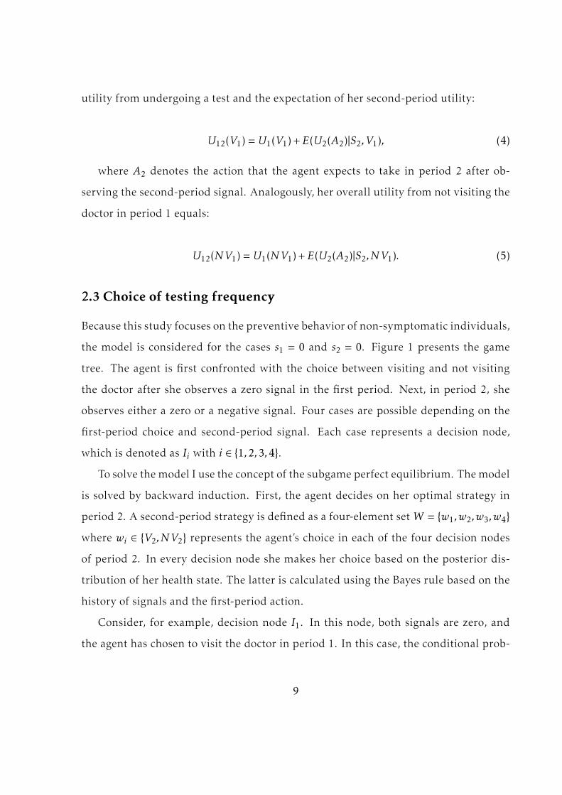
utility from undergoing a test and the expectation of her second-period utility:

U12(V1) =U1(V1) +E(U2(A2)|S2,V1), (4)

where A2 denotes the action that the agent expects to take in period 2 after ob-

serving the second-period signal. Analogously, her overall utility from not visiting the

doctor in period 1 equals:

U12(NV1) =U1(NV1) +E(U2(A2)|S2,NV1). (5)

2.3 Choice of testing frequency

Because this study focuses on the preventive behavior of non-symptomatic individuals,

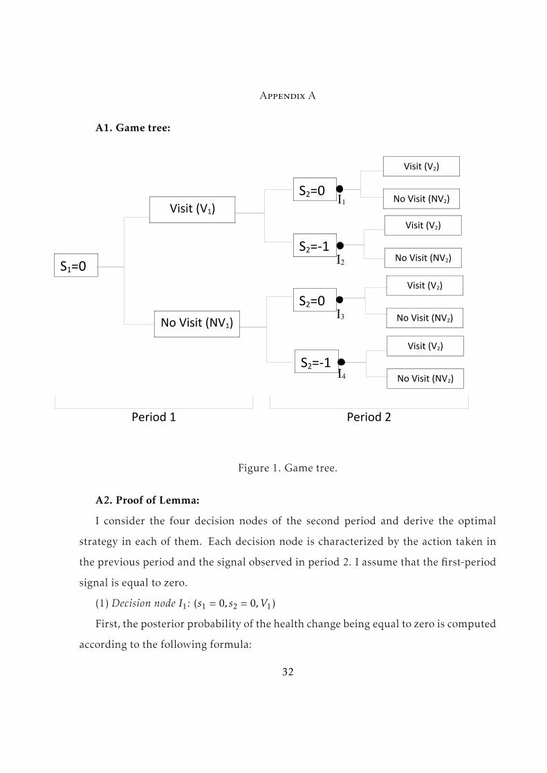
the model is considered for the cases s1 = 0 and s2 = 0. Figure 1 presents the game

tree. The agent is first confronted with the choice between visiting and not visiting

the doctor after she observes a zero signal in the first period. Next, in period 2, she

observes either a zero or a negative signal. Four cases are possible depending on the

first-period choice and second-period signal. Each case represents a decision node,

which is denoted as Ii with i ∈ {1,2,3,4}.

To solve themodel I use the concept of the subgame perfect equilibrium. Themodel

is solved by backward induction. First, the agent decides on her optimal strategy in

period 2. A second-period strategy is defined as a four-element setW = {w1,w2,w3,w4}

where wi ∈ {V2,NV2} represents the agent’s choice in each of the four decision nodes

of period 2. In every decision node she makes her choice based on the posterior dis-

tribution of her health state. The latter is calculated using the Bayes rule based on the

history of signals and the first-period action.

Consider, for example, decision node I1. In this node, both signals are zero, and

the agent has chosen to visit the doctor in period 1. In this case, the conditional prob-

9

abilities of the second health change are independent of the first-period signal. The

probability that the second-period health change is zero is recalculated in the follow-

ing way:

P r(∆H2 = 0|I1) =

=P r(s2 = 0|∆H2 = 0) · P r(∆H2 = 0)

P r(s2 = 0|∆H2 = 0) · P r(∆H2 = 0) + P r(s2 = 0|∆H2 = −a) · P r(∆H2 = −a)(6)

Therefore this probability is P r(∆H2 = 0|I1) =p

p+(1−p)(1−q) and the complementary

probability is P r(∆H2 = −a|I1) =(1−p)(1−q)

p+(1−p)(1−q) .

Next, the agent computes her reference point in node I1, which is her expected level

of health given the posterior distribution of a health change:

∆H2(I1) = −a ·(1− p)(1− q)

p+ (1− p)(1− q)(7)

Observing a negative health change after a doctor visit constitutes an emotional

loss compared to the reference point, whereas observing a zero health change consti-

tutes a gain. The agent computes her expected utility from visiting the doctor taking

into account the probabilities of a gain and a loss derived above. Note that the expec-

tation of emotional utility is always negative, independent of the probability weights

assigned to losses and gains. This utility part depends linearly on loss aversion (or

more precisely on (λ − 1)). The agent’s expected utility from visiting a doctor in this

case is8:8The details of this computation can be found in the Appendix.

10

E(U2(V2)|I1) = (8)

= −(λ− 1) · a · P r(∆H2 = −a|I1) · P r(∆H2 = −a|I1)−C · a · P r(∆H2 = −a|I1) +H

Finally, her expected utility of not visiting the doctor is calculated by the following:

E(U2(NV2)|I1) =H − a · P r(∆H2 = −a|I1) (9)

Comparing equations (8) and (9), the agent chooses whether to undergo a test. Her

choice in this case is determined by the following inequality for loss aversion (substi-

tuting for computed probabilities):

(λ− 1) <(1−C)(p+ (1− q)(1− p))

p(10)

This inequality provides a threshold for loss aversion that defines whether the agent

will undergo a test. If loss aversion is below this threshold, the agent will choose to

test, and she will choose not to test otherwise.

Similar thresholds are obtained for the choice in other decision nodes. The compu-

tations for each node can be found in the Appendix. In the node I2, a negative signal

perfectly reveals the health change. The distribution of the second-period signal after

visiting the doctor coincides with that of the first period. Observing s2 = −1, the agent

knows for sure that her health change is negative (because a negative signal can only

appear in case of a negative health change) and equals −a. In this case her health state

revealed by the doctor coincides with her reference point. As a result, her emotional

costs are equal to zero, and loss aversion does not influence her choice (she always

chooses to visit the doctor). Therefore, only the thresholds from nodes I1, I3 and I4

11

determine the agent’s choices in the second period. The corresponding thresholds are

denoted as T1, T3 and T4. These thresholds define four intervals for loss aversion. De-

pending on the considered interval the agent’s optimal behavior is characterized by

one of the four strategies described in the following lemma:

Lemma: There exist thresholds 0 < T1 < T3 < T4 such that the agent’s optimal second-period

strategy depends on loss aversion in the following way:

(1) for (λ − 1) ∈ (0,T1) the agent chooses to test in all four decision nodes (i.e. W ∗ =

{V2,V2,V2,V2});

(2) for (λ−1) ∈ (T1,T3) the agent chooses not to test in node I1 and to test in all other nodes

(i.e. W ∗ = {NV2,V2,V2,V2});

(3) for (λ−1) ∈ (T3,T4) the agent chooses not to test in node I1 and I3 and to test in all other

nodes (i.e. W ∗ = {NV2,V2,NV2,V2});

(4) for (λ−1) ∈ (T4,+∞) the agent chooses to test only in node I2 (i.e. W ∗ = {NV2,V2,NV2,NV2}).

To understand the intuition behind this lemma, consider the emotional costs of

the agent. These emotional costs depend on the reference point, which determines

the sizes of gains and losses from learning the diagnosis. The reference point in turn

depends on the second-period signal and on the previously taken action. In node I1,

the reference point is the highest among the four nodes. The agent has visited a doctor

in the first period and, hence, should not expect a large health change given the neutral

signal. In node I2, the agent receives a negative signal, which shifts her reference point

downwards. In node I3, the reference point is even lower. Although the agent observes

a neutral signal, she is in a more uncertain situation: her expected health change may

be larger because an undetected illness from period 1 may have progressed. Finally,

the lowest reference point is in node I4. Here, the negative signal definitely means

worsening of health, possibly as large as −ka.

12

As the reference point decreases from one node to another, the expected emotional

costs decrease as well. When the reference point becomes lower, the outcome above

it provides more of a gain and the outcome below it brings less of a loss (holding

loss aversion constant). The loss aversion coefficient may then be interpreted as the

sensitivity of the agent’s decision to changes in her emotional costs. When emotional

costs are large (as in node I1), a small increase in loss aversion produces a large increase

in emotional costs and, hence, leads the agent to switch from testing to not testing.

When the reference point decreases, a larger change in loss aversion is needed to make

the agent switch. Hence, the threshold defining refusal to test increases when moving

from one node to another. This is exactly what is described in the Lemma.

The agent’s problem is analogously solved in period 1 for each agent’s second-

period optimal strategy. The agent observes a zero first-period signal and computes

the overall expected utility from visiting and not visiting the doctor in period 1. As

stated in equations (4) and (5), this utility consists of two components: expected utility

of the first and second periods, respectively. The first part is defined by equation (2).

To compute the expected second-period utility, the agent first calculates the probabil-

ity of getting into every decision node of period 2 given her action and the first-period

signal. Then, she multiplies these probabilities by the utility that she expects to obtain

in every decision node given her second-period strategy. Because the agent may have

four different strategies in period 2, the solution to her problem then generates four

cases. Analogously to period 2, the agent’s first-period decision depends on loss aver-

sion. This gives four first-period thresholds that determine whether the agent chooses

to test. Combining these thresholds with those obtained in period 2, I derive the inter-

vals for loss aversion in which the agent chooses to test in both periods, in one period

or not at all. The following proposition holds9:

9See the Appendix for a detailed calculation.

13

Proposition 1: In the subgame perfect equilibrium given that s1 = 0, C < 1 and p,q > 1/2

there always exist thresholds 0 < L1 < L2 such that:

(1) for (λ− 1) ∈ (0,L1) the agent chooses testing in both periods;

(2) for (λ− 1) ∈ (L1,L2) the agent chooses testing only in period 1;

(3) for (λ− 1) ∈ (L2,+∞) the agent chooses not to test in any period.

This proposition states that the frequency of testing decreases with loss aversion.

Let us consider the intuition behind this result. The agent makes a choice in period

1, taking into account her expected utility of period 2. Her trade-off involves not

only current emotional costs and utility of treatment, but also the possibility to avoid

larger physical costs in the future. This choice is again characterized by a threshold.

If loss aversion is lower than the minimum between the first-period threshold and T1,

the agent will undergo testing in both periods. When loss aversion increases beyond

this level, the agent rejects testing in the second period. This happens because the

second period is the last one, and testing does not bring additional future benefits

(e.g., avoiding a large health loss in the future). Finally, when loss aversion is above

threshold L2, the agent’s emotional costs in the first period become so large that they

override future benefits of testing. As a result, the agent decides not to test in any

period when loss aversion is large enough.

I analyze the behavior of thresholds L1 and L2 with respect to the risk of illness as

determined by the probability (1− p). The following proposition holds10:

Proposition 2:

(1) The agent is more likely to choose testing in both periods versus testing only in one period

when the probability of being ill (1− p) increases (i.e., the threshold L1 decreases in p);

(2) There exist parameter values of k and q such that the agent is less likely to choose testing

10See Appendix for the proof.

14

in one period versus not testing at all when the probability of being ill (1− p) increases (i.e.,

there exist functions f1(q) and f2(q), monotonously decreasing and increasing in q, respec-

tively, and such that for any f1(q) < k < f2(q), the threshold L2 increases in p).

Suppose that loss aversion is below L2, and the agent has chosen to test in the first

period. The threshold L1 determines whether the agent will choose to test in period 2.

The first part of the proposition means that the frequency of testing depends positively

on the risk of illness. When the risk of illness increases, the agent becomes more likely

to test twice rather than once. An increase in the risk of illness has several effects on

the agent’s utility. First, it reduces the expected health of the second period, which

increases the expected physical benefits of treatment. The expected costs of treatment

increase as well, but because C < 1, the net benefits of treatment rise. Second, the

larger risk of illness reduces the agent’s reference point. This effect reduces the emo-

tional costs of testing by increasing gains and reducing losses relative to this reference

point. Finally, an increased risk of illness lowers the posterior probability of ∆H2 = 0

after observing a zero signal. The first two effects make testing in the second period

more attractive. The third effect works in the opposite direction. However, because, by

assumption, p,q > 1/2, the overall effect of an increase in the risk of illness is to encour-

age the agent to test more often. Because this happens for any value of loss aversion,

the threshold L1 increases with risk.

The second part of the proposition describes the choice between testing only in

period 1 and not testing at all. Here, the agent knows that her loss aversion is large

enough to make her reject testing in the second period. However, if loss aversion is

smaller than L2, she may still choose to test in the first period. An increase in the

probability of illness will diminish the emotional costs of testing due to the same ef-

fect described above. However, a higher risk of illness may have the opposite effect on

the second-period expected utility. When the agent makes a decision to test in the first

15

period, she does not know which signal she will observe in period 2. Therefore, she

has to compare the expected utility that she may obtain in period 2 after testing early

versus not testing. If she chooses not to test, she runs the risk of a large decrease in

health due to the factor k > 1 if an illness is left untreated. This, in turn, lowers the ref-

erence point in the second period. As a result, when the risk of illness rises, the agent

may prefer to delay testing until she observes symptoms in period 2. This enables her

to save emotional costs in the first period and reduce them in the second period by al-

lowing her reference point to adjust downwards. The direction in which the threshold

L2 moves in response to the increase in risk depends on which of the opposing effects

dominates. When k is not very large, the gains of delaying the test until symptoms are

observed will override the potential higher costs of treatment. Hence, L2 will depend

negatively on the risk of illness (i.e., increase in p) when k is not too large.

Propositions 1 and 2 allow us to derive the following testable predictions:

Hypothesis 1: The frequency of preventive checkups for people who do not observe any

symptoms of an illness and are not diagnosed with it depends negatively on their level of loss

aversion.

Hypothesis 2: The negative effect of loss aversion on the frequency of tests is larger for

people with higher subjective risk.

In the remainder of the paper I provide empirical support for these hypotheses.

3. Data

3.1 Data sources

The data used in this paper were collected by means of a questionnaire study specif-

ically designed for this purpose. The questionnaire study was conducted in August

2010 as a separate study within the Longitudinal Internet Studies for the Social Sci-

16

ences (LISS) panel11 of the CentERdata (Institute for Data Collection and Research at

Tilburg University, Netherlands). The data on loss aversion were obtained in a separate

wave in March 2011.

The questionnaire was administered to a representative sample of the Dutch pop-

ulation above 40 years old. It was conducted by internet. In the LISS panel the re-

spondents who do not have internet access are provided with a device allowing them

to access and complete the survey via their television set. The total number of respon-

dents who completed both questionnaires is12 3006.

The socio-economic characteristics of the respondents are available for all partic-

ipants of the LISS panel and did not require collection by means of a questionnaire.

Table 2 in Appendix B3 presents summary statistics and sample composition for those

characteristics. Since 2007, participants of the LISS panel are invited to complete an

annual core study that contains a separate health-related module. I use some of the

variables in this module (measured in 2009 (wave 3)) as additional control variables.

In this study I focus on several conditions and illnesses for which taking preventive

measures is particularly important because a long delay can significantly worsen the

long-term prognosis. These include hypertension (which increases the risk of a heart

attack and stroke), high blood sugar level (which is associated with diabetes), chronic

lung disease (such as chronic bronchitis or emphysema), and cancer.

The questionnaire began by asking whether the respondent has experienced the

symptoms of the conditions of interest. For every disease, the respondents were asked

11Further information on the structure and functioning of this panel is available at www.liss.nl12The total number of respondents who received an invitation to complete the main survey (without

the loss aversion section) was 4640. The response rate was 80.3% (3725 respondents), and a total of 3702completed questionnaires were received. The wavemeasuring loss aversion was sent to a sample of 4252people and completed by 3465 (81.5%) respondents, most of whom also participated in the first wave.The second sample does not completely match the first one. Members of the LISS panel are restrictedin the number of questionnaires they can complete during a month (they usually receive approximately4-5 questionnaires). Hence, some people from the first wave did not appear in the second wave becausethey had already completed the maximum number of questionnaires for that month. In addition, thesecond wave contains respondents who did not participate in the first wave for the same reason.

17

a Yes/No question about whether they have ever thought that they might be develop-

ing it. Next, they were presented with lists of symptoms typical for each of the four

conditions (high blood pressure/hypertension, high sugar level/diabetes, chronic lung

disease, any type of cancer) and asked to indicate whether they had ever experienced

any of those symptoms on a regular basis (i.e., Yes/No for every group of symptoms).

Table 1 presents the lists of symptoms given to the respondents. Next, they were asked

whether those symptoms were still present, whether they had ever consulted a doctor

about them and whether they had been diagnosed with a disease (and if so, when).

This information filters out the group of non-symptomatic undiagnosed respondents,

who are the primary interest in this study. The prevalence rate of the symptoms that

are mentioned in Table 1 and the diagnosis rates in the sample (both as reported by

the participants of the study) are presented in Table 2 (see Appendix B3). This table

also provides summary statistics of the background variables for the subsamples of

undiagnosed non-symptomatic individuals.

Two specific main variables that are interesting are the frequency of preventive

tests for these respondents and the individual degree of loss aversion. In addition, a

measure of subjective risk is elicited to test the second hypothesis. Below, I describe

the procedures used to obtain these variables.

3.2 Measuring frequency of preventive tests

Preventive measures correspond to the four conditions in the following way:

- high blood pressure/hypertension: blood pressure test;

- high blood sugar level/diabetes: blood test to determine the blood glucose level;

- chronic lung disease: chest X-ray;

- cancer: any non-invasive procedure for cancer screening (such as mammogram,

Pap smear test, blood test, any kind of screening, etc.).

I explore separately the frequency of cancer tests performed in a hospital and

18

the frequency of self-tests for cancer. Examples of self-tests for cancer include self-

examination of the breasts for breast cancer, detecting the presence of blood in the

stool for colon cancer, self-examination of the cervix for cervical cancer, visual inspec-

tion of the mouth for signs of oral cancer, etc.

The respondents had to indicate how often they performed tests for the 4 conditions

described above. The frequencies of blood pressure tests and sugar level tests were

measured as categorical variables, with answers falling into one of 8 categories:

(1) Never;

(2) Every few years;

(3) Once a year;

(4) 2 times a year;

(5) 3-4 times a year;

(6) Every 2 months;

(7) Once a month;

(8) Once a week or more often.

To assess the frequency of lung disease tests and cancer screening, the respondents

had to indicate how often they had undergone the relevant tests in the past 10 years.

The frequency of self-tests for cancer was measured in the same way as the frequencies

of blood pressure and sugar level tests.

3.3 Measuring loss aversion

The standard procedures for eliciting loss aversion have mostly been applied in the

monetary domain. Studies eliciting risk preferences, and particularly loss aversion in

health care, are scarce. The study by Abellan-Prepinan et al. (2009) exploring risk

preferences in health outcomes adopts the estimates of the loss aversion coefficient

obtained for the monetary domain in Tversky and Kahneman (1992). In Stalmeier and

Bezembinder (1999), the loss aversion coefficient is estimated for the choice between

19

some impaired health state as a status quo and a gamble with possible improvement

or worsening of health. Bleichrodt and Pinto (2002) estimates the significance of the

loss aversion phenomenon in the domain of health using riskless choice questions.

One important problem that arises in eliciting loss aversion is separating the risk

preferences stemming from the utility curvature (risk aversion) from those evoked by

the disproportional weight put on losses compared to gains (loss aversion).13.

Several studies have filtered out different components of risk preferences. These

techniques usually imply stating indifference in a series of choices comparing two lot-

teries with changing outcomes or probabilities (Booij and van de Kuilen(2009), Wakker

and Deneffe (1996)). These procedures often result in a high non-response rates in

general population studies because the task becomes too complicated for many peo-

ple. Stating indifference in lotteries presented in terms of health outcomes may be

even less accessible for the respondents than when the lotteries are presented in terms

of money. On the other hand, employing a less complicated elicitation procedure may

not deliver enough information to derive a good measure of loss aversion.

In this study, I aim to balance these conflicting issues. To preserve the representa-

tiveness of the sample and yet obtain a reasonable proxy for loss aversion in a series

of acceptance/rejection questions, I elicit indifference between the lotteries in life ex-

pectancy and a fixed reference outcome. The reference outcome is fixed at the respon-

dent’s perceived life expectancy. The respondent is presented with a series of binary

choice questions (accepting or rejecting a lottery). Each lottery is a 50-50 probability

lottery with a positive outcome being an increase in life expectancy by 10 years. The

negative outcome is varied from the loss of 0 years of the current life expectancy up to

10 years14. The value of loss aversion is recorded from the midpoint between the last

13According to prospect theory, probability weighting may also influence risk preferences: people aregenerally found to overstate large and understate small probabilities. In this study, respondents face 50-50 lotteries. Empirical evidence suggests that probability distortions are minimized around the middleof the probability scale (Gonzalez and Wu(1999), Wu and Gonzalez(1996)).

14The examples of the questions for this procedure can be found in Appendix B2.

20

accepted lottery and the rejected lottery. Loss aversion is computed according to the

following formula: LA = 10/(n−3/2), where n is an index of the rejected lottery. For ex-

ample, if the respondent rejects the lottery offering (+10, -4) but accepts all preceding

lotteries, his/her loss aversion coefficient is recorded as 2.86 (because this is the fifth

lottery in the sequence). People who answer "Yes" to all 11 lotteries are assigned loss

aversion equal to 1. Respondents who rejected the very first, "harmless", lottery with

the negative outcome being zero are assigned loss aversion of15 58.

Although this procedure does not allow me to perfectly separate loss aversion (in

the sense of relatively heavier losses versus gains) from the utility curvature, I argue

that the choice in this task is to a large extent driven by loss aversion. First, the re-

spondents face lotteries with a clearly stated reference point. Positive and negative

outcomes here are unambiguously coded with respect to a given point of comparison,

which is the perceived life expectancy. Previous studies have shown that loss aversion

is typically more pronounced in choices with a clearly stated reference point. For ex-

ample, Hjorth and Fosgerau (2011) find more evident loss aversion in cases when the

reference point is more firmly established. In Ritov and Baron (1993), manipulating

the salience of the reference point leads to changes in the subjects’ behavior in risky

choices: when the status quo is more salient fewer subjects demonstrate indifference

in choices between risky options. Koop and Johnson (2010) argues that salience may

be an important condition for an outcome to become a reference point.

Second, many studies find that the status quo, the respondent’s expectation of the

outcome, or the respondent’s aspiration level of the outcome usually serve as points of

comparison evoking loss aversion. Several studies support the status quo bias in the

domains of goods and money (Knetsch (1989), Schweitzer (1994)). Koszegi and Rabin

15Formally, it is impossible to derive loss aversion for this group of respondents because there is nomidpoint. In other words, their loss aversion can be infinitely large. However, it is desirable to assigna certain value for them, and this value should be on the same "scale" as all other values. To do this, Ibuild a curve that connects all 11 points representing the loss aversion values. I then approximate itwith a polynomial of degree 6 (which appears to be an optimum) and find that the value predicted bythis polynomial is approximately 58.

21

(2006) argue that the status quo may also be interpreted in terms of expectation if a

person does not expect her status quo to change. Van Osch et al. (2006) finds that

a sure outcome presented in the lottery choices involving life expectancy serves as a

reference point for the majority of subjects. Harinck et al. (2007) lists several studies

confirming that loss aversion is more relevant for anticipated rather than experienced

outcomes. Neuman and Neuman (2008) uses a discrete-choice experiment to confirm

that loss aversion arises with respect to the status-quo scenario given to the subjects.

It is easy to see that perceived life expectancy used as a point of comparison in the

present study satisfies all mentioned definitions of a reference point. Life expectancy

by definition is an individual’s expected length of life. It may indicate an aspiration

of life duration. At the same time, it is also presented as a status-quo scenario as the

respondents do not have any better estimate of their life duration than their perceived

life expectancy. All of this makes perceived life expectancy a likely candidate for the

reference point in this study.

Finally, to derive a proxy for loss aversion, I use mixed gambles, i.e., gambles in-

volving both gains and losses. This makes the concept of loss aversion particularly

relevant. If the lotteries offered to the respondents were framed solely in terms of

gains or losses, then loss aversion would not be able to explain observed lottery choices

(Wakker (2010)). Brooks and Zank (2004) find that once a loss outcome is introduced

to a pure gain lottery, most subjects shift in the direction of loss aversion.

Several points should be made regarding the use of this proxy for loss aversion in

regressions.

First, loss aversion is normalized to the interval from 0 to 1, with the first-lottery re-

jecters receiving the value 3. Table 3 (in Appendix B4) presents the list of loss aversion

values with their corresponding frequencies in the sample. Normalized loss aversion

gives an objectively better fit of the data compared to the logarithm of non-normalized

loss aversion: in the regressions with identical numbers of observations and sets of ex-

22

planatory variables, it produces a higher pseudo R-squared and higher likelihood ratio

and higher significance of loss aversion itself.

Second, as a robustness check, I present regression results excluding respondents

who have rejected the "harmless" lottery (with zero loss in health). People may be

rejecting this lottery for various reasons not directly related to loss aversion. For ex-

ample, they may have an aversion to any kind of medical procedure or may not be able

to imagine a treatment with no side effects. Such beliefs may decrease the frequency

of testing without relation to loss aversion.

Finally, the group of respondents who answered "Yes" to all loss aversion questions

is not included in the sample. Although this group constitutes only 2-3% of the sample

in regressions (depending on the illness), it has a disproportional influence on the esti-

mated effect of loss aversion and on its statistical significance. For example, inclusion

of these observations in the regression for sugar level tests (only 2.5% of the sample)

increases the p-value for loss aversion almost threefold. In the empirical analysis liter-

ature, such observations are typically called "fringeliers", i.e., observations that do not

greatly stand out in the sample (usually approximately 3 standard deviations from the

mean) and yet "occur more often than seldom" (Wainer (1976)). It has been found that

inclusion of the fringeliers may significantly increase the error variance and reduce the

power of statistical tests (Osborne and Overbay (2004)). Deleting these observations

is recommended as one potential way of dealing with them (Hancock (2010), p.62). I

follow this practice when presenting the main results of the study, but the results of

regressions, including the fringeliers, are also presented in the Appendix as a robust-

ness check16.

16Note that the respondents may be assigned to this group just by answering "Yes" to every loss aver-sion question without careful consideration. A suggestive fact is that the average time spent per ques-tion by the respondents in this group is 14 seconds, which is much lower than the average of 63 secondsfor the rest of the sample. Another reason for such responses may be the acquiescence bias (so-called"yeah-saying"; Fischhoff and Manski (2000)).

23

3.4 Measuring subjective risk

To measure subjective risk of illness, respondents were asked to indicate how likely

they believe it is that they will develop an illness in their lifetime. They were asked

to state this likelihood using a number between 0 and 100. However, this measure

does not give any information on whether a respondent views this risk as high, low or

average. In addition, as previous general population studies have shown, the stated

probability of being ill may be far from its epidemiological estimates (see Carman

and Kooreman (2011)). To address this problem, I ask the respondents to indicate the

number of people out of 100 from the same socio-economic group who they estimate

will develop an illness in their lifetime. The ratio of these two measures allows me to

classify respondents into three groups. If this ratio is larger than 1, a person belongs

to the above-average risk group; if it is smaller than 1, to the below-average risk group;

and if it is exactly 1, to the average-risk group. For example, if an individual estimates

her own risk to be 10% but states that only 5 people out of 100 will develop an illness,

then she is classified as a subjectively high-risk person.

4. Empirical Results

For every particular illness, I focus on people who report that they have never had

any of the mentioned symptoms on a regular basis and have never been diagnosed

with it. The analysis of the stated frequencies of preventive testing reveals that many

people choose not to undergo any tests at all. Tables 4-8 present the distributions of

stated testing frequencies for each disease. The first two columns show the number

of respondents and their fraction in the whole sample, and columns 3 and 4 show the

same information in the subsample of non-symptomatic undiagnosed respondents.

For cancer screening, the breakdown of answers for men and women is combined.

We observe that from 25 to 75% of the population report a zero frequency of tests

depending on the illness. For cancer screening, this number goes up to 85% for men

24

and 65% for women17. Therefore, I separately study the factors that influence the

decision to participate in preventive testing and those that determine the frequency of

testing among participants. For this purpose, I employ a two-part model (Leung and

Yu (1996)). For each disease, I first run a probit regression with a binary dependent

variable equal to zero if a person does not undergo a relevant test and 1 if he/she

chooses any positive frequency of testing. Next, I run either an ordinary logit or an

OLS regression (depending on the way frequency is measured) with the dependent

variable being the frequency of tests. These regressions are restricted to the sample

of those who reported a non-zero frequency18. For each regression, I present both the

long and the short versions (i.e., excluding nonsignificant regressors).

First, consider blood pressure and sugar level tests (Tables 9 and 10). The first and

second columns of these tables present the estimation results for the probit model.

The estimation results show that loss aversion is a statistically significant factor that

discourages people from preventive testing. The decision to participate in testing is

positively influenced by such factors as age, body mass index (BMI), having a family

history of a disease, visiting a family physician more often and worrying about a dis-

ease19. Increased smoking and alcohol consumption are associated with a lower prob-

ability of preventive testing (although not significantly for alcohol). Variables showing

how many cigarettes a person smokes and how much alcohol she consumes may be

indicative of a more general attitude towards health. People in whom these levels are

high may be less likely to care about their own health and, therefore, less inclined to

adopt preventive measures.

17This difference is likely due to the existence in the Netherlands of publicly funded programs forbreast cancer and cervical cancer screening for women, but no cancer screening program for men.

18An alternative way to perform this analysis would be by means of the Heckman selection model.However, a commonly indicated distinction between the two is that the Heckman model is more appro-priate when one needs to predict values of the outcome as if there was no selection. The two-part modelis more suitable for the situation when one needs to analyze the actual outcome (see, for example, Leungand Yu (1996) for a discussion). The latter is closer to the present case.

19Table 28 contains a detailed description of all control variables.

25

Columns 3 and 4 of the same tables contain estimation results for the frequency of

preventive check-ups among those respondents who have decided to undergo a test.

Regressions are ordered logit because the dependent variable (frequency of tests) is

categorical. The set of regressors does not change because the same factors may influ-

ence testing frequency. Loss aversion is not significant. Other factors contributing to

more frequent testing are older age, visiting a family physician and worrying about a

disease more often.

Table 11 shows similar results for lung disease testing. Regressions for lung dis-

ease do not contain variables from the LISS core study of 2009 because the period for

which the frequency of lung disease tests is measured extends to 10 years. Hence, the

variables from 2009 are irrelevant for earlier decisions to test. However, I add other

variables that may influence this decision. These are the number of times a person

has had the flu, the number of times she received a flu shot and a binary variable in-

dicating whether the respondent gets colds easily. All of these factors may increase

adherence to preventive testing. I expect the effect of flu shots to be positive because a

person who receives flu shots frequently may either be more conscious about his/her

health or have some underlying condition that makes him/her susceptible to both flu

and lung disease.

The results for lung disease are similar to those for blood pressure and sugar level

testing. Loss aversion is found to be a significant and negative factor in the decision to

undergo a test for lung disease. However, it is not significant for the choice of testing

frequency above zero.

The effect of loss aversion on cancer screening is explored in two different dimen-

sions: cancer screenings in hospitals and self-tests for cancer. In the Netherlands,

screening programs for female-specific types of cancer are publicly funded for women

in certain age groups: the government provides breast cancer screening every 2 years

for women between 50 and 75 years old, and cervical cancer screening is funded ev-

26

ery five years for women between 30 and 60 years old. There is no cancer screening

program for men. Therefore, one might expect that the decision to participate in pre-

ventive screening and the effect of loss aversion on this decision would differ between

men and women. To account for this possibility, loss aversion is multiplied by the

dummy variables for gender. In addition to the standard control variables, I include

the average number of screening programs for which a person was eligible during the

past ten years20. I find that the discouraging effect of loss aversion on the participation

decision is not significant for either gender (Table 12). Worrying about cancer, having

a family history and eligibility to enter a screening program are the most important

factors in this decision. The influence of loss aversion on the frequency of medical

tests is not statistically significant, but the size of the effect is larger for men than for

women.

Table 13 shows that loss aversion is marginally significant in the decision to partic-

ipate in testing and significant at the 10% level for the frequency of testing for women.

However, no significant effect is observed for men. The set of control variables is the

same as for medical cancer tests. Although self-tests by definition do not require a visit

to the hospital, the average number of accessible screening programs is still included

for the simple reason that a woman undergoing a medical test for cancer also has more

access to information on self-testing. As Table 13 shows, the number of available pro-

grams is indeed a significant positive factor.

For the regressions where loss aversion is significant, I perform two robustness

checks (Tables 14-17). First, I examine how the results change when the respondents

with the highest loss aversion are excluded (group 1). Second, I present the estima-

tion results when the group of loss-neutral individuals (group 12) is included in the

regressions. We observe that exclusion of people with the highest loss aversion does

20For men, this variable is always zero. For women, this variable can be 0, 1 or 2. I compute a weightedaverage, taking into account the number of years out of the past ten that a woman has been eligible foreach of these screenings. An example of this computation can be found in Table 20.

27

not change the sign of the loss aversion effect for blood pressure, blood sugar and lung

disease testing. For blood pressure and lung disease testing, the effect is also most

stable in terms of statistical significance. Loss aversion is a significant and positive

predictor of cancer self-test frequency among men. However, only 125 men remained

in this subsample, which may not be enough to obtain a correct estimate of the effect.

For women, the effect on self-test frequency seems to be driven by the excluded indi-

viduals. This situation may reflect the fact that women who have a greater aversion to

medical procedures also reject the harmless lottery more often. Finally, as mentioned

earlier, the inclusion of loss-neutral individuals greatly reduces the significance and

size of the loss aversion estimates, although this group constitutes only 2 to 3% of the

sample. This result is consistent with the view of these observations as "fringeliers".

Tables 18-22 present the estimates of the marginal effects in the main regressions.

For brevity, I consider only regressions without nonsignificant parameters. I present

marginal effects for a unitary and a one-standard-deviation change in each regres-

sor, keeping other variables at their mean levels. From marginal effects for the probit

model, I find that an increase of the loss aversion logarithm by one increases the proba-

bility of non-participation in testing by 1.4-1.8 percentage points. For blood pressure,

blood sugar and lung disease, the size of the loss aversion effect is similar to or larger

than the effect of obtaining one additional level of education21. The effect for self-

testing for cancer for women is in a similar range. As explained earlier, loss aversion is

not significant in the probit regression for medical cancer tests, but it produces a large

effect on testing frequency among both men and women who have decided to undergo

testing.

Because the logarithm of loss aversion may be not very intuitive for interpretation,

I also consider the predicted probability of participation in testing given different lot-

21Note, however, that the influence of education on the decision to test may be positive or negative.On the one hand, education may increase awareness of the benefits of testing, exerting a negative effecton the probability of non-testing. On the other hand, more educated people are less likely to engage inhealth-worsening activities, which may increase the probability of non-testing (Chen and Lange (2008)).

28

tery rejection choices (which correspond to different loss aversion values) and mean

values of other variables. Table 23 presents the results. The difference in the predicted

probability of testing between a person rejecting the first lottery (and therefore having

the highest possible loss aversion) and a person accepting all lotteries except the last

one can be as large as 10 to 13 percentage points. In other words, being willing to sacri-

fice one additional year of life expectancy with a 50 percent chance of winning 10 additional

years of life expectancy is associated with an increase of roughly 1.1-1.3 percentage points

in the probability of testing.

Finally, I analyze whether the effect of loss aversion differs in various risk groups.

Tables 24-27 present the results. In these regressions, the low-risk group is taken as a

benchmark. The first row shows the effect of loss aversion in this benchmark group,

and the other two estimates indicate how much the effect differs from this benchmark.

We observe that, for the blood pressure, blood sugar and lung disease tests, the ab-

solute loss aversion effect is consistently larger in the high-risk group. People who

consider themselves to be at higher-than-average risk are more influenced by loss aver-

sion in their decision to test for these illnesses. The same pattern is observed for the

frequency of self-tests for cancer among women22. The difference between the groups

is not statistically significant, possibly because both loss aversion and the risk ratio

appear to be very noisy measures.

5. Conclusions

The theoretical and empirical analysis in this paper helps to establish a link between

two important phenomena: loss aversion and information aversion in the context of

health care decision making. It is shown that loss aversion is a significant contribu-

tor to infrequent preventive testing among non-symptomatic people. A person has to

22In the case of cancer testing, the average- and high-risk groups have been merged together becausethe average-risk group becomes too small.

29

make a choice about his/her frequency of preventive check-ups, which constitutes a

trade-off. On the one hand, learning health information more frequently allows a per-

son to detect an illness earlier and, hence, to receive a less costly treatment. On the

other hand, learning a bad diagnosis is emotionally distressing, and a person may pre-

fer to avoid it. The model shows that the frequency of testing depends negatively on

loss aversion, which is the main driving force behind health anxiety. Empirical analysis

supports this theoretical prediction. I construct an individual proxy for loss aversion,

measured by the lottery choice questions with respect to life expectancy, and relate it

to the frequency of tests for four illnesses: hypertension, diabetes, chronic lung disease

and cancer. Although these conditions differ in their controllability and consequences

for life duration, the loss aversion effect is quite stable across all of them. The size

of the effect is statistically and economically significant. Moreover, the negative effect

of loss aversion is higher in magnitude for people who consider themselves to be at

above-average risk of illness.

The policy implications that can be derived from this analysis relate to the meth-

ods of encouraging people to use preventive testing. One of these methods involves

distributing messages and informational booklets about the importance of preventive

testing. It has been found that framing of those messages in terms of either gains or

losses may influence their efficiency. For example, it is often argued that loss-framed

messages may induce an instinct to avoid losses, leading to a higher uptake of preven-

tion (Rothman et al. (2006)). The results of the present study, however, suggest that

this strategy may give rise to the ostrich effect, thus generating the opposite behavior,

especially in a high-risk population. A more efficient measure in this case would be to

increase the perceived effectiveness of treatment. In the present model, it is assumed

that treatment allows the individual to restore his/her health to its initial level. In real-

ity, this may not be the case. If a person thinks that her health may only be restored to

some low level, then her likelihood of testing will be decreased. Therefore, informing

30

the population about cases of successful treatment or high disease controllability may

outweigh the ostrich effect, at least for some people.

31

Appendix A

A1. Game tree:

S1=0

Visit (V1)

No Visit (NV1)

S2=0

S2=-1

S2=0

S2=-1

Visit (V2)

No Visit (NV2)

Visit (V2)

No Visit (NV2)

Visit (V2)

No Visit (NV2)

Visit (V2)

No Visit (NV2)

I1

I2

I3

I4

Period 1 Period 2

Figure 1. Game tree.

A2. Proof of Lemma:

I consider the four decision nodes of the second period and derive the optimal

strategy in each of them. Each decision node is characterized by the action taken in

the previous period and the signal observed in period 2. I assume that the first-period

signal is equal to zero.

(1) Decision node I1: (s1 = 0, s2 = 0,V1)

First, the posterior probability of the health change being equal to zero is computed

according to the following formula:

32

P r(∆H2 = 0|I1) =P r(s2=0|∆H2=0)·P r(∆H2=0)

P r(s2=0|∆H2=0)·P r(∆H2=0)+P r(s2=0|∆H2=−a)·P r(∆H2=−a)

Therefore, the posterior probabilities of the possible health changes in this node are

the following:

P r(∆H2 = 0|I1) =p

p+ (1− p)(1− q)(11)

P r(∆H2 = −a|I1) =(1− q)(1− p)

p+ (1− p)(1− q)(12)

(13)

Next, the expected health level in node I1 is:

∆H2(I1) = −a ·(1− p)(1− q)

p+ (1− p)(1− q)(14)

Because, in this decision node, only two health changes are possible, the larger of

them brings a gain and the smaller brings a loss with respect to the reference point.

This allows me to compute the agent’s emotional utility Em2 in case she decides to

undergo a test:

E(Em2|I1) = (0−∆H2(I1))p

p+ (1− p)(1− q)+λ

(−a−∆H2(I1)

) (1− q)(1− p)p+ (1− p)(1− q)

=

= −(λ− 1)ap(1− q)(1− p)

(p+ (1− p)(1− q))2(15)

The total utility of visiting the doctor in node I1 according to equation (8) is:

EU (V2|I1) = −(λ− 1)ap(1− q)(1− p)

(p+ (1− p)(1− q))2−Ca

(1− q)(1− p)p+ (1− p)(1− q)

+H (16)

The utility of not visiting the doctor in this node is:

33

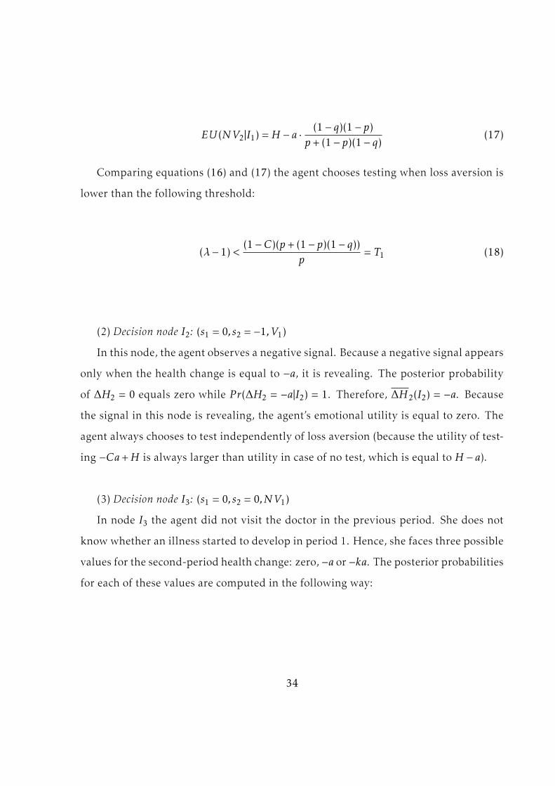
EU (NV2|I1) =H − a ·(1− q)(1− p)

p+ (1− p)(1− q)(17)

Comparing equations (16) and (17) the agent chooses testing when loss aversion is

lower than the following threshold:

(λ− 1) <(1−C)(p+ (1− p)(1− q))

p= T1 (18)

(2) Decision node I2: (s1 = 0, s2 = −1,V1)

In this node, the agent observes a negative signal. Because a negative signal appears

only when the health change is equal to −a, it is revealing. The posterior probability

of ∆H2 = 0 equals zero while P r(∆H2 = −a|I2) = 1. Therefore, ∆H2(I2) = −a. Because

the signal in this node is revealing, the agent’s emotional utility is equal to zero. The

agent always chooses to test independently of loss aversion (because the utility of test-

ing −Ca+H is always larger than utility in case of no test, which is equal to H − a).

(3) Decision node I3: (s1 = 0, s2 = 0,NV1)

In node I3 the agent did not visit the doctor in the previous period. She does not

know whether an illness started to develop in period 1. Hence, she faces three possible

values for the second-period health change: zero, −a or −ka. The posterior probabilities

for each of these values are computed in the following way:

34

P r(∆H2 = 0|I3) = P r(∆H2 = 0|I3,∆H1 = 0)P r(∆H1 = 0|I3)+

+P r(∆H2 = 0|I3,∆H1 = −a)P r(∆H1 = −a|I3) =p2

P r(s1 = 0, s2 = 0,NV1)(19)

P r(∆H2 = −a|I3) = P r(∆H2 = −a|I3,∆H1 = 0)P r(∆H1 = 0|I3)+

+P r(∆H2 = −a|I3,∆H1 = −a)P r(∆H1 = −a|I3) =p(1− q)(1− p)

P r(s1 = 0, s2 = 0,NV1)(20)

P r(∆H2 = −ka|I3) = P r(∆H2 = −ka|I3,∆H1 = 0)P r(∆H1 = 0|I3)+

+P r(∆H2 = −ka|I3,∆H1 = −a)P r(∆H1 = −a|I3) =(1− q)2(1− p)

P r(s1 = 0, s2 = 0,NV1)(21)

Finally, P r(s1 = 0, s2 = 0,NV1) = p2 + p(1− q)(1− p) + (1− q)2(1− p).

The expected health level in node I3 is:

∆H2(I3) =−ap(1− q)(1− p)− ka(1− q)2(1− p)p2 + p(1− q)(1− p) + (1− q)2(1− p)

(22)

Themaximum (∆H2 = 0) andminimum (∆H2 = −ka) outcomes of the second-period

health change constitute a gain and a loss, respectively, relative to the reference point.

The outcome ∆H2 = −a may be a gain or a loss depending on the parameter values.

For brevity, I consider the case of k < p2

(1−q)2(1−p) + 1 when ∆H2 = −a constitutes a loss.

Therefore, the expected emotional utility in node I3 is:

35

E(Em2|I3) =ap(1− q)(1− p) + ka(1− q)2(1− p)p2 + p(1− q)(1− p) + (1− q)2(1− p)

×p2

P r(s1 = 0, s2 = 0,NV1)+

+λ(−a+

ap(1− q)(1− p) + ka(1− q)2(1− p)p2 + p(1− q)(1− p) + (1− q)2(1− p)

)×

p(1− q)(1− p)P r(s1 = 0, s2 = 0,NV1)

+

+λ(−ka+

ap(1− q)(1− p) + ka(1− q)2(1− p)p2 + p(1− q)(1− p) + (1− q)2(1− p)

)×

(1− q)2(1− p)P r(s1 = 0, s2 = 0,NV1)

, (23)

where P r(s1 = 0, s2 = 0,NV1) is defined above.

The agent’s expected utility of visiting the doctor is:

EU (V2|I3) = E(Em2|I3)−C∆H2(I3) +H (24)

The expected utility of not visiting the doctor in this node is:

EU (NV2|I3) =H −∆H2(I3) (25)

Comparing these two expected utilities, the agent chooses to undergo a test when

her loss aversion satisfies the following inequality:

(λ− 1) <(1−C)(p2 + p(1− q)(1− p) + (1− q)2(1− p))

p2= T3 (26)

(4) Decision node I4: (s1 = 0, s2 = −1,NV1)

In node I4 the agent may experience two values of the second-period health change:

∆H2 = −a and ∆H2 = −ka. Since the agent observes a negative signal she knows that

36

her health change has reduced. However, the agent does not know exactly the size of

this reduction. The posterior probabilities of these values are:

P r(∆H2 = −a|I4) = P r(∆H2 = −a|I4,∆H1 = 0)P r(∆H1 = 0|I4)+

+P r(∆H2 = −a|I4,∆H1 = −a)P r(∆H1 = −a|I4) =q(1− p)p

P r(s1 = 0, s2 = −1,NV1)(27)

P r(∆H2 = −ka|I4) = P r(∆H2 = −ka|I4,∆H1 = 0)P r(∆H1 = 0|I4)+

+P r(∆H2 = −ka|I4,∆H1 = −a)P r(∆H1 = −a|I4) =(1− q)q(1− p)

P r(s1 = 0, s2 = −1,NV1)(28)

Finally, P r(s1 = 0, s2 = −1,NV1) = q(1− p)p+ q(1− q)(1− p).

The expected health change is then:

∆H2(I4) =−aq(1− p)p − ka(1− q)q(1− p)

q(1− p)p+ q(1− q)(1− p)(29)

The expected emotional utility in this node is:

E(Em2|I3) =(−a+

aq(1− p)p+ ka(1− q)q(1− p)q(1− p)p+ q(1− q)(1− p)

)×

q(1− p)pP r(s1 = 0, s2 = −1,NV1)

+

+λ(−ka+

−aq(1− p)p − ka(1− q)q(1− p)q(1− p)p+ q(1− q)(1− p)

)×

(1− q)q(1− p)P r(s1 = 0, s2 = −1,NV1)

=

= (λ− 1)(−ka+

−aq(1− p)p − ka(1− q)q(1− p)q(1− p)p+ q(1− q)(1− p)

)×

(1− q)q(1− p)P r(s1 = 0, s2 = −1,NV1)

, (30)

where P r(s1 = 0, s2 = −1,NV1) is defined above.

The utilities of visiting and not visiting the doctor are derived similarly to cases

already considered. The agent chooses to perform a test in node I4 when the following

37

inequality holds:

(λ− 1) <(1−C)(p+ k(1− q))(p+ (1− q))

(k − 1)p(1− q)= T4 (31)

I now compare the thresholds T1, T3 and T4. First, it is easy to see that threshold T1

is lower than T4. After some simplification of the inequality, we obtain:(1−C)(p+(1−q)(1−p))

p < (1−C)(p+k(1−q))(p+(1−q))(k−1)p(1−q) ;

⇒−p(1− q)− kp(1− q)2 − (1− q)2(1− p) < p2 + p(1− q)

The latter is true since the left-hand side is always negative, whereas the right-hand

side is positive. A similar procedure yields the following comparison for thresholds T1

and T3:(1−C)(p+(1−q)(1−p))

p < (1−C)(p2+(1−q)(1−p)p+(1−q)2(1−p))p2

;

⇒ p2 + p(1− q)(1− p) < p2 + (1− q)(1− p)p+ (1− q)2(1− p)

The latter holds since 0 < (1− q)2(1− p). Finally, I compare T3 and T4:(1−C)(p2+(1−q)(1−p)p+(1−q)2(1−p))

p2< (1−C)(p+k(1−q))(p+(1−q))

(k−1)p(1−q) ;

⇒ k(p2(1−q)+ (1−q)2(1−p)(p+(1−q))−p(1−q)(p+(1−q))) < p2(1−q)+ (1−q)2(1−

p)(p+ (1− q)) + p2(p+ (1− q)).

The right-hand side of this inequality is positive. Compare the left-hand side to

zero:

p2(1− q) + (1− q)2(1− p)(p+ (1− q))− p(1− q)(p+ (1− q)) < 0;

⇒ (1− q)(1− p) < p2;

The latter holds since given that p,q > 1/2, (1− q)(1− p) < 1/4 and p2 > 1/4. There-

fore, the threshold T3 is always smaller than T4. Hence, we obtain that 0 < T1 < T3 < T4.

These thresholds allow us to define the optimal strategy of the agent in period 2 for

any loss aversion interval as stated in the Lemma. Q.E.D.

38

A3. Proof of Proposition 1:

To prove Proposition 1, I consider each of the four intervals for loss aversion ob-

tained in the Lemma. In each interval, the agent’s first-period problem is solved. Com-

bining this solution with the optimal second-period strategy, I obtain the equilibrium

for each loss aversion value. In the first period, the agent compares the overall utility

of visiting the doctor and the overall utility of not visiting the doctor. The overall util-

ity takes into account not only the first-period utility, but also the expectation of the

second-period utility given the action taken in the first period. In period 1, the agent

does not know which signal she will observe in period 2. She computes the probability

of observing a zero or negative signal, given that she will visit the doctor in period 1,

in the following way:

P r(s2 = 0|s1 = 0,V1) = P r(s2 = 0|V1) = P r(s2 = 0|∆H2 = 0,V1)P r(∆H2 = 0|V1)+

+P r(s2 = 0|∆H2 = −a,V1)P r(∆H2 = −a|V1) = p+ (1− q)(1− p) (32)

P r(s2 = −1|s1 = 0,V1) = P r(s2 = −1|V1) = P r(s2 = −1|∆H2 = 0,V1)P r(∆H2 = 0|V1)+

+P r(s2 = −1|∆H2 = −a,V1)P r(∆H2 = −a|V1) = 0+ q(1− p)

Analogously, the probabilities of signals after not visiting in period 1 equal:

P r(s2 = 0|s1 = 0,NV1) = p+(1− q)2(1− p)

p+ (1− q)(1− p)

P r(s2 = −1|s1 = 0,NV1) =q(1− p)(p+ (1− q))p+ (1− q)(1− p)

(33)

(1) Consider first the interval (λ− 1) ∈ (0,T1):

39

In this interval, the optimal strategy in period 2 is to visit the doctor in every deci-

sion node. The utilities of visiting the doctor in every node are defined in the proof of

the Lemma above. By weighting themwith the probabilities (32) and (33) and combin-

ing them with the first-period utilities of visiting and not visiting the doctor, respec-

tively, I obtain the overall utilities of visiting and not visiting the doctor. Note that the

first-period utility given s1 = 0 always coincides with that of the second period in node

I1 defined in the Lemma. The overall expected utility of visiting the doctor in period

1 is:

EU12(V1) =(H −Ca

(1− q)(1− p)p+ (1− q)(1− p)

− (λ− 1)ap(1− q)(1− p)

(p+ (1− q)(1− p))2

)+ (p+ (1− q)(1− p))×

×(H −Ca

(1− q)(1− p)p+ (1− q)(1− p)

− (λ− 1)ap(1− q)(1− p)

(p+ (1− q)(1− p))2

)+ q(1− p)(H −Ca) (34)

Analogously, the overall expected utility of not visiting equals:

EU12(NV1) =(H − a

(1− q)(1− p)p+ (1− q)(1− p)

)+p2 + (1− q)(1− p)p+ (1− q)2(1− p)

p+ (1− q)(1− p)·

·(H −C

ap(1− q)(1− p) + ka(1− q)2(1− p)p2 + (1− q)(1− p)p+ (1− q)2(1− p)

−(λ− 1)p2(ap(1− q)(1− p) + ka(1− q)2(1− p))

(p2 + (1− q)(1− p)p+ (1− q)2(1− p))2

)+q(1− p)(p+ (1− q))p+ (1− q)(1− p)

(H −C

aq(1− p)p+ kaq(1− q)(1− p)q(1− p)p+ q(1− p)(1− q)

+

+(λ− 1)apq(1− p)− kaqp(1− p)

(q(1− p)p+ q(1− p)(1− q))2q(1− q)(1− p)

)(35)

Comparing the inequalities (34) and (35), I find that the agent chooses to undergo

a test in period 1 if her loss aversion is lower than the following threshold S1:

40

(λ− 1) <(1−C) +C(k − 1+ p)

pp+q(1−p) + p − p3+p2(1−q)k

p2+(1−q)(1−p)p+(1−q)2(1−p) −qp(k−1)p+1−q

(36)

Now I compare this expression with threshold T1 obtained in the proof of the

Lemma (inequality (18)). Note that threshold S1 increases in k. Therefore, its mini-

mum is reached at k = 1 (since k > 1) and is equal to:

S1(min) =(1−C) +Cp

pp+q(1−p) + p − p3+p2(1−q)

p2+(1−q)(1−p)p+(1−q)2(1−p) −qp(k−1)p+1−q

Note that 1−C + pC > 1−C, and p < p3+p2(1−q)p2+(1−q)(1−p)p+(1−q)2(1−p) iff p2 + (1− q)(1− p)p +

(1−q)2(1−p) < p2+p(1−q), or (1−q)2(1−p)p2(1−p), (1−q)(1−p) < p2. The latter holds

since p,q > 1/2. Therefore, the minimum of S1 is larger than T1. This means that in the

interval (λ−1) ∈ (0,T1) the equilibrium when s1 = 0 and s2 = 0 is to test in both periods.

(2) Consider the interval (λ− 1) ∈ (T1,T3):

In this interval, the agent’s optimal strategy in period 2 is to visit the doctor in nodes

I2, I3 and I4 and not visit in node I1. Following the same logic as in the previously

considered case I obtain that the agent’s overall expected utility of visiting the doctor

is:

EU12(V1) =(H −Ca

(1− q)(1− p)p+ (1− q)(1− p)

− (λ− 1)p(1− q)(1− p)

(p+ (1− q)(1− p))2

)+

+(p+ (1− q)(1− p))(H − a

(1− q)(1− p)p+ (1− q)(1− p)

)+ q(1− p)(H −Ca) (37)

The overall expected utility of not visiting is:

41

EU12(NV1) =(H − a

(1− q)(1− p)p+ (1− q)(1− p)

)+(p+

(1− q)2(1− p)p+ (1− q)(1− p)

)×

×(H −C

ap(1− p)(1− q) + ka(1− q)2(1− p)p2 + (1− q)(1− p)p+ (1− q)2(1− p)

− (λ− 1)·

·ap(1− p)(1− q) + ka(1− q)2(1− p)

(p2 + (1− q)(1− p)p+ (1− q)2(1− p))2p2

)+q(1− p)(p+ (1− q))p+ (1− q)(1− p)

×

×(H −C

aq(1− p)p+ kaq(1− q)(1− p)q(1− p)p+ q(1− q)(1− p)

+ (λ− 1)apq(1− p)− kaqp(1− p)

(q(1− p)p+ q(1− q)(1− p))2q(1− q)(1− p)

)(38)

Rewriting and comparing the expressions (37) and (38), we find that the agent

chooses to test in period 1 when the following inequality holds:

(λ− 1)(a(1− q)(1− p)p((k − 1)q − 1)

(p+ (1− q)(1− p))2+a(1− q)(1− p)p2

p+ (1− q)(1− p)·

·p+ k(1− q)

p2 + (1− q)(1− p)p+ (1− q)2(1− p)

)<

< (1−C)k(1− q)(1− p)− (1− p)2(1− q)(1 + q)

p+ (1− q)(1− p)−k(1− p)(1− q)− (1− p)2(1− q)

p+ (1− q)(1− p)

Consider the left-hand side (LHS) of this inequality:

LHS = −p(1− p)(1− q)p+ (1− q)(1− p)

(1

p+ (1− q)(1− p)−

p2 + kp(1− q)p2 + (1− q)(1− p)p+ (1− q)2(1− p)

)= −

p(1− p)(1− q)p+ (1− q)(1− p)

(1− p)((1− q)(p+1− q)− qp2 − kp(1− p)(1− q+ pq))(p+ (1− q)(1− p))(p2 + (1− q)(1− p)p+ (1− q)2(1− p))

(39)

This expression is positive when (1 − q)(p + 1 − q) − qp2 − kp(1 − q + pq) < 0. Then

the following chain of inequalities holds: kp(1 − q + pq) − (1 − q)2 − p(1 − q − pq) >

p(1 − q + pq) − (1 − q)2 − p(1 − q − pq) = 2qp2 − (1 − q)2 > 0. From the latter inequality,

42

it follows that the LHS is always positive. The right-hand side of the main inequality

is negative because the first ratio is smaller than the second. Therefore, in the consid-

ered loss aversion interval, the agent chooses to test in the first period and chooses not

to test in the second observing zero second-period signal. This result guarantees the

existence of threshold L1 of the Proposition (i.e. L1 = T1).

(3) Consider the interval (λ− 1) ∈ (T3,T4):

The agent’s overall expected utility of visiting the doctor in this interval is:

EU12(V1) =(H −Ca

(1− q)(1− p)p+ (1− q)(1− p)

− (λ− 1)ap(1− q)(1− p)

(p+ (1− q)(1− p))2

)+

+(p+ (1− q)(1− p))(H − a

(1− q)(1− p)p+ (1− q)(1− p)

)+ q(1− p)(H −Ca) (40)

The overall expected utility of not visiting the doctor is:

EU12(NV1) =H − a(1− q)(1− p)

p+ (1− q)(1− p)+(p+

(1− q)2(1− p)p+ (1− q)(1− p)

)×

×(H −

ap(1− p)(1− q) + ka(1− q)2(1− p)p2 + (1− p)(1− q)p+ (1− q)2(1− p)

)+

+(q(1− p)(p+ (1− q))p+ (1− q)(1− p)

)×(H −C

aq(1− p)p+ kaq(1− q)(1− p)q(1− p)p+ q(1− q)(1− p)

+ (λ− 1)·

·apq(1− p)− kaqp(1− p)

(q(1− p)p+ q(1− q)(1− p))2q(1− q)(1− p) (41)

Simplifying and comparing expressions (40) and (41) we find that the agent chooses

to test in period 1 independently of loss aversion when k > q(1 − q), since this restric-

tion guarantees that the left-hand side is always positive while the right-hand side is

negative. When k < q(1− q), the agent chooses to test in period 1 if her loss aversion is

smaller than threshold S3, defined as:

43

(λ− 1) <(1− p)(1− q)(k + p − 1− (1−C)(kq − q(1− p)− 1))

(p+ (1− p)(1− q))(

p(1−p)(1−q)(p+(1−p)(1−q))2 −

(k−1)pq(1−p)(p−q+1)2

) (42)

Analogously, the threshold S4 can be computed from the case of (λ− 1) ∈ (T4,+∞).

Several situations are possible:

(a) S3 < T3. In this case, in equilibrium, the agent chooses not to test at all imme-

diately above threshold T3 and onwards, and tests only in period 1 below T3 in the

corresponding interval;

(b) T3 < S3 < T4. In this case, the agent tests only in period 1 when loss aversion is

below S3 and chooses not to test at all from S3 onwards;

(c) S3 > T4. In this case, threshold S3 is not binding for the agent in the interval

(λ − 1) ∈ (T3,T4). The agent tests only in the first period until max(T4,S4). This is the

case when k > q(1− q).

Combining all of the above, we find that there always exist thresholds 0 < L1 < L2

such that the statement in Proposition 1 holds. Q.E.D.

A4. Proof of Proposition 2:

Consider the first threshold L1 = T1 = (1−C)(p+(1−q)(1−p))p = (1 −C)(1 + (1 − q)(1p − 1)).

Obviously, this expression decreases in p.

Consider the threshold L2. From the proof of Proposition 2 it follows that when

k > q(1− q) = f1(q), either L2 = T4 or L2 = S4. Threshold T4 =(1−C)(p+k(1−q))(p+(1−q))

(k−1)p(1−q) . The

derivative of T4 with respect to p is dT4dp =

(1− k(1−q)2

p2

). The function T4(p) reaches its

minimum at p∗ =√k(1− q). Consider the threshold S4:

S4 = 11−q (p(1 − q(1 − q) −Cq

2) + k(1 − q) + q(1 − q) −C(1 − q2))(1 + q − 1 + (1 − q)/p) =1

1−q (pq(1− q(1− q)−Cq2) + (1−q)(k(1−q)+q(1−q)−C(1−q2))

p + const),

44

where const does not depend on p. Note that 1−q(1−q)−Cq2 = 1−q+q2(1−C) > 0.

Hence, the function S4(p) reaches its minimum when:

q(1 − q + q2(1 −C)) = 1−qp2

(k(1 − q) + q(1 − q) −C(1 − q2)) = (1−q)2p2

(k + q −C(1 + q)), i.e.

when p∗∗ = (1− q)√

k+q−C(1+q)q(1−q+q2(1−C)) .

If both p∗ and p∗∗ are below 1/2 (since we consider only p > 1/2) then for any p

from the considered interval both thresholds increase in p. In other words, threshold

L2 increases in p when two conditions hold:

k(1− q)2 < 1/4

k(1− q)2 < 14q(1− q+ q2(1−C))− (q −C(1 + q))(1− q)2

Consider the difference between the right-hand sides of the inequalities:

14q(1−q+q

2(1−C))−(1−q)2(q−C(1+q))− 14 = −3q4 + 7q2

4 −3q3

4 −14−C

(q3

4 + (1− q)2(1 + q)).

Note that 7q2

4 < 3q4 + 3q3

4 + 14 since 7q2−3q−1−3q2 = (1−q)(−1−4q+3q2) = (1−q)(3q2−

4q − 1) < 0. Therefore, the right-hand side of the second condition is always smaller

than 1/4. Hence, only the second restriction on parameters is active. Function f1(q) =

q(1− q) monotonously decreases in q and function f2(q) =14q(1−q+q

2(1−C))−(q−C(1+q))(1−q)2

(1−q)2

monotonously increases in q for q > 1/2. Q.E.D.

45

Appendix B

B1 List of symptoms

Disease Symptoms

High blood pressure/hypertensiondizziness, morning headaches,

ringing or buzzing in ears, fatigue

changes of vision, nose bleeds

High blood sugar level/diabetes

always being hungry, always

being thirsty, dry mouth, constantly

having to urinate, dry itchy skin,

fatigue or extreme tiredness, blurred

vision, slow healing of wounds

Chronic lung disease

shortness of breath, especially

during physical activity, wheezing,

chest tightness, a chronic cough that

produces yellowish sputum, frequent

respiratory infections

Cancer

unexpected weight loss, constant fatigue,

persistent cough or blood-tinged saliva,

hoarseness, breast lump, pain in breast,

vaginal bleeding, painful urination, blood in

stool, abdominal pain, continuous diarrhea

Table 1: List of symptoms

46

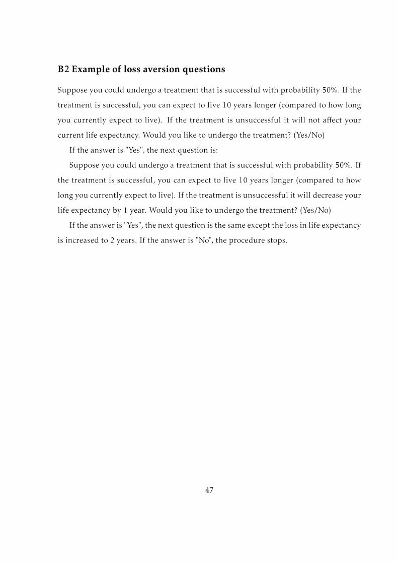
B2 Example of loss aversion questions

Suppose you could undergo a treatment that is successful with probability 50%. If the

treatment is successful, you can expect to live 10 years longer (compared to how long

you currently expect to live). If the treatment is unsuccessful it will not affect your

current life expectancy. Would you like to undergo the treatment? (Yes/No)

If the answer is "Yes", the next question is:

Suppose you could undergo a treatment that is successful with probability 50%. If

the treatment is successful, you can expect to live 10 years longer (compared to how

long you currently expect to live). If the treatment is unsuccessful it will decrease your

life expectancy by 1 year. Would you like to undergo the treatment? (Yes/No)

If the answer is "Yes", the next question is the same except the loss in life expectancy

is increased to 2 years. If the answer is "No", the procedure stops.

47

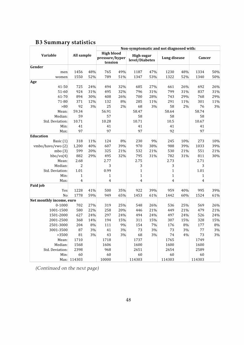
B3 Summary statistics

Variable All sample

Non-symptomatic and not diagnosed with:

Lung disease Cancer

Gender men 1456 48% 765 49% 1187 47% 1230 48% 1334 50%women 1550 52% 789 51% 1347 53% 1322 52% 1340 50%Age 41-50 725 24% 494 32% 685 27% 661 26% 692 26%51-60 924 31% 495 32% 796 31% 799 31% 837 31%61-70 894 30% 408 26% 700 28% 743 29% 768 29%71-80 371 12% 132 8% 285 11% 291 11% 301 11%>80 92 3% 25 2% 68 3% 58 2% 76 3%Mean: 59.34 56.91 58.47 58.64 58.74Median: 59 57 58 58 5810.71 10.28 10.71 10.5 10.67Min: 41 41 41 41 41Max: 97 97 97 92 97Education Basic (1) 318 11% 124 8% 230 9% 245 10% 273 10%1,200 40% 607 39% 970 38% 988 39% 1033 39%599 20% 325 21% 532 21% 530 21% 551 21%882 29% 495 32% 795 31% 782 31% 811 30%Mean: 2.68 2.77 2.75 2.73 2.71Median: 2 3 3 3 31.01 0.99 1 1 1.01Min: 1 1 1 1 1Max: 4 4 4 4 4Paid job Yes 1228 41% 500 35% 922 39% 959 40% 995 39%No 1778 59% 949 65% 1453 61% 1442 60% 1524 61%0-1000 702 27% 319 25% 548 26% 536 25% 569 26%1001-1500 580 22% 258 20% 446 21% 449 21% 479 21%1501-2000 627 24% 297 24% 494 24% 497 24% 526 24%2001-2500 368 14% 194 15% 311 15% 307 15% 328 15%2501-3000 204 8% 111 9% 154 7% 176 8% 177 8%3001-3500 87 3% 41 3% 73 3% 73 3% 77 3%>3500 81 3% 43 3% 68 3% 74 4% 73 3%Mean: 1710 1718 1737 1765 1749Median: 1568 1606 1600 1600 16002398 968 2651 2654 2589Min: 60 60 60 60 60Max: 114303 10000 114303 114303 114303

High blood pressure/hyper

tension

High sugar level/Diabetes

Std. Deviation:vmbo/havo/vwo (2)mbo (3)hbo/vo(4)

Std. Deviation:

Net monthly income, euro

Std. Deviation:(Continued on the next page)

48

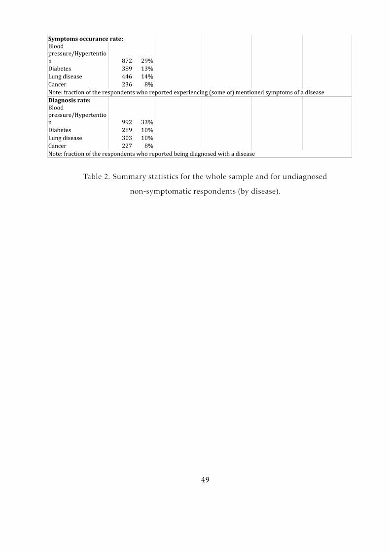
872 29%Diabetes 389 13%Lung disease 446 14%Cancer 236 8%Note: fraction of the respondents who reported experiencing (some of) mentioned symptoms of a diseaseDiagnosis rate:

992 33%Diabetes 289 10%Lung disease 303 10%Cancer 227 8%Note: fraction of the respondents who reported being diagnosed with a disease

Symptoms occurance rate:Blood pressure/Hypertention

Blood pressure/Hypertention

Table 2. Summary statistics for the whole sample and for undiagnosed

non-symptomatic respondents (by disease).

49

B4 Loss aversion values

Loss aversion Number of respondents % of the sample1 58 3 947 31.502 20 1 830 27.613 6.67 0.298 356 11.844 4.00 0.158 303 10.085 2.86 0.098 187 6.226 2.22 0.064 121 4.037 1.82 0.043 97 3.238 1.54 0.028 30 1.009 1.33 0.018 12 0.4010 1.18 0.009 15 0.5011 1.05 0.003 15 0.50All “yes” 1.00 0 93 3.09Mean: 25.38 1.28Median: 20 123.11 1.21

Index of rejected lottery

Loss aversion (normalized)

Std. deviation:Table 3. Distribution of loss aversion values.

B5 Distribution of testing frequencies

Blood pressure testingAll respondents Undiagnosed non-symptomaticN. % N. %Never 747 24.91 541 36.11Once a year 878 29.28 548 36.582 times a year 397 13.24 163 10.883-4 times a year 543 18.11 148 9.88Once in 2 months 168 5.60 48 3.20Once a month 140 4.67 26 1.742-3 times a month 78 2.60 18 1.20Once a week or more 48 1.60 6 0.40Total: 2999* 100 1498 100*Note: 7 observations are missing from the original sample due to non-response

   Frequency of tests

Table 4. Distribution of blood pressure test frequency.

50

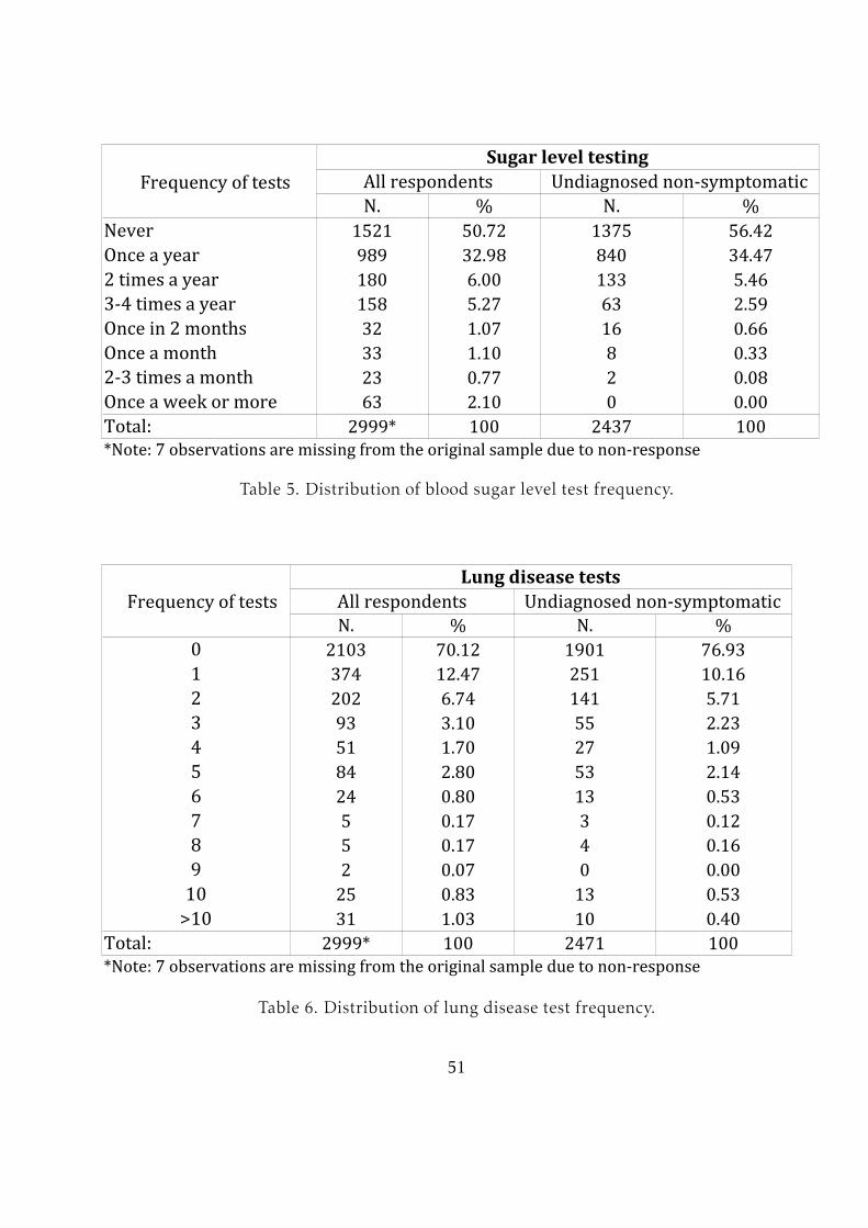
Sugar level testingAll respondents Undiagnosed non-symptomaticN. % N. %Never 1521 50.72 1375 56.42Once a year 989 32.98 840 34.472 times a year 180 6.00 133 5.463-4 times a year 158 5.27 63 2.59Once in 2 months 32 1.07 16 0.66Once a month 33 1.10 8 0.332-3 times a month 23 0.77 2 0.08Once a week or more 63 2.10 0 0.00Total: 2999* 100 2437 100*Note: 7 observations are missing from the original sample due to non-response

   Frequency of tests

Table 5. Distribution of blood sugar level test frequency.

Lung disease testsAll respondents Undiagnosed non-symptomaticN. % N. %0 2103 70.12 1901 76.931 374 12.47 251 10.162 202 6.74 141 5.713 93 3.10 55 2.234 51 1.70 27 1.095 84 2.80 53 2.146 24 0.80 13 0.537 5 0.17 3 0.128 5 0.17 4 0.169 2 0.07 0 0.0010 25 0.83 13 0.53>10 31 1.03 10 0.40Total: 2999* 100 2471 100*Note: 7 observations are missing from the original sample due to non-response

   Frequency of tests

Table 6. Distribution of lung disease test frequency.

51

Medical tests for cancerAll respondents Undiagnosed non-symptomaticmen women men womenN. % N. % N. % N. %0 1191 82.02 922 59.6 1124 86.59 848 65.481 105 7.23 170 10.99 84 6.47 134 10.352 50 3.44 113 7.3 35 2.7 85 6.563 17 1.17 65 4.2 14 1.08 47 3.634 12 0.83 49 3.17 9 0.69 37 2.865 16 1.1 121 7.82 12 0.92 97 7.496 10 0.69 15 0.97 5 0.39 9 0.697 6 0.41 6 0.39 2 0.15 4 0.318 5 0.34 18 1.16 1 0.08 10 0.779 1 0.07 3 0.19 1 0.08 2 0.1510 12 0.83 37 2.39 7 0.54 14 1.08>10 27 1.88 28 1.8 4 0.32 8 0.62Total: 1452 100 1547 100 1298 100 1295 100Note: 7 observations are missing from the original sample due to non-response

   Frequency of tests

Table 7. Distribution of cancer test frequency.

Self-test for cancerAll respondents Undiagnosed non-symptomaticmen women men womenN. % N. % N. % N. %Never 1230 84.71 544 35.16 1125 86.67 479 36.99Once a year 139 9.57 278 17.97 119 9.17 242 18.692 times a year 36 2.48 119 7.69 26 2.00 97 7.493-4 times a year 16 1.10 184 11.89 6 0.46 154 11.89Once in 2 months 5 0.34 118 7.63 4 0.31 92 7.10Once a month 15 1.03 205 13.25 9 0.69 159 12.282-3 times a month 4 0.28 53 3.43 3 0.23 38 2.93Once a week or more 7 0.48 46 2.97 6 0.46 34 2.63Total: 1452 100 1547 100 1298 100 1295 100Note: 7 observations are missing from the original sample due to non-response

   Frequency of tests

Table 8. Distribution of cancer self-test frequency.

52

B6 Estimation results

Blood pressure testsSample: Excludes loss aversion group 12 Excludes loss aversion group 12Dependent variable : Decision to test (binary) Frequency of tests (categorical)Log of loss aversion -0.048** -0.049** -0.050 -0.050(0.024) (0.024) (0.041) (0.041)Gender -0.098 -0.291** -0.32**(0.075) (0.140) (0.138)Age 0.018*** 0.016*** 0.028*** 0.021***(0.005) (0.004) (0.009) (0.007)0.051 0.061* 0.029 0.033(0.038) (0.037) (0.069) (0.066)Paid job 0.104 0.266(0.093) (0.171)Long-stand. disease 0.061 0.175(0.088) (0.149)BMI 0.022*** 0.024*** 0.012 0.013(0.010) (0.010) (0.020) (0.019)Smoking -0.13** -0.118* 0.028(0.064) (0.064) (0.127)Alcohol -0.025 -0.03* 0.001(0.017) (0.017) (0.032)0.105*** 0.105*** 0.059** 0.074***(0.022) (0.020) (0.035) (0.031)0.009 0.020(0.024) (0.039)Worry 0.277*** 0.278*** 0.182 0.189*(0.066) (0.065) (0.115) (0.112)Family history 0.133* 0.122* 0.166 0.159(0.073) (0.073) (0.138) (0.137)Regression type:N. of observations: 1440 1440 920 9200.000 0.000 0.000 0.000Pseudo R-squared: 0.06 0.06 0.017 0.015Notes: sample consists of undiagnosed non-symptomatic people.Significance: * - at 10% level, ** - at 5% level, *** - at 1% level; robust standard errors in parentheses.Loss aversion group 12 contains individuals who responded “Yes” to all lottery questions.

Edu

Fam. physicianMed. specialistprobit probit ordered logit ordered logitLR-test (prob.>chi^2):

Table 9. Estimation results for two-part model: blood pressure tests.

53

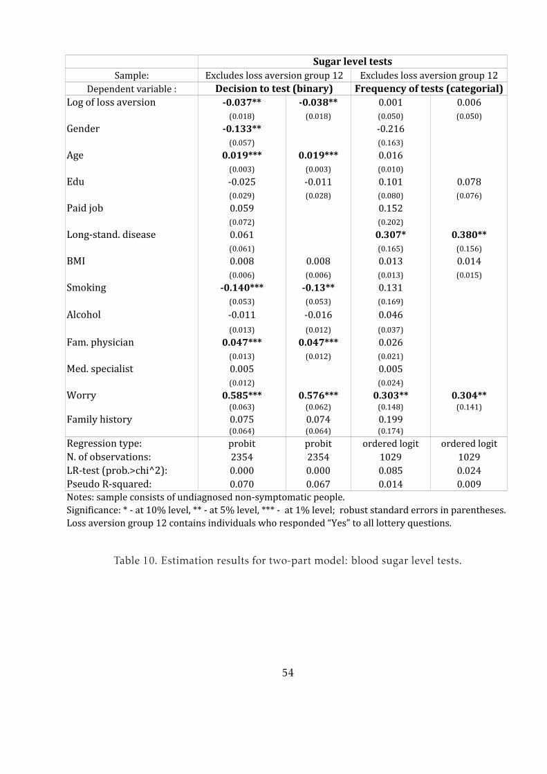
Sugar level testsSample: Excludes loss aversion group 12 Excludes loss aversion group 12Dependent variable : Decision to test (binary)Log of loss aversion -0.037** -0.038** 0.001 0.006(0.018) (0.018) (0.050) (0.050)Gender -0.133** -0.216(0.057) (0.163)Age 0.019*** 0.019*** 0.016(0.003) (0.003) (0.010)-0.025 -0.011 0.101 0.078(0.029) (0.028) (0.080) (0.076)Paid job 0.059 0.152(0.072) (0.202)Long-stand. disease 0.061 0.307* 0.380**(0.061) (0.165) (0.156)BMI 0.008 0.008 0.013 0.014(0.006) (0.006) (0.013) (0.015)Smoking -0.140*** -0.13** 0.131(0.053) (0.053) (0.169)Alcohol -0.011 -0.016 0.046(0.013) (0.012) (0.037)0.047*** 0.047*** 0.026(0.013) (0.012) (0.021)0.005 0.005(0.012) (0.024)Worry 0.585*** 0.576*** 0.303** 0.304**(0.063) (0.062) (0.148) (0.141)Family history 0.075 0.074 0.199(0.064) (0.064) (0.174)Regression type:N. of observations: 2354 2354 1029 10290.000 0.000 0.085 0.024Pseudo R-squared: 0.070 0.067 0.014 0.009Notes: sample consists of undiagnosed non-symptomatic people.Significance: * - at 10% level, ** - at 5% level, *** - at 1% level; robust standard errors in parentheses.Loss aversion group 12 contains individuals who responded “Yes” to all lottery questions.

Frequency of tests (categorial)

Edu

Fam. physicianMed. specialist

probit probit ordered logit ordered logitLR-test (prob.>chi^2):

Table 10. Estimation results for two-part model: blood sugar level tests.

54

Lung disease testsSample: Excludes loss aversion group 12 Excludes loss aversion group 12Dependent variable : Decision to test (binary) Frequency of tests (continuous)Log of loss aversion -0.052*** -0.052*** -0.035 -0.048(0.020) (0.020) (0.073) (0.076)Gender 0.108* 0.100* 0.859*** 0.769***(0.061) (0.060) (0.230) (0.236)Age 0.016*** 0.016*** 0.017 0.017(0.003) (0.003) (0.013) (0.013)-0.067** -0.070** -0.101(0.031) (0.030) (0.120)BMI 0.007 0.013(0.006) (0.027)Smoking 0.093 0.090 0.184(0.061) (0.061) (0.243)Alcohol -0.005 -0.075(0.013) (0.054)Worry 0.239*** 0.248*** -0.077(0.070) (0.070) (0.050)Family history 0.102 -0.482* -0.470**(0.077) (0.258) (0.243)Flu frequency 0.128*** 0.128*** 0.146(0.026) (0.026) (0.120)Flu shots 0.051** 0.053*** 0.126* 0.120*(0.015) (0.015) (0.069) (0.069)Immunity -0.189** -0.198** 0.325(0.089) (0.088) (0.330)Regression type: OLS OLSN. of observations: 2384 2384 554 5540.000 0.000(Pseudo) R-squared: 0.064 0.063 0.057 0.043Notes: sample consists of undiagnosed non-symptomatic people.Significance: * - at 10% level, ** - at 5% level, *** - at 1% level; robust standard errors in parentheses.Loss aversion group 12 contains individuals who responded “Yes” to all lottery questions.

Edu

probit probitLR-test (prob.>chi^2): 0.000(1) 0.000(1)

(1) F-test for OLS regressionTable 11. Estimation results for two-part model: lung disease tests.

55

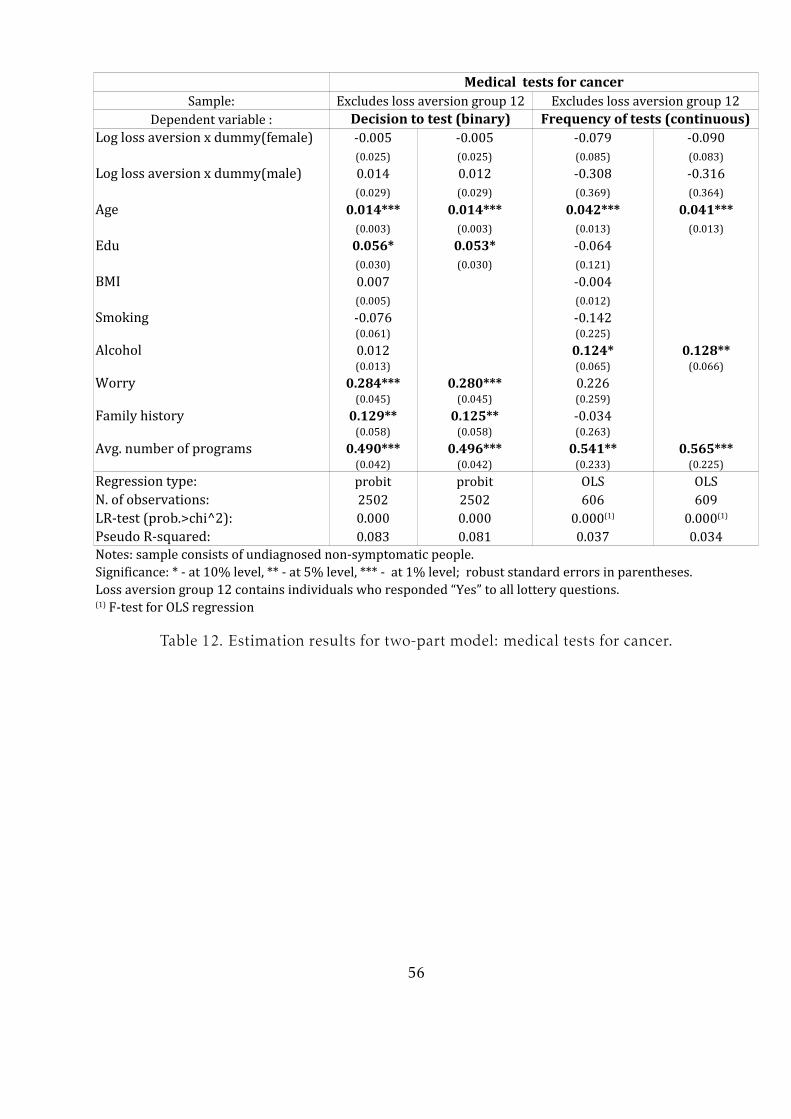
Medical tests for cancerSample: Excludes loss aversion group 12 Excludes loss aversion group 12Dependent variable : Decision to test (binary) Frequency of tests (continuous)Log loss aversion x dummy(female) -0.005 -0.005 -0.079 -0.090(0.025) (0.025) (0.085) (0.083)Log loss aversion x dummy(male) 0.014 0.012 -0.308 -0.316(0.029) (0.029) (0.369) (0.364)Age 0.014*** 0.014*** 0.042*** 0.041***(0.003) (0.003) (0.013) (0.013)0.056* 0.053* -0.064(0.030) (0.030) (0.121)BMI 0.007 -0.004(0.005) (0.012)Smoking -0.076 -0.142(0.061) (0.225)Alcohol 0.012 0.124* 0.128**(0.013) (0.065) (0.066)Worry 0.284*** 0.280*** 0.226(0.045) (0.045) (0.259)Family history 0.129** 0.125** -0.034(0.058) (0.058) (0.263)

0.490*** 0.496*** 0.541** 0.565***(0.042) (0.042) (0.233) (0.225)Regression type: OLS OLSN. of observations: 2502 2502 606 6090.000 0.000Pseudo R-squared: 0.083 0.081 0.037 0.034Notes: sample consists of undiagnosed non-symptomatic people.Significance: * - at 10% level, ** - at 5% level, *** - at 1% level; robust standard errors in parentheses.Loss aversion group 12 contains individuals who responded “Yes” to all lottery questions.

Edu

Avg. number of programs probit probitLR-test (prob.>chi^2): 0.000(1) 0.000(1)

(1) F-test for OLS regressionTable 12. Estimation results for two-part model: medical tests for cancer.

56

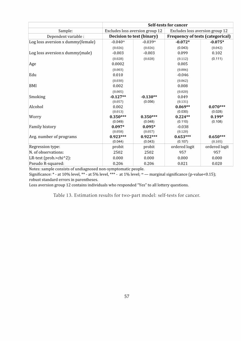
Self-tests for cancerSample: Excludes loss aversion group 12 Excludes loss aversion group 12Dependent variable : Decision to test (binary) Frequency of tests (categorical)Log loss aversion x dummy(female) -0.072* -0.075*(0.026) (0.026) (0.043) (0.042)-0.003 -0.003 0.099 0.102(0.028) (0.028) (0.112) (0.111)Age 0.0002 0.005(0.003) (0.006)0.010 -0.046(0.030) (0.062)BMI 0.002 0.008(0.005) (0.020)Smoking -0.127** -0.130** 0.049(0.057) (0.056) (0.131)Alcohol 0.002 0.069** 0.070***(0.013) (0.030) (0.028)Worry 0.350*** 0.350*** 0.224** 0.199*(0.049) (0.048) (0.110) (0.108)Family history 0.097* 0.095* -0.038(0.058) (0.057) (0.120)

0.923*** 0.922*** 0.653*** 0.650***(0.044) (0.043) (0.107) (0.105)Regression type:N. of observations: 2502 2502 957 9570.000 0.000 0.000 0.000Pseudo R-squared: 0.206 0.206 0.021 0.020Notes: sample consists of undiagnosed non-symptomatic people.robust standard errors in parentheses.Loss aversion group 12 contains individuals who responded “Yes” to all lottery questions.

-0.040m -0.039mLog loss aversion x dummy(male)Edu

Avg. number of programs probit probit ordered logit ordered logitLR-test (prob.>chi^2):Significance: * - at 10% level, ** - at 5% level, *** - at 1% level; m — marginal significance (p-value<0.15);

Table 13. Estimation results for two-part model: self-tests for cancer.

57

Blood pressure tests: robustness checkSample: Excludes loss aversion group 1 Includes loss aversion group 12Dependent variable : Decision to test (binary) Decision to test (binary)-0.062* -0.059* -0.043*(0.036) (0.036) (0.026) (0.026)Gender -0.059 -0.083 -0.101(0.094) (0.074) (0.073)Age 0.018*** 0.017*** 0.018*** 0.016***(0.006) (0.005) (0.005) (0.004)0.094** 0.099** 0.050 0.052(0.047) (0.047) (0.037) (0.037)Paid job 0.051 0.104(0.117) (0.092)Long-stand. disease 0.109 -0.066(0.107) (0.085)BMI 0.034*** 0.035*** 0.021** 0.022**(0.012) (0.013) (0.010) (0.010)Smoking -0.147* -0.138* -0.138** -0.135**(0.081) (0.081) (0.062) (0.062)Alcohol -0.014 -0.017 -0.027* -0.028*(0.021) (0.021) (0.016) (0.016)

0.111*** 0.109*** 0.101*** 0.110***(0.027) (0.024) (0.021) (0.020)-0.009 0.017(0.022) (0.021)Worry 0.235*** 0.234*** 0.291*** 0.294***(0.078) (0.076) (0.065) (0.065)Family history 0.177** 0.172**(0.091) (0.090) (0.072) (0.072)Regression type:N. of observations: 957 957 1492 14920.000 0.000 0.000 0.000Pseudo R-squared: 0.06 0.06 0.065 0.063Notes: sample consists of undiagnosed non-symptomatic people.Significance: * - at 10% level, ** - at 5% level, *** - at 1% level; m – indicates marginal significance(p-value<0.15); robust standard errors in parentheses.in columns 3 and 4 regressions contain natural log of non-normalized loss aversion in order to include loss aversion of 1 that becomes zero in case of normalization.Loss aversion group 12 contains individuals who accepted all lotteries (loss neutral).Loss aversion group 1 contains individuals who rejected 'harmless' lottery (extremely loss averse).

Loss aversion(1) -0.042m

Edu

Fam. physicianMed. specialist0.113m 0.112m

probit probit probit probitLR-test (prob.>chi^2):(1) In columns 1 and 2 regressions contain natural log of normalized loss aversion;

Table 14. Robustness checks for high blood pressure/hypertension testing.

58

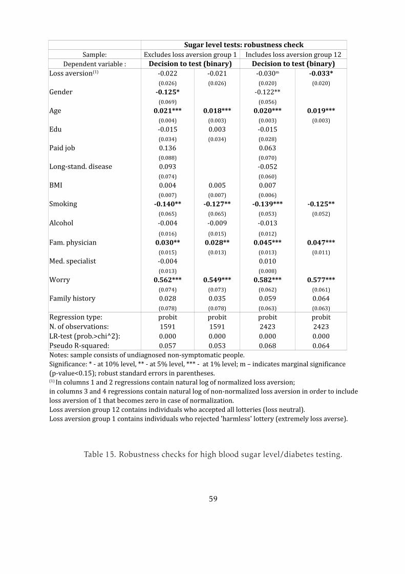
Sugar level tests: robustness checkSample: Excludes loss aversion group 1 Includes loss aversion group 12Dependent variable : Decision to test (binary) Decision to test (binary)-0.022 -0.021 -0.033*(0.026) (0.026) (0.020) (0.020)Gender -0.125* -0.122**(0.069) (0.056)Age 0.021*** 0.018*** 0.020*** 0.019***(0.004) (0.003) (0.003) (0.003)-0.015 0.003 -0.015(0.034) (0.034) (0.028)Paid job 0.136 0.063(0.088) (0.070)Long-stand. disease 0.093 -0.052(0.074) (0.060)BMI 0.004 0.005 0.007(0.007) (0.007) (0.006)Smoking -0.140** -0.127** -0.139*** -0.125**(0.065) (0.065) (0.053) (0.052)Alcohol -0.004 -0.009 -0.013(0.016) (0.015) (0.012)0.030** 0.028** 0.045*** 0.047***(0.015) (0.013) (0.013) (0.011)-0.004 0.010(0.013) (0.008)Worry 0.562*** 0.549*** 0.582*** 0.577***(0.074) (0.073) (0.062) (0.061)Family history 0.028 0.035 0.059 0.064(0.078) (0.078) (0.063) (0.063)Regression type:N. of observations: 1591 1591 2423 24230.000 0.000 0.000 0.000Pseudo R-squared: 0.057 0.053 0.068 0.064Notes: sample consists of undiagnosed non-symptomatic people.Significance: * - at 10% level, ** - at 5% level, *** - at 1% level; m – indicates marginal significance(p-value<0.15); robust standard errors in parentheses.in columns 3 and 4 regressions contain natural log of non-normalized loss aversion in order to include loss aversion of 1 that becomes zero in case of normalization.Loss aversion group 12 contains individuals who accepted all lotteries (loss neutral).Loss aversion group 1 contains individuals who rejected 'harmless' lottery (extremely loss averse).

Loss aversion(1) -0.030m

Edu

Fam. physicianMed. specialist

probit probit probit probitLR-test (prob.>chi^2):(1) In columns 1 and 2 regressions contain natural log of normalized loss aversion;

Table 15. Robustness checks for high blood sugar level/diabetes testing.

59

Lung disease tests: robustness checkSample: Excludes loss aversion group 1 Includes loss aversion group 12Dependent variable : Decision to test (binary) Decision to test (binary)-0.069** -0.065** -0.043** -0.040*(0.029) (0.029) (0.022) (0.022)Gender 0.142** 0.125* 0.119** 0.107*(0.075) (0.074) (0.060) (0.059)Age 0.016*** 0.017*** 0.016*** 0.015***(0.004) (0.004) (0.003) (0.003)-0.058* -0.053 -0.067** -0.077***(0.037) (0.036) (0.030) (0.029)BMI 0.02** 0.018** 0.006(0.009) (0.009) (0.005)Smoking 0.130* 0.129* 0.095(0.074) (0.074) (0.059)Alcohol -0.020 -0.005(0.017) (0.013)Worry 0.204** 0.221*** 0.228*** 0.259***(0.084) (0.084) (0.069) (0.066)Family history 0.133 0.144 0.088(0.095) (0.094) (0.077)Flu frequency 0.127*** 0.129*** 0.123*** 0.123***(0.034) (0.034) (0.025) (0.025)Flu shots 0.059*** 0.059*** 0.051*** 0.050***(0.019) (0.019) (0.014) (0.014)Immunity -0.149 -0.159* -0.165*(0.108) (0.088) (0.087)Regression type:N. of observations: 1599 1599 2461 24610.000 0.000 0.000 0.000Pseudo R-squared: 0.069 0.067 0.061 0.059Notes: sample consists of undiagnosed non-symptomatic people.Significance: * - at 10% level, ** - at 5% level, *** - at 1% level; m – indicates marginal significance(p-value<0.15); robust standard errors in parentheses.in columns 3 and 4 regressions contain natural log of non-normalized loss aversion in order to include loss aversion of 1 that becomes zero in case of normalization.Loss aversion group 12 contains individuals who accepted all lotteries (loss neutral).Loss aversion group 1 contains individuals who rejected 'harmless' lottery (extremely loss averse).

Loss aversion(1)

Edu

probit probit probit probitLR-test (prob.>chi^2):(1) In columns 1 and 2 regressions contain natural log of normalized loss aversion;

Table 16. Robustness checks for lung disease testing.

60

Self-tests for cancer: robustness checkSample: Excludes loss aversion group 1 Includes loss aversion group 12Dependent variable : Frequency of tests(categorical) Frequency of tests(categorical)-0.004 -0.009 0.007 0.005(0.061) (0.061) (0.048) (0.047)0.399** 0.387** -0.493*** -0.491***(0.175) (0.174) (0.102) (0.102)Age -0.003 0.006(0.008) (0.006)-0.039 -0.012(0.073) (0.062)BMI 0.023 0.006(0.018) (0.017)Smoking 0.103 0.109(0.154) (0.132)Alcohol 0.067** 0.079** 0.054* 0.052**(0.036) (0.035) (0.029) (0.028)Worry 0.180 0.208* 0.194*(0.137) (0.134) (0.111) (0.109)Family history -0.102 -0.103 0.027(0.143) (0.141) (0.119)

0.516*** 0.523*** 0.106 0.104(0.156) (0.156) (0.139) (0.138)Regression type:N. of observations: 661 661 985 9850.000 0.000 0.000 0.000Pseudo R-squared: 0.027 0.023 0.028 0.027Notes: sample consists of undiagnosed non-symptomatic people.(p-value<0.15); robust standard errors in parentheses.in columns 3 and 4 regressions contain natural log of non-normalized loss aversion in order to include loss aversion of 1 that becomes zero in case of normalization.Loss aversion group 12 contains individuals who accepted all lotteries (loss neutral).Loss aversion group 1 contains individuals who rejected 'harmless' lottery (extremely loss averse).

Loss aversion(1) x dummy(female)Loss aversion(1) x dummy(male)Edu

0.198m

Avg. number of programs ordered logit ordered logit ordered logit ordered logitLR-test (prob.>chi^2):Significance: * - at 10% level, ** - at 5% level, *** - at 1% level; m – indicates marginal significance(1) In columns 1 and 2 regressions contain natural log of normalized loss aversion;

Table 17. Robustness checks for self-tests for cancer.

61

B7 Marginal effects

Marginal effects for:Blood pressure testingUnitary change Unitary changeLog of loss aversion 0.0183 0.0271 0.0123 0.0187Gender 0.0779 0.0390Age -0.0058 -0.0595 -0.0050 -0.0517-0.0225 -0.0223 -0.0081 -0.0081Paid jobLong-stand. diseaseBMI -0.0087 -0.0428 -0.0032 -0.0171Smoking 0.0436 0.0236Alcohol 0.0109 0.0247-0.0388 -0.0946 -0.0180 -0.0493

Worry -0.1027 -0.0601 -0.0460 -0.0284Family history -0.0449 -0.0217 -0.0388 -0.0187Predicted outcome: Never test Never test Once a year Once a yearPredicted probability: 0.3478 0.3478 0.5779 0.5779N. of observations: 1440 1440 920 920

Participation (probit) Frequency (ordered logit)1 std. dev. 1 std. dev.

Edu

Fam. physicianMed. specialist

Note: columns 1 and 3 show marginal effects (i.e. an absolute change in the predicted probability of a given outcome) for an increase of regressor by 1 (for continuous variables) or a change of regressor from 0 to 1 (for binary variables). Columns 2 and 4 show marginal effects when a regressor changes by one standard deviation. Marginal effects are estimated given the mean values of variables. Table 18. Marginal effects: blood pressure tests.

62

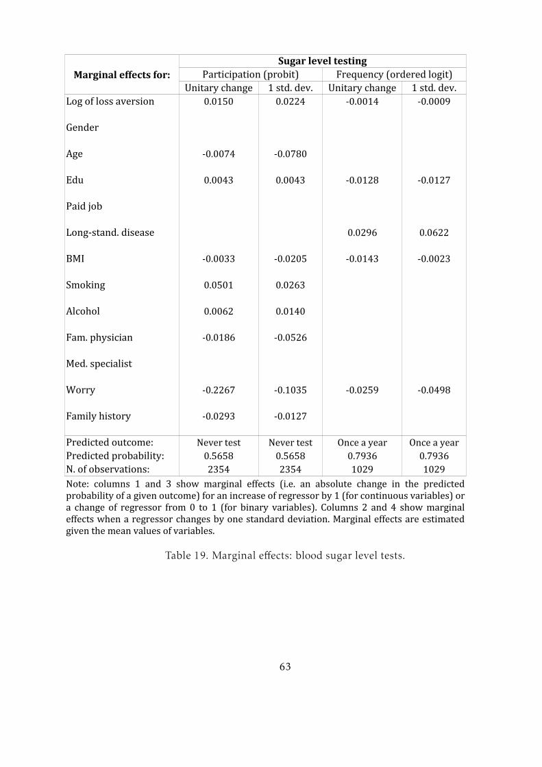
Marginal effects for:Sugar level testingUnitary change Unitary changeLog of loss aversion 0.0150 0.0224 -0.0014 -0.0009GenderAge -0.0074 -0.07800.0043 0.0043 -0.0128 -0.0127Paid jobLong-stand. disease 0.0296 0.0622BMI -0.0033 -0.0205 -0.0143 -0.0023Smoking 0.0501 0.0263Alcohol 0.0062 0.0140-0.0186 -0.0526

Worry -0.2267 -0.1035 -0.0259 -0.0498Family history -0.0293 -0.0127Predicted outcome: Never test Never test Once a year Once a yearPredicted probability: 0.5658 0.5658 0.7936 0.7936N. of observations: 2354 2354 1029 1029

Participation (probit) Frequency (ordered logit)1 std. dev. 1 std. dev.

Edu

Fam. physicianMed. specialist

Note: columns 1 and 3 show marginal effects (i.e. an absolute change in the predicted probability of a given outcome) for an increase of regressor by 1 (for continuous variables) or a change of regressor from 0 to 1 (for binary variables). Columns 2 and 4 show marginal effects when a regressor changes by one standard deviation. Marginal effects are estimated given the mean values of variables.Table 19. Marginal effects: blood sugar level tests.

63

Marginal effects for:Lung disease testingFrequency (OLS)Unitary change Unitary changeLog of loss aversion 0.0152 0.0224 -0.0353 -0.0550Gender -0.0296 -0.0148 0.8557 0.4265Age -0.0047 -0.0494 0.0191 0.18900.0207 0.0208BMISmoking -0.0266 -0.0135Alcohol -0.0663 -0.1547Worry -0.0734 -0.0303Family history -0.4593 -0.1828Flu frequency -0.0379 -0.0543 0.1435 0.2611Flu shots -0.0157 -0.0358 0.1220 0.3048Immunity 0.0586 0.0187 0.3479 0.1279Predicted outcome: Never test Never testPredicted probability: 0.7808 0.7808N. of observations: 2384 2384 554 554

Participation (probit)1 std. dev. 1 std. dev.

Edu

2.641 2.641

Note: in the first column marginal effects represent absolute change in the predicted probability of outcome given an increase of regressor by 1 (for continuous variables) or a change of regressor from 0 to 1 (for binary variables). In the third column marginal effects represent absolute change in the number of tests during 10 years given a unitary change in regressor. Columns 2 and 4 show marginal effects when a regressor changes by one standard deviation. Marginal effects are estimated given the mean values of regressors.1Predicted number of tests during 10 years given the mean values of regressors.Table 20. Marginal effects: lung disease tests.

64

Marginal effects for:Medical tests for cancerFrequency (OLS)Unitary change Unitary changeLog loss aversion x dummy (female) 0.0014 0.0015 -0.0903 -0.1141Log loss aversion x dummy (male) -0.0035 -0.0037 -0.3159 -0.2511Age -0.0041 -0.0436 0.0415 0.4011-0.0157 -0.0159BMISmokingAlcohol 0.1280 0.2986Worry -0.0834 -0.0541Family history -0.0372 -0.0186-0.1480 -0.1032 0.5556 0.3775Predicted outcome: Never test Never testPredicted probability: 0.7778 0.7778N. of observations: 2502 2502 606 606

Participation (probit)1 std. dev. 1 std. dev.

Edu

Avg. number of programs 3.271 3.271

Note: in the first column marginal effects represent absolute change in the predicted probability of outcome given an increase of regressor by 1 (for continuous variables) or a change of regressor from 0 to 1 (for binary variables). In the third column marginal effects represent absolute change in the number of tests during 10 years given a unitary change in regressor. Marginal effects are estimated given the mean values of regressors. Columns 2 and 4 show marginal effects when a regressor changes by one standard deviation. 1Predicted number of tests during 10 years given the mean values of regressors.Table 21. Marginal effects: medical tests for cancer.

65

Marginal effects for:Self-tests for cancerUnitary change Unitary changeLoss aversion x dummy(female) 0.0147 0.0158 0.0173 0.0240Loss aversion x dummy(male) 0.0012 0.0013 -0.0233 -0.0155Age

BMISmoking 0.0485 0.0252Alcohol -0.0160 -0.0358Worry -0.1307 -0.0845 -0.0455 -0.0286Family history -0.0355 -0.0177-0.3439 -0.2367 -0.1490 -0.0909Predicted outcome: Never test Never test Once a year Once a yearPredicted probability: 0.6436 0.6436 0.3555 0.3555N. of observations: 2502 2502 957 957

Participation (probit) Frequency (ordered logit)1 std. dev. 1 std. dev.

Edu

Avg. number of programsNote: marginal effects represent absolute change in the predicted probability of outcome given an increase of regressor by 1 (for continuous variables) or a change of regressor from 0 to 1 (for binary variables). Columns 2 and 4 show marginal effects when a regressor changes by one standard deviation. Marginal effects are estimated given the mean values of regressors.

Table 22. Marginal effects: self-tests for cancer.

66

Predicted probability of participation in testingBlood pressure test Sugar level test Lung disease test1 1.1 0.624 0.410 0.2 0.3352 0 0.644 0.427 0.215 0.3543 -1.21 0.666 0.446 0.232 0.3764 -1.85 0.678 0.455 0.241 0.3885 -2.33 0.686 0.463 0.248 0.3976 -2.74 0.693 0.470 0.255 0.4057 -3.15 0.700 0.476 0.261 0.4128 -3.56 0.708 0.482 0.267 0.4209 -4.04 0.716 0.490 0.274 0.42910 -4.68 0.726 0.500 0.284 0.44111 -5.89 0.746 0.519 0.304 0.465All “yes” -Average change: 0.0122 0.0109 0.0103 0.0130

Index of rejected lottery Ln(loss aversion) Self-test for cancer

(women)

Note: Table shows predicted probability of participation in testing given each value of loss aversion and mean values of all other variables. Results for cancer screening are not provided since loss aversion is not significant for participation decision.Table 23. Predicted probabilities of participation in testing.

67

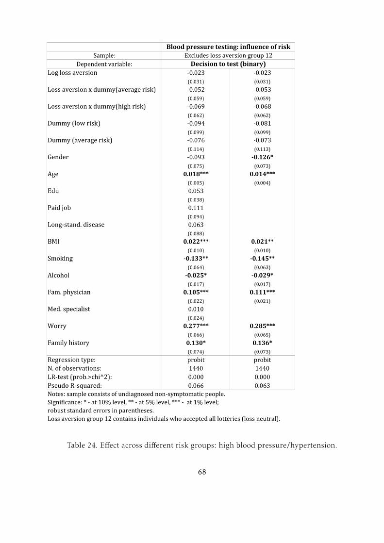
Blood pressure testing: influence of riskSample: Excludes loss aversion group 12Dependent variable: Decision to test (binary)Log loss aversion -0.023 -0.023(0.031) (0.031)Loss aversion x dummy(average risk) -0.052 -0.053(0.059) (0.059)Loss aversion x dummy(high risk) -0.069 -0.068(0.062) (0.062)Dummy (low risk) -0.094 -0.081(0.099) (0.099)Dummy (average risk) -0.076 -0.073(0.114) (0.113)Gender -0.093 -0.126*(0.075) (0.073)Age 0.018*** 0.014***(0.005) (0.004)0.053(0.038)Paid job 0.111(0.094)Long-stand. disease 0.063(0.088)BMI 0.022*** 0.021**(0.010) (0.010)Smoking -0.133** -0.145**(0.064) (0.063)Alcohol -0.025* -0.029*(0.017) (0.017)0.105*** 0.111***(0.022) (0.021)0.010(0.024)Worry 0.277*** 0.285***(0.066) (0.065)Family history 0.130* 0.136*(0.074) (0.073)Regression type:N. of observations: 1440 14400.000 0.000Pseudo R-squared: 0.066 0.063Notes: sample consists of undiagnosed non-symptomatic people.Significance: * - at 10% level, ** - at 5% level, *** - at 1% level; robust standard errors in parentheses.Loss aversion group 12 contains individuals who accepted all lotteries (loss neutral).

Edu

Fam. physicianMed. specialist

probit probitLR-test (prob.>chi^2):

Table 24. Effect across different risk groups: high blood pressure/hypertension.

68

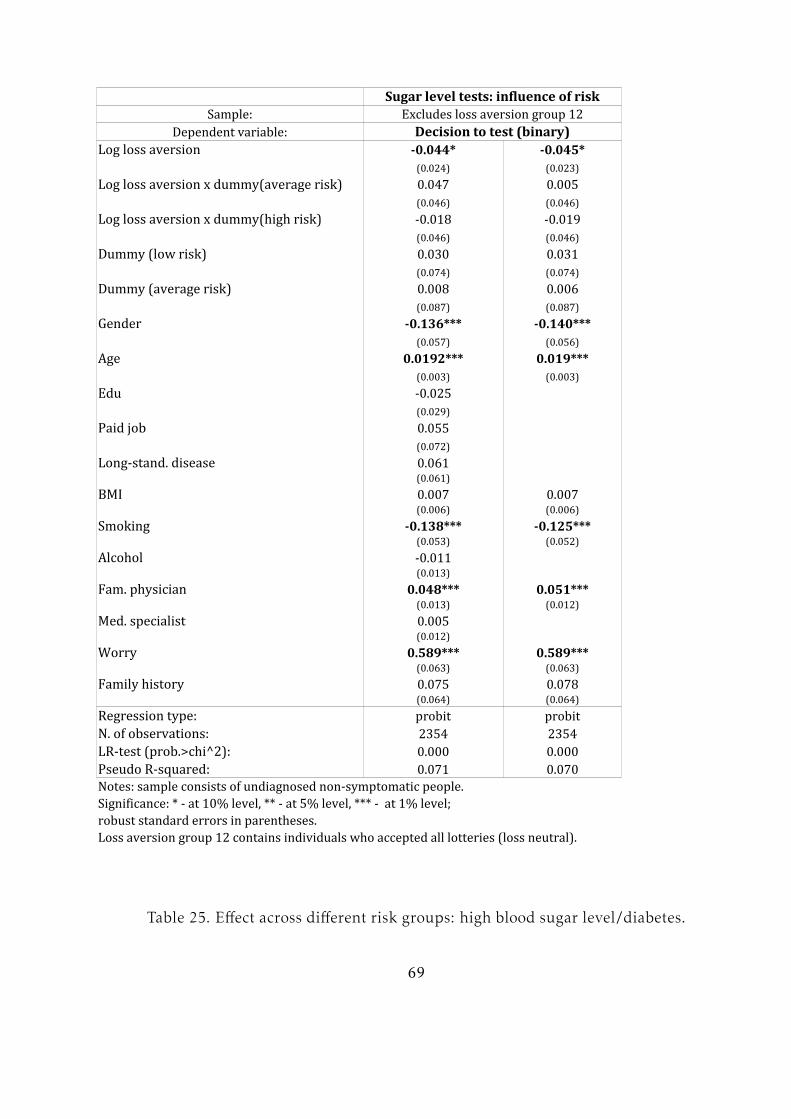
Sugar level tests: influence of riskSample: Excludes loss aversion group 12Dependent variable: Decision to test (binary)Log loss aversion -0.044* -0.045*(0.024) (0.023)Log loss aversion x dummy(average risk) 0.047 0.005(0.046) (0.046)Log loss aversion x dummy(high risk) -0.018 -0.019(0.046) (0.046)Dummy (low risk) 0.030 0.031(0.074) (0.074)Dummy (average risk) 0.008 0.006(0.087) (0.087)Gender -0.136*** -0.140***(0.057) (0.056)Age 0.0192*** 0.019***(0.003) (0.003)-0.025(0.029)Paid job 0.055(0.072)Long-stand. disease 0.061(0.061)BMI 0.007 0.007(0.006) (0.006)Smoking -0.138*** -0.125***(0.053) (0.052)Alcohol -0.011(0.013)0.048*** 0.051***(0.013) (0.012)0.005(0.012)Worry 0.589*** 0.589***(0.063) (0.063)Family history 0.075 0.078(0.064) (0.064)Regression type:N. of observations: 2354 23540.000 0.000Pseudo R-squared: 0.071 0.070Notes: sample consists of undiagnosed non-symptomatic people.Significance: * - at 10% level, ** - at 5% level, *** - at 1% level; robust standard errors in parentheses.Loss aversion group 12 contains individuals who accepted all lotteries (loss neutral).

Edu

Fam. physicianMed. specialistprobit probitLR-test (prob.>chi^2):

Table 25. Effect across different risk groups: high blood sugar level/diabetes.

69

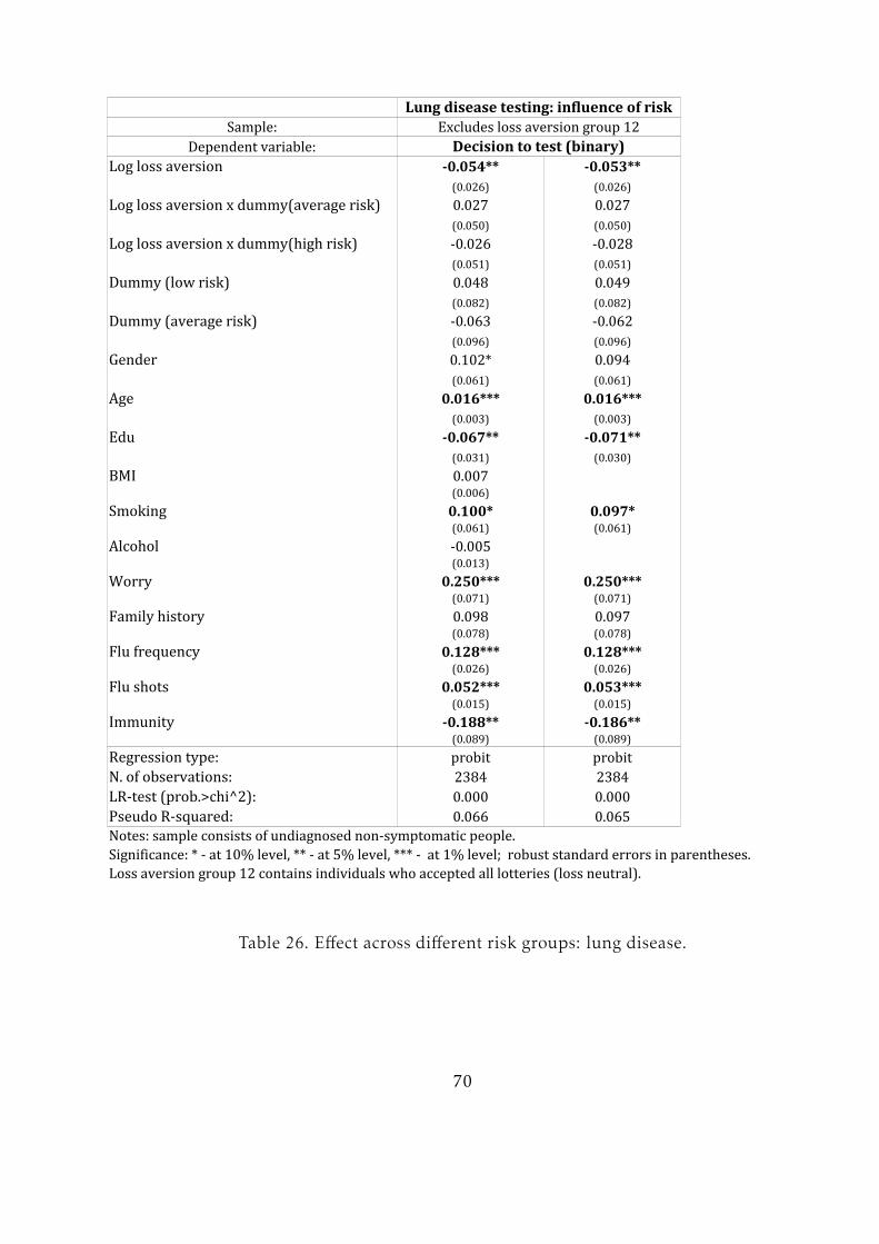
Lung disease testing: influence of riskSample: Excludes loss aversion group 12Dependent variable: Decision to test (binary)Log loss aversion -0.054** -0.053**(0.026) (0.026)Log loss aversion x dummy(average risk) 0.027 0.027(0.050) (0.050)Log loss aversion x dummy(high risk) -0.026 -0.028(0.051) (0.051)Dummy (low risk) 0.048 0.049(0.082) (0.082)Dummy (average risk) -0.063 -0.062(0.096) (0.096)Gender 0.102* 0.094(0.061) (0.061)Age 0.016*** 0.016***(0.003) (0.003)-0.067** -0.071**(0.031) (0.030)BMI 0.007(0.006)Smoking 0.100* 0.097*(0.061) (0.061)Alcohol -0.005(0.013)Worry 0.250*** 0.250***(0.071) (0.071)Family history 0.098 0.097(0.078) (0.078)Flu frequency 0.128*** 0.128***(0.026) (0.026)Flu shots 0.052*** 0.053***(0.015) (0.015)Immunity -0.188** -0.186**(0.089) (0.089)Regression type:N. of observations: 2384 23840.000 0.000Pseudo R-squared: 0.066 0.065Notes: sample consists of undiagnosed non-symptomatic people.Significance: * - at 10% level, ** - at 5% level, *** - at 1% level; robust standard errors in parentheses.Loss aversion group 12 contains individuals who accepted all lotteries (loss neutral).

Edu

probit probitLR-test (prob.>chi^2):

Table 26. Effect across different risk groups: lung disease.

70

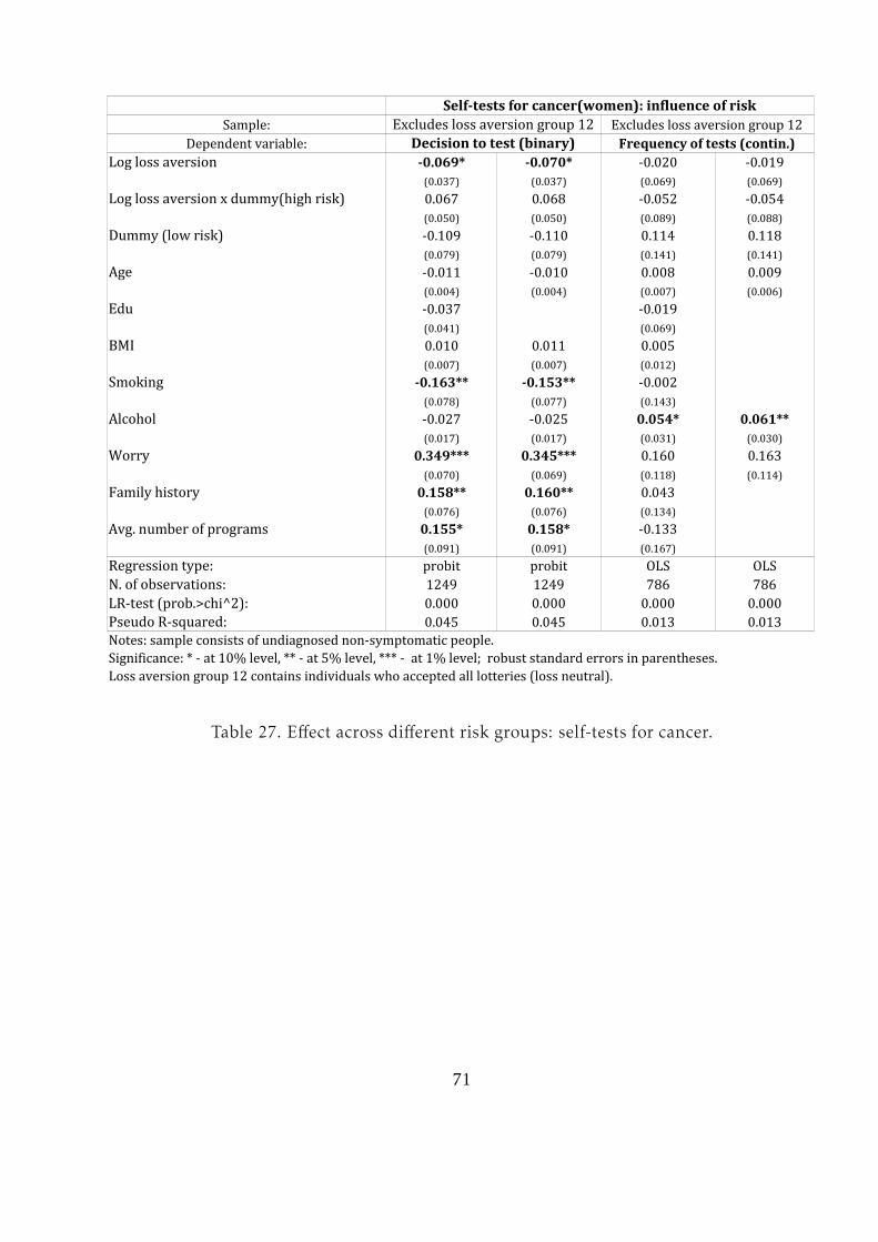
Self-tests for cancer(women): influence of riskSample: Excludes loss aversion group 12 Excludes loss aversion group 12Dependent variable: Decision to test (binary)Log loss aversion -0.069* -0.070* -0.020 -0.019(0.037) (0.037) (0.069) (0.069)Log loss aversion x dummy(high risk) 0.067 0.068 -0.052 -0.054(0.050) (0.050) (0.089) (0.088)Dummy (low risk) -0.109 -0.110 0.114 0.118(0.079) (0.079) (0.141) (0.141)Age -0.011 -0.010 0.008 0.009(0.004) (0.004) (0.007) (0.006)-0.037 -0.019(0.041) (0.069)BMI 0.010 0.011 0.005(0.007) (0.007) (0.012)Smoking -0.163** -0.153** -0.002(0.078) (0.077) (0.143)Alcohol -0.027 -0.025 0.054* 0.061**(0.017) (0.017) (0.031) (0.030)Worry 0.349*** 0.345*** 0.160 0.163(0.070) (0.069) (0.118) (0.114)Family history 0.158** 0.160** 0.043(0.076) (0.076) (0.134)0.155* 0.158* -0.133(0.091) (0.091) (0.167)Regression type: OLS OLSN. of observations: 1249 1249 786 7860.000 0.000 0.000 0.000Pseudo R-squared: 0.045 0.045 0.013 0.013Notes: sample consists of undiagnosed non-symptomatic people.Significance: * - at 10% level, ** - at 5% level, *** - at 1% level; robust standard errors in parentheses.Loss aversion group 12 contains individuals who accepted all lotteries (loss neutral).

Frequency of tests (contin.)

Edu

Avg. number of programs probit probitLR-test (prob.>chi^2):

Table 27. Effect across different risk groups: self-tests for cancer.

71

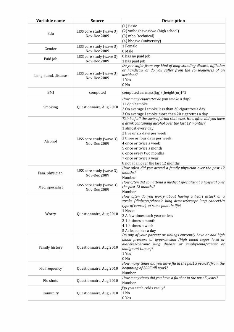
Variable name Source Description(1) BasicGender 1 Female0 MalePaid job 0 has no paid job1 has paid job

Long-stand. disease 1 Yes0 NoBMI computedSmoking Questionnaire, Aug 2010 How many cigarettes do you smoke a day? 1 I don't smoke2 On average I smoke less than 20 cigarettes a day 3 On average I smoke more than 20 cigarettes a day

Alcohol1 almost every day 2 five or six days per week 3 three or four days per week 4 once or twice a week 5 once or twice a month 6 once every two months 7 once or twice a year 8 not at all over the last 12 months NumberNumber

Worry Questionnaire, Aug 2010 1 Never 2 A few times each year or less 3 1-4 times a month 4 1-4 times a week 5 At least once a day Family history Questionnaire, Aug 2010 1 Yes0 NoFlu frequency Questionnaire, Aug 2010 NumberFlu shots Questionnaire, Aug 2010 How many times did you have a flu shot in the past 5 years? NumberImmunity Questionnaire, Aug 2010 Do you catch colds easily? 1 No0 Yes

Edu LISS core study (wave 3), Nov-Dec 2009 (2) vmbo/havo/vwo (high school)(3) mbo (technical)(4) hbo/vo (university)LISS core study (wave 3), Nov-Dec 2009LISS core study (wave 3), Nov-Dec 2009LISS core study (wave 3), Nov-Dec 2009

Do you suffer from any kind of long-standing disease, affliction or handicap, or do you suffer from the consequences of an accident?

computed as: mass(kg)/(height(m))^2

LISS core study (wave 3), Nov-Dec 2009Think of all the sorts of drink that exist. How often did you have a drink containing alcohol over the last 12 months?

Fam. physician LISS core study (wave 3), Nov-Dec 2009 How often did you attend a family physician over the past 12 months?

Med. specialist LISS core study (wave 3), Nov-Dec 2009 How often did you attend a medical specialist at a hospital over the past 12 months?

How often do you worry about having a heart attack or a stroke (diabetes/chronic lung disease(except lung cancer)/a type of cancer) at some point in life?

Do any of your parents or siblings currently have or had high blood pressure or hypertension (high blood sugar level or diabetes/chronic lung disease or emphysema/cancer or malignant tumor)?

How many times did you have flu in the past 5 years? (from the beginning of 2005 till now)?

72

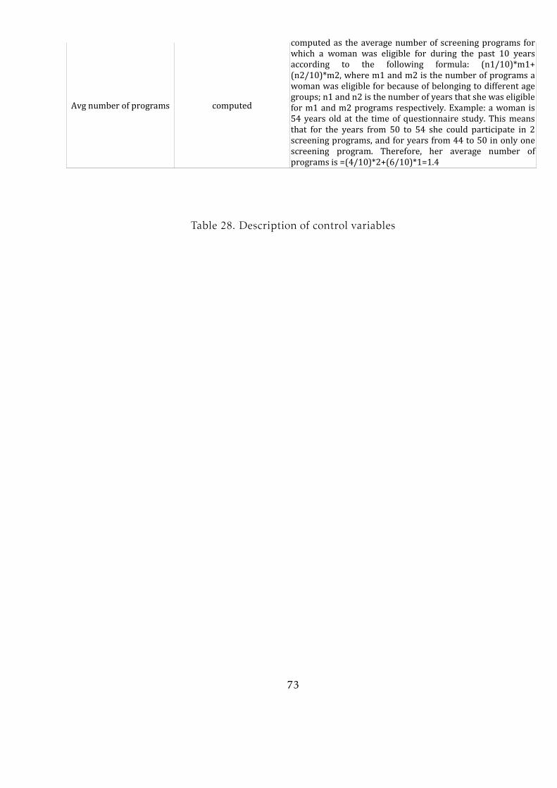
computedAvg number of programscomputed as the average number of screening programs for which a woman was eligible for during the past 10 years according to the following formula: (n1/10)*m1+(n2/10)*m2, where m1 and m2 is the number of programs a woman was eligible for because of belonging to different age groups; n1 and n2 is the number of years that she was eligible for m1 and m2 programs respectively. Example: a woman is 54 years old at the time of questionnaire study. This means that for the years from 50 to 54 she could participate in 2 screening programs, and for years from 44 to 50 in only one screening program. Therefore, her average number of programs is =(4/10)*2+(6/10)*1=1.4

Table 28. Description of control variables

73

References

Abellan-Perpiñan J.M., Bleichrodt H. and Pinto-Prades J.L. (2009), The Predictive Va-

lidity of Prospect Theory Versus Expected Utility in Health Utility Measurement. Jour-

nal of Health Economics, 28, 1039-1047.

Andersen M.R., Smith R., Meischke H., Bowen D. and Urban N. (2003) Breast Can-

cer Worry and Mammography Use by Women with and without a Family History in a

Population-based Sample. Cancer Epidemiol Biomarkers Prev, 12, 314-320.

Basnet R., Hinderaker S.G., Enarson D., Malla P., Morkver O. (2009) Delay in the diag-

nosis of tuberculosis in Nepal. BMC Public Health, 9, 236.

Bleichrodt H. and Pinto J.L. (2002) Loss Aversion and Scale Compatibility in Two-

Attribute Trade-Offs. Journal of Mathematical Psychology, 46, 315-337.

Bowen D., McTiernan A., Burke W., Powers D., Pruski J., Durfy S., Gralow J., Malone

K.(1999) Participation in Breast Cancer Risk Counseling Among Women With a Fam-

ily History. Cancer, Epidemology, Biomarkers, and Prevention, 8, 581-585.

Booij A. and van de Kuilen G. (2009) A Parameter-Free Analysis of the Uitlity for

Money for the General Population under Prospect Theory. Journal of Economic Psy-

chology, vol. 30, pp. 651-666.

Brooks P. and Zank H. (2004) Attitudes on Gain and Loss Lotteries: A Simple Experi-

ment. The School of Economic Studies Discussion Paper Series.

Calder L., WanZhen G. and Simmons G. (2000) Tuberculosis: Reasons for Diagnostic

74

Delay in Auckland. New Zealand Medical Journal, 113:483-485.

Caplan L.S.(1995) Patient Delay in Seeking Help for Potential Breast Cancer. Public

Health Reviews, 23(3), 263-274.

Caplin A. and Leahy J. (2001) Psychological Expected Utility and Anticipatory Feel-

ings. Quarterly Journal of Economics ,116(1), 55-80.

Carman K.G. and Kooreman P. (2011) Flu Shots, Mammograms and the Perception of

Probabilities. working paper

Chen K. and Fabian L. (2008) Education, Information and Improved Health: Evidence

from Breast Cancer Screening. IZA Discussion Paper No. 3548

Fischhoff B. and Manski C. F. (ed. by) Elicitation of Preferences. Published by Kluwer

Academic Publishers, 2000.

Hancock G.R. and Mueller R. (ed. by) The Reviewer’s Guide to Quantitative Methods

in the Social Sciences. Published by: Taylor and Francis e-Library, 2010.

Gonzalez R. and Wu G. (1999) On the Shape of the Probability Weighting Function.

Cognitive Psychology, 38, 129–166.

Harinck F., van Dijk E., van Beest I. and Mersmann P. (2007) When Gains Loom Larger

Than Losses. Reversed Loss Aversion for Small Amounts of Money. Psychological Sci-

ence, vol. 18, no.12.

75

Hjorth K. and Fosgerau M. (2011) Loss Aversion and Individual Characteristics. Envi-

ronmental Resource Economics, 49, 573-596.

Kahneman D. and Tversky A.(1979) Prospect Theory: An Analysis of Decisions under

Risk. Econometrica, Vol.47, No.2, 263-292.

Kash K.M., Holland J.C., Halper M.S. and Miller D.G. (1992) Psychological Distress

and Surveillance Behaviors of Women with a Family History of Breast Cancer. Journal

of the National Cancer Institute, 84(1), 24-30.

Knetsch J.L. (1989) The endowment effect and evidence of nonreversible indifference

curves. American Economic Review, 79, 1277–1284.

Koop G.J. and Johnson J. (2010) The use of multiple reference points in risky decision

making. Journal of Behavioral Decision Making (in press).

Köbberling V. and Wakker P. (2005) An Index of Loss Aversion. Journal of Economic

Theory, Vol. 122, 119-131.

Kőszegi B. (2003) Health Anxiety and Patient Behavior. Journal of Health Economics,

22(6), 1073-1084.

Kőszegi B. and Rabin M. (2006) A Model of Reference-Dependent Preferences. Quar-

terly Journal of Economics, 121(4), 1133-1165.

Kőszegi B. and Rabin M. (2007) Reference-Dependent Risk Attitudes. American Eco-

nomic Review, 97(4), 1047-1073.

76

Kőszegi B. and Rabin M. (2009) Reference-Dependent Consumption Plans. American

Economic Review, 99(3), 909-936.

Leung S.F. and Yu S. (1996) On the Choice Between Sample Selection and Two-Part

Models. Journal of Econometrics, 72, 197-229.

Neuman E. and Neuman S. (2008) Reference-dependent preferences and loss aversion:

A discrete choice experiment in the health-care sector. Judgment and Decision Making,

vol. 3, no. 2, 162-173

Osborne J.W. andOverbay A. (2004) The power of outliers (andwhy researchers should

always check for them). Practical Assessment, Research and Evaluation, 9(6).

Ritov I. and Baron J. (1993) Framing effects in evaluation of multiple risk reduction.

Journal of Risk and Uncertainty, Vol.6, No.2, 145-159.

Rothman A.J., Bartels R., Wlaschin J. and Salovey P. (2006) The Strategic Use of Gain-

and Loss-Framed Messages to Promote Healthy Behavior: How Theory Can Inform

Practice. Journal of Communication, 56, 202-220.

Schweitzer M. (1994) Disentangling status quo and omission effects: An experimental

analysis. Organizational Behavior and Human Decision Processes, 58, 457–476.

Stalmeier P. and Bezembinder T. (1999) The Discrepancy between Risky and Riskless

Utilities: A Matter of Framing? Medical Decision Making, 19, 435.

77

Tversky A. and Kahneman D. (1992) Advances in Prospect Theory: Cumulative Rep-

resentation of Uncertainty. Journal of Risk and Uncertainty, 5(4), 297–323.

Van Osch S., van den Hout W. and Stiggelbout A.M. (2006) Exploring the Reference

Point in Prospect Theory: Gambles for Length of Life. Medical Decision Making, 26,

338-346.

Vernon S. (1999) Risk Perception and Risk Communication for Cancer Screening Be-

haviors: a review. Journal of the National Cancer Institute. Monographs, 25, 101-119.

Wainer H. (1976) Robust statistics: A survey and some prescriptions. Journal of Educa-

tional Statistics, 1(4), 285-312.

Wakker P. P. (2010) Prospect theory: for risk and ambiguity. Published by: Cambridge

University Press.

Wakker P. P. and Deneffe D. (1996). Eliciting von Neumann–Morgenstern utilities

when probabilities are distorted or unknown. Management Science, vol. 42, 1131–1150.

Wu G. and Gonzalez R.(1996) Curvature of the probability weighting function. Man-

agement Science, 42, 1676–1690.

78