OSCILLATION PHYSICS WITH A NEUTRINO FACTORY

M. Apollonio1 , A. Blondel2, A. Broncano3 ,M. Bonesini4 , J. Bouchez5, A. Bueno6, J. Burguet-Castell7 ,M. Campanelli2,∗ , D. Casper8, M.G. Catanesi9 , A. Cervera10, S. Cooper11 ,M. Donega2,A. Donini12,A. de Gouvea13, A. de Min14, R. Edgecock15,16 , J. Ellis17, M. Fechner18 , E. Fernandez19 , F. Ferri4,B. Gavela3, G. Giannini1, D. Gibin14, S. Gilardoni2,16 , J. J. Gomez-Cadenas2,7 , P. Gruber16,A. Guglielmi14, P. Hernandez17 , P. Huber20, M. Laveder14 , M. Lindner20 , S. Lola17,†, D. Meloni12,O. Mena3, H. Menghetti21 , M. Mezzetto14 , P. Migliozzi22 , S. Navas-Concha6 , V. Palladino23 ,I.Papadopoulos24 , K.Peach15, E. Radicioni9 , S. Ragazzi4, S. Rigolin17 , A. Romanino25 , J. Rico6,A. Rubbia6, G. Santin1, G. Sartorelli21 , M. Selvi21 , M.Spiro5, T. Tabarelli4, A. Tonazzo4, M. Velasco26 ,G. Volkov27, W. Winter20, P. Zucchelli10,28

1 University of Trieste and INFN Trieste, Italy2 DPNC, University of Geneva, Switzerland

3 Dep. de Fısica Teorica, Univ. Autonoma de Madrid, Madrid, Spain4 University of Milano 2 Bicocca and INFN Milano, Italy

5 DAPNIA, CEA Saclay, France6 ETH Zurich, Switzerland

7 University of Valencia and IFIC Valencia, Spain8 University of California, Irvine, California, USA

9 INFN Bari, Italy10 CERN EP, Geneva, Switzerland

11 Oxford University, Oxford, United Kingdom12 University of Roma I and INFN Roma I, Italy

13 Fermilab, Batavia, Illinois, USA14 University of Padova and INFN Padova, Italy

15 Rutherford Appleton Laboratory, United Kingdom16 CERN PS, Geneva, Switzerland17 CERN TH, Geneva, Switzerland

18 Departement de Physique de l’Ecole Normale Superieure, Paris, France19 Universidad Autonoma de Barcelona, Spain

20 Tech. U. Munchen, Munich, Germany21 University of Bologna and INFN Bologna, Italy

22 INFN Napoli, Italy23 University of Napoli, Italy

24 CERN IT, Geneva, Switzerland25 Scuola Normale Superiore, Pisa, Italy

26 Northwestern University, Evanston, Illinois, USA27 IFVE, Protvino, Russia

28 INFN Ferrara, Italy† now at HR division, CERN, Geneva, Switzerland

∗ Editor: Mario.Campanelli@cern.ch

CERN-TH/2002-208, hep-ph/0210192

1

Abstract

A generation of neutrino experiments have established that neutrinos mix andprobably have mass. The mixing phenomenon points to processes beyondthose of the Standard Model, possibly at the Grand Unification energy scale. Aextensive sequence of of experiments will be required to measure precisely allthe parameters of the neutrino mixing matrix, culminating with the discoveryand study of leptonic CP violation. As a first step, extensions of conventionalpion/kaon decay beams, such as off-axis beams or low-energy super-beams,have been considered. These could yield first observations of νµ → νe tran-sitions at the atmospheric frequency, which have not yet been observed, anda first measurement of θ13. Experiments with much better flux control canbe envisaged if the neutrinos are obtained from the decays of stored particles.One such possibility is the concept of beta beams provided by the decays ofradioactive nuclei, that has been developed within the context of these studies.These would provide a pure (anti-)electron-neutrino beam of a few hundredMeV, and beautiful complementarity with a high-intensity, low-energy con-ventional beam, enabling experimental probes of T violation as well as CPviolation. Ultimately, a definitive and complete set of measurements wouldoffered by a Neutrino Factory based on a muon storage ring. This powerfulmachine offers the largest reach for CP violation, even for very small values ofθ13.

2

Contents

1 INTRODUCTION 6

2 CURRENT STATUS OF NEUTRINO MASSES AND OSCILLATIONS 92.1 Neutrino Masses . . . . . . . . . . . . . . . . . . . . . . . . . . . . . . . . . . . . . . 9

2.1.1 Laboratory limits . . . . . . . . . . . . . . . . . . . . . . . . . . . . . . . . . . 9

2.1.2 Astrophysical and cosmological constraints on neutrino masses . . . . . . . . . 10

2.1.3 General principles for neutrino masses . . . . . . . . . . . . . . . . . . . . . . . 11

2.1.4 Aspects of models for neutrino masses and mixing . . . . . . . . . . . . . . . . 12

2.1.5 Testing models of neutrino masses . . . . . . . . . . . . . . . . . . . . . . . . . 14

2.2 Oscillation Physics . . . . . . . . . . . . . . . . . . . . . . . . . . . . . . . . . . . . . 17

2.2.1 Relativistic approach to the two-family formula . . . . . . . . . . . . . . . . . . 17

2.2.2 Three families in vacuum . . . . . . . . . . . . . . . . . . . . . . . . . . . . . . 17

2.2.3 Oscillations in matter . . . . . . . . . . . . . . . . . . . . . . . . . . . . . . . . 20

2.2.4 Current status of neutrino mixing parameters . . . . . . . . . . . . . . . . . . . 23

2.2.5 Motivations for new physics . . . . . . . . . . . . . . . . . . . . . . . . . . . . 24

2.2.6 Prospects for the near future . . . . . . . . . . . . . . . . . . . . . . . . . . . . 25

3 CONVENTIONAL NEUTRINO BEAMS 273.1 First-Generation Long-Baseline Neutrino Projects . . . . . . . . . . . . . . . . . . . 27

3.1.1 KamLAND . . . . . . . . . . . . . . . . . . . . . . . . . . . . . . . . . . . . . 27

3.1.2 Long-baseline accelerator-based experiments . . . . . . . . . . . . . . . . . . . 28

3.1.3 K2K . . . . . . . . . . . . . . . . . . . . . . . . . . . . . . . . . . . . . . . . . 29

3.1.4 NuMI . . . . . . . . . . . . . . . . . . . . . . . . . . . . . . . . . . . . . . . . 29

3.1.5 CERN-Gran Sasso . . . . . . . . . . . . . . . . . . . . . . . . . . . . . . . . . 30

3.1.6 JHF-Super-Kamiokande . . . . . . . . . . . . . . . . . . . . . . . . . . . . . . 31

3.1.7 Possible scenario . . . . . . . . . . . . . . . . . . . . . . . . . . . . . . . . . . 31

3.2 Second-Generation Long-Baseline Neutrino Beams . . . . . . . . . . . . . . . . . . 31

3.2.1 JHF-Hyper-Kamiokande . . . . . . . . . . . . . . . . . . . . . . . . . . . . . . 33

3.2.2 Possible off-axis experiments in the CNGS beam . . . . . . . . . . . . . . . . . 33

3.2.3 Studies for a high-energy super-beam at FNAL . . . . . . . . . . . . . . . . . . 34

3.2.4 The SPL super-beam . . . . . . . . . . . . . . . . . . . . . . . . . . . . . . . . 36

3.2.5 Detector scenarios . . . . . . . . . . . . . . . . . . . . . . . . . . . . . . . . . 37

3.2.6 Physics pote ntial . . . . . . . . . . . . . . . . . . . . . . . . . . . . . . . . . . 38

3.2.7 Effect of the inclusion of neutrino spectral information . . . . . . . . . . . . . . 40

4 BETA BEAMS 424.1 Introduction . . . . . . . . . . . . . . . . . . . . . . . . . . . . . . . . . . . . . . . . 42

4.2 Machine Issues . . . . . . . . . . . . . . . . . . . . . . . . . . . . . . . . . . . . . . . 43

4.2.1 Nuclear beta decays . . . . . . . . . . . . . . . . . . . . . . . . . . . . . . . . 43

3

4.2.2 The relativistic effect . . . . . . . . . . . . . . . . . . . . . . . . . . . . . . . . 44

4.2.3 Baseline, energy and intensity considerations . . . . . . . . . . . . . . . . . . . 45

4.3 Physics Reach of the Beta Beam . . . . . . . . . . . . . . . . . . . . . . . . . . . . . 46

4.3.1 Signal . . . . . . . . . . . . . . . . . . . . . . . . . . . . . . . . . . . . . . . . 46

4.3.2 Backgrounds . . . . . . . . . . . . . . . . . . . . . . . . . . . . . . . . . . . . 47

4.3.3 Systematic errors . . . . . . . . . . . . . . . . . . . . . . . . . . . . . . . . . . 48

4.3.4 Beam optimization . . . . . . . . . . . . . . . . . . . . . . . . . . . . . . . . . 48

4.3.5 Sensitivity to CP violation . . . . . . . . . . . . . . . . . . . . . . . . . . . . . 49

4.3.6 Synergy between the SPL super-beam and the beta beam . . . . . . . . . . . . . 51

5 THE NEUTRINO FACTORY 525.1 Overview . . . . . . . . . . . . . . . . . . . . . . . . . . . . . . . . . . . . . . . . . . 52

5.1.1 General principles . . . . . . . . . . . . . . . . . . . . . . . . . . . . . . . . . 52

5.1.2 Rates and backgrounds . . . . . . . . . . . . . . . . . . . . . . . . . . . . . . . 53

5.2 Flux Control and Resulting Constraints on the Decay Ring Design . . . . . . . . . . 56

5.2.1 Absolute flux monitoring . . . . . . . . . . . . . . . . . . . . . . . . . . . . . . 57

5.2.2 Theoretical knowledge of the neutrino fluxes from muon decay . . . . . . . . . . 58

5.2.3 Muon polarisation . . . . . . . . . . . . . . . . . . . . . . . . . . . . . . . . . 58

5.2.4 Neutrino fluxes and muon polarisation . . . . . . . . . . . . . . . . . . . . . . . 62

5.2.5 Effect of beam divergence . . . . . . . . . . . . . . . . . . . . . . . . . . . . . 63

5.2.6 Summary of uncertainties in the neutrino flux . . . . . . . . . . . . . . . . . . . 66

5.3 Detector issues . . . . . . . . . . . . . . . . . . . . . . . . . . . . . . . . . . . . . . . 68

5.3.1 Magnetic calorimetric iron detectors . . . . . . . . . . . . . . . . . . . . . . . . 68

5.3.2 Summary of the properties of active elements in massive iron calorimetric detectors 68

5.3.3 The Monolith design . . . . . . . . . . . . . . . . . . . . . . . . . . . . . . . . 68

5.3.4 The Large Magnetic Detector (LMD) . . . . . . . . . . . . . . . . . . . . . . . 69

5.3.5 A Liquid Argon detector . . . . . . . . . . . . . . . . . . . . . . . . . . . . . . 71

5.3.6 Magnetized liquid argon detectors . . . . . . . . . . . . . . . . . . . . . . . . . 72

5.3.7 A hybrid emulsion detector . . . . . . . . . . . . . . . . . . . . . . . . . . . . . 73

5.4 Oscillation Physics at the Neutrino Factory . . . . . . . . . . . . . . . . . . . . . . . 74

5.4.1 Precision measurements of oscillations . . . . . . . . . . . . . . . . . . . . . . 76

5.4.2 Sensitivity to θ13 . . . . . . . . . . . . . . . . . . . . . . . . . . . . . . . . . . 76

5.4.3 Matter effects . . . . . . . . . . . . . . . . . . . . . . . . . . . . . . . . . . . . 78

5.4.4 CP violation . . . . . . . . . . . . . . . . . . . . . . . . . . . . . . . . . . . . 79

5.4.5 Correlations and choice of baseline . . . . . . . . . . . . . . . . . . . . . . . . 83

5.4.6 Degeneracies . . . . . . . . . . . . . . . . . . . . . . . . . . . . . . . . . . . . 87

5.4.7 T violation . . . . . . . . . . . . . . . . . . . . . . . . . . . . . . . . . . . . . 90

5.4.8 Search for νe → ντ . . . . . . . . . . . . . . . . . . . . . . . . . . . . . . . . . 92

5.5 Search for New Physics at the Neutrino Factory . . . . . . . . . . . . . . . . . . . . . . 92

5.5.1 New physics in short-baseline experiments . . . . . . . . . . . . . . . . . . . . 93

5.5.2 New physics in long-baseline experiments . . . . . . . . . . . . . . . . . . . . . 94

4

6 SUMMARY AND OUTLOOK 96

5

1 INTRODUCTION

Neutrino experiments over 30 years [1], culminating with the Super-Kamiokande atmospheric neutrinodata [2], have provided, for the first time, unambiguous evidence for the existence of physics beyond theStandard Model. This comes from the fact that the νµ to νe flux ratio is far from theoretical expectations,in combination with the nontrivial angular dependence of the atmospheric νµ flux. This ‘atmosphericneutrino puzzle’ cannot be explained by standard means, such as changing the cosmic ray spectrum, orimproving the atmospheric neutrino flux computations. Furthermore, the Super-Kamiokande result is ingood agreement with other, less precise, measurements of the atmospheric neutrino flux [3].

On a different front, solar neutrino experiments [4, 5] have consistently been measuring solar νe

fluxes which are significantly smaller than those predicted by theory [6]. It is equally hard to explainthis ‘solar neutrino puzzle’ by traditional means (dramatically modifying the currently accepted solarmodels, questioning the estimation of systematic effects by some of the experiments, etc.). The recentmeasurement of the solar neutrino flux via neutrino – deuteron scattering performed by the SNO Col-laboration in both charged-current and neutral-current processes provides unambiguous evidence (at thefive-sigma level) that there are active neutrinos other than νe coming from the Sun [5, 7].

Neutrino oscillations provide the simplest and most elegant solution to both the atmospheric andsolar neutrino puzzles. Neutrino oscillations take place if neutrinos have non-degenerate masses and,similar to what happens in the quark sector, the neutrino mass eigenstates differ from the neutrino weak,or flavour, eigenstates. Although less standard solutions to the atmospheric and the solar neutrino puz-zles, such as exotic neutrino decays, or flavour-violating interactions [8] may still be advocated, nosatisfactory single solution to both anomalies other than neutrino oscillations is known.

The implications of the neutrino data are extremely interesting, since they point towards non-zero neutrino masses, which are prima facie evidence for physics beyond the Standard Model. In theabsence of right-handed neutrinos, νR, no Dirac neutrino mass can be generated, while the transformationproperties of the left-handed neutrinos, νL, under SU(2) × U(1) also forbid a renormalisable Majoranamass term. On the other hand, non-zero neutrino masses arise naturally in many extensions of theStandard Model, which generically contain an extended lepton and/or Higgs sector, and possibly newlepton number-violating interactions.

A large number of analyses of the solar, atmospheric and reactor neutrino data can be found in theliterature [9], including two-flavour and three-flavour analyses of the solar data [10], two-flavour analysesof the atmospheric data [11], three-flavour analyses of the combined atmospheric and reactor data [12]and combined analyses of all neutrino data [13]. It turns out that both the solar and the atmosphericneutrino deficits can be accommodated in minimal schemes with three light neutrinos, which may haveeither of the following hierarchical patterns of masses:

(a) The normal hierarchy, in which the masses are fixed by the mass differences required for theatmospheric and solar deficits. The atmospheric neutrino data require m3 ≈ 10−1 to 10−1.5 eV, whilem2 is determined by the solar neutrino squared-mass difference.

(b) Inverted hierarchy solutions, in which |m1| ∼ |m2| |m3|, where m21,2 ∼ ∆m2

atm and∆m12 = ∆m2

sun.

Since oscillation experiments are only sensitive to mass differences of two neutrino species andnot to the absolute values of the masses, normal and inverted solutions with near-degenerate masses arealso allowed.

Information about the absolute neutrino mass scale can be derived from direct searches, and ex-periments looking for neutrinoless double-beta decay if neutrinos are Majorana particles, are sensitive toneutrino masses O(eV) or below. If the masses are close to the upper boundary of this limit, neutrinosmay still provide a significant component of hot dark matter; next generation experiments looking fordirect neutrino mass will probe this scenario, which is however disfavoured by the most recent cosmo-logical observations.

6

Neutrino oscillations (and other types of new physics in the neutrino sector) can potentially beobserved in terrestrial neutrino experiments, by studying, for example, the flux of νe coming from nu-clear reactors [14] or studying the νµ flux from pion or muon decays [15]. The K2K experiment hasreported first results that are consistent with the atmospheric neutrino data [16]. So far, no other ter-restrial evidence for oscillations has been confirmed, although the current results significantly constrainthe neutrino oscillation parameter space. However, the LSND Collaboration has reported an anomalousflux of νe from µ+ decays, which may be interpreted as evidence for νµ ↔ νe oscillations [17]. Thisexperimental evidence has not yet been independently confirmed, but will be put to the test in the nearfuture [18].

The minimal schemes with only three neutrino masses allow only two independent mass differ-ences, and thus the oscillation interpretation of the LSND result cannot be considered, unless a lightsterile neutrino is introduced [19]. In this case, one has to take into account the constraints from cos-mological Big Bang Nucleosynthesis: a sterile neutrino that mixes with an active one, thus being inequilibrium at the time of nucleosynthesis, can change the abundance of primordially produced ele-ments, such as 4He and deuterium. The larger the mixing and the mass differences between the sterileand active neutrinos, the bigger the deviations from the observed light element abundances. This impliesthat models where the sterile component contributes to solar rather than atmospheric neutrino oscillationsare accommodated more easily within the standard nucleosynthesis scenarios. However, recent data onsolar neutrino oscillations disfavor the sterile solution also in this case. In our discussion, we focus onthe minimal schemes with only three light neutrinos. The physics programme of the Neutrino Factorywould be even richer if there were more light neutrinos.

We can hope that future neutrino data will provide important information on the possible mod-els. Indeed, the main goals of the next generation of neutrino experiments include the determination ofneutrino mass-squared differences and leptonic mixing angles. If neutrino oscillations are indeed thesolution to the neutrino puzzles, the measurement of these fundamental parameters is of utmost impor-tance. Moreover, in general we may expect that P (να → νβ) 6= P (να → νβ) and that we may look forCP violation in a neutrino factory [20] by measuring observables of the type

ACP ≡ P (νe → νµ) − P (νe → νµ)

P (νe → νµ) + P (νe → νµ). (1)

In the near future, it is essential to:

• Confirm the atmospheric neutrino puzzle in a terrestrial experiment and determine the ‘atmo-spheric’ mixing parameters. This is one of the driving forces behind the accelerator-based long-baselineneutrino experiments, namely the K2K experiment [16], which started taking data in 1999 and alreadyhas presented some results, the Fermilab NUMI/MINOS [21] project, which is under construction and issupposed to start data-taking in 2005, and the CNGS (CERN neutrinos to Gran Sasso) project [23], whichshould start running in 2006. The CNGS effort also aims to determine whether νµ ↔ ντ is the dominantoscillation channel responsible for the atmospheric neutrino anomaly, by searching for the appearance ofτ leptons from an initially pure νµ beam.

• Establish that the solar neutrino puzzle is indeed due to neutrino oscillations and determinewhat are the ‘solar’ mixing parameters. This is one of the goals of the SNO experiment [24]. Otherexperiments will also contribute significantly to these goals, such as KamLAND [25], which may provideterrestrial confirmation for the solar neutrino puzzle as long as the solar oscillation parameters lie inthe LMA region, and GNO, which may observe anomalous seasonal variations of the solar neutrinoflux [26]. New experiments, such as Borexino [27], which is already under construction and shouldstart taking data in 2003, and a possible upgrade of the KamLAND [25] experiment, may also observeanomalous seasonal variations [28] or a day-night variation [29] of the 7Be solar neutrino flux. It shouldalso be mentioned that a ‘background-free’ version of Borexino, or an experiment to measure the ppsolar neutrino flux, similar to the HELLAZ [30] proposal, should also be able to detect the presence of

7

neutrinos other than νe coming from the Sun [31].

It is very likely that, after the present and the next rounds of neutrino experiments, both the at-mospheric and solar neutrino puzzles will be unambiguously established as signals for new physics.Moreover, neutrino flavour conversions would also be confirmed. Neutrino oscillations, and thereforeunambiguous evidence for neutrino masses and mixing, will be more difficult to establish explicitly bythe observation of an oscillating pattern. However, the K2K data offer a hint of an oscillation effect intheir energy spectrum, KamLAND [25] has an opportunity when studying reactor neutrinos, and this isalso an objective of the MINOS experiment. For atmospheric neutrinos, a possible option for better ob-servations in the future is to build a new generation of larger atmospheric neutrino detectors with higherperformance. Current detector studies include target materials as different as iron [32], liquid argon [23]and water [33].

We set out in this review a multi-step programme for exploring neutrino oscillations and relatedphysics. This includes:

• An intense hadron source, such as could be provided by the Superconducting Proton Linac (SPL)project at CERN, which could yield a low-energy neutrino super-beam.

• The beta-beam concept, which envisages the production of pure νe and νe beams via the decaysof radioactive nuclei stored in a ring.

• The Neutrino Factory itself, in which pure νe and νµ beams, or pure νµ and νe beams, areproduced via the decays of muons stored in a ring.

As we discuss in this report, this multi-step programme represents a systematic scheme for ex-ploring neutrino physics. There are significant synergies between successive steps in the programme. Italso offers unique prospects for short-baseline neutrino physics and studies of rare decays of slow andstopped muons, that are discussed elsewhere [34, 35]. Moreover, in the longer term, the Neutrino Factoryis an essential stepping-stone towards possible muon colliders, as also discussed elsewhere [36].

8

2 CURRENT STATUS OF NEUTRINO MASSES AND OSCILLATIONS

2.1 Neutrino Masses

2.1.1 Laboratory limits

Direct laboratory limits on neutrino masses are obtained from kinematical studies. The most stringentcurrent upper limit is that on the νe mass, coming from studies of the end-point of the electron energyspectrum in Tritium beta decay [37]

mνe ≤ 2.5 eV

For some time, these experiments tended to prefer a negative mass squared, but this problem has nowdisappeared, as has the previous report of a spectral feature near the end-point. The proposed KATRINexperiment aims to improve the sensitivity to mνe ∼ 0.3 eV [38]. Constraints on the mass of νµ arederived from the decay π+ → µ+ + νµ, which leads to the bound [39]

mνµ ≤ 170 keV

This upper limit could be improved by careful studies using the high fluxes provided at the front endof a neutrino factory. Finally, the mass of ντ is constrained by τ decays into multihadron final states:τ− → 2π−π+ντ and τ− → 3π−2π+π0ντ . The current limit is [40]

mντ ≤ 15.5MeV

and experiments at B factories may be sensitive to mντ < 10 MeV. We note that the distinction betweenneutrino flavour and mass eigenstates is unimportant for the above direct upper limits, as long as themass differences indicated by oscillation experiments are much smaller.

An important constraint on Majorana neutrino masses arises from neutrinoless double-β decay [41],in which an (A,Z) nucleus decays to (A,Z + 2) + 2 e−, without any neutrino emission. This could begenerated by the following quark-level interaction:

d + d → u + u + e− + e−

which violates lepton number by two units (∆L = 2). Such a transition could be generated by an exotic,beyond the Standard Model interaction, and any such interaction would necessarily generate a non-zeroMajorana neutrino mass [42]. Assuming that this dominates the neutrinoless double-β decay matrixelement as illustrated in Fig. 1, it can be used to constrain the combination

< mee >≡ |∑

U∗2ei mi|, (2)

which involves a coherent sum over all the different Majorana neutrino masses mi, weighted by theirmixings with the electron flavour eigenstate, which may include CP-violating phases, as discussed below.This observable is therefore distinct from the quantity observed in Tritium β decay.

The interpretation of neutrinoless double-β decay data depends on calculations of the nuclearmatrix elements entering in this process. The strictest limit that had been reported until recently camefrom a study of the 76Ge isotope by the Heidelberg-Moscow Collaboration [43]:

< mee > ≤ 0.2 eV

Subsequently, the data of this experiment have been reanalysed in [44], where evidence for neutrinolessdouble-β decay at a rate corresponding to a mass

< m >= (0.11 − 0.56) eV,

has been reported, with a preferred value of 0.39 eV. However, this interpretation is not yet generallyaccepted. We note that there are proposals capable of improving the sensitivity of neutrinoless double-βdecay experiments by an order of magnitude.

9

d

d

u

u

e

e

ν

W

W

Fig. 1: Diagrammatic representation of the possible role of a Majorana neutrino mass in generating neutrinoless

double-β decay.

2.1.2 Astrophysical and cosmological constraints on neutrino masses

For a review of cosmological and astrophysical limits on neutrino masses, see [45]. Neutrinos muchlighter than 1 MeV have relic number densities that are essentially independent of their masses, yieldinga relic energy density that is linear in the sum of their masses [46]:

Ωνh2 =

(∑

i mνi

94 eV

)

, (3)

where Ων ≡ ρν/ρc, ρν is the neutrino energy density and ρc the critical density, h parametrises theuncertainty in the Hubble parameter and is probably in the range 0.6 ≤ h ≤ 0.9, and the sum in (3)is over all conventional electroweak doublet neutrinos, which are assumed to be metastable 1. Cosmicmicrowave background data and large-redshift supernovae indicate a total matter density Ωm < 0.5,corresponding to

∑

i mνi<∼ 30 eV. Theories of large-scale structure formation suggest that Ων Ωm,

with the remainder of Ωm dominated by cold dark matter [47], and a recent global analysis of data onthe cosmic microwave background radiation, large-scale structure, big-bang nucleosynthesis and large-redshift supernovae yields

∑

i

mνi≤ 2.5 eV.

The small differences in neutrino masses-squared indicated by the oscillation data discuss later thenimply that each neutrino species must weigh <∼ 0.9 eV.

Cosmological nucleosynthesis additionally imposes constraints on possible oscillations betweenconventional active neutrinos and any additional light sterile neutrinos [48]. If these are sufficientlystrong that the relativistic density of additional neutrinos is comparable to that of the active neutrinos, therate of expansion of the universe is affected during nucleosynthesis, and hence the produced abundanceof 4He in particular. The success of conventional calculations of primordial nucleosynthesis suggeststhat

δm2 sin2 θ < 10−6 eV2

1There are also constraints on the lifetimes of unstable neutrinos obtained by requiring that the energy density of the rela-tivistic decay products be below the critical density, and late decays should also satisfy constraints from the cosmic microwavebackground radiation and light-element abundances.

10

for the mass-squared difference δm2 and mixing angle θ between any active and sterile species.

Additional limits on neutrino masses and mixing are obtained from astrophysical processes, suchas supernova physics [49, 50]. The arrival times of neutrinos from SN 1987a have been used to deriveupper limits of about 20 eV on neutrino masses. Oscillations inside a supernova must be consideredin connection with the r-process, and also for the interpretation of any future neutrino signal from agalactic supernova. As a final point in this short discussion, we note that one of the favoured scenariosfor generating the baryon asymmetry in the universe is leptogenesis [51]. In this scenario, CP violationin the decays of massive singlet neutrinos create a lepton asymmetry, which is subsequently recycledby non-perturbative electroweak interactions into a baryon asymmetry. We discuss later the possibilitythat the parameters of such a leptogenesis scenario may be related to neutrino and/or charged-leptonparameters that may be measurable in experiments.

2.1.3 General principles for neutrino masses

There is no fundamental theoretical reason why neutrinos should not have masses and mix with oneanother. It is generally thought that particles are massless if and only if they are associated with an exactgauge symmetry. Examples include the photon and gluon, which are thought to be massless becauseof U(1) and SU(3) gauge symmetries, respectively. There is no exact gauge symmetry associated withlepton number L, so it is expected that lepton number should be violated at some level. If L is violatedby two units: ∆L = 2, then neutrino masses may arise.

On the other hand, the particle content of the minimal Standard Model, in conjunction with gaugeinvariance and renormalisability, allows neither a Dirac nor a Majorana neutrino mass term. A Diracmass of the form m(νLνR + νRνL) cannot arise in the absence of a singlet νR field, whilst a Majoranaterm mνT

Lσ2νL has weak isospin I = 1, and hence would violate SU(2) gauge invariance. However,it is possible to introduce Majorana neutrino masses into the Standard Model, even without postulatingany new particles, at the price of postulating a higher-order non-renormalizable interaction linking twoleft-handed doublet neutrino fields and two Higgs doublets:

(H.L)(H.L)

M, (4)

where H denotes a Higgs doublet field, L denotes a generic lepton doublet field, and M is some (large)mass parameter that is required for dimensional reasons. An interaction of the form (4) would yieldneutrino masses of order

mν ∼ < 0|H|0 >2

M, (5)

which would be mq,` if M < 0|H|0 >. However, an interaction of the type (4) is not satisfactoryfrom a theoretical point of view, because it is non-renormalizable. Therefore, we need to understand thepresence of such a term in the framework of well-motivated extensions of the Standard Model.

The minimal such possibility is to add three heavy singlet-neutrino fields N ci to the Standard

Model, often called right-handed neutrinos, without necessarily expanding the gauge group. Then thefollowing neutrino Dirac and Majorana mass terms are allowed in the Lagrangian:

L = N ci (MνD

)ijLj +1

2N c

i(MνR)ijN

cj + h.c. (6)

where the indices i, j run over three generations, MνD= Yν < 0|H|0 > is the Dirac mass matrix,

and MνRis the Majorana mass matrix for the right-handed isosinglet neutrino sector. The most general

neutrino mass matrix is then

M =

(

0 MνD

MTνD

MνR

)

. (7)

11

The entries in MνDrequire electroweak symmetry breaking, and so must be <∼ mW , whereas the entries

in MνRmay be arbitrarily large. Assuming that MνR

MνD, the light eigenvalues of M are given by

mlightν '

M2νD

MνR

and therefore are extremely suppressed, as is also obvious from the associated diagram shown in Fig. 2.This is the well-known seesaw mechanism [52], which explains naturally why the neutrinos are so muchlighter than the other known fermions.

VLi

VLj

V Rk VR

m

Φ

H H

Fig. 2: Diagrammatic representation of the seesaw mechanism for generating small neutrino masses.

Neutrino mixing arises from the mismatch between the mass eigenstates and the current eigen-states that couple via the weak interactions to charged leptons of definite flavour. The neutrino mixingmatrix is therefore given by

V = V †ν V`, (8)

where V` diagonalizes the charged-lepton mass matrix, and Vν diagonalizes the light neutrino massmatrix mlight

ν [53]. As a unitary 3 × 3 matrix, V would seem to have 9 parameters a priori, but 3 ofthese can be absorbed by phase transformations of the charged-lepton fields, yielding a net total of 6parameters, of which 3 are light-neutrino mixing angles θij : 1 ≤ i 6= j ≤ 3 and 3 are CP-violatinglight-neutrino mixing phases, including the oscillation phase δ and two Majorana phases φ1,2 that appearin the neutrinoless double-β decay observable. Thus, the total number of neutrino parameters that arein principle observable at low energies is 9: 3 light-neutrino masses mlight

ν , 3 real mixing angles and 3CP-violating phases.

However, the minimal seesaw model contains a total of 18 parameters, even after taking intoaccount the possible field redefinitions. In addition to the 9 parameters mentioned above, there areadditionally 3 heavy Majorana neutrino mass eigenvalues MνR

, 3 more real mixing angles and 3 morephases associated with the heavy-neutrino sector [54]. As illustrated in Fig. 3, 12 of these parametersplay a role in generating the baryon number of the universe via leptogenesis, but these do not include θ ij ,δ and φ1,2. Since the lepton number density involves a unitary sum over the light neutrino and leptonspecies, it is insensitive to the values of these light-neutrino mixing angles and phases. However, asalso shown in Fig. 3, 16 of the 18 neutrino parameters contribute to renormalization effects that are, inprinciple, measurable in a supersymmetric version of the minimal seesaw model.

2.1.4 Aspects of models for neutrino masses and mixing

Our experimental knowledge of the 18 neutrino parameters introduced above is limited so far to 4: 2neutrino mass-squared differences, and 2 mixing angles. As we discuss later in more detail, the dataindicate that these 2 measured neutrino mixing angles are probably both quite large, possibly even max-imal, whilst the third angle is relatively small. Since the seesaw mechanism suggests that the origins ofneutrino masses and mixings are different from, and more complicated than those of quarks, we should,

12

Yν , MNi

15+3 physicalparameters

Seesaw mechanismMν

9 effective parameters

LeptogenesisYνY

†ν , MNi

9+3 parameters

RenormalizationY

†νLYν , MNi

13+3 parameters

Fig. 3: Roadmap for the physical observables derived from Yν and Ni.

in retrospect, perhaps not have been so surprised that some neutrino mixing angles are larger than thosein the quark sector. The spate of experimental information on neutrino masses and mixing, and theirunexpected nature, has spawned many theoretical models, some of whose general features we reviewbelow. The neutrino factory is uniquely well placed to provide crucial input for distinguishing betweensuch models, in particular via neutrino-oscillation experiments. Models for neutrino masses and mix-ing typically incorporate ideas for family (or generation) symmetries and/or grand unification schemeslinking quarks and leptons, and we now give examples of each.

U(1) Flavour Symmetries

The left- and right-handed components of quarks and leptons may be assigned various U(1)charges, as are the Higgs fields, such that only one or a limited number of entries in the mass matrices canbe generated by renormalizable terms in the effective Lagrangian [55]. Additional entries become per-mitted if the symmetry is broken, for example by one or more vacuum expectation values V for fields thatappear in non-renormalizable terms in the mass matrices, scaled by inverse powers of larger masses M .This type of scheme provides a perturbative expansion in powers of some small parameter ε ≡ V/M . Ina popular class of realizations, only the (3,3) element of the associated mass matrix is non-zero at leadingorder, whilst other terms arise with various powers of ε, that are fixed by the U(1) charge assignments:

M ∼

εm εn εp

εq εr εs

εt εu 1

(9)

In such models, each term in the mass matrix has a numerical coefficient that may be calculated onlywith a more complete theory.

13

In its absence, there are numerical ambiguities in the predictions of such a model, but mixingangles are generically powers of ε. There are two possible ways to obtain large mixing angles in sucha perturbative U(1) framework. One of the mixing matrices may contain more than one entry appear-ing with the same power of ε, for example perhaps the (3, 3) and (3, 2) entries in (9) might both beO(1). Alternatively, the numerical coefficients might be such as to compensate for the ‘small’ expansionparameter ε.

Grand Unified Theories

In a generic scheme, there is a lot of freedom in assigning the various U(1) flavour charges.However in Grand Unified Theories, quark and lepton fields that belong in the same GUT multipletshave the same flavour charges. This introduces additional constraints, thus increasing predictivity [56].For instance, in SO(10) models, all quarks and leptons are accommodated in a single 16 representationof the group, implying left-right symmetric mass matrices with similar structures for all fermions. As aconsequence, such GUT models predict Vµτ ≈ Vcb, which is inconsistent with the data. Hence, in orderto construct a viable SO(10) solution, one must consider the effects of the additional Higgs multipletsthat break SO(10) down to SU(3) × SU(2) × U(1). However, this introduces additional parameters,thus decreasing predictivity.

The situation is different in SU(5) unification, where the (q, uc, ec)i fields (for left-handed quarks,right-handed up quarks and right-handed charged leptons, respectively) belong to 10 representations, the(`, dc)i fields (for left-handed leptons and right-handed down quarks, respectively) belong to 5 represen-tations, and the Ni (singlet neutrinos) to singlet representations of the group. In this case, the up-quarkmass matrix is symmetric, there is a lot of freedom in chosing the neutrino mass matrices, and thecharged-lepton mass matrix is the transpose of the down-quark one. Hence the mixing of the left-handedleptons is related to that of the right-handed down quarks, and not with the small CKM mixing of theleft-handed quarks. Thus, SU(5) can in principle accommodate large MNS neutrino mixing at the sametime as small CKM quark mixing, without any tuning of parameters.

In left-right symmetric models, one has identical U(1) flavour charges for the left- and right-handed fields, as in SO(10) unification, but quarks and leptons need not be correlated. This leads tosymmetric quark, lepton and neutrino mass matrices, but allows the lepton mixing to be independent ofthat in the quark sector.

Non-Abelian Flavour Symmetries

Specific U(1) flavour models may yield one relatively large neutrino mixing angle, but tend tofavour small values of the other mixing angles and hierarchical neutrino masses. Thus, such models arecomfortable with the small value of θ13, but could be embarrassed if the current preference for the LMAsolar solution is confirmed. This feature of models with Abelian flavour symmetries may be traced to thelack of charge quantization and arbitrary coefficients, making it difficult to obtain accurate cancellationsbetween the various entries of the mass matrices, unless extra assumptions are made, for example in theheavy singlet-neutrino sector.

The situation is reversed in non-Abelian models. To illustrate this, consider a simple case inwhich the lepton fields are SO(3) triplets. In this case, degenerate lepton textures are to be expected.Subsequently, one may break SO(3) so that there are large mass splittings for charged leptons, but notfor the light neutrinos [57]. This means that, in schemes with non-Abelian flavour symmetries, solutionswith degenerate neutrinos and bimaximal mixing can be generated in a natural way. On the other hand,the understanding of any small mixing angles and phases might then become an issue.

2.1.5 Testing models of neutrino masses

The neutrino oscillation measurements that can be made at a neutrino factory, notably the magnitudesof θ13 and δ, will provide important constraints on models of neutrino masses. For example, as just

14

discussed, the expected size of δ and other CP-violating phases may be rather different in Abelian andnon-Abelian flavour models.

When comparing model predictions with data, care must be taken to include the effects of quantumcorrections in the neutrino parameters, which cause them to vary as functions of energy [58]. To leadingorder, entries in the neutrino mass matrix are renormalized by multiplicative factors [59]:

mlightν (Q)

ij= mlight

ν (MN )ij × Ii × Ij , (10)

where the mlightν (MN )

ij, i = e, µ, τ denote the initial mass entries at the high-energy energy scale where

the neutrino mass matrix is generated, and the

Ii ≡ exp[1

16π2

∫ t

t0

Y 2i dt] : t ≡ lnµ (11)

are integrals determined by the running of the charged-lepton Yukawa couplings Yi as functions of therenormalisation scale µ. This effect implies that the neutrino mixing can be amplified or even destroyed,as we go from high to low energies, and the neutrino mass eigenvalues may also be altered significantly.Although these renormalization effects are not significant for schemes with hierarchical neutrino masses,they are potentially large in models with degenerate neutrinos and may be important in models withbimaximal mixing. For instance, for the neutrino mass texture

mlightnu ∝

0 1√2

1√2

1√2

12 −1

21√2

−12

12

which would seem to lead to bimaximal mixing, Fig. 4 indicates a large change of the eigenvalues whenrunning from high to low energies [59], and analogous large effects may also occur in the mixing angles.

In supersymmetric seesaw models, quantum corrections may provide other ways of measuringneutrino parameters and testing models via lepton-flavour-violating processes. In the minimal seesawmodel without supersymmetry, the amplitudes for processes such as µ → eγ, µ-e conversion in nuclei,µ → eee and τ → `γ, 3` [60, 34, 61] where ` = e, µ denotes a generic light charged lepton, areproportional to the neutrino mass-squared difference, and so are many orders of magnitude smaller thanthe existing experimental bounds. This is no longer the case in supersymmetric theories, due to theexistence of loop diagrams with internal sparticles, that may violate charged-lepton numbers. This mayhappen either because sfermion masses are not diagonal in the lepton flavour basis already at the inputscale MGUT , in which case very large lepton-flavour violating rates are generically predicted [60], orbecause flavour-violating effects are induced by quantum corrections [62].

These are generic in the Minimal Supersymmetric Standard Model with heavy singlet neutrinos,because the Dirac Yukawa couplings to neutrinos and charged leptons cannot, in general, be diagonalizedsimultaneously. Since both these sets of lepton Yukawa couplings appear in the renormalization-groupequations, the slepton mass matrices receive off-diagonal contributions. In the leading-logarithmic ap-proximation, in the basis where the charged-lepton Yukawa couplings are diagonal, these are given by

(

δm2˜

)i

j∝ 1

16π2(3 + a2)

(

Y †ν

)i

kLk (Yν)

kj m2

0, (12)

where Lk ≡ ln MGUT

MNk

, the singlet-neutrino mass MNkis the scale above which the Dirac Yukawa cou-

pling Yν appears in the renormalization-group equations, a is related to the trilinear mass parameter, andm0 is the common value of the scalar masses at the GUT scale.

In this class of models, the rates predicted for processes violating charged-lepton flavour may beclose to the current experimental bounds, and are in principle sensitive to up to 16 of the 18 parameters in

15

-2 -1.5 -1 -0.5 0 0.5Log10HYΤ0 L

-5

-4

-3

-2

-1

ÈÈm iÈ-

Èm jÈÈ

Fig. 4: Renormalization of meff eigenvalues in a model which would seem to lead to bimaximal mixing. The

range of initial values of the τ Yukawa coupling chosen correspond to values of tanβ in the range 1 to 58, assuming

MN = 1013 GeV.

the minimal seesaw model, as indicated in Fig. 3 [54]. Therefore, different models predict in general dif-ferent rates for the different charged-lepton flavour-violating processes: the larger the lepton mixing andthe larger the neutrino mass scales, the larger the rates. Consequently, schemes with degenerate eV neu-trinos and bimaximal mixing generally yield significantly larger effects than schemes with hierarchicalneutrinos and small mixing angles.

The prospects for measuring some of these processes at the front end of a neutrino factory arediscussed elsewhere [34]. Here we just note that the present experimental upper limits on the mostinteresting of these processes are BR(µ → eγ) < 1.2 × 10−11 [63] and R(µ−T i → e−T i) < 6.1 ×10−13 [64], and that projects are underway to improve these upper limits significantly. An experimentwith a sensitivity BR(µ → eγ) ∼ 10−14 is being prepared at PSI [65] and the MECO experiment with asensitivity to R(µ−N → e−N) ∼ 10−17 has been proposed for BNL [66], whilst the PRISM project [67]and a neutrino factory [34] may reach sensitivities to BR(µ → eγ) ∼ 10−15 and Br(µ → eee) ∼ 10−16.The latter sensitivity may open the way to measuring the T-odd, CP-violating asymmetry AT (µ → eee).Other measurements that may be sensitive to CP violation in the lepton sector include those of the electricdipole moments of the electron and muon, and a neutrino factory would also have unique sensitivity tothe latter [34].

In this way, the front end of the neutrino factory could contribute to determining as many as 16of the 18 parameters in the neutrino sector, via their renormalization of soft supersymmetry-breakingparameters (see Fig. 3). Any such information would therefore provide useful constraints on neutrinomodels. Moreover, the combination of such front-end data with oscillation data from the neutrino factorymay enable the baryon number of the universe to be calculated, if it is due to leptogenesis in the minimalsupersymmetric version of the seesaw model.

16

2.2 Oscillation PhysicsNeutrino oscillations in vacuum would arise if neutrinos were massive and mixed [68] similar to whathappen in the quark sector. If neutrinos have masses, the weak eigenstates, να (α = e, µ, τ, ...), producedin a weak interaction are, in general, linear combinations of the mass eigenstates νi (i = 1, 2, 3, ...). Wenow review the basic physics of neutrino oscillations in vacuum and in matter.

2.2.1 Relativistic approach to the two-family formula

In the simpler case of two-family mixing, one has:(

να

νβ

)

=

(

cos θ sin θ− sin θ cos θ

)(

ν1

ν2

)

(13)

We use the standard approximation that |ν〉 is a plane wave and consider its propagation in a one-dimensional space. A mass eigenstate produced at t,x=0, will evolve in space and in time as:

|νi(t, x)〉 = ei(pix−Eit)|νi〉 for i = (1, 2). (14)

Starting from a flavour eigenstate |να〉, the probability for detecting a state 〈νβ| at a distance L and timet is given by:

P (να → νβ) ≡ |〈νβ|να(t, L)〉|2 = sin2 2θ sin2

[

(p1 − p2)L − (E1 − E2)t

2

]

. (15)

In the ‘same-energy prescription’, which is consistent with the wave-packet treatment 2, one assumesthat the two neutrino mass eigentstates have the same energy, E1 = E2 = E, but different momentum:

p1 =√

E2 − m21 , p2 =

√

E2 − m21 + ∆m2

12 (with ∆m212 ≡ m2

1 − m22) (16)

which leads to:

P (να → νβ) = sin2 2θ sin2 (p1 − p2)L

2' sin2 2θ sin2

(

κ∆m2

12L

E

)

, (17)

In (17) κ is 1/4 in natural units (h = c = 1) or 1.27 if we consider practical units where the energy isexpressed in GeV, the distance in km and the mass difference squared in eV2.

2.2.2 Three families in vacuum

In the three-family scenario, the general relation between the flavour eigenstates να and the mass eigen-states νi is given by the 3x3 mixing matrix V :

V = UA, (18)

where the matrix A contains the Majorana phases

A =

eiα 0 00 eiβ 00 0 1

(19)

2For a detailed discussion, see for example [69] and [70].

17

µ

νe

ν

θ12 θ13

’θ23

ν

ν2

ν1

ν3

ντ

Fig. 5: Representaion of the 3-dimensional rotation between the flavor and mass neutrino eigenstates.

that are not observable in oscillation experiments, and U is the MNSP matrix [68, 71], which is usuallyparameterized by [72] 3:

U =

Ue1 Ue2 Ue3

Uµ1 Uµ2 Uµ3

Uτ1 Uτ2 Uτ3

=

c12c13 s12c13 s13e−iδ

−s12c23 − c12s13s23eiδ c12c23 − s12s13s23e

iδ c13s23

s12s23 − c12s13c23eiδ −c12s23 − s12s13c23e

iδ c13c23

(20)

where, for the sake of brevity, we write sij ≡ sin θij , cij ≡ cos θij . The relevant angles can be derivedfrom the matrix elements via the following relations:

tan2 θ23 ≡ |Uµ3|2|Uτ3|2

, (21)

tan2 θ12 ≡ |Ue2|2|Ue1|2

, (22)

sin2 θ13 ≡ |Ue3|2, (23)

sin δ ≡8 Im(U∗

e2Ue3Uµ2U∗µ3)

sin 2θ12 sin 2θ23 sin 2θ13 cos θ13. (24)

The relations between mass and flavor eigenstates can be visualized as rotations in a three-dimensionalspace, with the angles defined as in Fig. 5.

With a derivation analogous to the two-family case, the oscillation probability for neutrinos reads

P (να → νβ) =∑

jk

Jαβjke−i∆m2

jkL/2E (25)

where Jαβjk = UβjU∗βkU

∗αjUαk. For antineutrinos, the probability is obtained with the substitution

Jαβjk → J∗αβjk. As Jαβjk is not real in general, due to the phase δ, neutrino and antineutrino oscillation

probabilities are different, and therefore CP is violated in the neutrino mixing sector. The CP-even and3Notice, though, that our convention for the sign of δ is opposite from that used in this reference. The MNSP matrix is the

leptonic analogue to the CKM [73] matrix of the quark sector.

18

CP-odd contributions in the oscillation probability can easily be distinguished by separating the real andimaginary parts of Jαβjk:

P (να → νβ) = δαβ − 4∑

j>k

Re(Jαβjk) sin2∆m2

jkL

4E+ 2

∑

j>k

Im(Jαβjk) sin∆m2

jkL

2E. (26)

The Jarlskog determinant J [74] is defined by:

Im(Jαβjk) = J∑

γ,l

εαβγ εjkl (27)

and can be expressed in terms of the mixing parameters, as:

J = c13 sin 2θ12 sin 2θ13 sin 2θ23 sin δ. (28)

We define a complex quantity J whose real part is J :

J = c13 sin 2θ12 sin 2θ13 sin 2θ23eiδ . (29)

Oscillations in a three-generation scenario are consequently described by six independent parameters:two mass differences (∆m2

12 and ∆m223), three Euler angles (θ12, θ23 and θ13) and one CP-violating

phase δ. As an example, we give the full oscillation probability for the oscillation νe → νµ:

P (νe → νµ) = P (νµ → νe) =

4c213[sin

2 ∆23s212s

213s

223 + c2

12(sin2 ∆13s

213s

223 + sin2 ∆12s

212(1 − (1 + s2

13)s223))]

− 1

4|J | cos δ[cos 2∆13 − cos 2∆23 − 2 cos 2θ12 sin2 ∆12]

+1

4|J | sin δ[sin 2∆12 − sin 2∆13 + sin 2∆23], (30)

where we have used the contracted notation ∆jk ≡ ∆m2jkL/4E [75]. The second and third lines are the

CP-violating terms, and are proportional to the imaginary and real parts of J , respectively.

The present experimental knowledge on neutrino oscillation parameters indicates ∆m212 ∆m2

23

and small values for θ13. In this situation, a good and simple approximation for the νe → νµ transitionprobability is obtained by expanding to second order in the small parameters, θ13,∆12/∆13 and ∆12

[116]:

Pνeνµ = s223 sin2 2θ13 sin2 ∆23 + c2

23 sin2 2θ12 sin2 ∆12 + |J | cos (δ − ∆23) ∆12 sin∆23 .(31)

We refer to the three terms in (31) as the atmospheric P atmν(ν) , solar P sol, and interference P inter

ν(ν) terms,respectively [117]. It is easy to show that

|P interν(ν) | ≤ P atm

ν(ν) + P sol, (32)

implying two very different regimes. When θ13 is relatively large or ∆m212 small, the probability is dom-

inated by the atmospheric term, since P atmν(ν) P sol. We will refer to this situation as the atmospheric

regime. Conversely, when θ13 is very small or ∆m212 large, the solar term dominates: P sol P atm

ν(ν) . Thisis the solar regime. The interference term is relevant only if either ∆m2

12 or θ13 are non-negligible. Thepossibility of observing CP violation in neutrino oscillations is connected to the possibility of separatingthe interference term from the solar and atmospheric contributions in (31).

19

ν

ν2

ν1

3

neutrino

∆ 23m

squared

∆m12

2

2

atmospheric, 3 10-3

solar < 210-4 ev2

ev 2

masses ν2

ν1

∆m122 solar < 210-4

neutrino

ev2

ν3

m∆ 223 atmospheric, 3 10-3 ev 2

squaredmasses

Fig. 6: Two possible configurations for the neutrino mass texture: direct (left) or inverted (right).

If we neglect completely ∆m212, setting it to zero4, oscillation probabilities take the simplified

form

P (νe → νe) = 1 − sin2 2θ13 sin2 ∆23 (33)

P (νe → νµ) = sin2 2θ13 sin2 θ23 sin2 ∆23 (34)

P (νe → ντ ) = sin2 2θ13 cos2 θ23 sin2 ∆23 (35)

P (νµ → νµ) = 1 − 4 cos2 θ13 sin2 θ23(1 − cos2 θ13 sin2 θ23) sin2 ∆23 (36)

P (νµ → ντ ) = cos4 θ13 sin2 2θ23 sin2 ∆23. (37)

As expected CP-violating effects are absent since they require the interference of oscillations from twomass differences.

2.2.3 Oscillations in matter

So far, we have analyzed neutrino oscillations in vacuum. When neutrinos travel through matter (e.g.in the Sun, Earth, or a supernova), their coherent forward scattering from particles they encounter alongthe way can significantly modify their propagation. As a result, the probability for changing flavor canbe rather different from its vacuum value. This is known as the Mikheyev-Smirnov-Wolfenstein (MSW)effect [82].

The reason is simple: matter contains electrons but no muons or taus. Neutrinos of the three flavorsinteract with the electrons, the protons and the neutrons of the matter via neutral currents (NC). Electronneutrinos in addition interact with electrons via the charged current (CC). Since the W mass is muchlarger than typical center-of-mass energies for neutrino scattering, the relevant parts of the Lagrangianfor electron neutrinos can be written in the Fermi approximation

L = νe(i∂/ − m)νe − 2√

2GF (νeLγµνeL)(eLγµeL). (38)

The latter term modifies the effective mass of the νe when it goes through matter and, consequently, thetransition probability changes. In the electron reference frame only the γ0 part of the electron currentcontributes, being just the number operator:

< eLγ0eL >= ne/2 (39)

with ne the electron density given by:

ne = NA × Ye × ρ(r) , (40)

and Ye = Z/A and ρ are the electron fraction and the density of the medium. Both of them depend onthe physical propierties of the medium traversed by the neutrinos. For the Earth’s mantle, Ye = 0.494,

4This is a good approximation if LOW or VO solutions happen to be the one chosen by nature for the solar oscillation.

20

and for the Earth’s core Ye = 0.466 [76]. The contribution to the νe effective Hamiltonian due to the CCinteraction with matter is consequently given by:

A =√

2GF ne . (41)

For antineutrinos A has to be replaced by −A, so the behaviour in matter of neutrinos and antineutrinos isdifferent (matter is not CP invariant). In the treatment of oscillations, the extra potential only appears forelectron neutrinos, so the oscillatory terms will no longer be proportional to the mass-squared differencesbetween the three families, but to effective masses-squared that result from the diagonalization of theHamiltonian:

U

m21 0 0

0 m22 0

0 0 m23

U † +

D 0 00 0 00 0 0

, (42)

with D = ±2AEν (depending if neutrinos or antineutrinos are considered).

The diagonalization of the 3-family Hamiltonian in the presence of the extra matter term modifiesthe effective mixing angles appearing in oscillation formulae. It has to be noticed that the ordering ofthe masses in the Hamiltonian is relevant, and the effect of matter is swapped between neutrinos andantineutrinos in the cases of direct and reversed mass hierarchy, as seen in Fig. 6. Thus, the effect ofmatter in a neutrino oscillation experiment allows the determination of the sign of ∆m2

23.

The full formulae for the effective quantities (mass differences and angles) in a three-family sce-nario are quite complicated, and can be found in [77] and [78]. However, it can be shown that, in thecase |∆m2

12| |∆m213| ≈ |∆m2

23|, the three-family mixing decouples into two independent two-familymixing scenarios, even in the presence of matter effects [20]. For energies not too small with respectto that of the oscillation maximum (where |∆m2

23L/E| ≈ 1), the effective oscillation parameters willbecome (see Fig. 7 [78]):

sin2 θm23(D) ' sin2 θ23 (43)

sin2 2θm12(D) ' ∆m2

12

Dsin 2θ12 (44)

sin2 2θm13(D) ' sin2 2θ13

F(45)

δm ' δ (46)

∆M212 ' D (47)

∆M223 ' ∆m2

23

√F (48)

(49)

where we have defined

F ≡ sin2 2θ13 + (D

∆m223

− cos 2θ13)2. (50)

As expected, we see explicitly that all the angles return to their original values in the limit of small matterdensity D → 0 (i.e. F → 1) in the limit ∆m12 ∆m13 and ∆m12 D.

At the Mikheyev-Smirnov-Wolfenstein (MSW) resonance energy

Eresν (GeV ) =

cos 2θ13∆m223

2√

2GF ne

' 1.32 × 104 cos 2θ13∆m223(eV

2)

ρ(g/cm3)(51)

21

0

0.2

0.4

0.6

0.8

1

1.2

1.4

0 0.5 1 1.5 2 2.5 3D/∆m2 32D/∆m2 32D/∆m2 32

0

0.2

0.4

0.6

0.8

1

1.2

1.4

0 5 10 15 20 25 30 35

Eν (GeV) for ρ=3.7 g/cm3

Fig. 7: Evolution of the effective angles in matter as a function of D.

the value of sin2 2θm13 becomes equal to 1, independently of the actual value of the angle in vacuum. Also

the effective value of ∆m232 is significantly modified. If we take ∆m2

23 = 2.5 × 10−3 eV2, θ13 1 andρ = 2.8 g/cm3, the energy of this MSW resonance is 11.8 GeV.

To see how this affects the oscillation probability, we can take the simplified formula for theνe → νµ oscillation in vacuum, as appears in (31), and neglect the mass difference ∆12. Replacingthe vacuum parameters with their effective values, one obtains the approximate νe → νµ oscillationprobability in matter:

P (νe → νµ) = sin2 2θm13 sin2 θm

23 sin2 ∆m23 =

sin2 2θ13

Fsin2 θ23 sin2

(

∆m223

√F

L

4E

)

, (52)

and the oscillation probability at the MSW resonance energy becomes

P (νe → νµ;Eres) = sin2 θ23 sin2

(

∆m223 sin 2θ13

L

4Eres

)

. (53)

If we assume that sin 2θ13 is small, and if the distance L is not too far away from that of the firstmaximum, the probability reads:

P (νe → νµ;Eres) ≈ s223 sin2 2θ13 ×

(

∆m223

L

4Eres

)

. (54)

In the limit ∆m223L/4E 1, this coincides with the vacuum expression of (34). This is why it is

not possible to measure the sign of ∆m223 if the baseline is too short. Matter effects become visible

22

at distances where the argument of the sin function approaches π/4. The oscillation maximum for thevalue Eres = 11.8 GeV and ∆m2

23 = 2.5 × 10−3 eV2 is L = 2300 km, so matter effects start to bevisible as an enhancement of the oscillation probability around the MSW resonance energy for baselineslonger than about 1000 km. For antineutrinos the effective mixing angle is smaller than the real one. Forsmall baselines, a similar compensation as in (54) takes place, but at distances where matter effects startto play a role the oscillation probability in matter is smaller than that in vacuum.

The above considerations are valid near the resonance energy, in other words for D ≈ ∆m223. If

D > ∆m223 i.e., Eν > 2Eres, the effective mixing angle is always smaller than the vacuum one, and the

effect of matter is again a suppression of the oscillation probability.

2.2.4 Current status of neutrino mixing parameters

We assume that active neutrino oscillations are indeed the solution to the neutrino puzzles, and that thereare only three light neutrino species. As discussed above, in this case the Standard Model is augmentedby at least 9 new parameters, of which 3 are neutrino masses, 3 are real mixing angles, there is oneoscillation phase and two additional Majorana phases, which exist only if the neutrinos are Majoranaparticles. Neutrino oscillation experiments, however, are not sensitive to the Majorana phases, and weset them to zero henceforth.

The angles θ23 and θ12 are thought to be mainly responsible for solving, respectively, the atmo-spheric and solar neutrino puzzles, as long as |∆m2

23| > |∆m212| (normal neutrino mass hierarchy). If

the opposite happens to be true (|∆m223| < |∆m2

12|, an inverted mass hierarchy), the definitions abovecan still be related to the appropriate neutrino puzzles, as long as the mass eigenstates are relabelled3 → 2 → 1 → 3. We make this assumption henceforth, and refer to θ23 ≡ θatm, θ12 ≡ θsun. Thus,the third mass eigenstate is defined as the one whose mass squared is ‘further away’ from the other two,which are arranged in ascending order of masses-squared, without any loss of generality. Given thischoice, the inverted hierarchy differs from the normal hierarchy by the sign of ∆m2

23. The entire oscilla-tion parameter space is spanned by varying the three mixing angles from 0 to π/2, keeping ∆m2

12 > 0 5,∆m2

23 (including the sign), and varying δ from −π to π.

The current knowledge of the oscillation parameters can be summarized as follows. There isgood evidence that |∆m2

23| ∆m212, and therefore ∆m2

23 ' ∆m213. This being the case, the current

atmospheric data are sensitive to |∆m223|, tan2 θatm, and |Ue3|2, while the current solar data are sensitive

to ∆m212, tan2 θsun, and |Ue3|2. The Chooz and Palo Verde reactor experiments, when considered in

combination with the solar data, constrain |Ue3|2 as a function of |∆m223|. The experimentally allowed

range of the parameters depends on a number of assumptions: which experimental data are considered,how many neutrino species participate in the oscillation, what was the statistical recipe used to defineallowed regions, etc. We comment briefly later on some of these points. In this Section, we simply quotethe current ‘standard’ results, with some appropriate references.

For the atmospheric and reactor parameters, one obtains [13] at the 99% confidence level (CL),

|Ue3|2 < 0.06, (55)

0.4 < tan2 θatm < 2.5, (56)

1.2 × 10−3 eV2 < |∆m223| < 6.3 × 10−3 eV2. (57)

The situation of the solar parameters is less certain, and is best described graphically. Fig. 8 depicts theresult of the most recent analysis of all solar neutrino data [81], which uses the current version of thestandard solar model [6], but allows the 8B neutrino flux to float in the fit. This particular analysis isperformed assuming two-flavour oscillations, a scenario which is realised in the three-flavour case for

5In two-flavour solar data analyses, it is important also to keep the mixing angle from 0 to π/2 if ∆m2 > 0 is fixed, inorder to cover the entire parameter space [29, 80].

23

|Ue3|2 = 0. The changes to the allowed regions are not qualitatively significant for values of |Ue3|2 upto the upper bound quoted above: in fact, the allowed regions grow, even for |Ue3|2 = 0, simply becausethe confidence level contours are defined for three instead of two degrees of freedom. The right panelof Fig. 8 exhibits the impact of the recent neutral-current measurement from SNO on the preferred solarneutrino oscillation parameters.

Fig. 8: Global fits to current so-

lar neutrino data [81], leaving free the8B neutrino flux. The best-fit point is

marked by the star, while the allowed re-

gions are shown at 90%, 95%, 99%, and

99.73% CL. Here, ∆m2 ≡ ∆m212 and

tan2 θ ≡ tan2 θsun. This analysis was

performed assuming a two-flavour os-

cillation scenario. In the left panel, only

data announced before April 20, 2002 is

analyzed, while in the right panel all the

current neutrino data is considered, in-

cluding the recent neutral current mea-

surements from SNO [7].

There are still several disjoint regions of the parameter space which satisfy the current solar neu-trino data at some CL. These include the large mixing angle (LMA) solution, the low ∆m2

12 MSWsolution (LOW), various vacuum (VAC) solutions at very small values of ∆m2

12, and (at a lower CL)the small mixing angle (SMA) MSW [82] solution. Of the four regions, two (LMA, and LOW) are veryrobust, and appear in different types of data analysis. The VAC solutions are rather unstable, and can dis-appear if the data are analysed in a different fashion. Note that the LOW solution is no longer connectedto the VAC solutions, as used to be the case [80] before the recent SNO neutral-current data. The SMAsolution is currently excluded at more than the three-sigma level, but cannot be completely discarded yet.A word of caution is in order: it has recently been pointed out by several different groups [83] that thestandard statistical treatment of the solar neutrino data - which is usually analysed via a χ2 method, andincludes the definition of confidence level contours - is not appropriate. However, a χ2 method shouldbe perfectly adequate when more data available become available in the near future.

In summary, while some of the oscillation parameters are known with some precision (the atmo-spheric mass-squared difference is known within a factor of roughly six), the information regarding otherparameters is very uncertain. In particular, tan2 θsun can be either very small (∼ 10−4 − 10−3), or closeto unity, while ∆m2

12 can take many different values, from around 10−10 eV2 to more than 10−4 eV2.Finally, there is absolutely no information on the CP-violating phase δ, nor on the sign of ∆m2

23, whilefor |Ue3|2 only a moderate upper bound has been established 6.

2.2.5 Motivations for new physics

So far, we have not discussed the potential implications of the LND data. If the three experimentalresults from solar, atmospheric and LSND neutrinos are all correct, there must be three different mass-squared differences: ∆m2

sun << ∆m2atm << ∆m2

lsnd, which cannot be accommodated with just threeneutrinos. The simplest option for incorporating all the data would be to introduce a fourth light neutrino,

6It is interesting to note that |Ue3| can still be as large as the sine of the Cabibbo angle.

24

which must be sterile, i.e., having interactions with Standard Model particles much weaker than theconventional weak interaction, in order not to affect the invisible Z decay width that was measured veryprecisely at LEP.

In this case, one has to take into account the constraints from cosmological Big Bang Nucleosyn-thesis: a sterile neutrino that mixes with an active one, and is thus in equilibrium at the time of nucle-osynthesis, can change the abundance of primordially produced elements, such as 4He and deuterium.The larger the mixing and the mass differences between the sterile and active neutrinos, the bigger thedeviations from the successful standard calculations of the light element abundances. This implies thatmodels where the sterile component contributes to solar rather than atmospheric neutrino oscillationswould be accommodated more easily. However, recent data from the two solar neutrino experiments -SNO on charged-current and neutral-current scattering - and Super-Kamiokande - on electron scattering- provide very strong evidence that there are additional active neutrinos coming from the Sun. A largemixing between the sterile and active neutrinos is excluded if the SSM calculation of the 8B flux iscorrect [178].

Altogether, we conclude that current neutrino data and standard big bang nucleosynthesis dis-favour the four-neutrino mixing scheme.

An alternative approach accounts for the LSND results within the three-neutrino framework, byinvoking CPT violation [179]. However, this hypothesis involves a dramatic change in the StandardModel that requires more motivation from the data. Another possibility is that small non-standard weakinteractions of leptons may instead provide a simultaneous solution to the three neutrino anomalies with-out introducing a sterile neutrino or invoking CPT violation [180]. According to this hypothesis, ∆L = 2lepton-number-violating muon decays are invoked to account for the LSND events. These anomalous de-cays could easily be tested at a Neutrino Factory using a detector capable of charge discrimination [182],as discussed later in this report.

2.2.6 Prospects for the near future

More information will be needed for the detailed planning of neutrino factory experiments, much ofwhich may be provided by near-future experiments, as we now discuss. The precision with which someneutrino oscillation parameters are known will improve significantly in the near future, and it is almostcertain that the ambiguity in determining the solution to the solar neutrino puzzle will disappear. Inthis Section, we review briefly how open questions in the current analysis may be resolved by futureexperiments, discussing subsequently more details of the experiments.

The values of |∆m223| and tan2 θatm should be better determined by long-baseline neutrino ex-

periments [16, 21, 23]. In particular, the MINOS experiment [21] aims at 10% uncertainties, while theCNGS programme [23] may achieve slightly better precision. The sensitivity to |Ue3|2, on the otherhand, is expected to be limited to at most a few %: perhaps |Ue3|2 = 0.01 could be obtained at thefirst-generation long-baseline beams, with JHF doing an order of magnitude better.

In the solar sector, different solutions will be explored by different experiments. We concentratefirst on strong ‘smoking gun’ analyses, and comment later on the prospects for other experiments.

The LMA solution to the solar neutrino puzzle will soon be either established or excluded by theKamLAND reactor experiment [25]. Furthermore, if LMA happens to be the correct solution, Kam-LAND should be able to measure the oscillation parameters tan2 θsun and ∆m2

12 with good precisionby analysing the νe energy spectrum, as has been recently investigated by different groups [84, 85, 86].Three years of KamLAND running should allow one to determine, at the three-sigma level, ∆m2

12 within5% and sin2 2θsun within 0.1. A combination of KamLAND reactor data and solar data should start toaddress the issue whether θsun is smaller or greater than π/4 [85].

The LOW solution will be either excluded or unambiguously established by the Borexino experi-ment [29] (and possibly by an upgrade of the KamLAND experiment such that it can be used to see 7Be

25

solar neutrinos), using the zenith-angle distribution of the 7Be solar neutrino flux. This should allow oneto measure, at the three-sigma level, ∆m2

12 within a factor of three (say, in the range 1 to 3 × 10−7 eV2)and tan2 θsun within 0.2 [29, 86]. These estimates are very conservative and do not depend, for example,on the solar model prediction for the 7Be neutrino flux [29].

VAC solutions with ∆m212 less than a few ×10−9 eV2 and greater than a few ×10−11 eV2, and

tan2 θsun between roughly 0.01 and 100, will also be either excluded or established by experimentscapable of measuring the 7Be solar neutrino flux. In this region of parameter space, the flux of 7Be solarneutrinos depends very strongly on the Earth–Sun distance, and anomalous seasonal variations should bereadily observed, for example, at GNO or Borexino. Estimates of what will be inferred from the data ofthese experiments and KamLAND indicate [28] that, even if the 7Be solar neutrino flux is conservativelyassumed to be unknown, ∆m2

12 can be measured at better than the percent level (see also [86]).

The situation with the SMA solution is less clear. If SMA is indeed correct, something must bewrong with part of the current solar neutrino data, or we have been extremely ‘unlucky’. Nonetheless, theSMA solution would be favoured if none of the above ‘smoking gun’ signatures were observed. Thereare also ‘smoking gun’ signatures for the SMA solution, but their non-observation would not necessarilyexclude the SMA region. One characteristic feature of the SMA solution is a spectrum distortion for8B neutrinos, which can be measured at Super-Kamiokande and SNO. The current Super-Kamiokandespectrum data are consistent with a constant suppression of the 8B neutrino flux, and an analysis of theSuper-Kamiokande data alone excludes the SMA solution at more than 95% CL [87]. Combined analysesof all the solar data render the SMA solution even less likely. The SMA solution also predicts that the 7Besolar neutrino flux should be very suppressed with respect to standard solar model results. Therefore,the measurement of a very small 7Be neutrino flux could be interpreted as a ‘smoking gun’ signaturefor the SMA solution. However, background-suppression methods would be needed to measure a verysuppressed flux, and some independent checks of the reliability of such techniques are inconclusive [28].Furthermore, in order to relate a small measured flux to neutrino oscillations, one must rely on predictionsfrom solar physics, which we should prefer to avoid.

Fig. 9 depicts the expected 99% CL contours in the (∆m212/eV2, tan2 θsun) plane for different

candidate solutions to the solar neutrino puzzle, after the advent of KamLAND and Borexino. We seethat the large degeneracies in the parameter space will be lifted (with a few exceptions in the LMAregion, as pointed out in [85]), and that reasonably precise measurements of the oscillation parametersare to be expected.

Supplementary possibilities are also available. The SNO experiment may also provide sufficientfurther information to resolve the ambiguities in the solar neutrino sector [88, 89]. Further informationmay also be obtained if neutrinos from a nearby supernova are detected [90]. Finally, it is importantto mention that non-oscillation experiments can also contribute to the understanding of neutrino massesand leptonic mixing angles. In particular, future searches for neutrinoless double beta decay [91] are notonly capable of measuring a particular combination of the Majorana neutrino phases, but can also helppiece together the solar neutrino puzzle [92].

We conclude that near-future experiments will provide much of the key information needed forplanning neutrino-factory experiments, in particular whether the LMA solar solution is correct.

26

10-4 10-3 10-2 10-1 100 10110-10

10-9

10-8

10-7

10-6

10-5

10-4

10-3

Fig. 9: The 99% confidence level contours obtained af-

ter fitting simulated future solar data (including KamLAND

and Borexino), for a few points (marked with an ×) in the

(∆m212/eV2, tan2 θsun) plane. The continuous lines indicate

the 99% CL contours obtained after analysing the solar data

available earlier in 2002. Note that not only is the true solu-

tion (SMA, LMA, etc) identified, but the values of ∆m212/eV2

and tan2 θsun are also measured with good accuracy. See [86]

for details.

3 CONVENTIONAL NEUTRINO BEAMS

3.1 First-Generation Long-Baseline Neutrino ProjectsThe small values of ∆m2 measured in oscillations of atmospheric and solar neutrinos have focusedthe interest of the community of neutrino physicists on long-baseline projects using neutrinos of artificialorigin. As an example, for a value of ∆m2

23 = 2.5×10−3eV 2, the maximum of the oscillation probabilityfor 1 GeV neutrinos, a typical energy produced in accelerators, occurs at a distance of about 500 km.The ∆m2 value for solar neutrinos is about two orders of magnitude smaller, so oscillations of reactorneutrinos, whose energy is of the order of 10 MeV, can be observed at the same distance. We describe inthis chapter the different approved long-baseline projects.

3.1.1 KamLAND

We have seen that solar neutrino experiments suggest oscillations with parameters in one of four possibleregions, usually referred to as the large mixing angle (LMA), small mixing angle (SMA), LOW andvacuum (VAC) solutions. Only the large mixing angle solution would allow the practical possibility ofdiscovering CP violation in neutrino oscillations. This region will be probed over the next few years bythe KamLAND reactor neutrino experiment [25], which started taking data in January 2002. After a fewyears of data taking, KamLAND will be capable of either excluding the entire LMA region or, in thecase of a positive signal for oscillations, not only of establishing νe ↔ νother oscillations in the solarparameter region, but also of measuring the oscillation parameters (tan2 θ12,∆m2

12) with unprecedentedprecision [84, 93, 94].

KamLAND is located in the old Kamiokande site in the Kamioka mine in Japan. Its neutrinosource consists of 16 nuclear power plants at distances of a few hundred km. The apparatus consists of

27

approximately 1 kt of liquid scintillator that detects reactor neutrinos through the reaction

p + νe → n + e+. (58)

The positron is then detected via scintillation light and its annihilation with an electron. This annihilation,in delayed coincidence with the γ-ray from neutron capture, represents a very clean signature.

To estimate the precision to which KamLAND could measure the oscillation parameters, the au-thors of [95] considered a 3 kt-y exposure during which the reactors operated at 78% of their maximumcapacity. Backgrounds were neglected and perfect detector efficiency was assumed. Systematic effects,in particular those connected with chemical composition and flux uncertainties, have also been studied.

The measurements that KamLAND could be expected to perform with these assumptions areshown in Fig. 10, taken from [95]. Since the oscillations depend on the mixing angle only throughsin2 2θ12, there is a two-fold degeneracy in the measurement, hence the reflection symmetry abouttan2 θ12 = 1. The LMA solution, which is overlaid, does not possess such a symmetry, so it is nec-essary to plot against tan2 θ12 and not sin2 2θ12 [97], in order to have a visual combination of the twomeasurements.

tan2 θ

100

∆m2

(eV

2 )

10–4

10–5

10–1 101

KamLAND 3 years

90%

99%

68%

95%99%

no BGno ∆Φνchemicalcompositionknown

Fig. 10: The expected measurement of ∆m2 and tan2 θ in the KamLAND experiment. Contours for 68%, 90%

and 99% CL are shown, and the LMA solution to the solar neutrino problem is overlaid [95].

It has been shown in [94] that, combining KamLAND with the solar data, one can solve the two-fold degeneracy, i.e., find out whether θ12 < π/4 or θ12 > π/4 at the 95% confidence level (CL) formost of the LMA region. In this reference, a more conservative analysis than in [95] was performed,with comparable results.

3.1.2 Long-baseline accelerator-based experiments

Whilst the KamLAND experiment will help understand oscillations in the solar region, the study of theatmospheric region is best performed with artificial neutrino beams from particle accelerators. Threesuch beams exist or are planned in three different continents:

• The K2K beam from KEK to Super-Kamiokande,

• The NuMI beam from Fermilab to the Soudan mine,

• The CNGS beam from CERN to the Gran Sasso laboratory.

28

These three projects are quite different in scope and capabilities, due to the different characteristics ofthe accelerators that produce the beams, and of the proposed detectors. The K2K beam has lower energyand intensity, and its main aim is to confirm the νµ disappearance observed in Super-Kamiokande. TheNuMI beam will have more intensity, and the focusing system chosen will produce neutrinos peaked atan energy of about 2 GeV, to achieve a better precision on the measurement of the oscillation parameters.The CNGS beam will have smaller intensity but higher energy than NuMI, and will be used for the τsearch, to confirm that the atmospheric deficit is due to νµ → ντ oscillations. Characteristics of thedifferent beams are shown in Table 1.

Beam Eprotons(GeV) Power (MW) < Eν > L (km)K2K 12 0.005 1.3 250

NuMI (LE) 120 0.41 3.5 734CNGS 400 0.3 18 732JHF 50 0.75 0.7 295

Table 1: Characteristics of long-baseline beams

A large community is gathering around the possibility of building a beamline for neutrinos atthe future Japanese Hadron Facility (JHF), and sending an off-axis beam to Super-Kamiokande, andto a planned future large Cerenkov detector (Hyper-Kamiokande). Details of this second-generationbeamline, that will mainly be used to look for a non-zero value of the electron neutrino mixing angle θ13,are given below. A more detailed analysis is present in [96]

3.1.3 K2K

The only long-baseline experiment to have taken data so far is the K2K experiment, which was in themiddle of its run when an unfortunate accident in the Super-Kamiokande detector 7 stopped their datataking until January 2003. The goal of K2K is to confirm the evidence of oscillations presented bySuper-Kamiokande by looking for the disappearance of νµ’s. The neutrino beam has a mean energy ofabout 1 GeV and points toward the Super-Kamiokande detector, which is located some 250 km from theneutrino source. Thus, the ∆2m to which they are sensitive is:

∆m2 ∼ 1

250∼ 4 × 10−3eV 2

near the maximum of the atmospheric oscillation. Before the accident in Super-Kamiokande, K2K hadabout 5×1019 of their planned final 1020 protons on target. They had observed 56 events, compared withthe 80 ± 6 expected in the case of no oscillations. These numbers and their measured energy spectrumare consistent with the Super-Kamiokande data. However, the K2K data alone could not yet be regardedas an independent confirmation of the atmospheric oscillation effect.

3.1.4 NuMI

The MINOS detector [21] for the NUMI [22] beam between Fermilab and the Soudan mine in Minnesotais currently under construction. Its goal is to make a precision measurement of the parameters governingthe atmospheric neutrino oscillation. The experiment has a baseline of 735 km , and can be modifiedto produce beams of mean energies up to 14 GeV . The low-energy beam, with an average neutrinoenergy of 3.5 GeV , yields about the same L/E than the K2K experiment, and due to its higher flux isexpected to provide a better precision on the atmospheric oscillation angle ∆m2

23. The far detector is a7See http://www-sk.icrr.u-tokyo.ac.jp/doc/sk/index.html for details.

29

5 kt sandwich of magnetized steel and scintillator planes. The near detector will be located at 1040 mfrom the proton target, and will be a scaled-down 1 kt version of MINOS. Systematic errors from thedifference in the neutrino spectrum between near and far location are expected to be at the level of few%. The run is expected to start in early 2005, and after a two-year run MINOS should be able to performa 10% measurement of the atmospheric parameters, unless ∆2

atm happens to be too low, as shown inFig. 11.

Fig. 11: Expected 90% C.L. determination of the atmospheric oscillation parameters in a 10 kt-year exposure of

MINOS to the low-enegy NuMI beam.

3.1.5 CERN-Gran Sasso

Due to the higher energy of the SPS accelerator, the beam from CERN to Gran Sasso is the ideal placeto look for τ appearance, and this has been the main objective in designing the detectors at Gran Sasso.

The first approved project aimed at τ identification is the OPERA experiment [98]. The require-ment for a large mass and a space resolution of the order of 1 µm has led to the choice of hybrid emulsionas the basic detector component. Lead-emulsion sandwiches are arranged in bricks, walls, modules andsupermodules, for a total mass of 1.8 kt. Tracking devices are placed behind each brick to localize whereinteractions take place, enabling one to remove and develop in real time the interesting brick.

Another detector that will observe neutrinos from the CNGS beam is ICARUS [99]. So far, onlya 600 t module is approved, which has already been built and successfully tested in summer 2001 on thesurface in Pavia, and a proposal for a five-fold mass increase is pending approval. The detector consistsof a large liquid Argon TPC, that allows a three-dimensional reconstruction of neutrino interactions withexcellent imaging and energy reconstruction.

The τ identification strategy of the two detectors is complementary. The OPERA approach is topo-logical, the τ being identified by the direct observation of the decay kink, while ICARUS will exploitthe different kinematics of τ decays (especially in the golden τ → e channel) compared to the back-grounds from charged currents and νe in the beam. The τ identification capabilities of the two detectors(assuming the 3 kt option for ICARUS) are quite similar. Each experiment expects to be able to observe

30

about 10 τ events after 5 years of running, with an expected background of 0.7 events, assuming ∆m223

is 2.8 × 10−3eV 2.

3.1.6 JHF-Super-Kamiokande

We have seen that the three projects K2K, NuMI and CNGS will give us a better understanding ofoscillations in the atmospheric region, measuring precisely the oscillation parameters and establishingthe νµ → ντ nature of such oscillations. Some progress will be also made in the search for a non-zeroparticipation of the electron neutrino in the third flavour eigenstate, namely the element |Ue3| of theleptonic mixing matrix. The search for a nonzero value of sin θ13 is a fundamental step towards definingthe future of neutrino physics. A further step in this direction will require high-intensity neutrino beams(super-beams).

The first neutrino super-beam will probably be built from the future Japanese Hadron Facility(JHF) in the JAERI lab at Tokai-mura (60 km NE of KEK) to the Kamioka site [100]. The 50 GeV JHFmachine, scheduled to start operation in 2006, is designed to deliver 3.3×1014 protons every 3.4 secondswith a high beam power of 0.77 MW, that could later be upgraded to 4 MW [101]. The beam axis willbe tilted by 2 degrees with respect to the position of the far location. This off-axis beam will be almostmonochromatic around an energy of 800 MeV, and will have a smaller νe contamination than the directbeam. The baseline between JHF and Super-Kamiokande is about 295 km.

The first phase of the project could start as early as 2007. Given the great intensity of the beamand the large mass of Super-Kamiokande, in a 5-year run this project would provide the best knowledgeof the neutrino mixing matrix parameters before the Neutrino Factory. The authors of [100] claim:

• A precision measurement of the atmospheric oscillation pattern, yielding sin2 2θ23 with 1% preci-sion and ∆m2

atm with a precision better than 10−4 eV2,

• Sensitivity to θ13 as small as 3(sin2 2θ13 ∼ 0.01), by searching for νµ → νe appearance (see[100] for details on background reduction, taking advantage of the narrow beam and the goodelectron discrimination capabilities of Super-Kamiokande). This is illustrated in Fig. 12 (noticethat the plotted quantity is sin2 2θµe ≡ 0.5 sin2 2θ13). The expected sensitivity is an order ofmagnitude better than the current limit set by the Chooz experiment, namely sin2 2θ13 < 0.1.

3.1.7 Possible scenario

After operation of the first-generation neutrino beams and further progress in the JHF project, one couldexpect the experimental situation to be as follows:

• KamLAND will have established or excluded the LMA solution for the solar oscillations,

• MINOS will have measured the atmospheric oscillation parameters with a few % precision,

• The reality of oscillations will have been proven beyond any doubt by the observation of τ appear-ance at Gran Sasso,

• The angle θ13 will be measured if it is larger than about 2 − 3.

3.2 Second-Generation Long-Baseline Neutrino BeamsExtremely intense neutrino beams could have very large discovery potential, in the search for a non-zero value of θ13 and possibly CP violation, for a favourable choice of parameters. Several studieshave been performed to assess the discovery reach of such machines, also in comparison with Neutrino

31

10-4

10-3

10-2

10-1

10-3

10-2

10-1

1

90% C.L. sensitivities

JHF 5yearWBBOAB 2deg.NBB 2GeVπCHOOZ excluded

sin22θµe

∆m2 (

eV2 )

Fig. 12: The expected 90% CL sensitivity contours for 5-year exposures in various beam configurations for the

JHF-Super-Kamiokande project. The 90% CL excluded region of the Chooz experiment is plotted for comparison.

Note that the plotted quantity is sin2 2θµe ≡ 0.5 sin2 2θ13.

Factories, since normally the proton driver used to produce such a super-beam would be the first step inthe construction of a Neutrino Factory.

We have already seen that the JHF-Super-Kamiokande project can be considered as the first neu-trino super-beam. However, it is foreseen to increase the intensity of that beam by almost a factor 5,and to use as a target a next-generation water Cerenkov detector (Hyper-Kamiokande), with an order ofmagnitude more mass than the present Super-Kamiokande. Such a large water detector would not onlybe used as a neutrino target, but, due to its large mass, would be able to push the search for nucleon decayinto an unexplored region, and also be a unique laboratory for supernova neutrino astronomy. Anotherpossible location for a large water detector is the Frejus tunnel between France and Italy. This site islocated at 130 km from CERN, from where it could be illuminated by a low-energy neutrino beam.Another option has been studied in the United States, in the context of a high-power proton driver for theFermilab complex. In that case the energy is larger than the previous proposals, and different possibledetectors have been studied.

A different way of building a neutrino beam, conceptually similar to that of the Neutrino Factory,is to produce neutrinos from the decays of heavy ions circulating in a storage ring. Compared to storingmuons, the quality factor, defined as the ratio of the relativistic γ factor and the free energy E0 ofthe reaction is much higher, thus producing narrower beams, and large fluxes even for relatively smallbeam currents. The resulting β beam would consist of pure νe (or νe, depending on the isotope usedfor neutrino production), of relatively low energy. The physics capabilities of such a beam are similarto those of the super-beam, but complementary since electron neutrinos are involved instead of muonneutrinos. Very interesting opportunities may instead rise from the possibility of running simultaneously,but with different timing, a super-beam and a radioactive decay beam (beta beam). The possibility ofhaving νe and νµ in the same beamline, but separated by timing, is extremely interesting since, unlike theNeutrino Factory, oscillated events can be separated from those of the original beam by mean of flavourtagging without the need of lepton charge identification. The most appealing possibility of this option isthe direct search for T violation, comparing the νe → νµ and νµ → νe oscillation probabilities.

32

3.2.1 JHF-Hyper-Kamiokande

The JHF neutrino project already foresees the possibility of an upgrade to higher neutrino flux (4 MWwith respect to the initial 0.77 MW) and the beam will be pointed in a direction intermediate betweenthe present Super-Kamiokande location and the main candidate site for a future Hyper-Kamiokandeexperiment, in such a way that both locations will be illuminated by a narrow-band beam, off-axis by 2degrees. The Hyper-Kamiokande far detector would be composed of several almost cubic modules ofsize 45 × 45 × 46, for a total fiducial volume of 70 kt per module; 16 compartments would make a totalfiducial mass of above 1 Mt, read by about 200,000 photomultipliers, if the spacing between them is 1meter.

A combination of Hyper-Kamiokande and a 4 MW beam would provide the possibility of explor-ing CP violation in the leptonic sector. For this purpose, it is necessary to compare oscillation probabili-ties for neutrinos and antineutrinos. The latter can be produced by focusing negative instead of positivepions in the horn system. However, since they are smaller in number, and since antineutrinos have asmaller cross section than neutrinos, the antineutrino run would have to be considerably longer than thatwith neutrinos, in order to have comparable statistical accuracy. For instance, for an experimental setupwith a 4 MW beam, 1 Mt far detector, 2 years of νµ and 6.8 years of νµ running, the 3σ sensitivityextends to sin δ > 0.25 (14 degrees) at large sin2 2θ13 and sin δ > 0.55 for sin2 2θ13 = 0.01, as seen inFig. 13.

0

0.02

0.04

0.06

0.08

0.1

0.12

0.14

0 0.1 0.2 0.3 0.4 0.5 0.6 0.7 0.8 0.9 1

sinδ

sin

22

θ13

No

BG

, O

nly

sta

t

Sta

t+B

G2%

sys

3σ discovery

region

PreliminaryPreliminaryPreliminaryPreliminaryPreliminary

Phase1 νµ->νe 3σ discovery

Chooz limit @ 3x10-3eV2

Fig. 13: The JHF-Hyper-Kamiokande sensitivity for sin2 2θ13 = 0.01, 0.04 and 0.10.

3.2.2 Possible off-axis experiments in the CNGS beam

Proposals have been made for an off-axis experiment exposed to the CNGS beam, also with the aim ofimproving the sensitivity to θe3. One suggestion is to install a water Cerenkov experiment in the Gulfof Taranto, whose distance from CERN could be varied to optimize the sensitivity to the oscillationpattern [118]. Another suggestion is a surface experiment close to the Gran Sasso laboratory, using theatmosphere as a target [119].

33

3.2.3 Studies for a high-energy super-beam at FNAL

An efficient way of producing a super-beam at FNAL would be to take advantage of the NuMI [21]investment and make an upgrade of the proton driver [120, 121, 122]. One could then envisage a newgeneration of experiments to include shooting the intense conventional muon-type neutrino beam, pro-duced with NuMI and the upgraded proton driver, towards a detector located suitably off the main beamdirection. These off-axis beams have several advantages with respect to their on-axis counterparts, asdiscussed earlier. They are more intense, narrower and lower energy beams without a large high-energytail, and they provide clean access to νe appearance, given the existence of a suitable detector with goodelectron identification capabilities. In order to fully take advantage of such tools, however, two differentbeams are essential, one predominantly νµ and the other predominantly νµ. The antineutrino beam, how-ever, provides an extra experimental challenge: as discussed in connection with JHF, the pion productionand antineutrino scattering cross sections are suppressed with respect to those for neutrinos. In orderto obtain a statistically comparable antineutrino and neutrino data set, the running time ratio betweenantineutrinos and neutrinos should be 2 or 3 to 1.

Studies show how well experiments in the NuMI beamline with a proton driver upgrade plus an off-axis detector can address these issues [123]. In order to estimate properly the experimental response, e.g.,signal efficiency as well as beam and detector-induced backgrounds, a realistic simulation of the NuMIbeam was performed, including the response of a 20 kt highly segmented iron detector, followed by adetailed ‘data’ analysis. A 5 kt Liquid Argon TPC in the same NUMI location would have comparablesensitivity to |Ue3|2.

To assess properly the capabilities of such a set up, it is crucial to explore all the different physicsscenarios, which we hope will be distinguished by the current KamLAND reactor experiment [25]. Fordifferent values of the solar mass-squared difference, we obtain different results for a five-year pro-gramme with an upgraded NuMI beam and a 900 km long baseline off-axis experiment. The meanneutrino energy at this location is 2 GeV, while the νe and νe fraction in the beam is less then 0.5% inthe signal region:

1. If KamLAND does not observe a suppression of the reactor neutrino flux, |Ue3|2 can be measuredwith very good precision and the neutrino mass pattern can be established, as long as |Ue3|2 >∼few × 10−3.

2. If KamLAND sees a distortion of the reactor neutrino spectrum, one should be capable of mea-suring |Ue3|2 with good precision and obtaining a rather strong hint for CP violation, as long as|Ue3|2 >∼ few × 10−3 and δ is close to either π/2 or 3π/2, as seen in Fig. 14, assuming that theneutrino mass hierarchy is already known.

3. If KamLAND sees an oscillation signal but is not able to measure ∆m2sun, one should be capable

of measuring |Ue3|2 with some precision and obtaining a strong hint for CP violation as long as|Ue3|2 >∼ 10−2 and δ is close to either π/2 or 3π/2, even if ∆m2

sun is poorly known. However,∆m2

sun cannot be measured with any reasonable precision, even assuming that the neutrino masshierarchy is already known.

Other physics goals of the NuMI off-axis project are to measure with an order of magnitude bet-ter precision, compared to MINOS and CNGS estimates, the atmospheric parameters: δ(∆m2

atm) <∼10−4 eV2 and δ(sin2 2θatm) <∼ 0.01, confirm νµ ↔ ντ oscillations, or discover sterile neutrinos bymeasuring the neutral-current event rate, and to improve by a factor of 20 the sensitivity to νµ → νe

appearance. After a five-year programme using NuMI with a 20 kt off-axis detector, one could establisha two-sigma confidence level on the νµ → νe transition of |Ue3|2 > 0.00085 (0.0015) with (without) anupgrade to the proton driver, assuming ∆m2

sun 10−4 eV2 and a normal neutrino mass hierarchy.

34

0

1

2

3

4

5

6

10-3

10-2

ν OFF-AXIS

|Ue3|2

δ

0

1

2

3

4

5

6

10-3

10-2

anti-ν OFF-AXIS

|Ue3|2

δ

0

1

2

3

4

5

6

10-3

10-2

ν + anti-ν OFFAXIS

|Ue3|2

δ

(∆m2)sol=10-4eV2

sin2θsol=1/4

(∆m2)atm=3 10-3eV2

sin2θatm=1/2

0

1

2

3

4

5

6

10-3

10-2

ν + anti-ν OFFAXIS

|Ue3|2

δ

Fig. 14: Top panel: one-, two-, and three-sigma measurement contours in the (|Ue3|2, δ) plane, after a five-

year programme (120 kt-y of neutrino-beam running (left) and 300 kt-y of antineutrino-beam running (right)). The

simulated data is consistent with |Ue3|2 = 0.017 and δ = π/2. Bottom left panel: same as above, after the two data

sets are combined. The solid star indicates the simulated input. Bottom right panel: same as before, for different

simulated data points (indicated by the stars): ∆m213 = +3×10−3 eV2, sin2 θatm = 1/2, ∆m2

12 = 1×10−4 eV2,

sin2 θsun = 1/4.

35

Table 2: The SPL neutrino fluxes, for π+ (left) and π− (right) focused in the horn, computed at 50 km from the

target.π+ focused beam π− focused beam

Flavor Absolute Flux Relative 〈Eν〉 Flavor Absolute Flux Relative 〈Eν〉(ν/1023pot/m2) (%) (GeV) (ν/1023pot/m2) (%) (GeV)

νµ 1.7 · 1012 100 0.26 νµ 1.1 · 1012 100 0.23νµ 4.1 · 1010 2.4 0.24 νµ 6.3 · 1010 5.7 0.25νe 6.1 · 109 0.36 0.24 νe 4.3 · 109 0.39 0.25νe 1.0 · 108 0.006 0.29 νe 1.6 · 108 0.15 0.29

3.2.4 The SPL super-beam

The planned Super Proton Linac (SPL) would be a 2.2 GeV proton beam of 4 MW power [102], whichcould be used as a first stage of the Neutrino Factory complex at CERN [103]. It would work with arepetition rate of 75 Hz, delivering 1.5 · 1014 protons per pulse, corresponding to 1023 protons on target(pot) in a conventional year of 107 s. These characteristics are also suitable for the production of asuper-beam.

Pions would be produced by the interactions of the 2.2 GeV proton beam with a liquid mercurytarget and focused with a magnetic horn. The target and horn assumed in the following are just thosestudied for the Neutrino Factory, and no optimization has been attempted for this super-beam. The pionsnext traverse a cylindrical decay tunnel of 1 meter radius and 20 meters length. These dimensions havebeen optimized in order to keep the νe contribution low and the νµ flux as high as possible.

The MARS program[104] has been used to generate and track pions. Polarization effects on µdecays were added, and analytical calculations used to follow the π and µ decays and particle trajec-tories [105]. The work presented in the following was previously published in somewhat more detailin [106]. The resulting neutrino spectra are shown in Fig. 15 and Table 2. The average energy of the

Energy (GeV)

ν/m

2 /20

meV

10 6

10 7

10 8

10 9

10 10

10 11

0 0.1 0.2 0.3 0.4 0.5 0.6 0.7 0.8 0.9 1

νν

µ

eνν

µ

e

Energy (GeV)

ν/m

2 /20

meV

10 6

10 7

10 8

10 9

10 10

10 11

0 0.1 0.2 0.3 0.4 0.5 0.6 0.7 0.8 0.9 1

νν

µ

eνν

µ

e

Fig. 15: The SPL neutrino spectra, for π+ (left) and π− (right) focused in the horn, computed at 50 km from the

target.

neutrinos is around 250 MeV, and the νe contamination ∼ 0.4%.

The νe in the beam can be produced only by µ decays, since the center-of-mass energy is below thekaon production threshold. The νµ and νe come from the same decay chain: π+ → νµµ+ → e+νeνµ,so the νe flux can be predicted by a direct measure of the νµ themselves. It has been estimated that,combining the measurement of the νµ interaction rate at the far detector with the νµ and νe rates in

36

P(νµνe)L (km)

p(ν µν

e)

LMALMA with -∆m223

SMA

0

0.005

0.01

0.015

0.02

0.025

0 100 200 300 400 500 600 700 800

Fig. 16: The oscillation probability P (νµ → νe) computed for the SPL neutrino beam, with 〈Eνµ〉 = 0.26 GeV,

∆m2atm = 2.5 · 10−3eV 2, ∆m2

sun = 5 · 10−5, 6 · 10−6 eV2, ±∆m223, sin2 θ13 = 0.01, δ = 0.

a nearby detector of 0.5 kt at 1 km from the target, the νe contamination can be established with 2%systematic and statistical errors.

3.2.5 Detector scenarios

Fig. 16 shows the oscillation probability P (νµ → νe) as a function of the distance. Notice that thefirst maximum of the oscillation at L ∼ 130 km matches the distance between CERN and the Modanelaboratory in the Frejus tunnel, where one could locate a large neutrino detector [107]. The detectionof low-energy neutrinos at O(100) km from the source requires a massive target with high efficiency.Moreover, a search for νe appearance demands excellent rejection of physics backgrounds, namely µmisidentification and neutral current π0 production, which should be controlled to a lower level than theirreducible beam-induced background. Backgrounds from atmospheric neutrinos remain negligible ifthe accumulator foreseen in the Neutrino Factory complex is used, which provides a duty cycle of 4000.

Here two detector technologies are considered, which have demonstrated excellent performance inthe low-energy regime, while being able to provide massive targets. These are water Cerenkov detectorssuch as Super-Kamiokande[108], and diluted liquid scintillator detectors such as used by the LSND [109]and MiniBOONE experiments [18], where both Cerenkov and scintillation light are measured.

We have considered an apparatus of 40 kt fiducial mass and sensitivity identical to the Super-Kamiokande experiment. The response of the detector to the neutrino beam was studied using the NU-ANCE [110] neutrino physics generator and detector simulation and reconstruction algorithms developedfor the Super-Kamiokande atmospheric neutrino analysis. These algorithms, and their agreement withreal neutrino data, have been described elsewhere [108, 111, 112].

The Super-Kamiokande standard algorithms for µ/e separation are very effective in the SPL-super-beam energy regime h. Events with a π0 are easily rejected in events where the two rings are foundby a standard π0 search algorithm, a la Super-Kamiokande. To reject events where only one γ has beeninitially identified, an algorithm [113] forces the identification of a candidate for a second ring, which, ifthe primary ring is truly a single electron, is typically either very low energy, or extremely forward. Byrequiring that the invariant mass formed by the primary and the secondary rings is less than 45 MeV/c2,almost all remaining π0 contamination is removed. Since the SPL super-beam would be cleaner and atlower energies than the JHF beam [100], we have not attempted to introduce more aggressive πrejectionalgorithms. The data reduction is summarized in Table 3, where we see that contamination by the intrinsic

hWe have only tightened the cut on the particle identification criterion, which is based on a maximum likelihood fit of boththe µ-like and e-like hypotheses (Pµ and Pe, respectively.). We use Pe > Pµ + 1 instead of the default Pe > Pµ.

37

beam νe is dominant.

Table 3: Summary of simulated data samples for π+ and π− focused neutrino beams. The numbers in the rightmost

column (after all cuts) represent the sample used to estimate the oscillation sensitivity for a 200 kt-y exposure.

Fit in fid. vol. TightInitial Visible Single-ring particle No mγγ

Channel sample events 100 − 450MeV/c2 ID µ → e ≤ 45MeV/c2

π+ focused beamνµ 3250 887 578.4 5.5 2.5 1.5νe 18 12. 8.2 8.0 8.0 7.8NC 2887 36.9 8.7 7.7 7.7 1.7

νµ → νe 100% 82.4% 77.2% 76.5% 70.7% 70.5%

π− focused beam−νµ 539 186 123 2.3 0.7 0.7−νe 4 3.3 3 2.7 2.7 2.7NC 687 11.7 3.3 3 3 0.3

νµ → νe 100% 79.3% 74.1% 74.0% 67.1% 67.0%

The energy range (50 MeV-1 GeV) and the rejections against background needed by MiniBOONEnicely match the requirements of our study. The neutrino-12C cross sections are taken from [114] i.Table 4 shows the data reduction assuming no νµ-νe oscillation, for a 200 kt-y exposure. As before,intrinsic beam νe contamination turns out to be the dominant background.

As one can see comparing Tables 3 and 4, the performances of both devices are quite similar. Theconclusion is that one would prefer for this experiment a water detector, where truly gargantuan sizescan be afforded more easily.

3.2.6 Physics pote ntial

To illustrate the attainable precision in measuring δm2atm and θ23 , Fig. 17 shows the result of a 200 kt-y

exposure νµ disappearance experiment using a liquid scintillator detector. The computation is performeddefining 4 energy bins in the 0.1-0.7 GeV energy range and including Fermi motion, which is by far the

iThey come from an upgraded version of the continuous random phase approximation method, and on average they arelower by about ∼ 15% from those quoted by the MiniBOONE experiment.

Table 4: Summary of data samples in a 40 kton liquid scintillator detector at L = 130 km for a 200 kt-y exposure.

π+ focused beam π− focused beamChannel Initial sample Final sample Channel Initial sample Final sampleνµ

CC 2538 2.5 νCCµ 451 0.5

νeCC 12 6 νe

CC 2.3 1.0NC (visible) 48 0.5 NC 10 < 0.1

νµ → νe 100% 50% νµ → νe 100% 50 %

38

sin 2(2 θ 23 )

m2 23

90 % CL, syst=2 %

3σ, syst=2 %

0.88 0.9 0.92 0.94 0.96 0.98 1

0.22

0.24

0.26

0.28

0.3

0.32

0.34

0.36

0.38

0.4

x 10-2

Testing points∆

sin 2( θ13 )

10-4

10-3

10-2

10-4

10-3

10-2

10-1

∆m2 13

(eV

2 )

400 kton 40 kton

Fig. 17: Left panel: Fits of δm2atm(eV2),sin2(2θ23) after a 200 kt-y exposure at L = 130km, assuming 2%

systematic errors. The crosses mark the initial points (0.98, 3.8 · 10−3), (0.98, 3.2 · 10−3), (0.98, 2.5 · 10−3) in the

δm2atm, sin2(2θ23) coordinates. Right panel: The νµ → νe oscillation sensitivity for π+ focused neutrino beams

with a 40 (400) kt detector.

most important limiting factor for energy reconstruction at these energies: see [115] for more details. Wefind that ∆m2

23 can be measured with a standard deviation of 1 ·10−4 eV2, while sin2 2θ23 is measuredat the ∼ 1% precision level.

In the case of a water Cerenkov detector, the first energy bin would be lost, since the µ wouldbe below threshold. In this case the resolution on the atmospheric parameters is slightly worsened,especially in the case of low ∆m2. The different solar solutions do not affect P (νµ → νe) very muchfor L = 130 km, as can be seen in Fig. 16. Here we use SMA parameters, a hierarchical mass model,and set δ = 0. Given the low statistics and the poor energy resolution, we consider in this case a countingexperiment, not exploiting spectral distortions. The right panel of Fig. 17 shows the expected sensitivityfor a 5-year run with a 40 kt (400 kt) water target at a distance of 130 km.

The sensitivity of this search turns out to be about 15 (60) times better than the present experi-mental limit of sin2 θ13 coming from the Chooz experiment[14]. In the rest of this subsection we assumeδm2

12 = 10−4 eV2 (in the upper part of the LMA region) and sin2 2θ12 = 1. Since the νµ + 16O cross-section is approximately six times less than that for ν + 16O at Eν ' 0.25 GeV, we have considered a10 y run with focused π− and a 2 y run with focused π+.

We follow the approach in [116, 117], and fit simultaneously the number of detected electron-likeevents to the CP phase δ and θ13. Notice that, although we apply a full three-family treatment to ourcalculations, including matter effects, these are not important at the short distances and low energiesconsidered.

Fig. 18 (left) shows the confidence level contours including statistical and background subtractionerrors. A maximal CP-violating phase: δ = ±90 would just be distinguishable from a zero CP-violatingphase (δ = 0). Fig. 18 (right) shows the result of the same fit, now assuming a very large water detector,such as the proposed UNO [33], with a fiducial mass of 400 kt. Clearly, the prospects to observe CPviolation are much improved.

Summarizing, we have examined the physics potential of a low-energy super-beam which couldbe produced by the CERN Super Proton Linac. Water Cerenkov and liquid oil scintillator detectors have

39

2 3 4 5 6 7 8 9 10 11 12

150

100

50

0

−150

−100

−50

δ

θ132 3 4 5 6 7 8 9 10 11 12

150

100

50

0

−150

−100

−50

δ

θ13

Fig. 18: The 1 σ, 90 %CL and 99 %CL intervals resulting from a simultaneous fit to the θ13 and δ parameters.

The generated values were θ13 = 5, 8, 10, δ = ±90. These results were computed for a 10 y anti-neutrino run

and a 2-y neutrino run, using a 40 kt detector (left) or a 400 kt detector (right) at 130 km.

been considered.

• The low energy of the beam studied has several advantages. The beam systematics are kept low,because 2.2 GeV protons are below the kaon production threshold. Furthermore, e/µ and e/π0

separation in a water (liquid oil) detector is near optimal at these low energies. The drawback isthe small anti neutrino cross section, which is more than a factor five smaller than the neutrinocross section. These cross sections are in addition quite uncertain and would certainly need to bemeasured.

• The peak of the oscillation is at a distance of about 130 km, where an ideal location exists, theModane laboratory in the Frejus tunnel.

• A ‘moderate-size’ detector (‘only’ twice as big as Super-Kamiokande) at this baseline could, in afive-year run, improve the precision in the determination of the atmospheric parameters by aboutone order of magnitude with respect to the expected precision of next-generation neutrino experi-ments such as MINOS. It could also improve by more than one order of magnitude the sensitivityto sin2 θ13, compared to the present experimental limits.

• Such a detector could also, if the solution to the solar neutrino problem lies in the upper part of theLMA region, detect a maximal CP-violating phase. For CP-violation studies, a very large detectora la UNO (with 400 kt fiducial mass) is mandatory.

3.2.7 Effect of the inclusion of neutrino spectral information

In the previous subsection, the parameters of neutrino oscillations were extracted either by counting thenumber of events or by fitting smeared generated neutrino energies. Here we describe a reconstruction ofthe neutrino energy starting from the information available in a water Cerenkov detector, i.e., the leptonenergy El, its momentum Pl and angle, also considering detector smearing, Fermi motion and Pauliblocking.

40

In the ideal case, it is possible to reconstruct the neutrino energy from the lepton kinematics in awater Cerenkov detector using

Eν =mnEl +

m2p−m2

n−m2

l

2

mn − El + Pl cos(θ), (59)

where θ is the angle between the outgoing lepton and the neutrino direction. This angle can be measuredvia the knowledge of the beam direction, and the reconstructed lepton direction. The simulation usedhere is the fast Monte Carlo described in [124]. The technique presented in this paragraph aims atunfolding detector and nuclear physics effects, using a Monte Carlo reweighting method. We have usedthe spectrum calculated for the CERN SPL super-beam. The fast simulation only deals with CC quasi-elastic interactions. To describe nuclear effects, neutrons are generated isotropically in a sphere withFermi momentum kF = 225 MeV/c. The nuclear potential well is taken to be 50 MeV deep, and thedouble differential cross section from [125] was used. Pauli blocking was implemented by requiring thatthe outgoing proton lies outside the Fermi sphere of radius kF . Based on Super-Kamiokande data [126,127], the momentum resolution for electrons is set to 2.5%/

√

E(GeV)+0.5%; for muons it is constantand equal to 3% in this energy range; the angular resolution is estimated to be 3 degrees, constant forelectrons and muons.

The analysis method is based on the construction, for each data event, of a distribution of all theMonte Carlo events with a visible energy close to that of the data event. It is based on the methoddescribed in [128]. For each data event, a box is defined with a small volume around its reconstructedenergy. All MC events whose reconstructed energy lie close to that of the data event are considered to begood approximation to the data event, and their value of the generated energy is used in the likelihoodfunction. The total likelihood can be found in [124], and maximizes information from the total numberof events and unfolded spectral information. The weight of the each MC event in the box is the ratiobetween the number of events for the value of the candidate oscillation parameter set and the number ofevents for the value of the oscillation parameters at which the MC sample was produced.

The results of a two-dimensional fit of the likelihood for the atmospheric parameters are displayedin Fig. 19. It is clear that the atmospheric parameters are correlated, therefore counting the number ofevents is not enough to obtain a measurement. The use of the reweighting method dramatically improvesthe precision, showing the efficiency of the unfolding procedure: ∆m2

23 can be measured with a standarddeviation of ∼ 0.7 × 10−4 eV2, and sin2 2θ23 is measured with a precision of ∼ 1.5%.

The results are also very promising for CP violation in the neutrino sector: using neutrinos with anexposure of 200 kt-y and antineutrinos with 1000 kt-y to compensate for the lower cross section, we haveobtained the results plotted in Fig. 3.2.7. In this case, the number of events (left-hand side plot) containsmost of the information, but reconstructing the spectral information reduces the 1σ error on δ by roughlya factor three, from 120 to 35. We find that sin2 2θ13 can be measured with precision ∼ 20%.

41

23θ22sin0.850.860.870.880.89 0.9 0.910.920.930.940.95

2 (e

V)

232 m

∆

0.0022

0.0023

0.0024

0.0025

0.0026

0.0027

0.0028

-Log(L), counting part

23θ22sin0.850.860.870.880.89 0.9 0.910.920.930.940.95

2 (e

V)

232 m

∆

0.0022

0.0023

0.0024

0.0025

0.0026

0.0027

0.0028

-Log(L)

Fig. 19: Contour plots of the different terms and the total of the log likelihood function. The star indicates

the true value of the experimental parameters. The contours are the 1σ, 2σ and 3σ confidence levels.Both plots

are made with the (2.5 × 10−3 eV2, 0.9) sample. In each case, the star indicates the parameters at which the

‘experimental’ sample was produced. Left panel: contours of the likelihood using counting information only.

Right panel: contours of the total likelihood.

13θ22sin0 0.01 0.02 0.03 0.04 0.05 0.06 0.07 0.08

δ

-3

-2

-1

0

1

2

3

-Log(L), counting part

13θ22sin0 0.01 0.02 0.03 0.04 0.05 0.06 0.07 0.08

δ

-3

-2

-1

0

1

2

3

-Log(L)

Fig. 20: Contours of the likelihood, assuming 200 kt-y of electron neutrino data and 1000 kt-y of electron

antineutrino data. The star indicates the position at which the ‘experimental’ sample was produced, and δ is

measured in radians. Left panel: contours of the likelihood using counting information only. Right panel: contours

of the total likelihood.

4 BETA BEAMS

4.1 IntroductionThe demand for better neutrino beams is correlated with the considerable improvement in neutrino detec-tors, and to the recent exciting claims of evidence for neutrino oscillations by various experiments. Thelargest existing detectors are based on the water Cerenkov detection technique, that seems to be scalableto the ≈ Mton order of magnitude [129]. Such a detector is motivated independently by the explorationof extra-galactic neutrinos, solar neutrinos, atmospheric neutrinos and proton decay. The additional pos-sibility of a conventional high-intensity beam, called a super-beam would allow one to extend the searchfor the mixing angle θ13, limited mainly by the beam purity that can be obtained.

A high-intensity neutrino source of a single flavour, with improved backgrounds and known energyspectrum and intensity, could extend further the measurement of the missing lepton mixing parameter,θ13, and allow one to explore the CP-violation phase δ. The beta beam described here could provide sucha source.

42

The beta beam could be exploited well by non-magnetic water Cerenkov detectors, and is verycomplementary to a super-beam. Combining a super-beam together with a beta beam, the CP-violationphase δ could be measured in complementary ways: by a CP-violation measurement and a T-violationmeasurement, as is explained below in detail.

4.2 Machine IssuesIt is proposed to produce a collimated νe beam or νe beam, by accelerating to high energy radioactiveions that will decay through a beta process [130].

Radioactive ion production and acceleration to low energies of several MeV have already beenperformed for nuclear studies, and various techniques have been developed, e.g., at the CERN ISOLDEfacility [131]. Moroever, the acceleration of positively-charged ions to about 150 GeV/nucleon hasalready been done in the CERN PS/SPS accelerators for the experimental programme on heavy-ioncollisions. Storage of radioactive-ion bunches in a storage ring would be very similar, in principle, towhat is being studied for the muon-based neutrino factory scheme [132]. The combination of thesecapabilities would provide a unique physics opportunity for CERN.

The neutrino beam resulting from radioactive-ion decays has three distinctive and novel features:

• A single neutrino flavour, which is essentially background-free;

• A well-known energy spectrum and intensity;

• Low energy in the ion centre of mass which, when given a large Lorentz boost, results in strongcollimation. This feature is particularly important for long-baseline neutrino studies.

4.2.1 Nuclear beta decays

As a guideline, we consider a textbook atomic β− decay which has well-known characteristics and goodfeatures for neutrino production:

62He++ → 6

3Li+++ e−νe .

The half-life T1/2 of 6He is 0.8067 s and the Q value of the decay is 3.5078 MeV [133]. The energyspectrum of the electron produced in 6He beta decay has been measured extensively, and is well describedtheoretically (without corrections due to the Coulomb attraction between the nucleus and the electron)by the simple analytic formula:

N(E)dE ≈ E2(E − Q)2dE ,

where E is the electron kinetic energy. The neutrino spectrum may be completely determined bylaboratory measurements of the associated electron, without involving a neutrino measurement, sinceEe + Eν ≈ Q because of the relatively large mass of the nucleus. The average energy of the neutrinofrom 6He decay is 1.937 MeV, and the neutrino is emitted isotropically, since the parent ion is spinless.The beta decay of 6He is an extremely clean process, and in fact is the only allowed nuclear transition,as seen in Fig. 21.

Increasing the atomic number, various potential candidates emerge with different features: life-time, neutrino energy, and Z/A. A list of possible neutrino and antineutrino emitter candidates is re-ported in Table 5, as well as the possible neutrino energy if are accelerated to the maximum energyachievable by a 450 GeV proton machine such as the CERN SPS.

43

Fig. 21: Allowed transitions of 6He [133].

4.2.2 The relativistic effect

We suppose that the 6He ion is accelerated to γ = 150, corresponding to the typical energy-per-nucleoncurrently obtained in the heavy-ion runs of the CERN SPS. In the laboratory frame, the neutrino mo-mentum transverse to the beam axis is identical to that observed when the atom is at rest: 1.937 MeV onaverage. In contrast, the average longitudinal momentum is multiplied by a factor corresponding to γ,and therefore neutrinos have typical decay angles of 1/γ, in our case 7 mrad. In the forward direction,the centre-of-mass neutrino energy is multiplied by the factor 2γ, so that the average neutrino energy ata far detector is 582 MeV, as seen in Fig. 22.

As the lateral dimensions of the far detector are typically much smaller than 1/γ multiplied bythe distance L, the neutrino spectrum has essentially no radial dependence. The neutrino flux per parentdecay and unit area is obtained by a Lorentz transformation of the centre-of-mass distribution of neutrinoemission into the laboratory system. For the value γ = 150, the relative neutrino flux computed atdistances above ≈ 1 km varies according to the 1/L2 scaling law, and at 100 km distance, correspondingto 〈E〉 /L = 5.9 × 10−3 GeV/km, its value is Φ = 7.2 × 10−7 m−2. It is important to compare thefocusing properties of a beta beam with those of a muon-based neutrino-factory beam. The comparisonshould be made for identical values of 〈E〉 /L: if we choose arbitrarily the value 〈E〉 /L = 5.9 × 10−3

GeV/km previously mentioned, the neutrino-factory detector would be located 5750 km from a 50 GeVmuon storage ring [132]. The relative flux of neutrinos reaching the far detector of the muon-basedneutrino factory is 5.7 × 10−9/m2, 128 times less than in a beta beam. It should also be said that therelative neutrino flux comparison is essentially independent of the γ factor, if the comparison is madeunder identical 〈E〉 /L conditions, since both fluxes are proportional to 1/L2. This is strictly correctif the polarization effects due to the muon spin are neglected. The polarization of the muon affects theenergy spectrum and the relative flux of both neutrino flavours produced in the muon decay [135].

Another significant neutrino beam parameter is the number of neutrino interactions when E/L ≈∆m2 . This is the parameter that determines the overall statistics collected by an oscillation disappear-ance experiment, and is also indicative of the appearance signal intensity, since

I ∝ sin2(1.27∆m2 [eV2]L[km]

E[GeV]).

44

Table 5: Possible characteristics of some beta-beam emitter candidates. The laboratory neutrino energies are

computed for emitters accelerated to the maximum energy achievable by a 450 GeV proton accelerator such as the

CERN SPS. All energies are in MeV units.

Nucleus Z/A T 1

2

(s) Qβ Qeffβ Eβ Eν ELAB

νe decay62He 3.0 0.807 3.5 3.5 1.57 1.94 58282He 4.0 0.119 10.7 9.1 4.35 4.80 107983Li 2.7 0.838 16.0 13.0 6.24 6.72 226893Li 3.0 0.178 13.6 11.9 5.73 6.20 1860166 C 2.7 0.747 8.0 4.5 2.05 2.46 830187 N 2.6 0.624 13.9 8.0 5.33 2.67 9332510Ne 2.5 0.602 7.3 6.9 3.18 3.73 13442611Na 2.4 1.072 9.3 7.2 3.34 3.81 1450νe decay85B 1.6 0.77 17.0 13.9 6.55 7.37 4145106 C 1.7 19.3 2.6 1.9 0.81 1.08 5851810Ne 1.8 1.67 3.4 3.4 1.50 1.86 9303318Ar 1.8 0.173 10.6 8.2 3.97 4.19 20583418Ar 1.9 0.845 5.0 5.0 2.29 2.67 12703518Ar 1.9 1.775 4.9 4.9 2.27 2.65 12273719K 1.9 1.226 5.1 5.1 2.35 2.72 12598037Rb 2.2 34 4.7 4.5 2.04 2.48 1031

Assuming the neutrino cross sections to be proportional to the neutrino energy j, and taking into accountthe fact that the focusing properties of the neutrino beam depend solely on the γ factor, the neutrinointeraction rate Nint in the far detector is:

Nint ∝ (∆m2 )2 × γ

Ecms

where Ecms is the neutrino energy in the frame where its parent is at rest.

The quality factor γ/Ecms characterizes the neutrino beam and now includes the interaction prob-ability in the approximation previously described. It is straightforward to see that – despite the largerprobability that the high-energy neutrinos from muon decay have to interact – a 6He beta beam accel-erated to γ = 150 is more than five times as efficient as a neutrino beam from muons accelerated toγ = 500.

4.2.3 Baseline, energy and intensity considerations

Order-of-magnitude performances of the acceleration scheme can be estimated from the current efficien-cies of existing machines. The acceleration scheme and the target production yields which are assumedare described elsewhere in this report. Table 6 shows the possible neutrino flux of a beta beam, whichcan be easily scaled to different detector distances as already discussed. This table is estimated for thehighest energy possible with 6He acceleration in a facility like the CERN SPS. One may also accelerate

jThis approximation is good for electron and muon neutrinos at the energies under discussion.

45

IDEntriesMeanRMS

12345 1000

0.5810 0.2146

neutrino momentum at far detector (GeV/c)

arbi

trary

uni

ts

0

0.02

0.04

0.06

0.08

0.1

0.12

0.14

0 0.2 0.4 0.6 0.8 1

Fig. 22: The boosted spectrum of 6He neutrinos at the far detector.

other ions, and in particular β+ emitters that produce a νe in the final state. A good candidate is 18Ne,and features of its acceleration scheme are summarized in Table 7.

Table 6: Possible characteristics of a beta beam optimized for the νe interaction rate.6He ion production 5 × 1013/s every 8 s6He collection efficiency 20%6He accelerator efficiency 65%6He maximum final energy 150 GeV/nucleonνe average energy 582 MeVStorage ring total intensity 1 × 1014 6He ionsStraight section relative length 36%Running time/year 107 sDetector distance 100 km〈E〉 /L 5.9 × 10−3 GeV/kmνe interaction rate on H2O 69/kton/year

4.3 Physics Reach of the Beta Beam

4.3.1 Signal

The signal in a beta beam looking for νe → νµ oscillations would be the appearance of νµ charged-current events, mainly via quasi-elastic interactions. To select such events the following criteria havebeen used:

• A single-ring event,

46

Table 7: Possible characteristics of a beta beam optimized for the νe interaction rate.18Ne ion production 1 × 1012/s every 4 s18Ne collection efficiency 50%18Ne accelerator efficiency 82%18Ne maximum final energy 75 GeV/nucleonνe average energy 279 MeVStorage ring total intensity 1.3 × 1013 18Ne ionsStraight section relative length 36%Running time/year 107 sDetector distance 130 km〈E〉 /L 2.1 × 10−3 GeV/kmνe interaction rate on H2O 3.1/kton/year

• The track identified as a muon track using the standard Super-Kamiokande identification algo-rithms,

• The detection of the muon decay into an electron.

The signal efficiency as function of the true neutino energy, in the case of νµ interactions, is shownin Fig. 24(left), with and without the request of the detection of the decay electron. The backgrounds andsignal efficiency have been studied in a full simulation, using the NUANCE code [110], reconstructingevents in a Super-Kamiokande-like detector.

4.3.2 Backgrounds

The beta beam is intrinsically free from contamination by any different flavour of neutrino. However,background can be generated by imperfections in particle identification or external sources, such assingle-pion production in neutral-current νe (νe ) interactions, electrons (positrons) mis-identified asmuons, and atmospheric neutrino interactions.

Neutral-current (NC) backgrounds come from the resonant processes

νe(νe ) + p → νe(νe )π+n (60)

and

νe(νe ) + n → νe(νe )π−p (61)

In a water Cerenkov detector, pions below 1 GeV can be distinguished from muons only by requiringthe decay electron signature to be associated to an identified muon. However, at low neutrino energythis background is intrinsically highly suppressed, since the threshold for these processes is about 400MeV, and furthermore the outgoing pion must be above the Cerenkov threshold. As a net result, at γvalues below 60, NC pion production is suppressed. At higher γ values, single-pion production risesquite fast, as shown in Fig. 23(left). Electrons (positrons) produced by νe (νe ) can be mis-identified asmuons, therefore giving a fake signal. Standard algorithms for particle identification in water Cerenkovdetectors are quite effective to suppress such backgrounds. Furthermore, the signal of the decay electronin muon tracks can be used to reinforce the muon identification.

Atmospheric neutrino interactions are extimated to be ∼ 50/kton/yr in the energy range of interestfor the experiment, a number of interactions that far exceeds the oscillation signal. The atmospheric

47

γπ+ in 4

400

kto

n y

r at

130

km

0

200

400

600

800

1000

1200

50 60 70 80 90 100 110 120 130 140 150γ

CC

Rat

e (a

.u.)

2.5

5

7.5

10

12.5

15

17.5

20

60 80 100 120 140

Fig. 23: Left panel: Backgrounds from single-pion production for a 4400 kt-y exposure, as function of γ. Right

panel: The charged-current νe interaction rate as function of γ in arbitrary units.

neutrino backround has to be reduced mainly by timing of the parent ion bunches. The time structureof the interactions in the detector is identical to the time structure of the parent ions in the decay ring.The location of the beta decay does not matter, since the parents have essentially the same speed as theneutrinos. The far-detector duty cycle is therefore given by the ratio of the bunch length to the ringlength. For a decay ring of 6.9 km and a bunch length of 10 ns, which seems feasible, this ratio providesa rejection factor of 2 · 104. The directionality of the (anti)neutrinos can be used to suppress furtherthe atmospheric neutrino background by a factor ∼ 4. With these rejection factors, the atmosphericneutrino background can be reduced to the order of 1 event/440 kton/yr. Moreover, out-of-spill neutrinointeractions can be used to normalize this background to the 1% accuracy level.

4.3.3 Systematic errors

The cross-section estimates for signal and background production at energies below 1 GeV are quiteuncertain, the systematic errors being of the order of 20 and 30 % respectively. Systematic errors of thissize would seriously reduce the sensitivity of the experiment. On the other hand, a beta beam is idealfor measuring these cross sections, provided that a close detector at the distance of about 1 km from thedecay tunnel and of proper size (1 kt at least) can be built:

• The energy and the flux of the neutrino beam is completely defined by the acceleration complex,and can be known with a precision better than 1%, the limiting factor being knowledge of thenumber of accelerated ions in the machine.

• The near/far residual error is extremely reduced, because in a beta beam the divergence of thebeam is completely defined by the decay properties of the parent ion.

• The γ factor of the accelerated ions can be varied, in particular a scan can be initiated belowthe production threshold of the backgrounds, allowing a precise measure of the cross sections forresonant processes.

It is extimated that a residual systematic error of 2% will be the final precision with which both the signaland the backgrounds can be evaluated.

4.3.4 Beam optimization

The Lorentz boost factor γ of the ion accelerator can be tuned to optimize the sensitivity of the experimentto CP violation in the neutrino sector. We perform the optimization assuming the value δm2

atm = 2.5 ·10−3 eV2 for the atmospheric neutrinos, a baseline of 130 km, the CERN-Frejus distance, and a 6He

48

beam. In principle, baselines in the range 100-250 km are possible, given the characteristics of theacceleration scheme.

There are competitive processes that must be balanced to find the optimal sensitivity:

1. The number of quasi-elastic events in the far detector scales roughly as γ 3, see Fig. 23(right). Thisfactor comes from the beam focussing, which is ∝ γ2, and the cross section, which is ∝ γ. Thenumber of quasi-elastic events at a given L/E is then proportional to γ.

2. The number of background events from the processes (60, 61) increases with γ, as shown inFig. 23(left). An excessive background severely limits the sensitivity of the experiment, so back-ground contamination prefers the lowest possible γ.

3. The signal efficiency as function of energy, see in Fig. 24(left), severely disfavours neutrino en-ergies below 300 MeV. We note that the signal efficiency decreases slightly above 0.7 MeV. Thisis due to the request for single-ring events: at higher values of the ν energy, the fraction of quasi-elastic events decreases.

100 150 200 250 300 350 4000

0.2

0.4

0.6

0.8

1.0

Eff

icie

ncy

Neutrino Energy (MeV)

Std. Particle ID

+ decay electron

E n (GeV)

a.u.

0

0.2

0.4

0.6

0.8

1

1.2

0 0.1 0.2 0.3 0.4 0.5 0.6 0.7 0.8

Fig. 24: The signal efficiency as function of the neutrino energy (left). Energy spectra for different values of γ

compared with the probability function for CP-odd oscillations (right).

4. The true signal of the experiment consists of the observation of those νµ produced by the CP-oddterm in p(νe → νµ ) . In Fig. 24(right), this term is compared with the neutrino energy spectrumproduced at three different γ values: γ = 50, 75, 100, all at the baseline of 130 km. It is evidentthat the neutrino energy is de-tuned with respect to the oscillating term when γ ≥ 100.

Based on these considerations, a γ value of 75 seems to approach the optimal value for CP sensitivity.We report In Table 8 signal and background rates for a 4400 kt-y exposure to 6He and 18Ne beams.

4.3.5 Sensitivity to CP violation

A search for leptonic CP violation can be performed running the beta beam with 18Ne and 6He, andfitting the number of muon-like events to the p(νe → νµ ) probability. The fit can provide simultaneusdeterminations of θ13 and the CP phase δ. Uncertainties in the mixing-matrix parameters can affect theprecise determination of θ13 and δ. These effects have been taken into account, considering as errors inthese other parameters the values that can be expected by the near future experiments:

• A 10% error on the solar δm2 and sin2 2θ, as expected from the KamLAND experiment, after 3years of data taking [25].

49

10 years 6He 18Ne

γ = 75 γ = 75

CC events (no osc, no cut) 40783 18583Total oscillated 34 63CP-Odd oscillated -43 22Beam background 0 0Detector bkg. 60 10

Table 8: Event rates for a 4400 kt-y exposure. The signals are computed for θ13 = 3, δm212 = 0.6 · 10−4eV 2,

δ = 90.

• A 2% error on the atmospheric δm2 and sin2 2θ, as expected from the JHF neutrino experi-ment [100].

Only the diagonal contributions of these errors are considered in the following. They contribute less than5% of the total error in the final sensitivity. Given the relative interaction rates for quasi-elastic events, asharing of 3 years of 6He and 7 years of 18Ne has been considered.

The results of this analysis are summarized in Table 8, for an arbitrary choice of the mixing matrixparameters. Since the sensitivity to CP violation is heavily dependent on the true value of δm2

12 and θ13,we prefer to express the CP sensitivity for a fixed value of δ in the whole δm2

12 , θ13parameter space. TheCP sensitivity to separate δ = 90 from δ = 0 at the 99%CL as a function of δm2

12 and θ13, followingthe convention of [116], is plotted in Fig. 25.

θ13(degree)

∆m12

2 (x1

0-4) e

V2

Icarus, 732 km, 10 kton, 90%CL

Lowest LMA

Nufact, 1021 µdecays, L=2810+7332

SuperBeam Only , L=130, 2+10 years

Beta Beam Only, 3+7 yrs, γ=75

SB (2+8 yrs) + BB (3+7 yrs)

T search, SB(νµ) 10 yrs + BB(Ne18), 10yrs

Best LMA, Bahcall after SNO

0

0.5

1

0 1 2 3 4 5 6 7 8

Fig. 25: The CP sensitivity of the beta beam, of the SPL super-beam, and of their combination. They are compared

with a Neutrino Factory experiment with two detectors [116].

50

4.3.6 Synergy between the SPL super-beam and the beta beam

The beta beam needs the SPL as injector, but consumes at most ∼ 3% of the SPL total number ofproduced protons. The fact that the energies of both the super-beam and the beta beam are below 0.5GeV, with the beta beam being tunable, offers the fascinating possibility of exposing the same detectorto two neutrino beams at the same time.

We recall that the SPL super-beam is a νµ (νµ ) beam, while the beta beam is a νe (νe ) beam, sothe combination of the two beams offers the possibility of CP, T and CPT searches at the same time:

• Searches for CP violation, running the super-beam with νµ and νµ , and the beta beam with 6He(νe ) and 18Ne (νe ).

• Searches for T violation, combining neutrinos from the super-beam (νµ → νe) and from the betabeam using 18Ne (νe → νµ ), or antineutrinos from the super-beam (νµ → νe ) and from the betabeam using 6He (νe → νµ ).

• Searches for CPT violation, comparing P (νµ → νe ) to P (νe → νµ ) and P (νµ → νe ) toP (νe → νµ ).

It is evident that the combination of the two beams would not result merely in an increase in the statisticsof the experiment, but would offer clear advantages in the reduction of systematic errors, and would offerthe redundancy needed to establish firmly any CP-violating effect within reach of the experiment.

We should also stress that this combination of beams offers the only known possibility of measur-ing CPT violation combining signals from the same detector, a crucial issue for the control of systematicerrors.

Fig. 25 summarizes the CP sensitivity of different combinations of the super-beam and beta beamcompared with the Neutino Factory sensitivity. The combined sensitivity of the super-beam and betabeam complex shown in Fig. 24 is very competitive with that of a Neutrino Factory, offering a trulycomplementary approach to the search of of leptonic CP violation.

51

5 THE NEUTRINO FACTORY

5.1 OverviewIn a Neutrino Factory, neutrinos are produced by the decays of muons circulating in a storage ring. Mostof what is known of muon storage rings is due to the pioneering work of the Muon Collider Collabo-ration [36]. They were able to formulate and to a large extent simulate the basic concepts of a MuonCollider. The concept of a Neutrino Factory was born from the observation that the beams of neutri-nos emitted by the decaying muons along the accelerator chain or in the storage rings could be valu-able physics tools [136], the potential of which was emphasised in the ECFA prospective study [137].Neutrino Factory design is presently being pursued in the United States [138], at CERN [139] and inJapan [140]. It owes much to the earlier Muon Collider studies, and its very similar components arebriefly recalled here.

5.1.1 General principles

The design includes a very high-power proton driver, delivering on target typically 4 MW of beam powerof protons with energy in excess of a few GeV. A super-conducting linac at 2.2 GeV has been studiedat CERN[102], while the US design calls for a rapid cycling proton synchrotron at 16-24 GeV, and anupgrade of JHF is considered in Japan. Designing a target that can withstand the thermal shock andheat load naturally leads to a liquid jet target design, although rotating high temperature solids are alsobeing considered. Pions produced are collected as efficiently as possible by a magnetic channel, whichinvolves a 20 T solenoid or powerful magnetic horns. Pions quickly decay into muons with a similarenergy spectrum. At this point the beam is 0.6 m in diameter and has an energy spread of more than100%.

A momentum interval near the largest particle density, typically 250±100 MeV/c, is monochrom-atized to within a few MeV by means of phase rotation, using a strong variable electric field to slow downthe fastest particles and accelerate the slower ones. This requires low-frequency (∼ 50 − 100 MHz) RFcavities or an induction linac. To reduce the transverse emittance, cooling is necessary, and is providedby ionization cooling [141]. This involves energy loss of muons through a low-Z material, e.g., liquidhydrogen, in a strongly focusing magnetic field (solenoids of 5-10 Tesla), which reduces momentum inall three dimensions, followed by accelerating RF cavities, which restore the longitudinal momentum.The net effect is a reduction of emittance, leading to a transverse beam size of a few centimetres.

This leads to a linear configuration, as shown in Fig. 26, for the initial muon beam preparationsection, or muon front-end. In this concept, each beam element is used only once. It could be interest-ing, to save hardware, to be able to perform phase rotation and/or transverse cooling in a recirculatingconfiguration. Indeed, a system of large aperture FFAG accelerators with low frequency RF (around 1.5MHz) is the key to the Japanese Neutrino Factory design. Also, much progress has recently been madeon ‘ring coolers’, which allow both transverse and longitudinal cooling in a circular configuration [142].

Assuming that the delicate questions of optics can be solved, these ‘ring’ options share the diffi-culty of injecting or extracting from a ring the very large emittance beam of muons available at the endof the decay channel. The possibility of very large aperture and very fast kickers is the major unknownand will be a key issue for these potentially cost-saving developments.

Last but not least, a linac followed by recirculating linacs - or FFAG accelerators - provide thefast acceleration of muons to an energy of 20 to 50 GeV, the optimal operating energy being presentlyunder discussion. Around 1021 muons per year of 107 seconds could then be stored in a ring, where theywould circulate for a few hundred times during their lifetime. The storage ring can take the shape of aracetrack, triangle or bow-tie. These latter two configurations allow several beams of decay neutrinos tobe produced in the direction of short- and long-baseline experiments. Optics have been designed [143]for muon storage rings of either triangular or bow-tie geometry, pointing for instance at distances of730 km (which would correspond to the CERN-Gran Sasso beam line), and 2800 km (which would

52

Fig. 26: Schematic layout of the CERN scenario for a Neutrino Factory.

correspond to a more distant site in the Canary Islands or the Nordic countries). The geometries of theserings are shown in Fig. 27.

As can be inferred from this brief description, Neutrino Factory design involves many new com-ponents and extrapolations beyond state-of-the-art technology. The first design studies [138, 139, 140]have come to the conclusions that, with the present designs and technology, such a machine could indeedbe built and reach the desired performance, but that serious work was needed to bring the cost down.Assuming adequate funding, it is considered that about five years of research and development will benecessary to reach a point where a specific, cost-evaluated machine can be proposed.

5.1.2 Rates and backgrounds

The large beam intensities envisaged in the framework of muon collider studies would provide an un-precedented neutrino flux, that would allow one to perform experiments with an unprecedented precisionon the oscillation measurements. We now take a closer look at the spectra and event rates produced.

The neutrino energy spectrum in muon decay at rest follows the following distribution:

d2Nνµ

dxdΩ∝ 2x2

4π[(3 − 2x) + (1 − 2x)Pµ cos θ] (62)

d2Nνe

dxdΩ∝ 12x2

4π[(1 − x) + (1 − x)Pµ cos θ] (63)

where x ≡ 2Eν/mµ, Pµ is the muon polarisation, and θ is the angle between the muon polarisationvector and the neutrino direction. In the laboratory frame, when considering a detector located on thesame axis as the Lorentz boost, as is the case for long-baseline experiments where the detector size canbe neglected with respect to the baseline, the shape of the energy distribution is preserved. So, if muonsare accelerated to an energy Eµ, the spectral shape will be described by the same formulae as above,this time with x = Eν/Eµ. The spectral shape of a Neutrino Factory flux, compared to that of a typicalneutrino beam from pion decays, namely the WANF beam at CERN, is shown in Fig. 28.

53

2 GEOMETRY

In order to achieve a high fraction of muons that decay in the straight section(s) point-ing towards distant detector(s) the fraction of the circumference occupied by thesestraight sections should be large, and the fraction occupied by the arcs joining themshould be small. Sending neutrinos to two detectors at different distances implies twolong straight sections pointing downwards from the surface of the Earth.

Thus, the natural choice is a bow-tie shape, with the two detectors in oppositedirections and the muon storage ring in a (nearly) vertical plane. The two long straightsections cross at an angle equal to the sum of the two initial slopes. If this sum issmall, long straight sections and compact arcs fit together well. The vertical bow-tieshape has the disadvantage that the floor of the tunnel turns into the ceiling along thearcs, and vice versa. This complicates installation of and access to the storage ringcomponents through much of the arcs, and most likely increases their cost. For me,these reasons are enough to reject the vertical bow-tie shape.

−700.0 −500.0 −300.0 −100.0 100.0−100.0

100.0

300.0

500.0

700.0

Figure A: Projection of the muon storagering on a plane tangent to Earth

0.0 1000.0 2000.0−250.0

−150.0

−50.0

50.0

Figure B: Vertical positiony along the cir-cumference of the muon storage ring

Keeping the muon storage ring in a nearly horizontal plane implies that the di-rections towards the two detectors are at approximately right angles. In this case, atriangular shape with two long straight sections pointing downwards towards the de-tectors, and a third long straight section pointing upwards to close the ring, is moreattractive than a bow-tie shape. This is so because with the triangular shape one canstill have long straight sections and compact arcs, while with the bow-tie shape withlong straight sections crossing at a large angle implies long arcs.

In order to be specific, I assume that the muon storage ring has the shape of anequilateral triangle with rounded corners. It is easy enough to adapt the exact shapelater, once the geographical positions of the muon storage ring and the two detectorsare known. Verdier has proposed a different triangular shape [6]. Fig. 1 shows the

3

2 GEOMETRY

In order to achieve a high fraction of muons that decay in the straight section(s) point-ing towards distant detector(s) the fraction of the circumference occupied by thesestraight sections should be large, and the fraction occupied by the arcs joining themshould be small. Sending neutrinos to two detectors at different distances implies twolong straight sections pointing downwards from the surface of the Earth. I gave myarguments against a bow-tie-shaped muon storage ring in a (nearly) vertical plane [4].

Keeping the muon storage ring in a plane that is nearly horizontal implies thatthe directions towards the two detectors are at approximately right angles. In thiscase, a bow-tie shape, with two long production straight sections pointing downwardstowards the detectors, and two long straight section pointing upwards to close thering, is equivalent to a triangular shape also with two long production straight sectionspointing downwards towards the detectors, and a third long straight section pointingupwards to close the ring.

−400.0 −200.0 0.0 200.0 400.0−100.0

100.0

300.0

500.0

700.0

Figure C: Projection of the muon stor-age ring on a plane tangent to Earth.The orientation is arbitrary.

0.0 1000.0 2000.0−150.0

−100.0

−50.0

0.0

50.0

Figure D: Vertical positiony along the cir-cumference of the muon storage ring. Theorigin of y is arbitrary.

In order to be specific, I assume that the muon storage ring has the shape of abow-tie with four rounded corners and 2π/3 bending angle each, installed in a suitablyinclined plane. It is easy enough to adapt the exact shape later, once the geographicalpositions of the muon storage ring and the two detectors are known. Fig. 1 showsthe projection of the muon storage ring on a plane tangent to Earth. Fig. 2 shows thevertical position y along the circumference of the muon storage ring. The origin of y isarbitrary. By injecting into the steeper production straight section at s = 0 and y = 0,practically the whole storage ring is at y < 0. Its total height, less than 150 m, is muchsmaller than the thickness of the molasse near the CERN site. Fig. 3 shows the pitchangle φ, and fig. 4 the roll angle ψ along the circumference of the muon storage ring.I use the MAD definitions [5] for these angles. The pitch angles in the two production

3

Fig. 27: Description of the decay rings designed in [143]. Top panel: the triangular geometry, bottom panel: the

bow-tie geometry.

54

νµ

ν–

e

Eν

φ ν

0

2000

4000

6000

8000

10000

x 10 2

0 5 10 15 20 25 30 35 40 45 50

Fig. 28: Comparison of the neutrino spectra for a traditional neutrino beam (WANF at CERN), on the left, and a

neutrino factory, on the right. The vertical axes are not to scale.

For different values of the muon energy, the total neutrino flux at the far location will increaseas E2, because of the shrinking of the angular opening of the neutrino beam due to the Lorentz boostγ−2 = (mµ/Eµ)2. Moreover, since the deep-inelastic scattering cross section rises approximately lin-early with neutrino energy, and the spectral shape only depends on x = Eν/Eµ, the total number ofevents observed in a far detector will grow as E3

µ. Geometrical solid-angle considerations suggest that,always assuming negligible detector size with respect to the baseline, the flux goes like 1/L2. Neglectingmatter effects, the oscillation probabilities will depend on L/Eν , so keeping the same oscillation prob-ability and maximising the number of events would ideally require very long baselines and large muonenergies. The limitation to this logic, apart from the physical size of the Earth’s diameter, comes fromthe matter effect, that depresses oscillation probabilities for baselines above 4000 km. This topic will bediscussed later in more quantitative terms.

µ charge Ev.Class Eventsνµ CC 134362

µ− νµ NC 39952νe CC 52000νe NC 18054νµ CC 60010

µ+ νµ NC 21067νe CC 117369νe NC 34558

Table 9: The number of events detected by a 10 kt detector for 1021 muons in the ring, assuming a baseline of

3000 km and a muon energy of 30 GeV.

The total number of events for the non-oscillation case, observed per kiloton of detector mass at adistance of 3000 km with a 30 GeV muon beam, is shown in Table 9. Rates for different values of the

55

muon energy, baseline, number of muons or detector mass can be obtained from the relation

NEvents(Eµ, L,Nµ,M) = N tableEvents(

Eµ

30GeV)3(

3000km

L)2(

Nµ

1021)(

M

10kton).

One of the main characteristics of the neutrino factory is that it delivers a well-defined beam free ofintrinsic background. For instance, negative muons circulating in the ring will produce νµ, that in turnwill again produce negative muons in the interaction with the detector. Positive muons are in principleonly produced from the oscillation of the νe component of the beam. The reversed argument appliesfor positive muons in the ring. In general, we talk about Right-Sign Muons (RSM) coming from thebeam, and Wrong-Sign Muons (WSM) coming from the oscillation. In practice, the picture is not sosimple, since other processes can make contributions to the WSM sample. They are quite rare, but theycan become important when we want to be sensitive to small oscillation probabilities, for instance if thevalue of θ13 is very small.

The main background contributions to wrong-sign muons, in the case of a beam produced by µ−

decays, are:

• νµ CC events where the right-sign muon is lost, and a wrong-sign muon is produced by the decayof a π, K or D. The most energetic muons are produced by D decays.

• νe CC events where the primary electron is not identified. In this case, D decays are not a ma-jor problem since, due to the neutrino helicity, they would produce right-sign muons. However,wrong-sing muons can come from pion and kaon decay.

• νµ and νe NC events where charm production is suppressed with respect to charged currents, andtherefore also the main contributions are given by pion and kaon decays.

These backgrounds can be rejected using the facts that muons coming directly from neutrino interactionsare higher in energy and more separated from the hadronic jets than those produced in secondary decays.A cut on momentum and on the transverse momentum Qt of the muon with respect to the jet can reducethe background to wrong-sign muons by several orders of magnitude.

5.2 Flux Control and Resulting Constraints on the Decay Ring DesignOne of the most significant qualities of the Neutrino Factory, and more generally of a system whereone stores a beam of decaying particles (such as the beta beam) is the potential for excellent neutrinoflux control. The main parameters that govern the systematic uncertainties on the neutrino fluxes are asfollows.

• The monitoring of the total number of muons circulating in the ring,

• Theoretical knowledge of the neutrino fluxes from muon decay, including higher-order radiativeeffects,

• Knowledge of the muon beam polarisation,

• Knowledge of the muon beam energy and energy spread,

• The muon beam angle and angular divergence.

Beam shape parameters are crucial for the measurement of oscillation length, while the absolutenormalisation is essential for the measurement of the mixing angle. The relative normalisation of the twomuon charges plays a crucial role in the measurement of CP asymmetries.

56

5.2.1 Absolute flux monitoring

Monitoring the total number of muons in the ring can be done in a number of ways. The total beamcurrent can be estimated using a Beam Current Transformer (BCT), the total number of decay electronscan be estimated using an electron spectrometer, the product of the flux and cross section can be inferredfrom a near-by detector and, finally, the absolute normalisation can be obtained from semi-leptonicneutrino interactions in a nearby detector.

The operation of a BCT in the decay ring could provide fast-response monitoring of the muons inthe ring. There are, however, a few potential difficulties that could limit the precision of such a device,which could normally reach the 10−3 level. The first one is the presence of decay electrons in the ring,along with the muons. Since all muons decay, the number of accompanying electrons could potentiallybe much larger than the remaining muons after a few muon lifetimes. A study of such decay electronshas been made [144], with the conclusion that for 50 GeV muon momentum, the decay electrons are lostin the beam elements (or the collimators placed to protect them) after less than half a turn, either becausethey are momentum-mismatched or because they lose energy in the arcs by synchrotron radiation. Con-sequently their number should be always less than about 2 × 10−3 of the remaining muons. In addition,most of the losses arise in the straight sections or in the early part of the arcs, so that a BCT situated justat the beginning of a straight section would see an even smaller fraction of them. Another worry couldbe the existence of a moving electron cloud created by beam-induced multipacting, or by ionization ofthe residual gas or of the chamber walls. This has been studied by in [145], with the conclusion thatthe electron cloud will be several orders of magnitude less than the muon flux itself. In the absence of asignificant parasitic current, it can be concluded that the BCT readings should be precise to the level ofa few 10−3, or better. This seems the most practical way to compare the flux induced from µ+ and µ−

decays.

The decay electrons will be used to measure the polarisation of the beam with a spectrometer asdescribed below, and in Fig. 29. The same device could in principle be used to monitor the numberof electron decays in an absolute way, especially if one selects the momentum bite where the electronspectrum is insensitive to the muon polarisation. Certainly this will be a useful tool, as a cross-check orfor monitoring, but a very detailed study of the dependence of the acceptance of this device on the beamparameters must be performed before a conclusion can be reached.

electron detectors

50 GeV

40 GeV30 GeV20 GeV

First magnet after straight section

muon polarimeter

muon beam

decay electrons10 GeV 15 GeV5 GeV

Fig. 29: A possible muon polarimeter design. The momenta of the decay electrons accumulated in a short straight

section are analysed in a bending magnet in the muon decay ring. Slits in the shielding define the acceptance of a

number of momentum bins.

Knowledge of the flux does not provide knowledge of the cross sections folded with the detectoracceptance. This task is traditionally delegated to a near detector. The high flux should make things

57

very easy. The event numbers appearing in Table 9 would be obtained with a detector of 10 kg situatedon the neutrino beam axis at a distance of 3 km from the middle of the decay tunnel. Given the highimportance of precision measurements in the Neutrino Factory, it is likely that a near detector will bean important tool for beam normalisation. Unlike the situation with conventional pion decay beams, thenear detector will in fact be able to measure absolute cross sections for a large number of exclusive andinclusive processes.

It is worthwhile mentioning, finally, the possibility offered by the measurement of purely leptonicinteraction processes, which have been discussed in [35]. Of practical interest for normalisation is themeasurement of νµ + e− → µ−νe, which appears as a low-angle forward-going muon with no recoil.Using the standard electroweak theory, this purely leptonic charged-current process can be calculatedwith high precision, and could be measured with a dedicated detector aimed at measuring also the νe +e− → e−νe and νe + e− → e−νe processes. The weakness of this method is that it only applies to theµ− decay beam, but it could be seen as an overall absolute normalisation process for the muon flux.

To conclude, there are many tools to monitor and control the absolute flux normalisation in aneutrino factory, so that the near detectors should be able to provide very accurate measurements ofinclusive and exclusive cross sections, within the detector acceptance. A flux normalisation at the levelof a few 10−3 seems an achievable goal. The relative normalisation of the µ− and µ+ decay beamsshould be known with similar precision.

5.2.2 Theoretical knowledge of the neutrino fluxes from muon decay

The expressions given above for the neutrino flux in muon decay, (63), do not include QED radiativecorrections, which have been calculated in [146]. The dominant source of corrections is, as can beexpected, related to photon emission from the decay electron. For the electron energy distribution, thecorrections are of the order of 1% due to terms proportionanl to α

π ln (mµ

me). It turns out that the neutrino

spectrum is insensitive to the electron mass, i.e., the integration over the system of electron and photonscancels mass singularities. It can be seen that, in the forward direction, an overall decrease of the neutrinoflux of about 4× 10−3 is observed, with a larger decrease near the end point. The global decrease can beunderstood by the overall softening and angular widening of the neutrino decay spectrum due to photonemission.

Since the overall size of the corrections is small, one can certainly trust the calculated spectrum toa precision much better than 10−3.

5.2.3 Muon polarisation

Muons are naturally polarised in pion decay. In the π+ → µ+νµ rest frame, both the νµ and µ+ havenegative helicity. In the laboratory frame, the resulting average helicity of the muon, or longitudinalpolarisation, is reduced from -100% for a pion at rest to < h >= −18% for pions above 200-300MeV momentum [147]. For a pion of given momentum, muon polarisation is correlated with muonmomentum. It has been argued in [148] that monochromatisation of the pions followed by i) a driftspace to separate muons of different momenta, and ii) collection in successive RF buckets, should allowseparation in different bunches of muons of different polarisations. This does not change the averagepolarisation, but creates bunches of different polarisation (up to 50%), that can be of use for physics, aslong as the times of neutrino interactions are recorded with a precision of a few nanoseconds.

The muon spin precesses in electric and magnetic fields that are present during cooling and accel-eration, but the muon spin tune ν – the number of additional spin precessions happening when the muonmakes a complete turn – is very low:

ν = aµγ =gµ − 2

2

Ebeam

mµ=

Ebeam(GeV)

90.6223(6).

58

Figure 5: Zeroth order and O(α) corrected νµ forward distributions. Parent muon parameters as inFig. 2.

Figure 6: O(α) relative correction to the νµ distribution in Fig. 5 for a typical range of Eνµ.

31

Fig. 30: Radiative corrections to the muon neutrino flux in µ− decay. Top panel: the resulting energy distribution

at zero angle, bottom panel: the relative change due to the O(α) correction. The overall reduction of flux is due

to the additional energy taken away by photons, which slightly widens the angular distribution of the neutrinos. In

order to avoid infinities at the end point, the quantity plotted is Φ(O(α))−Φ0

Φ(O(α))+Φ0

.

59

Figure 7: Zeroth order and O(α) corrected νe forward distributions. Parent muon parameters as inFig. 2.

Figure 8: O(α) relative correction to νe distribution in Fig. 7 for a typical range of Eνe.

32

Fig. 31: Radiative corrections to the electron anti-neutrino flux in µ− decay. Top panel: the resulting energy

distribution at zero angle, bottom panel: the relative change due to the O(α) correction. The overall reduction of

flux is due to the additional energy taken away by photons, which slightly widens the angular distribution of the

neutrinos.In order to avoid infinities at the end point, the quantity plotted is Φ(O(α))−Φ0

Φ(O(α))+Φ0

.

60

It has been evaluated [147] that 80 to 90% of the original polarisation will survive all muon handling upto the injection into the storage ring. Its orientation will depend on the number of turns that the muonsencounter along the accelerator chain, and can be arranged to be longitudinal by an appropriate choiceof geometry and of the energies in the recirculating linacs [135]. As we will see, this is not necessarilyimportant.

What will happen to the muon polarisation in the decay ring depends in the first instance onwhether its geometry is a ring (race track or triangle) in which the muons undergo one rotation per turn,or a bow-tie, in which the muon undergoes zero net rotation at each turn.

In the case of a ring, the polarisation will precess. The orientation of the polarisation vector willbe rotated with respect to the muon direction by an angle which increases each turn by 2πν. Unless theenergy is chosen very carefully, it will not be aligned, and reduced on average by a factor 2. At a muonenergy of precisely E = 45.311 GeV, the spin tune is 0.5 and the polarisation flips during each turn.This would allow the most powerful use of the polarisation for physics purposes, but absolutely requiresthat the orientation is correctly chosen at injection, a condition which is otherwise unnecessary in a ringgeometry. If no special measure is taken, however, depolarisation will occur, since particles of differentenergies will have their spins precess with different spin-tunes.

The muon polarisation can be monitored by momentum analysis of the decay electrons, as dis-cussed in [149], in a polarimeter that could look like that sketched in Fig. 29. One can expect that thismeasurement will be difficult: the relative normalisation of electron rates in the different energy binswill depend on various muon beam parameters such as its exact angle and divergence, and on a precisemodelling of the beam-line geometry. In a ring geometry, the device will be exposed to a succession ofnegative and positive helicity muon bunches, so it will have to perform relative measurements. Theseshould be sensitive to small effects, with a relative precision of a few percent. In a bow-tie geometry,however, there will be no spin precession, and one will be left to measure the polarisation based on themeasured electron spectrum. A few % absolute accuracy seems in this case already very challenging.

The spin precession in a storage ring provides a means of high precision (10−6 or better) for energycalibration [150]. As shown in [149], the measurement of the depolarisation can be used to measure theenergy spread with high precision. In this case, the combined effect of precession and depolarisationensure that the muon polarisation integrated over a fill averages out to 0 with an excellent precision:simulations show that any residual polarisation is less than 4 × 10−4.

Depolarisation can be avoided, if the storage ring is equipped with an RF system that ensures thatthe muons undergo synchrotron oscillations [135]. By doing this, one loses the possibility to measurethe energy spread from the depolarisation, but one can maintain the muon polarisation. The average isstill essentially zero, but by recording the exact time of neutrino events, one can infer their bunch numberand turn number, and deduce the polarisation of the decay muons. In a ring geometry either mode ofoperation is left open, if one can run with the required RF system on or off.

In a case of a bow-tie, the muons will not depolarise: spin precession is zero no matter what themuon energy is. This configuration is not as convenient as the ring for several reasons.

• It will be impossible to measure the spin precession, so that the energy and energy spread of themuon beam will not be calibrated.

• The polarisation will not average to zero. This, combined with the fact that the polarisation mea-surement will be more challenging, means that the flux determination will be affected by a sizeableuncertainty, due to the beam polarisation error.

• It will be difficult to change the sign of the muon beam polarisation.

• Unless the geometry is very carefully chosen, the beam polarisation will be different for the twolong straight sections.

61

0.42

0.43

0.44

0.45

0.46

0.47

0.48

0.49

0.5

x 10-6

0 20 40 60 80 100

NO RF

turn number

sign

al o

f pos

itron

s w

ith 0

.6-0

.8 E

µ

positrons with 0.6-0.8 Eµ

initial muon Polarisation = 0.27

energy spread σE/E =3 percent

spin tune = 0.5 0.42

0.43

0.44

0.45

0.46

0.47

0.48

0.49

0.5

x 10-6

0 20 40 60 80 100

RF bunching

turn number

sign

al o

f pos

itron

s w

ith 0

.6-0

.8 E

µ

positrons with 0.6-0.8 Eµ

initial muon Polarisation = 0.27

energy spread σE/E =3 percent

spin tune = 0.5

Fig. 32: Oscillation with turn number in a fill of the number of electrons in the energy range 0.6-0.8 Eµ,

normalised to the total number of muon decays during the given turn. The oscillation amplitude is a measure of

the beam polarisation, its frequency a measure of the beam energy, and, if there is no RF bunching, its decrease

with time is a measure of energy spread. The muon lifetime corresponds here to 300 turns. The beam energy is

Eµ = 45.311 GeV and the energy spread is 3 × 10−2. On the left, there is no bunching RF in the muon storage

ring, on the right there is RF bunching with Qs = 0.03.

For these reasons, and despite the fact that in principle the useful beam polarisation is higher in thebow-tie geometry, the ring geometry is preferred from the point of view of beam control.

5.2.4 Neutrino fluxes and muon polarisation

Neutrino spectra with different beam polarisations are given by the following equations valid for µ+

decays in the muon centre-of-mass (reverse polarisations for µ−):– for the νµ:

d2N

dxd cos θ= Nx2[(3 − 2x) −P(1 − 2x) cos θ]

– for the νe:d2N

dxd cos θ= 6Nx2[(1 − x) −P(1 − x) cos θ]

where θ is the decay angle in the muon centre-of-mass frame, P is the muon longitudinal polarisation,and x = 2Eν/mµ.

In a long-baseline experiment, one is at extremely small angles, so that cos θ = 1. In this case,the νe component of the beam is completely extinct for P = +1. This is due to spin conservation in thedecay: a right-handed muon cannot decay at zero angle into a left-handed νe.

Event numbers can readily be obtained by multiplying by the cross section. They are shown inFig. 33 for a 10 m radius detector 20 m long situated 730 km away. Since the neutrino and anti-neutrinocross sections are in the ratio 1/0.45, negative muons provide enrichment in νµ and positive ones in νe.

It is clear from Fig. 33 that the combination of muon sign and polarisation allows large variationsin the composition of the beam, in a controlled way. Since detector studies show that the muon sign caneasily be determined in a charged-current (CC) (anti)neutrino event, but that the electron sign is much

62

0

500

1000

1500

2000

2500

3000

3500

4000

4500

5000

x 10 2

0 5 10 15 20 25 30 35 40 45 50

neutrino events from muon decay

neutrino energy (GeV)

R = 10 m radius, L = 732 km, 31.4 kt 3.1020 50 GeV µ+ µ+

CC νe , Pµ+ = +1

CC νe , Pµ+ = -1

CC νµ , Pµ+ = +1

CC νµ , Pµ+ = -1

0

500

1000

1500

2000

2500

3000

3500

4000

4500

5000

x 10 2

0 5 10 15 20 25 30 35 40 45 50

neutrino events from muon decay

ν energy (GeV)

R=10m radius, L=732 Km, 31.4 KT 3.1020 50 GeV µ- µ-

CC νe , Pµ-=-1

CC νe , Pµ-=+1

CC νµ , Pµ-=-1

CC νµ , Pµ-=+1

Fig. 33: Event numbers for a detector of density 5 with 10 m radius that is 20 m long, situated 732 km away from

the muon storage ring, for µ+ → e+νeνµ (left) and µ− → e−νeνµ (right) beams of 50 GeV. Full lines show the

spectra for the ‘natural’ helicity P = +1 for µ+, and dashed ones for the opposite case. The CC νe for µ+ with

P = +1 and CC νe for µ− with P = −1 are not visible, because the fluxes are almost exactly zero. The vertical

axis gives event numbers per bin of 250 MeV. This plot assumes no muon beam angular divergence and no beam

energy spread.

more difficult, we have tried to use the variation of electron neutrino flux with muon polarisation to infera signal of νµ → νe oscillations to be compared (for a T-violation test) with the νe → νµ oscillationmeasured with the wrong-sign muons. Unfortunately, even for 40% beam polarisation, the improvementin the sensitivity to CP/T violation is no more than the equivalent of a factor of 1.5 to 2 in statistics.Certainly, it appears that polarisation is more useful as a tool to measure the beam properties than as aphysics tool. Nevertheless, these statements might be parameter-dependent, and should be revisited oncethe oscillation parameters are better known.

5.2.5 Effect of beam divergence

The opening angle of the neutrino beam is typically 1/γ, where γ = Eµ/mµ. As soon as the beamdivergence is comparable with this natural opening angle, a large fraction of the flux will be lost. This isshown for 45.311 GeV muons in Fig. 34. It is clear that beam divergence results in a loss of events, andin a sizeable distortion of the spectra and of their muon polarisation dependence. A beam divergence notlarger than σθx = σθy = 0.2mµ/Eµ seems to be desirable, if one want to avoid a large sensitivity ofphysics results upon the experimental determination of the muon beam parameters.

This effect has been studied more precisely in [151], where event numbers are calculated forvarious polarisations and divergences. The impact of the muon beam divergence on the neutrino eventrate can be seen in Fig. 35. The first conclusion one can draw from these plots is that, for a given numberof muons, the highest flux is obtained for small muon beam divergence. In order to keep the event rateloss due to the muon beam divergence below 5%, the divergence should be close to 0.1 / γµ.

From the curves in Fig. 35, one can determine the relative error of the predicted event rate, giventhe uncertainty in the knowledge of the beam divergence itself. For example, if the beam divergence is0.1 / γ and is known with a relative precision of 10%, the νµ and νe event rates can both be predicted

63

0

500

1000

1500

2000

2500

3000

3500

4000

4500

5000

x 10 2

0 5 10 15 20 25 30 35 40 45 50

σθx=σθy=0.01

ν energy (GeV)

10m at 732 km smeared 45.311 GeV µ+

νe , Pµ+=+1νe , Pµ+=-1

νµ , Pµ+=+1νµ , Pµ+=-1

0

500

1000

1500

2000

2500

3000

3500

4000

4500

5000

x 10 2

0 5 10 15 20 25 30 35 40 45 50

σθx=σθy=0.05

ν energy (GeV)

10m at 732 km smeared 45.311 GeV µ+

νe , Pµ+=+1νe , Pµ+=-1

νµ , Pµ+=+1νµ , Pµ+=-1

0

500

1000

1500

2000

2500

3000

3500

4000

4500

5000

x 10 2

0 5 10 15 20 25 30 35 40 45 50

σθx=σθy=0.2

ν energy (GeV)

10m at 732 km smeared 45.311 GeV µ+

νe , Pµ+=+1νe , Pµ+=-1

νµ , Pµ+=+1νµ , Pµ+=-1

0

500

1000

1500

2000

2500

3000

3500

4000

4500

5000

x 10 2

0 5 10 15 20 25 30 35 40 45 50

σθx=σθy=0.5

ν energy (GeV)

10m at 732 km smeared 45.311 GeV µ+

νe , Pµ+=+1νe , Pµ+=-1

νµ , Pµ+=+1νµ , Pµ+=-1

Fig. 34: Neutrino event spectra for different beam divergences; Upper left: σθx = σθy = 0.01 mµ/Eµ; upper

right: σθx = σθy = 0.05 mµ/Eµ; lower left: σθx = σθy = 0.2 mµ/Eµ ; lower right: σθx = σθy = 0.5 mµ/Eµ.

It is clear that beam divergence results in a loss of events, and in a sizeable distortion of the spectra and of their

muon polarisation dependence.

with an accuracy of about 0.75%. For a divergence of 0.2 / γ, the uncertainty on the flux would be 2.5%. As we will see, however, the knowledge of the beam divergence is unlikely to be a constant relativefraction.

One can turn the argument around, and request that the beam divergence be 0.1 / γ and knownto a relative precision of 1.5%, so that the corresponding uncertainty on flux is only 10−3. It is clearthat in this case the muon beam divergence will need to be measured. For a beam of 50 GeV, the beamdivergence is 200 micro-radians and the requirement is that it should be known to 3 micro-radians.

As a measurement device, one could imagine a gas Cerenkov detector focusing the Cerenkovradiation in such a way as to make an image of the muon beam direction, as sketched in Fig. 37. Thishas been studied in [152], with the conclusion that for 200 micro-radians divergence, a precision of afew % can be achieved. The additional multiple scattering introduced by the device leads to a growthof emittance during the muon fill, by a few tens of micro-radians, which is small and will be measured.Since the resolution is dominated by optical imperfections, diffraction effects and heating effects in thegas of the Cerenkov detector, they act as an additional experimental smearing σexp added in quadrature

64

3 4 5 6 7 8 9 10 20 30 40 500.6

0.65

0.7

0.75

0.8

0.85

0.9

0.95

1

P=-1

P=0

P=1

divergence = 1 / n gamma

muon antineutrino event rate

3 4 5 6 7 8 9 10 20 30 40 500.6

0.65

0.7

0.75

0.8

0.85

0.9

0.95

1

P=1

P=0

divergence = 1 / n gamma

electron neutrino event rate

Fig. 35: The relative event rates for muon anti-neutrinos (top) and electron neutrinos (bottom), for various

polarisation values as a function of the beam divergence, parametrised as 1/nγ.

to the true beam divergence σbeam. In the scheme of Fig. 37, the largest effect is optical diffraction,which amounts to 30 micro-radians. It is easy to show that the correction for experimental resolution is

∆σbeam

σbeam=

∆σexp

σexp

(

σexp

σbeam

)2

. (64)

This makes the beam divergence progressively harder to measure as it becomes smaller. Assuming thatthe experimental error is 30 micro-radians and is known with a precision of 30% of its value, the abovegives a flux uncertainty of 5 × 10−4, more or less independent of the beam divergence in the range of0.05 to 0.2.

In conclusion, the requirement that the beam divergence be no greater than 0.1/γ ensures that thecorrections and uncertainties to the neutrino fluxes remain small (below 1%), even if one should rely onthe accelerator properties themselves. In order to achieve a higher precision a direct measurement of thebeam divergence will be necessary – and is probably feasible. If relaxing this condition would allowa larger muon flux, a divergence measurement device becomes mandatory, and would ensure that theuncertainty on the neutrino flux remains well below 10−3.

65

3 4 5 6 7 8 9 10 20 30 40 50

10-2

10-1

1

P=1

P=0

P=-1

flux uncertainty / divergence uncertainty (muon antineutrinos)

3 4 5 6 7 8 9 10 20 30 40 50

10-2

10-1

1

P=-0.4

P=0

P=1

flux uncertainty / divergence uncertainty (electron antineutrinos)

Fig. 36: The ratio of the uncertainty in the event rate over the uncertainty in the muon beam divergence as a

function of the beam divergence, parametrised as 1/nγ. The top (bottom) plot corresponds to muon anti-neutrinos

(electron neutrinos).

5.2.6 Summary of uncertainties in the neutrino flux

A first look has been given to the sources of systematic uncertainties in the neutrino fluxes and theirpossible cures.

• The monitoring of the total number of muons circulating in the ring can be inferred from a BeamCurrent Transformer with a precision of the order of 10−3 or better. The decay electrons vanishquickly and are not a problem.

• The theoretical knowledge of the neutrino fluxes from muon decay is not an issue. Radiative effectshave been calculated: they amount to around 4 × 10−3, with an error that is much smaller.

• The muon beam polarisation determines the flux directly, both in shape and magnitude. Its seemsdelicate to determine its value with a precision much better than a few %. In a ring geometry,however, polarisation precesses and averages out with high precision (a few ×10−4). This is astrong argument in favour of a ring geometry against a bow-tie geometry.

• The event rate varies like the muon beam energy to the third power, but the muon beam energy canbe inferred very precisely from the muon spin precession. A polarimeter idea has been outlined,

66

He GAS

CURVED MIRROR

CERENKOV CONE

CERENKOV CONE

MUON BEAM (~50 GeV)

20 m

FOCAL PLANE

10 cm

60 cm

95 cm

11 cm

Fig. 37: Schematic of a muon beam divergence measurement device. A low-pressure He gas volume is contained

by windows (one of which must be transparent) within a straight section of the the muon decay ring. The Cerenkov

light is collected by a parallel to point optics in the direction of interest, so as to provide an image of the angular

distribution of particles in the focal plane.

and the measurement should cause no difficulty. Beam polarisation can be preserved if an RFsystem is installed in the decay ring. The energy spread can be derived from the depolarisationpattern, in special runs with no RF if necessary.

• The muon beam angle and angular divergence have an important effect on the neutrino flux. Fora given number of muons, the smaller the beam divergence, the higher the flux. Thus the beamdivergence in the straight section of the muon decay ring should be made as small as possible, butshould not constitute a limit on the number of stored muons.

• Measurement devices for the beam divergence will be necessary, but they can probably be designedand built to ensure a flux uncertainty below 10−3.

In addition, the near detector stations should allow measurements of cross sections with highprecision. The inverse muon decay reaction νµ + e− → µ−νe offers the possibility of an absolutenormalisation of the flux.

We conclude that, provided the necessary instrumentation is foreseen, the Neutrino Factory fluxshould be known with a precision of the order of 10−3.

67

5.3 Detector issues

5.3.1 Magnetic calorimetric iron detectors

The measurement of νe → νµ oscillations through the appearance of wrong-sign muons calls for massivedetectors weighing O(50) Kt, with the capability of µ identification and the measurement of their charge.A large mass magnetized iron calorimeter with active elements based on RPCs or scintillator bars can ful-fill both tasks. The particle electric charge can be determined by an external magnetic field B. A chargedparticle traversing N steel plates, each of thickness x, will receive a pt kick of 0.03Nx(cm)B(T ) GeV.Multiple scattering will introduce a random pt of 0.014N

√

x/X0 GeV, with X0 = 1.76 cm for theradiation length of steel. After N steel absorbers, the significance of the charge determination will be

20.003B(T )x(cm)

0.014√

x/X0

√N.

For a typical field B ∼ 1 T , a 3 or 4 − σ measurement can easily be obtained for muons.

Based on the MINOS experience [21], proposals have been put forward to use the design of theproposed atmospheric neutrino detector MONOLITH [32], or a novel design of iron-scintillator detector(LMD) [153] as a far detector in a neutrino-factory beam. In the following, we summarize the knownexperimental results about active read-out elements, and then outline the main aspects of the designs ofMONOLITH and LMD.

5.3.2 Summary of the properties of active elements in massive iron calorimetric detectors

Candidate active elements for massive iron calorimetric detectors for ν studies are usually Iarocci pro-portional tubes, RPCs, or scintillator bars, and each solution has its avantages and disadvantages. Propor-tional tubes are well studied, and with strip read-out will have good spatial resolution, but do not performwell for calorimetry. RPCs are inexpensive and easy to manufacture, and have good timing properties,but their usual gas is flammable and their operation for long periods of time is still debatable. Scintillatorshave both good timing properties and very good calorimetric properties. On economic grounds, the useof good-quality scintillator with long attenuation length can be precluded. A relatively cheap solution,pionereed by the MINOS Collaboration, is to use a polystyrene-based scintillator doped with 1% PPOand 0.03% POPOP, extruded into bars of the required dimensions [154]. The bar can be coated with alayer of polystyrene mixed with titanium oxide, which is co-extruded at the same time as the scintillatorand provides light-tightness and diffusion of the light back into the scintillator. Because of the poorattenuation length of the scintillator, the light produced in the bar is channelled to the photo-detector viagreen wavelength-shifting (WLS) fibres of small diameter ∼ 1 m. This solution allows the cost of theread-out to be reduced by using multipixel PMTs with pixel dimensions comparable to the fibre size.

Other solutions include the use of liquid scintillator in a vessel with wavelength-shifting fibre read-out, where optical separators can provide a granularity of a few centimeters over a large volume [155].Individual cells can be formed from extruded rigid PVC, which is made reflective by a layer of titaniumdioxide. A WLS fibre along the side of each cell can convert any absorbed blue scintillator light to green,a fraction of which is then trapped inside the fibre and transported to external multipixel PMTs at thevery end of the detector. With the extruded scintillator or liquid scintillator option, one can obtain goodenergy resolutions (both electromagnetic and hadronic), good spatial resolution determined by the cellwidth d: σx ' d/

√12, and the possibility of fast timing. Reasonable light yields have been measured.

As an example, with extruded scintillator and BCF91A WLS fibers, 8 m long, up to 2 p.e./MIP crossingat the far end have been measured.

5.3.3 The Monolith design

The Monolith concept is based on a massive tracking calorimeter with a modular structure, shown inFig. 38, where the magnetic field configuration is also shown: iron slabs are magnetized at B ' 1.3 T.

68

Each module would be a stack of 120 8 cm thick iron absorber plates (14.5 × 15 m2), interleavedwith sensitive elements in a 2 cm gap. The detector height is about 13 m, and a mass of 34 kt canbe obtained with two such modules. External scintillator counters are foreseen, as a veto, to reducethe background from cosmic-ray muons. As active elements, glass spark counters (RPCs with glasselectrodes) were chosen. They provide x − y coordinates with a 3 cm pitch and a time resolution ofabout 1 ns. The usual bakelite electrodes are substituted by commercially available high-resistivity float-glass electrodes, suitable for operation in streamer mode in a low counting environment. They havestable volume resistivity over long periods and avoid, due to better planarity and homogeneity, surfacetreatment with linseed oil. The high-voltage supply is applied to the electrodes by means of water-based graphite. Long-term stability of the chambers over several months show a remarkable stabilityof the efficiency and the time resolution. Test-beam results on a 8 t prototype have shown an hadronicenergy resolution σE/E ∼ 68%/

√E + 2%, sufficient for a full reconstruction of energy and direction

of interacting neutrinos, a time resolution ∼ 1.7 ns and a good tracking capability [157].

On average 95% of the muons induced by atmospheric neutrino interactions inside MONOLITHhave their charge correctly assigned, without specific selections on the track quality. This makes it possi-ble to test the neutrino mass hierarchy through the study of earth-induced matter effects with atmosphericneutrinos [158]. In the context of a neutrino factory project, charge discrimination could be significantlyimproved by selecting only unambigous muon candidates [159]. The efficiency to discover wrong-signmuons was estimated to be around 16%, for a background rejection of order 10−6. The hadron showerdirection reconstruction has also been studied in detail.The sensitivity region in the (∆m2

23,sin2(2θ13)) parameter space is about two order of magnitude betterthan the current Chooz limit in the whole Super-Kamiokande 90% C.L. allowed region of ∆m2

23, if thebaseline is 732 km; better at 3500 km.This result is achieved also in the simplest version of the detector configuration and of the analysis, i.e.horizontal-8 cm planes and a simple muon momentum cut. Among the possible improvements, the bestseems to be the vertical-8 cm planes option, that provides a very good hadronic background rejection.This choice of the detector has also good performances with atmospheric neutrinos.

The results of the analysis of a test beam prototype confirm that the requested hadronic angularresolution is achievable with the massive magnetized calorimeter design.

5.3.4 The Large Magnetic Detector (LMD)

The proposed apparatus, shown in Fig. 39, is a large cylinder of 10 m radius and 20 m length, madeof 6 cm thick iron rods interspersed with 2 cm thick scintillator rods built of 2 m long segments.The light read-out on both ends allows the determination of the spatial coordinate along the scintillatorrod. The detector mass is 40 kt, and a superconducting coil generates a solenoidal magnetic field of 1 Tinside the iron. A neutrino traveling through the detector sees a sandwich of iron and scintillator, with thex − y coordinates being measured from the location of the scintillator rods, and the z coordinate beingmeasured from their longitudinal segmentation.

The performance of the proposed detector would be similar to that of MINOS [21]. The maindifference lies in the mass, which is an order of magnitude larger, and in the smaller surface-to-volumeratio which together, we believe, make the large magnetic detector superior for the detection of νµ andνµ events at the neutrino factory, and for the simultaneous study of atmospheric neutrino events.

To study the performance of the Large Magnetic Detector, we have performed a fast Monte Carlosimulation based on the GEANT 3 package [156]. The simulation assumes a sequence of 4 cm of ironfollowed by 1 cm of scientillators. The muon momentum and the hadronic shower are smeared followingthe parameterizations of the MINOS proposal.

69

Fig. 38: Layout of the Monolith detector, showing the magnetic field.

LARGE MAGNETIC DETECTORLARGE MAGNETIC DETECTORScintillator

Iron

Exploded view of structure

Superconducting coil

Dimension: radius 10 m, length 20 mMass: 40 kt iron, 500 t scintillator

Fig. 39: Sketch of the Large Magnetic Detector.

70

We consider the νµ + νe neutrino beam originating from a µ+ beam of 50 GeV/c. The wrong-sign muon signal is generated assuming the oscillation parameters ∆m2

23 = 2.8 × 10−3, θ12 = 45, andθ13 = 8. We have simulated 25000 νµ CC, 107 νµ CC, 107 νµ NC and 107 νe CC events.

To study the charge misidentification background, we have considered the 107 νµCC events, whichhave a realistic neutrino spectrum. This simulation includes energy loss and multiple scattering. Finitetransverse resolution and loss of hits are simulated a posteriori. The momentum and the charge of the µ+

were computed by means of a Kalman Filter fit to the recorded hits. It was assumed that there would be2% of lost hits, a transverse resolution of 0.5 cm and a distance between measurement planes of 15 cm.These parameters were varied inside logical limits, and it turned out that even for 20%, 2.0 cm and 25 cm,this background was below 10−5 for a momentum cut of 5 GeV.

The discrimination of physical backgrounds from the signal is based on the fact that the µ− pro-duced in a νµ CC signal event is harder and more isolated from the hadron shower axis than in backgroundevents (νµCC, νe CC, νµNC and νe NC). Accordingly, we performed an analysis based on the momen-tum of the muon, Pµ, and a variable measuring the isolation of the muon from the hadron shower axis,Qt = Pµ sin2 θ. Obviously, optimal cuts depend on the baseline. Table 10 gives the signal and back-ground events, after optimal cuts, at three different baselines. The intermediate distance ∼ 3500 kmturns out to be the best baseline from the point of view of optimizing the S/N ratio and thus the sensi-tivity to the oscillation parameters.

Table 10: Signal efficiency and fractional backgrounds for optimal cuts in the LMD detector.

Baseline(km) Pµ cut Qt cut νµ signal efficiency νµ CC νe CC νµ+ νe NC

732 5.0 1.4 0.24 11 × 10−7 1.0 × 10−7 2.0 × 10−7

3500 5.0 0.7 0.45 54 × 10−7 1.0 × 10−7 23 × 10−7

7332 5.0 0.6 0.52 74 × 10−7 1.0 × 10−7 30 × 10−7

5.3.5 A Liquid Argon detector

A liquid argon time projection chamber (TPC), as developed by the ICARUS Collaboration, is continu-ously sensitive and self-triggering, with the ability to provide three-dimensional imaging of any ionizingevent: see Figure 40. This detector technology combines the characteristics of a bubble chamber withthe advantages of electronic read-out. It offers the possibility of performing complementary and simul-taneous measurements of neutrinos, including those from cosmic ray events, from the CERN to GranSasso beam (CNGS), and even those from the Sun and from supernovae. The same class of liquid argondetector can also be envisaged for high-precision measurements at a neutrino factory, and can be usedto perform background-free searches for nucleon decay. Hence, an extremely rich and broad physicsprogramme [99], encompassing both accelerator and non-accelerator physics, will be addressed. Thiswill be able to answer fundamental questions about neutrino properties and about the possible physics ofthe nucleon decay.

A liquid argon detector is a precise tracking device with geometrical resolution 3×3×0.2 mm3,that also makes high-resolution dE/dx measurements and has full-sampling electromagnetic and hadroniccalorimetry. Imaging provides excellent electron identification and electron/hadron separation. Energy

71

resolution is excellent (∼ 3%/√

E for electromagnetic showers) and the hadronic energy resolution ofcontained events is also very good (∼ 30%/

√Eh).

Fig. 40: Left panel: electronic liquid argon imaging of a hadronic interaction: the collection wire coordinate is

represented on the horizontal axis and the drift coordinate on the vertical axis (270×80 cm2 shown). Right panel:

a cosmic ray induced shower (40×40 cm2 shown).

The operating principle of the ICARUS liquid argon TPC is rather simple: any ionizing event(from a particle decay or interaction) taking place in the active liquid argon volume, which is maintainedat a temperature T ∼ 89 K, produces ion-electron pairs. In the presence of a strong electric field(∼ 0.5 kV/cm), the ions and electrons drift parallel to the field in opposite directions. The motionof the faster electrons induces a current on a number of parallel wire planes located at the end of thesensitive volume. The knowledge of the wire position and the drift time provides the three-dimensionalimage of the track, while the charge collected on the wire provides information on the deposited energy.

Liquid argon imaging is now a mature technique, that has previously been demonstrated up to thescale of a 15 ton prototype. The latest major milestone has been the successful operation of the ICARUS600 t prototype (T600), constructed during 2000 with all its various components, which operated duringthe summer of 2001. The detector is to be transported to the Gran Sasso underground laboratory tocontinue a long test period that will mainly feature the observation and study of atmospheric and solarneutrinos.

The overall performance of an underground detector is primarily determined by two factors: itstotal mass and its geometrical granularity, which determines the quality with which signal events can bereconstructed, and hence separated from backgrounds. The final phase of the ICARUS physics programrequires a sensitive mass of liquid argon of 5 kt or more. The T600 detector stands today as the first proofthat such large detectors can be built, and that liquid argon imaging technology can be implementedon such large scales. The superior bubble-chamber-like features of the ICARUS detector will provideadditional and fundamental tools for elucidating in a comprehensive way the pattern of neutrino massesand mixings.

5.3.6 Magnetized liquid argon detectors

The possibility of complementing the excellent dE/dx measurements and energy resolution with thoseprovided by a magnetic field has been studied. Embedding the volume of argon into a magnetic fieldwould not alter the imaging properties of the detector, and measurements of the bending of chargedhadrons or penetrating muons would allow a precise determination of the momentum and a determinationof the charge: see Fig. 41. Unlike muons or hadrons, the early showering of electrons makes their charge

72

identification difficult. It is found that the determination of the charge of electrons of energy in the rangebetween 1 and 5 GeV is feasible with good purity, provided the field has a strength in the range of 1 Tesla.Preliminary estimates show that these electrons exhibit an average curvature sufficient to have electroncharge discrimination better than 1% with an efficiency of 20%.

Fig. 41: Simulation of a 2.5 GeV electron shower in a magnetized liquid argon TPC. The magnetic field has

strength B = 1.5 T, and is directed perpendicular to the plane of the figure.

5.3.7 A hybrid emulsion detector

This technology is based on the Emulsion Cloud Chamber (ECC) concept (see references quoted in[160]), which combines the high-precision tracking capabilities of nuclear emulsions and the large massachievable by employing metal plates as a target. It has already been adopted by the OPERA Collab-oration [160, 161] for a long-baseline search for νµ ↔ ντ oscillations in the CNGS beam [162]. Theexperiment uses nuclear emulsions as high-resolution tracking devices for the direct detection of the τproduced in the ντ CC interaction with the target.

The basic element of the ECC is the cell, which is made of a 1 mm thick lead plate followed bya thin emulsion film. The film is made up of a pair of emulsion layers 50 µm thick on either side of a200 µm plastic base. The number of grain hits in 50 µm (15-20) ensures redundancy in the measurementof particle trajectories and in the measurement of their energy loss in the non-relativistic regime whenthey are about to stop [160]. This is an important handle to reduce the background coming from νµCCcharm production with a soft primary muon.

Thanks to the dense ECC structure and the high granularity provided by the nuclear emulsions, theOPERA detector is also suited for electron and γ detection [160]. The resolution in measuring the energyof an electromagnetic shower is about 20%. Furthermore, the nuclear emulsions are able to measure thenumber of grains associated to each track. This allows an excellent two-track separation: O(1) µmor even better. Therefore, it is possible to disentangle single-electron tracks from tracks produced byelectron pairs coming from γ conversion in the lead.

The outstanding position resolution of nuclear emulsions can also be used to measure the angleof each charged track with an accuracy of about 1 mrad. This allows momentum measurement by us-ing multiple Coulomb scattering with a resolution of about 20%, and the reconstruction of kinematicalvariables characterizing the event, i.e., the missing transverse momentum at the interaction vertex, pmiss

T ,and the transverse momentum of a track with respect to hadronic shower direction, QT . For details onthe event reconstruction, both with the nuclear emulsions and the electronic detector in an OPERA, werefer the interested reader to [160, 161].

Concerning the capability of an emulsion-based detector to handle the high interaction rate ex-pected at a Neutrino Factory, we should stress that only events with a wrong-sign muon (WSM) in thefinal state are analysed. Therefore, one expects an attainable number of events to be scanned [176]. Hav-

73

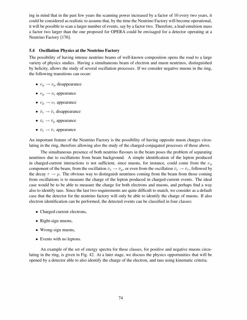
ing in mind that in the past few years the scanning power increased by a factor of 10 every two years, itcould be considered as realistic to assume that, by the time the Neutrino Factory will become operational,it will be possible to scan a larger number of events, say by a factor two. Therefore, a lead-emulsion massa factor two larger than the one proposed for OPERA could be envisaged for a detector operating at aNeutrino Factory [176].

5.4 Oscillation Physics at the Neutrino FactoryThe possibility of having intense neutrino beams of well-known composition opens the road to a largevariety of physics studies. Having a simultaneous beam of electron and muon neutrinos, distinguishedby helicity, allows the study of several oscillation processes. If we consider negative muons in the ring,the following transitions can occur:

• νµ → νµ disappearance

• νµ → νe appearance

• νµ → ντ appearance

• νe → νe disappearance

• νe → νµ appearance

• νe → ντ appearance

An important feature of the Neutrino Factory is the possibility of having opposite muon charges circu-lating in the ring, therefore allowing also the study of the charged-conjugated processes of those above.

The simultaneous presence of both neutrino flavours in the beam poses the problem of separatingneutrinos due to oscillations from beam background. A simple identification of the lepton producedin charged-current interactions is not sufficient, since muons, for instance, could come from the νµ

component of the beam, from the oscillation νe → νµ, or even from the oscillation νe → ντ , followed bythe decay τ → µ. The obvious way to distinguish neutrinos coming from the beam from those comingfrom oscillations is to measure the charge of the lepton produced in charged-current events. The idealcase would be to be able to measure the charge for both electrons and muons, and perhaps find a wayalso to identify taus. Since the last two requirements are quite difficult to match, we consider as a defaultcase that the detector for the neutrino factory will only be able to identify the charge of muons. If alsoelectron identification can be performed, the detected events can be classified in four classes:

• Charged-current electrons,

• Right-sign muons,

• Wrong-sign muons,

• Events with no leptons.

An example of the set of energy spectra for these classes, for positive and negative muons circu-lating in the ring, is given in Fig. 42. At a later stage, we discuss the physics opportunities that will beopened by a detector able to also identify the charge of the electron, and taus using kinematic criteria.

74

Eµ = 30 GeV, L = 7400 km, 1020 µ- decays

0

20

40

60

80

100

120

0 5 10 15 20 25 30 35 40Evisible (GeV)

dN/d

Eν

(νe

CC

eve

nts/

1.6G

eV p

er 1

0 kt

on)

Anti-νe+νe+ντ CCAnti-νe CCνe CCντ CC

Eµ = 30 GeV, L = 7400 km, 1020 µ- decays

0

10

20

30

40

50

60

0 5 10 15 20 25 30 35 40Evisible (GeV)

dN/d

Eν

(νµ

CC

eve

nts/

1.6G

eV p

er 1

0 kt

on)

νµ + ντ CC + backgroundνµ CCντ CCBackground

Eµ = 30 GeV, L = 7400 km, 1021 µ+ decays

0

20

40

60

80

100

120

140

160

180

0 5 10 15 20 25 30 35 40Evisible (GeV)

dN/d

Eν

(νµ

CC

eve

nts/

1.6G

eV p

er 1

0 kt

on)

νµ + ντ CC + backgroundνµ CCντ CC

Background

Eµ = 30 GeV, L = 7400 km, 1020 µ- decays

0

20

40

60

80

100

0 5 10 15 20 25 30 35 40Evisible (GeV)

dN/d

Eν

(ν e

vent

s/1.

6GeV

per

10

kton

)

ν NC + ντ CCν NCντ CC

Fig. 42: The four classes of events that can be studied in a detector with electron and muon charge identification.

From the top, left to right: events with high-energy electrons, right-sign muons, wrong-sign muons and no charged

leptons [78].

75

5.4.1 Precision measurements of oscillations

The first parameters to be measured are those governing the leading atmospheric oscillation νµ → ντ :θ23 and ∆m2

23. These parameters are mainly determined from the disappearance of muon neutrinos in thebeam, observed using right-sign muon events. The maximum of the oscillation probability will producea dip in the visible spectrum; the energy position of this dip will be correlated to the value of ∆m2

23, andthe depth to θ23. It is therefore favourable to choose an energy and baseline such that the maximum ofthe oscillation probability lies comfortably inside the detectable spectrum.

The precision on the measurement of the oscillation parameters has been addressed by severalgroups [163, 78, 172], and is normally performed by a fit of the energy spectra of the event classes (aspreviously said, this fit is largely dominated by right-sign muon events). As shown in Fig. 43, precisionsof the order of 1% on ∆m2

23 and of 10% on sin2 θ23 are foreseen.

Eµ = 30 GeV, L = 2900 km, 2 x 1020 µ decays

0.002

0.003

0.004

0.005

0.006

0.007

0.008

0.009

0 0.2 0.4 0.6 0.8 1sin2 Θ23

∆m2 23

(eV

2 ) Eµ = 30 GeV, L = 7400 km, 2 x 1020 µ decays

0.002

0.003

0.004

0.005

0.006

0.007

0.008

0.009

0 0.2 0.4 0.6 0.8 1sin2 Θ23

∆m2 23

(eV

2 )

Fig. 43: Measurement of the parameters of the leading oscillation [78].

5.4.2 Sensitivity to θ13

So far, the most accurate information we have on the angle θ13, i.e., the mixing of electron neutrinos andthe other two families (which are maximally mixed among themselves), is that sin2 2θ13 < 0.1 [14]. In afavourable case, a non-zero value of this parameter could be discovered before the Neutrino Factory byexperiments running in first-generation neutrino beams, such as ICARUS, OPERA and MINOS. Muchlarger sensitivity will however be achieved by super-beams, for instance the JHF-Super-Kamiokandeproject. Experiments performed in ‘conventional’ beams from pion decays will, however, always belimited by the presence of a νe component in the beam itself, representing an irreducible backgroundto the search for νµ → νe oscillations. It was first realized in [20] that the Neutrino Factory wouldhave a significantly improved sensitivity to θ13 from the measurement of the wrong-sign muon signal.This measures the oscillation νe → νµ, where the oscillated muon neutrinos are easily separated fromthe beam component of opposite helicity by measuring the charge of the produced muon. We havealready seen that the decays of charmed particles, kaons and pions can produce a background to thewrong-sign muon sample. Applying strong cuts on muon momentum and isolation, it was reported [116]that the background could be reduced by as much as a factor 106, keeping an efficiency of about 40%.An excellent background rejection with good efficiency could also be obtained using a hybrid emulsiondetector [176].

76

Pµ Qt

Pµ Qt

Fig. 44: Backgrounds and efficiencies for wrong-sign muons, for charged-current (upper plots) and neutral-

current (lower plots) events. We display the dependence on the cut on muon momemtum (left plots) and on the Qt

of the muon with respect to the hadronic jet (right plots) [116].

77

As in the previous case, the parameter θ13 is extracted from a fit to the energy distribution of thevarious classes, and in this case the fit is largely dominated by the wrong-sign muons. Moreover, from theformula of the oscillation probability we see that the value of θ13 has a limited influence on the spectralshape, and even factorizes out from the energy dependence in the approximation ∆m2

12 = 0, see (34), somost of the information actually comes from just counting wrong-sign muon events.

The background level is the ultimate limiting factor for this measurement, and pushing backgroundrejection to the high values quoted above allows one to reach sensitivities of the order of sin2 θ13 < 10−5

for the optimal intermediate baseline (see the right plot of Fig. 45). In the ideal case of no backgroundand 100% efficiency for the signal, almost another order of magnitude on the sensitivity could be gained(left plot of Fig. 45).

5107 106 5106 105 5105

sin2Θ13

0.001

0.002

0.003

0.004

0.005

0.006

m232

5107 106 5106 105 5105

sin2Θ13

0.001

0.002

0.003

0.004

0.005

0.006

m232

Fig. 45: Sensitivity to sin2 θ13 for a magnetized iron detector, in the case of no backround (left) and when a

realistic background is considered (right). The three lines correspond to baselines of 730 (dashed), 3500 (solid)

and 7300 km (dotted). Both plots were made assuming negligible effects of the solar parameters (i.e. for the small

angle or small ∆m212 solutions of the solar neutrino deficit) [116].

5.4.3 Matter effects

For practical reasons, long-baseline experiments can only be performed with neutrinos passing throughthe Earth. We know that electron neutrinos traversing matter interact with the electrons of the material,leading to a modification of the effective mixing matrix, and therefore of the oscillation probability, ina way which is asymmetric between neutrinos and antineutrinos. We have seen in section 2.2.3 thatthe oscillation probabilities including matter effects in the context of three-family oscillations are rathersimple when the solar mass difference, ∆m2

12, can be neglected.

According to (52), the oscillation probability νe → νµ has the same form as in vacuum (34) if θ13

is modified to:

sin2 2θm13(D) =

sin2 2θ13

sin2 2θ13 + ( D∆m2

23

− cos 2θ13)2(65)

and the effective atmospheric mass splitting is modified to

∆M223 ' ∆m2

23

√

sin2 2θ13 + (D

∆m223

− cos 2θ13)2. (66)

78

where

D = ±2√

2GF neE = 7.65 × 10−5eV 2(ρ

gcm−3)(

E

GeV),

with ne being the average electron density in the path crossed, ρ the average electron density, and thesign ± standing for neutrinos and antineutrinos, respectively. The quantity ∆m2

23 can also be positivein the case of a hierarchical spectrum or negative in the case of the inverted hierarchy. In the first case,the denominator of (65) is always larger than 1 for antineutrinos, and thus the effective angle is alwayssmaller than the vacuum one. For neutrinos, the resonance condition will be met for

D ' ∆m223 cos 2θ13,

for which value the effective angle becomes unity, no matter what the vacuum value was. It is thereforepossible to have large enhancements of the oscillation probability, around the resonance energy

Eres ≈ 1.32 × 104 cos 2θ∆m2(eV 2)

ρ(g/cm3).

Note however that the effective mass splitting at resonance decreases linearly with the vacuum value ofsin 2θ13, so, in order to get large probabilities, one needs to go to larger baselines for smaller sin 2θ13. Ifthe sign of ∆m2

23 is negative, the same reasoning applies, interchanging neutrinos and antineutrinos.

The asymmetry between neutrinos and antineutrinos due to the matter effect is a very effective wayto measure the sign of ∆m2

23, and establish the degenerate or hierarchical structure of neutrino masses.It has never been observed, and will be hard to detect with conventional super-beams, since it requiresthe comparison of runs with neutrinos and antineutrinos, and baselines larger than 1000 km. On theother hand, the crossing of such an MSW resonance is a plausible explanation for reconciling the largedisappearance of solar neutrinos from the Sun with the lack of a significant seasonal variation, as wouldbe expected from the eccentricity of the Earth orbit if the oscillation was taking place in the vacuum.Unfortunately, solar neutrino experiments cannot tell us anything about the sign of ∆m2

23.

Matter asymmetries on earth are relatively easy to detect at a Neutrino Factory [164, 165]. Al-though this is good news for the measurement of the sign of ∆m2

23, these asymmetries actually interferewith the measurement of leptonic CP violation, which is the most ambitious goal of this machine. Therelative amplitudes of the two effects as a function of the baseline can be seen in Fig. 46. It shows, ona logarithmic scale, the ratio of events that have oscillated into muon antineutrinos to events that haveoscillated into muon neutrinos, as a function of the baseline. The measurement of such a ratio requiresrunning the machine alternatively with positive and negative muons in the ring. The upper lines corre-spond to negative values of ∆m2

23, and the lower ones to positive values. The three lines are obtainedfor different values of the CP-violating parameter δ, that will be discussed in more detail in the nextsection, and the error bars correspond to statistical errors for a 40 kt detector after 1021 muon decays inthe ring for each muon charge. We see that the asymmetry due to matter effects is quite large, and caneasily be detected for baselines larger than about 1000 km. Matter effects and CP violation interfere, andone effect can mask the other, until baselines of about 2000 km. Above that distance matter effects arealways larger than CP violation, which is even completely cancelled for one particular distance around7500 km.

5.4.4 CP violation

Detecting the presence of a complex phase in the leptonic mixing matrix is one of the most ambitiousgoals of neutrino physics, and would justify the effort of building a neutrino factory [20, 166, 167, 168,116, 78]. In vacuum, we saw in (30) that the difference between the oscillation probabilities for thetransitions νe → νµ and νe → νµ can be written as

∆CP ∼ 1

2c13 sin 2θ12 sin 2θ13 sin 2θ23 sin δ[sin ∆12 sin∆13 sin∆23], (67)

79

0.001

0.01

0.1

1

10

100

1000

0 2000 4000 6000 8000 10000

1021 µsin22θ13 = 0.004

δm232 –

δm232 +

δ = 0°δ = 90°δ = −90°

L (km)

N(– ν e

→– ν µ

) / N

(νe→

ν µ)

Fig. 46: Ratio of the oscillation probabilities of neutrinos and antineutrinos as a function of the baseline. The

different lines correspond to values of the CP-violating phase δ of 0, 90 and −90. After about 1000 km, matter

effects dominate over CP violation, whose effects even go to zero at a particular baseline around 7500 km [165].

80

log10(sin2 2θ13)

Asy

mm

etry

10-1

1

10

-5 -4.5 -4 -3.5 -3 -2.5 -2 -1.5 -1

Fig. 47: The CP-violating asymmetry and its error as a function of θ13, for different values of ∆m212.

which shows that, for the large mixing angle solution of the solar deficit, it is suppressed only in theparameters ∆12 and θ13. Since the CP-even parts of the probabilities are always larger than the CP-odd parts, they dominate the number of events and thus the error on the measured asymmetry. Forsmall enough ∆12, these terms are approximately proportional to sin2 2θ13 and independent of ∆12

(they are driven by the atmospheric oscillation, i.e. the first term in (31)). Assuming Gaussian errors, thesignificance of CP violation will then be proportional to

∆CP√Nev

∝ sin 2θ13√

sin2 2θ13

∆12, (68)

and will not depend on θ13 [168], while it is linearly proportional to the small mass splitting. The factthat ∆12 is actually different from zero means that the subleading oscillation will become important andeventually dominate for small θ13. In this regime the role of sin 2θ13 and ∆12 are interchanged and thesignificance of the CP asymmetry is suppressed linearly in sin 2θ13 and approximately independent ofthe solar mass splitting

∆CP√Nev

∝ ∆12√

(∆12)2sin 2θ13. (69)

This is shown in Fig. 47, where the CP asymmetry at the maximum of the oscillation probability iscompared to its error (computed for a relatively modest neutrino flux) as a function of sin2 2θ13. We seethat the effect and the error decrease together with sin2 2θ13 until a value (that depends on ∆12) wherethe subleading oscillation becomes dominant, and the number of oscillated events goes to a constant evenfor very small θ13. In this regime the significance of the asymmetry decreases linearly with sin 2θ13.

A possible measurement of this asymmetry is given by the integrated asymmetry [20]:

ACPeµ =

N [µ−]/N0[e−]+ − N [µ+]/N0[e

+]−N [µ−]/N0[e−]+ + N [µ+]/N0[e+]−

, (70)

where the suffix defines the sign of the decaying muon, N [µ±] is the measured number of wrong-signmuons and N0[e

∓] the expected number of νe and νe charged-current interactions in the absence of os-cillations. The statistical significance of the asymmetry, i.e., the asymmetry divided by its error, assumed

81

0 2000 4000 6000 8000 10000L @kmD0

200

400

600

800

AC

PHΠ2LD

AC

P

totalbin1bin2bin3bin4bin5

Fig. 48: The significance of the CP asymmetry as a function of the baseline [116]. On the left, the asymmetry

is just the matter-induced asymmetry (SMA solution parameters). On the right we show, for LMA parameters, a

subtracted asymmetry directly measuring δ.

to be Gaussian, in vacuum is proportional to [167]

ACP

∆ACP∝

√E

∣

∣

∣

∣

sin

(

∆m223L

4Eν

)∣

∣

∣

∣

. (71)

This is maximal at the peak of the atmospheric oscillation.

These considerations, valid in vacuum, get however modified by matter effects, as already seenin Fig. 46. In matter, very large asymmetries are created by the MSW effect. The left plot of Fig. 48shows the total asymmetry in matter as a function of the baseline, while the one on the right shows theasymmetry obtained after subtracting the matter-induced asymmetry for δ = 0. Clearly the significanceof the matter-induced asymmetry and the intrinsic one peak at different baselines.

Although the right plot shows that for the parameters in the LMA range, intrinsic CP violationshould be measurable at distances O(3000) km, this analysis assumes only experimental errors and not‘theoretical’ ones. Given that the matter-induced asymmetry depends very sensitively on the oscillationparameters, mainly θ13, θ23 and ∆m2

23 as well as on the Earth matter density, it is very important toclarify whether the expected uncertainties in those ‘theoretical’ parameters will be small enough not towash out the effect.

Concerning the atmospheric parameters |∆m223| and sin2 2θ23, we have seen that they can be

measured with very good precision using disappearance measurements at the neutrino factory. It wasshown [76] that the knowledge of the precise profile of the matter density along the neutrino path isnot very relevant, but for a neutrino experiment only the knowledge of the mean value is needed. Thisaverage density can probably be known with 5% accuracy [169], or even directly measured with a 10%precision [78].

On the other hand the angle θ13 as well as the discrete choices of the sign of ∆m223 and cos θ23 if

θ23 6= π/4, will have to be determined simultaneously using the wrong-sign muon signals. The analysishas to be refined to include these unknowns and, as we will see in the next sections, this will reveal theexistence of

• Strong parameter correlations: mainly between θ13 and δ [116],

• Degenerate solutions [117, 171].

82

0

1000

2000

3000

4000

5000

6000

7000

0 10 20 30 40Evis (GeV)

Eve

nts/

1.6

GeV

Electrons

-35

-30

-25

-20

-15

-10

-5

0

0 10 20 30 40Evis (GeV)

Eve

nts(

δ=π/

2-δ=

0)/1

.6 G

eV0

20406080

100120140160180

0 10 20 30 40Evis (GeV)

Eve

nts/

1.6

GeV δ=π/2

δ=0

Wrong-sign muons

-5

0

5

10

15

20

0 10 20 30 40Evis (GeV)

Eve

nts(

δ=π/

2-δ

Fig. 49: Left plots: number of oscillated events for δ = 0 (black histogram) and δ = π/2 (red histogram). The

right plots represent the difference of the two, for νµ → νe and νe → νµ transitions, respectively. If the difference

is similar, the signal in the electron channel is invisible due to the vey large background. In the muon channel, we

notice the the shift of the oscillation maximum generated by CP violation [78].

In order to minimize and resolve these, it is important to use all the spectral information available andchoose appropiately the baseline. Fig. 49 shows the energy dependence of the intrinsic effect of δ 6= 0.In the global fit of course we consider the wrong-sign muon signals for both µ+ and µ− and not only theCP asymmetries, since also the CP-even parts contain very valuable information on the unknowns.

5.4.5 Correlations and choice of baseline

Due to the small energy dependence induced by CP violation, the use of spectral information to have asimultaneous measurement of δ and θ13 is not very effective, and only helps under some conditions. Infact, the first simultaneous fits of θ13 and δ perfomed in [116, 78] revealed for most of the cases a strongcorrelation between the two parameters, which was more important at shorter baselines, see Figs. 50 and51. The reason for this is easy to understand. The neutrino and antineutrino oscillation probabilities invacuum (30), have the following dependences on θ13 and δ:

P (νe → νµ)P (νµ → νe) = A sin2 2θ13 + B sin 2θ13 cos δ ± C sin 2θ13 sin δ + D (72)

where the coefficients A,B,C,D depend on the energy, baseline and the remaining oscillation parame-ters. In matter a similar structure is found, though the coefficients are different for neutrinos and antineu-trinos and depend also on the earth matter density. In the limit of large Eν or small L (∆12 < ∆23 1),the coefficients A,B and D have the same energy dependence, while C is suppressed by an extra factor∆23 compared to the others. This is so both in vacuum and in matter, because matter effects are irrelevant

83

in this limit. In this situation it is clear that the measurements of the oscillation probabilities for neutrinosand antineutrinos give information on the same combination of the two unknowns: θ13 and δ

A sin2 2θ13 + B sin 2θ13 cos δ + D, (73)

resulting in the strong correlation [116] that can be nicely seen in the left plot of Fig. 57, at a baselineof L = 732 km. Even though the spectral information has been used for this baseline, it is only relevantin the low-energy region. The same fit performed with a lower energy threshold in Fig.51 shows thatcorrelations are smaller, but still present. As the baseline is increased the CP-odd term, i.e., the coefficientC , grows and the neutrino and antineutrino probabilities measure two independent combinations of thetwo parameters. Also the energy dependence in the accessible energy range becomes more important.Indeed, the fits at L = 3500 km in Fig. 50 and at L = 2900 km in Fig. 51 show that δ and θ13 can bedisentangled. At even larger baselines, sensitivity to δ is lost.

How much can the neutrino energy threshold actually be lowered in order to reduce correlations,using spectral information in the important low-energy region? The answer to this question depends ofcourse on the detector, but since we want to discriminate the oscillation signal from a constant back-ground, also on the amplitude of the oscillation signal, i.e., on the oscillation parameters. For smallvalues of θ13, the good purity needed to discriminate the wrong-sign muon signal from background re-quires very hard cuts on the muon momentum, and therefore the loss of the most interesting part of theneutrino spectrum. For instance, a magnetized iron detector can in principle reach background rejectionfactors of the order of 106, but at the price of an effective cutoff on neutrino energies of about 10 GeV.

The conclusion of this study was that in the case of one baseline, the optimal choice to study CPviolation was in the intermediate range L = O(3000) km for a machine of Eµ = 30 − 50 GeV [116].

All the above considerations pointing to the optimal distance of O(3000)km have assumed a con-stant beam flux. It is possible to argue that a lower-energy machine could profit from savings on theaccelerator and provide a larger flux than a high-energy one. If we assume that, for various possible Neu-trino Factory designs, the flux can be inversely proportional to the beam energy (in other words, the totalbeam power is constant), this fact compensates the linear sensitivity growth, and it can be shown [75] thatall energy/baseline combinations that keep constant the ratio of these two quantities are equivalent, witha slight preference for the lower energy-baseline combinations, due to the smaller influence of mattereffects. This study assumes a neutrino energy threshold of 2 GeV, for which a baseline of 732 km and amaximal neutrino energy of 7.5 GeV are slightly better than a baseline of 2900 km and an energy of 30GeV, if the flux of the first case is 4 times larger than the second one. However, a coarse detector withlarger energy thresholds will always benefit from a longer baseline and higher neutrino energy [172].

Correlations of the phase δ with other oscillation parameters have also been studied in severalworks [173, 117, 172, 174, 78]. The main conclusions are:

• The parameters of the leading oscillation will be measured independently by the Neutrino Factoryitself using the same-sign muon sample, and the precision reached will be much superior thanthat producing any sizeable systematic effect on the measurement of δ. An exception are signand octant ambiguities, that can produce degenerate solutions, and will be discussed in the nextsection.

• Knowledge of the parameters governing solar neutrino oscillations (θ12 and ∆m12) is essential, butthe indications are that KamLand results should be precise enough to reduce to negligible levelsthe impact of the uncertainties on these measurements to the determination of δ.

• The average earth density can probably be known up to 5% using geophysical techniques [169];however, a precision at least a factor 2 better would be desirable.

84

Fig. 50: Correlations in a simultaneous fit of θ13 and δ, using a neutrino energy threshold of about 10 GeV. Using

a single baseline correlations are very strong, but can be largely reduced by combining information from different

baselines and detector techniques [116].

85

0.04

0.0425

0.045

0.0475

0.05

0.0525

0.055

0.0575

0.06

0 0.5 1 1.5 2 2.5 3

L=732 kmδ13

sin2 2

Θ13

(68% C.L.)

(90% C.L.)

(99% C.L.)

L=2900 kmδ13

sin2 2

Θ13

(68% C.L.)

(90% C.L.)

(99% C.L.)0.04

0.0425

0.045

0.0475

0.05

0.0525

0.055

0.0575

0.06

0 0.5 1 1.5 2 2.5 3

Fig. 51: Contours in the sin2 2θ13−δ plane assuming very low energy threshold (2 GeV muon energy) at distances

of 732 or 2900 km. Even if not as pronounced as in the case of the previous plot, done with much higher neutrino

energy thresholds, the short baseline starts to show correlations between the two parameters [78].

86

5.4.6 Degeneracies

We have seen in the previous section that it is very hard to disentangle θ13 and δ at short baselines ofO(1000) km, because the neutrino and antineutrino probabilities are sensitive to approximately the samecombination of the two parameters. At larger baselines the correlation is resolved thanks mainly to thelarger sin δ term in (73). However, even in this case, the impossibility of measuring precisely the energydependence of the wrong-sign muon signals can result in the existence of degenerate solutions for theθ13 and δ, i.e., disconnected areas of the parameter space that lead to experimentally indistinguishablesignatures [117]. The origin of this is that, at fixed neutrino energy and baseline, the equations

Pνeνµ(θ′13, δ′,Θ′) ' Pνeνµ(θ13, δ,Θ)

Pνeνµ(θ′13, δ′,Θ′) ' Pνeνµ(θ13, δ,Θ) (74)

have more solutions than the true one: θ ′13 = θ13 and δ′ = δ. We use the symbols Θ and Θ′ to denote theother sets of oscillation parameters. The reason why in general Θ′ might be different from Θ is due tothe discrete ambiguities of the type sign(∆m2

23) and sign(cos θ23). The three main types of degeneraciescorrespond to different choices of Θ′:

• Intrinsic, when Θ′ = Θ, so all other parameters are the same, but the conditions (74) are satisfiedfor sets of θ13, δ different from the true one [117].

• The sign of ∆m213 is different in the two sides of the equations (74) [171]. In vacuum, a change of

sign of ∆m213 is approximately equivalent to the substitution δ → π − δ [170].

• The value of θ23 on the left side of (74) is π/2 − θ23 of that on the right side [171]. The fakesolutions obviously collapse to the intrinsic ones for maximal mixing: θ23 = π/2.

An example of intrinsic degeneracies is shown in Fig. 52, obtained for a simultaneous fit of θ13, δin a large magnetised iron detector. The true values of the parameters are indicated by the stars, while afit to the observed data would find several disconnected regions. These plots were made for a baseline of2800 km.

Fig. 52: Simultaneous fits of δ and θ13 at L = 2800 km, for θ13 = 2 (left) and 8 (right). True values are

indicated by stars, and many degenerate solutions are present [117].

Degeneracies can be a very serious source of uncertainties in the determination of the parameters.If, for instance, we define (conservatively) the sensitivity to sin2 2θ13 as the largest value of sin2 2θ13

87

which can be fit to sin2 2θ13 = 0, we will find that the degenerate solution can be interpreted as anadditional uncertainty which makes it almost impossible to push the sensitivity to sin2 2θ13 much below10−3 [175] (see Fig. 53).

10-6 10-5 10-4 10-3 10-2 10-1

sin2 2Θ13

Sensitivity to sin22Θ13

SystematicCorrelationDegeneracy

JHF-SK

NuMI

JHF-HK

NuFact-I

NuFact-II

10-6 10-5 10-4 10-3 10-2 10-1

sin2 2Θ13

Sensitivity to sin22Θ13

Fig. 53: Limitations on the achievable sensitivity to sin2 2θ13 for various assumptions on future experiments,

which are described in [175]. The sensitivity to sin2 2θ13 is defined as the largest value of sin2 2θ13 which can be

fit to sin2 2θ13 = 0, which means that the degenerate solutions enter as an additional source of uncertainties. In

this interpretation, the importance of resolving the degeneracies from the combination of various experiments is

very clear.

There are fortunately several handles to deal with these degeneracies. The position of the fakesolutions is very sensitive to the value L/E and the presence or not of matter effects. The first possibilityis then to have two baselines at the Neutrino Factory, since combining the information of two experimentsallows the exploration of a different L/E regime, and matter effects behave differently at two baselinesfor the disconnected sets of parameters. We see from Fig. 54 that the combination of the intermediateand the very long baseline eliminates all degeneracies. The combination of the intermediate and a shortbaseline, e.g., 732 km is not so good, because of the strong correlations present in the shorter baseline.

If a baseline of the order of 732 km is used in addition to one around 3000 km, it is more interestingto consider at the shorter baseline a detector with capabilities to detect τ ’s from νe → ντ oscillations. Themeasurement of this transition would be a great help in resolving degeneracies, since the two processesνe → νµ and νe → ντ give complementary information[176]. In fact, the formulae for oscillationprobabilities in vacuum of these processes are very similar: the νe → ντ probability can be obtainedfrom (34) by swapping s2

23 ↔ c223 and changing the sign of the δ−dependent terms. In Fig. 55, we plot

the curves of equal νe → νµ and νe → ντ probabilities in the (∆θ13 ≡ θ′13−θ13, δ′) plane for some fixedvalues of the true parameters: θ13 = 5, δ = 90. The different curves correspond to different energybins. The curves all meet only at the true values of the parameters: δ ′ = 90 and ∆θ = 0, while allthe curves for the wrong-sign muons are approximately degenerate. This illustrates the potential of thecombination of golden and silver events to exclude the fake solutions.

In [176] a detailed study of a realistic experimental setup has been presented. The detector con-sidered is an OPERA-like hybrid with lead and emulsion [160]. It has been shown that the τ vertexrecognition in the emulsion detector allows one to separate νe → ντ from νe → νµ muon events, and

88

Fig. 54: For a wide choice of the parameters, in order to reduce correlations in a simultaneous fit to θ13 and δ,

the combination of the intermediate and the very long baseline is preferred over that of the short and intermediate

baselines [117].

to reduce strongly the effect of the charm decay background. The outcome of this study is that a 4 ktdetector at L = 732 km in combination with the 40 kt magnetised iron detector at L = 3000 km wouldsolve the intrinsic ambiguity for θ13 ≥ 1 and any value of δ.

Another interesting approach to resolve degeneracies is the combination of information from theNeutrino Factory and a super-beam [177]. The synergy of the super-beam project with the NeutrinoFactory has already been discussed from the point of view of the accelerator infrastructure, since we sawthat several components needed for building a super-beam are the same as those for the Neutrino Factory.Most likely, at the time of the operation of this facility, results from the super-beam will already beavailable, and the synergy between the two projects will emerge in the physics. Due to the very differentL/E regime - super-beams are designed to operate around the oscillation maximum - and matter effects- which are much smaller for super-beams due to the shorter baseline, the knowledge of the super-beamresults will help resolve the degeneracies.

Sufficiently powerful super-beams can search for CP violation in a favourable corner of the pa-rameter space. It was shown [177] that a combination of the results from the proposed CERN-Frejussuper-beam and a Neutrino Factory with a single baseline could eliminate almost completely all degen-eracies. The reason is easy to understand from Fig. 56: the fake solutions, present in both experiments,appear in different areas of the parameter space, and therefore are excluded once the experiments arecombined.

Combined with the results of the super-beam, even the baseline of 732 km, normally too short togive definitive results on its own, can provide good measurements of the oscillation parameters. Thisis shown by the contours in the plane (θ13, δ) in Fig. 57. We already saw that a high-energy NeutrinoFactory coupled with a detector with high threshold for neutrino detection reaches its maximal sensitivityfor a baseline of about 3000 km. For a shorter baseline, the experiment measures only the combination(73) as we already discussed (left plot in Fig. 57). The addition of the super-beam information, whichalso is not able to resolve the degeneracies on its own, leads to a very good determination of the twoparameters as shown in the right plot of Fig. 57.

This result is extremely important for the definition of the Neutrino Factory design itself. It iscommon belief that an intermediate baseline of about 3000 km is the best compromise between being

89

−2 −1 0 1 2 ∆θ

−180

−90

0

90

180

δ

"golden" events

"silver" events

Fig. 55: Curves of equal oscillation probability in the δ, ∆θ plane (where ∆θ is the difference between θ13 and

its nominal value of 5), for νe → νµ and νe → ντ . We see that these curves, generated for different energy bins,

all meet at the nominal value of the parameters [176].

long enough to have the maximum of the oscillation at sufficiently high energy, and not too far not tohave the CP violation suppressed by matter effects. Since a low-energy super-beam will probably bebuilt before the Neutrino Factory, the energy/baseline optimization of the latter will have to take intoaccount the combination with the super-beam results.

5.4.7 T violation

The problem of the neutrino-antineutrino asymmetry generated by matter effects acting as a backgroundto CP violation could be solved if, instead of the CP asymmetry, we could measure the T asymmetry, i.e.,the difference in oscillation probability between the processes νe → νµ and νµ → νe. This is in principlepossible at the Neutrino Factory, since if the machine is operated with two different beam polarities,both processes (and even their complex conjugates) occur. The problem is that, in order to discriminateoscillated events from the beam component of the same flavour, the charge has to be measured for bothleptons. While this is possible in a relatively straightforward way for muon final states, the measurementof the electron charge is much more complicated, due to the early formation of electromagnetic showers.The possibility of measuring the electron charge has been studied [75] for a magnetised liquid argondetector. A charge confusion at the per mille level with an efficiency of about 10% for electrons of lessthan 5 GeV energy should be reached with values of the magnetic field exceeding 1 Tesla. In that case,it would be possible to measure directly the two T-conjugated oscillation probabilities, and detect thedifference between the two (see Fig. 58) with a statistical significance similar to that of the CP violation.Due to the impossibility of detecting the charge of high-energy electrons with realistic values of themagnetic field, an experiment looking for T violation would require a low-energy, high-intensity muonbeam.

90

0

0.5

1

1.5

2

0.1 1 10

θ’ 13-θ

13(d

eg)

θ13(deg)

δ= 90o

NF-732 kmNF-2810 km

JHFSPL

0

50

100

150

200

250

300

350

0.1 1 10

δ’ (d

eg)

θ13(deg)

δ= 90o

NF-732 kmNF-2810 km

JHFSPL

Fig. 56: Values of θ′13 − θ13 (left) and δ′ (right) for the intrinsic fake solution for δ = 90. We see that fake

solutions, albeit present for all kinds of experiments, appear for different values of the parameters, and therefore a

combination of experiments allows one to exclude them [177].

Fig. 57: Simultaneous measurements of θ13 and δ and of the CP-violating phase δ. The left plot is produced using

only the information from a Neutrino Factory with an iron magnetised detector placed at 732 km: there are clear

correlations between the parameters and degenerate solutions. In the right plot, the Neutrino Factory is combined

with the results from the super-beam, and both correlations and degeneracies disappear [177].

91

1021 muons for L = 732 km

-0.03

-0.02

-0.01

0

0.01

0.02

0.03

0.04

0 2.5 5 7.5

δ = π/2

Eν (GeV)

∆ T

-0.03

-0.02

-0.01

0

0.01

0.02

0.03

0.04

0 2.5 5 7.5

δ = 0

Eν (GeV)

∆ T

-0.03

-0.02

-0.01

0

0.01

0.02

0.03

0.04

2.5 5 7.5

δ = - π/2

Eν (GeV)

∆ T

-0.03

-0.02

-0.01

0

0.01

0.02

0.03

0.04

0 2.5 5 7.5

δ = π/2

Eν– (GeV)

∆– T

-0.03

-0.02

-0.01

0

0.01

0.02

0.03

0.04

0 2.5 5 7.5

δ = 0

Eν– (GeV)

∆– T-0.03

-0.02

-0.01

0

0.01

0.02

0.03

0.04

2.5 5 7.5

δ = - π/2

Eν– (GeV)

∆– T

Figure 18: Direct T -violation: Binned ∆T (i) discriminant for neutrinos (upper plots)and antineutrinos (lower plots) for three values of the δ-phase: δ = +π/2, δ = 0 andδ = −π/2. The errors are statistical and correspond to a normalization of 1021 muondecays and a baseline of L = 732 km. A 20% electron efficiency with a charge confusionprobability of 0.1% has been assumed. The change of sign of the effect with respect ofthe change δ → −δ and the substitution of neutrinos by antineutrinos is clearly visible.The full curve corresponds to the theoretical probability difference.

51

Fig. 58: Oscillation probabilities for T-conjugate processes measured with a 10 kt detector with electron charge

identification capabilities. The error bars correspond to 1021 muons decays, for an electron charge efficiency of

20% and misidentification of 0.1% [75].

5.4.8 Search for νe → ντ

We saw in the previous section that the detection of τ leptons could be useful in resolving the degen-eracies in the search for CP violation, due to the different behaviour of the δ−dependent term in theoscillation probability. The detection of taus, both from νµ → ντ and νe → ντ oscillations, is alsoextremely important as a test of the unitarity of the mixing matrix. Comparing the yields from thesechannels to those expected from the disappearance, it is possible to put strong limits on the conversionof neutrinos into another species, for instance sterile neutrinos. If we call α and β the ratios of the oscil-lation probabilities νµ → ντ and νe → ντ with respect to their expected value, the precisions on theseparameters, with the assumptions made in [78], are shown in Table 11.

Baseline ∆α/α ∆β/β

2900 2% 25%7400 2% 20%

Table 11: Precision in the determination of the parameters α and β, that quantify the amount of νµ → ντ and

νe → ντ present in the data [78].

5.5 Search for New Physics at the Neutrino Factory

As discussed earlier, it is not possible to accommodate all the present experimental results within thestandard three-family oscillation framework. Up to now, we have assumed that the unconfirmed resultfrom LSND could be explained by some misunderstood experimental effect, rather than by neutrinooscillations. We have already commented that Neutrino Factory physics would be even richer if theLSND result is indeed due to neutrino oscillations.

92

If the effect is due to some other interactions violating lepton flavour, distinct from neutrino oscil-lations, again the Neutrino Factory would be the ideal machine to study them. Because of the shape ofthe produced neutrino spectrum, this machine would also be an ideal place to look for a modification ofthe MSW potential for matter oscillations, since these effects would mainly be visible in the high-energypart of the spectrum.

Discussions of these two possibilities are presented in the following two subsections. We notealso that a deviation from the standard Lorentz metric due to extra dimensions could be explored bydeviations of the neutrino velocity from the speed of light, which could in principle be measurable if oneequipped a far detector with RPCs having a time resolution around 200 ps [181].

5.5.1 New physics in short-baseline experiments

The search for lepton-number-violating (LNV) muon decays with ∆L = 2, of the type:

µ− → e− + νe + ν` (75)

where (` = e, µ, τ), would be possible by looking for wrong-sign electrons, which would produce thefollowing standard charged-current weak interactions in the detector:

νe + N → e− + X (76)

ν` + N → l− + X. (77)

We assume that µ− are circulating in the ring, since the signature sought has two neutrinos with negativehelicity in the final state, so that one profit from the enhanced cross sections, compared with the positive-helicity case.

The signal for such anomalous muon decays does not depend on the distance between the neutrinosource and the detector, unlike the oscillation case, and therefore is better studied with relatively smalldetectors at short distances, where one benefit from the higher neutrino flux. A 10 ton fiducial massLiquid Argon detector located at a distance of 100 m from the muon storage ring was considered in [182]as a realistic case.

Because the signal sought consists in the appearance of final-state electrons, while standard eventshave positrons in the final state, an experiment with electron charge discrimination is mandatory. Thisis an experimental challenge, given the short radiation length in liquid argon. Realistic efficiencies andexperimental backgrounds in a detector with the characteristics of the ICARUS Liquid Argon imagingTPC[183] have been studied. The detector simulated was a medium-sized Liquid Argon vessel sur-rounded by a dipole magnet.

Table 12 shows the effects of the cuts applied for a normalization of 1019 muon decays. Tocompute the expected number of signal events, a branching probability of 2.5 × 10−3 was considered,compatible with the LSND excess.

Given the low muon energies considered, most of the events will be quasi-elastic. Therefore, afinal state configuration containing an electron and a reconstructed proton and no additional hadronicparticles is required. These criteria reduce the quas-ielastic background (where we expect a neutronrather than a proton in the final state) by almost three orders of magnitude, while keeping more than50% of the signal. The neutral-current background, where electron candidates come from π0 conversion,is in general soft. After a cut on the electron candidate momentum, this kind of background becomesnegligible. Preliminary studies indicate that, for a Liquid Argon detector inside a 1 T magnetic field, afit to the direction of the electromagnetic shower could provide a good determination of the charge ofleading electrons. Table 12 shows that applying loose criteria in the determination of the lepton chargeis enough to eliminate νe charged-current background.

93

Cuts νe CC νe CC

Eµ− = 2 GeV

Initial 540 62500One proton 367 11000No pions 323 100

Ee > 1 GeV 103 17Candidate charge 21 0.4

Eµ− = 5 GeV

Initial 5290 802000One proton 3390 212160No pions 2112 495

Ee > 3 GeV 351 163Candidate charge 71 4

Eµ− = 1 GeV

Initial 76 6300One proton 53 529No pions 48 8

Ee > 0.2 GeV 43 4Candidate charge 10 0.1

Table 12: The effects of cuts on background and signal. We assumed a negative muon ring energy Eµ− of 1, 2 and

5 GeV and a total of 1019 standard decays. The detector was assumed to be located 100 m from the center of the

straight section. The lepton-number-violating decay was assumed to have the branching probability 2.5 × 10−3.

We denote by Ee the energy of the identified electron in the event.

5.5.2 New physics in long-baseline experiments

Exotic physics effects may appear in neutrino production, neutrino interactions or neutrino propagationin matter. Whilst the first two cases are better studied in a near detector, benefiting from the higher flux,the effects of new physics on matter propagation are better observed in a long-baseline experiment, andmight even interfere in the interpretation of long-baseline oscillation experiments.

We recall that the standard MSW effect gives rise to diagonal contributions to the neutrino squared-mass matrix proportional to the neutrino energy. A flavor-changing neutrino interaction would give riseto a non-diagonal term which, although smaller than the diagonal ones, would also grow with the neutrinoenergy. The effective neutrino squared-mass matrix M 2

eff would become

M2eff = U

0 0 00 ∆m2

21 00 0 ∆m2

31

U † + 2EV

1 + εee εeµ εeτ

εµe εµµ εµτ

ετe ετµ εττ

, (78)

where E is the neutrino energy, U is the neutrino mixing matrix in the usual parameterization, and∆m2

21 > 0 is the smaller squared-mass difference. In the standard case, all the ε parameters are equal tozero.

A model-independent limit on ετµ can be inferred from atmospheric neutrino data [11]: ετµ<∼

0.05. Significant limits on the single εe,u,d quantities can be obtained if one assumes that the new physicsoperators originate from SU(2)W -invariant operators. Then experimental bounds on charged-lepton pro-

94

cesses imply [184, 185, 186]

εeµe

<∼ 10−6 εeτµ

<∼ 3 · 10−3 εeτe

<∼ 4 · 10−3 (79)

εu,dµe

<∼ 10−5 εu,dτµ

<∼ 10−2 εu,dτe

<∼ 10−2 . (80)

Since SU(2)W is broken, the limits above can be evaded. In the case of the exchange of a SU(2)W

multiplet of bosons with SU(2)W breaking masses [185, 186], the the SU(2)W breaking masses canrelaxed the limits by a factor of about 7, without a conflict with the electroweak precision data.

In general, the interactions involving the third family are far less constrained than those involvingthe first two. The constraint on εµe is so strong that no neutrino experiment would be able to improve it,since even at the limit the contribution it gives to neutrino oscillation is negligible. On the other hand,a value of ετe close to the experimental bound affects in a significant way both νe → νµ and νe → ντ

oscillations, as seen in Fig. 59.

10-5

10-4

10-3

10-2

0 5 10 15 20 25 30 35 40 45 50E (GeV)

P(ν

e→ν µ)

E (GeV)

P(ν

e→ν

µ)

10-7

10-6

10-5

10-4

10-3

0 5 10 15 20 25 30 35 40 45 50

Fig. 59: The νe → νµ oscillation probability in

the standard MSW model (full line) and in the pres-

ence of flavour-changing interactions (dashed line),

for sin2 2θ13 = 0.001 and ετe = 0.07 [188].

10-5

10-4

10-3

10-2

0 5 10 15 20 25 30 35 40 45 50E (GeV)

P(ν

e→ν τ)

E (GeV)

P(ν

e→ν

τ)

10-7

10-6

10-5

10-4

10-3

10-2

0 5 10 15 20 25 30 35 40 45 50

Fig. 60: The νe → ντ oscillation probability in

the standard MSW model (full line) and in the pres-

ence of flavour-changing interactions (dashed line),

for sin2 2θ13 = 0.001 and ετe = 0.07.

The probability for oscillation into muons gets multiplied by an almost energy-independent factor.The presence of new physics leads to confusion with the case of normal oscillations, and an experimentcould be led to infer a value of sin2 2θ13 higher than the true quantity [187]. However, the strong riseof the νe → ντ probability, a clear indication of the presence of nonstandard interactions, can be seenfrom the decay τ → µ, even with a detector only able to measure the muon momentum. The spectralshape of the muons will be so different that it is possible to distinguish the case of normal oscillationfrom those of new physics in large region of the parameter space [188], inferring the value of θ13 fromevent counting, and then comparing the observed spectrum with the theoretical one for the estimated θ13.It has been shown that, for sin2 2θ13>∼10−3, or ε13>∼10−2, the spectral differences are such that the twocases can be clearly separated.

95

6 SUMMARY AND OUTLOOK

Neutrino physics has been making great strides during the past few years. It has provided us with aunique window on physics beyond the Standard Model, and significant progress has recently been madein measuring the parameters of neutrino oscillations. The atmospheric mixing angle θ23 seems to be nearmaximal, and a large value of the solar mixing angle θ12 is now also favoured. These notable differencesfrom the small mixings observed previously among quarks whet our appetites for further information onneutrino oscillations. These may cast light on fundamental aspects of physics at the grand unificationscale where all the interactions may be unified. Just as the past generation has witnessed the establish-ment of the Standard Model and quark physics, neutrinos and physics beyond the Standard Model seemdestined to be at the forefront of experimental and theoretical physics for the coming generation.

Experiments now underway or being prepared will advance our knowledge of neutrino massesand oscillations in many ways. They will have improved sensitivity to neutrino masses and neutrinolessdouble-β decay. They will establish whether solar neutrino oscillations occur in the LMA, LOW, SMA orVAC region of parameters. They will clarify whether the LSND anomaly is due to neutrino oscillations.They will presumably confirm the existence of oscillation patterns, and that atmospheric νµ oscillatemainly into ντ . They will provide more precise measurements of the solar and atmospheric neutrinooscillation parameters, including the mass-squared differences, θ12 and θ23. They will have improvedsensitivity to θ13.

The neutrino physics communities in Europe, Japan and the United States are all consideringactively their options for the following step in oscillation physics. These should be addressed towardsthe many questions that are unlikely to be resolved in the approved round of experiments. These includepinning down θ13, seeing intrinsically three-generation effects in mixing, searching for CP violation, andfixing the sign of ∆m2

23 via matter effects. Short-term options include a JHF neutrino beam in Japan andoff-axis long-baseline experiments in the United States and Europe. Specific experiments can be devisedwhich address many of the individual open questions, but there is no guarantee that any or all of themwill be answered by this next round.

We have presented in this report a set of options for Europe that would provide powerful tools foraddressing all the open questions, by providing forefront experimental possibilities.

• A first step could be an intense proton source at CERN, the SPL, that would provide a low-energyneutrino beam of unprecedented power. This study also includes a summary report on the SPLdesign. The Frejus tunnel is at just the right distance to observe oscillation effects with an SPLbeam, and placing there a megaton-class water Cerenkov detector such as UNO would be anattractive option. The SPL-UNO combination would have a chance of observing CP violation inneutrino oscillations.

• A second possibility that has emerged from this study group is the concept of β beams, comingfrom the decays of radioactive isotopes produced by the SPL. Many accelerator questions vital forthe viability of this concept remain to be investigated, but it may provide an exciting alternativeoption for studying CP violation in neutrino oscillations, and has interesting synergies with otheroptions considered here.

• The best long-term option for neutrino physics is the neutrino factory based on muon decays ina storage ring. This offers unequalled reach for all the basic open questions: the magnitude ofθ13, CP violation and matter effects. Several important questions about the design of a neutrinofactory remain to be answered, notably muon cooling. Even without cooling, there is an excitingprogramme of experiments with slow or stopped muons that complements the neutrino oscillationprogramme described here. If muon cooling can be perfected beyond the requirements of theneutrino factory, a muon collider may become feasible, offering exciting options in Higgs physicsand/or high-energy lepton collisions, as discussed elsewhere.

96

This report is not the place for detailed studies of the accelerator questions that must be answeredbefore these exciting physics options could become realities. However, we hope that this report commu-nicates sufficient enthusiasm for neutrino physics to provide the motivation needed for research to makethese options feasible.

References

[1] The 2002 Nobel Prize for physics was awarded to two pioneers in this field, R. Davis and M.Koshiba, see:http:// www.nobel.se/physics/laureates/2002/index.html.

[2] Super-Kamiokande Coll. (Y. Fukuda et al.), Phys. Rev. Lett. 81, 1562 (1998).

[3] NUSEX Coll. (M. Aglietta et al.), Europhys. Lett., 8, 611 (1989); R. Becker-Szendy et al., Phys.Rev. D46, 3720 (1992); Kamiokande Coll. (Y. Hirata et al.), Phys. Lett. B280, 146 (1992);Kamiokande Coll. (Y. Fukuda et al.), Phys. Lett. B335, 237 (1994); Frejus Coll. (K. Daum etal.), Z. Phys. C66, 417 (1995); W.A. Mann, for the Soudan 2 Coll., Nucl. Phys. B (Proc. Suppl.)91, 134 (2001); B.C. Barish, for the MACRO Coll., Nucl. Phys. B (Proc. Suppl.) 91, 141 (2001).

[4] Homestake Coll. (B.T. Cleveland et al.), Astrophys. J. 496, 505 (1998); GALLEX Coll. (W. Hampelet al.), Phys. Lett. B447, 127 (1999); Y. Suzuki, for the Super-Kamiokande Coll., Nucl. Phys. B(Proc. Suppl.) 91, 29 (2001); V.N. Gavrin, for the SAGE Coll., Nucl. Phys. B (Proc. Suppl.) 91,36 (2001); E. Bellotti, for the GNO Coll., Nucl. Phys. B (Proc. Suppl.) 91, 44 (2001); Super-Kamiokande Coll. (S. Fukuda et al.), hep-ex/0103032.

[5] SNO Coll. (Q. R. Ahmad et al.), Phys. Rev. Lett. 87, 071301 (2001).

[6] J.N. Bahcall, M.H. Pinsonneault and S. Basu, astro-ph/0010346.

[7] SNO Coll. (Q.R. Ahmad et al.), nucl-ex/0204008.

[8] See, for example, J.W.F. Valle, Phys. Lett. B199, 432 (1987); E. Akhmedov, Phys. Lett. B213, 64(1988); C.S. Lim and W. Marciano, Phys. Rev. D37, 1368 (1988); M. Gasperini, Phys. Rev. D38,2635 (1988); M.M. Guzo, A. Masiero and S.T. Petcov, Phys. Lett. B260, 154 (1991); S. Cole-man and S.L. Glashow, Phys. Lett. B405, 249 (1997); S.L. Glashow et al., Phys. Rev. D56, 2433(1997); G.L. Fogli et al., Phys. Rev. D59, 117303 (1999); P. Lipari and M. Lusignoli, Phys. Rev.D60, 013003 (1999); M.C. Gonzalez-Garcia et al., Phys. Rev. Lett. 82, 3202 (1999); V. Barger etal., Phys. Lett. B462, 109 (1999) and Phys. Rev. Lett. 82, 2640 (1999); J. Pulido and E. Akhme-dov, Phys. Lett. B485, 178 (2000); E. Lisi, A. Marrone, and D. Montanino, Phys. Rev. Lett. 85,1166 (2000); S. Bergmann et al., Phys. Rev. D62, 073001 (2000); O. Miranda et al., Nucl. Phys.B595, 360 (2001); D. Majumdar, A. Raychaudhuri and A. Sil, Phys. Rev. D63, 073014 (2001);M.M. Guzzo, H. Nunokawa and R. Tomas, hep-ph/0104054.

[9] For a review, see G. Altarelli and F. Feruglio, Phys. Rept. 320, 295 (1999), and references therein.

[10] P.I. Krastev and A.Yu. Smirnov, Phys. Rev. D65, 073022 (2002); J.N. Bahcall, M.C. Gonzalez-Garcia and C. Pena-Garay, JHEP 0108, 014 (2001); A. Bandyopadhyay et al., Phys. Lett. B519,83 (2001); G. L. Fogli et al., Phys. Rev. D64, 093007 (2001); P. Creminelli, G. Signorelli, andA. Strumia, JHEP 0105, 052 (2001) [see hep-ph/0102234 for an update including the SNO data];and many references therein.

[11] N. Fornengo, M.C. Gonzalez-Garcia and J.W.F. Valle, Nucl. Phys. B580, 58 (2000) and referencestherein.

97

[12] G.L. Fogli et al., Nucl. Phys. B (Proc. Suppl.) 91, 167 (2001); A. De Rujula, M.B. Gavela andP. Hernandez, Phys. Rev. D63, 033001 (2001); G. L. Fogli, E. Lisi and A. Marrone, Phys. Rev. D64, 093005 (2001).

[13] M.C. Gonzalez-Garcia et al., Phys. Rev. D63, 033005 (2001).

[14] B. Achkar et al., Nucl. Phys. B434, 503 (1995); Chooz Coll. (M. Apollonio et al.), Phys. Lett.B466, 415 (1999); Palo Verde Coll. (F. Boehm et al.), Nucl. Phys. (Proc. Suppl.) 77, 166 (1999).

[15] CCFR Coll. (A. Romosan et al.), Phys. Rev. Lett. 78, 2912 (1997); L. Ludovici for the CHORUSColl., Nucl. Phys. B (Proc. Suppl.) 91, 177 (2001); M. Mezzetto, for the NOMAD Coll., Nucl.Phys. B (Proc. Suppl.) 91, 184 (2001); K. Eitel, for the KARMEN Coll., Nucl. Phys. B (Proc.Suppl.) 91, 191 (2001).

[16] K2K Coll. (S.H. Ahn et al.), Phys. Lett. B511, 178 (2001); K. Nakamura, for the K2K Coll., Nucl.Phys. B (Proc. Suppl.) 91, 203 (2001); J.E. Hill, for the K2K Coll., hep-ex/0110034. Y. Oyama, forthe K2K Coll.,Cairo International Conference on High Energy Physics, Cairo, Egypt, January 9-14, 2001, hep-ex/010401; S. Boyd, for the K2K Coll., Sixth International Workshop on Tau LeptonPhysics, Victoria, BC, Canada, September 19, 2000. hep-ex/0011039.See http://neutrino.kek.jp/publications/ for further references.

[17] LSND Coll. (C. Athanassopoulos et al.), Phys. Rev. Lett. 75, 2650 (1995); 77, 3082 (1996); 81,1774 (1998); W.C. Louis, for the LSND Coll., Nucl. Phys. B (Proc. Suppl.) 91, 198 (2001); LSNDColl. (A. Aguilar et al.), hep-ex/0104049.

[18] A.O. Bazarko, for the MiniBooNE Coll., Nucl. Phys. B (Proc. Suppl.) 91, 210 (2001).

[19] C. Giunti, M.C. Gonzalez-Garcia and C. Pena-Garay, Phys. Rev. D62, 013005 (2000); G.L. Fogli,E. Lisi and A. Marrone, Phys. Rev. D63, 053008 (2001); O. Yasuda, hep-ph/0006319; and refer-ences therein.

[20] A. De Rujula, M.B. Gavela and P. Hernandez, Nucl. Phys. B547 (1999) 21, hep-ph/9811390.

[21] MINOS Technical Design Report NuMI-L-337 TDR,http://www-numi.fnal.gov:8875/minwork/info/tdr/,http://www-numi.fnal.gov:8875/forscientists.html;V. Paolone, Nucl. Phys. Proc. Suppl. 100 (2001) 197; S. G. Wojcicki, Nucl. Phys. Proc. Suppl. 91(2001) 216.

[22] J. Hylen et al., Fermilab-TM-2018, Sept. 1997.

[23] A. Rubbia, Nucl. Phys. B (Proc. Suppl.) 91, 223 (2001).

[24] A.B. McDonald, for the SNO Coll., Nucl. Phys. B (Proc. Suppl.) 91, 21 (2001).

[25] A. Piepke, for the KamLAND Coll., Nucl. Phys. B (Proc. Suppl.) 91, 99 (2001).

[26] GNO Coll. in [4], and references therein.

[27] G. Ranucci et al., Nucl. Phys. B (Proc. Suppl.) 91, 50 (2001).

[28] A. de Gouvea, A. Friedland and H. Murayama, Phys. Rev. D60, 093011 (1999).

[29] A. de Gouvea, A. Friedland and H. Murayama, JHEP 0103, 009 (2001).

[30] HELLAZ Coll. (A. de Bellefon et al.), Nucl. Phys. (Proc. Suppl.) 77, 55 (1999).

98

[31] A. de Gouvea and H. Murayama, Phys. Rev. Lett. 82, 3392 (1999); JHEP 0008, 025 (2000).

[32] P. Antonioli, for the MONOLITH Coll., Nucl. Phys. (Proc. Suppl.) 100, 142 (2001).

[33] A. Geiser, Nucl. Phys. B (Proc. Suppl.) 91, 147 (2001).

[34] J. Aysto et al., CERN-TH/2001-231, hep-ph/0109217.

[35] M. Mangano et al., CERN-TH/2001-131, hep-ph/0105155.

[36] C.M. Ankenbrandt et al., Phys. Rev. ST Accel. Beams 2, 081001 (1999).

[37] For a review, see Particle Data Group, http://pdg.lbl.gov; V.M. Lobashev et al., Phys. Lett.B460, 227 (1999); C. Weinheimer et al., Phys. Lett. B460,219 (1999) and Phys. Lett. B464, 352(1999).

[38] KATRIN Coll., hep-ex/0109033.

[39] K.A. Assamagan et al., Phys. Rev. D53, 6065 (1996).

[40] R. Barate et al., Eur. Phys. J. C1, 395 (1998).

[41] W.H. Furry, Phys. Rev. 56, 1184 (1939); for reviews, see M. Doi, T. Kotani and E. Takasugi, Prog. ofTheor. Phys. Suppl. 83,1 (1985); H.V. Klapdor-Kleingrothaus, World Scientific, Singapore (2001).

[42] E. Majorana, Nuovo Cimento 14, 171 (1937).

[43] L. Baudis et al., Phys. Rev. Lett. 83, 41 (1999).

[44] H.V. Klapdor-Kleingrothaus, A. Dietz, H. Harney and I. Krivosheina, Mod. Phys. Lett. A 16, 2069(2001).

[45] For a recent review, see A. Dolgov, hep-ph/0202122.

[46] S.S. Gerstein and Y.B. Zeldovich, JETP Letters 4, 120 (1966).

[47] M. Fukugita, G.C. Liu and N. Sugiyama, Phys. Rev. Lett. 84, 1082 (2000).

[48] S. Sarkar, Rept. Prog. Phys. 59, 1493 (1996).

[49] For recent analyses of the perspectives in supernova neutrino physics, see for instance G.G. Raffelt,hep-ph/0201099, F. Cei, hep-ex/0202043, and references therein.

[50] S.P. Mikheev and A.Y. Smirnov, Sov. J. Nucl. Phys. 42, 913 (1985) and Nuovo Cim. C9, 17 (1986);J. Frieman, H. Haber and K. Freese, Phys. Lett. B200, 15 (1988); Y.Z. Qian et al., Phys. Rev.Lett 71, 1965 (1993); A. Yu. Smirnov, D. N. Spergel and J. N. Bahcall, Phys. Rev. D49, 1389(1994); B. Jegerlehner, F. Neubig and G. Raffelt, Phys. Rev. D54, 1194 (1996); H. Nunokawa, J.T.Peltoniemi, A. Rossi and J.W.F. Valle, Phys. Rev. D56, 1704 (1997); M. Kachelriess et al., Phys.Rev. D65, 073016 (2002).

[51] M. Fukugita and T. Yanagida, Phys. Lett. B174, 45 (1986).

[52] M. Gell-Mann, P. Ramond and R. Slansky, Proceedings of the Supergravity Stony Brook Workshop,New York, 1979, eds. P. Van Nieuwenhuizen and D. Freedman (North-Holland, Amsterdam); T.Yanagida, Proceedings of the Workshop on Unified Theories and Baryon Number in the Universe,Tsukuba, Japan 1979 (edited by A. Sawada and A. Sugamoto, KEK Report No. 79-18, Tsukuba);R. Mohapatra and G. Senjanovic, Phys. Rev. Lett. 44, 912 (1980).

99

[53] Z. Maki, M. Nakagawa and S. Sakata, Prog. Theor. Phys. 28, 247 (1962).

[54] J. Ellis, J. Hisano, S. Lola and M. Raidal, Nucl. Phys. B621, 208 (2002); J. Ellis, J. Hisano, M.Raidal and Y. Shimizu, hep-ph/0206110 and Phys. Lett. B528, 86 (2002).

[55] C. D. Froggatt and H. B. Nielsen, Nucl. Phys. B147, 277 (1979).

[56] For reviews of GUT models, see:G. Altarelli and F. Feruglio, Phys. Rept. 320, 295 (1999) and hep-ph/0206077; S. Lola and G.G.Ross, Nucl. Phys. B553, 81 (1999).

[57] See, for instance, S.F. King and G.G. Ross, Phys. Lett. B520, 243 (2001), and references therein.

[58] K. Babu, C.N. Leung and J. Pantaleone, Phys. Lett. B319, 191 (1993); P.H. Chankowski and Z.Pluciennik, Phys. Lett. B316, 312 (1993).

[59] J. Ellis and S. Lola, Phys. Lett. B458, 310 (1999).

[60] Y. Kuno and Y. Okada, Rev. Mod. Phys. 73, 151 (2001).

[61] J. Hisano, T. Moroi, K. Tobe and M. Yamaguchi, Phys. Rev. D53, 2442 (1996); J. Hisano, D. No-mura and T. Yanagida, Phys. Lett. B437, 351 (1998); J. Hisano and D. Nomura, Phys. Rev.D59, 116005 (1999); W. Buchmuller, D. Delepine and F. Vissani, Phys. Lett. B459, 171 (1999);M. E. Gomez, G. K. Leontaris, S. Lola and J. D. Vergados, Phys. Rev. D59, 11609 (1999); J. R. El-lis, M. E. Gomez, G. K. Leontaris, S. Lola and D. V. Nanopoulos, Eur. Phys. J. C14, 319 (2000);W. Buchmuller, D. Delepine and L. T. Handoko, Nucl. Phys. B576, 445 (2000); J. L. Feng, Y. Nirand Y. Shadmi, Phys. Rev. D61, 113005 (2000); J. Sato and K. Tobe, Phys. Rev. D63, 116010(2001); J. Hisano and K. Tobe, Phys. Lett. B510, 197 (2001); S. Baek, T. Goto, Y. Okada andK. Okumura, hep-ph/0104146; T. Blazek and S. F. King, hep-ph/0105005; S. Lavignac, I. Masinaand C.A. Savoy, hep-ph/0106245.

[62] F. Borzumati and A. Masiero, Phys. Rev. Lett. 57, 961 (1986).

[63] MEGA Coll. (M.L. Brooks et al.), Phys. Rev. Lett. 83, 1521 (1999).

[64] P. Wintz, Proceedings of the First International Symposium on Lepton and Baryon Number Viola-tion, p. 534.

[65] L.M. Barkov et al., Research Proposal for experiment at PSI (1999).

[66] BNL E940 (MECO) M. Bachman et al., proposal Brookhaven P940.

[67] M. Furusaka et al., JAERI/KEK Joint Project Proposal KEK-REPORT-99-4, JAERI-TECH-99-01.

[68] B. Pontecorvo, Sov. Phys. JETP 7, 172 (1958) [Zh. Eksp. Teor. Fiz. 34, 247 (1957)].

[69] H. J. Lipkin, Phys. Lett. B 348, 604 (1995).

[70] Y. Takeuchi, Y. Tazaki, S. Y. Tsai and T. Yamazaki, hep-ph/9809558.

[71] Z. Maki, M. Nakagawa and S. Sakata, Prog. Theor. Phys. 28 870 (1962).

[72] K,Hagiwara et al., Particle Data Group Phys. Rev. D 66 010001 (2002)

[73] M. Kobayashi and T. Maskawa, Prog. Theor. Phys. 49 (1973) 652.

[74] C. Jarlskog, Adv. Ser. Direct. High Energy Phys. 3 (1989) 3.

100

[75] A. Bueno, M. Campanelli, S. Navas-Concha and A. Rubbia, Nucl. Phys. B631, 239 (2002).

[76] I. Mocioiu and R. Shrock, AIP Conf. Proc. 533, (2000) 74.

[77] H. W. Zaglauer and K. H. Schwarzer, Z.Phys. C40, 273 (1988).

[78] A. Bueno, M. Campanelli and A. Rubbia, Nucl. Phys. B589, 577 (2000).

[79] P.F. Harrison and W.G. Scott, Phys. Lett. B476, 349 (2000), hep-ph/9912435

[80] A. de Gouvea, A. Friedland and H. Murayama, Phys. Lett. B490, 125 (2000).

[81] P.I. Krastev and A.Yu. Smirnov, in [10].

[82] L. Wolfenstein, Phys. Rev. D17, 2369 (1978); S.P. Mikheev and A.Yu. Smirnov, Sov. J. Nucl. Phys.42, 913 (1985) [Yad. Fiz. 42, 1441 (1985)].

[83] M.V. Garzelli and C. Giunti, Phys. Lett. B488, 339 (2000), hep-ph/0007155; P. Creminelli, G. Sig-norelli, and A. Strumia, hep-ph/0102234.

[84] R. Barbieri and A. Strumia [10]; V. Barger, D. Marfatia and B. Wood, Phys. Lett. B498, 53 (2001);H. Murayama and A. Pierce, hep-ph/0012075.

[85] A. de Gouvea and C. Pena-Garay, hep-ph/0107186.

[86] A. Strumia and F. Vissani, hep-ph/0109172.

[87] Super-Kamiokande Coll. (S. Fukuda et al.), hep-ex/0103033.

[88] See, for example, M.C. Gonzalez-Garcia, C. Pena-Garay, and A.Yu. Smirnov, Phys. Rev. D63,113004 (2001); V. Barger, D. Marfatia and K. Whisnant, hep-ph/0104095.

[89] See, for example, G.L. Fogli, E. Lisi, and D. Montanino, Phys. Lett. B434, 333 (1998); D. Ma-jumdar and A. Raychaudhuri, Pramana 52, L529 (1999); F.L. Villante, G. Fiorentini and E. Lisi,Phys. Rev. D59, 013006 (1999); J.N. Bahcall, P.I. Krastev, and A.Yu. Smirnov, Phys. Lett. B477,401 (2000); Phys. Rev. D62, 093004 (2000); D63, 053012 (2001); M. Maris and S.T. Petcov, Phys.Rev. D62, 093006 (2000); G.L. Fogli et al., hep-ph/0102288; V. Barger, D. Marfatia and K. Whis-nant, hep-ph/0104166.

[90] See, for example, H. Minakata and H. Nunokawa, Phys. Lett. B504, 301 (2001); C. Lunardiniand A.Yu. Smirnov, hep-ph/0106149; M. Kachelriess et al., hep-ph/0108100; and many referencestherein.

[91] See H. Ejiri, Nucl. Phys. B (Proc. Suppl.) 91, 255 (2001), and references therein for the currentdata; see, for example, E. Fiorini, Nucl. Phys. B (Proc. Suppl.) 91, 262 (2001), for future prospects.

[92] H.V. Klapdor-Kleingrothaus, H. Pas, and A.Yu. Smirnov, Phys. Rev. D63, 073005 (2001);A. Wodecki and W.A. Kaminski, Int. J. Mod. Phys. A15, 2447 (2000); K. Matsuda, N. Takeda,and T. Fukuyama, hep-ph/0012357; S.M. Bilenky, S. Pascoli, and S.T. Petcov, hep-ph/0102265;hep-ph/0104218; and references therein.

[93] K. Ishihara, for the KamLAND Coll., talk at the NuFACT’01 Workshop in Tsukuba, Japan (May24–30, 2001). Transparencies at http://psux1.kek.jp/~nufact01/index.html.

[94] A. de Gouvea and C. Pena-Garay, Phys. Rev. D64, 113011 (2001).

[95] H. Murayama and A. Pierce, Phys. Rev. D65, 013012 (2002).

101

[96] J.J. Gomez-Cadenas and D.A. Harris, Ann. Rev. Nucl. Part. Sci. 52, 253 (2002).

[97] A. de Gouvea, A. Friedland and H. Murayama. Phys. Lett. B490, 125 (2000).

[98] OPERA Progress Report, LNGS-LOI 19/99,http://operaweb.web.cern.ch/operaweb/.

[99] ICARUS Coll. (F. Arneodo et al.), Nucl. Instrum. Meth. A 471, 272 (2000); A. Rubbia, Phys.Scripta T93, 70 (2001); http://pcnometh4.cern.ch.

[100] Y. Itow et al. , hep-ex/0106019.

[101] M. Furusaka, R. Hino, Y. Ikeda et al., KEK Report 99-4; JAERI-Tech 99-056; JHF-99-3 (1999).

[102] B. Autin et al., CERN report CERN-2000-012 (2000).

[103] B. Autin, A. Blondel and J. Ellis, eds., CERN report CERN-99-02 (1999); for an updated study,see the accelerator physics part of this report.

[104] N.V. Mokhov, Fermilab-FN-628 (1995).

[105] M. Donega, graduation thesis, Milan University, unpublished.

[106] M. Mezzetto, talk presented at the 9th International symposium on Neutrino Telescopes, Venice,March 2001.

[107] Luigi Mosca, talk given in the ECFA Neutrino Oscillation Working Group, May, 10th, 2001:http://muonstoragerings.web.cern.ch/muonstoragerings,http://mdonega.home.cern.ch/mdonega/lowe/homepage.html.

[108] Super-Kamiokande Coll. (Y. Fukuda et al.), Phys. Lett. B433, 9 (1998) [hep-ex/9803006].

[109] LSND Coll., Phys. Rev. Lett. 81, 1774 (1998).

[110] D. Casper, unpublished.

[111] M. D. Messier, UMI-99-23965 (1999).

[112] M. Shiozawa, for the Super-Kamiokande Coll., Nucl. Instrum. Meth. A433, 240 (1999).

[113] T. Barszczak, University of California, Irvine Ph. D. thesis (to be published).

[114] E. Kolbe et al., Nucl. Phys. A613, 382 (1997), E. Kolbe et al., Nucl. Phys. A652, 91 (1999).

[115] M. Mezzetto, Nufact note 060/2000 (2000);http://mdonega.home.cern.ch/mdonega/lowe/homepage.html.

[116] A. Cervera et al., Nucl. Phys. B 579, 17 (2000) [Erratum-ibid. B 593, 731 (2001)].

[117] J. Burguet-Castell et al. Nucl. Phys. B608, 301 (2001), hep-ph/0103258.

[118] F. Dydak, presentation to the CERN NuFact oscillation working group, March 19, 2002.

[119] F. Vannucci, presentation to the CERN NuFact oscillation working group September 10, 2002.

[120] For an introduction, see: http://projects.fnal.gov/protondriver.

[121] W. Chou, C. Ankenbrandt and E. Malamud (eds.). FERMILAB-TM-2136 (2000).

102

[122] W. Foster, http://tdserver1.fnal.gov/foster.

[123] G. Barenboim, A. de Gouvea, M. Szleper and M. Velasco, FERMILAB-Pub-02/066-T, nuhep-exp/2002-01, hep-ph/0204208; see also D. Ayres et al., Letter of Intent to build an Off-axis Detectorto study νµ → νe oscillations with the NuMI Neutrino Beam, hep-ex/0210005.

[124] A. Blondel, M. Campanelli and M. Fechner, CERN Neutrino Factory Notes 112-2002 and 119-2002.

[125] T.K. Gaisser and J.S. O’Connell, Phys. Rev. D34 (1986), 822.

[126] D. Casper, unpublished.

[127] Super-Kamiokande Coll. (Y. Fukuda et al.), Phys. Lett. B433, 9 (1998).

[128] D. M. Schmidt et al., Nucl. Instr. Meth. Phys. Res. A328, 547 (1998); M. Campanelli, Ph. D. The-sis, ETH Zurich, 12742 (1998); L3 Coll., CERN-EP/98-167 (1998); M. Diehl and O. Nachtmann,Z. Phys. C62, 397 (1994); E. Lancon et al., ALEPH 97-073 (1997).

[129] UNO proposal, Preprint SBHEP01-3, June 2001.

[130] P. Zucchelli, Phys. Lett. B532 166 (2002).

[131] H. L. Ravn, IEEE PAC95 proceedings, p. 858.

[132] R. Garoby, CERN/PS 2001–007 (RF) and CERN-NUFACT–Note 074.

[133] R.B. Firestone et al., Table of isotopes on CD–ROM, 8th edition, 1996, Wiley InterScience.

[134] D.H. Perkins, Introduction to high energy physics, Addison Wesley, Menlo Park, 1987, p. 210.

[135] A. Blondel, Nucl. Instr. Meth. A451, 131 (2000); Neutrino factory note CERN–NUFACT–07,November 1999.

[136] S. Geer, Phys. Rev. D57, 6989 (1998).

[137] B. Autin, A. Blondel and J. Ellis (eds.), CERN report CERN 99-02.

[138] S.Ozaki et al., available fromhttp://www.cap.bnl.gov/mumu/studyii/FS2-report.html.

[139] R.Garoby, CERN-PS-2001-007-RF, NuFact Note 74, available fromhttp://muonstoragerings.cern.ch; B.Autin et al., NuFact Note 103 (2001).

[140] Y.Kuno et al., available from http://www-prism.kek.jp/nufactj/index.html.

[141] A.N. Skrinsky and V.V. Parkhomchuk, Sov. J. of Nuclear Physics 12, 3 (1981).

[142] J.S. Berg, R.C. Fernow and R.B. Palmer, MUCOOL note 239, April 2002.

[143] E. Keil, CERN-NUFACT Notes 26 (triangle) and 48 (bow-tie) (2000), available from:http://molat.home.cern.ch/molat/neutrino/nf26.pdf;http://molat.home.cern.ch/molat/neutrino/nf48.pdf.

[144] E. Keil, CERN-NUFACT Note 54 (2000), available from:http://molat.home.cern.ch/molat/neutrino/nf54.pdf.

[145] E. Keil, CERN-NUFACT Note 56 (2000), available from:http://molat.home.cern.ch/molat/neutrino/nf56.pdf.

103

[146] A. Broncano and O. Mena, hep-ph/0203052.

[147] R. Fernow, J. Gallardo and Y. Fukui, MUCOOL-note 129, (2000);http://www-mucool.fnal.gov/mcnotes/public/pdf/muc0129/muc0129 abs.txt;see also: A. Blondel, M. Donega and S. Gilardoni, CERN NUFACT-Note-078 (2000),http://nicewww.cern.ch/ molat/neutrino/nf78.pdf.

[148] C. Johnson, R. B. Palmer and E. Keil, Nucl. Instr. Meth. A451, 265 (2000).

[149] A. Blondel, in CERN 99-02 (1999), pp. 51-54.

[150] R. Raja and A. Tollestrup, Phys. Rev. D58, 13005 (1998), hep-ex/9801004.

[151] I. Papadopoulos, Proceedings of NUFACT00, Monterey, California, (2000).

[152] R. Piteira, Internal report, Stage de Magistere, Ecole Normale Superieure de Paris, (2001).

[153] A. Cervera, F. Dydak and J.J. Gomez-Cadenas, Nucl. Instr. Meth. A451, 123 (2000).

[154] T. Soesbe and K. Lang, Internal report NuMI-L-356 (1998); M. Guler et al., CERN SPSC/P311(1999).

[155] M. Doucet et al., Nucl. Instr. Meth. A453, 545 (2000).

[156] GEANT3 CERN Program Library Long Writeup W5013.

[157] M. Ambrosio et al., Nucl. Instr. Meth. A456, 67 (2000).

[158] T. Tabarelli de Fatis, Eur. Phys. J. C24 (2002) 43.

[159] M. Selvi, Ph.D. Thesis, Bologna University (2002);M. Selvi, talk at the Workshop on a Massive Underground Neutrino Detector with Leptonic Charge-Sign Discrimination, Sitges, November 2001:http://www.bo.infn.it/∼selvi/monolith/NuFact.ppt.

[160] OPERA Coll. (M. Guler et al.), CERN-SPSC-2000-028.

[161] OPERA Coll. (M. Guler et al.), Status report on the OPERA experiment, CERN-SPSC-2001-025.

[162] A.E. Ball et al., CNGS: Update on secondary beam layout, SL-Note-2000-063 EA.

[163] V. Barger, S. Geer, R. Raja and K. Whisnant, Phys. Rev. D62 (2000) 013004, hep-ph/9911524

[164] A. Bueno, M. Campanelli and A. Rubbia, Nucl. Phys. B573, 27 (2000), hep-ph/9905240.

[165] V. Barger, S. Geer, R. Raja and K. Whisnant, Phys. Lett. B485, 379 (2000), hep-ph/0004208.

[166] K. Dick, M. Freund, M. Lindner and A. Romanino, Nucl. Phys. B562 (1999) 29.

[167] A. Donini, B. Gavela, P. Hernandez, S. Rigolin, Nucl. Phys. B574 (2000) 23.

[168] A. Romanino, Nucl. Phys. B574, 675 (2000), hep-ph/9909425.

[169] R.Geller, presentation at the Nufact’01 workshop,http://www-prism.kek.jp/nufact01/May28/WG1/28wg1 geller.pdf.

[170] H. Minakata and H. Nunokawa, JHEP 0110 (2001).

[171] V. Barger, D. Marfatia and K. Whisnant, Phys. Rev. D65, 073023 (2002).

104

[172] M. Freund, P. Huber and M. Lindner, Nucl. Phys. B615, 331 (2001), hep-ph/0105071.

[173] M. Koike, T.Ota and J. Sato Phys.Rev. D65(2002) 053015, hep-ph/0011387.

[174] J. Pinney and O. Yasuda, Phys. Rev. D64 (2001) 093008, hep-ph/0105087.

[175] P. Huber, M. Lindner and W. Winter, hep-ph/0204352, to be published in Nucl. Phys. B.

[176] A. Donini, D. Meloni and P. Migliozzi, hep-ph/0206034.

[177] J. Burguet-Castell et al., hep-ph/0207080.

[178] J.N. Bahcall, M.C. Gonzalez-Garcia and C. Pena-Garay, JHEP 0207, 054 (2002), hep-ph/0204314.

[179] G. Barenboim, J.F. Beacom, L. Borissov and B. Kayser, Phys.Lett. B537, 227 (2002), hep-ph/0203261.

[180] K.S. Babu and S. Pakvasa, hep-ph/0204236.

[181] V. Ammosov and G. Volkov, hep-ph/0008032.

[182] A. Bueno et al. JHEP 0106, 032 (2001), hep-ph/0010308.

[183] ICARUS Coll. (C. Vignoli et al.), Nucl. Phys. Proc. Suppl. 85, 119 (2000).

[184] S. Bergmann, Nucl. Phys. B515, 363 (1998), hep-ph/9707398.

[185] S. Bergmann, Y. Grossman and D.M. Pierce, Phys. Rev. D61, 053005 (2000), hep-ph/9909390.

[186] S. Bergmann et al., Phys. Rev. D62, 073001 (2000), hep-ph/0004049.

[187] P. Huber, T. Schwetz and J.W.F. Valle, hep-ph/0111224.

[188] M. Campanelli and A. Romanino, hep-ph/0207350.

105