Mon. Not. R. Astron. Soc. 000, 1–?? (20**) Printed 23 November 2018 (MN LATEX style file v2.2)

Oscillation phenomena in the disk around the massiveblack hole Sagittarius A∗

M. Miyoshi,1?, Zhi-Qiang Shen2, T. Oyama1, R. Takahashi3, Y. Kato41 National Astronomical Observatory of Japan, Mitaka, Tokyo, 181-8588, Japan2 Shanghai Astronomical Observatory, 80 Nandan Road, Shanghai, 200030, China3 The Institute of Physical and Chemical Research (RIKEN), 2-1 Hirosawa, Wako, Saitama, 351-0198, Japan4 Institute of Space and Astronautical Science (ISAS), Japan Aerospace Exploration Agency (JAXA),3-1-1 Yoshinodai, Sagamihara, Kanagawa, 229-8510, Japan

Accepted –. Received 2010 January 12; in original form 2009 June 30.

ABSTRACTWe report the detection of radio QPOs with structure changes using the Very LongBaseline Array (VLBA) at 43 GHz. We found conspicuous patterned changes of thestructure with P = 16.8 ± 1.4, 22.2 ± 1.4, 31.2 ± 1.5, 56.4 ± 6 min very roughly in a3 : 4 : 6 : 10 ratio. The first two periods show a rotating one-arm structure, while theP = 31.4 min shows a rotating 3-arm structure, as if viewed edge-on. At the central50µas the P = 56.4 min period shows a double amplitude variation of those in itssurroundings. Spatial distributions of the oscillation periods suggest that the disk ofSgrA∗ is roughly edge-on, rotating around an axis with PA = −10◦. Presumably, theobserved VLBI images of SgrA∗ at 43 GHz retain several features of the black holeaccretion disk of SgrA∗ in spite of being obscured and broadened by scattering ofsurrounding plasma.

Key words: QPO: general, QPO: individuals: SgrA∗

1 INTRODUCTION

The existence of black holes has been definitely established(Miyoshi et al. 1995; and Harms et al. 1994) while zooming-in the relativistic region is still in difficulty (Tanaka et al.1995) though promising in near future (Falcke et al. 2000,Miyoshi et al. 2004, 2007, Doeleman et al. 2008, Fabian2009). Sagittarius A∗ (SgrA∗), the most convincing massiveblack hole (Ghez et al. 2001; Schodel et al. 2002, and Shen etal. 2005) at the Galactic center, shows short time flares withquasi-periodic oscillations (QPO) with P = 17, 22,& 33 minin near-infrared and X-ray regions originated from near thecentral black hole (Baganoff et al. 2000; Genzel et al. 2003;Aschenbach et al. 04; Eckart et al. 2006; Belanger et al. 2006;Hamaus et al. 2009)However the infrared and X-ray observations of SgrA∗arelimited to one or two hour’s durations of the flare events.Due to the short time durations, the reliability of the QPOperiodicity is still open to argument. Also the dependenceof the detection upon observing instruments is another ar-gument.(Meyer et al. 2008)

In contrast, because the SgrA∗is bright all time at ra-dio wavelength, the continuous observations about 7 hours

? E-mail address: makoto.miyoshi@nao.ac.jp

can be performed even from the northern hemisphere. Thelonger durations of radio observations of SgrA∗give us achance to enhance the reliability of the QPO periodicity ifthe QPOs occur at radio wavelength. Further, if we can ob-serve the QPO periodicity of SgrA∗not only in intensity butalso in structure change, the reliability of QPO detectionwill be conclusively enhanced. In practice, however it hasbeen recognized that the calibration of the VLBI data onSgrA∗is quite difficult because of the atmospheric variationsat the low elevation observations (Bower et al. 1999). Thenthe VLBI synthesis imaging of SgrA∗is recognized as quitedifficult, therefore the estimations of the size and shape ofSgrA∗were performed through the closure analysis that arefree from instrumental and atmospheric errors (Doelemanet al. 2001, Bowers et al. 2004, Shen et al. 2005) As theclosure quantities are not so robust against thermal noise,the use is limited to high SNR visibility data from shorterbaselines (less than 2000 km). Though the correspondingspatial resolutions or synthesized beam sizes are somewhatlarger than the size of SgrA∗at 43GHz, the closure analysiscan be performed successfully at the observing frequency.Recently Miyoshi et al. (submitted to PASJ), by devisinga simple method at calibration, effectively used the datafrom longer baselines, and achieved reliable synthesis imag-ings of SgrA∗at 43GHz, which are at least consistent to the

c© 20** RAS

arX

iv:0

906.

5511

v2 [

astr

o-ph

.HE

] 1

5 Ja

n 20

10

2 M. Miyoshi et al.

previous closure estimations. Using the VLBA, we inves-tigated the short time change with another new method,slit-modulation imaging method (Miyoshi 2008), and foundfour of periods with conspicuous patterned changes of thestructure.

2 OBSERVATION AND DATA CALIBRATION

Our VLBA observations at 43 GHz were performed with 512Mbit-per-second recording rate (16 MHz × 8 IF channels, 2-bit sampling) from 9 : 30 to 16 : 30(UT) on 2004 March 8th,37 ∼ 44 hours just after a millimeter wave flare of SgrA∗ de-tected with the Nobeyama Millimeter Array (Miyazaki et al.2006).

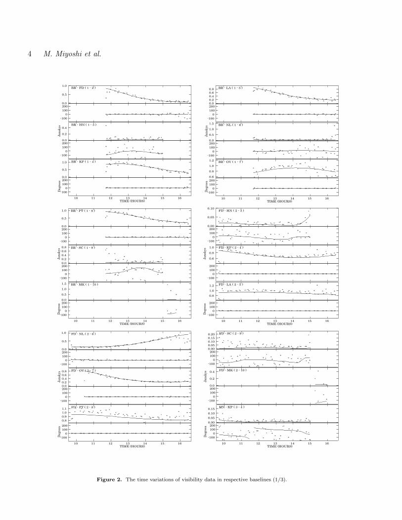
In order to make efficient use of as much data as pos-sible, we adopted a reduction strategy of keeping all datapoints till the final calibration stage where the CALIB (AIPStask of self-calibration) is performed. For data points whereno solution was obtained at FRING in AIPS, we assigneda value interpolated from adjacent good solutions to thedata points. Such keeping strategy in reduction is often per-formed for weaker maser data. We did the standard am-plitude calibrations using antenna gains in GC table andsystem temperatures in TY table with opacity correctionsin AIPS (NRAO). Further at the last stage of the data cal-ibrations we applied solutions of amplitude and phase fromthe task CALIB with an image model of the average size andshape of SgrA∗ at 43 GHz (single elliptical Gaussian withfull width at half maximum of 712µas×407µas, PA = 79.8◦,Bower et al. 2004) with 1 Jy in flux density. The applicationof the CALIB solutions to the data substantially reducedthe effect of atmospheric and instrumental variations on theobserved visibilities (Miyoshi et al. submitted to PASJ), andeffectively made visibilities of longer baselines available forimaging synthesis. Figure 1 shows that the u-v coverage ofthe solutions extends up to 5800 km (8.3×108λ) in projectedbaseline length. This will give us a spatial resolution of threetimes better than those of the previous studies (Bower et al.1998, 2004). We show the amplitude and phase variations ofthe calibrated visibilities of respective baselines and closurephases for all triangles in Figures 2, 3, & 4 and Figures 5,6, & 7 respectively.

2.1 The u-v coverage of the calibrated data

We got calibration solutions from 43 baselines out of all the45 baselines, though not during the whole observing time.While we found no solution from SC-MK and HN-MK base-lines. As for the baselines connected to MK, we found effec-tive visibilities when the projected baseline length becomesshorter than 5800 km during the last one-half hours of theobserving session. Except SC-MK and HN-MK, we found so-lutions from the 7 baselines (BR-MK, FD-MK, KP-MK, LA-MK, NL-MK, OV-MK, and PT-MK). As for the baselinesconnected to SC, we found solutions from the 8 baselines(BR-SC, FD-SC, HN-SC, KP-SC, LA-SC, NL-SC, OV-SC,and PT-SC). We found none of solution from the SC-MKbaseline. As for the baseline connected to HN, except thebaseline between MK we found solutions from the 8 base-lines (BR-HN, FD-HN, HN-KP, HN-LA, HN-NL, HN-OV,HN-PT, and HN-SC). As for the baselines connected to BR,

we found solutions from all the baselines. Though the BRstation locates at high latitude, we often find good visibili-ties of SgrA∗because the projected baseline length becomesshorter for the SgrA∗observations. The all of resultant u-v coverage distribute up to 8.3 × 108λ (5800 km) in radius(Figure 1).

2.2 Visibility variation in each baseline

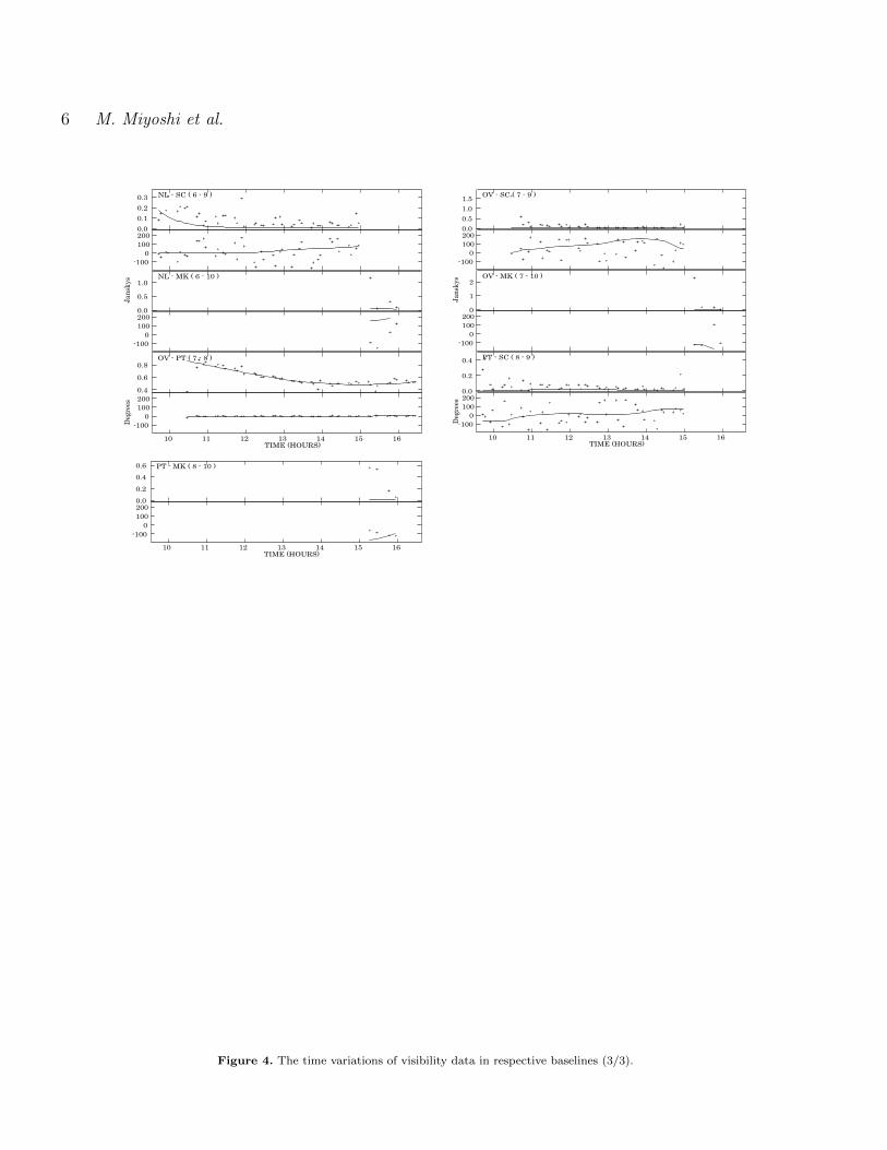
Figures 2, 3, & 4 show the time variations of the amplitudeand phase of each baseline (each point is 5 min integration).The lines in every plot show the time variations of the am-plitude and phase calculated from the obtained image fromthe whole time integration (Figure 8 a). From the compar-ison between the real visibilities and calculated ones fromthe image, we can classify them into 6 categories.

(i) The phase is constantly zero and the amplitude hasno variation with time. Namely the source SgrA∗is observedas an unresolved point source for the corresponding fringespacing of the baselines: 2 baselines, KP-PT and LA-PTshow this feature. The maximum projected baseline lengthsare about 400 km (KP-PT) and 210 km (LA-PT). The cor-responding fringe spacings are 3.5 mas and 6.7 mas respec-tively.

(ii) The calculated phases and amplitudes from the ob-tained image, and the real ones coincide each other well.The phases are constantly zero, while the amplitudes varywith projected baseline length. The observed source SgrA∗ispartially resolved by the spatial resolutions of the baselines.In other words, SgrA∗was observed to be not infinitely smallbut have a size: 19 baselines, namely BR-FD, BR-KP, BR-LA, BR-OV, BR-PT, FD-KP, FD-LA, FD-NL, FD-OV, FD-PT, HN-NL, HN-SC, KP-LA, KP-NL, KP-OV, LA-NL, LA-OV, NL-PT, & OV-PT, belong to this category. The aver-age of these maximum projected baseline lengths is about1400 km (1 mas in fringe spacing: from here in bracket afterprojected baseline length, we note the corresponding fringespacing), the shortest ones are about 560 km (2.5 mas) (FD-LA, FD-PT) and the longest one is about 2650 km (0.53mas) (HN-SC).

(iii) The calculated phases from the obtained image, andthe real ones coincide each other or show similarity. Whilethe amplitudes from both do not show similarity. 3 baselines,BR-SC, BR-MK, PT-MK, belong to this category. The max-imum projected baseline lengths are 5740 km (0.24 mas),3850 km (0.36 mas), and 4760 km (0.29 mas) respectively.

(iv) The calculated phases from the obtained image, andthe real ones do not coincide each other. While the am-plitudes from both show similarity and match in some de-gree: 12 baselines, BR-HN, BR-NL, FD-HN, HN-KP, HN-LA, HN-OV, HN-PT, KP-SC, NL-OV, HN-SC, OV-SC, &PT-SC, belong to this category. The average of these max-imum projected baseline lengths is about 3710 km (0.38mas), the shortest one is about 2380 km (0.59 mas) (NL-OV)and the longest one is about 5530 km (0.25 mas) (OV-SC).

(v) The calculated visibility and the real ones do not showmatching both in phase and in amplitude: 7 baselines, FD-SC, FD-MK, KP-MK, LA-SC, LA-MK, NL-MK, & OV-MK,belong to this category. In general there are at least threepossibilities to explain the no-matching. One is due to a lowsignal to noise ratio including the case of no signal. Another

c© 20** RAS, MNRAS 000, 1–??

Oscillation in SgrA∗ 3

Figure 1. The u-v coverage of all the visibility data that have calibration solutions by our reduction method.

is due to the complex structure of the real source, the ob-tained rough image could not reproduce the real visibilityvariations. The other is the mixture of the two cases above.The average of these maximum projected baseline lengths isabout 4650 km (0.30 mas), the shortest ones are about 3920km (0.36 mas) (NL-OV) and the longest one is about 5670km (0.25 mas) (OV-SC).

(vi) No solution is found in SC-MK and HN-MK base-lines, which are longer than 5800 km in projected baselinelength.

Assuming that matching between the observed and thecalculated visibilities mean sufficient calibrations of the twostations of the baseline, we can guess whether the calibra-tions both of the stations are good or bad. (Here we think

that mis-matching does not necessarily mean bad calibra-tions. If the observed visibility is from time variable sourcein structure, any single image cannot satisfy the whole timevisibility variation. However, if the structure variation is notso large one, such a small variation is negligible and not de-tectable for shorter baselines.) By eye, we found that thefollowing baselines seem in the matching: BR-FD, BR-KP,BR-LA, BR-OV, BR-PT, FD-KP, FD-LA, FD-NL, FD-OV,FD-PT, HN-NL, HN-SC, KP-NL, KP-OV, KP-PT, LA-NL,LA-OV, LA-PT, NL-PT, and OV-PT. If the assumption iscorrect, except the MK station, other 9 stations seem to bewell-calibrated anyway.

c© 20** RAS, MNRAS 000, 1–??

4 M. Miyoshi et al.

1.0

0.5

0.0

BR - FD ( 1 - 2 )

200100

0-100

Jans

kys 0.4

0.2

0.0

BR - HN ( 1 - 3 )

200100

0-100

1.0

0.5

0.0

BR - KP ( 1 - 4 )

Degr

ees

TIME (HOURS)10 11 12 13 14 15 16

200100

0-100

0.80.60.40.20.0

BR - LA ( 1 - 5 )

200100

0-100

Jans

kys 1.5

1.00.50.0

BR - NL ( 1 - 6 )

200100

0-1001.21.00.80.6

BR - OV ( 1 - 7 )

Degr

ees

TIME (HOURS)10 11 12 13 14 15 16

200100

0-100

1.0

0.5

0.0

BR - PT ( 1 - 8 )

200100

0-100

Jans

kys 0.8

0.60.40.20.0

BR - SC ( 1 - 9 )

200100

0-1001.51.00.50.0

BR - MK ( 1 - 10 )

Degr

ees

TIME (HOURS)10 11 12 13 14 15 16

200100

0-100

0.10

0.05

0.00

FD - HN ( 2 - 3 )

200100

0-100

Jans

kys 1.0

0.80.6

FD - KP ( 2 - 4 )

200100

0-100

1.21.00.8

FD - LA ( 2 - 5 )

Degr

ees

TIME (HOURS)10 11 12 13 14 15 16

200100

0-100

1.0

0.5

0.0

FD - NL ( 2 - 6 )

200100

0-100

Jans

kys 0.8

0.60.40.20.0

FD - OV ( 2 - 7 )

200100

0-100

1.11.00.90.8

FD - PT ( 2 - 8 )

Degr

ees

TIME (HOURS)10 11 12 13 14 15 16

200100

0-100

0.200.150.100.050.00

FD - SC ( 2 - 9 )

200100

0-100

Jans

kys 0.4

0.2

0.0

FD - MK ( 2 - 10 )

200100

0-100

0.150.100.050.00

HN - KP ( 3 - 4 )

Degr

ees

TIME (HOURS)10 11 12 13 14 15 16

200100

0-100

Figure 2. The time variations of visibility data in respective baselines (1/3).

c© 20** RAS, MNRAS 000, 1–??

Oscillation in SgrA∗ 5

0.10

0.05

0.00

HN - LA ( 3 - 5 )

200100

0-100

Jans

kys

0.40.30.20.10.0

HN - NL ( 3 - 6 )

200100

0-100

0.200.150.100.050.00

HN - OV ( 3 - 7 )

Degr

ees

TIME (HOURS)10 11 12 13 14 15 16

200100

0-100

0.150.100.050.00

HN - PT ( 3 - 8 )

200100

0-100

Jans

kys 0.8

0.60.40.20.0

HN - SC ( 3 - 9 )

200100

0-1001.21.00.80.6

KP - LA ( 4 - 5 )

Degr

ees

TIME (HOURS)10 11 12 13 14 15 16

200100

0-100

0.4

0.2

0.0

KP - NL ( 4 - 6 )

200100

0-100

Jans

kys 1.0

0.5

0.0

KP - OV ( 4 - 7 )

200100

0-100

1.0

0.5

0.0

KP - PT ( 4 - 8 )

Degr

ees

TIME (HOURS)10 11 12 13 14 15 16

200100

0-100

1.0

0.5

0.0

KP - SC ( 4 - 9 )

200100

0-100

Jans

kys 1.5

1.00.50.0

KP - MK ( 4 - 10 )

200100

0-100

0.80.60.40.20.0

LA - NL ( 5 - 6 )

Degr

ees

TIME (HOURS)10 11 12 13 14 15 16

200100

0-100

0.80.70.60.50.4

LA - OV ( 5 - 7 )

200100

0-100

Jans

kys 1.2

1.00.80.6

LA - PT ( 5 - 8 )

200100

0-100

0.30.20.10.0

LA - SC ( 5 - 9 )

Degr

ees

TIME (HOURS)10 11 12 13 14 15 16

200100

0-100

1.0

0.5

0.0

LA - MK ( 5 - 10 )

200100

0-100

Jans

kys 0.4

0.30.20.10.0

NL - OV ( 6 - 7 )

200100

0-100

0.60.40.20.0

NL - PT ( 6 - 8 )

Degr

ees

TIME (HOURS)10 11 12 13 14 15 16

200100

0-100

Figure 3. The time variations of visibility data in respective baselines (2/3).

c© 20** RAS, MNRAS 000, 1–??

6 M. Miyoshi et al.

0.30.20.10.0

NL - SC ( 6 - 9 )

200100

0-100

Jans

kys 1.0

0.5

0.0

NL - MK ( 6 - 10 )

200100

0-100

0.80.60.4

OV - PT ( 7 - 8 )

Degr

ees

TIME (HOURS)10 11 12 13 14 15 16

200100

0-100

1.51.00.50.0

OV - SC ( 7 - 9 )

200100

0-100

Jans

kys 2

1

0

OV - MK ( 7 - 10 )

200100

0-100

0.4

0.2

0.0

PT - SC ( 8 - 9 )

Degr

ees

TIME (HOURS)10 11 12 13 14 15 16

200100

0-100

0.60.40.20.0

PT - MK ( 8 - 10 )

TIME (HOURS)10 11 12 13 14 15 16

200100

0-100

Figure 4. The time variations of visibility data in respective baselines (3/3).

c© 20** RAS, MNRAS 000, 1–??

Oscillation in SgrA∗ 7

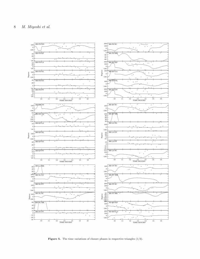
2.3 Closure phases

Figures 5, 6, & 7 show the time variations of the closurephases of all triangles composed from three stations. Everypoint is from 15 min integration. We also calculated theclosure phase variations from the images of the whole timeintegration as shown in Figure 8 (a). Closure phases showseveral features as below.

(i) First feature is seen in the small triangles composedfrom inner stations of the VLBA, namely FD, LA, PT, KP,& OV. The projected extensions of the triangles range from700 km (2 mas) to 1600 km (0.88 mas), and the averageis 1200 km (1.2 mas). These 10 triangles show nearly zeroconstant closure phases, a few degree variations at most.This indicates that SgrA∗is observed as a structure of pointsymmetric with the corresponding fringe spacings (0.88 −2mas).

(ii) Second feature is seen in the 10 triangles composedfrom BR and other two stations from the inner 5 stations,FD, LA, PT, KP, & OV. The projected extensions of thetriangles range from 1500 km (0.93 mas) to 2200 km (0.64mas), and the average is 1900 km (0.74 mas). The closurephases show zero on average, but fluctuating ±40◦ at peak.

(iii) Third feature is seen in the 10 triangles composedfrom NL and other two stations from the inner 5 stations,FD, LA, PT, KP, & OV. The projected extensions of thetriangles range from 1800 km (0.78 mas) to 2800 km (0.5mas), and the average is 2400 km (0.58 mas). The closurephases show zero on average, but fluctuating by ±60◦ onaverage, ±100◦ at maximum case.

(iv) In most of large triangles which have projected exten-sions up to 5800 km (0.24 mas), the closure phases distribute±180◦. However, some of triangles including MK stationshow nearly constant and/or very small variations in closurephase though the duration is about 40 minutes. Two triangleof FD-NL-MK and LA-PT-MK show closure phase variationwithin 15◦, triangle of KP-PT-MK shows that within 10◦,and triangle of KP-LA-MK shows nearly constant closurephase within 8◦ variation. The projected extensions of thesethree cases range from 4800 km (0.29 mas) to 5200 km (0.27mas), 4900 km (0.29 mas) respectively.

(v) In most of the large triangles, the real closure phaseand the calculated phase from the obtained image do notmatch. While one of the large triangles, HN-NL-OV showsmatching between them. The projected extension of the tri-angles is about 4200 km (0.33mas).

(vi) The last feature is seen in the five of triangles BR-FD-KP, BR-FD-LA, BR-FD-NL, BR-FD-OV, BR-FD-PT,whose projected extensions range from 2100 (0.67 mas) kmto 2500 km (0.56 mas), and the average is 2300 km (0.64mas). They show very similar closure phase variations eachother.

2.4 The calibrations of MK, SC, and HN stations

Visibility plots (Figure 2,3, and 4) and closure plots (Figure5,6, and 7) show that the SC and HN stations are calibrated,though not perfect. The visibility plots of HN-NL, and HN-SC shows quite a good match between the real amplitudes &phases and the calculated ones from the obtained map. Thevisibility plot of BR-SC shows good match in phase varia-tion, that of FD-HN shows good match in amplitude vari-

ation. Presumably, the HN and SC stations are calibratedquite well. At least, the calibrations to the HN and SC sta-tions remove largely the systematic errors.About the MK station, the calibration solutions were ob-tained for the last one hour. Because the duration is short,the match in visibility is difficult to confirm. But, some ofthe triangles including MK station show nearly constantand/or very small variations in closure phase. These featurespresumably mean that the MK station got fringes betweenother stations though the signals are weak.In APPENDIX D, we show several images by omitting thevisibility data of the baselines to the MK, SC, HN stations.These images suggest that the calibration errors and thelow SNR of the data from three stations have little influ-ence upon the image quality.

2.5 Obtained image from the whole time dataintegration

We made an image from the whole time integration usingthe task IMAGR in AIPS with loop gain parameters (GAIN)= 0.005, limit of subtracting iterations (NITER) = 20000,maximum residual flux density level (FLUX) = 0.005 Jy,and u-v Gaussian tapering (UVTAPER) = 6000 km. Herewe used the wider tapering in u-v with expectations of beingable to use lower SNR data points by the CALIB solutions.The mapping area is 3 mas (e−w)× 6 mas (n− s) and theboxing area is 2.13 mas (e − w) × 4.17 mas (n − s) at thecenter. Because the sizes of SgrA∗at 43GHz are well known,we limited the peak search to the central area to avoid se-lecting side lobe area. The grid numbers are 1024 (e−w)×2048 (n− s), namely the grid spacing is nearly 2.93µas. Byusing a smaller grid, we intended to select the peak positionsas accurately as possible. We performed the imaging with arestoring beam of 0.40 mas× 0.15 mas, PA = 0◦

The obtained image from the whole time integration sug-gests that the calibration of the visibilities are success-fully performed. From direct fitting of an elliptical Gaussianshape to the image and the deconvolution of the restoringbeam shape, we got a result of the shape and size. The ma-jor axis is 0.759+0.006

−0.007 mas, the minor axis is 0.323 ± 0.007mas, and the position angle is PA = 85.1± 1◦. This estima-tion is consistent to the previous measurement of the samedata using closure amplitude by Shen et al. (2005) that showthe major axis is 0.722 ± 0.002 mas, and the minor axis is0.395+0.019

−0.020 mas and the PA is 80.4 ± 0.8 ◦. The deviationsfrom the Shen’s measurement are +0.037 mas in major axis,−0.072 mas in minor axis and 4.6◦ in PA. Miyoshi et al. (sub-mitted to PASJ) show the details of the results from otherVLBA data on SgrA∗at 43GHz with the same reductionmanner. The consistent Gaussian shape and size to thosefound Shen et al. (2005) indicates that we got better cali-bration solutions from the CALIB and that we successfullyobtained images of SgrA∗with better spatial resolution thanbefore.

3 ANALYZING METHOD AND RESULTS

We investigated the spatial distributions of oscillations influx density with two independent methods. The first one is

c© 20** RAS, MNRAS 000, 1–??

8 M. Miyoshi et al.

200100

0-100

BR-FD-SC

0-20-40-60

BR-FD-MK

200100

0-100

BR-HN-KP

Degr

ees 100

0

-100

BR-HN-LA

1000

-100

BR-HN-NL

TIME (HOURS)10 11 12 13 14 15 16

200100

0-100

BR-HN-OV

1000

-100

BR-FD-HN

40200

-20

BR-FD-KP

40200

-20

BR-FD-LA

Degr

ees 100

0-100

BR-FD-NL

40200

-20

BR-FD-OV

TIME (HOURS)10 11 12 13 14 15 16

20100

-10-20

BR-FD-PT

1000

-100

BR-HN-PT

500

-50-100-150

BR-HN-SC

100

-10

BR-KP-LA

Degr

ees 100

0-100

BR-KP-NL

4020

0

BR-KP-OV

TIME (HOURS)10 11 12 13 14 15 16

20100

-10-20

BR-KP-PT

1000

-100

BR-KP-SC

10080604020

BR-KP-MK

1000

-100

BR-LA-NL

Degr

ees 30

20100

-10

BR-LA-OV

100

-10-20

BR-LA-PT

TIME (HOURS)10 11 12 13 14 15 16

200100

0-100

BR-LA-SC

6040200

BR-LA-MK

200100

0-100

BR-NL-OV

1000

-100

BR-NL-PT

Degr

ees 100

0-100

BR-NL-SC

60

40

20

BR-NL-MK

TIME (HOURS)10 11 12 13 14 15 16

100

-10-20-30

BR-OV-PT

1000

-100

BR-OV-SC

100500

-50

BR-OV-MK

200100

0-100

BR-PT-SC

Degr

ees -40

-60-80

-100-120-140

BR-PT-MK

200100

0-100

FD-HN-KP

TIME (HOURS)10 11 12 13 14 15 16

200100

0-100

FD-HN-LA

Figure 5. The time variations of closure phases in respective triangles (1/3).

c© 20** RAS, MNRAS 000, 1–??

Oscillation in SgrA∗ 9

1000

-100

FD-HN-NL

1000

-100

FD-HN-OV

200100

0-100

FD-HN-PT

Degr

ees 200

1000

-100

FD-HN-SC

6420

-2-4

FD-KP-LA

TIME (HOURS)10 11 12 13 14 15 16

500

-50

FD-KP-NL

0

-10

-20

FD-KP-OV

3020100

FD-KP-PT

200100

0-100

FD-KP-SC

Degr

ees 0

-50-100-150

FD-KP-MK

40200

FD-LA-NL

TIME (HOURS)10 11 12 13 14 15 16

0-20-40-60

FD-LA-OV

20

100

FD-LA-PT

1000

-100

FD-LA-SC

150100500

FD-LA-MK

Degr

ees 100

0-100

FD-NL-OV

40

20

0

FD-NL-PT

TIME (HOURS)10 11 12 13 14 15 16

1000

-100

FD-NL-SC

2015105

FD-NL-MK

50

-5-10

FD-OV-PT

1000

-100

FD-OV-SC

Degr

ees

806040200

FD-OV-MK

200100

0-100

FD-PT-SC

TIME (HOURS)10 11 12 13 14 15 16

500

-50-100-150

FD-PT-MK

200100

0-100

HN-KP-LA

200100

0-100

HN-KP-NL

200100

0-100

HN-KP-OV

Deg

rees

200100

0-100

HN-KP-PT

1000

-100

HN-KP-SC

TIME (HOURS)10 11 12 13 14 15 16

200100

0-100

HN-LA-NL

1000

-100

HN-LA-OV

200100

0-100

HN-LA-PT

200100

0-100

HN-LA-SC

Deg

rees 100

0-100

HN-NL-OV

200100

0-100

HN-NL-PT

TIME (HOURS)10 11 12 13 14 15 16

200100

0-100

HN-NL-SC

Figure 6. The time variations of closure phases in respective triangles (2/3).

c© 20** RAS, MNRAS 000, 1–??

10 M. Miyoshi et al.

200100

0-100

HN-OV-PT

200100

0-100

HN-OV-SC

200100

0-100

HN-PT-SC

Degr

ees 50

0

-50

KP-LA-NL

0

-20

-40

KP-LA-OV

TIME (HOURS)10 11 12 13 14 15 16

420

-2

KP-LA-PT

1000

-100

KP-LA-SC

-18-20-22-24-26

KP-LA-MK

200100

0-100

KP-NL-OV

Degr

ees 50

0

-50

KP-NL-PT

200100

0-100

KP-NL-SC

TIME (HOURS)10 11 12 13 14 15 16

0-50

-100-150

KP-NL-MK

0-10-20-30

KP-OV-PT

200100

0-100

KP-OV-SC

16014012010080

KP-OV-MK

Degr

ees

200100

0-100

KP-PT-SC

-150

-155

-160

KP-PT-MK

TIME (HOURS)10 11 12 13 14 15 16

200100

0-100

LA-NL-OV

20100

-10

LA-NL-PT

200100

0-100

LA-NL-SC

0-50

-100-150

LA-NL-MK

Degr

ees 0

-20-40-60-80

LA-OV-PT

200100

0-100

LA-OV-SC

TIME (HOURS)10 11 12 13 14 15 16

100

0

-100

LA-OV-MK

200

100

0

LA-PT-SC

-125-130-135-140

LA-PT-MK

200100

0-100

NL-OV-PT

Degr

ees 200

1000

-100

NL-OV-SC

6040200

NL-OV-MK

TIME (HOURS)10 11 12 13 14 15 16

200100

0-100

NL-PT-SC

0-50

-100-150

NL-PT-MK

200100

0-100

OV-PT-SC

1401201008060

OV-PT-MK

TIME (HOURS)10 11 12 13 14 15 16

Degr

ees

Figure 7. The time variations of closure phases in respective triangles (3/3).

c© 20** RAS, MNRAS 000, 1–??

Oscillation in SgrA∗ 11

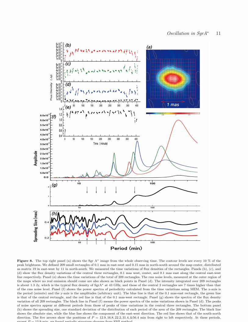
Figure 8. The top right panel (a) shows the Sgr A∗ image from the whole observing time. The contour levels are every 10 % of thepeak brightness. We defined 209 small rectangles of 0.1 mas in east-west and 0.15 mas in north-south around the map center, distributed

as matrix 19 in east-west by 11 in north-south. We measured the time variations of flux densities of the rectangles. Panels (b), (c), and(d) show the flux density variations of the central three rectangles, 0.1 mas west, center, and 0.1 mas east along the central east-west

line respectively. Panel (e) shows the time variations of the total of 209 rectangles. The rms noise levels, measured at the outer region of

the maps where no real emission should come are also shown as black points in Panel (d). The intensity integrated over 209 rectanglesis about 1.3 Jy, which is the typical flux density of SgrA∗ at 43 GHz, and those of the central 3 rectangles are 7 times higher than that

of the rms noise level. Panel (f) shows the power spectra of periodicity calculated from the time variations using MEM. The x-axis isthe period (minute) and the y-axis is the amplitudes (arbitrary unit). The blue line is that of the 0.1 mas-east rectangle, the green line

is that of the central rectangle, and the red line is that of the 0.1 mas-west rectangle. Panel (g) shows the spectra of the flux density

variation of all 209 rectangles. The black line in Panel (f) means the power spectra of the noise variations shown in Panel (d). The peaksof noise spectra appear at different periods from those of peaks of time variations in the central three rectangles. The bottom panel

(h) shows the spreading size, one standard deviation of the distribution of each period of the area of the 209 rectangles. The black line

shows the absolute size, while the blue line shows the component of the east-west direction. The red line shows that of the south-northdirection. The five arrows show the positions of P = 12.9, 16.8, 22.2, 31.4,&56.4 min from right to left respectively. At these periods,

except P = 12.9 min, we found periodic structure changes from SMI method.c© 20** RAS, MNRAS 000, 1–??

12 M. Miyoshi et al.

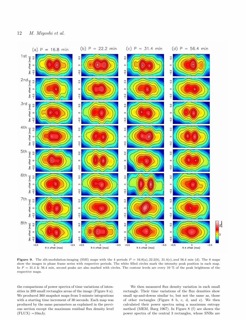
Figure 9. The slit-modulation-imaging (SMI) maps with the 4 periods P = 16.8(a), 22.2(b), 31.4(c), and 56.4 min (d). The 8 mapsshow the images in phase frame series with respective periods. The white filled circles mark the intensity peak position in each map.

In P = 31.4 & 56.4 min, second peaks are also marked with circles. The contour levels are every 10 % of the peak brightness of therespective maps.

the comparisons of power spectra of time variations of inten-sities in 209 small rectangles areas of the image (Figure 8 a).We produced 360 snapshot maps from 5-minute integrationswith a starting time increment of 30 seconds. Each map wasproduced by the same parameters as explained in the previ-ous section except the maximum residual flux density level(FLUX) =10mJy.

We then measured flux density variation in each smallrectangle. Their time variations of the flux densities showsmall up-and-downs similar to, but not the same as, thoseof other rectangles (Figure 8 b, c, d, and e). We thencalculated their power spectra using a maximum entropymethod (MEM, Burg 1967). In Figure 8 (f) are shown thepower spectra of the central 3 rectangles, whose SNRs are

c© 20** RAS, MNRAS 000, 1–??

Oscillation in SgrA∗ 13

more than 7, while in Figure 8 (g) are the spectra of time-variations of all 209 rectangles shown in Figure 8 (e).

Figure 8 (h) shows the spreading size σ(P ), namely theone standard deviation of the spatial distribution of the am-plitude of each period. The definition is

σ(P ) = sqrt[

209∑i=1

(x2i + y2i ) ·Ai(P )/S(P )] (1)

The component in x direction is

σx(P ) = sqrt[

209∑i=1

x2i ·Ai(P )/S(P )] (2)

The component in y direction is

σy(P ) = sqrt[

209∑i=1

y2i ·Ai(P )/S(P )] (3)

,where S(P ) =∑209

i=1Ai(P ), the sum of the amplitudes

in the 209 rectangles. The i means ith rectangle, P is theperiod, Ai(P ) is the amplitude of the period in each rect-angle, (xi, yi) is the central position of the ith rectangle.If all of the power of the period concentrate at the centralrectangle i = 0, the spreading sizes σ(P ), σx(P ), & σx(P )are zero. If the power distributes uniformly in all the rectan-gles, the spreading sizes are 0.362 mas in σ(P ), 0.274 mas inσx(P ), and 0.237 mas in σx(P ). In the case that the spread-ing sizes are larger than these values, the power of the periodmainly comes from outer area, where the flux density andthe SNRs are lower. Such periods with larger spreading sizespresumably originate from noise. If the spreading sizes of theperiods are smaller than these values, the power of the pe-riods comes from the central part of the image, where theflux density and the SNR is higher. A real periodicity, if de-tected, because it should come from the central part of theimage, the spreading size should be smaller than that of theuniform case.

Small spreading sizes, or the concentrations of thedistributions at the center, are seen around P =12.9, 17.2, 30.1, and 55.8 min, where the amplitude shows amaximum (Figure 8 g). Loose concentrations appear aroundP = 128.4, and 268 min though they are under-sampled.

The first method tends to be affected by differences of u-v sampling between snap shot maps. We hence devised andused a new method, slit-modulation-imaging (SMI) whichis a way of examining the existence of the periodic struc-tural change with an assuming period and almost free fromu-v sampling differences (Miyoshi, 2008). SMI maps are ob-tained as follows: we divided the whole observation time intoseveral sections with the trial period P min interval and theneach section was sub-divided into 8 phase-segments. Thefirst-phase SMI map was produced with visibilities from thefirst phase-segments of all the sections. The second-phaseSMI map was produced with visibilities from the secondphase-segments of all the sections. Namely, the n-th phaseSMI map is produced from the visibilities of the n-th phase-segments of all the sections. Thus, the SMI maps have u-v coverage very similar to each other, and are almostfree from the effect of differing u-v coverages (Figure 10).Characteristic structure changes with the period will be en-hanced and emerge onto the respective SMI maps if it ex-ists. (Miyoshi 2008)

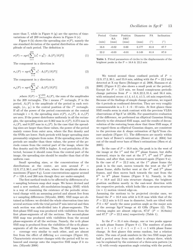
Period Center Position Diameter PA Inclination

RA DEC

(min) (mas) (mas) (mas) (◦) (◦)

16.8 -0.02 0.00 0.177 81.8 87.7

22.2 -0.03 -0.01 0.149 81.8 87.0

Table 1. Fitted parameters of circles to the displacements of thebrightest peaks in the P = 16.8 & 22.2 min

We tested around these confined periods of P =12.9, 17.2, 30.1, and 55.8 min, adding with the P = 22.2 mindetected at X ray flares (Belanger et al. 2006, Hamaus et al.2009) (Figure 8 (f) also shows a small peak at the period).Except for P = 12.9 min, we found conspicuous periodicchange patterns from P = 16.8, 22.2, 31.4, and 56.4 min,with estimated errors ±1.4,±1.4,±1.5,±6 min respectively.Because of the findings of simple change patterns, we regardthe 4 periods as confirmed detection. They are very roughlycommensurable in a 3 : 4 : 6 : 10 ratio. At first glance theseSMI results seem in stark contrast with the previous VLBAobservations of SgrA∗at 43GHz. For quantitative evaluationof the difference, we performed an elliptical Gaussian fittingdirectly to the obtained SMI maps, and the results of decon-volution of the restoring beam show that these SMI maps, ifwe regard them as elliptical Gaussian shapes, are consistentto the previous size & shape estimation of SgrA∗from clo-sure analysis (Figure 11). The differences are mostly withinerror bars of Bower’s estimations (Bower et al. 2004) butout of the small error bars of Shen’s estimations (Shen et al.2005)

In the case of P = 16.8 min, the peak is in the west ofthe image at the 1st and the 2nd phase frames, but shiftseastward, stays in the east at the 3rd, 4th and 5th phaseframes, and after that, moves westward again (Figure 9 a).In the case of P = 22.2 min, at the 1st phase frame thepeak is in the east, moves towards the west at the 2nd

phase frame, shifts further west at the 4th and 5th phaseframes, and then moves back towards the east from the6th to 8th phase frames (Figure 9 b). Namely, in theP = 16.8 and 22.2 min structure changes, the brightestposition oscillates mostly in the east-west direction withthe respective periods, which looks like a one-arm structure(m = 1) motion viewed edge-on.Assuming the motions to be projected circular ones, wefound the P = 16.8 min orbit is 0.18 mas while that of theP = 22.2 min is 0.15 mas in diameter, both are tilted withPA = 82◦ nearly the same position angle as the major axisof the average SgrA∗image at 43 GHz (Figure 12). Theviewing angles are almost edge-on, 87.0◦ (P = 16.8min)and 87.7◦ (P = 22.2 min) respectively (Table 1).

In the P = 31.4 min change, one or two peaks appearin each phase frames (Figure 9 c). The numbers of peaksare 2 → 1 → 2 → 2 → 1 → 2 → 1 → 1 with phase framechange. At first glance this seems random, but a relationexists. The sum of peak numbers in the two SMI maps justhalf a period away from each other is always three, whichcan be explained by the existence of a three-arm pattern (m= 3) with evenly separation angle rotating with the period,

c© 20** RAS, MNRAS 000, 1–??

14 M. Miyoshi et al.

Figure 10. The u-v coverage of the respective SMI maps.

c© 20** RAS, MNRAS 000, 1–??

Oscillation in SgrA∗ 15

Figure 11. Gaussian size estimations of the each SMI maps. The dashed line shows the parameter obtained from the whole time

integration image. The dot line shows the parameters estimated from closure analysis (Shen et al. 2005).

which we view edge-on.

In the P = 56.4 min change, one peak appears duringa half period (the 6th to 8th, and 1st phase frames) and twopeaks appear during the last half period from the 2nd to the5th phase frame (Figure 9 d). This is due to the amplitude ofvariation at the central 50 µas being twice as large as thoseof the surroundings. One peak appears when the central partbecomes bright, and two peaks, one on the east and one onthe west, appear when the central part darkens. Unlike otherperiods, the P = 56.4 min component seems concentratedand excited at the radius close to the black hole where therelativistic effect are not negligible, and hence it can be akey to distinguishing the origin of QPOs.

The detected pattern changes are not from noise ef-fects: we simulated changes using artificial visibilities withnoise levels showing the comparable amplitude fluctuationswith those of real visibility data. SMI images from the arti-ficial visibilities show larger variations in not east-west butsouth-north direction that the spatial resolution is worse,

while those from the observations show the opposite ten-dency. From the artificial visibilities, changes appeared inthe image but none of the periodic regular patterns couldbe found. Also the artificial visibilities showed no coincidentoccurrence between spreading size minima and amplitudepeaks in the spectra of the whole 209 area. Further, the ob-served periodic changes of real data basically did not disap-pear in SMI-maps with shorter total integration times (195min) while different changes appeared from the artificial vis-ibilities.

4 DISCUSSION AND CONCLUSION

The radio QPOs reported here have a delay of 1.5 days fromthe millimeter wave flare, and the distributions extended to100 Rs in apparent diameter while the QPOs in NIR andX ray are just at the flaring time and estimated to occuraround a marginally stable orbit (MSO) (Genzel et al. 2003;Aschenbach et al. 2004; Eckart et al. 2006 and Belanger et al.

c© 20** RAS, MNRAS 000, 1–??

16 M. Miyoshi et al.

Figure 12. The offset of brightness peak positions in the frame series of SMI images: those of P= 16.8 min in the left panels and those

of P= 22.2 min in the right panels. The top panels show the positional shifts in R.A. while the middle panels in declination. The curvein each panel shows the sinusoidal function obtained from fitting to the data. The bottom panels show the displacements of the peaks in

the sky. The ellipses are formed from the obtained fitted sine curves.

2006). The flaring events at MSO would vibrate the wholesystem to excite fundamental disk oscillation modes, whichwould last for several days at least.

There are features that cannot be explained as Keple-rian motions directly governed by centripetal force, but thatare easily interpretable as disk oscillation features (Kato etal. 2008). First, the counter-rotations occurred simultane-ously between the P = 16.8 min and P = 22.2 min periods,which is difficult to be explained by a single body motionlike hot spot models. Second, the orbit of the shorter periodP = 16.8 min is larger than that of the P = 22.2min, whichcannot be realized by a Keplerian motion.

If QPOs originate in a strong gravity field where therelativistic effect plays an important role, the periods ofQPOs should depend on the mass and the spin of a massiveblack hole. Recent theories of disk seismology (Kato etal. 2008; Abramowicz et al. 2001) predict that peak fre-quencies of QPOs can be scaled by a mass of central black

holes as an analogy to QPOs in black hole x-ray binaries(BXB) (Remillard, & McClintock 2006). For example, inGRO J1655-40, a peak frequency of high frequency QPOs isabout 3× 102(6.0− 6.6M�/MBH) Hz (where M� is a solarmass), with the result that a corresponding peak frequencyusing the mass of SgrA∗derived from the orbital motions ofsurrounding stars (3.6 ± 0.3 × 106M�) (Eisenhauer et al.2005) is about 5.1 × 10−4 Hz (P = 32min), which is one ofour findings. Detailed analysis with the obtained four QPOperiods and wave-warp resonant oscillation model predictsthe spin of SgrA∗to be 0.44± 0.08 and the black hole massto be (4.2± 0.4)× 106M�. (Kato et al. submitted to MN)

The apparent angular size of 0.1 mas corresponds to10.4Rs(1Rs is Schwarzschild radius) assuming the Galacticcenter distance to be 7.6 kpc. (Eisenhauer et al. 2005),which scale give us that the orbital velocities of brightpeak positions are vP=16.8min = 2.1 c at 8.8 Rs and

c© 20** RAS, MNRAS 000, 1–??

Oscillation in SgrA∗ 17

vP=22.2min = 1.4 c at 7.4 Rs, both are superluminal,but can be explained as follows. It is well-known thatthe VLBI images of SgrA∗ are obscured and broadenedby the scatterings of surrounding plasma (Lo et al. 1998;Doeleman et al. 2001). If we consider the broadeningratio of 2.6 ∼ 3.0 at 43 GHz by scattering (Shen etal. 2005; Bower et al. 2004), and the magnifying ratio∼ 1.23 by self-gravitational lensing effect at 3 Rs , theapparent 0.1 mas observed at 43 GHz is equal to 2.8 to3.3 Rs in the intrinsic image of SgrA∗. Taking into theseeffects, we find that v′P=16.8min = 0.43 c at 2.7 Rs andv′P=22.2min = 0.68 c at 2.3 Rs, which velocities arecomparable to the Keplerian velocities at r = 2− 4Rs froma black hole.

Presumably the emission region of our observed radioQPOs is different from those of other wavelength, eventhough the origin of oscillations is common. Kato et al.(2009) show that synthetic images of radio, NIR, and X-rayare quantitatively different, by using multi-wavelengthradiative transfer calculations including compton scatteringprocess in three-dimensional magnetized hot accretionflows. Without synchrotron self-compton (SSC) process,Takahashi et al. (2009) show that temporal fluctuation offlux density at shorter wavelength, where the disk becomesoptically thin, is insensitive to the non-axisymmetric diskstructure. A possible emission mechanism of NIR and X-raywavelengths in order for having common oscillations atradio wavelength is the SSC, which is dominant when massaccretion rate becomes large [see Fig. 4 (a) and (d) in Katoet al. 2009].

The amplitude of the QPOs were 22 mJy (P =16.8min), 24mJy (P = 22.2 min), 25mJy (P = 31.4min),and 20 mJy (P = 56.4 min) respectively, the total reached 90mJy, nearly 10 % of the constant flux density component ofthe image (= 980 mJy). The relative intensities of their pe-riods are about 2 or 3% level of the total flux density, whichis comparable ratio to those of X ray QPOs (5−10% level incase of X ray Low Frequency QPO, 1% level in case of X rayHigh Frequency QPO). Such structural changes will causefluctuations in fringe phase, rate and amplitude. Existenceof oscillations with periods shorter than the whole observ-ing time will be one of the reasons why the VLBI imagingof SgrA∗ is difficult so far. However at the same time, thedetection of these periodic pattern changes means the ob-scured radio image of SgrA∗ still bears the imprint of theintrinsic figure. The VLBA observations of SgrA∗, togetherwith oscillation analysis, will provide us a unique chance toinvestigate the strong gravity field around the massive blackhole SgrA∗ with order of Rsresolutions.

ACKNOWLEDGMENTS

We would like to thank Shoji Kato, Ryoji Matsumoto, ShinMineshige, Shinya Nitta, Mami Machida, Takahiro Kudoh,& Hitoshi Negoro for discussions about disk oscillations, andYoshiaki Tamura K. Y. Lo and James Moran for discussionabout period analysis. The Very Long Baseline Array is op-erated by the National Radio Astronomy Observatory, which

is a facility of the National Science Foundation, operated un-der cooperative agreement by Associated Universities Inc.

REFERENCES

Abramowicz, M. A., & Kluzniak, W., 2001, A&A, 374, L19Aschenbach, B., et al. 2004, A&A, 417, 71Baganoff, F. K., et al. 2001, Nature, 413, 45Belanger, G., et al. 2006, eprint arXiv:astro-ph/0604337Journal of Physics: Conference Series, Volume 54, 420

Bower, G. C.& Backer, D. C., 1998, ApJ, 496,L97Bower, G. C.; Falcke, H.; Backer, D. C.; Wright, M., 1999,in”The Central Parsecs of the Galaxy”, ASP ConferenceSeries, 186, 80.

Bower, G. C., et al. 2004, Science, 304, 704Broderick, A. E., & Loeb, A., 2005, MNRAS, 363, 353Broderick, A. E., & Loeb, A., 2006, ApJ, 636, L109Broderick, A. E., & Loeb, A., 2006, MNRAS, 367, 905Burg, J. P., 1967, paper presented at the 37th Annual In-ternational Meeting, Soc. of Explor. Geophys., OklahamaCity, Okla., Oct. 31

Doeleman, S. S., et al. 2001, AJ, 121, 2610Doeleman, S. S., et al. 2008, Nature, 455, 78Eckart, A., et al. 2006, A&A, 455, 1Eisenhauer, F., et al. 2005, ApJ, 628, 246Fabian, A. C.,et al.2009, Nature, 459, 540Falcke, H., Melia, F., & Agol, E., 2000, ApJ, 528, L13Genzel, R., et al. 2003, Nature, 425, 934Ghez, A. M., et al. 2000, Nature, 407, 349Hamaus, N., et al. 2009, ApJ, 692, 902Harms, R. J., et al. 1994, ApJ, 435, L35Kato, S., Fukue, J., & Mineshige, S., 2008, Kyoto Univer-sity Press, (2008)

Kato, Y., et al. 2009, MNRAS, 400, 1742Kato, Y., et al. submitted to MNRAS Letter.Lo, K. Y., et al. 1998, ApJ, 508, L61Meyer, L., et al. 2008, ApJ, 688, L17Miyazaki, A., et al. 2006, Journal of Physics: ConferenceSeries, Volume 54, Issue 1, pp. 363

Miyoshi, M., et al. 1995, Nature, 373, 127Miyoshi, M., et al. 2004, Prog. Theor. Phys., 155,186Miyoshi, M., et al. 2007, Publ. National Astron. Obs.Japan, 10, 15

Miyoshi, M., 2008, PASJ, 60, 1371Miyoshi, M., et al. submitted to PASJRemillard, R. A. & McClintock, J. E., 2006, ARA&A, 44,49

Schodel, R., et al. 2002, Nature, 419, 694Shen, Z.-Q., et al. 2005, Nature, 438, 62Takahashi, R., 2004, ApJ, 611, 996Takahashi, R., 2009, at GC work shopTanaka, Y., et al. 1995, Nature, 375, 659Yusef-Zadeh, F., et al. 2006, ApJ, 644, 198

APPENDIX A: THE SMI RESULTS AROUND P= 12.9 MIN

We here show the none detection cases of conspicuous pat-tern change with the trial periods using the SMI method.As shown in Figure 8 (f), (g), there is a small peak at the

c© 20** RAS, MNRAS 000, 1–??

18 M. Miyoshi et al.

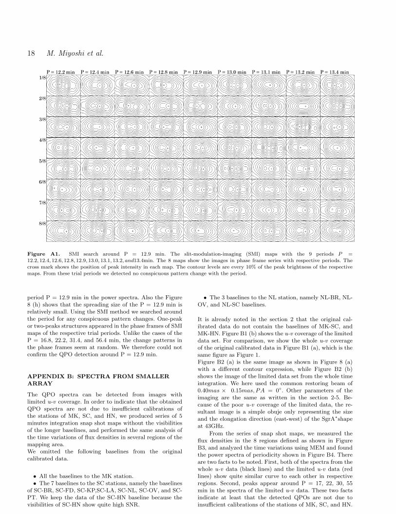
Figure A1. SMI search around P = 12.9 min. The slit-modulation-imaging (SMI) maps with the 9 periods P =

12.2, 12.4, 12.6, 12.8, 12.9, 13.0, 13.1, 13.2, and13.4min. The 8 maps show the images in phase frame series with respective periods. Thecross mark shows the position of peak intensity in each map. The contour levels are every 10% of the peak brightness of the respective

maps. From these trial periods we detected no conspicuous pattern change with the period.

period P = 12.9 min in the power spectra. Also the Figure8 (h) shows that the spreading size of the P = 12.9 min isrelatively small. Using the SMI method we searched aroundthe period for any conspicuous pattern changes. One-peakor two-peaks structures appeared in the phase frames of SMImaps of the respective trial periods. Unlike the cases of theP = 16.8, 22.2, 31.4, and 56.4 min, the change patterns inthe phase frames seem at random. We therefore could notconfirm the QPO detection around P = 12.9 min.

APPENDIX B: SPECTRA FROM SMALLERARRAY

The QPO spectra can be detected from images withlimited u-v coverage. In order to indicate that the obtainedQPO spectra are not due to insufficient calibrations ofthe stations of MK, SC, and HN, we produced series of 5minutes integration snap shot maps without the visibilitiesof the longer baselines, and performed the same analysis ofthe time variations of flux densities in several regions of themapping area.We omitted the following baselines from the originalcalibrated data.

• All the baselines to the MK station.• The 7 baselines to the SC stations, namely the baselines

of SC-BR, SC-FD, SC-KP,SC-LA, SC-NL, SC-OV, and SC-PT. We keep the data of the SC-HN baseline because thevisibilities of SC-HN show quite high SNR.

• The 3 baselines to the NL station, namely NL-BR, NL-OV, and NL-SC baselines.

It is already noted in the section 2 that the original cal-ibrated data do not contain the baselines of MK-SC, andMK-HN. Figure B1 (b) shows the u-v coverage of the limiteddata set. For comparison, we show the whole u-v coverageof the original calibrated data in Figure B1 (a), which is thesame figure as Figure 1.Figure B2 (a) is the same image as shown in Figure 8 (a)with a different contour expression, while Figure B2 (b)shows the image of the limited data set from the whole timeintegration. We here used the common restoring beam of0.40mas × 0.15mas, PA = 0◦. Other parameters of theimaging are the same as written in the section 2-5. Be-cause of the poor u-v coverage of the limited data, the re-sultant image is a simple obuje only representing the sizeand the elongation direction (east-west) of the SgrA∗shapeat 43GHz.

From the series of snap shot maps, we measured theflux densities in the 8 regions defined as shown in FigureB3, and analyzed the time variations using MEM and foundthe power spectra of periodicity shown in Figure B4. Thereare two facts to be noted. First, both of the spectra from thewhole u-v data (black lines) and the limited u-v data (redlines) show quite similar curve to each other in respectiveregions. Second, peaks appear around P = 17, 22, 30, 55min in the spectra of the limited u-v data. These two factsindicate at least that the detected QPOs are not due toinsufficient calibrations of the stations of MK, SC, and HN.

c© 20** RAS, MNRAS 000, 1–??

Oscillation in SgrA∗ 19

Figure B1. The u-v coverages of the whole calibrated data (a) and the limited data (b). The Figure B 2 (a) is the same plot as Figure1.

Figure B2. maps

APPENDIX C: CALCULATED CLOSUREPHASES FROM THE SMI MAPS (P =16.8 MIN)

In Figure C 1 and 2, we show the closure phases calculatedfrom the 8 maps from the SMI method at P= 16.8 min.The SMI maps show consistent closure phases to the ob-served ones. First of all, the small triangles containing FD,LA, PT, KP, and OV stations shows nearly zero, constantclosure phases both in observed closures and the calculatedones. Second, the observed closure phases of triangles con-taining one station from BR or NL and two stations from theinner five stations FD, LA, PT, KP, and OV show deviations

of a few tens of degrees from zero. The calculated closurephases from the SMI maps show different values from theobserved ones, however, the distributions of them cover theregions of variations of the observed closure phases. Third,the larger the triangles become, the observed closure phasesshow larger deviations up to ±180◦. The calculated closurephases from the SMI maps also show the same large devia-tions. From the point of closure phases, the SMI maps showconsistent behavior to the observed closure phases.

c© 20** RAS, MNRAS 000, 1–??

20 M. Miyoshi et al.

Figure B3. The definition of the 8 regions. The size of region (4) is comparable to so called a scattering size of SgrA∗at 43GHz. Assumingthe distance to the Galactic center to be 8 kpc and the mass of SgrA∗to be 4 × 106Msun, the apparent 3 mas corresponds to be 24 AU,

or 305 Schwarzschild radii.

Figure B4. The power spectra of the periodicities in the 8 regions. Black line shows the spectrum obtained from the whole calibrateddata, red line shows the spectrum obtained from the limited calibrated data.

c© 20** RAS, MNRAS 000, 1–??

Oscillation in SgrA∗ 21

Figure C1. The calculated closure phases from the eight SMI maps (P =16.8 min) (1/2).

c© 20** RAS, MNRAS 000, 1–??

22 M. Miyoshi et al.

Figure C2. The calculated closure phases from the eight SMI maps (P =16.8 min) (2/2)

.

c© 20** RAS, MNRAS 000, 1–??

Oscillation in SgrA∗ 23

APPENDIX D: IMAGES WITH SEVERALLIMITED VISIBILITY SETS

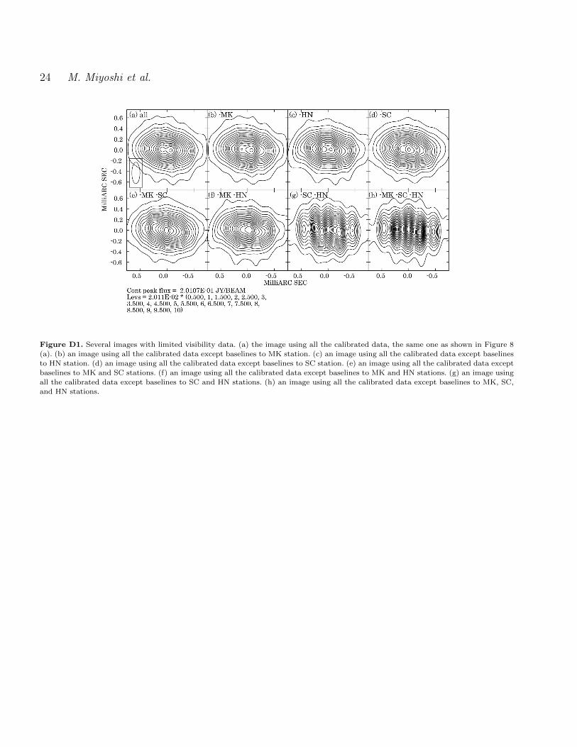
Figure D shows several images from the whole time integra-tion with several limited visibility sets. Here we performedimagings with the task IMAGR with the same parametersas described in the section 2-5. Visibility data from the base-lines to MK seem to do almost nothing to the image quality.The 4 images without the baselines to MK, (b), (d), and (e)in Figure D, are very similar to each other and also to theimage from all data, (a) in Figure D. While the existences ofthe baselines to HN, and SC in data play fairly an importantrole to the imaging quality. The exception of one from thetwo stations gives little influence to the image quality ((c),(d), (e), (f), (g) in Figure D). The exception of both of theHN, SC stations gives quite a degree of influence in imagequality ((g), and (h) in Figure D).

c© 20** RAS, MNRAS 000, 1–??

24 M. Miyoshi et al.

Figure D1. Several images with limited visibility data. (a) the image using all the calibrated data, the same one as shown in Figure 8

(a). (b) an image using all the calibrated data except baselines to MK station. (c) an image using all the calibrated data except baselines

to HN station. (d) an image using all the calibrated data except baselines to SC station. (e) an image using all the calibrated data exceptbaselines to MK and SC stations. (f) an image using all the calibrated data except baselines to MK and HN stations. (g) an image using

all the calibrated data except baselines to SC and HN stations. (h) an image using all the calibrated data except baselines to MK, SC,

and HN stations.

c© 20** RAS, MNRAS 000, 1–??