PHYSICAL REVIEW E 89, 053016 (2014)

Oscillating-grid experiments in water and superfluid helium

Rose E. Honey, Robert Hershberger, and Russell J. Donnelly*

Department of Physics, University of Oregon, Eugene, Oregon 97403, USA

Diogo BolsterDepartment of Civil Engineering and Geological Sciences, University of Notre Dame, Indiana 46556, USA

(Received 16 December 2013; published 19 May 2014)

Passing a fluid through a grid is a well-known mechanism used to study the properties of turbulence. Oscillatinga horizontal grid vertically in a tank has also been used extensively and is considered to be a source of almosthomogenous isotropic turbulence. When the oscillating grid is turned on a turbulent flow is induced. A fronttranslates into the experimental tank, behind which the flow is highly turbulent. Long predicted that the growth ofsuch a front would grow diffusively as the square root of time (i.e., d ∼ √

t) and Dickinson and Long presentedexperimental evidence for the diffusive result at a low mesh Reynolds number of 555. This paper revisits theseexperiments and attempts a set of two models for the advancing front in both square and round tanks. We do notobserve significant differences between runs in square and round tanks. The experiments in water reach meshReynolds numbers of order 30 000. Using some data from superfluid helium experiments we are able to exploremesh Reynolds numbers to about 43 000. We find the power law for the advancing front decreases weakly with themesh Reynolds number. Using a very long tank we find that the turbulent front stops completely at a certain depthand attempt a simple explanation for that behavior. We study the propagation of the turbulent front into tubesof different diameters inserted into the main tank. We show that these tubes exclude wavelengths much largerthan the tube diameter. We explore the variation of the position of the steady-state boundary H on tube diameterD and find that H = cD with c ∼ 2. We suggest this may be explained by saturation of the energy-containinglength scale �e. We also report on the effect of plugging up just one hole of the grid. Finally, we recall someearlier oscillating grid experiments in superfluid 4He in the light of the present results.

DOI: 10.1103/PhysRevE.89.053016 PACS number(s): 47.27.Gs

I. INTRODUCTION

Rouse and Dodu [1] appear to be the first to use oscillatinggrids as a source of zero-mean-shear turbulence for studyingturbulent mixing and dispersion in homogeneous, stratified,rotating, or two-phase fluids. Thompson and Turner [2]studied scales of velocity and length in the fluid near themixing interface. Dickinson and Long [3] and Hopfingeret al. [4] have measured the speed of propagation of tur-bulent fronts generated by oscillating grids in homogeneousfluids with and without rotation. Ivey and Corcos [5] haveused oscillating grids to study boundary mixing in stratifiedfluids.

Oscillating grids are considered to be a source of almosthomogenous isotropic turbulence. Careful discussion of themethods needed to achieve this have been given by De Silvaand Fernando [6] (which includes a thorough literature survey),Fernando and De Silva [7], and Voropayev and Fernando [8].When the oscillating grid rig is turned on a turbulent flow isinduced. A front translates into the experimental tank, behindwhich the flow is highly turbulent. Long [9] predicted that thegrowth of such a front would vary diffusively as the squareroot of time (i.e., d ∼ √

t). In this work, which attractedconsiderable interest, Long modeled the induced flow as asystem of point source-sink doublets of opposite sign arrangedregularly in the plane of the grid. However, this model flow isirrotational, which is clearly not true for a turbulent flow.

*rjd@uoregon.edu

The present paper describes the apparatus for visual andphotographic analysis of the experiments in water. This paperpresents two simple models for describing the advance of theturbulent front after starting the grid into oscillation in bothsquare and round tanks and for several mesh sizes. It is foundthat the advance of the front can be described by a power lawbut that the exponent in the long-time decay depends weakly onthe mesh Reynolds number. An earlier power law immediatelyfollowed on starting the grid into oscillation is also reportedand its transition to long-time decay is found to be quite sharp.

We pursue the propagation of the front into a much deepertank, and we discover that the front does not continue travelingdown but stops at a definite depth. We advance a simpleexplanation for this phenomenon. We also study the motionof the turbulent front in circular tubes inserted into the tankwith a variety of diameters. We find the circular tubes behaveas a high-pass filter, where the word high refers to eddywave numbers. Eddies with wavelengths larger than the tubediameter are less able to enter. We also describe the effect ofblocking a single mesh hole in an experiment in water. Finally,we discuss some oscillating grid experiments in superfluid 4Hein the light of the present results.

II. EXPERIMENTAL APPARATUS

The apparatus evolved steadily as experience was gathered.In the early stages of this investigation we took the view thatsince we were studying turbulence the apparatus need not beof especially precise design. We know now that every attemptto improve the design yielded better results.

1539-3755/2014/89(5)/053016(11) 053016-1 ©2014 American Physical Society

HONEY, HERSHBERGER, DONNELLY, AND BOLSTER PHYSICAL REVIEW E 89, 053016 (2014)

crank

motor

Acrylic cover

grid origin

bottom of stroke

water surface

Light Source

FIG. 1. Sketch of the experimental apparatus with the drive usedin the early stages of this investigation. This tank had height H =36 cm and width W = 22 cm. This apparatus was used for the datain Tables III–V and Figs. 9–12, and 14.

A. The tanks

Three square tanks of heights H = 36, 46, and 122 cmwere constructed from sheets of 0.953-cm thickness acrylic,solvent welded. A bead of silicone guarded against occasionalwater leaks. Each tank had an inside width of W = 22 cm.We constructed one tank of cylindrical shape with diameter30 cm. Results with the cylindrical design appeared generally

screw holes×4

M

d

FIG. 2. Sketch of the grid design: M = 1.59 cm and d =0.318 cm. The screw holes are for the four support rods.

consistent with the square design and are not reported here. Thegrid is usually placed 6.5 cm below the surface of the water.After a data run we waited some time to ensure equilibrium.We found that evaporation from the free surface drove weakconvective rolls at the top of the tank. Placing a loosely fittingPlexiglas plate between the surface and the grid eliminatedthis problem.

B. The grids

The design of our system is illustrated in Figs. 1, 2, and 3.The oscillation takes place at a frequency f (circular frequencyω = 2πf ). The drive system has a stroke s, which is thedistance the grid moves from bottom to top. The amplitudeof the oscillation is ε = S

2 . Oscillating bars are governed bythe Keuligan-Carpenter number NKC and the Stokes number

FIG. 3. (Color online) Sketch of the improved apparatus. Herethe stepper motor and wheel are replaced by a linear motor (notshown). This apparatus was used for the pictures and data in Figs. 4,5, 6, and 15.

053016-2

OSCILLATING-GRID EXPERIMENTS IN WATER AND . . . PHYSICAL REVIEW E 89, 053016 (2014)

TABLE I. NKC numbers for the 1.59-cm mesh grid.

S (cm) NKC

1 11.52 20.93 31.44 41.95 52.46 62.87 73.38 83.8

St. For reference, these numbers for the grid bars are given inTables I and II. The definitions are

NKC = 2πε

d, (1)

St = f d2

ν, (2)

where d is the thickness of the bars as shown in Fig. 2 and ν

is the kinematic viscosity of the fluid.The characteristic velocity of the grid is Uo = ωε, and the

mesh Reynolds number is

ReM = UoM

ν, (3)

where M is defined as the distance from the center of one barto the center of the next. Our best results (good reproducibility,relatively stable turbulent front) were obtained with the M =1.59 cm, d = 0.318 cm mesh as shown in Fig. 2.

The grid edges end in half a mesh in order to reduce the shearat the walls. The optimum grid design is described by De Silvaand Fernando [6] as follows: “. . .to obtain nearly isotropicturbulence with zero-mean flow, certain design conditions haveto be satisfied: the grid should have a solidity less than 40%,the oscillation frequency should be less than 7 Hz, the endconditions of the grid should be selected to yield low Reynoldsstress gradients and measurements should be taken 2–3 meshsizes away.” The spacing between the ends of the grid tines andthe tank wall is quite small, on the order of 0.025 cm. The halfmesh spacing influenced the generation of large-scale motionin the tank: Typically the turbulent front will become unstableand speed down one side of the tank, a larger gap resultingin more unwanted motion. Also, unequal gaps on oppositesides resulted in greater large-scale motion. Towards the endof this investigation we used a high-precision grid of the samedimensions, machined by a numerically controlled mill. It isillustrated in Fig. 2. It is very important that the support rods

TABLE II. Stokes numbers for the 1.59-cm mesh grid.

f (Hz) St

5 456 547 638 729 8110 90

for the grid are no larger than d. If they are not hidden by thegrid, they will generate their own turbulent flow.

C. The motor drive

The grid support rods are connected as shown in Fig. 1to a stepper motor with a torque of 2.8 N m turning a wheelwith five holes drilled at various radii to provide a four-barlinkage to the grid providing variable frequency of oscillationand strokes s ranging from 1 to 5 cm. The frequency of thedrive can be varied and ranged between 0.5 and 6 Hz.

Recently, we have replaced the stepper motor with a CopleyControls model STA2510S-104-S-S03X linear motor capableof 780 N of peak thrust. The grid supports are directly attachedto the magnet rods of the motors, eliminating mechanicalbacklash. Also, the motors are brushless and ironless, resultingin smoother motion due to minimal motor cogging. The motorsprovide stroke lengths s anywhere between 0 and 10 cm.

The motor is driven by a Copley model XSL-230-18Xenus indexer and amplifiers. Since the motors are brushless,electronic commutation is provided by the Xenus amplifiervia linear Hall-effect sensors mounted on the forcer assembly.These same sensors also provide positional feedback. Thebasic resolution of the motors is 12.5 μm. The Xenusamplifiers are an entirely digital system, allowing readyreprogramming of the feedback loop coefficients, and they alsointernally generate the motion trajectory based on variablessent via an RS-232 link.

We found it advisable to attach the grid apparatus to a heavyplatform supported by a concrete pillar to minimize vibration.

D. Visualization, lighting of the flow, and protocol

We found the problem of visualization of the flow of crucialimportance to this experiment. Our first thought was to use theBaker thymol blue technique for visualization. This provedto give attractive pictures, but was of little use in trackingthe turbulent front in practice. We finally used Kalliroscopeto study the turbulent motions in water. Kalliroscope is acommercial product first described scientifically in a paperby Matisse and Gorman [10]. Exactly what is shown bylight reflection from these anisotropic fish scale particles isstill not entirely clear, although an analytical study by Savas[11] suggests that the flakes align themselves with streamsurfaces with rapid turnovers and further notes that it is auseful technique for determining certain flow patterns. Thesescales align with the direction of shear and, when illuminatedby a light sheet, give a good contrast between turbulent andnonturbulent regions. A discussion by Gauthier, Gondret, andRabaud [12] is very useful in this respect: In particular, theyshow that the observed light cannot be used to reconstructthe velocity field. However, they do show that Kalliroscopecan be used specifically to visualize vortical flow structures bycomparing numerical predictions to experimental observationsin Taylor-Couette flow.

Different lighting methods were tested for visualization.Shining white light through the whole tank caused visualiza-tion of all movement, which blocked the view of the turbulentfront spreading down roughly at the center of the tank. Wefinally adopted a vertically collimated slit of light (1.5 cm

053016-3

HONEY, HERSHBERGER, DONNELLY, AND BOLSTER PHYSICAL REVIEW E 89, 053016 (2014)

wide) from a slide projector shone through the center of thetank from left to right. On setting up the apparatus the length ofthe rod connected to the grid was adjusted so the grid positionat the bottom of the stroke was 6.5 cm below the top cover.Since turbulence was measured from the bottom of the stroke,the stroke s, divided by 2 and subtracted from the 6.5-cm markwould give the mean position of the grid. We took the view thatthe origin of the turbulence was at the bottom of the stroke.Correcting to the mean position of the stroke did not affect theresults in any significant way.

Distances from the grid were measured and marked withtape on two sides of the tank to avoid parallax. The gridwould begin its oscillations (always from its lowest position),creating turbulence which would be revealed by light scatteringfrom Kalliroscope flakes. The boundary between vortical andquiescent fluid was sharp and easy to observe. When theturbulent front reached a given tape mark, the time couldbe recorded electronically. Thus we could make a completerecord of the propagation of the front down the tank in a singlerun. This efficiency allowed us to complete hundreds of runsin a reasonable period of time.

E. Photography of the front

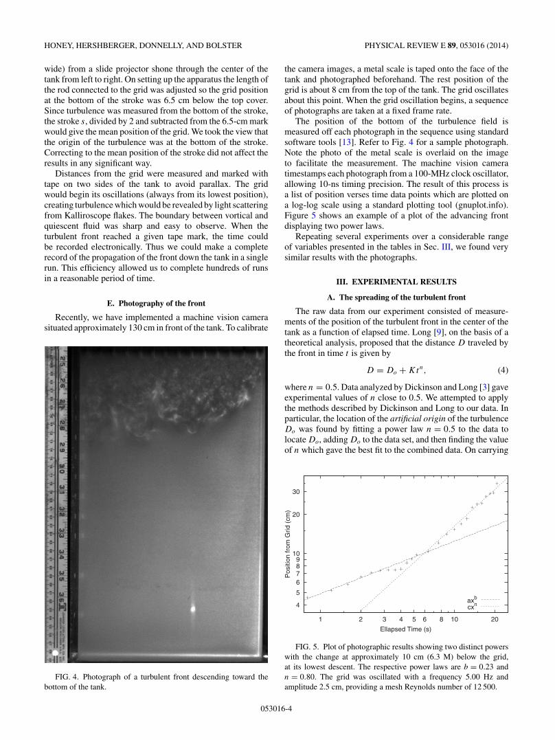
Recently, we have implemented a machine vision camerasituated approximately 130 cm in front of the tank. To calibrate

FIG. 4. Photograph of a turbulent front descending toward thebottom of the tank.

the camera images, a metal scale is taped onto the face of thetank and photographed beforehand. The rest position of thegrid is about 8 cm from the top of the tank. The grid oscillatesabout this point. When the grid oscillation begins, a sequenceof photographs are taken at a fixed frame rate.

The position of the bottom of the turbulence field ismeasured off each photograph in the sequence using standardsoftware tools [13]. Refer to Fig. 4 for a sample photograph.Note the photo of the metal scale is overlaid on the imageto facilitate the measurement. The machine vision cameratimestamps each photograph from a 100-MHz clock oscillator,allowing 10-ns timing precision. The result of this process isa list of position verses time data points which are plotted ona log-log scale using a standard plotting tool (gnuplot.info).Figure 5 shows an example of a plot of the advancing frontdisplaying two power laws.

Repeating several experiments over a considerable rangeof variables presented in the tables in Sec. III, we found verysimilar results with the photographs.

III. EXPERIMENTAL RESULTS

A. The spreading of the turbulent front

The raw data from our experiment consisted of measure-ments of the position of the turbulent front in the center of thetank as a function of elapsed time. Long [9], on the basis of atheoretical analysis, proposed that the distance D traveled bythe front in time t is given by

D = Do + Ktn, (4)

where n = 0.5. Data analyzed by Dickinson and Long [3] gaveexperimental values of n close to 0.5. We attempted to applythe methods described by Dickinson and Long to our data. Inparticular, the location of the artificial origin of the turbulenceDo was found by fitting a power law n = 0.5 to the data tolocate Do, adding Do to the data set, and then finding the valueof n which gave the best fit to the combined data. On carrying

4

5

6789

10

20

30

1 2 3 4 5 6 8 10 20

Pos

ition

from

Grid

(cm

)

Ellapsed Time (s)

axb

cxn

FIG. 5. Plot of photographic results showing two distinct powerswith the change at approximately 10 cm (6.3 M) below the grid,at its lowest descent. The respective power laws are b = 0.23 andn = 0.80. The grid was oscillated with a frequency 5.00 Hz andamplitude 2.5 cm, providing a mesh Reynolds number of 12 500.

053016-4

OSCILLATING-GRID EXPERIMENTS IN WATER AND . . . PHYSICAL REVIEW E 89, 053016 (2014)

TABLE III. Data fitted to D = Do + Ktn for the square tank.Notes: Each set consisted of the average of 10 trials with the resultsfor the times at each position averaged together. Thus 3 represents 30trials and 10 represent 100 trials. χ 2 is the usual statistical measureof goodness of fit.

M (cm) f (Hz) S (cm) n K Do (cm) χ 2 sets

0.36 5.0 2.0 0.42 9.028 −7.70 0.157 30.36 5.0 5.0 0.35 24.20 −20.15 0.146 10.51 5.0 2.0 0.66 4.73 −3.34 0.059 30.51 5.0 5.0 0.57 13.71 −9.20 0.105 10.85 5.0 2.0 0.53 7.29 −7.05 0.022 30.85 5.0 5.0 0.66 12.93 −8.31 0.101 11.59 2.5 2.0 0.47 6.65 −6.59 0.120 101.59 3.75 2.0 0.62 4.73 −2.78 0.040 11.59 5.0 1.0 0.51 3.76 −3.40 0.018 101.59 5.0 2.0 0.45 10.8 −8.94 0.195 101.59 5.0 4.0 0.19 39.8 −36.1 0.108 101.59 5.0 5.0 0.24 35.8 −31.14 0.128 11.59 6.25 1.0 0.48 4.66 −4.02 0.045 11.59 6.25 2.0 0.59 7.60 −4.97 0.126 11.59 6.25 4.0 0.39 21.12 −17.37 0.071 11.59 6.25 5.0 0.24 40.71 −35.31 0.183 11.59 7.5 2.0 0.38 18.1 −16.20 0.191 10

this out we, too, found a power law near 0.5. However, usinga power law of 0.4 to find Do gave a fit with n near 0.4, andusing a power law of 0.6 to find Do gave a fit with n near 0.6.We concluded that this method was not suitable for our data.

The safest procedure, we believe, is to simply fit the dataset directly to (4) and record the best fit values of K , n, andDo. This has been carried out in Table III for the square tank.We have a complete set of experiments in round tanks, butthe data did not substantially differ from square tanks and isomitted here.

Analysis with Eq. (4) showed that the artificial origin of theturbulence is located above the grid and can be many meshlengths long. We therefore tried another simple model,

D = K(t − to)n, (5)

with t > to. The results of this analysis are shown in Table IVfor the square tank. As can be seen (5) gives a much morereasonable result, with to of order 1 s, compared with a runduration 10 to 60 s. Indeed, we did two more analyses takingto to be 1 s and its average to be 1.3 s. This was an attemptto reduce the number of variables being found by the fittingroutine. We do not reproduce these analyses here, for they didnot appear to have any obvious advantage over the fits shownin Tables IV and V.

We also display in Table V the mesh Reynolds numberdefined in Eq. (3). Examination of some data concentratedin the first 10 cm or so revealed that the data in this rangeare simply linear in time. In order to explore this further weomitted data in the first 10 cm and reanalyzed the data as shownin Table V for the square tank.

Comparison of the χ2 values between Tables IV and Vdemonstrate that a great improvement in the fit is obtained inthis way. We conclude that something different is going on inthe first few seconds of the experiment, perhaps the jets being

TABLE IV. Data fitted to D = K(t − to)n for the square tank.

M (cm) f (Hz) S (cm) n K to (s) χ 2 Sets

0.36 5.0 2.0 0.52 5.26 1.43 0.074 30.36 5.0 5.0 0.53 10.58 0.96 0.084 10.51 5.0 2.0 0.70 3.88 0.97 0.044 30.51 5.0 5.0 0.66 9.77 0.76 0.074 10.85 5.0 2.0 0.62 4.62 1.47 0.006 30.85 5.0 5.0 0.78 9.16 0.57 0.158 11.59 2.5 2.0 0.57 3.90 1.70 0.196 101.59 3.75 2.0 0.67 3.74 0.66 0.057 11.59 5.0 1.0 0.57 2.71 1.85 0.037 101.59 5.0 2.0 0.58 5.99 1.02 0.311 101.59 5.0 4.0 0.45 9.46 0.94 0.441 101.59 5.0 5.0 0.49 10.95 0.90 0.212 11.59 6.25 1.0 0.48 4.22 4.12 0.123 11.59 6.25 2.0 0.68 5.41 0.65 0.172 11.59 6.25 4.0 0.62 9.06 0.73 0.215 11.59 6.25 5.0 0.50 11.86 0.83 0.323 11.59 7.5 2.0 0.57 7.76 1.05 0.358 10

produced by the grid take some time to organize themselvesinto a more homogeneous type of turbulence, which is whatwe saw in earlier investigations. A paper by Voropayev andFernando [8] describes the evolution of the flow from themultipolar flow in each hole in the mesh to a distance downthe tank where the jets from all the holes interact and start tomake a turbulent flow. The authors cite Hinze [14] as the sourceof the transition at about 20M . We have been able to shed somelight on this process by recording the flow photographically.

We show some results in Fig. 5 in which the front movesdown the tank a distance ∼10 cm in about 4 s and has a powerlaw f (x) = axb with b = 0.23 followed by a distinct changein power law f (x) = cxn with n = 0.80. This change occursat a distance 10 cm or 10/M = 6.3M .

TABLE V. Data fitted to D = K(t − to)n for the square tankomitting data below 10 cm.

M (cm) f (Hz) S (cm) n K to (s) χ 2 Sets ReM

0.36 5.0 2.0 0.56 4.49 0.51 0.026 3 23000.36 5.0 5.0 0.48 11.84 1.22 0.0008 1 57000.51 5.0 2.0 0.77 3.10 0.05 0.0005 3 32000.51 5.0 5.0 0.59 11.29 1.05 0.022 1 80000.85 5.0 2.0 0.64 4.42 1.28 0.006 3 53000.85 5.0 5.0 0.65 11.68 0.95 0.035 1 13 4001.59 2.5 2.0 0.50 5.14 3.66 0.036 10 50001.59 3.75 2.0 0.62 4.45 1.41 0.054 1 75001.59 5.0 1.0 0.53 3.15 3.57 0.008 10 50001.59 5.0 2.0 0.49 7.80 2.08 0.085 10 10 0001.59 5.0 4.0 0.39 11.15 1.52 0.141 10 20 0001.59 5.0 5.0 0.43 12.46 1.24 0.095 1 25 0001.59 6.25 1.0 0.51 3.74 3.11 0.027 1 62001.59 6.25 2.0 0.57 7.39 1.62 0.105 1 12 5001.59 6.25 4.0 0.54 10.79 1.09 0.105 1 25 0001.59 6.25 5.0 0.42 14.07 1.21 0.029 1 31 2001.59 7.5 2.0 0.48 9.77 1.75 0.114 10 15 000

053016-5

HONEY, HERSHBERGER, DONNELLY, AND BOLSTER PHYSICAL REVIEW E 89, 053016 (2014)

0

0.2

0.4

0.6

0.8

1

0 5 10 15 20 25 30 35 40 45

n

103 Rem

FIG. 6. Results for the power exponent n in Eq. (2) as a functionof mesh Reynolds number from Table V in a square tank. The highestmesh Reynolds number point is taken from Smith’s thesis [15] usingliquid helium and the range of possible fits is given by the vertical bar.The experiments of Dickinson and Long [3] were at a mesh Reynoldsnumber of 555 and are shown as a triangle. The trend line is given byn = 0.594 − 0.005 05 × ReM .

B. Results for the long-time power law as a functionof mesh Reynolds number

We were unable to reproduce the results of Dickensonand Long [3] whereby the turbulent front spreads diffusively.Instead we find the power law described by n is a slow functionof mesh Reynolds number over a great range of Reynoldsnumbers as shown in Fig. 6.

The large scatter seen in Fig. 6 reflects the fact that thepropagating front in this type of experiment is often veryunstable. The front tends to move to one side of the tankand plunge rapidly to the bottom. This behavior is perhapsthe greatest limitation to this type of experiment. The highestmesh Reynolds number point is described in Sec. VII B.

IV. STATIONARY TURBULENT FRONTS IN SMALLERDIAMETER TUBES

We report on observations of the steady-state turbulentboundary in an oscillating grid experiment. We find that in asufficiently deep tank the oscillating grid does not completelyfill the tank with turbulence, even after long times. Instead,there is a boundary between turbulent and nonturbulent regionsat a definite distance from the oscillating grid. We explore thevariation of the position of the steady-state boundary H ontube diameter D and find that H = cD with c ∼ 2.

To observe the behavior of turbulence in different sizecontainers, we hang Plexiglas tubes of various diameters D

(0.6 cm < D < 17 cm) in the main tank. The tubes have awall thickness of 0.3 cm. They are supported by a simple rigidharness that spans the width of the tank well below the regionwhere turbulence exists in the tubes. The harness is suspendedby strings that clip onto the top edges of the walls of the tank.With this system, we are able to position the tube anywhere inthe tank and at any height. We usually make our measurementswith the tube near the center of the tank. The tubes are typically50 cm long, with the top end open and the bottom end plugged.

0

10

20

30

40

50

1 2 3 4 5 6 7

Dep

th o

f fro

nt (

cm)

Frequency (Hz)

inside the tubeoutside the tubeno tube in tank

FIG. 7. Depth of the turbulent front in steady state in an oscillatinggrid experiment. The tube used in this experiment was 10 cm indiameter. This experiment shows that the presence of the tube did notdisturb the turbulence in the main tank.

To illustrate the observations, Fig. 7 shows the steady-stateturbulent boundary as a function of oscillation frequency forthe empty tank and for a 10-cm-diameter tube placed in thetank. The tube was placed just off center. We measure thedepth simply by estimating by eye the edge of the turbulentregion and measuring with a ruler the distance between thispoint and the midpoint of the grid stroke. The measurementis made difficult by the fact that the boundary is undulatingacross the width of the tank, reflecting the wide range of eddysizes that make up the turbulence. The boundary advancesand retreats in the tube over time suggesting intermittency.We attempt to identify the average position of the boundary.The measurements are made after waiting 10–15 min afterturning on the grid motor to ensure that the boundary is nolonger advancing. We have compared the depths measuredafter waiting 15 min to depths measured after waiting 1 h andfound no difference within experimental error. To investigatethis phenomenon further we devised the measurement shownschematically in Fig. 8.

A tube of diameter D hung a distance L below the grid willmeasure a penetration depth h, which is the distance betweenthe mouth of the tube and the boundary between turbulent andnonturbulent regions in the tube. We record h for a varietyof values of L and calculate the total depth of the boundaryH = L + h. If the distance that the turbulence propagates inthe tube depends in some way on the interaction with the tube,then measurements made at different values of L will notrecover the same H . For example, if the turbulent energy inthe tube were primarily generated at the tube mouth, perhapsby vorticity generation at the edges, then one would expect thepenetration depth h to be a constant, independent of L.

We used hanging heights of L = 4 to 10 cm. The grid wasoscillated at 1, 3, and 5 Hz with a stroke of 1.5 cm. As expected,the penetration increases with frequency and with closenessto the grid. Figures 9–12 show the total depth H calculatedby adding h to L. For each frequency a reasonably constantvalue of H is measured. A crude measure of the collapse isgiven by the dimensionless spread H/H ≈ 0.1 in Fig. 9 to

053016-6

OSCILLATING-GRID EXPERIMENTS IN WATER AND . . . PHYSICAL REVIEW E 89, 053016 (2014)

gridL1

h1

D

L2

h2

D

L3

h3

D

H

turbulence front

FIG. 8. Schematic illustration of the measurement of the turbu-lence front in a tube hung in the tank at different depths L.

H/H ≈ 1 in the smallest tube in Fig. 12. While the errors arerather large (∼±10%) and the data do not collapse perfectly,there does not seem to be any systematic variation with L.

Figure 12 shows rather poor collapse of the H data anda systematic variation with L, indicating that the tube isaffecting the measurement. We found that for tube diameterslarger than 3 cm there is generally good collapse of the dataand the H measurement was meaningful. For smaller tubediameters the measurement was not meaningful. It is knownthat closer than 2–3 mesh lengths to the grid the flow is

9

10

11

12

13

14

15

16

17

0 1 2 3 4 5 6

H (

cm)

Frequency (Hz)

L = 4.1 cm L = 6.1 cm L = 7.7 cm L = 9.0 cm L = 9.7 cm

FIG. 9. Depth of steady-state turbulent front in a tube 5.7 cminner diameter for various frequencies. The collapse of H is quitegood for this larger tube. Here H/H ≈ 0.1.

5

6

7

8

9

10

11

12

1 2 3 4 5

H (

cm)

Frequency (Hz)

L = 4.2 cm L = 6.0 cm L = 7.0 cm L = 7.8 cm

FIG. 10. Depth of the steady-state turbulent front in a tube of3.17-cm inner diameter for various frequencies. The collapse is stillgood for this diameter tube, H/H ≈ 0.2.

dominated by jets produced by the grid [14]. Only further fromthe grid do the jets merge to form homogeneous turbulence.Therefore, we should not expect reasonable results closer than∼5 cm to the grid [14]. In fact our own measurements asseen in Fig. 5 suggest a distance ∼10 cm might be moreappropriate.

V. ENERGY SPECTRUM: HIGH-PASS FILTER

It is not surprising that the turbulent front reaches asteady-state depth. As the turbulence travels away from thegeneration region next to the grid, the turbulent energy decaysvia the energy cascade and viscous dissipation. At somedepth, the turbulent energy should decay to zero and thefront can no longer propagate. The smaller the diameter ofthe tubes the less we expect the front to descend as wasobserved in the experiments. The reason for this is thatsmaller diameters exclude the turbulent energy at larger scales.Essentially, the tube acts as a filter, excluding eddies larger than

3

3.5

4

4.5

5

5.5

6

6.5

7

0 1 2 3 4 5 6

H (

cm)

Frequency (Hz)

L = 3.0 cm L = 4.0 cm L = 5.0 cm L = 6.0 cm

FIG. 11. Depth of the steady-state turbulent front in a tube of1.6-cm inner diameter for various frequencies. Here H/H ≈ 0.8.

053016-7

HONEY, HERSHBERGER, DONNELLY, AND BOLSTER PHYSICAL REVIEW E 89, 053016 (2014)

0

0.5

1

1.5

2

2.5

3

0 1 2 3 4 5 6

H (

cm)

Frequency (Hz)

L = 0.3 cm L = 1.0 cm L = 1.5 cm

FIG. 12. Depth of the steady-state turbulent front in a tube of0.6-cm inner diameter for various frequencies. The data do notcollapse for this small diameter tube, H/H ≈ 1.

the tube diameter. The decay of turbulence becomes fasterwhen the energy containing length scale �e of the turbulencebecomes comparable to the length scale of the container [16].Therefore, in the oscillating grid experiment we expect theenergy containing length scale to be comparable to that of thetank or tube, after which accelerated decay of turbulence willoccur,

�e =(

3π

4

)∫ ∞2πD

k−1 E(k) dk∫ ∞2πD

E(k) dk. (6)

We have ignored viscous effects in the above equation byleaving the upper limit of integration as ∞. We define theenergy containing wave number as ke = 2π/�e. For smallwave numbers (k � ke) we use E(k) = Ak2 and for thelarge wave numbers (k � ke) we use the Kolmogorov lawE(k) = Cε2/3k−5/3. This gives

�e =(

3π

4

) 1110k2

e − 12

(2πD

)2

116 k3

e − 13

(2πD

)3 . (7)

0

0.5

1

1.5

2

2.5

3

0 1 2 3 4 5 6 7 8 9 10

E(k

) (a

rb. u

nits

)

k (arb. units)

kc

ke0

k ≤ kc:

kc ≤ k ≤ ke:

ke ≤ k ≤ kη:

k > kη:

E(k) = 0

E(k) = A km

E(k) = C ε(t)2/3 k-5/3

E(k) = 0

ke

t > tst = tst < tst = 0

FIG. 13. Energy spectrum in a finite channel after Stalp et al. [16].

0

5

10

15

20

25

30

35

0 5 10 15 20

H (

cm)

D(cm)

f = 1.0 Hz f = 3.0 Hz f = 5.0 Hz

FIG. 14. Measurement of H as a function of tube diameter forthree oscillation frequencies. The solid line represents Eq. (8).

We can determine the depth at which the energy containinglength scale is the same as the characteristic length scale ofthe container D. This depth is given by the sole real root ofthe cubic equation above,

�e = 2πD

3.429= 1.83D, (8)

and in this experiment le is identified with H and D is takenas the diameter of the tube (Fig. 13).

Once the turbulence reaches this depth the energy decaysrapidly. If the faster decay is sufficiently rapid we expect theturbulent front to be close to this depth. In Fig. 14 we comparethis depth to the depth of the steady-state turbulent front fromthe experiments. Overall the data appear consistent with thishypothesis, except for the largest-diameter tubes at the smallerforcing frequencies.

VI. ANOMALOUS JET FORMATION

During the initial setup of the experiments we noticed theformation of a jetlike structure that propagated down wellbeyond the turbulent front described in the previous two sub-sections of this paper. Upon further investigation we noticedthat this structure was formed from a region where the mesh didnot maintain the same structure as elsewhere. By plugging upone of the holes in the mesh we saw that such a jet was formed,as illustrated in Fig. 15. This fast-moving plume overtakes themain turbulent front and one possible explanation is that it isa vortex street such as we reported coming from an oscillatingpendulum in Ref. [17], except that the street is turbulent. Ref-erence [17] shows that the damping of a pendulum oscillatingin water is influenced by the emission of vortex rings.

VII. GRID TURBULENCE EXPERIMENTSIN SUPERFLUID 4He

A. Quantized vortex lines

Liquid 4He above the λ transition (2.1768 K) is a perfectlyclassical fluid hydrodynamically and is called helium I. Belowthe λ transition helium II obeys a pair of equations: one for thenormal viscous fluid having density ρn and velocity vn and one

053016-8

OSCILLATING-GRID EXPERIMENTS IN WATER AND . . . PHYSICAL REVIEW E 89, 053016 (2014)

FIG. 15. Photograph of the fast-moving plume generated whenthe central hole in the grid is plugged and is much wider than themesh size M . The rapid motion of this flow suggests that it mightarise from a street of vortex rings such as we reported in Ref. [17],except that the rings are turbulent. The mesh used to generate thisimage is as described in Fig. 2. The top of this image shows a totalwidth of 13M ≈ 20.7 cm.

for the superfluid, an absolutely inviscid fluid, having densityρs and velocity vs . The total density ρ is the sum of the normaland superfluid densities which are separately strong functionsof temperature. The equations of motion for the velocity fieldsdepend on the entropy S of the fluid and the Kelvin temperatureT . The equations of motion yield two forms of “sound,” anordinary wave having density fluctuations and another wavecalled “second sound” exhibiting entropy fluctuations. Moredetailed experiments at Leiden showed that under certain

circumstances an extra term was needed to couple the velocityfields of the two fluids which was called “mutual friction.” Theunderlying physics of mutual friction was investigated later byW. F. Vinen and H. E. Hall in Cambridge (see, for example,Ref. [18]).

When helium II is set into rotation at angular velocity �

the superfluid cannot rotate in the classical sense becausethe superflow is irrotational in a simply connected region.Nevertheless, the entire fluid does rotate, seemingly classically,but the reason is that the superfluid generates a uniform arrayof quantized vortices each with circulation κ = h/m where h

is Plank’s constant and m is the (bare) mass of the helium atom.The vorticity of the rotating superfluid is ω = 2�, the same asthe vorticity in a classical fluid in a rotating container. Whilequantized vortices were suggested theoretically by Onsagerand Feynman [19] no experimental evidence appeared untilVinen and Hall did their thesis work in Cambridge in themid-1950s.

The pioneering experiments in the turbulent flow of heliumII were carried out at Cambridge in helium II by W. F. Vinenand reported in a series of four papers which appeared in 1957[20–23]. When turbulence is present, which Vinen inducedusing a heater at one end of a channel, quantized vortex linesare generated and can tangle together but remain quantizedwith circulation κ = h/m, where h is Planck’s constant andm is the mass of the helium atom. It was only during thisinvestigation that the role of quantized vortex lines was realizedand experiments by Vinen and Hall provided insight into theirbehavior. The remarkable thing is that in a turbulent flow,in contrast to turbulence in ordinary fluids such as waterand air, all vortices have the same size and same quantizedcirculation. This makes a major simplification in the studyof turbulence. Unfortunately, when turbulence is present, thequantized vortices interact with the normal fluid. The only wayto get around this problem is to take advantage of the fact thatthe normal fluid density decreases with temperature and seekto use the lowest temperatures available. For many years thisstudy was called “superfluid turbulence,” but on realization thatif Planck’s constant were zero, the field would not exist, andthe name “quantum turbulence” is now in common use [24,25].

When turbulence is present in helium II in the form of a tan-gle of quantized vortex lines, second sound is attenuated, andby measuring the attenuation one can deduce the magnitude ofthe vorticity in the superfluid [18]. Vorticity in the superfluidcouples the two velocity fields, and the two fluids act as oneby mutual friction; indeed the kinematic viscosity above 1 Kand at larger scales is approximately the viscosity divided bythe total density.

Experiments with towed and oscillating grids in superfluid4He have been carried out for a number of years at theUniversity of Oregon. In particular, Michael Smith presenteda Ph.D. thesis in 1992 with observations on the vorticity ofthe superfluid induced by a towed grid and an oscillating grid[15]. Steven Stalp then took over the apparatus, presentinghis thesis in 1998 [26]. Normally, we would be reluctant tocompare data taken below the λ transition to experimentsin water because the hydrodynamics of helium II require atwo-fluid set of equations. However, Smith reports that hisresults are independent of temperature and viscosity, so as aguess we take the kinematic viscosity of liquid helium at 2.13 K

053016-9

HONEY, HERSHBERGER, DONNELLY, AND BOLSTER PHYSICAL REVIEW E 89, 053016 (2014)

pump

square channel

grid

sliding seal

motor

transducer pair

channel thermometer

liquid helium

FIG. 16. (Color online) Sketch of the apparatus used by Smith tostudy towed grid experiments in helium II [15]. The second-soundtransducers are directly across from each other: one generates secondsound and one detects it. The thermometer was fed to an electronictemperature controller.

(his highest temperature), which is approximately ν = 1.38 ×10−4 cm2/s. Smith had f = 3.75 Hz, M = 0.20 cm, andε = 1.25 cm, giving, finally, n = 0.435 at ReM = 4.27 × 104.

Smith’s apparatus is sketched in Fig. 16, and one of his griddesigns is shown in Fig. 17.

10.0

10.0

1.0

0.52.0

0.5

Rod

FIG. 17. Sketch of one of the sliding grid configurations used bySmith [15], where the dimension is millimeters.

0

5

10

15

20

0 5 10 15 20 25 30

ωrm

s (H

z)

Time (s)

x = 2.11 cmx = 2.41 cmx = 3.02 cm

FIG. 18. Typical averaged signal for the oscillating grid. The threevalues of x illustrate the effects of varying x and the steady-statevorticity. Note that the sharp front does not look like a diffusiveprocess [15].

The sliding grid apparatus has been described in detailin Smith’s and Stalp’s theses [15,26] and in other papers[27]. Briefly, the channel is a 1 cm × 1 cm brass channel,40 cm long. The grid is actuated by a stepping motor mountedoutside the cryostat. Most of the experiments were initiated bysweeping the grid the full length of the channel and monitoringthe decay by attenuation of second sound, which can beinterpreted as giving the vorticity averaged over about 1 cm3.This averaging results in a quiet signal which can be followedover about 6 decades of vorticity.

B. Oscillating grid experiments in helium II

Once the first results with this apparatus were understood,it seemed sensible to try an oscillating grid. Our experimentscould be conducted down to about 1.2 K. Oscillating gridexperiments in the difficult range below 1 K, and indeed to

1

1.2

1.4

1.6

1.8

2

1 1.5 2 2.5 3

Tim

e, t0.

435

Distance (cm)

FIG. 19. Smith’s data fitted to x ∼ tn with the best fit yieldingn = 0.435. But Smith also states that a fit to n = 0.333 looks justas good. The results were found to be independent of temperature,suggesting the two fluids are locked together [15].

053016-10

OSCILLATING-GRID EXPERIMENTS IN WATER AND . . . PHYSICAL REVIEW E 89, 053016 (2014)

0

5

10

15

20

25

30

0 2 4 6 8 10 12

ωrm

s (H

z)

Distance (cm)

FIG. 20. Steady-state vorticity for the oscillating grid as afunction of distance in helum II. The channel was 1 cm × 1 cm.The abscissa is the mean distance the second-sound tranducersare from the oscillating grid. For ω > 4 Hz the solid line ω(x) =113 exp(− x

1.39 ) describes the data fairly well, but we do not understandthe physical basis for this behavior [15].

millikelvin temperatures have been reported in a series ofpapers from McClintock’s group at the University of Lancaster[28–31].

The oscillating grid was driven by a roughly triangularwaveform. Results at three different distances from the grid tothe transducers are shown in Fig. 18. The sharp leading edgeof the received signal suggests a propagating pulse and not adiffusive process, as suggested by Long [9] for classical fluids.Taking the averaged vorticity as a function of x resulted in thedata of Fig. 19. Like the experiments in Sec. III, the turbulent

front ceases to spread after a finite distance (Fig. 20). However,the channel size is 1 cm, so the front is reaching about fivechannel widths instead of the one or two that we see in Fig. 9.At first we speculated that the central post in the grid seen inFig. 17 might be sending a fast-moving plume such as we seein Fig. 15. However, if that were true we should see two frontsarriving at different times. There is no such phenomenon inthe data of Fig. 18, so no definite conclusion can be reached atthis time.

VIII. DISCUSSION

Turbulence generated by grids is now quite an old subjectstarting in the 1940s and continuing ever since. The newerstudy of quantum turbulence has greatly extended our knowl-edge of the subject. Turbulence decay experiments in heliumII can be followed over six orders of magnitude of vorticity,providing information that would have needed a wind tunnel1000 km long. Oscillating grid experiments described in thispaper including one measurement in helium II have extendedmesh Reynolds numbers from a few hundred to about 43 000.The long decay exponent is a weak function of mesh Reynoldsnumber in contrast with the diffusive claim in Dickinson et al.[3] and Long [9].

ACKNOWLEDGMENTS

The information in this paper was greatly improved throughthe efforts of Chris Swanson and Stephen Hall. We aregreatly indebted to W. F. Vinen for suggesting the slidinggrid experiment in helium II. Nothing would have come of thesuperfluid helium experiments without the efforts of MichaelSmith and Steven Stalp. We are indebted to K. Sreenivasanand L. Skrbek for reading the manuscript.

[1] H. Rouse and J. Dodu, La Houille Blanche 4, 522 (1955).[2] S. M. Thompson and J. S. Turner, J. Fluid Mech. 67, 349

(1975).[3] S. C. Dickinson and R. R. Long, Phys. Fluids 21, 1698 (1978).[4] E. J. Hopfinger, F. K. Browand, and Y. Gagne, J. Fluid Mech.

125, 505 (1982).[5] G. N. Ivey and G. M. Corcos, J. Fluid Mech. 121, 1 (1982).[6] I. P. D. DeSilva and H. J. S. Fernando, Phys. Fluids 6, 2455

(1994).[7] H. F. S. Fernando and I. P. D. DeSilva, Phys. Fluids A 5, 1849

(1993).[8] S. I. Voropayev and H. J. S. Fernando, Phys. Fluids 8, 2435

(1996).[9] R. R. Long, Phys. Fluids 21, 1887 (1978).

[10] P. Matisse and M. Gorman, Phys. Fluids 27, 759 (1984).[11] O. Savas, J. Fluid Mech. 152, 235 (1985).[12] G. Gauthier, P. Gondret, and M. Rabaud, Phys. Fluids 10, 2147

(1998).[13] http://www.gimp.org.[14] J. O. Hinze, Turbulence, 2nd ed. (McGraw-Hill, New York,

1975).[15] M. R. Smith, Ph.D. thesis, University of Oregon, 1992.[16] S. R. Stalp, L. Skrbek, and R. J. Donnelly, Phys. Rev. Lett. 82,

4831 (1999).

[17] D. Bolster, R. E. Hershberger, and R. J. Donnelly, Phys. Rev. E81, 046317 (2010).

[18] R. J. Donnelly, Experimental Superfluidity (University ofChicago Press, Chicago, 1967).

[19] R. J. Donnelly, Quantized Vortices in Helium II (CambridgeUniversity Press, Cambridge, 1991).

[20] W. F. Vinen, Proc. R. Soc. London A 240, 114 (1957).[21] W. F. Vinen, Proc. R. Soc. London A 240, 128 (1957).[22] W. F. Vinen, Proc. R. Soc. London A 242, 493 (1957).[23] W. F. Vinen, Proc. R. Soc. London A 243, 400 (1958).[24] R. J. Donnelly and C. E. Swanson, J. Fluid Mech. 173, 387

(1986).[25] W. F. Vinen and R. J. Donnelly, Phys. Today 60, 43 (2007).[26] S. R. Stalp,Ph.D. thesis, University of Oregon, 1998.[27] M. R. Smith, R. J. Donnelly, N. Goldenfeld, and W. F. Vinen,

Phys. Rev. Lett. 71, 2583 (1993).[28] S. I. Davis, P. C. Hendry, and P. V. E. McClintock, Physica B

280, 43 (2000).[29] H. A. Nichol, L. Skrbek, P. C. Hendry, and P. V. E. McClintock,

Phys. Rev. E 70, 056307 (2004).[30] H. A. Nichol, L. Skrbek, P. C. Hendry, and P. V. E. McClintock,

Phys. Rev. Lett. 92, 244501 (2004).[31] D. Charalambous, L. Skrbek, P. C. Hendry, P. V. E. McClintock,

and W. F. Vinen, Phys. Rev. E 74, 036307 (2006).

053016-11