Orthogonal polynomials of compact simple Lie groups: branching rules for polynomials

This article has been downloaded from IOPscience. Please scroll down to see the full text article.

2010 J. Phys. A: Math. Theor. 43 495207

(http://iopscience.iop.org/1751-8121/43/49/495207)

Download details:

IP Address: 129.174.21.5

The article was downloaded on 08/09/2013 at 19:19

Please note that terms and conditions apply.

View the table of contents for this issue, or go to the journal homepage for more

Home Search Collections Journals About Contact us My IOPscience

IOP PUBLISHING JOURNAL OF PHYSICS A: MATHEMATICAL AND THEORETICAL

J. Phys. A: Math. Theor. 43 (2010) 495207 (27pp) doi:10.1088/1751-8113/43/49/495207

Orthogonal polynomials of compact simple Liegroups: branching rules for polynomials

M Nesterenko1, J Patera2, M Szajewska3 and A Tereszkiewicz3

1 Institute of Mathematics of NAS of Ukraine, 3 Tereshchenkivs’ka Str., Kyiv-4, 01601, Ukraine2 CRM, Universite de Montreal, CP6128-Centre ville, Montreal, Canada3 Institute of Mathematics, University of Bialystok, Akademicka 2, PL-15-267, Bialystok, Poland

E-mail: maryna@imath.kiev.ua, patera@crm.umontreal.ca, marzena@math.uwb.edu.pl anda.tereszkiewicz@uwb.edu.pl

Received 26 July 2010, in final form 20 October 2010Published 19 November 2010Online at stacks.iop.org/JPhysA/43/495207

AbstractPolynomials in this paper are defined starting from a compact semisimple Liegroup. A known classification of maximal, semisimple subgroups of simpleLie groups is used to select the cases to be considered here. A general methodis presented and all the cases of rank �3 are explicitly studied. We derive thepolynomials of simple Lie groups B3 and C3 as they are not available elsewhere.The results point to far reaching Lie theoretical connections to the theory ofmultivariable orthogonal polynomials.

PACS numbers: 02.20.Qs, 02.20.Sv, 02.30.GpMathematics Subject Classification: 33D52, 20F55, 22E46

1. Introduction

The main purpose of the paper is to demonstrate, describe and illustrate homomorphicrelations (also called reduction or branching) between families of polynomials with differentunderlying Lie groups. The polynomials can be viewed as multivariable generalizations ofclassical Chebyshev polynomials of one variable or as subfamilies of multivariable Macdonaldpolynomials [16]. The systematic study of such relations became possible after several familiesof polynomials in n variables were constructed [24] via semisimple Lie groups of rank n.Multivariate generalizations of classical polynomials based on root systems of simple Liegroups are useful for a wide range of applications and were intensively studied during the lastdecade, e.g. [11–13] see also other references in [24].

The relations studied here are consequences of maximal inclusions of semisimple Liegroups in simple compact Lie groups. They parallel familiar branching rules for finitedimensional representations of corresponding Lie algebras (see for example [17]), but cannotbe obtained from them in any direct way. The technique exploited in the computation of the

1751-8113/10/495207+27$30.00 © 2010 IOP Publishing Ltd Printed in the UK & the USA 1

J. Phys. A: Math. Theor. 43 (2010) 495207 M Nesterenko et al

branching rules for polynomials is the adaptation of the method previously used in [10] and[17]. Related problems are the computation of branching rules for orbit functions [7, 8] andWeyl group orbits [10].

The problems share certain tools, namely the projection matrices for weights. All thecases that are of interest to us were classified half a century ago by EB Dynkin. In this paperwe describe the general principle of the method, and consider all the specific cases with rankn � 3.

In the literature [24] one finds sufficiently many explicit examples of polynomials for thegroups of rank n = 2, but only those of A3 for n = 3. Therefore we start by computingthe polynomials of the group B3 and C3. As in [24], we take the orbit functions of the threefundamental weights for either of the two Lie groups as our polynomial variables. Such asubstitution imposes transformations of the orthogonality domains. For the orbit functions ofB3 and C3 these were tetrahedra inscribed in a cube. The polynomial substitution transformsthem into the domains F shown in figures 4 and 5.

Now here is the description of the continuous and discrete orthogonality of the polynomialswithin domains F.

We start from the C-functions of [7] and from the S-functions of [8] (see also[19, 26]), by specializing them to three variables and converting them into polynomials.The substitution of variables providing the conversion was introduced in [24]. The simplest1-variable version of such a conversion is found in the context of Chebyshev polynomials[28] and their generalization to two variables [9, 24]. The background to our work is atthe crossroad of the theory of compact semisimple Lie groups particularly the properties oftheir characters, the theory of special functions of mathematical physics, and the orthogonalpolynomials of many variables. From the Lie theory we take the uniformity of description ofproperties of each simple Lie group and of their characters. The price to pay for that is the needto work with non-orthogonal bases and with character functions of ever increasing complexitythe larger the weights get. By working with the orbit functions instead, we circumvent theproblem of characters while still working with their W -invariant constituents. Contact withthe theory of special functions is made through properties of orbit functions that are symmetricand skew-symmetric with respect to boundaries of F, called the C- and S-functions respectively[7, 8]. The two families of functions have been a part of Lie theory for almost a century. Theirproperties as special functions, particularly their discrete orthogonality, were recognized onlya few decades ago [18]. Although the characters could also be viewed as special functionsof mathematical physics, their complexity disqualifies them from almost all applications. Tothe best of our knowledge the idea to see the root systems as the backbone of the theoryof orthogonal polynomials of many variables comes from [15]. Here we use the theory ofsimple Lie groups in order to construct and reduce multivariate orthogonal polynomials. Inretrospect, the results of [9] are based on group A2, the results of [14] on An. The approachexploits complete reducibility of products of orbit functions in order to build polynomialsfrom the lowest few. The orbit functions of fundamental weights of the Lie group becomethe polynomial variables. Let us emphasize that there are alternatives to our approach thatare untested so far. Products of characters are also completely decomposable into their sums.Therefore a similar recursive procedure would build the polynomials as functions of variablesthat are characters of fundamental representations of the underlying Lie group. Due to thebasic role of the characters, this version of our method can be preferable for some problems.However, the complex structure of the characters, as opposed to orbit functions, makes itpractically more cumbersome. The two approaches coincide for simple Lie groups An. Insuch cases the characters of the fundamental weights are equal to the orbit functions of thesame weights.

2

J. Phys. A: Math. Theor. 43 (2010) 495207 M Nesterenko et al

2. Preliminaries

The notions of polynomials under consideration in n variables depend essentially on theunderlying semisimple Lie group G of rank n. This section is intended to fix notation andterminology and to recall the definitions and some properties of orbit functions. Additionalinformation on this subject can be found, for example, in [4, 6–8].

2.1. Bases, Weyl group and orbit functions

Let Rn be the real Euclidean space spanned by the simple roots of a simple Lie group G

(equivalently, Lie algebra). The basis of the simple roots and the basis of fundamental weightsare hereafter referred to as the α-basis and ω-basis, respectively. The two bases are linked bythe Cartan matrix C in the following way α = Cω where

C := (Cjk) =(

2〈αj , αk〉〈αk, αk〉

), hereafter j, k = 1, 2, . . . , n.

The Cartan matrix provides, in principle, all the information needed about G. The same dataabout group G can be taken from the Coxeter–Dynkin diagrams, see e.g. [17].

We also use the convention that for the long roots αk the inner product 〈αk, αk〉 = 2, andwe introduce bases dual to α- and ω-bases, denoted here as α- and ω-bases, respectively. Thedual bases are fixed by the relations

αj = 2αj

〈αj , αj 〉 , ωj = 2ωj

〈αj , αj 〉 , 〈αj , ωk〉 = 〈αj , ωk〉 = δjk.

Occasionally it is also useful to work with the orthonormal basis {e1, e2, . . . , en} of Rn.

Now we can form the root lattice Q and the weight lattice P of G by all integer linearcombinations of the α-basis and ω-basis:

Q = Zα1 + Zα2 + · · · + Zαn, P = Zω1 + Zω2 + · · · + Zωn.

In the weight lattice P, we define the cone of dominant weights P + and its subset of strictlydominant weights P ++:

P ⊃ P + = Z�0ω1 + · · · + Z

�0ωn ⊃ P ++ = Z>0ω1 + · · · + Z

>0ωn.

Analogously dual lattices Q and P are defined as follows:

Q = Zα1 + Zα2 + · · · + Zαn, P = Zω1 + Zω2 + · · · + Zωn.

Weyl group W(G) is the finite group generated by reflections in (n − 1)-dimensionalhyperplanes orthogonal to simple roots, having the origin as their common point, and referredto as elementary reflections rαj

= rj , j = 1, . . . , n.The orbit of W containing the (dominant) point λ ∈ P + ⊂ R

n is written as Wλ. The sizeof Wλ is denoted by |Wλ| (it is the number of points in Wλ), and order of the Weyl group isdenoted by |W |.

The fundamental region F(G) ⊂ Rn is the convex hull of the vertices {0, ω1

m1, . . . , ωn

mn},

where mj, j = 1, . . . , n are the marks of the highest root ξ of the root system.In this paper we mainly deal with the simple Lie groups of rank three, and in the appendix

we present all necessary information about such groups, i.e. their Cartan matrices, Weyl grouporbits, highest roots, Weyl orbit sizes and fundamental regions. The above brings us to thedefinitions of symmetric and antisymmetric orbit functions.

3

J. Phys. A: Math. Theor. 43 (2010) 495207 M Nesterenko et al

Definition 1. The C-function Cλ(x) of G is defined as

Cλ(x) :=∑

μ∈Wλ(G)

e2π i〈μ,x〉, x ∈ Rn, λ ∈ P +.

Definition 2. The S-function Sλ(x) is defined as

Sλ(x) :=∑

μ∈Wλ(G)

(−1)p(μ)e2πi〈μ,x〉, x ∈ Rn, λ ∈ P ++,

where p(μ) is the number of elementary reflections necessary to obtain μ from λ.

The same μ can be obtained by different successions of reflections, but all routes from λ

to μ will have the same parity length, so S-functions are well defined.In this paper, we always suppose that λ,μ ∈ P are given in ω-basis and x ∈ R

n is given

in α-basis, namely λ = ∑nj=1 λjωj , μ = ∑n

j=1 μjωj , λj , μj ∈ Z and x =n∑

j=1xj αj , xj ∈ R.

Therefore the orbit functions have the following forms:

Cλ(x) =∑μ∈Wλ

e2πi

n∑j=1

μj xj =∑μ∈Wλ

n∏j=1

e2πiμj xj , (1)

Sλ(x) =∑μ∈Wλ

(−1)p(μ) e2π i

n∑j=1

μj xj =∑μ∈Wλ

(−1)p(μ)

n∏j=1

e2π iμj xj . (2)

The introduced orbit functions have many useful properties, e.g., continuity, orthogonality,symmetry (antisymmetry) with respect to the boundary of F, eigenfunctions of the differentialoperators, etc (for details see [7, 8]).

2.2. Discretization of orbit functions

Both C- and S-families of orbit functions are orthogonal and complete, which makes themperfect for the Fourier analysis. As a lattice for the Fourier analysis we choose the refinementof the Z-dual lattice to Q, namely 1

MP , where M ∈ N.

Repeated reflections of F(G) in its (n − 1)-dimensional sides results in tiling the entirespace R

n by copies of F, moreover it is sufficient to consider orbit functions only on thefundamental region, therefore let us discretize F.

We define FM ⊂ F , depending on an arbitrary natural number M as follows:

FM ={

s1

Mω1 +

s2

Mω2 + · · · +

sn

Mωn | s1, . . . , sn ∈ Z

�0,

n∑i=1

simi � M ∈ N

}.

For S-functions, the discretized fundamental region is the interior of FM and it has the form

FM ={

s1

Mω1 +

s2

Mω2 + · · · +

sn

Mωn | s1, . . . , sn ∈ Z

>0,

n∑i=1

simi � M ∈ N

}.

The number of points of the grid FM (or FM ) is denoted by |FM | (or |FM |).We define the scalar product (see [4]) of two functions f, g : FM(G) → C by

〈f, g〉FM=

∑x∈FM

ε(x)f (x)g(x), where ε(x) := |Wx |.

The same orthogonality relation holds true for f, g : FM → C.

4

J. Phys. A: Math. Theor. 43 (2010) 495207 M Nesterenko et al

For C- and S-functions normalized by the order of stabilizer of λ, we have

〈Cλ(x), Cλ′(x)〉FM=

∑x∈FM

|Wx |Cλ(x)Cλ′(x) = det C|W |2|Wλ|M

nδλ λ′ , (3)

〈Sλ(x), Sλ′(x)〉FM=

∑x∈FM

|W |Sλ(x)Sλ′(x) = det C |W | Mnδλ λ′ . (4)

Precise values of |W |, |Wλ|, |FM | and |FM | for the simple Lie groups of rank three arepresented in the appendix.

3. Orthogonal polynomials in n variables

In this section we fix notations, recall definitions of multivariate polynomials of simple Liegroups introduced in [24] and explain some useful notions taken from [2] and [30].

The main objects of this paper are polynomials in n variables

Pk1,...,kn(u) =

k1,...,kn∑j1,...,jn=0

aj1,...,jnu

j11 . . . ujn

n , where u := (u1, . . . , un) ∈ Cn, aj1,...,jn

∈ R.

(5)

Definition 3 (Level vector order). Let (a1, a2, . . . , an) be the level vector for G (see [1]) andlet n = (a1, a2, . . . , an)(k1, k2, . . . , kn)

t and n′ = (a1, a2, . . . , an)(k′1, k

′2, . . . , k

′n)

t .Then we say that

uk11 u

k22 · · · ukn

n uk′

11 u

k′2

2 · · · uk′n

n

if n > n′ or if n = n′ and the first nonzero entry in the n-tuple (k1 − k′1, k2 − k′

2, . . . , kn − k′n)

is positive.

In fact the level vector order for vectors (k1, k2, . . . , kn) and (k′1, k

′2, . . . , k

′n) coincides

with the graded lexicographical order for (a1k1, a2k2, . . . , ankn) and (a1k′1, a2k

′2, . . . , ank

′n)

vectors.As soon as the above ordering is fixed, the highest modified total degree of the monomials

uk11 · · · ukn

n (i.e. max{a1k1 + · · · + ankn}) of the polynomial Pk1,...,kn(u) is called the modified

total degree of polynomial.Hereafter, for cases n = 2 and n = 3, we denote (k1, k2) =: (k, l) and (k1, k2, k3) =:

(k, l,m).The level vectors for Lie algebras of ranks two and three are in the appendix, for all cases

see [17].

Example 1. Consider group B3. Its level vector equals (6, 10, 6). Let us order monomialsu2

1, u22 and u3

3 in the case of B3. To do this we respectively calculate vectors n, n′ and n′′:

n = (6, 10, 6)(2, 0, 0)t , n′ = (6, 10, 6)(0, 2, 0)t , n′′ = (6, 10, 6)(0, 0, 3)t .

Therefore we obtain u22 u3

3 u21.

Similarly for the few first degrees we have

u22 u3

1 u21u3 u1u

23 u3

3 u1u2 u2u3 u21 u1u3 u2

3 u2 u1 u3 1.

5

J. Phys. A: Math. Theor. 43 (2010) 495207 M Nesterenko et al

Definition 4. Let {Pk1,...,kn(u)} ∈ C[u1, . . . , un] be a family of polynomials in n variables

satisfying∫Cn

Pk1,...,kn(x)Pk′

1,...,k′n(x) dρ(x) =

∑u∈V

Pk1,...,kn(u)Pk′

1,...,k′n(u)(u) = �k1,...,kn

δk1k′1· · · δknk′

n,

where dρ(x) = ∑u∈V

(x)δ(x − u) is the discrete measure, V is a lattice in Cn and �k1,...,kn

is

the normalization constant (see [2, 5] and [30]).The family {Pk(u)} is then called orthogonal polynomials in n variables.

The orthogonal polynomials have a number of useful properties, in particular eachpolynomial satisfies the recurrence relation (see, e.g. [5] and [30]).

3.1. Orthogonal polynomials of simple group G

Here we use the approach to the construction of orthogonal polynomials in n variablesthat was proposed in [24]. It is based on the idea of replacement of the lowest C-orbit functions Cωj

, j = 1, 2, . . . , n by new variables Xj. This method brought usto the generalization of classical Chebyshev polynomials to Chebyshev polynomials inn-dimensional Euclidean space. Moreover, it easily gives us rather wide families of Macdonaldpolynomials. Polynomials generated from C-functions can be viewed as the generalizedChebyshev polynomials of the first kind in n variables and as the Macdonald symmetricpolynomials for the case kα = 0, tα = 1. S-polynomials play role of generalized Chebyshevpolynomials of the second kind and equivalent to the Macdonald polynomials with kα = 1,tα = qα . The S-functions divided by the lowest S-function Sρ(x) coincide with the characterof the representation and we do use these fractions as the S-polynomials.

Consider C-functions and S-functions defined in the preliminaries and introduce newcoordinates

u1 := C(1,0,...,0)(x), u2 := C(0,1,0,...,0)(x), . . . , un := C(0,...,0,1)(x). (6)

These variables coincide with those introduced in [24]: Xj = Cωj= uj , j = 1, 2, . . . , n.

It was shown in [24] (see proposition 1) that in these coordinates orbit functions gain thepolynomial form, and it directly follows from the orthogonality of orbit functions wherepolynomials Cλ(u) and Sλ(u) are orthogonal. The orthogonality regions for polynomialsCλ(u) and Sλ(u) are the images F and F of the fundamental regions F and F under thetransformation x = (x1, . . . , xn) → u = (u1, . . . , un). The discretization developed for theorbit functions (see section 2.2) can effectively be applied to these polynomials. Let us fixpositive M and let x = ( s1

M, . . . , sn

M) ∈ FM . Using (3) we have

〈Cλ,Cλ′ 〉FM=

∑x∈FM

|Wx |Cλ(x)Cλ′(x) =∑u∈FM

|Wu|J (u)Cλ(u)Cλ′(u) = det C |W |2Mn

|Wλ| δλ λ′ ,

where J−1(u) is the discretized Jacobian of the transformation x → u.Thereby we obtain discrete orthogonality of polynomials Cλ(u) with the weight function

|Wu|J (u).Let us calculate J (u) explicitly. Whereas ρ = ω1 + · · · + ωn = (1, . . . , 1)ω and

S(u) := S2ρ(x), it is easy to check that Jacobian J (u) = 1

(2π)n√|S(u)| for An, Bn and Cn.

Similarly for the S-polynomials defined as character Sλ(u) := Sλ+ρ (x)

Sρ(x)from (4), we have the

discrete orthogonality of characters

〈Sλ, Sλ′ 〉FM=

∑x∈FM

|W |Sλ(x)Sλ′(x) =∑u∈FM

|W |J (u)S(u)Sλ(u)Sλ′(u) = det C|W |Mnδλλ′ .

6

J. Phys. A: Math. Theor. 43 (2010) 495207 M Nesterenko et al

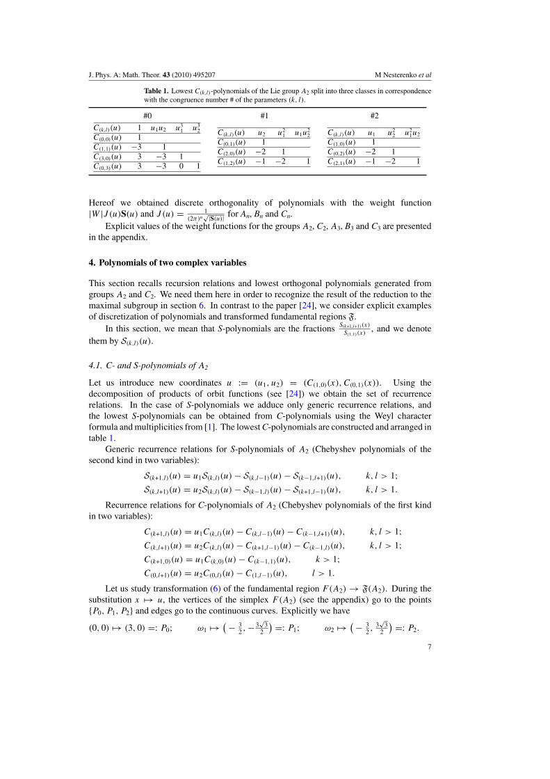
Table 1. Lowest C(k,l)-polynomials of the Lie group A2 split into three classes in correspondencewith the congruence number # of the parameters (k, l).

#0 #1 #2

C(k,l)(u) 1 u1u2 u31 u3

2C(0,0)(u) 1C(1,1)(u) −3 1C(3,0)(u) 3 −3 1C(0,3)(u) 3 −3 0 1

C(k,l)(u) u2 u21 u1u

22

C(0,1)(u) 1C(2,0)(u) −2 1C(1,2)(u) −1 −2 1

C(k,l)(u) u1 u22 u2

1u2

C(1,0)(u) 1C(0,2)(u) −2 1C(2,1)(u) −1 −2 1

Hereof we obtained discrete orthogonality of polynomials with the weight function|W |J (u)S(u) and J (u) = 1

(2π)n√|S(u)| for An, Bn and Cn.

Explicit values of the weight functions for the groups A2, C2, A3, B3 and C3 are presentedin the appendix.

4. Polynomials of two complex variables

This section recalls recursion relations and lowest orthogonal polynomials generated fromgroups A2 and C2. We need them here in order to recognize the result of the reduction to themaximal subgroup in section 6. In contrast to the paper [24], we consider explicit examplesof discretization of polynomials and transformed fundamental regions F.

In this section, we mean that S-polynomials are the fractions S(k+1,l+1)(x)

S(1,1)(x), and we denote

them by S(k,l)(u).

4.1. C- and S-polynomials of A2

Let us introduce new coordinates u := (u1, u2) = (C(1,0)(x), C(0,1)(x)). Using thedecomposition of products of orbit functions (see [24]) we obtain the set of recurrencerelations. In the case of S-polynomials we adduce only generic recurrence relations, andthe lowest S-polynomials can be obtained from C-polynomials using the Weyl characterformula and multiplicities from [1]. The lowest C-polynomials are constructed and arranged intable 1.

Generic recurrence relations for S-polynomials of A2 (Chebyshev polynomials of thesecond kind in two variables):

S(k+1,l)(u) = u1S(k,l)(u) − S(k,l−1)(u) − S(k−1,l+1)(u), k, l > 1;S(k,l+1)(u) = u2S(k,l)(u) − S(k−1,l)(u) − S(k+1,l−1)(u), k, l > 1.

Recurrence relations for C-polynomials of A2 (Chebyshev polynomials of the first kindin two variables):

C(k+1,l)(u) = u1C(k,l)(u) − C(k,l−1)(u) − C(k−1,l+1)(u), k, l > 1;C(k,l+1)(u) = u2C(k,l)(u) − C(k+1,l−1)(u) − C(k−1,l)(u), k, l > 1;C(k+1,0)(u) = u1C(k,0)(u) − C(k−1,1)(u), k > 1;C(0,l+1)(u) = u2C(0,l)(u) − C(1,l−1)(u), l > 1.

Let us study transformation (6) of the fundamental region F(A2) → F(A2). During thesubstitution x → u, the vertices of the simplex F(A2) (see the appendix) go to the points{P0, P1, P2} and edges go to the continuous curves. Explicitly we have

(0, 0) → (3, 0) =: P0; ω1 → ( − 32 ,− 3

√3

2

) =: P1; ω2 → ( − 32 , 3

√3

2

) =: P2.

7

J. Phys. A: Math. Theor. 43 (2010) 495207 M Nesterenko et al

1 1 2 3

2

1

1

2

Figure 1. Region of orthogonality F of polynomials of A2 and discrete points of F3 obtained inexample 2.

Example 2. Let us fix M = 3. |F3(A2)| = 10 and the corresponding grid points ( s1M

, s2M

) incoordinates (Re(u1), Im(u1)) are

(0, 0) → (3, 0); (0, 1) →(

−3

2,

3√

3

2

);

(2

3,

1

3

)→

(−2 cos π

9 + cos2π

9,−2 sin

π

9− sin

2π

9

); (1, 0) →

(−3

2,−3

√3

2

);(

2

3, 0

)→

(− cos

π

9+ 2 sin

π

18,−2 cos

π

18+ sin

π

9

);(

1

3,

2

3

)→

(−2 cos

π

9+ cos

2π

9, 2 sin

π

9+ sin

2π

9

);(

1

3, 0

)→

(2 cos

2π

9+ sin

π

18, cos

π

18− 2 sin

2π

9

);(

0,1

3

)→

(2 cos

2π

9+ sin

π

18,− cos

π

18+ 2 sin

2π

9

);(

1

3,

1

3

)→ (0, 0);

(0,

2

3

)→

(−2 cos

π

9+ 2 sin

π

18, 2 cos

π

18− sin

π

9

).

The choice of new coordinates in the form (Re(u1), Im(u1)) is determined by the complexconjugation u1 = u2. Plotting these points and the transformed fundamental region F infigure 1, we see that the discrete set FM(A2) in new coordinates (u1, u2) goes to pointsFM(A2) ⊂ F(A2).

8

J. Phys. A: Math. Theor. 43 (2010) 495207 M Nesterenko et al

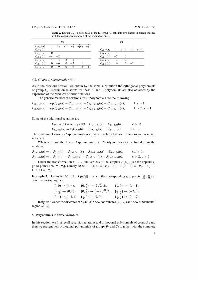
Table 2. Lowest C(k,l)-polynomials of the Lie group C2 split into two classes in correspondencewith the congruence number # of the parameters (k, l).

#0 #1

C(k,l)(u) 1 u2 u21 u2

2 u21u2 u3

2C(0,0)(u) 1C(0,1)(u) 0 1C(2,0)(u) −4 −2 1C(0,2)(u) 4 4 −2 1C(2,1)(u) 0 −6 0 −2 1C(0,3)(u) 0 9 0 6 −3 1

C(k,l)(u) u1 u1u2 u31 u1u

22

C(1,0)(u) 1C(1,1)(u) −2 1C(3,0)(u) −3 −3 1C(1,2)(u) 6 3 −2 1

4.2. C- and S-polynomials of C2

As in the previous section, we obtain by the same substitution the orthogonal polynomialsof group C2. Recursion relations for these S- and C-polynomials are also obtained by theexpansion of the products of orbit functions.

The generic recurrence relations for C-polynomials are the following:

C(k+1,l)(u) = u1C(k,l)(u) − C(k−1,l)(u) − C(k+1,l−1)(u) − C(k−1,l+1)(u), k, l > 1;C(k,l+1)(u) = u2C(k,l)(u) − C(k,l−1)(u) − C(k+2,l−1)(u) − C(k−2,l+1)(u), k > 2, l > 1.

Some of the additional relations are

C(k+1,0)(u) = u1C(k,0)(u) − C(k−1,0)(u) − C(k−1,1)(u), k > 1;C(0,l+1)(u) = u2C(0,l)(u) − C(0,l−1)(u) − C(2,l−1)(u), l > 1.

The remaining low-order C-polynomials necessary to solve all above recursions are presentedin table 2.

When we have the lowest C-polynomials, all S-polynomials can be found from therelations

S(k+1,l)(u) = u1S(k,l)(u) − S(k+1,l−1)(u) − S(k−1,l+1)(u) − S(k−1,l)(u), k, l > 1;S(k,l+1)(u) = u2S(k,l)(u) − S(k,l−1)(u) − S(k+2,l−1)(u) − S(k−2,l+1)(u), k > 2, l > 1.

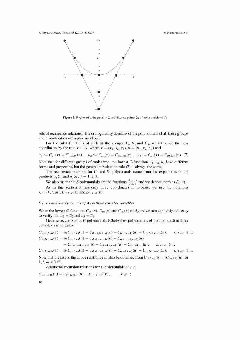
Under the transformation x → u, the vertices of the simplex F(C2) (see the appendix)go to points {P0, P1, P2}, namely (0, 0) → (4, 4) =: P0, ω1 → (0,−4) =: P1, ω2 →(−4, 4) =: P2.

Example 3. Let us fix M = 4. |F4(C2)| = 9 and the corresponding grid points(

s1M

, s2M

)in

coordinates (u1, u2) are

(0, 0) → (4, 4),(0, 1

4

) → (2√

2, 2),(

12 , 0

) → (0,−4),(0, 1

2

) → (0, 0),(0, 3

4

) → ( − 2√

2, 2),

(14 , 1

2

) → (−2, 0),

(0, 1) → (−4, 4),(

14 , 0

) → (2, 0),(

14 , 1

4

) → (0,−2).

In figure 2 we see the discrete set FM(C2) in new coordinates (u1, u2) and new fundamentalregion F(C2).

5. Polynomials in three variables

In this section, we first recall recursion relations and orthogonal polynomials of group A3 andthen we present new orthogonal polynomials of groups B3 and C3 together with the complete

9

J. Phys. A: Math. Theor. 43 (2010) 495207 M Nesterenko et al

4 2 2 4

4

2

2

4

Figure 2. Region of orthogonality F and discrete points F4 of polynomials of C2.

sets of recurrence relations. The orthogonality domains of the polynomials of all these groupsand discretization examples are shown.

For the orbit functions of each of the groups A3, B3 and C3, we introduce the newcoordinates by the rule x → u, where x = (x1, x2, x3), u = (u1, u2, u3) and

u1 := Cω1(x) = C(1,0,0)(x), u2 := Cω2(x) = C(0,1,0)(x), u3 := Cω3(x) = C(0,0,1)(x). (7)

Note that for different groups of rank three, the lowest C-functions u1, u2, u3 have differentforms and properties, but the general substitution rule (7) is always the same.

The recurrence relations for C- and S- polynomials come from the expansions of theproducts ujCλ and ujSλ, j = 1, 2, 3.

We also mean that S-polynomials are the fractions Sλ+ρ(x)

Sρ(x)and we denote them as Sλ(u).

As in this section λ has only three coordinates in ω-basis, we use the notationsλ = (k, l,m), C(k,l,m)(u) and S(k,l,m)(u).

5.1. C- and S-polynomials of A3 in three complex variables

When the lowest C-functions Cω1(x), Cω2(x) and Cω3(x) of A3 are written explicitly, it is easyto verify that u2 = u2 and u3 = u1.

Generic recursions for C-polynomials (Chebyshev polynomials of the first kind) in threecomplex variables are

C(k+1,l,m)(u) = u1C(k,l,m)(u) − C(k−1,l+1,m)(u) − C(k,l,m−1)(u) − C(k,l−1,m+1)(u), k, l,m � 1;C(k,l+1,m)(u) = u2C(k,l,m)(u) − C(k+1,l,m−1)(u) − C(k+1,l−1,m+1)(u)

− C(k−1,l+1,m−1)(u) − C(k−1,l,m+1)(u) − C(k,l−1,m)(u), k, l,m � 1;C(k,l,m+1)(u) = u3C(k,l,m)(u) − C(k+1,l−1,m)(u) − C(k−1,l,m)(u) − C(k,l+1,m−1)(u), k, l,m � 1.

Note that the last of the above relations can also be obtained from C(k,l,m)(u) = C(m,l,k)(u) fork, l,m ∈ Z

�0.

Additional recursion relations for C-polynomials of A3:

C(k+1,0,0)(u) = u1C(k,0,0)(u) − C(k−1,1,0)(u), k � 1;10

J. Phys. A: Math. Theor. 43 (2010) 495207 M Nesterenko et al

Table 3. Lowest C-polynomials of A3 split into four congruence classes # = 0, # = 1, # = 2 and# = 3.

#0 #1C(k,l,m)(u) 1 u1u3 u2

2 u2u23 u2

1u2

C(0,0,0)(u) 1C(1,0,1)(u) −4 1C(0,2,0)(u) 2 −2 1C(0,1,2)(u) 4 −1 −2 1C(2,1,0)(u) 4 −1 −2 0 1

C(k,l,m)(u) u1 u2u3 u33 u2

1u3 u1u22

C(1,0,0)(u) 1C(0,1,1)(u) −3 1C(0,0,3)(u) 3 −3 1C(2,0,1)(u) −1 −2 0 1C(1,2,0)(u) 5 −1 0 −2 1

#2 #3C(k,l,m)(u) u2 u2

3 u21 u1u2u3 u3

2C(0,1,0)(u) 1C(0,0,2)(u) −2 1C(2,0,0)(u) −2 0 1C(1,1,1)(u) 4 −3 −3 1C(0,3,0)(u) −3 3 3 −3 1

C(k,l,m)(u) u3 u1u2 u31 u1u

23 u2

2u3

C(0,0,1)(u) 1C(1,1,0)(u) −3 1C(3,0,0)(u) 3 −3 1C(1,0,2)(u) −1 −2 0 1C(0,2,1)(u) 5 −1 0 −2 1

C(0,k+1,0)(u) = u2C(0,k,0)(u) − C(0,k−1,0)(u) − C(1,k−1,1)(u), k � 1;C(k+1,l,0)(u) = u1C(k,l,0)(u) − C(k,l−1,1)(u) − C(k−1,l+1,0)(u), k, l � 1;C(k,l+1,0)(u) = u2C(k,l,0)(u) − C(k−1,l,1)(u) − C(k,l−1,0)(u) − C(k+1,l−1,1)(u), k, l � 1;C(k+1,0,m)(u) = u1C(k,0,m)(u) − C(k−1,1,m)(u) − C(k,0,m−1)(u), k,m � 1.

The remaining low-order C-polynomials of A3 can be found in table 3.Let us study the transformation of the fundamental region F(A3) → F(A3). During the

substitution x → u the vertices of the simplex F(A3) (see the appendix) go to the points{P0, P1, P2, P3}:

(0, 0, 0) → (4, 6, 0) =: P0, ω1 → (0,−6,−4) =: P1,

ω2 → (−4, 6, 0) =: P2, ω3 → (0,−6, 4) =: P3.

The shape of the region of orthogonality of polynomials of A3 is presented in figure 3.

Example 4. Let us consider discretization with M = 3. |F3(A3)| = 20 and grid points(s1M

, s2M

, s3M

)in new coordinates (Re(u1), u2, Im(u1)) are

(0, 0, 0) → (4, 6, 0), (0, 0, 1) → (0,−6, 4), (0, 1, 0) → (−4, 6, 0),(23 , 0, 1

3

) → (0,−3,−2),(

23 , 1

3 , 0) → ( − 1

2 ,−3,− 3√

32

),

(13 , 0, 2

3

) → (0,−3, 2),(13 , 2

3 , 0) → (− 3

√3

2 , 3,− 12

),

(0, 2

3 , 13

) → (− 3√

32 , 3, 1

2

),

(13 , 0, 0

) → (3√

32 , 3,− 1

2

),(

0, 13 , 0

) → (2, 3, 0),(

13 , 1

3 , 0) → (0, 0,−1),

(13 , 0, 1

3

) → (1, 0, 0),(13 , 1

3 , 13

) → (−1, 0, 0),(

23 , 0, 0

) → (12 ,−3,− 3

√3

2

),

(0, 0, 2

3

) → (12 ,−3, 3

√3

2

),

(1, 0, 0) → (0,−6,−4),(0, 1

3 , 23

) → ( − 12 ,−3, 3

√3

2

),

(0, 0, 1

3

) → (3√

32 , 3, 1

2

),(

0, 13 , 1

3

) → (0, 0, 1),(0, 2

3 , 0) → (−2, 3, 0).

All these points belong to the new fundamental region F(A3).Using the Weyl character formula and multiplicities from [1], we can obtain S-polynomials

(Chebyshev polynomials of the second kind) in u1, u2 and u3. Or, alternately, having the lowestS-polynomials we can construct other polynomials by means of the following recursions:

11

J. Phys. A: Math. Theor. 43 (2010) 495207 M Nesterenko et al

42

02

4

50

5

4

2

0

2

4

Figure 3. Region of orthogonality F and discrete points F3 of polynomials of A3.

S(k+1,l,m)(u) = u1S(k,l,m)(u) − S(k−1,l+1,m)(u) − S(k,l,m−1)(u) − S(k,l−1,m+1)(u), k, l,m � 2;S(k,l+1,m)(u) = u2S(k,l,m)(u) − S(k,l−1,m)(u) − S(k+1,l−1,m+1)(u) − S(k−1,l+1,m−1)(u)

− S(k+1,l,m−1)(u) − S(k−1,l,m+1)(u), k, l,m � 2;S(k,l,m+1)(u) = u3S(k,l,m)(u) − S(k+1,l−1,m)(u) − S(k−1,l,m)(u) − S(k,l+1,m−1)(u), k, l,m � 2.

5.2. C- and S-polynomials of B3 in three real variables

For group B3, our new coordinates u satisfy the relation ui = ui , i = 1, 2, 3.The following generic recursion relations for C-polynomials hold true when k, l,m � 2:

C(k+1,l,m)(u) = u1C(k,l,m)(u) − C(k,l+1,m−2)(u) − C(k,l−1,m+2)(u) − C(k+1,l−1,m)(u)

− C(k−1,l+1,m)(u) − C(k−1,l,m)(u) − C(k−1,l+1,m)(u) − C(k−1,l,m)(u),

C(k,l+1,m)(u) = u2C(k,l,m)(u) − C(k+1,l−1,m+2)(u) − C(k−1,l−1,m+2)(u) − C(k+1,l−2,m+2)(u)

− C(k−1,l,m+2)(u) − C(k−1,l+2,m−2)(u) − C(k+1,l+1,m−2)(u)

− C(k−1,l+1,m−2)(u) − C(k+1,l,m−2)(u) − C(k−2,l+1,m)(u) − C(k+2,l−1,m)(u),

C(k,l,m+1)(u) = u3C(k,l,m)(u) − C(k+1,l−1,m+1)(u) − C(k,l−1,m+1)(u) − C(k−1,l,m+1)(u)

− C(k−1,l+1,m−1)(u) − C(k,l+1,m−1)(u) − C(k+1,l,m−1)(u) − C(k,l,m−1)(u).

Remaining recurrence relations except for the lowest polynomials are listed below:

C(k+1,l,0)(u) = u1C(k,l,0)(u) − C(k−1,l+1,0)(u) − C(k+1,l−1,0)(u) − C(k−1,l,0)(u) − C(k,l−1,2)(u),

C(k,l+1,0)(u) = u2C(k,l,0)(u) − C(k−2,l+1,0)(u) − C(k+2,l−1,0)(u) − C(k−1,l,2)(u) − C(k,l−1,0)(u)

− C(k+1,l−1,2)(u) − C(k−1,l−1,2)(u) − C(k+1,l−2,2)(u),

C(k+1,0,0)(u) = u1C(k,0,0)(u) − C(k−1,1,0)(u) − C(k−1,0,0)(u),

C(0,l+1,0)(u) = u2C(0,l,0)(u) − C(2,l−1,0)(u) − C(0,l−1,0)(u) − C(1,l−1,2)(u) − C(1,l−2,2)(u),

12

J. Phys. A: Math. Theor. 43 (2010) 495207 M Nesterenko et al

Table 4. Lowest C-polynomials of B3 split into two congruence classes # = 0 and # = 1.

#0C(k,l,m)(u) 1 u1 u2 u2

1 u23 u1u2 u1u

23 u3

1 u22 u2u

23 u2

1u2

C(0,0,0)(u) 1C(1,0,0)(u) 0 1C(0,1,0)(u) 0 0 1C(2,0,0)(u) −6 0 −2 1C(0,0,2)(u) −8 −4 −2 0 1C(1,1,0)(u) 24 8 6 0 −3 1C(1,0,2)(u) 0 −8 −2 −4 0 −2 1C(3,0,0)(u) −24 −15 −6 0 3 −3 0 1C(0,2,0)(u) 12 16 8 4 0 4 −2 0 1C(0,1,2)(u) −48 −20 −20 0 6 −6 0 0 −2 1C(2,1,0)(u) 0 8 −6 4 0 2 −1 0 −2 0 1

#1C(k,l,m)(u) u3 u1u3 u2u3 u3

3 u21u3 u1u2u3

C(0,0,1)(u) 1C(1,0,1)(u) −3 1C(0,1,1)(u) 3 −2 1C(0,0,3)(u) −9 −3 −3 1C(2,0,1)(u) −3 −1 −2 0 1C(1,1,1)(u) 30 12 8 −3 −2 1

C(0,0,m+1)(u) = u3C(0,0,m)(u) − C(0,1,m−1)(u) − C(1,0,m−1)(u) − C(0,0,m−1)(u),

C(k+1,0,m)(u) = u1C(k,0,m)(u) − C(k,1,m−2)(u) − C(k−1,1,m)(u),

C(k,0,m+1)(u) = u3C(k,0,m)(u) − C(k−1,0,m+1)(u) − C(k−1,1,m−1)(u) − C(k,1,m−1)(u)

− C(k,0,m−1)(u) − C(k+1,0,m−1)(u),

C(0,l+1,m)(u) = u2C(0,l,m)(u) − C(1,l−1,m+2)(u) − C(1,l−2,m+2)(u) − C(0,l−1,m)(u)

− C(2,l−1,m)(u) − C(1,l+1,m−2)(u) − C(1,l,m−2)(u),

C(0,l,m+1)(u) = u3C(0,l,m)(u) − C(1,l−1,m+1)(u) − C(0,l−1,m+1)(u) − C(0,l+1,m−1)(u)

− C(0,l,m−1)(u) − C(1,l,m−1)(u).

The lowest C-polynomials of B3 were calculated explicitly and arranged in table 4.As in the previous case, we can use the Weyl character formula or generic recurrence

relations for S-polynomials of B3 valid for k, l,m � 2:

S(k+1,l,m)(u) = u1S(k,l,m)(u) − S(k,l+1,m−2)(u) − S(k,l−1,m+2)(u) − S(k+1,l−1,m)(u)

− S(k−1,l+1,m)(u) − S(k−1,l,m)(u) − S(k−1,l+1,m)(u) − S(k−1,l,m)(u),

S(k,l+1,m)(u) = u2S(k,l,m)(u) − S(k+1,l−1,m+2)(u) − S(k−1,l−1,m+2)(u) − S(k+1,l−2,m+2)(u)

− S(k+1,l,m−2)(u) − S(k−2,l+1,m)(u) − S(k−1,l,m+2)(u) − S(k−1,l+2,m−2)(u)

− S(k+1,l+1,m−2)(u) − S(k−1,l+1,m−2)(u) − S(k+2,l−1,m)(u),

S(k,l,m+1)(u) = u3S(k,l,m)(u) − S(k+1,l−1,m+1)(u) − S(k,l−1,m+1)(u) − S(k−1,l,m+1)(u)

− S(k−1,l+1,m−1)(u) − S(k,l+1,m−1)(u) − S(k+1,l,m−1)(u) − S(k,l,m−1)(u).

Substitution of variables x → u transforms vertices of the simplex F(B3) into vertices ofthe orthogonality domain F(B3) = {P0, P1, P2, P3} as follows:

(0, 0, 0) → (6, 12, 8) =: P0, ω1 → (6, 12,−8) =: P1,

13

J. Phys. A: Math. Theor. 43 (2010) 495207 M Nesterenko et al

5

0

5

0

5

10

5

0

5

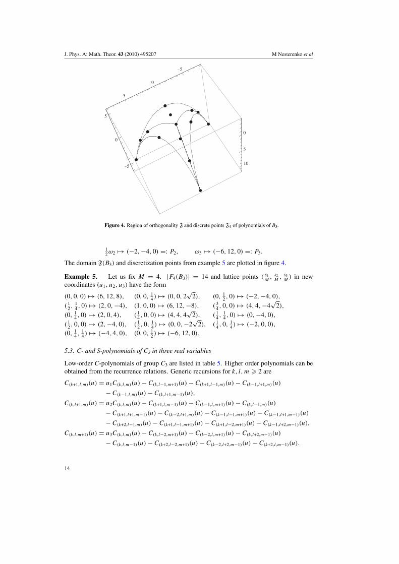
Figure 4. Region of orthogonality F and discrete points F4 of polynomials of B3.

12ω2 → (−2,−4, 0) =: P2, ω3 → (−6, 12, 0) =: P3.

The domain F(B3) and discretization points from example 5 are plotted in figure 4.

Example 5. Let us fix M = 4. |F4(B3)| = 14 and lattice points ( s1M

, s2M

, s3M

) in newcoordinates (u1, u2, u3) have the form

(0, 0, 0) → (6, 12, 8), (0, 0, 14 ) → (0, 0, 2

√2), (0, 1

2 , 0) → (−2,−4, 0),

( 12 , 1

4 , 0) → (2, 0,−4), (1, 0, 0) → (6, 12,−8), ( 34 , 0, 0) → (4, 4,−4

√2),

(0, 14 , 0) → (2, 0, 4), ( 1

4 , 0, 0) → (4, 4, 4√

2), ( 14 , 1

4 , 0) → (0,−4, 0),

( 12 , 0, 0) → (2,−4, 0), ( 1

2 , 0, 14 ) → (0, 0,−2

√2), ( 1

4 , 0, 14 ) → (−2, 0, 0),

(0, 14 , 1

4 ) → (−4, 4, 0), (0, 0, 12 ) → (−6, 12, 0).

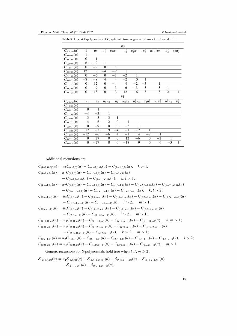
5.3. C- and S-polynomials of C3 in three real variables

Low-order C-polynomials of group C3 are listed in table 5. Higher order polynomials can beobtained from the recurrence relations. Generic recursions for k, l,m � 2 are

C(k+1,l,m)(u) = u1C(k,l,m)(u) − C(k,l−1,m+1)(u) − C(k+1,l−1,m)(u) − C(k−1,l+1,m)(u)

− C(k−1,l,m)(u) − C(k,l+1,m−1)(u),

C(k,l+1,m)(u) = u2C(k,l,m)(u) − C(k+1,l,m−1)(u) − C(k−1,l,m+1)(u) − C(k,l−1,m)(u)

− C(k+1,l+1,m−1)(u) − C(k−2,l+1,m)(u) − C(k−1,l−1,m+1)(u) − C(k−1,l+1,m−1)(u)

− C(k+2,l−1,m)(u) − C(k+1,l−1,m+1)(u) − C(k+1,l−2,m+1)(u) − C(k−1,l+2,m−1)(u),

C(k,l,m+1)(u) = u3C(k,l,m)(u) − C(k,l−2,m+1)(u) − C(k−2,l,m+1)(u) − C(k,l+2,m−1)(u)

− C(k,l,m−1)(u) − C(k+2,l−2,m+1)(u) − C(k−2,l+2,m−1)(u) − C(k+2,l,m−1)(u).

14

J. Phys. A: Math. Theor. 43 (2010) 495207 M Nesterenko et al

Table 5. Lowest C-polynomials of C3 split into two congruence classes # = 0 and # = 1.

#0C(k,l,m)(u) 1 u2 u2

1 u1u3 u22 u2

1u2 u23 u1u2u3 u3

2 u2u23

C(0,0,0)(u) 1C(0,1,0)(u) 0 1C(2,0,0)(u) −6 −2 1C(1,0,1)(u) 0 −2 0 1C(0,2,0)(u) 12 8 −4 −2 1C(2,1,0)(u) 0 −6 0 −1 −2 1C(0,0,2)(u) −8 −8 4 4 −2 0 1C(1,1,1)(u) 0 12 0 −4 4 −2 −3 1C(0,3,0)(u) 0 9 0 3 6 −3 3 −3 1C(0,1,2)(u) 0 −18 0 3 −12 6 3 3 −2 1

#1C(k,l,m)(u) u1 u3 u1u2 u3

1 u2u3 u21u3 u1u

22 u1u

23 u2

2u3 v33

C(1,0,0)(u) 1C(0,0,1)(u) 0 1C(1,1,0)(u) −4 −3 1C(3,0,0)(u) −3 3 −3 1C(0,1,1)(u) 4 6 −2 0 1C(2,0,1)(u) 0 −9 0 0 −2 1C(1,2,0)(u) 12 −3 9 −4 −1 −2 1C(1,0,2)(u) −12 −6 −6 4 −1 4 −2 1C(0,2,1)(u) 0 27 0 0 12 −6 0 −2 1C(0,0,3)(u) 0 −27 0 0 −18 9 0 6 −3 1

Additional recursions are

C(k+1,0,0)(u) = u1C(k,0,0)(u) − C(k−1,1,0)(u) − C(k−1,0,0)(u), k > 1;C(k+1,l,0)(u) = u1C(k,l,0)(u) − C(k,l−1,1)(u) − C(k−1,l,0)(u)

− C(k+1,l−1,0)(u) − C(k−1,l+1,0)(u), k, l > 1;C(k,l+1,0)(u) = u2C(k,l,0)(u) − C(k−1,l,1)(u) − C(k,l−1,0)(u) − C(k+2,l−1,0)(u) − C(k−2,l+1,0)(u)

− C(k−1,l−1,1)(u) − C(k+1,l−1,1)(u) − C(k+1,l−2,1)(u), k, l > 2;C(0,l+1,m)(u) = u2C(0,l,m)(u) − C(1,l,m−1)(u) − C(0,l−1,m)(u) − C(2,l−1,m)(u) − C(1,l+1,m−1)(u)

− C(1,l−1,m+1)(u) − C(1,l−2,m+1)(u), l > 2, m > 1;C(0,l,m+1)(u) = u3C(0,l,m)(u) − C(0,l−2,m+1)(u) − C(0,l,m−1)(u) − C(2,l−2,m+1)(u)

− C(2,l,m−1)(u) − C(0,l+2,m−1)(u), l > 2, m > 1;C(k+1,0,m)(u) = u1C(k,0,m)(u) − C(k−1,1,m)(u) − C(k,1,m−1)(u) − C(k−1,0,m)(u), k,m > 1;C(k,0,m+1)(u) = u3C(k,0,m)(u) − C(k−2,0,m+1)(u) − C(k,0,m−1)(u) − C(k−2,2,m−1)(u)

− C(k+2,0,m−1)(u) − C(k,2,m−1)(u), k > 2, m > 1;C(0,l+1,0)(u) = u2C(0,l,0)(u) − C(0,l−1,0)(u) − C(2,l−1,0)(u) − C(1,l−1,1)(u) − C(1,l−2,1)(u), l > 2;C(0,0,m+1)(u) = u3C(0,0,m)(u) − C(0,0,m−1)(u) − C(2,0,m−1)(u) − C(0,2,m−1)(u), m > 1.

Generic recursions for S-polynomials hold true when k, l,m � 2 :

S(k+1,l,m)(u) = u1S(k,l,m)(u) − S(k,l−1,m+1)(u) − S(k+1,l−1,m)(u) − S(k−1,l+1,m)(u)

− S(k−1,l,m)(u) − S(k,l+1,m−1)(u),

15

J. Phys. A: Math. Theor. 43 (2010) 495207 M Nesterenko et al

50

5

0

5

10

5

0

5

Figure 5. Region of orthogonality F and discrete points F4 of polynomials of C3.

S(k,l+1,m)(u) = u2S(k,l,m)(u) − S(k+1,l,m−1)(u) − S(k−1,l,m+1)(u) − S(k+2,l−1,m)(u)

− S(k−2,l+1,m)(u) − S(k−1,l−1,m+1)(u) − S(k−1,l+1,m−1)(u) − S(k+1,l+1,m−1)(u)

− S(k+1,l−1,m+1)(u) − S(k+1,l−2,m+1)(u) − S(k−1,l+2,m−1)(u) − S(k,l−1,m)(u),

S(k,l,m+1)(u) = u3S(k,l,m)(u) − S(k,l−2,m+1)(u) − S(k−2,l,m+1)(u) − S(k,l+2,m−1)(u)

− S(k+2,l−2,m+1)(u) − S(k−2,l+2,m−1)(u) − S(k+2,l,m−1)(u) − S(k,l,m−1)(u).

Let us study the transformation of the fundamental region F(C3) → F(C3). During thesubstitution x → u, the vertices of the simplex F(C3) (see the appendix) go to the points{P0, P1, P2, P3}:

(0, 0, 0) → (6, 12, 8) =: P0, ω1 → (2,−4,−8) =: P1,

ω2 → (−2,−4, 8) =: P2, ω3 → (−6, 12,−8) =: P3.

The region of orthogonality of polynomials of C3 is presented in figure 5.

Example 6. Let us fix M = 4. |F4(C3)| = 14 and lattice points ( s1M

, s2M

, s3M

) ∈ F4 map to(u1, u2, u3):

(0, 0, 0) → (6, 12, 8),(0, 0, 1

4

) → (3√

2, 6, 2√

2),(0, 1

4 , 0) → (2, 0, 0),(

0, 14 , 1

4

) → (−√

2,−2, 2√

2),(

14 , 0, 1

4

) → (√

2,−2,−2√

2),(14 , 0, 1

2

) → (−2, 0, 0),(14 , 1

4 , 0) → (0,−4, 0),

(0, 1

2 , 0) → (−2,−4, 8),

(0, 1

4 , 12

) → (−4, 4, 0),(12 , 0, 0

) → (2,−4,−8), (0, 0, 1) → (−6, 12,−8),(0, 0, 1

2

) → (0, 0, 0),(14 , 0, 0

) → (4, 4, 0),(0, 0, 3

4

) → (−3√

2, 6,−2√

2).

16

J. Phys. A: Math. Theor. 43 (2010) 495207 M Nesterenko et al

These points are shown on the orthogonality domain F(C3) in figure 5.

6. Branching rules for polynomials of A2, C2, G2, A3, B3 and C3

Complete reducibility (or ‘branching’) of representations of simple Lie groups into thedirect sum of representations of their maximal reductive subgroup translates into completereducibility of the corresponding characters, orbit functions, and their polynomials. In thissection we consider the polynomials of simple Lie groups of rank �3 and their branching intothe sum of polynomials of their maximal semisimple subgroup.

Probably the most interesting class of cases can be identified by the maximal semisimplesubgroups contained in the simple Lie groups. There are the following cases to consider:

A2 ⊃ A1;C2 ⊃ A1 × A1, C2 ⊃ A1;G2 ⊃ A1 × A1, G2 ⊃ A2, G2 ⊃ A1.

A3 ⊃ C2, A3 ⊃ A1 × A1;B3 ⊃ A3, B3 ⊃ A1 × A1 × A1, B3 ⊃ G2;C3 ⊃ C2 × A1, C3 ⊃ A2, C3 ⊃ A1.

In addition, complete reduction of polynomials takes place when the subgroup is non-semisimple reductive. Three such subgroups are maximal with rank �3, namelyA2 ⊃ A1 × U1, A3 ⊃ A2 × U1 and B3 ⊃ B2 × U1. Here, irreducible polynomials ofthe 1-parametric group U1 are trivially all monomials, say Yk, with integer k positive ornegative.

Finally, complete reduction of polynomials happens when the relation between the pairof groups is not inclusion but subjoining [25]. A classification of all such relations is in [21].

6.1. Polynomials of the Lie algebra A1

It was shown in [23, 24] that there is a one-to-one correspondence between C- and S-polynomials of A1 and Chebyshev polynomials of the first and second kind respectively. Herewe just write down the explicit form of the C-polynomials of A1 (the Chebyshev polynomialsof the first kind) traditionally denoted by Tm, m = 0, 1, 2, . . . .

T0(x) = 1, T1(x) = x, T2(x) = 2x2 − 1, T3(x) = 4x3 − 3x,

T4(x) = 8x4 − 8x2 + 1, Tm+1(x) = 2xTm − Tm−1.

The equivalent set of polynomials can be obtained via the substitution x = y

2 , and up to thescaling factor they are

T0(y) = 1, T1(y) = y, T2(y) = y2 − 2,

T3(y) = y3 − 3y, T4(y) = y4 − 4y2 + 2, . . . .

Polynomials Tm are usually called Dickson polynomials and it is well known that them areequivalent to Chebyshev polynomials over the complex numbers. We suppose that in the caseof An Dickson polynomials (as permutation polynomials) act equivalently to the Weyl groupof An in turn equivalent to Sn+1 [23], but this hypothesis requires independent investigation.

6.2. Reductions of polynomials of rank two simple Lie groups

In this section, we present explicit forms of projection matrices Pr providing reductions fromthe rank two simple Lie groups G to their maximal subgroups H. For each set {G ⊃ H, Pr} we

17

J. Phys. A: Math. Theor. 43 (2010) 495207 M Nesterenko et al

obtain the corresponding substitution of variables Xi → fi(Y1, Y2) or Xi → fi(Y ), i = 1, 2that reduces the orthogonal polynomials of G to the polynomials of H. Explicit examples ofC-polynomial reductions are shown for all pairs G ⊃ H .

Here we use the notation of polynomial variables taken from the paper [24], namelyXi := Cωi

, instead of ui = Xi , i = 1, 2 as in previous sections.

Reduction from A2 to A1

Pr = (2 2 );C(1,0)(A2) → C(2)(A1),

C(0,1)(A2) → C(2)(A1); thereforeX1 → Y 2 − 2,

X2 → Y 2 − 2.

Example of reduction: Consider the reduction of a few low-order polynomials of A2. Hereafterthe explicit forms of polynomials of simple Lie groups of rank two are taken from the paper[24].

C(1,1)(A2) = X1X2 − 3 → Y 4 − 4Y 2 + 1 = T4(Y ) − Y ;C(0,2)(A2) = X2

2 − 2X1 → Y 4 − 6Y 2 + 8 = T4(Y ) − 2T2(Y ) + 2.

Reduction from C2 to A1 × A1 =: A(1)1 × A

(2)1

Pr =(

1 10 1

);

C(1,0)(C2) → C(1)

(A

(1)1

)C(0)

(A

(2)1

),

C(0,1)(C2) → C(0)

(A

(1)1

)C(1)

(A

(2)1

); thereforeX1 → Y1,

X2 → Y2.

Example of reduction: in this example, Chebyshev polynomials Tm(Y1), m = 1, 2, . . .

correspond to the Lie group A(1)1 , and Tm(Y2) correspond to group A

(2)1 :

C(2,1)(C2) = X21X2 − 2X2

2 − 6X2 → Y 21 Y2 − 2Y 2

2 − 6Y2 = (T2(Y1) − 4)Y2 − 2(T2(Y2) + 2);C(3,0)(C2) = X3

1 − 3X1X2 − 3X1 → Y 31 − 3Y1Y2 − 3Y1 = T3(Y1) − 3Y1Y2.

Reduction from C2 to A1

Pr = (3 4 );C(1,0)(C2) → C(3)(A1),

C(0,1)(C2) → C(4)(A1); thereforeX1 → Y 3 − 3Y,

X2 → Y 4 − 4Y 2 + 2.

Example of reduction:

C(1,1)(C2) = X1X2 − 2X1 → Y 7 − 7Y 5 + 12Y 3 = T7(Y ) − 2T3(Y ) + Y ;C(0,2)(C2) = X2

1 − 2X1 − 4 → Y 6 − 8Y 4 + 17Y 2 − 8 = T6(Y ) − 2T4(Y ) − 2.

Reduction from G2 to A2:

Pr =(

1 01 1

);

C(1,0)(G2) → C(1,1)(A2),

C(0,1)(G2) → C(0,1)(A2); thereforeX1 → Y1Y2 − 3,

X2 → Y2.

18

J. Phys. A: Math. Theor. 43 (2010) 495207 M Nesterenko et al

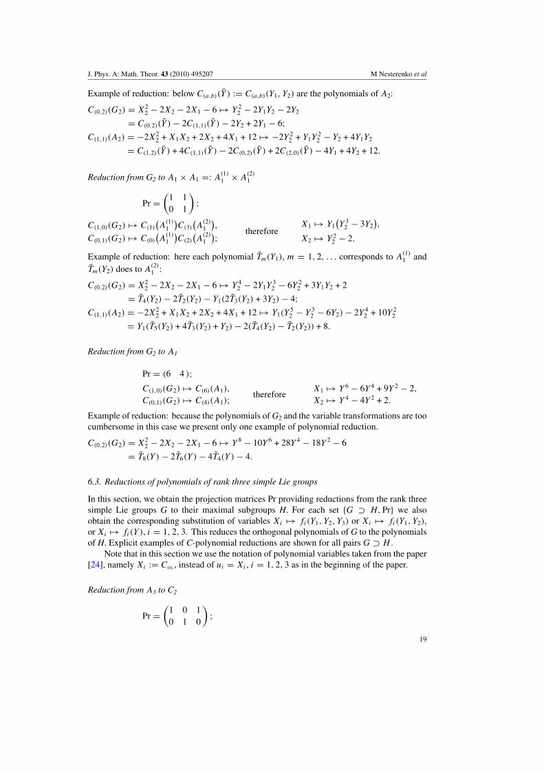
Example of reduction: below C(a,b)(Y ) := C(a,b)(Y1, Y2) are the polynomials of A2:

C(0,2)(G2) = X22 − 2X2 − 2X1 − 6 → Y 2

2 − 2Y1Y2 − 2Y2

= C(0,2)(Y ) − 2C(1,1)(Y ) − 2Y2 + 2Y1 − 6;C(1,1)(A2) = −2X2

2 + X1X2 + 2X2 + 4X1 + 12 → −2Y 22 + Y1Y

22 − Y2 + 4Y1Y2

= C(1,2)(Y ) + 4C(1,1)(Y ) − 2C(0,2)(Y ) + 2C(2,0)(Y ) − 4Y1 + 4Y2 + 12.

Reduction from G2 to A1 × A1 =: A(1)1 × A

(2)1

Pr =(

1 10 1

);

C(1,0)(G2) → C(1)

(A

(1)1

)C(3)

(A

(2)1

),

C(0,1)(G2) → C(0)

(A

(1)1

)C(2)

(A

(2)1

); thereforeX1 → Y1

(Y 3

2 − 3Y2),

X2 → Y 22 − 2.

Example of reduction: here each polynomial Tm(Y1), m = 1, 2, . . . corresponds to A(1)1 and

Tm(Y2) does to A(2)1 :

C(0,2)(G2) = X22 − 2X2 − 2X1 − 6 → Y 4

2 − 2Y1Y32 − 6Y 2

2 + 3Y1Y2 + 2

= T4(Y2) − 2T2(Y2) − Y1(2T3(Y2) + 3Y2) − 4;C(1,1)(A2) = −2X2

2 + X1X2 + 2X2 + 4X1 + 12 → Y1(Y52 − Y 3

2 − 6Y2) − 2Y 42 + 10Y 2

2

= Y1(T5(Y2) + 4T3(Y2) + Y2) − 2(T4(Y2) − T2(Y2)) + 8.

Reduction from G2 to A1

Pr = (6 4 );C(1,0)(G2) → C(6)(A1),

C(0,1)(G2) → C(4)(A1); thereforeX1 → Y 6 − 6Y 4 + 9Y 2 − 2,

X2 → Y 4 − 4Y 2 + 2.

Example of reduction: because the polynomials of G2 and the variable transformations are toocumbersome in this case we present only one example of polynomial reduction.

C(0,2)(G2) = X22 − 2X2 − 2X1 − 6 → Y 8 − 10Y 6 + 28Y 4 − 18Y 2 − 6

= T8(Y ) − 2T6(Y ) − 4T4(Y ) − 4.

6.3. Reductions of polynomials of rank three simple Lie groups

In this section, we obtain the projection matrices Pr providing reductions from the rank threesimple Lie groups G to their maximal subgroups H. For each set {G ⊃ H, Pr} we alsoobtain the corresponding substitution of variables Xi → fi(Y1, Y2, Y3) or Xi → fi(Y1, Y2),or Xi → fi(Y ), i = 1, 2, 3. This reduces the orthogonal polynomials of G to the polynomialsof H. Explicit examples of C-polynomial reductions are shown for all pairs G ⊃ H .

Note that in this section we use the notation of polynomial variables taken from the paper[24], namely Xi := Cωi

, instead of ui = Xi , i = 1, 2, 3 as in the beginning of the paper.

Reduction from A3 to C2

Pr =(

1 0 10 1 0

);

19

J. Phys. A: Math. Theor. 43 (2010) 495207 M Nesterenko et al

C(1,0,0)(A3) → C(1,0)(C2),

C(0,1,0)(A3) → C(0,1)(C2),

C(0,0,1)(A3) → C(1,0)(C2);therefore

X1 → Y1,

X2 → Y2,

X3 → Y1.

Example of reduction: below C(a,b)(Y ) := C(a,b)(Y1, Y2) are the polynomials of the subalgebraC2:

C(1,0,1)(A3) = −4 + X1X3 → −4 + Y 21 = C(2,0)(Y ) + 2Y2;

C(0,1,1)(A3) = −3X1 + X2X3 → −3Y1 + Y1Y2 = C(1,1)(Y ) − Y1.

Reduction from A3 to A1 × A1 =: A(1)1 × A

(2)1

Pr =(

1 0 11 2 1

);

C(1,0,0)(A3) → C1(A

(1)1

)C1(A

(2)1 ),

C(0,1,0)(A3) → C0(A

(1)1

)C2

(A

(2)1

),

C(0,0,1)(A3) → C1(A

(1)1

)C1

(A

(2)1

); thereforeX1 → Y1Y2,

X2 → Y 22 − 2,

X3 → Y1Y2.

Example of reduction: in this example, Chebyshev polynomials Tm(Yi), m = 1, 2, . . .

correspond to the Lie group A(i)1 , i = 1, 2.

C(1,0,1) = −4 + X1X3 → −4 + Y 21 Y 2

2 = T2(Y1)T2(Y2) + 2T2(Y1) + 2T2(Y2);C(0,1,1) = −3X1 + X2X3 → −5Y1Y2 + Y1Y

32 = Y1T3(Y2) − 2Y1Y2.

Reduction from B3 to A3

Pr =⎛⎝0 1 1

1 1 00 1 0

⎞⎠ ;

C(1,0,0)(B3) → C(0,1,0)(A3),

C(0,1,0)(B3) → C(1,1,1)(A3),

C(0,0,1)(B3) → C(1,0,0)(A3);therefore

X1 → Y2,

X2 → Y1Y2Y3 − 3Y 21 − 3Y 2

3 + 4Y2,

X3 → Y1.

Example of reduction: below C(a,b,c)(Y ) := C(a,b,c)(Y1, Y2, Y3) are polynomials of thesubalgebra A3:

C(1,0,1)(B3) = X1X3 − 3X3 → Y1Y2 − 3Y1 = C(1,1,0)(Y ) − 3Y1 + 3Y3;C(0,0,2)(B3) = X2

3 − 2X2 − 4X1 − 8 → 6Y 23 − 2Y1Y2Y3 − 12Y2 + 7Y 2

1 − 8

= −2C(1,1,1)(Y ) + C(2,0,0)(Y ) − 2Y2 − 8.

Reduction from B3 to 3A1 =: A(1)1 × A

(2)1 × A

(3)1

Pr =⎛⎝1 1 0

1 1 10 2 1

⎞⎠ ;

C(1,0,0)(B3) → C1(A1

1

)C1

(A2

1

)C0

(A3

1

),

C(0,1,0)(B3) → C1(A1

1

)C1

(A2

1

)C2

(A3

1

),

C(0,0,1)(B3) → C0(A1

1

)C1

(A2

1

)C1

(A3

1

); thereforeX1 → Y1Y2,

X2 → Y1Y2(Y 2

3 − 2),

X3 → Y2Y3.

20

J. Phys. A: Math. Theor. 43 (2010) 495207 M Nesterenko et al

Example of reduction: the variables refer to the three different subalgebras A1. The Chebyshevpolynomials Tm(Yi), m = 1, 2, . . . correspond to the Lie group A

(i)1 , i = 1, 2, 3.

C(1,0,1)(B3) = X1X3 − 3X3 → Y1Y22 Y3 − 3Y2Y3 = Y1T2(Y2)Y3 + 2Y1Y3 − 3Y2Y3;

C(0,1,1)(B3) = X2X3 − 2X1X3 + 3X3 → Y1Y22 Y 3

3 − 4Y1Y22 Y3 + 3Y2Y3

= Y1T2(Y2)T3(Y3) − Y1T2(Y2)Y3 + 2Y1T3(Y3) − 2Y1Y3 + 3Y2Y3.

Reduction from B3 to G2

Pr =(

0 1 01 0 1

);

C(1,0,0)(B3) → C(0,1)(G2),

C(0,1,0)(B3) → C(1,0)(G2),

C(0,0,1)(B3) → C(0,1)(G2);therefore

X1 → Y2,

X2 → Y1,

X3 → Y2.

Example of reduction: in this example, C(a,b,c)(Y ) := C(a,b)(Y1, Y2) are the polynomials ofsubalgebra G2:

C(1,0,1)(B3) = X1X3 − 3X3 → Y 22 − 3Y2 = C(0,2)(Y ) − Y2 + 2Y1 + 6;

C(1,1,0)(B3) = X21 − 2X2 − 6 → Y 2

2 − 2Y1 − 4Y2 − 8 = C(0,2)(Y ) + Y2.

Reduction from C3 to C2 × A1

Pr =⎛⎝1 0 0

0 1 10 0 1

⎞⎠ ;

C(1,0,0)(C3) → C(1,0)(G2)C0(A1),

C(0,1,0)(C3) → C(0,1)(G2)C0(A1),

C(0,0,1)(C3) → C(0,1)(G2)C1(A1);therefore

X1 → Y1,

X2 → Y2,

X3 → Y2Y3.

Example of reduction: let C(a,b,c)(Y ) := C(a,b)(Y1, Y2) be the polynomials of the subalgebraC2, and Chebyshev polynomials Tm(Y3), m = 1, 2, . . . correspond to the Lie group A1 :

C(1,0,1)(C3) = X1X3 − 2X2 → Y1Y2Y3 − 2Y2 = C(1,1)(Y )Y3 + 2Y1Y3 − 2Y2;C(2,0,0)(C3) = X2

1 − 2X2 − 6 → Y 21 − 2Y2 − 6 = C(2,0)(Y ) − 2.

Reduction from C3 to A2

Pr =(

1 1 20 1 0

);

C(1,0,0)(C3) → C(1,0)(A2),

C(0,1,0)(C3) → C(1,1)(A2),

C(0,0,1)(C3) → C(2,0)(A2);therefore

X1 → Y1,

X2 → Y1Y2 − 3,

X3 → Y 21 − 2Y2.

Example of reduction: in this case, C(a,b,c)(Y ) := C(a,b)(Y1, Y2) are polynomials of thesubalgebra A2:

C(1,0,1)(C3) = X1X3 − 2X2 → Y 31 − 4Y1Y2 + 6 = C(3,0)(Y ) − C(1,1)(Y );

C(2,0,0)(C3) = X21 − 2X2 − 6 → Y 2

1 − 2Y1Y2 + 6 = C(2,0)(Y ) − 2C(1,1)(Y ) + 2Y2.

21

J. Phys. A: Math. Theor. 43 (2010) 495207 M Nesterenko et al

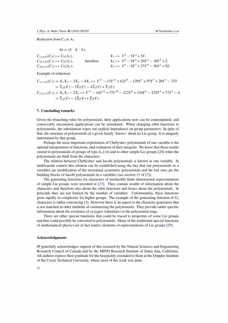
Reduction from C3 to A1

Pr = (5 8 9 );C(1,0,0)(C3) → C5(A1),

C(0,1,0)(C3) → C8(A1),

C(0,0,1)(C3) → C9(A1);therefore

X1 → Y 5 − 5Y 3 + 5Y,

X2 → Y 8 − 8Y 6 + 20Y 4 − 16Y 2 + 2,

X3 → Y 9 − 9Y 7 + 27Y 5 − 30Y 3 + 9Y.

Example of reduction:

C(1,1,0)(C3) = X1X2 − 3X3 − 4X1 → Y 13 − 13Y 11 + 62Y 9 − 129Y 7 + 97Y 5 + 20Y 3 − 37Y

= T13(Y ) − 3T9(Y ) − 4T5(Y ) + T3(Y );C(1,0,1)(C3) = X1X3 − 2X2 → Y 14 − 14Y 12 + 77Y 10 − 212Y 8 + 310Y 6 − 235Y 4 + 77Y 2 − 4

= T14(Y ) − 2T8(Y ) + T4(Y ).

7. Concluding remarks

Given the branching rules for polynomials, their applications now can be contemplated, andconceivably uncommon applications can be stimulated. When changing orbit functions topolynomials, the substitution wipes out explicit dependence on group parameters. In spite ofthat, the structure of polynomials of a given family ‘knows’ about its Lie group. It is uniquelydetermined by that group.

Perhaps the most important exploitation of Chebyshev polynomials of one variable is theoptimal interpolation of functions, and evaluation of their integrals. We know that these resultsextend to polynomials of groups of type An [14] and to other simple Lie groups [20] when thepolynomials are built from the characters.

The relation between Chebyshev and Jacobi polynomials is known in one variable. Inmultivariate context this relation can be established using the fact that our polynomials in nvariables are modification of the monomial symmetric polynomials and the last ones are thebuilding blocks of Jacobi polynomials in n variables (see section 11 of [7]).

The generating functions for characters of irreducible finite dimensional representationsof simple Lie groups were invented in [27]. They contain wealth of information about thecharacters and therefore also about the orbit functions and hence about the polynomials. Inprinciple they are not limited by the number of variables. Unfortunately, these functionsgrow rapidly in complexity for higher groups. The example of the generating function of G2

characters is rather convincing [3]. However there is an aspect to the character generators thatis not matched in other methods of constructing the polynomials. They provide rather specificinformation about the existence of syzygies (identities) in the polynomial rings.

There are other special functions that could be traced to properties of some Lie groupsand that could possibly be converted to polynomials. Many of the traditional special functionsof mathematical physics are in fact matrix elements of representations of Lie groups [29].

Acknowledgments

JP gratefully acknowledges support of this research by the Natural Sciences and EngineeringResearch Council of Canada and by the MIND Research Institute of Santa Ana, California.All authors express their gratitude for the hospitality extended to them at the Doppler Instituteof the Czech Technical University, where most of the work was done.

22

J. Phys. A: Math. Theor. 43 (2010) 495207 M Nesterenko et al

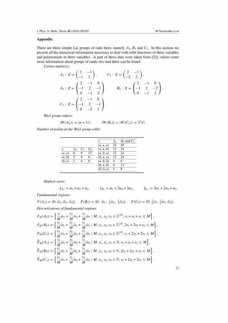
Appendix

There are three simple Lie groups of rank three, namely A3, B3 and C3. In this section wepresent all the numerical information necessary to deal with orbit functions of three variablesand polynomials in three variables. A part of these data were taken from [22], where somemore information about groups of ranks two and three can be found.

Cartan matrices:

A2 : C =(

2 −1−1 2

), C2 : C =

(2 −1

−2 2

),

A3 : C =⎛⎝ 2 −1 0

−1 2 −10 −1 2

⎞⎠ , B3 : C =⎛⎝ 2 −1 0

−1 2 −20 −1 2

⎞⎠ ,

C3 : C =⎛⎝ 2 −1 0

−1 2 −10 −2 2

⎞⎠ .

Weyl group orders:

|W(An)| = (n + 1)!, |W(Bn)| = |W(Cn)| = 2nn!.

Number of points in the Weyl group orbit:

λ A2 C2 G2

(�, �) 6 8 12(�, 0) 3 4 6(0, �) 3 4 6

λ A3 B3 and C3

(�, �, �) 24 48(�, �, 0) 12 24(�, 0, �) 12 24(0, �, �) 12 24(�, 0, 0) 4 6(0, �, 0) 6 12(0, 0, �) 4 8

Highest roots:

ξA3 = α1 + α2 + α3, ξB3 = α1 + 2α2 + 2α3, ξC3 = 2α1 + 2α2 + α3.

Fundamental regions:

F(A3) = {0, ω1, ω2, ω3}, F (B3) = {0, ω1,12 ω2,

12 ω3}, F (C3) = {0, 1

2 ω1,12 ω2, ω3}.

Discretizations of fundamental regions:

FM(A3) ={ s1

Mω1 +

s2

Mω2 +

s3

Mω3 | M, s1, s2, s3 ∈ Z

�0, s1 + s2 + s3 � M}

,

FM(B3) ={ s1

Mω1 +

s2

Mω2 +

s3

Mω3 | M, s1, s2, s3 ∈ Z

�0, 2s1 + 2s2 + s3 � M}

,

FM(C3) ={ s1

Mω1 +

s2

Mω2 +

s3

Mω3 | M, s1, s2, s3 ∈ Z

�0, s1 + 2s2 + 2s3 � M}

.

FM(A3) ={ s1

Mω1 +

s2

Mω2 +

s3

Mω3 | M, s1, s2, s3 ∈ N, s1 + s2 + s3 � M

},

FM(B3) ={ s1

Mω1 +

s2

Mω2 +

s3

Mω3 | M, s1, s2, s3 ∈ N, 2s1 + 2s2 + s3 � M

},

FM(C3) ={ s1

Mω1 +

s2

Mω2 +

s3

Mω3 | M, s1, s2, s3 ∈ N, s1 + 2s2 + 2s3 � M

}.

23

J. Phys. A: Math. Theor. 43 (2010) 495207 M Nesterenko et al

(a, b)

r1 r2

(−a, a+b) (a+b, −b)

(a, b)

r1 r2

(−a, a+b)

r2

(a+2b, −b)

r1

(a+2b, −a−b) (−a−2b, a+b)

W(a,b)(A2) W(a,b)(C2)

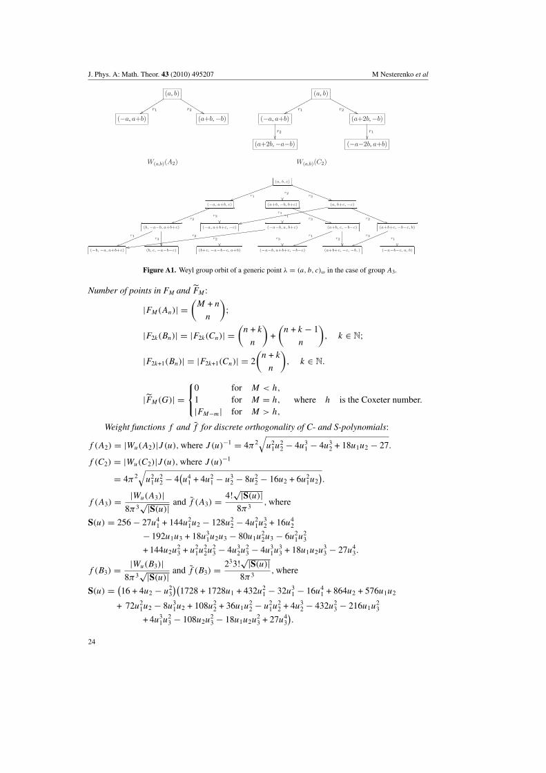
Figure A1. Weyl group orbit of a generic point λ = (a, b, c)ω in the case of group A3.

Number of points in FM and FM :

|FM(An)| =(

M + n

n

);

|F2k(Bn)| = |F2k(Cn)| =(

n + k

n

)+

(n + k − 1

n

), k ∈ N;

|F2k+1(Bn)| = |F2k+1(Cn)| = 2

(n + k

n

), k ∈ N.

|FM(G)| =⎧⎨⎩

0 for M < h,

1 for M = h,

|FM−m| for M > h,

where h is the Coxeter number.

Weight functions f and f for discrete orthogonality of C- and S-polynomials:

f (A2) = |Wu(A2)|J (u), where J (u)−1 = 4π2√

u21u

22 − 4u3

1 − 4u32 + 18u1u2 − 27.

f (C2) = |Wu(C2)|J (u), where J (u)−1

= 4π2√

u21u

22 − 4

(u4

1 + 4u21 − u3

2 − 8u22 − 16u2 + 6u2

1u2).

f (A3) = |Wu(A3)|8π3

√|S(u)| and f (A3) = 4!√|S(u)|8π3

, where

S(u) = 256 − 27u41 + 144u2

1u2 − 128u22 − 4u2

1u32 + 16u4

2

− 192u1u3 + 18u31u2u3 − 80u1u

22u3 − 6u2

1u23

+ 144u2u23 + u2

1u22u

23 − 4u3

2u23 − 4u3

1u33 + 18u1u2u

33 − 27u4

3.

f (B3) = |Wu(B3)|8π3

√|S(u)| and f (B3) = 233!√|S(u)|8π3

, where

S(u) = (16 + 4u2 − u2

3

)(1728 + 1728u1 + 432u2

1 − 32u31 − 16u4

1 + 864u2 + 576u1u2

+ 72u21u2 − 8u3

1u2 + 108u22 + 36u1u

22 − u2

1u22 + 4u3

2 − 432u23 − 216u1u

23

+ 4u31u

23 − 108u2u

23 − 18u1u2u

23 + 27u4

3

).

24

J.Phys.A:M

ath.Theor.43

(2010)495207

MN

esterenkoetal

(a)

(b)

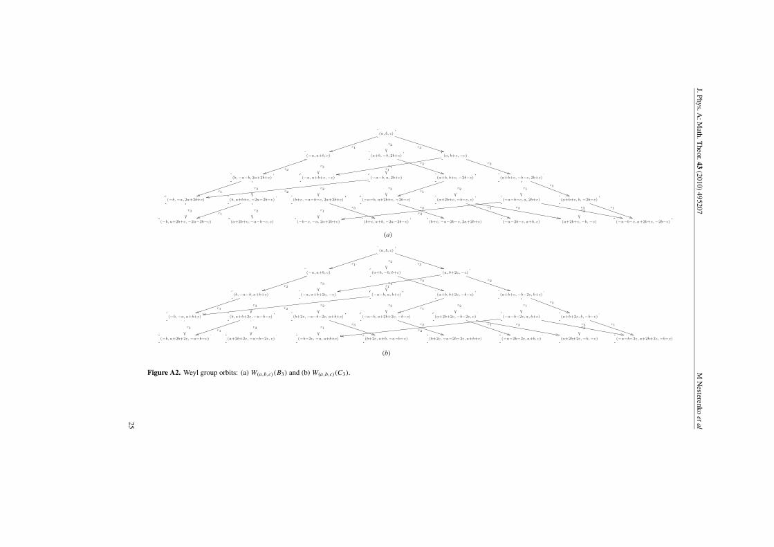
Figure A2. Weyl group orbits: (a) W(a,b,c)(B3) and (b) W(a,b,c)(C3).

25

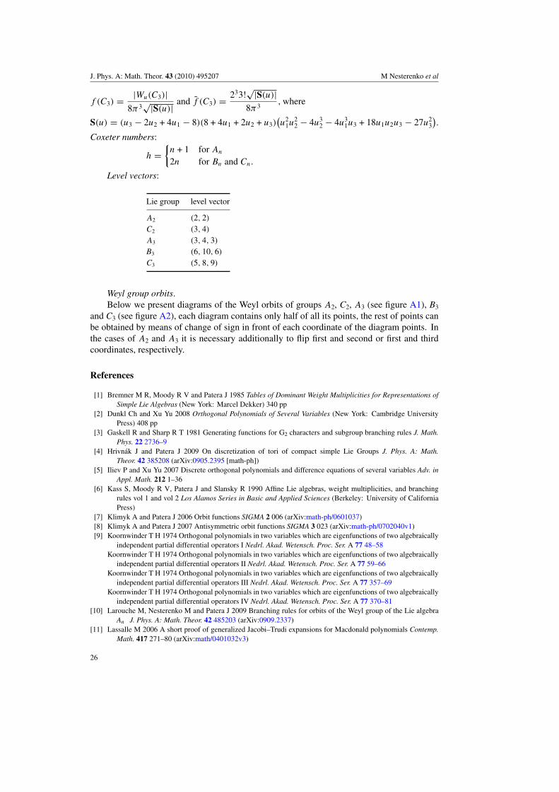
J. Phys. A: Math. Theor. 43 (2010) 495207 M Nesterenko et al

f (C3) = |Wu(C3)|8π3

√|S(u)| and f (C3) = 233!√|S(u)|8π3

, where

S(u) = (u3 − 2u2 + 4u1 − 8)(8 + 4u1 + 2u2 + u3)(u2

1u22 − 4u3

2 − 4u31u3 + 18u1u2u3 − 27u2

3

).

Coxeter numbers:

h ={n + 1 for An

2n for Bn and Cn.

Level vectors:

Lie group level vector

A2 (2, 2)

C2 (3, 4)

A3 (3, 4, 3)

B3 (6, 10, 6)

C3 (5, 8, 9)

Weyl group orbits.Below we present diagrams of the Weyl orbits of groups A2, C2, A3 (see figure A1), B3

and C3 (see figure A2), each diagram contains only half of all its points, the rest of points canbe obtained by means of change of sign in front of each coordinate of the diagram points. Inthe cases of A2 and A3 it is necessary additionally to flip first and second or first and thirdcoordinates, respectively.

References

[1] Bremner M R, Moody R V and Patera J 1985 Tables of Dominant Weight Multiplicities for Representations ofSimple Lie Algebras (New York: Marcel Dekker) 340 pp

[2] Dunkl Ch and Xu Yu 2008 Orthogonal Polynomials of Several Variables (New York: Cambridge UniversityPress) 408 pp

[3] Gaskell R and Sharp R T 1981 Generating functions for G2 characters and subgroup branching rules J. Math.Phys. 22 2736–9

[4] Hrivnak J and Patera J 2009 On discretization of tori of compact simple Lie Groups J. Phys. A: Math.Theor. 42 385208 (arXiv:0905.2395 [math-ph])

[5] Iliev P and Xu Yu 2007 Discrete orthogonal polynomials and difference equations of several variables Adv. inAppl. Math. 212 1–36

[6] Kass S, Moody R V, Patera J and Slansky R 1990 Affine Lie algebras, weight multiplicities, and branchingrules vol 1 and vol 2 Los Alamos Series in Basic and Applied Sciences (Berkeley: University of CaliforniaPress)

[7] Klimyk A and Patera J 2006 Orbit functions SIGMA 2 006 (arXiv:math-ph/0601037)[8] Klimyk A and Patera J 2007 Antisymmetric orbit functions SIGMA 3 023 (arXiv:math-ph/0702040v1)[9] Koornwinder T H 1974 Orthogonal polynomials in two variables which are eigenfunctions of two algebraically

independent partial differential operators I Nedrl. Akad. Wetensch. Proc. Ser. A 77 48–58Koornwinder T H 1974 Orthogonal polynomials in two variables which are eigenfunctions of two algebraically

independent partial differential operators II Nedrl. Akad. Wetensch. Proc. Ser. A 77 59–66Koornwinder T H 1974 Orthogonal polynomials in two variables which are eigenfunctions of two algebraically

independent partial differential operators III Nedrl. Akad. Wetensch. Proc. Ser. A 77 357–69Koornwinder T H 1974 Orthogonal polynomials in two variables which are eigenfunctions of two algebraically

independent partial differential operators IV Nedrl. Akad. Wetensch. Proc. Ser. A 77 370–81[10] Larouche M, Nesterenko M and Patera J 2009 Branching rules for orbits of the Weyl group of the Lie algebra

An J. Phys. A: Math. Theor. 42 485203 (arXiv:0909.2337)[11] Lassalle M 2006 A short proof of generalized Jacobi–Trudi expansions for Macdonald polynomials Contemp.

Math. 417 271–80 (arXiv:math/0401032v3)

26

J. Phys. A: Math. Theor. 43 (2010) 495207 M Nesterenko et al

[12] Lassalle M and Schlosser M J 2006 Inversion of the Pieri formula for Macdonald polynomials Adv.Math. 202 289–325 (arXiv:math/0402127v1)

[13] Lassalle M and Schlosser M J 2010 Recurrence formulas for Macdonald polynomials of type A J. Algebr.Comb. 32 113–31 (arXiv:0902.2099v2)

[14] Li H and Xu Yu 2008 Discrete Fourier analysis on fundamental domain of An lattice and on simplex in d-variablesarXiv:0809.1079

[15] Macdonald I G 1982 Some conjectures for root systems SIAM J. Math. Anal. 13 988–1007[16] Macdonald I G 2000 Orthogonal polynomials associated with root systems Seminaire Lotharingien de

Combinatoire 45 B45a[17] McKay W G and Patera J 1981 Tables of dimensions, indices, and branching rules for representations of simple

Lie algebras (New York: Marcel Dekker) 317 pp[18] Moody R V and Patera J 1987 Computation of character decompositions of class functions on compact

semisimple Lie groups Math. Comput. 48 799–827[19] Moody R V and Patera J 2005 Orthogonality within the families of C-, S- and E-functions of any compact

semisimple Lie group SIGMA 2 076 14 pp (arXiv:math-ph/0512029)[20] Moody R V and Patera J 2010 Cubature formulae for orthogonal polynomials in terms of elements of finite

order of compact simple Lie groups Adv. Appl. Math. at press (arXiv:1005.2773v1)[21] Moody R V and Pianzola A 1983 λ-mappings between the representation rings of Lie algebras Can. J. Math.

35 898–960[22] Nesterenko M and Patera J 2008 Three dimensional C-, S- and E-transforms J. Phys. A: Math. Theor. 41 475205

(arXiv:0805.3731v1)[23] Nesterenko M, Patera J and Tereszkiewicz A 2009 Orbit functions of SU(n) and Chebyshev polynomials

arXiv:0905.2925v2[24] Nesterenko M, Patera J and Tereszkiewicz A 2010 Orthogonal polynomials of compact simple Lie groups

arXiv:1001.3683v2[25] Patera J, Sharp R T and Slansky R 1980 On a new relation between semisimple Lie algebras J. Math.

Phys. 21 2335–41[26] Patera J 2005 Compact simple Lie groups and theirs C-, S-, and E-transforms SIGMA 1 025

(arXiv:math-ph/0512029)[27] Patera J and Sharp R T 1977 Generating functions for characters of group representations and their applications

Group Theoretical Methods in Physics (Springer Lecture Notes in Physics vol 79) p 175–83[28] Rivlin T J 1974 The Chebyshef Polynomials (New York: Wiley)[29] Ja Vilenkin N and Klimyk A U 1995 Representations of Lie Groups and Special Functions: Recent Advances

(Kluwer: Dordrecht)[30] Xu Yu 2004 On discrete orthogonal polynomials of several variables Adv. Appl. Math. 33 615–32

27