
ORTHOGONAL FREQUENCY DIVISION M (OFDM) TRANSCEIVER DESIGN
90
1 ORTHOGONAL FREQUENCY DIVISION MULTIPLEXING (OFDM) TRANSCEIVER DESIGN A DESIGN PROJECT REPORT PRESENTED TO THE ENGINEERING DIVISION OF THE GRADUATE SCHOOL OF CORNELL UNIVERSITY IN PARTIAL FULFILLMENT OF THE REQUIREMENTS FOR THE DEGREE OF MASTER OF ENGINEERING (ELECTRICAL) by Michal Litwin Project Advisor: Bruce R. Land Degree Date: August 2010
Transcript of ORTHOGONAL FREQUENCY DIVISION M (OFDM) TRANSCEIVER DESIGN
1
ORTHOGONAL FREQUENCY DIVISION MULTIPLEXING (OFDM)
TRANSCEIVER DESIGN
A DESIGN PROJECT REPORT
PRESENTED TO THE ENGINEERING DIVISION OF THE GRADUATE SCHOOL
OF CORNELL UNIVERSITY
IN PARTIAL FULFILLMENT OF THE REQUIREMENTS FOR THE DEGREE OF
MASTER OF ENGINEERING (ELECTRICAL)
by
Michal Litwin
Project Advisor: Bruce R. Land
Degree Date: August 2010

2
Abstract
Master of Electrical Engineering Program
Cornell University
Design Project Report
Project Title: Orthogonal Frequency Division Multiplexing (OFDM) Transceiver
Author: Michal Litwin
Abstract:
This project implements an Orthogonal Frequency Division Multiplexing (OFDM)
transceiver in a hybrid Simulink/Verilog programming environment with timing and hardware
resources consideration for an FPGA platform - Altera Cyclone II. The deliverable of the project is
real-time processing MATLAB Simulink model of an OFDM transceiver with the core components
implemented in hardware using hardware descriptive language Verilog.
My choice of the OFDM transceiver design project is motivated by the relevance of its
realization for students who share interest in the communication field. The project provides
opportunity to study outside the classroom a real-time processing software/hardware
implementation of a complete digital communication system based on most commonly used in
wireless technology modulation scheme - Orthogonal Frequency Division Multiplexing.
The orthogonality between overlapping subcarriers which is at the core of OFDM
modulation requires a perfect synchronization. As a consequence, a more sophisticated
synchronization mechanism than in the case of a single carrier modulation necessitates
employment of fast implementations of various commonly used in a receiver design algorithms,
such as CORDIC and Fast-Fourier Transform, which can be re-used in different transceiver’s
architectures.
Report Approved by
Project Advisor: ______________________________________Date: _____________________

3
EXECUTIVE SUMMARY
This project involved design and development of an Orthogonal Frequency Division
Multiplexing transceiver (OFDM) in a hybrid Simulink and Modelsim/Quartus environment for an
FPGA platform - Altera Cyclone II. Orthogonal Frequency Division Multiplexing is the most
commonly used multicarrier modulation scheme in wireless communication due to its robustness
in frequency-selective channels. Advantages of Orthogonal Frequency Division Multiplexing, such as
efficient spectrum utilization due to overlapping subcarriers, stem from the orthogonality principle
between subcarriers which requires perfect timing and frequency synchronization. As a
consequence, the main emphasis in the project was put on design and development of the
synchronization mechanism.
The goal set forth for the project - development of a base software/hardware digital
communication system, which can serve the purpose of an educational tool to supplement students'
coursework in communication theory, is reflected in the aforementioned selection of the project ‘s
technology and associated with it requirements.
Due to the fact that OFDM is an underlying technology of most modern wireless communication
systems one can use and expand the project to study not only the OFDM system but also other
wireless communication features. I developed synchronization mechanism based on a single master
control counter and a state machine which can easily be expanded:
to a larger number of OFDM subcarriers by adjusting a reference of the control signals to
new master control counter values
to include an additional feature by introducing an additional state in the state machine
Development of synchronization mechanism involved implementation of algorithms which are
commonly used in a digital transceiver design, such as:
CORDIC algorithm of linear and circular type in both rotation and vectoring modes
Fast-Fourier Transform
Quadrature digital synthesis without ROM look-up tables
I researched most-up-to-date hardware optimizations of the aforementioned algorithms and
selected representatives which had the highest speed-to-hardware cost ratio. The implementation
was done both in software (MATLAB) and hardware (Verilog HDL). I implemented a fast variation
of CORDIC algorithm in rotation mode which eliminates a critical path from the rotation direction
evaluation with a little hardware cost overhead - a major speed bottleneck in a standard form of
CORDIC algorithm. My implementation of CORDIC algorithm in vectoring mode halves the number
of iterations required for convergence by employing radix-4 modification to the standard CORDIC
algorithm. I designed 64-point multiplierless Fast Fourier Transform unit which in standard
implementation requires 49 nontrivial complex multiplications (49*4 real multipliers). The Fast-
Fourier Transform implementation also offers an outstanding speed performance (14 clock cycles
in a serial output mode and 21 clock cycles in a parallel output mode). The OFDM transceiver is
robust to synchronization errors and achieves error-free decoding in both ideal and moderate
multipath channel conditions.

4
CONTENTS
1 Design problem and system of requirements ..................................................................................... 6
2 Introduction .......................................................................................................................................... 7
2.1 Multicarrier modulation .............................................................................................................. 7
2.2 Orthogonal Frequency Division Multiplexing (OFDM) ................................................................ 7
2.2.1 Advantages of Orthogonal Frequency Division Multiplexing (OFDM) ............................... 7
2.2.2 OFDM modulation ................................................................................................................ 8
2.2.3 OFDM demodulation ............................................................................................................ 8
2.2.4 Guard interval ....................................................................................................................... 9
2.3 System architecture ..................................................................................................................... 9
2.3.1 Description of the OFDM Transceiver’s components ......................................................... 9
3 Algorithms used in the OFDM transceiver’s design .......................................................................... 12
3.1 Fast-Fourier Transform............................................................................................................... 12
3.1.1 Alternative solutions and design choice ............................................................................ 12
3.1.2 Algorithm description ........................................................................................................ 14
3.1.3 Hardware Implementation ................................................................................................ 15
3.1.3.5 Inverse Fast Fourier Transform .......................................................................................... 19
3.2 CORDIC ALGORITHM ................................................................................................................. 19
3.2.1 Introduction ........................................................................................................................ 19
3.2.2 CORDIC algorithm in vectoring mode (circular type) ........................................................ 20
3.2.3 CORDIC algorithm in vectoring mode (linear type) ........................................................... 28
3.2.4 CORDIC algorithm in rotation mode (PARA-CORDIC) ....................................................... 30
4 Synchronization Mechanism – OFDM Receiver Design .................................................................... 37
4.1 Synchronization errors ............................................................................................................... 37
4.1.1 Carrier frequency offset ..................................................................................................... 37
4.1.2 Symbol timing offset .......................................................................................................... 38
4.2 Synchronization schemes ........................................................................................................... 39
4.2.1 Timing Offset Estimation .................................................................................................... 39
4.2.2 Fractional Frequency Offset Estimation ............................................................................ 41
4.2.3 Channel estimation ............................................................................................................ 41

5
4.3 Alternative Solutions And Design Choice .................................................................................. 42
4.4 Hardware implementation ........................................................................................................ 44
4.4.1 Overall architecture............................................................................................................ 44
4.4.2 Coarse Synchronization ...................................................................................................... 46
4.4.3 Fine synchronization .......................................................................................................... 52
4.4.4 Channel Estimation ............................................................................................................ 54
4.4.5 Data decoding ..................................................................................................................... 55
5 Testing................................................................................................................................................. 56
6 Results ................................................................................................................................................. 57
6.1 Results for assessment of reusability of the hardware implementation of the algorithms
used in the OFDM transceiver’s design ................................................................................................. 57
6.2 Results for assessment of reusability of the OFDM transceiver ............................................... 64
7 Conclusion .......................................................................................................................................... 67
References .............................................................................................................................................. 68
8 Appendix ............................................................................................................................................. 70
8.1 Circuit diagrams .......................................................................................................................... 70
8.2 Testing results............................................................................................................................. 75
8.2.1 Ideal channel ...................................................................................................................... 75
8.2.2 Mild multi-path channel..................................................................................................... 77
8.2.3 Severe multi-path channel ................................................................................................. 80
8.2.4 Ideal channel with an uncompensated frequency offset ................................................. 82
8.2.5 Ideal channel with a symbol timing offset (FFT window leads) ....................................... 84
8.2.6 Ideal channel with a symbol timing offset (FFT window lags) .......................................... 86
8.2.7 Ideal channel with both a symbol timing offset (FFT window leads) and an
uncompensated frequency offset ...................................................................................................... 88

6
1 DESIGN PROBLEM AND SYSTEM OF REQUIREMENTS
The deliverable of the project is a hybrid Simulink/Verilog model of an Orthogonal
Frequency Division Multiplexing transceiver which is robust to synchronization errors. The
transceiver should be able to correctly detect the start of an OFDM symbol and decode error-free
data in spite of various non-idealities, such as frequency offset between transmitter and receiver’s
oscillators as well as superposition of multiple copies of the transmitted signal with various delays
due to the multipath channel.
Initially, I intended to make my design exclusively in Quartus software – a synthesis tool for
Cyclone II FPGA platform. However, during the course of the project I changed the deliverable of the
project from the Verilog code developed exclusively for Cyclone II FPGA in Quartus software to a
hybrid Simulink and Verilog model with timing and hardware resources consideration for Cyclone
II FGPA. The motivation behind this change stemmed from the ultimate goal of the project -
reusability of the project's materials as a study material and a base platform for further expansion
for students interested in communication theory.
The new deliverable enables more transparent system's verification process and better
reusability of the system for implementation in different FPGA platforms.
I developed all core components of the OFDM transceiver, such as Fast Fourier Transform
unit, CORDIC-based de-rotator and rectangular-to-polar/polar-to-rectangular coordinates
converters in hardware descriptive language - Verilog with timing and hardware resources
constraints consideration for Cyclone II FPGA. First, I implemented a given algorithm in a
sequential hardware and tested propagation delay between loading input registers and appearance
of output signals at the output registers using timing analysis tool in Quartus software for Cyclone II
FPGA. Based on the obtained propagation delay and a particular module's throughput requirement
I divided the sequential hardware into pipeline stages.
Keeping in mind reusability premise of the project I coded hardware modules around a core
notion of a particular algorithm - a notion of iteration in the case of CORDIC algorithm and
multiplication by complex exponentials (twiddle factors) in the case of FFT. This way one can easily
increase precision of my CORDIC algorithm implementation by merely instantiating additional
iteration modules or increase throughput by grouping iterations modules into more pipeline stages.
The core of FFT calculation control mechanism remains the same for higher FFT orders, the only
modification concerns expansion of a set of complex exponential multiplication factors.
The only remaining components in a Simulink model of the system which were not coded in
Verilog and instantiated as Verilog modules in the model are basic hardware components such as
multipliers, accumulators and shift registers. This approach allows an easy mapping of the model to
an FPGA platform of one's choice.
7
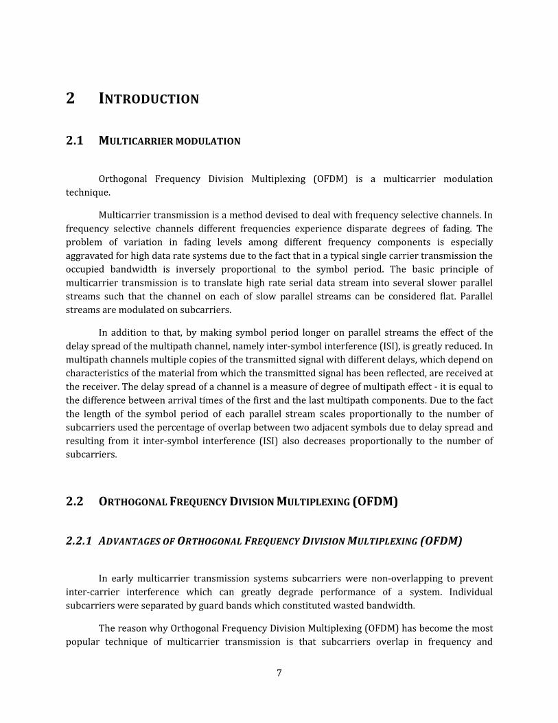
2 INTRODUCTION
2.1 MULTICARRIER MODULATION
Orthogonal Frequency Division Multiplexing (OFDM) is a multicarrier modulation
technique.
Multicarrier transmission is a method devised to deal with frequency selective channels. In
frequency selective channels different frequencies experience disparate degrees of fading. The
problem of variation in fading levels among different frequency components is especially
aggravated for high data rate systems due to the fact that in a typical single carrier transmission the
occupied bandwidth is inversely proportional to the symbol period. The basic principle of
multicarrier transmission is to translate high rate serial data stream into several slower parallel
streams such that the channel on each of slow parallel streams can be considered flat. Parallel
streams are modulated on subcarriers.
In addition to that, by making symbol period longer on parallel streams the effect of the
delay spread of the multipath channel, namely inter-symbol interference (ISI), is greatly reduced. In
multipath channels multiple copies of the transmitted signal with different delays, which depend on
characteristics of the material from which the transmitted signal has been reflected, are received at
the receiver. The delay spread of a channel is a measure of degree of multipath effect - it is equal to
the difference between arrival times of the first and the last multipath components. Due to the fact
the length of the symbol period of each parallel stream scales proportionally to the number of
subcarriers used the percentage of overlap between two adjacent symbols due to delay spread and
resulting from it inter-symbol interference (ISI) also decreases proportionally to the number of
subcarriers.
2.2 ORTHOGONAL FREQUENCY DIVISION MULTIPLEXING (OFDM)
2.2.1 ADVANTAGES OF ORTHOGONAL FREQUENCY DIVISION MULTIPLEXING (OFDM)
In early multicarrier transmission systems subcarriers were non-overlapping to prevent
inter-carrier interference which can greatly degrade performance of a system. Individual
subcarriers were separated by guard bands which constituted wasted bandwidth.
The reason why Orthogonal Frequency Division Multiplexing (OFDM) has become the most
popular technique of multicarrier transmission is that subcarriers overlap in frequency and

8
therefore bandwidth utilization increases by up to 50%. Overlapping subcarriers is allowed
because in OFDM modulation subcarriers are orthogonal to each other. Moreover, OFDM
modulation/demodulation takes form of inverse DFT/DFT which can be efficiently implemented in
hardware using Fast-Fourier Transform algorithm.
2.2.2 OFDM MODULATION
In OFDM transmitter N complex-value source symbols Xk k=0,1,...N-1, which can come from
any constellation, such as QPSK or QAM, are modulated onto N orthogonal subcarriers - inverse
Fourier-Transform complex exponentials evaluated at subcarrier frequencies fk :
𝑥 𝑡 = 𝑋𝑘 ∗ 𝑒𝑗2𝜋𝑓𝑘 𝑡𝑁−1𝑘=0 (1)
In a digital transmitter t=nTs where Ts is the sampling period. Subcarriers frequencies are
uniformly distributed:
fk=k*fs k=0,1, ... N-1 (2)
Frequency spacing fs is equal to 1
𝑁𝑇𝑠 in order to preserve orthogonality between subcarriers.
The final form of OFDM transmission takes a form of inverse-Fast-Fourier Transform:
𝑥𝑛 = 𝑥 𝑛𝑇𝑠 = 𝑋𝑘 ∗ 𝑒 𝑗2𝜋𝑛𝑘
𝑁𝑁−1𝑘=0 n=0,1,...N-1 (3)
N-sample long x sequence is called OFDM symbol and its duration is equal to N*Ts.
2.2.3 OFDM DEMODULATION
ADC at the receiver receives an analog signal which is a result of convolution of the
transmitted OFDM symbol x(t) with the channel impulse response plus noise:
r(t)= 𝑟(𝑡 − 𝜏)∞
−∞∗ 𝜏, 𝑡 + 𝑛(𝑡) (1)
OFDM demodulation takes a form of Fast-Fourier Transform of the sampled received signal r(t)
(after removal of Ng samples of the guard interval):
𝑅𝑘 = 𝑟𝑛 ∗ 𝑒−𝑗2𝜋𝑛𝑘
𝑁𝑁−1𝑘=0 k=0,1,...N-1 (2)
Since inter-carrier interference (ICI) is avoided by maintaining orthogonality between subcarriers
the channels (Hk’s) at subcarriers’ frequencies can be treated independently and the demodulated
OFDM symbol in a frequency domain can be written as:

9
Rk=Hk*Xk+Nk (3)
After channel estimation which yields complex-valued channel attenuation factors Hk at
each subcarrier’s frequency the decoded k-th transmitted data symbol 𝑋 𝑘can be obtained through
the following transformation:
𝑋 𝑘=QAM/QPSK de-mapper (𝑅𝑘
𝐻𝑘)
2.2.4 GUARD INTERVAL
In order to eliminate inter-symbol interference (ISI) due to the multipath channel a guard
interval is inserted at the beginning of each OFDM symbol in the OFDM transmitter. The length of
the guard interval - Ng is set such it is greater than the delay spread of the channel. The guard
interval is formed by copying last Ng samples of an OFDM symbol and appending them at the
beginning of the same OFDM symbol.
The guard interval is made by design longer than the delay spread of the channel therefore within
the symbol period only multiple copies of the same symbol are combined - no ISI occurs.
Due to the fact that I did not design my transceiver for a specific channel I used 802.11a
length of the guard interval – 16 samples.
2.3 SYSTEM ARCHITECTURE
The circuit diagram for the entire transceiver’s structure is in Appendix Section 8.1 Figure 12.
2.3.1 DESCRIPTION OF THE OFDM TRANSCEIVER’S COMPONENTS
2.3.1.1 COARSE SYNCHRONIZATION COMPONENTS
Coarse synchronization is used to roughly estimate the start of an OFDM symbol and the
fractional frequency offset (FCO) (for a detailed description of the coarse synchronization
mechanism see Section 4.4.2). The coarse synchronization mechanism is the first processing unit in
the receiver.
COARSE SYMBOL TIMING OFFSET SYNCHRONIZATION COMPONENTS The chain of the following components in the circuit diagram is responsible for calculation of
the timing offset metric which is used for the coarse symbol timing synchronization - determination

10
of the start of an OFDM symbol (please refer to eq. (4) in Section 4.2.1 for the timing offset metric
expression):
16-element shift register
bank of multipliers
multi-operand adders
Vectoring CORDIC unit
TO multiplier
The autocorrelation calculation embedded in the expression for the timing offset metric has a
special form in which multiplication of the consecutive samples in the two halves of the 15-sample
long autocorrelation window is replaced by the multiplication of the samples “going” back and
forward in time with respect to the center sample in the autocorrelation window.
15-element shift register creates a perfect structure for this special form of the autocorrelation
calculation (it consists of 15 elements because the preamble used for the coarse synchronization
consists of 16-sample long “mini” preambles, as described in Section 4.3, and the calculation
symmetry inherent in the timing offset metric expression requires an odd number of elements).
The eight pairs of complex multiplication terms in the timing offset metric expression are tapped off
from the shift register and fed into a bank of multipliers.
The bank of multipliers consists of four “mini” banks– each “mini” bank of 8 multipliers is
responsible for calculation of one of the four cross-products of the real and the imaginary parts of
the eight complex pairs. The resulting cross-product terms are summed up using multi-operand
adders (one adder for the real part of the multiplication result and the other one for the imaginary
part). The outputs of the adders are fed to the Vectoring CORDIC unit which calculates the modulus
of the complex-valued timing offset metric (the Vectoring CORDIC unit is used as a rectangular-to-
polar coordinate converter).
Next, the modulus of the timing offset metric is squared using TO multiplier to de-emphasize
erroneous peaks in the autocorrelation function embedded in the timing offset metric expression.
COARSE FRACTIONAL FREQUENCY OFFSET SYNCHRONIZATION COMPONENTS Coarse FCO Metric Calculation Unit – this unit calculates the coarse frequency offset metric (see
eq. (2) in Section 4.2.1) using a serial multiplier/accumulator mechanism (for a description of the
serial multiplier/accumulator mechanism see Section 4.4.2.2). The frequency offset metric is
converted to the actual frequency offset value using the Vectoring CORDIC unit.
FINE SYNCHRONIZATION COMPONENTS
Fine synchronization is used for fine-tuning the estimates of the synchronization errors (the
symbol timing offset and the fractional frequency offset) obtained in the course synchronization
stage. It is the second processing unit in the receiver.

11
COMPONENTS COMMON FOR BOTH THE FINE SYMBOL TIMING OFFSET AND THE FINE
FRACTIONAL FREQUENCY OFFSET SYNCHRONIZATION De-rotator (Para-CORDIC) – it de-rotates the received samples by the coarse frequency offset.
Both the fine symbol timing offset synchronization and the fine frequency offset synchronization
components use as a source of the received data samples the de-rotated samples produced by this
unit. The de-rotator unit is based on CORDIC algorithm in rotation mode (for a detailed description
of the algorithm and its hardware implementation, called Para-CORDIC, see Section 3.2.4).
FINE SYMBOL TIMING OFFSET SYNCHRONIZATION COMPONENTS Cross-correlator – this unit calculates the cross-correlation between the received de-rotated
samples of the second preamble (Preamble 2) and the reference Preamble 2 samples stored in a
look-up table (for a description of the Preamble 2 structure see Section 4.3). The cross-correlation
is calculated for an 11-delay window around the start of an OFDM symbol determined by the coarse
symbol timing offset synchronization. The maximum of the cross-correlation values (one value for
one delay in the cross-correlation window) determines the start of an OFDM symbol for decoding
purposes.
FINE FRACTIONAL FREQUENCY OFFSET SYNCHRONIZATION COMPONENTS Fine FCO Metric Calculation Unit – this unit calculates the coarse frequency offset metric for each
delay in the cross-correlation window. Similar to the coarse synchronization counterpart it uses a
serial multiplier/accumulator mechanism and its output is converted to the actual frequency offset
value using the Vectoring CORDIC unit.
CHANNEL ESTIMATION
Channel estimation is used to estimate complex-valued frequency attenuation factors at all
subcarriers’ frequencies from the FFT of the received pilot samples and the reference pilot samples
(for a detailed description of the channel estimation mechanism see Section 4.4.4). The obtained
attenuation factors are used to equalize the data symbols using an equalizer.
CHANNEL ESTIMATION COMPONENTS Channel Frequency Response Register – this unit consists of a shift register storing the complex-
valued frequency attenuation factors in polar coordinates for all subcarriers’ frequencies.
Pilot Look-up Table – a look-up table used to store the reference samples of the pilot symbol.
COMPONENTS COMMON FOR BOTH CHANNEL ESTIMATION AND EQUALIZATION/DATA
DECODING FFT64 – 64-point Fast-Fourier Transform unit used to demodulate OFDM symbols (see eq. (2) in
Section 2.2.3). An identical unit is used to do OFDM modulation of the source symbols in the
transmitter (see eq. (1) in Section 2.2.2)

12
Polar-to-Rectangular Coordinate Converter – channel estimation and equalization are based on
a division operation of complex numbers in polar coordinates. The results obtained in these
processing units have to be converted back to rectangular coordinates for 16-QAM de-mapper.
Division Unit – this unit calculates division of the modulus of the FFT of the received pilot sample
by the modulus of the reference pilot sample in the channel estimation processing unit and the
modules of the FFT of the received data sample by the modulus of the channel frequency response
in the equalization/data decoding processing unit. The division operation is implemented using
CORDIC algorithm in vectoring mode of linear type (for a detailed description of the algorithm and
its hardware implementation see Section 3.2.3)
EQUALIZATION/DATA DECODING
An equalizer is used for compensation of the received sample by the complex-valued
frequency attenuation factor at a given subcarrier’s frequency (for a detailed description of
equalization/data decoding mechanism see Section 4.4.5). The equalizer is implemented using the
division unit.
EQUALIZATION/DATA DECODING COMPONENTS 16-QAM De-mapper – this unit maps the received data samples to one of the sixteen 16-QAM
constellation points.
3 ALGORITHMS USED IN THE OFDM TRANSCEIVER’S DESIGN
3.1 FAST-FOURIER TRANSFORM
3.1.1 ALTERNATIVE SOLUTIONS AND DESIGN CHOICE
As a specification reference for my OFDM transceiver’s parameters I used 802.11a modem
standard. In 802.11a standard 64-point Fast Fourier Transform processor is used to implement
OFDM modulation and demodulation.
I did an extensive research on efficient hardware implementation of Fast Fourier Transform
algorithm from which I concluded that the most crucial design aspect of the hardware
implementation of Fast Fourier Transform is a process of performing multiplication by complex
exponential factors, so called twiddle factors.

13
Fast-Fourier Transform Design Choice
Alternative Solutions Justification of Selection Decision
One can group available solutions to the "twiddle factors" multiplication problem into :
a brute force method by a regular multiplication
CORDIC algorithm based multiplication
hardwired multiplication using Carry-Save Adder Trees and Canonical Signed-Digit representation of twiddle factors
In the preliminary hardware cost analysis I ruled out the first option due to the fact that it is the most hardware resources expensive - each of 49 nontrivial multiplications for 64-point FFT requires 4 real multipliers - not viable solution due to lack of resources on the target Altera FPGA. CORDIC algorithm is an attractive solution due to its inherent efficient mechanism for performing a multiplication by a complex exponential. In addition to that, CORDIC-based multiplication architecture has a very regular structure therefore it is easily scalable (there is no difference in multiplication process for different sets of twiddle factors). However, in order to minimize latency multiple CORDIC modules have to be instantiated. Hardwired multiplication using Carry-Save Adder Trees and Canonical Signed-Digit representation of the twiddle factors is very hardware efficient method to perform multiplication because it only uses adders and shifters which are fast hardware components. The reason why I chose the algorithm based on the hardwired multiplication over CORDIC algorithm is because for the desired FFT order of 64 there are only 8 sets of unique constants which, with conditional interchange and negation operations, can perform all 49 nontrivial complex multiplications. This solution offers the best speed performance and great hardware savings as compared to CORDIC algorithm based alternative. CORDIC--based architecture would require multiple CORDIC modules to achieve the same latency.
14
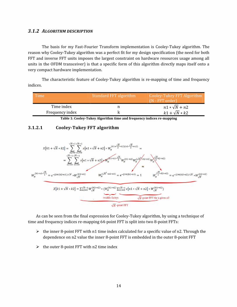
3.1.2 ALGORITHM DESCRIPTION
The basis for my Fast-Fourier Transform implementation is Cooley-Tukey algorithm. The
reason why Cooley-Tukey algorithm was a perfect fit for my design specification (the need for both
FFT and inverse FFT units imposes the largest constraint on hardware resources usage among all
units in the OFDM transceiver) is that a specific form of this algorithm directly maps itself onto a
very compact hardware implementation.
The characteristic feature of Cooley-Tukey algorithm is re-mapping of time and frequency
indices.
Time Standard FFT algorithm Cooley-Tukey FFT Algorithm (N - FFT order)
Time index n 𝑛1 ∗ 𝑁 + 𝑛2 Frequency index k 𝑘1 + 𝑁 ∗ 𝑘2
Table 1: Cooley-Tukey Algorithm time and frequency indices re-mapping
3.1.2.1 Cooley-Tukey FFT algorithm
As can be seen from the final expression for Cooley-Tukey algorithm, by using a technique of
time and frequency indices re-mapping 64-point FFT is split into two 8-point FFTs:
the inner 8-point FFT with n1 time index calculated for a specific value of n2. Through the
dependence on n2 value the inner 8-point FFT is embedded in the outer 8-point FFT
the outer 8-point FFT with n2 time index

15
3.1.3 HARDWARE IMPLEMENTATION
3.1.3.1 Overall architecture
In the design of the Fast-Fourier Transform unit I used ideas presented in [6].
The expression for Cooley-Tukey algorithm maps directly into the following hardware
implementation:
Figure 1: Fast-Fourier Transform unit circuit diagram.
FFT hardware units: I/P (input) unit - consist of a bank of 57 registers for both the real and the imaginary parts
of the serial input. At each clock cycle a serial data is shifted in at 56th position register
(counting from 0) and the data in the rest 56 registers is shifted down one register at a time.
The registers at 0, 8, 16, 24, 32, 40, 48 and 56th positions are tapped off to produce
𝑥[𝑛1 ∗ 8+n2] samples for the inner 8-point FFT unit (where n1=0,1,2.. 7).
Inner 8-point FFT unit - n1 is a time index calculated for a specific n2 value
Multiplier unit - multiplication of the inner 8-point FFT outputs by the twiddle factors
INTERM Unit – an intermediate storage unit. It consists of a bank of 64 registers for both
the real and the imaginary parts of data coming from the multiplier unit. Its function is to
collect all 64 inner 8-point FFT outputs multiplied by the twiddle factors for all eight n2
values. Similarly to I/P unit register bank 0, 8, 16, 24, 32, 40,48 and 56th positions are
tapped off to produce the input to the outer 8-point FFT
Outer 8-point FFT unit - n2 is a time index
O/P (output) unit - consists of a bank of 57 registers, similar to I/P unit. During the eight
clock cycles of the 8-point outer FFT unit operation 64-point FFT samples are shifted in
from the outer 8-point FFT at 0, 8, 16, 24, 32, 40,48 and 56th positions. At each clock cycle
data is shifted down one register at a time in the register bank and the serial out data is
shifted out from the 0th position register.
16
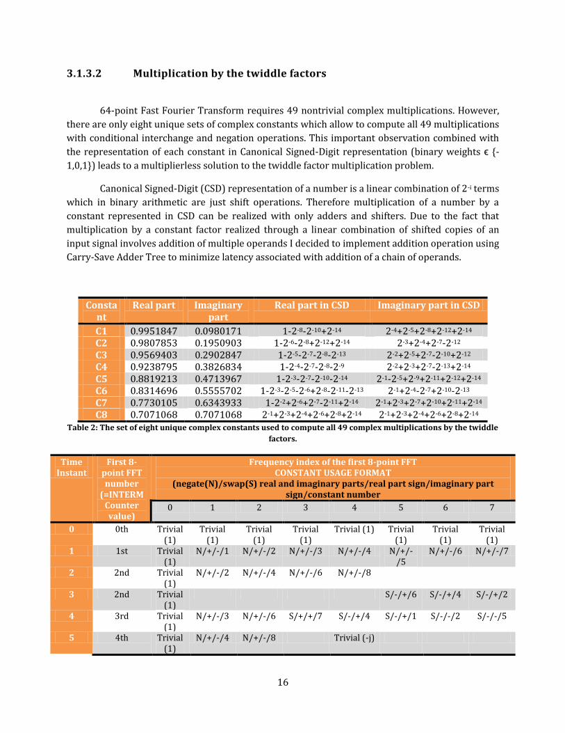
3.1.3.2 Multiplication by the twiddle factors
64-point Fast Fourier Transform requires 49 nontrivial complex multiplications. However,
there are only eight unique sets of complex constants which allow to compute all 49 multiplications
with conditional interchange and negation operations. This important observation combined with
the representation of each constant in Canonical Signed-Digit representation (binary weights ϵ {-
1,0,1}) leads to a multiplierless solution to the twiddle factor multiplication problem.
Canonical Signed-Digit (CSD) representation of a number is a linear combination of 2-i terms
which in binary arithmetic are just shift operations. Therefore multiplication of a number by a
constant represented in CSD can be realized with only adders and shifters. Due to the fact that
multiplication by a constant factor realized through a linear combination of shifted copies of an
input signal involves addition of multiple operands I decided to implement addition operation using
Carry-Save Adder Tree to minimize latency associated with addition of a chain of operands.
Constant
Real part Imaginary part
Real part in CSD Imaginary part in CSD
C1 0.9951847 0.0980171 1-2-8-2-10+2-14 2-4+2-5+2-8+2-12+2-14 C2 0.9807853 0.1950903 1-2-6-2-8+2-12+2-14 2-3+2-4+2-7-2-12 C3 0.9569403 0.2902847 1-2-5-2-7-2-8-2-13 2-2+2-5+2-7-2-10+2-12 C4 0.9238795 0.3826834 1-2-4-2-7-2-8-2-9 2-2+2-3+2-7-2-13+2-14 C5 0.8819213 0.4713967 1-2-3-2-7-2-10-2-14 2-1-2-5+2-9+2-11+2-12+2-14 C6 0.8314696 0.5555702 1-2-3-2-5-2-6+2-8-2-11-2-13 2-1+2-4-2-7+2-10-2-13 C7 0.7730105 0.6343933 1-2-2+2-6+2-7-2-11+2-14 2-1+2-3+2-7+2-10+2-11+2-14 C8 0.7071068 0.7071068 2-1+2-3+2-4+2-6+2-8+2-14 2-1+2-3+2-4+2-6+2-8+2-14
Table 2: The set of eight unique complex constants used to compute all 49 complex multiplications by the twiddle
factors.
Time Instant
First 8-point FFT number
(=INTERMCounter value)
Frequency index of the first 8-point FFT CONSTANT USAGE FORMAT
(negate(N)/swap(S) real and imaginary parts/real part sign/imaginary part sign/constant number
0 1 2 3 4 5 6 7
0 0th Trivial (1)
Trivial (1)
Trivial (1)
Trivial (1)
Trivial (1) Trivial (1)
Trivial (1)
Trivial (1)
1 1st Trivial (1)
N/+/-/1 N/+/-/2 N/+/-/3 N/+/-/4 N/+/-/5
N/+/-/6 N/+/-/7
2 2nd Trivial (1)
N/+/-/2 N/+/-/4 N/+/-/6 N/+/-/8
3 2nd Trivial (1)
S/-/+/6 S/-/+/4 S/-/+/2
4 3rd Trivial (1)
N/+/-/3 N/+/-/6 S/+/+/7 S/-/+/4 S/-/+/1 S/-/-/2 S/-/-/5
5 4th Trivial (1)
N/+/-/4 N/+/-/8 Trivial (-j)
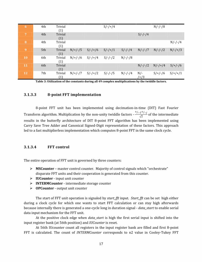
17
6 4th Trivial (1)
S/-/+/4 N/-/-/8
7 4th Trivial (1)
S/-/-/4
8 4th Trivial (1)
N/-/-/4
9 5th Trivial (1)
N/+/-/5 S/-/+/6 S/-/+/1 S/-/-/4 N/-/-/7 N/-/-/2 N/-/+/3
10 6th Trivial (1)
N/+/-/6 S/-/+/4 S/-/-/2 N/-/-/8
11 6th Trivial (1)
N/-/-/2 N/-/+/4 S/+/-/6
12 7th Trivial (1)
N/+/-/7 S/-/+/2 S/-/-/5 N/-/-/4 N/-/+/3
S/+/-/6 S/+/+/1
Table 3: Utilization of the constants during all 49 complex multiplications by the twiddle factors.
3.1.3.3 8-point FFT implementation
8-point FFT unit has been implemented using decimation-in-time (DIT) Fast Fourier
Transform algorithm. Multiplication by the non-unity twiddle factors - + − 1+ − 𝑗
2 of the intermediate
results in the butterfly architecture of DIT 8-point FFT algorithm has been implemented using
Carry Save Tree Adder and Canonical Signed-Digit representation of these factors. This approach
led to a fast multiplierless implementation which computes 8-point FFT in the same clock cycle.
3.1.3.4 FFT control
The entire operation of FFT unit is governed by three counters:
MSCounter – master control counter. Majority of control signals which "orchestrate"
disparate FFT units and their cooperation is generated from this counter.
IUCounter - input unit counter
INTERMCounter - intermediate storage counter
OPCounter - output unit counter
The start of FFT unit operation is signaled by start_fft input. Start_fft can be set high either
during a clock cycle for which one wants to start FFT calculation or can stay high afterwards
because internally there is generated a one-cycle long in duration signal - data_start to enable serial
data input mechanism for the FFT unit.
At the positive clock edge when data_start is high the first serial input is shifted into the
input register bank (at 56th position) and IUCounter is reset.
At 56th IUcounter count all registers in the input register bank are filled and first 8-point
FFT is calculated. The count of INTERMCounter corresponds to n2 value in Cooley-Tukey FFT

18
expression hence it specifies the number of currently being processed inner 8-point FFT and
coordinates a shifting in process in the intermediate storage register bank according to n2 value.
Because of that INTERMCounter has to be reset at 56th count of IUCounter. In order to centralize
control around MSCounter MSCounter is enabled by start_count control signal two cycles before the
first 8-point FFT is computed (when IUCounter=54). This way the reset of INTERMCounter can be
evoked through the main control counter.
As can be seen in Table 3. , the constants 2,4 and 6 are reused two times for the 2nd and the
6th inner FFT and the constant 4 is reused 4 times. Therefore shifting down in the input register
bank and an update of the intermediate storage bank are suspended for one cycle for the 2nd and
the 6th inner FFT and for three clock cycles for the 4th inner FFT by means of suspend_shift and
suspend_INTERMCounter control signals.
There are three temporary registers inside the input unit designed specifically to hold input
data during suspension of the shifting mechanism. Every clock cycle a serial input data is shifted
into temporary register 1. The existing data stored in the temporary registers is shifted down one
register at a time until all three temporary registers hold the last input data samples. At this point
shifting in and down operations in the temporary registers are suspended through
suspend_tempregUpdate signal.
Utilization of temporary registers during suspension
Inner FFT number 0 2 2 2 3 4 4 4 4 5 6 6 7 Serial input data sample number (range: 0-63 )
57 58 59 60 61 62 63 ... .... ... ... ... ...
Temporary register 1 56 57 58 59 60 61 62 63 63 63 63 63 63
Temporary Register 2
55 56 57 58 59 60 61 62 62 62 62 62 62
Temporary register 3 54 55 56 56 58 59 60 61 61 61 61 61 61
Input register 56 56 57 58 58 59 60 60 60 60 61 62 62 63
Suspend_shift
suspend_tempregUpdate
Table 4: The bordered fields indicate which temporary register is used as a source of the input data for the 56th
position in the input register bank after release of suspension. The red shading indicates active status of the
suspension control signals. As can be seen in the table no input data is lost during suspension of the shifting
mechanism.
Once the last (8th) inner FFT computation is finished on the next clock cycle all inner FFT
outputs, which have been multiplied by the twiddle factors, are available in the intermediate
storage register bank for the outer FFT unit. From this point on the outer 8-point FFT begins its
operations.
For the next 8 clock cycles during which all 8 outer FFTs are calculated shifting down in the
intermediate register bank is enabled (enable_INTERMshift) in order to provide correct input data
to the outer 8-point FFT unit.

19
Due to the fact that the 8-point FFT unit produces its result in the same clock cycle with a
stable logical value before the negative clock edge an update of the output register bank's 0, 8, 16,
24, 32, 40,48 and 56th positions is done on the negative edge in the same clock cycle. The update
takes place during 8 cycles of the outer FFT unit operation (it is enabled via enable_OPUpdate
control signal).
The reason why the output register bank is updated on the negative clock edge is that it
allows to produce a serial output right at the next positive edge without introducing additional
delay. This approach cuts the serial output latency in half because instead of using one clock cycle
for an update and one cycle for shifting out of the FFT data only one cycle is used for both
operations.
The serial output of FFT samples is controlled by OPcounter which value corresponds to the
FFT sample number currently being output.
OPcounter is reset in the same clock cycle as the first outer 8-point FFT and counts up to 63 (total of
64 FFT samples).
The serial output of the 64-point FFT samples continues as long as enable_serialout stays high.
Enable_serialout signal stays high for 64 cycles starting from the first outer FFT unless the FFT unit
is continuously active in which case it stays high until the last batch of 64 data FFT samples are
output.
3.1.3.5 INVERSE FAST FOURIER TRANSFORM
The only change in the Fast Fourier Transform unit required to implement Inverse Fast
Fourier Transform concerns swapping of the real and the imaginary parts of both the input serial
data and the output serial data. A signal inverse_fft triggers the swapping mechanism.
3.2 CORDIC ALGORITHM
3.2.1 INTRODUCTION
CORDIC (COrdinate Rotation DIgital Computer) algorithm is a multiplierless method to
perform a vector rotation. The fundamental principle of CORDIC algorithm is based on
decomposition of a rotation angle θ onto the discrete bases wn=arctan(2-n) :
𝜃 = σ𝑘∞𝑘=0 𝑤𝑛 (1)
where σ𝑘 − 𝑟𝑜𝑡𝑎𝑡𝑖𝑜𝑛 𝑑𝑖𝑟𝑒𝑐𝑡𝑖𝑜𝑛
Instead of performing a vector rotation in one step by a given rotation angle θ:

20
xnew= cos(θ)x0-sin(θ)y0 (2)
ynew= sin(θ)x0+ cos(θ)y0 (3)
CORDIC algorithm iteratively rotates a vector (x0,y0) by the rotation angle's discrete bases:
xn+1= cos(σnwn)xn-sin(σnwn)yn (4)
yn+1= sin(σnwn)xn+ cos(σnwn)yn (5)
Given an initial vector (x0,y0) and a rotation angle θ the general form of radix-2 CORDIC algorithm
is:
𝑥𝑛+1 = 𝑥𝑛 −𝑚σnyn2−σn (6)
𝑦𝑛+1 = 𝑦𝑛 + σn xn 2−σn (7)
𝑧𝑛+1 = 𝑧𝑛 − σnwn (8)
Type m wn Rotation mode 𝛔𝐧 = 𝐬𝐢𝐠𝐧(𝐳𝐧)
Vectoring mode 𝛔𝐧 = −𝐬𝐢𝐠𝐧(𝐲𝐧)
Circular 1 arctan(2-n) xn → K(x0cos(z0)-y0sin(z0)) yn → K(y0cos(z0)+x0sin(z0)) zn → 0
𝑥𝑛 → 𝐾 𝑥02 + 𝑦0
2 yn→0
zn→ z0+arctan(𝑦0
𝑥0)
Linear 0 2-n xn → 0 yn → y0+x0z0
zn → 0
xn → x0
yn → 0
zn → z0 + 𝑦0
𝑥0
Table 5: Various forms of CORDIC Algorithm.
3.2.2 CORDIC ALGORITHM IN VECTORING MODE (CIRCULAR TYPE)
In the design of the CORDIC algorithm in vectoring mode of circular type hardware
implementation I used ideas presented in [10] and [13].
3.2.2.1 Applications in the OFDM transceiver

21
Applications of Vectoring CORDIC of Circular Type In the OFDM Transceiver
Function Alternative solution Justification of selection decision
Rectangular-to-polar coordinate
conversion required for a division
operation in the equalizer
Complex division in rectangular coordinates - rectangular-to-polar coordinate conversion is not needed.
Complex division is much more computationally efficient in polar coordinates. Comparison of resources usage for a complex division in:
rectangular coordinates: 6 real multiplications
and 1 real division polar coordinates:
1 real division and 1 subtraction
Modulus calculation of the complex timing
offset metric
Use two multipliers to calculate square of the modulus of the timing offset metric. There is no need for square root operation due to the fact that only square of the modulus of the timing offset metric is required for synchronization purposes (squaring operation de-emphasizes small magnitudes of the autocorrelation function).
Due to the fact that modulus calculation is needed for a rectangular-to-polar coordinate conversion I decided to reuse the existing hardware instead of introducing two additional multipliers.
Angle calculation of the complex
frequency offset metric (conversion of the frequency offset
metric to the frequency offset
value)
None CORDIC algorithm in vectoring mode is the most commonly used method for an angle calculation due to its efficient hardware implementation.
3.2.2.2 Alternative solutions and design choice
Characteristic of radix-2 CORDIC algorithm is that the number of iterations required for
convergence is equal to the desired bit precision. The direct correlation between the number of
iterations and precision is the main disadvantage of radix-2 CORDIC algorithm.
In order to decrease latency of radix-2 CORDIC algorithm the general expression for the
radix-2 CORDIC algorithm is extended to radix-4:

22
xi+1=xi+m*σi*yi*4-i (1)
yi+1=yi- σi*xi*4-i (2)
zi+1=zi-αm,i(σi) (3)
where αm,i(σi)= tan-1(σi*4-i) in rotation mode
σi*4-i in vectoring mode
σi={-2,1,0,1,2}
Radix-4 CORDIC Algorithm
Advantages (+) Disadvantages (-)
the number of iterations is halved (equal to n/2 where n is bit precision)
more complicated logic to evaluate rotation directions σi
non-constant scaling factor due to redundancy in rotation directions’ representation
Table 6: Advantages and disadvantages of radix-4 CORDIC algorithm.
I chose radix-4 over radix-2 implementation of the vectoring CORDIC algorithm due to the
fact that in some of the above listed functions required for synchronization tasks in the receiver
only an angle calculation is required. Therefore latency associated with it can be significantly
reduced as the number of iterations is halved and the angle calculation does not require scaling by a
non-constant scaling factor.
However, scaling cannot be avoided in the case of a modulus calculation and there is no
particular advantage of employing radix-4 variation. Nevertheless, both angle and modulus
calculations are based on the same logic for rotation directions’ evaluation hence introducing a
separate radix-2 CORDIC algorithm unit solely for the purpose of a modulus calculation would only
entail an additional hardware and no benefit in speed performance. Both radix-2 and radix-4 take
the same number of iterations (equal to n – number of precision bits) to compute modulus because
in the case of radix-4 CORDIC algorithm there are n/2 iterations for the uncompensated (by a
scaling factor) modulus calculation and n/2 iterations for the non-constant scaling factor
compensation using a linear CORDIC in vectoring mode.

23
3.2.2.4 Algorithm description
Radix-4 Vectoring CORDIC Algorithm
Using variable substitution wi=yi4i radix-4 CORDIC algorithm can be described with the
following set of equations:
xi+1=xi+mσiwi4-2i (4)
wi+1=4(wi-σixi) (5)
zi+1=zi-αm,1(σi) (6)
where m= 0 - linear type
1 - circular type
αm=0,1 = σi4-i - linear type
arctan(σi4-i) - circular type
Proof that the number of iterations required for convergence is halved compared to
radix-2 CORDIC algorithm
Preliminary derivation:
If the rotation direction σi in each iteration is selected according to the following criterion:
xi*σi-(2/3)* xi <= wi <= xi*σi+(2/3)* xi (7)
then wi <= (8/3)*xi.
Proof by induction:
w0<(8/3)*x0 because according to the criterion (7) w0<= (5/3)*x0 which is less than (8/3)*x0.

24
Assuming that the induction hypothesis is true for i-1 iterations the proof will be completed if it can
be shown that the hypothesis is also true for i-th iteration.
For i-1-th iteration the criterion becomes:
|wi-1| <= xi-1*σi-1+(2/3)* xi-1 (8)
From the expression for w we obtain wi-1:
wi=4wi-1-4 xi-1*σi-1 => wi-1=wi/4+4 xi-1*σi-1 (9)
Plugging in the expression for wi-1 into (5) the result is:
|wi|<=(8/3)xi (10)
Based on the proof presented above after n iterations w is bounded by (8/3)*xn.
The angle of the final coordinates x and y after n iterations can be expressed:
θ= tan-1(𝑦𝑛
𝑥𝑛) =tan-1(
𝑤𝑛4−𝑛
𝑥𝑛) (11)
Plugging in the bounded value for w (10) into the above angle expression (11):
θ=tan-1(wn*4-n/xn) <= tan-1((8/3)xn2-2n/xn) = tan-1((8/3)xn2-2n/xn)= tan-1((4/3)2-2n+1) (12)
Let's assume that the number of iterations for convergence of radix-2 CORDIC is 2n. The angle value
obtained in radix-4 CORDIC algorithm is slightly greater than after n iterations and less than after
2n+1 iterations in a radix-2 CORDIC counterpart therefore it can be concluded that convergence
occurs after half the number of iterations of radix-2 CORDIC algorithm.
A new selection function for rotation directions
σi = 2 if wi > Pi(2) (13)
1 if Pi(1) < wi≤ Pi(2)
0 if Pi(-1) < wi ≤ Pi(-1)
-1 if Pi(-2) < wi≤ Pi(-1)
-2 if wi ≤ Pi(-2)

25
Derivation of the selection function for the rotation directions
It can be concluded from the criterion (7), which is the sufficient condition for radix-4
CORDIC algorithm convergence, that selection regions of different rotation directions in the set {-2,-
1,0,1,2} overlap.
Design problem 1: Nontrivial evaluation of the criterion (7) due to overlapping regions.
Solution: Reformulation of the criterion (7) into a form which allows efficient mapping to a
hardware implementation.
Each of the selection regions for rotation directions has two boundary points:
L(σi)= (σi-(2/3))*xi – the lower boundary of a region
U(σi)= (σi+(2/3))*xi – the upper boundary of a region
A discrimination point Pi between two rotation directions’ selection regions should be set to a
value which is equidistant from the opposite boundaries of the overlap region and in addition to
that, it should be in the middle of the overlap region. Therefore Pi's are set as follows:
P(1)=(1/2)*xi – the threshold point for σi=0 and σi=1selection regions
P(-1)= -(1/2)*xi – the threshold point for σi=0 and σi=-1 selection regions
P(2)=(3/2)*xi – the threshold point for σi=1 and σi=2 selection regions
P(-2)= -(3/2)*xi – the threshold point for σi=-1 and σi=-2 selection regions
Design Problem 2: The threshold points are dependent on the current iteration’s x value therefore
they need to be evaluated at each iteration.
Solution: Due to the fact that xi is increasing with the iteration number i both the upper and the
lower boundaries are spreading out as they are function of xi. Therefore it is possible to find lowest
iteration number for which the threshold value lies inside the overlap region of all successive
iterations and therefore is common for all of them. This happens when the lower boundary of the
highest iteration crosses some i-th iteration upper boundary:
Llast iteration(σi) < =P(σi) <= Uith iteration(σi) (14)
26
The lowest i for which the boundaries cross determines the iteration number which in turn
determines a threshold for all the remaining iterations.
Plugging in the expressions for L, U and x (4) into the above expression (14) and solving for
i one obtains i=1 for P(+/-1) and i=2 for P(+/-2).
3.2.2.5 Hardware implementation decisions
Coding approach
My modular hardware implementation is based on the notion of iteration in CORDIC
algorithm. I created a separate module for one iteration which is parameterized with the iteration
number in order to evoke correct shifters in calculation of x, y and z variables. The main module
only calculates necessary threshold values (Pi({-2,1,1,2}))and instantiates an iteration module for
each iteration. The iteration modules pass their outputs to a next iteration in a sequence. Coding
around the notion of iteration allows an easy extension of the design into higher bit precision. The
extension is achieved by mere invocation of additional iteration modules. Modification of the
number of pipelining stages is also greatly simplified in this approach because it only requires a
placement of pipeline registers for x, w and z variables and the threshold values at a desired break
point between iterations.
Pipelining decisions
Taking into account the architecture of the synchronization mechanism in which samples
are processed as they arrive at the receiver high throughput of the vectoring CORDIC unit is not
required. It is due to the fact that small amount of samples, which is determined by the latency of
the first processing unit in the receiver – the timing offset metric calculation, are available for
parallel processing (The timing offset calculation has latency of four cycles - 4 cycles for modulus
calculation of the timing metric using vectoring CORDIC algorithm combined with multiplication of
samples of the timing metric. This leaves only four samples for parallel processing). As a
consequence, I decided to use the smallest number of pipeline stages. The minimum number of
stages was determined by the latency of the sequential data-path of the entire CORDIC iteration
chain. Using Quartus software timing analysis tool for Cyclone II FPGA I obtained the propagation
delay for the entire chain including time for loading input and output registers. For 27-MHz clock
frequency the minimum number of pipeline stages was determined to be two.

27
Hardware optimization
Both x and W variables are scaled to be within [0,1] range in order not to lose precision in
the fractional part during intermediate steps.
W and the threshold values P used in the selection function (13) can be truncated to speed
up the comparison process and yet lead to correct selection. The threshold value P is in the middle
of two boundaries L and U. Selection will be correct as long as precision of W will be sufficient to
allow W to be within a distance between P and either of the boundaries U and L. As a consequence,
the distance between P and either of the boundaries U and L has to be larger than precision of the
truncated W.
The distance between P and either of the boundaries is equal to (1/6)*xi.
Therefore
(1/6)*xi >=2-Wfractional (15)
where Wfractional is the number of fractional bits of W.
Plugging in an expression for xi (4) one can determine the number of fractional bits Wfractional to be at
least 5.
Instead of implementing a complicated comparator for both positive and negative numbers
for the rotation directions' selection function I decided to decode sign information of W and the
comparison points P(+/-1), P(+/-2). Using the sign information in "case" statement the rotation
directions' selection conditions of (13) for each set of W and P's signs could be simplified or even
neglected if for a given set of W and Ps signs they are unconditionally always true or false.
3.2.2.5 Scaling factor
The major drawback of the radix-4 modification of the CORDIC algorithm is nontrivial in
evaluation scaling factor which is not constant as in the case of radix-2 baseline version of the
algorithm. The scaling factor is a function of rotation directions due to redundancy in the rotation
directions' representation therefore it has to be evaluated for each set of input values:
K= 𝑘𝑖 =𝑛
2−1
𝑖=0 (1 + σi
2 ∗ 4−2𝑖)−1
2
𝑛
2−1
𝑖=0 (16)
where n=𝐵 𝑏𝑖𝑡𝑠 𝑝𝑟𝑒𝑐𝑖𝑠𝑖𝑜𝑛
2 - number of iterations.
B – bit precision (in my design I set B to 16)

28
Simplifications:
the scaling factor has be evaluated only for the first n/4+1 iterations (in the rest of
iterations it can be approximated by 1)
ROM size used for storing each iteration's sub-scaling factors ki (3𝑛
4+1 − the base of 3 comes
from the fact that each σi can take 3 values) can be greatly reduced to 3𝑛
8+1by using the first
two terms of Taylor expansion for the iteration number i >=floor(𝑛
8+ 1)
𝑘𝑖=1-1
2σi
2 ∗ 4−2𝑖 (17)
which can implemented using only add and shift operations.
The above simplifications reduce the number of multipliers to 2 for the first 4 iterations
(reusing one multiplier in the 2-stage pipeline implementation used in the transceiver) and ROM
size to 3𝑛
8+1for evaluation of the nontrivial scaling factor.
Compensation of the modulus by the scaling factor is done using radix-4 vectoring CORDIC
algorithm of linear type.
3.2.3 CORDIC ALGORITHM IN VECTORING MODE (LINEAR TYPE)
In the design of the CORDIC algorithm in vectoring mode of linear type hardware
implementation I used ideas presented in [10] and [13].
3.2.3.1 Applications in the OFDM transceiver
Applications Of Vectoring CORDIC of Linear Type In The OFDM Transceiver
Function Alternative solution Justification of selection decision
Division of the modulus of the FFT of the received sample by: the modulus of the
reference pilot in the channel estimator
the modulus of the channel frequency response at a given subcarrier’s frequency in the
Use any of the available division algorithms
There is no particular advantage in terms of speed in performing division by the means of vectoring CORDIC of linear type as opposed to standard division algorithms. The reason I chose to implement division using CORDIC algorithm is that the vectoring CORDIC algorithm of linear type is just a simplified

29
decoder
version of the vectoring CORDIC algorithm of circular type therefore I was able to reuse the hardware already designed for the circular type.
Compensation of modulus in vectoring CORDIC of circular type
3.2.3.2 Algorithm description
As can be seen from the expressions for x, w and z variables in the radix-4 modification to
the vectoring CORDIC algorithm (equations 4-6 in section 3.2.2.4) a linear type variation can be
treated as a simplified version of a circular type counterpart. In linear coordinates m=0 therefore x
is constant for the entire CORDIC algorithm operation. Moreover, instead of adding an arctangent
term to z variable we only add its argument which does not require a ROM lookup table for arctan
values as in the case of circular coordinates. However, the core of radix-4 CORDIC algorithm -
rotation directions' selection function is exactly the same and hence the description of operation of
a circular counterpart and hardware optimization techniques used for the selection function from
the previous section applies to the linear type.
The major complication in comparison to circular coordinates concerns normalization
(scaling) of the input values. During a preliminary testing of the MATLAB floating point
implementation I noticed that algorithm only converges if both initial x and y coordinates are of the
same order of magnitude.
Normalization (Scaling) Procedure
Normalization step Function Normalize (scale) to 1 (shift until MSB is at binary 1 weight position) in the maximum allowable fractional part 16-bit fixed-point representation.
Minimize error propagation in between iterations due to insufficient precision of the intermediate results.
Scale a smaller coordinate of x and y to be of the same order as the other coordinate (shift until MSB position matches bit position of the other coordinate).
Convergence requirement
The maximum allowable fractional part in the 16-bit normalized fixed-point representation
of x and y is 13 bits. The absolute value of initial x and y coordinates is taken prior to normalization
in order to eliminate -1 and -2 rotation directions in the first iteration (the sign of the division
result - the final value of z variable is adjusted at the end based on the signs of initial x and y
coordinates).

30
Out of three variables x, y and z the minimum range of the integer part required for the
convergence of the CORDIC algorithm is determined solely by W variable because:
x variable stays constant (equal to the initial normalized to 1 x value) during the entire
CORDIC algorithm operation
z variable which converges to a division result of x and y coordinates which for the
normalized to 1 x and y values should not exceed 2
W is decreasing and converges to 0 therefore its value only on the first iteration determines
the required integer part range. Due to the fact that -2 and -1 rotation directions have been
eliminated by taking the absolute value prior to normalization the worst case (the highest
integer part of W on the first iteration) happens for 0 rotation direction on the first
iteration. The worst case value is bounded by 4 therefore we need at least 3 bits plus 1 bit
for a sign in the normalized x and y representation to ensure convergence and minimize
precision loss in the intermediate steps.
3.2.4 CORDIC ALGORITHM IN ROTATION MODE (PARA-CORDIC)
In the design of the CORDIC algorithm in rotation mode hardware implementation I used
ideas presented in [3],[5] and [12].
3.2.4.1 Applications in the OFDM transceiver
Applications of CORDIC Algorithm In Rotation Mode In the OFDM transceiver Application Alternative Solution Justification of Selection Decision
Direct Digital Synthesis (DDS)
Using multipliers and sine and cosine ROMs to compute a vector rotation.
Large frequency resolution in the case of DDS and, in more general case, resolution of the sine and cosine functions’ arguments requires large ROM sizes for sine and cosine values storage. Aside from the increased hardware resources usage larger ROMs induce higher power consumption and slower access times. ROM size issue is aggravated by the fact that in quadrature modulation both sine and cosine ROMs are needed. The need for both sine and cosine translations was the
De-rotation of a received sample by the frequency offset

31
main motivation behind employment of CORDIC algorithm as an up/down-converter. Moreover, multipliers used in a standard ROM-based DDS implementation cannot be reused due to its constant engagement in modulation and demodulation process during transceiver's operation.
3.2.4.2 Alternative solutions and design choice
CORDIC algorithm in rotation mode calculates coordinates of a vector (x0,y0) rotated by an angle z0.
CORDIC Algorithm In Rotation Mode Design Choice
Alternative Solutions Justification of Selection Decision
I did an extensive research on variations of a standard CORDIC algorithm in rotation mode. The available choices can be grouped into three categories:
standard radix-2 CORDIC algorithm with the number of micro-rotations (iterations) on the order of desired bit precision
higher radix modifications (such as, radix-4)
branching mechanism with parallel execution of two rotation directions at some iterations
The major problem with a standard form of the CORDIC algorithm regardless of radix choice is latency caused by a sequential character of rotation directions evaluation from the residual angle z (a rotation direction can be evaluated only when the previous iteration has finished). There have been introduced variations of CORDIC algorithm with a parallel execution of both rotation directions' data-paths and a branching mechanism used to select the correct result from one of the parallel execution branches along the execution chain. However, this option almost doubles hardware cost and does not completely eliminate the latency issue. The idea behind higher radix modifications (radix-4) is to ideally cut the number of iterations in half. However, higher radix variations introduce redundancy in the rotation directions’ representation which in turn causes non-constant scaling factor. Evaluation and compensation of the non-constant scaling factor aside from the fact that it entail an additional hardware consisting of ROM-based lookup tables for iterations’ sub-scaling factors and multipliers usually have an execution time on the order of radix-2 CORIDC algorithm. As a consequence, the overall execution time is still on the order of desired bit precision. I decided to implement a particular variation of CORDIC algorithm which offers the best compromise between all the aforementioned alternative options. It is called Para-CORDIC [5]. The name of the variation stems from the
32
fundamental principle on which this modification is based - parallel extraction of the rotation directions. Parallel extraction of the rotation directions eliminates the latency issue. It is achieved by recoding the rotation angle. However, hardware cost incurred due to recoding process is insignificant compared to the alternative solution to the latency issue - branching mechanism (the recoding hardware consists exclusively of 2-bit adders). In addition to that, Para-CORDIC is a radix-2 based modification therefore there is no extra hardware for scaling factor calculation because the scaling factor is constant and is pre-computed beforehand.
3.2.4.3 Algorithm description
A standard radix-2 CORDIC algorithm suffers from a critical path associated with evaluation
of the rotation directions from the residual angle z. It introduces additional latency which is
especially noticeable for higher bit precision.
The fundamental principle of Para-CORDIC variation [5] is decomposition of the rotation
angle into low and high parts for which a separate parallel extraction of rotation directions is
possible by the means of angle recoding.
Angle Recoding
Assumptions and notion convention:
the rotation angle is in range [0, π/4) - in section 3.2.4.5 extension to the full range [0,2π] is
introduced
B - denotes angle fractional bit precision (in my design I set B to 15)
Every angle in 2's complement representation - binary weights' coefficients ϵ {0,1} can be
converted to bipolar representation - binary weights' coefficients ϵ {-1,1} using the following
transformation:
𝜃 = −𝑏0 + 𝑏𝑘2−𝑘𝐵𝑘=1 = −𝑏0 + (2−𝑘−1 + (2𝑏𝑘 − 1)2−𝑘−1) = σ𝑖2
−𝑖 − 2−𝐵−1𝐵+1𝑖=1
𝐵𝑘=1 (1)
33
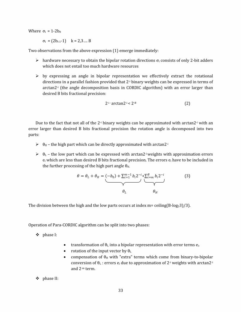
Where σi = 1-2b0
σi = (2bi-1-1) k = 2,3…. B
Two observations from the above expression (1) emerge immediately:
hardware necessary to obtain the bipolar rotation directions σi consists of only 2-bit adders
which does not entail too much hardware resources
by expressing an angle in bipolar representation we effectively extract the rotational
directions in a parallel fashion provided that 2-i binary weights can be expressed in terms of
arctan2-i (the angle decomposition basis in CORDIC algorithm) with an error larger than
desired B bits fractional precision:
2-i - arctan2-i < 2-B (2)
Due to the fact that not all of the 2-i binary weights can be approximated with arctan2-i with an
error larger than desired B bits fractional precision the rotation angle is decomposed into two
parts:
θH – the high part which can be directly approximated with arctan2-i
θL – the low part which can be expressed with arctan2-i weights with approximation errors
ei which are less than desired B bits fractional precision. The errors ei have to be included in
the further processing of the high part angle θH.
𝜃 = 𝜃𝐿 + 𝜃𝐻 = −𝑏0 + 𝑏𝑖2−𝑖𝑚−1
𝑖=1 + 𝑏𝑖2−𝑖𝐵
𝑖=𝑚 (3)
The division between the high and the low parts occurs at index m= ceiling(B-log23)/3).
Operation of Para-CORDIC algorithm can be split into two phases:
phase I:
transformation of θL into a bipolar representation with error terms ei.
rotation of the input vector by θL
compensation of θH with "extra" terms which come from binary-to-bipolar
conversion of θL : errors ei due to approximation of 2-i weights with arctan2-i
and 2-m term.
phase II:
𝜃𝐿 𝜃𝐻

34
conversion to a bipolar representation of the corrected θH (𝜃𝐻 ) with the
approximation errors of θL
rotation of x, y coordinates produced in phase I by the corrected θH
Phase I
First, θL is transformed from 2's complement into bipolar representation in which 2-i binary
weights are expressed as a linear combination of n(i) arctan terms (arctan2-i) and approximation
errors ei:
𝜃𝐿 = σi2−i − 2−m = σi
mi=1 arctan 2−si
j
+ ei − 2−mn(i)j=1
𝑚𝑖=1 (4)
Observation:
the ability to extract the rotation directions σi in parallel for θL comes at expense of
additional n(i) micro-rotations at i-th stage due to approximation of 2-i by arctan terms
A choice of a linear combination of arctan terms to approximate 2-i is not arbitrary.
The high part of the rotation angle θH is corrected by the extra terms which do not appear in a
standard CORDIC algorithm prior to rotation in phase II. The extra terms include: an extra term introduced in 2's complement-to-bipolar conversion - 2-m approximation errors ei of 2-i weights with arctan(2-i)
𝜃 =𝜃 + σi𝑚−1𝑖=1 ∗ 𝑒𝑖 − 2−𝑚 (5)
In order to maintain CORDIC convergence the following condition has to be met:
|𝜃 | < 2−𝑚+1 (6)
The authors in [5] devised an algorithm, called MAR, to find a linear combination which
satisfies the above condition (6). The algorithm finds the number of linear combination terms n(i)
and shift amounts for each term in the linear combination 𝑠𝑖𝑗
where
j=1,2,..n(i)
i – exponent of 2-i term for which an approximation is calculated.

35
For 15-bit fractional precision the number of linear combination terms n(i) and shift amounts for
each term are:
Binary weight Number of linear combination terms n(i)
Shift amounts for each term in the linear combination
2-1 2 1,5 2-i i=2,3,4 1 i
Table 7: The results of MAR algorithm for the 15-bit fractional bit precision of a rotation angle.
Example
2-1 = arctan(2-1) +arctan(2-5)
3.2.4.4 Hardware optimization
If the expressions for the final value of x and y are expanded by iteratively plugging in (in
decreasing iteration number) the i-th iteration expressions for x and y (equations 6-7 in Section
3.2.1) for all iterations one will notice that starting from the iteration number k>B/2 (in the case of
B=15 fractional bit precision k=8) all cross-products terms of the resulting expansion fall off the
precision range and therefore can be neglected. Therefore the expression for the final values of x
and y can be folded into a sum of terms involving exclusively k-th iteration values of x and y :
𝑥𝑘+1 = 𝑥𝑘 − 𝑦𝑘 σi
𝑘+𝐵2−1
𝑖=𝑘
2−𝑖
𝑦𝑘+1 = 𝑦 − 𝑥𝑘 σi
𝑘+𝐵2−1
𝑖=𝑘
2−𝑖
The sum in the above expression can be efficiently implemented using Carry-Save Adder
Tree which decreases significantly latency of the CORDIC data-path in comparison to traditional
CORDIC rotations in i>k iterations.
3.2.4.5 Range extension
CORDIC algorithm converges for a rotation angle in the range [0,𝜋
4 ). In the OFDM
transceiver various applications of CORDIC algorithm, such as up/down-conversion and de-rotation
of the received sample by the frequency offset, require full 2𝜋 range.

36
By exploiting symmetry of sine and cosine functions any angle in the range of [0,2π] can be
obtained from sine and cosine values of a related angle in the range [0, π/4) by decoding octant
information of the angle and conditional use of interchange and negate operations (3 MSB bits of
the normalized to 2𝜋 angle decode the octant number).
Due to the fact that CORDIC algorithm uses only angle information in [0,𝜋
4 ) range the input
rotation angle is expressed as a 19-bit number in order not to sacrifice fractional bit precision (1
bit to represent negative angles, 3 bits to represent maximum range - 2𝜋 value and the desired 15
bits for the fractional part).
Steps required for 2𝝅 range extension:
1. Normalize the rotation angle by dividing it by 2𝜋 such that the first MSB of the fractional
part has 𝜋 weight, the second MSB of the fractional part has 𝜋
2 weight and so on.
2. Decode the octant information of the angle - 3 MSB bits of the fractional part in the
normalized angle.
3. Strip-off 2 LSB bits of the 3 bits used for the octant decoding. If the octant number is odd
subtract from 𝜋
2 the stripped normalized angle (subtraction from
𝜋
2 in the normalized to 2𝜋
representation is equivalent to 2's complement operation). Now the normalized angle is in
the desired range [0, 𝜋
4) for CORDIC algorithm processing.
4. De-normalize the angle obtained in step 3 by multiplying it by 2𝜋 in order to restore
"binary" weights in the angle representation for CORDIC algorithm processing.
5. Conditional interchange of x and y coordinates of the input vector based on the octant
information (see a table below).
6. Conditional interchange and negation of final x and y coordinates based on the octant
information (see a table below).
Octant number (3 MSB of the fractional part of the normalized rotation angle)
Negate output x coordiante
Negate output y coordinate
Interchange output x and y coordinates
Interchange input x and y coordinates
0 NO NO NO NO 1 YES NO YES NO 2 NO YES NO YES 3 YES YES YES YES 4 YES YES NO NO 5 NO YES YES NO 6 YES NO NO YES

37
7 NO NO YES YES Table 8: Conditional interchange and negation operations for both the input and the output coordinates used in
the extension of the rotation angle’s range to 2π.
Example:
cos(240) =-1/2 = -sin(30) = -sin(240-180+(90-60))
4 SYNCHRONIZATION MECHANISM – OFDM RECEIVER DESIGN
4.1 SYNCHRONIZATION ERRORS
4.1.1 CARRIER FREQUENCY OFFSET
If there is a mismatch between frequencies of the transmitter and receiver’s free running
oscillators the resulting carrier frequency offset ∆f will result in rotation of the received symbol
samples by a constant frequency:
𝑟𝑖,𝑛 = 𝑒𝑗2𝜋∆ft |𝑡=𝑖 𝑁+𝑁𝑔 𝑇𝑠+𝑁𝑔𝑇𝑠+𝑛𝑇𝑠 (1)
where
N – the number of OFDM subcarriers
Ng – the length (in samples) of the guard interval
Ts - sampling period
i - symbol index
Strip-off 2 LSB of the 3 bits used for
octant decoding - 180 and 90 degrees
weights in the normalized angle
odd octant = > 2's complement =
subtraction from 90 degrees

38
n - time domain index
The frequency offset is usually normalized with respect to subcarrier spacing (𝑓𝑠=1
𝑁𝑇𝑠):
∆f=(IFO+FCO)*fs (2)
where
IFO – an integer part of the frequency offset ∆f with respect to subcarrier spacing
FCO – a fractional part of the frequency offset ∆f with respect to subcarrier spacing
Negative effects degrading receiver's performance:
attenuation in received magnitude
phase shift
ICI - inter-carrier interference
4.1.2 SYMBOL TIMING OFFSET
Symbol timing offset is an offset in the start of an OFDM symbol which corresponds to the
start of the FFT window.
The severity of negative effects depends on which of the following two possible scenarios occurs:
1. If the delay spread of the channel is shorter than the guard interval and the FFT window is
applied too early with an offset TO which is smaller than the difference between the delay
spread and the guard interval only an additional phase shift is introduced:
Rk=Xk*Hk𝑒−𝑗
2𝜋∗𝑇𝑂 ∗𝑘
𝑁𝑇𝑠 (1)
where
Xk – the frequency domain transmitted sample at k-th subcarrier
phase shift
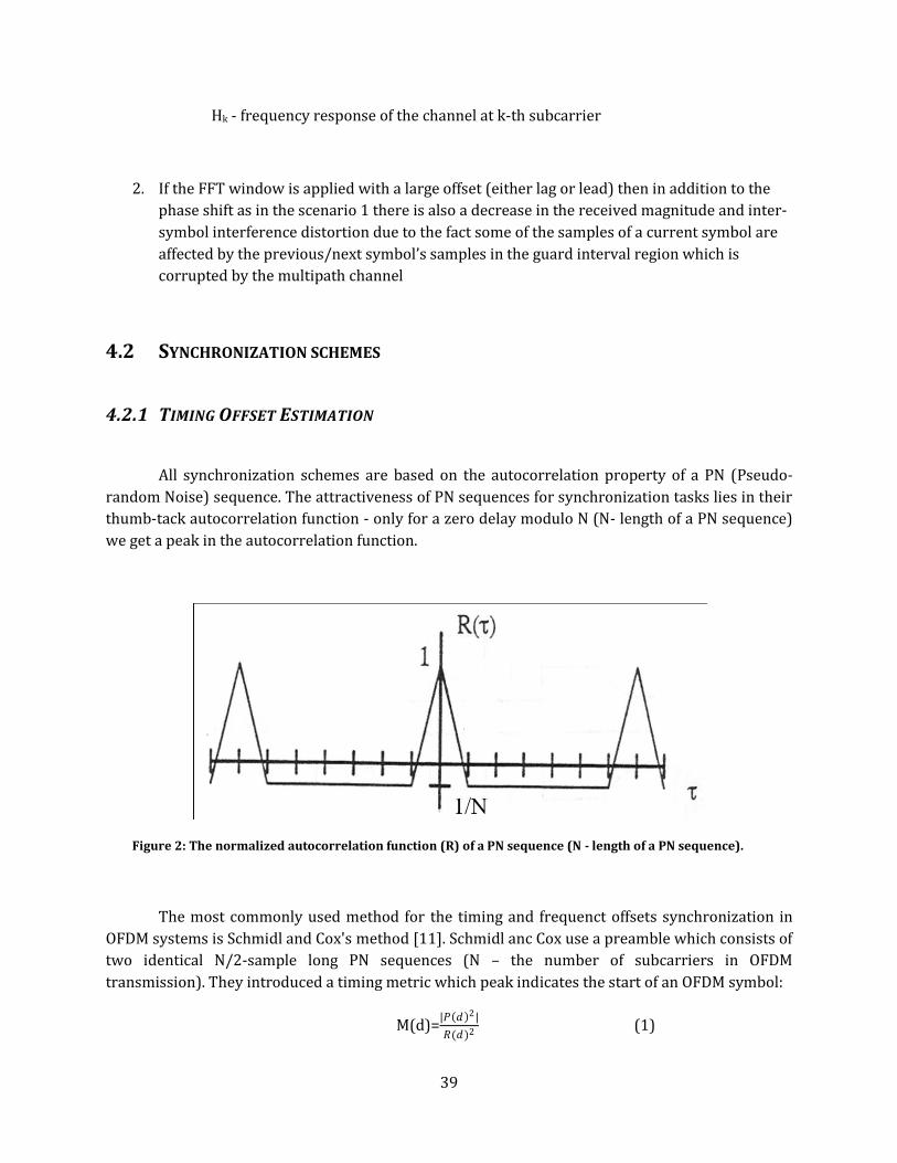
39
Hk - frequency response of the channel at k-th subcarrier
2. If the FFT window is applied with a large offset (either lag or lead) then in addition to the
phase shift as in the scenario 1 there is also a decrease in the received magnitude and inter-
symbol interference distortion due to the fact some of the samples of a current symbol are
affected by the previous/next symbol’s samples in the guard interval region which is
corrupted by the multipath channel
4.2 SYNCHRONIZATION SCHEMES
4.2.1 TIMING OFFSET ESTIMATION
All synchronization schemes are based on the autocorrelation property of a PN (Pseudo-
random Noise) sequence. The attractiveness of PN sequences for synchronization tasks lies in their
thumb-tack autocorrelation function - only for a zero delay modulo N (N- length of a PN sequence)
we get a peak in the autocorrelation function.
Figure 2: The normalized autocorrelation function (R) of a PN sequence (N - length of a PN sequence).
The most commonly used method for the timing and frequenct offsets synchronization in
OFDM systems is Schmidl and Cox's method [11]. Schmidl anc Cox use a preamble which consists of
two identical N/2-sample long PN sequences (N – the number of subcarriers in OFDM
transmission). They introduced a timing metric which peak indicates the start of an OFDM symbol:
M(d)=|𝑃 𝑑 2|
𝑅(𝑑)2 (1)

40
𝑃 𝑑 = 𝑟∗ 𝑑 + 𝑚 ∗ 𝑟(𝑑 + 𝑚 +𝑁
2
𝑁
2−1
𝑚=0 ) (2)
R(d)= |𝑟(𝑑 + 𝑚 +𝑁
2
𝑁
2−1
𝑚=0 )|2 (3)
The intuitive explanation why the above time metric (1) gives a peak at the start of an
OFDM symbol follows from the construction of the synchronization preamble. Since both halves of
the preamble are composed of the same PN sequence sum of products of a conjugate of a sample
from first half and a corresponding sample in the second half will be the largest due to the fact they
have the same phase and add up constructively.
Schmidl and Cox's method is very popular among OFDM designers, however, it suffers from
a plateau region around the peak. Using the timing offset metric, introduced by Schmidl and Cox,
one does not obtain a single peak at the start of an OFDM symbol but a plateau region which spans
the number of samples equal to the length of the guard interval minus the length of the channel
response.
The plateau region causes uncertainty in the start of an OFDM symbol therefore I started
researching variations on Schmidl and Cox’s method in order to find a solution which gives a
distinct single peak in the timing offset metric.
I found a desired variations in a paper by H. Minn [8] and a paper by P. Byungjoon [1]. Minn
uses a special structure of the synchronization preamble. Instead of using a preamble with two
identical PN sequennces in each halves Minn uses the following structure which emphasizes
differences between the peak timing metric and offset values and therefore achieves a
distinguishing single peak in the timing metric at the start of OFDM symbol:
[A A*A A*]
where A is N/4-sample long PN sequence and * denotes complex conjugate operator.
The modified timing offset metric takes the following form:
M(d)=|𝑃 𝑑 2|
𝑅(𝑑)2 (4)
𝑃 𝑑 = 𝑟∗ 𝑑 − 𝑚 ∗ 𝑟(𝑑 + 𝑚𝑁
2−1
𝑚=0 ) (5)
R(d)= |𝑟(𝑑 + 𝑚𝑁
2−1
𝑚=0 )|2 (6)

41
4.2.2 FRACTIONAL FREQUENCY OFFSET ESTIMATION
The only difference in phases between the first and the second half comes from the
frequency offset as the channel effect should cancel. The phase difference is equal to:
θ=2π*∆f *𝑇
2= π*∆f*T (1)
where
∆f – the fractional frequency offset (fractional with respect to subcarrier subspacing - 1
N∗Ts)
T – OFDM symbol duration
Therefore in order to find the fractional frequency offset we calculate an angle of the timing
metric at the start of the preamble symbol :
θ = angle(PFCO(d)) (2)
where PFCO(d) is expressed by (2) in section 4.2.1.
The obtained angle is converted into the frequency offset value using the phase difference equation
(1):
∆f=θ
𝜋𝑇 (3)
4.2.3 CHANNEL ESTIMATION
There are two groups of estimators used in OFDM systems:
Least-squares (LS) estimator
Mean-squared error (MMSE) estimator
Both estimators achieve the same performance in high signal-to-noise ratio environments. If
one knows a priori statistics of the channel, such as covariance matrix and SNR, MMSE estimator
can outperform LS estimator.
Due to the fact I did not design my transceiver for a specific channel type I decided to
implement LS estimator which takes the following form:
𝐻𝑘 =𝑟𝑒𝑐𝑒𝑖𝑣𝑒𝑑 𝑝𝑖𝑙𝑜𝑡 𝑓𝑟𝑒𝑞𝑢𝑒𝑛𝑐𝑦 𝑠𝑎𝑚𝑝𝑙𝑒 𝑎𝑡 𝑘 − 𝑡 𝑠𝑢𝑏𝑐𝑎𝑟𝑟𝑖𝑒𝑟 𝑓𝑟𝑒𝑞𝑢𝑒𝑛𝑐𝑦
𝑟𝑒𝑓𝑒𝑟𝑒𝑛𝑐𝑒 𝑝𝑖𝑙𝑜𝑡 𝑓𝑟𝑒𝑞𝑢𝑒𝑛𝑐𝑦 𝑠𝑎𝑚𝑝𝑒 𝑎𝑡 𝑘 − 𝑡 𝑠𝑢𝑏𝑐𝑎𝑟𝑟𝑖𝑒𝑟 𝑓𝑟𝑒𝑞𝑢𝑒𝑛𝑐𝑦
where
Hk – channel frequency response at k-th subcarrier

42
A pilot is an OFDM symbol which is known at the receiver and is used as a reference to
estimate corruption of the signal by the channel at a given subcarrier’s frequency. Pilots are
interleaved with data symbols.
4.3 ALTERNATIVE SOLUTIONS AND DESIGN CHOICE
In practice, synchronization is split into two phases:
coarse synchronization
fine synchronization
in order to improve accurancy of synchronization errors estimates and thereby improve
performance of a system. Synchronization done in a single step leaves significant residual errors. By
doing an initial coarse synchronization which brings initial large offsets in timing and frequency
into vicinity of the right answer and leaving fine-tunning for fine sychronization the residual errors
are small enough to not degrade performance of a system as opposed to a single-step
synchronization (the received signal is derotated by the estimate of the frequency offset
determined during the coarse synchronization stage and the processing of the fine synchronization
stage takes place on a corrected signal).
In my design I chose the following structure for the preambles responsible for coarse and
fine synchronization:
Preamble 1 GI Preamble 2 GI Pilot 1 GI Data 1 GI Data 2 ...
PN1 PN1 PN1 PN1 PN2
Coarse synchronization Fine Synchronization Channel Estimation
GI – guard interval
PN1 - 16-sample long preamble with Minn's PN sequence structure [A A*] where A is a
PN sequence of length 8
PN2- 64-sample long preamble with Minn's PN sequence structure [A A*] where A is a
PN sequence of length 32

43
Synchronization Implementation Design Choice
Synchronization Step
Alternative Solutions Justification of Selection Decision
Coarse synchronization
using standard Schmidl and Cox's method with a preamble consisting of two idential copies of a PN sequence of length 32
using the original Minn's method with two identical halves having complex conjugate symmetry which are built using 16-sample long PN sequence
I chose Minn's method over Schmidl and Cox's alternative because , as mentioned in the introduction, the standard Schmidl and Cox's timing metric suffers from a plateau region which introduces uncertainty in determination of the start of an OFDM symbol whereas Minn's method produces a single distinct peak at the start of a symbol. I decided to modify Minn's sychronization method taking into consideration hardware resources availability on the target FPGA – Cyclone II. Using Minn's single 64-sample long preamble would require 32 complex multiplications per one clock cycle to calculate the timing metric (each complex multiplication requires 4 real multiplications - total of 128 multiplications). Obviously, the number of embedded multipliers in Cyclone II FPGA is not sufficient. Even though one could implement it by extending the number of multipliers with software multipliers it would still be a very bad design choice due to the fact that it would leave no multipliers resources for other tasks in the receiver. Therefore my coarse synchronization preamble consists of 4 "mini"16-sample long Minn's preambles. In order to improve reliability of the coarse synchronization which degrades with shorter PN sequences (the shorter the PN sequence the less distinct peak becomes among erroneous peaks) I devised a special mechanism for detecting the start of an OFDM symbol from four peaks of the timing metric in Preamble 1 (a description of the mechanism is in section 4.4.2.2). Even though Preamble 1 consists of four "mini" preambles its both halves are still identical therefore the timing metric for the frequency offset is calculated with respect to entire Preamble 1. The frequency offset metric PFCO(d) has to be calculated

44
only for one delay value d and can be implemented using a serial multiplier/accumulator mechanism (described in section 4.4.2.2 ).
Fine synchronization
using Minn's timing metric based on the autocorrelation functionn of the received signal
using cross-correlatoin
I decided to use 64-sample long Minn's preamble in order to decrease uncertainty in selection of the"right" peak among erroneous peaks. However, instead of correlating the noisy received signal with a delayed copy of itself for the fine timing sychronization I decided to correlate the noisy received signal with the reference Preamble 2. The assumption is that majority of synchronization has been done in the coarse synchronization stage and therefore the received Preamble 2 samples "resemble" more the transmitted samples (ignoring corruption caused by the channel). Due to the fact that samples of Preamble 2 have been already compensated with the frequency offset estimated in the coarse synchronization stage and the vicinity of the symbol start is known the phase of the received samples should be close to the phase of the transmitted signal. As a consequence, I chose to use only sign information of the received signal and the reference Preamble 2 and implement a clipped cross-correlattion. The clipped cross-correlator gave me very similar perforamance results compared to a regular cross-correlator, however, hardware resources saving was tremendous (a comparison of the signs of numbers requires no multipliers).
4.4 HARDWARE IMPLEMENTATION
4.4.1 OVERALL ARCHITECTURE
The entire synchronization mechanism is based on a state machine and a single main
control counter. Each time a given state is exit the main control counter is reset.

45

46
Figure 3: The state diagram governing operation of the entire receiver.
4.4.2 COARSE SYNCHRONIZATION
4.4.2.1 Alternative Solutions and Design Choice
Coarse Timing Synchronization Design Choice Alternative Solutions Justification of Selection Decision
detection based on only one of the four autocorrelation peaks in the Preamble 1
detection based on four autocorrelation peaks in the Preamble 1
use a longer PN sequence for a more distinguishing autocorrelation peak among erroneous peaks caused by the multipath channel
The worst alternative is to use only one of the four peaks for detection of the Preamble 1 due to the fact that it would trigger a lot of false detections in both moderate and severe multipath channels and therefore decoding of a "garbage" data would occur. The other extreme of alternative solutions' spectrum - detection based on all four autocorrelation peaks is a little bit better alternative due to the fact that it eliminates false detection problem. However, it is still not an acceptable solution because in moderate and severe multipath channel conditions where erroneous peaks' magnitudes are on the same order as the actual Preamble 1 peaks the system would miss a substantial amount of Preamble 1 instances before locking to a synchronized state. Using a longer PN sequence is a very costly solution in terms of hardware resources and in the case of Altera Cyclone II FPGA it is not viable solution at all due to lack of sufficient number of embedded and software multipliers. Moreover, it is not a good design in which one subsystem uses all available multipliers’ resources. My design of the coarse synchronization scheme is a compromise between all alternative solutions. The mechanism uses only 16-sample long PN sequence to save on multipliers’ resources. Deterioration of the autocorrelation property in moderate and severe channels due to a shorter PN sequence is

47
compensated by a mechanism based on an idea of a search range and 2-element maximum autocorrelation peaks memory to allow uncertainty in peaks detection and eliminate false detection alarms.
4.4.2.2 Implementation Description
The first state "No first peak" is an initialization stage in which all control signals governing
the entire synchronization system are reset to their default values. The system stays in this state as
long as the timing offset metric PTO(d) does not exceed the autocorrelation threshold. Otherwise, an
event corresponding to exceeding threshold value triggers a detection of the first autocorrelation
peak in the first preamble and the synchronization state machine transitions to the next state -
"Found first peak".
Preliminary MATLAB simulation of the timing offset metric performance in various multipath
channel conditions led me to the following observations which formed a foundation for the
development strategy of the coarse timing offset synchronization mechanism:
1. The magnitude of the "correct" PN sequence autocorrelation peak is larger than erroneous
peaks which emerge due to "smearing" effect caused by superposition of multiple copies of the
transmitted signal due to a multipath channel. This should be expected from the thumb-tack
autocorrelation property of a PN sequence.
2. In severe multipath channel conditions in which magnitude of the out-of-sight components
in the channel impulse response is comparable to the line-of-sight component (the first
coefficient in the channel impulse response) the erroneous peaks are of the same order of
magnitude as the "actual" PN sequence autocorrelation peak.
Design choice motivated by the first conclusion from the preliminary MATLAB
simulation results
The first observation led me to an approach in which the first peak is detected based on the
maximum autocorrelation value. As a consequence, in the next state " Found first peak " for the next
7 cycles the current cycle's autocorrelation value is compared to the first peak’s autocorrelation
magnitude (the boundary between the first and the second peaks’ regions lines up with the 7th/8th
clock cycles’ edge counting from the first peak location, as it is shown in the autocorrelation peaks
distribution diagram in the Preamble 1 – Table 9).

48
Peak1 Peak
2
Peak
3
Peak
4
Preamble
sample
index
1,2...8 9 10,11...16 17,18...24 25 26,27...32 33,34...40 41 42,43...48 49,48...56 57 58,59...64
Samples
between
peaks
1,2...8 1,2...7 1,2... 8 1,2... 7 1,2... 8 1,2... 7 1,2... 8 1,2...7
Table 9: A diagram of the autocorrelation peaks distribution in the Preamble 1.
There are two possible state transitions upon entry to "Found first peak" state:
If in any of 7 clock cycles following the detected peak the autocorrelation magnitude is
higher than the detected first peak's magnitude the main control counter is reset and the
searching process is repeated.
If in all of 7 following clock cycles the autocorrelation values are smaller than the
autocorrelation threshold or the first peak's magnitude it is an indication that the first peak
has been found and a transition to the next stage -"Align to peak 2 search range" occurs.
Due to the fact that I decided to employ a short 16-sample long PN sequence for the coarse
timing offset synchronization in order to make hardware implementation feasible on Cyclone II
FPGA I decided to take into account a rare possibility that an erroneous peak can have the same or
larger magnitude as the actual PN sequence autocorrelation peak. To accommodate this scenario
and improve reliability I employed an idea of a search region for the second and the third peak. The
search region extends 3 samples back and forward in time from the second and the third peak’s
locations with respect to the first peak found in " Found first peak" state.
The purpose of "Align to peak 2/3 search range" state is to approach each peaks' search region
which starts 3 samples before the second/third peak's location relative to the position of the first
peak.
Detection mechanism for the first preamble is based on a relative distance between the second
and the third peak due to the fact that the location of the first peak is much less reliable - the first
peak's region corresponds to a guard interval in an OFDM symbol and hence it is affected to the
largest extent by the multipath channel among all of the peaks. The sole purpose of the first peak
detection is to establish a search region in proximity of the actual second and third peak. I designed
the mechanism in this manner to eliminate possibility of false detection. In the worst case scenario
when the multipath channel corrupts the first peak area to such an extent that the search region for
the second peak does not embrace the actual second peak the current preamble will be ignored and
the receiver will proceed to seek another occurrence of the Preamble 1. However, no false detection
will occur.

49
Design choice motivated by the second observation from the preliminary MATLAB
simulation results
Since erroneous autocorrelation peaks can have magnitude on the order of the actual peak’s
magnitude in a severe multipath channel I decided to implement 2-element memory for
autocorrelation peaks in both the second and the third peak's search regions. The memory
elements are sorted in a decreasing autocorrelation magnitude order.
Both "Search second peak" and "Search third Peak" states include a flowchart with four
states to detect two maximum peaks in each search region.
Embedded in "Search second/third peak" state(s) flowchart
Flowchart State
Common Entry Condition
Specific Entry Condition Action Taken Upon Entry
Found second/third peak max1
Current Autocorrelation >= pk2/3max1 - the current cycle's autocorrelation magnitude exceeds the first maximum peak's magnitude in the memory (pk2/3max1)
pk2/3max1<pk2max2 - the first maximum peak in the memory to be displaced by a new value is less than the second maximum peak in the memory
Clear the frequency offset metric PFCO (d) corresponding to the first maximum peak in the memory. Set the first maximum peak’s value to a current cycle's autocorrelation value and its index to the main control counter.
Found second/third peak max1ANDmax2
pk2/3max1>= pk2max2 - the first maximum peak in the memory to be displaced by a new value is larger than the second maximum peak in the memory
Clear the frequency offset metric PFCO (d) corresponding to both the first and the second maximum peaks in the memory. Set the first maximum peak value in the memory to the current cycle's autocorrelation value and its index to the main control counter. Copy the displaced current first maximum peak value and its index into the

50
second maximum peak’s memory entries.
Found second/third peak max2
Current Autocorrelation < pk2/3max1 - the current cycle's autocorrelation magnitude is less than the first maximum peak's magnitude in the memory (pk2/3max1)
Current Autocorrelation >= pk2/3max2 - the current cycle's autocorrelation magnitude exceeds the second maximum peak in the memory (pk2/3max2)
Clear the frequency offset metric PFCO (d) corresponding to the second maximum peak in the memory (clear_pk2max2) Set the second maximum peak value to the current cycle's autocorrelation value and its index to the main control counter
No second peak
Current Autocorrelation < pk2/3max2 - no peak is detected which exceeds the current memory peaks’ values
No action
The frequency offset metric is calculated with respect to 33rd sample of the 64-sample long
Preamble 1(index d=33 according to equation (2) in section 4.2.2).
The architecture employed for the frequency offset metric PFCO(d) calculation is based on a
serial multiplier and accumulator combination. Once the enable signal for the frequency offset
metric accumulator (enable_Sym1FreqPDaccumSEQ )goes high every clock cycle a current sample
is multiplied by a delayed by 32 cycles sample and the results is accumulated as long as the enable
signal stays high (see Appendix Section 8.1 Figure 13)..
Thirty third position in Preamble 1 corresponds to a sample immediately following the
second autocorrelation peak of the timing offset metric PTO therefore frequency offset metric
calculation should start one sample after detection of the second autocorrelation peak. In a scheme
based on an idea of a search range and a 2-element autocorrelation peaks memory accumulation for
both elements in the second peak’s memory starts one sample after the beginning of the second
peak search range - it corresponds to the second peak’s location at the maximum allowable
negative offset -3 in the search range. If two maximum autocorrelation peaks are detected at the
other offsets’ positions in the 7-sample long search range the signals clear_pk2max1 and
clear_pk2max2 are set high at these offset locations which causes a reset of the frequency offset
accumulators (two accumulators comprise the 2-element memory). Accumulation resumes one
cycle later producing the right result for a given peak's offset in the search range.

51
The next state following "Search third peak" - "Check preamble 1 found status" checks whether
Preamble 1 has been found. It uses the following Preamble 1 detection condition:
Preamble 1 has been found if indices of any pair of entries in the second and the third peaks’
memories match (one entry from the second peak’s memory and one from the third peak’s
memory)
"Check preamble 1 found status" sets a selection signal "which_from_p2maxFreqPDaccumSEQ"
for a MUX which loads an appropriate frequency offset corresponding to the matching condition
upon completion of the frequency offset metric PFCO calculation in the coarse synchronization stage
(it occurs at the 4th peak’s location).
If a match was established with the first maximum peak in the second peak's memory
which_from_p2maxFreqPDaccumSEQ will be set to take the frequency offset metric value from
pk2max1. Otherwise, in the case of a match with the second maximum peak in the second peak's
memory which_from_p2maxFreqPDaccumSEQ will be set to take the frequency offset metric PFCO
from pk2max2.
There are two possible transitions from "Check preamble found" state depending on Preamble
1 found status:
Preamble 1 not found - go back to "No first peak"
Preamble 1 has been found - go to " Fine sync conditions "
The purpose of "Fine sync conditions" is to adjust all control signals for the fine synchronization
stage (based on Preamble 2) with respect to location of the second/third autocorrelation peak
within its search range which has been established in the coarse synchronization stage (based on
Preamble 1). The reference location of the second/third peak is 3 - the location predicated by the
first peak's location. The mechanism allows +/-3 samples uncertainty due to corruption of the first
peak’s samples to the largest extent by the multipath channel. Therefore upon entry to "Fine sync
conditions " state locations of all fine synchronization control signals, based on the main control
counter, are adjusted by an offset :
if which_from_p2maxFreqPDaccumSEQ is set to select PFCO from pk2max1 =>
offset=p2max1_index-3
if which_from_p2maxFreqPDaccumSEQ is set to select PFCO from pk2max2 =>
offset=p2max2_index-3

52
4.4.3 FINE SYNCHRONIZATION
4.4.3.1 Implementation Description
States responsible for fine synchronization are “Coarse TO and FCO calculation/Fine TO and
FCO metrics calculation” and “Fine TO and FCO calculation”.
Fine synchronization includes four steps:
1. Conversion of the coarse frequency offset metric (PFCO) to the actual coarse frequency offset value
(FCO) , according to equation (3) in section 4.2.2, using vectoring CORDIC algorithm of circular type.
2. De-rotation of the received Preamble 2 samples by the coarse frequency offset.
3. Calculation of cross-correlation between the de-rotated Preamble 2 samples and the reference
Preamble 2 samples which are stored in a lookup table for fine timing offset determination
4. Calculation of the fine frequency offset metric from the de-rotated samples for fine frequency
offset determination.
1. Conversion from the coarse frequency offset metric (PFCO) to the frequency offset
value (FCO)
Once the calculation of the frequency offset metric in the coarse synchronization stage is
completed (it occurs at the location of the 4th timing offset metric peak in the Preamble 1) the
accumulator of the serial multiplier/accumulator mechanism for the frequency offset metric
calculation (see Appendix Section 8.1 Figure 13) is disabled via its enable signal
enable_Sym1FreqPDaccumSEQ.
The inputs to the vectoring CORDIC unit are changed from the coarse timing offset metric,
which is no longer needed, to the frequency offset metric in order to convert the frequency offset
metric to the frequency offset value. It is achieved by changing a selection signal of the vectoring
CORDIC input MUX from its default value 0 – TO PTO metric to 1- coarse FCO metric PFCO.
Latency of the vectoring CORDIC unit is two clock cycles therefore two cycles later the enable
signal (loadfreqPDCB) for a register storing the frequency offset, from which Para-CORDIC-based
de-rotator (see Appendix Section 8.1 Figure 16) de-rotates the received samples, is set high.
53
2. De-rotation
Starting from a sample determined by the coarse synchronization as a start of an OFDM symbol
each sample is de-rotated by increasing modulo 64 subcarrier frequency index.
The de-rotator is implemented using Para-CORDIC algorithm (see Appendix Section 8.1 Figure 16).
3. Calculation of cross-correlation between the de-rotated Preamble 2 samples and
the reference Preamble 2 for fine timing offset determination
In the fine timing offset synchronization I use 11-sample long delay window around the
start of an OFDM symbol, as determined by the coarse synchronization, for the cross-correlation
calculation (+/-5 samples from the start of an OFDM symbol).
The cross-correlation unit comprises of eleven chains of identical components required to
calculate cross-correlation for one delay offset (each chain corresponds to one offset value from the
start of an OFDM symbol determined by the coarse synchronization). These components include
(see Appendix Section 8.1 Figure 15):
A counter for indexing a look-up table with the reference Preamble 2. A reset signal for the
counter comes from the inverted trigger signal for the cross-correlation start
(enable_crosscorrSEQ) therefore at the first sample of the cross-correlation calculation for a
particular delay (out of 11 possible cross-correlation delays) it indexes the first sample of
the Preamble 2 as desired.
Clipped cross-correlator. The clipped-correlator uses only the signs of cross-correlated
samples. The function of the clipped-cross-correlator can be described using the following
MATLAB pseudocode:
if (sign(real(signal(i)))==sign(real(preamble(i))) && sign(imag(signal(i)))==sign(imag(preamble(i))))
cross-correlation=1;
else
cross-correlation=0;
end
An accumulator - accumulates cross-correlation summation values produced by the clipped
cross-correlator as long as an enable signal for the cross-correlation stays high
(enable_crosscorrSEQ). The length of the Preamble 2 is 64 therefore the enable signal is
kept high for 64 clock cycles to yield correct cross-correlation result.

54
As can be seen from the cross-correlator circuit diagram in Appendix Section 8.1 Figure 15
there is only one enable single for the entire cross-correlator unit and is applied directly only to
the cross-correlation chain corresponding to -5 offset from the start of an OFDM symbol. Each
successive offset’s enable signal is derived from this enable signal using a delay element. In this
way each successive offset starts and ends the cross-correlation calculation one sample later
producing correct result for each offset value.
4. Calculation of the fine frequency offset metric from the de-rotated samples for
fine frequency offset determination.
The same architecture as the cross-correlator unit with 11 chains of identical components
for each offset value from the start of an OFDM symbol has the fine frequency offset unit (see
Appendix Section 8.1 Figure 14). It is also based on a serial multiplier/accumulator mechanism
used in the coarse frequency offset calculation.
“Fine TO and FCO calculation” state at each clock cycle performs a comparison between
successive offsets’ cross-correlation values to find a maximum. The offset corresponding to the
maximum cross-correlation value (max_CC_idx signal) indicates the final location of the start of
an OFDM symbol (equivalent to the start of FFT window). Max_CC_idx is used a selection signal
for:
an output MUX inside the fine frequency offset unit which routes an appropriate
accumulator’s output out of 11 possible offsets to the vectoring CORDIC unit for the
frequency offset metric-to-value conversion
an input MUX for the de-rotator which selects the samples corresponding to the start of
an OFDM symbol for rotation by the fine frequency offset
4.4.4 CHANNEL ESTIMATION
The function of the next state following “Fine TO and FCO calculation” – “Initialization for
final decoding” is to trigger the serial input mechanism inside the FFT unit at the start of the pilot
symbol.
"Pilot decoding" state is responsible for channel estimation process.
The FFT samples of the pilot symbol are converted to polar coordinates using the vectoring
CORDIC unit. Therefore one sample prior to appearance of the first FFT sample of the pilot symbol a
selection signal for an input MUX of the vectoring CORDIC unit is set to the FFT unit output.
Latency of the vectoring CORDIC module for modulus calculation is four cycles therefore at
the third clock cycle a reset control for a counter used for indexing the reference pilot samples is
set.

55
The output of the vectoring CORDIC is connected to a division unit implemented using a
separate vectoring CORDIC of linear type. The division unit divides the modulus of the FFT of the
received pilot sample by the modulus of the reference pilot sample to produce the channel
frequency response at a given subcarrier index (frequency).
The phase of the channel frequency response is easily calculated by subtraction of the
reference pilot angle from the delayed by two samples angle output of the vectoring CORDIC unit
(latency of the vectoring CORDIC unit for the angle calculation is two cycles therefore in order to
synchronize modulus and angle division results two samples delay is inserted).
Latency of the division unit is two cycles therefore on the second clock cycle from the
beginning of the division process the enable signal (enable_update_channelSEQ) triggers an update
of the channel frequency response samples. The enable signal stays high for the next 64 cycles to
enable an update of all 64 subcarriers’ channel frequency response in a shift register storing the
channel frequency response samples.
When the master control counter reaches the count of 10 a trigger signal (startFFTCB). is
set to start the serial input shifting mechanism of the FFT unit for the next OFDM symbol (data
symbol this time).
4.4.5 DATA DECODING
"Data decoding" state is in charge of data symbol decoding. It has similar structure to "Pilot
decoding" state with a minor difference after division of the FFT of the received sample by the
channel response. In contrast to pilot decoding, the result is converted back to rectangular
coordinates to reduce complexity of 16-QAM de-mapper.
The mechanism of data decoding is exactly the same as for the channel estimation
counterpart up to the end of the division operation. The only difference concerns a divisor. Now
instead of the reference pilot symbol a channel response at a given subcarrier’s frequency, which
has been obtained and stored during the channel estimation process, is accessed and used as a
divisor.
In addition to that, the main discrepancy in operations of the pilot and the data decoding
mechanisms concerns processing after division. As mentioned in the introduction in order to ease
up the process of de-mapping QAM symbols the result of division is converted back to rectangular
coordinates (if one choose to use QPSK mapping of the source symbols then this step is
unnecessary and the rest of decoding mechanism is equivalent to the pilot decoding counterpart).
Due to the fact that already existing in the system Para-CORDIC module is constantly
engaged in de-rotation of samples by the frequency offset it could not be re-used for a polar-to-
rectangular coordinate conversion. As a consequence, there is a separate Para-CORDIC module
56
introduced in the system for the sole purpose of a polar-to-rectangular coordinate conversion in the
data decoding process.
Latency of Para-CORDIC based polar-to-rectangular converter is two cycles and there is an
additional cycle for the decision device – 16-QAM de-mapper.
During the additional clock cycle for the de-mapper the enable signal for the decoder
(enable_decoder_outputSEQ ) is set. The function of the enable signal for the decoder is to output
decoded symbols only during the decoding process and output some user-defined dummy value
otherwise (during synchronization and other internal processing tasks). This way the decoded data
stream can be processed and parsed at a higher (possibly software) level to extract the transmitted
symbols.
5 TESTING
A subset of algorithms selected during the initial research stage of the project was first
implemented in floating-point MATLAB functions to verify their functionality and performance. My
goal was to write a MATLAB code in a structured way such that following this stage – hardware
implementation could easily follow the flow of the MATLAB programs.
Next, I proceeded to hardware programming of the algorithms in hardware descriptive
language Verilog. For debugging of Verilog code I used co-simulation feature of MATLAB Simulink
and ModelSim (Verilog simulator) software. The co-simulation feature allows to instantiate a
Verilog module inside a Simulink model, feed it with Simulink test signals and output the hardware
signals to the MATLAB workspace for further processing. One can specify where the radix point is
in a fixed-point representation of the inputs fed to a Verilog module and also how to interpret
Verilog unit’s outputs.
The procedure used for debugging of Verilog code:
place MATLAB debugging breakpoints at the transition points of a given algorithm to probe
variables of interest (for instance, probe x, y and z coordinates in CORDIC algorithm before
and after each iteration)
"take out" internal signals from a Verilog module and output them to the MATLAB
workspace
proceed step-by-step through the MATLAB debugging breakpoints comparing values of the
floating-point MATLAB variables and corresponding Verilog module's signals
Besides facilitating a comparison process through a direct conversion of the fixed-point Verilog
outputs to a floating-point representation the co-simulation feature also allowed me to test
hardware implementation with a large amount of random input values to identify special case
errors and fix them to ensure functionality of the algorithm for all possible input combinations

57
encountered in the transceiver. The test bench used for this purpose consists of two parallel
branches:
a branch consisting of a floating-point MATLAB implementation of a given algorithm
a branch with a Verilog module
Both branches were fed with the same test vector. The outputs were compared and both mean
error and mean squared error were computed to assess whether the module produces correct
result within its integer and fractional precision.
The next step following verification of the hardware implementation of algorithms concerned
Simulink model of the entire transceiver which aside from being a deliverable of the project
consists a test platform for the whole system. This stage of verification process consisted of the
following stages:
creation of a floating-point model and verification of transceiver's functionality using
floating-point MATLAB based implementation of the core components, such as FFT,
CORDIC-based de-rotator and rectangular-to-polar/polar-to-rectangular converters. For
this purpose I converted all traditional instant-output MATLAB functions to S-functions (or
in simpler cases I used a concatenation of a MATLAB function with a delay element) in
order to reflect latency of the corresponding hardware components in producing the
outputs.
conversion of the floating-point model to a fixed-point hardware-based model via
replacement of the ideal floating-point components with Verilog modules using
Simulink/Modelsim co-simulation feature and matching the outputs to the working
floating-point implementation
6 RESULTS
The results obtained during various verification stages, described in Section 5, serve the
purpose of assessment of achievement of the main goal set for the project, namely, reusability of the
project’s materials for students interested in communication field. Reusability concerns both
algorithms used to build the transceiver as well as the whole system itself.
6.1 RESULTS FOR ASSESSMENT OF REUSABILITY OF THE HARDWARE IMPLEMENTATION
OF THE ALGORITHMS USED IN THE OFDM TRANSCEIVER’S DESIGN
Reusability of the transceiver’s algorithms was assessed through a comparison of the ideal
floating-point implementation of a given algorithm (MATLAB function) and a corresponding
hardware (Verilog code) implementation.
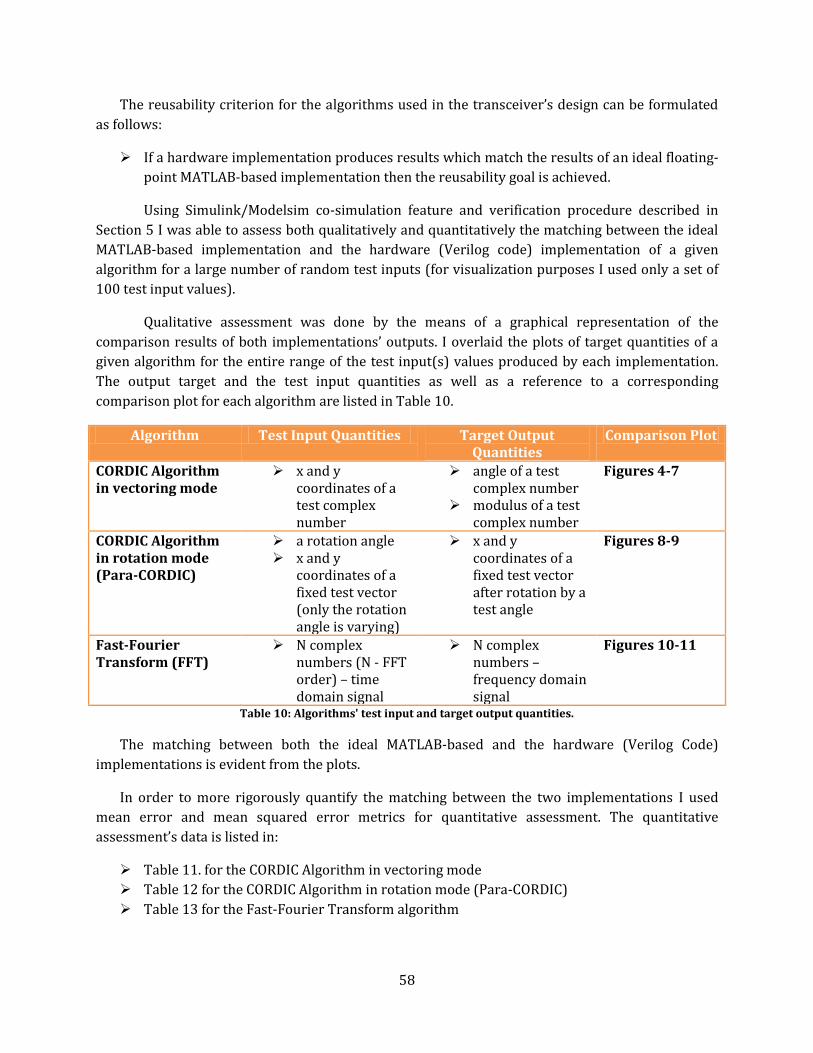
58
The reusability criterion for the algorithms used in the transceiver’s design can be formulated
as follows:
If a hardware implementation produces results which match the results of an ideal floating-
point MATLAB-based implementation then the reusability goal is achieved.
Using Simulink/Modelsim co-simulation feature and verification procedure described in
Section 5 I was able to assess both qualitatively and quantitatively the matching between the ideal
MATLAB-based implementation and the hardware (Verilog code) implementation of a given
algorithm for a large number of random test inputs (for visualization purposes I used only a set of
100 test input values).
Qualitative assessment was done by the means of a graphical representation of the
comparison results of both implementations’ outputs. I overlaid the plots of target quantities of a
given algorithm for the entire range of the test input(s) values produced by each implementation.
The output target and the test input quantities as well as a reference to a corresponding
comparison plot for each algorithm are listed in Table 10.
Algorithm Test Input Quantities Target Output Quantities
Comparison Plot
CORDIC Algorithm in vectoring mode
x and y coordinates of a test complex number
angle of a test complex number
modulus of a test complex number
Figures 4-7
CORDIC Algorithm in rotation mode (Para-CORDIC)
a rotation angle x and y
coordinates of a fixed test vector (only the rotation angle is varying)
x and y coordinates of a fixed test vector after rotation by a test angle
Figures 8-9
Fast-Fourier Transform (FFT)
N complex numbers (N - FFT order) – time domain signal
N complex numbers – frequency domain signal
Figures 10-11
Table 10: Algorithms' test input and target output quantities.
The matching between both the ideal MATLAB-based and the hardware (Verilog Code)
implementations is evident from the plots.
In order to more rigorously quantify the matching between the two implementations I used
mean error and mean squared error metrics for quantitative assessment. The quantitative
assessment’s data is listed in:
Table 11. for the CORDIC Algorithm in vectoring mode
Table 12 for the CORDIC Algorithm in rotation mode (Para-CORDIC)
Table 13 for the Fast-Fourier Transform algorithm

59
If a given algorithm’s output was computed by the means of one operation the matching
condition would be explicitly stated in terms of the error’s magnitude with respect to input bit
precision. In that case the condition for a match would be that the error is less than the smallest
representable number in the input’s fixed-point representation. Due to the fact that all test input
signals are represented in 8.8 fixed-point representation (8 bits for the integer part and 8 bits for
the fractional part) the error should be less than 2-8= 0.0039.
However, none of the algorithms is computed in one step and truncation effect occurring in
the intermediate stages requires complicated numerical analysis to determine the error’s upper
bound. Unfortunately, such an analysis is beyond the scope of this project.
Nevertheless, the mean error values and the mean squared error values for each algorithm
are close to the error’s lower bound for one-step operation and it can be concluded that the
hardware implementation of the algorithms matches the ideal floating-point MATLAB- based
implementation in terms of functionality. Therefore the reusability condition set for the hardware
implementation of the algorithms is met.
Figure 4: The overlaid angle results (100 test input values) for both the floating-point MATLAB-based and the
hardware (Verilog code) implementations of the CORDIC algorithm in vectoring mode.
0 20 40 60 80 100 1200
0.2
0.4
0.6
0.8
1
1.2
1.4
1.6
Input Test Set Index
An
gle
Angle (Floating-point MATLAB function)
Angle (Hardware Verilog Code)

60
Figure 5: The difference in the angle results (100 test input values) between the floating-point MATLAB-based
and the hardware (Verilog code) implementations of the CORDIC algorithm in vectoring mode.
Figure 6: The overlaid modulus results for both the floating-point MATLAB-based and the hardware (Verilog
code) implementations of the CORDIC algorithm in vectoring mode.
0 20 40 60 80 100 120-4
-2
0
2
4
6
8
10
12
14x 10
-3
Input Test Set Index
Diffe
ren
ce
Difference between floating-point MATLAB function and hardware Verilog angle outputs
0 20 40 60 80 100 1200
2
4
6
8
10
12
14
Input Test Set Index
Mo
du
lus
Modulus (Floating-point MATLAB function)
Modulus (Hardware Verilog Code))

61
Figure 7: The difference in the modulus results (100 test input values) between the floating-point MATLAB-based
and the hardware (Verilog code) implementations of the CORDIC algorithm in vectoring mode.
Target Output Quantity
CORDIC Algorithm In Vectoring Mode Difference Between The Floating-Point MATLAB-based Implementation And The Hardware (Verilog Code) Implementation Hardware 16-bit Fixed-point Representation
Mean Error Mean Squared Error
Input Output (angle/modulus)
Integer Part
Fractional Part
Integer Part
Fractional Part
Angle 8 bits 8 bits 3 13 0.0010 1.0577x10⁻⁶
Modulus 8 bits 8 bits 8 8 0.0172 2.9493x10⁻⁴
Table 11: The difference between the floating-Point MATLAB-based implementation and the Hardware (Verilog
Code) implementation of the CORDIC algorithm in vectoring mode.
0 20 40 60 80 100 120-0.02
-0.01
0
0.01
0.02
0.03
0.04
0.05
0.06
Input Test Set Index
Diffe
ren
ce
Difference between floating-point MATLAB function and hardware Verilog modulus outputs

62
Figure 8: The overlaid rotated x and y coordinates' results (100 test input values) for both the floating-point
MATLAB-based and the hardware (Verilog code) implementations of the CORDIC algorithm in rotation mode
(Para-CORDIC).
Figure 9: The difference in the rotated x and y coordinates' results (100 test input values) between the floating-
point MATLAB-based and the hardware (Verilog code) implementations of the CORDIC algorithm in rotation
mode (Para-CORDIC).
0 0.1 0.2 0.3 0.4 0.5 0.6 0.7 0.8 0.9 1-0.8
-0.6
-0.4
-0.2
0
0.2
0.4
0.6
0.8
Normalized to 2pi Rotation Angle In Radians
Am
plit
ud
e
0 0.1 0.2 0.3 0.4 0.5 0.6 0.7 0.8 0.9 1-0.8
-0.6
-0.4
-0.2
0
0.2
0.4
0.6
0.8
Normalized to 2pi Rotation Angle In Radians
Am
plit
ud
e
Rotated vector's x coordinate (Floating-point MATLAB function)
Rotated vector's x coordinate (Hardware Verilog Code)
Rotated vector's y coordinate (Floating-point MATLAB function)
Rotated vector's x coordinate (Hardware Verilog Code)
0 0.1 0.2 0.3 0.4 0.5 0.6 0.7 0.8 0.9 1-0.03
-0.02
-0.01
0
0.01
0.02
0.03
Normalized to 2pi Rotation Angle In Radians
Diffe
ren
ce
0 0.1 0.2 0.3 0.4 0.5 0.6 0.7 0.8 0.9 1-0.03
-0.02
-0.01
0
0.01
0.02
0.03
Normalized to 2pi Rotation Angle In Radians
Diffe
ren
ce
Difference between floating-point MATLAB function and hardware Verilog rotated vector's x coordinate
Difference between floating-point MATLAB function and hardware Verilog rotated vector's y coordinate
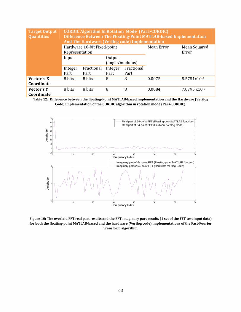
63
Target Output Quantities
CORDIC Algorithm In Rotation Mode (Para-CORDIC) Difference Between The Floating-Point MATLAB-based Implementation And The Hardware (Verilog code) Implementation
Hardware 16-bit Fixed-point Representation
Mean Error Mean Squared Error
Input Output (angle/modulus)
Integer Part
Fractional Part
Integer Part
Fractional Part
Vector’s X Coordinate
8 bits 8 bits 8 8 0.0075 5.5751x10⁻⁵
Vector’s Y Coordinate
8 bits 8 bits 8 8 0.0084 7.0795 x10⁻⁵
Table 12: Difference between the floating-Point MATLAB-based implementation and the Hardware (Verilog
Code) implementation of the CORDIC algorithm in rotation mode (Para-CORDIC).
Figure 10: The overlaid FFT real part results and the FFT imaginary part results (1 set of the FFT test input data)
for both the floating-point MATLAB-based and the hardware (Verilog code) implementations of the Fast-Fourier
Transform algorithm.
0 10 20 30 40 50 60 70-10
0
10
20
30
40
50
60
70
Frequency Index
Am
plit
ud
e
Real part of 64-point FFT (Floating-point MATLAB function)
Real part of 64-point FFT (Hardware Verilog Code)
0 10 20 30 40 50 60 70-5
0
5
Frequency Index
Am
plit
ud
e
Imaginary part of 64-point FFT (Floating-point MATLAB function)
Imaginary part of 64-point FFT (Hardware Verilog Code)

64
Figure 11: The difference in the FFT real part results and the FFT imaginary part results (1 set of the FFT test
input data) for both the floating-point MATLAB-based and the hardware (Verilog code) implementations of the
Fast-Fourier Transform algorithm.
Target Output Quantity
Fast-Fourier Transform (FFT) Difference Between The Floating-Point MATLAB-based Implementation And The Hardware (Verilog code) Implementation
Hardware 16-bit Fixed-point Representation
Mean Error Mean Squared Error
Input Output (angle/modulus)
Integer Part
Fractional Part
Integer Part
Fractional Part
FFT Real Part 8 bits 8 bits 8 8 0.0154 2.3811x10⁻⁴
FFT Imaginary Part
8 bits 8 bits 8 8 0.0141 1.9822 x10⁻⁴
Table 13: Difference between the floating-Point MATLAB-based implementation and the Hardware (Verilog
Code) implementation of the Fast-Fourier Transform algorithm.
6.2 RESULTS FOR ASSESSMENT OF REUSABILITY OF THE OFDM TRANSCEIVER
The assessment of reusability of the entire system was realized through evaluation of the
transceiver’s ability to estimate and compensate for synchronization errors which is reflected in
error-free decoding of the transmitted data symbols in various channel conditions.
0 10 20 30 40 50 60 70-0.05
0
0.05
0.1
0.15
Frequency Index
Diffe
ren
ce
Difference between floating-point MATLAB function and hardware Verilog FFT's real parts
0 10 20 30 40 50 60 70-0.06
-0.04
-0.02
0
0.02
0.04
0.06
0.08
Frequency Index
Diffe
ren
ce
Difference between floating-point MATLAB function and hardware Verilog FFT's imaginary parts

65
I tested the transceiver in channels of a varying degree of the multipath effect. The
multipath effect is determined by the number of coefficients and their relative magnitudes with
respect to the line-of-sight component (the first coefficient in the channel impulse response) in the
channel impulse response. The more the terms in the channel impulse response the more the
copies of the transmitted signal with various delays corresponding to the coefficients’ positions in
the channel impulse response are being combined at the receiver. Severity of the negative effect on
decoding of the resulting superposition of signals depends on how close in magnitude the copies
are with respect to the earliest component (the line-of-sight component). If the coefficients in the
channel impulse response constitute a significant percentage of the line-of-sight component’s
magnitude then distinctive features of the underlying analog signal which differentiate the
transmitted data symbols are lost (due to the “smearing” effect of the overlapping copies) and as a
result, more detection errors occur.
The channels (in increasing degree of the multipath effect) used in evaluation of the
system’s robustness to synchronization errors are:
ideal channel – impulse response h=[1 0]
mild multipath channel – impulse response h=[1 0.1 0.05 0.002 0.001]
severe multipath channel - impulse response h=[0.8 0.2 0.1 0.05 0.02]
I used a similar approach as in the case of algorithms’ hardware implementation evaluation.
The proof of meeting the reusability condition set for the transceiver was obtained both through
qualitative (graphical representation) and quantitative (numerical metrics) assessment. The
qualitative evaluation consists of a graphical representation of a comparison of the transmitted and
the decoded data symbols (Appendix Section 8.2.1 Figure 17, Appendix Section 8.2.2 Figure 21 and
Appendix Section 8.2.3 Figure 25), their difference (Appendix Section 8.2.1 Figure 18, Appendix
Section 8.2.2 Figure 22 and Appendix Section 8.2.3 Figure 26) and the mapping of the decoded
symbols onto 16-QAM constellation (Appendix Section 8.2.1 Figure 19, Appendix Section 8.2.2
Figure 23 and Appendix Section 8.2.3 Figure 27). The quantitative evaluation consists of the
following numerical metrics (Appendix Section 8.2.1 Table 15, Appendix Section 8.2.2 Table 16 and
Appendix Section 8.2.3 Table 17):
symbol error rate – indicates how many symbols were decoded in error out of all
transmitted symbols. It quantifies the composite effect of errors on both in-phase (real
part) and quadrature (imaginary part) components of the data 16-QAM symbol.
mean error and mean squared error of the real and the imaginary parts of the data
symbols – quantifies an error along each axis in the 16-QAM source symbol constellation
diagram.
As can be seen from both the graphical representation of the comparison results and the
numerical results in both the ideal and the mild multipath channels the transceiver achieves
perfect decoding – no errors. In the case of severe multipath channel the results are also
promising. The transceiver achieves almost perfect decoding (symbol error rate is only 1.95%). It
has to be pointed out that the errors which occurred in the case of transmission through the
severe multipath channel are not resulting from the transceiver structure. There errors are

66
inherent to the channel distortion of the transmitted signal (the “smearing” effect in severe
multipath channels). The “smearing” effect can be observed in the plots illustrating the timing
offset metric for the first synchronization preamble (Preamble 1). Due to the “smearing” effect the
area of the first autocorrelation peak (the region affected the most by the delay spread of the
multipath channel)in the case of the severe multipath channel is populated with a larger number
of erroneous peaks than in the case of the ideal or the mild multipath channels. As can be seen in
Appendix Section 8.2.3 Figure 28 the magnitude of erroneous peaks approaches the magnitude of
the actual first autocorrelation peak. In the corresponding plots (Appendix Section 8.2.1 Figure 20
and Appendix Section 8.2.2 Figure 24) for the ideal and the mild multipath channels there is a
distinct peak corresponding to the true autocorrelation peak and it is surrounded by fewer and
most importantly, much smaller erroneous peaks. The smearing effect can also be observed in the
plots illustrating the mapping of the decoded data symbols on the 16-QAM constellation (Appendix
Section 8.2.1 Figure 19, Appendix Section 8.2.2 Figure 23 and Appendix Section 8.2.3 Figure 27).
The higher the severity of the multipath effect the thicker the dots comprised of the overlaid data
symbols (prior to the 16-QAM de-mapper) around 16-QAM constellation points are. However, in
all three cases (ideal, mild and severe multipath channels) all data symbols are kept within each
constellation point’s decision region therefore a perfect decoding (and in the case of the severe
channel close to perfect) has been achieved.
In Tables - Appendix Section 8.2.1 Table 15, Appendix Section 8.2.2 Table 16 and Appendix
Section 8.2.3 Table 17 there is included information about the effectiveness of estimation of the
frequency offset. As can be seen from the total estimate values (combined coarse and fine
synchronization estimates which are also listed separately in the tables) the transceiver accurately
estimates the fractional frequency offset in all three test cases. Tiny discrepancies between the
actual frequency offset value and the estimates in the case of the mild and the severe multipath
channels (4.133 % difference for the mild multipath channel and 6.933% difference for the severe
multipath channel) result from the fact that distortion caused by the multipath effect (the
smearing effect) affects also synchronization information enclosed in the transmitted symbols
(thumb-tack autocorrelation property of a PN sequence, conjugate symmetry of the preambles).
Since the synchronization mechanism by no means can predict what happened during the
transmission and revert the changes made by the channel the loss in synchronization information
is reflected in accuracy of estimates. Nevertheless, the robustness of the synchronization
mechanism in spite of distortion caused by the smearing effect is evident from closeness of the
estimates to the actual value of the frequency offset in all degrees of severity of the multipath
effect.
I also simulated the effects of synchronization errors by disabling the synchronization
mechanism. I considered each synchronization error separately and also their combined effect. I
used the same graphical and numerical representations of the assessment data as in the case of the
transceiver’s performance testing in various multipath channels. Table 14 lists all the considered
cases of synchronization errors along with the references to each case’s graphical and numerical
representations of the assessment data.

67
Case Assessment Data
Graphical Representation Numerical Representation
Ideal channel with an uncompensated frequency offset
Appendix Section 8.2.4 Figures 29-31
Appendix Section 8.2.4 Table 18
Ideal channel with a symbol timing offset (FFT window leads)
Appendix Section 8.2.5 Figures 32-34
Appendix Section 8.2.5 Table 19
Ideal channel with a symbol timing offset (FFT window lags)
Appendix Section 8.2.6 Figures 35-37
Appendix Section 8.2.6 Table 20
Ideal channel with both a symbol timing offset (FFT windows leads) and an uncompensated frequency offset
Appendix Section 8.2.7 Figures 38-40
Appendix Section 8.2.7 Table 21
Table 14: The list of the simulated cases of synchronization errors and the references to their assessment data.
Through the results illustrating the effect of each synchronization error I gained a valuable
insight into importance of the fundamental principle of the OFDM modulation – orthogonality
principle between OFDM subcarriers. The results obtained convinced me of necessity of a perfect
synchronization in the case of OFDM-based receivers. As can be seen from the plots and the
performance metrics, such as symbol error rate, OFDM demodulation is extremely sensitive to
synchronization impairments. Even small synchronization errors cause loss of orthogonality
between subcarriers and in effect completely deteriorate performance of the OFDM receiver
rendering it useless for any serious applications – the symbol error rate ranges from 0.54 to 0.80.
As can be seen in Appendix Section 8.2.4 Figure 31, Appendix Section 8.2.5 Figure 34,
Appendix Section 8.2.6 Figure 37 and Appendix Section 8.2.7 Figure 40 the consequence of the loss
of orthogonality between subcarriers is the scattering effect of the decoded data symbols
throughout the decision regions of the 16-QAM constellation points and as a result decoding of the
“garbage” data.
Moreover, from a comparison of the separate and combined effects of the synchronization
errors it can be concluded that a single synchronization error introduces such a large error floor
that it really does not matter whether the system fails in only one synchronization error
detection/correction or all of them due to the fact that in all of the cases the resulting performance
is at an unacceptable level for any sort of applications.
As can be concluded from the results the transceiver is robust to various synchronization
errors. It correctly estimates synchronization errors and compensates for them which ultimately
leads to error-free decoding of the source data symbols.
7 CONCLUSION

68
Taking into account diversity of disparate communication theory and hardware
implementation concepts employed in the OFDM transceiver design I consider this project as an
ideal culminating design experience for my final year as a M. Eng student.
I exercised both the roles of a system engineer and a hardware engineer in realization of the
project which provided me with invaluable experience highly sought in a professional engineering
environment. I succeeded in both of the roles as the overall system and the hardware
implementation of various algorithms met the desired expectations. A comparison to the reference
system – 802.11a modem on which the transceiver’s parameters were based yields promising
results. I managed to design synchronization mechanism using only two preambles (2 64-sample
long preambles for fine and coarse synchronization) as opposed to five preambles used in 802.11a
standard (3 16-sample long short preambles for coarse synchronization and 2 64-sample long
preambles for fine synchronization). In addition to that, by implementing the fastest available
variations of algorithms used in construction of the OFDM transceiver the higher data rates can be
achieved than in the case of 802.11a modems. I design the system for 27 MHz sampling clock rate
(one of the oscillators’ frequency in Altera Cyclone II FPGA) whereas in 802.11a modems 20 MHz
sampling frequency is used.
The main goal of the project – reusability of the project’s materials by students with similar
interest and background in communication theory and digital hardware was achieved by
verification of the system’s functionality.
The possibility of reusing my design by students to supplement their communication
systems’ study outside the classroom made the OFDM transceiver design an appropriate choice for
my M. Eng project.
REFERENCES
[1] Byungjoon Park, Hyunsoo Cheon, Changeon Kang, Daesik Hong. “A simple preamble for
OFDM timing offset estimation.” Vehicular Technology Conference, 2002. Proceedings. VTC. Vol. 2.
2002: 729 - 732
[2] Chiueh, Tzi-Dar, and Per-Yun Tsai. OFDM Baseband Receiver Design for Wireless
Communications. 1st ed. : Wiley, 2007
[3] De Caro, D., N. Petra, A. G. M. Strollo. “A 380 MHz Direct Digital Synthesizer/Mixer With
Hybrid CORDIC Architecture in 0.25 µm CMOS”. Solid-State Circuits, IEEE Journal. Issue 1. 2007:
151-160
[4] Fazel, Khaled, and Stefan Kaiser. Multi-Carrier and Spread Spectrum Systems: From OFDM
and MC-CDMA to LTE and WiMAX. 2nd ed. : Wiley, 2008
69
[5] Juang, Tso-Bing, Hsiao Shen-Fu, Tsai Ming-Yu. “Para-CORDIC: parallel CORDIC rotation
algorithm.” Circuits and Systems I: Regular Papers. Volume 51. Issue 8. 2004: 1515 - 1524
[6] Maharatna, Koushik, Eckhard Grass, and Ulrich Jagdhold. A 64-Point Fourier Transform
Chip for High-Speed
[7] Meyer-Baese , Uwe. Digital Signal Processing with Field Programmable Gate Arrays (Signals
and Communication Technology). 3rd ed. : Springer, 2007
[8] Minn, H.; M. Zeng, V.K. Bhargava. “On timing offset estimation for OFDM systems.”
Communications Letters, IEEE. Vol. 4. Issue 7. 2000: 242 - 244
[9] Muller, Jean-Michel. Elementary Functions: Algorithms and Implementation. 2nd ed. :
Birkhäuser Boston, 2005
[10] Osorio, R.R., E. Antelo, J.D. Bruguera, J. Villalba, E.L. Zapata. “Digit on-line large radix CORDIC
rotator.” Application Specific Array Processors. 1995: 246 - 257
[11] Schmidl, T.M., D.C. Cox. “Robust frequency and timing synchronization for OFDM.”
Communications, IEEE. Vol. 45. Issue 12. 1997: 1613 - 1621
[12] Torosyan, A., Fu Dengwei, A.N., Jr. Willson. “A 300 MHz quadrature direct digital
synthesizer/mixer in 0.25 µm CMOS.” Solid-State Circuits Conference, 2002. Digest of Technical
Papers. ISSCC. 2002 IEEE International. Vol. 1. 2002: 132 - 133
[13] Villalba, J., J.C. Arrabal, E.L. Zapata, E. Antelo, J.D Bruguera. “Radix-4 vectoring CORDIC
algorithm and architectures.” Application Specific Systems, Architectures and Processors 1996.
ASAP 96. 1996: 55 - 64
[14] Wang , Qiang, Cheng Tao, Wei Huang. “Efficient Implementation of Synchronization in
OFDM System Based on FPGA.” Advanced Communication Technology. Vol. 1. 2007: 178 - 181

70
8 APPENDIX
8.1 CIRCUIT DIAGRAMS
Figure 12: Circuit diagram of the OFDM receiver.
COARSE SYNCHRONIZATION
FINE SYNCHRONIZATION
EQUALIZATION/DATA DECODING CHANNEL ESTIMATION

71
Figure 13: Circuit diagram of the Coarse Frequency Offset Metric Calculation Unit - serial multiplier/accumulator mechanism.

72
Figure 14: Circuit diagram of the Fine Frequency Offset Metric Calculation Unit.

73
Figure 15: Circuit diagram of the Clipped Cross-correlator Unit.

74
Figure 16: Circuit diagram of the Para-CORDIC based de-rotator.
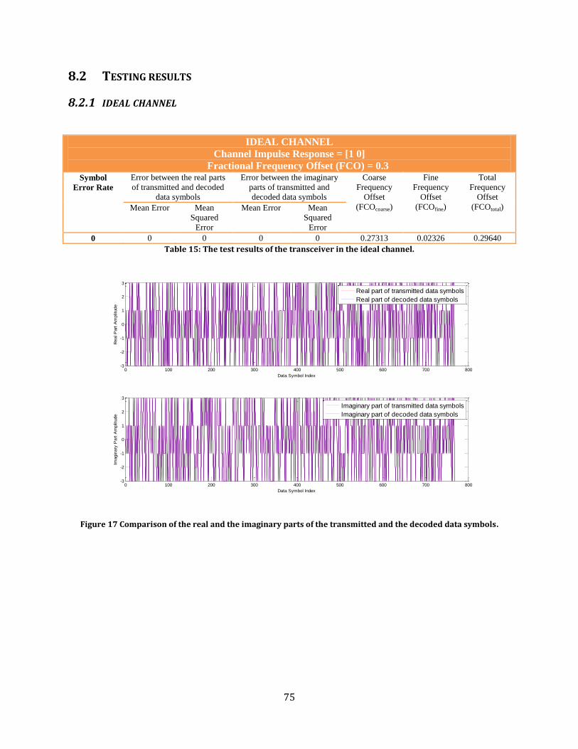
75
8.2 TESTING RESULTS
8.2.1 IDEAL CHANNEL
IDEAL CHANNEL
Channel Impulse Response = [1 0]
Fractional Frequency Offset (FCO) = 0.3 Symbol
Error Rate
Error between the real parts
of transmitted and decoded
data symbols
Error between the imaginary
parts of transmitted and
decoded data symbols
Coarse
Frequency
Offset
(FCOcoarse)
Fine
Frequency
Offset
(FCOfine)
Total
Frequency
Offset
(FCOtotal) Mean Error Mean
Squared
Error
Mean Error Mean
Squared
Error
0 0 0 0 0 0.27313 0.02326 0.29640
Table 15: The test results of the transceiver in the ideal channel.
Figure 17 Comparison of the real and the imaginary parts of the transmitted and the decoded data symbols.
0 100 200 300 400 500 600 700 800-3
-2
-1
0
1
2
3
Data Symbol Index
Real P
art
Am
plit
ude
0 100 200 300 400 500 600 700 800-3
-2
-1
0
1
2
3
Data Symbol Index
Imagin
ary
Part
Am
plit
ude
Real part of transmitted data symbols
Real part of decoded data symbols
Imaginary part of transmitted data symbols
Imaginary part of decoded data symbols
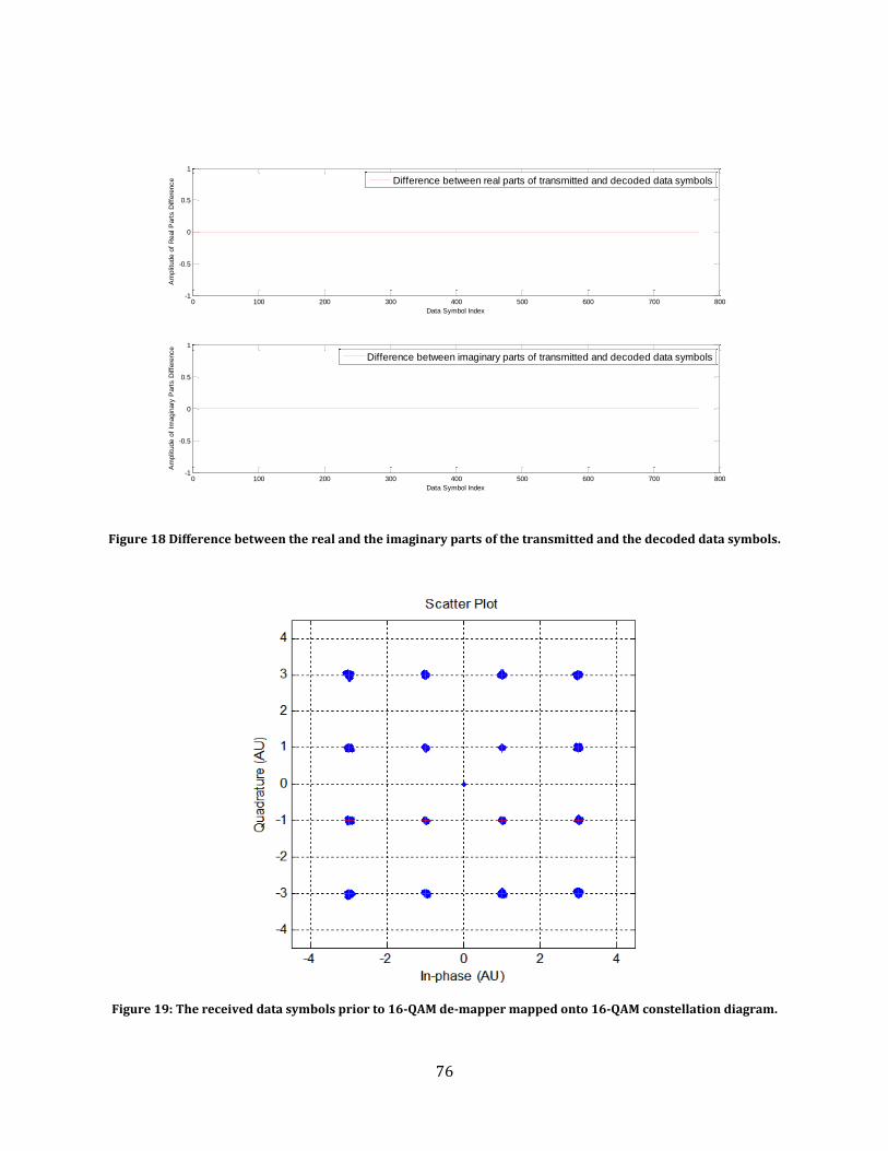
76
Figure 18 Difference between the real and the imaginary parts of the transmitted and the decoded data symbols.
Figure 19: The received data symbols prior to 16-QAM de-mapper mapped onto 16-QAM constellation diagram.
0 100 200 300 400 500 600 700 800-1
-0.5
0
0.5
1
Data Symbol Index
Am
plit
ude o
f R
eal P
art
s D
iffe
rence
0 100 200 300 400 500 600 700 800-1
-0.5
0
0.5
1
Data Symbol Index
Am
plit
ude o
f Im
agin
ary
Part
s D
iffe
rence
Difference between real parts of transmitted and decoded data symbols
Difference between imaginary parts of transmitted and decoded data symbols

77
Figure 20: Timing Offset Metric for the Preamble 1.
8.2.2 MILD MULTI-PATH CHANNEL
MILD MULTT-PATH CHANNEL
Channel Impulse Response = [1 0.1 0.05 0.002 0.001]
Fractional Frequency Offset (FCO) = 0.3 Symbol Error
Rate
Error between the real parts
of transmitted and decoded
data symbols
Error between the
imaginary parts of
transmitted and decoded
data symbols
Coarse
Frequency
Offset
(FCOcoarse)
Fine
Frequency
Offset
(FCOfine)
Total
Frequency
Offset
(FCOtotal)
Mean Error Mean
Squared
Error
Mean Error Mean
Squared
Error
𝟎
𝟕𝟔𝟗= 𝟎
0 0 0 0 0.2728 0.0148 0.2876
Table 16: The test results of the transceiver in the mild multipath channel.
0 10 20 30 40 50 60 70 80 900
1
2
3
4
5
6
Clock cycle
Tim
ing O
ffset
Metr
ic M
agnitude
Timing offset metric for the preamble 1
Autocorrelation threshold
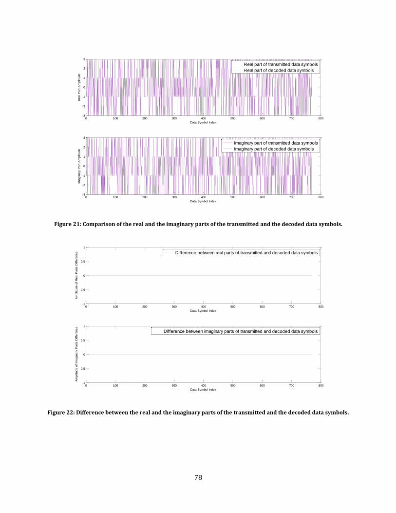
78
Figure 21: Comparison of the real and the imaginary parts of the transmitted and the decoded data symbols.
Figure 22: Difference between the real and the imaginary parts of the transmitted and the decoded data symbols.
0 100 200 300 400 500 600 700 800-3
-2
-1
0
1
2
3
Data Symbol Index
Real P
art
Am
plit
ude
Real part of transmitted data symbols
Real part of decoded data symbols
0 100 200 300 400 500 600 700 800-3
-2
-1
0
1
2
3
Data Symbol Index
Imagin
ary
Part
Am
plit
ude
Imaginary part of transmitted data symbols
Imaginary part of decoded data symbols
0 100 200 300 400 500 600 700 800-1
-0.5
0
0.5
1
Data Symbol Index
Am
plit
ude o
f R
eal P
art
s D
iffe
rence
Difference between real parts of transmitted and decoded data symbols
0 100 200 300 400 500 600 700 800-1
-0.5
0
0.5
1
Data Symbol Index
Am
plit
ude o
f Im
agin
ary
Part
s D
iffe
rence
Difference between imaginary parts of transmitted and decoded data symbols

79
Figure 23: The received data symbols prior to 16-QAM de-mapper mapped onto 16-QAM constellation diagram.
Figure 24: Timing Offset Metric for the Preamble 1.
0 10 20 30 40 50 60 70 80 900
1
2
3
4
5
6
Clock cycle
Tim
ing O
ffset
Metr
ic M
agnitude
Timing offset metric for the preamble 1
Autocorrelation threshold

80
8.2.3 SEVERE MULTI-PATH CHANNEL
SEVERE MULTT-PATH CHANNEL
Channel Impulse Response = [0.8 0.2 0.1 0.05 0.02]
Fractional Frequency Offset (FCO) = 0.3 Symbol Error
Rate
Error between the real parts of
transmitted and decoded data
symbols
Error between the
imaginary parts of
transmitted and decoded
data symbols
Coarse
Frequency
Offset
(FCOcoarse)
Fine
Frequency
Offset
(FCOfine)
Total
Frequency
Offset
(FCOtotal)
Mean
Error
Mean Squared
Error
Mean
Error
Mean
Squared
Error
𝟏𝟓
𝟕𝟔𝟗= 𝟎.𝟎𝟏𝟗𝟓
0.0078 6.0877x10⁻⁵ 0.0117 1.3697 x10⁻⁴ 0.2660 0.0131 0.2792
Table 17: The test results of the transceiver in the severe multipath channel.
Figure 25: Comparison of the real and the imaginary parts of the transmitted and the decoded data symbols.
0 100 200 300 400 500 600 700 800-3
-2
-1
0
1
2
3
Data Symbol Index
Real P
art
Am
plit
ude
Real part of transmitted data symbols
Real part of decoded data symbols
0 100 200 300 400 500 600 700 800-3
-2
-1
0
1
2
3
Data Symbol Index
Imagin
ary
Part
Am
plit
ude
Imaginary part of transmitted data symbols
Imaginary part of decoded data symbols

81
Figure 26: Difference between the real and the imaginary parts of the transmitted and the decoded data symbols.
Figure 27: The received data symbols prior to 16-QAM de-mapper mapped onto 16-QAM constellation diagram.
0 100 200 300 400 500 600 700 800-2
-1.5
-1
-0.5
0
0.5
1
1.5
2
Data Symbol Index
Am
plit
ude o
f R
eal P
art
s D
iffe
rence
Difference between real parts of transmitted and decoded data symbols
0 100 200 300 400 500 600 700 800-2
-1.5
-1
-0.5
0
0.5
1
1.5
2
Data Symbol Index
Am
plit
ude o
f Im
agin
ary
Part
s D
iffe
rence
Difference between imaginary parts of transmitted and decoded data symbols

82
Figure 28: Timing Offset Metric for the Preamble 1.
8.2.4 IDEAL CHANNEL WITH AN UNCOMPENSATED FREQUENCY OFFSET
IDEAL CHANNEL WITH AN UNCOMPENSTAD FREQUECY OFFSET
Channel Impulse Response = [1 0]
Fractional Frequency Offset (FCO) = 0.3
Symbol Error
Rate
Error between the real parts
of transmitted and decoded
data symbols
Error between the
imaginary parts of
transmitted and decoded
data symbols
Coarse
Frequency
Offset
(FCOcoarse)
Fine
Frequency
Offset
(FCOfine)
Total
Frequency
Offset
(FCOtotal)
Mean Error Mean
Squared
Error
Mean Error Mean
Squared
Error
𝟓𝟕𝟔
𝟕𝟔𝟗= 𝟎.𝟕𝟒𝟗𝟎
0.5085 0.2585 0.5020 0.2520 N/A N/A N/A
Table 18: The test results of the transceiver in the ideal channel with an uncompensated frequency offset - the
frequency offset synchronization mechanism is disabled.
0 10 20 30 40 50 60 70 80 900
2
4
6
8
10
12
14
Clock cycle
Tim
ing O
ffset
Metr
ic M
agnitude
Timing offset metric for the preamble 1
Autocorrelation threshold

83
Figure 29: Comparison of the real and the imaginary parts of the transmitted and the decoded data symbols.
Figure 30: Difference between the real and the imaginary parts of the transmitted and the decoded data symbols.
0 100 200 300 400 500 600 700 800-3
-2
-1
0
1
2
3
Data Symbol Index
Real P
art
Am
plit
ude
0 100 200 300 400 500 600 700 800-3
-2
-1
0
1
2
3
Data Symbol Index
Imagin
ary
Part
Am
plit
ude
Real part of transmitted data symbols
Real part of decoded data symbols
Imaginary part of transmitted data symbols
Imaginary part of decoded data symbols
0 100 200 300 400 500 600 700 800-6
-4
-2
0
2
4
6
Data Symbol Index
Am
plit
ude o
f R
eal P
art
s D
iffe
rence
Difference between real parts of transmitted and decoded data symbols
0 100 200 300 400 500 600 700 800-6
-4
-2
0
2
4
6
Data Symbol Index
Am
plit
ude o
f Im
agin
ary
Part
s D
iffe
rence
Difference between imaginary parts of transmitted and decoded data symbols

84
Figure 31: The received data symbols prior to 16-QAM de-mapper mapped onto 16-QAM constellation diagram.
8.2.5 IDEAL CHANNEL WITH A SYMBOL TIMING OFFSET (FFT WINDOW LEADS)
IDEAL CHANNEL WITH A SYMBOL TIMING OFFSET (FFT WINDOW LEADS)
Channel Impulse Response = [1 0]
Fractional Frequency Offset (FCO) = 0.3
Symbol timing offset = 4 (FFT window leads by 4 samples) Symbol Error
Rate
Error between the real parts
of transmitted and decoded
data symbols
Error between the
imaginary parts of
transmitted and decoded
data symbols
Coarse
Frequency
Offset
(FCOcoarse)
Fine
Frequency
Offset
(FCOfine)
Total
Frequency
Offset
(FCOtotal)
Mean Error Mean
Squared
Error
Mean Error Mean
Squared
Error
𝟒𝟏𝟐
𝟕𝟔𝟗= 𝟎.𝟓𝟑𝟓𝟖
0.2913 0.0848 0.3355 0.1126 0.2731 0.0043 0.2775
Table 19: The test results of the transceiver in the ideal channel with a symbol timing offset (FFT window leads) –
the symbol timing offset synchronization mechanism is disabled.

85
Figure 32: Comparison of the real and the imaginary parts of the transmitted and the decoded data symbols.
Figure 33: Difference between the real and the imaginary parts of the transmitted and the decoded data symbols.
0 100 200 300 400 500 600 700 800-3
-2
-1
0
1
2
3
Data Symbol Index
Real P
art
Am
plit
ude
Real part of transmitted data symbols
Real part of decoded data symbols
0 100 200 300 400 500 600 700 800-3
-2
-1
0
1
2
3
Data Symbol Index
Imagin
ary
Part
Am
plit
ude
Imaginary part of transmitted data symbols
Imaginary part of decoded data symbols
0 100 200 300 400 500 600 700 800-6
-4
-2
0
2
4
6
Data Symbol Index
Am
plit
ude o
f R
eal P
art
s D
iffe
rence
Difference between real parts of transmitted and decoded data symbols
0 100 200 300 400 500 600 700 800-6
-4
-2
0
2
4
6
Data Symbol Index
Am
plit
ude o
f Im
agin
ary
Part
s D
iffe
rence
Difference between imaginary parts of transmitted and decoded data symbols

86
Figure 34: The received data symbols prior to 16-QAM de-mapper mapped onto 16-QAM constellation diagram.
8.2.6 IDEAL CHANNEL WITH A SYMBOL TIMING OFFSET (FFT WINDOW LAGS)
IDEAL CHANNEL WITH A SYMBOL TIMING OFFSET (FFT WINDOW LAGS)
Channel Impulse Response = [1 0]
Fractional Frequency Offset (FCO) = 0.3
Symbol timing offset = 4 (FFT window lags by 4 samples) Symbol Error
Rate
Error between the real parts
of transmitted and decoded
data symbols
Error between the
imaginary parts of
transmitted and decoded
data symbols
Coarse
Frequency
Offset
(FCOcoarse)
Fine
Frequency
Offset
(FCOfine)
Total
Frequency
Offset
(FCOtotal)
Mean Error Mean
Squared
Error
Mean Error Mean
Squared
Error
𝟒𝟖𝟖
𝟕𝟔𝟗= 𝟎.𝟔𝟑𝟒𝟔
0.3979 0.1583 0.4174 0.1742 0.2731 -0.0568 0.2164
Table 20: The test results of the transceiver in the ideal channel with a symbol timing offset (FFT window lags) –
the symbol timing offset synchronization mechanism is disabled.

87
Figure 35: Comparison of the real and the imaginary parts of the transmitted and the decoded data symbols.
Figure 36: Difference between the real and the imaginary parts of the transmitted and the decoded data symbols.
0 100 200 300 400 500 600 700 800-3
-2
-1
0
1
2
3
Data Symbol Index
Real P
art
Am
plit
ude
0 100 200 300 400 500 600 700 800-3
-2
-1
0
1
2
3
Data Symbol Index
Imagin
ary
Part
Am
plit
ude
Real part of transmitted data symbols
Real part of decoded data symbols
Imaginary part of transmitted data symbols
Imaginary part of decoded data symbols
0 100 200 300 400 500 600 700 800-6
-4
-2
0
2
4
6
Data Symbol Index
Am
plit
ude o
f R
eal P
art
s D
iffe
rence
0 100 200 300 400 500 600 700 800-6
-4
-2
0
2
4
6
Data Symbol Index
Am
plit
ude o
f Im
agin
ary
Part
s D
iffe
rence
Difference between real parts of transmitted and decoded data symbols
Difference between imaginary parts of transmitted and decoded data symbols

88
Figure 37: The received data symbols prior to 16-QAM de-mapper mapped onto 16-QAM constellation diagram.
8.2.7 IDEAL CHANNEL WITH BOTH A SYMBOL TIMING OFFSET (FFT WINDOW LEADS) AND AN
UNCOMPENSATED FREQUENCY OFFSET
IDEAL CHANNEL WITH BOTH A SYMBOL TIMING OFFSET (FFT WINDOW LEADS)
AND AN UNCOMPENSATED FREQUENCY OFFSET
Channel Impulse Response = [1 0]
Fractional Frequency Offset (FCO) = 0.3
Symbol timing offset = 4 (FFT window leads by 4 samples) Symbol Error
Rate
Error between the real parts
of transmitted and decoded
data symbols
Error between the
imaginary parts of
transmitted and decoded
data symbols
Coarse
Frequency
Offset
(FCOcoarse)
Fine
Frequency
Offset
(FCOfine)
Total
Frequency
Offset
(FCOtotal)
Mean Error Mean
Squared
Error
Mean Error Mean
Squared
Error
𝟔𝟏𝟖
𝟕𝟔𝟗= 𝟎.𝟖𝟎𝟑𝟔
0.5241 0.2746 0.5800 0.3364 N/A N/A N/A
Table 21: The test results of the transceiver in the ideal channel with both a symbol timing offset (FFT window
leads) and an uncompensated frequency offset– the symbol timing offset and the frequency offset
synchronization mechanisms are disabled.
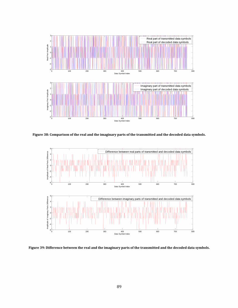
89
Figure 38: Comparison of the real and the imaginary parts of the transmitted and the decoded data symbols.
Figure 39: Difference between the real and the imaginary parts of the transmitted and the decoded data symbols.
0 100 200 300 400 500 600 700 800-3
-2
-1
0
1
2
3
Data Symbol Index
Real P
art
Am
plit
ude
Real part of transmitted data symbols
Real part of decoded data symbols
0 100 200 300 400 500 600 700 800-3
-2
-1
0
1
2
3
Data Symbol Index
Imagin
ary
Part
Am
plit
ude
Imaginary part of transmitted data symbols
Imaginary part of decoded data symbols
0 100 200 300 400 500 600 700 800-6
-4
-2
0
2
4
6
Data Symbol Index
Am
plit
ude o
f R
eal P
art
s D
iffe
rence
Difference between real parts of transmitted and decoded data symbols
0 100 200 300 400 500 600 700 800-6
-4
-2
0
2
4
6
Data Symbol Index
Am
plit
ude o
f Im
agin
ary
Part
s D
iffe
rence
Difference between imaginary parts of transmitted and decoded data symbols

90
Figure 40: The received data symbols prior to 16-QAM de-mapper mapped onto 16-QAM constellation diagram.