ORNL-TM-2009/100 Effective Size Analysis of the Diametral ...

ORNL-TM-2009/100

Effective Size Analysis of the Diametral Compression (Brazil) Test Specimen

Osama M. Jadaan College of Engineering, Mathematics, and Science

University of Wisconsin-Platteville Platteville, WI 53818 [email protected]

Andrew A. Wereszczak

Ceramic Science and Technology Group Materials Science and Technology Division

Oak Ridge National Laboratory Oak Ridge, TN 37831-6068

[email protected]

Publication Date: April 2009

Prepared by the OAK RIDGE NATIONAL LABORATORY

Oak Ridge, Tennessee 37831 managed by

UT-BATTELLE, LLC for the

U.S. DEPARTMENT OF ENERGY Under contract DE-AC05-00OR22725

ii

DOCUMENT AVAILABILITY Reports produced after January 1, 1996, are generally available free via the U.S. Department of Energy (DOE) Information Bridge:

Web site: http://www.osti.gov/bridge Reports produced before January 1, 1996, may be purchased by members of the public from the following source:

National Technical Information Service 5285 Port Royal Road Springfield, VA 22161 Telephone: 703-605-6000 (1-800-553-6847) TDD: 703-487-4639 Fax: 703-605-6900 E-mail: [email protected] Web site: http://www.ntis.gov/support/ordernowabout.htm

Reports are available to DOE employees, DOE contractors, Energy Technology Data Exchange (ETDE) representatives, and International Nuclear Information System (INIS) representatives from the following source:

Office of Scientific and Technical Information P.O. Box 62 Oak Ridge, TN 37831 Telephone: 865-576-8401 Fax: 865-576-5728 E-mail: [email protected] Web site: http://www.osti.gov/contact.html

This report was prepared as an account of work sponsored by an agency of the United States Government. Neither the United States government nor any agency thereof, nor any of their employees, makes any warranty, express or implied, or assumes any legal liability or responsibility for the accuracy, completeness, or usefulness of any information, apparatus, product, or process disclosed, or represents that its use would not infringe privately owned rights. Reference herein to any specific commercial product, process, or service by trade name, trademark, manufacturer, or otherwise, does not necessarily constitute or imply its endorsement, recommendation, or favoring by the United States Government or any agency thereof. The views and opinions of authors expressed herein do not necessarily state or reflect those of the United States Government or any agency thereof.

iii

TABLE OF CONTENTS

Page

LIST OF FIGURES ................................................................................................................ iv LIST OF TABLES .................................................................................................................. vi ABSTRACT ............................................................................................................................ 1 1. INTRODUCTION ......................................................................................................... 2 2. FLAT PUSH-ROD ........................................................................................................ 3 3. PUSH-ROD RADIUS OF CURVATURE > SPECIMEN RADIUS OF CURVATURE ............................................................................................................... 18 4. MATCHED RADII OF CURVATURE OF PUSH-ROD AND SPECIMEN .............. 28 5. RECOMMENDATIONS ............................................................................................... 38 6. ACKNOWLEDGEMENTS ........................................................................................... 38 7. REFERENCES .............................................................................................................. 39

iv

LIST OF FIGURES

Figure Page

1. Three loading configurations were examined. Flat push-rod (left). Push-rod radius of curvature greater than specimen radius of curvature (middle). Matched radii of curvature of push-rod and specimen (right). One-quarter symmetry of front view shown. Push rods are shown in gray, and the DC specimen is the sum of the blue and red portions. ...................................................... 3 2. Diametral compression (Brazil) test. Figure from Ref. [3]. ....................................... 3 3. DC specimen configuration and corresponding principal and shear stress distributions along the loading diametral direction [4]. .............................................. 4 4. Solid geometry for 1/8 symmetric model of the DC1 per Table I. ............................. 5

5. Regions under tensile and compressive normal stress in the DC specimen [5]. ......... 6 6. Mesh distribution for the 1/8 symmetric model of DC1 per Table I, having 30596 elements. .............................................................................................. 7 7. Maximum principal stress distribution (σ1) for DC1 of Figure 6. .............................. 8 8. Solid geometry for 1/8 symmetric model of the DC2. ................................................ 9 9. Mesh distribution for the 1/8 symmetric model of the DC2, having 74924 elements. ..................................................................................................................... 10 10. Maximum principal stress distribution (σ1) for DC2 of Fig. 8. .................................. 11 11. sx and sy distributions along the horizontal and vertical diametral directions (from [6]). ................................................................................................................... 12 12. Comparison between maximum principal stress distributions at mid-plane and side surface along the loading axis for DC1. Radial location = 0 is at the center of disk. ........................................................................................................ 13 13. Comparison between maximum principal stress distributions at mid-plane and side surface along the loading axis for DC2. Radial location = 0 is at the center of disk. ........................................................................................................ 13 14. Comparison between σz stress distributions across central thickness of DC1 and DC2. ..................................................................................................................... 15 15. Effective volume vs. Weibull modulus for the five DC specimens listed in Table I. ........................................................................................................................ 16 16. Effective area vs. Weibull modulus for the five DC specimens listed in Table I. ........................................................................................................................ 17 17. Maximum principal stress distribution (σ1) for DC 2 of Fig. 8 using WC push-rod instead of steel push-rod. ............................................................................. 18 18. Solid geometry for 1/8 symmetric model of the DC specimen. ................................. 20 19. Mesh distribution for the 1/8 symmetric model of the DC specimen. ........................ 21 20. Maximum principal stress distribution (σ1) for the DC specimen with steel curved end push-rod and no friction. .................................................................. 22 21. Maximum principal stress distribution (σ1) for the DC specimen with WC curved end push-rod and no friction. ................................................................... 23 22. Maximum principal stress distribution (σ1) for the DC specimen with curved end WC push-rod taking into account friction. ............................................... 24

v

Figure Page 23. Solid geometry for 1/8 symmetric model of the DC specimen with flat end push-rod. ..................................................................................................................... 25 24. Maximum principal stress distribution (σ1) for the DC specimen with flat end WC push-rod taking into account friction. ........................................................... 26 25. Effective volume vs. Weibull modulus for the DC specimens listed in Table III. ..... 27 26. Effective area vs. Weibull modulus for the DC specimens listed in Table III. .......... 27 27. Area and volume efficiencies as function of Weibull modulus for the DC specimen using WC curved end push-rod and taking friction into account. .............. 28 28. Solid geometry for 1/8 symmetric model of the DC specimen with 20° circular half-arc push-rod. The red sector makes 25° half-arc. ............................................... 29 29. Solid geometry for 1/8 symmetric model of the DC specimen with 40° circular half-arc push-rod. The red sector makes 45° half-arc. ............................................... 30 30. Mesh distribution for 1/8 symmetric model for the 20° half-arc DC specimen. ........ 31 31. Maximum principal stress distribution (σ1) for the DC specimen loaded with 20° circular half-arc WC push-rod and no friction. .................................................... 32 32. Maximum principal stress distribution (σ1) for the DC specimen loaded with 20° circular half-arc WC push-rod with friction. ........................................................ 33 33. Maximum principal stress distribution (σ1) for the DC specimen loaded with 40° circular half-arc WC push-rod and no friction. .................................................... 34 34. Maximum principal stress distribution (σ1) for the DC specimen loaded with 40° circular half-arc WC push-rod with friction. ........................................................ 35 35. Effect of push-rod arc-angle and friction on the maximum tensile stress in DC specimens. ........................................................................................................ 36 36. Effective volume vs. Weibull modulus for the DC specimens per Table V. .............. 37 37. Effective area vs. Weibull modulus for the DC specimens per Table V. ................... 38

vi

LIST OF TABLES

Table Page

I. Dimensions for the five DC specimens subjected to flat push-rod loading. ............... 6 II. Mechanical properties for ceramic and steel materials for flat push-rod FEA analysis. .............................................................................................................. 6 III. Simulation matrix for Section 3. ................................................................................. 19 IV. Mechanical properties for the ceramic specimen, WC, and steel materials used in Section 3. ................................................................................................................ 19 V. Simulation matrix for Section 4. ................................................................................. 30 VI. Mechanical properties for the ceramic specimen, WC, and steel materials used in Section 4. ................................................................................................................ 30

1

ABSTRACT

This study considers the finite element analysis (FEA) simulation and Weibull effective size analysis for the diametral compression (DC) or Brazil specimen loaded with three different push-rod geometries. Those geometries are a flat push-rod, a push-rod whose radius of curvature is larger than that for the DC specimen, and a push-rod whose radius of curvature matches that of the DC specimen. Such established effective size analysis recognizes that the tensile strength of structural ceramics is typically one to two orders of magnitude less than its compressive strength. Therefore, because fracture is much more apt to result from a tensile stress than a compressive one, this traditional analysis only considers the first principal tensile stress field in the mechanically loaded ceramic component for the effective size analysis. The effective areas and effective volumes were computed as a function of Weibull modulus using commercially available integrated design and reliability software. Particular attention was devoted to the effect of mesh sensitivity and localized stress concentration. The effect of specimen width on the stress state was also investigated. The effects of push-rod geometry, the use of steel versus tungsten carbide (WC) push-rods, and considering a frictionless versus no-slip interface between push-rod and specimen on the maximum stresses, where those stresses are located, and the effective area and effective volume results are described. Of the three push-rod geometries, it is concluded that the push-rod (made from WC rather than steel) whose radius of curvature matches that of the DC specimen is the most apt to cause fracture initiation within the specimen's bulk rather than at the loading interface. Therefore, its geometry is the most likely to produce a valid diametral compression strength test. However, the DC specimen remains inefficient in terms of its area and volume efficiencies; namely, the tensile strength of only a few percent of the specimen's entire area or volume is sampled. Given the high probability that a valid (or invalid) test can be proven by ceramic fractographic practices suggests that this test method and specimen is questionable for use with relatively strong structural ceramics.

2

1. INTRODUCTION The diametral compression (DC) or Brazil test can be used as an indirect measure of the tensile strength of a cylindrically-shaped specimen that is made from a brittle material (i.e., a material that has a low fracture toughness and who's uniaxial tensile strength is much less than its uniaxial compressive strength for the same volume of material). It is a test method developed in the early 1950s by two independent contemporaries [1-2]. It is a test now routinely used in rock and concrete mechanics as evidenced by there being an ASTM test method for it [3]. Interest has existed for quite some time to adapt this specimen geometry to structural ceramics. But several concerns exist. The tensile strengths of advanced ceramics are much higher than rock and concrete, so higher applied compressive forces or smaller specimens are needed to break or "split" the cylinder when it is diametrally and compressively loaded. This higher force introduces some complicating issues. The contact stresses can become extremely high before fracture commences (even with the use of interface cushions), this can result in cracking being initiated at the loading interfaces, and this cracking can cause fracture of the specimen or even "splitting". This scenario produces an invalid test and therefore needs to be avoided because the fixturing is essentially responsible for the fracture event and a (sought) bulk material response (i.e., tensile strength) is not sampled. Another concern is fractography is impracticle to use to confirm test validity (or invalidity). This is because failure force can be very high for strong ceramics, and the associated large amount of stored energy at fracture can fragment the specimen into a huge number of pieces (that assuredly undergo a lot of collateral damage among themselves during the event). So, at best, careful design of the DC specimen and loading platens can only increase the likelihood that a valid tensile strength of a structural ceramic can be generated; however, it cannot guarantee it. This report considers the finite element (FEA) simulation and Weibull effective size analysis for the DC or Brazil specimen loaded with three different push-rod geometries. Those geometries are a flat push-rod, a push-rod whose radius of curvature is larger than that for the DC specimen, and a push-rod whose radius of curvature matches that of the DC specimen. All three are respectively shown in Fig. 1. The very use of established effective size analysis recognizes that the tensile strength of structural ceramics is typically one to two orders of magnitude less than its compressive strength for the same amount of material. Therefore, because fracture is much more apt to result from a tensile stress than a compressive one, this traditional analysis only considers the first principal tensile stress field in the mechanically loaded ceramic component. The effective areas and effective volumes were computed as function of Weibull modulus using commercially available integrated design and reliability software (IDRS). Particular attention was devoted to the effect of mesh sensitivity and localized stress concentration. The effect of specimen width on the stress state was also investigated. The effects of push-rod geometry, the use of steel versus tungsten carbide (WC) push-rods, and considering a frictionless versus no-slip interface between push-rod and specimen on the maximum stresses, where those stresses are located, and the effective area and effective volume results are described.

3

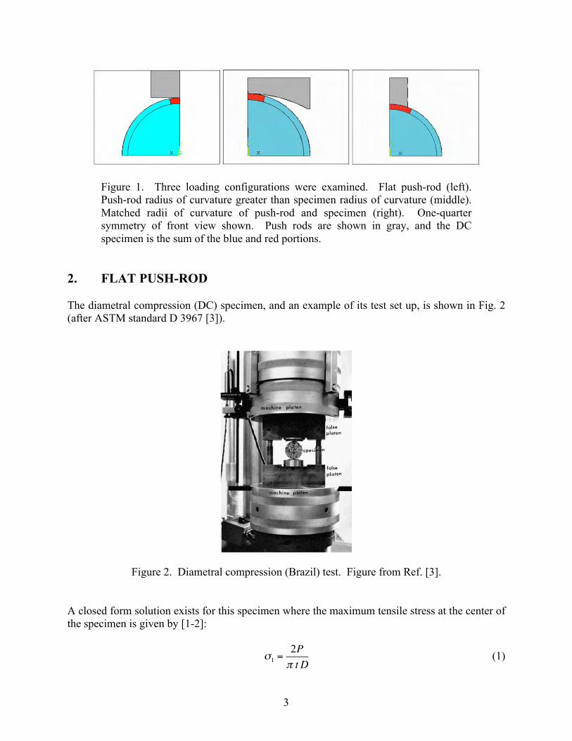
Figure 1. Three loading configurations were examined. Flat push-rod (left). Push-rod radius of curvature greater than specimen radius of curvature (middle). Matched radii of curvature of push-rod and specimen (right). One-quarter symmetry of front view shown. Push rods are shown in gray, and the DC specimen is the sum of the blue and red portions.

2. FLAT PUSH-ROD The diametral compression (DC) specimen, and an example of its test set up, is shown in Fig. 2 (after ASTM standard D 3967 [3]).

Figure 2. Diametral compression (Brazil) test. Figure from Ref. [3].

A closed form solution exists for this specimen where the maximum tensile stress at the center of the specimen is given by [1-2]:

€

σ1 =2Pπ t D

(1)

4

where P is the applied load, t is the width, and D is the diameter. The minimum compressive stress, σ2, at the center of the specimen ranges anywhere between 3 and 3.5 times that of σ1 [4]. Figure 3 [obtained from Ref. 4] displays the DC specimen configuration as well as the maximum tensile and compressive principal stress distributions along the loading diametral direction.

Figure 3. DC specimen configuration and corresponding principal and shear stress distributions along the loading diametral direction [4].

Table I lists the dimensions for the five DC specimens analyzed with flat push-rods. Figure 4 shows a 1/8 symmetric solid model for the DC1 (thin cylinder). A rectangular or flat steel push-rod is used in these analyses to apply the load to the ceramic cylinder (even though the authors recognize alternatives to its flat loading face are better load applicators). The mechanical properties for the ceramic and steel materials are listed in Table II. The red sector shown in Fig. 4 under the push-rod was modeled where Hertzian stress concentration would take place. Based on a parametric study to determine the region where the Hertzian stress concentration is located, this sector was given a depth of 1/10 the specimen’s radius and an angle of 10°. The volume and surface area corresponding to this red sector will not be included in the effective volume and area analyses because the high Hertzian stresses within this region would significantly skew the effective sizes for the DC specimen. In the finite element analysis (FEA) model, this red region was given a different material number than the ceramic material but still used the same mechanical properties as that for the ceramic. By doing

5

so, the integrated design and reliability software can discard this region from the effective size computations. Okada [5] analyzed the regions under tensile and compressive normal stress in the DC test (shown in Fig. 5). From this figure, it can be seen that the removed sector discussed above is predominantly under compression and thus would not significantly influence the effective size calculations.

Figure 4. Solid geometry for 1/8 symmetric model of the DC1 per Table I.

6

Figure 5. Regions under tensile and compressive normal stress in the DC specimen [5].

Table I. Dimensions for the five DC specimens subjected to flat push-rod loading.

Specimen

# Diameter

(mm) Width (mm)

Compressive Force (N)

σ1 (MPa)

DC1 12.7 1.27 2533.6 100 DC2 12.7 6.35 12668 100 DC3 6.35 3.18 3172 100 DC4 19.05 9.55 28577 100 DC5 3.22 2.11 1069 100

Table II. Mechanical properties for ceramic and steel materials for flat push-rod FEA analysis.

Property Ceramic Steel

Elastic Modulus (GPa) 450 200 Poisson’s ratio 0.17 0.3

7

In order to check the fidelity of the FEA model against the closed form solution, the DC1 of Table I was first simulated. The reason this specific specimen was used as a benchmark against the closed form solution was it is the only relatively thin specimen amongst the five to be considered, hence approaching a plane stress condition similar to that for the closed form solution. Figure 6 displays the mesh distribution that was ultimately used to simulate the thin DC1. It used 20-noded brick elements that allow tetragonally and pyramidally shapes, if needed, during its automeshing. Since the effective sizes are independent of the applied load magnitude in this specimen, an arbitrary load value computed using the closed form solution that induces a stress at the center of the specimen of 100 MPa was used.

Figure 6. Mesh distribution for the 1/8 symmetric model of DC1 per Table I, having 30596 elements.

8

The maximum principal stress distribution for the DC1 is shown in Fig. 7. The following points are observed from this figure:

1) FEA yields accurate stress result at the center of the cylinder compared to Equation 1 (99.6 MPa vs. 100 MPa, respectively).

2) The model shows a minor stress concentration of 110 MPa at the side surface of specimen (see location of MX in Fig. 7). This will have significant influence on effective size calculations when compared to closed form solution which assumes the distribution of σ1 to be constant along the dimateral loading direction.

3) The σ1 distribution through the thickness of the specimen remains essentially uniform in the central region (99.6 MPa at center of the mid-plane changing to 100.2 MPa at the center of the side surface). This suggests a plane stress condition exists for this thin configuration, as expected.

Figure 7. Maximum principal stress distribution (σ1) for DC1 of Figure 6.

9

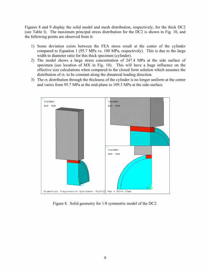
Figures 8 and 9 display the solid model and mesh distribution, respectively, for the thick DC2 (see Table I). The maximum principal stress distribution for the DC2 is shown in Fig. 10, and the following points are observed from it:

1) Some deviation exists between the FEA stress result at the center of the cylinder compared to Equation 1 (95.7 MPa vs. 100 MPa, respectively). This is due to the large width to diameter ratio for this thick specimen (cylinder).

2) The model shows a large stress concentration of 247.4 MPa at the side surface of specimen (see location of MX in Fig. 10). This will have a huge influence on the effective size calculations when compared to the closed form solution which assumes the distribution of σ1 to be constant along the dimateral loading direction.

3) The σ1 distribution through the thickness of the cylinder is no longer uniform at the center and varies from 95.7 MPa at the mid-plane to 109.3 MPa at the side-surface.

Figure 8. Solid geometry for 1/8 symmetric model of the DC2.

10

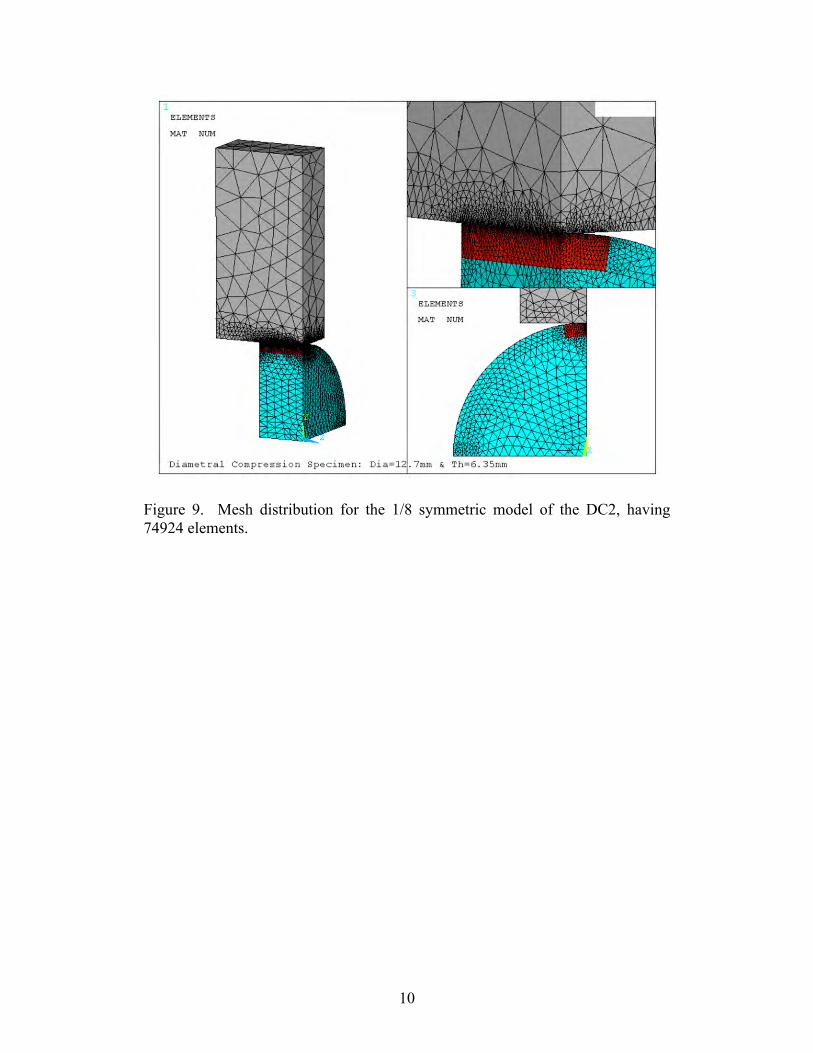
Figure 9. Mesh distribution for the 1/8 symmetric model of the DC2, having 74924 elements.

11

Figure 10. Maximum principal stress distribution (σ1) for DC2 of Fig. 8. Comparing the stress states for DC1 and DC2 suggests that the DC specimen approaches a plane strain condition instead of a plane stress condition as it gets wider (thicker). The derivation for the two dimensional stress state in the DC specimen is thoroughly outlined by Frocht in Ref. [6]. He utilizes the theory of elasticity to derive the stress equations. Using this approach, three fundamental principles must be satisfied: equilibrium, compatibility, and boundary conditions. It is through the compatibility equation that plane stress is distinguished from plane strain. However, when body forces (weights, inertial loading, etc.) are assumed to vanish, as is the case for this specimen, the compatibility equation for the plane stress condition becomes identical to that for the plane strain condition. Therefore, Frocht does not state whether the stress equations he derived for the DC specimen, including Equation 1 above which is referred to as the splitting strength equation in the ASTM standard, are for plane stress or plane strain condition. However, the fact that Frocht does not discuss the existence of σz (through thickness stress) indicates a plane stress condition. In addition he assumes the rectangular stresses (σx and σy) to be uniform across the thickness which is further indication a relatively thin disk is assumed. Figure 11 is obtained from Frocht’s book [Ref. 6] and displays the variation of σx and σy along the horizontal and vertical diametral directions. It is to be noted that σx and σy along the vertical and horizontal diametral axes are equal to the principal stresses σ1 and σ3 because of symmetry (shear stress = 0).

12

Figure 11. σx and σy distributions along the horizontal and vertical diametral directions (from [6]).

To further investigate the stress variation across the width for the DC1 (thin) and DC2 (thick) specimens, the maximum principal stress distributions at the mid-plane and side surface along the diametral loading axis were plotted in Figs. 12 and 13, respectively. Figure 12 shows the uniformity of the first principal stress (σ1) across the width for the thin cylinder as evidenced by the overlapping curves over the bulk of the vertical diametral axis of the specimen (away from the Hertzian stress region), while Fig. 13 indicates the opposite for the thick cylinder.

13

Figure 12. Comparison between maximum principal stress distributions at mid-plane and side surface along the loading axis for DC1. Radial location = 0 is at the center of disk.

Figure 13. Comparison between maximum principal stress distributions at mid-plane and side surface along the loading axis for DC2. Radial location = 0 is at the center of disk.

14

Timoshenko and Goodier [7] stated that plane stress condition exists in a thin plate loaded by forces applied at the boundary, parallel to the plane of the plate and distributed uniformly over the thickness. Under such conditions (similar to the DC1), the stress components σz, τxz, τyz are zero on both faces and within the plate. In addition, σx, σy and τxy do not vary across the thickness as was shown in Fig. 12 within the central region of DC1. Timoshenko and Goodier [7] defined plane strain to be the other extreme when the dimension of the body in z-direction (width) is very large. They stated if a long body is loaded with non-varying forces perpendicular to its longitudinal direction, then it may be assumed that all sections are in the same condition. The end sections can be thought of as if they were confined between fixed smooth rigid planes so that the displacement in the axial direction is prevented. Since εz = 0, then from Hooke’s law we can determine:

€

σ z = ν σ x + σ y( ) (2)

Figure 14 displays how σz varies across the central thickness for the thin DC1 and thick DC2 specimens. As can be seen, σz is zero throughout the thickness for DC1, further indicating that this specimen indeed satisfies plane stress condition. This is why the FEA and closed form stress solutions compare very well. On the other hand, for DC2 it can be seen that σz does not vanish throughout the thickness, and that it approaches zero only at the side face of the cylinder (normalized z/t =1). To compare the σz in the thick cylinder to the ideal plane strain condition, σz using Equation 2 was plotted as a function of thickness at the center of the specimen. The σx and σy substituted in this equation were obtained from the FEA results for DC2. Comparing the σz stress distributions for the DC2 specimen (red curve) with that expected in an ideal plane strain (green curve) indicates that this cylinder is somewhere between plane stress and plane strain conditions. This explains the small discrepancy between the FEA results and closed form solution as well as the stress variation across the thickness.

15

Figure 14. Comparison between σz stress distributions across central thickness of DC1 and DC2.

Figures 15 and 16 show the effective volume and effective area as function of Weibull modulus for the five DC specimens listed in Table I. The effective sizes were computed using the following equations:

−

=

−

=

fV

m

eV

Ve

fA

m

eA

Ae

PV

PA

11ln

11ln

0

0

σ

σ

σ

σ

, (3)

where Ae is the effective area, Ve is the effective volume, σ0 is the scale parameter, m is the Weibull modulus, σe is the maximum effective stress (computed using IDRS), and Pf is the probability of failure (also computed using IDRS). Of course the effective sizes are independent of the scale parameter since they only vary with stress distribution and the Weibull modulus. Hence, the scale parameter was assigned a random value in order to carry out the reliability and effective size calculations.

16

Figures 15 and 16 indicate that the effective sizes for the thick cylinders are smaller than that for the (thin) DC1 specimen. Additionally, these effective sizes are significantly smaller compared to the actual volumes and surface areas for the thick cylinders. This finding goes against intuition. The reason for this behavior is that when the effective size is computed, the stress distribution is normalized with respect to the maximum effective stresses in the component (σeA

and σeV in Equation 1). These stresses are computed using the IDRS using Gaussian points near the maximum stress location which in this case occurs below the top side surface of the specimens. This value is rather large for the thick cylinders (roughly 250 MPa), while relatively small for the thin cylinder (100 MPa). If this maximum effective stress is large (as is the case for the thick cylinders), then lower effective sizes are computed and vice versa.

Figure 15. Effective volume vs. Weibull modulus for the five DC specimens listed in Table I.

17

Figure 16. Effective area vs. Weibull modulus for the five DC specimens listed in Table I.

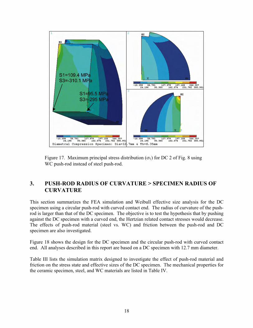
The effect of push-rod material on the stress state and effective sizes were also investigated. DC2 was reanalyzed using a WC push-rod instead of a steel push-rod. WC has an elastic modulus of 640 GPa and Poisson’s ratio of 0.24 (for a WC cermet containing 6% cobalt). Figure 17 shows the σ1 stress distribution in the bulk of the specimen excluding the Hertzian region. Comparing this to Fig. 10 (WC vs. steel push-rods) it can be seen that the stress states in the central region of the specimen are identical. In other words, the stress in the center of the DC specimen is unaffected by the push-rod material, as expected since this region is away from the contact zone between the push-rod and the DC specimen. However, the maximum stress at the side surface of the specimen increases as a result of using a stiffer material for the push-rod. This is expected to further decrease the effective sizes for the DC specimen, which is precisely what Figs. 15 and 16 show.

18

Figure 17. Maximum principal stress distribution (σ1) for DC 2 of Fig. 8 using WC push-rod instead of steel push-rod.

3. PUSH-ROD RADIUS OF CURVATURE > SPECIMEN RADIUS OF

CURVATURE This section summarizes the FEA simulation and Weibull effective size analysis for the DC specimen using a circular push-rod with curved contact end. The radius of curvature of the push-rod is larger than that of the DC specimen. The objective is to test the hypothesis that by pushing against the DC specimen with a curved end, the Hertzian related contact stresses would decrease. The effects of push-rod material (steel vs. WC) and friction between the push-rod and DC specimen are also investigated. Figure 18 shows the design for the DC specimen and the circular push-rod with curved contact end. All analyses described in this report are based on a DC specimen with 12.7 mm diameter. Table III lists the simulation matrix designed to investigate the effect of push-rod material and friction on the stress state and effective sizes of the DC specimen. The mechanical properties for the ceramic specimen, steel, and WC materials are listed in Table IV.

19

Table III. Simulation matrix for Section 3.

Push-rod material Push-rod geometry Friction state

Steel Curved contact end No friction Curved contact end No friction WC Curved contact end With high friction

WC Flat contact end With high friction

Table IV. Mechanical properties for the ceramic specimen, WC, and steel materials used in Section 3.

Property Ceramic WC Steel

Elastic Modulus (GPa) 450 640 200 Poisson’s ratio 0.17 0.24 0.3

20

Figure 18 shows a 1/8 symmetric solid model for the specimen. A circular push-rod with curved contact end is used to apply the load to the ceramic cylinder. The red sector seen in Fig. 18 under the push-rod was modeled where Hertzian related stress concentration would take place. Based on a parametric study to determine this region, the sector was given a depth of 1/10 the specimen’s radius and an angle of 16°. The volume and surface area corresponding to this red sector will not be included in the effective volume and area analyses because the high Hertzian stresses within this region would significantly skew the effective sizes for the DC specimen. In the FEA model, this red region was given a different material number than the ceramic material but still used the same mechanical properties as that for the ceramic. By doing so, the IDRS can discard this region from the effective size computations.

Figure 18. Solid geometry for 1/8 symmetric model of the DC specimen.

21

Figure 19 displays the mesh distribution used to simulate the DC specimen using 20-noded brick elements. Since the effective sizes are independent of the applied load magnitude in this specimen, an arbitrary load value (6334 N) computed using the closed form solution which induces a stress of 100 MPa at the center of the specimen was used for all simulations.

Figure 19. Mesh distribution for the 1/8 symmetric model of the DC specimen. The maximum principal stress distribution for the DC specimen with steel curved end contact push-rod and no friction is shown in Figure 20. The following can be observed from this figure:

1) FEA yields accurate stress results at the center of the cylinder compared to the closed form solution (99 MPa vs. 100 MPa, respectively).

2) Unlike the DC test using the flat rectangular push-rod that caused the maximum stress to occur at the side-surface (after ignoring the Hertzian region), in this case the maximum stress shifted to location MX as highlighted in Fig. 20.

3) The σ1 distribution through the central thickness of the disk varies slightly from 99 MPa at the mid-plane to 102.7 MPa at the side-surface. This could indicate slight deviation from plane stress state.

4) Similar to the flat push-rod test, the stress at the side-surface remains higher than that at the mid-plane when using the curved contact end push-rod.

22

Figure 20. Maximum principal stress distribution (σ1) for the DC specimen with steel curved end push-rod and no friction.

23

The maximum principal stress distribution for the DC specimen with WC curved end contact push-rod and no friction is shown in Figure 21. The following can be observed from this figure:

1) FEA yields accurate stress result at the center of the cylinder compared to closed form solution (98.8 MPa vs. 100 MPa, respectively).

2) Unlike the DC test with the steel curved end push-rod, the maximum stress shifted to the side surface of the specimen similar to the flat push-rod setup.

3) The σ1 distribution through the central thickness of the disk varies slightly from 98.8 MPa at the mid-plane to 102.5 MPa at the side-surface. This could indicate slight deviation from plane stress state.


Figure 21. Maximum principal stress distribution (σ1) for the DC specimen with WC curved end push-rod and no friction.

24

The maximum principal stress distribution for the DC specimen with WC curved end contact push-rod taking into account high friction (i.e., no slip) is shown in Figure 22. The following can be observed from this figure:

1) Friction has no influence on the stress state in the center of the specimen. However, it significantly reduces the maximum stress from 170 MPa to 129 MPa and shifts its location slightly down towards the center of the specimen. This will cause the effective size for the DC specimen taking into account friction to increase compared to that with no friction as will be shown below.

2) FEA yields accurate stress results at the center of the cylinder compared to closed form solution (98.3 MPa vs. 100 MPa, respectively).

3) Similar to the WC push-rod test with no friction, the maximum stress is located at the side surface of the specimen.

4) The σ1 distribution through the central thickness of the disk varies slightly from 98.3 MPa at the mid-plane to 101.9 MPa at the side-surface. This could indicate slight deviation from plane stress state.


Figure 22. Maximum principal stress distribution (σ1) for the DC specimen with curved end WC push-rod taking into account friction.

25

Figure 23 shows a 1/8 symmetric solid model for the specimen using a flat end push-rod. The maximum principal stress distribution for the DC specimen with the WC flat end push-rod taking into account high friction is shown in Figure 8. Comparing the stress distribution using curved end push-rod (Fig. 22) to that with flat end push-rod (Fig. 24), it can be seen that using flat end push-rod aggravates the situation by increasing the maximum stress at the side-surface from 129 to 179 MPa. This would in turn cause the effective size using the flat end push-rod to decrease.

Figure 23. Solid geometry for 1/8 symmetric model of the DC specimen with flat end push-rod.

26

Figure 24. Maximum principal stress distribution (σ1) for the DC specimen with flat end WC push-rod taking into account friction.

Figures 25 and 26 show the effective volume and effective area as function of Weibull modulus for the DC specimens listed in Table III. The curved end steel push-rod causes DC specimens to have the largest effective sizes. However, this analysis did not take into account friction and thus results are not expected to represent reality. Taking into account friction is expected to yield significantly lower effective sizes as was observed earlier. FEA analysis using steel push-rods with friction was attempted but the solution did not converge within reasonable time and hence was terminated. Figures 25 and 26 also indicate that by using a WC curved end instead of WC flat end push-rod and taking into account friction, the effective volume and area increase significantly. For example, using a Weibull modulus =10, the Ve and Ae using WC curved end rods increase by factors of 16 and 5, respectively, compared to tests using flat end push-rods. So it is obvious that using a curved end rod significantly improves the DC test results. However, this specimen remains inefficient in terms of the % of effective size to actual size ratio (see Fig. 27). For the specimen with a diameter of 12.7 mm and Weibull modulus of 10, the effective volume to volume ratio is approximately 0.8% while that for area is 1.7%.

27

Figure 25. Effective volume vs. Weibull modulus for the DC specimens listed in Table III.

Figure 26. Effective area vs. Weibull modulus for the DC specimens listed in Table III.

28

Figure 27. Area and volume efficiencies as function of Weibull modulus for the DC specimen using WC curved end push-rod and taking friction into account.

4. MATCHED RADII OF CURVATURE OF PUSH-ROD AND SPECIMEN This section summarizes the FEA simulation and Weibull effective size analyses using a push-rod whose radius of curvature matches that of the DC specimen. The effects of the WC push-rod arc-angle and friction on the effective sizes and maximum stress for the DC specimen are investigated. Figures 28 and 29 show 1/8 symmetric solid models for the DC specimen with 20° and 40° circular half-arc push-rods, respectively. All analyses described in this report are based on a DC specimen with 12.7 mm diameter, thickness to diameter ratio of t/d =1/4, and WC push-rod material. The red sector seen in Figures 28 and 29 under the push-rod were modeled where Hertzian stresses are high. Based on a parametric study to determine this region, the sector was given a depth of 1/10 the specimen’s radius and an angle 5° greater than that for the push-rod half arc-angle. The volume and surface area corresponding to this red sector will not be included in the effective volume and area analyses because the high Hertzian stresses within this region would significantly skew the effective sizes for the DC specimen. In the FEA model, this red region was given a different material number than the ceramic material but still used the same

29

mechanical properties as that for the ceramic. By doing so, the IDRS can discard this region from the effective size computations. Table V lists the simulation matrix constructed to investigate the effect of push-rod angular size and friction on the maximum tensile stress and effective sizes of the DC specimen. The mechanical properties for the ceramic specimen and WC materials are listed in Table VI.

Figure 28. Solid geometry for 1/8 symmetric model of the DC specimen with 20° circular half-arc push-rod. The red sector makes 25° half-arc.

30

Figure 29. Solid geometry for 1/8 symmetric model of the DC specimen with 40° circular half-arc push-rod. The red sector makes 45° half-arc.

Table V. Simulation matrix for Section 4.

Push-rod geometry Friction state 20° circular half-arc No friction 20° circular half-arc With high friction 40° circular half-arc No friction 40° circular half-arc With high friction

Table VI. Mechanical properties for the ceramic specimen, WC, and steel materials used in Section 4.

Property Ceramic WC Steel

Elastic Modulus (GPa) 450 640 200 Poisson’s ratio 0.17 0.24 0.3

31

Figure 30 displays the mesh distribution used to simulate the 20° half-arc DC specimen using 20-noded brick elements. Since the effective sizes are independent of the applied load magnitude in this specimen, an arbitrary load value (6334 N) computed using the closed form solution which induces a stress of 100 MPa at the center of a typical DC specimen was used for all simulations. The stresses developing at the center of the investigated specimens subjected to the proposed circular arc push-rods will then be compared to this 100 MPa value.

Figure 30. Mesh distribution for 1/8 symmetric model for the 20° half-arc DC specimen.

32

The maximum principal stress distribution for the DC specimen subjected to 20° half-arc WC push-rod and no friction is shown in Fig. 31. The following can be observed from this figure:

1) The maximum stress occurs at the center of the side-surface of the specimen. 2) The maximum stress is 88.6 MPa compared to 100 MPa in a typically loaded DC

specimen. 3) The σ1 distribution through the central thickness of the disk varies slightly. This could

indicate slight deviation from plane stress state.

Figure 31. Maximum principal stress distribution (σ1) for the DC specimen loaded with 20° circular half-arc WC push-rod and no friction.

33

The maximum principal stress distribution for the DC specimen subjected to 20° half-arc WC push-rod with friction is shown in Fig. 32. The following can be observed from this figure:


specimen. 3) Comparing Figs. 31 and 32, taking friction into account causes the maximum tensile

stress to decrease by about 12%. These two scenarios describe the two extremes of no friction and almost infinite friction.

4) The σ1 distribution through the central thickness of the disk varies. This could indicate slight deviation from plane stress state.

Figure 32. Maximum principal stress distribution (σ1) for the DC specimen loaded with 20° circular half-arc WC push-rod with friction.

34

The maximum principal stress distribution for the DC specimen subjected to 40° half-arc WC push-rod and no friction is shown in Fig. 33. The following can be observed from this figure:


specimen. 3) Compared to Fig. 31, as the angular size for the push-rod increases two things happen: a)

The stress decreases at the center of the specimen, and b) the region where tensile stresses develop gets smaller which would inevitably lead to smaller effective sizes.

4) The σ1 distribution through the central thickness of the disk varies slightly. This could indicate slight deviation from plane stress state.

Figure 33. Maximum principal stress distribution (σ1) for the DC specimen loaded with 40° circular half-arc WC push-rod and no friction.

35

The maximum principal stress distribution for the DC specimen subjected to 40° half-arc WC push-rod with friction is shown in Fig. 34. The following can be observed from this figure:

1) The maximum stress occurs near the center of the side-surface of the specimen. 2) The maximum stress is 37.9 MPa compared to 100 MPa in a typically loaded DC

specimen. 3) Comparing Figs. 32 and 34, taking friction into account causes the maximum tensile

stress to decrease by about 39%. These two scenarios describe the two extremes of no friction and almost infinite friction.

4) The σ1 distribution through the central thickness of the disk varies slightly. This could indicate slight deviation from plane stress state.

Figure 34. Maximum principal stress distribution (σ1) for the DC specimen loaded with 40° circular half-arc WC push-rod with friction.

36

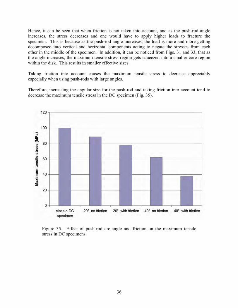
Hence, it can be seen that when friction is not taken into account, and as the push-rod angle increases, the stress decreases and one would have to apply higher loads to fracture the specimen. This is because as the push-rod angle increases, the load is more and more getting decomposed into vertical and horizontal components acting to negate the stresses from each other in the middle of the specimen. In addition, it can be noticed from Figs. 31 and 33, that as the angle increases, the maximum tensile stress region gets squeezed into a smaller core region within the disk. This results in smaller effective sizes. Taking friction into account causes the maximum tensile stress to decrease appreciably especially when using push-rods with large angles. Therefore, increasing the angular size for the push-rod and taking friction into account tend to decrease the maximum tensile stress in the DC specimen (Fig. 35).

Figure 35. Effect of push-rod arc-angle and friction on the maximum tensile stress in DC specimens.

37

Figures 36 and 37 show the effective volume and effective area as function of Weibull modulus for the DC specimens listed in Table V. As was discussed above, the matched radii design results in larger effective sizes. Hence, it is recommended for testing DC specimens. Of the two angles studied in Section 4, it is recommended that a push-rod with circular half arc-angle of 20° degrees be used to test DC specimens. This angle is not an optimized configuration, however. If this push-rod design is to be pursued further, then it is recommended that an optimization study be conducted to maximize the effective size of the DC specimen.

Figure 36. Effective volume vs. Weibull modulus for the DC specimens per Table V.

38

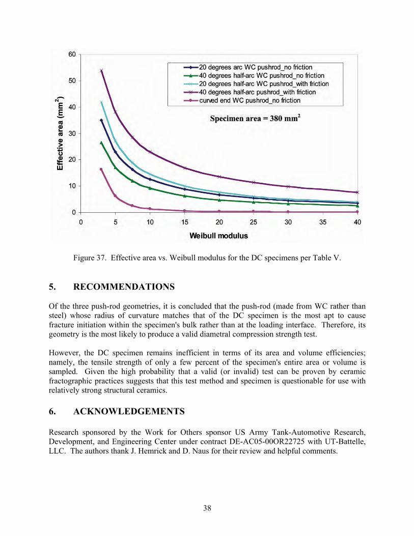
Figure 37. Effective area vs. Weibull modulus for the DC specimens per Table V. 5. RECOMMENDATIONS Of the three push-rod geometries, it is concluded that the push-rod (made from WC rather than steel) whose radius of curvature matches that of the DC specimen is the most apt to cause fracture initiation within the specimen's bulk rather than at the loading interface. Therefore, its geometry is the most likely to produce a valid diametral compression strength test. However, the DC specimen remains inefficient in terms of its area and volume efficiencies; namely, the tensile strength of only a few percent of the specimen's entire area or volume is sampled. Given the high probability that a valid (or invalid) test can be proven by ceramic fractographic practices suggests that this test method and specimen is questionable for use with relatively strong structural ceramics. 6. ACKNOWLEDGEMENTS Research sponsored by the Work for Others sponsor US Army Tank-Automotive Research, Development, and Engineering Center under contract DE-AC05-00OR22725 with UT-Battelle, LLC. The authors thank J. Hemrick and D. Naus for their review and helpful comments.

39

7. REFERENCES [1] F. L. L. B. Caneiro and A. Barcellos, "Concrete Tensile Strength," Union of Testing and

Research Laboratories for Materials and Structures, No. 13, March (1953). [2] T. Akazawa, "Tension Test Method for Concretes," Union of Testing and Research

Laboratories for Materials and Structures, No. 16, November (1953). [3] "Standard Test Method for Splitting Tensile Strength of Intact Rock Core Specimens,"

ASTM D3967, Vol. 04.08, ASTM International, West Conshohocken, PA, 2008. [4] M. Ferber, A. Wereszczak, and M Jenkins, “Fracture Strength,” Mechanical Testing

Methodology for Ceramic Design and Reliability, edited by D. Cranmer and D. Richerson, Marcel Dekker, 1998.

[5] A. Okada, “Diametral Compression Tests of Silicon Carbide Fibre-Reinforced Glass,” Journal of Materials Science, 25:3901-390 (1990).

[6] M. Frocht, Photoelasticity, Volume II, John Wiley & Sons, 1948. [7] Timoshenko and Goodier, Theory of Elasticity, McGraw-Hill, 1970.

ORNL-TM-2009/100 Effective Size Analysis of the Diametral ...

Documents

Transcript of ORNL-TM-2009/100 Effective Size Analysis of the Diametral ...