ork etw g N - nbcbn.net
115
Transcript of ork etw g N - nbcbn.net


GIS Based Decision Support Tool for Sustainable
Development of SUDD Marshes Region (SUDAN)
“Key knowledge”
By
Mohamed El Shamy
Eman Sayed
Mamdouh Anter
Ibrahim Babakir
Muna El Hag
Yasser Elwan
Coordinated by
Prof. Dr. Karima Attia
Nile Research Institute, Egypt
Scientific Advisor
Prof. Roland K. Price
UNESCO-IHE
Dr. Zoltan Vekerdy
ITC
2010

Produced by the
Nile Basin Capacity Building Network
(NBCBN-SEC) office
Disclaimer
The designations employed and presentation of material and findings through the publication don’t imply the expression of any opinion
whatsoever on the part of NBCBN concerning the legal status of any country, territory, city, or its authorities, or concerning the delimitation
of its frontiers or boundaries.
Copies of NBCBN publications can be requested from:
NBCBN-SEC Office
Hydraulics Research Institute
13621, Delta Barrages, Cairo, Egypt
Email: [email protected]
Website: www.nbcbn.com
Images on the cover page are property of the publisher
© NBCBN 2010

Project Title
Knowledge Networks for the Nile Basin
Using the innovative potential of Knowledge Networks and CoP’s in strengthening human
and institutional research capacity in the Nile region.
Implementing Leading Institute
UNESCO-IHE Institute for Water Education, Delft, The Netherlands (UNESCO-IHE)
Partner Institutes
Ten selected Universities and Ministries of Water Resources from Nile Basin Countries.
Project Secretariat Office
Hydraulics Research Institute – Cairo - Egypt
Beneficiaries
Water Sector Professionals and Institutions in the Nile Basin Countries
Short Description
The idea of establishing a Knowledge Network in the Nile region emerged after encouraging
experiences with the first Regional Training Centre on River Engineering in Cairo since
1996. In January 2002 more than 50 representatives from all ten Nile basin countries signed
the Cairo Declaration at the end of a kick-off workshop was held in Cairo. This declaration
in which the main principles of the network were laid down marked the official start of the
Nile Basin Capacity Building Network in River Engineering (NBCBN-RE) as an open
network of national and regional capacity building institutions and professional sector
organizations.
NBCBN is represented in the Nile basin countries through its nine nodes existing in Egypt,
Sudan, Ethiopia, Tanzania, Uganda, Kenya, Rwanda, Burundi and D. R. Congo. The
network includes six research clusters working on different research themes namely:
Hydropower, Environmental Aspects, GIS and Modelling, River Morphology, flood
Management, and River structures.
The remarkable contribution and impact of the network on both local and regional levels in
the basin countries created the opportunity for the network to continue its mission for a
second phase. The second phase was launched in Cairo in 2007 under the initiative of;
Knowledge Networks for the Nile Basin. New capacity building activities including
knowledge sharing and dissemination tools specialised training courses and new
collaborative research activities were initiated. The different new research modalities
adopted by the network in its second phase include; (i) regional cluster research, (ii)
integrated research, (iii) local action research and (iv) Multidisciplinary research.
By involving professionals, knowledge institutes and sector organisations from all Nile
Basin countries, the network succeeded to create a solid passage from potential conflict to
co-operation potential and confidence building between riparian states. More than 500 water
professionals representing different disciplines of the water sector and coming from various
governmental and private sector institutions selected to join NBCBN to enhance and build
their capacities in order to be linked to the available career opportunities. In the last ten
years the network succeeded to have both regional and international recognition, and to be
the most successful and sustainable capacity building provider in the Nile Basin.


CHAPTER 1. INTRODUCTION ..................................................................................................................... 1
1.1 DESCRIPTION AND LOCATION .................................................................................................... 1
1.2 PROBLEM STATEMENT ............................................................................................................... 1
1.3 STUDY OBJECTIVES .................................................................................................................... 2
1.4 SCOPE OF WORK ......................................................................................................................... 3
1.5 EXPECTED OUTPUTS .................................................................................................................. 3
1.6 USING THE RESULTS .................................................................................................................. 3
CHAPTER 2. REVIEW OF LITERATURE .............................................................................................. ....5
2.1 INTRODUCTION .......................................................................................................................... 5
2.2 SWAMP....................................................................................................................................... 5
2.2.1 Definitions ................................................................................................................................. 5
2.2.2 Types .......................................................................................................................................... 5
2.2.3 Examples of Swamps Areas ....................................................................................................... 6
2.3 MODELING OF SWAMPS ........................................................................................................... 11
2.3.1 Hydrological models ............................................................................................................... 11
2.3.2 Demand Forecasting Model .................................................................................................... 15
2.3.2.1 Demand Model Applications ................................................................................................... 15
2.4 WATER LOSSES ........................................................................................................................ 17
2.5 CLIMATE CHANGE ................................................................................................................... 20
2.5.1 Future Expectation .................................................................................................................. 20
2.5.2 Impact of climate change on water resources ......................................................................... 21
2.5.2.1 Hydrological cycle .................................................................................................................. 22
2.5.2.2 Precipitation............................................................................................................................. 22
2.5.2.3 Evapo-transpiration ................................................................................................................. 22
2.5.2.4 Soil moisture............................................................................................................................ 22
2.5.2.5 Ground water recharge ............................................................................................................ 23
2.5.2.6 River flow ................................................................................................................................ 23
2.5.2.7 Water quality ........................................................................................................................... 23
2.5.2.8 Lakes ....................................................................................................................................... 23
2.5.3 Sea level rise ............................................................................................................................ 24
2.6 RIVER NILE CLIMATE STUDIES ............................................................................................... 24
CHAPTER 3. SUDD NATURAL RESOURCES AND POTENTIAL ASSESSMENT ............................ 26
3.1 INTRODUCTION ........................................................................................................................ 26
3.2 ORIGIN AND DESCRIPTION ....................................................................................................... 26
3.3 THE SUDD AREA AND POPULATION ......................................................................................... 27
3.4 SUDD MARSHES NATURAL RESOURCES ................................................................................... 29
3.4.1 Vegetation ................................................................................................................................ 30
3.4.2 Distribution of Vegetation ....................................................................................................... 32
3.4.3 Topography ............................................................................................................................. 33
3.4.4 Climate .................................................................................................................................... 33
3.4.5 Wildlife and Mammals ............................................................................................................. 33
3.4.6 Birds ........................................................................................................................................ 33
3.4.7 Livestock production ............................................................................................................... 36
3.4.8 Fishing ..................................................................................................................................... 36
3.4.9 Tourism .................................................................................................................................... 37
3.4.10 Hunting .................................................................................................................................... 37
3.4.11 Oil production ......................................................................................................................... 37
3.5 DEVELOPMENT AND MANAGEMENT OPPORTUNITIES .............................................................. 37

3.6 DEVELOPMENT PRINCIPLES ..................................................................................................... 38
3.6.1 Ramsar Convention ................................................................................................................. 38
CHAPTER 4. SUDD BOUNDARY DELINEATION USING REMOTE SENSING ............................... 42
4.1 SOURCES OF SATELLITE IMAGES ............................................................................................. 42
4.2 DATA PROCESSING................................................................................................................... 44
4.2.1 Vegetation Index ..................................................................................................................... 44
4.2.2 Classification .......................................................................................................................... 45
4.2.3 Results and analysis ............................................................................................................... 46
4.3 SUDD BOUNDARY DELINEATION .............................................................................................. 47
4.3.1 Mapping the SUDD extent ..................................................................................................... 48
4.3.2 Methodology ........................................................................................................................... 48
4.3.3 Change Detection ................................................................................................................... 49
4.4 CONCLUSION ........................................................................................................................... 56
CHAPTER 5. SUDD HYDROLOGY AND CLIMATE .............................................................................. 58
5.1 INTRODUCTION ........................................................................................................................ 58
5.2 ANALYSIS OF HISTORICAL DATA ............................................................................................ 58
5.3 HYDROLOGICAL MODELING OF THE SUDD ............................................................................. 63
5.4 DISCUSSION AND CONCLUSION ............................................................................................... 72
CHAPTER 6. DEVELOPMENT INTERVENTIONS ............................................................................... 74
6.1 INTRODUCTION ...................................................................................................................... 74
6.2 DEVELOPMENT REQUIREMENT AND OPTIONS ...................................................................... 74
6.3 JONGLEI CANAL PROJECT ..................................................................................................... 74
6.3.1 Pre-Project Situation ............................................................................................................... 75
6.3.2 Project impact ......................................................................................................................... 78
CHAPTER 7. SUDD MARSHES MANAGEMENT TOOLS ..................................................................... 80
7.1 INTRODUCTION ...................................................................................................................... 80
7.2 MATHEMATICAL MODEL ...................................................................................................... 80
7.2.1 MIKE SHE model................................................................................................................... 80
7.3 MODFLOW MODEL .............................................................................................................. 81
7.4 DESIGN OF DECISION SUPPORT TOOL FOR SUSTAINABLE DEVELOPMENT OF SUDD AREA
……………………………………………………………………………………………….81
7.4.1 Background ............................................................................................................................ 81
7.4.2 Objectives ................................................................................................................................ 81
7.4.3 Brief Description of the System.............................................................................................. 82
7.4.3.1 Key Question to be addressed by the System ...................................................................... 82
7.4.3.2 Preconditions for System Development ............................................................................... 82
7.4.3.3 Selected information products to be generated (Indicators ) ............................................ 83
7.4.3.4 Setting Up the Baseline Model ............................................................................................. 83
7.4.3.5 Analyze the consequences ..................................................................................................... 83
Use Cases ............................................................................................................................................. 85
CHAPTER 8. REFERENCES ........................................................................................................................ 89
LIST OF RESEARCH GROUP MEMBERS

LIST OF FIGURE
Fig.1.1: Sudd marshes location in Sudan ...............................................................................................2
Fig.2.1: A forested swamp is dominated by trees with emergent vegetation. ......................................6
Fig.2.2: Skunk Cabbage (Symplocarpus foetidus) sprouts very early in the spring, melting the
surrounding snow. ..................................................................................................................................7
Fig.2.3: Examples of Cypress Swamps in USA ....................................................................................7
Fig.2.4:Examples of Okefenokee Swamp ..............................................................................................8
Fig.2.5: Location of the Sudd in southern Sudan.................................................................................10
Fig.2.6: Sudd Swamp from space, May 1993 (This photograph was taken during the driest
time of year—summer rains generally extend from July through September) ....................................11
Fig.2.7: Direct and indirect factors influencing water demand ...........................................................15
Fig.2.8: Outputs of the modeled water demand for the ACT .............................................................16
Fig.2.9: Projected Water Demand with Effects for Various Agriculture Water Usages .....................17
Fig.3.1: The Nuer tribes .......................................................................................................................28
Fig.3.2: Group of Children, Shilluk in Malakal and the Dinka tribes .................................................28
Fig.3.3: Sudd Marshes wetland ............................................................................................................30
Fig.3.4: Habitat for migratory birds in the Sudd marshes....................................................................35
Fig.3.5: Livestock resources in the Sudd Marshes ..............................................................................36
Fig.3.6: Finishing activity in Sudd area ...............................................................................................37
Fig.4.1: NDVI for the period 1-15 January 2003 .................................................................................42
Fig.4.2: Landsat 7ETM GeoCover mosaic ..........................................................................................43
Fig.4.3: Global Ecosystems .................................................................................................................43
Fig.4.4: Typical NDVI histogram distribution for LandSat image ......................................................44
Fig.4.5: Landsat tiles covered the Sudd area .......................................................................................45
Fig.4.6: Cross section infrared from Spot NDVI image, at the Sudd area ..........................................46
Fig.4.7: Classes for water and vegetations for different location at the study area .............................46
Fig.4.8: The boundary of Sudd Marshes .............................................................................................47
Fig.4.9: Sudd Digital Elevation Model ................................................................................................47
Fig.4.10: The Model Maker .................................................................................................................49
Fig.4.11: Monthly NDVI layer and cross section location ..................................................................49
Fig.4.12: NDVI values at cross section x-x .........................................................................................50
Fig.4.13: NDVI values along section y-y ............................................................................................50
Fig.4.14: NDVI values along section z-z .............................................................................................51
Fig.4.15: Trend of NDVI values along Sec X-X in different seasons ................................................53
Fig.4.16: Change in the green cover for Sudd during 1999-2006 .......................................................53
Fig.4.17: Comparison of change in green area during 1999-2006 ......................................................54
Fig.4.18: Spot NDVI for April, 1999 ...................................................................................................54
Fig.4.19: Spot NDVI for August, 1999................................................................................................55
Fig.4.20: Change in vegetation index between April and August for spot 1999 time series image ....55 Fig.4.21: The Maximum and Minimum buffers that surrounding the extents of the Sudd area .........57
Fig.5.1: Location Map of the Sudd region showing important flow gauges (triangles) and cities
(circles) - source: Elshamy (2006) .......................................................................................................58
Fig.5.2: Annual flow time series at the key stations in the Sudd region (1905-1982).........................59
Fig.5.3: Annual loss time series over the Sudd region (1905-1982) ...................................................60
Fig.5.4: Average monthly hydrographs at the key stations and of Losses over the Sudd region (1940-
1982) ....................................................................................................................................................60
Fig.5.5: Annual mean areal precipitation (MAP) for key sub-basins to the Sudd region....................61
Fig.5.6: Mean monthly areal precipitation (MAP) for the key sub-basins to Sudd region..................62
Fig.5.7: Water Balance Components of the Sudd ................................................................................62

Fig.5.8: Monthly Spatial Mean Rainfall and Evaporation Timeseries over the Sudd Swamp ............64
Fig.5.9: 10-day Water Levels of Juba and Mongalla on Bahr El-Jebel (1940-1983) ..........................65
Fig.5.10: Relationship between Mongalla and Juba levels ..................................................................66
Fig.5.11: Rating Curve of Mongalla (1970-1984 data) ......................................................................66
Fig.5.12: Juba levels and Estimated Mongalla levels (1997-2006) .....................................................67
Fig.5.13: Estimated vs. Measured Monthly Flows at Mongalla ..........................................................67
Fig.5.14: Performance of the HBV in Simulating the Flow of the Sobat@Hillet Doleib ..................69
Fig.5.15: Simulated Sobat Flows vs. Level Measurements (1998-2006) ............................................69
Fig.5.16: Flows at Mongalla, Hillet Doleib, and Malakal ...................................................................70
Fig.5.17: Estimated Monthly Sudd Losses ..........................................................................................70
Fig.5.18: Monthly Time series of Swamp Areal Extents.....................................................................71
Fig.5.19: Simulated vs. Observed Swamp Area ..................................................................................71
Fig.5.20: Modeled Swamp Area for 1940-1983 ..................................................................................72
Fig.6.1: The typical migratory cycle of livestock owners in the flood plain region ............................77
LIST OF TABLE
Table 2.1: Sudd mean losses in the highest and lowest months of the year. Mean discharge in
m3/sec. (source: Tottenham, 1913) ......................................................................................................18
Table 2.2: The budget of Jonglei Canal as an average discharge, year (1960). Mean monthly
discharge ( x 106 m3) and benefits. Source Jonglei Phase I, executive organ for the development
projects in Jonglei area, 1975...............................................................................................................19
Table 2.3: Summary of evaporation losses in Sudd Marshes area ......................................................19 Table 3.1: Population distribution in different section in Dinka and Nuer land traversed by the canal.
Source: Executive Organ for the Development Projects in Jonglei Area, 1979. .................................29
Table 3.1: Species resources in Sudd Marshes ...................................................................................33
Table 4.1: change in the green cover for Sudd area during 1999-2006 ...............................................51
Table 4.2: Output Classifications ........................................................................................................56
Table 6.1: Mean monthly timely discharges reaching Malakal ( x 106 m3) and the benefit realized
after regulation of Lake Albert and the Sudd diversion canal. ............................................................75
Table 7.1: proposed use cases for the SUDD area Decision Support System .....................................85

This report is one of the final outputs of the research activities under the second phase of the Nile Basin Capacity Building
Network (NBCBN). The network was established with a main objective to build and strengthen the capacities of the Nile basin
water professionals in the field of River Engineering. The first phase was officially launched in 2002. After this launch the
network has become one of the most active groupings in generating and disseminating water related knowledge within the Nile
region. At the moment it involves more than 500 water professionals who have teamed up in nine national networks (In-country
network nodes) under the theme of “Knowledge Networks for the Nile Basin”. The main platform for capacity building adopted
by NBCBN is “Collaborative Research” on both regional and local levels. The main aim of collaborative research is to strengthen
the individual research capabilities of water professionals through collaboration at cluster/group level on a well-defined
specialized research theme within the field of River and Hydraulic Engineering.
This research project was developed under the “Cluster Research Modality”. This research modality is activated through
implementation of research proposals and topics under the NBCBN research clusters: Hydropower Development, Environmental
Aspects of River Engineering, GIS and Modelling Applications in River Engineering, River Morphology, flood Management, and
River structures.
This report is considered a joint achievement through collaboration and sincere commitment of all the research teams involved
with participation of water professionals from all the Nile Basin countries, the Research Coordinators and the Scientific Advisors.
Consequently the NBCBN Network Secretariat and Management Team would like to thank all members who contributed to the
implementation of these research projects and the development of these valuable outputs.
Special thanks are due to UNESCO-IHE Project Team and NBCBN-Secretariat office staff for their contribution and effort done
in the follow up and development of the different research projects activities.


Resources are key factors in human survival and progress. Therefore, carful management and wise
use is needed to preserve human needs and ecosystem. Through the different phases of the Nile
Basin Capacity Building Network (NBCBN) for river Engineering scientists, engineers and specialist
have been working closely to conduct many research activities to protect and develop the available
water resources.
This report is an attempt to offer access to what has been done from research activity related to
Sudd Marshes region in southern Sudan.
The research team would like to express their appreciation to those who have made this
publication a reality, especially the management team of the NBCBN, and the research
technical advisors.


This research activity is one of research outputs conducted under the NBCBN. The main goal is to explore the
potential aspects to be developed in the Sudd Marshes region in southern Sudan. The Sudd is a vast swamp in
the lower of Bahr el Jebel (White Nile). Sudd was designated as a Ramsar site in 2006. The wise use of
wetlands according to Ramsar Convention is the sustainable utilization of the wetlands for the benefit of
mankind in a way compatible with the maintenance of the natural properties. The objectives are to improve
livelihood of the local people, reducing poverty, and conserving the ecosystem services. However, the
achievement of these objectives needs an accurate knowledge of the water balance components over the
wetland as well as the potential socioeconomic and environmental aspects. This research is an initiative
attempt to explore the potential entities can be used as a key knowledge for Sudd Marshes wetland
development.
From the available natural resources, it can be concluded that the ecology of the Sudd wetland is composed of
various ecosystems, grading from open water and submerged vegetation, to floating fringe vegetation,
seasonally inundated woodland, rain-fed and river-fed grasslands, and floodplain scrubland. It is a wintering
ground for birds of international and regional conservation importance such as Pelecanus onocrotalus,
Balearica pavonina, Ciconia ciconia and Chlidonias nigra; and is home to some endemic fish, birds,
mammalian and plant species, and to the vulnerable Mongalla gazelle, African elephant and shoebill stork.
Migratory mammals depend on the wetland for their dry season grazing. Hydrologically the Sudd wetland is
regarded as a giant filter that controls and normalizes water quality and a giant sponge that stabilizes water
flow. It is the major source of water for domestic, livestock, and wildlife use, and an important source of fish.
The occupants living within and adjacent to the Sudd region are almost exclusively Dinka, Nuer and Shilluk.
The socio-economic and cultural activities of these Nilotes are entirely dependent on the Sudd wetland and on
its annual floods and rains to regenerate floodplain grasses to feed their cattle. They move from their
permanent settlements on the highlands to dry season grazing in the intermediate lands (toich) at the
beginning of the dry season and return to the highlands in May-June when the rainy season starts. Oil
exploration as Sudd contains Sudan’s largest oil block has direct impact on the environment. There are
potential risks of air, water, and soil pollution for plants, wildlife, birds, livestock and human being. This may
result that the produced water contains toxic and cancerous chemical. Jonglei Canal Project, which is currently
on hold, but would reduce wet and dry season flows by 20 and 10% respectively, thus impacting the wetland’s
ecology and consequently its inhabitants. There are three protected areas within the Sudd, but no special
protection measures or management plan is in place. Therefore, the following potential can be defined for
management and developments:
Human livelihood
Land use management
Vegetation resource management
Livestock management (production and marketing)
Species management
Fisheries and aquacultures
Flood and draught threats management
Waste management
Wildlife management
Oil and water resource management
Hunting legalization
Tourism improvement and management
Water resource reservation
Settlement management
Impact of Jonglei Canal project on water resources and ecosystem

Due to the lack of field data, a methodology for mapping the Sudd extents using satellite images with
minimum field work was developed. The methodology is based on the vegetation index where the separation
of vegetation, open water, and soil can be possible. Different sets of images are used to achieve the study
objectives. Spot satellite NDVI product, Landsat satellite images, and SRTM digital elevation model are
among the used sets. Old topographic maps of the area are used as a ground truth dataset to verify the images.
The study results include maps of monthly average Sudd region extents, monthly surface area of open water
and vegetation, and land cover classification maps. The minimum and maximum buffers that surrounding the
extents of the Sudd area were estimated for both dry and wet seasons as 17,000 and 45,632 km2 respectively.
The study recommends that using additional sources of aqua-satellite images to define the actual extent of the
permanent and seasonal wetland to minimize the error from vegetation mixed with water.
Hydrological and hydraulic modeling of the Sudd are key to the understanding of the behavior of the wetland
and its role in shaping the ecology and the economy of the region. This has always been hindered by the
difficulty to monitor water levels and areal extents of this vast area from the ground. Satellite remote sensing
provides opportunities to avail information about the behavior of the wetland and this study attempts to utilize
such information to calibrate a hydrolological model of the wetland as an important component in building
knowledge about the area. The main objective of such model is to predict the swamp area and the Sudd
outflow to help evaluate the impacts of climate and land use changes over the area. The study used satellite-
based estimates of the Sudd area over the period 1999-2006 to calibrate a simple hydrological model of the
swamps. Other inputs to the model included rainfall over the swamps, evapotranspiration from swamp
vegetation, inflows estimated at Mongalla from levels measured at Juba, and outflows estimated as the
difference between White Nile flows at Malakal and Sobat flows at Hillet Doleib (estimated from a
hydrological model). Flow datasets were generally limited and had no overlap with the obtained series of areal
extents and thus records had to be completed using several methods. Rainfall over the Sudd area was found to
have a minor effect on the annual amount of losses. The inflow at Mongalla was found to be the most
controlling factor of the areal extents of, and therefore the losses from, the Sudd. Model performance was
inadequate due to several issues that had to be addressed. These include: calibration of satellite rainfall
estimates using available raingauges, ground truthing of estimated areas, and inclusion of inter-annual
variability of evapotranspiration (using global datasets or satellite-based algorithms like SEBAL and
METRIC), and probably revising model structure. A more complicated swamp model (including
hydrodynamic features) may be needed to improve the study results. However, data limitations have to be
overcome before increasing model complexity.
Sudd Marshes sustainable management required the compilation of local, national, and international
participations. In addition, the initiated and existing projects and programs should be taken into consideration
to identify priority areas of interventions. Some of these areas can be identified as follows:
1. Education.
2. Improving techniques.
3. Awareness and responsibility allocation among different stakeholders and various levels
4. Media engagement
5. Stakeholder analysis taken into consideration the distant stakeholders
6. Proper legislations for human and environments
7. Sustainable land use and land tenure systems
8. Water management for better management of soil and water conservation practices
9. Mechanism for mitigating disasters
10. Inventory and base map for available resources
11. Promote marketing of livestock at national and regional levels
12. Overgrazing management
13. Design livestock movement and raise awareness
14. Development of tools to influence policy makers
15. Conflict resolution mechanism through mitigation of over fishing and grazing
16. Define the tourism potential and capacity, Predict impacts, and apply safe environmental practices in
tourism activities

17. Policy safeguard for protected area
18. Avoid intervention and disturbance of migration routes
19. Impact assessment for any new project or exploration
20. Apply mitigation measures in suitable time
21. Establish quick technique to assess water pollutant
22. Establish an irrigation system for efficient management
23. Health facility for human and ecosystem
Key knowledge for management tools is introduced. Two mathematical models are defined; MIKESHE and
MODFLOW. The basic elements for designing Decision support system for the Sudd Marshes are also
highlighted.


ACT Australian Capital Territory
ANN Artificial Neural Network
CFCs ChlorFluoroCarbons
CGCM 3.1 The GCM model of the Canadian Centre for Climate Modeling & Analysis, Canada
CHARM Collaborative Historical African Rainfall Model
CNRM-CM3 The GCM model of the Meteo-France/Centre National de Researches
Meteorologique, France
CRU TS2.1 The time series data of the Climate Research Unit data, Version 2.1
CWPPRA Coastal Wetlands Planning, Protection and Restoration Act
ENSO El Nino Southern Oscillation
EPA Environmental Protection Agency
ETM+ Enhanced Thematic Mapper Plus
FAO Food and Agriculture Organization of the United Nations
GCMS General Circulation Models
GFDL Geophysical Fluid Dynamics Laboratory, USA
GIS Geographical Information System
GtC Gitatonnes of Carbon
HAD High Aswan Dam
HEC-HMS Hydrologic Modeling System (HMS) developed at the Hydrologic Engineering
Center (HEC) of the US Army Corps of Engineers
IMIS Integrated Management Information System
IPCC TAR Third Assessment Report of the Intergovernmental Panel on Climate Change
IPCC Intergovernmental Panel on Climate change
ITC International Institute for Goe-information Science and Earth Observation
MAP Mean Areal Preciptation
MWRI Ministry of Water Resources and Irrigation
NBCBN-RE Nile Basin Capacity Building Network for River Engineering
NDVI Normalized Difference Vegetation Index
NFC Nile Forecast Center
NFS Nile Forecast System
NGO Non Governmental Organization
NIR Near Infrared
NOAA-AVHRR National Oceanic Atmosphere Administration Advanced Very High Resolution
Radiometer
PET Potential Evapotransipiration
SDCWA San Diego Country Water Authority
SEBAL Surface Energy Balance Algorithm for Land
SISM Southern Illinios Swamp Model
SPLA Southern Sudanese Rebels
TAR Third Assessment Report
TM Thematic Mapper
UNESCO United Nation Educational, Science and Cultural Organization
USA United States of America
USGS United States Geological Survey
WAIS West Antarctic Ice Sheet


GIS and Modelling Research Cluster 2010
Nile Basin Capacity Building Network ( NBCBN ) 1
Chapter 1. Introduction
1.1 Description and location
The Sudd is a vast swamp (see Figure 1.1) located in Southern Sudan in the lower of Bahr el Jebel (White
Nile). The area which the swamp covers is one of the Africa’s largest tropical wetlands and the largest
freshwater wetland in the Nile basin. The Sudd stretches from Mongalla to just outside the Sobat
confluence with the White Nile just upstream of Malakal as well as westwards along the Bahr el
Ghazal. Its size is highly variable, averaging over 30,000 square kilometers. During the wet season it
may extend to over 130,000 km², depending on the inflowing waters, with the discharge from Lake
Victoria being the main control factor of flood levels and area inundation. A main hydrological
factor is that Sudd area, consisting of various meandering channels, lagoons, reed- and papyrus
fields, loses half of the inflowing water through evapo-transpiration in the permanent and seasonal
floodplains. The wetland supports a diversity of ecosystems with a rich flora and funa. The swamps consist
of wide blankets of high vegetation: papyrus, reeds, elephant grass, etc., which extend from the river bed to
the dry ground on either side, interrupted only by lagoons and side channels. To the west of the Sudd there are
the smaller wetlands of the central Baher el Ghazal Basin, and in the east is the Machar marshes of the Sobat
River. Sudd was designed as a Ramsar site in 5 June 2006, World Environment Day. In that day Sudan
announced the designation of the Sudd marshes as country’s second wetland of International Importance,
along with the Dinder National Park Ramsar Site and UNESCO Biosphere Reserve. However, the Sudd still
required an intensive assessment of its potential for wise use. The wise use of wetlands according to
Ramsar Convention is the sustainable utilization of the wetlands for the benefit of humankind in a
way compatible with the maintenance of the natural properties. The net objectives are to improve
livelihood of the local people, reducing poverty, and conserving the ecosystem services. However, Wetland
wise use and development requires an accurate knowledge of the water balance components over the wetland
as well as the potential socioeconomic and environmental aspects. This research is an initiative attempt to
explore the potential entities can be used as a key knowledge for Sudd marshes wetland development. This
research activity is supported by the Nile Basin Capacity Building network for River Engineering. The study
aims at introducing the key information and knowledge which can help in wise use of Sudd wetlands.
1.2 Problem statement
The Sudd is inhabited by the Nilotic tribes (Denka, Nuer, Shuluk), and is considered one of the harshest places
to live on earth. The area has been severely devastated by long civil wars. No doubt, the Sudd people are
amongst the poorest in the world, frequently hit by famines and starvation, caused primarily by social
instability, but possibly also by natural shocks such as drought and floods. However, the wetland is also well
endowed with rich natural resources to support the livelihoods of the people, while still maintaining the health
of the ecosystems. At present, the area is attracting large number of the displaced people after the peace
agreement of 2005. The Sudd Marshes is composed of permanent and seasonal swamps. The exact boundaries
of the swamp are difficult to specify. Attempts to define its size are based on hydrological models [Sutcliffe
and Parks, 1999], on remote sensing [Travaglia et al., 1995], or on both. The Sudd is generally very flat with
clayish soils. Rainfall is around 800 to 900 mm/yr, occurring from April to November. Daytime temperature is
on average 30-33°C during the dry season, dropping to an average of 26 to 28°C in the rainy season. The
relative humidity exceeds 80% during the rainy season, and drops to below 50% in the dry season. The
swamps and floodplains of the Sudd support a rich ecosystem, which is essential to the pastoral economy of
the local inhabitants. To the west of the Sudd there are the smaller wetlands of the central Baher el Ghazal
Basin, and in the east is the Machar marshes of the Sobat River.

GIS and Modelling Research Cluster 2010
Nile Basin Capacity Building Network ( NBCBN ) 2
Fig.1.1: Sudd marshes location in Sudan
The Jonglei Canal project aims at reducing the heavy water losses in the Sudd Marshes region which
are estimated to be about half of the river’s discharges passing Mongalla. This was to be achieved
through the construction of a diversion canal from Bor on Bahr El jebel to carry the water in excess
of Bahr el Jebel’s conveyance capacity without undue loss. Conservation of water and improvement
of the ecology of the Sudd region are the twin objectives of the Jonglei Canal project. The flood
regime and hydrology of Bahr el Jebel and the Sudd region in general limit any development in the
area. The provision of flood control, irrigation, drainage, and transportation facilities are a sine qua
non for unleashing the growth and development potential of this important region of the Sudan with
multiplier effects for the Sudanese economy at large. The canal aims at providing additional water
of about 5% of the Nile flow at Aswan, and it may dry 30% of the Sudd swamps [Howell et al.,
1988]. However, the work on the canal stopped in 1983 due to the civil war in Southern Sudan. The
signing of peace agreement between North and South Sudan is the starting point for developing the
southern part of Sudan. Developing and sharing natural resources is the biggest challenge for both
sides in particular water. This study will introduce the potential for integrated use of Sudd wetland
resources to improve livelihood of the local people, reducing poverty, and conserving the ecosystem
services. It will provide the tools and capacity for better decision making at the region taking into
consideration the possible effects of climate changes as well as the human intervention.
1.3 Study objectives
The study main objectives can be summarized as follows:
1. Detect the area changes (time series analysis) by using remote sensing data
2. Formulation of simple water balance model.
3. Calibration of the simple model to predict area, outflow based on remote sensing data.
4. Introducing the potential for sustainable development options of the Sudd area.

GIS and Modelling Research Cluster 2010
Nile Basin Capacity Building Network ( NBCBN ) 3
1.4 Scope of work
Literature review on the following topics:
1. Swamp definition and Types of wetlands and their ecological functions
2. Examples of swamps and their different functions
3. Hydrological modeling and water quality modeling of swamps
4. Losses in swamps
5. Climate Changes and their effects on water resources
6. Summary of previous studies on the Sudd region
Data collection on the Sudd region:
1. Images in different dates to represent High, medium, and low flood volume
2. Hydrological and meteorological parameters
3. Different resources in Sudd Area
4. Socioeconomic data (population, income, health, education, etc)
Time series analysis using remote sensing data
Water as a land cover class will be detected from the satellite image and verified using ground
truthing. The water detection will be applied using vegetation index technique and the ground
truthing will be obtained from supervised land cover classification of the satellite images.
Sudd Marshes Simulation tool (water balance model)
This tool will include simple hydrological (water balance) model, Sutcliffe and Parks (1987). The
model will be calibrated to predict area, and outflow based on remote sensing data. The tool frame
has to be developed using GIS technology.
Introducing the available resources and assessing the potential for developments
Developing different options for sustainable development of the area
Different development option and scenarios will be recommended.
1.5 Expected outputs
1. Geo-database
2. Strengthen the knowledge on the Sudd available resources
3. Hydrological model
4. Need assessment for future sustainable development
5. Sudd Marshes simulation tool
6. Ramsar related issues to be followed in the recommended development
1.6 Using the results
Many results (outputs) will be coming out of this research. The end user of the outputs are;
researchers, governmental institutions, Consultant, and NGO. The outputs will be disseminated by
different methods:

GIS and Modelling Research Cluster 2010
Nile Basin Capacity Building Network ( NBCBN ) 4
1. Sudd Marshes simulation tools and time series analysis
2. Deploy all the reports and literature review on the NBCBN web site.
3. Deploy the geo-database on the NBCBN site.
4. Publish the results in international conferences whenever it is possible.

GIS and Modelling Research Cluster 2010
Nile Basin Capacity Building Network ( NBCBN ) 5
Chapter 2. Review of Literature
2.1 Introduction
The Sudd marshes in Sudan is a very famous region and it attracts many of researchers and scientists
working in the field of water resources and hydrology. The sustainable development issues of
wetlands require multidisciplinary team and tremendous amount of literature to be reviewed. This
chapter represents a comprehensive literature review to highlight the state of the art in the fields of
swamp definitions, types, hydrological modeling, climate changes, and swamp sustainable
development.
2.2 Swamp
2.2.1 Definitions
A swamp is a wetland that features temporary or permanent inundation of large areas of land by
shallow bodies of water, generally with a substantial number of hummocks, or dry-land protrusions,
and covered by aquatic vegetation, or vegetation that tolerates periodical inundation. The water of a
swamp may be fresh water or salt water. A swamp is also generally defined as having no substantial
peat deposits.
Swamp could also be defined as forested wetlands. Like marshes, they are often found near rivers or
lakes and have mineral soil that drains very slowly. Unlike marshes, they have trees and bushes.
They may have water in them for the whole year or for only part of the year. Swamps vary in size
and type. Some swamps have soil that is nutrient rich; other swamps have nutrient poor soil. Swamps
are often classified by the types of trees that grow in them.
Swamps start out as lakes, ponds or other shallow bodies of water. Over time, trees and shrubs begin
to fill in the land. Plants die and decay and the level of the water gets lower and lower. Eventually,
the original body of water becomes a swamp.
2.2.2 Types
There are many different kinds of swamps, ranging from the forested red maple, (Acer rubrum),
swamps of the Northeast, to the extensive bottomland hardwood forests found along the sluggish
rivers of the Southeast. Swamps are characterized by saturated soils during the growing season, and
standing water during certain times of the year. The highly organic soils of swamps form a thick,
black, nutrient-rich environment for the growth of water-tolerant trees such as cypress (Taxodium
spp.), Atlantic white cedar (Chamaecyparis thyoides), and tupelo (Nyssa aquatica). Some swamps
are dominated by shrubs, such as buttonbush or smooth alder. Plants, birds, fish, and invertebrates
such as freshwater shrimp, crayfish, and clams require the habitats provided by swamps. Many rare
species, such as the endangered American crocodile depend on these ecosystems as well. Swamps
may be divided into two major classes, depending on the type of vegetation present: shrub swamps,
and forested swamps.
Forested swamps: are found throughout the United States (Figure 2.1). They are often inundated
with floodwater from nearby rivers and streams. Sometimes, they are covered by many feet of very
slowly moving or standing water. In very dry years they may represent the only shallow water for

GIS and Modelling Research Cluster 2010
Nile Basin Capacity Building Network ( NBCBN ) 6
miles and their presence is critical to the survival of wetland-dependent species like wood ducks (Aix
sponsa), river otters (Lutra iological), and cottonmouth snakes (Agkistrodon piscivorus). Some of the
common species of trees found in these wetlands are red maple and pin oak (Quercus palustris) in
the Northern United States, overcup oak (Quercus lyrata) and cypress in the South, and willows
(Salix spp.) and western hemlock (Tsuga sp.) in the Northwest. Bottomland hardwood swamp is a
name commonly given to forested swamps in the south central United States.
Fig.2.1: A forested swamp is dominated by trees with emergent vegetation.
Shrub swamps: are similar to forested swamps, except that shrubby vegetation such as buttonbush,
willow, dogwood (Cornus sp.), and swamp rose (Rosa palustris) predominates. In fact, forested and
shrub swamps are often found adjacent to one another. The soil is often water logged for much of the
year, and covered at times by as much as a few feet of water because this type of swamp is found
along slow moving streams and in floodplains. Mangrove swamps are a type of shrub swamp
dominated by mangroves that covers vast expanses of southern Florida.
2.2.3 Examples of Swamps Areas
United States: The most famous swamps in the United States are the Everglades, Okefenokee
Swamp and the Great Dismal Swamp. Swamps are often called bayous in the southeastern United
States, especially in the Gulf Coast region. In the USA, swamps are including a large amount of
woody vegetation. However, in Africa swamps are dominated by papyrus. By contrast a marsh in the
USA is a wetland without woody vegetation, or elsewhere, a wetland without woody vegetation
which is shallower and has less open water surface than a swamp. A mire (or quagmire) is a low-
lying wetland of deep, soft soil or mud that sinks underfoot.
Great Dismal Swamp: is located in northeastern North Carolina and southern Virginia. It is a
mixture of waterways, swamps and marshes (Figure 2.2). Unlike most swamps, it is not located near

GIS and Modelling Research Cluster 2010
Nile Basin Capacity Building Network ( NBCBN ) 7
a river. It is a coastal plain swamp. Trees like cypress, black gum, juniper, and water ash are
common. Animals commonly found in the Great Dismal Swamp include black bears, white-tailed
deer, opossum, raccoons, cottonmouth snakes.
Fig.2.2: Skunk Cabbage (Symplocarpus foetidus) sprouts very early in the spring, melting the surrounding
snow.
Cypress Swamps: are found in the southern United States (Figure 2.3). They are named for the bald
cypress tree. Bald cypress trees are deciduous trees with needle-like leaves. They have very wide
bases and ―knees" that grow from their roots and stick up out of the water. Bald cypress trees can
grow to 100 to 120 feet tall. Fire plays an important role in the establishment of bald cypress
swamps. Cypress trees grow very quickly after a fire and re-establish themselves before other trees
have a chance to grow! Many of the bald cypress trees in cypress swamps in the U.S. were cut down
in the late 1800s and the early 1900s. The wood from the bald cypress is resistant to rot and was a
popular wood for building. Other trees and shrubs like pond cypress, black gum, red maple, wax
myrtle, and buttonwood can also be found in cypress swamps. Animals like white-tailed deer, minks,
raccoons, anhingas, pileated woodpeckers, purple gallinules, egrets, herons, alligators, frogs, turtles
and snakes are often found in cypress swamps.
Fig.2.3: Examples of Cypress Swamps in USA

GIS and Modelling Research Cluster 2010
Nile Basin Capacity Building Network ( NBCBN ) 8
Okefenokee Swamp: Is located in southeastern Georgia and northern Florida (Figure 2.4). It is
about 25 miles wide and 40 miles long. Not all of the Okefenokee is a swamp part of it is a bog. In
fact, Okefenokee is an Indian word that means "Land of the Trembling Earth." Parts of the swamp
are so boggy that you can shake the trees by stomping on the ground. Trees in the Okefenokee
Swamp include giant tupelo and bald cypress. Mammals like the raccoon, black bear, white-tailed
deer, bobcats, red fox and river otter make the swamp their home. Reptiles in the swamp include the
eastern diamondback rattlesnake, cottonmouth, eastern coral snake, copper head, alligator and
snapping turtle. Birds like the barred owl, anhinga, great egret, great blue heron and sandhill crane
are also found in the swamp. Plants like the pitcher plant, water lily and iologi moss that grow in the
swamp can survive in the nutrient poor soil and acidic soil of the Okefenokee swamp.
Fig.2.4:Examples of Okefenokee Swamp
Asia- Asmat Swamp: is a wetland on the southern coast of New Guinea, located within what is now
the Indonesian province of Papua. It is sometimes claimed to be the largest alluvial swamp in the
world, it has an area of around 30,000 km². It is crossed by numerous rivers and streams, and large
areas are underwater at high tide. Ecologically, the swamp is diverse. The muddy coastal areas are
dominated by mangroves and nipah palms. Inland, where the swamp is fresh water, other sorts of
vegetation become more common, herbaceous vegetation, grasses, and forest. A significant portion
of the swamp is peat land. It is home to a wide variety of animals, including freshwater fish, crabs,
lobsters, shrimp, crocodiles, sea snakes, and pigeons. Also inhabiting the swamp are large monitor
lizards, some longer (although not as heavy) as the more famous Komodo Dragon. The swamp takes
its name from the Asmat people, who inhabit it. The difficult terrain of the swamp meant that the
Asmat did not have regular contact with outsiders until the 1950s, and the swamp still remains
isolated. The swamp forms part of Indonesia's Lorentz National Park.
The Vasyugan Swamp: (Russian: Васюганские болота) is one of the largest swamps in the world,
occupying 53,000 km² of western Siberia. The swamp is located in the Novosibirsk, Omsk, Tomsk
oblasts of Russia along the left bank of the Ob River. The swamp is a major reservoir of fresh water
for the region and several rivers find their sources there. The swamp is home to a number of
endangered species which is a concern among local environmentalists as the production of oil and
gas has become a major industry in the region.
South America- The Pantanal: is the world’s largest wetland area, a flat landscape, with gently
sloping and meandering rivers. The region, whose name derives from the Portuguese word ―pântano‖
(meaning ―swamp‖ or ―marsh‖ ), is situated in South America, mostly within the Brazilian states of
Mato Grosso and Mato Grosso do Sul. There are also small portions in Bolivia and Paraguay. In

GIS and Modelling Research Cluster 2010
Nile Basin Capacity Building Network ( NBCBN ) 9
total, the Pantanal covers about 150,000 square kilometers (58,000 sq mi). The Pantanal floods
during the wet season, submerging over 80% of the area, and nurturing the world's richest collection
of aquatic plants. It is thought to be the world’s most dense flora and fauna ecosystem. It is often
overshadowed by the Amazon Rainforest, partly because of its proximity, but is just as vital and
interesting a part of the neotropic.
The Paraná Delta: Is the delta of the Paraná River in Argentina. The Paraná flows north south and
becomes an alluvial basin (a floodplain) between the Argentine provinces of Entre Ríos and Santa
Fe, then emptying into the Río de la Plata. The Paraná Delta has an area of about 14,000 km² and
starts to form between the cities of Santa Fe and Rosario, where the river splits into several arms,
creating a network of islands and wetlands. Most of it is located in the jurisdiction of Entre Ríos, and
parts in the north of Buenos Aires.
Africa- Bangweulu: Is one of the world's great wetland systems, comprising Lake Bangweulu, the
Bangweulu Swamps and the Bangweulu Flats or floodplain. Situated in the upper Congo River basin
in Zambia, the Bangweulu system covers an almost completely flat area roughly the size of
Connecticut or East Anglia, at an elevation of 1140 m straddling Zambia's Luapula Province and
Northern Province. It is crucial to the economy and biodiversity of northern Zambia, and to the
birdlife of a much larger region, and faces environmental stress and conservation issues. With a long
axis of 75 km and a width of up to 40 km, Lake Bangweulu's permanent open water surface is about
3000 km², which expands when its swamps and floodplains are in flood at the end of the rainy season
in May. The combined area of the lake and wetlands reaches 15,000 km². The lake has an average
depth of only 4 m. The Bangweulu system is fed by about seventeen rivers of which the Chambeshi
(the source of the Congo River) is the largest, and is drained by the Luapula River.
The Okavango Delta (or Okavango Swamp): In Botswana, is the world's largest inland delta. The
area was once part of Lake Makgadikgadi, an ancient lake that dried up some 10,000 years ago.
Today, the Okavango River has no outlet to the sea. Instead, it empties onto the sands of the Kalahari
Desert, irrigating 15,000 km² of the desert. Each year some 11 cubic kilometers of water reach the
delta. Some of this water reaches further south to create Lake Ngami. The water entering the delta is
unusually pure, due to the lack of agriculture and industry along the Okavango River. It passes
through the sand aquifers of the numerous delta islands and evaporates/transpirates by leaving
enormous quantities of salt behind. These precipitation processes are so strong that the vegetation
disappears in the center of the islands and thick salt crusts are formed. The waters of the Okavango
Delta are subject to seasonal flooding, which begins about mid-summer in the north and six months
later in the south (May/June). The water from the delta is evaporated relatively rapidly by the high
temperatures, resulting in a cycle of cresting and dropping water in the south. Islands can disappear
completely during the peak flood, and then reappear at the end of the season.
The Sudd: Is a vast swamp formed by the White Nile in southern Sudan (Figure 2.5). Its size is
variable, but during the wet season it may be over 130,000 km² in area. In the Sudd, the river flows
through multiple tangled channels in a pattern that changes each year. Papyrus grows in dense
thickets in the shallow water, which is frequented by crocodiles and hippopotami. Sometimes the
matted vegetation breaks free of its moorings, building up into floating islands of vegetation up to 30
km in length. Such islands, in varying stages of decomposition, eventually break up. The sluggish
waters are host to a large population of mosquitoes and parasites that cause waterborne diseases. The
Sudd is considered to be nearly impassable either overland or by watercraft. The early explorers
searching for the source of the Nile experienced considerable difficulties, sometimes taking months
to get through. In the White Nile, Alan Moorehead says of the Sudd, "there is no more formidable
swamp in the world."

GIS and Modelling Research Cluster 2010
Nile Basin Capacity Building Network ( NBCBN ) 10
Fig.2.5: Location of the Sudd in southern Sudan.
There are three main waterways through the swamp; the Bahr al Zaraf ("River of the Giraffes"), Bahr
al Ghazal ("River of the Gazelles"), and the Bahr al Jabal ("River of the Mountain"), which is the
main connection to the Mountain Nile. Because of the Sudd swamp, the water from the southwestern
tributaries (the Bahr el Ghazal system) for all practical purposes does not reach the main river and is
lost through evaporation and transpiration (Figure 2.6). Hydrogeologists in the early part of the 20th
century proposed digging a canal east of the Sudd which would divert water from the Bahr al Jabal
above the Sudd to a point farther down the White Nile, bypassing the swamps and carrying the White
Nile's water's directly to the main channel of the river. The Jonglei canal scheme was first studied by
the government of Sudan in 1946 and plans were developed in 1954-59. Construction work on the
canal began in 1978 but the outbreak of political instability in Sudan has held up work for many
years. By 1984 when the Southern Sudanese rebels (SPLA) brought the works to a halt, 240km of
the canal of a total of 360km had been excavated. It is estimated that the Jonglei canal project would
produce 4.8 x 10⁹ m³ of water per year. There are, however, complex environmental and social
issues involved, which may limit the scope of the project in practical terms.

GIS and Modelling Research Cluster 2010
Nile Basin Capacity Building Network ( NBCBN ) 11
Fig.2.6: Sudd Swamp from space, May 1993 (This photograph was taken during the driest time of year—summer rains generally extend from July through September)
2.3 Modeling of swamps
2.3.1 Hydrological models
Doyle, 2009, conducted an ecological field and modeling study to examine the flood relations of
backswamp forests and park trails of the flood plain portion of Congaree National Park, S.C.
Continuous water level gages were distributed across the length and width of the flood plain portion
referred to as ―Congaree Swamp‖. To facilitate understanding of the lag and peak flood coupling
with stage of the Congaree River, a severe and prolonged drought at study start in 2001 extended into
late 2002 before backswamp zones circulated floodwaters. Water levels were monitored at 10 gaging
stations over a 4-year period from 2002 to 2006. Historical water level stage and discharge data from
the Congaree River were digitized from published sources and U.S. Geological Survey (USGS)
archives to obtain long-term daily averages for an upstream gage at Columbia, S.C., dating back to
1892. Elevation of ground surface was surveyed for all park trails, water level gages, and additional
circuits of roads and boundaries. Rectified elevation data were interpolated into a digital elevation
model of the park trail system. Regression models were applied to establish time lags and stage
relations between gages at Columbia, S.C., and gages in the upper, middle, and lower reaches of the
river and backswamp within the park. Flood relations among backswamp gages exhibited different
retention and recession behavior between flood plain reaches with greater hydroperiod in the lower
reach than those in the upper and middle reaches of the Congaree Swamp. A flood plain inundation
model was developed from gage relations to predict critical river stages and potential inundation of
hiking trails on a real-time basis and to forecast the 24-hour flood. In addition, tree-ring analysis was
used to evaluate the effects of flood events and flooding history on forest resources at Congaree

GIS and Modelling Research Cluster 2010
Nile Basin Capacity Building Network ( NBCBN ) 12
National Park. Tree cores were collected from populations of loblolly pine (Pinus taeda), baldcypress
(Taxodium distichum), water tupelo (Nyssa aquatica), green ash (Fraxinus pennslyvanica), laurel oak
(Quercus laurifolia), swamp chestnut oak (Quercus michauxii), and sycamore (Plantanus
occidentalis) within Congaree Swamp in highand low-elevation sites characteristic of shorter and
longer flood duration and related to upriver flood controls and dam operation. Ring counts and dating
indicated that all loblolly pine trees and nearly all baldcypress collections in this study are post
settlement recruits and old-growth cohorts, dating from 100 to 300 years in age. Most hardwood
species and trees cored for age analysis were less than 100 years old, demonstrating robust growth
and high site quality. Growth chronologies of loblolly pine and baldcypress exhibited positive and
negative inflections over the last century that corresponded with climate history and residual effects
of Hurricane Hugo in 1989. Stemwood production on average was less for trees and species on sites
with longer flood retention and hydroperiod affected more by groundwater seepage and site elevation
than river floods. Water level data provided evidence that stream regulation and operations of the
Saluda Dam (post-1934) have actually increased the average daily water stage in the Congaree River.
There was no difference in tree growth response by species or hydrogeomorphic setting to pre-dam
and post-dam flood conditions and river stage. Climate-growth analysis showed that long-term
growth variation is controlled more by spring/ summer temperatures in loblolly pine and by
spring/summer precipitation in baldcypress than flooding history.
Cynthia et al., 2002, developed a swamp hydrologic model to describe the spatial and temporal
distribution of the swamp hydrologic environment. The Okefenokee Swamp is a 160,000 ha
freshwater wetland in Southeast Georgia, USA, was divided into 5 sub-basins that reflect similar
seasonal hydrodynamics but also indicate local conditions unique to the basins. Topographic gradient
influences water-level dynamics in the western swamp (2 sub-basins), which is dominated by the
Suwannee River floodplain. The eastern swamp (3 sub-basins) is terraced, and the regional
hydrology is driven less by topographic gradient and more by precipitation and evapotranspiration
volumes. The relatively steep gradient, berm and lake features in the western swamp's Suwannee
River floodplain limit the spatial extent of the Suwannee River sill's effects, whereas system
sensitivities to evapotranspiration rates are more important drivers of hydrology in the eastern
swamp.
Xingchuan et al., 2002, presented a multi-scale model to simulate the impact of hydrologic changes
on the regeneration of a cypress swamp in southern Illinois. This model, SISM (Southern Illinois
Swamp Model), captures three processes that operate at different spatial and temporal scales: cypress
seed dispersal and germination, seedling growth and mortality, and the succession of saplings and
mature trees. In SISM, the life history of cypress is represented in a coherent manner, spatial-
temporal scales are related to different life phases, processes are consistently integrated, and the
interactions amongst the multiple processes are effectively simulated. Three scenarios reflecting
water management alternatives were tested and discussed. The results show that (1) the modeling
output under current water variability is comparable with various field studies, (2) a stable
hydrologic scenario restricts the spatial distribution of cypress, and (3) a more variable hydrologic
regime does not necessarily result in a wide regeneration of cypress.
In early 2001, the Coastal Wetlands Planning, Protection and Restoration Act (CWPPRA or Breaux
Act) Task Force approved a project that will return a minimum of 1,500 cubic feet/second(cfs)
Mississippi River flow to the Maurepas Swamp, restoring swamp hydrology, increasing sediment
and nutrient loading, and reinvigorating the Maurepas Swamp. Over 36,000 acres of wetlands will
benefit from this re-introduced river flow. The Environmental Protection Agency (EPA) was the lead
federal agency for the Maurepas project. Researchers at Louisiana State University completed
studies of hydrology (water movement), water quality, and ecology of the Maurepas Swamps. The

GIS and Modelling Research Cluster 2010
Nile Basin Capacity Building Network ( NBCBN ) 13
group developed a sophisticated computer model of hydrology to answer additional questions about
the possible effects of reintroduction of Mississippi River water into the swamps. This model
concluded that reintroducing Mississippi River water will reduce salt water intrusion into the
swamps, which can kill or weaken the cypress and tupelo trees. The model also reinforced earlier
predictions that nutrients in the river water would be almost completely taken up in the swamp
before the water reaches Lake Maurepas- in turn, supporting the earlier prediction that reintroduction
of Mississippi River water would not cause algal blooms in Lake Maurepas. The researchers also
developed a new computer ecological model of the swamp, called SWAMPSUSTAIN. The model
estimates the time it will take a reintroduction of Mississippi River water into the swamp to result in
target swamp elevations considered necessary for long-term sustainability of the swamp. The model
predicts that between 5,000 and 10,000 acres of the Maurepas swamp can be restored to
sustainability within 50 years if average yearly diversion discharges greater than 1,000 cfs are
maintained.
Schaake, J.C., et al., 1999, developed a hydrological swamp model for the two large swamps exist
in the basin, i.e. Bahr el Jebel and Machar (Sobat River Basin) swamps, which do not fit in the
concept of the gridded model that is being used in the rainfall-runoff hydrological modeling system
in the Nile Forecast Center (NFC), and are therefore modeled in the NFC by a swamp model. The
concept of the swamp model was developed by Sutcliffe, 1987. The model treats river and adjoining
swamps as separate reservoirs, with overflow from river to swamp. The models contain several
estimated parameters. They are swamp capacity and surface area, recharge, threshold level on
channel inflow for channel loss to occur, and maximum possible outflow from channel. It is essential
for better calibration of this model to have concurrent data on inflow, outflow and areal extent of
channel and swamp for different times in the year.
Mohamed et al., in 1999 conducted a regional climate model to the Nile Basin, with a special
modification to include routing of the Nile flood over the Sudd. The impact of the wetland on the
Nile hydroclimatology has been studied by comparing two model scenarios: the present climatology,
and a drained Sudd scenario. The results indicate that draining the entire Sudd has negligible impact
on the regional water cycle (atmospheric moisture fluxes, precipitation, evaporation, runoff and sub-
surface storage) and insignificant compared to the inter-annual variability of these parameters. In
terms of mass balance, the Sudd evaporated volume is a small fraction relative to the oceanic
moisture in the region (less than 1% of the atmospheric moisture in the Nile Basin). However, the
drained Sudd may create some climatic disturbances, which generate slightly higher rainfall than the
present situation. This is most likely attributed to an enhanced convective activity that occurs over
the dried wetlands. During the wet season the influence of the Sudd is not noticed. In the dry season,
when the Sudd may cause the largest impact on the water cycle, there is no mechanism for rainfall, at
least in major parts of the basin. The net gain of the Nile water by draining the entire Sudd wetland
would be an additional ~ 36 Gm3/yr (higher than observed Nile losses over the Sudd of 29 Gm3/yr).
This is about half the long-term mean of the Nile natural flow at Aswan. The famous Jonglei canal
phase I would drain about 30% of the Sudd wetland and save about 4 Gm3/yr (5% of the Nile flow at
Aswan). The runoff gain would then be up to ~ 36 Gm3 /yr. However, the impact on microclimate is
large. The relative humidity will drop by 30 to 40% during the dry season, and temperature will rise
by 4 to 6°C. The microclimate impact is confined to the Sudd area and the adjacent area to the west
and southwest direction influenced by the wind pattern in the dry season. During the wet season the
impact of the Sudd drainage is small, because the surrounding area is already saturated by the rain.
However, a slight decrease of relative humidity (<10%) is detected over the Sudd in the wet season.
Bauer, et al., developed a hydrological model for the Okavango Delta based on a finite difference
formulation of the relevant flow processes (surface and ground water) modeling software
MODFLOW (McDonald and Harbaugh, 1988). Spatially distributed input data include rainfall,

GIS and Modelling Research Cluster 2010
Nile Basin Capacity Building Network ( NBCBN ) 14
evapotranspiration and micropotography. The model results were compared to flooding patterns
derived from remote sensing. It has been shown that the flooding dynamics of the Okavango Delta
can in principle be understood and modeled in the framework of the two layer finite difference flow
model. Results showed that, once the model was calibrated and validated, it could be used to assess
the impacts of different management scenarios on the hydrological system. The model is particularly
useful to study long-term changes that result from different development scenarios.
Sutcliffe and Parks, 1987, developed a simple reservoir model for the swamps of the Sudd that is
responsible for the loss of much of the Nile outflow from Lake Victoria. At present only half of the
inflow of the Bahr el Jebel or White Nile at Mongalla emerges from the tail of the swamps. The
developed model used measured inflows and outflows and estimates of rainfall and evaporation to
reproduce volumes and areas of flooding over the historical period 1905-1980. Predicted outflows
based on inflows are then substituted for measured outflows so that the proposed diversions through
the Jonglei Canal can be incorporated in the model in order to predict the effects of the canal on
areas of flooding.
Georg Petersen, 2008, described the hydrology of the Sudd swamps in southern Sudan. The study
comprised a hydrologic investigation and evaluation of the Sudd water balance. The study improved
historical interpretations and unveiled so far unknown conditions and interdependencies in the
swamp and floodplain system, considering the area morphology, vegetation dynamics, water
balance, flow conditions and hydrodynamic processes in the system. The assessment was based on
field works carried out in the swamps over a three year period between 2004 and 2006 as well as
historical and remote sensing data. Interdependencies between morphology and hydrology were
described considering the effect of ground slopes and morphological features on spill and flooding of
the seasonally flooded grasslands. Bathymetric depth profiles and cross sectional depth and flow
distributions had been established for the Sudds inland delta and the question of spill into the Bahr el
Ghazal basin has been assessed. Vegetation dynamics in the swamp have been described and
quantified assessing the extent of changes in the channel and lagoon system of the Sudd using
Landsat satellite images for water body delineation. Changes in-between years and as well compared
to Lake Victoria outflow data have been established and quantified; correlation was found for the
largely water level dependent lagoon system. Variations in the channel system were interpreted to
happen in a certain pattern but the extent of changes could not be correlated to the outflow data as
they were influenced by additional, here not considered factors like wind drift and channel blockages
by vegetation. The water balances of the floodplains, while controlled by river levels, were found to
be dependent on a complex interaction between soil, vegetation, topography and seasonal trends in
rainfall and evapotranspiration. Based on field measurements, these components have been assessed
in detail and evaluated regarding their function in the seasonal cycle of flooding and drying. An
analysis of the soil and evapotranspiration conditions as well as the interaction with vegetation and
meteorological conditions using field and laboratory experiments was conducted. Sources, processes,
flow directions and the fate of the floodwaters on both the river fed seasonal floodplains and the
rainfed grasslands have been established showing that river spill was responsible for area flooding
while no return flow occured and drying was caused by evapotranspiration alone. Additionally it was
found that rainfall can only cause temporary flooding in extreme events. To obtain missing flow data
for important but ungauged locations, methods have been established to derive these, combining
upstream flows from Lake Albert and torrential runoff derived from the Collaborative Historical
African Rainfall Model (CHARM) rainfall data in the catchment between Lake Albert and Mongalla.
The results provided previously unavailable flow data at Mongalla, the entry to the Sudd swamp,
with a high level of confidence; data which were essential for detailed hydrological assessments of
the swamp system. In addition to evaluations based on measurements, a numerical hydrodynamic

GIS and Modelling Research Cluster 2010
Nile Basin Capacity Building Network ( NBCBN ) 15
assessment has been carried out with the DHI MIKE21 model. The study has established water level
gradients, flow directions and velocities in the swamp as well as on the seasonal floodplains.
2.3.2 Demand Forecasting Model
Water demand forecasting has become an essential component in effective water resources planning
and management. Water forecasts, together with an evaluation of existing supplies, provide valuable
triggers in determining when, or if, new sources of water must be developed. The importance of
accurate estimates of future water demands and their role in public planning is now well recognized.
Water demand models assume various forms. Models can be aggregated into simple and pliable
models or disaggregated by region, population, or location. Models also vary in the timeframe of the
data included and the breadth of the modeled processes. The demand forecasting model is
effectively incorporating changes in the social, economic, and environmental features when
predicting future water consumption in a growing region. Numerous factors can directly or indirectly
influence water demand. And these factors could be categorized as depicted in Figure 2.7.
Fig.2.7: Direct and indirect factors influencing water demand
2.3.2.1 Demand Model Applications
Australian Case: A water demand model has been developed for the ACT (Australian Capital
Territory) to predict the potential effects of future climate change. It is an aggregated model
combining daily water use data from ACTEW with a simple process based model that integrates user
behavior with different climate factors (maximum and minimum temperatures, solar radiation,
rainfall and vapor pressure). The model approach can separate out climate related demand from base
line demand not related to climatic factors. The model has been parameterized for the period 1995-
2000 (Figure 2.8) taking into account obvious changes in water use. Validation of the model was
carried out against data from earlier years, with results indicating a good fit. This approach provides
a significantly better description of water use than an approach using single climate factor alone,

GIS and Modelling Research Cluster 2010
Nile Basin Capacity Building Network ( NBCBN ) 16
such as evaporation. Historical climate files were adjusted to represent climate change scenarios and
user behavior adjusted to achieve the same level of utility from the water used. Changes in demand
were then expressed as proportions compared with base line usage. The measure of the water-use
efficiency for the ACT was based on non-climate driven water demand from 1965 to 2000. The drop
in water demand from around 1990 reflects behavioral changes in water use (in this case the switch
to grey water for public lands). The modeled versus simulated demand for the ACT for the period
1995 to 2000 was used to calibrate the model. Validation of the model was carried out by
determining the goodness of fit of the simulated data to the observed data from 1965 to 1994. The
open diamonds represent the calibrated period 1995-2000. A simple water demand model for the
ACT based on evaporation room the ―best case‖ to the ―worst case‖. In addition, mid-range values
were calculated from the CSIRO 2001 scenarios (1.25 C and 3 C for 2030 and 2070 respectively).
For 2030, the anticipated water demand increases from 1% to 5% with a mid-range value of 3%. By
2070 this range has increased to 1% to 16% with a mid-range value of 9%. The range of climate
change scenarios presented earlier in this report was used to assess likely changes per capita water
demand for the ACT for the years 2030 and 2070.
The full range of possible changes for each time period was assessed by combining the lowest
increase in temperature with the largest increase in rainfall and then the highest increase in
temperature with the greatest reduction in rainfall. Consequently the demand scenarios range These
proportional increases do not take into account the effects of changes in population or water-use
behavior. Population growth could be significant for the ACT with mid-range increases of 10% by
2030 and 14% by 2070. Higher range population scenarios are for increases of 30% by 2030 and
84% by 2070. The effect of these population changes are multiplicative with the per capita water
demand changes arising from climate change, leading to increased demand when combined. On the
other hand, there are a range of possible demand-management strategies which may limit increases
in water use. It would be possible using the approach described here to assess the effects of all three
factors combined as the method is based on per capita use and can alter user behavior.
Fig.2.8: Outputs of the modeled water demand for the ACT
The Egyptian case (WDFM Model): The Water Demand Forecasting Model was built within the
National Water Quality and Availability Management Project, Component 2000 which is
implemented in the MWRI, Planning Sector. There are two forms of the model; the first is a simple
form based on Spread (Excel) Sheet with proper links. The second is an Oracle-based Model using
the same components of water demand forecasting. The model operates as a standalone, or linked to
the Integrated Management Information System (IMIS) of the Planning Sector. In order to have
flexibility in developing the water forecasting models, the models are prepared as toolkits with input
variability of key model parameters. Effect analyses have been carried out to identify various impacts
on water demand forecasts caused by the underlying determinants of consumptions. These effects
are represented in the form of ranges of coefficients at the specific year of influence. The coefficients
are either positive indicating the relative increase in demand or negative showing a relative reduction
in demand. The values of these coefficients are gathered from the literature or past experience and
Per capita demand vs Evaporation
R2 = 0.74
0
200
400
600
800
1000
1200
1400
1600
1800
2000
0.00 2.00 4.00 6.00 8.00 10.00 12.00
mm/pan
L/p
ers
on
/yr
d c

GIS and Modelling Research Cluster 2010
Nile Basin Capacity Building Network ( NBCBN ) 17
then adjusted to the Egyptian circumstances. Figure 2.9 illustrates the total demand forecast up to
2020.
Tte San Diego Case: The San Diego Country Water Authority (SDCWA or the Authority), like
many major water resources agencies, faces a difficult task in forecasting water needs over a long
time horizon for a large service population. The water demand forecast typically forms the basis of
many decisions concerning the expected amount and timing of expenditures, such as additions to
supply and treatment capacity, implementation of water conservation programs, and changes to the
structure and level of water prices. Because water demand forecasts are often portrayed by a series of
point estimates, external parties can perceive them as if they are entirely accurate and certain.
Unfortunately, and by their very nature, such deterministic forecasts do not inform decision-makers
of the real uncertainties that are inherent to the forecasting process.
Fig.2.9: Projected Water Demand with Effects for Various Agriculture Water Usages
The presence and magnitude of these uncertainties can and should affect judgments concerning the
future. This study develops a probabilistic approach to water demand forecasting that offers the
opportunity to quantify and portray forecast uncertainty by improving and expanding upon the
Authority’s current water demand forecasting procedures to include statistical confidence intervals
around its extended long-term forecast (to 2030) of water demand. The SDCWA water forecasting
methodology for total demand consists of a system of econometric sector models, each adopting a
―rate of use times driver‖ approach to predict future demands. Sector models differ by their scope of
interest (whether single-family, multifamily, nonresidential, or agricultural), their accounting units or
driver variables (occupied living units, number of employees, or number of irrigated acres), and their
linear regression equations; however, they share common elements.
2.4 Water losses
Heavy losses of water occur in the Sudd region. On the average about half of Bahr El Jebel discharge
at Mongalla, before the river enters the swamps is lost when the river emerges from the swamps at
Malakal. Due to extensive growth of aquatic vegetable in the Sudd, the influence on evaporation
rates was studied to determine the role and contribution of the swamp vegetation to this heavy water
loss. Migahid (1948) conducted tank experiments to compare water loss from an open water surface
with that from a water surface covered with swamp vegetation. The proportion of water loss from the
Total Water Demand for Agriculture , Livestock, Fish Farming
for Egypt in Mm3/year
0
10000
20000
30000
40000
50000
60000
70000
80000
2001 2002 2003 2004 2005 2006 2007 2008 2009 2010 2011 2012 2013 2014 2015 2016 2017 2018 2019 2020
Years (2000-2020)
Wate
r D
em
an
d
Mm
3
Total Proj ected Water Demand For Various Agriculture Usages
Total Proj ected Water Demand For Various Agriculture Usages after Applying Effects

GIS and Modelling Research Cluster 2010
Nile Basin Capacity Building Network ( NBCBN ) 18
vegetation covered surface was also compared with that due to transpiration from the plant surface. It
was found that the water loss from a water surface covered with papyrus was about three times that
from an equivalent open-water surface but only one-third of the loss was attributed to physical
evaporation. Transpiration from the plant surface was found to cause two-thirds of the water loss.
Water loss due to evaporation was nearly equal, being 9.7 mm/day from open water and 9.8 mm/day
from vegetation-covered surfaces. In an earlier series of experiments the rate of evaporation during
the month of March for six successive years from 1926-32, was measured from a papyrus tank and a
Piche evaporimeter. Hurst (1952) found, from a series of the records, that the best measure of
evaporation rate from open water surface is to take the mean value of Piche evaporimeter from
several stations in a given area and then average them. In the literature there is no evidence to
indicate a special role of swamp vegetation in water loss from vegetation-covered surfaces as in the
case of the Sudd. Penman (1963), for example, maintains that ―transpiration from papyrus and
evaporation from the open lagoon are nearly equal‖ Rijks (1969) found that evaporation from a
papyrus swamp in Uganda was 60+ 15% of evaporation from an open water surface. The amount of
water lost in the swamps was determined from careful and extensive hydrological records of river
level and discharges upstream and downstream of the swamps (Tottenham, 1913). The study was
prompted by a report in 1904 (Garstin, 1904). The study of water losses, conducted over a period of
seven years 1905-06 to 1911-12, was directed to determine the percentage loss in the mean discharge
of Bahr el Jebel entering Mongalla, before it enters the swamp, and at Malkal after it has emerged
from the swamps. The percentage losses of Mongalla discharge was determined as the mean losses
per year, losses during June-November when the river is in flood, losses from December-May when
the rivers is falling, losses in the month of the highest and the month of the lowest discharge, and the
losses in the highest 10 day period of discharge and the lowest 10 days. These losses are given in
Tables 2.1 and 2.2.
Table 2.1: Sudd mean losses in the highest and lowest months of the year. Mean discharge in m3/sec. (source: Tottenham, 1913)
Mean discharge
Year Mongalla Malakal %loss Month
a) Highest month of the year
1906 1918 453 76 September
1907 1386 435 68 September
1908 1326 498 62 August
1909 1613 591 63 September
1910 1675 424 75 September
1911 967 384 60 September
1912 1175 431 63 September
Mean 1437.42 459.42 66.71
b) Lowest month of the year
1906 1027 512 50 March
1907 1016 507 50 March
1908 770 448 42 April
1909 756 464 38 March
1910 744 517 31 March
1911 649 439 24 March
1912 523 427 18 March
Mean 783.57 481.14 36.14

GIS and Modelling Research Cluster 2010
Nile Basin Capacity Building Network ( NBCBN ) 19
From the above data it can be concluded that around 500 m3/sec emerges at the tail with no concern
to the amount of water passing Mongalla. It is also concluded that the greater the volume of water
passing Mongalla the greater the percentage loss will be. As the discharge passing Mongalla
increases, so does the water level in the river channels. As the water reaches bankfull discharge it
cannot raise anymore, and consequently cannot travel any further to the northern end of the swamp.
Table 2.2: The budget of Jonglei Canal as an average discharge, year (1960). Mean monthly discharge ( x
106 m3) and benefits. Source Jonglei Phase I, executive organ for the development projects in Jonglei area, 1975.
JEBEL
Month Mongalla Jonglei
Canal
And Zeraf Total Daily
Gain
Monthly
Benefit
January 52.6 53.4 19.0 32.0 51.0 73.5 13.5 418.5
February 51.3 47.8 19.0 27.6 46.6 35.8 10.8 304.0
March 54.3 46.8 19.0 23.0 42.0 34.4 7.6 236.0
April 61.1 49.4 19.0 22.0 41.0 34.1 6.9 207.0
May 67.3 55.5 19.0 24.0 43.3 34.9 8.4 260.0
June 61.9 60.7 19.0 28.9 47.9 36.4 11.6 348.0
July 71.2 56.2 19.0 31.8 50.8 37.5 13.3 412.0
August 80.7 64.0 19.0 29.2 48.2 36.4 11.8 366.0
September 88.1 71.0 19.0 33.1 52.1 38.1 14.0 420.0
October 89.6 76.2 19.0 35.2 54.2 39.6 14.6 453.0
November 78.3 77.2 19.0 36.4 55.4 40.6 14.8 444.0
December 65.9 69.2 19.0 36.6 55.6 40.7 14.9 462.0
Mean Annual Benefit at Malkal = 4.33 x10⁹ m
3
Mean Annual Benefit at Malkal = 4.33 x10⁹ m
3 will be divided equally between Egypt and Sudan
who will share the cost of the project. Sudan’s share, measured at Malakal will be 2.35 x 10⁹ m
3. As
a result of the diversion, in an average year, downstream of the canal takeoff, the water levels of
Bahr el Jebel will be reduced by about 29 cm during the flood in September (average level 26.86 m)
and by 70 cm during the low season in March (average level 26.46 m). The levels of Bahr El Zeraf
will be reduced by 21 cm during the flood (average level 26.68 m) and by 40 cm during the low
season (average level 26.40 m). Table 2.2 is comparing the original (1936), the Equatorial Nile
canal (1948) and the present (1974) versions of Jonglei Canal. The comparison indicates the main
differences between the three status. A number of studies were conducted to estimate evaporation
losses from the Sudd area. The summary of these studies is illustrated in table 2.3.
Table 2.3: Summary of evaporation losses in Sudd Marshes area
Evaporation
(mm/yr)
Average
Sudd Area
(Gm2)
Source Method
1,533 7.2 Butcher, 1938 Measurement of Papyrus grown water
tank, aerial photo, water balance
8.3 Hurst and Black 1931 Water balance and limited surveys
2,400 Migahid, 1948 Lysimeter experiment on the Sudd
close to Bahr el Zeraf cuts
2,150 21.1 Sutcliffe and Parks,
1999
Water Balance
1,636 38 Mohamed, A. Y. 2005 Remote Sensing and SEBAl

GIS and Modelling Research Cluster 2010
Nile Basin Capacity Building Network ( NBCBN ) 20
2.5 Climate Change
Climate variations and change, caused by external forcing, come as a result of human activities, such
as the emission of greenhouse gases or land-use change. Therefore, one has to rely on carefully
constructed scenarios of human behavior and activities and determine climate projections on the
basis of such scenarios. However human activities are not considered the only part of the reality that
determines weather and climate. The growth, movement and decay of weather systems depend also
on the vertical structure of the atmosphere, the influence of the underlying land and sea and many
other factors not directly experienced by human beings. To understand the climate and its variations
we must understand the climate system, the system consisting of various components, including the
dynamics and composition of the atmosphere, the ocean, the ice and snow cover, the land surface
and its features, the many mutual interactions between them, and the large variety of physical,
chemical and biological processes taking place in and among these components. The climate system
is an interactive system consisting of five major components, the atmosphere, the hydrosphere, the
cryosphere, the land surface and the biosphere, forced or influenced by various external forcing
mechanisms, the most important of which is the Sun. Many physical, chemical and biological
interaction processes occur among the various components of the climate system on a wide range of
space and time scales, making the system extremely complex. Although the components of the
climate system are very different in their composition, physical and chemical properties, structure
and behavior, they are all linked by fluxes of mass, heat and momentum. Climate variations, is not
only result from radiative forcing, but also from internal interactions between components of the
climate system. A distinction can therefore be made between externally and internally induced
natural climate variability and change. Regional or local climate is generally much more variable
than climate on a global scale because regional or local variations in one region are compensated for
by opposite variations elsewhere.
Human activities, in particular those involving the combustion of fossil fuels for industrial or
domestic usage, and biomass burning, produce greenhouse gases and aerosols which affect the
composition of the atmosphere. The emission of chlorofluorocarbons (CFCs) and other chlorine and
bromine compounds has not only an impact on the radiative forcing, but has also led to the depletion
of the stratospheric ozone layer. Land-use change, due to urbanization and human forestry and
agricultural practices, affect the physical and 20iological properties of the Earth's surface. Such
effects change the radiative forcing and have a potential impact on regional and global climate to
which the climate system must act to restore the radiative balance. Heat is trapped in the atmosphere
through the greenhouse gases which consists of water vapor, carbon dioxide, methane and nitrous oxide. The
hydrological cycle continuously replenishes the world's water resources and is the foundation of life
on earth. Human activities are having disturbing influence on the cycle. Therefore understanding
short and long term climate change is the key element in defining the extreme climate events like
floods and draughts.
2.5.1 Future Expectation
The global annual emission of carbon dioxide from burning fossil fuel and other industrial processes
is estimated to have increased from about Gitatonnes of Carbon (GtC) in 1860 to almost 10 GtC by
the end of the 20th
century. Over the same period, the atmospheric concentration of Carbon dioxide
has increased from about 280 parts per million by volume (ppmv) to about 369 ppmv and the global
temperature of the earth has increased by about 0.6o C in the past 100 years, and is predicted to
continue to rise. Based on assessment of a number of future emissions scenarios of greenhouse gases

GIS and Modelling Research Cluster 2010
Nile Basin Capacity Building Network ( NBCBN ) 21
and aerosols, the intergovernmental Panel on climate change (IPCC) has projected that by the year
2100:
An average global warming of 0.7 to 2.5 o
C by 2050 with greater warming at higher latitudes
(IPCC 2001; Hennessy et al., 2002; Root et al., 2003). The globally averaged surface
temperature will warm by 1.4 to 5.8o C (relative to 1990)
Global mean sea level will rise by 9 to 88 cm (relative to 1990).
This projection is made up about half by thermal expansion of sea water, about one quarter
from melting of glaciers, and a small positive contribution from Greenland ice melt and
possibly a negative contribution from snow accumulation over Antarctica. However, the
contribution from Antarctica is especially uncertain, with recent events on the Antarctic
Peninsula raising the possibility of an earlier positive contribution from the West Antarctic
Ice Sheet (WAIS).
Precipitation will likely increase over the northern mid to high latitudes and Antarctica in
winter
Extreme events (drought, tropical, cyclone intensity) are likely to increase over some areas
There will be significant changes to snow cover and ice extent
A weakening of the large-scale-density-driven circulation in the ocean could be evident
These scenarios were regarded as plausible by the IPCC, but not assigned any probabilities. While
recent criticism of the technical basis of these scenarios is being considered by the IPCC, it is likely
that future projections will lie in roughly the same range, with values near the middle of the range
being more probable. Third Assessment Report of the Intergovernmental Panel on Climate Change (IPCC TAR) was
published in 2001. The TAR concluded that global warming has taken place over the last century,
and there is new and stronger evidence that most of the warming over the last 50 years is attributable
to human activities. It is likely that the 1990s was the warmest decade in the last 1000 years, at least
in the Northern Hemisphere. Other observations are consistent with this observed warming,
including a rise in global average sea level and ocean heat content, and decreases in snow cover and
ice extent both in mountain glaciers and Arctic sea ice. Recent evidence suggests that a predicted
slow-down in the deep ocean circulation driven by variations in temperature and salinity may also be
occurring. The TAR stated that it is likely there will be higher maximum temperatures and heat
indices over many land areas, and reduced frequency of low temperatures, including frosts. More
intense precipitation events are likely over many mid- to high-latitude land areas. Increased summer
continental drying and associated risk of drought are likely in mid-latitudes. Tropical cyclones are
projected to become more intense with higher peak winds and rainfall intensities. Other patterns of
climate variability, including the El Nino-Southern Oscillation (ENSO), may vary in intensity and
frequency, with some climate models suggesting more El Nino-like average conditions, and others
no change. Time lags in the ocean-atmosphere system mean that climate change, and especially sea
level rise, will continue long after stabilization of greenhouse gas concentrations in the atmosphere.
2.5.2 Impact of climate change on water resources
Water is inextricably linked with food security, human health and environmental protection. Rapid
population growth, increasing urbanization, industrialization and pollution threaten the sustainability
of our water resources. Natural climate variability and human induced climate change add to those
threats, particularly in developing countries where the impacts are potentially great and the capacity
to cope is weakest. The following subsections are highlights of some impacts on water resources.

GIS and Modelling Research Cluster 2010
Nile Basin Capacity Building Network ( NBCBN ) 22
2.5.2.1 Hydrological cycle
A significant proportion of the solar energy received by the earth is used in driving the hydrological
cycle. Greater greenhouse gas concentrations in the atmosphere mean an increase of the available
energy on the surface of the earth and thus according to the basics of thermodynamics, an
"intensification" of the hydrological cycle. At the global scale, all climate model simulations have
verified this (Kabat et al., 2003). The expected intensification of the hydrological cycle will not be
experienced merely as a smooth linear trend, but rather in the form of oscillations (for example
ENSO). The oscillations may be more frequent than in the past and the amplitude of the variability
may also increase over some areas. The climate changes alter the route and residence time of water
in the watershed and change its quality. As a result water might be unsuitable as a resource.
2.5.2.2 Precipitation
The IPCC third assessment report (IPCC TAR) summarizes projected precipitation trends as a
general increase in mean annual precipitation in the Northern Hemisphere (Autumn and winter) and
a decrease in the tropics and sub-tropics in both hemispheres. The frequency of extreme rainfall is
likely to increase with global warming, although the spatial resolution of global climate models is too
coarse to provide details. Higher temperatures imply that a smaller proportion of precipitation may
fall as snow.
Precipitation changes are more spatially variable than projected temperature changes. Although a
general increase in precipitation is expected, some regions will see large increases, while others will
see significant reductions. There is still quite a bit of uncertainty about the prediction of
precipitation, for two main reasons:
Precipitation is a secondary process in General Circulation Models (GCMs) and as such, is
poorly represented
Heavy precipitation systems frequently occur on scales that are considerably smaller than the
typical grid scale of GCMs, which is two to three degrees of latitude/longitude.
2.5.2.3 Evapo-transpiration
Increased temperatures result in an increase in potential evaporation. In dry regions, potential
evaporation is driven by energy and is not constrained by atpospheric moisture contents. In humid
regions, however, atmospheric moisture content is a major limitation to evaporation. Studies show
increases in evaporation with increased temperatures. Vegetation also plays an important role in
evaporation, partially by intercepting precipitation and partially by determining the rate of
transpiration. Higher CO2 concentrations may lead to increased water use efficiency i.e. water use
per unit of biomass, implying a reduction in transpiration. However, higher CO2 concentrations may
also be associated with increased plant growth, compensating for increased water use efficiency.
Plants may thus acclimatize of evaporation is constrained by water availability.
2.5.2.4 Soil moisture
Runs with the HadCM2GCM show that increases in greenhouse gases are associated with reduced
soil moisture in the Northern Hemisphere summers. This is the result of higher winter and spring
evaporation, caused by higher temperatures and reduced snow cover, and lower rainfall during the

GIS and Modelling Research Cluster 2010
Nile Basin Capacity Building Network ( NBCBN ) 23
summer. The lower the water holding capacity of the soil, the greater is the sensitivity to climate
change.
2.5.2.5 Ground water recharge
Increased winter rainfall may result in increased groundwater recharge in the Northern Hemisphere.
However, increased temperatures may increase the rate of evaporation, which leads to longer periods
of soil water deficits. Shallow unconfined aquifers along floodplains in semiarid regions are
recharged by seasonal stream flows and can be depleted directly by evaporation. Changes of the
duration of flow in those streams may lead to reduced groundwater recharge. Sea level rise could
cause saline intrusion to coastal aquifers, especially in shallow aquifers. An overlying bed that is
impermeable, on the other hand, characteristics a confined aquifer and local rainfall does not
influence the aquifer.
2.5.2.6 River flow
Most hydrological studies on the effect of climate change have concentrated on stream flow and
runoff. Stream flow is water flowing in a river channel, whereas runoff is defined as the amount of
precipitation that does not evaporate. Although there are many hydrological models simulate river
flows using climate scenarios derived from GCMs, relatively few studies have been published for
Africa, Latin America and South East Asia. Responses in different hydroclimates may be quite
different. The following four examples illustrate this:
Cold and cool temperate climates: Stream flows in these areas are largely dependent on
melting snow in spring time. The most important effect of climate change is the timing of
stream flow. There will be more runoff during winter because less precipitation falls as snow.
Mild temperate climates: These regions are dominated by rainfall and evaporation. The
magnitude of the flows is determined largely by rainfall changes. Trends show a decrease in
summer runoff and an increase in winter runoff.
Semi arid and arid regions: Here a small percentage of change in rainfall causes considerable
effects in runoff
Tropical regions: runoff responses are largely dependent on rainfall. The number of extreme
events causing flooding may increase due to increased in precipitation.
2.5.2.7 Water quality
Agricultural practices may change as a result of climate change. Agriculture chemical loads in
surface and groundwater may therefore change accordingly. Furthermore, higher temperatures may
decrease the concentration of Oxygen and thus increase eutrophication.
2.5.2.8 Lakes
Closed (endorheic) lakes with no outflow are especially vulnerable to changes in climate conditions.
These lakes are considered as good indicators of the effects of climate change. Exorheic lakes may
also be sensitive to climate change. For example, levels of lake Victoria in East Africa have
increased for several years following increases in precipitation levels.
Observational evidence indicates that climate changes in the 20th
century have already affected a
diverse set of physical and biological systems. Examples of observed changes with linkages to

GIS and Modelling Research Cluster 2010
Nile Basin Capacity Building Network ( NBCBN ) 24
climate include shrinkage of glaciers; thawing of permafrost; shifts in ice freeze and break-up dates
on rivers and lakes; increases in rainfall and rainfall intensity in most mid- and high latitudes of the
Northern Hemisphere; lengthening of growing seasons; and earlier flowering dates of trees,
emergence of insects and egg-laying in birds. Statistically significant associations between changes
in regional climate and observed changes in physical and biological systems have been documented
in freshwater, terrestrial and marine environments on all continents except Australia (see Hughes,
2003).
2.5.3 Sea level rise
Melting ice and thermal expansion of the oceans are the two primary drivers of sea level rise. As the
sea rises, there are four main impacts that are:
Increased coastal erosion: Sea level rise, more extreme weather, and a loss of sea ice will
contribute to more erosion and flooding along vulnerable Arctic shorelines. Higher sea levels
with less ice cover will expose more of the coast to both normal waves and more powerful
storm waves.
Flooding, inundation and displacement of wetlands and lowland: land presently at the
margins of tide and wave action may be inundated and accelerated erosion of dunes may
occur in response to higher wave action associated with raised water levels.
Impairment of water quality in freshwater aquifers and estuaries: due to low elevation and
small hydraulic gradient, coastal plain groundwater resources of the southeastern United
States are potentially vulnerable to salinisation from sea level increase. Saline intrusion in the
lower reaches of the deltas would be aggravated by the predicted sea level rise and may
warrant revised management of flow control
Reduced protection from extreme storm and flood events: higher sea levels provide a higher
base for storm surges to build on, making severe floods more likely.
2.6 River Nile Climate Studies
Siam, 2010, studied the impact of climate change on the upper Blue Nile catchments flows using the
IPCC scenarios. The Upper Blue Nile catchment supplies Egypt with nearly 60% of its annual
transboundary share. Meteorological data from three different sources (CRU, University of
Delaware and Rain gauges from MWRI) are analyzed and the most accurate is selected for
downscaling. Three statistical downscaling techniques (Delta, ANN, Bias-Correction) are
investigated for three chosen GCMs (The Canadian CGCM 3.1, the French CNRM-CM3 and the
American GFDL-CM2); each tested for the two IPCC scenarios; the mid-high (A2) and the low
scenarios (B1). The results of downscaling are used as inputs for the hydrological modeling to
predict the upper Blue Nile catchment flows while testing two different approaches; artificial neural
network (ANN) and HEC-HMS. The corresponding range of change in flow values is transferred to
the High Aswan Dam (HAD) as historically correlated with flows arriving at Roseiras dam (While
assuming that patterns for climate change for the Equatorial plateau are similar to those for the
Ethiopian plateau) in order to estimate the future change in the Nile flows arriving at Aswan for the
remainder of the current century. The results showed a possible decrease by about 20% under the
GFDL model and a probable increase by about 40% under the CNRM model both using the A2
scenario.

GIS and Modelling Research Cluster 2010
Nile Basin Capacity Building Network ( NBCBN ) 25
El.Shamy et al., (2009) used the output of 17 GCMs with the SRES A1B emission scenario to
investigate the impacts of climate change on the Upper Blue Nile catchment flows for the period
from 2081 to 2098. The temperature and the precipitation are downscaled using the bias-correction
approach. The baseline has been selected to be 1961–1990 as this is the period for which most
climate centers have submitted daily data for the 20th century climate experiment (20c3m). The
observed rainfall dataset has been obtained from the NFS (Nile Forecast System) as gridded daily
rainfall for the period 1992-2006. However, these two periods don't overlap; the effect of this
difference on the long-term mean water balance has been found to be small as there is little
difference in the mean monthly rainfall distribution for the two periods. Changes in total annual
precipitation range from −15% to +14% and temperature from 2oC to 5oC and consequently PET to
increase by 2-14%. The NFS hydrological model hosted by the MWRI is used to get the
corresponding flow of each scenario. The results show that the ensemble mean annual flow at Diem
is reduced by 15% compared to the baseline. However, the very high sensitivity of flow to rainfall
makes such a number highly uncertain. There is some evidence that higher reductions in rainfall may
be accompanied by higher increases in PET possibly due to reductions in cloud cover. This further
enhances the effect of rainfall reduction on runoff leading to very high reductions in the mean annual
flow for some models (up to 60%). Some models predicted large increases as well (up to 45%).
A more detailed modeling effort was undertaken by Yates and Strzepek (1998) in a climate change
assessment for the Nile basin. Lumped hydrologic models and lake/swamp models for the entire Nile
system were developed and calibrated on a monthly basis. Six different GCM experiments were used
in the assessment. GCM temperature and precipitation changes were interpolated to a 0.5° x 0.5° grid
for use with the hydrologic models. GCM projections of Lake Victoria temperature changes ranged
from 2 to 2.7° C with precipitation changes between -0.2 to +26%. Blue Nile changes ranged from
2.2 to 3.7°C and -8.8 to +55% for temperature and precipitation, respectively. Modeled Blue Nile
flows ranged from -32 to +133%, while Lake Victoria 22 flows ranged from -35 to +104%. The
study concluded that river flows were especially susceptible to precipitation changes (Tidwell, 2006).
Conway and Hulme (1996) used three climate scenarios in a study of the sensitivity of Nile river
flows to potential climate change. One dry and one wet scenario were selected from GCM
experiments, and a third scenario was constructed from a weighted average of seven models. The
Composite precipitation scenario was generated from a weighted mean of seven equilibrium GCM
change fields (Hulme, 1994). Each GCM was given a weighting based on its ability to simulate
current precipitation. The temperature changes were given equal weights in the composite scenario.
For measuring the corresponding flows, a hydrological model for the Blue Nile catchment is divided
into 10-minute latitude by 10-minute longitude grid cells. Estimates of mean monthly precipitation
and evapotranspiration are calculated for all grid cells and fed into a simple monthly water balance.
The runoff obtained for each cell is then summed to produce an overall estimate of catchment runoff.
The model has three adjustable parameters that are assumed constant for all grid cells except for the
cells representing the Lake Tana and Dabus swamp subcatchments. The grid cells in these two
subcatchments require different parameter values in order to simulate the storage and delaying effect
on runoff from these hydrologically special areas. For Lake Victoria an existing monthly water
balance model of the lake catchment was used. Simulated changes in runoff ranged from -8.7 to
+15.3% for the Blue Nile and from -9.2% to +11.8% for Lake Victoria, with just one scenario
predicting decreases in the two basins. While Lake Victoria demonstrated greater sensitivity to
temperature changes than the Blue Nile, the study found that both were more susceptible to changes
in precipitation than temperature.

GIS and Modelling Research Cluster 2010
Nile Basin Capacity Building Network ( NBCBN ) 26
Strzepek and Yales (1996) developed a one dimensional water balance model to investigate the
possible impacts of climate change over the whole Nile basin. Three GCMs and hypothetical
scenarios based on sensitivity analyses are used. To assess climate change effects, the GCM grids
were overlaid on the historic monthly temperature and precipitation surfaces in the GIS. The change
in temperature between the l x and 2x CO2 scenarios for each grid cell was considered constant over
the cell and was added to the historic value to produce a new temperature surface for that month. The
precipitation change (as a ratio of climate change to base values) was overlaid on the historic
precipitation surface and then multiplied to produce a new precipitation surface. Catchments'
weighted-average climate parameters were calculated from the new temperature and precipitation
surfaces. For the sensitivity analyses, spatially homogeneous changes in temperature (+2 and +4oC)
and precipitation (±20%) were applied to the reference climate parameters. Two of the GCMs show a
decrease in the flow at Aswan by 22% and 77%, the third model shows an increase by 30% relative
to the average of the historic values from 1900 to 1972.
Chapter 3. Sudd Natural Resources And Potential Assessment
3.1 Introduction
Sudd marshes have scientific, socioeconomic and political value by the fact that they have a major
role in the conservation of biodiversity. The swamps and floodplains of the Sudd support a rich
ecosystem, which is essential to the pastoral economy of the local inhabitants. However, the
prospective for potential development is still not clearly identified due to the significant knowledge
gaps. This chapter introduces the data collection related to different aspects. The main objectives are
to develop a GIS based simulation tool for sustainable development of the Sudd marshes. The
intended development will be created through development intervention to improve the living
conditions of all people in and around the Sudd area, to create alternative livelihoods, to alleviate
poverty, to enhance agriculture productivity, and to protect and preserve the biodiversity and
environments.
3.2 Origin and description
Sudd word was originally used to refer to the blockage by vegetation as an obstruction to river
navigation. It has also become a synonym for permanent swamps. The Sudd area lies between
coordinates 6o 30′ – 9 o
30′ N and 30 o
10′ – 31 o 45′E. It is considered as the largest tropical wetland
in the world with an elevation of 350 – 450 m asl. The Sudd area is approximately 5,700 000 ha
(246,111 km2). The Sudd region has, been classified into four land categories according to flood
liability of each type. These categories are: High land, intermediate land, toich and Sudd or
permanent swamps.
The High Land: The ground elevations are standing no more than a few centimeters above the
general terrain. They are scattered ridges in the terrain. They have permeable soil and, because of
their elevation, have better drainage. These high lands provide the only refuge for man and animals
during the high rainy season where extensive flooding occurs elsewhere.
The Intermediate Land: This is the extensive and flat clay plain lying to the east of Bahr El Zeraf.
As the name indicates, the topography of this land is intermediate between that of the high grounds
and the toich or water meadows adjacent to river banks. The landscape is a typical expanse of open
grassland. During the rainy season they are subject to flooding or at least severe water logging.

GIS and Modelling Research Cluster 2010
Nile Basin Capacity Building Network ( NBCBN ) 27
During the dry season they are waterless. Sometimes, and as a result of the combination of heavy
rainfall and the flatness of the land waves of flood advance across the clay plain. This is referred to
as the ―creeping flow‖.
The Toich: Toich is a local word meaning land seasonally flooded by water spills from rivers (or
other water courses) and where the soil retains sufficient moisture during the dry season to support
the growth of pasture. They vary in area and type of pasture grass depending on the hydrological
conditions of the sustaining river or water channel.
Sudd: This land formation consisting of permanent swamps for the greater part of the year occurs
immediately below the toich level. The soils have a thick layer of peat covering mineral soil of
alluvial origin.
3.3 The Sudd area and population
It found in three locations as follows:
A narrow southern belt 10 km wide and 146 km long (Mongalla to Bor). This area is
inhabited by the Mundari and the Dinka tribes
The flat central portion of gradient 1.0-1.5 cm/km. This portion extends from Bor to lake No
with the largest width of 40 km and a depth of at least 10 m. This part is inhabited by both
the Dinka and the Nuer tribes.
A narrower northern portion extending from Lake No to the confluence of Bahr el Zeraf
within the White Nile of 2 km wide. This portion is inhabited by the Nuer Shilluk and the
Dinka tribes.
The Sudd area is prone to seasonal annual flooding (July- December) and highly evaporation volume
of water from the extended swamps. As mentioned above the Sudd area is inhabited by three main
group or tribes: the Shilluk, Nuer and Dinka. The last two groups include various inter-tribal sections
within each tribe. The land of the Shilluk is around and the north of the outfall of the Jonglei canal.
The Nuer (Figure 3.1) lives to the south of River Sobat and east Bahr El Zeraf. The southern Dinka
country extends north from south of the canal takeoff at Bor to the southern limit of the Nuer
country. Both the Nuer and Dinka countries will be traversed by the Jonglei canal. The northern
Dinka lives between the Shilluk in the north and the Nuer to the south. The Shilluk land will be only
indirectly affected by the canal.
The Shilluk live (Figure 3.2) in villages built on the higher land along the alluvial banks of the White
Nile. They changed relatively recently from a predominantly migratory to a more or less sedentary
life. They still own livestock but their economy has been extended to crop production and fishing in
addition to limited animal production. On the average they own less cattle than the Dinka or Nuer
and their livestock consists mainly of sheep. Their livestock husbandry is less elaborate. No cattle
camps are normally established as distances between dry season toich grazing and the permanent
village are short.
The Nuer people are primarily pastoralists and the preoccupation with cattle is the most important
feature of their life (Evans-Pritchard, 1940). They on the high lands in homesteads widely separated
from each other. Although a limited amount of crop production is practiced, cattle represent a
reliable alternative or insurance against crop failure. Fishing represents another economic activity
particularly at the beginning and end of the rainy season.

GIS and Modelling Research Cluster 2010
Nile Basin Capacity Building Network ( NBCBN ) 28
Fig.3.1: The Nuer tribes
The Dinka, like the Nuer, are also primarily pastoralists, but limited crop production and fishing are
subsidiary economic activities. It is stated by Deng (1973) that the Dinka are over occupied by their
cattle to an extent which limits optimal utilization of the resources of their land. The southern Dinka,
south of the Nuer land, lives in villages on high lands more closely settled than those of the Nuer but
not as compact as the villages of the Shilluk.
Fig.3.2: Group of Children, Shilluk in Malakal and the Dinka tribes
There are no detailed data on human demography in the area. Recent estimates of the total
population living in the area traversed by the Jonglei canal give a total of 260, 740 people, belonging
to the Dinka and Nuer groups. The estimate does not include the third group, the Shilluk, since they
live strictly outside the Jonglei area and their land is not traversed by the canal. The population
density distribution (Table 3.1) in the area increase from north to south with the highest density in
the southern Dinka land in Kongor and Bor district.
Despite the variation in human population density between the Dinka and Nuer people whose land
will be traversed by the Canal, their mode of life and pattern of land use are very similar and
ecologically determined. They migrate with their cattle in rhythmic seasonal movements, the extent
of which is determined by the land availability.

GIS and Modelling Research Cluster 2010
Nile Basin Capacity Building Network ( NBCBN ) 29
Table 3.1: Population distribution in different section in Dinka and Nuer land traversed by the canal. Source: Executive Organ for the Development Projects in Jonglei Area, 1979.
Subsection
Section Area (km2) Total population Density per km
2
A 539
3,870
974
4.870
1.002
20113
34.234
8.279
32.045
6.593
37.50
11.43
8.50
6.58
6.58
B 1.135 42.5563 37.29
C 483
227
564
52.563
8.513
1.664
109.29
37.50
2.90
D 483
403
52.787
1.168
109.29
2.89
Total 14.550 260.746 17.32
Distribution of High Lands, Intermediate Lands, toich grazing and water, except during the rainy
season when both human and animal population settle in the permanent villages on the High Lands
away from the flooded plains, life for the rest of the year is managed from cattle camps sited in the
Intermediate Lands or the toiches at various distances from the villages. This annual transhumant
migration of people and livestock represents an example of adaptation to the local environment and
rational utilization of the grazing resources in the area. The cycle of migration starts from the
permanent villages in about November, when the dry season has commenced, with a movement
westwards towards the intermediate lands. It ends in May or June, when the river water and the rainy
season sets in, with a return movement eastwards to the high lands. The rate of movement in both
direction is gradual but is influenced by the availability of grazing and water when moving west
towards the river, or by early rising flooding in the toich hastening an early eastwards movement
through the intermediate land back to the permanent village sites on the high land.
The Shilluk, unlike the Nuer or the Dinka have the Intermediate and Toich grazing in the vicinity of
their villages, and as a consequence have been able to attend more to cultivation of crops. They
cultivate four types of land. Around the homesteads cowpea, gourd, marrow, water melon, tobacco
and maize are grown in late May or as soon as sufficient rain has fallen. Quick maturing red-grained
sorghum is also planted at about the same time interplant with sesame, and when harvested in August
the stalks are allowed to ratoon shifting cultivation is practiced in the intermediate land where a
white-grained sorghum, tolerant of flooding, is grown. In the dry season small vegetable plots are
established along the alluvial banks of the White Nile, often with irrigation.
3.4 Sudd Marshes natural resources
Ecologically the Sudd wetland (Figure 3.3) encompasses a number of different ecosystems, grading
from open water and submerged vegetation, to floating fringe vegetation, seasonally inundated
woodland, rain-fed and river-fed grasslands, and floodplain scrubland.
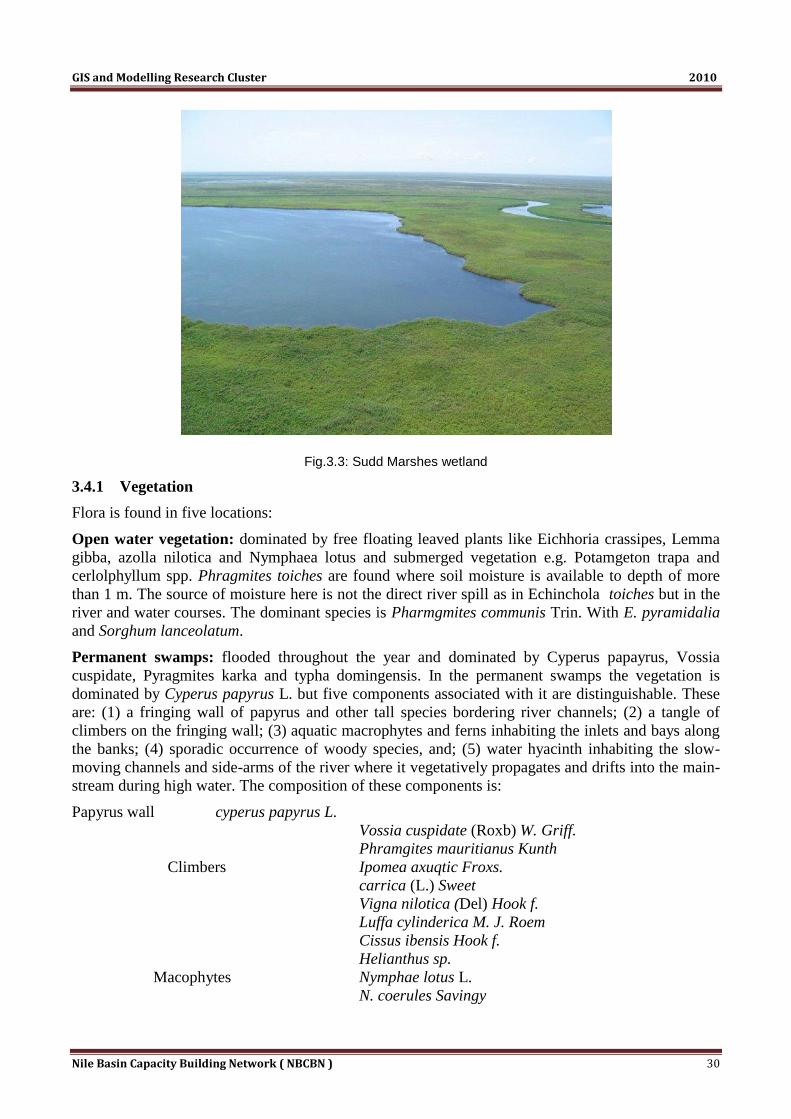
GIS and Modelling Research Cluster 2010
Nile Basin Capacity Building Network ( NBCBN ) 30
Fig.3.3: Sudd Marshes wetland
3.4.1 Vegetation
Flora is found in five locations:
Open water vegetation: dominated by free floating leaved plants like Eichhoria crassipes, Lemma
gibba, azolla nilotica and Nymphaea lotus and submerged vegetation e.g. Potamgeton trapa and
cerlolphyllum spp. Phragmites toiches are found where soil moisture is available to depth of more
than 1 m. The source of moisture here is not the direct river spill as in Echinchola toiches but in the
river and water courses. The dominant species is Pharmgmites communis Trin. With E. pyramidalia
and Sorghum lanceolatum.
Permanent swamps: flooded throughout the year and dominated by Cyperus papayrus, Vossia
cuspidate, Pyragmites karka and typha domingensis. In the permanent swamps the vegetation is
dominated by Cyperus papyrus L. but five components associated with it are distinguishable. These
are: (1) a fringing wall of papyrus and other tall species bordering river channels; (2) a tangle of
climbers on the fringing wall; (3) aquatic macrophytes and ferns inhabiting the inlets and bays along
the banks; (4) sporadic occurrence of woody species, and; (5) water hyacinth inhabiting the slow-
moving channels and side-arms of the river where it vegetatively propagates and drifts into the main-
stream during high water. The composition of these components is:
Papyrus wall cyperus papyrus L.
Vossia cuspidate (Roxb) W. Griff.
Phramgites mauritianus Kunth
Climbers Ipomea axuqtic Froxs.
carrica (L.) Sweet
Vigna nilotica (Del) Hook f.
Luffa cylinderica M. J. Roem
Cissus ibensis Hook f.
Helianthus sp.
Macophytes Nymphae lotus L.
N. coerules Savingy

GIS and Modelling Research Cluster 2010
Nile Basin Capacity Building Network ( NBCBN ) 31
Najas pectinata (Parl.) Magnus
Ottelia ulvifolia (Planch) Walp
Vallisneria aethiopica fenzl
Ultricularia thonningii Schumach
Pistia stratoites L.
Polygonum sp.
Ceratophyllum demersum L.
Trapa bipinosa Roxb
T. natans
Ferns Dryopteris gongyloides
Azolla niltica
Dryopteris gongyloides
Azola nilotica
Woody plants Aeschynomomene elphroxylon
(Guillem, and Perrot.) Taub
Allien plants Eichhornia crassipes (Mart.) Solms
River flooded grassland: dominated by Pyragmites, Sorghum, Hyperhenia and Selaria grasses as
well as Oryza and Echinchloa. This is a most productive grassland type for livestock and wild life
grazing. Where flooding persists for longer periods as a result of rise in water levels when coupled
with the peak of the rains, Echinochloa toiches flourish. Here the dominant grass species are E.
stagnina (Retz) Beauv. And E. Pyramidalis (Lam). Hitch. & Chase with Oryza barthii(A. Chev.),
O.punctata and Vossia cuspidate (Roxb.) W. Griff. As associates. E. stagnina and V. cuspidate
generally occur where flooding is longer and deeper and where the soil remains moist during the dry
season. E. pyramidalis and Oryza species are limited to areas where the depth and duration of
flooding is less. Echinochloa toiches are the only source of reliable green grazing available to
livestock during the dry season. The northwestern edge of the region in the swamps of Bahr el
Ghazal is characterized by slightly different types of toiches vegetation, referred to as Hayprhenia
toiches. Here and during the rainy season flooding from rivers and water courses is sporadic and
rarely exceeds a continuous period of 10 weeks. In the dry season the water table falls considerably
to a level lower than in Phragmites toiches. The dominant grass is Hyparrhenia rufa (Nees) and
Stap. Other species found are Imperata cylinderica (L.) Beauv. And Sporobolous pyramidalis (Lam.)
Hitch.
Rain flooded grassland: this occurs on seasonally logged clay soil usually heavily used by livestock
and is dominated by Echinochloa, haplocloda, Sporobulo pyramidalis, phragmites sorghum,
Hyperhinia ruffa. In the northern part, where rainfall is relatively less, the ground grass cover is
composed of short annual species of Eragrostis and Aristida. In the southern parts, where rainfall is
greater, Hyperrhenia dissolute (Nees ex steud) W.D. Clayton and H. filipendula(Hochst) Stafvar.
filipendula are abundant. In the intermediate land the clay soil is generally heavy, impermeable, and
waterlogged during the rainy season. These lands are also subject to surface flooding caused by
heavy and continuous rains falling on already impermeable soil. The predominated feature of the
vegetation is vast open grass plains dominated by Hyparrheniaa rufa (Nees) Staf. And Setaria
incrassate (Hochst) Hack. The former species is found on flooded areas whereas the latter favor
areas which receive less flooding. The two types of grassland are found in distinct areas and, as a
result, the intermediate lands are sometimes referred to is being a Hyparrhenia or Setaria type. In
the Setaria type grassland, associate species include Ischaemum afrum (J.F. Gmel.), Dandy, comb.
Nov., Sorghum dimidiatum Stapf. And species of Brachiaria, Panicum, and Andropogon. Associated
with Hyparrhenia grassland type is Oryza sp., Sorghum sp. And Sporobolus sp. Toich vegetation is

GIS and Modelling Research Cluster 2010
Nile Basin Capacity Building Network ( NBCBN ) 32
determined by the water level of the river or water course with which it is associated. Vegetation
here is generally open grassland with very occasional tree species. The composition of grassland and
dominance by species is dependent on soil type and the degree of soil moisture saturation resulting
from river level fluctuations. Accordingly three types of grassland vegetation can generally be
recognized: Echinochla toiches, Phragnites toiches and Hyparrhenia toiches.
Woodland: this is a well drained area on higher ground dominated by trees like Acacia seyal, Acacia
sieberania and Balantes aegyptiaca. This area is used for settlements and wet season cultivation. In
the high lands, the soil is generally lighter and better drained clay which is rarely waterlogged. The
vegetation here typically consists of thorn and mixed woodland tree species with a ground cover of
grasses. Tree species include: Acacia seyal Del. Var. seyal, A. seyal del. Var. fisula (Schweinf)
Olive., Balanites aegyptiaca Del., A. siberiana Dc. Var. siberiana, Cadaba farinose Froks. Subp.
Farinose, Salvadora persical L., palms I Hyphaene thebarica (L.) Mart., and Borassua aethiopium
Mart occur in association with the above species but are also found in pure stands on the higher soils.
The ground cover varies according to the locality, but in general the annual grasses predominate.
Other types of woodland vegetation occur in the eastern and western limits of the sudd region. The
eastern part, toward the Ethiopian formtier, is dominated by stands of Combretum. Farther to the
west, along the border of the sudd region, with the ironstone plateau in the southwest, there are
mixed woodland types of variable composition of deciduous species of Cambretum, terminalaia,
Anogeissus, Acacia, Dalbergia,Kigelia, ficus, and Bauhinia. The area of the high lands is only a
small fraction of an otherwise very flat country, and is consequently very heavily population. It is
exploited for permanent settlements and cultivation, and consequently pressure on vegetation has
been progressively heavy and the original vegetation very much modified.
3.4.2 Distribution of Vegetation
Water depth, current velocity and ground level have been recognized as the most important factors
controlling the major species (Migahid, 1947).
Water depth does not limit the growth of papyrus or Vossia. In deep water papyrus culms can rise
to the surface and float while the strong and flexible rhizomes of Vossia can spread laterally and send
aerial branches from the nodes. On the other hand, Phragmites and Typha do not thrive in deep water
as they need to be anchored to a substratum. Floating or submerged aquatic macrophtes can exist in
various depths but only the water surface is stagnant or moved slowly. The general occurrence of the
climbers follows the fringe wall species with which they are associated. Because of its soft, rhizomes
papyrus is intolerant of fast moving water.
Current velocity, Migahid (1948) found that the maximum current velocity which papyrus can
withstand is 0.028 m/s. Phragmites and Typha can tolerate current velocities up to 0.129 m/s.
The ground level is perhaps the most important factor affecting the distribution of these species.
This is brought about through the indirect effect of ground on availability of moisture and the
penetrability of the soil by roots. Deep rooting species such as Phragmites and Typha can reach the
soil moisture in the higher ground despite the small capillary rise in the impermeable soil. Papyrusor
and Vossia are not found when the ground level is above one meter of the highest level of the river.
They are both shallow rooting. The difference in ground level is too small to produce a spectacular
alternation of pure stands of papyrus, Vossia and Phramites along Bahr el Jebel throughout the Sudd
(Migahid, 1947and 1952). Ground level also affects penetration of plant roots through its effect on
saturation capacity of the soil. When the soil is permanently covered with water, it absorbs an excess
and slowly changes into liquid mud which, although offering on resistance to root penetration, does
not provide a solid substratum to anchor the roots. Although the soil can turn into liquid mud in the
presence excess water, it soon becomes extremely hard upon drying. Most of these plants have
delicate undignified roots, and consequently, not only is the soil water content, but also the

GIS and Modelling Research Cluster 2010
Nile Basin Capacity Building Network ( NBCBN ) 33
penetrability of the soil, are considered factors limiting plant growth and distribution. Ground level
produces a decrease in soil volume when the saturated clay soil begins to dry. This decrease in
volume through shrinkage has physical effects on the growth of plants. Shrinkage produces lateral
pressure on plant roots which will affect increase in girth growth.
3.4.3 Topography
The Sudd is generally very flat with clayish soils. The wetland has a mud sahelian region of Africa
that slopes gently northwards. Soils are heterogeneous ranging from loamy, alkaline to very low
organic matter content. The soil of seasonal flooding have organic matter content above 5% are more
fertile, low salinity and are suitable for cultivation. Soils of permanent swamps are ectomorphic in
origin, are acidic and the organic matter content vary from 5-45%3
3.4.4 Climate
Rainfall is around 800 to 900 mm/yr, occurring from April to November. Daytime temperature is on
average 30-33°C during the dry season, dropping to an average of 26 to 28°C in the rainy season
(Mohamed et al., 2004). The relative humidity exceeds 80% during the rainy season, and drops to
below 50% in the dry season (mean of Juba, Wau and Malakal). High winds prevail during the wet
season.
3.4.5 Wildlife and Mammals
Migratory mammals depend on the Sudd wetland for their dry season grazing. The Sudd is home to
rare, endangered, vulnerable and threatened animal species. The hydrological regime of the Sudd
influences the seasonal occurrence of the wildlife of the area. Populations of larger mammals also
congregate in the Sudd area, which leads to some competition for water and grazing. They are hunted
and are an important food source.
3.4.6 Birds
The Sudd is an important site for resident and migratory birds numbering over 400 species (Figure
3.4). The swamps, flood plains and grasslands support a rich animal diversity including hundreds of
thousands of migratory birds. Some bird species are vulnerable while others are endangered. A rich
variety of foods, grass seeds, crustacean, mollusks and aquatic insects are available to the birds as
they migrate through the Sudd. It is a wintering ground for birds of international and regional
conservation importance, such as the great white pelican, the black crowned crane, the white stork,
and the black tern. The wetland is inhabited by the vulnerable Mongalla gazelle, the African elephant
and the shoebill stork. Endemic fish, bird, mammal and plant species abound. The Sudd swamps
hold by far the largest population of Balaeniceps rex. Aerial surveys in 1979-1982 counted a peak of
6,407 individuals. The site is probably also important for Aythya nyroca and, on passage, for Falco
naumanni. In addition to those listed below, three species characteristic of the Sahel biome (A03)
and five of the Somali-Masai biome (A08) have also been recorded. (see Table 3.2 below).
Table 3.2: Species resources in Sudd Marshes
Species Season Year Min Max Quality Criteria
Fulvous Whistling-duck
(Dendrocygna bicolor)
winter - 8775 8775 - A4i
White-faced Whistling-duck
(Dendrocygna viduata)
winter - 51810 51810 - A4i

GIS and Modelling Research Cluster 2010
Nile Basin Capacity Building Network ( NBCBN ) 34
Spur-winged Goose
(Plectropterus gambensis)
winter - 150216 150216 - A4i
Comb Duck (Sarkidiornis
melanotos)
winter - 9611 9611 - A4i
Yellow-billed Stork (Mycteria
ibis)
winter - 11154 11154 - A4i
African Openbill (Anastomus
lamelligerus)
winter - 344487 344487 - A4i
Woolly-necked Stork (Ciconia
episcopus)
winter - 2475 2475 - A4i
White Stork (Ciconia ciconia) winter - 16500 16500 - A4i
Saddle-billed Stork
(Ephippiorhynchus senegalensis)
winter - 4158 4158 - A4i
Marabou Stork (Leptoptilos
crumeniferus)
winter - 359719 359719 - A4i
African Sacred Ibis (Threskiornis
aethiopicus)
winter - 17688 17688 - A4i
Glossy Ibis (Plegadis falcinellus) winter - 1695240 1695240 - A4i
Squacco Heron (Ardeola
ralloides)
winter - 18414 18414 - A4i
Cattle Egret (Bubulcus ibis) winter - 172359 172359 - A4i
Goliath Heron (Ardea goliath) winter - 3819 3819 - A4i
Purple Heron (Ardea purpurea) winter - 5049 5049 - A4i
Great Egret (Casmerodius albus) winter - 19074 19074 - A4i
Shoebill (Balaeniceps rex) resident - 0 0 - A1
Shoebill (Balaeniceps rex) winter - 6407 6407 - A1, A4i
Great White Pelican (Pelecanus
onocrotalus)
winter - 5643 5643 - A4i
Pink-backed Pelican (Pelecanus
rufescens)
winter - 11187 11187 - A4i
Reed Cormorant (Phalacrocorax
africanus)
winter - 8883 8883 - A4i
Fox Kestrel (Falco alopex) resident 1999 0 0 - A3
Black Crowned-crane (Balearica
pavonina)
winter - 36823 36823 - A1, A4i
Red-throated Bee-eater (Merops
bulocki)
resident 1999 0 0 - A3
Black-breasted Barbet (Lybius
rolleti)
resident 1999 0 0 - A3
Yellow-billed Shrike (Corvinella
corvina)
resident 1999 0 0 - A3
Emin's Shrike (Lanius gubernator) resident 1999 0 0 - A3
Piapiac (Ptilostomus afer) resident 1999 0 0 - A3

GIS and Modelling Research Cluster 2010
Nile Basin Capacity Building Network ( NBCBN ) 35
Sun Lark (Galerida modesta) resident 1999 0 0 - A3
Red-pate Cisticola (Cisticola
ruficeps)
resident 1999 0 0 - A3
Foxy Cisticola (Cisticola
troglodytes)
resident 1999 0 0 - A3
Red-winged Grey Warbler
(Drymocichla incana)
resident 1999 0 0 - A3
Purple Glossy-starling
(Lamprotornis purpureus)
resident 1999 0 0 - A3
Bronze-tailed Glossy-starling
(Lamprotornis chalcurus)
resident 1999 0 0 - A3
White-fronted Black-chat
(Myrmecocichla albifrons)
resident 1999 0 0 - A3
Chestnut-crowned Sparrow-
weaver (Plocepasser
superciliosus)
resident 1999 0 0 - A3
Bush Petronia (Petronia dentata) resident 1999 0 0 - A3
Cinnamon Weaver (Ploceus
badius)
resident 1999 0 0 - A3
Red-winged Pytilia (Pytilia
phoenicoptera)
resident 1999 0 0 - A3
Black-bellied Firefinch
(Lagonosticta rara)
resident 1999 0 0 - A3
Black-rumped Waxbill (Estrilda
troglodytes)
resident 1999 0 0 - A3
A4iii (Species group – waterbirds) winter - 0 0 unknown A4iii
Fig.3.4: Habitat for migratory birds in the Sudd marshes

GIS and Modelling Research Cluster 2010
Nile Basin Capacity Building Network ( NBCBN ) 36
3.4.7 Livestock production
Up to 1 million livestock (cattle, sheep and goats) are kept within the Sudd area. During the dry
season, cattle-camps are set up on the banks of the main channels. Livestock (Figure 3.5) have
accumulated during the war and their return to the Sudd area will result in deforestration and
overgrazing.
Fig.3.5: Livestock resources in the Sudd Marshes
3.4.8 Fishing
In the central and southern parts of the swamps there are small and widely scattered fishing
communities, some on small areas of dry land within the permanent swamp, but most of the
population is concentrated on the comparatively small areas of relatively high ground. There is now
commercial fishing (Figure 3.6) in addition to the traditional practice of only for subsistence. Access
to fishing seems to be a free for all situations. Seasonal fishing continued to be an integral part of the
subsistence economy of the region. A few species of fish (e.g. Clarias) were caught in large
quantities with spears on the floodplain during dry down, and a wider variety of fish (e.g.
Distichodus, Citharinus, Heterotis, Lates, Gymnarchus, tilapias and large mormyrids, catfishes and
characids) with nets and hooks in the channels, lakes and vegetation of the perennial wetland. Year-
round fishing had increased as a result of the loss of grazing by swamp encroachment. Canoe
estimates ranged between 4000 and 7500, and daily landings of 17–28kg per canoe were recorded in
the southern Sudd. Fish were consumed fresh or sun-dried. Commercial production was estimated at
700t and 68t respectively of processed sun-dried and salted, sun-dried fish in 1982. Fishery resources
were underexploited but an expansion of the commercial sector was constrained by a scarcity of bulk
collection, transportation and storage facilities, and a lack of commitment by fishermen.

GIS and Modelling Research Cluster 2010
Nile Basin Capacity Building Network ( NBCBN ) 37
3.4.9 Tourism
The Sudd wetland is an attractive wilderness for development in the tourism industry. However,
construction of lodges, viewing and transport activities that come along with tourism increase stress
levels on wildlife and environment. There is risk of pollution from uncontrolled solid and liquid
waste disposal.
3.4.10 Hunting
Increased use of automatic weapons and vehicles has led to a decline in wildlife populations through
uncontrolled hunting, poaching and greater accessibility to game.
3.4.11 Oil production
South Sudan now produces about 300000 b/d of high gravity, low sulphur crude. Block 5 B is at the
center of the permanent Sudd swamp. Road construction and survey excavations during exploration
for oil impact negatively on the environment. There are potential risks of air, water, and soil
pollution for plants, wildlife, birds, livestock and humans who domiciled in the Sudd. Water contains
toxic and cancerous chemicals.
Fig.3.6: Finishing activity in Sudd area
3.5 Development and management opportunities
From the previous section about natural resources, it can be concluded that the ecology of the Sudd
wetland is composed of various ecosystems, grading from open water and submerged vegetation, to
floating fringe vegetation, seasonally inundated woodland, rain-fed and river-fed grasslands, and
floodplain scrubland. It is a wintering ground for birds of international and regional conservation
importance such as Pelecanus onocrotalus, Balearica pavonina, Ciconia ciconia and Chlidonias

GIS and Modelling Research Cluster 2010
Nile Basin Capacity Building Network ( NBCBN ) 38
nigra; and is home to some endemic fish, birds, mammalian and plant species, and to the vulnerable
Mongalla gazelle, African elephant and shoebill stork. Migratory mammals depend on the wetland
for their dry season grazing. Hydrologically the Sudd wetland is regarded as a giant filter that
controls and normalizes water quality and a giant sponge that stabilizes water flow. It is the major
source of water for domestic, livestock, and wildlife use, and an important source of fish. The
occupants living within and adjacent to the Sudd region are almost exclusively Dinka, Nuer and
Shilluk. The socio-economic and cultural activities of these Nilotes are entirely dependent on the
Sudd wetland and on its annual floods and rains to regenerate floodplain grasses to feed their cattle.
They move from their permanent settlements on the highlands to dry season grazing in the
intermediate lands (toich) at the beginning of the dry season and return to the highlands in May-June
when the rainy season starts. Oil exploration as Sudd contains Sudan’s largest oil block has direct
impact on the environment. There are potential risks of air, water, and soil pollution for plants,
wildlife, birds, livestock and human being. This may result that the produced water contains toxic
and cancerous chemical. Jonglei Canal Project, which is currently on hold, but would reduce wet and
dry season flows by 20 and 10% respectively, thus impacting the wetland’s ecology and
consequently its inhabitants. There are three protected areas within the Sudd, but no special
protection measures or management plan is in place. Therefore, the following potential can be
defined for management and developments:
Human livelihood
Land use management
Vegetation resource management
Livestock management (production and marketing)
Species management
Fisheries and aquacultures
Flood and draught threats management
Waste management
Wildlife management
Oil and water resource management
Hunting legalization
Tourism improvement and management
Hunting legalization
Water resource reservation
Settlement management
Impact of Jonglei Canal project on water resources and ecosystem
3.6 Development principles
3.6.1 Ramsar Convention
The Convention on Wetlands, signed in Ramsar, Iran, in 1971, is an intergovernmental treaty which
provides the framework for national action and international cooperation for the conservation and
wise use of wetlands and their resources. There are presently 158 Contracting Parties to the
Convention, with 1752 wetland sites, totaling 161 million hectares, designated for inclusion in the
Ramsar List of Wetlands of International Importance. In ceremonies in Khartoum on 5 June 2006,
World Environment Day, Sudan's Minister of Environment and Physical Development, Dr. Ahmed
Babikar Nehar, announced the designation of the Sudd marshes as his country's second Wetland of
International Importance, along with the Dinder National Park Ramsar site and UNESCO Biosphere
Reserve. Ramsar Convention's Mission Statement is:

GIS and Modelling Research Cluster 2010
Nile Basin Capacity Building Network ( NBCBN ) 39
“Conservation and wise use of all wetlands through local, regional and national actions and
international cooperation, as a contribution towards achieving sustainable development
throughout the world"
The Ramsar convection sets step by step process to guideline the identification, development, and
implementation of a restoration project. These principles can be summarized as follows (Flow Charts
1 and 2):
1. Wetland restoration priorities should be established basing on national inventory
2. Goals, objectives, and performance should be clearly understood
3. Careful planning will limit the possibility of undesirable side effects
4. Natural process and existing conditions should be taken into consideration during project
preparation
5. Maintenance and conservation of existing wetlands is always preferable and more
economical than their subsequent restoration
6. The linkage between upland and wetland habitats should not be ignored
7. The minimum acceptable scale for wetland restoration planning should be at the catchment
level

GIS and Modelling Research Cluster 2010
Nile Basin Capacity Building Network ( NBCBN ) 40
Numbers correspond to numbers in parentheses in the text
Flowchart 1: Guidelines for wetland restoration

GIS and Modelling Research Cluster 2010
Nile Basin Capacity Building Network ( NBCBN ) 41
Flowchart 2: Process for identification of potential wetland restoration projects
(Letters {} correspond to explanations in the text)
8- Water allocation principles should be considered
9- Restoration should be an open process involving all types and distant stakeholders
10- A framework for wetland monitoring program suitable for long term stewardship
11- Traditional resource management and local people experience should be incorporated
12- Adaptable management should be applied in the light of evaluating the project against its
goal, objectives and performance standards.
13- Information dissemination on planning proposal, successes can result in continuous
involvement of stakeholders and programs
14- Intervention should be coupled with measures to raise awareness to improve behaviors and
practices.

GIS and Modelling Research Cluster 2010
Nile Basin Capacity Building Network ( NBCBN ) 42
Chapter 4. Sudd Boundary Delineation Using Remote Sensing
4.1 Sources of Satellite Images
A number of sites are used to download images to delineate the Sudd boundries. Some of these sites
are listed below:
1- SPOT Vegetation NDVI
Fig.4.1: NDVI for the period 1-15 January
2003
SPOT Vegetation More information: http://www.spot-vegetation.com Data download: http://free.vgt.vito.be/ Data availability: Freely available 3 months after insertion in the getation archive. Registration required. Resolution: Spatial -> 1-km Temporal -> 10-day global syntheses Swath width: Global syntheses Image information: Real NDVI = 0.004 * DN – 0.1 Example fig 4.1
2- Landsat GeoCover Mosaics
The GeoCover mosaic is a global set of regional images mosaicked from the Landsat GeoCover data set. This project was designed at NASA Stennis Space Center (https://zulu.ssc.nasa.gov/mrsid/). It is also called GeoCover circa 1990 (based on Landsat 5-TM) and circa 2000 (based on Landsat 7-ETM). More information: http://glcf.umiacs.umd.edu/data/mosaic/ Data download: http://glcfapp.umiacs.umd.edu:8080/esdi/index.jsp Data availability: Datasets are created with images from circa 1990 and 2000. Use is free to all. The US Government holds the ultimate ownership.

GIS and Modelling Research Cluster 2010
Nile Basin Capacity Building Network ( NBCBN ) 43
Resolution: Spatial -> 14.25 meter. Swath width: Available for the entire earth land surface Image information: UTM MrSid format Example fig 4.2.
Fig.4.2: Landsat 7ETM GeoCover mosaic
3- Africa Land Cover Characteristics Data Base
Fig.4.3: Global Ecosystems
The Africa land cover data base is one portion of a
global land cover characteristics data base that is being
developed on a continent-by-continent basis. The data
base is based on 1-km AVHRR data spanning April
1992 through March 1993. Each data base has unique
elements and a core set of derived thematic maps
produced through the aggregation of seasonal land
cover regions. The core set consists of: Global
Ecosystems, IGBP Land Cover Classification, US
Geological Survey Land Use/Cover System, Simple
Biosphere (2) Model and the Biosphere-Atmosphere
Transfer Scheme.
More information: http://edcsns17.cr.usgs.gov/glcc/glcc_version1.html#Africa http://edcsns17.cr.usgs.gov/glcc/afdoc1_2.html
Data download: ftp://edcftp.cr.usgs.gov/pub/data/glcc/af/lambert/
Data availability:
April 1992 – March 1993
Resolution:
Spatial -> 1-km
Temporal -> monthly NDVI Composite Images are
available for the period April 1992 - March 1993
Swath width:
Products at continental scale
Example is Figure 4.3
Image information:
Flat, headerless raster format
Pixel values correspond to class numbers defined in
classification scheme legends
Single-band images
Available in either Interrupted Goode Homolosine or
Lamber Azimuthal Equal Area projections.

GIS and Modelling Research Cluster 2010
Nile Basin Capacity Building Network ( NBCBN ) 44
4.2 Data processing
Different potential methods are used for image interpretation and wetland delineation. Landsat
images have been selected for wetland mapping. Despite the fact of having several wetland
classifications and definitions the primary element of the wetland is that it has remarkable water
content/cover. Water as a land cover class has to be detected from the satellite image and verified
using ground truthing. The water detection will be applied using vegetation index technique and the
ground truthing will be obtained from supervised land cover classification of the satellite image.
Available information about the ground such as maps, photographs and local personnel can be used
to develop the supervised classification. Better results are obtained if field trips are used for ground
truthing.
4.2.1 Vegetation Index
A vegetative index is a value that is calculated (or derived) from sets of remotely-sensed data that is
used to quantify the vegetative cover on the Earth's surface. Though many vegetative indices exist,
the most widely used index is the Normalized Difference Vegetative Index (NDVI). The NDVI, like
most other vegetative indices, is calculated as a ratio between measured reflectivity in the red and
near infrared portions of the electromagnetic spectrum. These two spectral bands are chosen because
they are most affected by the absorption of chlorophyll in leafy green vegetation and by the density
of green vegetation on the surface. Also, in red and near-infrared bands, the contrast between
vegetation and soil is at a maximum.
The NDVI is a type of product known as a transformation, which is created by transforming raw
image data into an entirely new image using mathematical formulas (or algorithms) to calculate the
colour value of each pixel. This type of product is especially useful in multi-spectral remote sensing
since transformations can be created that highlight relationships and differences in spectral intensity
across multiple bands of the electromagnetic spectrum. The NDVI transformation is computed as the
ratio of the measured intensities in the red (R) and near infrared (NIR) spectral bands using the
following formula:
NDVI = (NIR - red) / (NIR + red)
Fig.4.4: Typical NDVI histogram distribution for LandSat image

GIS and Modelling Research Cluster 2010
Nile Basin Capacity Building Network ( NBCBN ) 45
The resulting index value is sensitive to the presence of vegetation on the Earth's land surface and
can be used to address issues of water extent, vegetation type, amount, and condition (Figure 4.4).
The Thematic Mapper (TM and Enhanced Thematic Mapper Plus (ETM+) bands 3 and 4) provide R
and NIR measurements and therefore can be used to generate NDVI data sets with the following
formula:
(ETM+) NDVI = (Band 4 - Band 3) / (Band 4 + Band 3)
4.2.2 Classification
An important part of image analysis is identifying groups of pixels that have similar spectral
characteristics and to determine the various features or land cover classes represented by these
groups. This form of analysis is known as classification. Visual classification relies on the analyst's
ability to use visual elements (tone, contrast, shape, etc) to classify an image. Digital image
classification is based on the spectral information used to create the image and classifies each
individual pixel based on its spectral characteristics. The result of a classification is that all pixels in
an image are assigned to particular classes or themes (e.g. water, vegetation, forest, specific crop,
etc.), resulting in a classified image that is essentially a thematic map of the original image. The
theme of the classification is selectable, thus a classification can be performed to observe land use
patterns, geology, vegetation types, or rainfall. One band classification is usually very difficult to
classify since more than one surface type will exhibit the same digital number. Thus, any spectral
classes in a single band classification will likely contain several information classes, and
distinguishing between them would be difficult. Normally two or more bands are used for
classification, and their combined digital numbers are used to identify the spectral signatures of the
spectral classes present in the image. The more bands used to create a classification, the more likely
the analyst will get a set of unique land cover classes. Unsupervised classification is essentially the
opposite of supervised classification.
Fig.4.5: Landsat tiles covered the Sudd area

GIS and Modelling Research Cluster 2010
Nile Basin Capacity Building Network ( NBCBN ) 46
The pixels in an image are examined by the computer and classified into spectral classes. The
grouping is based solely on the numerical information in the data and the spectral classes are later
matched by the analyst to information classes. In order to create an unsupervised classification the
analyst typically determines the number of spectral classes to identify and a computer algorithm will
find pixels with similar spectral properties and group them accordingly. The Sudd area is covered by
about 10 Landsat tiles, Figures 4.5 and 4.6 with spatial resolution 30 meters.
Fig.4.6: Cross section infrared from Spot NDVI image, at the Sudd area
4.2.3 Results and analysis
A sample is used to test the decided procedure however, it is concluded that compiling the entire
image before generating the NDVI is resulting in some error due to the differences in the
atmospheric conditions when each image was captured. Therefore it is decided to work with images
one by one and apply radiometric correction (haze reduction) to all images (separately) before
generating the NDVI. This procedure will add value to accelerating the generation process on the
computer because compiling the Sudd entire images is resulting in huge file. Then outputs (Figures
4.7 and 4.8) (water and wetland classes) will be collected. Although the vegetation index can be used
to extract the water it was found that NDVI is the best for separating water from other classes.
Fig.4.7: Classes for water and vegetations for different location at the study area

GIS and Modelling Research Cluster 2010
Nile Basin Capacity Building Network ( NBCBN ) 47
Fig.4.8: The boundary of Sudd Marshes
4.3 Sudd boundary delineation
The Sudd is a large swamp area formed by the White Nile in southern Sudan. The spatial extent of
the swamp changes in the wet and the dry seasons. The river flows through multiple tangled channels
in a pattern that changes each year. Sometimes vegetation builds up into an island, but these
eventually break up. The remote sensing data will be used to define the spatial extent of the Area and
if possible to define the hydrological units inside. Reviewing the digital elevation model of the area
(Figure 4.9) shows that the minimum elevation is 350m above mean see level and the maximum is
about 3200m at the boundary of the Nile basin in this area. The elevations have been classified as in
the map where the first class is between 350 and 400 and the second is between 400 and 450. Both
classes are forming a wide basin from west to east and containing the whole Sudd area. From this
result, the difference in the elevation did not help in defining the internal hydrological units.
Therefore the river streams will be used to describe the internal units.
Fig.4.9: Sudd Digital Elevation Model

GIS and Modelling Research Cluster 2010
Nile Basin Capacity Building Network ( NBCBN ) 48
There are three main waterways through the swamp. The swamps can be divided into four large
basins, of which Bahr-el-Jebel is the central basin. The other basins are Bahr-el-Ghazal to the west,
Sobat river basin to the east and the Machar marshes to the north-east. Bahr-el-Jebel system consists
of two main rivers, Bahr-el-Jebel, the main course of the White Nile, to the west and the smaller
Bahr-el-Zeraf to the east. The area is extremely flat with an average slope of only 10 cm/km and the
central part of the Sudd is about 600 km along the river course. The rainfall season is between April
and September with an average temperature between 33ºC during the hot season, dropping to an
average of 18ºC in the cold season.
4.3.1 Mapping the SUDD extent
Following the months of the dry and rainy seasons, the extent of the vegetation cover over the
months can be delineated. Different years of high, medium, and low floods should be selected to map
the vegetation in the dry and wet season of each year. However, the flow over the year is almost
constant. Therefore, the dominant factor will be the rainfall over the year. The months of April and
August have been selected to compare the vegetation cover and define the marshes’ extent. Satellite
images have been used to generate vegetation index.
4.3.2 Methodology
The Normalized Difference Vegetation Index (NDVI) has been used to distinguish between
vegetation, water, and soil classes from satellite images. By applying the NDVI formula, the result
will be in the range between -1 to +1 where the highest value means green or dense vegetation and
the lower value means no vegetation. Many satellites have been designed to capture the reflectance
in the NIR and the red band width. Landsat satellite images were collected as explained in section
4.1 to cover the Sudd area and the NDVI values were generated in spatial resolution (30m x 30m).
The available free Landsat images do not cover the dry and wet seasons in two complete sets. It was
possible to generate one NDVI file at the dry season but it was not possible to do it for the wet
season. Other sources of information were investigated. Spot satellite was designed mainly to study
the vegetation around the world. This satellite has the ability to generate NDVI for more frequent
time but with lower spatial resolution (1km x 1km). 10-days NDVI files were collected and monthly
NDVI were generated from the spot satellite images at resolution of 1km. 36 layer Spot images are
used to extract the NDVI and thus the changes in water surface area throughout 1999. They contain
raw data (DN values), and the NDVI values had to be computed from the DN values using the
following formula:
Real NDVI = a * DN + b
where:
a = 0.004 and b = -0.1
The computation of the real NDVI values is done using ERDAS imagine 9.2 the Model Maker, (see
Figure 4.10) the output is float, and may contain negative values.

GIS and Modelling Research Cluster 2010
Nile Basin Capacity Building Network ( NBCBN ) 49
Fig.4.10: The Model Maker
4.3.3 Change Detection
The generated monthly NDVI for the year 1999 was studied and analyzed. Figure 4.11 shows the one
of the monthly NDVI layers and the location of some cross sections for further analyses. Section x-x
is located along the Nile River, section y-y is located across the river in the most flat area, and
section z-z is going in different angle with the river. The values extracted from these sections
represent the DN values corresponding to NDVI values at each month for the same points in the
section. Figure 4.12 represents the values of NDVI at the section x-x. It appears that the month of
April has the minimum values and the month of August has the highest values. Also the change in
NDVI values can be seen along sections y-y and Z-Z as shown in Figures 4.13 and 4.14. Figure
4.15 indicates the trend of NDVI values along sec x-x in different seasons.
Fig.4.11: Monthly NDVI layer and cross section location

GIS and Modelling Research Cluster 2010
Nile Basin Capacity Building Network ( NBCBN ) 50
Fig.4.12: NDVI values at cross section x-x
Fig.4.13: NDVI values along section y-y

GIS and Modelling Research Cluster 2010
Nile Basin Capacity Building Network ( NBCBN ) 51
Fig.4.14: NDVI values along section z-z
Table 4.1 illustrates the values of the vegetation cover for ten days interval for the whole period
(1999-2006)
Table 4.1: change in the green cover for Sudd area during 1999-2006
Period Month Area (Km2)
99 2000 2001 2002 2003 2004 2005 2006
1st ten days Jan
88509 79833 40458 44822 30916 49148 36678 48572
2sc ten days 78259 66645 33220 42588 27183 42563 34769 42626
3rd ten days 75593 57742 34399 38300 23137 39992 33499 42011
1st ten days Feb
57336 39122 24847 30838 22561 38725 26769 36687
2sc ten days 54834 33430 18818 23988 20429 32567 26468 29485
3rd ten days 29609 37772 15087 23825 17569 32770 23716 29993
1st ten days March
47789 28525 14629 23690 16867 23092 22527 20482
2sc ten days 48750 30541 13772 13130 13218 25097 20184 23662
3rd ten days 40511 29785 17775 14340 13971 25001 23541 21919
1st ten days April
36452 30240 17371 27655 17022 18335 14331 26004
2sc ten days 39017 37815 24604 23019 13720 30292 17670 16244
3rd ten days 37312 53981 27194 21593 18231 31353 20302 22813
1st ten days May
55198 54792 26569 26703 18729 39962 26209 26874
2sc ten days 77664 63265 20305 23217 21797 33443 22551 63617
3rd ten days 92817 67504 46170 31496 26413 33492 39268 91349

GIS and Modelling Research Cluster 2010
Nile Basin Capacity Building Network ( NBCBN ) 52
Period Month Area (Km2)
99 2000 2001 2002 2003 2004 2005 2006
1st ten days June
100551 83530 60870 33598 50836 59834 46542 94200
2sc ten days 106401 94453 81094 48635 61516 72175 90701 96875
3rd ten days 108204 89933 89296 61644 88687 79011 95511 99934
1st ten days July
118193 98430 95153 88147 95449 92405 104904 99931
2sc ten days 116572 112645 98686 97338 99435 101519 105347 104765
3rd ten days 119183 113865 92081 88194 104700 102144 105365 103812
1st ten days August
118444 115200 104553 91973 104700 98301 105471 84041
2sc ten days 117669 112843 105368 100707 105155 100866 105403 103211
3rd ten days 119543 114199 101916 104836 104244 105328 105453 104972
1st ten days Sep.
119284 115679 104199 105229 102689 105412 105304 105441
2sc ten days 119504 115772 105466 105377 105471 105393 105451 105483
3rd ten days 119434 115616 105423 105332 105451 105419 105458 103848
1st ten days Oct.
117774 114978 105395 105264 105407 105461 105437 105463
2sc ten days 119212 115687 105263 104429 105215 105373 105218 105433
3rd ten days 119591 115658 104012 103855 104976 104647 103946 104746
1st ten days Nov.
119516 110063 100111 96265 100440 98614 99209 104742
2sc ten days 119484 107013 95458 81131 93834 91175 89968 99461
3rd ten days 119115 82746 83033 61414 88150 66772 80064 94730
1st ten days Dec.
116667 75302 73528 40727 76340 56924 62946 76956
2sc ten days 114262 57864 63021 35474 66929 48100 58767 63156
3rd ten days 97812 49553 54214 33099 53872 41006 49585 63415
The maximum green cover (Figure 4.16) is 119591 Km2 and occurred in October 1999, while the
minimum area is 13130 km2 occurred in March 2002, the average area is estimated by 69346 km
2.
As a result of the analysis of the previous charts it was decided to compare the months of April and
August (Figures 4.17-4.19) to define the Sudd extent in the dry and wet season as a maximum and
minimum extent.

GIS and Modelling Research Cluster 2010
Nile Basin Capacity Building Network ( NBCBN ) 53
Fig.4.15: Trend of NDVI values along Sec X-X in different seasons
Fig.4.16: Change in the green cover for Sudd during 1999-2006

GIS and Modelling Research Cluster 2010
Nile Basin Capacity Building Network ( NBCBN ) 54
Fig.4.17: Comparison of change in green area during 1999-2006
Fig.4.18: Spot NDVI for April, 1999

GIS and Modelling Research Cluster 2010
Nile Basin Capacity Building Network ( NBCBN ) 55
Fig.4.19: Spot NDVI for August, 1999
Fig.4.20: Change in vegetation index between April and August for spot 1999 time series image
Figure 4.20 shows the difference between NDVI values in April and August. A constant value was
added to each pixel in order to avoid the miscalculation of the negative values.
Value = ((NDVI.August+2) – (NDVI.April+2))*100/(NDVI.April)
The classification of the output can be interpreted as indicated in table 4.2.

GIS and Modelling Research Cluster 2010
Nile Basin Capacity Building Network ( NBCBN ) 56
Table 4.2: Output Classifications
Class Number % of changes Interpretation
1
Greater than 35 Areas where the NDVI values increased in August by
more than 35 %. It appears in the high lands around the
Sudd region as a result of the heavy rainfall.
2
35 to 25 Less magnitude of increasing the vegetation cover. This
increase is due to the normal rate of rainfall on the whole
region.
3
25 to 15 Moderate change in the vegetation cover. This means that
these areas has reasonably amount of moisture where the
vegetation did not die completely during the dry season
4
15 to 5 This represents very small changes in the vegetation
cover between April and August. These areas might be
floating vegetation with considered amount of water or
moisture all over the year.
5
5 to -5 Areas with no changes of the NDVI values. This means
that it is the same conditions and most probably it
contains rivers, lagoons, and floating vegetation. In
general it means that these areas are wet during the whole
year.
6
Less than -5 Areas were higher in vegetation in April more than in
August. This means that it contains floating vegetation
and it had been moved from the original location or
islands which had been burned.
4.4 Conclusion
The outline of class number 3 is the maximum outline of the swamp area this outline should contain
classes number 4, 5, and 6. Some areas classified as class 3 and 4 and located to the west-south
direction should not be considered within the Sudd area. This area is disconnected from the central
part of the Sudd where the mountainous area is separating them.
As the maximum boundaries if the Sudd will be the outline of class number 3, the minimum
boundaries will be the outline of class number 4. The minimum and maximum buffers that
surrounding the extents of the Sudd area were estimated for both dry and wet seasons as 17,000 and
45,632 km2 respectively. The study recommends that using additional sources of aqua-satellite
images to define the actual extent of the permanent and seasonal wetland to minimize the error from
vegetation mixed with water.

GIS and Modelling Research Cluster 2010
Nile Basin Capacity Building Network ( NBCBN ) 57
Fig.4.21: The Maximum and Minimum buffers that surrounding the extents of the Sudd area

GIS and Modelling Research Cluster 2010
Nile Basin Capacity Building Network ( NBCBN ) 58
Chapter 5. Sudd Hydrology And Climate
5.1 Introduction
The Sudd is a vast region of swamps formed by spillage from Bahr El-Jabal and its subsidiary
channel, Bahr El-Zaraf. Bahr El-Jabal (named Albert Nile in its first reach) extends from the outlet of
Lake Albert to its confluence with Bahr el Ghazal at Lake No. The Sudd receives flows from the
equatorial lakes complex in addition to local runoff generated over the Bahr El-Jabal catchment.
There is also some spillage from Bahr El-Ghazal catchment towards the Sudd (Sutcliffe and Parks,
1999). After Lake No, the combined river flows to the east to meet the Sobat, flowing from the east
to the west, just above Malakal. The Sudd outflows, which include a small contribution from Bahr
El-Ghazal basin, are combined with the outflows from the Sobat to form the White Nile flows at
Malakal, Figure 5.1 (see ElShamy 2006).
Fig.5.1: Location Map of the Sudd region showing important flow gauges (triangles) and cities (circles) - source: Elshamy (2006)
5.2 Analysis of Historical Data
To study the hydrology of the Sudd region, the inflows and outflows of the region need to be
determined. For inflows, Mongalla is the key gauging station where the river is contained within a
single channel as it enters the Sudd. Outflows should be measured at Lake No but the record for this
station is too short and unreliable. The most reliable gauge in the region is Malakal below the
confluence with Sobat. Neglecting the contribution of Bahr El-Ghazal, the outflows of the Sudd can
be obtained by deducting the outflows of the Sobat at Hillet Doleib from the total flow at Malakal.
Mongalla
Melut
Jur
Loll
Juba
Jonglei
Wau
Diem
Malakal
Hillet Doleib
Akobo
LakeNo
Nimule
Rejaf
Gambella
Terakeka
2
3
4
5
6
7
8
9
10
11
12
23 24 25 26 27 28 29 30 31 32 33 34 35 36 37
Machar
The
Sudd

GIS and Modelling Research Cluster 2010
Nile Basin Capacity Building Network ( NBCBN ) 59
Figure 5.2 shows the annual series at the three stations for the period (1905-1982) while Figure 5.3
shows the annual series of losses over the region obtained by deducting the flows of the Sobat at
Hillet Dolieb and the Albert Nile at Mongalla from those at Malakal.
Fig.5.2: Annual flow time series at the key stations in the Sudd region (1905-1982)
Over the available period of record, the average annual flow for Hillet Dolieb ranged between a
minimum of 8.2 (in 1982) and 23.1 BCM (in 1918) with relatively moderate inter-annual variability.
On the contrary, the other two stations exhibited much higher ranges with some sharp peaks (e.g. in
1917/1918) and jumps (in the early 1960s). The maximum annual flow occurred in 1964 for both
Mongalla (64 BCM) and Malakal (48.7 BCM) while the minimum occurred for both stations in 1922
with values of 15.3 BCM and 22.6 BCM for Mongalla and Malakal respectively. The average annual
flows for the three stations amount to 13.7, 33.0, and 29.6 BCM for Hillet Doleib, Mongalla, and
Malakal respectively while the standard deviations of annual flows amount to 2.66, 5.29, and 12.36
BCM for the three stations respectively.
The annual series of Mongalla and Malakal are close to each other's up to the 1960s when Malakal
flows became much lower than those at Mongalla. This has been reflected in a large and sustained
increase in the losses over the Sudd region (See Figure 5.3) nearly tripling from an average of about
10.5 BCM/yr over the period 1920-1960 to about 28.5 BCM/yr over the period 1961-1982. The
period before 1920 was characterized by a high peak loss in 1917 reaching about 38 BCM which is
nearly the same value reached in 1963 with the difference that large losses were sustained after 1963
till the end of record. The mean loss over the whole period amounts to 17 BCM/yr with a standard
deviation of 9.3 BCM which is more than half the mean indicating large inter-annual variability.
Correlation analysis shows that the losses over the Sudd are highly influenced by the inflows at
Mongalla (with a correlation coefficient of 0.97 for the annual series 1905-1982). The losses,
including local rainfall contribution, amount to about half the inflow measured at Mongalla.
0.0
10.0
20.0
30.0
40.0
50.0
60.0
70.0
1905
1909
1913
1917
1921
1925
1929
1933
1937
1941
1945
1949
1953
1957
1961
1965
1969
1973
1977
1981
An
nu
al
Flo
w (
BC
M)
Mongalla
Malakal
Hillet Doleib

GIS and Modelling Research Cluster 2010
Nile Basin Capacity Building Network ( NBCBN ) 60
Fig.5.3: Annual loss time series over the Sudd region (1905-1982)
Figure 5.4 shows the average hydrographs of the three stations over the period 1940-1982 for which
monthly flow records are available. The Hydrographs indicate the close correspondence in
seasonality between flows at Malakal and Hillet Dolieb. The effect of the nearly steady outflow from
the Sudd (Malakal – Hillet Doleib) is to raise the Malakal hydrograph while maintaining similar
seasonality to that at Hillet Doleib. The loss over the Sudd, however, has some seasonality as it peaks
in summer (August) with the peak of Mongalla inflows and reaches some minimum in winter
(December – February). This seasonal pattern is also linked to local rainfall as shown below.
Fig.5.4: Average monthly hydrographs at the key stations and of Losses over the Sudd region (1940-1982)
Figure 5.5 shows the annual time series (1940-1982) and the mean monthly distributions of the mean
areal precipitation (MAP) respectively for the three corresponding sub-catchments: the Equatorial
-40.0
-35.0
-30.0
-25.0
-20.0
-15.0
-10.0
-5.0
0.0
1905
1909
1913
1917
1921
1925
1929
1933
1937
1941
1945
1949
1953
1957
1961
1965
1969
1973
1977
1981
An
nu
al
Lo
sses (
BC
M)
-3.0
-2.0
-1.0
0.0
1.0
2.0
3.0
4.0
Jan Feb Mar Apr May Jun Jul Aug Sep Oct Nov Dec
Mean
Mo
nth
ly F
low
(B
CM
/mo
n)
Mongalla Hillet Dolieb
Malakal LossesSudd Outflow

GIS and Modelling Research Cluster 2010
Nile Basin Capacity Building Network ( NBCBN ) 61
Lakes till Mongalla, the Sobat at Hillet Doleib, and the Whole White Nile Basin up to Malakal
(including the Sobat, Bahr El-Jabal and Bahr El-Ghazal) and for Bahr El-Jabal between Mongalla
and Malakal (i.e. local rainfall over the Sudd region). MAP is calculated for each sub-catchment as a
spatial average over the whole respective catchment area from gridded (interpolated) maps based on
available monthly rain gauge data. The annual series show maximum for all three areas occurring in
1961 which reached 1545, 1128, and 1072mm for the three sub-catchments (Mongalla, Hillet Doleib,
and Malakal) respectively but this is not observed for the Sudd region itself. This high rainfall
occurred mainly over the Equatorial Lakes and the southern parts of the Sobat. The average MAP
amounts to 896mm/yr for the whole area at Malakal and 1162mm/yr up to Mongalla. The average
over the Sobat is about 924mm/yr while that over the Sudd region amounts to about 800mm/yr.
Fig.5.5: Annual mean areal precipitation (MAP) for key sub-basins to the Sudd region
The correlation coefficients between annual flow series and their corresponding rainfall series are
generally low. The correlation between rainfall and flow at Mongalla is only 0.08 reflecting the
effect of storage in the Equatorial Lakes. For the Sobat at Hillet Doleib and the Whole White Nile at
Malakal, the correlation is higher (0.33 and 0.27 respectively) but still on the low side due to the
effect of swamps in the Sobat and the additional effect of the Sudd for Malakal. The correlation
between Sudd losses and local rainfall over the region is also low at 0.21 giving less importance to
local rainfall contribution to losses compared to inflows.
Up to Mongalla, rainfall is bi-modal (Figure 5.6), a characteristic of equatorial rainfall, with a high
peak in spring and a smaller one in Autumn. Rainfall over the Sobat is uni-modal with a broad peak
during Spring and Summer. In fact, the Sobat has tributaries (those originating in Northern Uganda
and Southern Sudan) with bi-modal rainfall distributions and others (those originating in Western
Ethiopia) with uni-modal distributions. Thus the resultant rainfall over the whole catchment shows
some integral of those two patterns. Rainfall over the Sudd region itself is highly seasonal peaking in
August and nearly diminishes during winter. The integration of these rainfall distributions for the
whole region at Malakal results in a bi-modal distribution but with a high peak in Summer (from the
Sobat and the Sudd) and a closer peak during spring (corresponding to the higher spring peak
observed at Mongalla).
0
200
400
600
800
1000
1200
1400
1600
1940
1942
1944
1946
1948
1950
1952
1954
1956
1958
1960
1962
1964
1966
1968
1970
1972
1974
1976
1978
1980
1982
An
nu
al
Rain
fall
(m
m/y
r)
Mongalla HilDolib
Malakal Sudd Region

GIS and Modelling Research Cluster 2010
Nile Basin Capacity Building Network ( NBCBN ) 62
Fig.5.6: Mean monthly areal precipitation (MAP) for the key sub-basins to Sudd region
Figure 5.7 attempts to look at the mean distributions of the various water balance components of the
Sudd region. As stated earlier, the outflow is nearly constant throughout the year averaging about 1.4
BCM/month. The high correlation between losses and inflows (at Mongalla) is observed in the
distribution but there is also close correspondence between the hydrograph of losses and the
distribution of rainfall. Losses reach their maximum during August when rainfall peaks and reach the
winter minimum when rainfall diminishes. Thus, despite the low correlation of losses to rainfall on
annual basis, the rainfall seasonality affects the seasonality of the losses because excess rainfall
contributes to the seasonal variation of swamp area. In addition, there is close correspondence also
between losses and PET (potential evapotranspiration obtained from climatological maps within the
Nile Forecast System) although some recent research (Mohamed et al., 2004) indicates that actual
evapotranspiration is far less than potential during the dry season.
Fig.5.7: Water Balance Components of the Sudd
0.0
20.0
40.0
60.0
80.0
100.0
120.0
140.0
160.0
180.0
200.0
Jan Feb Mar Apr May Jun Jul Aug Sep Oct Nov Dec
Mean
Mo
nth
ly R
ain
fall
(m
m/m
on
)
Mongalla
Hillet DoliebMalakal
Sudd Region
-3.0
-2.0
-1.0
0.0
1.0
2.0
3.0
4.0
Jan Feb Mar Apr May Jun Jul Aug Sep Oct Nov Dec
Mean
Mo
nth
ly F
low
(B
CM
/mo
n)
0
50
100
150
200
250
Mean
Mo
nth
ly R
ain
fall
/PE
T (
mm
/mo
n)
Inflow LossesOutflow RainfallPET

GIS and Modelling Research Cluster 2010
Nile Basin Capacity Building Network ( NBCBN ) 63
5.3 Hydrological Modeling of the Sudd
The objective of this exercise is to attempt building a hydrological model of the Sudd that is capable
of predicting the swamp area and/or the Sudd outflow. Such a model would be a useful first step to
evaluate the impacts of climate and land use changes over the area.
5.3.1 Review
Sutcliffe and Parks (1987) presented a simple water balance model of the Sudd swamps which
showed close correspondence to a few estimates of the area that were available at that time. The
average annual area of the swamps over the 1905-1980 periods was estimated as 21,000 km2
and
ranged between 12,900 and 28,900 km2. Travaglia et al. (1995) applied a methodology based on the
thermal inertia difference between dry and wet lands using data from the National Oceanic
Atmospheric Administration Advanced Very High Resolution Radiometer (NOAA-AVHRR). They
defined the seasonal and inter-annual variation of the Sudd area between 28,000 and 48,000 km2
during 1991–1993. Mason et al. (1992) used the thermal channel of METEOSAT to estimate the
Sudd area during the period 1985–1990 between 8,000 km2 at its minimum and 40,000 km
2 at its
maximum. Mohamed et al. (2004) used the Surface Energy Balance Algorithm for Land (SEBAL)
of Bastiaanssen et al. (1998) to estimate the evapotranspiration from the swamps and showed that it
is much lower than open water evaporation (taken by Sutcliffe as 2150 mm/year). These results
indicated larger swamp area if compared to that usually reported (38,000 km2 on average).
With the increased availability of remote sensing data, a time series of the areal extents of the Sudd
were obtained (see Chapter 4) covering the period 1999-2006 at 10-day time step. This dataset is
utilized to calibrate the simple Sutcliffe and Parks (1987) swamp model to test its applicability under
conditions different from those originally used by its developers. The following sections describe the
model and its data requirements and then attempts to calibrate it using the areal extents dataset. The
time step was selected to be one month rather than decadal to reduce the amount of data processing
and modeling because the modeling required a lot of effort especially to deduce the inflow and
outflow time series as explained below.
5.3.2 Hydrologic Model
The starting point to model the hydrologic behavior of the Sudd swamp is the water balance
equation:
( ( ) )in outV Q Q P E A T r A (1)
where:
V: Water volume stored in the swamp (L3)
Qin: Inflow discharge (L3T
-1)
Qout: Outflow discharge (L3T
-1)
P: Precipitation rate (LT-1
)
E: Evaporation (LT-1
)
A: Swamp Area (L2)
ΔT: Time Step (T)
r: soil moisture recharge (>0 if ΔA>0, =0 otherwise) (L)
Δ denotes change
If all the components of the equation are known (inflow, outflow, and rainfall and evaporation rates),
a relationship between the swamp area and volume is required in order to solve the problem.

GIS and Modelling Research Cluster 2010
Nile Basin Capacity Building Network ( NBCBN ) 64
Assuming that the swamp acts as a linear reservoir, then A=kV, where k is the reservoir constant
(actually the reciprocal of the water depth in case of linear reservoirs).
Considering a unit time step (e.g. one month), and substituting for V, the discretized equation
becomes:
1 1 1( ) ( ) / 2 ( )i i in out i i i iV V Q Q P E A A rk V V (2)
By rearranging equation (2) and solving iteratively for A, the time series of the areal extents of the
marsh can be determined. The soil moisture recharge is assumed to vary from an initial value at the
start of the wet season with the total net rainfall.
5.3.3 Data Collection and Processing
In order to calibrate this model using the derived areal extents dataset, all components of the balance
must be known. These are the inflow and outflow and rainfall and evaporation rates over the same
period (1999-2006).
Rainfall
Rainfall was obtained as an areal average from the daily merged satellite-gauge dataset of the Nile
Forecast System (NFS) (Nile Forecast Center, 2007). The details of how this dataset is created can be
found in Elshamy et al. (2009) and Nile Forecast Center (Nile Forecast Center, 1999). The calculated
mean areal precipitation over the swamp area corresponds to a fixed swamp area; i.e. the dynamics
of the area modeled here is not taken into account when rainfall is averaged. However, this should
have a huge effect and was common to previous modeling attempts of Sutcliffe and Parks (1987)
who used rainfall averaged from 3 stations around the Sudd. Mean annual rainfall over the study
period varied between 636mm in 2000 and 973mm in 2003 with an average value of 818mm.
Rainfall starts in April and peaks in August while the months November till March are mostly dry
(Figure 5.8).
Fig.5.8: Monthly Spatial Mean Rainfall and Evaporation Timeseries over the Sudd Swamp
Evaporation
Evaporation is also taken from the NFS database in the form of 12 monthly long-term gridded maps
of reference crop evapotranspiration. The source or averaging period of these data could not be
traced from the available documentation. However, comparisons of the annual PET map with a map
0
50
100
150
200
250
Jan-9
9
May-9
9
Sep-9
9
Jan-0
0
May-0
0
Sep-0
0
Jan-0
1
May-0
1
Sep-0
1
Jan-0
2
May-0
2
Sep-0
2
Jan-0
3
May-0
3
Sep-0
3
Jan-0
4
May-0
4
Sep-0
4
Jan-0
5
May-0
5
Sep-0
5
Jan-0
6
May-0
6
Sep-0
6
mm
/mo
nth
Rainfall Evaporation

GIS and Modelling Research Cluster 2010
Nile Basin Capacity Building Network ( NBCBN ) 65
based on reference crop ET data from the FAO CLIMWAT database (FAO, 2000) revealed close
resemblance (LNFDC, 2008), which is to be expected due to the involvement of the FAO in NFS
development. Although the inter-annual variability of evaporation may play a role in the water
balance, this is the dataset available. Global datasets (e.g. CRU TS 2.1 - Mitchell and Jones, 2005)
do not cover the 1999-2006 period.
The mean annual total evaporation over the Sudd region amounted to 1963mm which is about 10%
less than the value used by Sutcliffe and Parks (1987) which amounted to 2150mm calculated as
open water evaporation. Mohamed et al. (2006) estimated the total annual actual evaporation for
1995, 1999 and 2000 as 1460, 1935 and 1636mm respectively with little seasonal variation. NFS
PET peaks in the end of the dry season while the lowest value coincides with the rainfall peak in
August. For the current exercise, the NFS values were initially used but better matching was
obtained using scaled values totaling 1636mm taken as a medium value from Mohamed et al. (2006).
Inflow
The inflow to the Sudd is usually taken as the discharge at Mongalla. Unfortunately, level
measurements at Mongalla stopped in 1983 with the eruption of war in Southern Sudan. Records
from nearby Juba station, about 50 km upstream, were obtained for the study period and used to
estimate the flow at Mongalla. Levels at Juba were measured since 1925 and published in the Nile
Basin series. Measurements stopped in 1991 but were resumed again in 1997. Levels at Juba
resemble those of Mongalla closely as shown in Figure 5.9, enabling the estimation of Mongalla
levels or discharges from those measured at Juba. However, there is an upward trend in Mongalla
levels that is not seen in Juba. Thus, to avoid this effect as much as possible, the last few records
(1978-1982) were only used in the estimation procedure. Figure 5.10 shows the levels at Juba for the
1997-2006 period which shows little variability during the period 2001-2003 which seems strange.
There is a lowering trend thereafter which is a result of the low levels of Lake Victoria during this
period due to combined effects of drought and excess releases for power generation.
Fig.5.9: 10-day Water Levels of Juba and Mongalla on Bahr El-Jebel (1940-1983)
10
11
12
13
14
15
16
1/1
/40
1/1
/42
1/1
/44
1/1
/46
1/1
/48
1/1
/50
1/1
/52
1/1
/54
1/1
/56
1/1
/58
1/1
/60
1/1
/62
1/1
/64
1/1
/66
1/1
/68
1/1
/70
1/1
/72
1/1
/74
1/1
/76
1/1
/78
1/1
/80
1/1
/82
Wa
ter
Le
ve
l (m
)
Mongalla
Juba

GIS and Modelling Research Cluster 2010
Nile Basin Capacity Building Network ( NBCBN ) 66
There are two possible methods for
estimating flows at Mongalla from Juba
levels: 1) to build a rating curve between
Juba levels and Mongalla flows; 2) to
first estimate Mongalla levels from
Juba’s then use a rating curve at
Mongalla to estimate the flows.
Although the first approach seems more
direct, the second method was preferred
because discharge and level
measurements are available for
Mongalla for the period 1940-1984 on
certain dates while levels at Juba are
available for this period as decadal
means. A relationship between the levels
at Mongalla and Juba was established
based on measurements for the period 1978-1982 as shown in Fig.5.10:. Levels of 1983 were
excluded because including them reduces the correlation.
The estimated levels of Mongalla based on Juba were then converted to flows at Mongalla using a
rating curve obtained based on flow measurements at Mongalla. 127 flow measurements taken
during the period 1970-1984 covering a wide range of levels (11.48 – 13.6m) and discharges (965 –
2580 m3/s) which are only exceeded by the exceptional values occurring in the early 1960s after the
rise of Lake Victoria levels. The rating curve (Figure 5.11) looked stable over this period and it was
built by adding data gradually (stating from 1984 and going backwards) until the rating curve started
to deviate and showed that it follows another relationship.
Using these two-tier procedures, the
flows at Mongalla for the period 1999-
2006 was obtained as shown in Figure
5.12. Using these relationships in a
hindcast, the flow compares well till mid
1970s. Going backwards, deviations get
larger (Figure 5.13) because of the
Mongalla trend level that is not
paralleled at Juba and thus the developed
relationship is no longer applicable
without proper adjustment.
Fig.5.10: Relationship between Mongalla and Juba levels
Fig.5.11: Rating Curve of Mongalla (1970-1984 data)
y = 1.0152x - 1.055
R2 = 0.9417
11.0
11.5
12.0
12.5
13.0
13.5
12.0 12.5 13.0 13.5 14.0 14.5
Juba level (m)M
on
gall
a l
evel
(m)
1978-82
Linear (1978-82)
y = 0.0016x5.4815
R2 = 0.9248
0
500
1000
1500
2000
2500
3000
11.0 11.5 12.0 12.5 13.0 13.5 14.0
Level (m)
Dis
ch
arg
e (
m3/s
ec)
1970-1984
Power (1970-1984)

GIS and Modelling Research Cluster 2010
Nile Basin Capacity Building Network ( NBCBN ) 67
Fig.5.12: Juba levels and Estimated Mongalla levels (1997-2006)
Fig.5.13: Estimated vs. Measured Monthly Flows at Mongalla
Outflow
The outflow from the Sudd swamps is not directly measured. As mentioned earlier, the next reliable
gauge on the White Nile is Malakal whose flows include the contributions of the Sobat and Bahr El-
Ghazal as well as the outflow of the Sudd (i.e. the contribution of Bahr El-Jabal). Neglecting the
minute contribution of Bahr El-Ghazal, the outflow of the Sudd can be deduced by differencing the
flows of Malakal and Hillet Doleib (the outlet of the Sobat).
The record at Malakal for the study period (1999-2006) is available and reliable. However, level
measurements for Hillet Doleib stopped in 1983 due to the civil war in Southern Sudan. Although
level measurements were resumed in September 1998, flows were not measured to develop updated
rating curves. Since this resumption, there have been fairly long stoppages in 2001, 2002, and 2003
as well.
Historical rating curves at Hillet Doleib are looped (Shahin, 1985) and vary from one year to another.
Given these annual variations, a general rating curve would not be appropriate. An attempt to
develop rating curves for each decade was made but for the current study one needs to develop a
10.0
10.5
11.0
11.5
12.0
12.5
13.0
13.5
14.0
1/1
/97
7/1
/97
1/1
/98
7/1
/98
1/1
/99
7/1
/99
1/1
/00
7/1
/00
1/1
/01
7/1
/01
1/1
/02
7/1
/02
1/1
/03
7/1
/03
1/1
/04
7/1
/04
1/1
/05
7/1
/05
1/1
/06
7/1
/06
1/1
/07
Le
ve
l (m
)Juba
Mongalla (Estimated)
0.0
2.0
4.0
6.0
8.0
10.0
12.0
Jan-4
0
Jan-4
2
Jan-4
4
Jan-4
6
Jan-4
8
Jan-5
0
Jan-5
2
Jan-5
4
Jan-5
6
Jan-5
8
Jan-6
0
Jan-6
2
Jan-6
4
Jan-6
6
Jan-6
8
Jan-7
0
Jan-7
2
Jan-7
4
Jan-7
6
Jan-7
8
Jan-8
0
Jan-8
2
Dis
ch
arg
e (
m3/s
ec)
Estimated
Measured

GIS and Modelling Research Cluster 2010
Nile Basin Capacity Building Network ( NBCBN ) 68
rating curve from as recent data as possible. However, the number of flow gauging (taken from Nile
Basin Vol II Supplements) during the period 1973-1984 amounted to 93, i.e. less than 9 per year in
average, which hinders the development of proper rating curves for the rising and falling stages.
Thus, another approach had to be followed to estimate the flows of the Sobat at Hillet Doleib,
namely, hydrological modeling. For this purpose a spreadsheet version of the HBV model
(Killingtveit, personal communication, 2007) was utilized and modified to handle monthly time
series data spanning several years (the original model handled daily data for each year separately).
The HBV model (Bergström, 1994) is a rainfall-runoff model, which includes conceptual numerical
descriptions of hydrological processes at the catchment scale. It can be applied as a lumped model
for the whole catchment or in a distributed way. The model consists of a precipitation routine
representing rainfall and snow, a soil moisture routine determining actual evapotranspiration,
overland flow and subsurface flow, a fast flow routine representing storm flow, a slow flow routine
representing subsurface flow, a transformation routine for flow delay and attenuation and a routing
routine for river flow. The model allows for the existence of open water where rainfall in excess of
evapotranspiration (which proceeds at the potential rate) is directly transferred to the lowest soil
moisture zone which gives the longest delay characterizing lakes and swamps.
The HBV model requires temperature, precipitation, and potential evapotranspiration data to operate.
Temperature data is needed mainly for snow accumulation and melt calculations and thus were
ignored as these processes are absent in the selected basins. For precipitation and evapotranspiration,
the mean areal precipitation and PET were taken from the NFS database as described above for the
Sudd area. The database contains monthly data from 1940-1969 and then daily data from 1970
onwards with some gaps (1977-1983 and 1985-1988). Concurrent flow data is also available from
the Nile Basin Vol IV Supplements up to 1983.
HBV has been calibrated for the Sobat basin at Hillet Doleib using flow records for the period 1940-
1965. The record from 1966-1983 was then used for verification (Figure 5.14). The performance was
fairly good for the calibration period but was reduced as expected for the verification period. The
basin area was taken from the NFS as well an amounted to 241,762 km2 of which 2.07% (5000 km
2)
were set as open water to account for Machar marshes.
a) Calibration Period (1940-1965)
Observed and simulated runoff - Sobat@Hillet Doleib R2=0.81
0
200
400
600
800
1000
1200
1400
Jan-40 Jan-41 Jan-42 Jan-43 Jan-44 Jan-45 Jan-46 Jan-47 Jan-48 Jan-49 Jan-50 Jan-51 Jan-52 Jan-53 Jan-54 Jan-55 Jan-56 Jan-57 Jan-58 Jan-59 Jan-60 Jan-61 Jan-62 Jan-63 Jan-64 Jan-65
Dis
ch
arg
e m
3/s
Observed Simulated

GIS and Modelling Research Cluster 2010
Nile Basin Capacity Building Network ( NBCBN ) 69
b) Verification Period (1966-1983)
Fig.5.14: Performance of the HBV in Simulating the Flow of the Sobat@Hillet Doleib
Then the model was applied to obtain the flows for the period 1984-2006. Flow results for the 1999-
2006 period was compared to available levels and the match looks satisfactory (Figure 5.15). The
correlation coefficient of the two monthly series is about 0.76.
Fig.5.15: Simulated Sobat Flows vs. Level Measurements (1998-2006)
As mentioned above, the outflow of the Sudd is then obtained by deducting the estimated Sobat flow
from those observed at Malakal (Figure 5.16). The flow at Malakal does not reflect the downward
trend that can be seen at Mongalla (resulting for the downward trend of Juba levels – see Figure
5.12). The resulting Sudd losses are shown in Figure 5.17 compared for 1999 and 2000 with results
taken from Mohamed et al. (2006) who predict higher losses due to predicting higher inflows at
Mongalla. They estimated Mongalla flows from Lake Victoria outflows taking into consideration the
contributions and losses from Kyoga and Albert basins and torrents.
Observed and simulated runoff - Sobat@Hillet Doleib R2=0.57
0
200
400
600
800
1000
1200
Jan-66 Jan-67 Jan-68 Jan-69 Jan-70 Jan-71 Jan-72 Jan-73 Jan-74 Jan-75 Jan-76 Jan-77 Jan-78 Jan-79 Jan-80 Jan-81 Jan-82 Jan-83
Dis
ch
arg
e m
3/s
Observed Simulated
0
100
200
300
400
500
600
700
800
900
1000
Oct-
98
Apr-
99
Oct-
99
Apr-
00
Oct-
00
Apr-
01
Oct-
01
Apr-
02
Oct-
02
Apr-
03
Oct-
03
Apr-
04
Oct-
04
Apr-
05
Oct-
05
Apr-
06
Oct-
06
Dis
ch
arg
e (
m3/s
)
10.0
10.5
11.0
11.5
12.0
12.5
13.0
13.5
14.0
14.5
15.0
Level
(m)
HBV Flow Level

GIS and Modelling Research Cluster 2010
Nile Basin Capacity Building Network ( NBCBN ) 70
Fig.5.16: Flows at Mongalla, Hillet Doleib, and Malakal
Fig.5.17: Estimated Monthly Sudd Losses
5.3.4 Swamp Model Results Recognizing the mentioned uncertainties in the estimation of all elements of the water balance, the
swamp model outlined above has been applied to the Sudd swamp for the purpose of simulating the
variations of the areal extents of the swamp. Before the results are discussed, the obtained time series
of areas are presented (Figure 5.18). The area ranges between a minimum of about 20,000 km2 to a
maximum reaching 120,000 km2 in some years. The seasonal fluctuations are characterized by a
broad peak during the months of August – November coinciding with the peak rainfall (Compare
Figure 5.8). The late recession of areal extents compared to rainfall is explained by the method used
to obtain these areas which is vegetation index techniques (see Chapter 4). Vegetation will remain
vibrant during the rainfall recession due to the high level of soil moisture storage. While the
minimum area representing the permanent swamps seems reasonable, the maximum area seems too
large. The average area of this dataset is about 69,000 km2 which is about 80% more than that
reported by Mohamed et al. (2006) (38,600 km2) which is in turn 74% larger than reported by
Sutcliffe and Parks (1999).
0.0
0.5
1.0
1.5
2.0
2.5
3.0
3.5
4.0
4.5
5.0
Jan-
99
Jul-9
9
Jan-
00
Jul-0
0
Jan-
01
Jul-0
1
Jan-
02
Jul-0
2
Jan-
03
Jul-0
3
Jan-
04
Jul-0
4
Jan-
05
Jul-0
5
Jan-
06
Jul-0
6
Flo
w (
BC
M)
Mongalla Hillet Dolieb Malakal
0.00
0.50
1.00
1.50
2.00
2.50
3.00
3.50
4.00
Jan-
99
Jul-9
9
Jan-
00
Jul-0
0
Jan-
01
Jul-0
1
Jan-
02
Jul-0
2
Jan-
03
Jul-0
3
Jan-
04
Jul-0
4
Jan-
05
Jul-0
5
Jan-
06
Jul-0
6
Flo
w (
BC
M/m
on
)
Estimated
Mohamed et al. (2006)

GIS and Modelling Research Cluster 2010
Nile Basin Capacity Building Network ( NBCBN ) 71
Fig.5.18: Monthly Time series of Swamp Areal Extents
The first attempts to apply the described swamp model using the areal extents as is resulted in
unreasonable values for the parameters (k and r). Thus, it was assumed that only a fraction of the
area was really swamp while the rest would be vegetation at its fringes. This fraction was found after
a few iterations to range between 0.3 and 0.4. The model was then calibrated (using a fraction of
0.35) iteratively to obtain the best match with the area and the values of the k and r parameters
(Figure 5.19). The optimized k and r values were 5.0m-1
and 0.07m respectively which are
significantly lower from those suggested by Sutcliffe and Parks (1987) (1.0m-1
and 0.2m
respectively). The calibrated value of k (=5.0) means an average depth of only 0.2m in addition to
the low value of the soil recharge parameter r suggest the area, or the area fluctuations are too large.
Regarding the model performance, it could only match the peak values in some years but could not
reproduce the flat peaks. It also underestimated the peaks in 2000 and 2006 and highly overestimated
the peak in 2003. Rainfall was relatively low in 2000 and relatively high in 2003 while the inflows
were on the low side in 2006 which may explain these results. Thus, the model is much more
responsive than observations to inflows and rainfall. Even after excluding the very high simulated
peak in 2003 from the optimization, the resulting R2 is not encouraging (-1).
Fig.5.19: Simulated vs. Observed Swamp Area
The model was then applied to the historical record from 1940-1983 (Figure 5.20) but it failed using
the calibrated parameter values above (negative areas). Then, the values given by Sutcliffe and Parks
0
20000
40000
60000
80000
100000
120000
140000
Jan-9
9
Jul-99
Jan-0
0
Jul-00
Jan-0
1
Jul-01
Jan-0
2
Jul-02
Jan-0
3
Jul-03
Jan-0
4
Jul-04
Jan-0
5
Jul-05
Jan-0
6
Jul-06
Sw
am
p A
rea (
km
2)
0
20000
40000
60000
80000
100000
120000
140000
Jan-9
9
May-9
9
Sep-9
9
Jan-0
0
May-0
0
Sep-0
0
Jan-0
1
May-0
1
Sep-0
1
Jan-0
2
May-0
2
Sep-0
2
Jan-0
3
May-0
3
Sep-0
3
Jan-0
4
May-0
4
Sep-0
4
Jan-0
5
May-0
5
Sep-0
5
Jan-0
6
May-0
6
Sep-0
6
Sw
am
p A
rea (
km
2)
Simulated Observed

GIS and Modelling Research Cluster 2010
Nile Basin Capacity Building Network ( NBCBN ) 72
(1987) were used and gave the shown fluctuations. It is clear that the peaks are sharp and that the
average area almost tripled after the sudden rise of Lake Victoria levels in the early 1960s.
Fig.5.20: Modeled Swamp Area for 1940-1983
5.4 Discussion and Conclusion
Based on the very limited data available over the Sudd region, a statistical analysis was conducted to
analyze the hydrological behavior of this area. The Sudd receives flows from the equatorial lakes
complex at Mongalla, the runoff of Bahr El-Jabal and some spills from Bahr El-Ghazal sub-
catchments, in addition to local rainfall over the area. The Sudd outflows, which include a small
contribution from Bahr El-Ghazal basin, are combined with the outflows from the Sobat, at Hillet
Doleib, to form the White Nile flows at Malakal which is the most reliable flow gauge in the area.
The available observed flow records at both Mongalla and Hillet Doleib (1905-1982) were used to
analyze the flow gains/losses over the Sudd by subtracting the Sobat and Mongalla flows from those
at Malakal. These records were used in conjunction with the Mean Areal Precipitation (MAP) over
the catchment, as derived from the gridded rain gauge data, to assess the relative influence of local
rainfall and inflows on Sudd ouflows. The low correlation between the observed annual losses of the
Sudd and MAP (0.21) indicates the less importance and effect of rainfall over the Sudd area in terms
of the annual amount of losses. However, the correlation between the Sudd losses and Mongalla
flows is about 0.97 indicating the high dependence of Sudd losses on inflows at Mongalla. The
rainfall mainly affects the seasonal distribution of losses. The combined contribution of Bahr El-
Jabal and Bahr El-Ghazal is negative over the available time period. It could be noticed that the
observed losses increased significantly in the early 1960s in response to the increased inflows from
the upper catchment following the dramatic 2.5 m rise in Lake Victoria level and were sustained at a
high level thereafter.
The modeling exercise is an early attempt (key knowledge) to model the variations of the Sudd
swamp area following the simple approach of Sutcliffe and Parks (1987). They had only a few
observations to check the model with but they succeeded to obtain a good match. In this analysis,
and probably for the first time, remote sensing provided a time series of the areal extents of the
swamps which were used to calibrate the model. However, the model performance was relatively
poor. There are several reasons for that including large uncertainties in all elements of the water
balance. Inflows at Mongalla are estimated from Juba levels. Although the rating curve of Mongalla
0
5000
10000
15000
20000
25000
30000
35000
40000
45000
50000
Jan-4
0
Jan-4
2
Jan-4
4
Jan-4
6
Jan-4
8
Jan-5
0
Jan-5
2
Jan-5
4
Jan-5
6
Jan-5
8
Jan-6
0
Jan-6
2
Jan-6
4
Jan-6
6
Jan-6
8
Jan-7
0
Jan-7
2
Jan-7
4
Jan-7
6
Jan-7
8
Jan-8
0
Jan-8
2
Sw
am
p A
rea (
km
2)

GIS and Modelling Research Cluster 2010
Nile Basin Capacity Building Network ( NBCBN ) 73
seems stable and the relationship between Mongalla and Juba levels is reasonable, an upward trend
in the levels at Mongalla that is not matched at Juba may have spoiled the estimates. Outflows are
also problematic where the Sobat flows at Hillet Doleib had to be estimated through a hydrological
model. The inter-annual variations of evapotranspiration over the region were not accounted for
either. Rainfall may be the least uncertain element; however, the quality of the satellite-based
estimates needs to be validated over this region. Given the limited number of rain gauges in such
region, this is not an easy task. In addition to all these factors, the areal extents or fluctuations may
have been exaggerated as the vegetation on the fringes may contaminate the data. This requires
ground truthing which is extremely difficult in such large area with many remote, inaccessible, and
dangerous locations. Last but not least, the model structure may be too simple for this exercise.
There are several future suggestions to improve the modeling of the Sudd extents. These include:
calibration of satellite rainfall using available rain gauges; estimation of inter-annual variations of
evapotranspiration over the region using global datasets such as CRU TS 2.1 or algorithms like
SEBAL and METRIC; better estimation of inflows and outflows through hydrological modeling; and
more complicated swamp model. Hydrodynamic modeling (Petersen et al., 2008) may also be more
appropriate but it requires much more data inputs.

GIS and Modelling Research Cluster 2010
Nile Basin Capacity Building Network ( NBCBN ) 74
Chapter 6. Development Interventions
6.1 Introduction
Ecosystem management is to preserve ecological functions and processes while meeting human
needs. This chapter intends to introduce some ideas covering short and long terms management that
improving the livelihood of the population of the Sudd without compromising the diverse ecosystem.
To achieve these requirements, local, national, and international participations should be compiled
for sustainable management. In addition, the initiated and existing projects and programs should be
taken into consideration to identify priority areas of interventions. This is initiated by promoting of
local development through coordinating the multi-actor activities and pressures. In addition, many
issues should be investigated such as successful practices in the areas, available skills, and
community requirements. The intended development should be organized in the scope of Ramsar
principles explained in chapter 3.
6.2 Development requirement and options
Many issues and actions need to be managed. Some of them can be summarized in the following:
1. Education is a major element for improving job opportunities and standard of life.
2. Improving techniques will accelerate better production of agriculture, forestry, animal
resources and fishing.
3. Awareness and responsibility allocation among different stakeholders and various levels must
be created to overcome the lack of understanding the value and function of the Sudd area
4. Media engagement to facilitate public awareness
5. Stakeholder analysis taken into consideration the distant stakeholders
6. Establish proper legislations for human and environments
7. Sustainable land use and land tenure system
8. Water management for better management of soil and water conservation practices
9. Mechanism for mitigating disasters
10. Inventory and base map for available resources
11. Promote marketing of livestock at national and regional levels
12. Overgrazing management
13. Design livestock movement and raise awareness
14. Development of tools to influence policy makers
15. Conflict resolution mechanism through mitigation of over fishing and grazing
16. Define the tourism potential and capacity, Predict impacts, and apply safe environmental
practices in tourism activities
17. Policy safeguard for protected area
18. Avoid intervention and disturbance of migration routes
19. Impact assessment for any new project or exploration
20. Apply mitigation measures in suitable time
21. Establish quick technique to assess water pollutant
22. Establish an irrigation system for efficient management
23. Health facility for human and ecosystem
6.3 Jonglei canal project

GIS and Modelling Research Cluster 2010
Nile Basin Capacity Building Network ( NBCBN ) 75
The Jonglei Canal project in the Southern Sudan is considered as a water resources development
project as well as a way for promoting and modernizing the social standards and economic life of the
population in the project area. The primary purpose of the project is to conserve water for irrigation
which would otherwise be lost to evaporation in the Nilotic Sudd swamps. Table 6.1 indicates the
expected benefit after the project completion.
Table 6.1: Mean monthly timely discharges reaching Malakal ( x 106 m
3) and the benefit realized after
regulation of Lake Albert and the Sudd diversion canal.
Malkal Contribution of White Nile
Date Sobat Jebel Canal Torrents Regulated Natural Grain
December 21-31 44 25 29 2 100 87 13
January 26 25 49 0 100 69 31
February 13 32 50 0 95 5 40
March 9 32 50 0 91 49 42
April 8 32 50 0 90 46 44
May 14 32 50 2 98 50 48
June 1-20 27 25 12 5 59 62 7
Total 814 225
Total Gain at Malkal 643
Project excavation began in June 1978 (Renold Bailey and Stephen Cobb, 1984) when complete the
canal 360 km long, 50 m wide and 4 m deep will divert 20 million cubic meters or more of the daily
flow of bahr el Jebel around the swamp and return it to the White Nile at the Sobat confluence. Since
the canal is expected to have considerable impact on the water regime and ecology of the Sudan
Plain and its inhabitants, several pre-completion survey were commissioned by the government of
Sudan with financial aid from the European Development Funds. Four investigations were carried
out; the first three were concerned with the range of ecology survey and investigation of livestock
and water supplies and took place between 1979 and May 1982. The following section discusses the
situation in the Sudd area before and after the project according to the report of the permanent
technical committee of Egypt and Sudan in 1980.
6.3.1 Pre-Project Situation
The dominant economic activity is traditional livestock production pastoral nomadism while crop
production is geared to subsistence needs. This pattern of economic activity is dictated to a large
extent by the topography, climate, and hydrology of the area. The land area ranges from highland in
the East which is comparatively flood-free, even during the rainy season, to intermediate land which
is subject to heavy flooding during the wet season but waterless in the dry season. Below that there is
"toich" land which comprises the flood plains of the river and its main channels. This land derives its
moisture through its being inundated by river over spilling during flood season. Below the level of
the "toich" are the riverine marshes and permanent swamps known as the "Sudd region" This East-
West land classification by elevation pertains to the flood plain area which constitutes the main part
of the Jonglei area. To the North there are the semi-arid and arid areas with declining average
rainfall. Below it there is the iron stone region, an area characterized by higher average rainfall,
greater slope and more permeable soil. As has been pointed out by the Jonglei investigation team
that one of the most obvious and significant features in the jonglei is the scarcity of ground high
enough to be relatively free from flood during the rainy season. Such areas are of particular
significance from the human point of view since they are the only refuge available for the occupants

GIS and Modelling Research Cluster 2010
Nile Basin Capacity Building Network ( NBCBN ) 76
and their livestock, and their distribution has important effects on the demography of the whole area.
In this extremely flat country it is not necessarily the relative level of the land which alone
determines its susceptibility to flooding but the slope and soil permeability as well as vegetation are
factors of equal or even greater importance1. During the rainy season, from April or May until
December, the river banks and adjacent plains are over flooded and "creeping floods" moving from
South-East to North West. Accordingly, the inhabitants are forced to move to their settlements on
the highlands where they take refuge from the floods and biting insects. There, they practice rainfed
crop agriculture around their scattered permanent settlement villages. Towards the end of the rainy
season, the cultivation season comes to its end, and crops would be harvested (see Figure. 6.1 for a
typical migratory cycle). The trade and distribution systems are characteristic of substance system
where most of production is for local direct consumption. Livestock is the main capital asset of the
area. Average offtake amounts to between 12 and 15% per annum (sometimes reaching a level of
2%) commercial offtake amounts to 1% or less. The difference is accounted for by mortality (4.9%)
meat for the owners (6.8%) and social and sacrificial purposes. Animals are sold only when cash is
needed for marriage, hospitalization, buying of sorghum or other essential food, and the like. Barter
trade is the predominant practice. Savings and investments are embodied in livestock holdings.
In the historical context of a non- monetized economy, certain institutions evolved which further
reinforced the attractiveness of investment in livestock. Marriages were legitimized with the transfer
of cattle, power and influence were acquired by the distribution of animals to clients, and rank was
confirmed by the ability to provide animals to clients, and rank was confirmed by the ability to
provide animals for slaughter or ritual occasion. A result of these institutions ownership of livestock
assumed an overwhelming importance for social status, creating a strong preference for the pastoral
way of life among both the beneficiaries and the victims of the system2. The area's physical,
economic and social features complement and reinforce one another in an interlocking manner. Thus
any major change in the areas physical structure would entail complemtary changes in the economic
and social dimensions. The Jonglei Project has come at a time when compelling reason for change
had already developed. Firstly, population growth, has led to overconcentration in the settlement
highland areas and over cropping in the cultivated areas leading to serious soil erosion and
productivity decline. If the area's subsistence demand for cereals is to be provided, a greater shift
towards sedentary agriculture must be undertaken in new areas. The shilluks have moved a great deal
in this direction.
Secondly, the accelerating growth in the size of the area's livestock herd (especially goats which are
omnivorous) coupled with selective and prolonged grazing without any grazing rotation has led to
major deterioration in pasture quality and is threatening the economies of the livestock industry and
its future growth prospects. Thirdly, even if the problems of soil and pasture erosion could be
remedied, any increase in the size of the area's livestock could not be translated into a rise in average
income unless the commercial offtake could be raised.
1 The Equatorial Nile Project, Being, the Report of the Jonglei Investigation Team By January or February drinking water would
become short and the perennial grasses, previously burnt off to produce a green re-growth, are exhausted. At this point, the inhabitants
would be forced to move towards the "toich" grazing lands. In the dry season the pasture in this area is Iush and plentiful. Water is
also available in the riverine and areas adjacent to it (permanent, swamps) are their stay in the dry season. While they supplement their
meager supplies of grain with milk, meat and fish from the pools and shallow water channels. As for the intermediate lands, they
represent transitional areas where animals are kept and allowed to.
2 Growth Employment and Equality: A comprehensive strategy for the sudan Report of the ILO/ UNDP Employment Mission 1975.
ILO 1967.

GIS and Modelling Research Cluster 2010
Nile Basin Capacity Building Network ( NBCBN ) 77
Fig.6.1: The typical migratory cycle of livestock owners in the flood plain region
Livestock return camps
adjacent to village as
flood waters rise
Livestock from move to
The intermediate land away
from the village
Part head village part in cattle
camps adjacent to the village
Eastward migration back to the
village begins
If very dry season camps Will
be on the edge of the deep
flooded toich or taar
Smaller camps coalesce to form
large toich camps
Toich camps formed; frist in
home toich (toiya bai); the deep
flooded toich is still underwater
at this time
Livestock all at kept in
a luak at night
Livestock all at homestead,
kept in a luak at night
North wind blows
flood waters livestock
no longer in luak at
night still at homestead
Firing less patatable grasses
on the intermediate land
begins
Livestock in communal
village camps
Communal village camps
moved to intermediate land
in the past to east some
livestock remain in village
Pools in intermediate land
drving up return to village
and westward migration
begins some livestock remain
in the village but more west
wards.
JULY AUGUST
S J P
U T
N E E WET SESSON M
B
E R
O
C
T O
M B
A E Y R
A N P O
R V
I M L B
E
R
M D A E
R C
C E
H M B E
R
FEBRUARY JANUARY

GIS and Modelling Research Cluster 2010
Nile Basin Capacity Building Network ( NBCBN ) 78
This would require major investments in infrastructure and other services involving changes in
physical environment. From a state of perilous equilibrium the area must move towards a dynamic
modern economy however slowly.
6.3.2 Project impact
The canal, with its supplementary structures such as the parallel irrigation canal, the all weather
canal bank road, navigation, irrigation schemes, and other community development projects would
constitute a major economic activity. The impact of the canal on the project area would cover a wide
range of socio – economic features of the region as follows:
a. Agriculture including crop production, livestock and fisheries.
b. Infrastructure including river and road transportation, markets and settlements.
c. Ecological improvements including insect and disease control.
d. Social and cultural.
e. Rural development.
Agriculture would be certainly the main beneficiary by virtue of its being the predominant sector in
the current economy of the area. The canal would substantially increase both pasture and crop area.
Significantly contribute to agricultural productivity and it would lead to a major rise in value of
agricultural output. The canal would bring about these agriculture improvements through: (i) flood
control and the maintenance of seasonal and annual fluctuations at the desired level, (ii) providing
irrigation system, and (iii) Providing water supplies for human and animal drinking.
The flood control aspects would reduce the swamp area, increase riverine, toich, and intermediate
land grazing and production capacities as well as improve its quality. The canal would provide
protection against flood for the plains lying between its channel and Bahr El Zeraf. Further, by
preventing ―creeping floods" moving from the East and south towards the north, west, this would
substantially increase the total area of flood free high and intermediate lands during the wet season.
This would be particularly important in the light of the binding effect on livestock of the lack of
grazing area during the wet season. Moreover, the controlling effect of the canal on ―creeping
floods" would greatly increase utilization of intermediate lands for both crop production and pasture.
The Canal would also make the development of the area lying between the Canal and Bahr El Jebel
possible. This area is estimated to amount to circa 3.7 million feddans and is suitable for both
pasture and crop production. In fact, the irrigation main Canal which is designed to be built
concurrently and parallel to the Jonglei Canal aims at irrigating 200.000 feddans in this plain. Lastly,
the canal effects on increasing the utilized high intermediate land areas would reduce over cropping
and overgrazing in the already utilized areas with substantial productivity benefits. It would also
allow for greater utilization of toich which is currently under utilized due to the ceiling which the wet
season production imposes on the size of livestock. Therefore, the Canal will provide a perennial
source of water supply and consequently allow for use of the high and intermediate land all year
round.
The construction of the canal will no doubt have its impact on the life of the inhabitants. One of the
direct effects of the canal is that it will traverse the land inhabited by the thoi and Luaich Dinka
living immediately south of River Sobat, as well as the Gwaeir Nuer and will form a physical barrier
between each tribal group and one other of their receptive traditional land component types; high
land, intermediate land, and toich, which provide the ecological base for their transhumant system. It
is, therefore essential that crossing points be established across the canal in order that the cycle of
migrations is not abruptly interrupted by canal. The canal will also act as a physical barrier to the

GIS and Modelling Research Cluster 2010
Nile Basin Capacity Building Network ( NBCBN ) 79
lateral surface movement of water during the wet season, both for the run-off of water courses, which
drain into the toich land and the creeping flow which runs across the intermediate land. Yet a third
effect might be a reduction in the tioch and intermediate land, particularly in the southern Dinka
land, and an interference with the established migration routes as a result of the withdrawal, from
the present system, of large areas for the proposed agricultural development.
With regard to the transportation impact of the Canal, it would provide a new navigable route which
shortens the distance between Malakal and Juba by 300 km. The Canal bank road would
provide an all weather surface link with the north thus promoting local and inter- regional trade,
improving the area transportation network, linking it with the rest of the country is a cornerstone for
the future development of the economy of the area. The Canal would have a profound on the income
and employment opportunities for the people of the region. The construction and operation of the
canal and ancillary facilities directly generate employment opportunities for the local inhabitants.
This should be welcome in the light of the stagnant economy of the area. However, the more
important employment of the area, the more important employment effect of the Canal will be the
indirect one. Expanding agriculture, its diversification intensification should generate much more
income and employment. The increase sing employment opportunities in the area would stem the
current emigration trend among the young people in particular. The Physical and economic changes
in the area would have ramification on social and cultural values of the people. While social changes
were not being entirely painless and universally welcome, the local population seems to be
predisposed to accept change for the latter. The civil strife which broke out in 1955 between the
northern and southern Sudan and the high disastrous floods between 1961and 1964, which forced a
high proportion of young people to move outside the traditional sphere of life, are thought to have
been the main instruments of change. Socio-economic surveys point out the inhabitants’
dissatisfaction with their current environment, and their strong desire for change. Indications of
change away from the traditional values and attitudes are noticeable in the wearing of clothes,
acceptance of education for children, the use of vaccination to compact animal disease and the
acceptance of modern medicine. New attitudes include the willingness to sell cattle and to equate
cattle to money values were observed (Payne, 1976). In addition that the prospect of protection
against floods and the implied security for their livestock wealth cannot be unwelcome to the local
population despite initial adverse reactions invoked by most changes. The local population can
certainly look forwards to better standards of living.
From the previous impact and different studies it was recommended that:
The possibility of planning the canal alignment so that it will lie east of the Dinka and Nuer
settlements should be studied
The need for crossing and watering places along the canal should be studied
On Nuer and Dinka land, the development of animal husbandry schemes, in addition to crop
oriented agricultural development is recommended
In Shilluk land agricultural development should be concentrated on crop production
The topography of the Shilluk toiches downstream of the Sobat mouth should be studied and
related to calculations of the future increase of the water levels of the White Nile there in
order to forecast possible inundations of these toiches in the future.

GIS and Modelling Research Cluster 2010
Nile Basin Capacity Building Network ( NBCBN ) 80
CHAPTER 7. SUDD MARSHES MANAGEMENT TOOLS
7.1 Introduction
Wetlands resources and habitats have been extensively altered over years by commercial and
residential developments. Understanding and predicting the impacts of these developments on
wetlands resources need reliable mathematical model to simulate surface water movement in
wetlands and slough channels along with realistic linkages between surface water and groundwater.
This simulation is an essential process in the design of many projects constructed in or near
wetlands. This chapter introduces the key knowledge for mathematical model which can be used for
wetland management. Key knowledge for other tools such as decision support system is also
discussed.
7.2 Mathematical Model
7.2.1 MIKE SHE model
MIKE SHE is one of the available commercial tools for distributed, integrated surface
water/groundwater-modeling. MIKE SHE was developed 2003 by DHI Water and Environment
(www.dhi.dk). It was originally developed as 'SHE' along with the British Institute of Hydrology and
SOGREAH (France). In the 2003 version, all major hydrologic flow processes are dynamically
coupled, including 2-D overland flow, 1-D channel flow, 3-D saturated zone flow, 1- D (Richard's
based) unsaturated zone flow, snowmelt and evapotranspiration. Overland flow utilizes DEMs, while
channel flow is simulated through the MIKE 11 code, which has extensive capabilities including,
user-defined regulating structures, water quality and sediment transport, and a morphological
module. It is also capable of simulating integrated advective-dispersive transport, sorption,
biodegradation, geochemistry (including PHREEQC), and macropore flow, generally applicable for
most hydrologic, water resources and contaminant transport applications. MIKE SHE utilizes
rigorous physical flow equations for all major flow processes, but also permits more simplified
descriptions. MKE SHE has undergone limited verification (http://www.integratedhydro.com/) to
test its ability to simulate single component processes and some of their interactions. The model
graphical interface is significantly improved in the 2003 version, offering a dynamic navigation tree,
dynamic dialogs, and limited on-line documentation, and notably improved output animation
capabilities. It seamlessly links with Arcview shape files and has well-organized spreadsheet-
graphical functionality for ease in editing spatial and temporal input. MIKE SHE includes process
models for all the parts of the land-phase of the hydrologic cycle, including:
• Precipitation, snowmelt and rainfall interception
• Vegetation-based evapo-transpiration,
• Overland sheet flow,
• Vertical unsaturated flow,
• Saturated groundwater flow, and
• Sewer and channel flow.
MIKE SHE is a modular modelling system that allows to mix-and match simple, lumped-parameter
or water balance methods with advanced, physically based, finite-difference methods for each of the
hydrologic processes. Each model process runs independently of one another and mutually

GIS and Modelling Research Cluster 2010
Nile Basin Capacity Building Network ( NBCBN ) 81
exchanges water on a time step basis. Thus, it has the advantage of the temporal and spatial scales of
the different processes and, in turn, solve problems across the full hydrologic spectrum - from
detailed wetland studies to basin-wide water resource management studies. MIKE SHE is directly
linked to both a channel flow module (MIKE 11) and a sewer flow module (MOUSE). MIKE 11 is
used in applications ranging from simple routing of surface water to fully dynamic channel flow with
dynamic flow control structures. MOUSE is used to study the steady-state to fully dynamic
interaction between urban infrastructure networks and surface/subsurface hydrology. MIKE SHE's
user interface is based on the conceptual model approach. The model data is specified (i.e. GIS data,
gridded and time series data, and database data) independent of the numerical model grid and
simulation period. At run time, the model independent data is processed and the numerical model is
created and run for the specified simulation period.
7.3 MODFLOW model
As cited in Restrepo et al, 1998, the MODFLOW model is a two dimensional model can be used to
simulate the impacts of commercial, industrial, and residential developments. The model enables the
top layer of the grid system to contain overland flow and channel flow simulations. The wetland
module can account for vegetation characteristics, simulation of surface flow routing, the export and
import of water, and evapotranspiration. It can simulate the areal expansion and contraction of
wetland system and the associated water routing (vertical and horizontal) in response to different
hydrological conditions. Therefore, the wetland package coupled with MODFLOW can be used to
simulate three dimensional sheet flows through dense vegetation and fluctuation of wetland water
levels that may occur due to well field, ground water flow, and channel flow through a slough
network, water diversions, precipitation, and evaporation. The model is also suitable for modeling
the wetting and drying of the wetlands by combining vegetation and soil as part of the same layer.
This approach allows the conservation equations to remain valid when the water surface falls below
the soil surface.
The model can be used to determine the impacts of land use changes. Such impacts may include
changes in water levels and the number of dry cells in wetland areas. In order to be applied properly,
the model should first be used to analyze a project in the pre planning stage. Then the project should
be monitored in the construction phase. Then the model should be reapplied at the project conclusion
to assess changes in the system. The model limitation is the need to test the wetland model in areal
field scenario. The model significant advantage is that a two dimensional approach which provides
more practical basis to assess the impacts on a pre-acre basis.
7.4 Design of Decision Support Tool for Sustainable Development of SUDD Area
7.4.1 Background
A comprehensive water related information system of the SUDD region is the core for any
sustainable development. The Sustainable development could include multi discipline projects in
rural and urban areas such as irrigation, water supply and sanitation, navigation and transportation.
Meanwhile, such system should consider global impacts like the Climate Change and human
interventions such as Jonglei Canal, in national and transboundary dimensions.
7.4.2 Objectives

GIS and Modelling Research Cluster 2010
Nile Basin Capacity Building Network ( NBCBN ) 82
The main Objective of this part is to identify and describe the main features of the SUDD Decision
Support System for sustainable development. Such system should be composed of several techniques
such as database, GIS, remote sensing, and mathematical modeling. Different data should be
available to implement, test and operate such sophisticated system. Therefore, this part will identify
and describe the data needed for testing and operating the proposed DSS.
7.4.3 Brief Description of the System
The DSS of SUDD region consists of two main parts:
Database and GIS represented on geographical platform that compromise of water resources
economic, and social data sets, in addition to maps and remote sensing data.
Analytical Planning tool to make tradeoff analysis between different alternatives of
sustainable development in the area based on the major area of concerns. The area of concern
can by identified through stakeholders participation, and decision makers consultation.
7.4.3.1 Key Question to be addressed by the System
The following questions are expected to be answered through the implementation process:
- What is the impact of the Climate Change on the Sustainable Development of the SUDD
region in different Aspects?
- How much water can be conserved if the Jonglei canal project is completed, and without
diverse impact on the SUDD wetland and community?
- What are the water resources management methods that can be used to minimize the negative
impacts and maximize benefits from different development projects and the climate change?
- What would be the total changes in the inundation patterns of the Sudd wetland (spatial
extent, depth, etc)?
- What are the estimated impacts on community livelihoods?
- What would be the approximate volume of water to be conserved to keep environmental and
socio-economic impacts to acceptable limits, when applying transboundary projects?
- What are the different options for sustainable development under different human
interventions and climate change scenarios?
7.4.3.2 Preconditions for System Development
a) Minimum required dataset are available (hydro-meteorological, Swamp extent and depth,
environmental, socio-economic data, canal main features, land use and land cover maps, Soil
maps, remote sensing data, etc..)
b) Agreed set of criteria and indicators to analyze the impacts (positive/negative) from the
different developments alternatives.

GIS and Modelling Research Cluster 2010
Nile Basin Capacity Building Network ( NBCBN ) 83
7.4.3.3 Selected information products to be generated (Indicators )
The following set of information products will be generated for different climate change and human
intervention scenarios (i.e. Global warming, Jonglei Canal, etc..)
Volume of water conserved (total volume and time series);
Total area reclaimed for agriculture;
Hydropower generated;
Special and temporal expansion of the navigation and transportation capacity;
Extent of change in swamp area (permanent and seasonal) and its impacts on the
livelihood of the community (decrease in livestock grazing area, fishery production etc.);
Impacts on the flora and fauna that exist in the swamp;
Total benefit from conserved water (by economic sectors, irrigation, hydropower,
navigation);
Expected development in tourists section.
7.4.3.4 Setting Up the Baseline Model
1. Setup a model for the base case (from Inlet to outlet of the swamp without canal), and
without any climate change scenarios
2. Run water allocation and reservoir simulation models
3. Determine the water lost and outflow from the swamp
4. Verify the outputs of the model with real data.
5. Calibrate the model when necessary
6. Save the model
7.4.3.5 Analyze the consequences
A. Case of Human Intervention
The primary objective of the Jonglie canal Project was to conserve around 4.7 billion meter
cube of water that is lost in the Sudd swamp mainly through evaporation and make it
available for downstream use. The project was terminated in 1983 after completion of 260
km out of the total 360km. The Decision Makers in Nile Basin has realized the benefits of
gaining additional water for various uses downstream and agreed to investigate the
consequences, both positive and negative, that might occur due to the completion of the
canal.
The following is the methodology that will be used to analyze the consequences:
1. Update the baseline model with completion of the Jonglie canal.
2. Run the model with the new setup for a few pre-set levels of water abstraction levels
(levels of abstraction as input), for each level.
GIS and Modelling Research Cluster 2010
Nile Basin Capacity Building Network ( NBCBN ) 84
a. Determine the amount of water that can be conserved.
b. Determine the benefit gained from the water conserved for irrigation and
hydropower locally and in downstream.
c. Determine area reclaimed for agriculture and its benefits
d. Use the user defined function to convert model outputs to selected (agreed)
indicators (impact (loss) on livestock, fishery production, impact on flora and fauna)
e. Populate the MCA with indicator values for the current level of abstraction
3. Run the MCA tool under agreed set of criteria.
4. Select the ―best‖ option
B. Case of Climate Change
c) Update the baseline model with different climate change scenarios.
d) Run the model with the new setup for different pre-set of rainfall patterns (inflow from
Equatorial lakes, macro climate change on the area);
a. Determine the amount of water that can be conserved/ lost in the SUDD.
b. Determine decrease or increase for irrigation and hydropower locally and in
downstream.
c. Determine area reclaimed for agriculture and its benefits
d. Use the user defined function to convert model outputs to selected (agreed)
indicators (impact (loss) on livestock, fishery production, impact on flora and fauna)
e. Populate the MCA with indicator values for the current level of abstraction
3. Run the MCA tool under agreed set of criteria.
4. Select the ―best‖ option

GIS and Modelling Research Cluster 2010
Nile Basin Capacity Building Network ( NBCBN ) 85
Use Cases
In the following we will represent some proposed use cases for the SUDD area Decision Support
System
Table 7.1: proposed use cases for the SUDD area Decision Support System
Actor Activity
Modeler &
Decision maker
I Create and Configure Study
Hydrologist &
GIS Specialist II Data Preparation and Preprocessing for the Baseline Scenario
1. Prepare geo-spatial data using the GIS functionalities of the
DSS
A Import and quality assure any relevant spatial data (such
as land use, land cover, soils)
B Delineate hydrologic response units (HRU) using digital
elevation models (DEM)
C Determine relevant properties of HRUs through overlay of
different spatial layers and through application of heuristic
functions (e.g. soil hydraulic conductivity as a function of
soil type and root zone depth)
D Through analysis of remote sensing images
(1) Determine spatial and temporal distribution of evapo-
transpiration
(2) Analyze extents of permanent and seasonal swamps
(3) Determine river reaches and their properties (and in
addition using DEMs and data sets from studies and
reports)
2. Prepare input time series for daily and monthly time steps
A Import historic time series (such as rainfall, flow,
temperature)
B Quality assure time series (e.g. through gap-filling)
Modeler III Model Configuration for the Baseline Scenario
1. Set-up model
A Set-up and configure semi-distributed rainfall-runoff
models for specific parts of the sub-basin
(1) Discretize system according to the HRUs as defined
in previous steps
(2) Link hydro-objects to each other (set-up topology)
and define types of linkages (e.g. reaches)
(3) Link input time series (e.g. rainfall and evaporation)
to specific hydro-objects
B Set-up conceptual water-spine model for the wetlands
(1) Model permanent and seasonal swamps as shallow

GIS and Modelling Research Cluster 2010
Nile Basin Capacity Building Network ( NBCBN ) 86
Actor Activity
lakes
(2) Define evapo-transpiration (ET) and seepage
properties of swamps
(3) Link swamps to each other and with reaches and
define flow properties and rules (e.g. using threshold
functions – as necessary use scripting to define
specific functional relationships)
(4) Define conceptual GW hydro-objects and link these
to the shallow lakes and the reaches (through their
seepage properties)
(5) Link input time series (e.g. rainfall and evaporation)
to specific hydro-objects
(6) Define virtual nodes to aggregate ―losses‖ (ET &
seepage) from swamps and link these to selected
hydro-objects
C Link the sub-models
(1) Check the sub-models in the DSS GUI
(2) Link selected hydro-objects in the rainfall-runoff
models with selected hydro-objects in water-spine
model to define flow/linkage between the models –
for automatic data exchange between the sub-models
(3) Define the modeling sequence of the sub-models
(rainfall-runoff and water spine models)
2. Calibrate and validate each sub-model
A Experiment with different
(1) evapo-transpiration approaches/methods
(2) routing functions in reaches
B Analyze sensitivity of results with regard to different input
data - such as
(1) evapo-transpiration methods
(2) resolution and topology of schematic
(3) Change parameterization and topology as necessary
(re-setup model) and test the model(s) iteratively
System 3. Simulate for baseline scenario; run set of models (model tools
will automatically execute according to user-defined sequences
and model linkages)
Modeler IV Scenario Configuration and Run for Jonglei Canal
1. Copy and modify water spine model of baseline scenario and
define different sets of parameters for inlet node of Jonglei
Canal, such as:
A Water abstraction rules for flows (e.g. as diversion flow as
a function of another state variable of another hydro-

GIS and Modelling Research Cluster 2010
Nile Basin Capacity Building Network ( NBCBN ) 87
Actor Activity
object)
B Water abstraction flows/levels (e.g. as time series)
2. Set-up and configure hydraulic model of Jonglei-Canal; use
DEM and other data sets to determine cross-sections and
longitudinal profile
3. For each set of parameters define a scenario and link the set of
models (rainfall-runoff and water spine) with the hydraulic
model of Jonglei Canal (including definition of modeling
sequence) – new linkage between water spine and hydraulic
model through inlet and outlet node of Jonglei Canal
System 4. Simulate each Jonglei-Canal scenario; run set of models
(according to defined modeling sequences)
Modeler V Scenario Configuration and Run for Climate Change
1. Copy and modify water spine model of baseline scenario and
define different sets of parameters for inlet node to SUDD
area, such as:
A Increase or decrease in the inflow from Equatorial Lakes
Region
B Local increase or decrease in rainfall patterns
2. Set-up and configure hydraulic model of the SUDD region; use
Tank Model or other models to determine lose or gain in the
wetlands area
3. For each set of parameters define a scenario and link the set of
models (rainfall-runoff and water spine) with the hydraulic
model of SUDD (including definition of modeling sequence)
– new linkage between water spine and hydraulic model
through inlet and outlet node of SUDD region
System 4. Simulate each Climate Change scenario; run set of models
(according to defined modeling sequences)
Modeler &
Decision Maker VI Indicator Definition (and Calculation)
1. Review all information that was made available through the
data preprocessing phase using the DSS GUI
2. Define relevant indicators for scenario comparison and MCA,
such as
A Total area reclaimed for agriculture
B Extent of change in swamp area (permanent and seasonal)
and its impacts on the livelihood of the community (such
as decrease in livestock, grazing area, fishery production)
C Impacts on the flora and fauna that exist in the swamp
D Total benefit from conserved water (in this case through
assessment in other use cases of the DSS)

GIS and Modelling Research Cluster 2010
Nile Basin Capacity Building Network ( NBCBN ) 88
Actor Activity
3. Define relationships between model data/properties and the
above indicators
A Import and/or edit tables that represent relationships (in
this case these relationships are derived outside the scope
of the DSS)
B Write scripts to formulate functional relationships and/or
aggregations as appropriate
System 4. Calculate indicators for all scenarios including baseline
scenario (convert model outputs to indicators as defined in
indicator definition phase)
5. Populate MCA with indicators as specified and defined in the
indicator definition phase
Modeler &
Decision Maker VII Scenario Analyses
1. Compare for each Jonglei-Canal and climate change scenario
results with each other and with results of baseline scenario:
Examples for criteria to be compared are:
A Extents of wetlands (including surface areas, water
volumes, water elevation) – maxima and minima
B Evapo-transpiration (average yearly values, temporal
distribution, minima, maxima and other aggregated
values)
C Outflows from the Sudd (average yearly values, temporal
distribution, minima, maxima and other aggregated
values)
All the indicators that were determined in the indicator definition
(and calculation) section
Decision Maker VIII MCA
1. Run MCA tool for the criteria used in the scenario analyses
Select the ―best‖ option

GIS and Modelling Research Cluster 2010
Nile Basin Capacity Building Network ( NBCBN ) 89
Chapter 8. References
1. Bastiaanssen, W.G.M., Pelgrum, H., Wang, J., Ma, Y., Moreno, J.F., Roerink, G.J., and van
der Wal, T., 1998, A remote sensing surface energy balance algorithm for land (SEBAL).:
Part 2: Validation: Journal of Hydrology, v. 212-213, p. 213-229.
2. Bauer, et al., 2003, A Spatially Distributed Hydrological Model for the Okavango Delta,
Botswana, EGS - AGU - EUG Joint Assembly, and Abstracts from the meeting held in Nice,
France, 6 - 11 April 2003, abstract #1691.
3. Bauer, P., Kinzelbach, W., Babusi, T., Talukdar, K. and Baltsavias, E., 2002. Modelling
Concepts and Remote Sensing Methods for Sustainable Water Management of the Okavango
Delta, Botswana. The International Archives of the Photogrammetry, Remote Sensing and
Spatial Information Sciences, XXXIV(Part 6/W6): 136-143.
4. Bauman et al. (1998): Ascher, W. 1978. Forecasting Methods: An Appraisal for Policy-
Makers and Planners. Baltimore, MD: Johns Hopkins University Press.
5. Bergström, S., 1994, The HBV model, in Singh, V.P., ed., Computer Models of Watershed
Hydrology, Water Resources Publications, p. 443-476.
6. Conway, D., Hulme, M., (1996). "The Impacts of Climate Variability and Future Climate
Change in the Nile Basin on Water Resources in Egypt". International Journal of Water
Resources. Dev., 13, 277–296.
7. Cynthia S., et al., 2002, Development and Application of a Spatial Hydrology Model of
Okefenokee Swamp, Georgia, Journal of the American Water Resources Association, vol. 37,
Issue 4, p.935-956.
8. Developmant of Water Demand Forcasting Model Report, 2006, National Water Quality and
Avalibality Mangment Project, MWRI, Planning Sector.
9. Development of Probabilistic Water Demand Forecast ,Analysis and report prepared by
Planning and Management Consultants, Ltd.(November 2000).
10. DEVELOPMENT OF PROBABILISTIC WATER DEMANDFORECAST FOR THE SAN
DIEGO COUNTY WATER, Jack C. Kiefer Gregory A. Porter, San Diego County Water
Authority
11. Doyle, T.W., 2009, Modeling flood plain hydrology and forest productivity of Congaree
Swamp, South Carolina: U.S. Geological Survey Scientific Investigations Report 2009–5130,
46 p.
12. Elshamy, M.E., Seierstad, I.A., and Sorteberg, A., 2009, Impacts of climate change on Blue
Nile flows using bias-corrected GCM scenarios: Hydrol. Earth Syst. Sci., v. 13, p. 551-565.
13. Evans-Pritchard, 1940, The Nuer: A description of the modes of livelihood and political
institutions of a Nilotic people, Oxford University Press 1940, A book review by Danny Yee
© 1992 http://dannyreviews.com/

GIS and Modelling Research Cluster 2010
Nile Basin Capacity Building Network ( NBCBN ) 90
14. FAO, 2000, CLIMWAT for CROPWAT Database,
http://www.fao.org/landandwater/aglw/climwat.stm: Rome, United Nations Food and
Agriculture Organization.
15. Hulme, M., (1994). "Regional climate change scenarios based on IPCC emissions projections
with some illustrations for Africa". Area, 26, pp. 33 - 44.
16. Jorge I. Restrepo, Angela M. Montoya, and Jayantha Obeysekera, 1998, A wetland
Simulation Module for the MODFLOW Ground Water Model, Florida Atlantic University.
17. Koren, V. and Day, G., 1994. Swamps Lumped Model. No. 0150, Nile Forecast Center,
Ministry of Water Resources and Irrigation, Cairo, Egypt.
18. LNFDC, 2008, Climate Change and its effects on water resources management in Egypt, in
Deltares & Nile Forecasting Center, P.S., ed., Lake Nasser Flood and Drought Control
Project: Giza, Egypt, Deltares & Nile Forecasting Center, Planning Sector, p. 106.
19. Mark Howden and Katherine Harle , Consultancy for ACT Electricity and Water ,CSIRO
Sustainable Ecosystems ,GPO Box 284 ,Canberra ACT 2601, November 2000.
20. McDonald, M.G. and Harbaugh, A.W., 1988. A modular threedimensional finite-difference
ground-water flow model: U.S. Geological Survey Techniques of Water-Resources,
Investigations, Book 6, chap. A1, 586 p.
21. Migahid , A.M. (1947), An ecological study on thc Sudd swamps of The Upper Nile. Proc.
Egypt. Acad. Sc., 3, pp. 57-86.
22. Migahid A.M., 1952: Further Observations on the Flow and Loss of Water in the Sudd
Swamps of the Upper Nile, Fouad I University Press Cairo
23. Migahid, A.M.: Report on a Botanical Excursion to the Sudd Region, FouadI University,
Cairo, Egypt, 1948.
24. Mitchell, T.D., and Jones, P.D., 2005, An improved method of constructing a database of
monthly climate observations and associated high-resolution grids: International Journal of
Climatology, v. 25, p. 693-712.
25. Mohamed, Y.A., Bastiaanssen, W.G.M., and Savenije, H.H.G., 2004, Spatial variability of
evaporation and moisture storage in the swamps of the upper Nile studied by remote sensing
techniques: Journal of Hydrology, v. 289, p. 145-164.
26. Mohamed, Y.A., Savenije, H.H.G., Bastiaanssen, W.G.M., and van den Hurk, B.J.J.M., 2006,
New lessons on the Sudd hydrology learned from remote sensing and climate modeling:
Hydrology and Earth Systems Sciences, v. 10(4), p. 507-518.
27. Mohamed, Y.A., van den Hurk, B., Savenije, H.H.G. and Bastiaanssen, W.G.M., 2005a.
Hydroclimatology of the Nile: results from a regional climate model. Hydrology and Earth
System Sciences, 9(3): 263-278.

GIS and Modelling Research Cluster 2010
Nile Basin Capacity Building Network ( NBCBN ) 91
28. Mohamed, Y.A., van den Hurk, B., Savenije, H.H.G. and Bastiaanssen, W.G.M., 2005b.
Impact of the Sudd wetland on the Nile hydroclimatology. Water Resources Research, 41(8):
W08420.
29. National Council for Development Projects in Jonglei Area, Jonglei Environmental Aspects,
1978, Euroconsult, Arnhem, Netherlands.
30. Nile Forecast Center, 1999, NFS Operational Manual: Part (4) Rainfall Estimation: Cairo,
Egypt, Ministry of Water Resources and irrigation.
31. Nile Forecasting System software version 5.1: 2007, Cairo, Egypt, Ministry of Water
Resources and irrigation.
32. Permanent Joint Technical Commission for Nile Water, The Jonglei Canal Project: An
Economic Evaluation.
33. Petersen, G., Sutcliffe, J.V., and Fohrer, N., 2008, Morphological analysis of the Sudd region
using land survey and remote sensing data: Earth Surface Processes and Landforms, v. 33, p.
1709-1720.
34. Project po- 29, Mississipi River, 2002, River Reintroduction into Maurepas Swamp, the
project approved by the coastal Wetlands Planning, Protection and Restoration ACT.
35. Ramasar convention on wetlands, Iran, 1971.
36. Rykiel (1996): Caswell, H. 1976. The validation problem. Systems Analysis and
Simulation in Ecology. Vol. IV. B. Patten, ed. New York, NY: Academic Press.
37. Rykiel (1996): Curry, G.L., Deurmeyer, B.L. and Feldman, R.M. 1989. Discrete
Simulation. Oakland, CA: Holden-Day Publishing.
38. Rykiel (1996): Giere, R.N. 1991. Understanding Scientific Reasoning. New York, NY:
Harcourt Brace Jovanovich College Publishers.
39. Shahin, M., 1985, Hydrology of the Nile Basin: Amsterdam; Oxford, Elsevier.
40. Siam, M., S., 2010, Impact of Climate Change on the Upper Blue Nile Catchment Flows
Using IPCC Scenarios, A Thesis Submitted to The Faculty of Engineering at Cairo
University In Partial Fulfillment of The Requirements for the degree of Master of science in
Irrigation and hydraulics.
41. Strzepek, K., Yates, D.N., (1996). "Economic and social adaptations to climate change
impacts on water resources: a case study of Egypt". Water Resources Development 12, 229–
244.
42. Sutcliffe, J. V. & Parks, Y. P. (1987), Hydrological Modeling of the Sudd and Jonglei
Canal, Hydrological Sciences Journal, 32, 143-159, 1987.
43. Sutcliffe, J. V. & Parks, Y. P. (1999), The Hydrology of the Nile, IAHS Special Publication
No. 5, International Association of Hydrological Sciences, Wallingford, UK, 1999.

GIS and Modelling Research Cluster 2010
Nile Basin Capacity Building Network ( NBCBN ) 92
44. The hydrology of the Sudd : hydrologic investigation and evaluation of water balances in the
Sudd swamps of southern Sudan
45. Thomas W. Doyle, Georg Petersen, 2008, Modeling Flood Plain Hydrology and Forest
Productivity of Congaree Swamp, South Carolina, The hydrology of the Sudd : hydrologic
investigation and evaluation of water balances in the Sudd swamps of southern Sudan.
46. Tidwell, A.C., (2006). "Assessing the Impacts of Climate Change On the River Basin
Management: A New Method with Application to the Nile River". PhD, Georgia Institute of
Technology.
47. Travaglia, C., Kapetsky, J., and Righini, G., 1995, Monitoring Wetlands for Fisheries by
NOAA AVHRR LAC Thermal Data., FAO/SDRN: Rome, Italy.
48. Urban Water Demand Forecasting and Demand Management, Research Needs Review and
recommendations, Occasional Paper No. 9 - November 2003.
49. Water Demand Forecasting in the Puget Sound Region, Short and Long-term Models Ani E.
Kame’enui, Master of Science 2003, University of Washington
50. WEAP ( Water Evaluation And Planning System ),USER GUIDE for WEAP21 ,Jack Sieber,
M.S., Water Systems Modeler ,Chris Swartz, Ph.D., Research Associate Annette Huber-Lee,
Ph.D., Director, Water Program BirdLife IBA Factsheet, 1983, 2005 Animal Welfare
Institute Written by Greta Nilsson.
51. WRPM Project, NBI, ―Development And Deployment Of The Nile Basin Decision Support
System, ― Inception Phase Report and Annexes, December 2009.
52. Xingchuan et al., 2002
53. Yates, D.N., Strzepek, K.M., (1998). "An assessment of integrated climate change impacts on
the agricultural economy of Egypt". Climatic Change, 38(3): 261-287.

GIS and Modelling Research Cluster 2010
Nile Basin Capacity Building Network ( NBCBN ) 93
LIST OF RESEARCH GROUP MEMBERS
Name Country Organization E-mail
Dr. Karima Attia Egypt Nile Research Institute [email protected]
Dr. Mohammed El Shamy Egypt Planning Sector, MWRI [email protected]
Dr. Eman Sayed Egypt Nile water sector, MWRI [email protected]
Dr. Mamdouh Antar Egypt Planning Sector, MWRI [email protected]
Dr. Ibrahim Babakir Sudan NBI [email protected]
Dr. Muna El-Hag
Sudan
Faculty of Agriculture,
University of Geizera
Dr. Yasser Elwan Sudan Nile water sector, MWRI [email protected]
Scientific Advisors:
Prof. Roland K. Price
Senior Advisor Hydroinformatics
UNESCO-IHE, the Netherlands
Dr. Zoltan Vekerdy
Associate Professor, Water Resources Dept.
ITC, the Netherlands
Full Profiles of Research Group Members are available on: The Nile Basin Knowledge Map
Knowledgemap.com-http://www.NileBasin