Organizing Data Data when collected in original form is called “raw data”. For example.
29
-
Upload
esther-elliott -
Category
Documents
-
view
225 -
download
1
Transcript of Organizing Data Data when collected in original form is called “raw data”. For example.

Organizing DataData when collected in original form is called
“raw data”.For example
Frequency DistributionWe organize the raw data by using a
frequency distribution.The frequency is the number of values in a
specific class of data.A frequency distribution is the organizing of
raw data in table form, using classes and frequencies.

Frequency Distribution Cont.For the raw data set, a frequency distribution
is shown as follow:
We use a frequency distribution to construct a histogram.
Class limits Tally Frequency
1-3 ///// ///// 10
4-6 ///// ///// //// 14
7-9 ///// ///// 10
10-12 ///// / 6
13-15 ///// 5
16-18 ///// 5
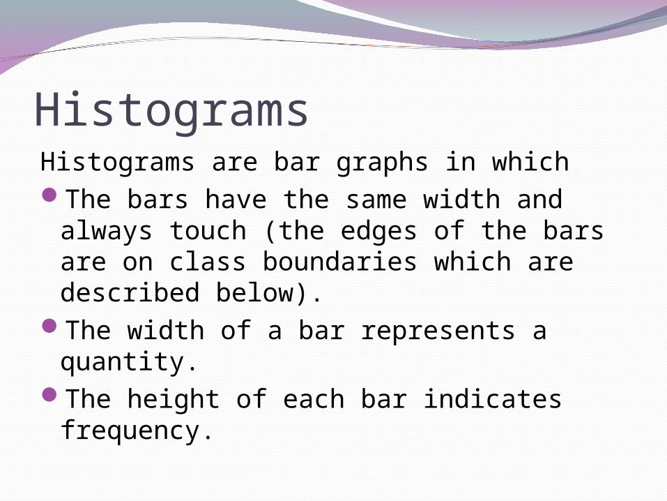
HistogramsHistograms are bar graphs in whichThe bars have the same width and always
touch (the edges of the bars are on class boundaries which are described below).
The width of a bar represents a quantity.The height of each bar indicates
frequency.
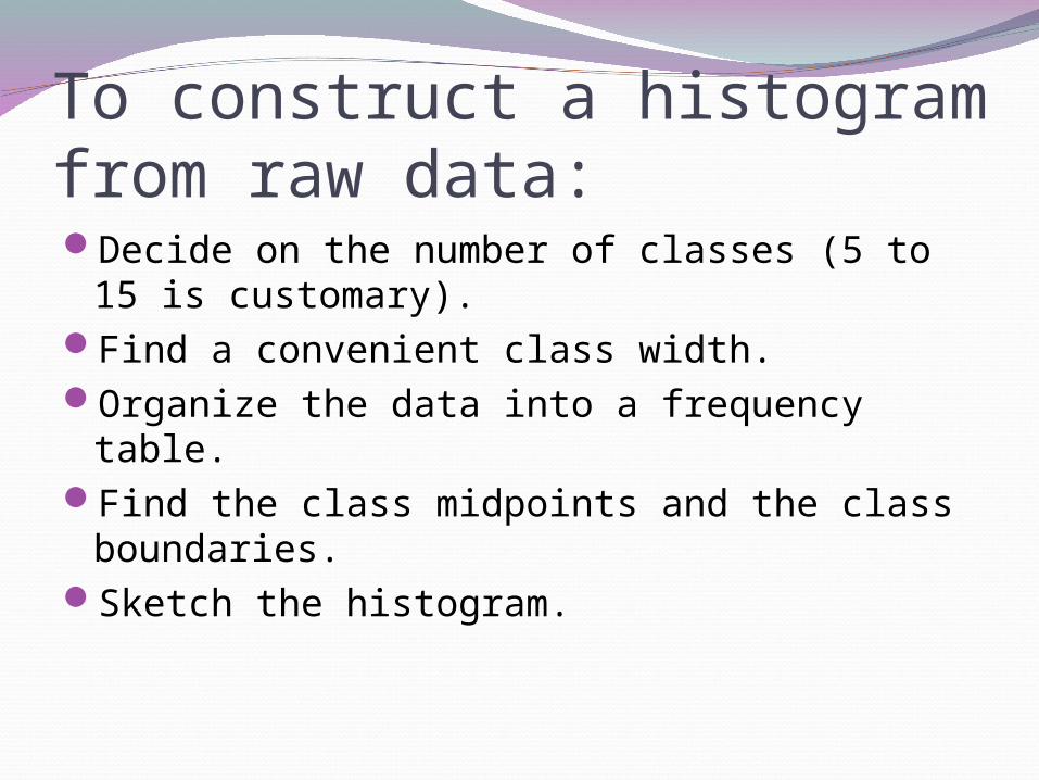
To construct a histogram from raw data:Decide on the number of classes (5 to 15 is
customary).Find a convenient class width.Organize the data into a frequency table.Find the class midpoints and the class
boundaries.Sketch the histogram.

To find Class WidthFirst compute: Largest value - smallest
value Desired number of classes
Increase the value computed to the next highest whole number.
The lower class limit of a class is the lowest data that can fit into the class, the upper class limit is the highest data value that can fit into the class. The class width is the difference between lower class limits of adjacent classes.
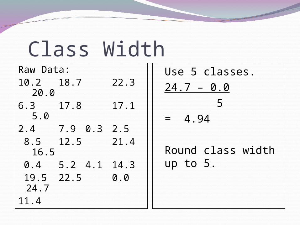
Class WidthRaw Data:10.2 18.7 22.3 20.06.3 17.8 17.1 5.02.4 7.9 0.3 2.5 8.5 12.5 21.4 16.5 0.4 5.2 4.1 14.3 19.5 22.5 0.0 24.711.4
Use 5 classes.24.7 – 0.0 5= 4.94
Round class width up to 5.

Frequency TableDetermine class width.Create the classes. May use smallest data
value as lower limit of first class and add width to get lower limit of next class.
Tally data into classes.Compute midpoints for each class.Determine class boundaries.
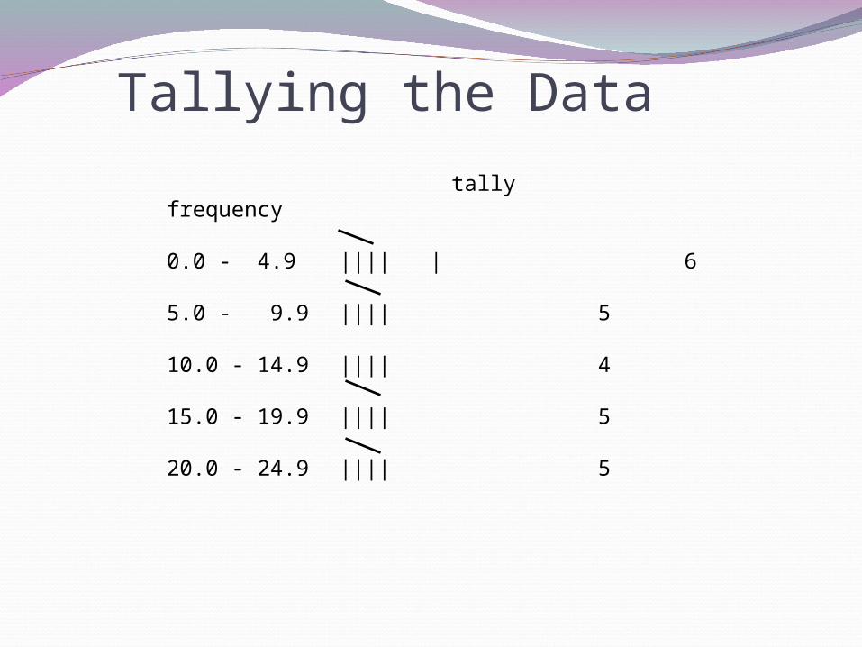
Tallying the Data
tally frequency
0.0 - 4.9 |||| | 6
5.0 - 9.9 |||| 5
10.0 - 14.9 |||| 4
15.0 - 19.9 |||| 5
20.0 - 24.9 |||| 5
Computing Class Width
difference between the lower class limit of one class and the lower class limit of the next class

f class widths
0.0 - 4.9 6 5
5.0 - 9.9 6 5
10.0 - 14.9 4 5
15.0 - 19.9 5 5
20.0 - 24.9 5 5
Finding Class Widths

Computing Class Midpoints
lower class limit + upper class limit 2
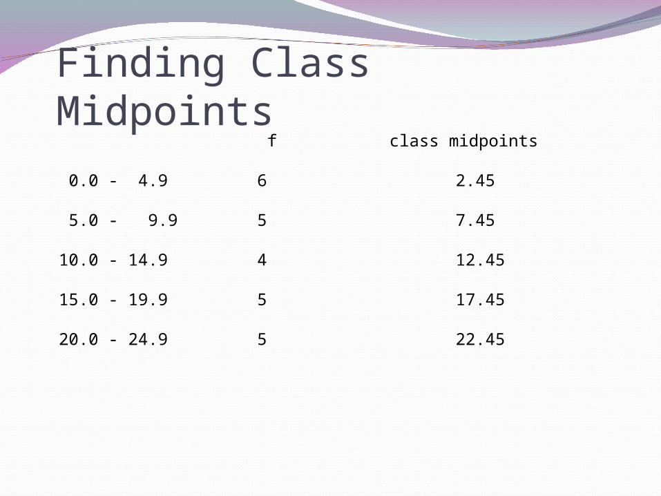
f class midpoints
0.0 - 4.9 6 2.45
5.0 - 9.9 5 7.45
10.0 - 14.9 4 12.45
15.0 - 19.9 5 17.45
20.0 - 24.9 5 22.45
Finding Class Midpoints

Class BoundariesUpper limit of one class + lower limit of next class
2Class boundaries cannot belong to any class. Class boundaries between adjacent classes
are the midpoint between the upper limit of the first class, and the lower limit of the higher class.
Differences between upper and lower boundaries of a given class is the class width.
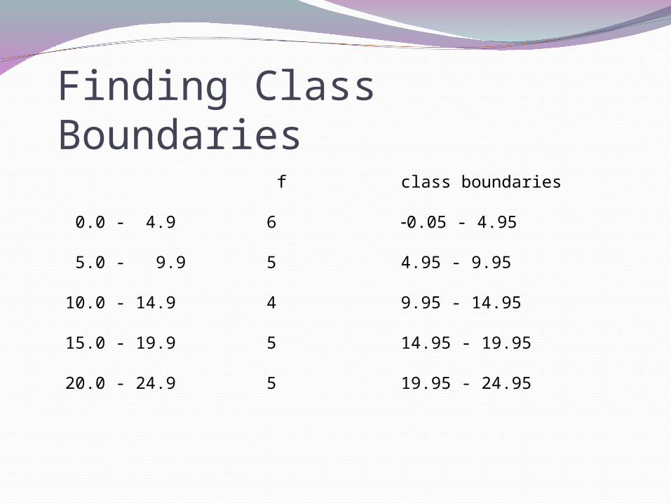
f class boundaries
0.0 - 4.9 6 0.05 - 4.95 5.0 - 9.9 5 4.95 - 9.95
10.0 - 14.9 4 9.95 - 14.95
15.0 - 19.9 5 14.95 - 19.95
20.0 - 24.9 5 19.95 - 24.95
Finding Class Boundaries
f
0.0 - 4.9 6
5.0 - 9.9 5
10.0 - 14.9 4
15.0 - 19.9 5
20.0 - 24.9 5
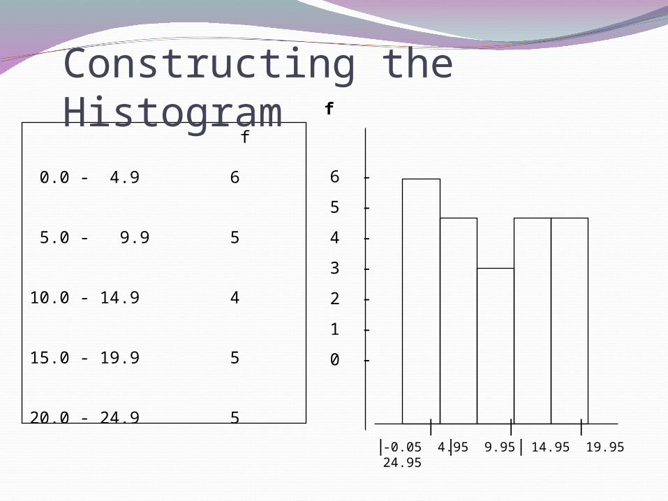
Constructing the Histogram f
| | | | | |
6
5
4
3
2
1
0
-
-
-
-
-
-
-
-0.05 4.95 9.95 14.95 19.95 24.95

Relative FrequenciesThe relative frequency of a class is f/n where
f is the frequency of the class, and n is the total of all frequencies.
Relative frequency tables are like frequency tables except the relative frequency is given.
Relative frequency histograms are like frequency histograms except the height of the bars represent relative frequencies.
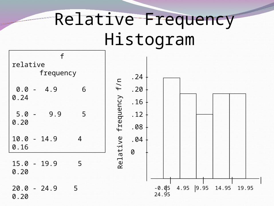
f relative frequency
0.0 - 4.9 6 0.24
5.0 - 9.9 5 0.20
10.0 - 14.9 4 0.16
15.0 - 19.9 5 0.20
20.0 - 24.9 5 0.20
Relative Frequency Histogram
| | | | | |
.24
.20
.16
.12
.08
.04
0
-
-
-
-
-
-
-
-0.05 4.95 9.95 14.95 19.95 24.95
Rela
tive f
requ
ency
f/n
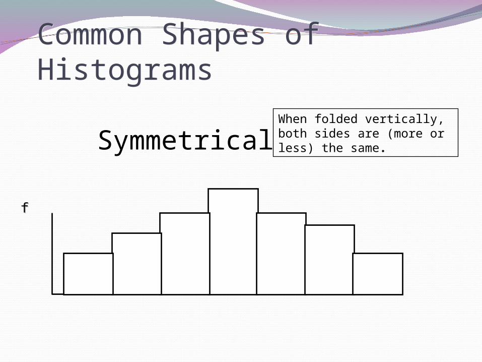
Common Shapes of HistogramsCommon Shapes of Histograms
Symmetrical
ff
When folded vertically, both sides are (more or less) the same.

Common Shapes of HistogramsCommon Shapes of Histograms
Also Symmetrical
ff
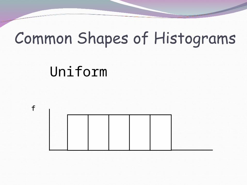
Uniform
ff
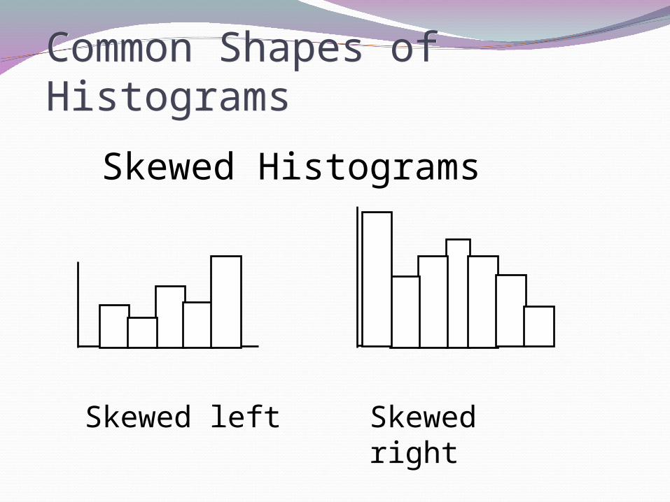
Common Shapes of HistogramsCommon Shapes of Histograms
Skewed Histograms
Skewed left Skewed right
Common Shapes of HistogramsCommon Shapes of Histograms
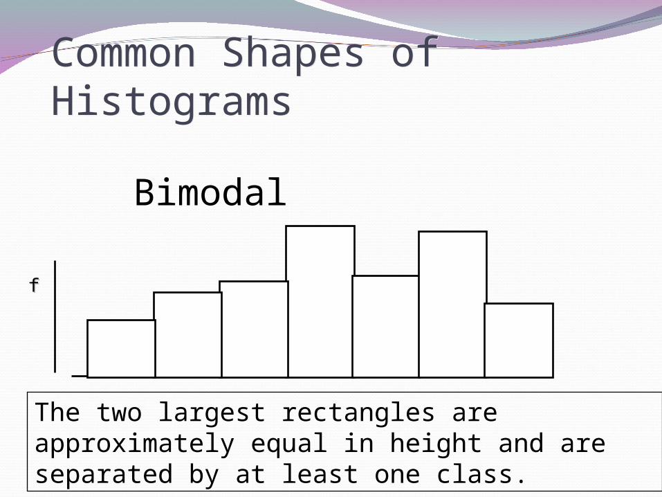
Bimodal
ff
The two largest rectangles are approximately equal in height and are separated by at least one class.

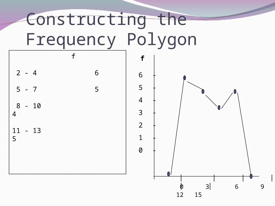
Frequency PolygonA frequency polygon
or line graph emphasizes the continuous rise or fall of the frequencies.
Dots are placed over the midpoints of each class.
Dots are joined by line segments.
Zero frequency classes are included at each end.
f
2 - 4 6
5 - 7 5
8 - 10 4
11 - 13 5
Constructing the Frequency Polygon
f
| | | | | |
6
5
4
3
2
1
0
-
-
-
-
-
-
-
0 3 6 9 12 15
Cumulative Frequencies & OgivesThe cumulative frequency of a class
is the frequency of the class plus the frequencies for all previous classes.
An ogive is a cumulative frequency polygon.
f
Greater than 1.5 20
Greater than 4.5 14
Greater than 7.5 9
Greater than 10.5 5
Greater than 13.5 0
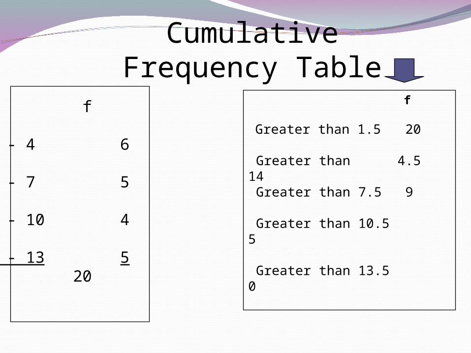
Cumulative Frequency Table
f
2 - 4 6
5 - 7 5
8 - 10 4
11 - 13 5 20

f
Greater than 1.5 20
Greater than 4.5 14
Greater than 7.5 9
Greater than 10.5 5
Greater than 13.5 0
Constructing the Ogive
Cu
mu
lati
ve f
req
uen
cy
| | | | | |
20
15
10
5
0
-
-
-
-
-
1.5 4.5 7.5 10.5 13.5 pounds