Organizational Industrial Organization - HKUccfour/OIO.pdf · 2017-04-21 · Organizational...
97
Introduction Model Market Equilibrium Applications Welfare Extensions Conclusion Organizational Industrial Organization Andy Newman Boston University and CEPR HKU, October 2016 1 / 62
Transcript of Organizational Industrial Organization - HKUccfour/OIO.pdf · 2017-04-21 · Organizational...
Introduction Model Market Equilibrium Applications Welfare Extensions Conclusion
Organizational Industrial Organization
Andy NewmanBoston University and CEPR
HKU, October 2016
1 / 62

Introduction Model Market Equilibrium Applications Welfare Extensions Conclusion
[Industrial Organization] is concerned with how productiveactivities are brought into harmony with society’s demands forgoods and services through some organizing mechanism such as afree market, and how variations and imperfections in the organizingmechanism affect the degree of success achieved by producers insatisfying society’s wants.
– Scherer (1980)
3 / 62
Introduction Model Market Equilibrium Applications Welfare Extensions Conclusion
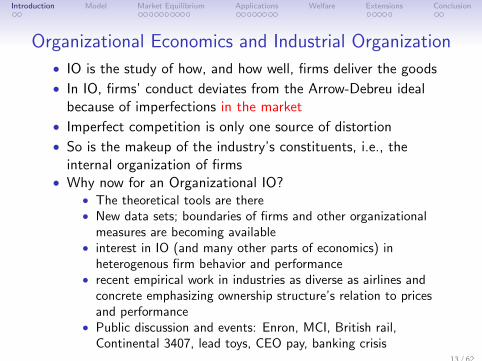
Organizational Economics and Industrial Organization
• IO is the study of how, and how well, firms deliver the goods
• In IO, firms’ conduct deviates from the Arrow-Debreu idealbecause of imperfections in the market
• Imperfect competition is only one source of distortion
• So is the makeup of the industry’s constituents, i.e., theinternal organization of firms
• Why now for an Organizational IO?• The theoretical tools are there• New data sets; boundaries of firms and other organizational
measures are becoming available• interest in IO (and many other parts of economics) in
heterogenous firm behavior and performance• recent empirical work in industries as diverse as airlines and
concrete emphasizing ownership structure’s relation to pricesand performance
• Public discussion and events: Enron, MCI, British rail,Continental 3407, lead toys, CEO pay, banking crisis
4 / 62

Introduction Model Market Equilibrium Applications Welfare Extensions Conclusion
Organizational Economics and Industrial Organization
• IO is the study of how, and how well, firms deliver the goods
• In IO, firms’ conduct deviates from the Arrow-Debreu idealbecause of imperfections in the market
• Imperfect competition is only one source of distortion
• So is the makeup of the industry’s constituents, i.e., theinternal organization of firms
• Why now for an Organizational IO?• The theoretical tools are there• New data sets; boundaries of firms and other organizational
measures are becoming available• interest in IO (and many other parts of economics) in
heterogenous firm behavior and performance• recent empirical work in industries as diverse as airlines and
concrete emphasizing ownership structure’s relation to pricesand performance
• Public discussion and events: Enron, MCI, British rail,Continental 3407, lead toys, CEO pay, banking crisis
5 / 62
Introduction Model Market Equilibrium Applications Welfare Extensions Conclusion
Organizational Economics and Industrial Organization
• IO is the study of how, and how well, firms deliver the goods
• In IO, firms’ conduct deviates from the Arrow-Debreu idealbecause of imperfections in the market
• Imperfect competition is only one source of distortion
• So is the makeup of the industry’s constituents, i.e., theinternal organization of firms
• Why now for an Organizational IO?• The theoretical tools are there• New data sets; boundaries of firms and other organizational
measures are becoming available• interest in IO (and many other parts of economics) in
heterogenous firm behavior and performance• recent empirical work in industries as diverse as airlines and
concrete emphasizing ownership structure’s relation to pricesand performance
• Public discussion and events: Enron, MCI, British rail,Continental 3407, lead toys, CEO pay, banking crisis
6 / 62
Introduction Model Market Equilibrium Applications Welfare Extensions Conclusion
Organizational Economics and Industrial Organization
• IO is the study of how, and how well, firms deliver the goods
• In IO, firms’ conduct deviates from the Arrow-Debreu idealbecause of imperfections in the market
• Imperfect competition is only one source of distortion
• So is the makeup of the industry’s constituents, i.e., theinternal organization of firms
• Why now for an Organizational IO?• The theoretical tools are there• New data sets; boundaries of firms and other organizational
measures are becoming available• interest in IO (and many other parts of economics) in
heterogenous firm behavior and performance• recent empirical work in industries as diverse as airlines and
concrete emphasizing ownership structure’s relation to pricesand performance
• Public discussion and events: Enron, MCI, British rail,Continental 3407, lead toys, CEO pay, banking crisis
7 / 62
Introduction Model Market Equilibrium Applications Welfare Extensions Conclusion
Organizational Economics and Industrial Organization
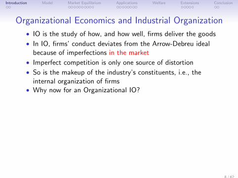
• IO is the study of how, and how well, firms deliver the goods
• In IO, firms’ conduct deviates from the Arrow-Debreu idealbecause of imperfections in the market
• Imperfect competition is only one source of distortion
• So is the makeup of the industry’s constituents, i.e., theinternal organization of firms
• Why now for an Organizational IO?
• The theoretical tools are there• New data sets; boundaries of firms and other organizational
measures are becoming available• interest in IO (and many other parts of economics) in
heterogenous firm behavior and performance• recent empirical work in industries as diverse as airlines and
concrete emphasizing ownership structure’s relation to pricesand performance
• Public discussion and events: Enron, MCI, British rail,Continental 3407, lead toys, CEO pay, banking crisis
8 / 62
Introduction Model Market Equilibrium Applications Welfare Extensions Conclusion
Organizational Economics and Industrial Organization
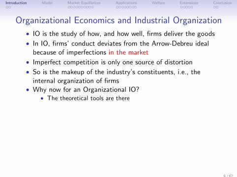
• IO is the study of how, and how well, firms deliver the goods
• In IO, firms’ conduct deviates from the Arrow-Debreu idealbecause of imperfections in the market
• Imperfect competition is only one source of distortion
• So is the makeup of the industry’s constituents, i.e., theinternal organization of firms
• Why now for an Organizational IO?• The theoretical tools are there
• New data sets; boundaries of firms and other organizationalmeasures are becoming available
• interest in IO (and many other parts of economics) inheterogenous firm behavior and performance
• recent empirical work in industries as diverse as airlines andconcrete emphasizing ownership structure’s relation to pricesand performance
• Public discussion and events: Enron, MCI, British rail,Continental 3407, lead toys, CEO pay, banking crisis
9 / 62

Introduction Model Market Equilibrium Applications Welfare Extensions Conclusion
Organizational Economics and Industrial Organization
• IO is the study of how, and how well, firms deliver the goods
• In IO, firms’ conduct deviates from the Arrow-Debreu idealbecause of imperfections in the market
• Imperfect competition is only one source of distortion
• So is the makeup of the industry’s constituents, i.e., theinternal organization of firms
• Why now for an Organizational IO?• The theoretical tools are there• New data sets; boundaries of firms and other organizational
measures are becoming available
• interest in IO (and many other parts of economics) inheterogenous firm behavior and performance
• recent empirical work in industries as diverse as airlines andconcrete emphasizing ownership structure’s relation to pricesand performance
• Public discussion and events: Enron, MCI, British rail,Continental 3407, lead toys, CEO pay, banking crisis
10 / 62
Introduction Model Market Equilibrium Applications Welfare Extensions Conclusion
Organizational Economics and Industrial Organization
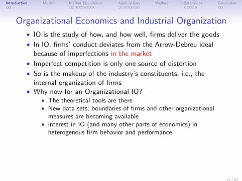
• IO is the study of how, and how well, firms deliver the goods
• In IO, firms’ conduct deviates from the Arrow-Debreu idealbecause of imperfections in the market
• Imperfect competition is only one source of distortion
• So is the makeup of the industry’s constituents, i.e., theinternal organization of firms
• Why now for an Organizational IO?• The theoretical tools are there• New data sets; boundaries of firms and other organizational
measures are becoming available• interest in IO (and many other parts of economics) in
heterogenous firm behavior and performance
• recent empirical work in industries as diverse as airlines andconcrete emphasizing ownership structure’s relation to pricesand performance
• Public discussion and events: Enron, MCI, British rail,Continental 3407, lead toys, CEO pay, banking crisis
11 / 62
Introduction Model Market Equilibrium Applications Welfare Extensions Conclusion
Organizational Economics and Industrial Organization
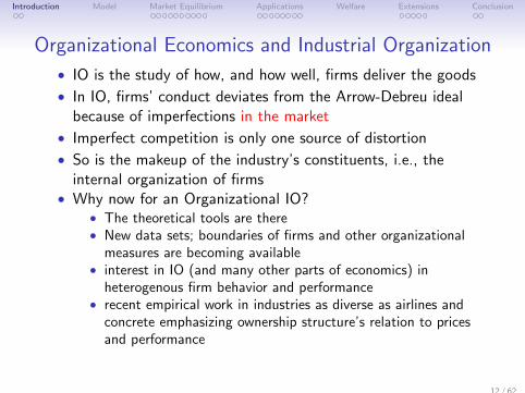
• IO is the study of how, and how well, firms deliver the goods
• In IO, firms’ conduct deviates from the Arrow-Debreu idealbecause of imperfections in the market
• Imperfect competition is only one source of distortion
• So is the makeup of the industry’s constituents, i.e., theinternal organization of firms
• Why now for an Organizational IO?• The theoretical tools are there• New data sets; boundaries of firms and other organizational
measures are becoming available• interest in IO (and many other parts of economics) in
heterogenous firm behavior and performance• recent empirical work in industries as diverse as airlines and
concrete emphasizing ownership structure’s relation to pricesand performance
• Public discussion and events: Enron, MCI, British rail,Continental 3407, lead toys, CEO pay, banking crisis
12 / 62
Introduction Model Market Equilibrium Applications Welfare Extensions Conclusion
Organizational Economics and Industrial Organization
• IO is the study of how, and how well, firms deliver the goods
• In IO, firms’ conduct deviates from the Arrow-Debreu idealbecause of imperfections in the market
• Imperfect competition is only one source of distortion
• So is the makeup of the industry’s constituents, i.e., theinternal organization of firms
• Why now for an Organizational IO?• The theoretical tools are there• New data sets; boundaries of firms and other organizational
measures are becoming available• interest in IO (and many other parts of economics) in
heterogenous firm behavior and performance• recent empirical work in industries as diverse as airlines and
concrete emphasizing ownership structure’s relation to pricesand performance
• Public discussion and events: Enron, MCI, British rail,Continental 3407, lead toys, CEO pay, banking crisis
13 / 62

DECENTRALIZATION VARIES ACROSS FIRMS(Bloom, Sadun, vanReenen, 2012)
Decentralization measure (higher number is more decentralized)
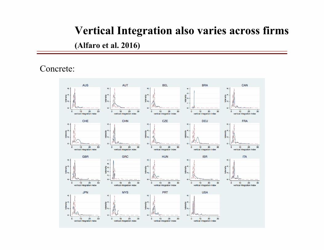
Vertical Integration also varies across firms (Alfaro et al. 2016)
Concrete:
Introduction Model Market Equilibrium Applications Welfare Extensions Conclusion
Questions for an “Organizational Industrial Organization”
• What deviations from the Arrow-Debreu benchmark canimperfections within firms be expected to generate?
• Do these departures differ from those generated byimperfectly competitive product markets? (OE helps IO)
• Two-way street: organization is endogenous, so the marketcould be expected to influence organization (IO helps OE)
• Start with perfect competition so that market imperfectionsdon’t cloud issues
• This leaves open an important issue (future research) namelythe structure of competition is itself endogenous toorganizational design (e.g., firm boundaries)
14 / 62
Introduction Model Market Equilibrium Applications Welfare Extensions Conclusion
Questions for an “Organizational Industrial Organization”
• What deviations from the Arrow-Debreu benchmark canimperfections within firms be expected to generate?
• Do these departures differ from those generated byimperfectly competitive product markets? (OE helps IO)
• Two-way street: organization is endogenous, so the marketcould be expected to influence organization (IO helps OE)
• Start with perfect competition so that market imperfectionsdon’t cloud issues
• This leaves open an important issue (future research) namelythe structure of competition is itself endogenous toorganizational design (e.g., firm boundaries)
15 / 62
Introduction Model Market Equilibrium Applications Welfare Extensions Conclusion
Literature (1)Legros and Newman, ”Incomplete Contracts and Industrial Organization: A Survey”
• Incomplete contracting/ownership: Grossman-Hart (1986);Hart-Moore (1990); Aghion-Bolton (1992)
• Integration as a solution to coordination problems:Alchian-Demsetz (1972), Hart-Moore (2005);Mailath-Postlewaite-Volke (2002); Hart-Holmstrm (2002/10)
• X-inefficiency: Leibenstein (1966), Bertrand-Mullainathan(2003)
16 / 62

Introduction Model Market Equilibrium Applications Welfare Extensions Conclusion
Literature (2)
Effects of markets on organizations and of organizations onmarkets
• Incentives: Hart (1983); Schmidt (1997)
• Monitoring in competitive settings: Legros-Newman (1996)
• Firm boundaries in competitive supplier markets:Legros-Newman (2008)
• Market foreclosure and firm boundaries: Bolton-Whinston(1993)
• Make-Buy decisions with monopolistic competition:Grossman-Helpman (2002)
• Hierarchies: Calvo-Wellisz (1979) and Garicano (2000)
• Delegation and imperfect competition: Marin-Verdier (2008),Alonso-Dessein-Mathouschek (2008)
17 / 62

Introduction Model Market Equilibrium Applications Welfare Extensions Conclusion
Literature (3)
Empirics
• Industry studies on vertical/lateral integration• Airlines: Forbes-Lederman (2009, 2010)• Cement and Ready-Mix Concrete: Hortacsu and Syverson
(JPE 2007)
• Cross Industry studies (e.g. Aghion, Griffith, Zilibotti, 2006)
• Cross-country studies• Other aspects of organization: reporting structures
(Guadalupe-Wulf, 2011); management practice,delegation/decentralization (Bloom, Sadun, vanReenen, 2010,2012)
• Vertical Integration: Acemoglu, Johnson, Mitton (2010);Alfaro et al. (2016)
18 / 62

Introduction Model Market Equilibrium Applications Welfare Extensions Conclusion
”A Price Theory of Vertical and Lateral Integration”Patrick Legros and Andrew Newman
• Look at an “incomplete contracts” model in which productmarket prices interact with organizational design decisions in aperfectly competitive environment
• Prices affect organizational design by affecting the trade-offbetween financial and private motives of managers
• Embed this organizational model into a standardsupply-demand framework
19 / 62
Introduction Model Market Equilibrium Applications Welfare Extensions Conclusion
What We Learn
• Determinants of organizational choices are often to be foundoutside the firm (i.e. in the market)
• In particular, demand matters as well as liquidity and surplusdivision
• Consumers — who are usually absent from organizationtheory — are affected by organizational choices
• An organizational IO can tell us whether the market selects“efficient” organizations.
20 / 62

Introduction Model Market Equilibrium Applications Welfare Extensions Conclusion
Ingredients of a Model
• Efficient production requires coordination; managers disagreeon which way is best (Hart-Holmstrom, 2002/10)
• Non-integration: managers make their decisions separately,and this may lead to inefficient production
• Integration: brings in an additional party (“HQ”) who hasonly monetary motives and will therefore maximize theenterprise’s output by enforcing a common standard
• Supplier and product markets are perfectly competitive
21 / 62

Introduction Model Market Equilibrium Applications Welfare Extensions Conclusion
Results
• Relation between price and organization embodied in supplycurve (the “OAS”): non-integration at low prices, integrationat higher prices
• Changes in price lead to coordinated changes in organization:e.g., an increase in demand may lead to a flurry ofintegration, i.e., a “merger wave.”
• Shocks to some firms (e.g., productivity) propagate and leadto reorganization of “unshocked” firms
• These organizational effects will in turn feed back to quantity,price, and welfare: possibly too little integration at low prices
22 / 62
Introduction Model Market Equilibrium Applications Welfare Extensions Conclusion
Technology
• Two types of supplier: A and B; production requires one ofeach be paired
• Economy has large numbers of each type, with A’soutnumbering the unit measure of B’s
• Large number of HQ’s (more than the number of B’s)
• For each provider, a decision is rendered indicating the way inwhich production is to be carried out.
• A decision a ∈ [0, 1], and B decision b ∈ [0, 1]
• Minimizing output loss requires decisions made in each part ofthe firm should coincide: output is
• 1, with probability 1− (a− b)2
• 0, with remaining probability• outcomes independent across firms
23 / 62

Introduction Model Market Equilibrium Applications Welfare Extensions Conclusion
Managers
• Each supplier run by a risk-neutral manager• A manager’s payoff is y − (1− a)2: “1” is best• B manager’s payoff is y − b2 : “0” is best• y ≥ 0 is income• cost functions reflect differences in the technology managers
run, differences in conduct workforces find convenient, ordisagreement over best ways to manufacture or market product
• A and B managers have zero cash endowments
• HQ’s have zero opportunity cost, preferences y and cashendowments h > 0
24 / 62

Introduction Model Market Equilibrium Applications Welfare Extensions Conclusion
Contracts
• Decisions are not contractible
• Costs are private and non-contractible
• Right to make decisions can be reassigned by contract
• Output generated by the firm is contractible (for monetaryincentives)
• Managers bear the cost of decisions even if they don’t makethem
25 / 62

Introduction Model Market Equilibrium Applications Welfare Extensions Conclusion
Tradeoffs
Change of organization =⇒ change in incentive problem
• Non-integration: managers undervalue coordination, overvalueprivate costs.
• Integration: HQ undervalues managers’ costs, overvaluescoordination.
26 / 62
Introduction Model Market Equilibrium Applications Welfare Extensions Conclusion
Markets
Supplier Market
• B managers match with A managers;
• A’s are on the long side and B’s are on the short side
• HQ market
Contracts
• Ownership structure of the relationship: nonintegration (N) orintegration (I )
• Shares s (endogenous) of managerial revenue P accruing tomanager A, B and HQ if relevant.
• Ex-ante transfers πA, πB from HQ to A,B.
Product Market
• Competitive; demand function is D(P)27 / 62
Introduction Model Market Equilibrium Applications Welfare Extensions Conclusion
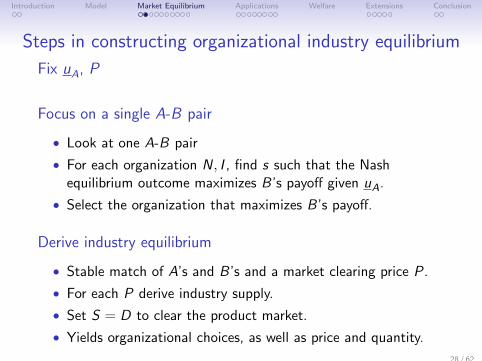
Steps in constructing organizational industry equilibrium
Fix uA, P
Focus on a single A-B pair
• Look at one A-B pair
• For each organization N, I , find s such that the Nashequilibrium outcome maximizes B’s payoff given uA.
• Select the organization that maximizes B’s payoff.
Derive industry equilibrium
• Stable match of A’s and B’s and a market clearing price P.
• For each P derive industry supply.
• Set S = D to clear the product market.
• Yields organizational choices, as well as price and quantity.
28 / 62
Introduction Model Market Equilibrium Applications Welfare Extensions Conclusion
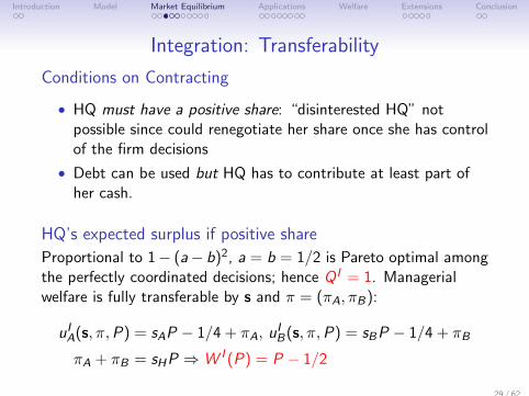
Integration: Transferability
Conditions on Contracting
• HQ must have a positive share: “disinterested HQ” notpossible since could renegotiate her share once she has controlof the firm decisions
• Debt can be used but HQ has to contribute at least part ofher cash.
HQ’s expected surplus if positive share
Proportional to 1− (a− b)2, a = b = 1/2 is Pareto optimal amongthe perfectly coordinated decisions; hence Q I = 1. Managerialwelfare is fully transferable by s and π = (πA, πB):
uIA(s, π,P) = sAP − 1/4 + πA, uI
B(s, π,P) = sBP − 1/4 + πB
πA + πB = sHP ⇒W I (P) = P − 1/2
29 / 62
Introduction Model Market Equilibrium Applications Welfare Extensions Conclusion
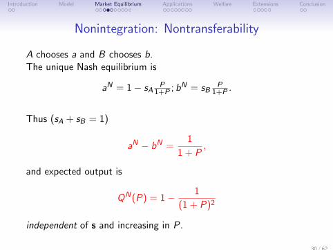
Nonintegration: Nontransferability
A chooses a and B chooses b.The unique Nash equilibrium is
aN = 1− sAP
1+P ; bN = sBP
1+P .
Thus (sA + sB = 1)
aN − bN =1
1 + P,
and expected output is
QN(P) = 1− 1
(1 + P)2
independent of s and increasing in P.
30 / 62
Introduction Model Market Equilibrium Applications Welfare Extensions Conclusion
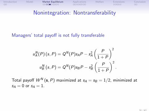
Nonintegration: Nontransferability
Managers’ total payoff is not fully transferable
uNA (P) (s,P) = QN(P)sAP − s2A
(P
1 + P
)2
uNB (s,P) = QN(P)sBP − s2B
(P
1 + P
)2
.
Total payoff W N (s,P) maximized at sA = sB = 1/2, minimized atsA = 0 or sA = 1.
31 / 62

Introduction Model Market Equilibrium Applications Welfare Extensions Conclusion
Comparing Organizations
Total Managerial Payoff Comparison
W N
(1
2,P
)> W I (P)
but W N (0,P) > W I (P) only if P < 1.
Relative Positions depend on price
• For low (< 1) prices non-integration dominates,
• For higher (> 1) prices, the two frontiers cross.
Case uA = 0
Optimal to have sA = 0, sB = 1: B gets W N(0,P) if P < 1 andgets P − 1/2 if P > 1.
32 / 62
Introduction Model Market Equilibrium Applications Welfare Extensions Conclusion
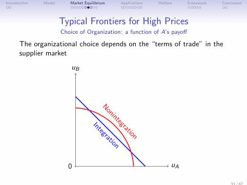
Typical Frontiers for High PricesChoice of Organization: a function of A’s payoff
The organizational choice depends on the “terms of trade” in thesupplier market
0 uA
uB
Integration
Nonintegration
33 / 62
Introduction Model Market Equilibrium Applications Welfare Extensions Conclusion
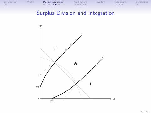
Surplus Division and Integration
0
uB
uA
1
1
0.5
0.5
N
I
I
34 / 62
Introduction Model Market Equilibrium Applications Welfare Extensions Conclusion
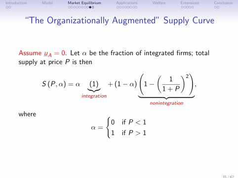
“The Organizationally Augmented” Supply Curve
Assume uA = 0. Let α be the fraction of integrated firms; totalsupply at price P is then
S (P, α) = α (1)︸︷︷︸integration
+ (1− α)
(1−
(1
1 + P
)2)
︸ ︷︷ ︸nonintegration
,
where
α =
{0 if P < 1
1 if P > 1
35 / 62
Introduction Model Market Equilibrium Applications Welfare Extensions Conclusion
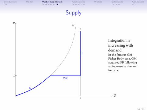
Supply
Q
P
1
I
N
1
N
mix
I
36 / 62
Integration is increasing with demand. In the famous GM-Fisher Body case, GM acquired FB following an increase in demand for cars.
Introduction Model Market Equilibrium Applications Welfare Extensions Conclusion
Application 1: AirlinesForbes-Lederman (2009, 2010)
• Heterogeneity of ownership structures
• Integration more likely on routes that are more valuable (i.e.higher P)
• Airline integration appears to be partly demand driven(movement along the OAS)
37 / 62
Introduction Model Market Equilibrium Applications Welfare Extensions Conclusion
Application 2: Cement, Exogenous HeterogeneityHortacsu-Syverson (2007)
(1) Lower prices with more integration
(2) Integrated firms tend to be more productive
(3) Heterogeneity in ownership structures (for the same“technology”)
• Finding (1) seems at odds with our OAS
• However, we have ignored exogenous heterogeneity until now:supply side effects matter also in this example:(1)-(2) explained if multiple productive levels and marketswith more integrated firms are those with more productivefirms, and therefore have lower prices
• However, still need demand effects for otherwise could notexplain (3)
38 / 62

Introduction Model Market Equilibrium Applications Welfare Extensions Conclusion
Application 2: CementExogenous Heterogeneity
• Proportion z of firms with productivity R > 1 and 1− z withproductivity 1
• D(P) = 34P−1 (at z = 0 equilibrium price is 1 with no
integration)
• R-firms integrate when P > 1/R
• Equilibrium is P(z) ∈ [1/R, 1], decreasing with z
• For P(z) ∈ (1/R, 1), all R-firms are integrated, rest are not:finding (2)
• As z increases from 0, the proportion of integrated firmsincreases, while price decreases: finding (1)
• Let z∗ solve (z∗ < 1): zR + (1− z)(
1− 1(1+P)2
)= 3
4P−1
• Then for z > z∗, P = 1/R, and heterogeneity among highproductivity firms: finding (3).
39 / 62

Introduction Model Market Equilibrium Applications Welfare Extensions Conclusion
Application 3: Organizational Dampening of TechnologicalShocks
Σ(P) =
(1− z)QN(P) + zRQN(RP) if P ≤ 1/R
(1− z)QN(P) + zR if P ∈ (1/R, 1)
1− z + zR if P ≥ 1
Consider two situations: all firms (z0 = 1) with small shock (R0) orfew firms (z < 1) with large shock (R1 > R0), keeping the averageproductivity the same.
zR1 + 1− z = R0 ⇔ z =R0 − 1
R1 − 1
Consider an isoelastic demand P−ε, ε > 1
40 / 62
Introduction Model Market Equilibrium Applications Welfare Extensions Conclusion
Widespread Small ShockReorganization
• Initial equilibrium is at P = 1,Q = 1 (all firms are integrated)
• After the shock, R0 > 1,• the new equilibrium is at P0 = 1/R0
(1/ε)
• this is greater than 1/R0 (since R0 > 1 and ε > 1)
• Hence all firms stay integrated
• total output is R0: Perfect “pass-through” of the aggregateproductivity shock
41 / 62

Introduction Model Market Equilibrium Applications Welfare Extensions Conclusion
Application: Technological ShocksUniform 10% Productivity Increase
Q
P
Sinitial
1
1/1.1
Safter
d
d
ac
42 / 62

Introduction Model Market Equilibrium Applications Welfare Extensions Conclusion
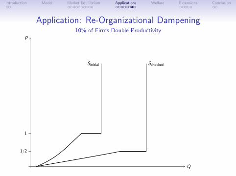
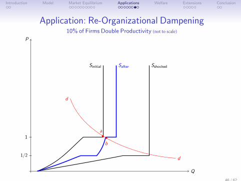
Concentrated Large ShockReorganization of unshocked firms
• Since the price decreases below 1 (more supply!), unshockedfirms shift to non-integration
• The total supply is no more than R0, hence price always atleast 1/R0 > 1/R1
• Hence all shocked firms stay integrated
• Total output is zQN(P) + 1− z < R0: dampening effect ofre-organization
• Under some conditions (4R0 + z < 5) there is completeabsorption: no increase in industry output!
43 / 62
Introduction Model Market Equilibrium Applications Welfare Extensions Conclusion
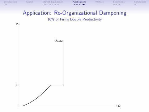
Application: Re-Organizational Dampening10% of Firms Double Productivity
Q
P
Sinitial
1
Sshocked
1/2
Safter
d
d
a
b
44 / 62
Introduction Model Market Equilibrium Applications Welfare Extensions Conclusion
Application: Re-Organizational Dampening10% of Firms Double Productivity
Q
P
Sinitial
1
Sshocked
1/2
Safter
d
d
a
b
45 / 62
Introduction Model Market Equilibrium Applications Welfare Extensions Conclusion
Application: Re-Organizational Dampening 10% of Firms Double Productivity (not to scale)
Q
P
Sinitial
1
Sshocked
1/2
Safter
d
d
a
b
46 / 62

Introduction Model Market Equilibrium Applications Welfare Extensions Conclusion
Summary
• A firm benefiting from a technological shock may notre-organize
• A firm that undergoes a large re-organization need not haveexperienced a change in technology
• Re-organizational dampening may substantially absorb theaggregate benefit of heterogenous technological change
47 / 62

Introduction Model Market Equilibrium Applications Welfare Extensions Conclusion
Welfare
DefinitionAn equilibrium is ownership efficient if it is not possible to increasetotal welfare by changing firms’ ownership structures.
48 / 62
Introduction Model Market Equilibrium Applications Welfare Extensions Conclusion
WelfareSecond-Best Efficiency
Costs
• With non-integration, expected output is Q = 1− (1− b)2,
hence the managerial cost is c(Q) =(1−√
1− Q)2
• For manager B, the solution to maxb(1− (1− b)2)r − b2 isthen the same as the solution to maxQ Qr − c(Q).
• It follows that along the graph(r ,QN(r)
), we have
r = c ′(QN(r))
• For integration, let r = 1; raising the probability of integratingby dα raises the expected output by (1− 3
4)dα and the costby (12 −
14)dα, so c ′(Q) = 1
49 / 62

Introduction Model Market Equilibrium Applications Welfare Extensions Conclusion
Welfare
Second-Best Efficiency
When managers have full residual claim on revenues, equilibria areownership efficient. Supply and marginal cost schedules coincide inequilibrium.
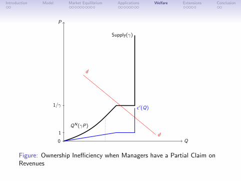
Managerial Firms
• Managers internalize only a fraction γ of the firm’s profits
• Output if price is P under non-integration is QN(γP)
• Main consequence: price-expected output schedule does notcoincide with marginal cost anymore.
50 / 62
Introduction Model Market Equilibrium Applications Welfare Extensions Conclusion
0 Q
P
QN(γP)
Supply(γ)
1/γ
1
d
d
c ′(Q)
ODWL
Figure: Ownership Inefficiency when Managers have a Partial Claim onRevenues
51 / 62

Introduction Model Market Equilibrium Applications Welfare Extensions Conclusion
0 Q
P
QN(γP)
Supply(γ)
1/γ
1
d
d
c ′(Q)
ODWL
Figure: Ownership Inefficiency when Managers have a Partial Claim onRevenues
52 / 62

Introduction Model Market Equilibrium Applications Welfare Extensions Conclusion
Proposition
Suppose that γ < 1. Then there is a generic set of demandsleading to equilibria that are ownership inefficient
• In fact, heterogeneity implies ownership inefficiency
• The set of inefficient equilibrium prices is an interval
Demand Elasticity
• The more elastic market demand is, the larger is the ODWL
• Opposite relationship with market power: there the moreelasticity is the lower is the DWL.
53 / 62

Introduction Model Market Equilibrium Applications Welfare Extensions Conclusion
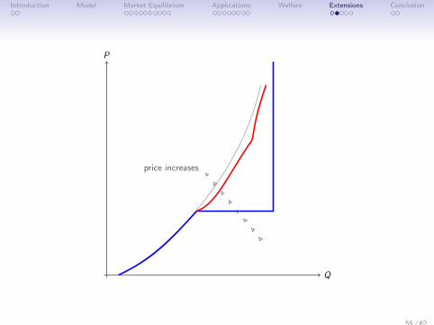
Extension 1: Cash Endowments
• Allows a type A manager to pay the B with cash
• Weakly raises willingness to pay (so high liquidity A’s arematched), but also pushes choice towards nonintegration(since more efficient for managers).
54 / 62
Introduction Model Market Equilibrium Applications Welfare Extensions Conclusion
Q
P
price increases
55 / 62
Introduction Model Market Equilibrium Applications Welfare Extensions Conclusion
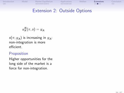
Extension 2: Outside Options
uNA (π, s) = uA
s(π; uA) is increasing in uA:non-integration is moreefficient.
Proposition
Higher opportunities for thelong side of the market is aforce for non-integration.
Q
P
uA ↑
price increases
• Application: Mattel and lead toys (Conconi, Legros, andNewman (2012), JIntE)
56 / 62

Introduction Model Market Equilibrium Applications Welfare Extensions Conclusion
Extension 2: Outside Options
uNA (π, s) = uA
s(π; uA) is increasing in uA:non-integration is moreefficient.
Proposition
Higher opportunities for thelong side of the market is aforce for non-integration. Q
P
uA ↑
price increases
• Application: Mattel and lead toys (Conconi, Legros, andNewman (2012), JIntE)
57 / 62
Introduction Model Market Equilibrium Applications Welfare Extensions Conclusion
Extension 3: Scale
• Can choose f (l) at cost wl and get revenue f (l)P
• Integrated firms behave like “neoclassical firms”: f ′(l I )P = w
• Non-integrated firms behave like “non-neoclassical firms”:QN(Pf (lN)− wlN)f ′(lN)P = w
• Integrated firms have a larger scale: l I > lN
• Similar analysis with other inputs, e.g. workforce/managerialability
• Co-variation of size, workforce quality, and integration.
58 / 62
Introduction Model Market Equilibrium Applications Welfare Extensions Conclusion
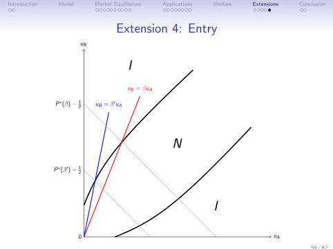
Extension 4: Entry
0
uB
uA
N
I
I
uB = βuA
uB = β′uAP∗(β)− 12
P∗(β′)− 12
59 / 62

Some Evidence (Alfaro et al. 2016)
Questions from Different Fields:
• Organizational Economics What determines Vertical Integration (VI)?
– “technological” determinants such as complementarities among assets or adaptation frequency (Coase 1937, Williamson 1975, SGrossman-Hart 1986, Holmström-Milgrom 1991)
– “pecuniary” or market effects (McLaren 2000; Grossman-Helpman 2002;Legros-Newman 2008, 2013)
• Industrial Organization What is the effect of VI on product prices?
– It raises them (foreclosure theories): motivates “divestment” policy (e.g. in gasoline, beer)
– It lowers them (efficiency theories; c.f. the technological theories from OE above)
– Either way, causality runs from VI to prices
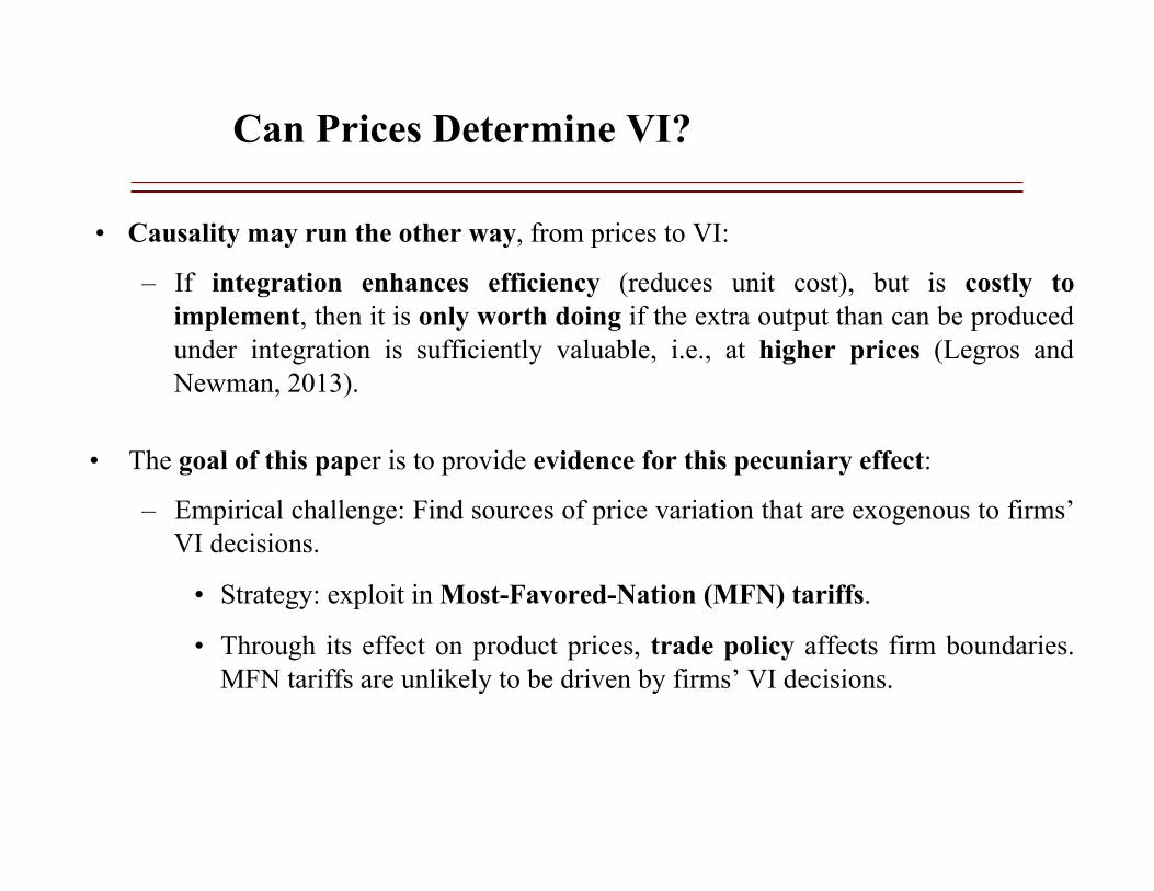
Can Prices Determine VI?
• Causality may run the other way, from prices to VI:
– If integration enhances efficiency (reduces unit cost), but is costly to implement, then it is only worth doing if the extra output than can be produced under integration is sufficiently valuable, i.e., at higher prices (Legros and Newman, 2013).
• The goal of this paper is to provide evidence for this pecuniary effect:
– Empirical challenge: Find sources of price variation that are exogenous to firms’ VI decisions.
• Strategy: exploit in Most-Favored-Nation (MFN) tariffs.
• Through its effect on product prices, trade policy affects firm boundaries. MFN tariffs are unlikely to be driven by firms’ VI decisions.

Empirical Strategy: MFN Tariffs
• MFN principle (GATT article I): countries cannot discriminate between trading partners:– If a country grants a special favor to another, it must do the same for all other members– Tariff bounds vary substantially both across sectors within countries and across
countries for a given sector.
• Long rounds of multilateral trade negotiations: at the end of each round, governments commit not to exceed certain tariff rates; tariff bindings can only be renegotiated in a new round of negotiations.– MFN tariffs are persistent, significantly more so than integration choices.
• They must be applied in a non-discriminatory manner to imports from all countries, which severely limits negotiators’ flexibility to respond to lobbying.– If they respond to short-term political pressure, governments resort to other measures
for regulating imports, such as anti-dumping and countervailing duties (e.g. Finger, Hall and Nelson, 1982).

Empirical Strategy: Approaches
• Empirical analysis of the organizational effects of tariffs
– We construct firm-level vertical integration indices for a large set of countries
• We exploit cross-country and cross-sectoral variation in 2004 applied MFN tariffs
– Vertical integration of firms in 2004: MNF tariffs outcome of the eight-year Uruguay Round of trade negotiation that was completed ten years earlier.
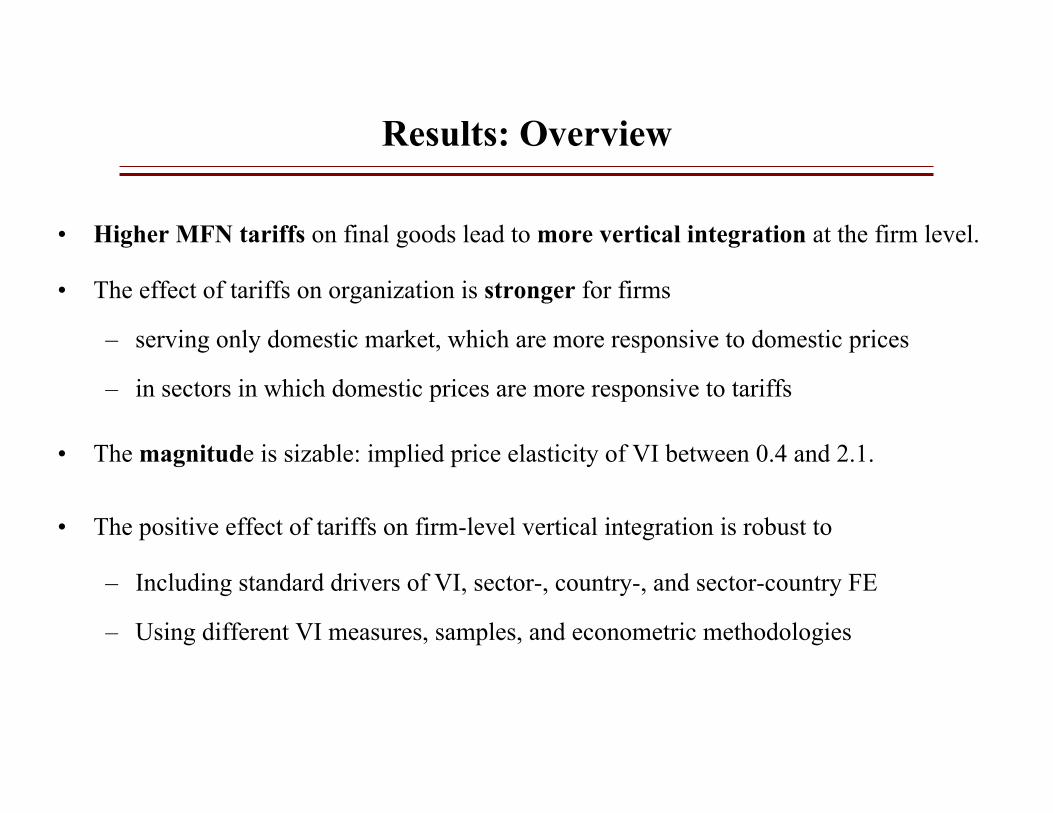
Results: Overview
• Higher MFN tariffs on final goods lead to more vertical integration at the firm level.
• The effect of tariffs on organization is stronger for firms
– serving only domestic market, which are more responsive to domestic prices
– in sectors in which domestic prices are more responsive to tariffs
• The magnitude is sizable: implied price elasticity of VI between 0.4 and 2.1.
• The positive effect of tariffs on firm-level vertical integration is robust to
– Including standard drivers of VI, sector-, country-, and sector-country FE
– Using different VI measures, samples, and econometric methodologies
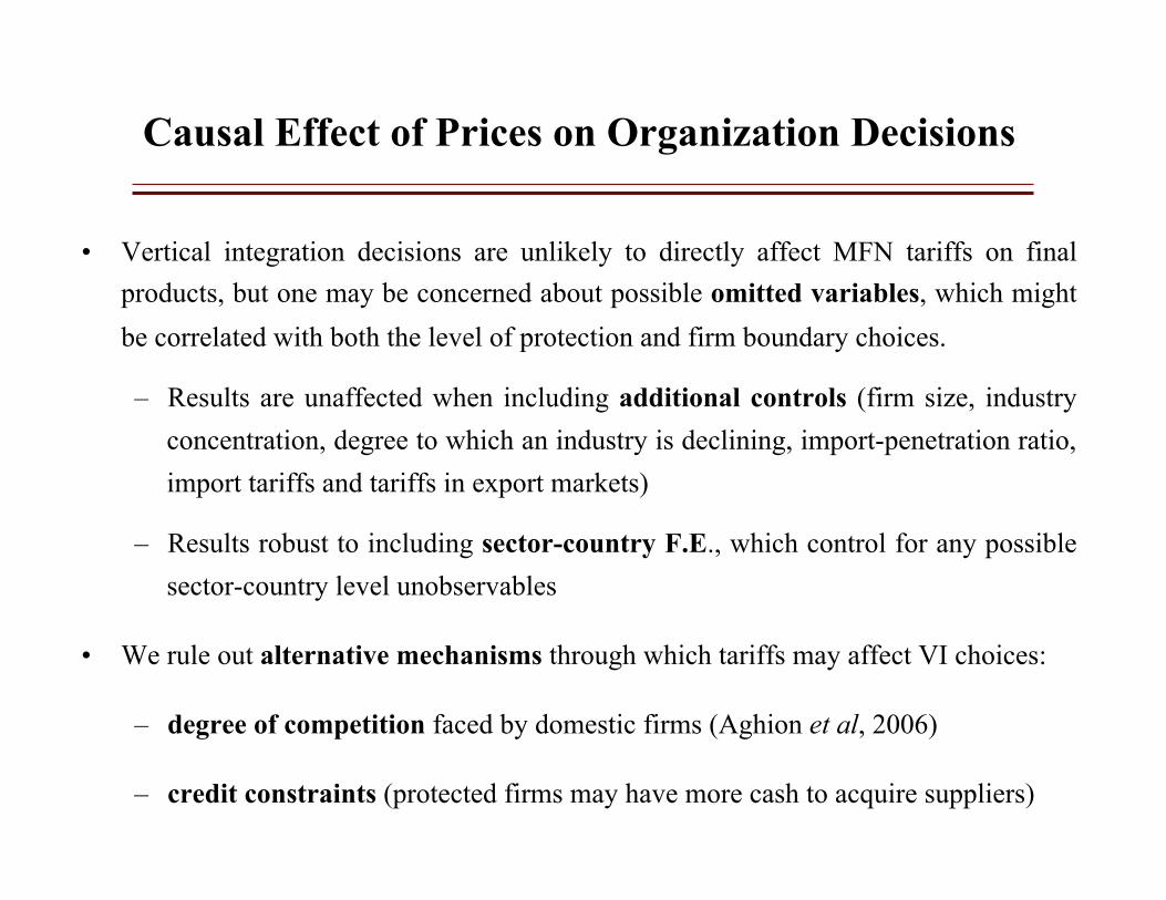
Causal Effect of Prices on Organization Decisions
• Vertical integration decisions are unlikely to directly affect MFN tariffs on final products, but one may be concerned about possible omitted variables, which might be correlated with both the level of protection and firm boundary choices.
– Results are unaffected when including additional controls (firm size, industry concentration, degree to which an industry is declining, import-penetration ratio, import tariffs and tariffs in export markets)
– Results robust to including sector-country F.E., which control for any possible sector-country level unobservables
• We rule out alternative mechanisms through which tariffs may affect VI choices:
– degree of competition faced by domestic firms (Aghion et al, 2006)
– credit constraints (protected firms may have more cash to acquire suppliers)
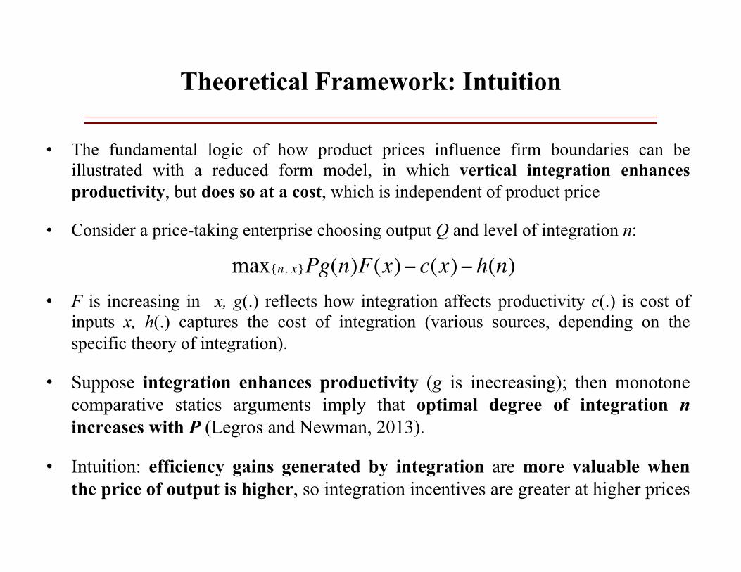
Theoretical Framework: Intuition
• The fundamental logic of how product prices influence firm boundaries can be illustrated with a reduced form model, in which vertical integration enhances productivity, but does so at a cost, which is independent of product price
• Consider a price-taking enterprise choosing output Q and level of integration n:
• F is increasing in x, g(.) reflects how integration affects productivity c(.) is cost of inputs x, h(.) captures the cost of integration (various sources, depending on the specific theory of integration).
• Suppose integration enhances productivity (g is inecreasing); then monotone comparative statics arguments imply that optimal degree of integration n increases with P (Legros and Newman, 2013).
• Intuition: efficiency gains generated by integration are more valuable when the price of output is higher, so integration incentives are greater at higher prices
max{n, x}Pg(n)F(x)− c(x)− h(n)

Import tariffs and vertical integration
• To verify this prediction, we could simply regress VI measures on industry prices
– Problem: distinguishing this view (higher prices → more vertical integration) from market-foreclosure theories (vertical integration → higher prices)
• Trade policy generates an exogenous source of price variation:
– import tariffs affect prices and are unlikely to be driven by firms’ vertical integration decisions
• Consider an import-competing industry composed by many price-taking firms within a small open economy. Denote with P* the world market-clearing price
– An ad-valorem tariff increases the domestic price to P = (1 + t) P*
• By raising the domestic price, the introduction of an import tariff increases the gains from integration for domestic firms, leading them to choose a higher n
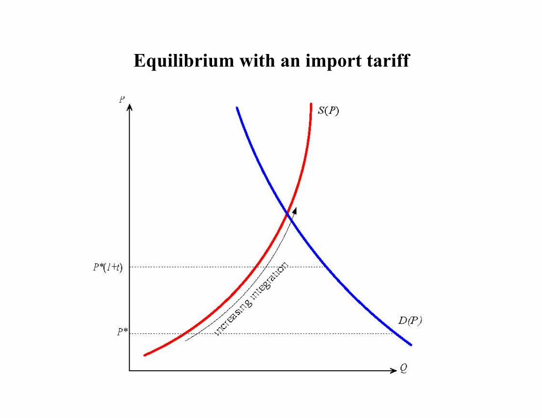
Equilibrium with an import tariff
Import tariffs and vertical integration
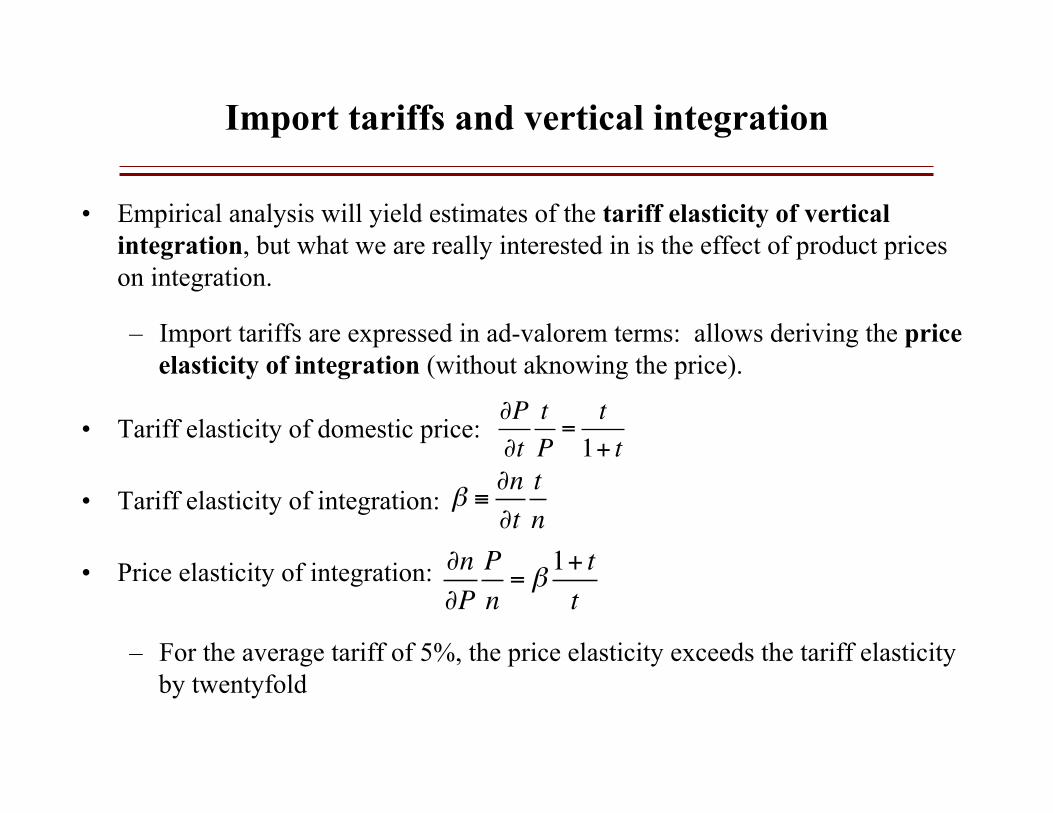
• Empirical analysis will yield estimates of the tariff elasticity of vertical integration, but what we are really interested in is the effect of product prices on integration.
– Import tariffs are expressed in ad-valorem terms: allows deriving the price elasticity of integration (without aknowing the price).
• Tariff elasticity of domestic price:
• Tariff elasticity of integration:
• Price elasticity of integration:
– For the average tariff of 5%, the price elasticity exceeds the tariff elasticity by twentyfold
∂P∂t
tP=
t1+ t
β ≡∂n∂t
tn
∂n∂P
Pn= β
1+ tt
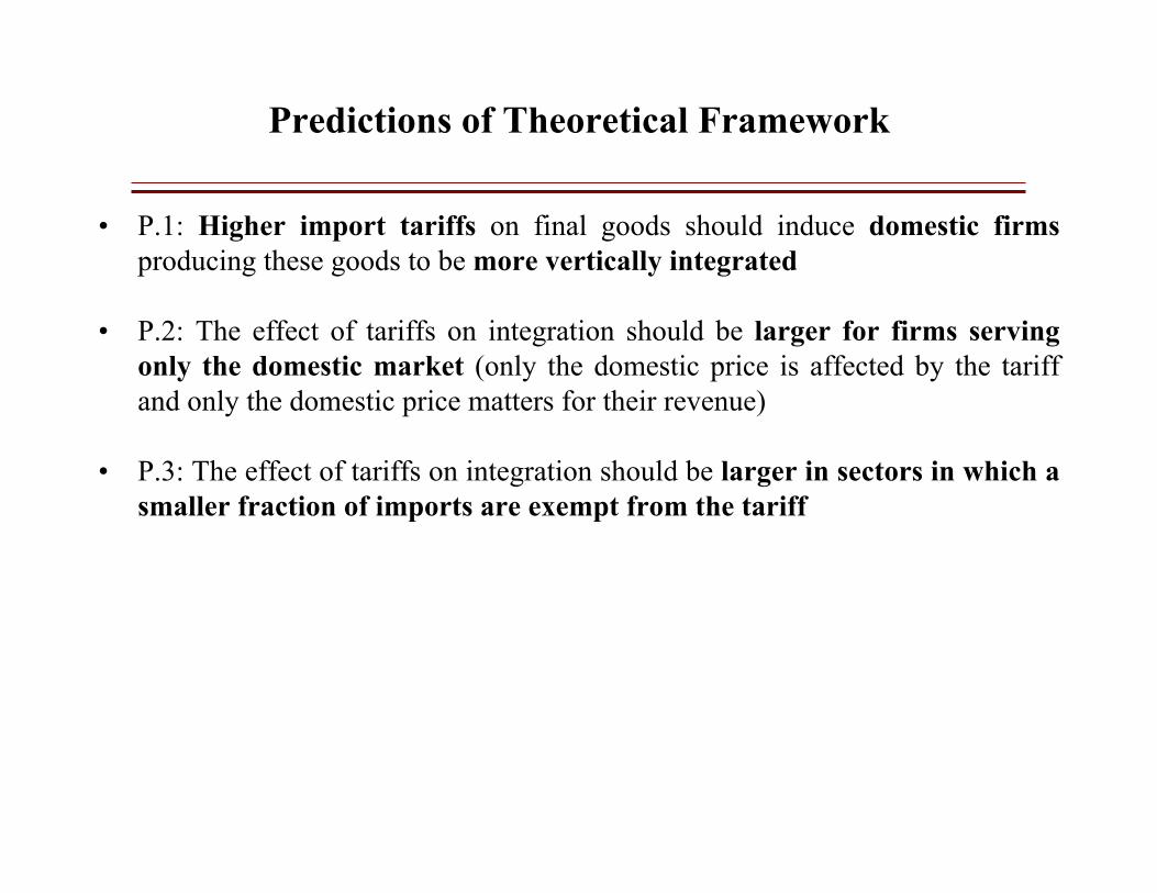
Predictions of Theoretical Framework
• P.1: Higher import tariffs on final goods should induce domestic firms producing these goods to be more vertically integrated
• P.2: The effect of tariffs on integration should be larger for firms serving only the domestic market (only the domestic price is affected by the tariff and only the domestic price matters for their revenue)
• P.3: The effect of tariffs on integration should be larger in sectors in which a smaller fraction of imports are exempt from the tariff

Empirical strategy
• We exploit cross-country and cross-sectoral variation in 2004 applied MFN tariffs:
– Outcome of long-term multilateral negotiations (Uruguay Round:1986-1994)
– GATT/WTO members commit not to exceed agreed tariff bounds; special favors
granted to one country have to granted to all others (GATT Article I)
– Less responsive to political pressure than other trade policies (e.g., anti-dumping)
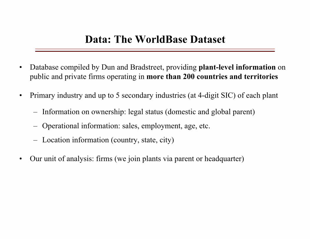
Data: The WorldBase Dataset
• Database compiled by Dun and Bradstreet, providing plant-level information onpublic and private firms operating in more than 200 countries and territories
• Primary industry and up to 5 secondary industries (at 4-digit SIC) of each plant
– Information on ownership: legal status (domestic and global parent)
– Operational information: sales, employment, age, etc.
– Location information (country, state, city)
• Our unit of analysis: firms (we join plants via parent or headquarter)

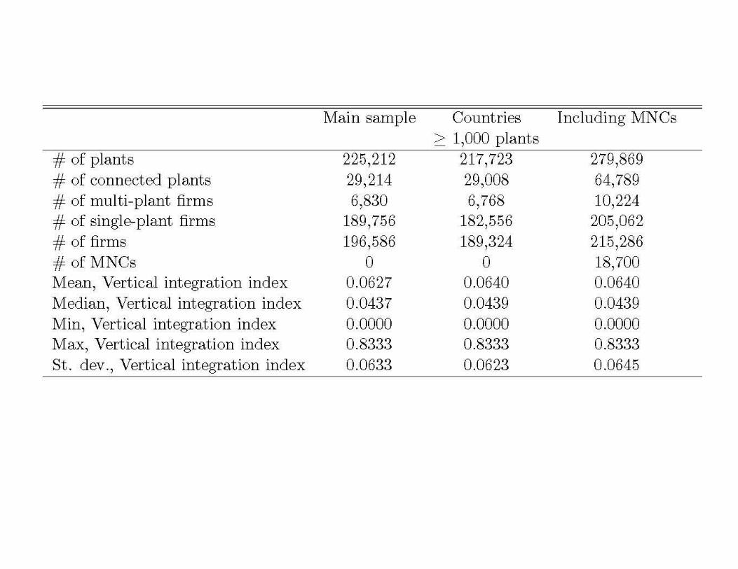
The WorldBase Dataset: Sample
• Main analysis: focus on manufacturing sector (2000-3999), excluding
– Countries/territories with less than 80 observations
– Countries/territories that are not in the WTO
– Firms with less than 20 employees or no SIC codes
• Theory less apt for self employment/collection differences.
– We focus on firms located in one country
• MNCs (relevant price/tariff hard to identify, strategic behavior)
• Robustness with various subsamples (including multinationals, excludingcountries with less than 1000 observations, OECD countries, etc.)

Vertical Integration Index
• To measure vertical integration, we combine information on firms’ production activities (plants aggregated at the firm level) with data from US input-output tables (Fan and Lang, 2000; Acemoglu et al. 2009, Alfaro and Charlton, 2009).
– Firm-level vertical integration indices: fraction of inputs used in the production of a firm’s final good that can be produced in house.
• We match US 4-digit SIC codes for each firm with the 6-digit IO codes, using theBEA’s concordance guide (random matching when multiple).
• The IO coefficients represent the dollar value of inputs to produce one dollar ofoutput (opportunity for vertical integration between sectors i and j).
• Unit of observation: all plants belonging to the same firm (all plants that report to the same headquarter).

Vertical Integration Index
• For a Japanese plant active in automobiles (59.0301), automotive stampings(41.0201) and miscellaneous plastic products (32.0400), its IOij coefficients are
• The IOij coefficient for stampings to autos indicates that 7.8 cents worth of automotive stampings are required to produce a dollar’s output of autos.
• A firm’s VI index: sum of IOij for each industry.
– 12.3 cents worth of the inputs required to make autos can be produced within this plant (measures the fraction of inputs used in the production of the final good that can be produced in house).
Output (j)
Input (i)
Autos Stampings Plastics
Autos 0.0043 0.000 0.0000
Stampings 0.0780 0.0017 0.0000
Plastics 0.0405 0.0024 0.0560
SUM 0.1228 0.0041 0.0560
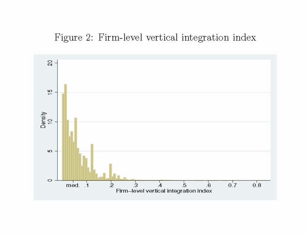

Heterogeneity in VI across countries
Ready-Mix Concrete:
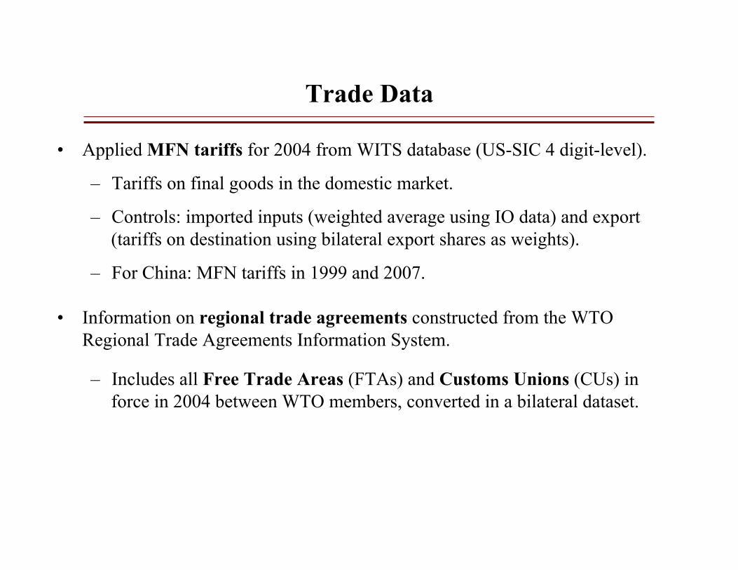
Trade Data
• Applied MFN tariffs for 2004 from WITS database (US-SIC 4 digit-level).
– Tariffs on final goods in the domestic market.
– Controls: imported inputs (weighted average using IO data) and export (tariffs on destination using bilateral export shares as weights).
– For China: MFN tariffs in 1999 and 2007.
• Information on regional trade agreements constructed from the WTO Regional Trade Agreements Information System.
– Includes all Free Trade Areas (FTAs) and Customs Unions (CUs) in force in 2004 between WTO members, converted in a bilateral dataset.

Other Variables • Firm-level (WorldBase)
– Domesticf = 1 if the firm does not report exporting– Sizef: firm-level employment instrumented with sector-country dummies– Labor productivityf : sales/employment instrumented with sector-country dummies– MNCf = 1 if the firm has plants in more than one country
• Sector-level– Capital intensityk: log capital expenditures/value added (Bartelsmann and Gray, 2000)– Herfindahlk,c index based on firms’ sales in a given country and sector (WorldBase)– Decliningk,c,: = (-) emp. growth in industry-country1988-1994 (UNIDO)– Import-competingk,c = log(imports/exports) (Comtrade)– Homogeneous1k = 1, homogeneous according Rauch (1999)– Homogeneous2k =1, import demand elasticity > country median (Broda et al, 2006)
• Country-level and bilateral– Legal qualityc: index of the quality of legal institutions (Kaufmann et al, 2003)– Financial developmentc: domestic credit to private sector % GDP (Beck et al, 2006)– GDPc and GDP per capitac, Differences in GDPcc (WB, WDI)– Colonial relationshipcc’, Contiguitycc’, Common languagecc’ (from CEPII)


Tariffs and Vertical Integration
• To assess validity of our first prediction, we estimate the panel regression model:
Vf,k,c= α + β1MFNk,c+ Xf,k,c+ δc+ δk +εf,k,c
• Dependent variable: Log of (1+ VI index of firm f in country c, with primary sector k).
• Controls:
– Log (1+ MFN tariff applied by country c in sector k).
– Interactions between sector and country characteristics – Country fixed effects (δc ).
– Sector fixed effects at the 4-digit SIC level (δk ).
• Standard errors clustered at the sector-country level (tariffs vary at the sector-country level, dependent variable varies at the firm level).
• To assess the validity of the second and third predictions, we include interactions between the MFN tariff and the variables Domesticf and MFNsharek,,c
– Use country-sector fixed effects in Domesticf*MFNk,c regression

Tariffs and Vertical Integration
(1) (2) (3) (4) (5)
Tariffk,c 0.0203*** 0.0202*** 0.0034 0.0035 (0.0061) (0.0060) (0.0088) (0.0086)
Domes:cf -‐0.0926*** -‐0.0923*** -‐0.0880*** (0.0108) (0.0109) (0.0092)
Tariffk,c× Domes:cf 0.0214*** 0.0212*** 0.0189*** (0.0054) (0.0054) (0.0046)
MFN Sharek,c
Tariffk,c × MFN Sharek,c
Capital Intensityk 0.0322** 0.0321** × Financial Developmentc (0.0142) (0.0144) Capital Intensityk -‐0.0833 -‐0.0823 × Legal Qualityc (0.0564) (0.0573)
# Observa:ons 196,586 196,586 196,586 196,586 196,586 # Sectors 386 386 386 386 R2 0.117 0.117 0.119 0.119 0.002 Sector FE YES YES YES YES NO Country FE YES YES YES YES NO Sector-‐Country FE NO NO NO NO YES
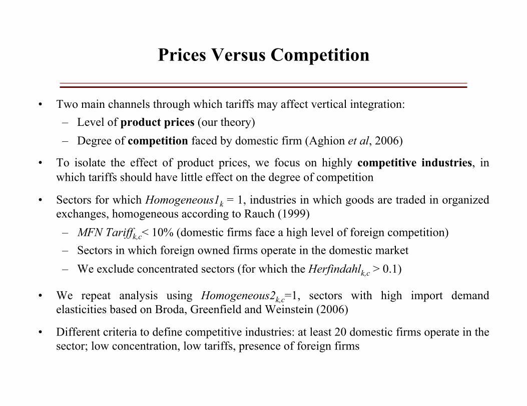
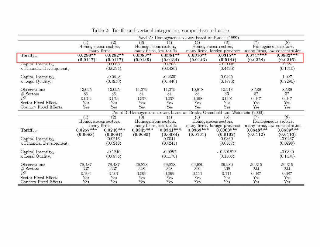
Prices Versus Competition
• Two main channels through which tariffs may affect vertical integration:– Level of product prices (our theory)– Degree of competition faced by domestic firm (Aghion et al, 2006)
• To isolate the effect of product prices, we focus on highly competitive industries, in which tariffs should have little effect on the degree of competition
• Sectors for which Homogeneous1k = 1, industries in which goods are traded in organized exchanges, homogeneous according to Rauch (1999) – MFN Tariffk,c< 10% (domestic firms face a high level of foreign competition)– Sectors in which foreign owned firms operate in the domestic market– We exclude concentrated sectors (for which the Herfindahlk,c > 0.1)
• We repeat analysis using Homogeneous2k,c=1, sectors with high import demand elasticities based on Broda, Greenfield and Weinstein (2006)
• Different criteria to define competitive industries: at least 20 domestic firms operate in the sector; low concentration, low tariffs, presence of foreign firms


Credit constraints
• Another possible explanation for our results relies on credit constraints: protected firms may have more disposable cash to acquire their suppliers
• If this is the reason behind the positive impact of tariffs on vertical integration, the effect should be stronger in countries and sectors in which credit constraints are more severe
• We have interacted the tariff variable with the inverse of the measure Financial Development and with a standard measure of Financial dependence (including the interaction terms separately or together, including a triple interaction between tariffs, financial dependence and the inverse of financial development)
• In all specifications, the interaction terms were insignificant and the sign and significance of the tariff coefficient was unaffected.

Including additional controls
• Possible concerns: – Tariffs that firms face in export markets and tariffs on imported inputs can
be correlated with tariffs on final products and may also affect integration – Large and more productive firms in concentrated industries could be more
effective at lobbying for protection and may also be more vertically integrated – Declining industries tend to be more protected and may also be more integrated
• Results are unaffected when including these additional controls in our analysis: – Firm size and labor productivity – Industry concentration – Input tariffs and export tariffs – Degree to which an industry is declining – Import-penetration ration


Additional Robustness
• Different samples:
– Excluding firms that existed pre-1994
– Including multinational firms, with plants in more than one country
– Excluding countries with less than 1000 observations
– Focusing on OECD countries only
– Excluding the United States.

Additional Robustness Checks
• Alternative measure of vertical integration, constructed based on all the firm's activities rather than its primary activity.
• Including multinational firms (primary activity of the respective domestic ultimate to identify the relevant tariff).
• Excluding countries with less than 1,000 plants that are part of firms with at least 20 employees.
• Different econometric methodologies: Poisson quai-maximum likelihood estimator, alternative clustering of standard errors (at sector and at country level)
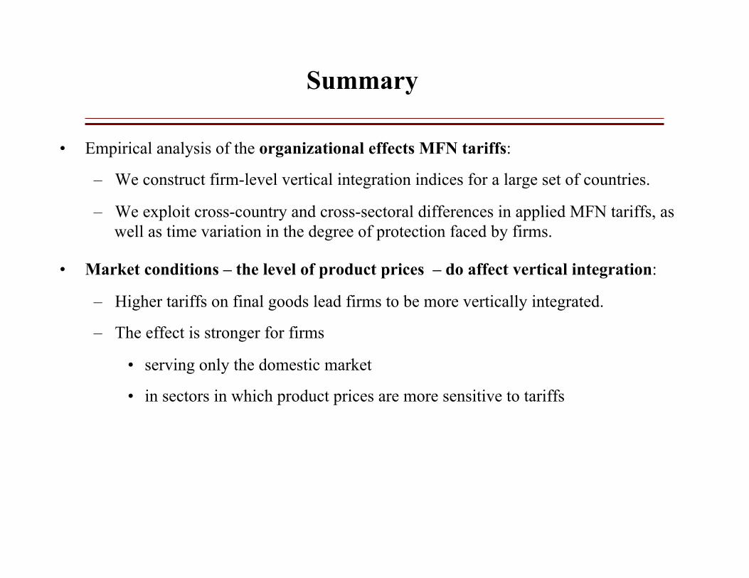
Summary
• Empirical analysis of the organizational effects MFN tariffs:
– We construct firm-level vertical integration indices for a large set of countries.
– We exploit cross-country and cross-sectoral differences in applied MFN tariffs, aswell as time variation in the degree of protection faced by firms.
• Market conditions – the level of product prices – do affect vertical integration:
– Higher tariffs on final goods lead firms to be more vertically integrated.
– The effect is stronger for firms
• serving only the domestic market
• in sectors in which product prices are more sensitive to tariffs

Implications for Policy
• Positive correlations between prices and VI have been observed in many industries:
– Report on the beer industry by the British Monopolies and Mergers Commission
found higher retail prices in integrated than non-integrated pubs (Slade, 1998)
– Increases in gasoline prices in California in the 1990’s were associated with
increases in the number of vertically integrated gasoline stations (Hastings, 2004)
• Policymakers appear to have drawn a causal inference from this correlation, that
vertical integration causes higher prices, in line with market foreclosure theories.
• Positive correlations may be consistent with perfect competition.

Introduction Model Market Equilibrium Applications Welfare Extensions Conclusion
Conclusion
Demand Matters for OrganizationsCoordination device, “clustering” of organizational changes. Prices mayincrease following entry of low cost suppliers. Shocks propagate.
Organization Theory Matters for Industrial EconomicsOrganization is an important determinant of “conduct” and performanceof firms.
Governance Matters for ConsumersConsumers have an interest in the internal organization of firms evenabsent market power
Mind your P’s and Q’s: IO as a proving ground for OEOther models of the firm can be embedded in the market and would leadto different versions of the OAS; may distinguish them empirically basedon price/quantity data
60 / 62

Introduction Model Market Equilibrium Applications Welfare Extensions Conclusion
Example: Inefficient HQ’s
• Suppose that HQ’s reduce output by a factor σ
• New indifference condition:PQN(P)− c(QN(P)) = (1− σ)P − 1
2
• Result: integration only occurs in a price interval [P(σ),P(σ)]:“inverted-U shape” relation between price and integration
61 / 62
Introduction Model Market Equilibrium Applications Welfare Extensions Conclusion
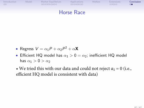
Horse Race
• Regress V = α1P + α2P2 + αX
• Efficient HQ model has α1 > 0 = α2; inefficient HQ modelhas α1 > 0 > α2
62 / 62
• We tried this with our data and could not reject α2 = 0 (i.e., efficient HQ model is consistent with data)