Organization of the course,
26
Fluctuations. Organization of the course, and facts Olivier Blanchard ∗ March 2005 ∗ 14.452. Spring 2005. Topic 1. 1
Transcript of Organization of the course,

Fluctuations. Organization of the course,
and facts
Olivier Blanchard∗
March 2005
∗ 14.452. Spring 2005. Topic 1.
1

1 Fluctuations. Overview
Intermediate textbooks have it right (it is essential that you read one)
In the short run •
The price level (that should move a lot under the flexible price assumption) adjusts slowly.So shocks to aggregate demand affect output rather than prices.Changes in nominal money translate into changes in real money.Monetary policy can control the interest rate.Current and expectations of interest rate and income affect aggregate
demand.Aggregate demand determines output and unemployment, which can
differ from the natural rate.IS-LM model, extended to incorporate expectations, captures mostof this.In the long run•
Prices/the price level adjust.Output, unemployment, the real interest rate all return to their natural rate. Money is neutral.Some shocks affect the deviations from natural rate, others the nat•
ural rate, others both.Things can go wrong:•
Can take very long to get to the long run. Great Depression. Japan
in the 1990s. And because of expectations of the future matter today, the medium/long
run affects the short run. Perverse effects of fiscal expansions. The hi tech boom.
The purpose of this course is to get to roughly the same place, but with
a deeper understanding of the mechanisms, of the imperfections. This is needed in particular if we want to think about welfare implications. In the
process, improve on the intermediate text models.
2
2 Organization
Facts. What are we trying to explain? •
The simplest model. A model with a C/S choice, uncertainty, and •
shocks. Natural starting point. Ramsey model (really Arrow Debreu).(Why Ramsey, not OLG? No good reason, except convenience.)Methodological contribution of Prescott here. Before, starting pointwould have been a more static version (for example, the book by
Patinkin, on “Money, interest, and prices”).Useful methodologically. C/S choice central to any model. But clearly
short of the mark. No employment movement (by assumption).Allowing for labor/leisure choice. Natural starting point to generate•
employment fluctuations.The RBC model (can still think of it as Arrow Debreu).Empirical problems at two margins. The existence and the nature
of technological shocks. The relevance of the labor/leisure choice to
fluctuations in employment in the labor market. But again, usefulbenchmark.Allowing for investment decisions. In benchmark RBCs, investment•
decision is trivial/degenerate; the interest rate is always equal to the
marginal product of capital. In fact, investment is a complex decision,and interest rates can/do diverge from marginal products. So, usefulto expand by allowing for costs of adjustment.Now: Both a saving decision and an investment decision. The sequence of intertemporal prices (term structure of interest rates) clears.(This is the mechanism that fails when nominal rigidities are present,below)A useful model to discuss two issues in particular. The dynamics ofthe current account (investment minus saving) in an open economy.The macro implications of mispricing of assets, such as bubbles, fads.Allowing for two goods. Much of our intuition in macro is based on•
3
a one–good model.But can be dangerous (some intuitions do not extend).And, in some contexts, open economy in particular, need to have two
goods. Domestic/foreign. Tradable/non tradable. The basic modelfor international macro.Clear evidence that movements in money affect output. (that the Fed•
is not irrelevant). So next step is to introduce money as a medium ofexchange.Forces us to think how a monetary economy looks like. The decentralization of exchange. The use of money in transactions.Natural question. Very different economy. What difference does itmake? The answer is: Not a lot, per se. Insights into fiscal policy,inflation. Not so much about fluctuations.Money as numeraire. Price setting. Monopolistic competition, with•
price setters. costs of adjusting prices.Deliver the basic implications, short run/medium run. Allow for welfare analysis. (Non trivial results, because start with imperfections)Look more closely at price setting/staggering. So, as to get close to•
a model we can use to think about policy.The current workhorse: The “New Keynesian Model”. Staggering ofprice/wage decisions. An IS curve based on intertemporal consumption choices, and a Taylor rule for monetary policy.Good enough? Probably not. The evidence on inflation and activity:More inflation inertia than implied by the model.Return to monetary policy.•
The shift to inflation targeting. Rules for central banks. How should
we design monetary policy in a world where expectations matter very
much? Inflation targeting, Taylor rules. The liquidity trap. What does it mean? What does it imply? Policy
implications.
4

Return to fiscal policy. •
Revisiting spending versus taxes as macro policy tools. Dynamic effects of fiscal policy. Can fiscal expansions lead to such
adverse expectational effects as to have adverse effects on output in
the short run? Automatic stabilizers. So, back to the stuff of textbooks. But hopefully, with more solid
foundations.
In short. Develop a model with:
Shocks. Which ones? Still unclear. •
Strong intertemporal mechanisms. Consumption smoothing. Invest•
ment.Imperfections. Monopolistic competition. Nominal rigidities. Which•
others?
Enough to start. But clearly many issues left aside, which affect the nature
and the effects of fluctuations. Credit market imperfections. Labor market imperfections.
14.453. Consumption, Investment decisions. More theory, more evi•
dence.14.454. Imperfections in goods, labor, credit, financial markets. Im•
plications for macro.
A word on the textbooks. Each useful in some dimension.
BF encyclopedic and simple, but a bit old. •
OR more consistent about the use of discrete time, and stronger on •
open economy.LS stronger on techniques.•
Woodford gives a good synthesis of New Keynesian models and ap•
plications.CW covers monetary issues, in an accessible way.•
5

3 Some Facts
3.1 Covariance stationarity
We can hope to characterize facts is only if there are some regularities. If things repeat themselves, in some well defined way.
This is what the expression “Business cycles” captures. If output high now, it is likely to still be high next quarter, next year, low two years from now.
For this, covariance stationarity is the relevant concept (for one variable, or a vector of variables).
Definition.
EYt = µ for all t
E(Yt − µ)(Yt−k − µ) = gk for all t
Then, we can hope to actually learn the moments, look at the stochastic
process, and do more.
Reasonable assumption?
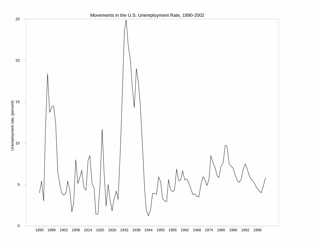
Sometimes not. Some episodes appear to be one of a kind. Unemploy•
ment during the Great Depression. (Graph). Hyperinflations. Transition in Eastern Europe. Maybe some deeper process which generates such episodes infrequently. But given the length of the series we have, this point is irrelevant. Sometimes yes. Post war US GDP. Not covariance stationarity as •
trends up (back to this in a minute). But a transformation of it seems to be. Use with care.
6
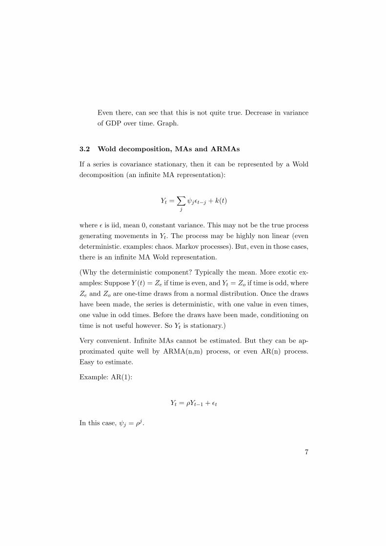
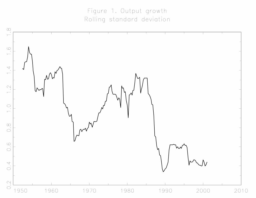
Even there, can see that this is not quite true. Decrease in variance
of GDP over time. Graph.
3.2 Wold decomposition, MAs and ARMAs
If a series is covariance stationary, then it can be represented by a Wold
decomposition (an infinite MA representation):
Yt = �
ψj �t−j + k(t) j
where � is iid, mean 0, constant variance. This may not be the true process generating movements in Yt. The process may be highly non linear (even
deterministic. examples: chaos. Markov processes). But, even in those cases, there is an infinite MA Wold representation.
(Why the deterministic component? Typically the mean. More exotic examples: Suppose Y (t) = Ze if time is even, and Yt = Zo if time is odd, where
Ze and Zo are one-time draws from a normal distribution. Once the draws have been made, the series is deterministic, with one value in even times, one value in odd times. Before the draws have been made, conditioning on
time is not useful however. So Yt is stationary.)
Very convenient. Infinite MAs cannot be estimated. But they can be approximated quite well by ARMA(n,m) process, or even AR(n) process. Easy to estimate.
Example: AR(1):
Yt = ρYt−1 + �t
In this case, ψj = ρj .
7
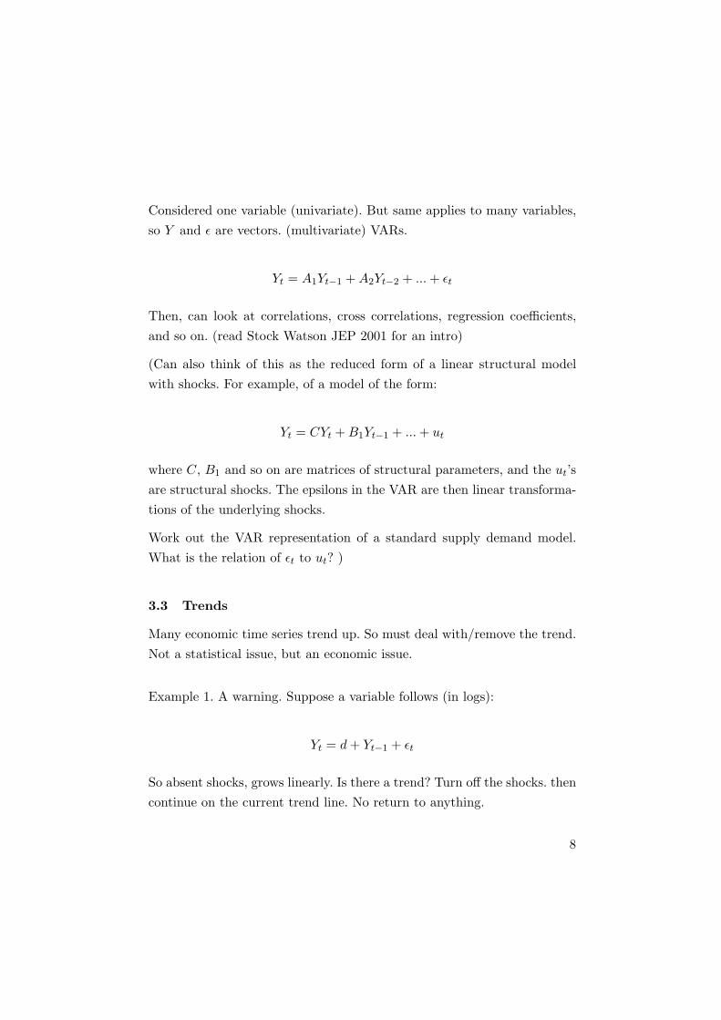
Considered one variable (univariate). But same applies to many variables, so Y and � are vectors. (multivariate) VARs.
Yt = A1Yt−1 + A2Yt−2 + ... + �t
Then, can look at correlations, cross correlations, regression coefficients, and so on. (read Stock Watson JEP 2001 for an intro)
(Can also think of this as the reduced form of a linear structural model with shocks. For example, of a model of the form:
Yt = CYt + B1Yt−1 + ... + ut
where C, B1 and so on are matrices of structural parameters, and the ut’s are structural shocks. The epsilons in the VAR are then linear transformations of the underlying shocks.
Work out the VAR representation of a standard supply demand model. What is the relation of �t to ut? )
3.3 Trends
Many economic time series trend up. So must deal with/remove the trend. Not a statistical issue, but an economic issue.
Example 1. A warning. Suppose a variable follows (in logs):
Yt = d + Yt−1 + �t
So absent shocks, grows linearly. Is there a trend? Turn off the shocks. then
continue on the current trend line. No return to anything.
8
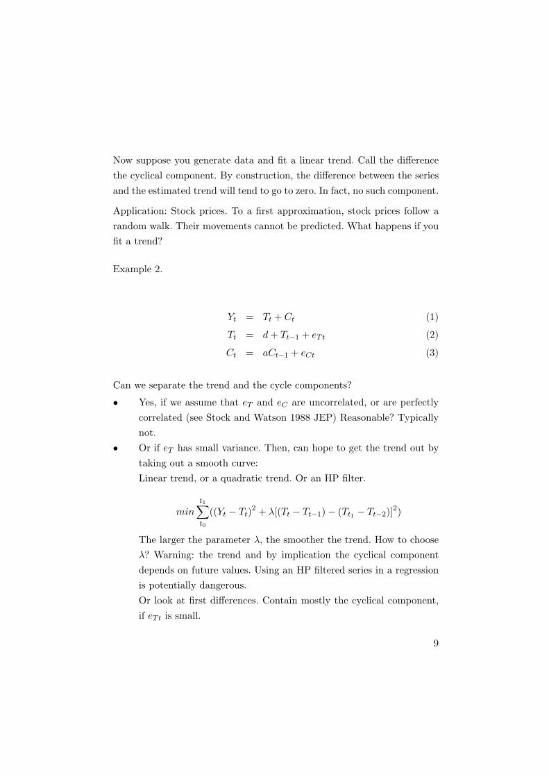
Now suppose you generate data and fit a linear trend. Call the difference
the cyclical component. By construction, the difference between the series and the estimated trend will tend to go to zero. In fact, no such component.
Application: Stock prices. To a first approximation, stock prices follow a
random walk. Their movements cannot be predicted. What happens if you
fit a trend?
Example 2.
Yt = Tt + Ct (1)
Tt = d + Tt−1 + eTt (2)
Ct = aCt−1 + eCt (3)
Can we separate the trend and the cycle components?
Yes, if we assume that eT and eC are uncorrelated, or are perfectly •
correlated (see Stock and Watson 1988 JEP) Reasonable? Typically
not.Or if eT has small variance. Then, can hope to get the trend out by•
taking out a smooth curve:Linear trend, or a quadratic trend. Or an HP filter.
t1
min �
((Yt − Tt)2 + λ[(Tt − Tt−1) − (Tt1 − Tt−2)]
2) t0
The larger the parameter λ, the smoother the trend. How to choose
λ? Warning: the trend and by implication the cyclical component depends on future values. Using an HP filtered series in a regression
is potentially dangerous. Or look at first differences. Contain mostly the cyclical component, if eTt is small.
9

How much of a difference? Results for GDP. Graph. •
The frequency domain. Instead of the infinite MA representation, can •
characterize behavior by the spectrum, giving the importance of the
components at different frequencies. Then, can take out the very low frequencies, perhaps the very high
ones. Keep the part of the spectrum corresponding to 6 quarters to 8
years. This is the Stock Watson approach (Handbook 19990. Graph.
3.4 Co-movements of output with components.
Stock Watson looks at the correlation between cyclical components of output and other variables.
ρ(Xct, Yct+k ) k = −6, ..., 0, ..., +6
(in quarters)
If ρ is positive and highest for k < 0, then X is procyclical and lags.
If ρ is positive and highest for k > 0, then X is procyclical and leads.
Does not give us a sense of the amplitudes. Covariances rather than correlations would.
Results (Table 2)
Output, consumption. high and positive. col 9. •
Output, investment high and positive. col 14. •
Surprising? More than you might think. You might have thought that fluctuations came from changes in discount rate (people really
liking the present, so consuming more, may be working less, then
investment would go down.) Output and inventory investment high and positive. col 18. •
10

Should you be surprised by this? Yes, if Keynesian. High demand
should be smoothed by firms, leading to negative investment. Change
in the 1990s: the correlation has become less positive. Little correlation with exports. col 19. In the US, fluctuations do not •
look export driven. (Look at the same correlation for a small open
economy, say Belgium).Little correlation with government spending. cols 22 to 24. In the US•
(and in most other countries) fiscal policy is not a major source offluctuations.Looking across sectors. cols 1 to 8. High correlation for all, except•
mining. (Similar results in Christiano et al) A clear indication of how
far we are from the old cycles.
3.5 Comovements with employment
correlation with employment high and positive. col 25. lag. suggests •
output then bodies.Should also be seen as a surprise: If booms are good times, why take
less leisure? Or if value utility more now, then why not take both
more consumption and more leisure?
Coincident with hours. col 27. suggests adjustment at that margin.•
First, firms adjust with overtime, then over time, through hiring. High and positive with total factor productivity (Solow residual) and •
average labor productivity. cols 32 and 33. Leads.
3.6 Comovements with prices and wages
One central intra-temporal price: the real wage. One central inter-temporal price: the real interest rate.
Not much cyclical movement in either.
11

Cyclical component of the wage? (think about detrending) •
Real wage (definition of the deflator is not given). col 44. probably
real product wage. Slightly pro-cyclical, but not much. A-cyclical is a good characterization. Clearly inconsistent with only movements along a labor demand
curve, or labor supply curve. (Old Keynes/Tarshis discussion) consistent with shifts in labor demand, or a mix. or with a model with
further deviations from standard labor market equilibrium. Correlation with interest rates. •
Nominal: col 47 to 49. strongly procyclical and lags output. High in
booms. Real: col 50. mildly countercyclical: low in booms. Leads output a
bit. This suggests a story in which low interest rates lead to high
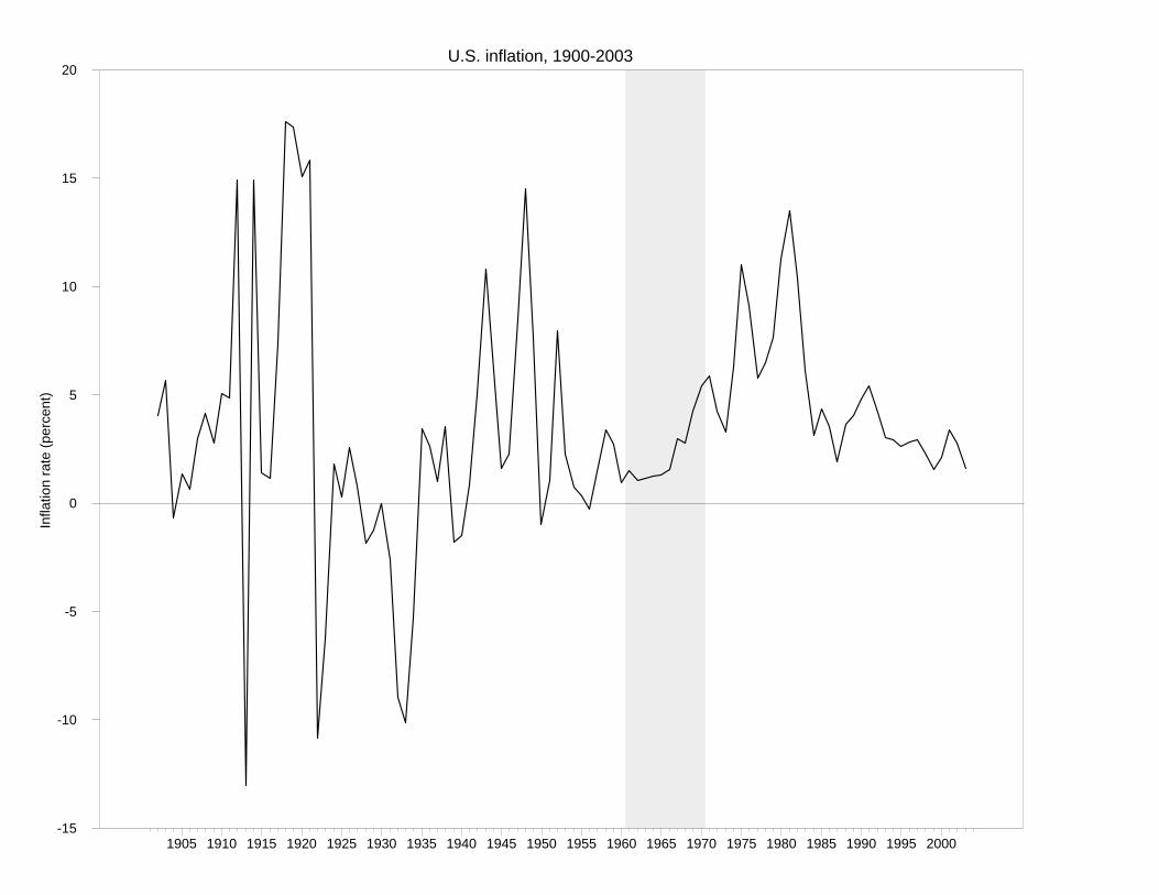
demand and high output, but then leads to higher nominal rates. Now look at correlation with inflation (GDP deflator or CPI). cols •
39, 41. strong correlation, max at lag 4.This is the Phillips curve relation. More standard scatter diagram.High GDP, low unemployment, leads to higher inflation with a lag.
3.7 Co movements with money
.
Long held belief that money has major effects on output. Friedman and
Schwartz on Great Depression. The Volcker recession of 1980-82. Surely, markets believe that the Fed can affect output. Federal funds rate and
output.
Correlations high. Both nominal and real. Columns 54, 56. But what •
does this prove?
Need more convincing identification. Will just present the results of•
the study by Christiano et al. (based on a VAR)
12
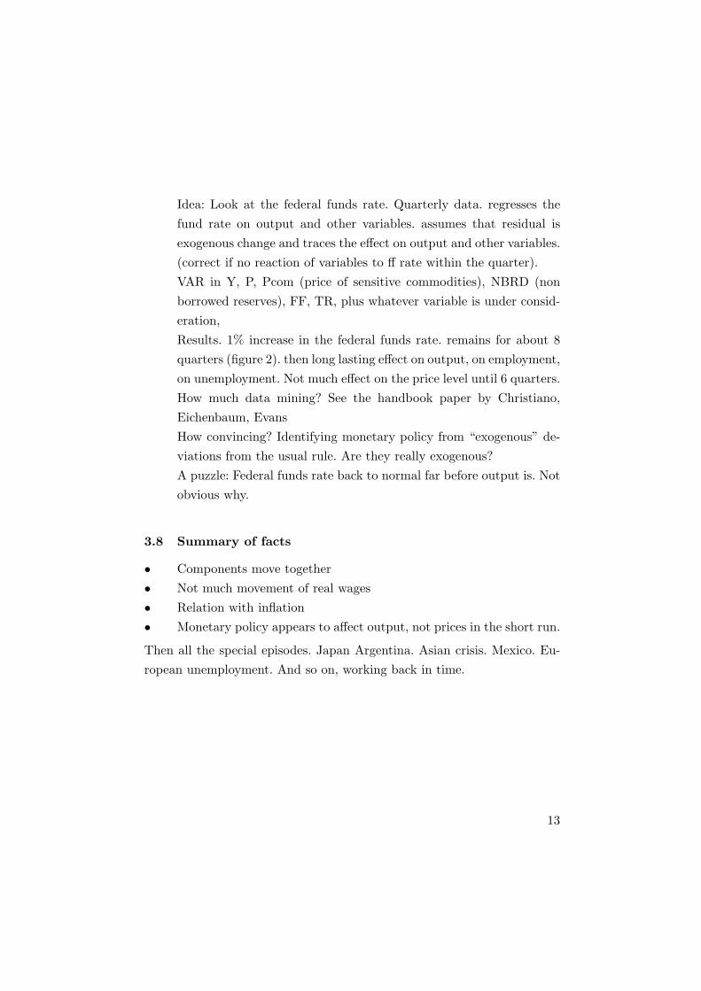
Idea: Look at the federal funds rate. Quarterly data. regresses the
fund rate on output and other variables. assumes that residual is exogenous change and traces the effect on output and other variables. (correct if no reaction of variables to ff rate within the quarter). VAR in Y, P, Pcom (price of sensitive commodities), NBRD (non
borrowed reserves), FF, TR, plus whatever variable is under consideration, Results. 1% increase in the federal funds rate. remains for about 8
quarters (figure 2). then long lasting effect on output, on employment, on unemployment. Not much effect on the price level until 6 quarters. How much data mining? See the handbook paper by Christiano, Eichenbaum, Evans How convincing? Identifying monetary policy from “exogenous” deviations from the usual rule. Are they really exogenous?
A puzzle: Federal funds rate back to normal far before output is. Not obvious why.
3.8 Summary of facts
Components move together •
Not much movement of real wages •
Relation with inflation •
Monetary policy appears to affect output, not prices in the short run. •
Then all the special episodes. Japan Argentina. Asian crisis. Mexico. European unemployment. And so on, working back in time.
13
Une
mpl
oym
ent r
ate,
(per
cent
) Movements in the U.S. Unemployment Rate, 1890-2002
25
20
15
10
5
0 1890 1896 1902 1908 1914 1920 1926 1932 1938 1944 1950 1956 1962 1968 1974 1980 1986 1992 1998
Infla
tion
rate
(per
cent
) U.S. inflation, 1900-2003
20
15
10
5
0
-5
-10
-15 1905 1910 1915 1920 1925 1930 1935 1940 1945 1950 1955 1960 1965 1970 1975 1980 1985 1990 1995 2000

log Y and linear time trend log Y and hp filter (1600)9.25
LY FIT1
9.25
9.00 9.00
8.75 8.75
8.50 8.50
8.25 8.25
8.00 8.00
7.75 7.75
7.50 7.50
7.25 7.251948 1951 1954 1957 1960 1963 1966 1969 1972 1975 1978 1981 1984 1987 1990 1993 1996 1999 1948 1951 1954 1957 1960 1963 1966 1969 1972 1975 1978 1981 1984 1987 1990 1993 1996 1999
LY HPFIT1
log Y and quadratic trend log Y and hpfilter(16)9.25
LY FIT2
9.25
9.00 9.00
8.75 8.75
8.50 8.50
8.25 8.25
8.00 8.00
7.75 7.75
7.50 7.50
7.25 7.251948 1951 1954 1957 1960 1963 1966 1969 1972 1975 1978 1981 1984 1987 1990 1993 1996 1999 1948 1951 1954 1957 1960 1963 1966 1969 1972 1975 1978 1981 1984 1987 1990 1993 1996 1999
LY HPFIT2

log Y detrended
0.075
0.050
0.025
-0.000
-0.025
-0.050
-0.075
-0.100
0.100 RES1 RES2 HPRES1 HPRES2
1948 1951 1954 1957 1960 1963 1966 1969 1972 1975 1978 1981 1984 1987 1990 1993 1996 1999

Impulse responses, linear and quadratic trend0.014
0.012
0.010
0.008
0.006
0.004
0.002
0.000
RESPLINEAR RESPQUAD
5 10 15 20 25 30 Quarters
Figures 2.5-2.7 removed for copyright reasons.
Stock, J., and M. Watson. "Business Cycle Fluctuations in U.S. Macroeconomic Time Series." Chapter 1 in Handbook of Macroeconomics. Vol 1A. Edited by J. Taylor and M. Woodford. Amsterdam; New York: North Holland, 1999. ISBN: 0444501568. (PDF - 2.2 MB)

Table 2 removed for copyright reasons.
Stock, J., and M. Watson. "Business Cycle Fluctuations in U.S. Macroeconomic Time Series." Chapter 1 in Handbook of Macroeconomics. Vol 1A. Edited by J. Taylor and M. Woodford. Amsterdam; New York: North Holland, 1999. ISBN: 0444501568. (PDF - 2.2 MB)

Table 2 removed for copyright reasons.
Stock, J., and M. Watson. "Business Cycle Fluctuations in U.S. Macroeconomic Time Series." Chapter 1 in Handbook of Macroeconomics. Vol 1A. Edited by J. Taylor and M. Woodford. Amsterdam; New York: North Holland, 1999. ISBN: 0444501568. (PDF - 2.2 MB)

Table 2 removed for copyright reasons.
Stock, J., and M. Watson. "Business Cycle Fluctuations in U.S. Macroeconomic Time Series." Chapter 1 in Handbook of Macroeconomics. Vol 1A. Edited by J. Taylor and M. Woodford. Amsterdam; New York: North Holland, 1999. ISBN: 0444501568. (PDF - 2.2 MB)
Figure 2.3 removed for copyright reasons.
Christiano, L., M. Eichenbaum, and C. Evans. "Monetary Policy Shocks: What have We Learned and to what End?" Handbook of Macroeconomics. Edited by J. Taylor and M. Woodford. vol. 1A. Amsterdam; New York: North Holland, 1999, pp. 65-148. ISBN: 0444501568. (PDF - 1.9 MB)

Figure 2.4 removed for copyright reasons.
Christiano, L., M. Eichenbaum, and C. Evans. "Monetary Policy Shocks: What have We Learned and to what End?" Handbook of Macroeconomics. Edited by J. Taylor and M. Woodford. vol. 1A. Amsterdam; New York: North Holland, 1999, pp. 65-148. ISBN: 0444501568. (PDF - 1.9 MB)
Figure 2 removed for copyright reasons.
Christiano, L., M. Eichenbaum, and C. Evans. "Monetary Policy Shocks: What have We Learned and to what End?" Handbook of Macroeconomics. Edited by J. Taylor and M. Woodford. vol. 1A. Amsterdam; New York: North Holland, 1999, pp. 65-148. ISBN: 0444501568. (PDF - 1.9 MB)