ORBITS ASYMPTOTIC TO THE STRAIGHT LINE EQUILIBRIUM POINTS IN THE PROBLEM OF THREE FINITE BODIES ~).

By D a n i e I 8 u c h a n a n (Vancouver, Canada).

Adunanza del 25 aprile 192o.

Introduction.

It was shown by LAGRANGE in a prize memoir ~) in 1772, that it is possible to

start three finite bodies, subject to the Newtonian law of attraction, in such a way

that they will describe similar ellipses in the same time. There are two configurations

which the three bodies will maintain in describing these orbits, viz., they are either

collinear or they lie at the vertices of an equilateral triangle. The positions in these

configurations are called respectively the straight line and the equilateral triangle equi- librium points in the problem of three finite bodies.

The purpose of the present paper is to show that there is a class of orbits in the neighborhood of the straight line configuration 3) which approaches the straight

line equilibrium points as the time approaches infinity. Such orbits are called asymp-

totic orbits 4).

The particular Lagrangian orbits, to which the orbits constructed in this pape r

2) Presented to the American Mathematical Society, Dec. 28, I918. ~) Ch. LAORANOE, Oeuvres compZ~tes, (Paris, Gauthier-Villars), vol. V!, pp. :~9-~4; P. TIs-

S~RAND, Traitg de Micanique celeste, t. I (Paris, Gauthier-Villars, ~889), Chap. VIII; F. R. MouT.TON, Introduction to Celestial Mechanics (New York, Mac Millan, 1914), pp. 3o9-318.

3) The orbits whi'ch are asymptotic to the equilateral triangle configurations are at present under consideration and will be discussed in a subsequent paper.

4) H. POXI,/CAR~I Les M3thodes nouveUes de la M~canique celeste, t. I (Paris, Gauthier-Villars, I892), Chap. VII.

6~BITS ASYMI~TOTiC TO THE STRAICHT LI~E EQUILIBRIUM POINTS, ET~. ~3~

are asymptotic, are those described when the three bodies are so projected that they

will remain collinear and move in complanar circles. The paper concludes with a numerical example in which the three masses are

assigned particular values and are givon certain initial displacements from the periodic

orbits. Classes of asymptotic orbits in the problem of three bodies have already been

obtained, but, unlike the present paper, they all deal with the case in which one of the bodies is infinitesimal. Warren obtained two dimensional orbits which are asymp- totic to the straight line equilibrium points, and the following asymptotic orbits s)

were obtained by the author of the present paper. I. Two- and three- dimensional orbits 6) which are asymptotic to MouLvo~q's

c~ Oscillating Satellites 7 ) , of class B and class A respectively. 2. Two-dimensional orbits s) which approach the equilateral triangle equilibrium

points. 3. Two- and three- dimensional orbits which are asymptotic respectively to the

two- and three-dimensional periodic oscillations about the equilateral triangle equilibrium points that were obtained by Buck: 9).

4. Three-dimensional orbits ,o) which are asymptotic to the isosceles-triangle solu-

tions *~).

2.

The Differential Equations.

Let the masses of the three finite bodies be denoted by m,, m 2, and m 3. Let a , system of rectangular axes be chosen having the origin at the centre of gravity of

s) L. A. H. WA~E~, A class of Asymptotic Orbits in the Problem of Tloree Bodies [American Journal of Mathematics, vol. XXXVIII (i916), pp. 22:-248].

6) D. BUCHANAn, Asymptotic Satelites near the Straight-Line Equilibrium Points in the Problem of Three Bodies [American Journal of Mathematics, vol. XL! (19:9) , pp. 79-iio].

7) F. R. MOVLTON, Periodic Orbits (Washington, Carnegie Institution, I92o), Chap. V. s) D. BUCHANAN, Asymptotic Satellites near Equilateral Triangle Equilibrium Points in the Problem

of Three Bodies [Transactions of the Cambridge Philosophical Society, vol. XXII, No. XV (i919) , pp. 309-340].

9) Chap. IX of MOULTON'S Periodic Orbits, loc. 7). to) D. BUCHANAN, Orbits Asymptotic to an Isosceles.7u Solution of the Problem of Three

Bodies [Proceedings of the London Mathematical Society, Series II, vol. XVII, Part x, pp. 54-74]. xx) D. BtSCHANAN, Chap. X of MOULTON'S Periodic Orbits, 1. c. 7).

334 D A N I E L B U C H A N A N ' .

the three bodies and, since they are assumed to be complanar~ their plane of mot ion

will be chosen as the ~'t,-plane. Let the coordinates of rn~ be (~i, "~), (i = I, 2, 3). Then the differential equations of motion are

(i)

d'~, I 8 U dt~ - - m l O~i '

d2~#, i I 8 U

dt ~ - - r n i c3"~ i '

(i : I, 2, 3),

k21 ml m2 m2 m3 m3 m t l u = + +

r,i = [(~- - - ~i)' -[- (~, - - ~i) ~]'/~' (i, ] = x, 2, 3; i 761),

where k ~ is a factor of proportionality. Let the motion of the system be referred to a set of rectangular axes rotating about the I-axes with the uniform angular velocity n. The required transformation is

1~r - - x~ cos n t - - y; sin n t, (2) "~, = x, sin nt + Yi COS at,

( i = I, 2, 3),

where (x; , y~) are the coordinates of m i with respect to the rotating axes. Then the differential equations ( I ) become,

(3)

d~xr dy i I 0 U d t ~ ~ 2 n d i - - - n2xi m; O x i = o,

d2y~ dx~ __ n2 I 0 U

( i = x, 2, 3),

where U is the same as in ( I ) , but

r,i = [ (x , - x j ) ' + (y, - y ) ' ] ' / , , (r j = I, =, 3; r S).

The Straight Line Equilibrium Polnt~,

If the bodies are projected so that they will move in circles about the origin with the uniform angular velocity n, then their coordinates with respect to the rota- ting axes are constants. Hence the first and second derivatives in equations (3) are

ORBITS A~YMPTOTIC TO THE STRAIGHT LINE EQUILIBRIUM PO I N T S , ETC. ~ 5

zero and these ec

(4)

uations reduce to

n2x, + k2m~ -

- - n2x~ .3 7 k ~ m , - -

X - - X 2 Xf - - X 3 + k 2 m3 . . . . . . = o,

r i 2 r 3 x3

x a - - x~ .~2 x a ~ x 3

3 + /g ~F/'3 r3 ~ O, r12 23

X - - X t X - - X 2 - - n~x3 + k2rn 3 2 r3 -1 V k m~ 3 r 3 = o,

z3 23

- n~y, + k~m2 y~ - - Y: d 1- k: Y, - - Y3 r~ 2 'm'3 3 ~ O,

r t 3

,2 Y ~ - - Y , k ~ Y~--Y3 - - n ~ y ~ + R m, ~ + m~ 3 - - o ,

r~2 r2 3

- - Y____~' k~ 23 ~ )'2 - - n~ Y3 + k2m,y3 r 3 21- m, r3 - - o.

13 23

Conversely, if the masses and initial projections are such that equations (4) are

satisfied, then the bodies will move in circles about the origin with the uniform

angular velocity n. Hence equations (4) are the necessary and sufficient conditions for

the existence of circular orbits.

Obviously the last three equations of (4) are satisfied by y, - - Y2 - - Y3 -- ' o. On making use of the centre of gravity equation

(s) ,,~ x + m2 x + m 3 x 3 = o, it is found that the first equation of (4) is a consequence of the second and third

equations. Hence the first equation of (4) can be replaced by equation (5). If the units of distance and of time are chosen so that r,~ and k 2 are both unity, then the three equations which define the straight line equilibrium points are

l ~ m ' x ' + m ~ x ~ + m 3 x 3 - - ~

X - - X 3 (6) n2., - , + m (x - x 3 + m 3 r3 _ o ,

. 1 3

X 2 - - X 3 n 2x + m ( x ~ - x l ) + m ,3 - o .

23

If the bodies lie in the order m , m2, m 3, from the negative to the positive end

of the x-axis, then x 3 > x~ > x , and r2 = x 2 - - x - - I. Equations (6) may there- fore be simplified to

(7)

I r n x . - ~ r n ( i .Ayx).-~-rn3x 3 - - o ,

m~_ ,n~ + (,,. _ x ? + ~ x = o,

- - m + ( x - x - i ? + ~ ( I + x ) = o .

336 D A N I E L B U C H A N A N .

Now let X 3 - - X 2 ~ A , ,,, + ,,= + ,,~ = M.

Then from the first equation of (7) it follows that

~ + m (~ + .4) ( 8 ) x , = - U

When n' and x 3 are eliminated from (7), and (8) is substituted in the result, we obtain

(9) ? (,,,~ + 3 m) ,4~-- (2 m, + 3 m) .~ - - (m~ + ~ ) = o,

which is LAGRASGE'S quintic equation. Since there is but one change of sign in the coefficients, this equation has but one real positive root. As only a positive value of A is valid for the chosen order of the masses, there is therefore but one solution of (9) which determines the straight line equilibrium points. By cyclically permuting the order of the three bodies, two more distinct straight line solutions will be obtained =~).

~4 .

The Equation of Variation.

In order to determine orbits which approach the equilibrium points asymptotically, we displace the bodies slightly from their equilibrium points and then so determine the initial conditions that the bodies will approach the equilibrium points as the time approaches infinity.

Let the coordinates of the equilibrium points be ( x , o), (32, o), and @3' o) for m,, m 2, and m 3 respectively. For the order of the masses chosen in the preceding

section, x 3 D x2 ~ x . Since the centre of gravity equations

0o) m,x,-Jr-m2x~ + m3x3=o, m,y,-]-m,y,-]-m3y3=o

are always satisfied, they may be used to eliminate two of the variables, x s and y~ let us suppose, from the differential equations of motion.

z~) A determination of the straight line eqailibrium points to which the preceding is somewhat

similar may be found in any treatise on Celestial Mechanics, but see MOULTON'S b,troduction to Cele-

stial Mechanics~ 1. c. a), pp. 3o9.312.

ORBITS ASYMPTOTIC TO THE STRAIGHT LINE EQUILIBRIUM POINTS, ETC. 337

Now let

( , 0

where u ~ . . . , v 2

bodies m and m~

that

( ,2)

X I ~ X I + U 1 ~ X 2 : X 2 + Z# 2

y , : o + v , y ~ : o + v ,

denote the x- and y- components of the displacements of the

from the equilibrium points. Then from ( , o ) and (II) it follows

When

equations for the motion of m, and m become

I [m, (x, 71- u ) Jl- m, (x, -~- u,)], X3 - - - 7/~

3

I Y3 - - - - ~ [m v, .+ m2"/)2] .

m 3

the substitutions ( i i ) and ( I 2 ) are made in equations (3), the differential

i ( D ~ 2 r - a ,) u, -3 I- a, u ~ - - 2 n D v , --- U~" 2r - U"~ + . . . 3

2nDu , + ( D ~ + / , ) v i + b v - - - V f + V ( ' ) + . . . c , ~ + ~ ' k J J

I c ~ u . + ( D ~ + c , ) u ~ + - - 2 n D v ~ = U ( ~ ) - F U ( ~ ) - F . . .

2nhu~ -F d,v, + (D ~ -{- d,)v~ -- V(~)-[ - V(~)-F. . .

d where D denotes the operator -~- and,

2(m, JI- m ) a, = - - n ~ - - 2 m~ (I + ~)~

m -F m 3 b, - - - - n~ + m , -F (i + - ~ ) , ,

2 ( m J i - m 3 ) C l ~ - - H2--27t]~l A 3 ,

d,=--"~+m,+ m~+m

[ ' ] a , = 2 m ~ , ( , + v / ) ' '

b = - - m , ~ (~+~4)i '

C 2 = 2 m x I - -

d 2 - - - - m , E ' - - ~ f ] ,

I 2 I

(~F)~ L + 4 ( m' § m,)., +m+.+t +m)v

3 m m v m v m m )u m u V(2'~----3m2(v,--v2)(u,--u2)--m3(I_FA)4{( iJF 3),~L 2 2t{( ,+ 3 iJF 2 ~I,

U(2>__ 3m ' ( u _ u ), - i ~ , E 2-(V'--V]) ] -1-- m-~t m' u ' Jl-(m2 JF m3)u2/2

2,] j+/.,,v, + ( m2+,,Ov./',

[r(,) m v v u u 3 m y m m v m u m m u ~2 =3 ,( , -D ( , - Y - m - ~ l , ,+( ~+ 3)~} / , ,-t( ~+ )~I. J~tnd. Cim. Matem, Palerrno~ t, XLV ( i 9 2 x ) . - Sttmpato il 7 ottobrr 1~11, 4~

338 D A N I E L B U C H A N A N .

The remaining U(. il V I~/ (i := [, 2; j = 3, 4, �9 co), are polynomials of de- I ' J ' " "

gree j in u , u~, v , and %. If we neglect the right members in ( I3) we obtain the equations of variation,

(,s)

I (D ~ + a ) u _3r a u - - 2 n D v , = o,

2 n D u + (D ~ + bx)v ' + b % = o,

c u -~- (D ~ + c,)u2 ~ 2 n D v ~--- o,

2 n h u, -3 V d , v , -3 c- ( D ~' -it- d ) v, - - o.

S o l u t i o n s o f the E q u a t i o n s o f V a r i a t i o n .

T h e equations of variation are a set of simultaneous

coefficients. Following the well-known method of solving such to zero the determinant formed by the coefficients of u,, u, ,

Thus

0 6 ) ~ - -

equations having constant equations, we equate

v,, and v~ in (I5).

D* + a a 2 - - 2 n D o

2 n D o D 2 + b , b

c~ D' + c, o - - 2 n D

o 2 n D d~ D*-[--d

Since it is found that b d, = b2d, then

~ - 0 .

(17) D 2 V .2 X2. i ' A 2 ' o r 3

Since the determinant, apart from the factor D 2, is a cubic in D*, one of these roots in always real and the other two are either real or conjugate complex. The roots of

(I6) are therefore

D = o, o, ___+ X, + X,, + X,

Obviously, the determinant A vanishes for D ~ - - o. Let the remaining roots be

A==_--D2[D6+ D4(a -J-b + c -{-d, +8n2)-i-D2{(a,-J-b + 4n2)(c,-{-d, -[-4 n2)

2vc, d,(a,-dvb, + 4n~)2f-4n~(a~d~dvb~ c~)--b~ d~(a, + c , ) - -a~ c~(b,'dvd,)].

ORBITS AS?MPTOTIC TO TI'~E sTRAIGHT LiNE EO_IJILIBRIUM POINTs, ETC. J~9

and consequently the solutions of (I5) are

08)

b2 ~ O) - e~xt = - - ~ (~3 ~4 e-~''') V, ~ ( , + ~, t) + - -

+ ~7' (~'~ ?~' - ~'~ ~-~') + ~'," (~'~ ?~' - ~ ~-~'),

2 n (a, b + b= c3 L (~ + %e-x") u, --" b , (a , c , - - a=c=) % -It" ") - eL'

v , = ~ , + ~ t + ~';'(~ ? ' , ' - -~e -~,') + ~ ( ~ - ~e-~, ') + - ~,,e-~,'),

}.) __ X { oy ),=,(a, -[- b --[- 4 n ' ) - [ - a b Jr- b,c= - - ),~ (a= -~- b=) -]- a ~ b, + b 2 c , '

2 n X ' 2V a --~ a~r~ a,

~(1) I 3 - - 2 n ),, [0'~ "{- C,)~{~/' -1 t- Q],

where %, %, . . . , % are the constants of integration.

(i----- i, 2, 3),

T h e Asymptotic Solutions.

We desire the solutions of 0 3 ) which are asymptotic in the sense of Pot~- CAR~ ,a), that is, each term of the solutions must have the form eZ 'P( t ) , where ). is a

number whose real part is different from zero, and P ( t ) is a constant or a periodic function of t. Such asymptotic solutions approach zero as t approaches + oo or - -oo

according as the real part of ), is negative or positive, respectively.

We shall consider in ~ 7 the solutions which approach zero as t approaches

+ oo and then show in ~ 8 that the solutions which approach zero as t approaches

oo can be obtained directly from the former solutions. The f o rma l construction of

the solutions will first be made and then their convergence will be considered in w 9.

~a) 1. r 4), p. 34o.

~4 0 DANIEL BuC HA.~AI~.

Various cases will arise in the construction of the solutions according to the forms of the roots ;~, X~, and ;~ in (I7) . They are:

Case I . - One positive root and two negative roots. Case I L - T w o positive or two conjugate complex roots and one negative root. Case I I L - Three positive roots, or one positive root and two conjugate complex

roots. CASE I V . - - T h r e e negative roots.

In order to construct asymptotic solutions, it is necessary that at least one of the t~ shall have a real part which is different from zero. Under the conditions of Case IV, all the ),~ are purely imaginary and in this case it. is impossible to construct the asymptotic solutions according to tlae method developed in this paper if, indeed, Such solutions exist.

57.

Construction of the Asymptotic Solutions.

We shall consider in this section solutions of 0 3 ) which approach zero as t ap- proaches q--oo. Let

( 1 9 ) U t - - - ~1* , U2 ~ ~ # 2 ~ V = ~ V ~ , V a - - - ~ V 2 ,

where ~ is an arbitrary parameter which, we shall see later, represents the scale fac- tor of the asymptotic orbits. When equations 0 9 ) are substituted in 0 3 ) and the fac- tor ~ is divided out, we obtain

'(D*-~ -- a ) u + a~u~ - - 2 n Dv, = ~ UI] ) --]-- ~ U 3-(') -+- . . . ,

2 .2 T1 ( , ) 2nD-u, + ( D ~ + b , ) v , + b~v~ =~p(~)'~-~ "3 + ' " ' (2o)

+ (D" + - - 2 = + + . . . , 3

2 n D u ~ + d v -[-(D ~ - { -d , )v ,=Sp~' )+8 '~ i ' )+ . . . 3

where U'!;) and F it) (i----- x, 2 ; j = 2 , 3, , oo), are the same as UIY ) and vtl) I J ' " ' " ] " J '

respectively, in ( I 4 ) i f the variables u , . . , % in 0 4 ) are replaced by u , , . . . , % , respectively.

We propose to obtain solutions of (20) as power series in = and accordingly we put

1~! "- ~ UI i ~t 9 lr --'- ~ U2i , . o

Ok~ITg AsYMPToTid TO THE STRMGHT LII'~E EQUILIBRIUM POINTS, ETd }4f

Let (2 i ) be substituted in (20) and let the resulting equations be denoted by (20'). Then, on equating the coefficients of the various powers of ~ in (20'), we obtain sets of differential equations which will determine the various u , , . . . , v~ in (21) in terms of initial conditions to be chosen later [see equations (22)].

Obviously, the complementary functions of the differential equations obtained by equating the coefficients of the same powers of ~ in (2o') are the same as the solutions of the equations of variation, viz., equations (I8). In order to obtain the asymptotic solutions, it is necessary to reject at each step of the integration all the terms of the complementary functions which do not satisfy POINCAR~'s definition of asymptotic solu- tions. It is therefore necessary at this stage of the construction to treat separately the different cases mentioned in ~ 6.

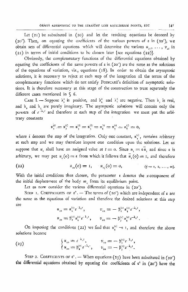
CASE I . - -Suppose ?,~ is positive, and 2: and ~-' , ~ ,3 are negative. Then ~, is real, and ),~ and ~'3 are purely imaginary. The asymptotic solutions will contain only the powers of e -z'' and therefore at each step of the integration we must put the arbi- trary constants

2 3 5 ~6 7

where i denotes the step of the integration. Only one constant, ~ , remains arbitrary at each step and we may therefore impose one condition upon the solutions. Let us

suppose that u shall have an assigned value at t = o. Since u = ~ u and since ~ is

arbitrary, we may put u ( o ) - - ~ from which it follows that u ( o ) = I, and therefore

(22) U,o(O) = . j ( o ) = o, <j= i , . . . . . .

With the initial conditions thus chosen, the parameter ~ denotes the x-component of the initial displacement of the body m from its equilibrium point.

Let us now consider the various differential equations in (20'). STEP 1. COEFFICIENTS OF : . - - The terms of (2o') which are independent of ~ are

the same as the equations of variation and therefore the desired solutions at this step are

U __. ~(~) g--)qt (~) - ( 0 g - k d 1o 4 } r I O ---- ~ ~ I ~ 4 '

U2o = --2 ~( ' ) ~(4 ') g - ) ' t t ' ~J20 = - - "3~(I)~(4 t) g - -~ i t .

On imposing the conditions (22) we find that x ") = I, and therefore the above 4

solutions become

r I O ~ ~ 9 ( 2 3 ) ~ UlO = g--~'lt ~j{l I } e--~*l ]

STEP 2. COEFFICIESTS OF ~'. - - When equations (23) have been substituted in (2o') the differential equations obtained by equating the coefficients of r in (2o') have the

~42 D A N I E L BUCHANAN ~.

form

(D z - ~ - a ) u + a,u=, - - 2nDv , = U --~-A,,e -=z,',

2nDu --[-(D ~ + b , ) v + b % , - - V , , ~ B , e -~z''

(24) i c,u + ( D z - { -c )u - -2nDv~, = U ~ A , , e -zz,~, 2nDu2i -3 t- d2v -a t- (D ~ + d,)v,, = V ~ B,,e -'z,',

where . 4 , . . . , B~, are constants. The complementary functions of these equations are the same as (18) but only the terms in e -x'' are to be retained. The particular integrals are

( z s ) i A( 0

A<, '] e_zz,t e-Z;.d ~, - zZ U e-zzv u , - a ( - 2 x , ) ------ , v , , - a ( - - ,

AO) a(l l e--2zlt e_2Z, , 41 e_2Zl] ,1 _~tZl ,

U2I - - A ( - - 2 ) , , - - ) ~ - 0~21 ' '/')2, - - 3l(__ 2),i ) ~ ~2 'e "

The symbols employed in (25) are defined as follows: A(-- 2)`~) denotes the determinant • equation (I6)7 when D is replaced by - - 2),,; AI. ') (j - - 1, 2, 3, 4), denotes the preceding determinant ~ ( - - 2) . ) when the elements j , ' in the fih column, reading from top to bottom, are replaced by . 4 , B , .,'/~,, and B~, respectively.

These particular integrals (25) are found to have the same form as the right members of (24) and therefore ~ , %,, ~. and ~, are constants. The solutions at this�9 step which have the proper exponentials are

r 0t(2)e--Xtt + ~ I | U 4

V - ' - - - - B/00~(Z)e-~'V .71- B e -~xd

From the initial conditions above solutions become

2 2, '

- ( ~ - and therefore the (22) it follows that ~4 - - - x,,

( 2 6 )

x ~ ,, ~(2) -2Zp' - - t e-2kd - - 0~(l)e-Zlt + ~i e U l - - v. e-X't "3V ~ll

u,, = - - ~l') , , e-Z,, ._~ ~2, e-'Zd ------ "12'~ e-z't -~- ~'~)e-ZZ'i,

V~, -- ~(')o~ e -z,t -~- ~ e -~)',t ~_ ~0)e-Zd _it_ fa(~) -zZ,t .~ ,, 2t iaa, e .

The remaining steps of the integration are similar to the preceding step, and an induction to the general term will show that the integration can be carried on inde-

�9 finitely. Let us suppose that ua , u~k , v,~, and v,~, (k = o , . . . , n - I), have been

ORBITS ASYMPTOTIC TO THE STRAIGHT LINE EQUILIBRIUM POINTS, ETC.

determined and that

~43

Ui~ ̀ --- L ~U) e , ( i = I, 2),

(27) J=' ~,., = ~ G'~-i~",

where the various ot(Jilk and ~q)ik are known constants. We desire to show that ul. and v;. have the same form as (27) if k - - n.

STEP n q - I . COEFFmmNTS OF a " . ~ T h e differential equations at the step ( n + 0 have the same left members as in (24) if the second subscript on the variables in (24) is replaced by n. If the corresponding right members are denoted by U,, , V . , U , and V, , , then it is found that

U i " = E A(JJ ' ( i = I, ~ , (28) ~=2

n + l

C. = Y Z~i' e-J~, ' in j = 2

where d/j) and B (i) +. +, are known constants. The Complementary functions of the diffe- rential equations at this step are

~l)) - - - 0~(; 0 g-~'l t ' /'/'an ----- -zBCi) ~(n)4 e-;Llt )

- z 4 ) V2 n _._ ~ ~ ( 1 ) ~ ~)g- -~ j t n 3 )

where ~l,,) is an arbitrary constant. The particular integrals are 4

(29)

I -*-, Aft) ,,-~, .

j=2 ,,§ A(J )

u2,,-- j ~ a ( ~ e-j;''' =- ~- ~(Jl e-12. ' j=a

Iv'"= ~ . _ _ . e-;~"'-~ Y~ 'j'e--j~'';:~ , , ( ~ 7 / ~ , , ~ - , . ' 'i-4- I A (j) . * ,

4n e_jXit ~a(j) e jk,t \v,-= x ( - ~ - 5 - . , �9 j=2

The new symbols in the preceding equations are defined as follow: a ( - - j ) , ) denotes the ,determinant • if D is replaced b y - - j ) , ,

a(i)z., (I : I, 2, 3, 4), denotes the preceding determinant when the elements of the 1 th column, reading from top to bottom, are replaced by A (j) A (j) B (i) and B (i) respectively.

The particular integrals (29) are thus found to have the same form as the corre- sponding right members (28) and therefore g(i) ~J) in (29) are constants.

i ~ } " " " ' - 2 ) I

When the complementary functions and particular integrals are combined to form

344 D A N I E L B U C H A N A N .

the general solutions and when the arbitrary c o n s t a n t ~(4 '1) has been determined so as to satisfy the initial conditions (22), the solutions at this step will then be found to have the same form as ( 2 7 ) if k = n. The integration can therefore be carried on indefinitely and the solutions have the form

(30) glk "--- ~ti~) e-j~'~ t ,

] = |

t k~-, ~(])~_j~,tt 'Uik ~ Z - i k ]=i

(i ~ I, 2; k ~- o, I, 2, . . . , Ce),

When the solutions (3 o) are substituted in (2I) and the results in 0 9 ) we obtain

o~ k4-!

= S - X,- =(J~e-iZ,t ~k+, (i = ~, 2), fg

1~=o j=t

oo k + t

~li --'-" L L r'ik(~(J) P--j~lt ~ ,~k+I

k~o j~t

or, if we replace k-}- I by k we have

(3I)

t _~ e/J ) ~,--j~tt Ul ~ . . i k ~ ~k

i v ; = yalil~-j~,,~k.,.,~ k=t j=f

(i ~ I, 2),

These are the asymptotic solutions of (I3) for Case I. CASE II. - - Suppose )2 and k 2 are either positive or conjugate complex and ),= is

l 3

negative. Then two of the values + ) ` , -I-).= have their real parts negative, and )'3 is purely imaginary. Let us suppose that - - ) ' and - - ) '~ have their real parts negative. The solutions will therefore be expressed in powers of e -x,t and e -z='.

In constructing the asymptotic solutions we put, as in the preceding case,

~/fl __ ~tf)= =li)=3 ~/;)5 ~ ; ) = %"1;t = o,

at the step i, while atit and :([~t remain arbitrary. TWO conditions may therefore be 4

imposed on the solutions 0 9 ) or (2I). Let us suppose that

~ = I, ; ol= v,

where ~ has the same physical significance as in Case I and z7 denotes the x-compo- nent of the initial displacement of the body m from its equilibrium point. When the above conditions are imposed on (2 0 it follows that

. j ( o ) = o , (3 2)

. o ( O ) = r, % ( o ) = o.

( j = I, 2, . . . , w),

ORBITS ASYMPTOTIC TO THE STRAIGHT LINE EQUILIBRIUM POINTS, ETC. 34J

T h e various steps of the integration of (2o) will now be considered, at least in

so far as they differ from the corresponding steps in Case I. STEPS I. COEffICIEnTS OP ~o. ~ The differential equations at this step are the

same as jn Case I but the desired solutions are

( 3 3 ) u'~ ~ ' v'~ = - - - - " U2o -'-- -2 ~(') ~4-(1) e--~l~| t + /2["~(2} ,~1) e--~,21l ' .V 0 = - - ~,(I)~d"4"{') e--~, 1~ - - ~(2).' ~ ' ) e - - X 2 J �9

When the conditions (32)are imposed on (33) we obtain

( 3 4 ) ~(,, - - I - - ~.~(2}V, - - ~(IO) 0~1 ) - - I - - "2~(1)V = (~'(|O2)

vii --.% ~8 J

In Order to unify the notation, let

(33)

" 4 "2o '

B(') ~((') ~ B('~ t --I 4 --10 '

~(')~(1'1 ~ B OO) "3 4 --;to '

2 "6 ~ 20 ~,(2) ~( ' ) ~t OI ) t'I 6 "-- ~lo 9

_ ~ l ~ l ~ l = t~lo~l --J 20 '

Then the desired solutions at this step become

(~o) -~,tt (or) --~,2t Ujo ~ 0~jo e -1- Ot jog ,

Vjo = "}0 B('IO) e - z l f + "]O B(O') e - z 2 . "

STEP 2. COEFFtCmSTS OF * ' . - - T h e differential equations at this

same as (24) but the right members have the form

(j = I, 2),

step are the

--'-- ,

(o2) --21,2t V = B~7 ~e-~z,'+ B'/, ' le - (z ,+z~' '+ B,, e ,

{I,) --(~.,+~.2)t (O2) e--a~.2t U~, - - .,4IL ~ e -2z,' + .,42, e + . 4 ,

"-"

where A(7 ~, . . . , B~ ~1 are quadratics in T having constant coefficients. The complete solutions of these equations are

( 3 6 )

u , , - - ~(21e-Z,'4 +. ~21 e-Z2, + ~l,~ol e-~Z,, + ~lT,e-IX,+z21t _[_ ~1~2t e-~Z=~, v = --. ~,"l-I" '~(~ o~2~ e-~'~ ' + ~"~ e-~Z" + ~"'~ e-~ + ~t~ e-2~'~' - - ~'~1 II i l l t l [ '

(20) --2~qt (I1) --(~I+L2)I i(02) e--2~2t U2, = ~ ( ' )~( ' )e -~ ' t2 4 + ~(2)~21g-;L2t2 + % , g + % , e + z, ,

'V2x --" ~ O(Od3 m4-(2) e-;ut~ ~ ~'3Fa(2) ~'6~(2) r.~--Xzt + Pztr176 g-iLxt + -2t~(I t) e--(~.x+~.2)t + -2t~(~ e-22.2t ,

~(o2) where ,((=1 and ,(~21 are the constants of integration and ~l/ol . . , -~, 4

.Rend. Circ. Matcm Palermo, t. XLV 0921).~Starnpato il 7 ottobre x921.

are constants 44

346 DANIEL BUCHANAN.

B (~ in the following way; which are derived from A(/,~ . . . , 2,

~,?? <'> - ~ ' [ - ( ]L + kL) ] '

�9 A(/k) ~7: ) - -

A(ik) ~(ik) ___ 3 " , ~ [ - 0 < + k L ) ] '

A(/k) . 4 I

PT;' = ,~ [ _ 0 < + k L ) ]

The symbols used in the preceding equations are defined as follows: a [ - - ( j x +k:~,)] denotes the determinant ~, equation (I6), when D is replaced

by - - (j),, -a t- k X); a(z{ ~), ( I = I , 2, 3, 4), denotes the preceding determinant A[ - - ( j ) , -+-k?,,)] when

the elements of the fh column, reading from top to bottom, are replaced by A likl �9 "'2,J(/~), B,,(Jk) , and B(], k) , respectively.

When the conditions (32) are imposed on (.36) we obtain

[~(2) [~(17> + ~(1Ii1) + ~(112)] - - [(~(27) + ~(211 I> + ~ i 2)] 1 2 --2

~'} ------" ~(I)[(~(,O)+ ~(|:|)+ ~(12)]- [~210 > + ~(l[I} + ~12)] ~ ~(2~ ,)" +I,) _ _ t~(,)

Then.if we unify the notation as in (35) by putting

~(t)2 0G(2)4 : ~(217) ' V2~(2) g6-{2) : ~(oI)21 '

_ ~(,)~,)= ++.o) _ t+(,> ~ , ) = ~<o,> 4 t I [ ) ) i i )

~(~) _(2) ~(~o) (2) =(2) ~(o~) - - ~ 3 ~4 = - 2 t , - - ~ r ~----2~ ,

the solutions (36) become

j,k=o 2

j,t=o

U2x = 2 ~ k)e-(j~'+~2)', j,t_o

V21 "-~ 2 ~(Jk) e--(J3+t+k~'2)t 2 1

j,k=o

�9 . , . [6 (yk) where the various ~(~k), , _~, are quadratics in T"

(j, k-----o, ~, 2; ] + k = 2),

( ] + k = I or2),

ORBITS ASYMPTOTIC TO THE STRAIGHT LiNE EO_UILIBRItJM POINTS, ETd, j4~

The remaining steps of the integration are entirely similar to the second step, and it can be readily shown by induction that

(37)

~4-! . ~ i ) , "=" y {~{iJl~ ) ~ - - ( ]~ l+k~2} l

j,k=o ) )4 - I

~,o = E ~'s j,k=o

2)) ) j,k=o

V~n : n ~ "2)) B(jk} g--(J)'1+kZ2)t ) j,k=o

( j - ~ - k : I, 2, . . . , n - t - I ; n = O , I, 2, . . . , 0o),

where ~l/k), . . . , ~0"~),~ are polynomials in y of degree n - t - ' .

When the solutions (37) are substituted in (2 0 and the restilts are substituted in (I9), we obtain

(~ ~r . , . )

", = Z Z 4') > ~-"~'+~>'~"+', n=o j,k~o

(~ : i, ,; j + ~ : , , , . . . . . , § 6,

~ . n4-i

~, = Y- <!?' e-'i~'+'""~'+', n=o j,k=o

or, on replacing n + I by n,

l u, - ~ G ~>e .~j~,§ ~ (i ~, ~. j + k = i, ~, , ~),

( 3 8 ) ~_, j,~=o

v , - ~ ~ ~!,>e-(J',+", ,'~~ Zn ) n~l j,k=o

where the various ~(ik> and B (jk) are polynomials i n "/ Of degree n. i n - - i n

If X and )'2 are real then the constants in (38) are all real and the solutions (38) are likewise real. If ), and ~'2 are conjugate' complex then most of the constants in (38) are complex and it does not necessarily follow that the solutions are real. Such is the Case, however, as we proceed to show.

We shall employ the customary notation, ),, ~, to denote conjugate complexes.

If ),, = ~ , theft it follows from 0 8 ) that ~I ') - -~}) , (I - - ~, 2, 3), and from

(34) and (35) that ~(/o ~ ~(i ~ - io B(x~ ---" ~(o,)io ) ( i - -" I , 2 ) . At the second step of the

integration it is ibund that ~(ik) Skil ~ci~l __ ~(~i) (i - - I, 2), if j -~ k, but if

j - - k then ~!ik)and B {jk) ,, . i . are real. Similarly at the step (n + 1), ~(ik);..._~(kj);. ,

~{i~)--.7,,{ki} (i I, 2)) i f j :/: k, but if j - - k , ~{jk).and B (jk) ,~ ~.,~, = ~ . ~ are real.

Suppose ~,, = p. + v l / ~ x. Then on account of the form of the constants refer-

j4 8 b A ~ I E L B 6 C r i A U A ~ .

red to in the preceding paragraph, the solutions (38) become

n-c-- i 2 " 2 ]

�9 a(21-1 2k-i) C ~ X ~ / K ( 2 / - - I 2 k - - l } u , = ~ _ X ' .~[{ ,. ' o~ (2k - - I ) , , - - i -v , . ' s i n ( 2 k - - Ovtte-(2 '-"~'

b (~t'2k) sin 2 kv tle-=l~t]r + {al,~ l'~k) cos 2 k ~ t + ,. (sg)

n n + !

' v i= s ~, ~ t ff.~' ~-'[{.~i. " t~ l - - ' ~ - ' ) c~ - I ~ ' - ~ ) ~ t i +

-I". i.+cl++'+k) cos 2 k v t + dl+t'+k>i, sin 2 k v tJ e -+z+,] : ,

where X' denotes that the highest value of 21 - - I or 21 is n. The various coeffi- cients in.the above equations are all real and therefore the solutions (39) are real. Hence the solutions (38) are real not only when ),, and X are real but also when they are conjugate complex.

CASE I I I . - Suppose X * X * and X ' are all real and positive, or ),* and X~ are conju- x' 2 3 z gate complex and X ~ is real and positive. Then three of the values + ) , , + X, and __+ )'3 have their real parts negative, and if we s u p p o s e - ),, , - - ) ' 2 , a n d - )'3 are these three values, the asymptotic solutions will contain powers of e -z , t , e -z~' and e-Z~ ' .

The integration of the differential equations (20) will be somewhat similar to the preceding cases except that at each step of the integration we put the arbitrary con- stants

~(i) _._ Or(1) = 0~(:) _._. o~(i) _ _ ~(1) - - - O, z 2 5 7

where i denotes the step of the integration. The other three constants, ~cl) x~z), and 4 '

~1 remain arbitrary at each step and we may therefore impose three conditions on the solutions. Let us suppose

- a ~ , ( o ) ~, ~, (o) = ,,,, u , ( o ) = i , ,/t -

where ~ and o are arbitrary constants. Hence

dU,o(O) _ ~, % ( o ) - ~0, % ( o ) = t , " dt -

d . , / ( o ) % ( o ) - - o, ~ d t - - - o, % ( o ) = o,

The integration proceeds almost as in CAsh II except that the solutions contain powers of the three exponentials already referred to instead of two as in CASE II.

6RBI~s ASYMPTOTIC TO THE STRAIGHT LINE EQUILIBRIUM POINTg, ]~TC. ~49

The solutions at the general step are readily found and are

I - '- ~(jkl) g--(j~.l+k~,2+l~,3)t Sn f g i 2 ~ ' i n

(40) .=, i.k,Z~o (i = i, 2 ; j + k + Z = i, 2 . . . . . n),

n=l j,k,l=o

where the various ~01) and B Oz) i~ -i,, are polynomials in ~ and co of degree n.

As in CASE II it can easily be shown': that the solutions (4o) are real not only when ). and ~'2 are real but also when they are conjugate complex.

When the three sets of solutions for ul and v~, viz., equations (30 , (38) and

(4o) are substituted in (ix), the asmyptotic solutions become':

CASE I;

k=! j=I

k~x j ~

CASE II ;

,t~ j,k=o

( 4 0

n~i j,k=o ( i=~ , 2; j + k = i , 2 . . . . . n),

CASE III;

= + 5_ n=z j,k,l=o

o + --" ~in(jkl) e --(J~'l+k~'2+l~" 3 )g gn n~t j,k,l=o

( i~--- t , i ; j "-ai- k -~ l~-. ,, 2 . . . . . n).

On substituting the preceding results in (I2) the values for xj and Y3 can be

obtained for the three cases.

(i ~ r, 2),

~8.

Solutions which approach the equilibrium points as t approaches - - ~ .

Let us now consider the asymptotic solutions of (I3) which approach zero as t

approaches . n ~ . They can be constructed in almost the same way as the pi~eceding

~ j 0 ]3 A N ' i EL B U C H A N A 1 4 .

solutions were obtained but it is not necessary to make this construction as they can

be obtained directly from the solutions in {~ 7.

Consider the potential function U in equations (3). It is even in xs and also in

y;. Therefore cgu/c3x~ is even in y~ and cgu/cgy i is odd in y~. When the substitutions

( i l ) are made in (3), then cgu/Sx~ is even in v i and Ou/Oy~ is odd in %. Hence,

in equations (13) UI/'J , ( i = 3; 2; j - - 2 , 3, , . . , oo), are even in v~ and V ")/, ( i - - . I , 2 ; j m_ 2, 3~ . . . , oo), are odd in v~. These properties of the differential

equations (1.3) will be used in obtaining the solutions which are under consideration

in this section. It is not necessary to treat the three cases separately, so let the solutions ( 3 0 ,

(38), or (4 ~ ) be denoted by

(42) u i = L ( t ) , v, = &( t ) , ( i = ,, 2). Further, let

t (43) t = - - t', u, = ul, v; - - - - v'i, ( i - - I, u),

where the accents are used to denote new variables. When the substitutions (43) are

made in ( I3) , we obtain a set of differential equations ( I3 ' ) which are identically the same in the accented variables as ( I3) are in the unaccented variables. Then for a

change in the initial conditions under which ( I3) was integrated corresponding to the

substitutions (43), the solutions of (1.3') are

u' = L ( t ' ) , v' = i i --" gi (t'), (i I, 2),

and on restoring the former variables we obtain as solutions o f (13),

= f , ( - t), v, = - gi (0. Therefore the asymptotic solutions of ( I3) which approach zero as t approaches - - oo

are obtained from the corresponding solutions (3I), (38), and (4 o) in ~ 7, by chan- ging the signs of t and v i. Hence the solutions which approach the equilibrium points

at t approaches - - o o are:

CASE I ; k

5-' t ' ik ' k=~ j=x

CASE II;

n=x /,/e=o

n=* j ; t=o

( i=, i, 2; i + k = ~, ~, . . . , n),

ORBITS ASYMPTOTIC TO THE STRAIGHT LINE EQUILIBRIUM POINTS:, ETC. 351

CASE III;

n=t j,k,l=o

yi = 0 __ ~ ~ ~(Jkl)~(J~',+k}'a+l~')t-n * i ~l 15 ) g, ,

u=l j,le,l=o ( i = i, 2; i + k + z = i, 2 . . . . . n).

The values for x 3 and J3 can be obtained as in the preceding

the above equations in 0 2 ) .

section by substituting

T h e c o n v e r g e n c e o f t he a s y m p t o t i c so lu t ions .

Only the formal construction of the asymptotic solutions has been considered in

the previous sections. It remains now to show that these solutions converge.

It has been shown by PotNcAR~ i,) that solutions of the type which have been

constructed will converge for all values of t provided that certain divisors which ap-

pear in the process of construction are different from zero. If any of these divisors

vanish, then terms of the type t e <xt would appear in the solutions. As such terms do

not occur in the solutions, then the divisors previously mentioned do not vanish and

according to POI~qCAR~'S theorem the solutions will converge for all values of t.

S IO .

N u m e r i c a l E x a m p l e .

In order to illustrate these asymptotit orbits we shall consider in this section

numerical example Is) where the masses have the values,

Then

(44)

~/~ ~ O. I , ~/r ~ I , In 3 ~ IO.

d ~ - - - 2 . 7 5 5 5 , a ---- ~ 2.873 , a 2 ---~ 1.962 ,

x - - - - 3"474, b = 0 . 6 9 9 , b - - - - o.981 ,

x 2 ----- - - 2.474, c, - - - - 1.743, G --- ~176

X 3 = 0 . 2 8 2 , d -- . o.133 , d: = - - 0.095 ,

n 2 = 0,492.

14) 1. c. 4), p. 34I. xs) The author begs to acknowledge his indebtedness to his former colleague D. M. JEMMET'r,

M, A., B. So., who verified the computations in this example,

J J 2 D A N I E L B U C H A N A N .

When the above values are substituted in (16) we obtain the equation,

D=[D 6 + o . I 5 2 D 4 ~ 2.78oD' - - 1.284] - - o.

Its solutions are

D ~ : o, 1.7951, ~ 1.4546 , or ~ 0.4925. Let

Then )? - " 1.7951, ) : -~- - - 1.4546, )? - " - - o.4925. t 2 3

)', - - 1"34~ )'2 - - I '2~ ' / • I, )b --- 0"7 ~ i,

and from equations 0 8 ) it follows that

~(i) _. _ o.717, i~/] I - - - - o . I 3 6 , ~(ll __ o.097. "3

Since )2 is positive and ;~2 and ~2 are negative, the example under consideration comes 1 2 3 under Case I of w 6. Then the equations (23) become

l e~ ' " 34ot 0 . 7 1 7 r ,34ot (45) U,o - , %0 - - ,

U2o = ~ o . i 36 e-~,34~ V:o - - - _ _ o . o 9 7 e - ' . 3 4 ~

The right members of (24) are

U , , - - 2 . 9 8 5 g -2"68~ U2, --" ~ 0 . 2 8 2 e -2'68~ ,

J / i , ---- - - 2 . 8 8 I e - 2 ' 6 8 ~ V2, - - - o.27o e-2.6sot

and the particular integrals (25) are

ui, - - 0.741 e -2"6s~ , u2, - - ~ o.o76 e -2"6~~ ,

Z/t, = - - O . O i 6 e -2 .68~ ' V2t - ' - ~ O.O02e -z'68~ "

The complete solutions ( 2 6 ) ~hen become

l u : 0 . 7 4 1 e - 1 ' 3 4 ~ + o.741 e - 2 ' 6 8 ~ U : O. I O I e -~ ' 34~ - - O 076 e -*68~ - - 21 " ' (46) v : - - o . 5 3 I e -' '34~ - - o . o i 6 e -2"68~ , , ~ v2~ - - - O . O 7 2 e - ~ . 3 4 ot ~ O . O O 2 ~ -2 '68~

On substituting (45) and (46 ) in (21) and the result in (19) the solutions of the

differential equations (13) become

u = , [e -'34~ - - ~:[o.74~ e -''34~ - - o.74i e -~68~ + . . . ,

(47) vl - ~ [ ~ 1 7 6 1 7 6 1 7 6 1 7 6 1 7 6 1 7 6 " "

u ~ - - ~.[-- o.I 36e -i'34~ + ~? [o.IoI e - ' ' 3 4 ~ - - 0.076 e - 2 " 6 8 ~ -]- ' ' ' ,

% = * [ - - 0.097 e -~ '34~ + ' 2 [ O . O 7 2 e--i '34~ - - O.OO2 e -2 '68~ + . . . .

If , is assigned the particular value o.5, "and if the terms beyond ~" are neglected,

then equations (47) become

U - - o . 3 1 5 e - ' ' 3 4 ~ "iV ~ e - ~ ' 6 8 ~ u - - ~ o . o 4 3 e - ' ~ 4 ~ - - o o i 9 e-~'68~ 2 " '

V, - - 0 . 2 2 6 e - x ' 3 4 ~ ~ 0 . 0 0 4 e ~ 2 ' 6 8 ~ , V 2 = ~ 0 . 0 3 0 5 e - 1 3 4 ~ ~ 0 . 0 0 0 5 e - 2 ' 6 8 ~ �9

These equations denote the x- and y- displacements with respect to the rotating axe~

ORBITS ASYMPTOTIC TO THE STRAIGHT LINE EQUILIBRIUM POINTS, ETC. 3 ~

of m, and m from the equilibrium points ( x , o) and ( & , o) respectively. Their

numerical values for particular values of t are given in Table I.

T A B L E I.

m , - " o . i , m 2 = I , m 3 ---:: i o , ~ ~ o . ~ .

O

, I

,2

.4

.6

,8

I .O

1 .2

1. 4

1.6

1.8

2

2 . 2

2. 4

2.6

2.8

3

3.4

3.8

4.2

4.6

$

U,

.500

.417

.349

.247

.178

. 1 3 0

.095 2

�9 070 5

�9 o52 6

�9 ~ 4

�9 ~ 7

. 0 2 2 5

�9 oI 7 o

.oi2 9

�9 oo9 84

�9 007 5 ~

�9 005 7 x

�9 ~176 33

.ooi 95

. o o i 13

.ooo 664

.ooo 388

, 2 2 2

.t95

.I7I

.I3I

.I00

.o76 8

.o58 9

�9 o45 I

"034 5

.o26 4

. 0 2 0 2

.oi5 5

.Otl 9

.oo9 05

.oo6 94

.oo5 3 I

.004 06

. o o 2 37

.ooi 39

. o o o 8 I 3

~.ooo 476

.ooo 278

U 2

---.o62

- - .o53

- - .044

- - ,o32

-- .023

- - . o I 7

~ . o I 2

- - .oo9

- - . 0 0 7

~ . 0 o 5

~ . o o 4

~ . o o 3

~ . 0 0 2

~ . O O I

~ . 0 0 I

- - . 0 0 I

- - . 0 0 0

. 0 0 0

. 0 0 0

- - . 0 0 0

- - - . 0 0 0

. 0 0 0

V 2

- - . o 3 i

- - .o27

- - .o24

- - . o i 8

- - . o i 4

w . O I i

- - .008

4 - - .oo6

o - - .004

3 - - '003

o - - . 0 0 2

0 - - . 0 0 2

3 - - . o o l

7 - - . o o i

3 - - . o o o

0 - - . 0 0 0

78 - - .ooo

45 - - .ooo

26 D . o o o

I5 - - .ooo

0 9 0 --~.OOO

053 - - .ooo

O

I

7

6

7

I

6

2

94

72

55

32

I9

I I

o64

o37

When we substitute these values in ( : z ) and put x, - - - - 3.474, x2 ~ - - 2.474, we

Rend. Circ. M~tem. Pale, too, t. XLV (xgal),~tampatQ il ~ oltobI'~ 192I. 4f

~54 D A N I E L B U C H A N A N .

obtain the coordinates of m, and m 2 with respect to the rotating axes. The corre-

sponding coordinates of m can be found from the centre of gravity equations. On

substituting the coordinates of m , m , and m 3 in (2), we can readily find the coor.

dinates of the three bodies witll respect to the fixed axes. These values are listed in

Table II.

T A B L E II.

0

.I

,2

.4

16 . 8

[.2

['4

E.6

t.8

3.2

~"4

L6

L8

t"4

t.8

7 . 2

7 . 6

- - 2.974

- - 3 .063

- - 3.117

- - 3. i37

- - 3 .049

- - 2.873

- - 2.620

- - 2.302

1 . 9 3 1

1.515

- - 1.o66

- - 0 .595

- - 0. I I 0

+ 0.378

+ 0,857

+ 1.32o

+ 1.757

.3f- 2 .519

+ 3.083 + 3.405

+ 3 .46 I

+ 3.247

--~ 0.222

- - o.oi 9

0.267

o.767

- - 1.254

- - 1.714

- - 2.134

- - 2.507

- - 2.824

3.083

- - 3.275

- - 3 .399

- - 3-455

- - 3.441

- - 3.356

- - 3.205

- - 2.990

2.388

- - 1.597

- - o,68t

+ 0.288

+ 1.235

2.536

b 2.5i 9

- - 2.490

- - 2.403

- - 2.274

2.1o 3

- - 1.895

- - 1.65o

- - 1.375

- - 1.o73

- - 0.750

o.414

o.o69

-Or- 0.277

+ o.618

+ o.946

-~- 1.26i

-a t- 1.797

-~- 2.198

--{- 2.426

-~ 2.466

+ 2"312

~2

- - 0.03 x

- - 0.204

- - 0.376

o . 7 1 1

1.o32

1.334

- - 1.6io

- - 1.855

- - 2 .o65

- - 2.171

2.362

- - 2.442

2.475

2.461

- - 2-397

- - 2.287

- - 2.131

1 . 7 1 1

- - 1.i37

- - 0.485

+ 0.205

+ 0.879

-it- 0.2833

-~ 0.2825

D L 0.2802

+ o.2717

"+ 0 .2579

+ o.239o

-~ o.2157

+ o.I88O

+ o.I568

+ 0"1225

+ 0.0857

-f- o.o474

q- 0.0080

- - o .o315

o.o7o 4

- - o.Io78

- - o. i437

0.2049

- - 0.2506

- - o.2767

- - o.2811

- - 0.2637

~3

-[- 0.0009

+ 0.0206

+ 0-0403

+ 0.0788

--~ o.1157

+ o.I5O5

+ o.I823

+ o.21o6

+ 0.2347

+ o.2479

+ o-269o

-~ 0.2782

+ 0.2821

+ 0.2805

+ o.2733

-~- o.26o8

+ 0.2430

+ o. I95O

+ o . I 2 9 7

+ 0.0553

- - 0,0234

- - O.lOO 3

ORBITs ASYMPTOTIC TO THE STRAIGHT LINE EQUILIBRIUM POINTS, ETC. ~5~

The graphs of these orbits are given in

/ /

/ /

I / I

rq I I

I

the accompanying diagram. The dotted

\ \

\ \

I I !

I

/ x

/

/ \ / \

l x 1 \

i , Q : , f

I I

I ~x ~ /111 i ! I

/

I I

I /

/ 1

/

lines represent the periodic orbits, and the heavy lines the asymptotic orbits. The ar- rows indicate the direction of motion as t increases from zero. In the periodic orbits the three bodies are initially projected from the x-axis, m 3 from the right of the ori- gin, and m and m 2 from the left.

The asym'ptotic orbit of m 3 is not shown in the diagram, as its deviation from the circular orbit is so slight that it is difficult to draw it as a separate orbit in the scale used.

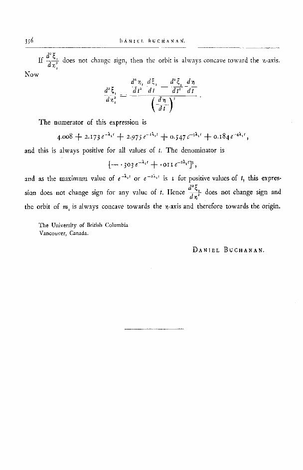
The three asymptotic orbits are always concave to the origin. The proofs of this are entirely similar for the three orbits, so only the orbit of m, will be consi- dered.

The coordinates of m are given by the equations

~, = x , cos n t - - y , s in n t,

~, = x, sin n t + y~ eos n t,

#, ----" " - 3.474 + o,jI5 e "'''4~ + O, I85e -1'68~ ,

~ ~ 0.226 e -x'34~ -- 0,oo4 r176 ,

~56 DANIEL BUCHANAN ~.

If ~ does not change sign, then the orbit is always concave toward the "a-axis.

Now

d ~ , _ d t a d t d t 2 d t

\-aT-! The numerator of this expression is

4.008 -~- 2. i73e-Z, ' -+- 2.975 e-2Z, ' -at- o.547c-3Z, ' + o.I84 e-*z'',

and this is always positive for all values of t. The denominator is

[--" 303 e -z'' + " oI I e-2Z,'] ' ,

and as the maximum value of e -x'' or e -2x,' is I for positive values of t, this expres-

sion does not change sign for any value of t. Hence d '~ , does not change sign and

the orbit of m, is always concave towards the x-axis and therefore towards the origin.

The University of British Columbia Vancouver, Canada.

DANIEL BUCHANAN.