Orbital localization using fourth central moment minimizationIda-Marie Høyvik, Branislav Jansik, and Poul Jørgensen

Citation: The Journal of Chemical Physics 137, 224114 (2012); doi: 10.1063/1.4769866View online: http://dx.doi.org/10.1063/1.4769866View Table of Contents: http://aip.scitation.org/toc/jcp/137/22Published by the American Institute of Physics

Articles you may be interested inLocalized molecular orbitals for polyatomic molecules. I. A comparison of the Edmiston-Ruedenberg and Boyslocalization methodsThe Journal of Chemical Physics 61, 3905 (2003); 10.1063/1.1681683

A fast intrinsic localization procedure applicable for ab initio and semiempirical linear combination of atomicorbital wave functionsThe Journal of Chemical Physics 90, 4916 (1998); 10.1063/1.456588

Incremental full configuration interactionThe Journal of Chemical Physics 146, 104102 (2017); 10.1063/1.4977727

Localization of open-shell molecular orbitals via least change from fragments to moleculeThe Journal of Chemical Physics 146, 104104 (2017); 10.1063/1.4977929

THE JOURNAL OF CHEMICAL PHYSICS 137, 224114 (2012)

Orbital localization using fourth central moment minimizationIda-Marie Høyvik,1 Branislav Jansik,2 and Poul Jørgensen1

1qLEAP Center for Theoretical Chemistry, Department of Chemistry, Aarhus University, Langelandsgade 140,Aarhus 8000, Denmark2VSB-TUO, 17. listopadu 15/2172, 798 33 Ostrava-Poruba, Czech Republic

(Received 12 October 2012; accepted 13 November 2012; published online 14 December 2012)

We present a new orbital localization function based on the sum of the fourth central moments of theorbitals. To improve the locality, we impose a power on the fourth central moment to act as a penaltyon the least local orbitals. With power two, the occupied and virtual Hartree-Fock orbitals exhibit amore rapid tail decay than orbitals from other localization schemes, making them suitable for use inlocal correlation methods. We propose that the standard orbital spread (the square root of the secondcentral moment) and fourth moment orbital spread (the fourth root of the fourth central moment) areused as complementary measures to characterize the locality of an orbital, irrespective of localizationscheme. © 2012 American Institute of Physics. [http://dx.doi.org/10.1063/1.4769866]

I. INTRODUCTION

It is a basic assumption in local correlation methods thatthe wave function is expanded in a set of local orbitals. How-ever, which criteria a set of orbitals have to fulfill in or-der to be characterized as local is not clear. In one of thepopular textbooks in computational chemistry,1 local orbitalsare defined as orbitals “that are spatially confined to a rela-tively small volume, and therefore clearly displaying whichatoms are bonded and furthermore have the property of be-ing approximately constant between structurally similar unitsin different molecules.” Locality is here intimately associ-ated with molecular bonding and connected to the struc-tural similarity of the chemical units in different molecules.In the Pipek–Mezey orbital localization scheme,2, 3 the ideais to reduce the number of atomic sites for a bonding or-bital. The close connection between locality and chemicalbonding is widely accepted despite the fact that molecularbonding is associated with the nodal structure of an orbitaland with particular sets of orbitals, e.g., HOMO-LUMO gapand Koopman’s theorem for canonical Hartree–Fock (HF)orbitals.

In the context of local correlation methods, local or-bitals are introduced with the sole purpose of providing a lo-cal basis where the short range inter-electronic interactions(Coulomb holes and dispersion forces) can be described ef-ficiently. For such a purpose, it is only important to use or-bitals that are confined to a small volume in space, and theirbonding properties are irrelevant. The problem is how to findappropriate criteria for determining and characterizing localorbitals.

A vast number of localization schemes (e.g., Refs. 3–13) have been proposed since Lennard-Jones and Pople14

published an article on localized occupied orbitals andtheir physical meaning in 1950. The most used localizationschemes are the ones of Boys,4, 5 Edmiston and Ruedenberg,6

and Pipek and Mezey.2, 3 In solid state physics, the Boysand Pipek–Mezey schemes have been employed to obtain

maximally localized Wannier orbitals.15, 16 The use of theBoys, Pipek–Mezey, and Edmiston–Ruedenberg schemes toobtain a local virtual orbital space has been very limited,due to the failure of the Jacobi sweeps of iterations6 to op-timize the functions for the virtual space. Projected atomicorbitals (PAOs), which constitute a redundant non-orthogonalset, have been used in some local correlation methods17–19

in the absence of local virtual HF orbitals. Recently, Høyviket al.20 showed that a set of local, non-redundant orthonor-mal virtual orbitals can be obtained by using the trust regionoptimization of the localization functions.

The Boys scheme minimizes the sum of the second cen-tral moments (variances) of the orbitals. For simplicity, wewill refer to the second central moment as the second moment.The second moment of an orbital characterizes the deviationof its density from its average position, and hence measureswhere the bulk of the orbital density is located. The Boys lo-calization thus produces a set of orbitals, which on averageare local, but the set may contain some orbitals, which have alarge second moment—so-called outliers. For a set of orbitals,it is the locality of the least local orbital (“the weakest link”)that defines the locality of the set. Jansik et al.12 showed howoutliers could be removed by imposing a power on the secondmoments, acting as a penalty for orbitals with large secondmoments.

When minimizing the second moment, no considerationsare given to the shape of the orbital, except that the bulk of theorbital is concentrated in a small volume of space. However,a small second moment may be obtained because of an acutepeak and a thick tail or because of a broad peak and a thin tail.In local correlation methods, local orbitals must have a thintail since only then is the orbital really restricted to a smallvolume in space. In this paper, we describe how local orbitalswith a fast tail decay may be obtained by minimizing the sumof the fourth moments for a set of orbitals. To avoid outliersin the fourth moment minimization, we further suggest to im-pose a power on the fourth moment in accordance with thepower on the second moment as discussed in Ref. 12.

0021-9606/2012/137(22)/224114/11/$30.00 © 2012 American Institute of Physics137, 224114-1

224114-2 Høyvik, Jansik, and Jørgensen J. Chem. Phys. 137, 224114 (2012)

The second moment of an orbital is used to characterizethe locality of an orbital since it reflects the spatial confine-ment of the bulk of the orbital. In practice, the orbital spread,which is the square root of the second moment of the orbital,is reported. In this paper, we will refer to the orbital spreadas the second moment orbital spread (σ 2) to distinguish itfrom what we term the fourth moment orbital spread (σ 4),which is the fourth root of the fourth moment of the orbital. σ 4

provides a second essential characterization of the locality ofan orbital, which reflects more directly the thickness of theorbital tail than σ 2 does. Thus, to fully characterize the local-ity of a set of orbitals, we suggest to report σ 2 and σ 4 for themost de-local orbitals (orbitals with the greatest σ 2 and σ 4) inthe set.

In Sec. II, we develop the localization function for thefourth moment minimization, and in Sec. III, we derivethe equations needed for a minimization of the fourth mo-ment localization function using the trust region method. InSec. IV, we present results for orbitals obtained using a fourthmoment minimization. The orbitals are compared to the or-bitals obtained from a second moment minimization both withand without imposed powers, and also with Pipek–Mezey lo-calizations. Section V contains a summary and some conclud-ing remarks.

II. SECOND AND QUARTIC MOMENTLOCALIZATION FUNCTIONS

The locality of an orbital |p〉 = φp can be associated withits second moment (variance). In one dimension, the secondmoment of the orbital is defined as

μp

2 = 〈p|(x − 〈p|x|p〉)2|p〉 =∫

(x − xp)2φ∗pφpdx, (1)

where∫

φ∗pφpdx = 1 and xp = ∫

xφ∗pφpdx. The second mo-

ment of an orbital is thus defined in terms of an integrationof the density φ∗

pφp over a second moment weight function(x − xp)2. A local orbital has a small second moment sincethe bulk of the orbital—represented by its density—will beclose to its average position.

For a set of orbitals {|p〉, |q〉· · · } (e.g., a set of occupiedor virtual HF orbitals), the set which on average is most localmay be obtained using the Boys localization scheme wherethe second moment (SM) localization function

ξSM =∑

p

μp

2 (2)

is minimized carrying out a sequence of orthogonal transfor-mations between the orbitals. When ξSM is minimized, theorbitals are rotated in order to get their deviation from themean position xp to be as small as possible. Positions far fromxp (where |x − xp| � 0) are given a large weight and the or-bitals therefore are rotated to get a density, which is small inthis region. The Boys localization is thus in that sense directlydirected toward getting orbitals, where the bulk of the orbitalis confined to a small volume in space. The second momentorbital spread of orbital |p〉

σp

2 =√

μp

2 , (3)

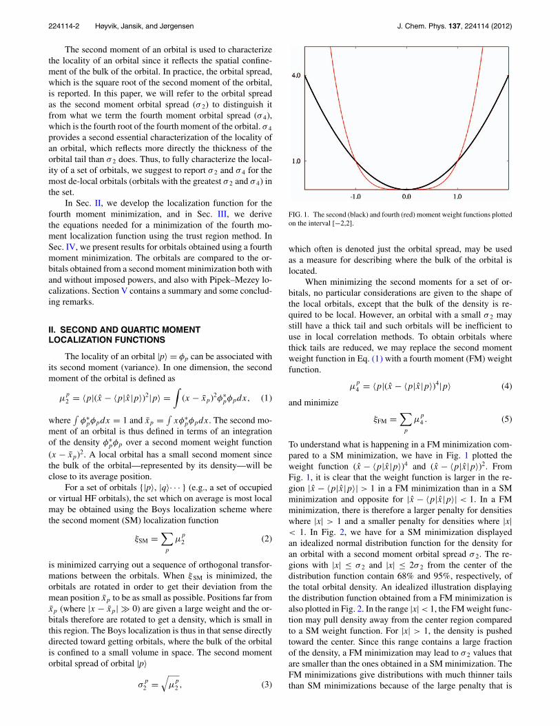
FIG. 1. The second (black) and fourth (red) moment weight functions plottedon the interval [−2,2].

which often is denoted just the orbital spread, may be usedas a measure for describing where the bulk of the orbital islocated.

When minimizing the second moments for a set of or-bitals, no particular considerations are given to the shape ofthe local orbitals, except that the bulk of the density is re-quired to be local. However, an orbital with a small σ 2 maystill have a thick tail and such orbitals will be inefficient touse in local correlation methods. To obtain orbitals wherethick tails are reduced, we may replace the second momentweight function in Eq. (1) with a fourth moment (FM) weightfunction.

μp

4 = 〈p|(x − 〈p|x|p〉)4|p〉 (4)

and minimize

ξFM =∑

p

μp

4 . (5)

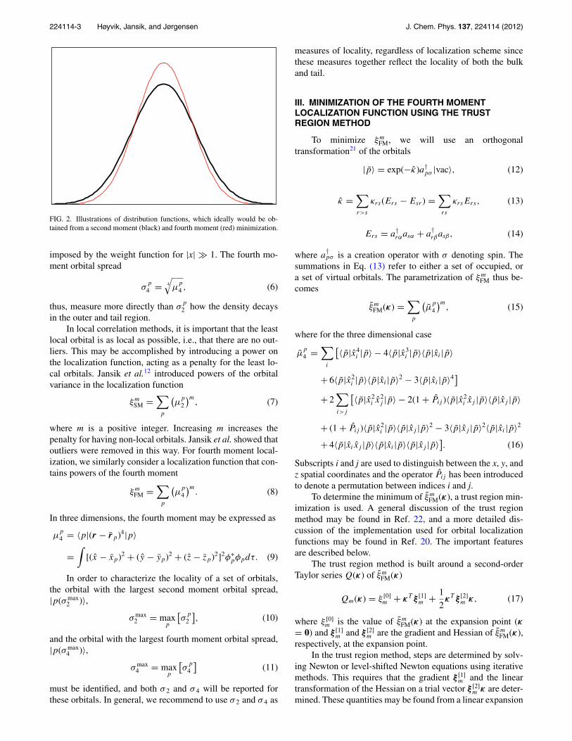
To understand what is happening in a FM minimization com-pared to a SM minimization, we have in Fig. 1 plotted theweight function (x − 〈p|x|p〉)4 and (x − 〈p|x|p〉)2. FromFig. 1, it is clear that the weight function is larger in the re-gion |x − 〈p|x|p〉| > 1 in a FM minimization than in a SMminimization and opposite for |x − 〈p|x|p〉| < 1. In a FMminimization, there is therefore a larger penalty for densitieswhere |x| > 1 and a smaller penalty for densities where |x|< 1. In Fig. 2, we have for a SM minimization displayedan idealized normal distribution function for the density foran orbital with a second moment orbital spread σ 2. The re-gions with |x| ≤ σ 2 and |x| ≤ 2σ 2 from the center of thedistribution function contain 68% and 95%, respectively, ofthe total orbital density. An idealized illustration displayingthe distribution function obtained from a FM minimization isalso plotted in Fig. 2. In the range |x| < 1, the FM weight func-tion may pull density away from the center region comparedto a SM weight function. For |x| > 1, the density is pushedtoward the center. Since this range contains a large fractionof the density, a FM minimization may lead to σ 2 values thatare smaller than the ones obtained in a SM minimization. TheFM minimizations give distributions with much thinner tailsthan SM minimizations because of the large penalty that is

224114-3 Høyvik, Jansik, and Jørgensen J. Chem. Phys. 137, 224114 (2012)

FIG. 2. Illustrations of distribution functions, which ideally would be ob-tained from a second moment (black) and fourth moment (red) minimization.

imposed by the weight function for |x| � 1. The fourth mo-ment orbital spread

σp

4 = 4

√μ

p

4 , (6)

thus, measure more directly than σp

2 how the density decaysin the outer and tail region.

In local correlation methods, it is important that the leastlocal orbital is as local as possible, i.e., that there are no out-liers. This may be accomplished by introducing a power onthe localization function, acting as a penalty for the least lo-cal orbitals. Jansik et al.12 introduced powers of the orbitalvariance in the localization function

ξmSM =

∑p

(μ

p

2

)m, (7)

where m is a positive integer. Increasing m increases thepenalty for having non-local orbitals. Jansik et al. showed thatoutliers were removed in this way. For fourth moment local-ization, we similarly consider a localization function that con-tains powers of the fourth moment

ξmFM =

∑p

(μ

p

4

)m. (8)

In three dimensions, the fourth moment may be expressed as

μp

4 = 〈p|(r − rp)4|p〉

=∫

[(x − xp)2 + (y − yp)2 + (z − zp)2]2φ∗pφpdτ. (9)

In order to characterize the locality of a set of orbitals,the orbital with the largest second moment orbital spread,|p(σ max

2 )〉,σ max

2 = maxp

[σ

p

2

], (10)

and the orbital with the largest fourth moment orbital spread,|p(σ max

4 )〉,σ max

4 = maxp

[σ

p

4

](11)

must be identified, and both σ 2 and σ 4 will be reported forthese orbitals. In general, we recommend to use σ 2 and σ 4 as

measures of locality, regardless of localization scheme sincethese measures together reflect the locality of both the bulkand tail.

III. MINIMIZATION OF THE FOURTH MOMENTLOCALIZATION FUNCTION USING THE TRUSTREGION METHOD

To minimize ξmFM, we will use an orthogonal

transformation21 of the orbitals

|p〉 = exp(−κ)a†pσ |vac〉, (12)

κ =∑r>s

κrs(Ers − Esr ) =∑rs

κrsErs, (13)

Ers = a†rαasα + a

†rβasβ, (14)

where a†pσ is a creation operator with σ denoting spin. The

summations in Eq. (13) refer to either a set of occupied, ora set of virtual orbitals. The parametrization of ξm

FM thus be-comes

ξmFM(κ) =

∑p

(μ

p

4

)m, (15)

where for the three dimensional case

μp

4 =∑

i

[〈p|x4i |p〉 − 4〈p|x3

i |p〉〈p|xi |p〉

+ 6〈p|x2i |p〉〈p|xi |p〉2 − 3〈p|xi |p〉4

]

+ 2∑i>j

[〈p|x2i x

2j |p〉 − 2(1 + Pij )〈p|x2

i xj |p〉〈p|xj |p〉

+ (1 + Pij )〈p|x2i |p〉〈p|xj |p〉2 − 3〈p|xj |p〉2〈p|xi |p〉2

+ 4〈p|xi xj |p〉〈p|xi |p〉〈p|xj |p〉]. (16)

Subscripts i and j are used to distinguish between the x, y, andz spatial coordinates and the operator Pij has been introducedto denote a permutation between indices i and j.

To determine the minimum of ξmFM(κ), a trust region min-

imization is used. A general discussion of the trust regionmethod may be found in Ref. 22, and a more detailed dis-cussion of the implementation used for orbital localizationfunctions may be found in Ref. 20. The important featuresare described below.

The trust region method is built around a second-orderTaylor series Q(κ) of ξm

FM(κ)

Qm(κ) = ξ [0]m + κT ξ [1]

m + 1

2κT ξ [2]

m κ, (17)

where ξ [0]m is the value of ξm

FM(κ) at the expansion point (κ= 0) and ξ [1]

m and ξ [2]m are the gradient and Hessian of ξm

FM(κ),respectively, at the expansion point.

In the trust region method, steps are determined by solv-ing Newton or level-shifted Newton equations using iterativemethods. This requires that the gradient ξ [1]

m and the lineartransformation of the Hessian on a trial vector ξ [2]

m κ are deter-mined. These quantities may be found from a linear expansion

224114-4 Høyvik, Jansik, and Jørgensen J. Chem. Phys. 137, 224114 (2012)

of ∂ξmFM

∂κkl.

∂ξmFM

∂κkl

= m∑

p

(μ

p

4

)m−1 ∂μp

4

∂κkl

, (18)

where μp

4 is given in Eq. (16) and m is a positive integer. Thelinear expansions of the individual terms in Eq. (18) usingκ = 0 as the expansion point are given by

(μ

p

4

)m−1 = f [0]p + κT f [1]

P + O(κ2), (19)

∂(μ

p

4

)∂κkl

= (g[0]

p

)kl

+ (κT g[1]

p

)kl

+ O(κ2). (20)

Using Eq. (16), expressions for f [0]p , κT f [1]

P , (g[0]p )kl , and

(κT g[1]p )kl are found. The gradient is not dependent on κ and

from the expansions above, we may find the gradient as(ξ [0]

m

)kl

= m∑

p

f [0]p

(g[0]

p

)kl. (21)

The linear transformations of the Hessian on a trial vector κ

consist of the terms in the expansion that depend linearly onκ and may be found from(ξ [2]

m κ)kl

= m∑

p

[f [0]

p

(κT g[1]

p

)kl

+ (κT f [1]

p

)(g[0]

p

)kl

]. (22)

The explicit expressions for the gradient and linear trans-formation of the Hessian on a trial vector are listed in theAppendix.

IV. RESULTS

In this section, we report results from fourth moment or-bital localizations for various molecular systems. σ 2 and σ 4

are computed for all orbitals, and the locality of an orbitalset is described in terms of σ 2 and σ 4 for the orbital in theset with the largest σ 2, |p(σ max

2 )〉, and for the orbital with thelargest σ 4, |p(σ max

4 )〉. Arachidic acid (C20O2H40) is used as anexample of a one-dimensional system and the I27SS domain(C124N36O37S3H192) of the titin protein as a three-dimensionalexample. We will for simplicity refer to the I27SS domain oftitin as just titin. In all calculations, we will employ Dun-ning’s correlation consistent basis sets cc-pVXZ23 with car-dinal numbers X = D, T, and Q. All starting orbitals used arethe least-change orbitals of Ziolkowski et al.,11 and the local-izations were performed using a trust region minimization.20

No convergence issues were encountered, and for a detailedaccount on convergence rates for localization functions, werefer to Ref. 20.

In Sec. IV A, we compare the locality measures of or-bitals that are obtained in a FM and SM minimization usingpowers m = 1, 2, and 3, to investigate the effect of m. InSec. IV B, the shape of the bulk and tail regions in FMand SM minimization are analyzed. For both Secs. IV A andIV B, we focus on examining the locality of the virtual or-bitals since these are much more difficult to localize thanthe occupied orbitals. In Sec. IV C, FM localization withm = 2 as penalty is compared to Boys and Pipek–Mezeylocalizations for a variety of molecular systems. All orbital

TABLE I. σ 2 and σ 4 values for the virtual orbitals of arachidic acid withσmax

2 and σmax4 listed for various basis sets and localization criteria.

DZ TZ QZ

σ 2 (a.u.) σ 4 (a.u.) σ 2 (a.u.) σ 4 (a.u.) σ 2 (a.u.) σ 4 (a.u.)

ξ1FM |p(σmax

2 )〉 2.70 3.37 2.99 3.75 2.98 4.27|p(σmax

4 )〉 2.35 3.43 2.62 3.84 2.87 4.42

ξ2FM |p(σmax

2 )〉 2.26 2.94 2.18 2.84 2.20 3.02|p(σmax

4 )〉 2.16 3.03 2.09 2.98 2.18 3.02

ξ3FM |p(σmax

2 )〉 2.25 2.92 2.17 2.82 2.12 2.81|p(σmax

4 )〉 2.15 2.95 2.07 2.91 2.11 2.94

ξ1SM |p(σmax

2 )〉 3.19 3.99 3.57 4.55 3.81 5.08|p(σmax

4 )〉 3.19 3.99 3.03 4.59 3.31 5.12

ξ2SM |p(σmax

2 )〉 2.36 3.40 2.43 3.66 2.53 3.49|p(σmax

4 )〉 2.35 3.46 2.42 3.66 2.45 3.66

ξ3SM |p(σmax

2 )〉 2.26 3.22 2.24 3.31 2.14 3.17|p(σmax

4 )〉 2.26 3.27 2.24 3.31 2.03 3.25

PAO |p(σmax2 )〉 3.13 3.40 3.49 3.76 3.82 4.11

|p(σmax4 )〉 2.90 3.79 3.49 3.76 3.82 4.11

visualizations are created using the UCSF Chimera programpackage.24

A. Investigating effects of the power m

We will now investigate the effect of an increasing powerm on the FM localization function. In Table I, we report theresult of a ξm

FM, m = 1, 2, and 3, minimization of the virtualorbitals for arachidic acid for cardinal numbers X = D, T, andQ. We report the locality measures σ 2 and σ 4 for |p(σ max

2 )〉and |p(σ max

4 )〉. For comparison, we also report locality resultsfrom a ξm

SM, m = 1, 2, and 3 minimization, and the locality ofthe PAOs.

From Table I, we see that σ max2 and σ max

4 changes dras-tically when going from m = 1 to m = 2, but do not changemuch when increasing m from 2 to 3. |p(σ max

2 )〉 and |p(σ max4 )〉

have similar σ 2 and σ 4 values. In fact, the distribution of or-bitals with σ 2 and σ 4 values in the maximum region is ratherdense, as can be seen from the plots in Figs. 3 and 4 whereσ 2 and σ 4 are displayed for all virtual orbitals obtained fromFM and SM minimizations, respectively, for m = 1 (top), 2(middle), and 3 (bottom) and using the cc-pVTZ basis set.Figs. 3 and 4 substantiate that it is important to impose apenalty (use m = 2) but increasing this penalty (use m = 3)has only minor effects. This observation is in accordance withthe experience from ξ 2

SM localizations,12 where it was foundthat m = 2 was a sufficient penalty. From Fig. 3, we also seethat for the FM localizations with m = 2, all virtual orbitalshave σ 2 values close to 2.0 a.u. and σ 4 values slightly below3.0 a.u., leaving little space for improving the locality by con-sidering higher than fourth moment localizations.

For titin, results—similar to the ones for arachidic acid—are reported in Table II. The trends for the titin results are thesame as for arachidic acid, even though the shifts in local-ity going from m = 1 to m = 2 are larger for titin than forarachidic acid.

224114-5 Høyvik, Jansik, and Jørgensen J. Chem. Phys. 137, 224114 (2012)

FIG. 3. σ 2 (left) and σ 4 (right) plotted for all virtual orbitals of arachidicacid in a cc-pVTZ basis localized using ξ1

FM (top), ξ2FM (middle), and ξ3

FM(bottom).

For the occupied orbitals, we observe trends similar tothe ones for the virtual orbitals even though the effects forthe occupied orbitals are less pronounced than for the virtualorbitals. As a conclusion, we recommend to use m = 2 for FMlocalizations.

B. The locality of orbitals in fourth momentminimization

In this section, we examine in more detail the orbital lo-cality obtained from a FM minimization with m = 2, i.e., us-ing ξ 2

FM. For comparison, we present results using ξ 2SM. We

start out considering the locality for the virtual orbitals, wherewe also present the locality of PAOs. Then we examine the

FIG. 4. σ 2 (left) and σ 4 (right) plotted for all virtual orbitals of arachidicacid in a cc-pVTZ basis localized using ξ1

SM (top), ξ2SM (middle), and ξ3

SM(bottom).

TABLE II. σ 2 and σ 4 values for the virtual orbitals of titin with σmax2 and

σmax4 listed for various basis sets and localization criteria.

DZ TZ

σ 2 (a.u.) σ 4 (a.u.) σ 2 (a.u.) σ 4 (a.u.)

ξ1FM |p(σmax

2 )〉 3.40 4.06 3.91 5.16|p(σmax

4 )〉 3.26 4.35 3.73 5.18

ξ2FM |p(σmax

2 )〉 2.47 3.08 2.45 3.14|p(σmax

4 )〉 2.42 3.16 2.43 3.21

ξ3FM |p(σmax

2 )〉 2.46 3.04 2.40 3.10|p(σmax

4 )〉 2.40 3.10 2.38 3.11

ξ1SM |p(σmax

2 )〉 3.48 4.21 3.92 5.00|p(σmax

4 )〉 3.21 4.35 3.62 5.21

ξ2SM |p(σmax

2 )〉 2.71 3.34 2.76 3.84|p(σmax

4 )〉 2.60 3.62 2.76 3.84

ξ3SM |p(σmax

2 )〉 2.52 3.41 2.49 3.33|p(σmax

4 )〉 2.52 3.41 2.19 3.46

PAO |p(σmax2 )〉 4.71 5.63 3.68 4.15

|p(σmax4 )〉 4.65 5.63 2.94 4.50

locality of the obtained occupied orbitals. For the occupiedorbitals, we only present results for titin, since the arachidicacid occupied orbitals are much less complicated and easilylocalized.

1. Virtual orbitals

We will now compare the locality of the virtual orbitalsobtained in ξ 2

FM and ξ 2SM localizations for arachidic acid. We

first consider the difference in tail decay between FM and SMoptimized orbitals. To do this, we have in Fig. 5 for a ξ 2

FM min-imization in a cc-pVTZ basis plotted the virtual orbital withthe largest fourth moment spread, |p(σ max

4 )〉, (σ 2 = 2.09 a.u.,σ 4 = 2.98 a.u.) for the contour values 0.03, 0.003, and 0.001.

FIG. 5. The least local virtual orbital |p(σmax4 )〉 (σ 2 = 2.09 a.u. and σ 4

= 2.98 a.u.) for arachidic acid in a cc-pVTZ basis obtained from a ξ2FM min-

imization plotted using contour values 0.03 (top), 0.003 (middle), and 0.001(bottom). A box representing the orbital of Fig. 6 is superimposed to illustratethe more rapid tail decay of the fourth moment optimized orbitals.

224114-6 Høyvik, Jansik, and Jørgensen J. Chem. Phys. 137, 224114 (2012)

FIG. 6. The virtual orbital centered at the same position as the orbital inFig. 5 but obtained from a ξ2

SM localization (σ 2 = 2.41 a.u. and σ 4 = 3.63)for arachidic acid in a cc-pVTZ basis, plotted using contour values 0.03 (top),0.003 (middle), and 0.001 (bottom). A box encasing the orbital is added touse for comparison against the orbital presented in Fig. 5.

For comparison, we have in Fig. 6 plotted the orbital that ina ξ 2

SM minimization is centered on the same carbon atom asthe orbital in Fig. 5. This orbital has σ 2 = 2.41 a.u. and σ 4

= 3.63 a.u. For the contour values 0.003 and 0.001, we havefor the SM optimized orbital (Fig. 6), drawn a black linemarking the boundary of the orbital. The boundary is super-imposed on the FM optimized orbital in Fig. 5. From Fig. 5,we clearly see that the ξ 2

FM optimized orbital exhibits a more

rapid tail decay than the ξ 2SM optimized orbital (boundary of

ξ 2SM optimized orbital is denoted by the black line).

To get more insight into the structure of the FM andSM minimized orbitals and their different tail decay, wehave in Fig. 7 plotted the distribution functions (left) and thecumulative distribution functions (right) for the orbitals ofFigs. 5 and 6 where the integration is performed along theinternuclear axis. σ 2 along the nuclear axis is 1.22 a.u. forthe FM optimized orbital and 1.49 a.u. for the SM optimizedorbital. In Fig. 7 (left), we have also plotted an idealizedone-dimensional normal distribution function for the SM op-timized orbital (σ 2 = 1.49 a.u.). From Fig. 7, we see that theidealized distribution function is broader than the distributionfunction obtained from integration over the SM and FM op-timized orbitals. This occurs because the penalty m = 2 thatis imposed on the orbitals forces the density toward the or-bital center both in the SM and the FM localization. For thecumulative distribution functions, the more rapid tail decay isreflected by the fact that the cumulative distribution functionfor the FM optimized orbital approaches the Heaviside stepfunction more than the SM optimized orbital does, emphasiz-ing that density is being pushed from the tail region towardthe center region for the FM optimized orbitals.

Looking at the results in Table I, we see that the FMminimization in general gives lower σ max

2 values than a SMminimization. For example, for a TZ basis, FM minimizationusing m = 2 gives σ max

2 = 2.18 a.u., while a SM minimiza-tion using m = 2 gives σ max

2 = 2.43 a.u. At a first glance,this is a peculiar result since σ 2 (via μ

p

2 ) is directly mini-mized in a SM minimization, but not in a FM minimization.The observation is understood from the theoretical analysis inSec. II, which showed that the bulk of the density obtained

0

0.1

0.2

0.3

0.4

0.5

0.6

-4.0 -2.0 0.0 2.0 4.0

Dis

trib

utio

n

Displacement from center of orbital (a.u.)

Second moment, m=2Fourth moment, m=2

Normal distribution

0

0.2

0.4

0.6

0.8

1

-4.0 -2.0 0.0 2.0 4.0

Cum

ulat

ive

dist

ribu

tion

Displacement from center of orbital (a.u.)

FIG. 7. The distribution functions (left) and cumulative distribution functions (right) for the orbitals plotted in Fig. 5 (red curve) and Fig. 6 (black curve). Inaddition, a normal distribution (dashed line) with the same orbital spread along the internuclear axis as the orbital represented by the black curve is illustrated.

224114-7 Høyvik, Jansik, and Jørgensen J. Chem. Phys. 137, 224114 (2012)

FIG. 8. The most de-local virtual orbital |p(σmax4 )〉 (σmax

2 = 2.42 a.u.,σmax

4 = 3.16 a.u.) for titin in a cc-pVDZ basis obtained from a ξ2FM mini-

mization plotted using contour values 0.03 (top), 0.003 (middle), and 0.001(bottom). The box which was encasing the orbitals shown in Fig. 9 is super-imposed to illustrate the more rapid tail decay of the fourth moment opti-mized orbitals.

from a FM minimization will be more compact compared toa SM minimization, because the density is pushed toward thecenter region in a FM minimization.

We also examine the locality for the virtual orbitals oftitin obtained using a ξ 2

FM optimization. From Table II, wesee that for the cc-pVDZ basis σ max

2 = 2.47 a.u. and σ max4

= 3.16 a.u. from a ξ 2FM minimization, while the correspond-

ing numbers are σ max2 = 2.71 a.u. and σ max

4 = 3.62 a.u. froma ξ 2

SM minimization. Both the maximum values for σ 2 and σ 4

are thus reduced in a FM minimization compared to a SMminimization. In Figs. 8 and 9, we have plotted the orbitalswith σ max

4 for a ξ 2FM and a ξ 2

SM minimization, respectively.The results from Table II and from Figs. 8 and 9 confirmthat the trends observed for arachidic acid are also found fortitin. For example, the orbital plot in Fig. 8 clearly shows howthe tail is reduced in a FM localization compared to a SMlocalization. Comparing the σ max

2 and σ max4 values obtained

from a FM minimzation with the locality of the PAOs for titin

FIG. 9. The most de-local virtual orbital |p(σmax4 )〉 (σmax

2 = 2.60 a.u.,σmax

4 = 3.62 a.u.) for titin in a cc-pVDZ basis obtained from a ξ2SM mini-

mization plotted using contour values 0.03 (top), 0.003 (middle), and 0.001(bottom). A box encasing the orbital is added to use for comparison againstthe orbitals presented in Fig. 8.

(Table II), we see that the PAOs are much less local than FMlocalized orbitals.

2. Occupied orbitals

We now proceed to examine the locality of the occupiedorbitals obtained from a FM minimization. In Table III, wegive locality results for the valence orbitals of titin. As seenfrom Table III, σ 2 and σ 4 are very similar whether a SM or

TABLE III. σ 2 and σ 4 values for the occupied orbitals with σmax2 and σmax

4of titin in various basis sets.

DZ TZ

σ 2 (a.u.) σ 4 (a.u.) σ 2 (a.u.) σ 4 (a.u.)

ξ2FM |p(σmax

2 )〉 2.20 2.91 2.21 2.72|p(σmax

4 )〉 2.20 2.91 2.20 2.91

ξ2SM |p(σmax

2 )〉 2.19 2.94 2.20 2.96|p(σmax

4 )〉 2.19 2.94 2.19 2.96

224114-8 Høyvik, Jansik, and Jørgensen J. Chem. Phys. 137, 224114 (2012)

TABLE IV. σ 2 and σ 4 values for the virtual orbitals with σmax2 and σmax

4 for various molecules.

ξ2FM Boys (ξ1

SM) Pipek–Mezey

σ 2 (a.u.) σ 4 (a.u.) σ 2 (a.u.) σ 4 (a.u.) σ 2 (a.u.) σ 4 (a.u.)

Alanine20/cc-pvDZ |p(σmax2 )〉 2.22 2.82 3.32 4.26 3.63 4.33

|p(σmax4 )〉 2.20 3.02 3.32 4.26 3.48 4.40

Alanine20/cc-pvTZ |p(σmax2 )〉 2.17 2.89 3.72 4.74 4.28 5.40

|p(σmax4 )〉 1.99 2.91 3.49 4.94 4.26 5.40

Aβ1 − 42/cc-pVDZ |p(σmax2 )〉 2.46 3.03 3.53 4.32 4.11 5.48

|p(σmax4 )〉 2.38 3.14 3.32 4.44 4.11 5.48

C60/cc-pVTZ |p(σmax2 )〉 2.27 3.23 3.23 4.46 5.05 6.30

|p(σmax4 )〉 2.25 3.24 2.92 4.55 5.05 6.30

Insulin/cc-pVDZ |p(σmax2 )〉 2.49 3.07 2.58 3.54 4.16 5.57

|p(σmax4 )〉 2.38 3.33 3.35 4.48 4.16 5.57

Graphene/cc-pVDZ |p(σmax2 )〉 2.63 3.58 3.10 4.32 4.55 5.93

|p(σmax4 )〉 2.51 3.65 2.71 4.69 3.66 6.92

a FM localization is carried out. However, when the orbitalsare studied in greater detail, we see that tails are reduced if afourth moment minimization is carried out.

C. Fourth moment localization compared to Boys andPipek–Mezey localizations

In this section, we compare the locality of orbital setsfor various molecular systems, using a ξ 2

FM localization andusing Boys and Pipek–Mezey localizations. Boys and Pipek–Mezey localizations have so far been the preferred localiza-tion schemes for obtaining local orbitals. The molecules con-sidered are:

� An alpha-helix containing 20 alanine residues, denotedalanine(20), in a cc-pVDZ and cc-pVTZ basis (1924and 4458 basis functions, respectively).

� The amyloid β-peptide Aβ1–4225 in a cc-pVDZ basis

(6106 basis functions).� A graphene sheet (C106H28) in a cc-pVDZ basis (1624

basis functions).

� C60 in a cc-pVTZ basis (1800 basis functions).� Insulin (C257N65O77S6H−

382) in a cc-pVDZ basis (7604basis functions).

In Table IV, we report the locality for the virtual orbitalsfor the molecular systems described above. From Table IV,it is seen that the locality of ξ 2

FM localized virtual orbitalshas a rather narrow range for the different molecular systemsand also when increasing the cardinal number of the basissets. The Boys and Pipek–Mezey localized orbitals are seento be less local than the ξ 2

FM localized orbitals and also show-ing a larger range for σ max

2 and σ max4 values for the different

molecular systems. For example, the σ max2 values in Table IV

for ξ 2FM localizations are in the range 2.17–2.63 a.u., while

for Boys and Pipek–Mezey localizations the range is 2.58–3.72 a.u. and 3.63–5.05 a.u., respectively. For σ max

4 , the rangeis 2.91–3.65 a.u. for ξ 2

FM localizations, while it is 4.16–4.94 a.u. and 4.40–6.92 a.u. for Boys and Pipek–Mezey lo-calizations, respectively.

In Table V, we report localization results for the occu-pied orbitals of the molecular systems described above. The

TABLE V. σ 2 and σ 4 values for the occupied orbitals with σmax2 and σmax

4 for various molecules.

ξ2FM Boys (ξ1

SM) Pipek–Mezey

σ 2 (a.u.) σ 4 (a.u.) σ 2 (a.u.) σ 4 (a.u.) σ 2 (a.u.) σ 4 (a.u.)

Alanine20/cc-pvDZ |p(σmax2 )〉 1.62 2.15 1.70 2.25 1.90 2.43

|p(σmax4 )〉 1.59 2.18 1.70 2.25 1.90 2.43

Alanine20/cc-pvTZ |p(σmax2 )〉 1.61 2.15 1.72 2.29 1.90 2.44

|p(σmax4 )〉 1.58 2.16 1.72 2.29 1.90 2.44

Aβ1 − 42/cc-pVDZ |p(σmax2 )〉 2.16 2.65 2.12 2.86 2.73 3.24

|p(σmax4 )〉 2.14 2.77 2.12 2.86 2.72 3.25

C60/cc-pVTZ |p(σmax2 )〉 2.22 3.24 2.36 3.45 2.91 3.91

|p(σmax4 )〉 2.22 3.24 2.36 3.45 2.91 3.91

Insulin/cc-pVDZ |p(σmax2 )〉 2.17 2.67 2.17 2.89 2.76 3.25

|p(σmax4 )〉 2.15 2.78 2.17 2.89 2.72 3.26

Graphene/cc-pVDZ |p(σmax2 )〉 2.58 4.15 3.37 5.60 3.83 7.25

|p(σmax4 )〉 2.54 4.17 3.37 5.60 3.83 7.25

224114-9 Høyvik, Jansik, and Jørgensen J. Chem. Phys. 137, 224114 (2012)

results are presented as for the virtual orbitals reported inTable IV. The results show that a ξ 2

FM localization yieldsthe most local occupied orbitals. When comparing the threeschemes, the differences between the locality for the occu-pied orbitals are generally not as big as for the virtual or-bitals. However, it is important to note that for some sys-tems (e.g., graphene), the Boys and Pipek–Mezey localiza-tion schemes provide very poor locality for the occupied or-bitals. Thus, when using these schemes it is extremely im-portant to check the locality of the obtained orbitals, sincethey may yield only semi-local orbitals for some molecularsystems.

V. SUMMARY AND CONCLUDING REMARKS

We have introduced a localization function for occupiedand virtual orbitals based on powers of the orbital fourth mo-ment. The power is introduced to act as a penalty on the leastlocal orbitals, i.e., to ensure that no orbitals in the set aresignificantly less local than the others. It is shown that theorbitals obtained from a fourth moment minimization withpower m have a more rapid tail decay than orbitals obtainedfrom a second moment (Boys) minimization with the samepower m. Further, the improvement in tail decay is much morepronounced for the virtual than for the occupied orbitals. Apenalty value m = 2 was shown to be sufficient to obtain a setof orbitals in which all orbitals are properly local. A FM min-imization with a penalty m = 2 thus may be recommended forobtaining a set of local HF orbitals for local correlation

methods. Further, we propose that for any localizationscheme, the locality of the orbitals should be characterizedby the second and fourth moment orbital spreads of the leastlocal orbitals in the set.

ACKNOWLEDGMENTS

The research leading to these results has received fund-ing from the European Research Council under the EuropeanUnion’s Seventh Framework Programme (FP/2007-2013)/ERC (Grant Agreement No. 291371). The work has also beensupported by the Lundbeck Foundation, the Danish Center forScientific Computing (DCSC).

APPENDIX: EXPRESSIONS FOR GRADIENTAND LINEAR TRANSFORMATION OF HESSIANON TRIAL VECTOR

Expanding Eq. (18), inserting the results into Eqs. (21)and (22), and introducing the odd component of a matrix A as

{A}o = A − AT , (A1)

and defining dia[v] as the operation for taking a vector v andtransforming it to a diagonal matrix Dv containing the vectorelements on the diagonal

dia[v] = Dv, (A2)

we arrive at the following expressions for the gradient ξ [1]m and

linear transformation ξ [2]m κ :

ξ [1]m = m

∑i

[ − 2{

x4i dia[(μ4)m−1]

}o

+ 8{

x3i dia[(μ4)m−1xi]

}o − 12{

x2i dia[(μ4)m−1[xi]

2]}o

+ 8{

xidia[(μ4)m−1

[x3

i

]]}o − 24{

xidia[(μ4)m−1

[x2

i

]xi

]}o

+ 24{xidia[(μ4)m−1[xi]3]}o]

+ 2∑i>j

[ − {x2

i x2j dia[(μ4)m−1]

}o

− 8{xi xj dia[(μ4)m−1xi xj ]}o

− 4(1 + Pij ){

xj dia[(μ4)m−1[x2

i

]xj

]}o

+ 4(1 + Pij ){

xj dia[(μ4)m−1

[x2

i xj

]]}o

+ 12(1 + Pij ){xj dia[(μ4)m−1[xi]2xj ]}o

− 8(1 + Pij ){xj dia[(μ4)m−1xi[xi xj ]]}o

− 2(1 + Pij ){

x2i dia[(μ4)m−1[xj ]2]

}o

+ 4(1 + Pij ){

x2j xidia[(μ4)m−1xi]

}o], (A3)

224114-10 Høyvik, Jansik, and Jørgensen J. Chem. Phys. 137, 224114 (2012)

ξ [2]m κ = m

∑x=x,y,z

[ − 2{(κx4 − x4κ)dia[(μ4)m−1]}o

+ 8{x3dia[(μ4)m−1(κx − xκ)]}o + 8{(κx3 − x3κ)dia[(μ4)m−1x]}o

+ 8{xdia[(μ4)m−1(κx3 − x3κ)}o − 24{xdia[(μ4)m−1(κx2 − x2κ)x}o

− 24{xdia[(μ4)m−1[x2](κx − xκ)}o + 72{xdia[(μ4)m−1[x]2(κx − xκ)]}o

+ 8{(κx − xκ)dia[(μ4)m−1[x3]}o − 24{(κx − xκ)dia[(μ4)m−1x[x2]}o

+ 24(κx − xκ)dia[(μ4)m−1[x]3]}o − 24{x2dia[(μ4)m−1x(κx − xκ)]}o

− 12{(κx2 − x2κ)dia[(μ4)m−1[x]2]}o

− 2{x4dia[κT f [1]]}o + 8{x3dia[(κT f [1])x]}o

− 12{x2dia[(κT f [1])[x]2]}o + 8{xdia[(κT f [1])[x3]]}o

− 24{xdia[(κT f [1])[x2]x]}o + 24{xdia[(κT f [1])[x]3]}o]

+ 2m∑i>j

[ − 2{(

κx2i x2

j − x2i x2

jκ)dia[ f [0]}o

− 8{(κxi xj − xi xjκ)dia[ f [0]xi xj ]}o + (1 + Pij ){

xj dia[

f [0][x2i

](κxj − xjκ)

]}o

− 4(1 + Pij ){

xj dia[

f [0](κx2i − x2

i κ)xj

]}o + 4(1 + Pij ){

xj dia[

f [0](κx2i xj − x2

i xjκ)]}o

+ 24(1 + Pij ){xj dia[ f [0][xj ][xi](κxi − xiκ)]}o − 8(1 + Pij ){xj dia[ f [0]xi(κxi xj − xi xjκ)]}o

− 8(1 + Pij ){xj dia[ f [0]xi(κxi − xiκ)[xi xj ]]}o − 4(1 + Pij ){(κxj − xjκ)dia

[f [0][x2

i

]xj

]}o

+ 4(1 + Pij ){(κxj − xjκ)dia

[f [0][x2

i xj

]}o + 12(1 + Pij ){(κxj − xjκ)dia[ f [0][xi]2xj ]}o

− 8(1 + Pij ){(κxj − xjκ)dia[ f [0][xi xj ]xi]}o − 4(1 + Pij ){

x2i dia[ f [0](κxj − xjκ)xj ]

}o

− 2(1 + Pij ){(

κx2j − x2

jκ)dia[ f [0][xi]

2}o + 4(1 + Pij ){(

κx2i xj − x2

i xjκ)dia[ f [0]xj ]

}o

+ 4(1 + Pij ){

x2i xj dia[ f [0](κxj − xjκ)]

}o − 8(1 + Pij ){xi xj dia[ f [0](κxi − xiκ)xj ]}o

+ 2m∑i>j

[ − 2{

x2i x2

j dia[κT f [1]]}o − 8{xi xj dia[(κT f [1])xi xj ]}o

− 4(1 + Pij ){

xj dia[(κT f [1])[x2

i ]xj

]}o + 12(1 + Pij ){

xj dia[(κT f [1])[xi]2xj ]

}o

4(1 + Pij ){

xj dia[(κT f [1])[x2

i xj ]]}o − 2(1 + Pij ){x2

i dia[(κT f [1])[xj ]2]}o

+ 4(1 + Pij ){

x2i xj dia[(κT f [1])xj ]

}o]

− 1

2

{κξ [0]

m

}o. (A4)

Subscripts i and j are used to distinguish between the x,y, and z spatial coordinates and the operator Pij has been in-troduced to denote a permutation between indices i and j. Thecartesian moment matrix xn

i is defined by

xni =

∑p,q

〈p|xni |q〉. (A5)

In Table VI, we have specified the dimensions of the quanti-ties entering Eqs. (A3) and (A4).

For the gradient (Eq. (A3)), there are no matrix-matrixmultiplications, only vector-matrix operations. The linear

TABLE VI. The dimension of the quantities entering the gradient and thelinear transformation of the Hessian on a trial vector. Norb is the number oforbitals in the set. Note: all vectors are defined to be row vectors.

Quantity Dimensions

ξ[1]m Norb × Norb

ξ[2]m κ Norb × Norb

κ Norb × Norb

xni Norb × Norb

κxni Norb × Norb

(μ4)m−1 1 × Norb

f [0] 1 × Norb

κT f [1] 1 × Norb

224114-11 Høyvik, Jansik, and Jørgensen J. Chem. Phys. 137, 224114 (2012)

transformation of the Hessian on a trial vector (Eq. (A4)) con-tains 25 matrix-matrix multiplications. One multiplication isthe gradient multiplied with the trial vector and the remaining24 are multiplications of each of the cartesian moment matri-ces with the trial vector.

All matrix operations are implemented in parallel anddistributed fashion using the block cyclic distribution of dataand the ScaLAPACK library.26 Interprocess communicationis done via the message passing interface (MPI) of the MPI

library.27 This allows us to utilize the combined processorpower and memory of several computational nodes in de-manding evaluations of the linear transformation. The paral-lelization enables fourth moment minimization to be appliedto large molecules with reasonably sized basis sets.

1F. Jensen, Introduction to Computational Chemistry, 2nd ed. (Wiley, 2007).2J. Pipek, Int. J. Quantum Chem. 36, 487 (1989).3J. Pipek and P. G. Mezey, J. Chem. Phys. 90, 4916 (1989).4S. F. Boys, Rev. Mod. Phys. 32, 296 (1960).5S. F. Boys, Quantum Theory of Atoms, Molecules and Solid State (Aca-demic, New York, 1966), p. 253.

6C. Edmiston and K. Ruedenberg, Rev. Mod. Phys. 35, 457 (1963).7W. von Niessen, J. Chem. Phys. 56, 4290 (1972).8J. E. Subotnik, A. D. Dutoi, and M. Head-Gordon, J. Chem. Phys. 123,114108 (2005).

9F. Aquilante, T. Pedersen, A. S. de Meras, and H. Koch, J. Chem. Phys.125, 174101 (2006).

10V. Weber and J. Hutter, J. Chem. Phys. 128, 064107 (2008).

11M. Ziółkowski, B. Jansík, P. Jørgensen, and J. Olsen, J. Chem. Phys. 131,124112 (2009).

12B. Jansík, S. Høst, K. Kristensen, and P. Jørgensen, J. Chem. Phys. 134,194104 (2011).

13P. de Silva, M. Giebultowski, and J. Korchowiec, Phys. Chem. Chem. Phys.14, 546 (2012).

14J. E. Lennard-Jones and J. A. Pople, Proc. R. Soc. London 202, 166 (1950).15G. Berghold, C. J. Mundy, A. H. Romero, J. Hutter, and M. Parrinello,

Phys. Rev. B 61, 10040 (2000).16I. Souza, N. Marzari, and D. Vanderbilt, Phys. Rev. B 65, 35109 (2002).17S. Saebø and P. Pulay, Ann. Rev. Phys. Chem. 44, 213 (1993).18M. Schütz, G. Hetzer, and H.-J. Werner, J. Chem. Phys. 111, 5691 (1999).19M. Schütz and H.-J. Werner, J. Chem. Phys. 114, 661 (2001).20I.-M. Høyvik, B. Jansik, and P. Jørgensen, J. Chem. Theory Comput. 8,

3137 (2012).21T. Helgaker, P. Jørgensen, and J. Olsen, Molecular Electronic Structure

Theory, 1st ed. (Wiley, 2000).22R. Fletcher, Practical Methods of Optimization, 2nd ed. (Wiley, Chichester,

1987).23T. H. Dunning, Jr., J. Chem. Phys. 90, 1007 (1989).24E. Pettersen, T. Goddard, C. Huang, G. Couch, D. Greenblatt, E. Meng, and

T. Ferrin, J. Comput. Chem. 13, 1605 (2004).25B. Strodel, J. W. L. Lee, C. S. Whittleston, and D. J. Wales, J. Am. Chem.

Soc. 132, 13300 (2010).26L. S. Blackford, J. Choi, A. Cleary, E. D’Azevedo, J. Demmel, I. Dhillon,

J. Dongarra, S. Hammarling, G. Henry, A. Petitet et al., ScaLAPACK Users’Guide (Society for Industrial and Applied Mathematics, Philadelphia, PA,1997).

27E. Gabriel, G. E. Fagg, G. Bosilca, T. Angskun, J. J. Dongarra, J. M.Squyres, V. Sahay, P. Kambadur, B. Barrett, A. Lumsdaine et al., in Pro-ceedings of the 11th European PVM/MPI Users’ Group Meeting on OpenMPI: Goals, Concept, and Design of a Next Generation MPI Implementa-tion (Euro PVM/MPI, Budapest, Hungary, 2004).