1

ORBITAL LIFETIME ANALYSES OF PICO- AND NANO-SATELLITES

By

AI-AI LUMNAY C. COJUANGCO

A THESIS PRESENTED TO THE GRADUATE SCHOOL OF THE UNIVERSITY OF FLORIDA IN PARTIAL FULFILLMENT

OF THE REQUIREMENTS FOR THE DEGREE OF MASTER OF SCIENCE

UNIVERSITY OF FLORIDA

2007

2

© 2007 Ai-Ai Lumnay C. Cojuangco

3

To my mother and sister

4

ACKNOWLEDGMENTS

I extend my sincere gratitude to my advisor, Dr. Norman Fitz-Coy, for his generous

support, guidance and patience through my graduate studies at the University of Florida.

I acknowledge and give appreciation to my committee members Dr. John K. Schueller and

Dr. Carl Crane for providing valuable input to this work.

I acknowledge my colleagues in the AMAS lab, the Space Systems Group and SAMM

group, for their support, input, and company with research and graduate studies.

I express my appreciation to the women in my life group, Pascalie Belony, Jamie Cabug,

Ann Duong, Sunny Ho, Jenny Jose, Christine Moran, and Carrie Torbert for their continuous

encouragement, belief in me, words of wisdom, prayers, and for being such great inspirations to

my life since I arrived at University of Florida. Also, to all the wonderful people I have met and

befriended through Gator Christian Life.

I thank Cris Dancel for her time, guidance and support with this work. I also express my

appreciation to the rest of the Filipino community I have met here for making me feel at home. I

thank my friends in Illinois as well for keeping me in their thoughts.

I thank my family. I especially thank my mother, Evangeline Chongco, and sister,

Claudine Foronda, for their love, support, and for allowing me to pursue graduate studies.

Last, I express my deep gratitude to Jesus Christ, my Lord, my Savior and my God, it is

through Him I have faith and strength and it is He who has made all of this possible. I thank

Him for his beautiful creation that I have had the joy in living and learning about.

5

TABLE OF CONTENTS page

ACKNOWLEDGMENTS ...............................................................................................................4

LIST OF TABLES...........................................................................................................................7

LIST OF FIGURES .........................................................................................................................8

ABSTRACT.....................................................................................................................................9

CHAPTER

1 INTRODUCTION AND BACKGROUND ...........................................................................11

Definition of Orbital Debris....................................................................................................11 Concerns with Orbital Debris .................................................................................................11 Development of Mitigation Guidelines ..................................................................................15 Motivation of Research...........................................................................................................17

2 METHODS.............................................................................................................................20

Two-body Problem .................................................................................................................20 Conic Sections ........................................................................................................................23 Orbital Elements .....................................................................................................................25 Perturbations ...........................................................................................................................26 Perturbation Techniques .........................................................................................................30 Orbital Lifetime ......................................................................................................................33

3 SIMULATIONS USING SATELLITE TOOL KIT (STK) SOFTWARE.............................35

Satellite Tool Kit (STK) .........................................................................................................35 STK Lifetime Tool .................................................................................................................35 STK Satellite Properties .........................................................................................................39 Parameter Sensitivity Study....................................................................................................41

4 RESULTS AND DISCUSSION.............................................................................................46

Pico-satellite Results...............................................................................................................46 Nano-satellites Results............................................................................................................50

5 CONCLUSION AND RECOMMENDATIONS ...................................................................58

Conclusions.............................................................................................................................58 Recommendations...................................................................................................................59

6

LIST OF REFERENCES...............................................................................................................60

BIOGRAPHICAL SKETCH .........................................................................................................63

7

LIST OF TABLES

Table page 3-1 Satellite mass, drag area, and area exposed to Sun..........................................................37

3-2 Orbital lifetime sensitivity simulation parameters...........................................................41

4-1 CubeSat simulation parameters........................................................................................47

4-2 MR SAT and MRS SAT simulation parameters..............................................................51

4-3 FASTRAC simulation parameters ...................................................................................51

4-4 Akoya-B and Bandit-C simulation parameters ................................................................52

4-5 MR SAT with different initial altitudes simulation parameters.......................................52

8

LIST OF FIGURES

Figure page 1-1 Typical pico- and nano-class satellite mass, volume and power ratios ...........................18

1-2 Computer generated image of orbital debris in LEO.......................................................19

2-1 Relative motion of two-bodies.........................................................................................21

2-2 Geometry of an elliptic conic section ..............................................................................24

2-3 Orbital elements ...............................................................................................................25

3-1 STK Lifetime tool GUI....................................................................................................36

3-2 STK Lifetime Advanced option GUI...............................................................................39

3-3 STK satellite properties GUI ...........................................................................................40

3-4 Orbital lifetime vs. reflection coefficient.........................................................................43

3-5 Orbital lifetime vs. area exposed to Sun ..........................................................................43

3-6 Orbital lifetime vs. drag coefficient .................................................................................44

3-7 Orbital lifetime vs. drag area ...........................................................................................44

3-8 Orbital lifetime vs. mass ..................................................................................................45

4-1 Orbital lifetime results for satellite A using seven atmospheric density models.............48

4-2 Orbital lifetime results for satellite C using seven atmospheric density models .............48

4-3 Orbital lifetime results for satellites A, B, C, and D at 600-km initial altitude ...............49

4-4 Orbital lifetime for MR SAT and MRS SAT at 350-km initial altitude..........................54

4-5 Orbital lifetime for MR SAT and MRS SAT at 750-km initial altitude..........................55

4-6 Orbital lifetime for the FASTRAC satellites at 350-km initial altitude...........................55

4-7 Orbital lifetime for the FASTRAC satellites at 750-km initial altitude...........................56

4-8 Orbital lifetime for the Akoya-B and Bandit-C at 350-km initial altitude ......................56

4-9 Orbital lifetime for the Akoya-B and Bandit-C at 750-km initial altitude ......................57

4-10 Orbital lifetime for the MR SAT using different initial altitudes ....................................57

9

Abstract of Thesis Presented to the Graduate School of the University of Florida in Partial Fulfillment of the

Requirements for the Degree of Master of Science

ORBITAL LIFETIME ANALYSES OF PICO- AND NANO-SATELLITES

By

Ai-Ai Lumnay C. Cojuangco

December 2007

Chair: Norman Fitz-Coy Major: Mechanical Engineering

In recent years, orbital debris has been a growing concern for the space industry due to its

potential risk of causing collisions. Several agencies and organizations, such as the National

Aeronautics and Space Administration (NASA), and the United Nations Committee on the

Peaceful Uses of Outer Space (UNCOPUOS), have been involved in studying orbital debris and

developing mitigation guidelines. In 2004, the Federal Communications Commission (FCC)

began requiring a debris mitigation plan for all non-government United States radio

communication satellites to be launched into orbit.

Orbital lifetime analysis of a satellite is important in its development and in complying

with debris mitigation guidelines. Factors that must be taken into consideration include

environmental perturbations, such as solar radiation pressure, the Earth’s oblateness, and

atmospheric drag. Other factors that affect orbital lifetime prediction are the satellite’s physical

properties. In this research, these perturbations and their effects on orbital lifetime, for Earth-

orbiting satellites, were investigated.

In this study, orbital lifetimes were determined using the Lifetime analysis tool in

Analytical Graphics’ Satellite Tool Kit (STK) software, focusing on pico- and nano-satellites.

The focus on these two classes of satellites is due to their perceived rapid growth and the

10

potential difficulty of adhering to FCC requirements for debris mitigation. The effect of solar

cycle and different atmospheric density models were also explored during the analyses.

The results indicate that orbital lifetimes of pico-satellites can be significantly reduced by

increasing their drag area. For instance, changing the drag area of a 1-kg satellite from 0.01 to

0.1 m2 decreased its orbital lifetime from 22 to 3 years, an 86% reduction. At 600 km above the

Earth’s surface, pico-satellites with drag areas of 0.1 m2 had minimum orbital lifetimes during

years of highest solar activity. Our analysis implies that passive de-orbiting devices such as drag

chutes can be effective devices on pico-satellites for addressing orbital debris mitigation.

Meanwhile, the nano-satellites used in our study were between 11 to 28 kg, with drag areas from

0.08 and 0.2 m2, which led to orbital lifetimes in centuries when launched at 750 km altitude.

Values indicate that additions to the nano-satellites are needed to fulfill a 25 year orbital lifetime

requirement set by the FCC.

11

CHAPTER 1 INTRODUCTION AND BACKGROUND

Definition of Orbital Debris

The launch of Sputnik in 1957 was the dawn of space exploration and a significant

milestone in the advances in science and technology. Since that date, numerous missions and

manned spacecraft have been launched and continue to be launched for scientific, educational,

and technological purposes. A major effect not considered in the early years of space

exploration was the contribution of artificial bodies (i.e., spent satellites and spacecraft

components) to the debris population in space. Two categories of debris now exist, natural (i.e.,

meteoroids) and artificial (i.e., used rocket bodies). Artificial debris is also referred to as orbital

debris. Orbital debris refers to man made space objects that are no longer functioning or serve

any useful purpose. Prior practices and procedures have allowed unregulated growth of orbital

debris, however, in recent years, the issue of orbital debris has become extremely important

requiring that the space industry monitors debris orbiting the Earth and develop procedures to

curtail its growth in the future.1

Concerns with Orbital Debris

There are several factors that have and will contribute to the growth of orbital debris, the

primary contributors being (1) explosions, (2) prior practices and procedures that have involved

the abandonment of spacecraft and upper stages, (3) the deposition rate of objects being sent into

space, (4) collisions, and (5) future trends of small satellite usage by academia, government and

industry.

First, orbital debris growth’s primary cause is explosions, which produce breakups or

fragments. Explosions can be accidental or intentional. Accidental explosions obtain energy

from on-board energy sources. Meanwhile, intentional explosions include tests (i.e., anti-

12

satellite testing) or spacecraft separation. For example, in low Earth orbit (LEO), altitudes up to

2,000 km above the Earth’s surface, accidental explosions of spent upper stages have been the

main source of debris.2

Second, the next largest contributor to orbital debris has been prior practices and

procedures that involved the abandonment of spacecraft and upper stages in their current orbit

after the spacecraft has completed its mission or is no longer operational. The National

Aeronautics and Space Administration (NASA) reported in 1995 the accumulation of

approximately 1968 tons of orbital debris due to these practices.2

Third, assets are being launched into space at a rate that is higher than the rate at which

expired assets are being removed by natural and artificial means.3 This has led to an average

growth rate in debris population of 5% per annum in LEO.4

Fourth, a major concern to orbital debris growth is collisions. Collisions can occur

between varieties of satellite classes. Due to their large speeds, when space objects collide with

each other, they may become non-operational. These masses would spatially distribute

themselves producing debris fragments or debris clouds and thus add on to the total debris

population. The threat of these clouds is evident by the debris created from the recently

destroyed Chinese satellite, Fengyun 1-C, this past January 2007.

Last, research and trends in the past were focused on traditional large costly satellites, but

are now transitioning to smaller satellites. This trend is the result of these satellites potential

lower costs and advances in technology, which allows for miniaturization. The Defense

Advanced Research Projects Agency (DARPA) organization is exploring fractionated spacecraft

flying in formation as well as a collection of heterogeneous small satellite modules5 performing

various tasks. This trend is also seen in academia through projects such as the CubeSat and the

13

University Nano-satellite Program (UNP).

The CubeSat program was developed by the California Polytechnic State University in San

Luis Obispo, and Stanford University’s Space Systems Development lab as a mechanism to

enable universities to participate in the design, launch, and operations of satellites at an

affordable cost.6 A one unit CubeSat is a 10×10×10 cm cube with a mass of 1 kg classified as a

pico- satellite. Currently, these satellites typically have short operational lifetimes as compared

to their orbital lifetimes and if not properly disposed after its primary mission will then

contribute orbital debris.

The UNP is a joint program composing of the Air Force Research Laboratory’s Space

Vehicles Directorate (AFRL/VS), the Air Force Office of Scientific Research (AFOSR), and the

American Institute of Aeronautics and Astronautics (AIAA). The program is a national student

satellite design and fabrication competition. It also enables small satellite research and

development, integration, payload development, and flight tests.7 There are a growing number

of these satellite classes planned on being sent to space and the increase can potentially

contribute to the total amount in number and mass of the orbital debris population.

The growth of orbital debris has become an immediate issue as its presence in space

continues to have an impact with the utilization of space assets. It is continuously monitored and

modeled by agencies such as NASA and the United Nations Committee on the Peaceful Uses of

Outer Space (UNCOPUOS) for study and risk assessment to future space missions. The impact,

both immediate and lasting, of collisions and explosions on the orbital debris population and

resultant hazards to space operations are discussed.

Explosions can produce debris fragments in large number and cause an operating

spacecraft to fail, as well as produce smaller debris fragments that may degrade its performance.

14

Other spacecraft, hundreds of kilometers away, may also be at a great risk from these fragments

due to their high velocities that may set them in very long orbit lifetimes.2

According to NASA, collision between large objects follows this scenario:

First, once collisions begin to occur, it will be almost impossible to halt the process and they will occur with increasing frequency—a process referred to as collisional cascading. Second, the energies in collisional breakup are much larger than in explosive breakup, in the megajoule (a few kilograms to TNT) to gigajoule (a few metric tons of TNT) range. This energy comes from the very large amount of chemical energy used to get objects into orbit. This large amount of expended energy creates many more debris fragments in all size ranges and spreads the debris over many hundreds of kilometers of altitude. This debris may hit other satellite surfaces, carrying impact energies of hundreds of megajoules per kilogram of impactor mass. At these energies, debris less than 1 mm in diameter, typically about 1 mg of mass, can penetrate an unshielded spacecraft surface and damage sensitive surfaces such as optics or thermal radiators; debris less than 1 cm (1 gm) can penetrate even a heavily shielded surface; and debris as small as 10 cm (1 kg) can cause a spacecraft to break up into debris fragments.2

Consequently, the risk of collision between debris and another object has become a close

concern. Abandoned spacecraft and upper stages are cases of large non-operational objects

already in space for which this type of collision can occur. Computer modeling indicates that

collisions between large objects in orbit will become a major source of debris within the next 3

decades, even if spacecraft launches were limited at 5 launches per year. The orbital debris that

will be produced from these collisions will be small particles that are large in number and are

capable of damage to operational spacecraft1.1,2

For the purpose of this research, collision of objects in LEO is the focus. In this orbit, the

standard impact velocity of medium-sized orbital debris with other objects is about 13 km/s, with

an explosive potential equal to 40 times its mass of TNT. For instance, a 1-cm-diameter

aluminum sphere, about 1.4 grams, has a kinetic energy equivalent to the energy released by the

explosion of 0.056 kg of TNT (about 0.24 MJ). A 10-cm aluminum sphere, on the other hand, is

equivalent to 56 kg of TNT (about 240 MJ). Therefore, in LEO, the energy released by small

debris pieces may severely damage or destroy many spacecraft systems.1

15

Development of Mitigation Guidelines

Assessments of potential risks involved with orbital debris have led to possible solutions

and abatement measures. Although removing abandoned spacecrafts, upper stages, and other

orbital debris may be the most effective means in avoiding future collisions, this is not cost

effective because it would require difficult maneuvering of objects in space7.2,8

Several national and international agencies/organizations are involved in orbital debris

assessment and mitigation. In 1993, the Inter-Agency Space Debris Coordination Committee

(IADC) was founded “to enable space agencies to exchange information on space debris research

activities, to review the progress of ongoing cooperative activities, to facilitate opportunities for

cooperation in space debris research and to identify debris mitigation options 8F”9. Members of the

IADC consists of NASA, the Italian Space Agency (ASI), the British National Space Centre

(BNSC), the Centre National d’Etudes Spatiales (CNES), the China National Space

Administration (CNSA), the Deutsches Zentrum fuer Luft-und Raumfahrt e.V. (DLR), the

European Space Agency (ESA), the Indian Space Research Organisation (ISRO), the Japan

Aerospace Exploration Agency (JAXA), the National Space Agency of Ukrain (NSAU), and the

Russian Aviation and Space Agency (Rosaviakosmos).

By February 1994, the United Nations (UN) Scientific and Technical Subcommittee

agreed that international cooperation was needed to minimize the potential impact of space

debris on future space missions125H.9 NASA issued a comprehensive set of orbital debris mitigation

guidelines in 19959F.10 The U.S. Government along with NASA, the Federal Aviation

Administration (FAA), the Department of Defense (DoD), and the Federal Communications

Commission (FCC) presented a set of orbital debris mitigation standard practices in a 1998 U.S.

Government Orbital Debris Workshop for Industry10F.11 Japan, France, Russia, and the European

Space Agency (ESA) and other countries, have since followed suit with their own guidelines126H.10

16

President Reagan issued a directive on national space policy requiring the limitation of

orbital debris accumulation on February 11 of the same year. This directive initiated the

collaborative work of the U.S. and other nations to learn more about orbital debris hazards and

management. An International Technical Working Group was established through this, which

helped influence nations with space activities to take action in limiting orbital debris127H.2

By the year 2001, the United States Government adopted its own guideline, U. S.

Government Orbital Debris Mitigation Standard Practices128H11F. 10,12 The IADC reached a consensus

on a set of guidelines that were formally presented to the Scientific and Technical Subcommittee

of the UNCOPUOS on February 2003 129H.10 In June 2004, the FCC issued its own set of mitigation

rules, Orbital Debris Notice, closely following the U. S. Government Orbital Debris Mitigation

Standard Practices12F.13

Several orbital debris mitigation guidelines have been in place after NASA’s lead.

NASA’s, the U.S. Government’s, the IADC’s and the FCC’s guidelines are summarized here

with a focus on post mission disposal in LEO, for the purpose of this thesis. NASA’s guideline

has three general options for post mission disposal in LEO which are (1) atmospheric re-entry,

(2) maneuvering to a storage orbit, and (3) direct retrieval. For option one, the guideline states to

maneuver a structure into an orbit where atmospheric drag, the main nongravitational force

acting on satellites in LEO13F,14 will cause its lifetime to decay within 25 years after the end of its

mission. The second option states to maneuver the spacecraft with final missions passing

through LEO to a disposal orbit defined to be between 2500 km to 35,288 km. The last option

states to perform a direct retrieval of the spacecraft from its orbit within 10 years after the end of

its mission130H.2

The U.S. Government guidelines has the same three options as NASA, but with the

17

inclusion of human casualty risk to be limited to no greater than 1 in 10,000 upon re-entry added

to option one; different disposal orbit definition for option two; and, the time period stated to be

“as soon as practical” given for option three131H.12 The IADC Space Debris Mitigation Guidelines

has a post mission disposal section for the LEO region. The guideline gives the option for space

systems to be disposed by de-orbiting, by direct re-entry, by maneuvering it to an orbit that

reduces its lifetime and by direct retrieval14F.15

The FCC, which has general authority over U.S. radio communications with the exception

of government radio stations, includes three methods for post mission disposal. One method is

direct retrieval, which the commission currently states little relevance for this option regarding

Commission-licensed space stations. Another method is to maneuver a spacecraft to a disposal

or storage orbit. The storage orbit is defined to be in perigee altitudes above 2000 km and apogee

altitudes below 19,700 as suggested for satellites in LEO. The FCC gives two procedures for the

atmospheric re-entry option: (1) to use the spacecraft’s propulsion to bring it further into the

Earth’s atmosphere and (2) to move the satellite to an orbit from which atmospheric drag will

cause its re-entry into the Earth’s atmosphere and that it will decay within 25 years after the end

of its mission. For continued affordable access to space, the FCC ruled that a satellite system

operator must submit an orbital debris mitigation plan before requesting space station

authorization132H.13

Motivation of Research

This research, in response to the FCC ruling, investigates the different parameters that

affect the orbital lifetime of pico- and nano-class satellites. These classes of satellites are

increasingly gaining attention throughout the space industry due to their potential low cost and

technological advances. The University of Florida has been involved with small satellite

research, in particular the CubeSat, since the fall of 2004. The nano-satellites developed through

18

the UNP are another example of the trend in academia moving towards small satellites. The

increase in number of these satellites being sent to space is a concern. The typical size, mass,

and power ratios of these two classes of satellites are shown in Figure 1-1.

Power ~ 2W

Power ~ 20W

30cm30cm

10cm10cm

1 kg

10 kg

Pico Nano Figure 1-1. Typical pico- and nano-class satellite mass, volume and power ratios

As of May 2007, there have been 17 of the pico-class satellites referred to as CubeSats

successfully launched in LEO and are namely15F16F:16,17

• 2003: AAU CubeSat by the Aalborg University, DTUSat by the Technical University of Denmark, CanX-1 by the University of Toronto SFL, CubeSat XI-IV by the University of Tokyo, Cute-1 by the Tokyo Institute of Technology Matunaga LSS

• 2005: NCube-2 by the University of Oslo (and others), UWE-1 by the University of Würzburg, CubeSat XI-V by the University of Tokyo

• 2006: Cute-1.7 by the Tokyo Institute of Technology Matunaga LSS, HITSat by the Hokkaido Institute of Technology

• 2007: AeroCube-2 by the Aerospace Corporation, CAPE-1 by the University of Louisiana, CP-3 and CP-4 by the California Polytechnic State University, CSTB-1 by the Boeing company, Libertad-1 by the Sergio Arboleda University, MAST by Tethers Unlimited

The CubeSat has a small mass and volume that can make a huge collision impact especially due

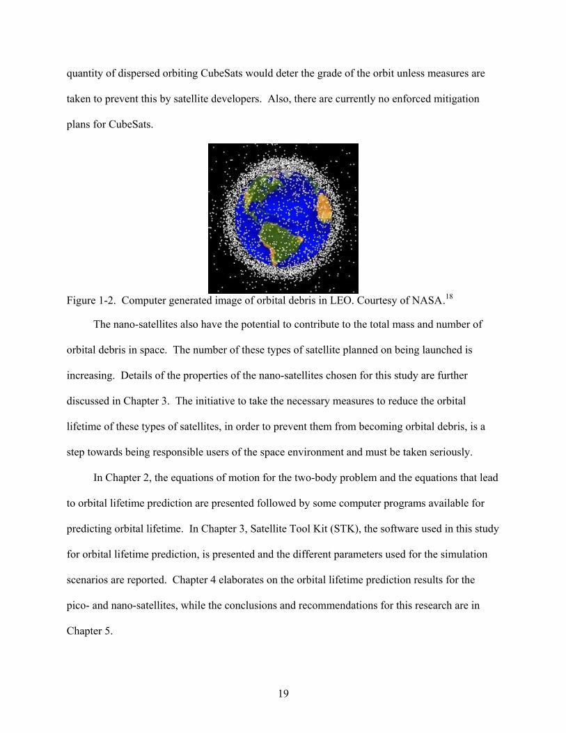
to both the high velocity rates and concentration of spacecrafts in LEO. Figure 1-2 shows a

computer generated image of the concentration of orbital debris that has been tracked in LEO

(2005) courtesy of NASA. As opportunities for CubeSats to access space continue to proliferate,

their contribution to the total mass may not seem substantial on a small scale. However, the

19

quantity of dispersed orbiting CubeSats would deter the grade of the orbit unless measures are

taken to prevent this by satellite developers. Also, there are currently no enforced mitigation

plans for CubeSats.

Figure 1-2. Computer generated image of orbital debris in LEO. Courtesy of NASA17F.18

The nano-satellites also have the potential to contribute to the total mass and number of

orbital debris in space. The number of these types of satellite planned on being launched is

increasing. Details of the properties of the nano-satellites chosen for this study are further

discussed in Chapter 3. The initiative to take the necessary measures to reduce the orbital

lifetime of these types of satellites, in order to prevent them from becoming orbital debris, is a

step towards being responsible users of the space environment and must be taken seriously.

In Chapter 2, the equations of motion for the two-body problem and the equations that lead

to orbital lifetime prediction are presented followed by some computer programs available for

predicting orbital lifetime. In Chapter 3, Satellite Tool Kit (STK), the software used in this study

for orbital lifetime prediction, is presented and the different parameters used for the simulation

scenarios are reported. Chapter 4 elaborates on the orbital lifetime prediction results for the

pico- and nano-satellites, while the conclusions and recommendations for this research are in

Chapter 5.

20

CHAPTER 2 METHODS

In this chapter the equation of motion for the two-body problem is discussed. Brief

summaries of conic sections and orbital elements are given. The equations of motion for the

two-body problem with perturbations are also presented. These equations are then used to

describe orbital lifetime. Some programs for orbital lifetime prediction are presented.

Two-body Problem

A model to describe a satellite’s orbital motion can be developed from planetary motions.

The physical motions of each planet were first described by Johannes Kepler’s three laws18F:19

• First Law – The orbit of each planet is an ellipse, with the sun at a focus.

• Second Law – The line joining the planet to the sun sweeps out equal areas in equal times.

• Third Law – The square of the period of a planet is proportional to the cube of its mean distance from the sun.

The first two laws of planetary motion were published in 1609, while the third in 1619. The

mathematical equations of planetary motions were not formulated until about 50 years later,

through Issac Newton’s second law of motion and law of universal gravitation. Newton’s

second law of motion states that “the rate of change of momentum is proportional to the force

impressed and is in the same direction as that force133H”19. Newton’s law of universal gravitation

states that “any two bodies attract one another with a force proportional to the product of their

masses and inversely proportional to the square of the distance between them 134H”19.

The equation for the second law of motion can be written as

2

2i i

i id r dvF m mdt dt

= ≡∑r rr

(2.1)

The notation F∑r

represents the sum of all the forces acting on a body which is equal to its

21

mass, im , times its acceleration, 2

2id r

dt

r

, measured relative to an inertial frame, and ivr is the

velocity vector. Newton’s law of universal gravitation can be written as

31

( ) 1,...n

i jg j i

j ijj i

m mF G r r i n

r=≠

= − =∑r r r (2.2)

where gFr

is the gravitational force on im due to jm and ( )j ir r−r r is the vector from im to jm .

The symbol G represents the universal gravitational constant and has the value of 6.670 × 10-8

dyne cm2/gm2135H.19

The equations of motion for planets and satellites were developed from equations 136H(2.1) and

137H(2.2). The equations of motion are applicable for a system of two bodies, referred to as the two-

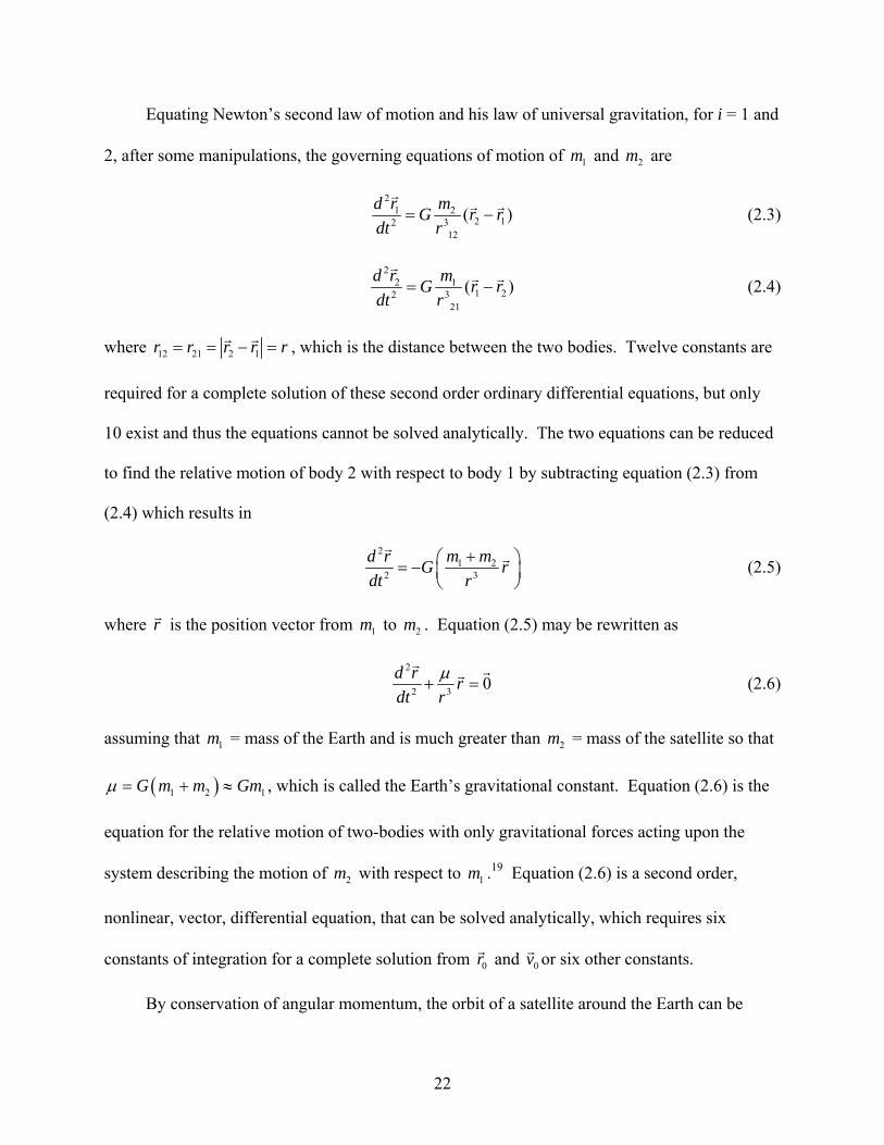
body problem, where n = 2 in equation 138H(2.2). An illustration of the system with bodies 1m and

2m is shown in Figure 2-1. Two assumptions are required to develop the equations of motion

and are as follows: (1) body 1 and body 2 are spherically symmetric (this allows for the bodies to

be treated as though the concentrations of their masses are at their centers) and (2) only

gravitational forces are acting on the system, which act along the line joining the centers of the

two bodies. An inertial reference frame is also defined to measure the motion. In Figure 2-1 the

set of inertial coordinates is defined by ( , ,X Y Z ). The position vectors of 1m and 2m , with

respect to the inertial frame, are defined as 1rr and 2r

r , respectively, so that 2 1r r r= −r r r

139H

.19

2m1m

rr

1rr

2rr

X

Z

Y

2m1m

rr

1rr

2rr

X

Z

Y

Figure 2-1. Relative motion of two-bodies

22

Equating Newton’s second law of motion and his law of universal gravitation, for i = 1 and

2, after some manipulations, the governing equations of motion of 1m and 2m are

2

1 22 12 3

12

( )d r mG r rdt r

= −r

r r (2.3)

2

2 11 22 3

21

( )d r mG r rdt r

= −r

r r (2.4)

where 12 21 2 1r r r r r= = − =r r , which is the distance between the two bodies. Twelve constants are

required for a complete solution of these second order ordinary differential equations, but only

10 exist and thus the equations cannot be solved analytically. The two equations can be reduced

to find the relative motion of body 2 with respect to body 1 by subtracting equation 140H(2.3) from

141H(2.4) which results in

2

1 22 3

m md r G rdt r

+⎛ ⎞= − ⎜ ⎟⎝ ⎠

rr (2.5)

where rr is the position vector from 1m to 2m142H

. Equation 143H(2.5) may be rewritten as

2

2 3 0d r rdt r

μ+ =

r rr (2.6)

assuming that 1m = mass of the Earth and is much greater than 2m = mass of the satellite so that

( )1 2 1G m m Gmμ = + ≈ , which is called the Earth’s gravitational constant. Equation 144H(2.6) is the

equation for the relative motion of two-bodies with only gravitational forces acting upon the

system describing the motion of 2m with respect to 1m145H

.19 Equation 146H(2.6) is a second order,

nonlinear, vector, differential equation, that can be solved analytically, which requires six

constants of integration for a complete solution from 0rr and 0vr or six other constants.

By conservation of angular momentum, the orbit of a satellite around the Earth can be

23

shown to lie on a plane. The angular momentum vector, hr

, is then perpendicular to the orbit

plane and is a constant vector. A partial solution to Equation 147H(2.6) is easy to obtain, that tells the

size and shape of the orbit. Crossing hr

to Equation 148H(2.6) leads to a form of equation that can be

integrated:

( )2

2 3

d r h h rdt r

μ× = ×

r r r r (2.7)

The left side of Equation 149H(2.7) equals d dr hdt dt⎛ ⎞×⎜ ⎟⎝ ⎠

r r and the right side equals 2

drv rr r dtμ μ

−r r and

after some manipulations Equation 150H(2.7) can be rewritten as

d dr d rhdt dt dt r

μ⎛ ⎞⎛ ⎞× =⎜ ⎟⎜ ⎟⎝ ⎠⎝ ⎠

r rr (2.8)

Integrating both sides results in

dr rh Bdt r

μ× = +r rr r

(2.9)

where Br

is a vector constant of integration. Dot multiplying Equation 151H(2.9) by rr results in a

scalar equation

2 cosh r rB fμ= + (2.10)

where f is the angle between Br

and rr . By solving for r , Equation 152H(2.10) becomes

( )

2 /1 / cos

hrB f

μμ

=+

(2.11)

and is called the trajectory equation expressed in polar coordinates153H.19

Conic Sections

Equation 154H(2.11) is similar to the equation of a conic section, where a conic section may be

defined as “a curve formed by the intersection of a plane passing through a right circular cone”14.

24

The equation of a conic section can be written as

1 cos

pre f

=+

(2.12)

and gives the magnitude of the position vector, r r=r , in terms of its location in the orbit where

p is called the parameter or semi-latus rectum, e is the eccentricity, and f is the polar angle or

true anomaly. The type of conic section represented by equation 155H(2.12) is determined by the

value of the eccentricity. When 0e = the conic section is a circle, 0 1e< < produces an ellipse,

1e = generates a parabola, and 1e > represents a hyperbola.

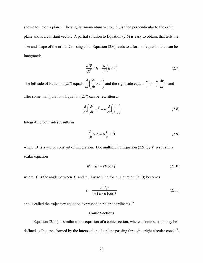
Figure 2-2 shows a geometric representation of an elliptic conic section. The figure shows

the conic section having two foci, where F is the primary focus (i.e., the Earth’s center) and 'F

is the secondary or vacant focus. C is the center of the ellipse. Half the distance between foci is

the dimension 'c . The dimension a is the semi-major axis and b is the semi-minor axis of the

ellipse. The distance from the primary focus to the farthest point of the ellipse is called the

radius of apogee, ar , and to the closest point of the ellipse is called the radius of perigee, pr .

From Kepler’s Second Law, the time required to complete one orbit is called the orbital period,

TP, and is expressed as

3/ 22TP aπμ

= (2.13)

'cC F'F

ar pr

bp

a

fr

'cC F'F

ar pr

bp

a

fr

Figure 2-2. Geometry of an elliptic conic section

25

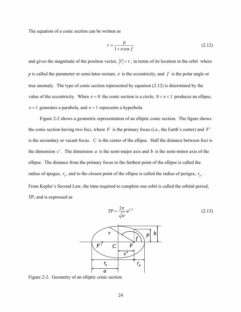
Orbital Elements

The six other constants of integration possible, asides from position and velocity for the

solution of Equation 156H(2.6), to describe the motion of a satellite around the Earth, are known as

orbital elements or Keplerian orbital elements as shown in Figure 2-3 and are defined below (See

reference 14).

• Semi-major axis ( a ) – Defines the size of the orbit.

• Eccentricity ( e ) – Defines the shape of the orbit.

• Inclination ( i ) – The angle between Zr

and angular momentum vector, hr

.

• Right Ascension of Ascending Node (RAAN) (Ω ) – “The angle from the vernal equinox to the ascending node. The ascending node is the point where the satellite passes through the equatorial plane moving from south to north. Right ascension is measured as a right-handed rotation about the pole, Z

r.”

• Argument of Perigee (ω ) – “The angle from the ascending node to the eccentricity vector, er , measured in the direction of the satellite’s motion. The eccentricity vector points from the center of the Earth to perigee with a magnitude equal to the eccentricity of the orbit.”

• Mean anomaly ( M ) – “The fraction of an orbit period which has elapsed since perigee, expressed as an angle. The mean anomaly equals the true anomaly for a circular orbit.”

Vernal EquinoxDirection

Line of Nodes

PeriapsisDirection

i

ω

0f

γ Xr

Yr

Zr

hr

0rr

er

Ω

Line of Nodes

(Always Defined)

PeriapsisDirection

Ω ω0f

γ(Always Defin

ed) 0r

Figure 2-3. Orbital elements

26

Perturbations

The amount of time a satellite remains in orbit before perturbations causes its reentry into

the Earth’s atmosphere is the satellite’s orbital lifetime and can be found from the sum of its

orbital period, TP. The orbital period is a function of the semi-major axis. When the semi-major

axis remains constant then the period is constant and the orbital lifetime is indefinite. Orbital

lifetime goes towards infinity as a increases because the period gets larger. Orbital lifetime

becomes finite when the semi-major axis decreases as this causes the period to decrease. The

duration of a satellite’s orbit with respect to the Earth is indefinite when the only forces acting on

the system are gravitational forces. The orbital elements also remain constant. When other

forces act on the system, however, the relative motion equation becomes

2

2 3 dd r r adt r

μ+ =

rr r (2.14)

where dar is the perturbing acceleration. This non-homogeneous differential equation implies

that the previous “constants of motion are no longer constant. Thus, orbital lifetime can be finite

when perturbations are considered. 20,21

Some of these perturbations are atmospheric drag, solar radiation pressure, the Earth’s

oblateness, and other bodies (n-body effect). Factors to consider with these perturbations are

solar activity, geomagnetic activity, atmospheric density, and ballistic coefficient (a function of

the satellite’s mass, mean cross sectional drag area, and drag coefficient). These perturbing

accelerations cause a satellite’s orbit to decrease and no longer be indefinite. The orbit will

decay into the Earth’s atmosphere and the time it takes for the decay to bring the satellite into the

Earth is the satellite’s orbital lifetime. In predicting the orbital lifetime of satellites,

perturbations must be taken into consideration. These factors and uncertainties in the solar and

27

geomagnetic activities can make orbital lifetime prediction very challenging19F20F.20,21 Some of the

factors that affect lifetime are discussed here.

The Earth’s upper atmosphere has a strong effect on satellites in space. The atmosphere is

dynamic and is affected mostly by the sun’s radiation. This solar activity heats up the

atmosphere and it expands as a result. The expansion “produces a variation in density

proportional to the degree of heating, which in turn depends upon solar activity21F”22. Solar activity

and Sun spots vary periodically, which is commonly known as the 11-year solar cycle. The

radiation from the sun is measured as a mean daily flux in the 10.7 cm (F10.7) wavelength in

solar flux units (sfu).

A bulge is also created, as a result of the heating on the side of the Earth that is facing the

sun. This causes “the density at a given point above the Earth to vary diurnally, as the point

rotates through the bulge every 24 hours, and seasonally, as the bulge moves with the sun in

latitude from winter to summer 157H”22. The atmosphere is influenced by geomagnetic activity as

well “through delayed heating of atmospheric particles from collisions with charged energetic

particles from the sun22F”23. Satellite lifetimes are affected most by the variation in the solar cycle

and the heat from radiation. Disturbances from geomagnetic activity are usually too short to

affect lifetimes significantly.14

Atmospheric drag is the main nongravitational force that acts on a satellite in LEO.14 Drag

is part of the total aerodynamic force that acts on a body moving through a fluid such as air158H.21 It

acts in the direction opposite of the velocity and takes away energy from the orbit. The decrease

in energy causes the orbit to decay until the satellite reenters the atmosphere. The equation for

the acceleration of a spacecraft due to drag is

212

dd r

C Aa vm

ρ ⎛ ⎞= − ⎜ ⎟⎝ ⎠

(2.15)

28

where ρ is the atmospheric density, dC is the satellite’s drag coefficient ≈ 2.2, A is the average

cross-sectional area of the satellite normal to its direction of travel (drag area) , m is the mass of

the satellite and rv is the satellite’s velocity relative to the atmosphere. The term d

mC A

is the

ballistic coefficient and is used as a measure of a satellite’s response to drag effects 159H.14,23 The

drag area is directly related to the satellite’s shape, dimensions and attitude motion160H.21 Mass is

usually taken to be constant during a satellite’s lifetime. When there is a mass loss, drag

deceleration of the satellite increases and its lifetime is shortened 161H.22 The ballistic coefficient can

indicate how fast a satellite will decay along with solar activity. Satellites with low ballistic

coefficients tend to decay more quickly in response to the atmosphere than those with high

ballistic coefficients, which progress through more solar cycles. During solar maxima satellites

tend to decay more quickly and during solar minima satellites tend to decay more slowly as well.

The effect of atmospheric drag is not significant to satellites with perigees below ~120 km due to

the high density of the Earth’s atmosphere so satellites already have such short lifetimes up to

this altitude. Atmospheric drag is weak at altitudes above 600 km and thus a satellite’s orbital

lifetime is longer than its operational life.14

Solar radiation pressure influences the orbital elements by causing periodic variations to

them. Satellites with low ballistic coefficients feel strong effects from this.14 Solar radiation

pressure produces acceleration in a radial direction away from the sun. The equation for solar

radiation pressure may be written as

srp

ATac m

⎛ ⎞⎛ ⎞= Γ⎜ ⎟⎜ ⎟⎝ ⎠⎝ ⎠

(2.16)

where sA is the satellite’s average area projected normal to the direction of the sun in m2, m is

the satellite’s mass in kg, T is the solar flux (SF) near the Earth, c is the speed of light, and Γ is

29

the satellite’s reflection coefficient with a value of 0 4 / 3≤ Γ ≤ . ( 0Γ = transparent; 1Γ =

perfectly absorbing; 4 / 3Γ = flat, specularly reflecting.) The value of T/c can be taken as 4.5 ×

105 dynes/cm223F.24 The acceleration from solar radiation pressure is less than the acceleration

from drag below 800 km altitude and greater than the acceleration from drag above 800 km, with

the exception of balloon-type satellites because of large area to mass ratio162H.14,21

For the two-body equations of motion the masses were assumed to be spherically

symmetric. The Earth, represented as 1m , however is not spherically symmetric, but instead has

a bulge at the equator, is oblate, and is a pear shape. The Earth although can be modeled without

this asymmetry by using a potential function. The acceleration of a satellite due to the central

body can be found by taking the gradient of the gravitational potential function expressed as

( )2

1 sinen n

n

RJ P Lr rμ ∞

=

⎡ ⎤⎛ ⎞⎛ ⎞Φ = −⎜ ⎟ ⎜ ⎟⎢ ⎥⎝ ⎠ ⎝ ⎠⎣ ⎦∑ (2.17)

where eR is the Earth’s equatorial radius, nP are Legendre polynomials, L is geocentric latitude,

and nJ are dimensionless geopotential coefficients also called zonal coefficients. Periodic

variations occur in all orbital elements as a result of the potential generated by the Earth. The 2J

term represents the Earth’s oblateness in the geopotential expansion. The 2J perturbation has

the most effect on satellites in Geosynchronous Earth Orbit (GEO), an orbit where a satellite

appears to remain stationary over one location above the Earth’s equator defined to be centered

at an altitude of 35,788 km, and below GEO.14 The asymmetric mass distribution of the Earth

alone can not lead to orbital decay; however, it can bring about large oscillations in the

orientation and shape of the orbit. These oscillations coupled with drag alters orbital lifetime163H.21

Other bodies that can affect a satellite are the sun and moon, which exert gravitational

forces that also cause perturbations. Oscillations in all orbital elements and orbital plane

30

precession are caused by tidal forces created by the third-bodies. These forces have great effect

on satellites far away from the Earth’s center. These perturbations are only significant for

satellites near the Earth with eccentricity greater than 0.5. The effects of the sun and moon

attraction are usually neglected since most satellites near the Earth are launched into orbits with

low eccentricity164H.21

Perturbation Techniques

Equation 165H(2.14) is the general form for the relative motion of two bodies with

perturbations. There are three main methods to solving the equations of motion with

perturbations; special perturbation, general perturbation and semi-analytic. Special perturbation

uses straightforward numerical integration of the equations of motion that includes all the

essential perturbing accelerations. Two such approaches are Cowell’s method and Encke’s

method. The numerical approach uses the position and velocity vectors of the satellite. General

perturbation replaces “the original equations of motion with an analytical approximation that

captures the essential character of the motion over some limited interval and which also permits

analytical integration166H”23. The analytical approach usually uses the orbital elements for

integration. Semi-analytic methods use a combination of the special perturbation (numerical)

and general perturbation (analytic) techniques167H.14,23

Equation 168H(2.14) is a non-homogeneous differential equation and may be solved using the

method of variation of parameters. The general solution of equation 169H(2.14) involves the

homogenous solution, from equation 170H(2.6). The homogenous solution is known and may be

expressed as

( , ) ( , )r r t v v tα α= =r r r (2.18)

where ( )a e i Mα ω= Ωr , the six constants of integration or orbital elements.

31

For the disturbed motion of two bodies the orbital elements are no longer constant and are

governed by

dd d adt dvα α=

r rr

r (2.19)

where dar represents the perturbing accelerations. A detailed derivation on how to obtain

equation 171H(2.19) can be found in reference24F.25

After substituting the orbital elements in equation 172H(2.19), the following variational

equations, 173H(2.20) to 174H(2.25), are obtained:

2

2

2 sin 2 1

1dr d

da e f a ea adt nrn e

θ−

= +−

(2.20)

( )2 22 2

2

11 sin 1dr d

a ede e f ea r adt na rna e θ

⎡ ⎤−− − ⎢ ⎥= + −⎢ ⎥⎣ ⎦

(2.21)

2 21 cos 1 1 sin cosdr d

d e f e r da f a idt nae nae p dtθω ⎛ ⎞⎡ ⎤− − Ω= − + + −⎜ ⎟⎢ ⎥⎜ ⎟⎣ ⎦⎝ ⎠

(2.22)

2 2

sin

1 sindh

d r u adt na e i

Ω=

− (2.23)

2 2

cos

1dh

di r u adt na e

=−

(2.24)

( )( )2

1 ( cos 2 ) sindr ddM n p f re a p r f adt a ne θ⎡ ⎤= + − − +⎣ ⎦ (2.25)

The symbol p is the semi-latus rectum which may also be written as ( )21p a e= − , 3naμ

= is

the mean motion, u f ω= + is the argument of latitude, dra is the component of the perturbing

acceleration in the radial direction, da θ is the component in the orbital plane normal to the radial

32

direction, and dha is the component normal to the orbit plane, whose direction is determined

from the cross product of the unit vectors ˆdra and ˆda θ 175H25F.25,26

Following Belcher et. al.176H,26 only long-term changes of the orbital elements are of

importance in satellite lifetime analysis and so the short-term changes can be omitted or averaged

out. Considering only long-term effects in this study, the satellite’s instantaneous location along

its orbit need not be included so that equation 177H(2.25) can be omitted. A change of the

independent variable from t to f is convenient in order to avoid some of the problems related

with the solution of Kepler’s equation, sinM E e E= − , where E is called the eccentric anomaly.

The change of variable equation is

2

2 1 cos 1 sindr d

pdf r ra f a fdt e pr θ

μμ

⎧ ⎫⎡ ⎤⎛ ⎞⎪ ⎪= + − +⎨ ⎬⎢ ⎥⎜ ⎟⎝ ⎠⎪ ⎪⎣ ⎦⎩ ⎭

(2.26)

Due to the atmosphere, the semi-latus rectum will decrease less quickly than the semi-major axis

and thus it is convenient to replace a by p so that equations 178H(2.20) to 179H(2.24) become

32

ddp r adf θ

γμ

= (2.27)

( )2

2sin 2cos 1 cosdr dde r ra f a f e fdf pθ

γμ

⎧ ⎫⎡ ⎤= + + +⎨ ⎬⎣ ⎦⎩ ⎭ (2.28)

2

cos 1 sin cosdr de

d r r da f a f idf p dfθω γ

μ⎧ ⎫⎛ ⎞ Ω

= − + + −⎨ ⎬⎜ ⎟⎝ ⎠⎩ ⎭

(2.29)

3 sin

sindhd r uadf p i

γμ

Ω= (2.30)

3

cosdhdi ra udf p

γμ

= (2.31)

where

33

1

2

1 cos 1 sindr dr ra f a f

e pθγμ

−⎧ ⎫⎡ ⎤⎛ ⎞⎪ ⎪= + − +⎨ ⎬⎢ ⎥⎜ ⎟

⎝ ⎠⎪ ⎪⎣ ⎦⎩ ⎭ (2.32)

Orbital Lifetime

The previous section discussed the relative motion of two-bodies with perturbations that

must be taken into consideration for orbit lifetime prediction. The components of the perturbing

accelerations must be substituted into equations 180H(2.27) to 181H(2.32) in order to obtain orbital lifetime

calculations. Atmospheric drag, the main force affecting the satellites simulated in this study, is

presented here following Belcher et. al.182H

26

12

dd r r

C Aa v vm

ρ ⎛ ⎞= − ⎜ ⎟⎝ ⎠

r r (2.33)

rvr is the satellite’s velocity vector with respect to the atmosphere and may be expressed as

( ) ( )ˆ ˆ ˆsin 1 cos cos cos sinr dr e d e dhv e f a e f r i a r u i ap p θμ μ ω ω

⎛ ⎞ ⎛ ⎞= + + − +⎜ ⎟ ⎜ ⎟⎜ ⎟ ⎜ ⎟⎝ ⎠ ⎝ ⎠

r (2.34)

where eω is the angular rate of rotation for the Earth and its atmosphere, ˆdra , ˆda θ , and ˆdha are

the unit vectors in the dra , da θ , dha directions, respectively. Substituting equation 183H(2.34) into

184H(2.33) yields

( )

( )

1 sin2

1 1 cos cos2

1 cos sin2

d

d

d

dr d r

d d r e

dr d r e

Aa C v e fm p

Aa C v e f r im p

Aa C v r f im

θ

μρ

μρ ω

ρ ω ω

= −

⎡ ⎤= − + −⎢ ⎥

⎣ ⎦

= − +

(2.35)

and

2

2

cos1 2 cos

1 2 cose

rp i

v e e vp e e f

ωμ≈ + + −

+ + (2.36)

34

The components obtained in equation 185H(2.35) may now be substituted into equations 186H(2.27) to

187H(2.31). The equations are then integrated to obtain the changes in the orbital elements.

There are several programs available to perform the integration for lifetime prediction.

SatLife, a stand alone software developed by Microcosm26F,27 uses the satellite’s initial orbit state,

mass, and area as well as historical and predicted solar cycle values for its lifetime prediction.

SatEvo, a program developed by Alan Pickup27F,28 computes the decay of satellites from changes

based on their orbital elements. NASA’s Orbital Lifetime Program188H

24 uses the satellite’s physical

characteristics, launch date, and initial orbit state. Satellite Tool Kit’s (STK) lifetime tool, the

software used for this thesis, was developed by Analytical Graphics, Inc. (AGI) based on

NASA’s program.

There are three perturbations that STK takes into consideration: atmospheric drag, solar

radiation pressure, and the Earth’s oblateness. The drag perturbation is solved by semi-analytic

techniques and the others by analytic methods. To obtain the total disturbing effects, the

solutions for each differential equation obtained for each disturbing function is summed up.

Initial orbit parameters need to be specified within the program in order for calculations to be

performed. Integration of equations 189H(2.27) to 190H(2.31) is performed in order to obtain new orbital

elements and is integrated over a single orbit. Once the new orbital elements are obtained then

the period of the orbit can be found and used to predict lifetime. The process is repeated until a

maximum orbit number is reached, specified by the user, or it reaches the Earth. The predicted

lifetime result is then displayed on a pop up window by STK191H.24 The next chapter discusses the

lifetime program in STK in more detail.

35

CHAPTER 3 SIMULATIONS USING SATELLITE TOOL KIT (STK) SOFTWARE

Satellite Tool Kit (STK)

Satellite Tool Kit (STK) is a commercially available software, developed by Analytical

Graphics, Inc. (AGI), and is used by national security and space professionals to perform

analyses of complex mission scenarios involving land, sea, air, and space assets. STK includes

integrated 2-D and 3-D graphics for visualization of aerospace objects such as satellites, launch

vehicles, missiles, and aircraft. STK enables users to calculate position and orientation, evaluate

inter-visibility times, and determine quality of dynamic spatial relationships among groups of

objects. The software is capable of custom data product generation, including reports, graphs

and Visual Data Format (VDF) files. STK can perform orbit/trajectory ephemeris generation,

acquisition times, and sensor coverage analysis for any of the objects mentioned28F.29

STK Lifetime Tool

STK has a Lifetime analysis tool that estimates a satellite’s orbital lifetime (i.e., the

amount of time a satellite remains in orbit before atmospheric drag and other perturbations

causes its reentry). The analysis tool is based on algorithms developed at NASA’s Langley

Research Center and the equations discussed in Chapter 229F.30 Utilization of STK’s Lifetime

analysis tool requires the user to input the satellite’s characteristics (i.e., launch date, initial orbit,

mass, cross-sectional area, and drag coefficient). The algorithm then computes drag effects by

applying the satellite characteristics along with an atmospheric density model and a solar flux

file (both selected by the user from a list of several options). Figure 3-1 shows the graphical user

interface (GUI) for the Lifetime analysis tool.

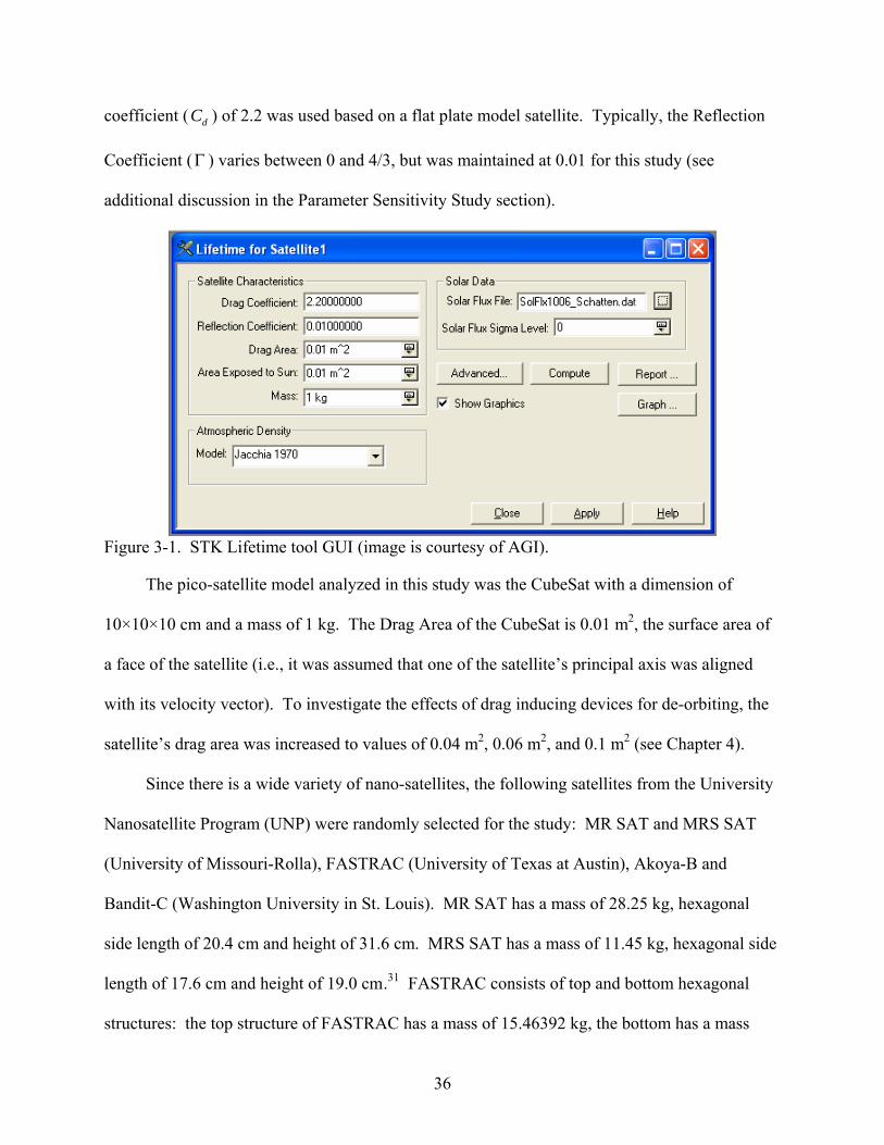
As shown in Figure 3-1, the input for Satellite Characteristics includes Drag Coefficient,

Reflection Coefficient, Drag Area, Area Exposed to Sun, and Mass. For these studies, a drag

36

coefficient ( dC ) of 2.2 was used based on a flat plate model satellite. Typically, the Reflection

Coefficient (Γ ) varies between 0 and 4/3, but was maintained at 0.01 for this study (see

additional discussion in the Parameter Sensitivity Study section).

Figure 3-1. STK Lifetime tool GUI (image is courtesy of AGI).

The pico-satellite model analyzed in this study was the CubeSat with a dimension of

10×10×10 cm and a mass of 1 kg. The Drag Area of the CubeSat is 0.01 m2, the surface area of

a face of the satellite (i.e., it was assumed that one of the satellite’s principal axis was aligned

with its velocity vector). To investigate the effects of drag inducing devices for de-orbiting, the

satellite’s drag area was increased to values of 0.04 m2, 0.06 m2, and 0.1 m2 (see Chapter 4).

Since there is a wide variety of nano-satellites, the following satellites from the University

Nanosatellite Program (UNP) were randomly selected for the study: MR SAT and MRS SAT

(University of Missouri-Rolla), FASTRAC (University of Texas at Austin), Akoya-B and

Bandit-C (Washington University in St. Louis). MR SAT has a mass of 28.25 kg, hexagonal

side length of 20.4 cm and height of 31.6 cm. MRS SAT has a mass of 11.45 kg, hexagonal side

length of 17.6 cm and height of 19.0 cm30F.31 FASTRAC consists of top and bottom hexagonal

structures: the top structure of FASTRAC has a mass of 15.46392 kg, the bottom has a mass

37

12.5757 kg and both are 20.84 cm in height and 47.50 cm in width 31F.32 Akoya-B is a hexagonal

structure that is 45 cm across, 45 cm tall and has a mass of about 25 kg. Bandit-C is a

12×12×18 cm cube with a mass of 2 kg 32F

61.33 The calculated hexagonal surface area of each

satellite was used as the drag area with the exception of Bandit-C, which was calculated as its

length times its width. Each satellite’s mass ( m ), drag area ( A ), area exposed to Sun ( sA ), and

ballistic coefficient are summarized in Table 3-1.

Table 3-1. Satellite mass, drag area, and area exposed to Sun

Satellites Mass (kg) Drag Area* (m2) Area Exposed to Sun* (m2)

Ballistic Coefficient (kg/m2)

CubeSat 1 0.0100 (0.01) 0.0100 (0.01) 45.45 1 0.0400 (0.04) 0.0400 (0.04) 11.36 1 0.0600 (0.06) 0.0600 (0.06) 7.58 1 0.1000 (0.1) 0.1000 (0.1) 4.55 MRS SAT 11.45 0.0805 (0.080478) 0.0805 (0.080478) 65.06 MR SAT 28.25 0.1080 (0.108122) 0.1080 (0.108122) 116.74 FASTRAC

bottom 12.5757 0.1954 (0.195397) 0.1954 (0.195397) 28.59

FASTRAC top 15.4639 0.1954 (0.195397) 0.1954 (0.195397) 35.14 Bandit-C 2 0.0140 (0.0144) 0.0140 (0.0144) 63.13 Akoya-B 25 0.1800 (0.17537) 0.1800 (0.17537) 64.80 *Values of parameters used for analyses are in parenthesis.

Of the ten atmospheric models available in STK, only these seven were used: Jacchia

1970, Jacchia 1971, Jacchia-Roberts, CIRA 1972, MSIS 1986, MSISE 1990, and NRLMSISE

2000. Three other atmospheric models, 1976 Standard, Harris-Priester, and Jacchia 1970

Lifetime, were not used. Based on initial simulations, the 1976 Standard model is only

dependent on altitude and, therefore, shows a single orbital lifetime value. Meanwhile, the

Harris-Priester was found not to agree with the other models according to Woodburn and Lynch

(2005).20 The Jacchia 1970 Lifetime model was retained, in the STK version used for the

analyses, for backward compatibility to previous STK versions 33F.34

The simulations were performed using the solar flux file model SolFlx1006_Schatten.dat,

the most recent file available during the time the simulations were performed. The numbers

38

associated with the flux file names represents the month and year of the data (i.e., 1006

represents October 2006 in this case). Old files are retained for regression analysis. These files

contain predictions of solar radiation flux and geomagnetic index values produced by K. H.

Schatten in ASCII format192H.34 Updated files can be downloaded at “ftp://ftp.agi.com/pub/

DynamicEarthData” and integrated into the software. The solar flux sigma level was maintained

at zero in order to use mean solar flux and weighted planetary geomagnetic index.

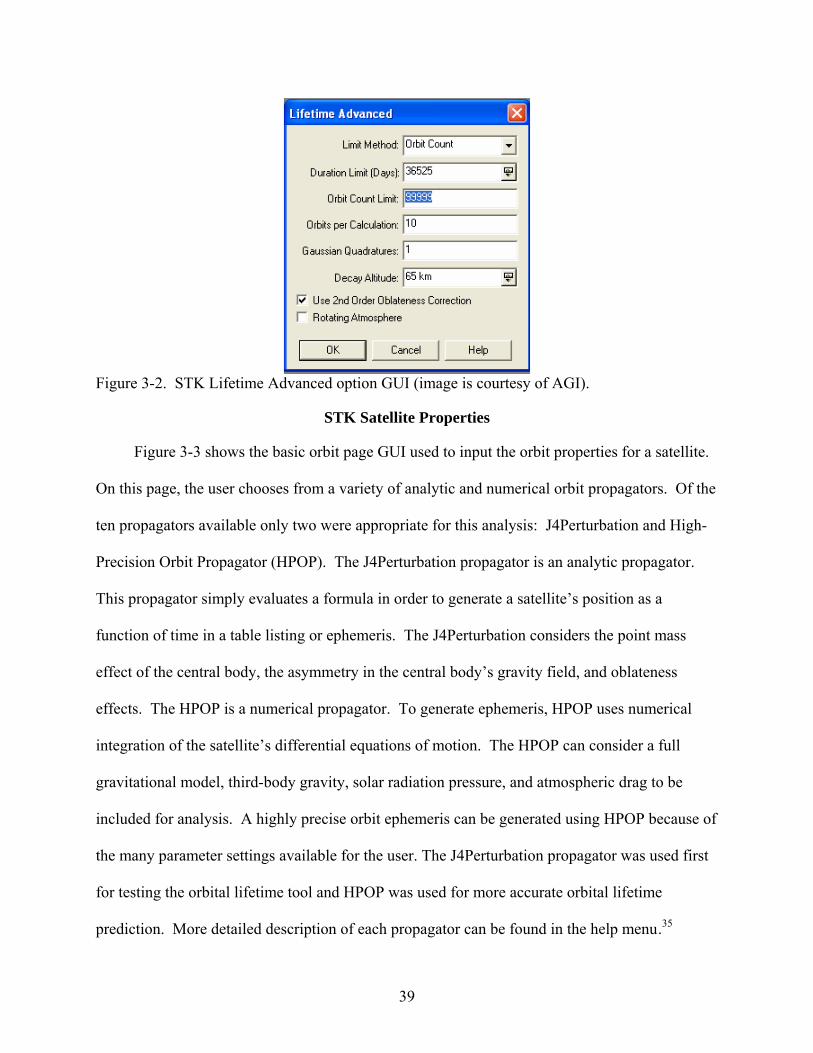
The accuracy and speed of the lifetime calculations are defined by selecting the Advanced

button, which produces the GUI shown in Figure 3-2. The runtime of the lifetime computation

can be limited by the maximum orbit duration (duration), the number of orbit revolutions (orbit

count) or both. The Limit Method was set to Orbit Count in this study. The orbit count limit

was adjusted to a sufficiently large value that allowed the tool to determine the lifetime of the

satellite prior to termination. The number of Orbits per Calculation and the number of Gaussian

Quadratures per orbit used were set at default values to provide a compromise between the

amount of computation time required and the precision of the computation. The Decay Altitude

is the altitude at which calculation of the satellite’s orbit ceases. The default value, 65 km, and a

value of 80 km were used for this research. The default options of a checked 2nd order

oblateness correction and unchecked rotating atmosphere were used. The satellite’s orbital

elements through the duration of its lifetime can be displayed by the report and graph pane.

After calculations are performed the predicted results are displayed in a popup window that

shows a date and time in Gregorian Universal Time Coordinated (UTCG), number of orbits, and

lifetime in days or years down to a tenth of a decimal. It should be emphasized that the results

are estimates due to atmospheric density variations and the difficulty in predicting solar activity

involved with calculating a satellite’s orbital lifetime193H.34

39

Figure 3-2. STK Lifetime Advanced option GUI (image is courtesy of AGI).

STK Satellite Properties

Figure 3-3 shows the basic orbit page GUI used to input the orbit properties for a satellite.

On this page, the user chooses from a variety of analytic and numerical orbit propagators. Of the

ten propagators available only two were appropriate for this analysis: J4Perturbation and High-

Precision Orbit Propagator (HPOP). The J4Perturbation propagator is an analytic propagator.

This propagator simply evaluates a formula in order to generate a satellite’s position as a

function of time in a table listing or ephemeris. The J4Perturbation considers the point mass

effect of the central body, the asymmetry in the central body’s gravity field, and oblateness

effects. The HPOP is a numerical propagator. To generate ephemeris, HPOP uses numerical

integration of the satellite’s differential equations of motion. The HPOP can consider a full

gravitational model, third-body gravity, solar radiation pressure, and atmospheric drag to be

included for analysis. A highly precise orbit ephemeris can be generated using HPOP because of

the many parameter settings available for the user. The J4Perturbation propagator was used first

for testing the orbital lifetime tool and HPOP was used for more accurate orbital lifetime

prediction. More detailed description of each propagator can be found in the help menu34F.35

40

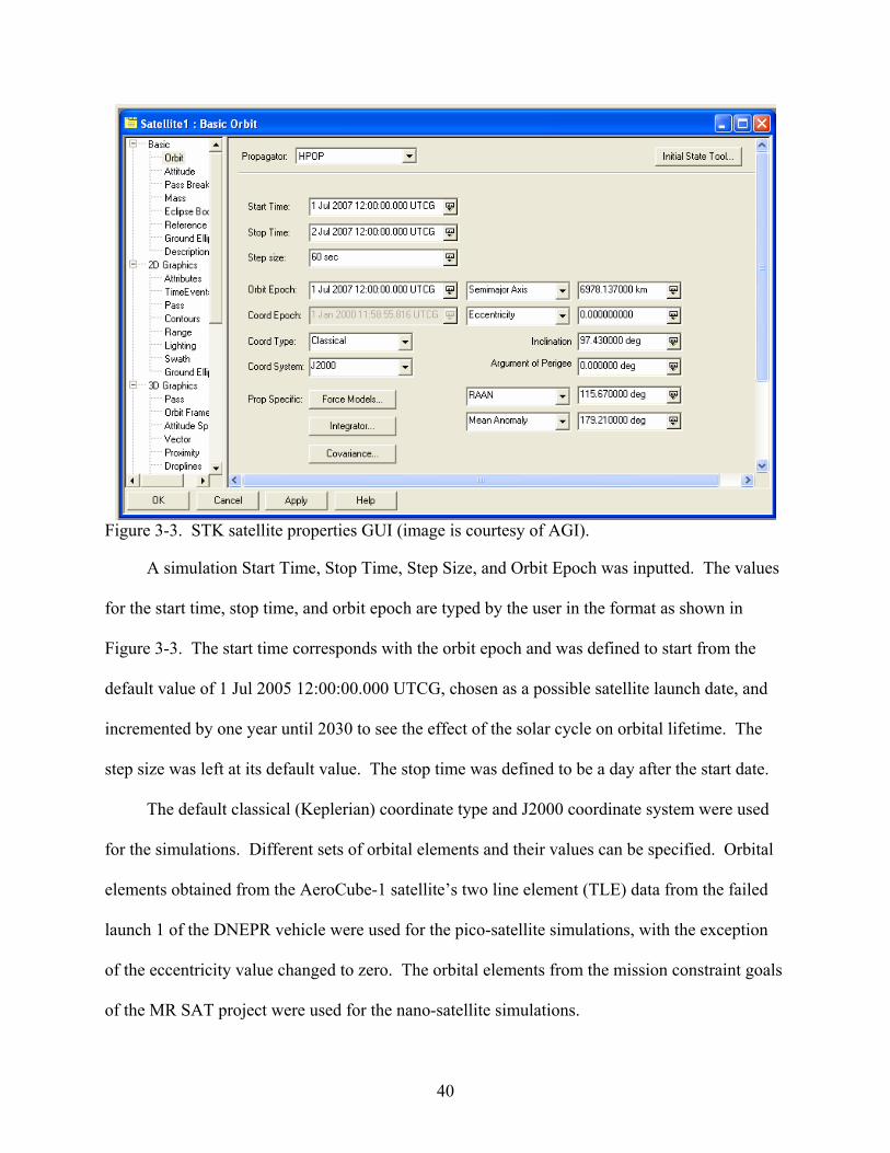
Figure 3-3. STK satellite properties GUI (image is courtesy of AGI).

A simulation Start Time, Stop Time, Step Size, and Orbit Epoch was inputted. The values

for the start time, stop time, and orbit epoch are typed by the user in the format as shown in

Figure 3-3. The start time corresponds with the orbit epoch and was defined to start from the

default value of 1 Jul 2005 12:00:00.000 UTCG, chosen as a possible satellite launch date, and

incremented by one year until 2030 to see the effect of the solar cycle on orbital lifetime. The

step size was left at its default value. The stop time was defined to be a day after the start date.

The default classical (Keplerian) coordinate type and J2000 coordinate system were used

for the simulations. Different sets of orbital elements and their values can be specified. Orbital

elements obtained from the AeroCube-1 satellite’s two line element (TLE) data from the failed

launch 1 of the DNEPR vehicle were used for the pico-satellite simulations, with the exception

of the eccentricity value changed to zero. The orbital elements from the mission constraint goals

of the MR SAT project were used for the nano-satellite simulations.

41

Parameter Sensitivity Study

Simulations were performed varying different parameters such as the reflection coefficient

(Γ ), area exposed to Sun ( sA ), drag coefficient ( dC ), drag area ( A ), and mass ( m ) available

within the lifetime tool to evaluate their effect on orbital lifetime prediction. A summary of the

parameters that were constant for these scenarios is given in Table 3-2. The default epoch of

1 Jul 2005 12:00:00.000 UTCG was chosen as a launch date. The propagator J4Perturbation was

used. The orbital elements obtained from the AeroCube-1 two line element (TLE) were used.

The Jacchia-Roberts atmospheric density model and a decay altitude of 80 km were used.

Table 3-2. Orbital lifetime sensitivity simulation parameters Parameters Figure 3-4 to 3-8 Altitude (km): 550 Epoch Start Date: 1 Jul 2005 12:00:00.000 UTCG Propagator: J4Perturbation Semimajor Axis (km): 6927.248793 Eccentricity: 0.0064 Inclination (deg): 97.43 Argument of Perigee (deg): 189.63 RAAN (deg): 115.67 Mean Anomaly (deg): 349.58 Atmospheric Density Models: Jacchia-Roberts

Two parameters were found not to have significant effect on orbital lifetime, namely the

reflection coefficient (Figure 3-4) and area exposed to Sun (Figure 3-5). As discussed in Chapter

2, these are directly proportional to the acceleration from solar radiation pressure, which was

stated as being less effective than drag below altitudes of 800 km. In this thesis, analyses were

performed at altitudes of 750 km and lower, where such parameters are expected not to affect

orbital lifetime. Consequently, the reflection coefficient was maintained at 0.01, while the area

exposed to Sun value was kept the same as the satellite’s drag area. number of orbits, and

lifetime in days or years with one significant digit after the decimal of the value

Four curves are shown in Figure 3-4 representing drag coefficients of 2.0 (blue-diamond),

42

2.05 (pink-square), 2.1 (green-triangle), and 2.2 (aqua-cross). For each curve, the reflection

coefficient was varied to values of 0, 0.3, 1.0, and 1.8 while the other parameters were kept at a

constant value as seen in the legend. Three curves are shown in Figure 3-5 representing drag

coefficients of 2.0 (blue-diamond), 2.1 (pink-square), and 2.2 (green-triangle). The area exposed

to Sun was varied from 0.05, 0.5, and 1 m2 for each curve. The other parameters were kept at a

constant value as seen in the legend. Both graphs show slopes close to zero, indicating that

orbital lifetime is not affected by the reflection coefficient and the area exposed to Sun.

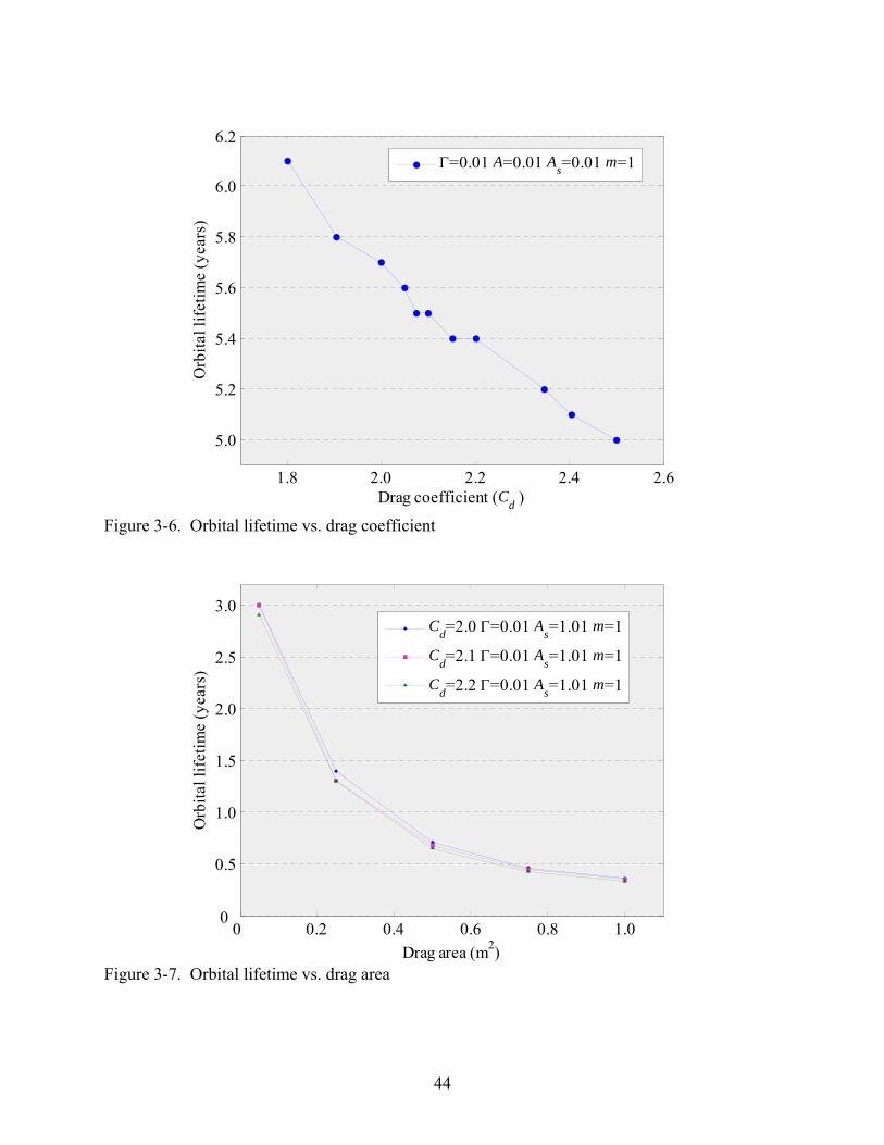
The results from varying the drag coefficient, drag area, and mass are shown in Figures 3-6

to 3-8. Figure 3-6 shows a graph of the orbital lifetime vs. drag coefficient. In this graph, the

drag coefficient was increased to values of 1.8 to 2.5 while the other parameters were kept at

constant values as seen in the legend. Figure 3-7 shows a graph of orbital lifetime vs. drag area.

In this graph, the drag area was increased to values of 0.05 to1 m2. Three curves were obtained

using drag coefficients values of 2.0 (blue-diamond), 2.1 (pink-square), and 2.2 (green-triangle),

while holding the other parameters constant as seen in the legend. All three curves show a

decrease in orbital lifetime. Figure 3-6 shows the dependence of orbital lifetime on the drag

coefficient. Figure 3-7 shows a dependence of orbital lifetime on drag area.

Figure 3-8 shows orbital lifetime vs. mass. In this graph, the value of the mass was

increased to values of 1 to 5 kg while the other parameters were kept at constant values as seen

in the legend. The graph shows an increase in orbital lifetime as a result of the simulation. This

graph shows the dependence of orbital lifetime on mass. The three figures (Figure 3-6 to 3-8)

show the dependence of the orbital lifetime on the three parameters with the given scenario. The

three parameters Cd, A, and m make up the ballistic coefficient, which is expected to affect

orbital lifetime as defined in Chapter 2. For the studies performed in Chapter 4, 0.01 m2 as area

43

exposed to Sun and 0.01 as reflection coefficient value were used because the sensitivity studies

show them to be invariant.

0 0.5 1.0 1.55.1

5.2

5.3

5.4

5.5

5.6

5.7

5.8

Reflection coefficient (Γ)

Orb

ital l

ifetim

e (y

ears

)

Cd=2.0 A=0.01 As=0.01 m=1

Cd=2.05 A=0.01 As=0.01 m=1Cd=2.1 A=0.01 As=0.01 m=1

Cd=2.2 A=0.01 As=0.01 m=1

Figure 3-4. Orbital lifetime vs. reflection coefficient

0 0.2 0.4 0.6 0.8 1.05.2

5.3

5.4

5.5

5.6

5.7

Area exposed to Sun (m2)

Orb

ital l

ifetim

e (y

ears

)

Cd=2.0 Γ=0.01 A=0.01 m=1

Cd=2.1 Γ=0.01 A=0.01 m=1

Cd=2.2 Γ=0.01 A=0.01 m=1

Figure 3-5. Orbital lifetime vs. area exposed to Sun

44

1.8 2.0 2.2 2.4 2.6

5.0

5.2

5.4

5.6

5.8

6.0

6.2

Drag coefficient (Cd )

Orb

ital l

ifetim

e (y

ears

)

Γ=0.01 A=0.01 As=0.01 m=1

Figure 3-6. Orbital lifetime vs. drag coefficient

0 0.2 0.4 0.6 0.8 1.00

0.5

1.0

1.5

2.0

2.5

3.0

Drag area (m2)

Orb

ital l

ifetim

e (y

ears

)

Cd=2.0 Γ=0.01 As=1.01 m=1

Cd=2.1 Γ=0.01 As=1.01 m=1

Cd=2.2 Γ=0.01 As=1.01 m=1

Figure 3-7. Orbital lifetime vs. drag area

45

0 1 2 3 4 5 60

5

10

15

20

25

30

Mass (kg)

Orb

ital l

ifetim

e (y

ears

)

Cd=2.2 Γ=0.01 A=0.01 As=0.01

Figure 3-8. Orbital lifetime vs. mass

46

CHAPTER 4 RESULTS AND DISCUSSION

Simulations of orbital lifetimes for pico- and nano-satellites were performed. The results,

which are presented here, were used to study the effects of different parameters have on their

lifetimes. The CubeSat volume and mass are constant parameters; in order to reduce its lifetime,

the impact of increasing its cross-sectional area was investigated. The volume and mass of the

nano-satellites in this study varied; thus, the impact of different launch altitudes on each nano-

satellites’ lifetime was studied. For both analyses, different launch years were considered to see

the effect of the 11-year solar cycle. Different atmospheric density models were also explored to

determine maximum, minimum, and average orbital lifetime values per launch year.

Pico-satellite Results

Four scenarios were simulated for the CubeSat, with varying drag areas of 0.01, 0.04, 0.06,

and 0.1 m2, which will be referred to as satellite A, B, C, and D, respectively. The CubeSat

simulation parameters are summarized in Table 4-1. An epoch start date of “1 Jul 2007

12:00:00.000 UTCG” was chosen as initial launch date and incremented yearly until 2030 to

determine the effect of the solar cycle, with peaks, known as solar maxima, occurring around

2012 and 2023, and valleys, known as solar minima, at 2007, 2018, and 2029. From 2007 to

2030, a solar cycle is determined from one minimum to the next. These solar maxima and

minima correspond to the years of highest and lowest solar radiation flux values, respectively,

within the solar flux file “SolarFlx1006_Schatten.dat”. The orbital elements for these

simulations closely follow the AeroCube-1 elements, with the exception of changing the

eccentricity to zero. A 600-km initial altitude was used since this value falls within the range at

which the CubeSats would have been released from the DNEPR launch vehicle. Meanwhile, a

decay altitude of 80 km was used for the pico-satellite analyses.

47

Table 4-1. CubeSat simulation parameters Parameters Satellites A and C Satellites B and D Altitude (km): 600 600 Epoch Date: 1 Jul 2007 12:00:00.000 UTCG to

1 Jul 2030 12:00:00.000 UTCG 1 Jul 2007 12:00:00.000 UTCG to 1 Jul 2030 12:00:00.000 UTCG

Propagator: HPOP HPOP Semimajor Axis (km): 6978.137 6978.137 Eccentricity: 0 0 Inclination (deg): 97.43 97.43 Argument of Perigee (deg): 189.63 189.63 RAAN (deg): 115.67 115.67 Mean Anomaly (deg): 349.58 349.58 Drag Coefficient: 2.2 2.2 Reflection Coefficient: 0.01 0.01 Drag Area (m2): 0.01 and 0.06 see figures 0.04 and 0.1 see figures Area Exposed to the Sun (m2): Same as drag area respectively Same as drag area respectively Mass (kg): 1 1 Atmospheric Density Models: Jacchia 1970, Jacchia 1971,

Jacchia-Roberts, CIRA 1972, NRLMSISE 2000, MSISE 1990, MSIS 1986

Jacchia 1970, Jacchia 1971, Jacchia-Roberts

Seven atmospheric density models were used for satellite A (Figure 4-1) and satellite C

(Figure 4-2). The data show trends for certain atmospheric density models, producing maxi-

mum, minimum and average orbital lifetime values per launch year. For the pico-satellites,

orbital lifetimes for four consequent years, starting at 2007, were analyzed for satellites B and D,

using the seven atmospheric density models. From these results, those models that produced

maximum, minimum and close to average orbital lifetime values were determined; these were

then used for the rest of the simulations in order to reduce the analysis time.

The results for satellites A, B, C, and D (Figure 4-3) were plotted using the average life-

time values as a curve, while maximum and minimum orbital lifetime values are shown as error

bars. The orbital lifetime for satellite A ranged from 17 to 27 years, with an average curve value

of 22 years, while that for satellite B is between 2.5 and 9 years, with a mean of 6 years. The

lifetime for satellite C varied from 1 to 8 years, with an average of 4 years, while that for satellite

D were 1 to 5.6 years, with a mean of 3 years. As expected, the orbital lifetimes for satellites B,

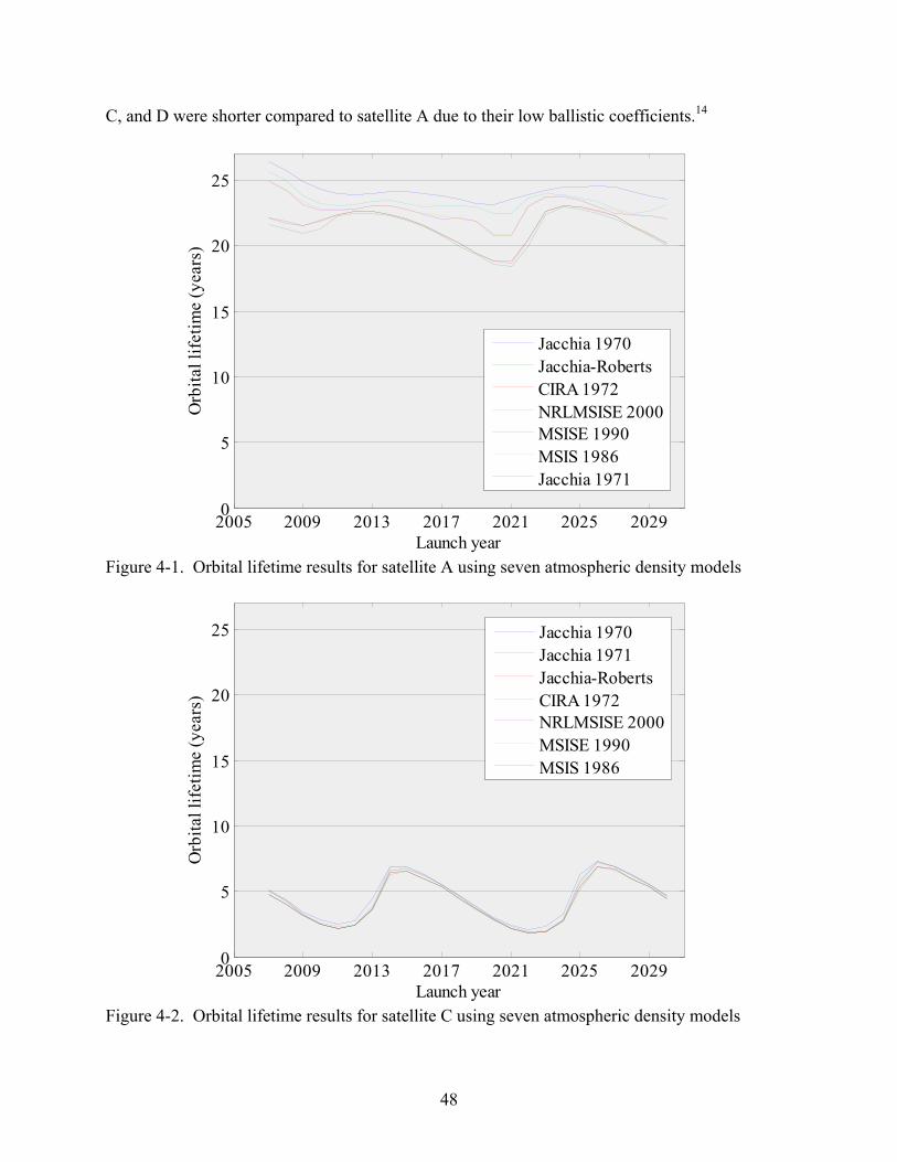
48

C, and D were shorter compared to satellite A due to their low ballistic coefficients.14

2005 2009 2013 2017 2021 2025 20290

5

10

15

20

25

Launch year

Orb

ital l

ifetim

e (y

ears

)

Jacchia 1970Jacchia-RobertsCIRA 1972NRLMSISE 2000MSISE 1990MSIS 1986Jacchia 1971

Figure 4-1. Orbital lifetime results for satellite A using seven atmospheric density models

2005 2009 2013 2017 2021 2025 20290

5

10

15

20

25

Launch year

Orb

ital l

ifetim

e (y

ears

)

Jacchia 1970Jacchia 1971Jacchia-RobertsCIRA 1972NRLMSISE 2000MSISE 1990MSIS 1986

Figure 4-2. Orbital lifetime results for satellite C using seven atmospheric density models

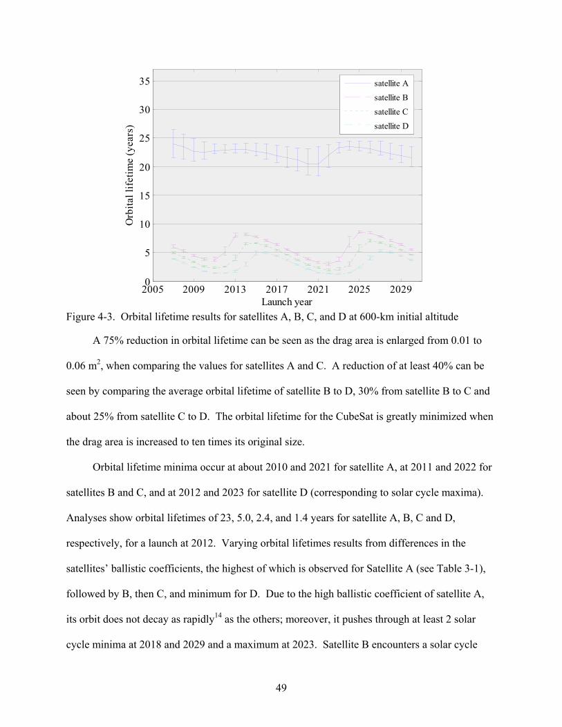
49

2005 2009 2013 2017 2021 2025 20290

5

10

15

20

25

30

35

Launch year

Orb

ital l

ifetim

e (y

ears

)

satellite A

satellite Bsatellite C

satellite D

Figure 4-3. Orbital lifetime results for satellites A, B, C, and D at 600-km initial altitude

A 75% reduction in orbital lifetime can be seen as the drag area is enlarged from 0.01 to

0.06 m2, when comparing the values for satellites A and C. A reduction of at least 40% can be

seen by comparing the average orbital lifetime of satellite B to D, 30% from satellite B to C and

about 25% from satellite C to D. The orbital lifetime for the CubeSat is greatly minimized when

the drag area is increased to ten times its original size.

Orbital lifetime minima occur at about 2010 and 2021 for satellite A, at 2011 and 2022 for

satellites B and C, and at 2012 and 2023 for satellite D (corresponding to solar cycle maxima).

Analyses show orbital lifetimes of 23, 5.0, 2.4, and 1.4 years for satellite A, B, C and D,

respectively, for a launch at 2012. Varying orbital lifetimes results from differences in the

satellites’ ballistic coefficients, the highest of which is observed for Satellite A (see Table 3-1),

followed by B, then C, and minimum for D. Due to the high ballistic coefficient of satellite A,

its orbit does not decay as rapidly14 as the others; moreover, it pushes through at least 2 solar

cycle minima at 2018 and 2029 and a maximum at 2023. Satellite B encounters a solar cycle

50

maximum at 2012 and reenters the atmosphere a year before the next cycle minimum. Satellite

C and D experience a solar maximum only at 2012 and their orbits decays within the following 3

years. The orbits of satellites B, C, and D decay rapidly when launched during a solar maximum

due to their low ballistic coefficients.14

Nano-satellites Results

The nano-satellite simulation parameters are summarized in Table 4-2 for MR SAT and

MRS SAT, Table 4-3 for FASTRAC, and Table 4-4 for Akoya-B and Bandit-C. The epoch start

of “1 Jul 2007 12:00:00.000 UTCG” was chosen as a possible launch date and incremented by a

year until 2030 to see the effect of the solar cycle. For all the simulations, a default decay alti-

tude of 65 km was used. Each satellite’s orbital lifetime was simulated at two different altitudes

and inclination: (1) at 350-km altitude and 51.6º inclination, similar to the orbit of a typical

international space shuttle mission; and, (2) 750-km altitude and 57º inclination, obtained from

the mission constraint goals of the MR SAT project. Atmospheric density models for the simu-

lations were selected by means of the same methods used for satellite B and D. The results were

plotted using the average lifetime values as the curve, and the maximum and minimum values as

error bars.

Simulations were also performed to obtain orbital lifetimes for MR SAT, studying the

effect of different initial altitudes. The parameters used are summarized in Table 4-5. An epoch

start date of “1 Jul 2007 12:00:00.000 UTCG” was chosen as a possible launch date and incre-

mented by yearly until 2030 to see the effect of the solar cycle. The simulation begins at 350-km

initial altitude and is incremented by 50 km until 750 km. An inclination of 51.6º was used.

A decay altitude of 65 km was used. Atmospheric density models used for the simulations were

determined by the same method as for satellite B and D per launch altitude. For each launch

year, the maximum and minimum orbital lifetime values are represented as error bars and the

51

average lifetime values as a curve obtained from the atmospheric density model results. These

values were then used to plot the orbital lifetime versus altitude for MR SAT.

Table 4-2. MR SAT and MRS SAT simulation parameters Parameters Figure 4-4 Figure 4-5 Altitude (km): 350 750 Epoch Date: 1 Jul 2007 12:00:00.000 UTCG to

1 Jul 2030 12:00:00.000 UTCG 1 Jul 2007 12:00:00.000 UTCG to 1 Jul 2030 12:00:00.000 UTCG

Propagator: HPOP HPOP Semimajor Axis (km): 6728.137 7128.137 Eccentricity: 0 0 Inclination (deg): 51.6 57 Argument of Perigee (deg): 0 0 RAAN (deg): 0 0 Mean Anomaly (deg): 0 0 Drag Coefficient: 2.2 2.2 Reflection Coefficient: 0.01 0.01 Drag Area (m2): MR SAT = 0.108122

MRS SAT = 0.080478 MR SAT = 0.108122 MRS SAT = 0.080478

Area Exposed to the Sun (m2): MR SAT = 0.108122 MRS SAT = 0.080478

MR SAT = 0.108122 MRS SAT = 0.080478

Mass (kg): MR SAT = 28.25 MRS SAT = 11.45

MR SAT = 28.25 MRS SAT = 11.45

Atmospheric Density Models: Jacchia-Roberts, CIRA 1972, NRLMSISE 2000

Jacchia 1970, Jacchia-Roberts, MSIS 1986

Table 4-3. FASTRAC simulation parameters Parameters Figure 4-6 Figure 4-7 Altitude (km): 350 750 Epoch Date: 1 Jul 2007 12:00:00.000 UTCG to

1 Jul 2030 12:00:00.000 UTCG 1 Jul 2007 12:00:00.000 UTCG to 1 Jul 2030 12:00:00.000 UTCG

Propagator: HPOP HPOP Semimajor Axis (km): 6728.137 7128.137 Eccentricity: 0 0 Inclination (deg): 51.6 57 Argument of Perigee (deg): 0 0 RAAN (deg): 0 0 Mean Anomaly (deg): 0 0 Drag Coefficient: 2.2 2.2 Reflection Coefficient: 0.01 0.01 Drag Area (m2): top = 0.195397

bottom = 0.193597 top = 0.195397 bottom = 0.193597

Area Exposed to the Sun (m2): top = 0.195397 bottom = 0.193597

top = 0.195397 bottom = 0.193597

Mass (kg): top = 15.4639 bottom = 12.5757

top = 15.4639 bottom = 12.5757

Atmospheric Density Models: Jacchia-Roberts, CIRA 1972, NRLMSISE 2000

Jacchia 1970, Jacchia-Roberts, NRLMSISE 2000, MSIS 1986

52

Table 4-4. Akoya-B and Bandit-C simulation parameters Parameters Figure 4-8 Figure 4-9 Altitude (km): 350 750 Epoch Date: 1 Jul 2007 12:00:00.000 UTCG to

1 Jul 2030 12:00:00.000 UTCG 1 Jul 2007 12:00:00.000 UTCG to 1 Jul 2030 12:00:00.000 UTCG

Propagator: HPOP HPOP Semimajor Axis (km): 6728.137 7128.137 Eccentricity: 0 0 Inclination (deg): 51.6 57 Argument of Perigee (deg): 0 0 RAAN (deg): 0 0 Mean Anomaly (deg): 0 0 Drag Coefficient: 2.2 2.2 Reflection Coefficient: 0.01 0.01 Drag Area (m2): Akoya-B = 0.17537

Bandit-C = 0.0144 Akoya-B = 0.17537 Bandit-C = 0.0144

Area Exposed to the Sun (m2): Akoya-B = 0.17537 Bandit-C = 0.0144

Akoya-B = 0.17537 Bandit-C = 0.0144

Mass (kg): Akoya-B = 25 Bandit-C = 2

Akoya-B = 25 Bandit-C = 2

Atmospheric Density Models: Jacchia-Roberts, CIRA 1972, NRLMSISE 2000

Jacchia 1970, Jacchia-Roberts, MSIS 1986

Table 4-5. MR SAT with different initial altitudes simulation parameters Parameters Figure 4-10 Altitude (km): 350 to 750 Epoch Date: 1 Jul 2007 12:00:00.000 UTCG to

1 Jul 2030 12:00:00.000 UTCG Propagator: HPOP Semimajor Axis (km): 6728.137 to 7128.137 Eccentricity: 0 Inclination (deg): 51.6 Argument of Perigee (deg): 0 RAAN (deg): 0 Mean Anomaly (deg): 0 Drag Coefficient: 2.2 Reflection Coefficient: 0.01 Drag Area (m2): 0.108122 Area Exposed to the Sun (m2): 0.108122 Mass (kg): 28.25 Atmospheric Density Models: Jacchia 1970, Jacchia 1971, Jacchia-Roberts, CIRA

1972, NRLMSISE 2000, MSISE 1990, MSIS 1986

The results for MR SAT and MRS SAT (Figure 4-4), with an initial altitude of 350 km,

show orbital lifetime values between 140 and 370 days for the former, with an average curve

value of 247 days, and between 80 and 210 days for the latter, with an average curve of

53

141 days. Orbital lifetime minima for the average curves in Figure 4-4 occur at 2012 and 2023

for both satellites. On the other hand, the results at 750-km initial altitude (Figure 4-5) show

orbital lifetime values between 460 and 540 years for MR SAT, with an average curve value of

495 years, and between 250 and 300 years for MRS SAT, with an average curve value of

269 years. The lifetime minima for the average curve in Figure 4-5 occur at 2011 and 2021 for

MR SAT, and at 2011 and 2020 for MRS SAT.

At an initial altitude of 350 km, the results for the FASTRAC top and the bottom satellites

(Figure 4-6), show orbital lifetime values for FASTRAC top is between 50 and 125 days, with an

average curve value of 86 days, and from 40 to 110 days for the bottom, with an average curve

value of 72 days. Orbital lifetime minima for the average curves in Figure 4-6 occur at 2012 and

2023 for both satellites. On the other hand, results at 750-km initial altitude (Figure

4-7) show orbital lifetime values between 140 and 165 years, with an average curve value of

151 years for the top satellite, and from 110 to 135 years for the bottom satellite, with an average

curve value of 122 years. Orbital lifetime minima for the average curves in Figure 4-7 occur at

about 2011 and 2021 for the top satellite and at about 2010 and 2020 for the bottom satellite.

The results for Akoya-B and Bandit-C at an initial altitude of 350 km (Figure 4-8) show

orbital lifetime values between 86 and 210 days with an average curve value of 141 days for both

satellites. Orbital lifetime minima for the average curves in Figure 4-8 occur at 2012 and 2023

for both satellites. Meanwhile, the results at 750-km initial altitude (Figure 4-9) show orbital

lifetime values between 255 and 295 years for Akoya-B, with average curve value 270 years, and

from 250 to 285 years for Bandit-C, with an average curve value of 263 years. Orbital lifetime

minima for the average curves in Figure 4-9 occur at 2011 and 2022 for Akoya-B, and at about

2010 and 2021 for Bandit-C.

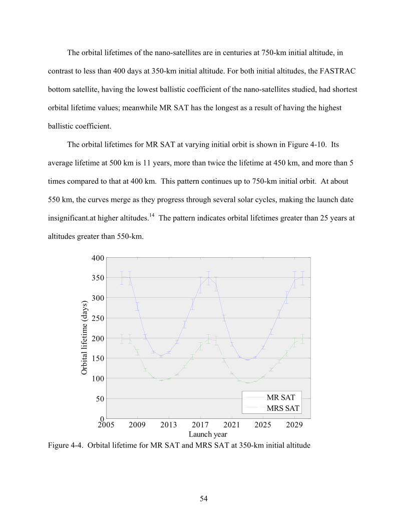
54

The orbital lifetimes of the nano-satellites are in centuries at 750-km initial altitude, in

contrast to less than 400 days at 350-km initial altitude. For both initial altitudes, the FASTRAC

bottom satellite, having the lowest ballistic coefficient of the nano-satellites studied, had shortest

orbital lifetime values; meanwhile MR SAT has the longest as a result of having the highest

ballistic coefficient.

The orbital lifetimes for MR SAT at varying initial orbit is shown in Figure 4-10. Its

average lifetime at 500 km is 11 years, more than twice the lifetime at 450 km, and more than 5

times compared to that at 400 km. This pattern continues up to 750-km initial orbit. At about

550 km, the curves merge as they progress through several solar cycles, making the launch date

insignificant.at higher altitudes.14 The pattern indicates orbital lifetimes greater than 25 years at

altitudes greater than 550-km.

2005 2009 2013 2017 2021 2025 20290

50

100

150

200

250

300

350

400

Launch year

Orb

ital l

ifetim

e (d

ays)

MR SATMRS SAT

Figure 4-4. Orbital lifetime for MR SAT and MRS SAT at 350-km initial altitude

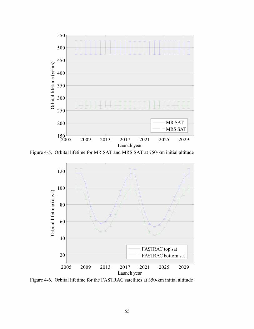
55

2005 2009 2013 2017 2021 2025 2029150

200

250

300

350

400

450

500

550

Launch year

Orb

ital l

ifetim

e (y

ears

)

MR SATMRS SAT

Figure 4-5. Orbital lifetime for MR SAT and MRS SAT at 750-km initial altitude

2005 2009 2013 2017 2021 2025 2029

20

40

60

80

100

120

Launch year

Orb

ital l

ifetim

e (d

ays)

FASTRAC top satFASTRAC bottom sat

Figure 4-6. Orbital lifetime for the FASTRAC satellites at 350-km initial altitude

56

2005 2009 2013 2017 2021 2025 202990

100

110

120

130

140

150

160

170

Launch year

Orb

ital l

ifetim

e (y

ears

)

FASTRAC top satFASTRAC bottom sat

Figure 4-7. Orbital lifetime for the FASTRAC satellites at 750-km initial altitude

2005 2009 2013 2017 2021 2025 202940

60

80

100

120

140

160

180

200

Launch year

Orb

ital l

ifetim

e (d

ays)

Akoya-BBandit-C

Figure 4-8. Orbital lifetime for the Akoya-B and Bandit-C at 350-km initial altitude

57

2005 2009 2013 2017 2021 2025 2029230

240

250

260

270

280

290

300

Launch year

Orb

ital l

ifetim

e (y

ears

)

Akoya-BBandit-C

Figure 4-9. Orbital lifetime for the Akoya-B and Bandit-C at 750-km initial altitude

300 400 500 600 700 80010

-1

100

101

102

103

Altitude (km)

Orb

ital l

ifetim

e (y

ears

)

Figure 4-10. Orbital lifetime for the MR SAT using different initial altitudes

58

CHAPTER 5 CONCLUSION AND RECOMMENDATIONS

Conclusions

Lifetime analyses of pico- and nano-satellites were conducted using the Satellite Tool Kit

(STK) orbital Lifetime tool. The pico-satellite analyses were performed on the standard CubeSat

developed by CalPoly and Stanford, whereas the nano-satellite analyses were performed on three

randomly selected satellites from the University Nano-satellite Program (UNP). Typical mission

scenarios for these two classes of satellites were investigated. Since the prediction of orbital

lifetime is not an exact science, parameters which have an effect on the prediction were varied to

provide ranges of expected lifetimes for the different scenarios.

The results indicate that orbital lifetimes of pico-satellites can be significantly reduced by

increasing their drag area from 0.01, to 0.04, 0.06 or 0.1 m2. The longest that the CubeSat is

predicted to stay up in orbit at a 600 km altitude with a drag area of 0.01 m2 is approximately 27

years, which is slightly above the FCC debris mitigation guidelines. The longest that the

CubeSat is predicted to stay in orbit at a 600 km altitude with a drag area of 0.04 m2 is about 8.8

years, 0.06 m2 is about 7 years, and 0.1 m2 about 5.5 years. Changing the drag area of a 1-kg

satellite from 0.01 to 0.1 m2 decreased its orbital lifetime from an average of 22 to 3 years and

results in 86% reduction. The results show that changing the drag areas to 0.04 or 0.1 m2 did not

make a significant difference to the reduced total amount of lifetime of the satellite than the drag

area of 0.06 m2. At 600 km above the Earth’s surface, a pico-satellite with drag area of 0.1 m2

had minimum orbital lifetimes during years of highest solar activity due to its low ballistic

coefficient. At this same altitude, pico-satellites with smaller drag areas, which results in higher

ballistic coefficient, responded more slowly to the solar activity and as a result the orbital

lifetime minimums appear shifted from solar maximum years. This analysis implies that passive

59

de-orbiting devices such as drag chutes can be effective devices for addressing orbital debris

mitigation. The analyses also imply that in order to obtain minimum orbital lifetimes to set the

launch year of the satellite corresponding with high solar activity that is at solar maximum.

The nano-satellites used in this study were between 11 to 28 kg, with drag areas from 0.08

and 0.2 m2. The results of the nano-satellites analyses, with a launch altitude of 350 km, show

that the orbital lifetimes are in number of days. At this altitude the satellites will reenter the

atmosphere in a short amount of time. These lifetime values will meet the FCC mitigation

guidelines. The results of the nano-satellites analyses, with an altitude of 750 km, show that the

orbital lifetimes are in centuries. At this high altitude the nano-satellites’ orbital lifetime will not

meet the FCC mitigation guidelines. Values indicate that additions to the nano-satellites are

needed to fulfill the 25 year orbital lifetime requirements at this altitude. The nano-satellites in

high orbit, above 500 km, have a problem of potentially becoming a debris space. The nano-

satellites do not have a volume or mass requirement as the CubeSats, therefore these were kept

constant respectively per satellite and only the effect of a change in altitude on their orbital

lifetimes were investigated.

Recommendations

There are different parameters to consider with prediction of long-term orbital lifetime and

its reduction. Satellites properties (i.e., geometry, mass and the solar activity, have significant

effects on these. For mission operations the implementation of an aerobraking technique for

both CubeSats and nano-satellites, that is a change in their drag area, should be further

investigated. For mission planning the consideration of proposed satellites to be launched during

the solar maximum time period should be further investigated.

60

LIST OF REFERENCES

1.National Research Council (U.S) Committee on Space Debris, “Orbital Debris: A Technical Assessment,” National Academy Press, Washington, DC, 1995, Chaps. 4, 8.

2.“NASA Safety Standard: Guidelines and Assessment Procedures for Limiting Orbital Debris,” NSS 1740.14, August 1995.

3.Flury, W., “Space Debris,” Preparing for the Future [online], Vol. 4, No. 4, 1994, http://esapub.esrin.esa.it/pff/pffv4n4/ppfflunr4.htm [retrieved 26 June 2007].

4.Aerospace Corporation, Center for Orbital and Reentry Debris Studies, “Space Debris Basics: What is the Future Trend?,” http://www.aero.org/capabilities/cords/debris-future.html [accessed 26 June 2007].

5.Walker, S. H., ““Responsive” Access and Infrastructure,” Proceedings of DarpaTech 2005, Defense Advance Research Project Agency (DARPA), Anaheim, CA, August 2005, pp. 203-207.

6.Calpoly, CubeSat, “Mission Statement”, http://cubesat.atl.calpoly.edu/ pages/home/mission-statement.php [accessed on 30 June 2007].

7.AFOSR, AFRL Space Vehicles, AIAA, NASA, SMC Det 12, “About the University Nanosatellite Program,” http://www.vs.afrl.af.mil/UNP/About.html [accessed on 19 July 2007].

8.Orbital Debris Program Office, NASA Johnson Space Center, “Orbital Debris Education Package,” http://www.orbitaldebris.jsc.nasa.gov/library/EducationPackage.pdf [retrieved 11 July 2007].

9.“Technical Report On Space Debris,” United Nations, (A/AC.105/720), New York, 1999.

10. Orbital Debris Program Office, NASA Johnson Space Center, “Orbital Debris Mitigation,” http://www.orbitaldebris.jsc.nasa.gov/mitigate/mitigation.html [accessed 27 June 2007].

11. “U.S. Government Begins Orbital Debris Meetings with Industry,” The Orbital Debris Quarterly News, Vol. 4, No. 4, 1999, p. 4.

12. “U. S. Government Orbital Debris Mitigation Standard Practices” at the Johnson Space Center [online], 1997, http://www.orbitaldebris.jsc.nasa.gov/library/ USG_OD_Standard_Practices.pdf [accessed 1 July 2007].

13. “In the Matter of Mitigation of Orbital Debris,” Federal Communications Commission, FCC 04-130, Washington, DC, June 2004, p. 2.

14. Wertz, J. R., and Larson, W. J., Space Mission Analysis and Design, 3rd ed., Microcosm Press, Torrence, CA, 1999, Chaps. 5, 6, 8.

61

15. “IADC Space Debris Mitigation Guidelines,” Inter-Agency Space Debris Coordination Committee, IADC-02-01, October 2002.

16. Calpoly, CubeSat, “Dnepr Launch Vehicle Status - Integrated for Launch”, http://cubesat.atl.calpoly.edu/pages/missions/dnepr-launch-2/satellite-status.php [accessed 30 June 2007].

17. AMSAT, “Cubesat Information,” http://www.amsat.org/amsat-new/satellites/cubesats.php [accessed 27 June 2007].

18. Orbital Debris Program Office, NASA Johnson Space Center, “Orbital Debris Graphics,” http://www.orbitaldebris.jsc.nasa.gov/photogallery/beehives.html#leo [accessed 27 June 2007].

19. Bate, R. R., Mueller, D. D., and White, J. R., “Two-body Orbital Mechanics,” Fundamentals of Astrodynamics, Dover Publications, Inc., New York, 1971, Chap. 1.

20. Woodburn, J., and Lynch, S., “A Numerical Study of Orbital Lifetime (revised),” Proceedings of the 2005 AAS/AIAA Astrodynamics Specialists Conference, Paper No. AAS 05-297, Lake Tahoe, CA, August 2005.

21. De Lafontaine, J., and Garg, S. C., “A review of satellite lifetime and orbit decay prediction,” Proc. Indian Acad. Sci. (Engg. Sci.), Vol. 5, Pt. 3, September 1982, pp. 197-258.

22. Ladner, J. E., and Ragsdale, G. C., “Earth Orbital Satellite Lifetime,” NASA TN D-1995, January 1964.

23. Vallado, D. A., “Special Perturbation Techniques,” Fundamentals of Astrodynamics and Applications, 2nd ed., Microcosm Press, El Segundo, CA, 2001, Chap. 8.

24. Orr, L.H., “User’s Guide for Langley Research Center Orbital Lifetime Program,” NASA TM-87587, September 1985.

25. Battin, R. H., “Variation of Parameters,” An Introduction to the Mathematics and Methods of Astrodynamics, Revised Edition, Revised ed., American Institute of Aeronautics and Astronautics, Inc., Reston, VA, 1999, Chap. 10.

26. Belcher, S. J., Rowell, L. N., and Smith, M. C., “Satellite Lifetime Program,” The Rand Corporation, RM-4007-NASA, April 1964.

27. Space Mission Analysis and Design, “SatLife Stand-Alone Module v1.0,” http://www.smad.com/software/agimo3.html [accessed 21 May 2007].

28. Alan Pickup, “Satellite tracking and decay information,” http://www.wingar.demon.co.uk/ satevo [accessed 21 June 2007].

29. Analytical Graphics, Inc., “About AGI,” http://www.agi.com/corporate [accessed 27 June 2007].

62

30. Analytical Graphics, Inc., “STK Editions,” http://www.agi.com/products/desktopApp/ stkFamily/editions/index.cfm?tab=key [accessed 27 June 2007].

31. University of Missouri-Rolla, “Conceptual Design of the MR SAT Tethered Satellite Project at the University of Missouri-Rolla: 1.0 Structures,” http://web.umr.edu/~mrsat/docs.html [accessed 12 February 2007].

32. Holt, G., Stewart, S., Mauldin, J., Campbell, T., Eckhoff, P., Yeldell, S., Greenbaum, J., Linford, M., Diaz-Aguado, M., Wang, T., Berthold, T., Lightsey, E. G., Raja, L. L., Ebinuma, T., “FASTRAC Mission Plan: Formation Autonomy Spacecraft with Thrust, Rel-Nav, Attitude and Crosslink,” The University of Texas at Austin, Austin, TX, December 2005.

33. Washington University, “Welcome to the Washington University Nanosat Page,” http://www.me.wustl.edu/faculty/mas/nanosat [accessed 12 February 2007].

34. Analytical Graphics, Inc., “Lifetime Tool,” http://www.agi.com/resources/ help/stk613/helpSystem/stk/tools-11.htm [accessed 1 July 2007].

35. Analytical Graphics, Inc., “Satellite Orbits,” http://www.agi.com/resources/ help/stk613/helpSystem/stk/vehSat_orbitTab.htm [accessed 1 July 2007].

63

BIOGRAPHICAL SKETCH

The author was born in Quezon City, Philippines. She immigrated to the United States in

Illinois on October 15, 1988. She received her bachelor’s degree in Electrical Engineering on

December 2002 from the University of Illinois at Chicago. In August 2007, she moved to

Florida to attend the University of Florida in Gainesville. She received her master’s degree in

Mechanical Engineering in December 2007 with a concentration in dynamics and control.