Big Data for Oracle Devs - Towards Spark, Real-Time and Predictive Analytics

Oracle® Retail Predictive Application Server
User Guide Release 12.1.2
November 2007

Oracle® Retail Predictive Application Server User Guide, Release 12.1.2
Copyright © 2007, Oracle. All rights reserved.
Primary Author: Melody Crowley
The Programs (which include both the software and documentation) contain proprietary information; they are provided under a license agreement containing restrictions on use and disclosure and are also protected by copyright, patent, and other intellectual and industrial property laws. Reverse engineering, disassembly, or decompilation of the Programs, except to the extent required to obtain interoperability with other independently created software or as specified by law, is prohibited.
The information contained in this document is subject to change without notice. If you find any problems in the documentation, please report them to us in writing. This document is not warranted to be error-free. Except as may be expressly permitted in your license agreement for these Programs, no part of these Programs may be reproduced or transmitted in any form or by any means, electronic or mechanical, for any purpose.
If the Programs are delivered to the United States Government or anyone licensing or using the Programs on behalf of the United States Government, the following notice is applicable:
U.S. GOVERNMENT RIGHTS Programs, software, databases, and related documentation and technical data delivered to U.S. Government customers are "commercial computer software" or "commercial technical data" pursuant to the applicable Federal Acquisition Regulation and agency-specific supplemental regulations. As such, use, duplication, disclosure, modification, and adaptation of the Programs, including documentation and technical data, shall be subject to the licensing restrictions set forth in the applicable Oracle license agreement, and, to the extent applicable, the additional rights set forth in FAR 52.227-19, Commercial Computer Software—Restricted Rights (June 1987). Oracle Corporation, 500 Oracle Parkway, Redwood City, CA 94065
The Programs are not intended for use in any nuclear, aviation, mass transit, medical, or other inherently dangerous applications. It shall be the licensee's responsibility to take all appropriate fail-safe, backup, redundancy and other measures to ensure the safe use of such applications if the Programs are used for such purposes, and we disclaim liability for any damages caused by such use of the Programs.
Oracle, JD Edwards, PeopleSoft, and Siebel are registered trademarks of Oracle Corporation and/or its affiliates. Other names may be trademarks of their respective owners.
The Programs may provide links to Web sites and access to content, products, and services from third parties. Oracle is not responsible for the availability of, or any content provided on, third-party Web sites. You bear all risks associated with the use of such content. If you choose to purchase any products or services from a third party, the relationship is directly between you and the third party. Oracle is not responsible for: (a) the quality of third-party products or services; or (b) fulfilling any of the terms of the agreement with the third party, including delivery of products or services and warranty obligations related to purchased products or services. Oracle is not responsible for any loss or damage of any sort that you may incur from dealing with any third party.

iii
Value-Added Reseller (VAR) Language (i) the software component known as ACUMATE developed and licensed by Lucent Technologies Inc. of Murray Hill, New Jersey, to Oracle and imbedded in the Oracle Retail Predictive Application Server – Enterprise Engine, Oracle Retail Category Management, Oracle Retail Item Planning, Oracle Retail Merchandise Financial Planning, Oracle Retail Advanced Inventory Planning and Oracle Retail Demand Forecasting applications.
(ii) the MicroStrategy Components developed and licensed by MicroStrategy Services Corporation (MicroStrategy) of McLean, Virginia to Oracle and imbedded in the MicroStrategy for Oracle Retail Data Warehouse and MicroStrategy for Oracle Retail Planning & Optimization applications.
(iii) the SeeBeyond component developed and licensed by Sun MicroSystems, Inc. (Sun) of Santa Clara, California, to Oracle and imbedded in the Oracle Retail Integration Bus application.
(iv) the Wavelink component developed and licensed by Wavelink Corporation (Wavelink) of Kirkland, Washington, to Oracle and imbedded in Oracle Retail Store Inventory Management.
(v) the software component known as Crystal Enterprise Professional and/or Crystal Reports Professional licensed by Business Objects Software Limited (“Business Objects”) and imbedded in Oracle Retail Store Inventory Management.
(vi) the software component known as Access Via™ licensed by Access Via of Seattle, Washington, and imbedded in Oracle Retail Signs and Oracle Retail Labels and Tags.
(vii) the software component known as Adobe Flex™ licensed by Adobe Systems Incorporated of San Jose, California, and imbedded in Oracle Retail Promotion Planning & Optimization application.
(viii) the software component known as Style Report™ developed and licensed by InetSoft Technology Corp. of Piscataway, New Jersey, to Oracle and imbedded in the Oracle Retail Value Chain Collaboration application.
(ix) the software component known as i-net Crystal-Clear™ developed and licensed by I-NET Software Inc. of Berlin, Germany, to Oracle and imbedded in the Oracle Retail Central Office and Oracle Retail Back Office applications.
(x) the software component known as WebLogic™ developed and licensed by BEA Systems, Inc. of San Jose, California, to Oracle and imbedded in the Oracle Retail Value Chain Collaboration application.
(xi) the software component known as DataBeacon™ developed and licensed by Cognos Incorporated of Ottawa, Ontario, Canada, to Oracle and imbedded in the Oracle Retail Value Chain Collaboration application.


v
Contents Preface .............................................................................................................................. xi
Audience ...................................................................................................................................xi Related Documents ...................................................................................................................xi Customer Support .....................................................................................................................xi Review Patch Documentation...................................................................................................xi Oracle Retail Documentation on the Oracle Technology Network...........................................xi Conventions ............................................................................................................................ xii
1 Introduction .................................................................................................................... 1 Overview....................................................................................................................................1
More Information................................................................................................................1 Getting Started ...........................................................................................................................2
Logging on to Oracle Retail Predictive Solutions ..............................................................2 Changing Your Password ...................................................................................................4 Logging Off and Leaving the Login Information Screen Open..........................................4 Logging Off and Exiting the System ..................................................................................5
2 Basic RPAS Concepts ................................................................................................... 7 Multidimensional Databases ......................................................................................................7
Relational Databases...........................................................................................................7 Two-Dimensional Data Array ............................................................................................7 Dimensions .........................................................................................................................8 Three-Dimensional Relational Table..................................................................................9 Four-Dimensional Data Array ..........................................................................................10
Hierarchies ...............................................................................................................................10 Hierarchy Rules ................................................................................................................11
Workbooks, Worksheets, and Wizards ....................................................................................12 Workbooks........................................................................................................................12 Worksheets .......................................................................................................................12 Wizards.............................................................................................................................13
Menus, Quick Menus, and Toolbars ........................................................................................13 Menus ...............................................................................................................................13 Quick Menus.....................................................................................................................13 Toolbars ............................................................................................................................13
3 Using Workbooks, Worksheets, and Wizards........................................................... 15 Using Workbooks and Worksheets..........................................................................................15
Overview ..........................................................................................................................15 Menu Bar ..........................................................................................................................15 The New Dialog Box ........................................................................................................26
Workbook and Worksheet Components ..................................................................................33 Overview ..........................................................................................................................33 Status Bar..........................................................................................................................34 Hierarchy Tiles and Display Area.....................................................................................34
Workbook and Worksheet Procedures.....................................................................................36 Basic Workbook Procedures.............................................................................................36 Save and Delete Workbook Formats ................................................................................38 Manage Multiple Workbook Windows ............................................................................39 Print Worksheets and Generate Reports ...........................................................................40 Commit Changes to the Master Database .........................................................................48 Working with Cells...........................................................................................................49 Cut, Copy, and Paste Base-Level Data .............................................................................52 Cut, Copy, and Paste Multiple Slices................................................................................54 Copy Data to and Paste Data from the Windows Clipboard1...........................................55
vi
Enlarge and Zoom on the Screen ......................................................................................56 Change the View of Your Display....................................................................................56 Change Charts to Grids and Back.....................................................................................57 Show and Hide the Button Text, Status Bar, and Toolbar ................................................57 Enter Measure Data Using a Scaling Factor .....................................................................58 Locate Items in the Worksheet .........................................................................................59 Rotate or Pivot an Axis on a Grid.....................................................................................60 Show and Hide Positions in the Grid Display...................................................................60 Show and Hide Positions in the Measure Hierarchy.........................................................61 Measure Profiles ...............................................................................................................62 Select a Higher Hierarchy Level for Data Roll-Up...........................................................64 Aggregate Data .................................................................................................................64 Dimension and Sorting Attributes ....................................................................................66 Dimension Splitting ..........................................................................................................78 Dynamic Position Maintenance (Dynamic Add) ..............................................................81 Lock and Unlock Cells and Measures ..............................................................................89 Change the Format of a Grid ............................................................................................93 Format Grid Components .................................................................................................96 Format the Display of Grid Lines .....................................................................................96 Change the Format of a Measure ......................................................................................98 Specify Options for Deferred Calculations.....................................................................100 Specify Type-Based Formatting Options for Measures..................................................105 Create and Format Charts ...............................................................................................107 Change Data Values within a Chart................................................................................113
Using Wizards........................................................................................................................115 Wizards...........................................................................................................................115 Wizard Procedures..........................................................................................................116
4 Changing Views of Data in Worksheets .................................................................. 121 Aggregation ...........................................................................................................................121
Overview ........................................................................................................................121 Data Aggregation in a Worksheet...................................................................................122 Display Worksheet Data in Chart Form..........................................................................124
Pivoting Data .........................................................................................................................125 Rotating Data .........................................................................................................................126
Reposition a Hierarchy Tile............................................................................................126 Cursor Indicators when Rotating Data............................................................................127
Selecting Items.......................................................................................................................127 Selecting Items in a Wizard List.....................................................................................128 Selecting Items in the Grid .............................................................................................128
Spreading ...............................................................................................................................128 Spreading Aggregate Forecast Values ............................................................................129 REPD Functionality........................................................................................................129
Worksheet Axis......................................................................................................................130 5 Using Special RPAS Features .................................................................................. 133
Exception Management and Alerts ........................................................................................133 Overview ........................................................................................................................133 Using the Alert Manager.................................................................................................133
Percent-of-Parent Measures ...................................................................................................141 Overview ........................................................................................................................141 Definition and Usage ......................................................................................................141 Absolute..........................................................................................................................142 Relative...........................................................................................................................142
A Appendix: Using RPAS Menus and Toolbars......................................................... 145 Application Main Menu Bar ..................................................................................................145
vii
Menu Shortcuts...............................................................................................................145 File Menu...............................................................................................................................145
File – Change Password..................................................................................................145 File – New ......................................................................................................................145 File – Open .....................................................................................................................145 File – Save ......................................................................................................................145 File – Save As.................................................................................................................146 File – Close.....................................................................................................................146 File – Delete....................................................................................................................147 File – Exit .......................................................................................................................147 File – Logoff ...................................................................................................................147 File – Commit Status ......................................................................................................147 File – Commit ASAP......................................................................................................147 File – Export Sheet .........................................................................................................147 File – MRU (Most Recently Used) List..........................................................................148 File – Page Setup ............................................................................................................148 File – Print ......................................................................................................................149 File – Print Multiple........................................................................................................149 File – Print Preview ........................................................................................................149 File – Refresh..................................................................................................................150
Edit Menu ..............................................................................................................................150 Edit – Cut........................................................................................................................150 Edit – Cut Special ...........................................................................................................150 Edit – Copy.....................................................................................................................152 Edit – Copy Special ........................................................................................................152 Edit – Paste .....................................................................................................................153 Edit – Paste Special ........................................................................................................154 Edit – Paste from Clipboard............................................................................................157 Edit – Revert ...................................................................................................................157 Edit – Fill ........................................................................................................................158 Edit – Clear Contents......................................................................................................159 Edit – Find ......................................................................................................................159 Edit – Insert Measure......................................................................................................159 Edit – Automatic Calculation .........................................................................................160 Edit – Manual Calculation ..............................................................................................160 Edit – Calculate Now......................................................................................................160 Edit – Remove Last Deferred Entry................................................................................160 Edit – Remove All Deferred Entries...............................................................................160
View Menu ............................................................................................................................161 View – Grid ....................................................................................................................161 View – Chart...................................................................................................................161 View – Alert Manager ....................................................................................................161 View – Full Screen .........................................................................................................161 View – Zoom ..................................................................................................................161 View – Status Bar ...........................................................................................................161 View – Toolbar ...............................................................................................................162 View – Find Previous Alert ............................................................................................162 View – Change Alert Measure........................................................................................162 View – Next in Flow Control .........................................................................................162 View – Previous in Flow Control ...................................................................................162 View – Sort .....................................................................................................................162
Format Menu..........................................................................................................................162 Format – Application......................................................................................................163 Format – Axis .................................................................................................................163 Format – Chart................................................................................................................164 Format – Chart – 3D .......................................................................................................165
viii
Format – Chart – Axes....................................................................................................166 Format – Chart – Axes – Labels .....................................................................................166 Format – Chart – Axes – Scale .......................................................................................167 Format – Chart – General ...............................................................................................168 Format – Chart – Series ..................................................................................................169 Format – Chart – Series (Bar/Gantt chart types).............................................................169 Format – Chart – Series (Line/Curve chart types) ..........................................................170 Format – Delete Format..................................................................................................171 Format – Exceptions .......................................................................................................171 Format – Grid .................................................................................................................172 Format – Measure ...........................................................................................................173 Format – Save Format ....................................................................................................174 Format – Types ...............................................................................................................175 Format – Workbook........................................................................................................176
Window Menu .......................................................................................................................176 Window – New Window ................................................................................................176 Window – Delete Window .............................................................................................177 Window – Rename Window...........................................................................................177 Window – Hide...............................................................................................................177 Window – Unhide...........................................................................................................177 Window – Cascade .........................................................................................................177 Window – Tile Horizontal ..............................................................................................177 Window – Tile Vertical ..................................................................................................177 Window – Windows List ................................................................................................177 Window – Message Log .................................................................................................177
Help Menu .............................................................................................................................178 Help – Contents ..............................................................................................................178 Help – About ..................................................................................................................178
Application Toolbar ...............................................................................................................178 Toolbar Buttons ..............................................................................................................178
Chart View Quick Menu........................................................................................................186 Data Editor......................................................................................................................186 Legend Box.....................................................................................................................187 Gallery ............................................................................................................................187 Color ...............................................................................................................................187 Edit Title .........................................................................................................................187 Point Labels ....................................................................................................................187 Font.................................................................................................................................187 Properties ........................................................................................................................187
Chart FX Toolbar...................................................................................................................187 Open Chart......................................................................................................................188 Save Chart.......................................................................................................................188 Copy to Clipboard...........................................................................................................188 Gallery ............................................................................................................................188 Color ...............................................................................................................................188 Vertical Grid ...................................................................................................................188 Horizontal Grid...............................................................................................................188 Legend Box.....................................................................................................................189 Data Editor......................................................................................................................189 Properties ........................................................................................................................189 3D/2D .............................................................................................................................189 Rotate..............................................................................................................................189 Z-Clustered .....................................................................................................................189 Zoom...............................................................................................................................189 Print Preview ..................................................................................................................190 Print ................................................................................................................................190

ix
Tools ...............................................................................................................................190


xi
Preface The Oracle Retail Predictive Application Server User Guide describes the application’s user interface and how to navigate through it.
Audience This document is intended for the users and administrators of Oracle Retail Predictive Application Server. This may include merchandisers, buyers, and business analysts.
Related Documents For more information, see the following documents in the Oracle Retail Predictive Application Server Release 12.1.2 documentation set: Oracle Retail Predictive Application Server Release Notes Oracle Retail Predictive Application Server Installation Guide Oracle Retail Predictive Application Server Administration Guide Oracle Retail Predictive Application Server Configuration Tools User Guide
Customer Support https://metalink.oracle.com
When contacting Customer Support, please provide: Product version and program/module name. Functional and technical description of the problem (include business impact). Detailed step-by-step instructions to recreate. Exact error message received. Screen shots of each step you take.
Review Patch Documentation For a base release (".0" release, such as 12.0), Oracle Retail strongly recommends that you read all patch documentation before you begin installation procedures. Patch documentation can contain critical information related to the base release, based on new information and code changes that have been made since the base release.
Oracle Retail Documentation on the Oracle Technology Network In addition to being packaged with each product release (on the base or patch level), all Oracle Retail documentation is available on the following Web site: http://www.oracle.com/technology/documentation/oracle_retail.html Documentation should be available on this Web site within a month after a product release. Note that documentation is always available with the packaged code on the release date.
xii
Conventions Navigate This is a navigate statement. It tells you how to get to the start of the procedure and ends with a screen shot of the starting point and the statement “the Window Name window opens.”
Note: This is a note. It is used to call out information that is important, but not necessarily part of the procedure.
This is a code sample It is used to display examples of code A hyperlink appears like this.
Introduction 1
1 Introduction
Overview The Oracle Retail Predictive Solutions are a set of products used for generating forecasts, developing trading plans, and analyzing customer behavior. These products use predictive technology to examine historical data and to predict future behavior. The Oracle Retail Predictive Solutions run from a common platform called the Oracle Retail Predictive Application Server (RPAS) that includes features such as: Multidimensional databases Product, time, and business location hierarchies Aggregation and spreading of data Workbooks and worksheets for displaying and manipulating data Wizards for creating and formatting workbooks and worksheets Menus, quick menus, and toolbars Exception management and user-friendly alerts
This online help system describes these common features and the procedures associated with them.
More Information The scope of this document and the RPAS online help system is to provide definitions, explanations, and procedures for the common activities that are provided by the platform for all applications. Contact your system administrator for specific information on the applications that run on RPAS.
Getting Started
2 Oracle Retail Predictive Application Server
Getting Started
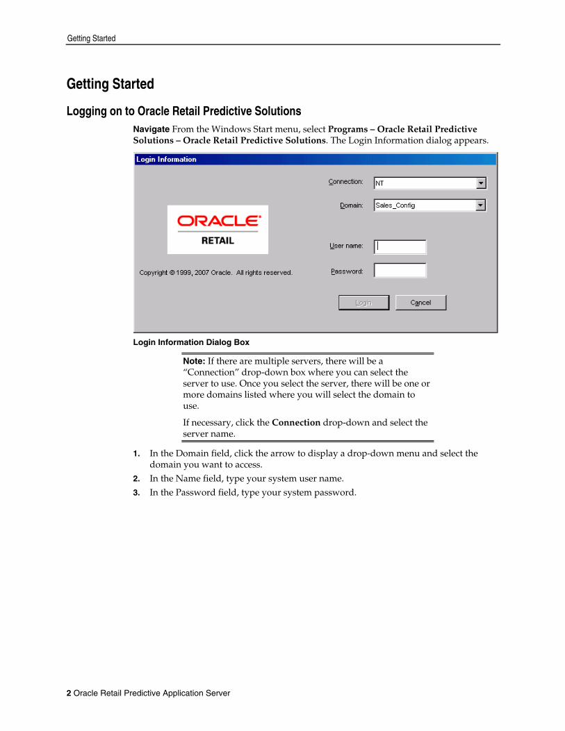
Logging on to Oracle Retail Predictive Solutions Navigate From the Windows Start menu, select Programs – Oracle Retail Predictive Solutions – Oracle Retail Predictive Solutions. The Login Information dialog appears.
Login Information Dialog Box
Note: If there are multiple servers, there will be a “Connection” drop-down box where you can select the server to use. Once you select the server, there will be one or more domains listed where you will select the domain to use.
If necessary, click the Connection drop-down and select the server name.
1. In the Domain field, click the arrow to display a drop-down menu and select the domain you want to access.
2. In the Name field, type your system user name. 3. In the Password field, type your system password.

Getting Started
Introduction 3
Note: One or more of the above fields may not be visible if your system has been configured to automatically populate these field values.
4. Click OK. The Oracle Predictive Solutions screen appears.
Oracle Predictive Solutions Screen

Getting Started
4 Oracle Retail Predictive Application Server
Changing Your Password Perform the procedure below to change your password.
Navigate From the File menu, select Change Password. The Change Password dialog box is displayed:
Change Password Dialog Box
1. In the Current Password field, type your old password. 2. In the New Password field, type the new password. 3. In the Verify New Password field, type the new password again. 4. Click OK.
Logging Off and Leaving the Login Information Screen Open Perform the following procedure to log off from the system and leave the Login Information screen open for use by another user or for logging on to another server.
Navigate From the File menu, select Logoff. If changes were made to an open workbook, the Close Workbook dialog appears.
Close Workbook Dialog Box
1. Select one of the radio buttons: Don't commit, Commit now, Commit ASAP, or Commit later. See Appendix A – Using RPAS Menus and Toolbars (subheading File Menu) – for an explanation of the terms Save and Commit.
2. Click Save, Don't Save, or Cancel.

Getting Started
Introduction 5
Logging Off and Exiting the System Follow this procedure to log off and exit the system completely.
Navigate From the File menu, select Exit. If changes were made to an open workbook, the Close Workbook dialog box appears.
Close Workbook Dialog Box
1. Select one of the radio buttons: Don't commit, Commit now, Commit ASAP, or Commit later. See Appendix A – Using RPAS Menus and Toolbars (subheading File Menu) – for an explanation of the terms Save and Commit.
2. Click Save, Don't Save, or Cancel.

Basic RPAS Concepts 7
2 Basic RPAS Concepts
Multidimensional Databases Multidimensional database systems provide a multidimensional view of data. For predictive, planning, and analytical applications; a multidimensional database provides significant benefits over a relational database. Applications that run on RPAS use multidimensional databases to store data records in the master database, and multidimensional worksheets are used to present this data. This topic compares multidimensional and relational databases, and it describes the fundamental aspects of multidimensional databases, such as dimensions and hierarchies.
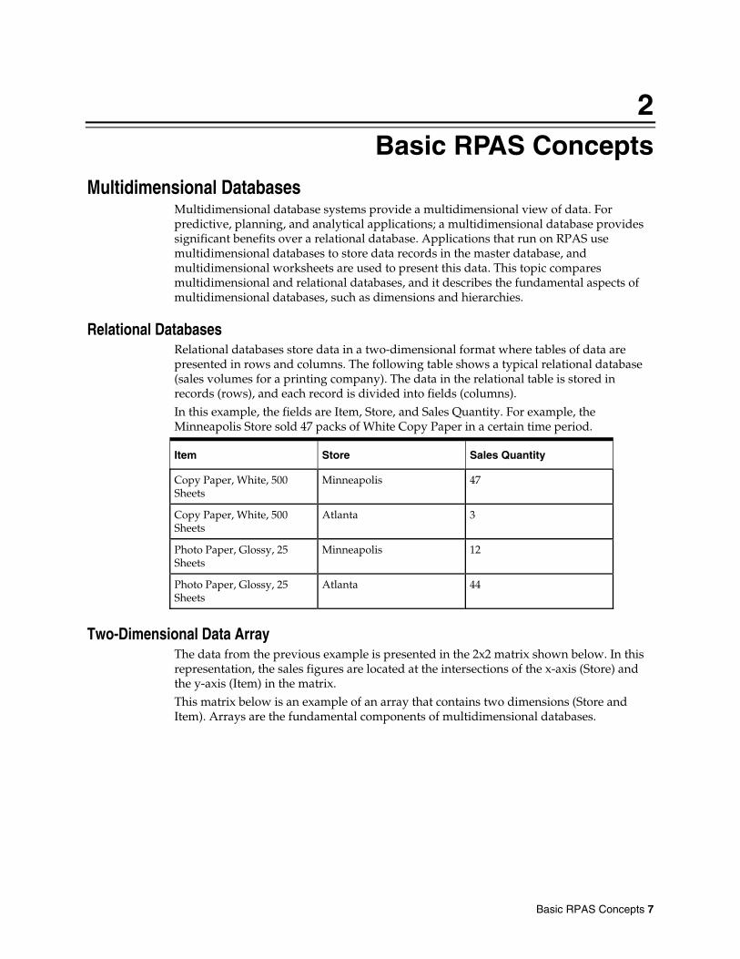
Relational Databases Relational databases store data in a two-dimensional format where tables of data are presented in rows and columns. The following table shows a typical relational database (sales volumes for a printing company). The data in the relational table is stored in records (rows), and each record is divided into fields (columns). In this example, the fields are Item, Store, and Sales Quantity. For example, the Minneapolis Store sold 47 packs of White Copy Paper in a certain time period.
Item Store Sales Quantity
Copy Paper, White, 500 Sheets
Minneapolis 47
Copy Paper, White, 500 Sheets
Atlanta 3
Photo Paper, Glossy, 25 Sheets
Minneapolis 12
Photo Paper, Glossy, 25 Sheets
Atlanta 44
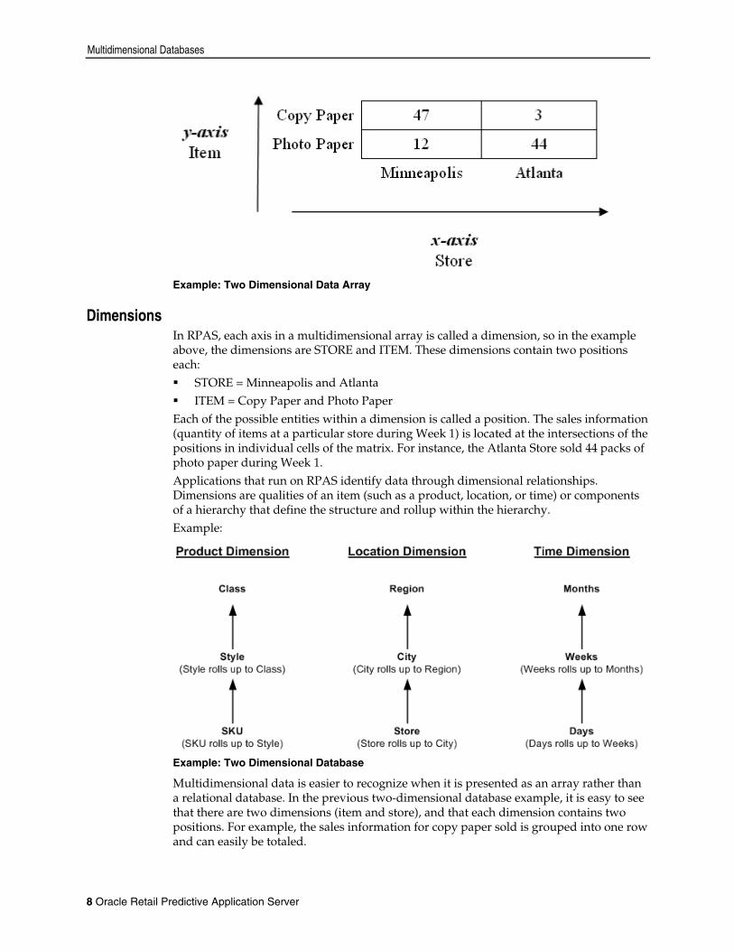
Two-Dimensional Data Array The data from the previous example is presented in the 2x2 matrix shown below. In this representation, the sales figures are located at the intersections of the x-axis (Store) and the y-axis (Item) in the matrix. This matrix below is an example of an array that contains two dimensions (Store and Item). Arrays are the fundamental components of multidimensional databases.
Multidimensional Databases
8 Oracle Retail Predictive Application Server
Example: Two Dimensional Data Array
Dimensions In RPAS, each axis in a multidimensional array is called a dimension, so in the example above, the dimensions are STORE and ITEM. These dimensions contain two positions each: STORE = Minneapolis and Atlanta ITEM = Copy Paper and Photo Paper
Each of the possible entities within a dimension is called a position. The sales information (quantity of items at a particular store during Week 1) is located at the intersections of the positions in individual cells of the matrix. For instance, the Atlanta Store sold 44 packs of photo paper during Week 1. Applications that run on RPAS identify data through dimensional relationships. Dimensions are qualities of an item (such as a product, location, or time) or components of a hierarchy that define the structure and rollup within the hierarchy. Example:
Example: Two Dimensional Database
Multidimensional data is easier to recognize when it is presented as an array rather than a relational database. In the previous two-dimensional database example, it is easy to see that there are two dimensions (item and store), and that each dimension contains two positions. For example, the sales information for copy paper sold is grouped into one row and can easily be totaled.

Multidimensional Databases
Basic RPAS Concepts 9
The array format displays immediate information about the number of dimensions in the data and the number of positions within each dimension. Therefore, arrays are far more organized than relational tables, and they ease data analysis and retrieval by eliminating the need to search individual records. By storing data in an array format, systems can quickly and efficiently import and export data in a nightly batch process, which allows the accumulating and spreading of data to take place very quickly.
Three-Dimensional Relational Table The relational database example can be extended by adding a third dimension to the data set. In the following example, the dimension “Customer Type” is added to the table. This dimension contains two possible positions (Trade Business and General Public Business). The addition of one dimension with two positions actually doubles the number of rows in the table. This method of presenting data is difficult to handle because the table’s length expands considerably with the addition of each new dimension. This is why RPAS uses a multidimensional structure, which is explained in the following section.
Item Store Customer Type Sales Quantity
Copy Paper, White, 500 Sheets
Minneapolis Trade 47
Copy Paper, White, 500 Sheets
Minneapolis General Public 23
Copy Paper, White, 500 Sheets
Atlanta Trade 3
Copy Paper, White, 500 Sheets
Atlanta General Public 17
Photo Paper, Glossy, 25 Sheets
Minneapolis Trade 12
Photo Paper, Glossy, 25 Sheets
Minneapolis General Public 43
Photo Paper, Glossy, 25 Sheets
Atlanta Trade 44
Photo Paper, Glossy, 25 Sheets
Atlanta General Public 41
How Multidimensional Databases Handle Additional Dimensions A multidimensional structure accepts the addition of new dimensions while providing the ease of data analysis. There is now a three-dimensional 2x2x2 array (see the illustration below) that contains 8 cells rather than a two-dimensional (4x8) array that contains 32 data cells. The data is still sorted and presented in the same manner. The following figure shows a three-dimensional data array.

Hierarchies
10 Oracle Retail Predictive Application Server
Example: Three-dimensional Array
Four-Dimensional Data Array The three-dimensional data array can be expanded to four dimensions by adding the dimension of time. Four dimensions are more difficult to understand, so imagine an array that is similar to the figure below for each of the twelve months of the year (twelve positions in the time dimension).
Example: Four-dimensional Array
Hierarchies Hierarchies are a top-to-bottom set up of parent-child relationships between levels that belong to the same entity (for example; time = years, months, weeks, and days). Organizations use these structures to describe relationships between the many dimensions. A hierarchy provides a means to define relationships between dimensions by aggregates (roll ups, and alternate roll ups). RPAS hierarchies reflect the hierarchies used in retailer’s operational systems, such as the Oracle Retail Merchandising System (RMS). If you use RPAS in conjunction with RMS, the hierarchies will usually default to the RMS hierarchical structure.

Hierarchies
Basic RPAS Concepts 11
The figure below (left) illustrates a sample RMS product hierarchy. The RMS hierarchy may also be augmented to include other rollups and attributes, such as product status or price point. In the diagram on the right, the Style dimension contains an alternate roll-up to the Supplier dimension. Each position in the Style dimension will have one parent position in the Subclass dimension and one in the Supplier dimension.
Example: RMS Product Hierarchy
Hierarchy Rules Generally, hierarchies are far more complex than those in the previous examples. An item at a particular level in a hierarchy can be aggregated along several hierarchical paths. However, for any given roll-up path, that item can only belong to one parent at any higher dimensional level. For example, if a given store location is aggregated to the state level, that location can only belong to one state position (for instance, Georgia or Florida, but not both). You can view data at any level of detail by drilling down or rolling up through levels in the hierarchy. Hierarchies define the path of data aggregation and spreading.
Workbooks, Worksheets, and Wizards
12 Oracle Retail Predictive Application Server
Workbooks, Worksheets, and Wizards
Workbooks The Oracle Retail Predictive Solutions integrate and manipulate your organization’s planning and forecasting data and presents it in a workbook format. A workbook is a local copy of the data of record in the domain that the end user can easily view and manipulate. Its multidimensional framework is used to perform specific business functions, such as generating sales forecasts and building merchandise financial plans. To present data, a workbook can contain any number of multidimensional spreadsheets, called worksheets, as well as graphical charts and related reports. These components work together to ease the viewing and analysis of business functions. Once the workbook framework and its specific attributes have been defined and built, the structure is saved as a workbook template; which allows new sets of data to be imported, manipulated, and presented as needed in a standardized format. This approach has the following advantages: It eliminates the need to redefine workbook parameters whenever you want to view
a new set of data. It ensures that the calculations are correct. It imposes a standard approach on all users to the business process.
Remember that data in a workbook can be viewed at lower levels of detail or higher levels of aggregation. Different views are obtained by changing the path and/or the level of data rollup. Data in a workbook can also be manipulated at any hierarchical level. If you modify data at an aggregate level, these changes are distributed down to the lower levels. The reverse is also true — if you modify data at a lower level in the hierarchy, the aggregates of the data reflect those changes.
Building Workbooks Workbooks can either be built in two ways: 1. Automatically during nightly batch runs. 2. Manually by using a wizard. The Workbook Auto Build feature allows you to set up workbook builds, which take place on a regular basis during nightly batch runs. Workbooks to be built in this way are added to the auto build queue. This way, you are spared the processing time that is required to regularly enter the same selections, and you are spared the wait time associated with workbook builds.
Worksheets Worksheets are multidimensional spreadsheets that are used to display information from the workbook. Workbooks can include one worksheet or multiple worksheets, which can present data in the form of numbers in a grid. These numeric data values can easily be converted to a graphical chart. Data can be viewed at a very high level of detail, or data values can be quickly aggregated and viewed at summary levels. You can display the information in a worksheet in a variety of formats; generally by rotating, changing the data rollup, showing and hiding measures, and drilling up or down. The Oracle Retail Predictive Solutions also allow you to easily change the presentation style of data in a worksheet.
Menus, Quick Menus, and Toolbars
Basic RPAS Concepts 13
Wizards A wizard is a feature that steps you through the process of building a new workbook from a workbook template. A wizard displays successive dialogs that require you to answer a sequence of questions or enter selections regarding the content of your workbook. Your responses to these questions are used to automatically format and populate the workbook that you want to build. The specific information required by a wizard depends on the type of workbook being built. For example, the wizard might ask you to select the hierarchy level at which a source forecast should be run, or it may ask you to select the products and/or locations that should be included in a particular workbook. A variety of workbook templates may exist for building different types of workbooks for each application. In addition, there are workbook templates for performing system administration and data maintenance on the Administration and Analysis tabs, respectively.
Menus, Quick Menus, and Toolbars
Menus Standard pull-down menus are available for performing most commands. Click on the appropriate menu title in the application’s menu bar to display the menu. Some applications may have added further menu options to those provided as standard by the platform.
Quick Menus Quick menus (right-click menus) are available to access certain commands. To access a quick menu, right-click over an appropriate screen area. These quick menus are context-sensitive, which means their availability, appearance, and options depend on the screen area where you right-clicked. Quick menus are essential tools for functions, such as: Changing the level and/or path of hierarchy rollup Hiding positions within a dimension Switching the view of your worksheet between outline view and block view Sorting or resorting data in a dimension Formatting grid and chart data
Toolbars The RPAS toolbar contains iconic buttons (having the character of an icon) that give you direct access to many common commands and actions. To see the function of a particular toolbar button, move your cursor to a position above it. A caption describing the button’s function will appear in the status bar at the bottom of the screen.


Using Workbooks, Worksheets, and Wizards 15
3 Using Workbooks, Worksheets, and Wizards
Using Workbooks and Worksheets
Overview Once you log on to RPAS, the Oracle Predictive Solutions window appears.
Oracle Predictive Solutions Window
Menu Bar
Overview The menu bar is displayed under the workbook title bar. To access a particular command, left-click once on the menu label. A pull-down menu of options that are specific to that section is displayed. The choices of the menu are context-sensitive, meaning that the choices and their availability change depending on your current selection or mode of work. When an item is grayed-out, it is not available in your current selection or mode of work.
File Menu When the File menu is selected, the File menu options appear.

Using Workbooks and Worksheets
16 Oracle Retail Predictive Application Server
File Menu Options
Note: Save, Commit, and Print options are added to the menu when a workbook is open. The New File menu is discussed in detail in Appendix A – Using RPAS Menus and Toolbars.
File - New The New menu option allows you to create a new workbook. When you select File – New, the New dialog box appears.
New Dialog Box
Note: File – New gives the same results as the selecting the New button from the toolbar.
The New dialog box, shown below, is a generic example. The tabs within this box are specific to the client configuration. There can be a number of tabs.
See “The New Dialog Box” for a description of the tabs.

Using Workbooks, Worksheets, and Wizards
Using Workbooks, Worksheets, and Wizards 17
File - Open The Open menu option allows you to open an existing workbook. When you select File – Open, the Open dialog appears.
Open Dialog Box
This dialog box displays all of the workbooks that you are allowed to open. This includes all workbooks that you have created and saved, and not yet deleted. It also includes any workbooks that other users have saved with World Access. To open a workbook, highlight the selection you want to view, and click OK. When you view the list of available workbooks, click on any column header to sort the workbooks by that attribute. For example, click the Owner column header to sort the workbooks alphabetically by owner. Select List all workbooks option to display all workbooks in the system. This includes those that you do not have write access to. Listing those additional workbooks does not give you write access to them.
Note: File – Open gives the same results as the Open button.
File - Delete The Delete menu option allows you to delete existing workbooks. When you select File – Delete, the Delete dialog appears.

Using Workbooks and Worksheets
18 Oracle Retail Predictive Application Server
Delete Dialog Box
Note: File – Delete gives the same results as the Delete button.
This dialog lists all of the workbooks that you are allowed to delete. This includes all workbooks that you have created and saved, and not yet deleted. It also includes any workbooks that other users have saved with World Access. To delete a workbook, select the workbook you want to delete, and click OK.
Delete Workbooks
Navigate From the File menu, select Delete. 1. Select the workbook or workbooks to delete.
Note: Deleted workbooks are permanently removed from the system.
2. Click OK. 3. Click OK again to confirm the deletion.
File - Commit Status The Commit Status menu option allows you to see the status of recent commit processes that used the Commit ASAP functionality. See "File – Commit ASAP" in Appendix A –

Using Workbooks, Worksheets, and Wizards
Using Workbooks, Worksheets, and Wizards 19
Using RPAS Menus and Toolbars. When you select File – Commit Status, the Commit Status dialog box appears.
Commit Status Dialog Box
This dialog is available whether or not you have a workbook open. The dialog box shows the following information about each commit request: Workbook Name
– An unsaved workbook committed with Commit ASAP is assigned a Workbook Name of "untitled."
Template Name Submission Time Owner Submitter Status Completion Time
At the bottom of the Commit Status window, you can filter the commit requests to view based on their status. To update the workbooks based on your selected filter criteria, click Refresh. Workbooks may display the following status: Pending – The commit is queued up to take place at some point in the future Committing – The workbook is currently being committed Successful – The commit succeeded Failed – The commit failed
Columns in the Commit Status dialog box can be selected and the displayed data will be immediately sorted in ascending or descending order. Data is refreshed and re-displayed when you click Refresh . This is useful when: You have changed the filters. You need to watch for a commit that is pending. You need to see when committing completes.
RPAS retains and displays the details of the last 1000 successful and unsuccessful commit ASAP process for the domain. Old details will automatically be removed from this status report in a time period that depends on the level of commit ASAP activity for the domain as a whole.

Using Workbooks and Worksheets
20 Oracle Retail Predictive Application Server
Note: Commit Now and Commit Later actions will not display in the Commit Status dialog box. There can only be one pending commit ASAP in the queue for a given workbook/user/template name combination. If a subsequent commit ASAP is issued before the first has executed, the first commit ASAP is removed from the queue and will never get processed. The new commit ASAP is placed at the end of the queue.
File - Change Password The Change Password menu option allows you to change your password. See "Changing Your Password" in the Getting Started section.
Note: RPAS can be installed as a web-based application (see the RPAS Administration Guide for more information). The Change Password menu option is disabled for web-based users.
File - Logoff The Logoff menu option allows you to logoff from the system. If you have a workbook open, the Close Workbook dialog appears when you select File – Logoff.
Close Workbook Dialog Box
If you do not have a workbook open, a message box appears when you select File – Logoff.
Logoff Verification Dialog Box
This is one of two methods that you can use to log off of the system. When you select this option, you will be logged off, but the Login Information dialog box is still displayed. This leaves the system ready for another user to access.

Using Workbooks, Worksheets, and Wizards
Using Workbooks, Worksheets, and Wizards 21
If you have an unsaved workbook open at the time you select Logoff, the Close Workbook dialog box appears. Select the required commit activity, and select Save or Don't Save as required, or select Cancel to cancel the Logoff request.
File - Exit The Exit menu option allows you to logoff and exit from the system. If you have a workbook open, the Close Workbook dialog appears when you select File – Exit.
Close Workbook Dialog Box
If you do not have a workbook open, a message box appears when you select File – Exit.
Logoff Verification Dialog Box
File – Exit is the second of two methods that you can use to log off the system. The Exit option logs you off of the application and exits the system completely. If you have an unsaved workbook open at the time you select Exit the Close Workbook dialog box appears. Select the required commit activity, and click on Save or Don't Save as required, or select the Cancel button to cancel the Exit request.
View Menu When you click View, the View menu options appear:
View Menu Options

Using Workbooks and Worksheets
22 Oracle Retail Predictive Application Server
Note: Grid/Chart toggle, Zoom, Alert, and Flow control options are added to the menu when a workbook is open. This is discussed in detail in Appendix A ─ Using RPAS Menus and Toolbars.
The following topics provide brief descriptions of the View menu options.
View – Alert Manager The Alert Manager menu option displays the Alert Manager window, or it hides it if it is already displayed. When you select View – Alert Manager, the Alert Manager window appears (if it is not already visible).
Alert Manager Window
Note: See “Alert Manager” under the heading “The New Dialog Box”.
View – Full Screen The Full Screen menu option hides the status bar, the tool bar, and the application title. The window is maximized to fill the entire screen. Click this option again to return the window to its original size.
View – Status Bar The Status Bar menu option displays or hides the status bar at the bottom of the application window.
View – Toolbar The Toolbar menu option displays or hides the toolbar at the top of the application window.
Format Menu When you click Format, the Format menu options appear.

Using Workbooks, Worksheets, and Wizards
Using Workbooks, Worksheets, and Wizards 23
Format Menu Options when No Workbooks Open
Note: Axis, Measure, Grid, Exceptions, Types, Workbook and Format Save/Delete options are added to the menu when a workbook is open. The new Format menu is discussed in detail in Appendix A ─ Using RPAS Menus and Toolbars.
Format – Application Selecting Format – Application, displays the Format Options dialog box.
Format Options Dialog Box – Application Tab Selections made on the Application tab affect all worksheets in the current workbook. The Application option on the Format menu is only available in Grid view (not Chart view).
To change the view from Chart to Grid, click the Toggle button , or select View – Grid. The Format Options dialog box displays the following options and functionality:
Color Options
Grid background color
This option sets the color for the area within a worksheet window that lies beneath the grid display, column/row/slice axes, hierarchy tiles, and scroll bars. Deferred calculation color
Using Workbooks and Worksheets
24 Oracle Retail Predictive Application Server
This option sets the background color for cells in which a deferred calculation is pending. The color chosen from this palette is only displayed if the “Show Deferred Calculation Color” check box (described below) is selected. The “Deferred Calculation Color” overrides the “Read/Write Color” selection for a cell. Read-only color This option sets the color for read only worksheet cells. Read/write color This option sets the color for read/write worksheet cells.
Note: The Read/Write Color option will be overridden if a workbook is open and the Shade Colors By Dimension option on the Format – Axis tab is selected. Dimension shading (if toggled on) overrides any read/write color selection, but it does not override the read only color selection. If it appears that your read/write color selection is not recognized by the system, try toggling off the Shade Colors By Dimension option on the Format – Axis tab.
Application Options
Show Elapsed Locks When this box is unchecked, elapse positions will only be the ‘Read Only’ color. When the box is checked, elapse positions will be the ‘Read Only’ color with the elapsed lock
. Show Button Text This option toggles the display of toolbar button titles. If this check box is selected, the toolbar buttons appear large and include the button name/function. If this check box is cleared, the toolbar buttons appear small and do not contain text. Show Deferred Calculation Color This option toggles the display of a distinctive background color for cells in which a deferred calculation is pending. The color for such cells is specified by using the Deferred Calculation Color option described above. When the Show Deferred Calculation Color check box is selected, the selected color is displayed whenever applicable. Show Tab Control For workbook templates that support process tab control, you have the option of disabling the tab control display. Check this check box to turn on the tab control bar. Remove the check box to turn off the display. When the tab control bar is not displayed, the Previous and Next buttons are still present on the application toolbar, which enables you to advance through the workbook process flow. Prompt for Deferred Calculations There are some actions (such as opening another minimized worksheet) that require that there are no cell edits that have not yet been calculated. In such circumstances, this option allows you to enable or disable the display of a warning dialog. When the Prompt for Deferred Calculations box is selected, the Calculate Workbook dialog box appears which allows you to cancel the action if necessary.

Using Workbooks, Worksheets, and Wizards
Using Workbooks, Worksheets, and Wizards 25
Calculate Working Dialog Box
For the above warning to be displayed, you must first edit a cell in a worksheet (for instance, changing the administrative rights from Full Access to Denied). Then certain actions (such as closing the worksheet) will cause the warning to be displayed.
Note: If you select the Don't show this message again option, the system automatically defaults to Yes.
Click Yes to retain and calculate the changes. Click No to discard the changes. Click Cancel to cancel the operation.
Collapse Positions by Default When dimensions are expanded (showing parent-child relationships), and you place a check in the “Collapse Positions by Default” checkbox, these positions will collapse causing the child positions to get rolled up into their parent positions. In the following illustration, “Jackets” rolls up into Men’s Sportswear, “Casual” rolls up into Footwear Men’s, and so on.
When the box is checked.
When the box is not checked.
Using Workbooks and Worksheets
26 Oracle Retail Predictive Application Server
Auto position query evaluation RPAS supports the use of Position Queries to drive the positions that are visible on a window. Those position queries are updated when certain events occur, such as changing the ‘driver’ position in the Z-axis while the view is opened. By enabling “Auto position query evaluation” the visible positions are updated when the associated Boolean measure is changed as the result of a calculation. For performance reasons, this option is disabled by default. A new position query button is displayed when there are position queries on the Z-axis of the worksheet. If this button is disabled, the position queries are up to date. If this button is enabled, which can only happen if the auto evaluation option is off, the position queries need to be updated by clicking the button.
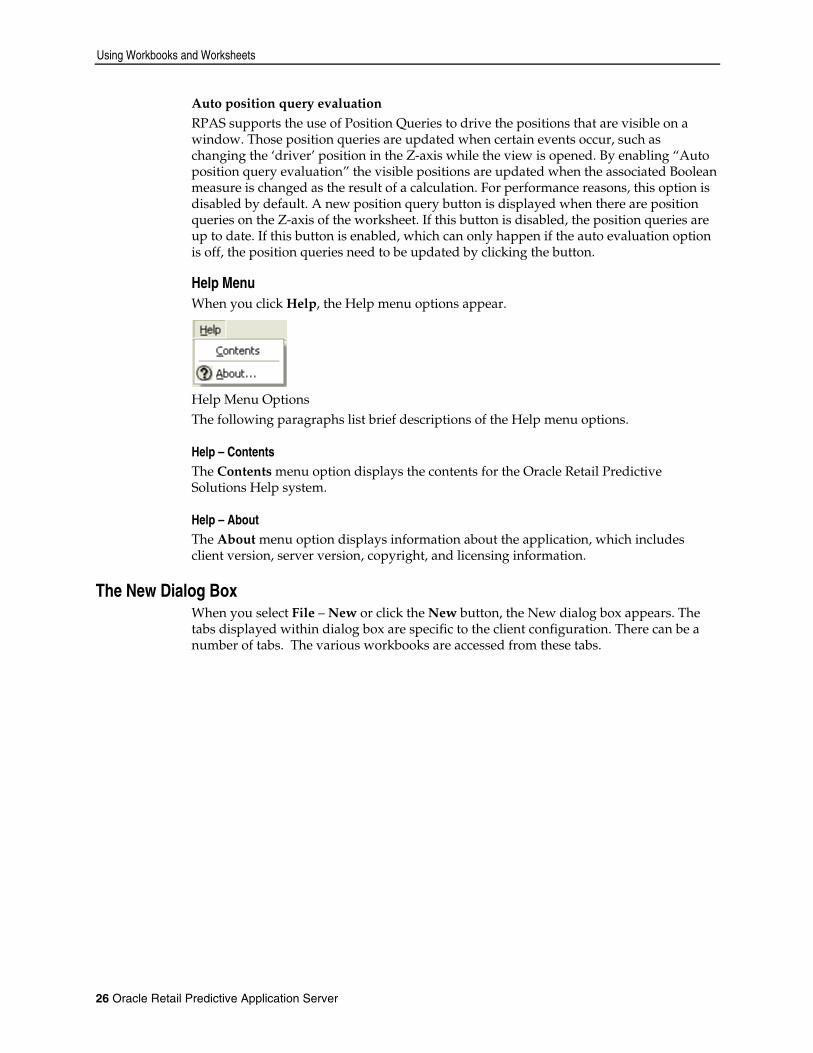
Help Menu When you click Help, the Help menu options appear.
Help Menu Options The following paragraphs list brief descriptions of the Help menu options.
Help – Contents The Contents menu option displays the contents for the Oracle Retail Predictive Solutions Help system.
Help – About The About menu option displays information about the application, which includes client version, server version, copyright, and licensing information.
The New Dialog Box When you select File – New or click the New button, the New dialog box appears. The tabs displayed within dialog box are specific to the client configuration. There can be a number of tabs. The various workbooks are accessed from these tabs.
Using Workbooks, Worksheets, and Wizards
Using Workbooks, Worksheets, and Wizards 27
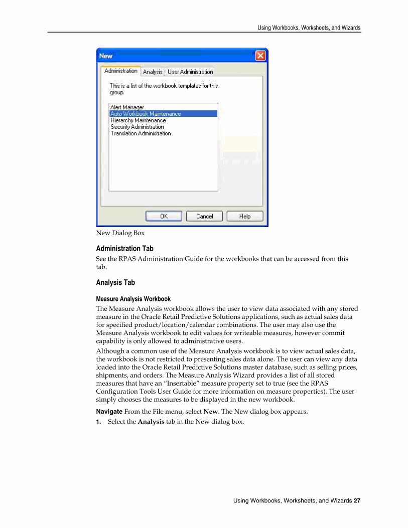
New Dialog Box
Administration Tab See the RPAS Administration Guide for the workbooks that can be accessed from this tab.
Analysis Tab
Measure Analysis Workbook The Measure Analysis workbook allows the user to view data associated with any stored measure in the Oracle Retail Predictive Solutions applications, such as actual sales data for specified product/location/calendar combinations. The user may also use the Measure Analysis workbook to edit values for writeable measures, however commit capability is only allowed to administrative users. Although a common use of the Measure Analysis workbook is to view actual sales data, the workbook is not restricted to presenting sales data alone. The user can view any data loaded into the Oracle Retail Predictive Solutions master database, such as selling prices, shipments, and orders. The Measure Analysis Wizard provides a list of all stored measures that have an “Insertable” measure property set to true (see the RPAS Configuration Tools User Guide for more information on measure properties). The user simply chooses the measures to be displayed in the new workbook.
Navigate From the File menu, select New. The New dialog box appears. 1. Select the Analysis tab in the New dialog box.

Using Workbooks and Worksheets
28 Oracle Retail Predictive Application Server
New Dialog Box – Analysis Tab
2. Select Measure Analysis, and click OK. The Measure Analysis Wizard opens.
Measure Analysis Wizard - Select Measures Screen
Using Workbooks, Worksheets, and Wizards
Using Workbooks, Worksheets, and Wizards 29
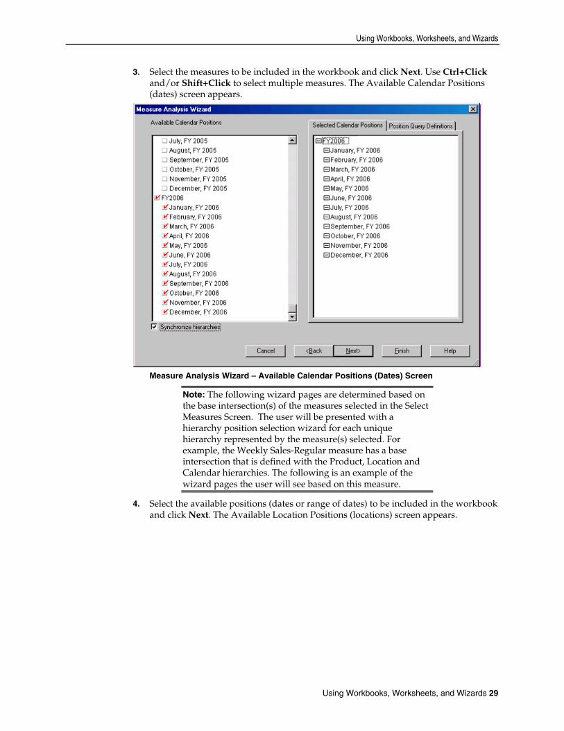
3. Select the measures to be included in the workbook and click Next. Use Ctrl+Click and/or Shift+Click to select multiple measures. The Available Calendar Positions (dates) screen appears.
Measure Analysis Wizard – Available Calendar Positions (Dates) Screen
Note: The following wizard pages are determined based on the base intersection(s) of the measures selected in the Select Measures Screen. The user will be presented with a hierarchy position selection wizard for each unique hierarchy represented by the measure(s) selected. For example, the Weekly Sales-Regular measure has a base intersection that is defined with the Product, Location and Calendar hierarchies. The following is an example of the wizard pages the user will see based on this measure.
4. Select the available positions (dates or range of dates) to be included in the workbook and click Next. The Available Location Positions (locations) screen appears.
Using Workbooks and Worksheets
30 Oracle Retail Predictive Application Server
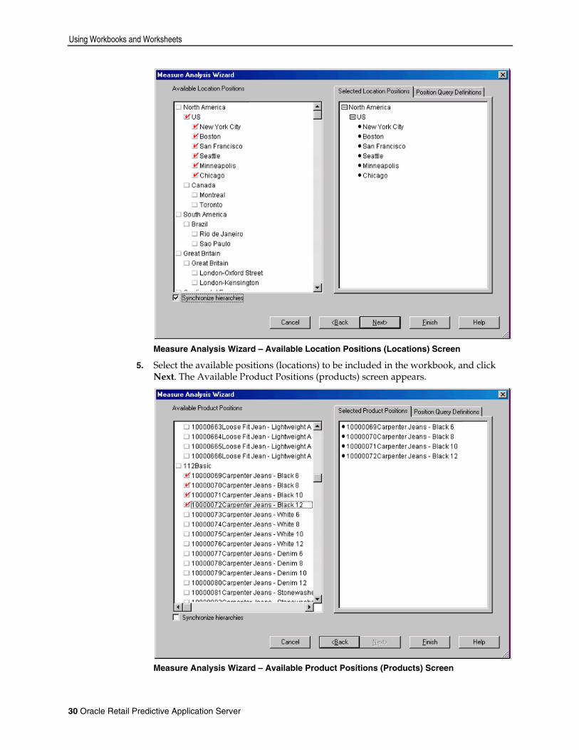
Measure Analysis Wizard – Available Location Positions (Locations) Screen
5. Select the available positions (locations) to be included in the workbook, and click Next. The Available Product Positions (products) screen appears.
Measure Analysis Wizard – Available Product Positions (Products) Screen

Using Workbooks, Worksheets, and Wizards
Using Workbooks, Worksheets, and Wizards 31
6. Select the available positions (products) to be included in the workbook, and click Finish. The Measure Analysis Workbook is built.
Example of Measure Analysis Worksheet
7. Edit the writable cells for the measure(s) that you selected as necessary. Commit capability will be enable for administrative users.
8. Select Close from the File menu to close the workbook. The Calculate Workbook dialog box appears.
Calculate Workbook Dialog Box
9. Click Yes. The Close Workbook dialog box appears.

Using Workbooks and Worksheets
32 Oracle Retail Predictive Application Server
Close Workbook Dialog Box
10. Select Commit Now, and click Save if the workbook is to be saved. The Save As dialog box appears.
Save As Dialog Box
11. Enter the name your workbook in the Workbooks field, and click OK. A message box appears to inform you that the data updates were successfully committed.
Using Workbooks, Worksheets, and Wizards
Using Workbooks, Worksheets, and Wizards 33
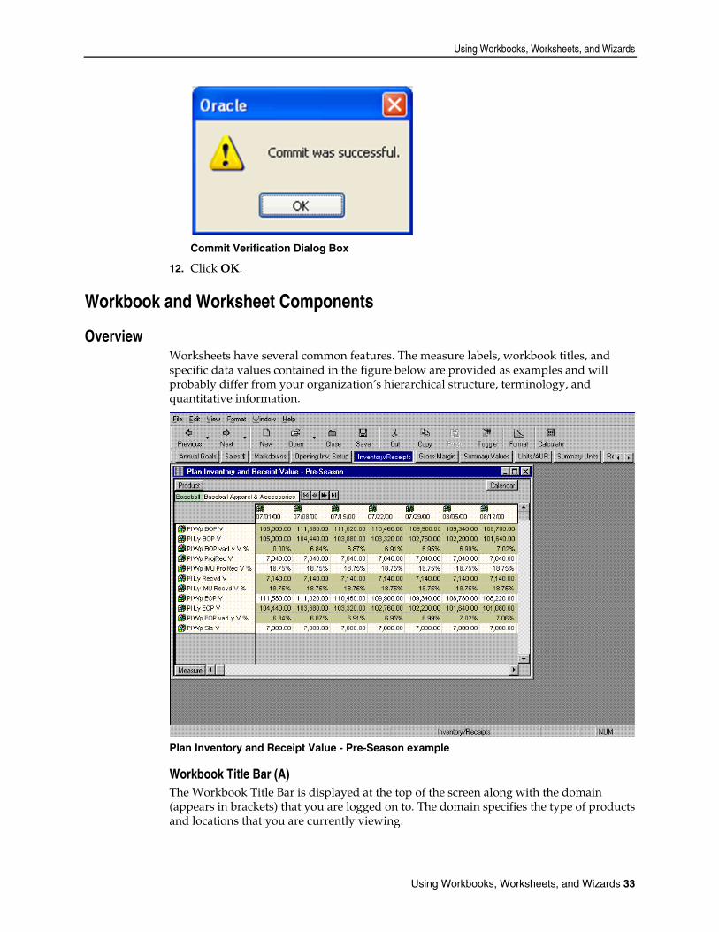
Commit Verification Dialog Box
12. Click OK.
Workbook and Worksheet Components
Overview Worksheets have several common features. The measure labels, workbook titles, and specific data values contained in the figure below are provided as examples and will probably differ from your organization’s hierarchical structure, terminology, and quantitative information.
Plan Inventory and Receipt Value - Pre-Season example
Workbook Title Bar (A) The Workbook Title Bar is displayed at the top of the screen along with the domain (appears in brackets) that you are logged on to. The domain specifies the type of products and locations that you are currently viewing.

Workbook and Worksheet Components
34 Oracle Retail Predictive Application Server
Menu Bar (B) The menu bar is displayed under the worksheet title bar. To access a particular command, left-click once on the menu label. A pull-down menu of options that are specific to that section is displayed. The choices of the menu are context-sensitive, meaning that the choices and their availability change depending on your current selection or mode of work. When an item is grayed-out, it is not available in your current selection or mode of work.
Toolbar (C) The RPAS toolbar contains iconic buttons (having the character of an icon) that give you direct access to many common commands and actions. To see the function of a particular toolbar button, move your cursor to a position above it. A caption describing the button’s function will appear in the status bar at the bottom of the screen.
Worksheet Title Bar (D) The title of the current worksheet is displayed here.
Flow Control Worksheet Tabs (E) There is a row of flow control worksheet tabs located near the top of the application window and beneath the toolbar. Each tab represents a distinct step in the business process that has been configured for your solution, and the tabs will usually be ordered in a logical progression of necessary steps. Each tab (or step) is associated with one or more separate worksheets. Click on a flow control tab to access the worksheet(s) that Toolbar are relevant to that step in the planning process. When building a new workbook, the worksheet associated with each flow control tab may initially be minimized. When a worksheet is minimized, an icon representing that worksheet is displayed near the bottom of the screen. Double-click the icon to expand the worksheet to full view.
Display Worksheets from Different Flow Control Process Steps When you click a specific tab in the flow control, only those worksheets associated with that process step are automatically available for view. If you want to simultaneously view two or more worksheets that are associated with different flow control tabs, you must display the relevant worksheet for one business step, and then use the Unhide option on the Window menu to display any of the workbook’s other worksheets (even those related to other flow control steps). The system treats all worksheets that are not associated with the currently selected flow control step as if they are hidden. Therefore, any worksheet is available for view in a non-standard flow control step when you select that worksheet from the list provided on the Unhide dialog.
Status Bar The status bar at the bottom of the worksheet window displays logon/logoff notifications, warnings, and other system messages. If a pull-down menu is currently expanded and the cursor is placed over any of that menu’s available command options, the status bar will display a brief description of that menu option’s function.
Hierarchy Tiles and Display Area Hierarchies are the structures used by an organization to describe the relationships that exist between the many dimensions. Typically, any dimension will belong to one of the following four hierarchies displayed below.

Using Workbooks, Worksheets, and Wizards
Using Workbooks, Worksheets, and Wizards 35
Hierarchy Tiles
There may be others, but these are the most common. These hierarchies are represented on the worksheet by hierarchy tiles that represent each hierarchy. Hierarchy tile positions designate the worksheet axis where a particular hierarchy’s information is displayed. To change the orientation of data in a worksheet, drag and drop the hierarchy tiles to reposition them. The hierarchy tiles that you will see in Oracle Retail Predictive Solutions include: Hierarchy tiles can reside in the Row Display Area, the Column Display Area, or the Slice Display Area. The location of a hierarchy tile determines how the tile’s associated data is displayed. Data that is presented on the screen can be viewed in any format when you reposition the hierarchy tiles on the worksheet screen. A row display area, which is located at the bottom left corner of the worksheet, is one of three portions of the worksheet that contain the hierarchy tiles. Positions in hierarchies with tiles in this location become the headers for rows of data, with all the data in a row being for a single position. The headings for these rows appear on the left side of the worksheet along the row axis. The column display area is located at the top right corner of the worksheet. Positions in hierarchies with tiles in this location become the headers for columns of data, with all the data in a column being for a single position. The headings for these columns appear across the top of the worksheet along the column axis. The slice display area is located at the top left corner of a worksheet. Moving a hierarchy tile to this location controls which hierarchies are displayed in the slice axis. Where one or more hierarchy tiles are in the slice display area, all the worksheet data is for just a single position in those hierarchies, with the current position (the ‘context’) shown in the VCR control. The worksheet can be considered to be a single ‘page’ of data, with one page being available for all the combinations of positions in the hierarchies in the slice display area. The row axis of the worksheet displays the contents and dimensions of the hierarchy tiles that are currently in the row display area. Data for these dimensions are presented in rows, and the labels for each row position appear down the left side of the worksheet. The column axis of the worksheet displays the contents and dimensions of the hierarchy tiles that are currently in the column display area. Data for these dimensions are presented in columns, and the labels for each column position appear across the top of the worksheet.
Slice Axis and Scroll Bar The slice axis, which runs perpendicular to the plane of the computer screen, is necessary for the system to present multidimensional data on your two-dimensional monitor. A slice is like a page in a book. A separate page (or slice) exists for each element of the dimension represented by the hierarchy tile residing in the slice display area. The slice scroll bar works as a page-turner and is available when there is a hierarchy tile positioned in the slice display area. Click the right double triangles to page forward through data, and click the left double arrows to page back. The left line-arrow button moves you to the first page of data, and the right arrow-line button moves you to the last page of data.

Workbook and Worksheet Procedures
36 Oracle Retail Predictive Application Server
Vertical Scroll Bar The standard vertical scroll bar is used to navigate within the grid portion of the worksheet window. This scroll bar allows you to scroll up and down through the displayed data. The thumbtack (sliding control on the scrollbar) shows the viewing position on the screen relative to the full body of data. Perform the following functions on the vertical scroll bar: Click the thumbtack to press it. A pop-up caption displays the number of items along
that axis and the item number that you are currently viewing. Click the thumbtack and hold the mouse button down. Drag the thumbtack rapidly
to any location on the scroll bar. Release the mouse button to release the thumbtack. Click anywhere on the vertical scroll bar above the thumbtack to move up one page
of data at a time. Click anywhere on the vertical scroll bar below the thumbtack to move down one
page of data at a time.
Horizontal Scroll Bar The standard horizontal scroll bar is used to navigate within the grid portion of the worksheet window. This scroll bar allows you to scroll left and right through the displayed data. The thumbtack (sliding control on the scrollbar) shows the viewing position on the screen relative to the full body of data. Perform the following functions on the horizontal scroll bar: Click the thumbtack to press it. A pop-up caption displays the number of items along
that axis and the number that you are currently viewing. Click the thumbtack and hold the mouse button down. Rapidly drag the thumbtack
to any location on the scroll bar. Release the mouse button to release the thumbtack. Click anywhere on the horizontal scroll bar to the left of the thumbtack to move one
page of data to the left. Click anywhere on the horizontal scroll bar to the right of the thumbtack to move one
page of data to the right.
Workbook and Worksheet Procedures
Basic Workbook Procedures
Creating a New Workbook
Navigate From the File menu, select New. 1. Click the tab containing the workbook template group for the template you wish to
select. 2. Click on the workbook template for the workbook type you wish to build. 3. Click OK. 4. Follow the wizard instructions to create the workbook.
Using Workbooks, Worksheets, and Wizards
Using Workbooks, Worksheets, and Wizards 37
Opening a Workbook
Note: You are only allowed to open the following workbooks:
Those workbooks that you have created and saved. Those workbooks created by other users and saved with World access or Group
access for your group.
Navigate From the File menu, select Open. Select the workbook to open, and click OK.
Closing a Workbook
Navigate From the File menu, select Close. If changes were made to the workbook, select a button to save, commit, or ignore (discard) the changes.
Saving a Workbook
Navigate From the File menu, select Save. 1. If the Save As dialog box displays, type a name for the new workbook in the
Workbook Name field and select an access level for the workbook (User, Group, or World).
2. Click OK.
Note: Saving a workbook does not commit your changes to the master database.
Save a Workbook under a New Name
Navigate From the File menu, select Save As. 1. Type a new name for the workbook under Workbook Name. 2. Select an access level for the workbook (User, Group, or World), and click OK.
Revert to the Last Saved Version of a Workbook This procedure returns you to the most recently saved version of the workbook, discarding all changes made since the last save.
Navigate From the Edit menu, select Revert. Click OK.
Note: The Revert option is only enabled if the current workbook was already saved under a specified name, and if changes were made to the data since the last save.
Deleting a Workbook
Navigate From the File menu, select Delete. 1. Select the workbook or workbooks to delete.
Note: Deleted workbooks are permanently removed from the system.
2. Click OK. 3. Click OK again to confirm the deletion.
Workbook and Worksheet Procedures
38 Oracle Retail Predictive Application Server
Save and Delete Workbook Formats
Save a Workbook Format Use this procedure to save any formatting changes you have made to the workbook with the workbook template. Any new workbook that is created using the workbook template will default to this saved format. Saved information includes: Hierarchy and Measure Tile locations Visible dimensions (aggregate roll-ups) Measure order and format Window position and label Slice selection Block view vs. Outline view
Formats are saved for the specified workbook template only, and only affect newly built workbooks that were created from that same template. Saved formats do not affect any previously created and saved workbooks. If your access level is User, you can save user-level formats for your own use. If you have been granted Admin status, you can save default formats for all users. If a particular workbook template has both a user-level style and a template-level style saved for it, the format saved at user level overrides the format saved at the template level. You can also save formats at the group level. These changes apply to all users within that group.
Navigate From the Format menu, select Save Format. Select User level, Template level, or Group level depending on the level that you want to save the format. Select User if you want to save the format for your own use. Select Template if you have been granted Admin status, and you want to save the
format for global use. Select Group, and select from the list of available user groups if you want to save the
format for a user group.
Delete a Workbook Format Use this procedure to clear any formatting changes that you have previously saved. Format deletions only affect the workbook template that is associated with that format. For example, if you select Delete Format while viewing a Forecast Maintenance workbook, the deletion will only affect new Forecast Maintenance workbooks. If you have been granted Admin status, you can delete formats at both User level and Template level. If your access level is User, you can only delete formats for yourself. Deleting a format at Template level means that all new workbooks opened by any user using that same workbook template will no longer default to the deleted format. You can also delete formats for a user group. These changes apply to all users within that group.
Navigate From the Format menu, select Delete Format. Select User level, Template level, or Group level depending on the level that you want to delete the format. Select User if you want to delete a saved user format. Select Template if you want to delete a global format. This affects all other users who
build future workbooks using this template.
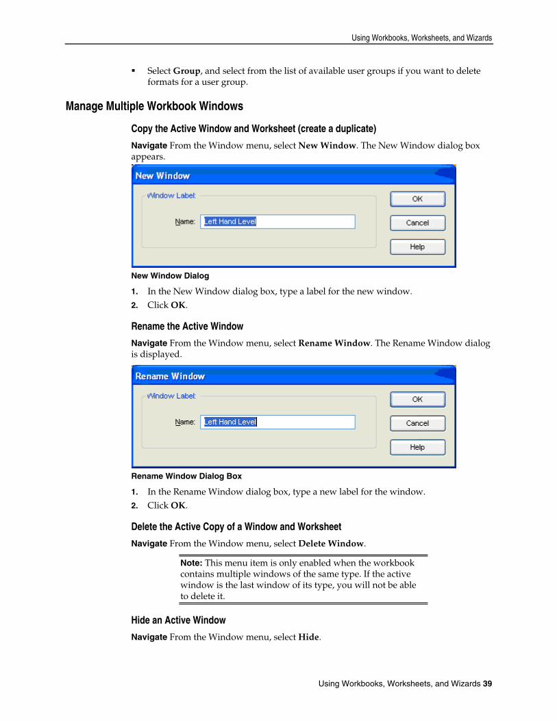
Using Workbooks, Worksheets, and Wizards
Using Workbooks, Worksheets, and Wizards 39
Select Group, and select from the list of available user groups if you want to delete formats for a user group.
Manage Multiple Workbook Windows
Copy the Active Window and Worksheet (create a duplicate)
Navigate From the Window menu, select New Window. The New Window dialog box appears.
New Window Dialog
1. In the New Window dialog box, type a label for the new window. 2. Click OK.
Rename the Active Window
Navigate From the Window menu, select Rename Window. The Rename Window dialog is displayed.
Rename Window Dialog Box
1. In the Rename Window dialog box, type a new label for the window. 2. Click OK.
Delete the Active Copy of a Window and Worksheet
Navigate From the Window menu, select Delete Window.
Note: This menu item is only enabled when the workbook contains multiple windows of the same type. If the active window is the last window of its type, you will not be able to delete it.
Hide an Active Window
Navigate From the Window menu, select Hide.
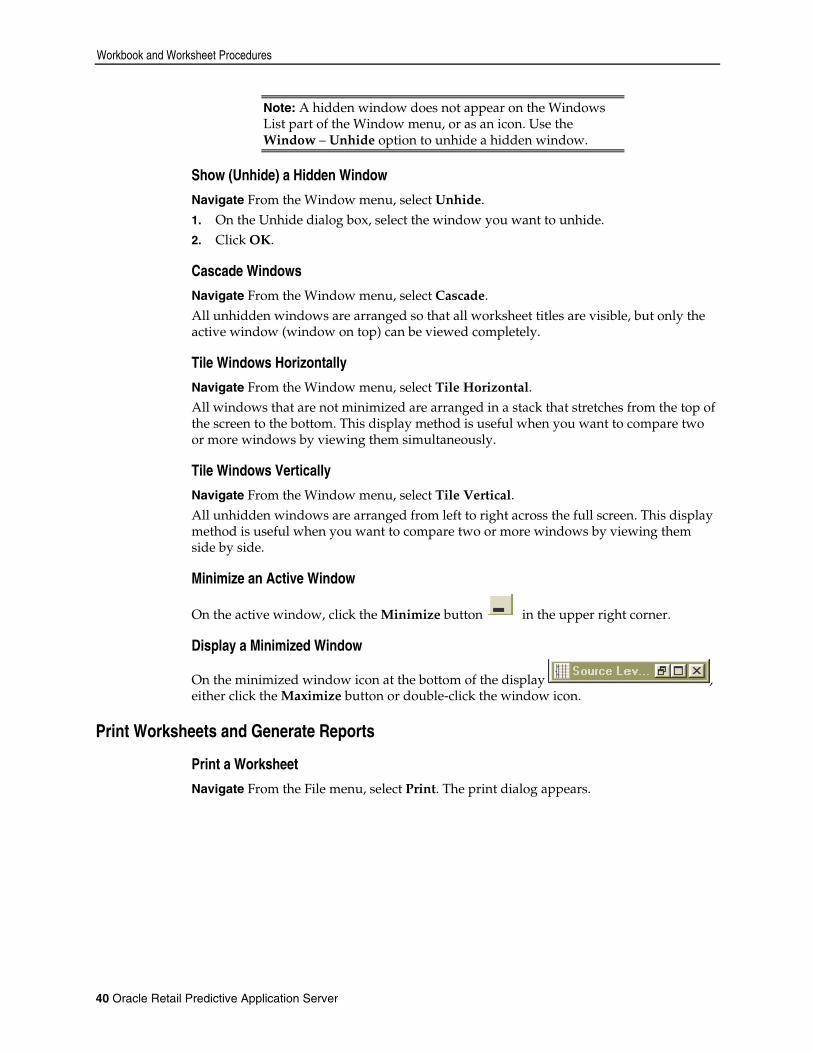
Workbook and Worksheet Procedures
40 Oracle Retail Predictive Application Server
Note: A hidden window does not appear on the Windows List part of the Window menu, or as an icon. Use the Window – Unhide option to unhide a hidden window.
Show (Unhide) a Hidden Window
Navigate From the Window menu, select Unhide. 1. On the Unhide dialog box, select the window you want to unhide. 2. Click OK.
Cascade Windows
Navigate From the Window menu, select Cascade. All unhidden windows are arranged so that all worksheet titles are visible, but only the active window (window on top) can be viewed completely.
Tile Windows Horizontally
Navigate From the Window menu, select Tile Horizontal. All windows that are not minimized are arranged in a stack that stretches from the top of the screen to the bottom. This display method is useful when you want to compare two or more windows by viewing them simultaneously.
Tile Windows Vertically
Navigate From the Window menu, select Tile Vertical. All unhidden windows are arranged from left to right across the full screen. This display method is useful when you want to compare two or more windows by viewing them side by side.
Minimize an Active Window
On the active window, click the Minimize button in the upper right corner.
Display a Minimized Window
On the minimized window icon at the bottom of the display , either click the Maximize button or double-click the window icon.
Print Worksheets and Generate Reports
Print a Worksheet
Navigate From the File menu, select Print. The print dialog appears.
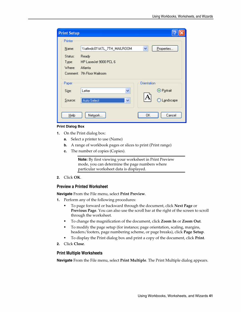
Using Workbooks, Worksheets, and Wizards
Using Workbooks, Worksheets, and Wizards 41
Print Dialog Box
1. On the Print dialog box: a. Select a printer to use (Name) b. A range of workbook pages or slices to print (Print range) c. The number of copies (Copies).
Note: By first viewing your worksheet in Print Preview mode, you can determine the page numbers where particular worksheet data is displayed.
2. Click OK.
Preview a Printed Worksheet
Navigate From the File menu, select Print Preview. 1. Perform any of the following procedures:
To page forward or backward through the document, click Next Page or Previous Page. You can also use the scroll bar at the right of the screen to scroll through the worksheet.
To change the magnification of the document, click Zoom In or Zoom Out. To modify the page setup (for instance; page orientation, scaling, margins,
headers/footers, page numbering scheme, or page breaks), click Page Setup. To display the Print dialog box and print a copy of the document, click Print.
2. Click Close.
Print Multiple Worksheets
Navigate From the File menu, select Print Multiple. The Print Multiple dialog appears.

Workbook and Worksheet Procedures
42 Oracle Retail Predictive Application Server
Print Multiple Dialog Box
1. Use Ctrl+Click to select multiple worksheets from the list provided. 2. Select Display print dialog before each window to have the Print Options dialog
displayed individually before each worksheet is printed. This feature allows you to specify different printing options for individual worksheets in the print queue. Deselect this option if the same printing options apply to all selected worksheets in the queue.
3. Click OK to submit your selections to the print queue. 4. Make your print option selections on the Print Options dialog. Selections made here
will apply to all printed worksheets if the Display print dialog before each window option is unchecked. If the option is checked, this dialog will appear before each worksheet is printed.
5. Click OK.
Format and Enhance Print Output There are several tools that you can use to enhance the output and the appearance of your printed worksheets. You can use these tools to generate custom reports from worksheets. Select Page Setup from the File menu to display printing options. Page Setup options always override any settings in the Windows Print Setup dialog box, and they only apply to the current document (worksheet or chart).
Change the Page Orientation
Note: To change page setup settings, you must display the data in Grid view (not Chart view).
Navigate From the File menu, select Page Setup. The Page Setup dialog appears.

Using Workbooks, Worksheets, and Wizards
Using Workbooks, Worksheets, and Wizards 43
Page Setup Dialog Box – Page Tab
1. On the Page tab, select the appropriate page orientation option, Portrait or Landscape.
2. Click OK.
Scale the Size of Printed Output
Note: To change page setup settings, you must display the data in Grid view (not Chart view).
Navigate From the File menu, select Page Setup. 1. In the Scaling portion of the Page tab, perform either one of the following
procedures: Click the Adjust To option and enter a numeric value between 10 and 400. This
is to specify an exact size for the printed output, which is a percentage of normal size.
Select the Fit To option to specify exact page parameters for the printed output. The system will automatically expand or condense the view so that the current slice fills the designated number of pages (height x width).
Note: You can leave one parameter blank (either height or width) to have the system fill pages along that dimension.
2. Click OK.

Workbook and Worksheet Procedures
44 Oracle Retail Predictive Application Server
Set Page Margins for Printed Documents
Note: To change page setup settings, you must display the data in Grid view (not Chart view).
Navigate From the File menu, select Page Setup. 1. Select the Margins tab. 2. Enter the desired values (in inches) for the top, bottom, left, and right margins.
Note: The combination of top and bottom margins must leave at least three inches of printable space per page.
3. View the results of your selections in the Preview window. 4. Click OK.
Create Customized Headers and Footers
Note: To change page setup settings, you must display the data in Grid view (not Chart view).
Navigate From the File menu, select Page Setup. 1. Select the Header/Footer tab. 2. Click the Custom Header or Custom Footer button. 3. Make changes to the left section, center section, and right section of the header or
footer by manually entering the text, or by selecting the following formatting buttons above the text window. Font – Opens the Font dialog where you specify the font, style, size, and script
type for your header and footer text. Select the header/footer text to be formatted, and click the Font button. On the Font dialog, make the appropriate selections. Click OK to apply the changes.
Date – Inserts a field marker code that prints the current date at the cursor position. This date is automatically updated each time you print the document. To insert a specific (unchanging) date, enter the date manually.
Time – Inserts a field marker code that prints the current time at the cursor position. The time is automatically updated each time you print the document. To insert a specific (unchanging) time, enter the time manually.
Page – Inserts a field marker code that prints the page number on each page of your document.
Page Of – Inserts a field marker code that prints the current page number and the total number of pages in the document at the cursor position. For example, 2 of 14.
Workbook – Inserts a field marker code that prints the current workbook title at the cursor position.
Sheet – Inserts a field marker code that prints the title of the current worksheet at the cursor position.
View – Inserts a field marker code that prints an actual worksheet view at the cursor position. Click this button to produce the Select Window dialog, which allows you to select the worksheet window to insert. The inserted window cannot be the same main worksheet for which you are specifying setup options. By adjusting page margins and scaling, you can use this functionality to

Using Workbooks, Worksheets, and Wizards
Using Workbooks, Worksheets, and Wizards 45
effectively print several worksheet views on a single page. Do this by inserting smaller windows into your header and footer.
4. Click the Save button to save this combination of header and footer options under a specified name.
5. Click OK to return to the Header/Footer dialog box to preview your work. 6. Click OK to close the Page Setup dialog.
Display Horizontal and Vertical Grid Lines on Printed Output
Note: To change page setup settings, you must display the data in Grid view (not Chart view).
Navigate From the File menu, select Page Setup. 1. Select the Sheet tab in the Page Setup window.
Page Setup Dialog Box – Margin Tab
2. In the Print section, make the appropriate selections as necessary: Select the Print Horizontal Grid Lines option to show horizontal grid lines. Select the Print Vertical Grid Lines option to show vertical grid lines.
3. Click OK.
Turn On/Off the Display of Hierarchy Tiles in Printed Output
Note: To change page setup settings, display the data in Grid view (not Chart view).

Workbook and Worksheet Procedures
46 Oracle Retail Predictive Application Server
Navigate From the File menu, select Page Setup. 1. Select the Sheet tab. 2. Select Print Hierarchy Tiles to turn on the display of hierarchy tiles in your output.
Deselect this option to turn off the display. 3. Click OK.
Display Row and Column Labels on Printed Output
Note: To change page setup settings, display the data in Grid view (not Chart view).
Navigate From the File menu, select Page Setup. 1. Select the Sheet tab. 2. In the Display Pages section, choose one of the following options:
Select All Pages to select row and column header labels to appear across the top and left side of every printed page.
Select Top & Left Pages to select row and column header labels to appear across the topmost and leftmost pages only. This is how they will appear on the terminal display.
3. Click OK.
Set the Page-Numbering Order
Note: To change page setup settings, display the data in Grid view (not Chart view).
Navigate From the File menu, select Page Setup. 1. Select the Sheet tab. 2. In the Page Order section, choose one of the following options:
Select Over, Then Down to select page numbering across sequential rows from left to right (starting in the upper left of the document).
Select Down, Then Over to select page numbering down sequential columns from top to bottom (starting in the upper left of the document).
3. Click OK.
Specify Page Breaks for Printed Output To change page setup settings, you must display the data in Grid view (not Chart view).
Specify Page Breaks after Each Position in a Selected Dimension You can specify that page breaks should occur in your printed output after every position in a given dimension. This ensures that you have a separate page of output for each month of data or a separate page for each subclass in the Product hierarchy.
Navigate From the File menu, select Page Setup. 1. Select the Page Breaks tab in the Page Setup window.
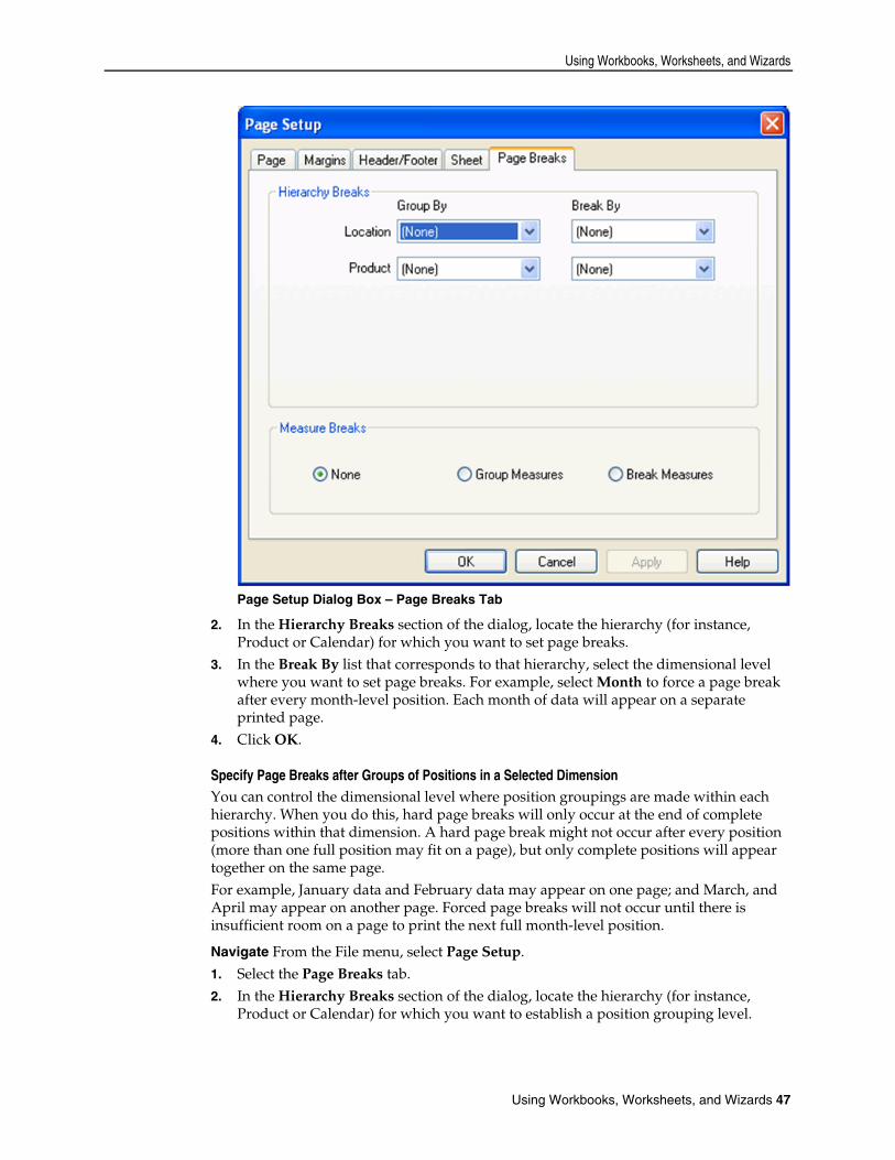
Using Workbooks, Worksheets, and Wizards
Using Workbooks, Worksheets, and Wizards 47
Page Setup Dialog Box – Page Breaks Tab
2. In the Hierarchy Breaks section of the dialog, locate the hierarchy (for instance, Product or Calendar) for which you want to set page breaks.
3. In the Break By list that corresponds to that hierarchy, select the dimensional level where you want to set page breaks. For example, select Month to force a page break after every month-level position. Each month of data will appear on a separate printed page.
4. Click OK.
Specify Page Breaks after Groups of Positions in a Selected Dimension You can control the dimensional level where position groupings are made within each hierarchy. When you do this, hard page breaks will only occur at the end of complete positions within that dimension. A hard page break might not occur after every position (more than one full position may fit on a page), but only complete positions will appear together on the same page. For example, January data and February data may appear on one page; and March, and April may appear on another page. Forced page breaks will not occur until there is insufficient room on a page to print the next full month-level position.
Navigate From the File menu, select Page Setup. 1. Select the Page Breaks tab. 2. In the Hierarchy Breaks section of the dialog, locate the hierarchy (for instance,
Product or Calendar) for which you want to establish a position grouping level.
Workbook and Worksheet Procedures
48 Oracle Retail Predictive Application Server
3. In the Group By list that corresponds to that hierarchy, select the dimensional level where you want to group positions. For example, select Month to force a page break after the maximum number of completed month positions have been fit onto a printed page.
4. Click OK.
Specify Page Breaks in the Measure Hierarchy The Measure hierarchy is treated separately from the other hierarchies, such as Calendar and Product since there is typically not a dimension level to specify when selecting page break options for measures. Follow these steps to specify page breaks in the Measure hierarchy:
Navigate From the File menu, select Page Setup. 1. Select the Page Breaks tab. 2. Click one of the following options in the Measure Breaks section of the dialog box:
None – There are no hard page breaks inserted in the printed output. This is the most economical option, because the maximum number of measures is fit onto each printed page.
Group Measures – This option inserts hard page breaks to be inserted whenever the maximum number of complete groups of measures has fit on a page.
Break Measures – This option inserts hard page breaks after every measure. Each measure will appear on a separate page of printed output.
3. Click OK.
Commit Changes to the Master Database The Commit process merges your local database with the master database. Therefore, your data is transferred to the master so all system users have access to the same data. There are two methods of committing data to the master – Commit Now and Commit Later. Commit Now immediately merges your workbook changes with the master database. When you select Commit Now, all other system users are temporarily locked out of the database during the commit process. The commit process requires that the master data file be overwritten, so no other users can build new workbooks or perform functions that require retrieval of data from the master file during this period. Whenever possible, you should select Commit Later to have your changes committed as part of an overnight batch process (when system use is minimal).
Commit a Workbook to the Master Database Immediately
Navigate From the File menu, select Commit Now. Click OK.
Commit a Workbook to the Master Database Later
Navigate From the File menu, select Commit Later. Click OK.
Note: A checkmark beside the Commit Later option on the File menu indicates that the workbook was flagged to be committed during the next batch process. To remove the workbook from the commit queue, select the Commit Later option again.
Using Workbooks, Worksheets, and Wizards
Using Workbooks, Worksheets, and Wizards 49
Working with Cells
Select and Manipulate Cells in a Grid Cells or groups of cells must be selected in the grid before certain operations can be performed on them. Operations, such as cutting and copying data, filling or clearing data cells, and displaying data in chart form are typically performed on a subset of worksheet cells that you must select before invoking the menu command. There are several ways to select cells in the grid. Generally, you should make your selections in the worksheet axes (where the column and row headers appear) and not in the cells themselves.
Select a Single Cell Click the column header that corresponds to the cell, and then click the corresponding row label.
Select all Cells in a Row Click the row header for that group of cells.
Select all Cells in a Column Click on the column header for that group of cells.
Select a Group of Continuous Cells in the Same Row 1. Click on the row header that corresponds to that group of cells. 2. Click on the column header for the first item in the group. 3. Hold down the Shift key, and click the column header that corresponds to the last
item in the group.
Select a Group of Continuous Cells in the Same Column 1. Click the column header that corresponds to that group of cells. 2. Click the row header for the first item in the group. 3. Hold down the Shift key, and click the row header that corresponds to the last item
in the group.
Select a Group of Non-Continuous Cells 1. Click the column header that corresponds to the first item in the group. 2. Hold down the Ctrl key, and click each column header that corresponds to a group
item. 3. Click the row header that corresponds to the first item in the group. 4. Hold down the Ctrl key, and click each row header that corresponds to a group item.
Select a Block of Contiguous Cells 1. Click the top-most, left-most cell in the block you want to select. 2. Hold down the mouse button and drag the cursor to the bottom-most, right-most cell
in the block that you want to select. As you drag the mouse, note that the column header and row header positions are automatically selected according to your actions.
3. Release the mouse button. 4. Click the row or column header to mark or unmark the last axis position selected.

Workbook and Worksheet Procedures
50 Oracle Retail Predictive Application Server
5. Press the spacebar to toggle the last axis position selection on and off.
Change a Cell's Size 1. Place the cursor on the cell border (either vertical line or horizontal line). 2. Click the left mouse button and drag the borderline until the cell size is the desired
width (or height).
Enter or Change Values in a Cell1 The following are descriptions of actions you can take to change individual values in a grid.
Numbers Enter or overwrite a numeric value.
Alphanumeric Values or Plain Text Enter or overwrite an alphanumeric value.
Drop-Down List Items Select the desired option from the drop-down list. Click on the arrow button and select an item from the drop-down list.
Date Items Select the desired date. Click the arrow button to display the calendar, and click the appropriate arrow keys to change the year, month, or date.
Check Box (Toggle) Items Click the check box to change the status of the item (yes or no, on or off).
Math Operations To increment the value in a cell using a mathematical formula, type in the following: To add – ‘+ [desired value to add]’ To subtract – ‘+- [desired value to subtract]’ To multiply – ‘* [desired value to multiply by]’ To divide – ‘/ [desired value to divide by]’ To apply a percentage – ‘* [desired percentage increment]’ (For example, to increase a
value by one-half, enter * 1.5.)
Modify Data with Cell Formulas1 Cell formulas allow you to modify the value of a data cell in the grid by applying an operator (+, -, *, or /) to that value. With this functionality, you can make changes to data values without having to manually calculate the result. To perform this function, click in the data cell and type the operator that you want to add, subtract, multiply, or divide by. For example, suppose that a particular data cell contains the value 10. Add – If you enter +10 in the cell, the value becomes 20. Subtract – If you enter + –10 in the cell, the value becomes 0. Multiply – If you enter *10 in the cell, the value becomes 100. Divide – If you enter /10 in the cell, the value becomes 1.
Using Workbooks, Worksheets, and Wizards
Using Workbooks, Worksheets, and Wizards 51
Percentages – If you want to increase the value of a cell by 10%, multiply the value by 1.1 (enter *1.1)
There are many applications of cell formulas when modifying data. Cell formulas can only be applied to one cell at a time, but changes made to aggregate level cells will be spread down to lower-level cells along hierarchy lines. Similarly, any changes made to lower level cells will be reflected in the aggregates of that data.
Clear and Fill Cells in a Worksheet1 Use the following procedures to clear data from worksheet cells and to quickly populate the cells of a worksheet.
Clear Data from Cells 1. Select the data cells that you want to clear.
Note: If you do not select any data cells before you choose Clear Contents, in the next step, the system will clear the data cells for every writable measure in the currently-displayed slice. If you select certain cells; however, only those cells will be cleared.
2. From the Edit menu, select Clear Contents.
Note: You can only clear contents from one dimensional level at a time. If you are viewing data in Outline mode, the Clear Contents dialog requires you to specify the dimension that you want cleared.
3. Click OK.
Fill (Populate) the Cells of a Worksheet Use this procedure to quickly populate cells in a worksheet with a single value. This command only fills cells in one measure at a time. 1. Select the cells in the grid to be filled.
Note: If you do not select any data cells before using the Fill command; in the next step, the system will fill the cells for an entire measure. If you select certain data cells, only those selected cells will be filled.
2. From the Edit menu, select Fill. 3. Select the measure to be filled from the Measure list. 4. Specify a fill value in the Fill Value field. 5. If you are filling data at a level other than base level, select a Spread Method
(Replicate, Even, Proportional, or Delta). 6. If you are viewing data in Outline mode, the bottom portion of the Fill dialog
requires you to specify the dimensional level at which to fill data. The system can only fill data for cells in one dimension at a time.
7. Click OK.
Cut and Copy the Data in Worksheet Cells
Cut the Contents of Worksheet Cells

Workbook and Worksheet Procedures
52 Oracle Retail Predictive Application Server
Use this procedure to copy selected data to the application clipboard and to clear that data from the worksheet cells. Only data from writable measures can be cut. This procedure cuts data at the current hierarchical level, which is the lowest level that data is selected in the grid. 1. Select all data cells in the grid that you want to cut. If you do not select any data cells
before using the Cut command, the following error message appears.
If you select specific data cells, only the data for those cells will be cut. 2. From the Edit menu, select Cut, or click the Cut button on the application toolbar.
Copy the Contents in Worksheet Cells Use this procedure to copy selected data to the application clipboard. Unlike the Cut function, the Copy function does not clear the data from the worksheet cells. This procedure copies data at the current hierarchical level, which is the lowest level that data is selected in the grid.
Note: Any cells affected by deferred calculations must be either calculated or discarded by the user before the cells can be copied to the clipboard.
1. Select all data cells in the grid that you want to copy. If you do not select any data cells before using the Copy command, the dialog (above) is displayed. If you select specific data cells, only the data for those cells will be copied.
2. From the Edit menu, select Copy, or click the Copy button on the application toolbar.
Note: The copy and paste operation for aggregated measures with ambiguous (ambig) measure types is not supported. However, "copy at base" works for ambig measures at aggregated levels.
Paste Copied Data into Cells Use this procedure to paste data into measures. This procedure can only be performed if data has been placed on the application clipboard using a cut or copy function. Data can only be pasted into writable measures.
Cut or Copy Data to Paste into Other Cells 1. Select the data cells where you want the data pasted into. Only those selected cells
will be overwritten with the pasted data. 2. From the Edit menu; select Paste, or click the Paste button on the application toolbar.
Cut, Copy, and Paste Base-Level Data You can cut, copy, and paste data at the base level in your worksheet while viewing it at any aggregate level. Cutting, copying, and pasting in this manner allows you to quickly make base level changes by manipulating data at an aggregate level.

Using Workbooks, Worksheets, and Wizards
Using Workbooks, Worksheets, and Wizards 53
You choose whether or not to perform operations on base level data by manipulating the appropriate check box that appears on the Cut Special, Copy Special, and Paste Special dialog boxes.
Cut Base-Level Data The cut data at base level feature allows you to view data at an aggregate level in your worksheet while cutting that same data at its base dimensional level, which is not currently displayed. When you select the Cut Special function at an aggregate level, and you select the Cut Data at Base Level check box (on the Cut Special dialog); all base level data applicable to your selected aggregate data will be cut and copied to the application clipboard. Even though the Cut function is performed at the base dimensional level, it seems that the aggregate level data has been cut. This is due to the process of data roll-up. To use the cut data at base level functionality, the base dimensional level for a given hierarchy cannot be displayed in your worksheet if you are in block view. 1. Select the aggregate level data to be cut. Only data from writable measures can be
cut.
Note: If your grid data contains any measures that are read-only, the system will be unable to cut data for the entire worksheet. In this case, a message will inform you that the cut request could not be completed.
2. From the Edit menu, select Cut Special. 3. Select the Cut Data at Base Level check box. Selecting the base level cut option
causes all base level data applicable to your aggregate selection to be cut and copied to the application clipboard.
4. Click OK.
Copy Base-Level Data The copy data at base level feature allows you to view data at an aggregate level in your worksheet while copying that same data at its base dimensional level, which is not currently displayed. When you select the Copy Special function at an aggregate level, and you check the Copy Data at Base Level checkbox (on the Copy Special dialog), all base level data that is applicable to your selected aggregate data will be copied to the clipboard. Unlike the Cut Special function, Copy Special does not clear the data from the copied cells. Even though the Copy Special function is actually performed at the base dimensional level; after pasting, it seems like the aggregate level data has been copied. This is due to the process of data roll-up. To use the copy data at base level functionality, the base dimensional level for a given hierarchy cannot be displayed in your worksheet. 1. Select the aggregate level data to be copied.
Note: If no data cells are selected in the grid at the time the Copy Special dialog is opened, the system displays a dialog stating there are not any positions selected for the operation.
2. From the Edit menu, select Copy Special.

Workbook and Worksheet Procedures
54 Oracle Retail Predictive Application Server
3. Select the Copy Data at Base Level option. Selecting the base level copy option causes all base level data applicable to your aggregate selection to be copied to the application clipboard.
4. Click OK.
Paste Base-Level Data The paste data at base level feature allows you to view data at an aggregate level in your worksheet while pasting data into measures at the base dimensional level, which is not currently displayed. The Paste Special menu item is only enabled after you place information on the application clipboard using the Cut, Cut Special, Copy, or Copy Special command. When you select the Paste Special function at an aggregate level, and you select the Paste Data at Base Level checkbox (on the Paste Special dialog), data will be pasted into the base level cells associated with your aggregate level paste selection. To use the paste data at base level functionality, the base dimensional level for a given hierarchy cannot be displayed in your worksheet. To paste data at base level, ensure that you are viewing values at an aggregate level only, and perform the following steps: 1. Select the aggregate level cells that you want to paste the cut/copied data into. Only
those cells will be overwritten with pasted data. You can only paste data into writable measures.
2. From the Edit menu, select Paste Special. 3. Ensure that the Paste Data at Base Level checkbox is selected. Whenever data has
just been cut or copied at base level, the Paste Data at Base Level checkbox defaults to selected.
4. Click OK.
Cut, Copy, and Paste Multiple Slices When you make cell selections prior to cutting, copying, or pasting data; the system only allows for the selection of the currently displayed position along the slice axis. The Cut Special, Copy Special, and Paste Special dialog boxes; however, allow you to specify that data should be manipulated for all positions (pages) in this axis.
Copy Data from All Slices Use this procedure to simultaneously copy data from all pages in the slice axis. 1. Select the data cells to be copied. 2. From the Edit menu, select Copy Special. 3. On the Copy Special dialog, select Copy All Slices. When the box is selected, the
copy operation behaves as if all positions in the slice dimension were selected prior to the copy. If the box is not selected, only data from the currently displayed slice position will be copied.
4. Click OK.
Cut Data from All Slices Use this procedure to cut data from all pages in the slice axis simultaneously. 1. Select the data cells to be cut. 2. From the Edit menu, select Cut Special. 3. On the Cut Special dialog, select Cut All Slices. When the box is selected, the cut
operation behaves as if all positions in the slice dimension were selected prior to the

Using Workbooks, Worksheets, and Wizards
Using Workbooks, Worksheets, and Wizards 55
cut. If the option is not selected, only data from the currently displayed slice position will be cut.
4. Click OK.
Paste Data into All Slices Use this procedure to simultaneously paste data into all pages in the slice axis.
Note: You can only paste data into writable measures.
1. Select the cells where you want to paste the cut/copied data. Only those cells will be overwritten with the pasted data.
2. From the Edit menu, select Paste Special. 3. On the Paste Special dialog, select Paste All Slices. When the box is checked, the
paste operation behaves as if all positions in the slice dimension were selected prior to the paste. If the box is unchecked, data will only be pasted into the currently displayed slice position.
Note: If you did not choose to cut/copy data from all slices prior to this paste, and then you choose to paste clipboard data to all slices, the data that was cut/copied from the single visible slice will be replicated to all slices in the worksheet.
4. Click OK.
Copy Data to and Paste Data from the Windows Clipboard1 The Cut, Cut Special, Copy, and Copy Special commands do not copy information to the Windows clipboard. When you use these functions, data is copied to an application-specific clipboard and cannot be pasted into other applications. If you plan on pasting worksheet data into another application, or if you want to paste data from another application into your worksheet, you must use the following procedures.
Copy Data to the Windows Clipboard Use this procedure if you want to copy worksheet data to use in another application. 1. Select the data cells whose contents are to be copied. 2. From the Edit menu, select Copy to Clipboard.
Note: When using this command, the maximum number of cells that can be copied is limited by memory. This operation should not be used to export entire workbooks.
Paste Data from the Windows Clipboard into a Worksheet Use this procedure if you want to paste data from the Windows clipboard into your worksheet. Data can only be pasted into writable measures. 1. Select the data cells where you want to paste the clipboard data. 2. From the Edit menu, select Paste from Clipboard.
Note: When using this command, the maximum number of cells that can be pasted is limited by memory. This operation should not be used to import data for entire workbooks.
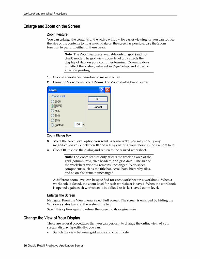
Workbook and Worksheet Procedures
56 Oracle Retail Predictive Application Server
Enlarge and Zoom on the Screen
Zoom Feature You can enlarge the contents of the active window for easier viewing, or you can reduce the size of the contents to fit as much data on the screen as possible. Use the Zoom function to perform either of these tasks.
Note: The Zoom feature is available only in grid (and not chart) mode. The grid view zoom level only affects the display of data on your computer terminal. Zooming does not affect the scaling value set in Page Setup, and it has no effect on printing.
1. Click in a worksheet window to make it active. 2. From the View menu, select Zoom. The Zoom dialog box displays.
Zoom Dialog Box
3. Select the zoom level option you want. Alternatively, you may specify any magnification value between 10 and 400 by entering your choice in the Custom field.
4. Click OK to close the dialog and return to the resized worksheet.
Note: The Zoom feature only affects the working area of the grid (column, row, slice headers, and grid data). The size of the worksheet window remains unchanged. Worksheet components such as the title bar, scroll bars, hierarchy tiles, and so on also remain unchanged.
A different zoom level can be specified for each worksheet in a workbook. When a workbook is closed, the zoom level for each worksheet is saved. When the workbook is opened again, each worksheet is initialized to its last saved zoom level.
Enlarge the Screen Navigate: From the View menu, select Full Screen. The screen is enlarged by hiding the Windows status bar and the system title bar. Select this option again to return the screen to its original size.
Change the View of Your Display There are several procedures that you can perform to change the online view of your system display. Specifically, you can: Switch the view between grid mode and chart mode
Using Workbooks, Worksheets, and Wizards
Using Workbooks, Worksheets, and Wizards 57
Show or hide various screen components Invoke the zooming feature to alter the size of the grid contents
Change Charts to Grids and Back
Change a Grid to a Chart Use this procedure to display some or all of the data from a grid in a chart view. You can display up to 1000 positions of data in chart view. 1. To select specific data to appear in chart form, highlight all cells that you want to see
displayed, or to display all of the grid’s data on a chart, do not select any data.
2. From the View menu, select Chart, or select the button on the toolbar.
Note: Chart view (especially line charts) is often used to easily identify trends and changes in data over periods of time. When you use a chart for this purpose, position the Calendar hierarchy tile along the column axis, and position the Measure hierarchy tile along the row axis. This will extend the time dimension along the x-axis and extend the measure of interest (such as Total Sales or Forecasted Demand) along the y-axis. You can position the Product and Location hierarchy tiles wherever you wish, such as along the slice-axis (z-axis) or alongside the Measure tile (row, or y-axis).
Change a Chart to a Grid
Navigate From the View menu, select Grid, or select the button on the toolbar.
Show and Hide the Button Text, Status Bar, and Toolbar
Show/Hide Button Text in the Application Toolbar Follow this procedure to turn on/off the display of toolbar button names in the application toolbar.
Navigate From the Format menu, select Application. 1. Under Application Options, select the Show Button Text option to display button
names on the application toolbar. Clear this option to turn off the display of button titles.
2. To apply the change to the worksheet without closing the dialog box, click Apply, or to accept the change and close the Format Options dialog, click OK.
Show/Hide Status Bar
Navigate From the View menu, select Status Bar. Select Status Bar again to re-display it.
Show/Hide Toolbar
Navigate From the View menu, select Toolbar. Select Toolbar again to re-display it.

Workbook and Worksheet Procedures
58 Oracle Retail Predictive Application Server
Enter Measure Data Using a Scaling Factor The scaling factor feature allows you to enter measure data that will be scaled or factored to an internal value, which is recognized by the server in data calculations. When you enter a value for a measure that has a scaling factor, the value that you enter will be multiplied by the scaling factor to arrive at this internal value. The display of the data and the ease of data entry can be greatly enhanced by use of a scaling factor. For example, suppose that you want to enter data in thousands of units. You might find it tedious to enter 1000, 2000, 6000, and so on. A more sensible approach would be to enter the values 1, 2, and 6, and have the system apply a scaling factor (in this case 1000) to the entered data. The internal values of the three affected cells would be 1000, 2000, and 6000, and these internal values would be used in required data calculations. Removing the zeros from the display would result in a cleaner, less cumbersome worksheet appearance. The scaling factor feature is used in conjunction with the prefix/suffix feature for formatted measures. In the case above, you would probably want to specify a suffix (for instance, k stands for 1000) for this measure, which indicates that the entered data has been scaled. The displayed data would then appear as 1k, 2k, and 6k. Even though your worksheet has been "cleaned up" by abbreviating the numeric display, the system still understands that the internal values of the edited cells are 1000, 2000, and 6000, respectively.
Specify a Scaling Factor for a Measure
Navigate From the Format menu, select Types.
Format Options Dialog Box – Types Tab
1. In the Measure box, select the measure that you want to edit.
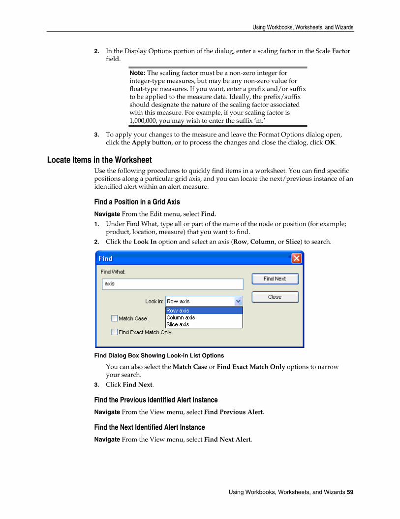
Using Workbooks, Worksheets, and Wizards
Using Workbooks, Worksheets, and Wizards 59
2. In the Display Options portion of the dialog, enter a scaling factor in the Scale Factor field.
Note: The scaling factor must be a non-zero integer for integer-type measures, but may be any non-zero value for float-type measures. If you want, enter a prefix and/or suffix to be applied to the measure data. Ideally, the prefix/suffix should designate the nature of the scaling factor associated with this measure. For example, if your scaling factor is 1,000,000, you may wish to enter the suffix ‘m.’
3. To apply your changes to the measure and leave the Format Options dialog open, click the Apply button, or to process the changes and close the dialog, click OK.
Locate Items in the Worksheet Use the following procedures to quickly find items in a worksheet. You can find specific positions along a particular grid axis, and you can locate the next/previous instance of an identified alert within an alert measure.
Find a Position in a Grid Axis
Navigate From the Edit menu, select Find. 1. Under Find What, type all or part of the name of the node or position (for example;
product, location, measure) that you want to find. 2. Click the Look In option and select an axis (Row, Column, or Slice) to search.
Find Dialog Box Showing Look-in List Options
You can also select the Match Case or Find Exact Match Only options to narrow your search.
3. Click Find Next.
Find the Previous Identified Alert Instance
Navigate From the View menu, select Find Previous Alert.
Find the Next Identified Alert Instance
Navigate From the View menu, select Find Next Alert.

Workbook and Worksheet Procedures
60 Oracle Retail Predictive Application Server
Rotate or Pivot an Axis on a Grid Rotating or pivoting an axis (such as product, time, or location) on a grid allows you to display data in different orientations.
To Pivot along the Same Axis 1. Left-click and hold the hierarchy tile representing the hierarchy that you want to
move. 2. Drag the hierarchy tile to the desired new position along the axis. 3. Observe the appearance of the cursor as you move the tile. When the cursor is over
an available dropping point (display area), its appearance will change. 4. To drop the tile in its new display area, release the mouse button.
To Rotate a Hierarchy to Another Axis 1. Left-click on and hold the hierarchy tile representing the hierarchy that you want to
move. 2. Drag the hierarchy tile to the desired display axis. 3. Observe the appearance of the cursor as you move the tile. When the cursor is over
an available dropping point (display area), its appearance changes into an arrow. 4. To drop the tile in its new display area, release the mouse button.
Show and Hide Positions in the Grid Display Once you have created a workbook that contains the products, time periods, and measures selected in the workbook wizard; you are able to hide any positions (nodes) that were initially incorporated during the workbook build. The position hiding feature allows you to remove undesired information from the grid display without requiring you to rebuild the workbook to attain the view you want.
Note: When you select individual positions to hide from view, any data associated with those hidden nodes will still be reflected in any aggregate totals.
Hide Positions using the Quick Menu 1. Select an undesired node by clicking it within the axis display.
Note: Use Ctrl+Click to select multiple positions together.
2. Right-click the mouse within that same axis area to produce the associated quick menu.
3. Choose Hide Selection.
Hide Positions using the Show/Hide Dialog One method of hiding positions in the grid display is to access the Show/Hide dialog, which is actually the Show/Hide tab of the Tree Options dialog. This method is useful if you have a large number of nodes to hide at the same time. The Show/Hide dialog also provides the means to return already hidden nodes to the grid display.
Note: The following procedure is used to show positions in hierarchies other than the Measure hierarchy.
Using Workbooks, Worksheets, and Wizards
Using Workbooks, Worksheets, and Wizards 61
1. Right-click in a dimension’s axis area to display the quick menu relevant to that hierarchy.
2. Select Show/Hide. When the Show/Hide dialog displays, all currently hidden nodes are displayed on the left side of the dialog, and all currently visible nodes are displayed on the right side.
3. Click a node on the right side of the dialog to select it. Use Ctrl+Click to select multiple nodes together.
4. Click the left arrow button to move your selection(s) to the Hidden Nodes side of the dialog.
5. Click OK. When you return to the workbook, the grid display reflects the selections made on the Show/Hide tab.
Note: Any data associated with the hidden position(s) will still be reflected in any aggregate totals.
Re-display Currently Hidden Positions The Show/Hide dialog provides the means to make any hidden positions visible in the grid display. Perform the steps below to re-display hidden positions in the grid.
Note: The following procedure is used to show positions in hierarchies other than the Measure hierarchy.
1. Right-click in a dimension’s axis area to display the quick menu relevant to that hierarchy.
2. Select Show/Hide. When the dialog displays, all currently hidden nodes are displayed on the left side of the screen and all currently visible nodes are displayed on the right side.
3. Click a node on the left side of the screen to select it. Use Ctrl+Click to select multiple nodes together.
4. Click the right arrow button to move your selection(s) to the Visible Nodes side. 5. Click OK.
When you return to the workbook, the grid display reflects the selections made on the Show/Hide tab.
Show and Hide Positions in the Measure Hierarchy Measure positions can be hidden from view in the same way as positions in other hierarchies. However, the Show/Hide dialog for measures appears much different. The Show/Hide Measures dialog has been designed to streamline the selection of measures, taking into account the attributes that comprise each measure’s definition.
Hide Currently Visible Measures from View To use the Show/Hide Measures dialog to hide a visible measure from grid view, perform the following steps: 1. On a worksheet, right-click in the measure axis to produce the associated quick
menu. 2. Select Show/Hide.
Workbook and Worksheet Procedures
62 Oracle Retail Predictive Application Server
3. In the Visible Measures portion of the dialog (upper right), click on a measure that you want to hide. You may select multiple measures from this list by using Ctrl+Click.
4. Click the left arrow button. The selected measures are removed from the Visible Measures window.
5. Click OK.
Show Hidden Measures in the Grid Display To use the Show/Hide Measures dialog to return a hidden measure to the grid display, perform the steps below.
Note: For most selections made in the following steps, multiple selections can be made by using Ctrl+Click.
1. On a worksheet, right-click in the measure axis to produce the associated quick menu.
2. Select Show/Hide. 3. In the Hidden Measures portion of the dialog, select the measures you want to hide. 4. Click the right arrow button to add the measure to the Visible Measures list. 5. Click OK.
Specify the Display Order of Measures in the Grid You can use the Show/Hide Measures dialog to specify or change the order in which measures are displayed in the grid. To do this, perform the following steps: 1. On a worksheet, right-click in the measure axis to produce the associated quick
menu. 2. Select Show/Hide. 3. Select a measure from the Visible Measures list. 4. Click the up arrow or down arrow to move the selected measure up or down in the
list display. 5. Repeat these steps for measures as required until the appropriate display order is
attained. 6. Click OK.
Measure Profiles
Create a Measure Profile 1. On a worksheet, right-click in the measure axis to produce the associated quick
menu. 2. Select Show/Hide. 3. Select all of the measures that you want to include in the measure profile, and ensure
that all desired measures appear in the Visible Measures window. In the Measure Profiles text field, type a name for the profile.
4. Click Add Profile to save the list. 5. Click OK.
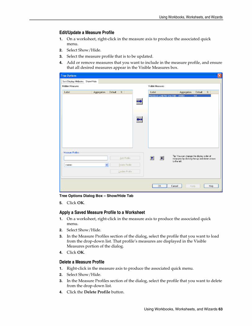
Using Workbooks, Worksheets, and Wizards
Using Workbooks, Worksheets, and Wizards 63
Edit/Update a Measure Profile 1. On a worksheet, right-click in the measure axis to produce the associated quick
menu. 2. Select Show/Hide. 3. Select the measure profile that is to be updated. 4. Add or remove measures that you want to include in the measure profile, and ensure
that all desired measures appear in the Visible Measures box.
Tree Options Dialog Box – Show/Hide Tab
5. Click OK.
Apply a Saved Measure Profile to a Worksheet 1. On a worksheet, right-click in the measure axis to produce the associated quick
menu. 2. Select Show/Hide. 3. In the Measure Profiles section of the dialog, select the profile that you want to load
from the drop-down list. That profile’s measures are displayed in the Visible Measures portion of the dialog.
4. Click OK.
Delete a Measure Profile 1. Right-click in the measure axis to produce the associated quick menu. 2. Select Show/Hide. 3. In the Measure Profiles section of the dialog, select the profile that you want to delete
from the drop-down list. 4. Click the Delete Profile button.
Workbook and Worksheet Procedures
64 Oracle Retail Predictive Application Server
5. Click OK to return to the workbook. 6. In the Measure Profiles text field, type the same name for the profile that is to be
updated. 7. Click OK.
Select a Higher Hierarchy Level for Data Roll-Up 1. Right-click on the desired grid axis. 2. Left-click and select Select Rollup. 3. Select the highest dimension to display.
Aggregate Data
Aggregate Data Using a Dimension List The Dimension List option allows you to collapse/expand the display of one dimension at a time. When a worksheet dimension is collapsed from the grid display, all of that dimension’s associated data is aggregated to the next higher level currently displayed. 1. Right-click any worksheet axis to display a quick menu of options that are relevant to
that hierarchy. Dimensions that are currently displayed are shown in the dimension list with checkmarks beside them.
Note: If you want to aggregate data to a dimension higher than those shown in the dimension list, you must first use the Select Rollup option to specify the highest dimension that you want to see.
2. Click any currently checked dimension to collapse that hierarchical level. All associated data will be aggregated to the next higher dimension that is displayed.
Note: When you click any unchecked dimension in the list, the reverse process happens. The previously collapsed dimension will be displayed in the grid in its proper relative location in the hierarchy.
Aggregate Data using the Select Dimensions Menu The Select Dimensions option allows you to collapse or expand the display of multiple dimensions at one time. Select this option to display a dialog box in which you can select exactly which dimensions you would like displayed in your worksheet. 1. Right-click any worksheet axis to display a quick menu of options that are relevant to
that hierarchy. 2. Select Select Dimensions. 3. On the dialog that opens, select all dimensions that you want to display in your
worksheet. Highlighted dimensions will appear in the display. Non-highlighted dimensions will be collapsed and data will be aggregated to the next higher level.
Note: If you want to select a dimension higher than those shown in the dimension list, use the Select Rollup option to specify the highest dimension you want to see.
4. Click OK.
Using Workbooks, Worksheets, and Wizards
Using Workbooks, Worksheets, and Wizards 65
Aggregate Data Using the Dimension Labels The Show Dimension Labels option is useful when you need to repeatedly collapse/expand dimensions without having to access the quick menu every time you do it. This option toggles the display of cursor-sensitive dimension header labels in your worksheet. When you click the label for a particular dimension, that dimension is collapsed in the grid and all associated data is aggregated to the next higher level. Once the dimension header labels are activated, dimensions can be collapsed or expanded with a single click the mouse. 1. Right-click on any worksheet axis to display a quick menu of options relevant to that
hierarchy. 2. Select the Show Dimension Labels option.
Note: Minimized tabs are displayed at the left side of the column axis headings or at the top of the row axis headings. This depends on your axis selection.
3. Place the cursor over these tabs. The tabs expand to display the dimension labels. 4. Click on any dimension label to collapse that dimension in the grid and aggregate the
data to the next higher level.
Note: Labels representing collapsed dimensions contain only a plus (+) sign. Click on the plus sign to maximize the label and expand that dimension in the grid.
Spread Aggregate Data from an Individual Cell 1. Click inside an aggregate-level cell to edit. Spreading is ineffective for base-level
(lowest-level) data. 2. In the cell, type a numeric value followed by one of the following:
r (replicate) e (even) d (delta) p (proportional)
The values will use your spread method choice to spread to the lowest level. For a description of the spreading methods, see the Spreading overview topic.
Spread Aggregate Data from Many Cells Select an aggregate-level cell or a group of aggregate-level cells that you want to contain the same value.
Navigate From the Edit menu, select Fill. 1. Click the arrow below Measure, and select the measure that you want to fill. If you
selected cells in the grid before selecting Fill, only the selected cells will be filled. If you did not select any cells, all of the cells for the measure selected will be filled.
2. In the Fill Value field, type a fill value. If the measure type is numeric, make sure that the value entered is numeric, and go to step 5. If the measure type is non-numeric (can only contain values from a list), select the desired value from the drop-down list, and go to step 6.

Workbook and Worksheet Procedures
66 Oracle Retail Predictive Application Server
Note: If you are viewing data in Outline mode when you select the Fill command, the system requires you to specify the aggregate level where you want to fill data. If the dimension you select is not an aggregate level, the Spread Method functions on the Fill dialog box will be disabled.
3. Select Spread Method (Replicate, Even, Delta, or Proportional). See the Spreading overview topic for a description of the spreading methods.
4. Click OK.
Dimension and Sorting Attributes
Overview RPAS supports user definition of attributes on-the-fly within the workbook. The Attribute Definition feature allows dimension attributes to be created, deleted or modified. Such attributes are referred to as “dynamic dimension attributes”, as opposed to “static dimension attributes” that are registered to the domain by RPAS “dattrmgr” utility (see the RPAS Administration Guide for more information on the registration of static dimension attributes). During workbook build process, dynamic dimension attributes are brought into the workbook by RPAS framework if the dimension is present and the following conditions are met: The attribute is accessible by the log-on user. The source measure exists in the workbook. The other positions of this attribute fits into the workbook context.
The dynamic dimension attributes can be used for dimension splitting, sorting and displaying in the workbook. The attribute data is only updated when the attribute is used. Dynamic Dimension Attributes are excluded from the Extra Measure Page and Insert Measure menu option, because their representing measures have the “insertable” field set to false.
Adding a New Dynamic Attribute
Navigate Right-click over the hierarchy tile or positions in which to apply the new attribute, select the Attribute definition menu. From this menu the user can view the Attribute Address Selections dialog box. 1. The Select Attribute Dimension box defaults to hierarchy and dimension in which the
user initiated the Attribute definition window. You may change the dimension or the hierarchy to apply the attribute. If the hierarchy is modified, the click Select to reset the default values in the Select Source Measure and Select Other Hierarchies boxes. In the example below, positions along the Store dimension will have the resulting attribute applied.
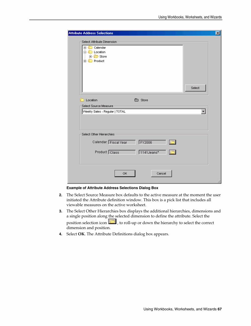
Using Workbooks, Worksheets, and Wizards
Using Workbooks, Worksheets, and Wizards 67
Example of Attribute Address Selections Dialog Box
2. The Select Source Measure box defaults to the active measure at the moment the user initiated the Attribute definition window. This box is a pick list that includes all viewable measures on the active worksheet.
3. The Select Other Hierarchies box displays the additional hierarchies, dimensions and a single position along the selected dimension to define the attribute. Select the
position selection icon , to roll-up or down the hierarchy to select the correct dimension and position.
4. Select OK. The Attribute Definitions dialog box appears.

Workbook and Worksheet Procedures
68 Oracle Retail Predictive Application Server
Attribute Definitions Dialog Box
5. From the Available Attributes drop-down list, select from the list of existing attributes, or click New if a new attribute is to be defined. If an existing attribute is selected from the drop-down list and it was previously defined using the Attribute Definitions dialog box, the values in the dialog default to the selections previously assigned to this attribute. You can modify any of these values.
6. Select the appropriate Band Type options, which determine whether or not the positions to which the attribute will be assigned are clustered. Select No Clustering if the measure data is to be used as an attribute label. Select Clustering if positions are to be grouped based on attribute values, enter
the number of clusters (range is 1 to 100) in the Clustering text field, and click Create Clusters. The Clustering Input area of the screen displays new fields and information. The Clustering Input area displays the same number of cluster labels as the number of clusters defined in the Clustering text field.
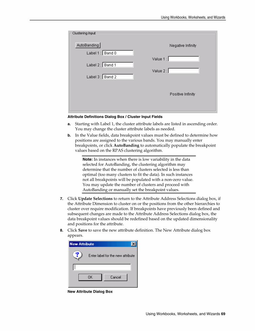
Using Workbooks, Worksheets, and Wizards
Using Workbooks, Worksheets, and Wizards 69
Attribute Definitions Dialog Box / Cluster Input Fields
a. Starting with Label 1, the cluster attribute labels are listed in ascending order. You may change the cluster attribute labels as needed.
b. In the Value fields, data breakpoint values must be defined to determine how positions are assigned to the various bands. You may manually enter breakpoints, or click AutoBanding to automatically populate the breakpoint values based on the RPAS clustering algorithm.
Note: In instances when there is low variability in the data selected for AutoBanding, the clustering algorithm may determine that the number of clusters selected is less than optimal (too many clusters to fit the data). In such instances not all breakpoints will be populated with a non-zero value. You may update the number of clusters and proceed with AutoBanding or manually set the breakpoint values.
7. Click Update Selections to return to the Attribute Address Selections dialog box, if the Attribute Dimension to cluster on or the positions from the other hierarchies to cluster over require modification. If breakpoints have previously been defined and subsequent changes are made to the Attribute Address Selections dialog box, the data breakpoint values should be redefined based on the updated dimensionality and positions for the attribute.
8. Click Save to save the new attribute definition. The New Attribute dialog box appears.
New Attribute Dialog Box
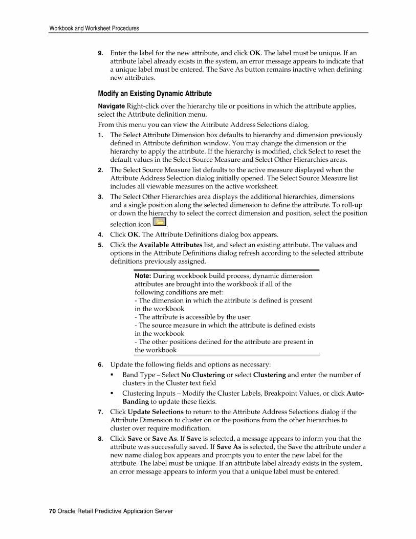
Workbook and Worksheet Procedures
70 Oracle Retail Predictive Application Server
9. Enter the label for the new attribute, and click OK. The label must be unique. If an attribute label already exists in the system, an error message appears to indicate that a unique label must be entered. The Save As button remains inactive when defining new attributes.
Modify an Existing Dynamic Attribute
Navigate Right-click over the hierarchy tile or positions in which the attribute applies, select the Attribute definition menu. From this menu you can view the Attribute Address Selections dialog. 1. The Select Attribute Dimension box defaults to hierarchy and dimension previously
defined in Attribute definition window. You may change the dimension or the hierarchy to apply the attribute. If the hierarchy is modified, click Select to reset the default values in the Select Source Measure and Select Other Hierarchies areas.
2. The Select Source Measure list defaults to the active measure displayed when the Attribute Address Selection dialog initially opened. The Select Source Measure list includes all viewable measures on the active worksheet.
3. The Select Other Hierarchies area displays the additional hierarchies, dimensions and a single position along the selected dimension to define the attribute. To roll-up or down the hierarchy to select the correct dimension and position, select the position
selection icon . 4. Click OK. The Attribute Definitions dialog box appears. 5. Click the Available Attributes list, and select an existing attribute. The values and
options in the Attribute Definitions dialog refresh according to the selected attribute definitions previously assigned.
Note: During workbook build process, dynamic dimension attributes are brought into the workbook if all of the following conditions are met: - The dimension in which the attribute is defined is present in the workbook - The attribute is accessible by the user - The source measure in which the attribute is defined exists in the workbook - The other positions defined for the attribute are present in the workbook
6. Update the following fields and options as necessary: Band Type – Select No Clustering or select Clustering and enter the number of
clusters in the Cluster text field Clustering Inputs – Modify the Cluster Labels, Breakpoint Values, or click Auto-
Banding to update these fields. 7. Click Update Selections to return to the Attribute Address Selections dialog if the
Attribute Dimension to cluster on or the positions from the other hierarchies to cluster over require modification.
8. Click Save or Save As. If Save is selected, a message appears to inform you that the attribute was successfully saved. If Save As is selected, the Save the attribute under a new name dialog box appears and prompts you to enter the new label for the attribute. The label must be unique. If an attribute label already exists in the system, an error message appears to inform you that a unique label must be entered.

Using Workbooks, Worksheets, and Wizards
Using Workbooks, Worksheets, and Wizards 71
Delete an Existing Dynamic Attribute
Navigate Right-click over the hierarchy tile or positions in which the attribute applies, select the Attribute definition menu. From this menu you can view the Attribute Address Selections dialog. 1. The Select Attribute Dimension box defaults to hierarchy and dimension previously
defined in Attribute definition window. You may change the dimension or the hierarchy to apply the attribute. If the hierarchy is modified, click Select to reset the default values in the Select Source Measure and Select Other Hierarchies areas.
2. The Select Source Measure list defaults to the active measure displayed when the Attribute Address Selection dialog initially opened. The Select Source Measure list includes all viewable measures on the active worksheet.
3. The Select Other Hierarchies area displays the additional hierarchies, dimensions and a single position along the selected dimension to define the attribute. To roll-up or down the hierarchy to select the correct dimension and position, select the position
selection icon . 4. Click OK. The Attribute Definitions dialog box appears. 5. Click the Available Attributes list, and select an existing attribute. The values and
options in the Attribute Definitions dialog refresh according to the selected attribute definitions previously assigned.
6. Click Delete to remove the attribute definition from the system. A message appears to inform you that the attribute was successfully deleted.
7. Click Exit to close the Attribute Definition dialog box.
Display Attributes and Sort Dimensions Using Attributes You can choose which of a dimension’s attributes to display in worksheets, and you can select the order that a dimension’s attributes are applied to the dimension during the sorting process. An attribute is a piece of information that further describes a position in a given dimension. Example The SKU dimension of the product hierarchy could have three attributes associated with it – LABEL, COLOR, and PRICE. One SKU in this product hierarchy could have attribute values of: LABEL • SKU00012 - Cashmere Sweater COLOR • Pale Blue PRICE • $62
LABEL is the only attribute that is required, but positions in a dimension can be described with any number of attributes. Once established, attributes can be displayed in the grid if desired. You can also use a dimension’s attributes to sort positions within that dimension. For example, you can specify that SKUs in your product hierarchy should be sorted in ascending order according to their PRICE attribute.
Display Attributes in a Worksheet You can select any of a dimension’s attributes to be displayed in a worksheet, and you can display more than one attribute at a time in any specified order. Whenever multiple attributes are shown for a given dimension, they are separated in the axis display by dotted lines.
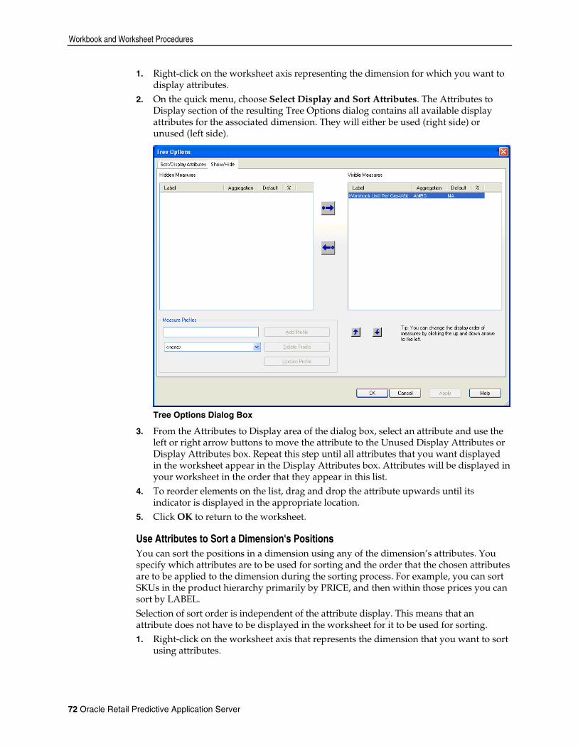
Workbook and Worksheet Procedures
72 Oracle Retail Predictive Application Server
1. Right-click on the worksheet axis representing the dimension for which you want to display attributes.
2. On the quick menu, choose Select Display and Sort Attributes. The Attributes to Display section of the resulting Tree Options dialog contains all available display attributes for the associated dimension. They will either be used (right side) or unused (left side).
Tree Options Dialog Box
3. From the Attributes to Display area of the dialog box, select an attribute and use the left or right arrow buttons to move the attribute to the Unused Display Attributes or Display Attributes box. Repeat this step until all attributes that you want displayed in the worksheet appear in the Display Attributes box. Attributes will be displayed in your worksheet in the order that they appear in this list.
4. To reorder elements on the list, drag and drop the attribute upwards until its indicator is displayed in the appropriate location.
5. Click OK to return to the worksheet.
Use Attributes to Sort a Dimension's Positions You can sort the positions in a dimension using any of the dimension’s attributes. You specify which attributes are to be used for sorting and the order that the chosen attributes are to be applied to the dimension during the sorting process. For example, you can sort SKUs in the product hierarchy primarily by PRICE, and then within those prices you can sort by LABEL. Selection of sort order is independent of the attribute display. This means that an attribute does not have to be displayed in the worksheet for it to be used for sorting. 1. Right-click on the worksheet axis that represents the dimension that you want to sort
using attributes.
Using Workbooks, Worksheets, and Wizards
Using Workbooks, Worksheets, and Wizards 73
2. On the quick menu, choose Select Display and Sort Attributes. The Attributes to Sort By area of the Tree Options dialog box contains all of the available sort attributes for the associated dimension. They will either be used (right side) or unused (left side).
3. From the Attributes to Sort By area of the dialog box, select an attribute and use the left or right arrow buttons to move the attribute to the Unused Sort Attributes or Sort Attributes box. Repeat this step until all attributes that you want displayed in the worksheet appear in the Sort Attributes box.
4. During the sorting process, attributes will be applied to the dimension’s positions in the order that they appear in the Sort Attributes box.
5. To reorder attributes in the Sort Attributes box, drag and drop the attribute upwards until its indicator is displayed in the appropriate location.
6. Click OK to return to the worksheet.
Sorting Positions in Multiple Windows The selections for sort attributes for a single dimension may differ from worksheet window to worksheet window. This feature is useful when different views (provided by different sorts) of the data are desired at the same time. You can use the New Window command on the Window menu to create a copy of the current worksheet. Each copy of the worksheet is represented by a different window and can contain data that is sorted using a different sort method.
Sort Measures Using the User Specified Sort Order Function When sorting and displaying measures, the “User-Specified Sort Order” can be used to dictate an exact order that measure positions should be displayed in the grid. The User Specified Sort Order allows you to rearrange measures so that they are displayed in an arbitrary order that you determine. This method allows you to select more specific sort orders that cannot be attained by ordering the sort attributes in the Sort Attributes box. You can still sort positions in the Measure hierarchy according to any of that hierarchy’s attributes. This way, the Measure hierarchy is no different from any other hierarchy represented by your data. For instance, you can specify that all measures should be sorted in the worksheet according to aggregation method. In this case, all measures with an aggregation method of ‘Period End Total’ would be grouped together and displayed before measures with an aggregation method of ‘Recalculated,’ which would appear before measures with a ‘Total’ aggregation method. The system sorts measure positions alphanumerically based on the values assigned to the sort attribute in question. It is more likely that you will want to specify a particular measure ordering scheme that cannot be attained by sorting the positions based on attributes. The User Specified Sort Order feature is designed to help you attain this specialized view. When the User Specified Sort Order feature is enabled, it overrides any attribute sorting scheme specified on the Select Display and Sort Attributes dialog. When selected, this feature orders measure positions in your worksheet that are based on their current order as presented in the Show/Hide dialog. To change the order of the measures in your worksheet display, change the order of measures on the list in the Show/Hide dialog. 1. Right-click within the Measure axis, and choose Select Display and Sort Attributes
from the quick menu.

Workbook and Worksheet Procedures
74 Oracle Retail Predictive Application Server
Select display and sort attributes Menu Option
2. Below the Attributes to Sort By area, select the Sort by user specified sort order option.
Note: When this option is selected, the Unused Sort Attributes box and Sort Attributes box become disabled. The User Specified Sort Order feature overrides any selections made in these boxes.
3. Click the Show/Hide Measures tab. 4. Select a measure in the Visible Measures box.

Using Workbooks, Worksheets, and Wizards
Using Workbooks, Worksheets, and Wizards 75
Example of Visible Measures Box in Show/Hide Tab
Note: This illustration only has one measure so the following step would not apply. Normally, multiple measures appear.
5. Click the up arrow or down arrow to move the selected measure up or down in the list display.
6. Repeat steps 4-5 for measures as required until the desired display order is attained. The order of the measures in the Visible Measures box will match the order of measures in your worksheet.
7. Click OK.
Return to an Attribute Sorting Scheme To disable the User Specified Sort Order; and again sort your measures using attributes, return to the Select Display and Sort Attributes dialog, and clear the Sort By User Specified Sort Order check box. The Unused Sort Attributes and Sort Attributes list boxes become enabled, which allows you to make sort attribute selections as desired.
Sort Measure Data in Multiple Windows The selections for sort attributes for a single dimension can differ from worksheet window to worksheet window. This feature is useful when different views (provided by different sorts) of the data are desired at the same time. You can use the New Window command on the Window menu to create a copy of the current worksheet. Each copy of the worksheet is represented by a different window, and can contain measure data that is sorted using a different sort method.
Sort a Dimension by Grid Data Values The sorting mechanism allows you to sort one dimension in a hierarchy according to the current data values in the grid. You do this by specifying a one-dimensional data space for a given dimension, and then by creating a user-named attribute based on that selected data. That attribute can then be used to sort and resort data in the corresponding dimension.

Workbook and Worksheet Procedures
76 Oracle Retail Predictive Application Server
Example Suppose that you want to sort all product classes in your product hierarchy in ascending order based on the total sales for each during the month of January. In this case, the dimension you want to sort is product class. To define the necessary one-dimensional data space, you must aggregate total sales for the product class dimension to the month level and select the January position. The one-dimensional data space is essentially a single row or column of data corresponding to the dimension you want to sort. Once you have selected the data that you want to sort, you must create a system-recognized sort attribute based on this data. You might choose to call this attribute "JanSales." Once an attribute is created, it can be used to perform the initial data sort, and can later be used for resorts of that same dimension if changes to the data occur.
Sort Hierarchies by Data Values in the Grid Use the following procedure to sort one dimension in a hierarchy according to a set of data values in the grid: 1. Select a one-dimensional data space of grid data (a single column or row of data) to
be sorted. 2. From the View menu, select Sort, or right-click over the axis for the dimension you
are sorting to produce a quick menu, and select Sort. 3. On the Create Sort Attribute dialog box, enter a label for the sort attribute.
Create Sort Attribute Dialog Box
4. Choose a name that will help you identify what this particular sort accomplishes (for example, JanSales for a group of products to be sorted according to their total January sales).
Note: If the dimension you are sorting is displayed in outline mode with other dimensions in that hierarchy, the Create Sort Attribute dialog will contain an additional field. This additional field allows you to specify the single dimension in which to apply the created sort attribute.
5. Click the appropriate radio button to specify the desired sort order (Ascending or Descending).
6. Click OK. The initial sort of the selected data occurs.
Re-Sort/Update a Dimension Using an Already Defined Sort Attribute If changes to sorted data occur, you may want to re-sort the dimension based on the new values. Follow this procedure to reapply a sort attribute to a selected dimension. 1. Right-click over the axis for the dimension to be resorted. A quick menu is displayed. 2. Select Resort. The data is re-sorted according to the current attribute sort order
specified for that dimension.
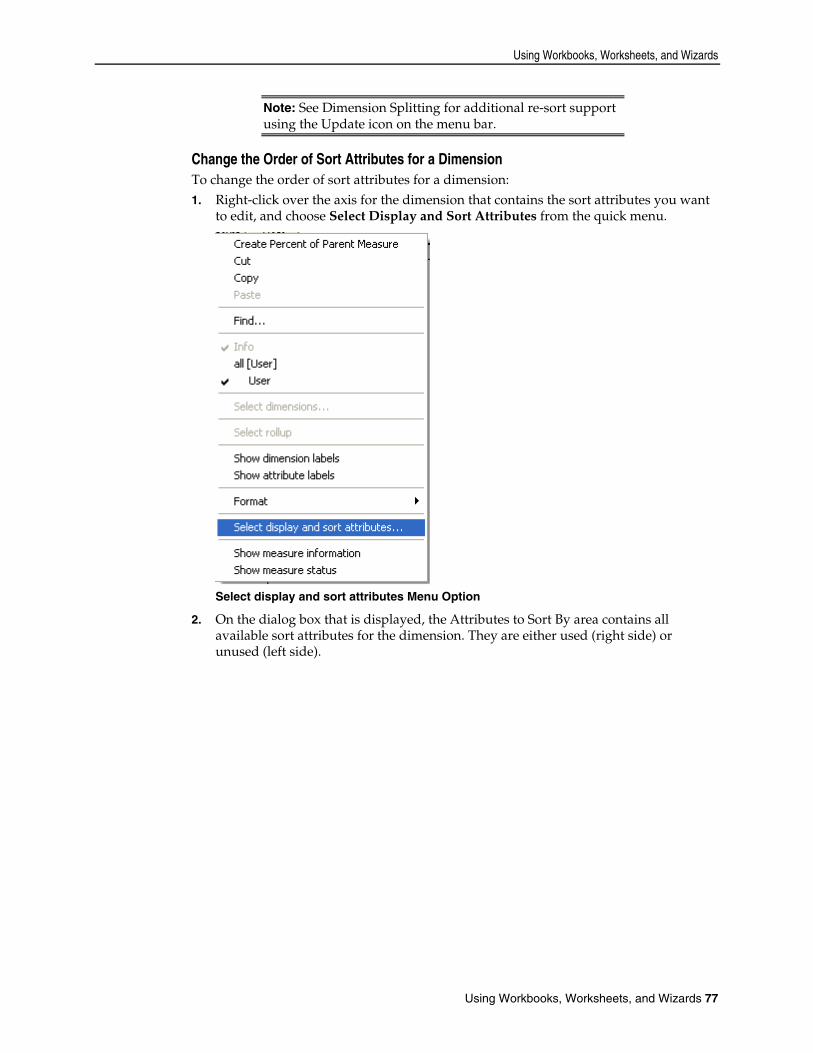
Using Workbooks, Worksheets, and Wizards
Using Workbooks, Worksheets, and Wizards 77
Note: See Dimension Splitting for additional re-sort support using the Update icon on the menu bar.
Change the Order of Sort Attributes for a Dimension To change the order of sort attributes for a dimension: 1. Right-click over the axis for the dimension that contains the sort attributes you want
to edit, and choose Select Display and Sort Attributes from the quick menu.
Select display and sort attributes Menu Option
2. On the dialog box that is displayed, the Attributes to Sort By area contains all available sort attributes for the dimension. They are either used (right side) or unused (left side).

Workbook and Worksheet Procedures
78 Oracle Retail Predictive Application Server
Example of Tree Options Dialog Box
3. If desired, click a sort attribute to highlight it, and use the left or right arrow buttons to move the attribute to the desired side of the screen.
4. To reorder the elements on the list, drag and drop the attribute upwards until its indicator is in the appropriate location.
5. Attributes in the Sort Attributes list box are reordered according to your actions. The order of attributes on this list specifies the major to minor sorting scheme that the system applies to the dimension each time the Sort or Resort command is invoked.
6. Click OK.
Dimension Splitting The RPAS Dimension Splitting features allow users to set-up, view, and manipulate data using dynamic, ad-hoc attribute hierarchies. This is achieved by building dynamic hierarchies where attribute values become positions within a dimension. Once a dynamic hierarchy is created, all grid-type features such as editing, locking, protection processing, etc., are fully functional (see “Adding a New Dynamic Attribute” for more information on building and maintaining dynamic attribute hierarchies). Once a workbook is saved with a dimension split, the split is retained for the lifetime of the workbook. You also have the ability to apply saved splits in new workbooks, eliminating the need to redefine the split. The following is a summary of use cases that Dimension Splitting supports: At any step in the workflow, the user splits a single dimension in a single hierarchy
using the Dimension Splitting Dialog. Only one dimension can be split in any hierarchy, though dimensions in many hierarchies may be split at a given point in time. This is achieved through multiple invocations of the Dimension Splitting Dialog, once for each hierarchy whose dimension is being split.

Using Workbooks, Worksheets, and Wizards
Using Workbooks, Worksheets, and Wizards 79
The user is able to specify a split definition by picking one or more (a maximum of four) attributes from a list of all splitting attributes for a given dimension. Once such a split is defined, but not necessarily saved or catalogued, the user is able to exercise the split computation and view it.
The user is able to save a split definition to the domain catalogue without viewing it.
The user is able to view an existing (catalogued in the domain) split definition. The user is able to modify an existing (catalogued in the domain) split definition. The user is able to modify an existing split definition and save it as a new split
definition in the domain. The user is able to delete an existing split definition. The user is able to view an existing split. The user is able to save a split definition to the domain catalogue after viewing the
split.
Split a Dimension Based on an Attribute
Navigate Right-click over the hierarchy tile or positions in which the split will apply, select the Split Dimension menu. From this menu, you can view the Dimension Splitting dialog box.
Dimension Splitting Dialog Box

Workbook and Worksheet Procedures
80 Oracle Retail Predictive Application Server
1. The Select Dimension box defaults to the dimension in which the user initiated the Dimension Splitting dialog. The Available Splits and Split Definitions boxes will display values if attributes have been defined that match the dimension to be split. If no values are populated in the Available Splits or Split Definitions boxes, there are no attributes defined that match the dimension selected to split. To define an applicable attribute, select Open Attribute Definitions (see “Adding a New Dynamic Attribute” for more information on building and maintaining dynamic attribute hierarchies).
2. From the Select Dimension box, you may also change the dimension to split. If the dimension is modified, click Select to populate the Available Splits and the Split Definition boxes. If there are no values in the Available Splits and Split Definition boxes, return to the previous step.
3. The Available Splits box displays split definitions that have been previously saved by the user in this or other workbooks. You may apply a previously saved split definition to the current worksheet. A single saved split can be applied from this dialog box using the arrow keys to move the saved split(s) to the Attributes to be used in split box. The Attributes to be used in split box will update to reflect the attribute associated with the saved split selected by the user, rather than the label of the saved split.
4. The Split Definition box displays the user’s attribute definitions that may be applied to the dimension to be split. Single or multiple attributes can be applied from this window using the arrow keys to move the attribute(s) to the Attributes to be used in split box. The maximum number of attributes that a dimension can be split upon is 4.
5. Select OK to view the data in the worksheet along the split dimension. 6. Once the split dimension can be viewed in the worksheet, you may split another
dimension along different hierarchy in the same view. Right-click over a different hierarchy tile or positions in which the split will apply, select the Split Dimension menu. See Step 1 to continue.
Note: Dimensions along the calendar hierarchy cannot be split.
Save a Split Dimension Saved (or cataloged) split definitions allow the user to apply a previously defined dimension split to a new workbook. A split is only saved along a single dimension although the user may be viewing data using a multi-dimension split (two attributes, each along different hierarchies). 1. Once a dimension split has been applied to the worksheet, you can save the split by
right-clicking over the hierarchy tile or positions in which the split applies and selecting the Save Current Split menu.
2. Enter the label for the saved split definition and select OK. 3. You can unsplit the dimension and re-apply the saved dimension split or apply it
once in a new workbook.

Using Workbooks, Worksheets, and Wizards
Using Workbooks, Worksheets, and Wizards 81
Note: It is not necessary to save a split definition to view it. The user can simply create an arbitrary split definition in the Split Definition box and view it without saving. If a saved (catalogued) split definition is changed but not saved before the user moves to a different split definition or exits the dialog, the user will be prompted to save or discard the changes to the catalogued split definition. If a saved (catalogued) split definition becomes invalid (but not unusable) due to unavailability (deletion) of one or more of its defining attributes, or unusable due to unavailability of all its defining attributes, the user will see a message indicating the split is no longer valid.
Unsplit a Dimension Once a dimension split has been applied to the worksheet, the user can unsplit the dimension by right-clicking over the hierarchy tile or positions in which the split applies and select the Unsplit Dimension menu. The user may repeat this step to unsplit additional dimensions in the worksheet.
Delete a Saved Dimension Split 1. To delete a saved dimension split, the user must first unsplit the dimension in which
the saved dimension split applies. 2. Right-click over the hierarchy tile or positions in which the saved dimension split
applies, select the Split Dimension menu. 3. The Available Splits box displays the split definitions that have been previously
saved by the user in this or other workbooks. Highlight the saved dimension split to be deleted and click Delete. Repeat for additional saved splits.
Note: This action permanently removes the saved split definition from the system, preventing the split from being re-applied in the same workbook or new workbooks that are built. No commit from the workbook is required for the deletion to be made permanent.
Dynamic Position Maintenance (Dynamic Add) Dynamic Position Maintenance (DPM) enables users to dynamically add or remove positions to a non-calendar dimension while working in a workbook. These user-defined or ‘informal’ positions are updated in both the domain and workbook hierarchies. Positions added by the user are referred to as ‘informal’ positions versus positions added during the hierarchy load process are referred to as ‘formal’ positions. If/when the informal position is to be made formal, the position’s name (label is not necessary for the update to occur) must first be updated to reflect the correct position name that will be loaded during the hierarchy load process. Prior to the hierarchy load, an administrative utility is run against the environment to change the status of a position from informal to formal (see the RPAS Administration Guide for more information on the ‘updateDpmPositionStatus’ utility). This process will enable the loading and purging of that position through the hierarchy load process and will disable further DPM activities on the position.
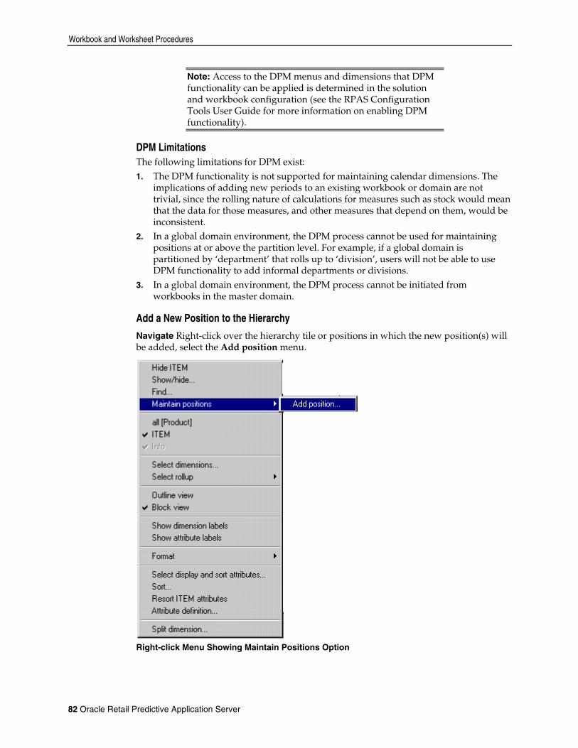
Workbook and Worksheet Procedures
82 Oracle Retail Predictive Application Server
Note: Access to the DPM menus and dimensions that DPM functionality can be applied is determined in the solution and workbook configuration (see the RPAS Configuration Tools User Guide for more information on enabling DPM functionality).
DPM Limitations The following limitations for DPM exist: 1. The DPM functionality is not supported for maintaining calendar dimensions. The
implications of adding new periods to an existing workbook or domain are not trivial, since the rolling nature of calculations for measures such as stock would mean that the data for those measures, and other measures that depend on them, would be inconsistent.
2. In a global domain environment, the DPM process cannot be used for maintaining positions at or above the partition level. For example, if a global domain is partitioned by ‘department’ that rolls up to ‘division’, users will not be able to use DPM functionality to add informal departments or divisions.
3. In a global domain environment, the DPM process cannot be initiated from workbooks in the master domain.
Add a New Position to the Hierarchy
Navigate Right-click over the hierarchy tile or positions in which the new position(s) will be added, select the Add position menu.
Right-click Menu Showing Maintain Positions Option

Using Workbooks, Worksheets, and Wizards
Using Workbooks, Worksheets, and Wizards 83
From this menu, you can view the Dynamic Position Maintenance dialog box. The structure for the selected hierarchy, with the lowest child dimension displayed at the top, appears. A writable (non-gray) field next to a dimension indicates that an informal
position may be added to the dimension. The folder icon next to a dimension indicates that the user may select an existing position in the hierarchy to associate as a parent or child of a newly added position. All dimensions along the main branch of the hierarchy and the alternate branches must be populated with a position value before the user is able to save and view the new informal position(s) in the workbook. For the dimensions that are not writable and do not include a folder icon, the position will be automatically populated based on the immediate child position selected.
Dynamic Position Maintenance Dialog Box
1. Select the dimension that will have a new position added (from the writable, non-gray fields).
2. Enter the new position label. The position label is the description of the position that the user sees in the RPAS Client. As you begin to type in the value for the position label, the Position Description dialog box appears.
3. Enter the new position name. The position name is the RPAS internal identifier associated with the position label. Select OK to add the position.
Example of Position Description Dialog Box

Workbook and Worksheet Procedures
84 Oracle Retail Predictive Application Server
Note: The position name may contain alpha-numeric characters including “_” underscores. However the position name must begin with an alpha character and cannot contain white spaces.
4. After adding a new position, add new positions for other writable dimensions, or use
the folder icon to view the available formal or informal positions in the other selected dimensions that may be defined as a parent or child of the new position(s).
Example of Dynamic Positions Maintenance Dialog Box
5. Once the hierarchy is fully populated with position values, click OK or Apply to add the new informal position(s) to the hierarchy. Select OK to exit out of the Dynamic Position Maintenance window. Select Apply to remain in the Dynamic Position Maintenance dialog box, if
additional modifications to the positions are required. Select Cancel to close the Dynamic Position Maintenance window, ignoring the
user’s position changes. 6. You can now view the newly added position(s) in the workbook. All informal
positions in the workbook appear in blue.

Using Workbooks, Worksheets, and Wizards
Using Workbooks, Worksheets, and Wizards 85
Example of New Informal Positions in Workbook
Modify an Informal Position Once informal positions are added to the hierarchy, the DPM process allows you to: Change the parent of an informal position to another formal or informal parent. Update the position name and position label.
Navigate Right-click over the hierarchy tile or positions in which informal position(s) will be modified, select the Modify position menu. The Select Product dialog box appears
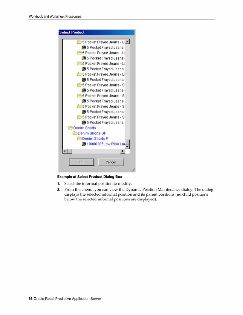
Workbook and Worksheet Procedures
86 Oracle Retail Predictive Application Server
Example of Select Product Dialog Box
1. Select the informal position to modify. 2. From this menu, you can view the Dynamic Position Maintenance dialog. The dialog
displays the selected informal position and its parent positions (no child positions below the selected informal positions are displayed).
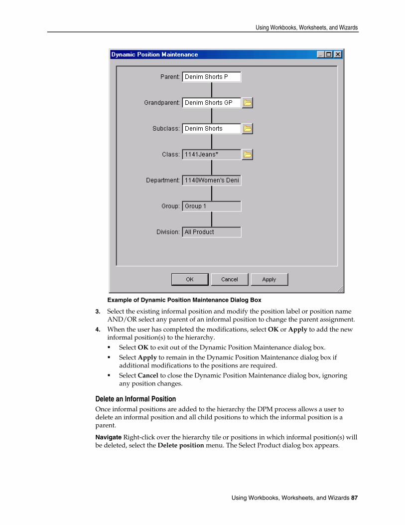
Using Workbooks, Worksheets, and Wizards
Using Workbooks, Worksheets, and Wizards 87
Example of Dynamic Position Maintenance Dialog Box
3. Select the existing informal position and modify the position label or position name AND/OR select any parent of an informal position to change the parent assignment.
4. When the user has completed the modifications, select OK or Apply to add the new informal position(s) to the hierarchy. Select OK to exit out of the Dynamic Position Maintenance dialog box. Select Apply to remain in the Dynamic Position Maintenance dialog box if
additional modifications to the positions are required. Select Cancel to close the Dynamic Position Maintenance dialog box, ignoring
any position changes.
Delete an Informal Position Once informal positions are added to the hierarchy the DPM process allows a user to delete an informal position and all child positions to which the informal position is a parent.
Navigate Right-click over the hierarchy tile or positions in which informal position(s) will be deleted, select the Delete position menu. The Select Product dialog box appears.
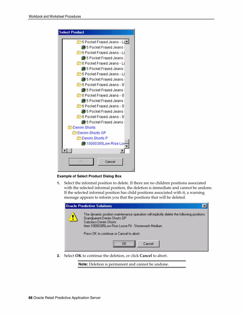
Workbook and Worksheet Procedures
88 Oracle Retail Predictive Application Server
Example of Select Product Dialog Box
1. Select the informal position to delete. If there are no children positions associated with the selected informal position, the deletion is immediate and cannot be undone. If the selected informal position has child positions associated with it, a warning message appears to inform you that the positions that will be deleted.
2. Select OK to continue the deletion, or click Cancel to abort.
Note: Deletion is permanent and cannot be undone.

Using Workbooks, Worksheets, and Wizards
Using Workbooks, Worksheets, and Wizards 89
Lock and Unlock Cells and Measures
Cell Locking and Unlocking The cell locking feature allows you to "lock" one or more editable cells in the grid. When a grid cell is locked, calculations performed as a result of data manipulations do not affect the locked data values. This functionality allows you examine various "what-if" scenarios to determine the best course of action for planning or forecasting. The "locked" status of a cell is indicated by the presence of a picture of a lock in the cell’s left portion. Once an eligible cell is locked, the system determines whether the remaining grid cells are eligible or ineligible to be locked. If a cell becomes ineligible to be locked, the right-click menu associated with that cell will not contain the Lock option. Furthermore, any read/write cells that become ineligible for locking are made read-only. You may choose to lock a data cell at any time to protect that cell from forced recalculations due to data manipulations elsewhere in the worksheet. For example, you may want to see the effect of a change to Sales Value on Inventory levels without forcing a change to Receipts. Another example would be to change Sales Value at an aggregate level (such as Month) and spread the result to only three of the four weeks that comprise that month. In this case, you could effectively hold the second week’s Sales Value constant while spreading the aggregate-level increase among the remaining three weeks.
Note: All cells that belong to a measure with aggregation type "AMBG" or "AMBGP" and represent values at an intersection higher than the base intersection cannot be locked. The "Lock Cell" menu item obtained on the right click menu will not be available for such cells.
Examples of Cell Locking The following topic describes two typical examples of cell locking usage. Example 1: Using Cell Locking to Affect Spreading/Aggregation Suppose you want to change a sales value at an aggregate level (for instance, Month) and spread this result to three out of four underlying cells while holding the fourth constituent cell value constant. Without the use of the cell locking feature, a change that is made to the Month-level cell will force a recalculation of all underlying Week-level cells that roll up into that month. The cell locking feature allows you to hold the value of one week constant while spreading the effects of the aggregate-level change to the remaining three weeks. In the following example, suppose you want to change the January sales value for clock radios from 2200 to 3900 while holding the week 2 sales value of 500 constant. Right-click in the cell that contains the sales value for clock radios in the second week of January. Select Lock Cell from the resulting pop-up menu.
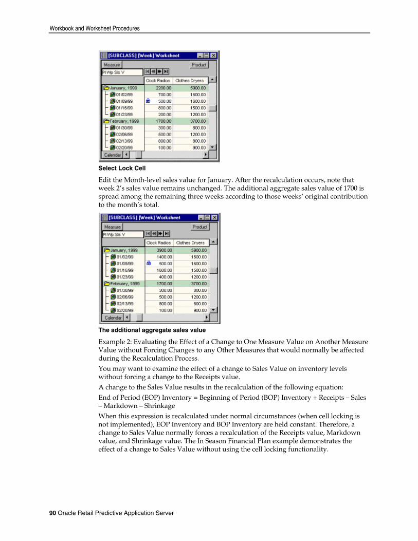
Workbook and Worksheet Procedures
90 Oracle Retail Predictive Application Server
Select Lock Cell
Edit the Month-level sales value for January. After the recalculation occurs, note that week 2’s sales value remains unchanged. The additional aggregate sales value of 1700 is spread among the remaining three weeks according to those weeks’ original contribution to the month’s total.
The additional aggregate sales value
Example 2: Evaluating the Effect of a Change to One Measure Value on Another Measure Value without Forcing Changes to any Other Measures that would normally be affected during the Recalculation Process. You may want to examine the effect of a change to Sales Value on inventory levels without forcing a change to the Receipts value. A change to the Sales Value results in the recalculation of the following equation: End of Period (EOP) Inventory = Beginning of Period (BOP) Inventory + Receipts – Sales – Markdown – Shrinkage When this expression is recalculated under normal circumstances (when cell locking is not implemented), EOP Inventory and BOP Inventory are held constant. Therefore, a change to Sales Value normally forces a recalculation of the Receipts value, Markdown value, and Shrinkage value. The In Season Financial Plan example demonstrates the effect of a change to Sales Value without using the cell locking functionality.
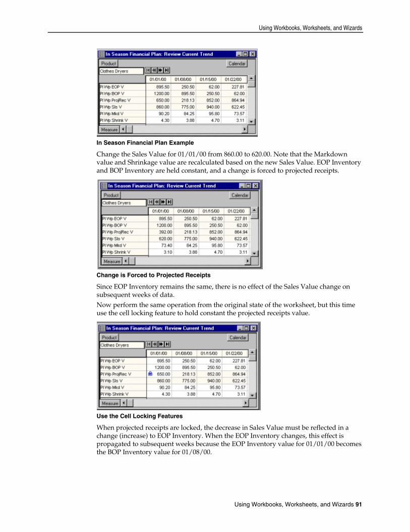
Using Workbooks, Worksheets, and Wizards
Using Workbooks, Worksheets, and Wizards 91
In Season Financial Plan Example
Change the Sales Value for 01/01/00 from 860.00 to 620.00. Note that the Markdown value and Shrinkage value are recalculated based on the new Sales Value. EOP Inventory and BOP Inventory are held constant, and a change is forced to projected receipts.
Change is Forced to Projected Receipts
Since EOP Inventory remains the same, there is no effect of the Sales Value change on subsequent weeks of data. Now perform the same operation from the original state of the worksheet, but this time use the cell locking feature to hold constant the projected receipts value.
Use the Cell Locking Features
When projected receipts are locked, the decrease in Sales Value must be reflected in a change (increase) to EOP Inventory. When the EOP Inventory changes, this effect is propagated to subsequent weeks because the EOP Inventory value for 01/01/00 becomes the BOP Inventory value for 01/08/00.

Workbook and Worksheet Procedures
92 Oracle Retail Predictive Application Server
The Decrease in Sales Value
Locking a Grid Cell To lock a grid cell: 1. Right-click in the cell you want to lock. 2. Select Lock Cell from the pop-up menu. 3. A picture of a lock displays in the cell to indicate that the cell’s status is locked. When
recalculations of grid values are performed, the locked cell’s value will be held constant, which means that data manipulations that would normally force a change to the locked cell’s value will now result in no change to the locked data.
Note: If the Lock option is not displayed on a particular cell’s right-click menu, that cell is ineligible to be locked. This condition occurs as a result of the placement of other locks elsewhere in the worksheet. Cells that exist at a different hierarchical level than a locked cell may be ineligible for locking if they exist along a different path of aggregation.
Unlock a Single Grid Cell To unlock a single grid cell: 1. Right-click in the cell you want to unlock. 2. Select Unlock Cell from the pop-up menu.
Unlock all Currently Locked Grid Cells To unlock all currently locked grid cells: 1. Right-click any grid cell. 2. Select Unlock All Cells from the pop-up menu.
Measure Locking The Measure Locking feature allows you to simultaneously lock all of the cells that are associated with a given measure in a worksheet. As with individual cell locking, the locked status of each cell in the measure is indicated by the lock picture in each cell’s left portion. A locked measure is also indicated by the appearance of the lock image in the axis header for that measure.
Lock a Worksheet Measure To lock a worksheet measure: 1. Right-click over the axis label for the measure you want to lock. 2. On the quick menu, select the Lock Measure option.
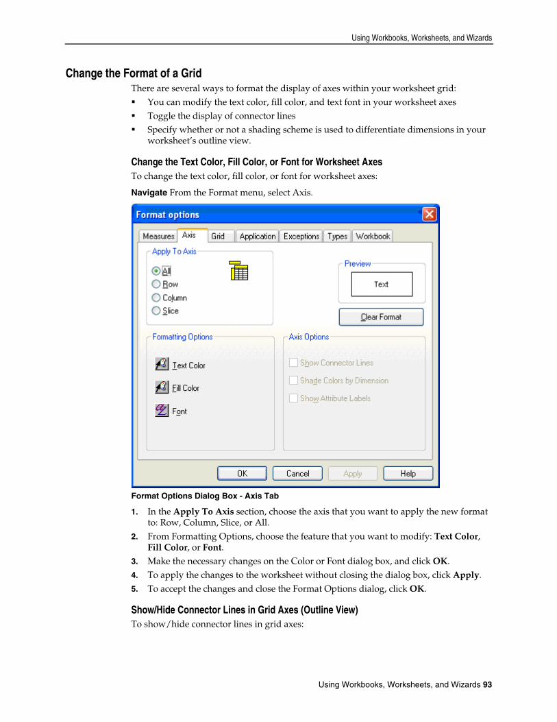
Using Workbooks, Worksheets, and Wizards
Using Workbooks, Worksheets, and Wizards 93
Change the Format of a Grid There are several ways to format the display of axes within your worksheet grid: You can modify the text color, fill color, and text font in your worksheet axes Toggle the display of connector lines Specify whether or not a shading scheme is used to differentiate dimensions in your
worksheet’s outline view.
Change the Text Color, Fill Color, or Font for Worksheet Axes To change the text color, fill color, or font for worksheet axes:
Navigate From the Format menu, select Axis.
Format Options Dialog Box - Axis Tab
1. In the Apply To Axis section, choose the axis that you want to apply the new format to: Row, Column, Slice, or All.
2. From Formatting Options, choose the feature that you want to modify: Text Color, Fill Color, or Font.
3. Make the necessary changes on the Color or Font dialog box, and click OK. 4. To apply the changes to the worksheet without closing the dialog box, click Apply. 5. To accept the changes and close the Format Options dialog, click OK.
Show/Hide Connector Lines in Grid Axes (Outline View) To show/hide connector lines in grid axes:

Workbook and Worksheet Procedures
94 Oracle Retail Predictive Application Server
Note: Connector lines are only displayed when an axis is viewed in outline mode.
Navigate From the Format menu, select Axis. 1. In the Apply To Axis section, choose the axis that you want to apply the new format
to. The Show Connector Lines option can only be applied to one axis at a time (Row, Column, or Slice).
2. From Axis Options, select the Show Connector Lines check box to display lines. Clear this check box to remove the lines.
3. To apply the change to the worksheet without closing the dialog box, click Apply. 4. To accept the change and close the Format Options dialog, click OK.
Specify a Shading Scheme to Differentiate Dimensions (Outline View)
Note: This option only has an effect when you are viewing an axis in outline mode. A shading scheme to differentiate dimensions will override any selection made regarding the specified color for read/write cells.
Navigate From the Format menu, select Axis.
Format Options Dialog Box - Axis Tab
1. In the Apply To Axis section, choose the axis to which to apply the shading scheme. The Shade Colors By Dimension option can only be applied to one axis at a time (Row, Column, or Slice).

Using Workbooks, Worksheets, and Wizards
Using Workbooks, Worksheets, and Wizards 95
2. From Axis Options, select the Shade Colors By Dimension check box to use the shading scheme. Regardless of dimension, clear this check box to display all cells of a given measure in the same manner.
3. To apply the change to the worksheet without closing the dialog box, click Apply. 4. To accept the change and close the Format Options dialog, click OK.
Specify the Appearance of Attribute Labels in the Axis Display To specify the appearance of attribute labels in the axis display:
Note: This option turns on or off the display of attribute labels, and it is only applied to the Row Axis and the Column Axis. To turn on the display of position attribute values, right-click over the desired axis, and choose Select Display and Sort Attributes from the menu.
Navigate From the Format menu, select Axis.
Format Options Dialog Box - Axis Tab
1. In the Apply to Axis section, choose either the row axis or the column axis. 2. From the Axis Options, check the Show Attribute Labels option to display labels. 3. Clear the option to turn off the display. 4. To apply the change to the worksheet without closing the dialog box, click Apply, or
to accept the change and close the Format Options dialog, click OK.

Workbook and Worksheet Procedures
96 Oracle Retail Predictive Application Server
Format Grid Components
Change the Background Color of the Grid Display Follow this procedure to modify the color of the grid background. The grid background is the portion of the window behind the data grid, hierarchy tiles, and axes.
Navigate From the Format menu, select Application. 1. Under Color Options, click Grid Background Color.
Color Options
2. Make a color selection for the grid background. 3. Click OK. 4. To apply the change to the worksheet without closing the dialog box, click Apply, or
to accept the change and close the Format Options dialog, click OK.
Format the Display of Grid Lines Follow these procedures to specify the appearance of grid lines in your worksheet. You can turn on or off the display of horizontal and vertical grid lines. If grid lines are displayed, you can specify their color.
Change the Color of Grid Lines in your Worksheet To change the color of grid lines in your worksheet:
Navigate From the Format menu, select Grid.
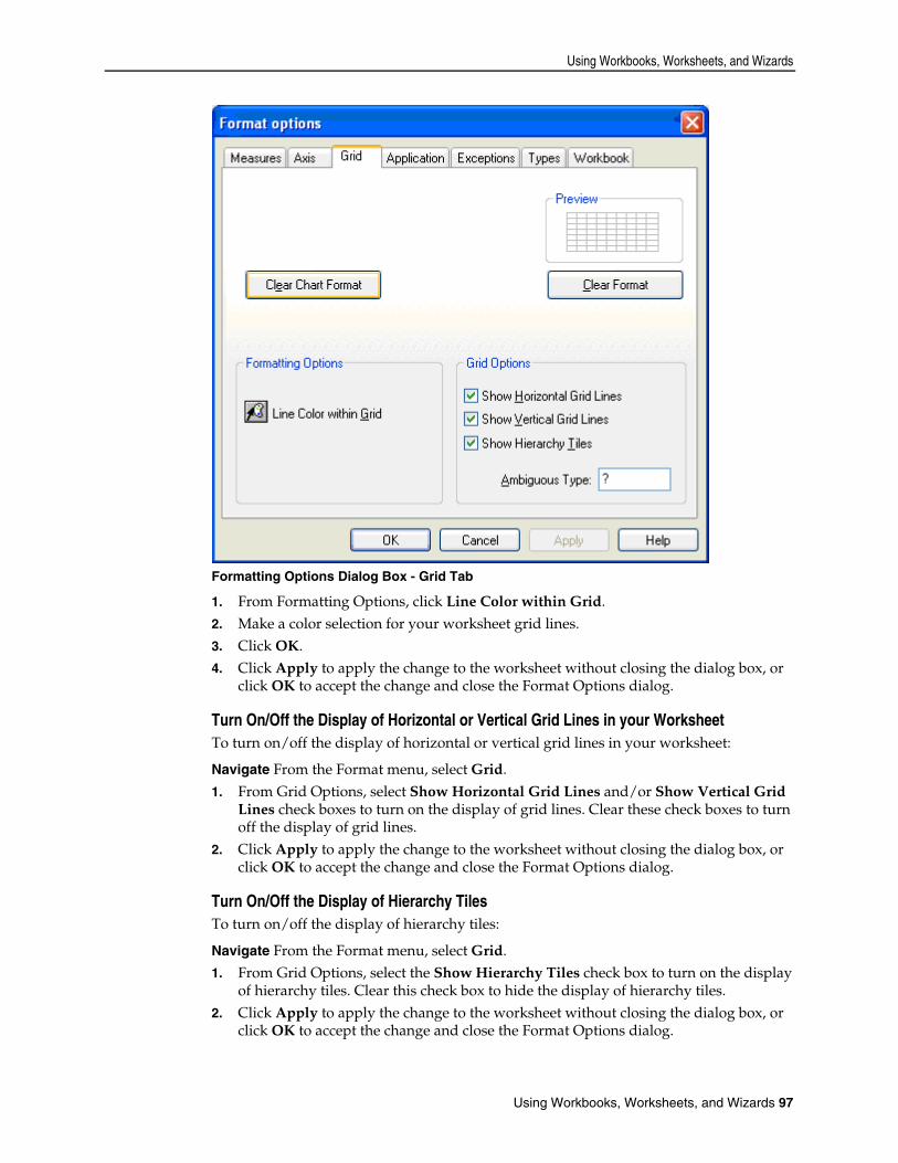
Using Workbooks, Worksheets, and Wizards
Using Workbooks, Worksheets, and Wizards 97
Formatting Options Dialog Box - Grid Tab
1. From Formatting Options, click Line Color within Grid. 2. Make a color selection for your worksheet grid lines. 3. Click OK. 4. Click Apply to apply the change to the worksheet without closing the dialog box, or
click OK to accept the change and close the Format Options dialog.
Turn On/Off the Display of Horizontal or Vertical Grid Lines in your Worksheet To turn on/off the display of horizontal or vertical grid lines in your worksheet:
Navigate From the Format menu, select Grid. 1. From Grid Options, select Show Horizontal Grid Lines and/or Show Vertical Grid
Lines check boxes to turn on the display of grid lines. Clear these check boxes to turn off the display of grid lines.
2. Click Apply to apply the change to the worksheet without closing the dialog box, or click OK to accept the change and close the Format Options dialog.
Turn On/Off the Display of Hierarchy Tiles To turn on/off the display of hierarchy tiles:
Navigate From the Format menu, select Grid. 1. From Grid Options, select the Show Hierarchy Tiles check box to turn on the display
of hierarchy tiles. Clear this check box to hide the display of hierarchy tiles. 2. Click Apply to apply the change to the worksheet without closing the dialog box, or
click OK to accept the change and close the Format Options dialog.

Workbook and Worksheet Procedures
98 Oracle Retail Predictive Application Server
Specify a Value to Appear in Ambiguous Type Cells Follow this procedure to specify the string to be displayed in an aggregate-level cell when it is not clear how the system should aggregate certain data values. This string indicates the presence of lower level data that cannot be displayed at a particular level of aggregation. For example, pick list-type data at the SKU level would aggregate ambiguously if different SKUs in the same Style contained different pick list values. Here, you can specify what the system should display in a Style-level cell.
Navigate From the Format menu, select Grid. 1. From Grid Options, enter a string in the Ambiguous Type (for example, Ambig)
field that should appear in all worksheet cells containing data that aggregates ambiguously.
2. To apply the change to the worksheet without closing the dialog box, click Apply, or to accept the change and close the Format Options dialog, click OK.
Change the Format of a Measure You can modify the text color, fill color, and text font of a measure’s cells and label. You can also specify the alignment, border style, and border color for the grid cells that are associated with a measure.
Format the Display of Text and Borders for Measure Cells and Labels To format the display of text and borders for measure cells and labels:
Navigate From the Format menu, select Measure.
Format Options Dialog Box - Measures Tab

Using Workbooks, Worksheets, and Wizards
Using Workbooks, Worksheets, and Wizards 99
1. In the Measure box (lower right of Measures tab), select all measures that contain the labels or cells that you want to reformat.
2. Select an Apply To option (Cells, Labels, or Both). 3. Select a Formatting Option (Text Color, Fill Color, Font, Alignment, Border Style,
or Border Color). 4. Make the necessary formatting changes in the dialog box you selected, and click OK. 5. Click Apply to apply the changes to the worksheet without closing the dialog box, or
click OK to accept the changes and close the Format Options dialog.
Set Application-Wide Formatting Options You can set application-wide formatting options for all workbooks viewed in the Oracle Retail Predictive Solutions. These formatting options include: The grid display background color. The color for both read-only and read/write worksheet cells. The appearance of toolbar button text. The appearance of the flow control tabs.
Enable/Disable the Display of the Toolbar Button Text Use this procedure to toggle the display of toolbar button names. When button text is turned on, the toolbar buttons appear large and include the button name/function. When button text is turned off, the buttons appear small and contain no text. 1. From the Format menu, select Application. 2. From Application Options, select Show Button Text. 3. Click Apply to apply the change to the worksheet without closing the dialog box, or
click OK to accept the change and close the Format Options dialog.
Set the Display Color for Read-Only and Read/Write Cells To set the display color for read-only and read/write cells:
Navigate From the Format menu, select Application. 1. From Color Options, click either Read Only Color or Read/Write Color to produce a
color palette for the selected cell type. 2. Make a color selection from the color palette, and click OK. 3. To apply the change to the worksheet without closing the dialog box, click Apply, or
to accept the change and close the Format Options dialog, click OK.
Note: The Read/Write Color selection will be overridden if the Shade Colors By Dimension option on the Format – Axis tab is selected. Dimension shading (if toggled on) overrides any read/write color selection, but it does not override the read only color selection. If your read/write color selection does not appear to be recognized by the system, try toggling off the Shade Colors By Dimension option on the Format – Axis tab.
Enable/Disable the Display of the Flow Control Tabs
Navigate From the Format menu, select Application. 1. Under Application Options, check the Show Tab Control option to turn on the tab
control display. Clear this option to turn off the display.
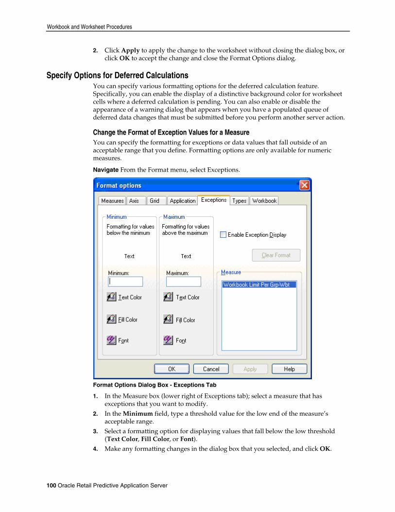
Workbook and Worksheet Procedures
100 Oracle Retail Predictive Application Server
2. Click Apply to apply the change to the worksheet without closing the dialog box, or click OK to accept the change and close the Format Options dialog.
Specify Options for Deferred Calculations You can specify various formatting options for the deferred calculation feature. Specifically, you can enable the display of a distinctive background color for worksheet cells where a deferred calculation is pending. You can also enable or disable the appearance of a warning dialog that appears when you have a populated queue of deferred data changes that must be submitted before you perform another server action.
Change the Format of Exception Values for a Measure You can specify the formatting for exceptions or data values that fall outside of an acceptable range that you define. Formatting options are only available for numeric measures.
Navigate From the Format menu, select Exceptions.
Format Options Dialog Box - Exceptions Tab
1. In the Measure box (lower right of Exceptions tab); select a measure that has exceptions that you want to modify.
2. In the Minimum field, type a threshold value for the low end of the measure’s acceptable range.
3. Select a formatting option for displaying values that fall below the low threshold (Text Color, Fill Color, or Font).
4. Make any formatting changes in the dialog box that you selected, and click OK.

Using Workbooks, Worksheets, and Wizards
Using Workbooks, Worksheets, and Wizards 101
5. In the Maximum field, type a threshold value for the high end of the measure’s acceptable range.
6. Select a formatting option for displaying values that exceed the high threshold (Text Color, Fill Color, or Font).
7. Make any formatting changes in the dialog box that you selected, and click OK. 8. Select Enable Exception Display to turn on the display of the exception formats you
selected. If this options is not selected, the exceptions will not be formatted in the grid, but the system will save your exception formatting selections, which can be enabled as needed.
9. To apply the changes to the worksheet without closing the dialog box, click Apply, or to accept the changes and close the Format Options dialog, click OK.
Enable/Disable the Display of a Deferred Calculation Warning Prompt Use this procedure to turn on or off the deferred calculation warning prompt. This message displays when you have a populated queue of data changes that must be submitted or canceled before you perform another server action. The system must deal with a populated queue before the server can be called for another reason, such as maximizing a currently minimized worksheet. When the warning message is turned on, a dialog will display before the data changes are sent to the server. This allows you to cancel the action if desired.
Navigate From the Format menu, select Application. The Application tab in the Format Options dialog box appears.
Format Options Dialog Box - Application Tab

Workbook and Worksheet Procedures
102 Oracle Retail Predictive Application Server
1. From Application Options, select Prompt for Deferred Calculations to enable the display of the warning prompt. If this option is left unchecked, queued data changes will be automatically sent to the server when you choose to perform another server-intensive action.
2. To apply the change to the worksheet without closing the dialog box, click Apply, or to accept the change and close the Format Options dialog, click OK.
Enable/Disable the Display of the Flow Control Tab
Navigate From the Format menu, select Application.
Format Options Dialog Box - Application Tab
1. Under the Application Options, select the Show Tab Control option to turn on the tab control display. Clear this option to turn off the display.
2. Click Apply to apply the change to the worksheet without closing the dialog box, or click OK to accept the change and close the Format Options dialog.
Enable/Disable Synchronized Page Scrolling
Navigate From the Format menu, select Workbook.

Using Workbooks, Worksheets, and Wizards
Using Workbooks, Worksheets, and Wizards 103
Format Options – Workbook Tab
Select Enable Synchronized Page Scrolling to enable the synchronized scrolling feature. Clear this option to disable the feature and support independent slice scrolling among the windows.
Enable/Disable the Display of the Selected Deferred Calculation Color To enable/disable the display of the selected deferred calculation color:
Navigate From the Format menu, select Application.
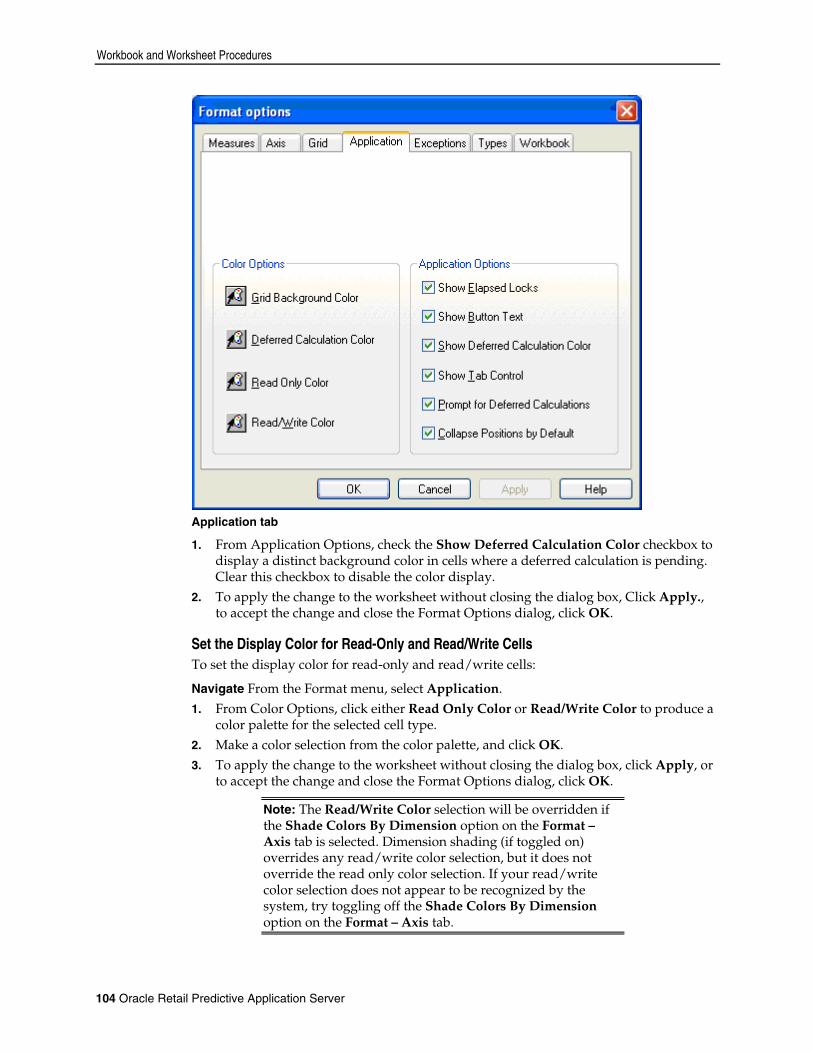
Workbook and Worksheet Procedures
104 Oracle Retail Predictive Application Server
Application tab
1. From Application Options, check the Show Deferred Calculation Color checkbox to display a distinct background color in cells where a deferred calculation is pending. Clear this checkbox to disable the color display.
2. To apply the change to the worksheet without closing the dialog box, Click Apply., to accept the change and close the Format Options dialog, click OK.
Set the Display Color for Read-Only and Read/Write Cells To set the display color for read-only and read/write cells:
Navigate From the Format menu, select Application. 1. From Color Options, click either Read Only Color or Read/Write Color to produce a
color palette for the selected cell type. 2. Make a color selection from the color palette, and click OK. 3. To apply the change to the worksheet without closing the dialog box, click Apply, or
to accept the change and close the Format Options dialog, click OK.
Note: The Read/Write Color selection will be overridden if the Shade Colors By Dimension option on the Format – Axis tab is selected. Dimension shading (if toggled on) overrides any read/write color selection, but it does not override the read only color selection. If your read/write color selection does not appear to be recognized by the system, try toggling off the Shade Colors By Dimension option on the Format – Axis tab.
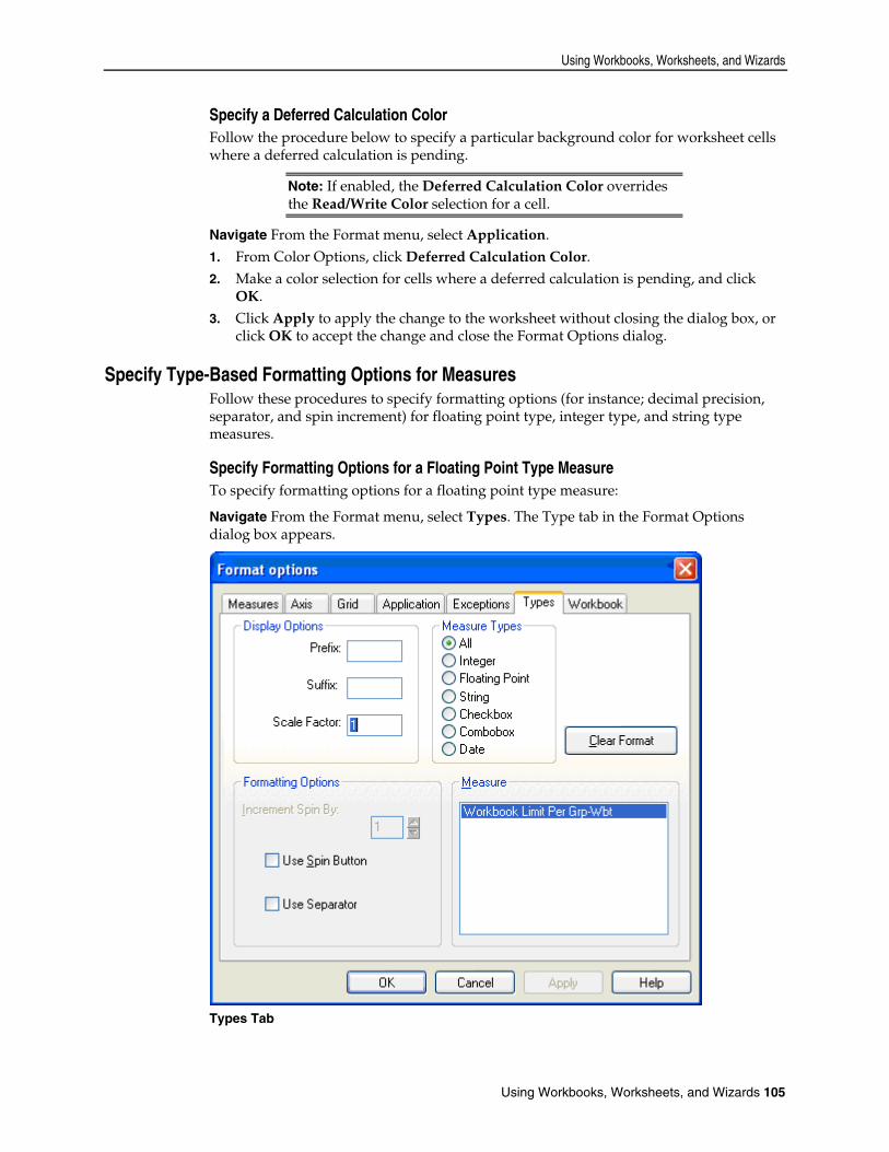
Using Workbooks, Worksheets, and Wizards
Using Workbooks, Worksheets, and Wizards 105
Specify a Deferred Calculation Color Follow the procedure below to specify a particular background color for worksheet cells where a deferred calculation is pending.
Note: If enabled, the Deferred Calculation Color overrides the Read/Write Color selection for a cell.
Navigate From the Format menu, select Application. 1. From Color Options, click Deferred Calculation Color. 2. Make a color selection for cells where a deferred calculation is pending, and click
OK. 3. Click Apply to apply the change to the worksheet without closing the dialog box, or
click OK to accept the change and close the Format Options dialog.
Specify Type-Based Formatting Options for Measures Follow these procedures to specify formatting options (for instance; decimal precision, separator, and spin increment) for floating point type, integer type, and string type measures.
Specify Formatting Options for a Floating Point Type Measure To specify formatting options for a floating point type measure:
Navigate From the Format menu, select Types. The Type tab in the Format Options dialog box appears.
Types Tab

Workbook and Worksheet Procedures
106 Oracle Retail Predictive Application Server
1. In the Measure Types section, click the Floating Point radio button. Your choice here populates the Measure portion of the dialog with a list of all floating point measures that are currently in the worksheet. You can also retain the default type selection, All, to list all available measures in the worksheet.
2. In the Measure list, select the measure that you want to format. 3. If desired, enter values for the prefix, suffix, and/or scale factor for cells that are
associated with your selected measure. 4. Enter a value in the Precision field to indicate the number of digits to be displayed to
the right of the decimal.
Precision Field
5. Select Use Separator to specify the use of a separator (comma) between every three digits.
6. Click Apply to apply the changes to the worksheet without closing the dialog box, or click OK to accept the changes and close the Format Options dialog.
Specify Formatting Options for an Integer Type Measure To specify formatting options for an integer type measure:
Navigate From the Format menu, select Types. 1. In the Measure list, click the measure that you want to format. 2. Select Use Spin Button to display up and down arrows in the measure’s cells that
allow you to increase or decrease the cell’s value. Leave this option cleared to require direct entry of new data values.
3. If Use Spin Button is selected, click the arrows in the Increment Spin By field to specify the amount that the system will increase or decrease a cell value when spin
buttons are clicked in the worksheet. 4. Select Use Separator to specify the use of a separator (comma) between every three
digits. 5. Click Apply to apply the changes to the worksheet without closing the dialog box, or
click OK to accept the changes and close the Format Options dialog.
Specify a Prefix or Suffix for Measure Values Follow this procedure to specify a string to be displayed before or after each value in a selected measure. For example, you can specify the prefix ‘$’ to be displayed before each value in a monetary measure, or you can specify the suffix ‘%’ to be displayed after each value in a percentage measure. Prefixes and suffixes are often used in conjunction with scale factors. For example, if you specify a scale factor of 1,000, you may wish to specify the suffix ‘k’ for all values in that measure to indicate the nature of the scale.
Navigate From the Format menu, select Types. 1. In the Measure list, click the measure where you want to set a prefix and/or suffix. 2. Under Display Options, enter string values for the prefix and/or suffix.
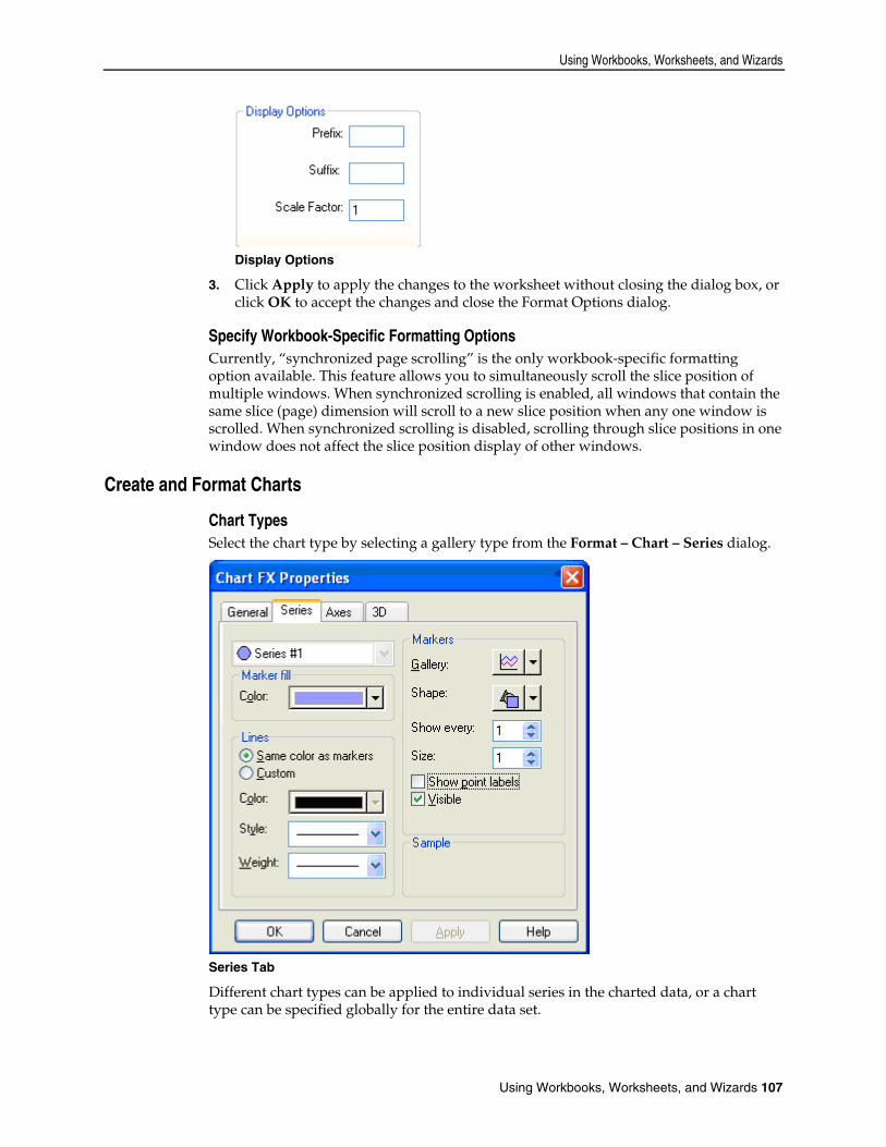
Using Workbooks, Worksheets, and Wizards
Using Workbooks, Worksheets, and Wizards 107
Display Options
3. Click Apply to apply the changes to the worksheet without closing the dialog box, or click OK to accept the changes and close the Format Options dialog.
Specify Workbook-Specific Formatting Options Currently, “synchronized page scrolling” is the only workbook-specific formatting option available. This feature allows you to simultaneously scroll the slice position of multiple windows. When synchronized scrolling is enabled, all windows that contain the same slice (page) dimension will scroll to a new slice position when any one window is scrolled. When synchronized scrolling is disabled, scrolling through slice positions in one window does not affect the slice position display of other windows.
Create and Format Charts
Chart Types Select the chart type by selecting a gallery type from the Format – Chart – Series dialog.
Series Tab
Different chart types can be applied to individual series in the charted data, or a chart type can be specified globally for the entire data set.

Workbook and Worksheet Procedures
108 Oracle Retail Predictive Application Server
When you select a chart type from the Gallery menu, drag your cursor over the chart type images.
The name of each chart type will appear in the text field at the bottom of the menu. The Chart FX charting utility provides the following available chart types (and their descriptions): Line – Line shows trends or changes in data over a period of time. Each data point in
the series is connected with a line. Area – Area shows the relative importance of values over a period of time. Each data
point in the series is connected with a line, and the area beneath this line is shaded. Curve – Curve is similar to a line chart, but the lines curve to smoothly pass through
each point or data marker. Area-Curve – Area-Curve is a combination of the Area chart type and the Curve
chart type. Each data point in the series is connected with a smooth, curving line, and the area beneath the curve is shaded.
Step – Step is similar to a line chart, but only vertical and horizontal line segments connect the data points in a series. The resulting graph appears as stair steps.
Scatter – Scatter is a point chart that shows the relationship or degree of relationship between numeric values in several series, or it plots two groups of numbers as one series of x-y coordinates.
Bubble – Bubble plots a set of values with one of the values specifying the size of the bubble marker. If two data series are plotted, values in the first series specify the position (height) of the bubble marker along the y-axis, and the corresponding values in the second series specify the size of the bubble marker drawn at each position. If three data series are plotted, values in the first two series define the (x,y) coordinates of the bubble marker, and the corresponding values of the third series specify the bubble marker volume.
Bar – Bar shows variation between data sets by depicting series as bars stretching vertically towards the top of the chart window.
Gantt – Gantt is basically a horizontal version of a bar chart. This chart type shows variation between data sets by depicting series as bars stretching horizontally across the chart window. Gantt charts are commonly used to track activities over time.
Cube – Cube is similar to a bar chart, but a cube is displayed at the proper height instead of a complete bar.
Candlestick – Candlestick is a chart that is typically used in financial areas, as related to stock prices.
Open-High-Low-Close – Open-High-Low-Close is a chart that is typically used in financial areas, as related to stock prices. Each marker is defined by four series that represent a stock’s opening, high, low, and closing prices.

Using Workbooks, Worksheets, and Wizards
Using Workbooks, Worksheets, and Wizards 109
High-Low-Close – High-Low-Close is a chart that is typically used in financial areas, as related to stock prices. Each marker is defined by three series that represent a stock’s high, low, and closing prices.
Pie – Pie shows the relationship or proportions of parts to a whole. Percentages of the whole for each piece of the pie are calculated and displayed in the chart.
Doughnut – Doughnut is the same as a pie chart, but with a hole in the center. Pareto – Pareto is a chart that is often used in statistical areas. Bars show a variation
over a period of time, and a cumulative curve indicates the proportion accumulated by each column in the chart.
Pyramid – Pyramid shows the relationship of parts to a whole in the format of a pyramid. Different point values in the series are represented by different colors and levels in the pyramid.
Radar – Radar plots values in polar coordinates and shows the relative importance of values over a period of time.
Contour/Spectral – Contour/Spectral is basically a line chart with different colors assigned to different ranges beneath the plotted values. This depends on each point height (y value). The contour plot is displayed in a 2D representation.
Surface – Surface is basically a line chart with different colors assigned to different ranges beneath the plotted values. This depends on each point height (y value). The surface plot is usually displayed in a 3D representation.
Change the Chart Type
Note: You must be in chart view in order to display the Chart FX dialog box. If you are in grid view, click the Toggle button before you proceed.
Toggle Button
Navigate From the Format menu, select the Chart option, or click Format on the toolbar. The Chart FX Properties dialog box displays.

Workbook and Worksheet Procedures
110 Oracle Retail Predictive Application Server
Chart F/X Properties Dialog Box
1. Select the Series tab. 2. Click the Gallery arrow to produce a menu of available gallery types.
Note: You can change the chart type for an individual data series by selecting that series’ name from the series pick list at the top left of the dialog. If <All Series> is selected, the gallery type you choose will affect the entire chart format.
3. Click the desired chart type. To identify the chart types in the gallery menu, drag your cursor over the chart type images. The name of each chart type appears in the text field at the bottom of the menu.
4. Click OK.
Show/Hide Legends in a Chart You can toggle the display of both the series legend and the values legend in your chart. The series legend identifies the collection of data represented by each plotted series in your chart. The values legend, also called the point legend, identifies the units displayed along the x-axis of your chart. For example, if your chart displays the calendar hierarchy along the x-axis, the values legend would identify the week or month indicated at each point.
Hide a Currently Displayed Legend 1. Right-click on the legend to be hidden. A Chart FX quick menu appears. 2. Select Hide.
Note: When the values legend (point legend) is hidden, the values that correspond to each x-axis point are displayed directly on the chart.

Using Workbooks, Worksheets, and Wizards
Using Workbooks, Worksheets, and Wizards 111
Show a Currently Hidden Legend 3. Click Tools on the Chart FX toolbar.
Tools Button
Note: If the Chart FX toolbar is currently hidden, display it by right-clicking within the chart display area and selecting the Toolbar option from the quick menu.
4. Perform the following as needed: Select Values Legend to redisplay the values legend (point legend). Select Series Legend to redisplay the series legend.
5. You can toggle the display of both the series legend and the values legend in your chart.
6. The series legend identifies the collection of data represented by each plotted series in your chart.
7. The values legend, also called the point legend, identifies the units displayed along the x-axis of your chart. For example, if your chart displays the calendar hierarchy along the x-axis, the values legend identifies the week or month indicated at each point.
Resize Chart and Legend Display Areas To resize the chart and legend display areas, position the cursor immediately over a divider line between the chart display and legend display area. When the appearance of the cursor changes; click and hold the divider line, drag the line to any position you choose, and release the mouse button. The chart display and the affected legend are redrawn to reflect the new boundaries. You can perform this same function at the edge of the chart box (the area within the chart axes). Drag this boundary to increase or decrease the size of the chart.
Title a Chart Choose one of the following two methods to create a chart title that will appear immediately above the chart display:
Method 1
Navigate From the Format menu, select the Chart option, or click Format on the toolbar. On the General tab of the Chart FX Properties dialog, enter a title for your chart in the Title text field, and click OK.
Method 2 1. Right-click anywhere within the main chart display to produce the Chart FX quick
menu. 2. Select Edit Title. 3. Type or edit the title for your chart in the text box.
Change the Font, Font Style, Font Size, and Color of Chart Text Access the Chart FX right-click menu to change the format of text in your chart. Text can be changed in chart areas; such as the chart title, chart axes, axis titles, point labels, series legend, and point legend.
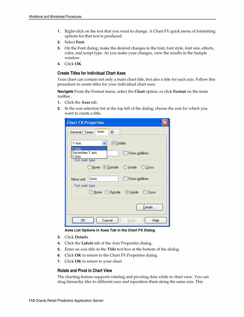
Workbook and Worksheet Procedures
112 Oracle Retail Predictive Application Server
1. Right-click on the text that you want to change. A Chart FX quick menu of formatting options for that text is produced.
2. Select Font. 3. On the Font dialog; make the desired changes to the font, font style, font size, effects,
color, and script type. As you make your changes, view the results in the Sample window.
4. Click OK.
Create Titles for Individual Chart Axes Your chart can contain not only a main chart title, but also a title for each axis. Follow this procedure to create titles for your individual chart axes:
Navigate From the Format menu, select the Chart option, or click Format on the main toolbar.. 1. Click the Axes tab. 2. In the axis selection list at the top left of the dialog, choose the axis for which you
want to create a title.
Axes List Options in Axes Tab in the Chart FX Dialog
3. Click Details . 4. Click the Labels tab of the Axis Properties dialog. 5. Enter an axis title in the Title text box at the bottom of the dialog. 6. Click OK to return to the Chart FX Properties dialog. 7. Click OK to return to your chart.
Rotate and Pivot in Chart View The charting feature supports rotating and pivoting data while in chart view. You can drag hierarchy tiles to different axes and reposition them along the same axis. This

Using Workbooks, Worksheets, and Wizards
Using Workbooks, Worksheets, and Wizards 113
function is performed in the same manner that it is in grid view. When hierarchy tiles are repositioned in chart view, the new arrangement of hierarchies is preserved in the grid view of that same data.
Tip: Use the New Window feature on the Window menu to simultaneously view: Grid mode data that is based on one arrangement of hierarchy tiles AND chart mode data that is based on a different arrangement.
Change Data Values within a Chart The charting feature allows you to change data values directly while in chart mode. You are not required to toggle back to grid mode to manually enter new data values.
Note: Only writable measures can be changed in either chart mode or grid mode. Data points corresponding to read-only measures cannot be dragged and dropped.
Alternatively, you can open the Chart FX Data Editor to manually enter exact data values while in chart mode. The Data Editor is an editable data grid that contains the values of the elements plotted in your chart. You can double-click any writable data value in the grid to edit it. The chart is instantly redrawn to reflect your change.
Change Data Values by "Hot Charting" "Hot charting" is the process of amending data values by dragging and dropping data points in the chart. 1. Click and hold the data point that you want to edit. 2. With the mouse button depressed, drag the data point to its new location. As you
move the data point, balloon text expands to indicate the y-axis value nearest the point’s current location.
Note: If the point labels feature is toggled on, the point label changes to indicate the current value of the data point.
3. Release the mouse button to drop the point in the appropriate location.
Display a Chart in 3D View Follow this procedure to change your chart from a two-dimensional to a three-dimensional view.
Navigate From the Format menu, select Chart. 1. Click General. 2. In the Effects portion of the dialog, select the 3D option to display your chart in
three-dimensional mode. Clear the check box to display your chart two-dimensionally.
3. Click OK. If you switch to a three-dimensional view of your chart, the system will display your data in standard 3D view. You have the option to manipulate certain aspects of this 3D view (for instance, rotation angles, shadowing, depth, and perspective) to create a customized three-dimensional chart.
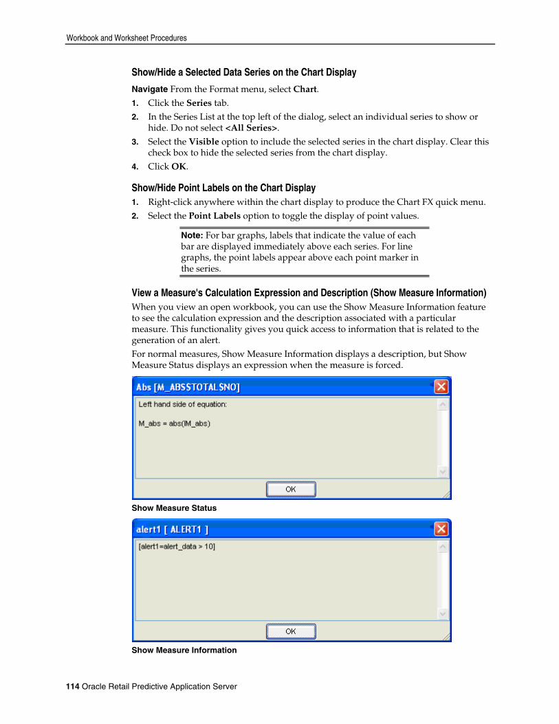
Workbook and Worksheet Procedures
114 Oracle Retail Predictive Application Server
Show/Hide a Selected Data Series on the Chart Display
Navigate From the Format menu, select Chart. 1. Click the Series tab. 2. In the Series List at the top left of the dialog, select an individual series to show or
hide. Do not select <All Series>. 3. Select the Visible option to include the selected series in the chart display. Clear this
check box to hide the selected series from the chart display. 4. Click OK.
Show/Hide Point Labels on the Chart Display 1. Right-click anywhere within the chart display to produce the Chart FX quick menu. 2. Select the Point Labels option to toggle the display of point values.
Note: For bar graphs, labels that indicate the value of each bar are displayed immediately above each series. For line graphs, the point labels appear above each point marker in the series.
View a Measure's Calculation Expression and Description (Show Measure Information) When you view an open workbook, you can use the Show Measure Information feature to see the calculation expression and the description associated with a particular measure. This functionality gives you quick access to information that is related to the generation of an alert. For normal measures, Show Measure Information displays a description, but Show Measure Status displays an expression when the measure is forced.
Show Measure Status
Show Measure Information

Using Workbooks, Worksheets, and Wizards
Using Workbooks, Worksheets, and Wizards 115
For alert measures, Show Measure Information and Show Measure Status both show an expression. The Show Measure Information comes from the Description field, and the Show Measure Status is output from the Rule Engine. 1. Right-click the measure’s label in the measure axis of your worksheet. 2. On the quick menu, select Show Measure Information. 3. View the calculation and measure description information in the Measure Info
dialog. 4. Click OK.
Using Wizards
Wizards The basic purpose of wizards is to allow you to select specific data to be incorporated into your new workbook. The new workbook wizard will walk you through the process of creating a new workbook from a template. A wizard is an automated feature that prompts you for answers to a series of questions. It then uses your answers to format the workbook that you want to create. The specific questions depend on the type of workbook being built. Wizards are also used by the system to gather required information related to various administrative, analyses, planning, and forecasting processes. For example, wizards are in place to aid System Administrators in the task of adding and deleting system users, and to aid users in the process of defining and editing alerts. Whenever user input is required by the system to conduct a particular task, wizards are the interface through which the system collects the necessary information.
Typical Wizards Encountered when Using RPAS New workbook creation wizards – This wizard prompts you for information
regarding the contents and layout of new workbooks. Your system may contain workbook template wizards for Administration workbooks, Analysis workbooks, Planning workbooks, and/or Forecasting workbooks.
Alert Builder wizard – This wizard is used to define how user-created measures are to be evaluated during the alert generation process.
User Administration wizard – This wizard is used by System Administrators to add/delete system users, add/delete user groups, and change user passwords and settings.
How Wizards are Invoked and Navigated To access a new workbook wizard for a template:
Navigate From the File menu, select New. 1. Select a workbook template. 2. Proceed through the wizard screens. Make the appropriate selections on each screen,
and click Next to advance. 3. Click Back to change information that was selected on a previous screen. 4. Click Finish when you reach the final wizard screen, which is indicated when Next is
no longer enabled. The system will assimilate all wizard selections made and format and build your new workbook.

Using Wizards
116 Oracle Retail Predictive Application Server
Wizard AutoFinish Each time you complete the required information on a wizard screen, click the Next button to advance to the next screen. Notice that the Finish button is also enabled at most stages in the wizard process. As an alternative means of completing a wizard, you may click the Finish button to have the system automatically complete the wizard process, which is based on stored selection data. Dialog screens in wizards automatically reflect the selections made the last time the wizard was successfully completed. Before building a new workbook, the system creates a record of the choices made on each wizard screen. The system maintains this record of the most recent selections. Therefore, enough "default" information is generally present for the system to build a new workbook without requiring you to access every dialog within the wizard. The Finish button is enabled to allow you to instruct the system to build a new workbook or to perform a process that is based on the most recent information it has stored for a given workbook template. Whenever the Finish button is pressed, the system automatically processes the remaining wizard screens, and it accepts whatever selections are currently stored for each dialog. If the system encounters a screen where a valid selection does not exist (requiring user input), the AutoFinish process is interrupted. At this point, the dialog in question is displayed, and you are required to enter the appropriate information before the Next and Finish buttons become enabled.
Wizard Two-Tree Selection Dialogs One very common type of wizard screen you will encounter is the two-tree selection dialog. On this type of screen, you are asked to pick items (such as products or time periods) from a list of Available items and move them to a list of Selected items. Only items in the Selected items list will be incorporated into the new workbook. Selection dialogs in new workbook wizards automatically reflect the product, location, and time period selections made the last time that wizard was used to build a new workbook. For example, suppose that you are building a new Forecast Maintenance Workbook in Oracle Retail Demand Forecasting. The list of products chosen in the product selection dialog of this wizard automatically appears on the Selected Products side of the product selection dialog the next time you build a new Forecast Maintenance Workbook. Of course, you can still select and de-select products as desired; the automatic pre-selection process is intended to provide you with a logical selection starting point based on the most recent items of interest.
Wizard Procedures
Single-Selection Wizards All of the screens that you encounter in the wizard process are of the single-select variety. Single-select wizard dialogs require you to make a selection from a single list of options.
Select Options from Single-Select Dialogs When only one choice is allowed for a short list of options, radio buttons are used to force a single selection. Click the radio button that corresponds to your preference, and click Next to proceed to the next screen. If there is a long list of available options, a selection list (rather than radio buttons) is provided. Click on your desired option to highlight it, and click Next to proceed.

Using Workbooks, Worksheets, and Wizards
Using Workbooks, Worksheets, and Wizards 117
Wizard Two-Tree Selection Lists The wizards in the Oracle Retail Predictive Solutions frequently use selection lists. Selection lists allow you to select values from one list and move them into another. Use these lists to assign contents to workbooks.
Select or Move Items on a Wizard Two-Tree Selection Dialog Use the following instructions to move hierarchy items from the Available list into the Selected list or to move items from the Selected list back into the Available list. Only those items in the Selected items list will be incorporated into the workbook. 1. Check the boxes next to the items that you want to move to the Selected list. The
corresponding items are displayed in the Selected list. 2. To remove items from the Selected list, uncheck the boxes next to the corresponding
items in the Available list. 3. After you finish selecting items, click Next or Finish.
Add All Items from a Wizard’s List of Available Items 1. Right-click on the Available list (left side). 2. Select Add All.
Remove All Items from a Wizard’s List of Selected Items 1. Right-click on the Available list (left side). 2. Select Remove All.
Collapse a Node or Expand a Branch on a Wizard Two-Tree List
Note: The Collapse Node and Expand Branch options are available only when you right-click on a node that is not base level.
Collapse a Node on a Wizard List
1. Right-click on a non-base level node in a wizard list. 2. Select (left-click on) Collapse Node.
Expand a Collapsed Node on a Wizard List
1. Right-click on the collapsed node. 2. Select (left-click on) Expand Branch.
Collapse or Expand an Entire Dimension on a Wizard Two-Tree List
Navigate From a wizard two-tree selection dialog, right-click on a wizard list (Available or Selected). On the menu that appears, all dimensions available for display are listed beneath the Find option. Currently expanded dimensions are indicated by checkmarks. 1. To expand a collapsed dimension (has no checkmark), click on its label. 2. To allow dimensions not on the list to be expanded, select a higher level for hierarchy
rollup.

Using Wizards
118 Oracle Retail Predictive Application Server
Collapse or Expand Multiple Dimensions on a Wizard Two-Tree List
Navigate From a wizard two-tree selection dialog, right-click on a wizard list (Available or Selected). 1. Select (left-click) Select Dimensions. 2. In the Select Dimensions dialog box, highlight each dimension that you want to
display in your worksheet. Make sure that all dimensions that you want to remain collapsed in your worksheet view are left unselected.
3. Click OK. 4. To allow dimensions not on the list to be expanded or collapsed, select a higher level
for hierarchy rollup.
Select a Higher Level for a Hierarchy Rollup
Navigate From a wizard two-tree selection dialog, right-click on a wizard list (Available or Selected). From the menu that displays, choose Select Rollup and the highest dimension that you want to display. You can streamline the process of item selection in wizards by saving lists of selections so that the same set can be instantly applied to any applicable two-tree selection dialog. Saving and loading complete lists of commonly selected items reduces the time required to build new workbooks. This is because it eliminates the need to re-select combinations of items over time or across workbook templates.
Find an Item on a Wizard Two-Tree List 1. Right-click any item on a wizard two-tree selection list. 2. Left-click Find to select it. 3. Under Find What, type all or part of the name of the item to find. The wizard will
attempt to find the item as you type. Only the list that you right-clicked (Available or Selected) will be searched.
You can select the Match Case or the Match Entire Description check boxes to further limit your search. If necessary, click Repeat Find to locate the next matching occurrence. Dimension labels, if displayed, are dynamic headers that appear at the top of each wizard list (Available or Selected). Each label indicates the dimension that appears in the column beneath it, and the labels can be used to quickly collapse or expand the dimension that they represent.
Show/Hide Dimension Labels in Wizard Two-Tree Lists Dimension labels are dynamic headers that, if displayed, appear at the top of each wizard list (Available or Selected). Each label indicates the dimension appearing in the column beneath it, and the labels can be used to quickly collapse or expand the dimension that they represent. 1. On a wizard two-tree dialog, right-click on a list (Available or Selected). 2. The Show Connector Lines option toggles (on and off) the connector lines that
indicate hierarchical relationships on the list. A checkmark indicates that the lines are shown.
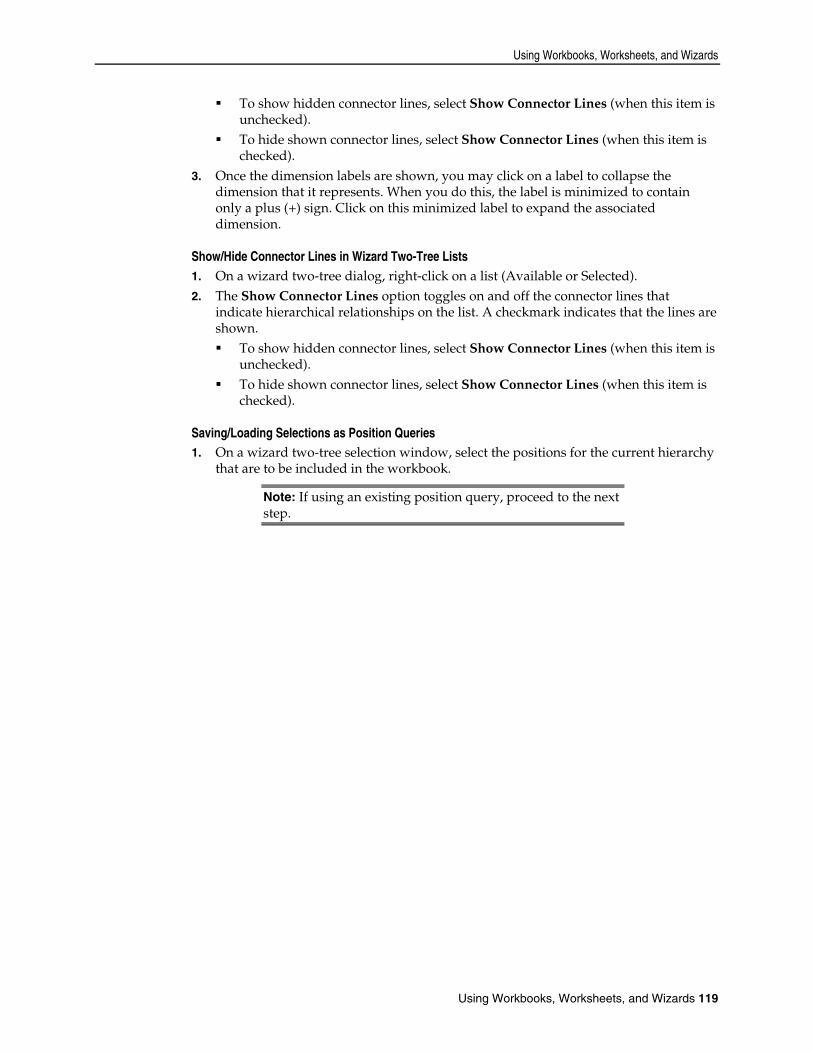
Using Workbooks, Worksheets, and Wizards
Using Workbooks, Worksheets, and Wizards 119
To show hidden connector lines, select Show Connector Lines (when this item is unchecked).
To hide shown connector lines, select Show Connector Lines (when this item is checked).
3. Once the dimension labels are shown, you may click on a label to collapse the dimension that it represents. When you do this, the label is minimized to contain only a plus (+) sign. Click on this minimized label to expand the associated dimension.
Show/Hide Connector Lines in Wizard Two-Tree Lists 1. On a wizard two-tree dialog, right-click on a list (Available or Selected). 2. The Show Connector Lines option toggles on and off the connector lines that
indicate hierarchical relationships on the list. A checkmark indicates that the lines are shown. To show hidden connector lines, select Show Connector Lines (when this item is
unchecked). To hide shown connector lines, select Show Connector Lines (when this item is
checked).
Saving/Loading Selections as Position Queries 1. On a wizard two-tree selection window, select the positions for the current hierarchy
that are to be included in the workbook.
Note: If using an existing position query, proceed to the next step.
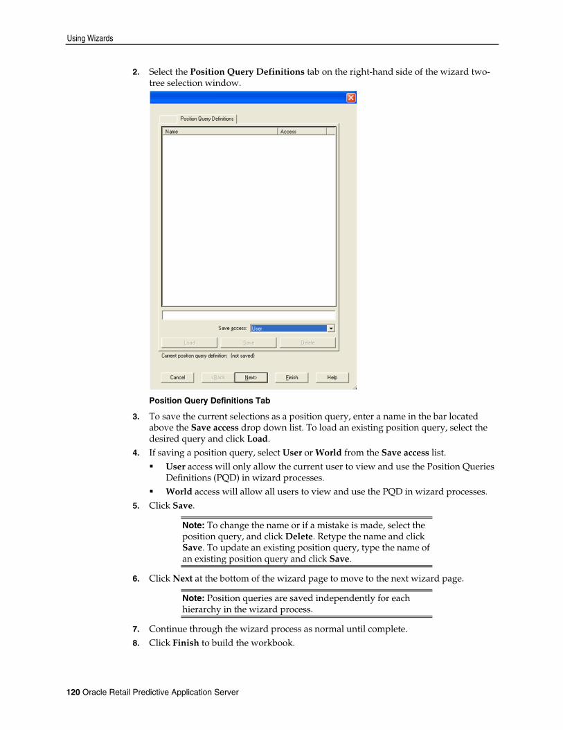
Using Wizards
120 Oracle Retail Predictive Application Server
2. Select the Position Query Definitions tab on the right-hand side of the wizard two-tree selection window.
Position Query Definitions Tab
3. To save the current selections as a position query, enter a name in the bar located above the Save access drop down list. To load an existing position query, select the desired query and click Load.
4. If saving a position query, select User or World from the Save access list. User access will only allow the current user to view and use the Position Queries
Definitions (PQD) in wizard processes. World access will allow all users to view and use the PQD in wizard processes.
5. Click Save.
Note: To change the name or if a mistake is made, select the position query, and click Delete. Retype the name and click Save. To update an existing position query, type the name of an existing position query and click Save.
6. Click Next at the bottom of the wizard page to move to the next wizard page.
Note: Position queries are saved independently for each hierarchy in the wizard process.
7. Continue through the wizard process as normal until complete. 8. Click Finish to build the workbook.
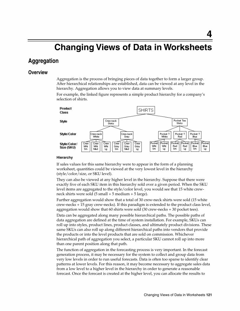
Changing Views of Data in Worksheets 121
4 Changing Views of Data in Worksheets
Aggregation
Overview Aggregation is the process of bringing pieces of data together to form a larger group. After hierarchical relationships are established, data can be viewed at any level in the hierarchy. Aggregation allows you to view data at summary levels. For example, the linked figure represents a simple product hierarchy for a company’s selection of shirts.
Hierarchy
If sales values for this same hierarchy were to appear in the form of a planning worksheet, quantities could be viewed at the very lowest level in the hierarchy (style/color/size, or SKU level). They can also be viewed at any higher level in the hierarchy. Suppose that there were exactly five of each SKU item in this hierarchy sold over a given period. When the SKU level items are aggregated to the style/color level, you would see that 15 white crew-neck shirts were sold (5 small + 5 medium + 5 large). Further aggregation would show that a total of 30 crew-neck shirts were sold (15 white crew-necks + 15 gray crew-necks). If this paradigm is extended to the product class level, aggregation would show that 60 shirts were sold (30 crew-necks + 30 pocket tees). Data can be aggregated along many possible hierarchical paths. The possible paths of data aggregation are defined at the time of system installation. For example, SKUs can roll up into styles, product lines, product classes, and ultimately product divisions. These same SKUs can also roll up along different hierarchical paths into vendors that provide the products or into the level products that are sold on commission. Whichever hierarchical path of aggregation you select, a particular SKU cannot roll up into more than one parent position along that path. The function of aggregation in the forecasting process is very important. In the forecast generation process, it may be necessary for the system to collect and group data from very low levels in order to run useful forecasts. Data is often too sparse to identify clear patterns at lower levels. For this reason, it may become necessary to aggregate sales data from a low level to a higher level in the hierarchy in order to generate a reasonable forecast. Once the forecast is created at the higher level, you can allocate the results to

Aggregation
122 Oracle Retail Predictive Application Server
whatever lower level you want. This is done through the process of spreading, which is discussed in the overview of spreading topic. Aggregation is also important in the plan approval process. Typically, you would not want to approve sales plans at the SKU/Week level. This level of approval might be very time-consuming if hundreds of thousands of SKUs were involved. Sales plan figures are usually aggregated to a higher level, such as Style/Month, for approval.
Data Aggregation in a Worksheet When viewing quantitative data in a worksheet, you may require a view of the information at a more aggregate level. The Oracle Retail Predictive Solutions use the hierarchical structure defined by your organization to roll up information for presentation at a higher level. Rollup is the path that the system follows from the root of the hierarchy to another higher dimension in the hierarchy during the aggregation process. There are several ways to obtain views of the data at these higher levels. Regardless of the method you choose, you must first select the highest dimension level that you want to see within the rollup path that you want to use. To do this, properly positioning the cursor, and click the right mouse button. Then select the Select Rollup option from the quick menu. The quick menu associated with a given hierarchy can be accessed when the cursor is positioned over that hierarchy’s axis in the grid. For example, to select the rollup for the product hierarchy: 1. Position the cursor over any point in the axis where the product hierarchy is
displayed. 2. Right-click the mouse to obtain the associated quick menu. 3. Choose Select Rollup, and select the highest dimension to be displayed.
Data Aggregation in Outline View The following discussion about data aggregation options is most applicable when you view your worksheet data in block mode. This is because block mode only allows the display of data values at one dimensional level at a time (the lowest level currently expanded in the grid). The following procedures effectively collapse lower-level dimensions, which results in the aggregation of data to the next higher level. When you view your worksheet in outline view, the display lets you see data at multiple dimensional levels at the same time, so you do not need to collapse lower-level dimensions to see aggregate totals for higher levels. The menu items described below are still useful for manipulating the display (collapsed vs. expanded) of various dimensional levels for the data hierarchies in your worksheet.
Aggregation Options You can choose any of the following three methods to aggregate your data and view it at the higher level. To access these options, right-click any worksheet axis and a quick menu will be displayed. The following are the options that enable aggregation.

Changing Views of Data in Worksheets
Changing Views of Data in Worksheets 123
Right-Click Menu Showing Dimension List and Other Options
Dimension List Options The Dimension List option allows you to expand or collapse the display of one dimension at a time. When a worksheet dimension is collapsed from the grid display, all of that dimension’s associated data are aggregated to the next higher level that is currently displayed. These are the options: all(Location) Region District Store
Note: These options will vary depending on the hierarchy and dimension positions in the worksheet.
To aggregate data using the Dimension List option: 1. Right-click any worksheet axis to display a quick menu of options that are relevant to
that hierarchy. Dimensions that are currently displayed are shown in the dimension list with checkmarks beside them.
Note: If you want to aggregate data to a dimension higher than those shown in the dimension list, you must first use the Select Rollup option to specify the highest dimension that you want to see.

Aggregation
124 Oracle Retail Predictive Application Server
2. Click any currently checked dimension to collapse that hierarchical level. All associated data will be aggregated to the next higher dimension that is displayed.
Note: Clicking any unchecked dimension in the list causes the reverse process to happen. The previously collapsed dimension will be displayed in the grid in its proper relative location in the hierarchy.
Select Dimensions Option The Select Dimensions option allows you to simultaneously expand or collapse the display of multiple dimensions. Select this option to display a dialog box where you can select the exact dimensions that you want displayed in your worksheet. To aggregate data using the Select Dimensions option: 1. Right-click any worksheet axis to display a quick menu of options that are relevant to
that hierarchy. 2. Select the Select Dimensions option. 3. On the dialog that opens, select all dimensions that you want to display in your
worksheet. Highlighted dimensions will appear in the display. Non-highlighted dimensions will be collapsed and data will be aggregated to the next higher level.
4. Click OK.
Show Dimension Labels Option The Show Dimension Labels option is useful when you want to expand or collapse dimensions repeatedly, and if you want to avoid accessing the quick menu each time you do it. This option toggles the display of cursor-sensitive dimension header labels in your worksheet. When you click on the label for a particular dimension, that dimension is collapsed in the grid, and all associated data is aggregated to the next higher level. Once the dimension header labels are activated, dimensions can be expanded or collapsed in one single click. To aggregate data using the Show Dimension Labels option: 1. Right-click any worksheet axis to display a quick menu of options relevant to that
hierarchy. 2. Select the Show Dimension Labels option. Minimized tabs display, which is located
at the left side of the column axis headings or at the top of the row axis headings, depending on your axis selection..
3. Place the cursor over these tabs. The tabs expand to display the dimension labels. 4. Click any dimension label to collapse that dimension in the grid and aggregate the
data to the next higher level.
Note: Labels representing collapsed dimensions contain a plus (+) sign. Click the plus sign to maximize the label and expand that dimension in the grid.
Display Worksheet Data in Chart Form Displaying worksheet data in chart form is a useful feature in worksheets. Any numeric data or subset of data in a worksheet can easily be converted to a chart format. Viewing data in a graphical format can enable users to subjectively assess (at a glance) how well system and final forecasts have predicted actual sales values. Charts can be used for many other purposes, such as graphically illustrating changes in sales and forecast
Changing Views of Data in Worksheets
Changing Views of Data in Worksheets 125
patterns over time. Patterns and trends in data can be recognized much quicker when data is presented in the form of a chart than when that same data is shown in spreadsheet form.
Customizing Chart Content You can place as much or as little information as necessary in charts. Select the data cells in the grid that you want to see charted. When you toggle your worksheet view to chart mode, only the selected information is extracted from the grid and plotted in your chart. Like grid-format worksheets, you can save and commit charts as components of the workbook. The data that they contain can be printed and/or exported for use in other systems. Also, by using the New Window option on the Window menu, you can simultaneously view workbook data in grid mode and chart mode.
Customizing Chart Format In addition to customizing content, you can customize the various attributes of a chart’s format: You can choose the type of the chart (for instance; bar graph, line graph, and pie
chart) and switch between chart types. You can specify the color scheme for your chart; including selections for individual
data series, the chart background, the legend, and the chart area. You can specify the content and style of the chart title. You can specify customized axis settings; such as the major and minor axis units, the
axis scale, and the individual axis titles. You can switch between a two-dimensional and a three-dimensional view of your
charted data. You can control features; such as shadowing, depth, and perspective of your 3D
chart.
Chart Styles Specific combinations of chart formatting options can be saved as chart styles. These saved styles can be applied to subsequent collections of data, which eliminates the need to manually format each new chart to your specifications.
Rotating and Pivoting Chart Data The charting feature supports the rotation and pivoting of data while in chart view. Hierarchy tiles can be dragged to different axes and repositioned in the same manner that it is performed in grid view. Rotating and pivoting can facilitate data analysis by providing different views of the same data.
Changing Data Values in a Chart You can directly change data values while in chart mode. You are not required to toggle back to grid view to manually key in new data values. These values can be amended by dragging and dropping data points in the chart.
Pivoting Data Pivoting is similar to rotating, but only one axis is involved. Pivoting occurs when two or more hierarchy tiles that reside on the same axis change their order on the worksheet. To pivot data, drag and drop one hierarchy tile in front of the other. The same cursor indicators that are used in rotating data are also used when pivoting data.
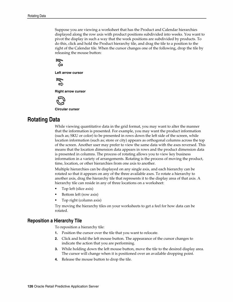
Rotating Data
126 Oracle Retail Predictive Application Server
Suppose you are viewing a worksheet that has the Product and Calendar hierarchies displayed along the row axis with product positions subdivided into weeks. You want to pivot the display in such a way that the week positions are subdivided by products. To do this, click and hold the Product hierarchy tile, and drag the tile to a position to the right of the Calendar tile. When the cursor changes one of the following, drop the tile by releasing the mouse button:
Left arrow cursor
Right arrow cursor
Circular cursor
Rotating Data While viewing quantitative data in the grid format, you may want to alter the manner that the information is presented. For example, you may want the product information (such as; SKU or color) to be presented in rows down the left side of the screen, while location information (such as; store or city) appears as orthogonal columns across the top of the screen. Another user may prefer to view the same data with the axes reversed. This means that the location dimension data appears in rows and the product dimension data is presented in columns. The process of rotating allows you to view key business information in a variety of arrangements. Rotating is the process of moving the product, time, location, or other hierarchies from one axis to another. Multiple hierarchies can be displayed on any single axis, and each hierarchy can be rotated so that it appears on any of the three available axes. To rotate a hierarchy to another axis, drag the hierarchy tile that represents it to the display area of that axis. A hierarchy tile can reside in any of three locations on a worksheet: Top left (slice axis) Bottom left (row axis) Top right (column axis)
Try moving the hierarchy tiles on your worksheets to get a feel for how data can be rotated.
Reposition a Hierarchy Tile To reposition a hierarchy tile: 1. Position the cursor over the tile that you want to relocate. 2. Click and hold the left mouse button. The appearance of the cursor changes to
indicate the action that you are performing. 3. While holding down the left mouse button, move the tile to the desired display area.
The cursor will change when it is positioned over an available dropping point. 4. Release the mouse button to drop the tile.
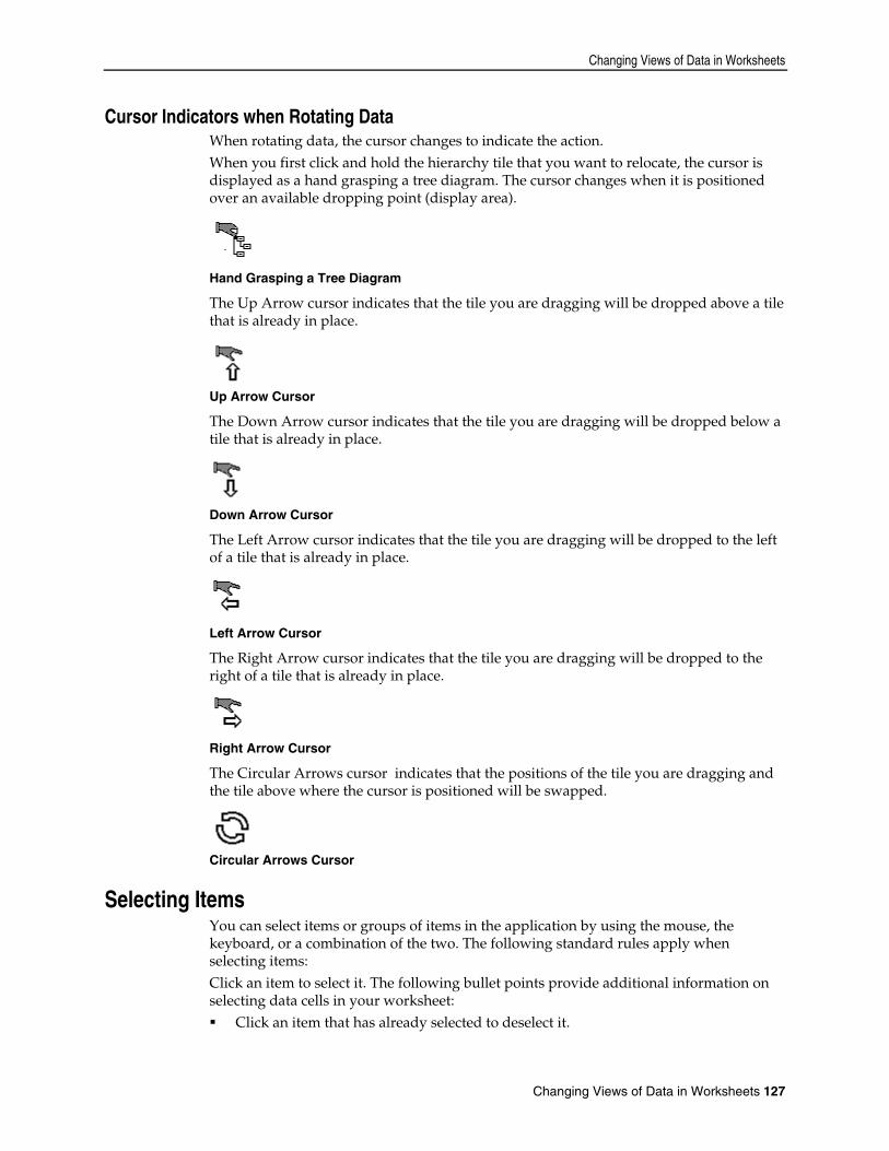
Changing Views of Data in Worksheets
Changing Views of Data in Worksheets 127
Cursor Indicators when Rotating Data When rotating data, the cursor changes to indicate the action. When you first click and hold the hierarchy tile that you want to relocate, the cursor is displayed as a hand grasping a tree diagram. The cursor changes when it is positioned over an available dropping point (display area).
Hand Grasping a Tree Diagram
The Up Arrow cursor indicates that the tile you are dragging will be dropped above a tile that is already in place.
Up Arrow Cursor
The Down Arrow cursor indicates that the tile you are dragging will be dropped below a tile that is already in place.
Down Arrow Cursor
The Left Arrow cursor indicates that the tile you are dragging will be dropped to the left of a tile that is already in place.
Left Arrow Cursor
The Right Arrow cursor indicates that the tile you are dragging will be dropped to the right of a tile that is already in place.
Right Arrow Cursor
The Circular Arrows cursor indicates that the positions of the tile you are dragging and the tile above where the cursor is positioned will be swapped.
Circular Arrows Cursor
Selecting Items You can select items or groups of items in the application by using the mouse, the keyboard, or a combination of the two. The following standard rules apply when selecting items: Click an item to select it. The following bullet points provide additional information on selecting data cells in your worksheet: Click an item that has already selected to deselect it.

Spreading
128 Oracle Retail Predictive Application Server
To use the mouse to select a group of contiguous items, position the mouse cursor over the first item in the group. a. Press and hold the left mouse button. b. Drag the cursor to the last element in the group. c. Release the mouse button.
To select a group of contiguous items, select one position with the mouse and hold down the Shift key while choosing another position. This process selects the first item, the last item, and any positions in between.
To select a group of items that are not contiguous, hold down the Ctrl key, and click any required positions.
Use the spacebar to toggle the selection of the last active item.
Selecting Items in a Wizard List Selection of products, locations, and time periods to be included in a workbook is often required when particular workbook wizards are accessed. Products, locations, and time periods on the Available side of the wizard must be highlighted and moved to the Selected side of the wizard for inclusion in a workbook.
Selecting Items in the Grid Cells or groups of cells must be selected in the grid before certain operations can be performed on them. Operations like cutting and copying data, filling or clearing data cells, and displaying data in chart form are typically performed on a subset of worksheet cells that you must select prior to invoking the menu command. There are several ways to select cells in the grid. In general, cell selections should be made in the worksheet axes (where the column and row headers appear), and not in the cells. To select one cell; click the column header that corresponds to the cell, and click the
corresponding row label. When no selections exist, click on any column header in the column axis to
automatically select that entire column. The same is true for selections made in the row axis. Selection of a particular row header results in the selection of the entire row. When selections simultaneously exist in the column axis and in the row axis, any cells located at that row/column intersection will be selected in the grid. The selection rules outlined above, such as using the Shift and Ctrl keys to select multiple items, can be applied in the axis headers to isolate groups of cells.
If you want to select a block of contiguous cells, the following method allows you to make your selection within the grid. a. Click in the topmost, leftmost cell in the block to be selected. b. Hold down the mouse button, and drag the cursor to the bottommost, rightmost
cell, and release the mouse button. c. As you drag the mouse, the corresponding column header and row header
positions are automatically selected according to your actions.
Spreading Spreading (the opposite of aggregation) allows you to view data at more detailed levels. In spreading, totals at higher level dimensions are allocated to lower level dimensions, which are based on the lower level’s relationship to the total.

Changing Views of Data in Worksheets
Changing Views of Data in Worksheets 129
Spreading Aggregate Forecast Values When data is too sparse to create useful forecasts at a low level, it can be aggregated to a summary level. The system spreads forecast totals at this higher level back down to the lower level, which is based on the lower level’s percent contribution to the higher. The data at the lowest level in the hierarchy may be too sparse to create a meaningful forecast; however, this same data can be very useful in determining the percent contribution that each position in the lower level makes toward the higher level. For example, an aggregate-level class/store forecast predicts 50 shirts to be sold in Store #001 over a given time period. A forecast at the lower SKU/store level also determines that red shirts make up 40% of the demand, blue shirts make up 30%, white shirts make up 20%, and black shirts make up 10%. These percentages can be used to spread the total of 50 shirts back down to the lower level of color. For example, an aggregate-level class/store forecast predicts 50 shirts to be sold in Store #001 over a given time period. A forecast at the lower SKU/store level also determines that red shirts make up 40% of the demand, blue shirts 30%, white shirts 20%, and black shirts 10%. These percentages can be used to spread the total of 50 shirts back down to the lower level of color.
Shirt Color SKU/Store Forecast
% of Total, SKU/Store
New SKU/Store Forecast, spread from Class/Store
Red 8 40% 20
Blue 6 30% 15
White 4 20% 10
Black 2 10% 5
Total 20 100% 50
Additional forecasts are often run at low levels in the hierarchy to determine the percentages to be used when spreading forecast data from higher levels. Forecast data at low levels might be enough to generate reliable percentage-to-whole information, but the actual forecast numbers are much more robust when generated at the aggregate level.
REPD Functionality The Oracle Retail Predictive Solutions let you spread aggregate data into individual cells by using a group of methods called REPD (Replicate, Evenly, Proportionally, Delta) functionality. REPD functionality lets you choose from four methods of spreading data at an aggregate level down to lower levels in a hierarchy. You must enter a number in a data cell at an aggregate level and spread that number down to lower levels by one of the following methods: By Replication – A value entered into a cell at an aggregate level will be replicated
(copied) into every cell at the aggregate cell’s base level. This results in a higher aggregate cell total (the value entered multiplied by the number of base-level cells).
Evenly – A value entered into a cell at an aggregate level will be evenly distributed among all cells at the aggregate cell’s base level.
Proportionally – A value entered into a cell at an aggregate level will be distributed proportionally among all cells at the aggregate cell’s base level (proportional to the original values in the base-level cells).

Worksheet Axis
130 Oracle Retail Predictive Application Server
Delta – The difference between a value entered into a cell at an aggregate level and the original value of that cell will be distributed evenly among all cells at the aggregate cell’s base level.
Note: Delta spreading cannot be used for measures with a recalc aggregation type. This is a method of recalculation at each aggregate level.
You must be viewing and entering data at an aggregate level for this functionality to work. Enter a number in a data cell at an aggregate level followed by r, e, p, or d. This will apply the Replicate, Even, Proportional, or Delta distribution function to spread that number to the lowest level.
Note: Save information in the workbook before trying these features. If you are uncomfortable with the results, use the Edit – Revert command to undo the changes.
Example The following is an example of the spreading process. Suppose there are five cells at the lowest level in a hierarchy. These five cells aggregate into one cell. The five lower-level cells contain the values 2, 4, 6, 8, and 10. When the data is rolled up to the higher level, the aggregate total is 30. Replicate – If you enter 60r to replace 30 as the aggregate cell total, the number 60
will be replicated to all of the cells below, which replaces the original numbers with 60, 60, 60, 60, and 60. In this case, the aggregate total would be recalculated as the sum of the five lower-level cells, 300.
Even – If you enter 60e to replace 30 as the aggregate cell total, the number 60 will be divided evenly among all the cells below, which replaces the original numbers (12, 12, 12, 12, and 12).
Proportional – If you enter 60p to replace 30 as the aggregate cell total, the number 60 will be spread proportionally across the lower level cells based on their original content. Since the original aggregate of the numbers was 30, entering 60 in the aggregate cell doubles that total. The lower level cells will contain the values 4, 8, 12, 16, and 20.
Delta – If you enter 60d to replace 30 as the aggregate cell total, the number 30 (the difference between 60 and 30) will be spread evenly across the lower level cells based on their original content. The lower level cells will contain the values 8, 10, 12, 14, and 16.
Worksheet Axis In a worksheet, the active axis is highlighted with a distinctive border called a marker. This marker appears as a dotted-lined rectangle that outlines the marker position’s label text. In grid cells that contain read-only data, the active cell can be identified in the same way. In read-write cells, the active cell is the one that contains the insertion point. The following keys and key combinations let you change the selection by moving the marker or insertion point from one element to another.
Up Arrow In the grid, the up arrow moves the marker up one cell. In the Row Axis and Slice Axis, the up arrow moves the marker up one position in the same dimension. In the Column Axis, the up arrow moves the marker up one dimension.

Changing Views of Data in Worksheets
Changing Views of Data in Worksheets 131
Down Arrow In the grid, the down arrow moves the marker down one cell. In the Row Axis and Slice Axis, the down arrow moves the marker down one position in the same dimension. In the Column Axis, the down arrow moves the marker down one dimension.
Right Arrow In the grid, the right arrow moves the marker one cell to the right. In the Row Axis and Slice Axis, the right arrow moves the marker one dimension to the right. In the Column Axis, the right arrow moves the marker one position to the right within the same dimension.
Left Arrow In the grid, the left arrow moves the marker one cell to the left. In the Row Axis and Slice Axis, the left arrow moves the marker one dimension to the left. In the Column Axis, the left arrow moves the marker one position to the left within the same dimension.
Home In the grid, Home moves the marker to the beginning of the row. In the Row, Column, or Slice Axes; Home moves the marker to the first position of the highest dimension on that axis if you are in outline view. If you are in block view, Home moves the marker to the first position of the innermost dimension on that axis.
End In the grid, End moves the marker to the end of the row. In the Row, Column, or Slice Axes; End moves the marker to the last position of the lowest dimension on that axis.
Tab Tab moves the marker forward, visiting the various axes and proceeding across cells of the grid. The marker moves from the Column Axis to the Slice Axis, the Row Axis, and then into the first visible cell of the grid. Continued use of the Tab key moves the marker across the row (cell by cell) until the end of the row is reached.
Shift + Tab Shift + Tab moves the marker backward across a row, cell by cell, until the first cell of the row is reached. Continued use of the Shift + Tab combination moves the marker to the Row Axis, to the Slice Axis, to the Column Axis, and back to the first visible cell of the grid.
Ctrl + Home In the grid, Ctrl + Home moves the marker to the upper left corner of the grid.
Ctrl + End In the grid, Ctrl + End moves the marker to the bottom right corner of the grid.

Using Special RPAS Features 133
5 Using Special RPAS Features
Exception Management and Alerts
Overview Because of the large volumes of data that needs to be managed by the Oracle Retail Predictive Application Server, the server includes an Alert Manager feature that highlights users that might otherwise go unnoticed. You can set up business rules to alert users about OTB opportunities, stock outages, sales performance against plan, margin opportunities, and many others. Each of these alerts has a role within a business process that demands highly accurate management of large amounts of business information. The Alert Manager will take you directly to the area of the plan that needs action, so these alerts go beyond exception reporting. Alerts are set up by identifying a business measure as the foundation, and then creating the alert by using a mathematical rule. A facility behind the scene will find the areas of a plan that fall outside the thresholds that is declared within the alert rules. This will create a message, or alert, that is flagged to the user through the Alert Manager window. At this point, the alerts have been identified and the user can go directly to the affected areas of the Workbook and take appropriate action.
Using the Alert Manager The Alert Management feature provides user-defined and user-maintained exception reporting. This process allows you to define a measure that is checked daily to see if any of its values fall outside of an acceptable range or do not match a given value. When this happens, an alert is generated to let you know that a value may need to be examined and possibly amended in a workbook. The Alert Manager is the interface that the system uses to inform you of all alert conditions that were identified during the last execution of the Alert Finder program. The Alert Manager window provides a list of all identified instances where a given measure’s values falls outside of the established limits. The Alert Manager provides two methods of viewing the measures associated with identified alerts — loading alerts and inserting alerts. If no workbooks are currently open, you may pick an alert from the list to load and have the system automatically construct a workbook that contains that alert’s measure and any other measures that you want to display. This workbook allows you to examine the actual measure values involved in the generation of the alert, so you can make decisions about what needs to be done next. If you have an open workbook already displayed, you can use the Alert Manager to insert a new alert measure into the current workbook. This functionality enables you to view multiple alert measures simultaneously, and it allows you to address alert-related issues without requiring you to build a new workbook for each. You may also use the Alert Manager window to keep track of alerts that have been resolved. Change the alert resolution status to Yes for those alerts that no longer require attention.
Show/Open the Alert Manager Window From the View menu, select Alert Manager.
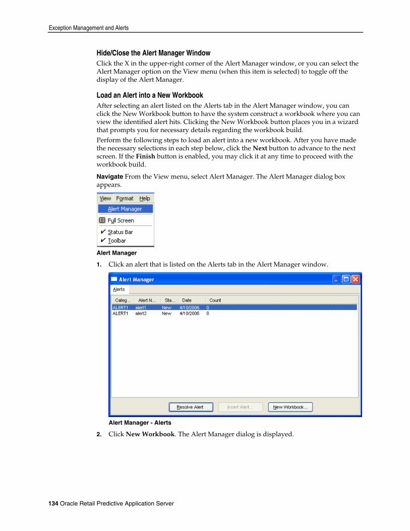
Exception Management and Alerts
134 Oracle Retail Predictive Application Server
Hide/Close the Alert Manager Window Click the X in the upper-right corner of the Alert Manager window, or you can select the Alert Manager option on the View menu (when this item is selected) to toggle off the display of the Alert Manager.
Load an Alert into a New Workbook After selecting an alert listed on the Alerts tab in the Alert Manager window, you can click the New Workbook button to have the system construct a workbook where you can view the identified alert hits. Clicking the New Workbook button places you in a wizard that prompts you for necessary details regarding the workbook build. Perform the following steps to load an alert into a new workbook. After you have made the necessary selections in each step below, click the Next button to advance to the next screen. If the Finish button is enabled, you may click it at any time to proceed with the workbook build.
Navigate From the View menu, select Alert Manager. The Alert Manager dialog box appears.
Alert Manager
1. Click an alert that is listed on the Alerts tab in the Alert Manager window.
Alert Manager - Alerts
2. Click New Workbook. The Alert Manager dialog is displayed.

Using Special RPAS Features
Using Special RPAS Features 135
Alert Manager
3. Select any additional alerts that you want to include in the new workbook, and click Next. The Alert Manager dialog is displayed.
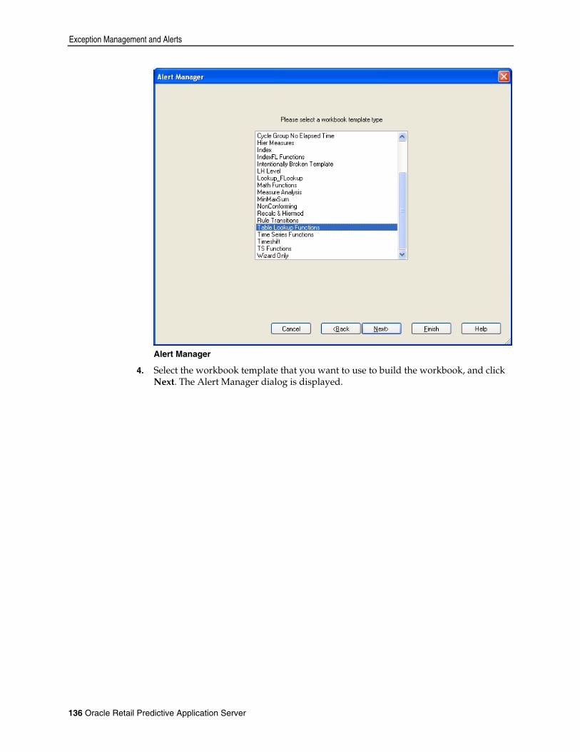
Exception Management and Alerts
136 Oracle Retail Predictive Application Server
Alert Manager
4. Select the workbook template that you want to use to build the workbook, and click Next. The Alert Manager dialog is displayed.

Using Special RPAS Features
Using Special RPAS Features 137
Alert Manager
5. Select the hierarchies that you want to range.
Note: If a hierarchy is selected to be ranged, only positions in the hierarchy that triggered an alert will be available for selection in the new workbook wizard. For instance; if you choose to range the product hierarchy, the product selection screen for the new workbook wizard will only allow you to choose product positions for which an alert was triggered. This means that all non-alert-related positions will be excluded from the workbook build.
6. Select hierarchies that you want to hide. When you select the hierarchies to hide, non-alert positions in the hierarchies you specify will not be shown in the workbook when it is initially built. If desired, these positions can later be un-hidden by accessing the Show/Hide dialog.
Note: You cannot range and hide the same hierarchy or you will get a warning message.
7. Click Next. At this time, you will be placed in the wizard for the workbook template that was selected in step 4. Follow the instructions on each wizard screen, and make selections as necessary.
8. The measure on which the loaded alert is based will be the first measure displayed in the newly-built workbook. Checkmarks identify the positions associated with a recognized alert.

Exception Management and Alerts
138 Oracle Retail Predictive Application Server
Insert an Alert into an Open Workbook You can access the Alert Manager window to insert an alert measure into a workbook that is already open. In order to view alert information, this functionality allows you to address alert-related issues without requiring you to build a new workbook. You can view multiple alert measures simultaneously in the same workbook. Whenever you insert an alert measure into an open workbook, the measure automatically becomes the active alert measure. The active alert measure for a workbook is the one that is referenced by the system when you choose menu options, such as Find Next Alert, Find Previous Alert, and Range By Alerts. Find Next Alert and Find Previous Alert will find the next or previous position in the worksheet within the active alert measure for which the alert condition is true. The Range By Alerts menu option allows you to hide all positions in a given hierarchy for which an alert condition was not triggered. This is evaluated with respect to the active alert measure. When you insert an alert measure into an open workbook, no check is made to determine whether all the positions that triggered the new alert condition are currently present in the open workbook. For example, if you chose to range hierarchies during the initial workbook build, which excludes non-alert-related positions for the original alert measure, some of the positions identified by the newly inserted alert might not be present in the open workbook. If this is the case, you will be required to build a new workbook in order to display the excluded positions. Perform the following steps to insert a new alert measure into an open workbook:
Navigate From the View menu, select Alert Manager to display the Alert Manager window. 1. Click the alert that you want to insert into the open workbook. 2. Click Insert Alert.
Change the Active Alert Measure in a Worksheet When multiple alert measures exist in a worksheet, one of the measures must be treated as the active alert measure. When you perform menu functions, such as Find Next Alert, Find Previous Alert, and Range By Alerts, the currently active alert measure is the one that the system references and uses to conduct these tasks. For example, the Find Next Alert function finds the next instance within the active alert measure where the alert condition is true (the next position where an alert has been triggered). To search for alert occurrences corresponding to a different alert measure, you must designate this measure as the active alert measure for the worksheet. To change the active alert measure, perform the following steps:
Navigate From the View menu, select Change Alert Measure. 1. Click on the measure you want to be the active alert measure. 2. Click OK. The measure that you selected is now the worksheet’s active alert measure. Whenever you select the menu options Find Next Alert or Find Previous Alert, the system will search for the next/previous position within your chosen alert measure where an alert condition has been identified. If you choose to Range By Alerts, the system evaluates your chosen active alert measure and hides all positions in a particular hierarchy that do not represent alert hits.
Resolve an Alert After taking the appropriate actions regarding identified alerts, you can use the Alert Manager window to keep track of alerts that have been resolved. Change the status of a

Using Special RPAS Features
Using Special RPAS Features 139
listed alert from New to Resolved, which indicates that appropriate actions have been taken to address the alert condition. To indicate that an alert was resolved: 1. On the Alert Manager window, click on the alert that was addressed. 2. Click Resolve Alert. The Resolved status of the alert changes to Resolved.
Note: You can reverse this action and return the alert’s Resolved status to New by selecting an alert that has already been resolved and clicking the Unresolve Alert button.
Open an Alert Workbook You can use the Alert Manager window to open an alert workbook that was already created. 1. On the Alert Manager window, click the Alert Workbooks tab. 2. Select the alert workbook that you want to open. 3. Click the Open Workbook button. The selected workbook is opened.
Resolve an Alert Workbook You can use the Alert Manager to keep track of alert workbooks that have been resolved. From the Alert Workbooks tab, you can change the status of a listed alert workbook from New to Resolved, which indicates that appropriate actions have been taken to address the alert condition.
Navigate From the View menu, select Alert Manager. 1. On the Alert Manager window, click the Alert Workbooks tab. 2. Select the alert workbook that you want to resolve.
Select alert workbook
3. Click Resolve Alert. The status of the alert changes to Resolved.

Exception Management and Alerts
140 Oracle Retail Predictive Application Server
Note: You can reverse this action and return the alert workbook’s Resolved status to Reviewed by selecting an already resolved alert workbook and clicking the Unresolve Alert button.
Alert Manager Fields Alerts are displayed as a list in the Alert window. For each alert, the following attributes are listed: Category The category to which the alert belongs. Alert Name The name of the identified alert. Priority The priority of the alert (High, Medium, or Low). Status Specifies whether the alert is resolved or unresolved. After you select an alert from
the list, you can change the status of the alert by clicking the Resolve Alert or Unresolve Alert button.
Date
The date when the Alert was identified. Count
The number of values that had this alert. Workbook
The name of the workbook that contains the alert. This field is only shown on the Alert Workbooks tab.
Alert Manager Buttons The Alert Manager window displays the following buttons: Resolve Alert Moves a new alert to the Resolved state, which identifies that you have addressed the
alert. Unresolve Alert
Moves a resolved alert to the New state, which indicates that you must readdress the alert.
Insert Alert Allows you to insert the selected alert into the open workbook. See “Insert an alert
into an open workbook” for more information. New Workbook Allows you to create a new workbook that includes the alert you selected. Clicking
the New Workbook button places you in a wizard that will prompt you for necessary details regarding the workbook. See Load an alert into a new workbook for more information.
Open Workbook Allows you to open an alert workbook that was previously created. This button is
only available on the Alert Workbooks tab.

Using Special RPAS Features
Using Special RPAS Features 141
Percent-of-Parent Measures
Overview A "percent-of-parent measure" allows you to define, view, and edit a measure as a proportion or percentage of another measure for a parent that is up one or more hierarchies. These measure relationships are also referred to as "participation measures." These measures can be viewed and edited, and they can be pre-configured in the RPAS Configuration Tools or defined in the RPAS client in a worksheet. Typical uses of this functionality are to define measures that are percentage participations of sales measures. Typically, these are: Fixed level (such as class) so the participation of each item to the class can be viewed
and manipulated To the ‘next level up’ in the product hierarchy
The following sections describe the “percent-of-parent” feature and how to create these measures in the RPAS client. The following examples will use the sample product hierarchy structure:
Sample Product Hierarchy Structure
Note: For percent-of-parent contributions in instances when very small values (with a precision of six, e.g., 0.000001) are being stored in the cell. Small values are considered to be 0.0 when determining the percent to parent contribution.
Definition and Usage Perform the following procedure to define a percent-to-parent measure. 1. Right-click the measure axis and select Create Percent of Parent Measure in the
quick menu. The Create Percent of Parent dialog appears.
Create Percent of Parent Dialog Box
2. Select the measure where a percent-of-parent measure is desired. The drop-down list contains all measures defined for the active worksheet.
3. Select the desired percent-of-parent measure type. The dialog box is context sensitive and the available parameters will change based on the type that is selected. The following sections contain detailed information about the different types and how they are defined.
Percent-of-Parent Measures
142 Oracle Retail Predictive Application Server
4. Once the type and the required parameters are assigned, click OK. The new measure appears in the worksheet.
Note: When changing the percentage of the “percent-of-parent” measure, values of the underlying measure will change to reflect the newly set percentage.
Multiple “percent-of-parent” measures can be defined for the same underlying measure; however, only one “percent-of-parent” measure or the underlying measure can be edited before calculation. All other “versions” will be protected.
The value of a “percent-of-parent” measure is a fraction that will be between zero and one. If desired, you must format the measure to be displayed as a percentage.
Absolute The “absolute” type of “percent-of-parent” measures allows you to explicitly define the parent level(s) that are used to calculate the percentage at all child levels. If you set the absolute parent level to the "class" dimension in the product hierarchy, the “percent-of-parent” measure will show: The "SKU" as a percent of the "class" at the "SKU" level The "style" as a percent of the "class" at the "style" level The "subclass" as a percent of the "class" at the "subclass" level
This is using the previously defined sample hierarchy structure. After you select the measure from the Select Measure list and select the Absolute option in the Create Percent of Parent Measure dialog box, you will see an Intersection area. This area contains drop-down lists for all hierarchies. Within these lists, the measure is dimensioned with each drop-down list, which contains the dimensions that are available for that hierarchy. 1. Select the dimension/level for each hierarchy that is to be explicitly set. 2. Click OK. A new percent-of-parent measure appears in the worksheet. For absolute
relationships, cells at or above the dimension/level will be hashed out.
Relative The "relative percent-of-parent” measure type calculates the value for a given level, which is the percentage of that level and its immediate parent (meaning one level higher). This type can only be set for a single hierarchy. Using the previously defined sample hierarchy structure, the percentages displayed are as follows: "SKU" level – The "SKU" as a percent of the "style". "style" level – The "style" as a percent of the "subclass". "subclass" level – The "subclass" as a percent of the "class".
After you select the measure from the Select Measure list and select the Relative option in the Create Percent of Parent Measure dialog box, you will see a Hierarchy drop-down list. This drop-down list contains the hierarchies on which the measure is dimensioned. 1. Select the hierarchy that will be used to calculate the percentage. Only a single
hierarchy is possible with the “relative percent-of-parent” measure type. 2. Click OK. The new percent-of-parent measure appears in the worksheet.

Using Special RPAS Features
Using Special RPAS Features 143
Certain dimensions will have multiple parents if there are multiple branching hierarchies. For relative percent-of-parent measures, the calculation of the percentage is always based on the active roll-up in the current window. The calculated value is based on the actual next level up in the hierarchy, which is based on the hierarchy structure (not necessarily the one that is displayed). In the previous examples, imagine that SKU-subclass-class is displayed in the client, but the underlying structure is SKU-style-subclass-class. When viewing the value at SKU; the percentage is based on style (not the subclass even though style is not displayed). Cells at the top of the hierarchy are hashed out because those values cannot be calculated.


Appendix: Using RPAS Menus and Toolbars 145
A Appendix: Using RPAS Menus and Toolbars
Application Main Menu Bar The menu bar and the items contained in each menu are context-sensitive, and they change according to what you are working on and how you are working. Menu items that are grayed out are not available to you in your current work mode. When no workbooks are open, the menu bar displays the following options:
When a workbook is open, the menu bar displays the following options:
Menu Shortcuts You can also access menus by pressing the Alt key followed by the underlined letter for the menu item. For example, <Alt+F> accesses the File menu. Some menu items have shortcut key combinations, which have the key combination displayed next to the menu item name. For example, Ctrl+N accesses the New file dialog box. In addition to key combinations, some menu items can be directly accessed from toolbar buttons.
File Menu The File menu contains the following options:
File – Change Password See Chapter 3.
File – New See Chapter 3.
File – Open See Chapter 3.
File – Save Select File – Save to store all of the information in the workbook, which includes the current layout of the worksheets and charts. If the workbook you are working on has been saved, selecting this menu item will update the stored information. If the workbook has not been saved, selection of this menu item will open the Save As dialog box, which prompts you for a workbook name. The Save menu item is only enabled when a workbook has been created or opened. Saving a workbook does not commit it to the master database. You must select Commit Now or Commit Later from the File menu to commit your changes to the master.
File Menu
146 Oracle Retail Predictive Application Server
File – Save As The Save As menu option opens a dialog box where you can specify the name of the workbook to be saved. You can also specify the nature of access privileges associated with the workbook. The default access privilege is the creator of the workbook alone, but you can also grant group access privileges or world access privileges. The Save As menu option is only enabled when a workbook is open. Type a name for the workbook in the Workbooks text field of the Save As dialog. Use the following Save Access As radio buttons to specify access privileges for this workbook: User – only you can access and make changes to the workbook. Group – only those users who are in your group (as determined by your System
Administrator) can edit the workbook. World – any user can update the workbook.
All of the workbooks that were previously saved are listed when the Save As dialog box is displayed. When viewing the list of previously saved workbooks, click on any column header to sort the workbooks by that attribute. For example, click the Owner header to sort the workbooks alphabetically by owner. If you select the List all workbooks check box, all workbooks in the system (including those to which you do not have write access) will be displayed. Keep in mind that listing those additional workbooks does not give you write access to them. Click OK to save the workbook, or click Cancel to return to the workbook without saving.
File – Close The Close menu option is only available when a workbook is open. If the workbook was previously saved and no new changes have been made, selecting Close will close the workbook. If the current workbook has not been saved, or if changes were made since the last save, selecting this item will display the Close dialog box with the following choices: Save – If the workbook was previously saved, selecting Save will save the workbook
with the current name and then close it. If the workbook was not previously saved, Save will display the Save As dialog box where you specify the name of the workbook before closing it.
Commit Now – This commits the changes to the master database and closes the workbook. If it is not necessary to immediately commit the workbook to the master database, use the Commit Later option.
Commit Later – This places the workbook name in a list of workbooks that will be committed to the master database at a later time during a batch process. Whenever possible, use Commit Later instead of Commit Now to maximize productivity.
Save and Commit Now – This performs both of the functions described above. If the workbook was previously saved, the system: Saves the workbook under its current name Commits the new changes to the master database Closes the workbook
File Menu
Appendix: Using RPAS Menus and Toolbars 147
If the workbook was not previously saved, the Save As dialog box is displayed, and it will prompt you for a workbook name. The workbook is saved under this name, the changes are committed to the master database, and the workbook is closed. Save and Commit Later – This performs both of the functions described above. If the
workbook was previously saved, the system saves the workbook under its current name. It then places that name on a list of workbooks to be committed in a batch process at a later time, and it closes the workbook. If the workbook was not previously saved, the Save As dialog box is displayed, and it prompts you for a workbook name. The workbook is saved under this name, the “Commit Later” function is executed, and the workbook is closed.
Ignore Changes – This closes the workbook without saving or committing any changes.
Cancel – This returns you to the open workbook.
File – Delete See Chapter 3.
File – Exit See Chapter 3.
File – Logoff See Chapter 3.
File – Commit Status See Chapter 3.
File – Commit ASAP See Chapter 3.
File – Export Sheet The Export Sheet menu option exports the current view for the worksheet to an output file on the client machine. Selection of this item displays a Save As dialog box where you can specify: The output file name The directory where the file will be saved Other customizable options
In the Save As dialog, use the Save In list to select the directory where you want the file to be exported. When the appropriate directory is selected, enter an output file name in the File Name field, or select one from the list of those displayed. If you do not enter or select an output file name, a file extension is automatically attached to the name you select. The Save As Type list allows you to select the format of the output file that you create. When you type in the file name you want at the top of the dialog box, the appropriate file extension is attached to that name as determined by your selection in the Save As list. Typical Save As file types are: .TXT – Text file .DIF – Data interchange format
File Menu
148 Oracle Retail Predictive Application Server
The Delimiter option allows you to specify the character that is used to separate information in the output file. Standard choices for this character are Tab, Comma, or Space; but you can specify any character you want by selecting the Other radio button. This option is available only for text file exports. The Labels option specifies the format of the label headers across the top of every cell in the output file. The choices for the Labels option include: Do Not Include – Labels are not provided at the top of data cells. Include Once – Only one label is placed across the top of each section of cells. Repeat: Labels – Repeated as necessary across the top of every data cell.
The Description option allows you to determine whether labels or names are used when specifying certain positions in your exported file. For example, the position name for a store in the RDF system might be STR_4540 and the label for that position name might be 52-4540 GA/Atlanta. The names are more concise, but the full labels are more descriptive and informative. The choices for the Description option are: Labels – Uses the full, descriptive label assigned to a position. Names – Uses the concise, actual position name in the system.
When you have named your output file and made the appropriate selections, click OK to export the file, or click Cancel to return to the workbook without exporting.
File – MRU (Most Recently Used) List The MRU (Most Recently Used) list is located directly beneath the Exit option on the File menu. The MRU list is a list of the four most recently opened workbooks. When a workbook is displayed on the MRU list, it can be quickly accessed by selecting that workbook directly from the File menu. If you open a workbook that already exists, and you save it under a new name by selecting Save As from the File menu, the old and the new workbook names will appear on the MRU list.
File – Page Setup The Page Setup dialog box contains options for the format of the print output of a document. This option always overrides the settings that were established in the Windows Print Setup dialog box, and the settings only apply to the current document (worksheet or chart). There are five options available in this dialog box, which are presented in a tab format: Page – Allows you to specify the page orientation (portrait vs. landscape) and
customize (scale) the size of the printed output. Margins – Allows you to specify and preview the page margins (expressed in
inches). Header/Footer – Allows you to customize the header and footer information that
appears on the pages of your output. You may select information to be displayed on the left, center, and right portions of your header and footer.
Sheet – Allows you to select how you want row and column label information displayed, and specify the appearance of horizontal and vertical grid lines. This tab also allows you to set the order of page numbering (left to right, top to bottom).
Page Breaks – Allows you to specify the placement of page breaks for printed output.
When you have made your selections, click OK to apply the changes to the page setup. Click Cancel to return to the worksheet without making changes to the page setup. The
File Menu
Appendix: Using RPAS Menus and Toolbars 149
Apply button is only functional when Page Setup is used in conjunction with the Print Preview screen. Click the Apply button to view your selections in Print Preview mode without closing the “Page Setup” dialog.
File – Print The Print menu option displays the Print dialog box where you select printing options such as printer, print range, and number of copies. Printer – Click the drop-down list in this dialog section to specify the path and name
of the printer that you want to use. Print Range – Click the appropriate radio button to designate the range for the
printed output. All – Prints every page in the workbook. The ordering of page numbers (top to
bottom or left to right) can be specified on the Sheet tab of the Page Setup dialog. Pages – Allows you to specify a subset of pages to be printed. In the fields provided,
enter the numbers of the first and last pages in the range to be printed.
Usability Tip: Use the Print Preview option on the File menu to determine the page numbers of the information you want to print. It may be helpful to use the custom header/footer feature in Page Setup to insert page number field marker codes in your document.
Slice – Allows you to specify a range of complete slices to be printed. The slice axis runs perpendicular to the plane of the computer screen. A separate slice exists for each element of the dimension represented by the hierarchy tile that resides in the slice display area. In the boxes provided, enter the numbers of the first and last slice in the range to be printed.
Copies – Enter the number of copies to be printed, or use the spin buttons to increment the copy total.
File – Print Multiple The Print Multiple menu option produces a dialog that allows you to select multiple worksheets to submit to the print queue. Use Crtl+Click to select multiple worksheets from the list. Select the Display print dialog before each window option to have the Print Options dialog displayed individually before each worksheet is printed. Click OK to submit your selections to the print queue. The standard Print Options dialog is presented to allow you to make print option selections. Selections made on this dialog will apply to all printed worksheets if the Display print dialog before each window is not selected. If the box was checked, this dialog will reappear before each worksheet is printed.
File – Print Preview The Print Preview option displays a standard print preview window, so you can view the output before printing. Click the Previous Page or Next Page button to page backward and forward through
the document. This can also be done by using the standard vertical scroll bar. Click the Zoom In or Zoom Out button to change the magnification of your
document.
Edit Menu
150 Oracle Retail Predictive Application Server
Click the Page Setup button to access the Page Setup dialog. Here you can modify document features such as page orientation, scaling, margins, headers/footers, page numbering scheme, and page breaks.
Click the Close button to close the Print Preview dialog and return to the main document view.
File – Refresh The selective/partial Refresh feature allows you to refresh a portion of your workbook measures with original domain data while leaving other measures unchanged.
Edit Menu The Edit menu contains the following options:
Edit – Cut The Cut menu option copies selected worksheet data to an application clipboard and clears the data from the worksheet cells. Select the data cells whose contents are to be cut, and then select Cut from the Edit menu. Only data from writable measures can be cut. When you use the Edit – Cut option to cut data, the function performs the cut at the current hierarchical level. Data can be cut from only one dimensional level at a time, so if multiple dimensions are represented in your grid selections, the cut is performed at the lowest dimensional level actually selected. If data cells are selected in the grid before you invoke the Edit – Cut option, only data from those selected cells will be cut. Note that the Cut operation treats the currently displayed position on the slice axis as the only selected slice position.
Note: The Cut command does not copy information to your Windows clipboard. The data is copied to an application-specific clipboard and cannot be pasted into other programs. If you intend to paste the data into another application, you can choose the Edit – Copy to Clipboard command.
Edit – Cut Special The Cut Special option copies selected worksheet data to an application clipboard and clears the data from the copied cells. Unlike the Edit – Cut operation, the Cut Special command provides a dialog where you can specify options for specialized cut functions, including cutting data at base level and cutting data from all worksheet slices. Select the data cells whose contents are to be cut, and then select Cut Special from the Edit menu. Only data from writable measures can be cut.

Edit Menu
Appendix: Using RPAS Menus and Toolbars 151
Cut Special Dialog
Note: The Cut command does not copy information to your Windows clipboard. The data is copied to an application-specific clipboard, and it cannot be pasted into other programs. If you intend to paste the data into another application, you can choose the Edit – Copy to Clipboard command.
Cut Data at Base Level The Cut Data at Base Level option allows you to cut data at an applicable dimensional level beneath the level selected in the grid. This feature allows you to view data at an aggregate level while cutting data at a dimensional level that is not currently displayed. When you select the Cut Special function at an aggregate level and you select the Cut Data at Base Level check box, all base level data applicable to that selected aggregate data will be cut and copied to the application clipboard. Although the cut function is actually performed at the base dimensional level, it seems that the aggregate level data has been cut (due to the process of data rollup).
Cut All Slices When you make cell selections prior to cutting data, the system only allows for the selection of the currently displayed position along the slice axis. The Cut Special dialog; however, contains a check box that allows you to specify that data should be cut for all positions (pages) in this axis. When the box is checked, the cut operation behaves as if all positions in the slice dimensions were selected prior to the cut. If the box is left unchecked, only data from the currently displayed slice position will be cut.
Cutting Data While in Outline View Outline View allows you to view data for multiple dimensional levels simultaneously in the same worksheet. The system; however, allows the cutting of data from only one dimensional level at a time. Whenever multiple dimensions are displayed in outline view for a given hierarchy, the Cut Special dialog requires you to select the dimensional level at which you want to cut data. The Cut Special dialog has drop-down lists that are enabled for each hierarchy displayed in outline mode.

Edit Menu
152 Oracle Retail Predictive Application Server
Edit – Copy The Copy menu option copies selected worksheet data to an application clipboard. Edit – Copy is typically used with the Edit – Paste command to speed the process of populating data cells in a worksheet. Select the data cells whose contents are to be copied, and then select Copy from the Edit menu. When you use the Edit – Copy option to copy data, the function performs the copy at the current hierarchical level. Data can only be copied from one dimensional level at a time, so if multiple dimensions are represented in your grid selections, the copy is performed at the lowest dimensional level actually selected. Unlike the Cut function, Copy does not clear the data from the copied cells. If data cells are selected in the grid before you invoke the Edit – Copy command, only data from those selected cells will be copied. Note that the Copy operation treats the currently displayed position on the slice axis as the only selected slice position. If there are no data cells selected in the grid at the time the Copy function is invoked, the system will copy the data for every cell in the worksheet.
Note: The Copy option does not copy information to your Windows clipboard. The data is copied to an application-specific clipboard, and it cannot be pasted into other programs. If you intend to paste the data into another application, you can choose the Edit – Copy to Clipboard command.
Edit – Copy Special The Copy Special menu option copies selected worksheet data to an application clipboard. Unlike the Edit – Copy operation, the Copy Special command provides a dialog where you can specify options for specialized copy functions. This includes copying data at base level and copying data from all worksheet slices. Select the data cells whose contents are to be copied, and then select Copy Special from the Edit menu.
Copy Special Dialog
Note: The Copy Special command does not copy information to your Windows clipboard. The data is copied to an application-specific clipboard and cannot be pasted into other programs. If you intend to paste the data into another application, you can choose the Edit – Copy to Clipboard command.
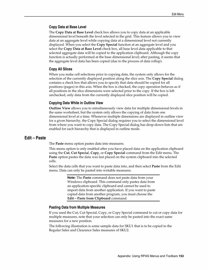
Edit Menu
Appendix: Using RPAS Menus and Toolbars 153
Copy Data at Base Level The Copy Data at Base Level check box allows you to copy data at an applicable dimensional level beneath the level selected in the grid. This feature allows you to view data at an aggregate level while copying data at a dimensional level not currently displayed. When you select the Copy Special function at an aggregate level and you select the Copy Data at Base Level check box, all base level data applicable to that selected aggregate data will be copied to the application clipboard. Although the copy function is actually performed at the base dimensional level; after pasting, it seems that the aggregate level data has been copied (due to the process of data rollup).
Copy All Slices When you make cell selections prior to copying data, the system only allows for the selection of the currently displayed position along the slice axis. The Copy Special dialog contains a check box that allows you to specify that data should be copied for all positions (pages) in this axis. When the box is checked, the copy operation behaves as if all positions in the slice dimensions were selected prior to the copy. If the box is left unchecked, only data from the currently displayed slice position will be copied.
Copying Data While in Outline View Outline View allows you to simultaneously view data for multiple dimensional levels in the same worksheet, but the system only allows the copying of data from one dimensional level at a time. Whenever multiple dimensions are displayed in outline view for a given hierarchy, the Copy Special dialog requires you to select the dimensional level from where you want to copy data. The Copy Special dialog has drop-down lists that are enabled for each hierarchy that is displayed in outline mode.
Edit – Paste The Paste menu option pastes data into measures. This menu option is only enabled after you have placed data on the application clipboard using the Cut, Cut Special, Copy, or Copy Special command from the Edit menu. The Paste option pastes the data was last placed on the system clipboard into the selected cells. Select the data cells that you want to paste data into, and then select Paste from the Edit menu. Data can only be pasted into writable measures.
Note: The Paste command does not paste data from your Windows clipboard. This command only pastes data from an application-specific clipboard and cannot be used to import data from another application. If you want to paste copied data from another program, you must choose the Edit – Paste from Clipboard command.
Pasting Data from Multiple Measures If you used the Cut, Cut Special, Copy, or Copy Special command to cut or copy data for multiple measures, note that your selection can only be pasted into the exact same measures for a new position. The following illustration is some sample data for SKU1 that is to be copied to the Regular Sales and Clearance Sales measures of SKU2.
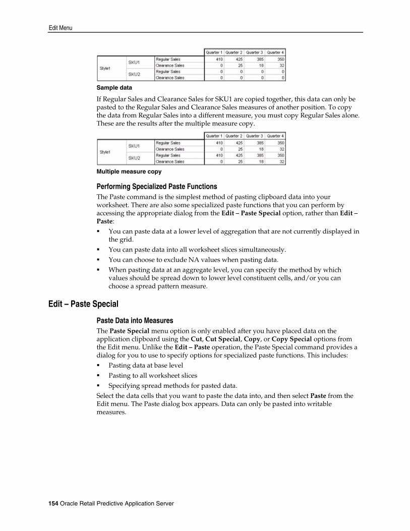
Edit Menu
154 Oracle Retail Predictive Application Server
Sample data
If Regular Sales and Clearance Sales for SKU1 are copied together, this data can only be pasted to the Regular Sales and Clearance Sales measures of another position. To copy the data from Regular Sales into a different measure, you must copy Regular Sales alone. These are the results after the multiple measure copy.
Multiple measure copy
Performing Specialized Paste Functions The Paste command is the simplest method of pasting clipboard data into your worksheet. There are also some specialized paste functions that you can perform by accessing the appropriate dialog from the Edit – Paste Special option, rather than Edit – Paste: You can paste data at a lower level of aggregation that are not currently displayed in
the grid. You can paste data into all worksheet slices simultaneously. You can choose to exclude NA values when pasting data. When pasting data at an aggregate level, you can specify the method by which
values should be spread down to lower level constituent cells, and/or you can choose a spread pattern measure.
Edit – Paste Special
Paste Data into Measures The Paste Special menu option is only enabled after you have placed data on the application clipboard using the Cut, Cut Special, Copy, or Copy Special options from the Edit menu. Unlike the Edit – Paste operation, the Paste Special command provides a dialog for you to use to specify options for specialized paste functions. This includes: Pasting data at base level Pasting to all worksheet slices Specifying spread methods for pasted data.
Select the data cells that you want to paste the data into, and then select Paste from the Edit menu. The Paste dialog box appears. Data can only be pasted into writable measures.
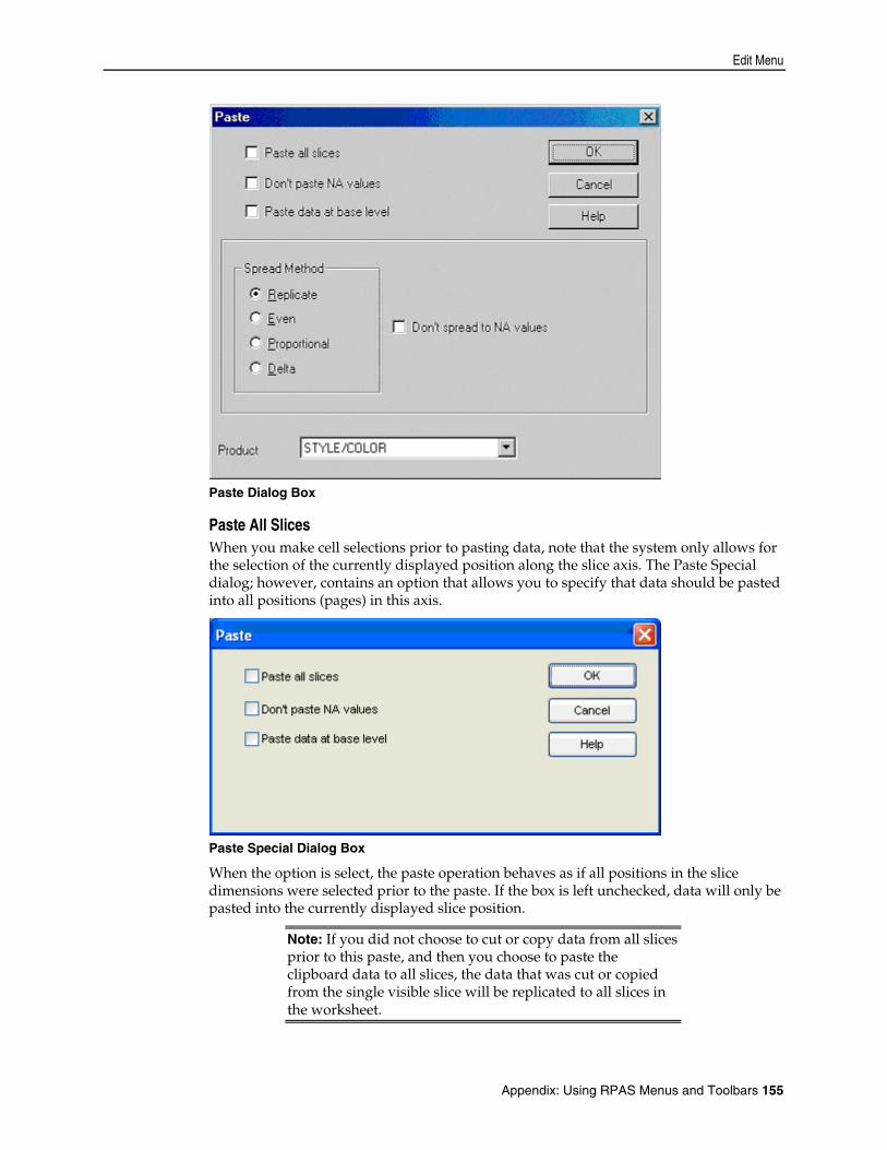
Edit Menu
Appendix: Using RPAS Menus and Toolbars 155
Paste Dialog Box
Paste All Slices When you make cell selections prior to pasting data, note that the system only allows for the selection of the currently displayed position along the slice axis. The Paste Special dialog; however, contains an option that allows you to specify that data should be pasted into all positions (pages) in this axis.
Paste Special Dialog Box
When the option is select, the paste operation behaves as if all positions in the slice dimensions were selected prior to the paste. If the box is left unchecked, data will only be pasted into the currently displayed slice position.
Note: If you did not choose to cut or copy data from all slices prior to this paste, and then you choose to paste the clipboard data to all slices, the data that was cut or copied from the single visible slice will be replicated to all slices in the worksheet.

Edit Menu
156 Oracle Retail Predictive Application Server
Don't Paste NA Values If the Don't Paste NA Values option is selected, the system will not paste cut or copied NA data values into the current selection. Whenever the system encounters an NA value in the clipboard data, that value is ignored and the data cell being pasted keeps its original value. In other words, when this option is selected, current grid data is not overwritten by NA values.
Paste Data at Base Level The Paste Data At Base Level check box allows you to paste data at an applicable dimensional level beneath the one selected in the grid. This feature allows you to view data at an aggregate level while pasting data at a dimensional level that is not currently displayed. When you select the Paste function at an aggregate level and you select the Paste Data At Base Level check box, all base level data applicable to that selected aggregate data will be pasted into the selected data cells.
Note: Whenever data has just been cut or copied at a base level, the Paste Data At Base Level check box defaults to Selected.
Specifying Spread Method for Pasted Data The bottom portion of the Paste dialog is enabled when you are pasting data at a level other than base. The options in this section control how data pasted into an aggregate level is spread down to lower dimensional levels. If the Paste Data at Base Level option is selected, this portion of the dialog becomes disabled. The Spread Method radio buttons allow you to specify the way that aggregate cell data is to be spread to lower dimensions: Replicate – Any value pasted in an aggregate level cell will be replicated exactly to
every base level cell that comprises the aggregate total.
Note: After the spread, this method results in a recalculation of the aggregate cell totals.
Even – Any value pasted into an aggregate level cell will be spread evenly among that cell's lower level constituents.
Proportional – Any value pasted in an aggregate level cell will be spread proportionally among all lower level constituent cells. This is based on these cells' contents before the paste.
Delta – The difference between the value pasted in the aggregated cell level and the original value of the aggregate cell level will be spread evenly among all lower-level constituent cells.
When the Don’t Spread to NA Values option is selected, pasted aggregate data is not spread to lower level cells that contain NA values before the paste. The NA values are left intact, and the aggregate data is spread to the remaining lower level cells that comprise the aggregate total.
Pasting Data While in Outline View Outline View allows you to simultaneously view data for multiple dimensional levels in the same worksheet, but the system only allows the pasting of data into one dimensional level at a time. Whenever multiple dimensions are displayed in outline view for a given hierarchy, the Paste Special dialog requires you to select the dimensional level at which

Edit Menu
Appendix: Using RPAS Menus and Toolbars 157
you want to paste data. The Paste Special dialog has drop-down lists that are enabled for each hierarchy displayed in outline mode.
Pasting from One Position to Many Positions Multi-cell cut and copy regions that contain a single position in a dimension can be pasted into a larger region that contains more positions along that same dimension. In such cases, the entire cut and copy region is replicated across the additional positions in the paste region. For example, it is possible to copy data from a single store but for multiple weeks, and then paste that data into multiple stores. The copy region would simply be replicated for each new store in the paste selection. The following figures provide an example of the one-to-many paste functionality. Data from four weeks at a single store position is copied (the copy region is shaded in the first figure), and this data is pasted to the other four locations.
Single store position
Multiple locations
Edit – Paste from Clipboard The Paste from Clipboard option pastes data from the Windows clipboard into selected worksheet cells. Use this paste operation if you want to paste data from another application into the current worksheet. Select the data cells where you want to paste clipboard data, and then select Paste from Clipboard from the Edit menu.
Note: When using this command, the maximum number of cells that can be pasted is limited by memory. This operation should not be used to import data for entire workbooks.
Edit – Revert The Revert menu option reverts to the most recently saved version of the workbook. This option allows you to return to a prior state without having to close the workbook, select Ignore Changes from the Close dialog box, and reopen the workbook. The Revert option is only enabled if the current workbook has already been saved under a specified name, and if changes have been made to the data since the last save. When you select Revert from the Edit menu, the Revert dialog box opens to inform you that all changes made since the last save will be lost.
Edit Menu
158 Oracle Retail Predictive Application Server
Click OK to abandon the current workbook and return to the most recently saved version, or click Cancel to keep the changes you have made and return to the current workbook.
Edit – Fill The Fill menu option quickly populates the cells in a worksheet. This command fills only one measure at a time. If there are no data cells selected in the grid at the time the Fill dialog box is opened, the system will fill the data cells for the entire measure that you select in the Measure drop-down list. If certain data cells were selected in the grid, only those selected data cells will be filled. Select the measure to be filled from the Measure drop-down list. This field only displays writable measures. The properties of the Fill Value field change depending on your selection in the Measure drop-down list. If the selected measure contains values restricted to a list, the Fill Value field will change to a drop-down list in which you can select the appropriate value. If the measure selected is numeric or alphanumeric, the Fill Value field allows you to enter the value that you want entered in the effected cells.
Specifying Spread Method for Filled Data The lower portion of the Fill dialog is enabled when you are filling data into worksheet cells at an aggregate level. This section allows you to specify the method by which aggregate data is to be spread to lower level constituent cells. The Spread Method radio buttons allow you to specify the way that aggregate cell data is to be spread to lower dimensions. The options are: Replicate – Any value filled into an aggregate level cell will be replicated exactly to
every base level cell that comprises the aggregate total.
Note: After the spread, this method results in a recalculation of the aggregate cell totals.
Even – Any value filled into an aggregate level cell will be spread evenly among that cell's lower level constituents.
Proportional – Any value filled into an aggregate level cell will be spread proportionally among all lower level constituent cells. This is based on these cells' contents before the fill.
Delta – The difference between the value pasted in the aggregated cell level and the original value of the aggregate cell level will be spread evenly among all lower-level constituent cells.
When the Don’t Spread to NA Values check box is selected, filled aggregate data is not spread to lower level cells that contain NA values before the fill. The NA values are left intact, and the aggregate data is spread to the remaining lower level cells that comprise the aggregate total.
Filling Data while in Outline View Outline View menu option allows you to simultaneously view data for multiple dimensional levels in the same worksheet, but the system only allows the filling of data into one dimensional level at a time. Whenever multiple dimensions are displayed in outline view for a given hierarchy, the Fill dialog requires you to select the dimensional level where you want to fill data. The Fill dialog has drop-down lists enabled for each hierarchy displayed in outline mode.

Edit Menu
Appendix: Using RPAS Menus and Toolbars 159
Edit – Clear Contents The Clear Contents menu option quickly clears the contents of the cells in a worksheet. Select the data cells that you want to clear, and choose Clear Contents from the Edit menu. If there are no data cells selected in the grid at the time the Clear Contents function is invoked, the system will attempt to clear the data for every cell. However, if your grid data contains any measures that are read-only, the system will be unable to clear data for the entire worksheet. In this case, a message informs you that the system could not complete the request.
Edit – Find The Find menu option locates a specified position in any axis. This function allows you to perform an alphanumeric search for text entered in the Find What field of the dialog. This function can be useful in various circumstances (for example, when you want to move quickly to a particular SKU item in a very large worksheet). In the Find dialog, the Look In drop-down list allows you to narrow your search to one of the three available axes: Row Axis, Column Axis, or Slice Axis. The Match Case and Find Exact Match Only options allow you to further narrow your search by imposing more restrictions. Click Find Next to search for the next matching occurrence.
Edit – Insert Measure The Insert Measure menu option displays a dialog that allows you to select a measure or group of measures to be inserted in a currently open workbook. This functionality reduces the need to build new workbooks whenever a view of currently unrepresented measures is required. The ability to insert new measures into open workbooks is particularly useful in the context of establishing access to alerts. A worksheet must be open and active for the Insert Measure menu option to be enabled. Any measure(s) selected to be inserted in the workbook will be placed on the currently active worksheet. The Insert Measure dialog box allows for an intelligent selection of measures based on your specifications of the four components (role, version, units, and metric) of a registered measure. Make selections for these four components by clicking on the desired items in the Role, Version, Units, and Metric lists. You can select multiple items in a list by using <Ctrl + Click>. Any measures that are constructed using some combination of component selections will appear in the Measures list. From this list, select the final measure(s) that you want to insert, and click OK.
Insert a Measure into an Open Worksheet If you have the necessary access rights, you can insert a new measure or group of measures into an open workbook. This functionality reduces the need to build new workbooks whenever a view of currently unrepresented measures is required. The ability to insert new measures into open workbooks is particularly useful when establishing access to alerts. Use the following procedure to select a measure or group of measures to be inserted in a currently open workbook.

Edit Menu
160 Oracle Retail Predictive Application Server
Note: A worksheet must be open and active for the Insert Measure menu option to be enabled. Any measure(s) selected to be inserted in the workbook will be placed on the currently active worksheet.
Navigate From the Edit menu, select Insert Measure. 1. Select the desired measure(s) in the Measures list. 2. Click OK.
Edit – Automatic Calculation The Automatic Calculation menu option places the system in automatic calculation mode. In this mode, every change to a cell in the spreadsheet causes a recalculation, which requires immediate communication from the worksheet (client) back to the database (server). In this mode, there may be an appreciable pause between making a change and being able to effect the next change. A check mark is displayed beside either the Automatic Calculation option or the Manual Calculation option to indicate the mode the system is currently in. Select the desired menu option to change calculation modes.
Edit – Manual Calculation The Manual Calculation menu option places the system in deferred (manual) calculation mode. In this mode, worksheet changes are collected until you manually submit the queue to the server for processing. Changes made to data cells are shown in italic font until they are sent to the server. A check mark is displayed beside either the Automatic Calculation option or the Manual Calculation option to indicate the mode the system is currently in. Select the desired menu option to change calculation modes.
Edit – Calculate Now The Calculate Now menu option submits a queue of data changes to the server for processing. Queued changes are executed in the order that they were made. This menu option is only enabled when the system is in manual (deferred) calculation mode.
Edit – Remove Last Deferred Entry The Remove Last Deferred Entry menu option removes the last deferred data entry from the list of queued items to be sent to the server for processing. This option allows you to undo the last data change made and return the contents of the affected cell to its original value. This menu option is only enabled when the system is in manual (deferred) calculation mode.
Edit – Remove All Deferred Entries The Remove All Deferred Entries menu option removes all pending deferred data changes from the list of queued items to be sent to the server for processing. This option allows you to undo all data changes made since the last set of deferred entries was processed. When this option is selected, the original contents of the affected

View Menu
Appendix: Using RPAS Menus and Toolbars 161
cells are restored. This menu option is only enabled when the system is in manual (deferred) calculation mode.
View Menu The View menu contains the following options:
View – Grid This option switches to the grid view of your worksheet when you are in Chart view. You may also use Toggle to switch between the chart and the grid.
Toggle toolbar button
View – Chart This option switches to the chart view of your worksheet when you are in Grid view. All numeric data or subsets of such data in a worksheet can be easily converted to a graphical chart. You can also use Toggle to switch between the chart and the grid.
Toggle toolbar button
In the Chart view, the grid rows are displayed on the y-axis, the grid columns are displayed on the x-axis, and the current visible slice position is displayed on the z-axis. If there are items selected in the grid at the time the view is toggled to Chart, the chart will only display those items. If there is no selection, the chart will display all items (for a maximum of 1000 positions). The Chart view is created at the current aggregate level of the grid.
View – Alert Manager See Chapter 3.
View – Full Screen See Chapter 3.
View – Zoom The Zoom menu option displays the Zoom dialog. This dialog allows you to enlarge the grid contents of the active window for easier viewing, or reduce the size of the contents in order to fit as much data on the terminal display as possible. A different zoom level can be specified for each worksheet in a workbook. When a workbook is closed, the current zoom level for each worksheet is saved. The grid view zoom level only affects the display of data on the computer terminal. Zooming does not affect the scaling value set in Page Setup and has no effect on printing.
View – Status Bar See Chapter 3.
Format Menu
162 Oracle Retail Predictive Application Server
View – Toolbar See Chapter 3.
View – Find Previous Alert The Find Previous Alert menu option scrolls the worksheet to the previous occurrence of an alert. When searching for the previous alert, the system begins in the current alert cell and scans the active alert measure backward by rows. When an alert is found, the worksheet is scrolled so that the cell containing the alert appears in the worksheet window.
View – Change Alert Measure The Change Alert Measure menu option produces a dialog from which you choose the active alert measure for the worksheet. When more than one alert measure exists in a worksheet, one must be the active alert referenced when performing such menu commands as Find Next Alert and Find Previous Alert.
View – Next in Flow Control The Next in Flow Control provides a menu-driven method of advancing to the next step in the business process. Each distinct step is associated with a separate worksheet or a set of worksheets. Choosing this option has the same effect as clicking the Next toolbar button. The steps in the business process are represented by the flow control tabs, which normally appear immediately beneath the application toolbar. To view the worksheet(s) associated with a particular step, you can click the corresponding tab.
View – Previous in Flow Control The Previous in Flow Control menu options provide a menu-driven method of returning to the previous step in the business process. Each distinct step is associated with a separate worksheet or set of worksheets. Choosing this option has the same effect as clicking the Previous toolbar button. The steps in the business process are represented by the flow control tabs, which normally appear immediately beneath the application toolbar. To view the worksheet(s) associated with a particular step, you can click on the corresponding tab.
View – Sort The Sort menu option displays the Create Sort Attribute dialog box. This dialog allows you to create a user-named attribute based on selected grid data that can be used to sort and re-sort data in the attribute’s corresponding dimension. The sorting mechanism allows you to sort one dimension in a hierarchy according to current data values in the grid. To sort data, you must first select a one-dimensional data space (a single column or row of data in the grid). Once the data is selected, choose the View – Sort menu option to display the Create Sort Attribute dialog box.
Format Menu The View menu contains the following options:
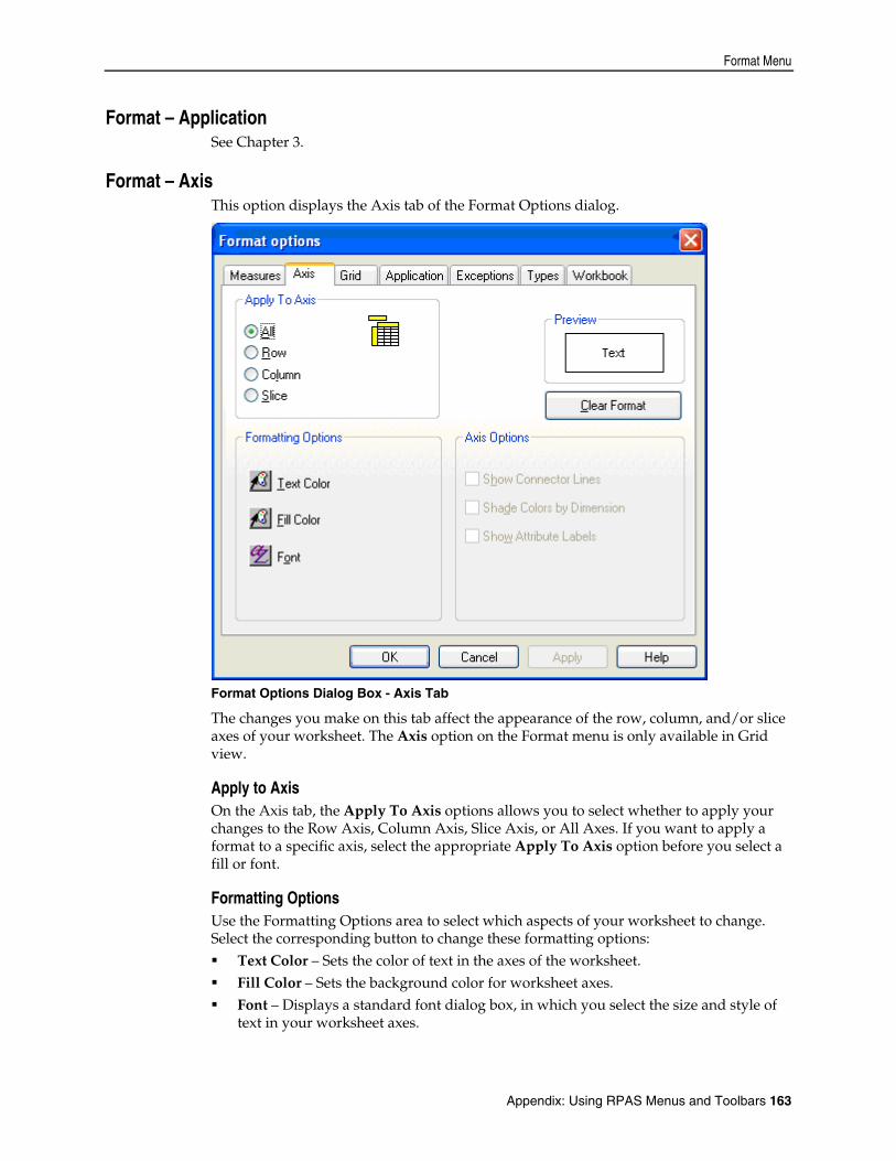
Format Menu
Appendix: Using RPAS Menus and Toolbars 163
Format – Application See Chapter 3.
Format – Axis This option displays the Axis tab of the Format Options dialog.
Format Options Dialog Box - Axis Tab
The changes you make on this tab affect the appearance of the row, column, and/or slice axes of your worksheet. The Axis option on the Format menu is only available in Grid view.
Apply to Axis On the Axis tab, the Apply To Axis options allows you to select whether to apply your changes to the Row Axis, Column Axis, Slice Axis, or All Axes. If you want to apply a format to a specific axis, select the appropriate Apply To Axis option before you select a fill or font.
Formatting Options Use the Formatting Options area to select which aspects of your worksheet to change. Select the corresponding button to change these formatting options: Text Color – Sets the color of text in the axes of the worksheet. Fill Color – Sets the background color for worksheet axes. Font – Displays a standard font dialog box, in which you select the size and style of
text in your worksheet axes.

Format Menu
164 Oracle Retail Predictive Application Server
Axis Options The available options affect the axis display of axes that are currently in outline view. Axis options can only be changed for one grid axis at a time. Click the check boxes to toggle the display of the following axis options: Show Connector Lines – Toggles the display of connector lines in the selected axis
when multiple dimensions are displayed in outline view. Shade Colors by Dimension – Toggles the use of a shading scheme to differentiate
dimensions in the axis and grid display. When this check box is selected, position labels and data cells that belong to different hierarchical levels are shaded differently.
Show Attribute Labels – Toggles the display of label headers that designate attributes for positions appearing along the chosen axis. For the column axis, these attribute labels appear to the left of the column axis header area. For the row axis, the labels appear directly above the row axis header area.
Note: This option turns on/off the display of attribute labels. To turn on the display of position attribute values, right-click over the desired axis and choose Select Display and Sort Attributes from the menu.
Preview Window The Preview window provides a sample view of your changes.
Clear Format The Clear Format button removes all formatting options from the selected axis. Click Apply to make your changes without closing the dialog box. Click OK to make the changes and return to your worksheet. Click Cancel to close the dialog box without applying any format changes.
Note: Cancel does not undo any changes that have already been made using the Apply button.
Format – Chart The Chart menu option on the Format menu is only available when you are viewing data in Chart mode. This menu item allows you to customize a variety of chart features; including chart type, color scheme, title style, axis settings, and 2D/3D aspects. Select Format-Chart or click the Format button on the workbook toolbar. The Chart F/X Properties dialog box appears.

Format Menu
Appendix: Using RPAS Menus and Toolbars 165
Chart FX Properties Dialog Box - General Tab
Format – Chart – 3D The 3D tab of the Chart FX Properties dialog allows you to customize properties of three-dimensional charts. The features on the 3D tab are only enabled when your chart is displayed in 3D view. To change your chart to 3D mode, select the 3D option on the General tab in Chart FX Properties dialog box, which is accessed by selecting Format – Chart.
Rotated View The Rotated View option allows you to toggle between the standard three-dimensional view of your chart and your customized, rotated view. Select this check box to convert your chart to the rotated view specified by selections made on the 3D dialog. This field is only enabled when you are viewing your chart in 3D mode.
X Angle If Rotated View is selected, the X Angle field allows you to enter the numeric value of the x-axis rotation angle. The rotation of the x-axis can also be performed by dragging the blue marble in the interactive rotation figure at the upper left of the dialog.
Y Angle If Rotated View is selected, the Y Angle field allows you to enter the numeric value of the y-axis rotation angle. The rotation of the y-axis can also be performed by dragging the red marble in the interactive rotation figure at the upper left of the dialog.
Shadows The Shadows option allows you to specify the shadow effect for your 3D chart. There are three options available: None (Unlit), Fixed Angle, and Realistic.
Format Menu
166 Oracle Retail Predictive Application Server
Depth Drag the pointer on the Depth slider to control the depth of your 3D view. Move the pointer to the right to increase depth.
Perspective Drag the pointer on the Perspective slider to alter the perspective of your 3D view. Use the sample rotation frame at the top right of the dialog to preview your chosen perspective. When you have made your selections, click Apply to apply the changes and leave the Chart F/X Properties dialog open. Click OK to apply the changes and close the dialog, or click Cancel to return to your chart without implementing any changes.
Format – Chart – Axes The Axes tab of the Chart FX Properties dialog allows you to customize axis settings; such as the appearance of major/minor axis units, gridlines, and tickmarks.
Axis Selection List Select the axis you want to format from the axis list. Any formatting changes made on the Axes tab will be applied to the selected axis.
Visible The Visible option toggles the display of the labels and tickmarks of the axis selected in the list. Uncheck this check box to remove tickmarks and axis values from the chart display.
Major Unit / Minor Unit The Major Unit / Minor Unit option allows you to set the major interval and the minor interval for the selected axis. Labels for major unit values are displayed alongside their respective tickmarks; minor unit values show tickmarks only.
Show Gridlines The Show Gridlines option toggles the display of gridlines associated with the major/minor units along the selected axis.
Tick Mark Type The Tick Mark Type option allows you to specify the style of tickmark for the major/minor unit values along the selected axis. Options include: None, Outside, Inside, and Cross.
Details Click the Details button to specify more options for the selected axis; including minimum/maximum axis values, axis titles and text orientation, and gridline color/style/weight.
Format – Chart – Axes – Labels This option allows you to create axis titles and manipulate the text orientation of labels displayed on the selected axis.

Format Menu
Appendix: Using RPAS Menus and Toolbars 167
Orientation
Click the spin buttons to increase or decrease the angle of rotation for label text. As you click the buttons, the preview window provides you a sample view of the selected text orientation.
Show Labels The Show Labels option toggles the display of axis labels. Select this option to display labels for the selected axis.
2 Levels The 2 Levels option allows you to create staggered labels such that consecutive labels are represented in different modes of alignment.
Rotate With Chart The Rotate With Chart option allows you to specify whether text should rotate accordingly with any change in the chart’s three-dimensional rotation. Select this check box to have axis text rotated along with the chart’s 3-D manipulation.
Title The Title option allows you to enter a title for the selected axis.
Format – Chart – Axes – Scale This option allows you to format the scale of the selected axis.
Minimum / Maximum The Minimum / Maximum option allows you to specify a minimum value and maximum value for the chosen axis. If any chart value falls below this minimum or above this maximum, the chart will be clipped.
Scale Unit The Scale Unit option sets the scale unit for the axis. The default is 1.00. The chosen axis labels and values in the grid are scaled by any value entered in this field. For example, if you enter a scale unit of 1000, the default axis labels and data points in the grid are divided by 1000. Thus, you can display large data values in an abbreviated format.
Format The Format option sets the format of the selected axis. Choose a format type from the list: None – Displays numeric data with no formatting Number – Displays numeric data with a comma separator every three digits Currency – Displays numeric data preceded by a dollar sign and with a comma
separator every three digits Scientific Notation – Displays numeric data in scientific notation (exponential
format) Percentage – Converts numeric data to percentage format and displays this value
followed by a % sign

Format Menu
168 Oracle Retail Predictive Application Server
Decimal Places The Decimal Places option allows you to set the number of digit places to follow a decimal in axis labels and chart values.
Logarithmic Scale The Logarithmic Scale option toggles the display between logarithmic and linear scales. Select this option to create a logarithmic scale with a log base of 10.
Zero Line The Zero Line option allows you to set the starting point for the chart at zero. For line charts, selecting this option has the effect of drawing a gridline at the zero mark along the selected axis. This allows you to easily see negative data values in the chart, as these point markers fall below the zero line. For bar charts, selecting this option causes bars to be drawn starting at the zero mark and incremented in the appropriate direction (positive or negative). If there are negative values in your chart, these bars will be drawn in a negative direction (below the zero line).
Format – Chart – General The General tab of the Chart FX Properties dialog allows you to select general types of formatting options for your chart. Use this tab to specify display effects and color schemes for various chart features.
Effects 3D – This option toggles the display between 2D/3D views. When selected, the chart
will be displayed in three-dimensional mode. Cluster (z-axis) – This option activates/deactivates z-axis clustering. When you are
viewing your chart in 3D mode and this feature is checked, each charted series will appear in a separate row along the z-axis.
Stacked – This option allows you to stack all series in the chart. This option is only available when the chart type is Area, Area-Curve, Bar, or Gantt. There are three stacked-style options:
– Side by Side (no stacking) – Series are placed alongside each other and are not stacked.
– Stacked – At any given position, each data series is charted on top of the previous one, adding its value to the stacked bar.
– Stacked 100% – Like the stacked option, each data series is positioned above the previous one, adding its value to the stacked bar. However, for each position, each series’ percentage of the total is calculated and charted, such that all series together total 100%. At any given position, this option allows you to compare the strength of each series relative to the whole.
Axes Style – This option allows you to change the line style of the chart axes. There are four options: None (no axes), 3D Frame, Math, and Flat Frame.
Grid Lines – This option allows you to specify the display of grid lines in your chart. The four options are: None, Horizontal, Vertical, and Both.
Format Menu
Appendix: Using RPAS Menus and Toolbars 169
Colors Palette – This option allows you to change the entire color palette for the chart.
Changing the palette will affect all elements of the chart. Click the arrow to produce a list of available palettes.
Scheme – This option allows you to select the pattern display for plotted data series. The options are: Solid (color), B/W Patterns, Color Patterns, B/W Hatched, Hatched (color).
Background – This option allows you to specify the color of the chart background and point legend. Click the arrow to produce a color palette, and click the desired color.
Chart Box – This option allows you to specify the color of the chart box (the area within the grid axes). Click the arrow to display a color palette, and click the desired color.
Title Enter a title for your chart in the Title text field. When you have made your selections, click Apply to apply the changes and leave the Chart FX Properties dialog open. Click OK to apply the changes and close the dialog, or click Cancel to return to your chart without implementing any changes.
Format – Chart – Series The Series tab of the Chart FX Properties dialog allows you to set and customize settings for each data series independently. The changes you make on this dialog will be applied to the data series selected in the drop-down list at the top left of the dialog (or to all series if the <All Series> option is chosen). The options available on this tab change depending on the chart type.
Format – Chart – Series (Bar/Gantt chart types)
Series List Select a data series to modify from this drop-down list. Any changes you make on this dialog will be applied to the data series selected in the drop-down list at the top left of the dialog (or to all series if the <All Series> option is selected).
Fill The Fill option allows you to specify the fill color of the bar representing the selected series. Click the arrow to display a color palette, and click the desired color.
Border The bars representing each series may be displayed without a border, or with a custom border whose color, style, and weight you define. None – Click this radio button to plot the selected series without a border. Custom – Click this button to specify border features for the selected series.
Customizable features are: color, style, and weight.
Styles Gallery – This option allows you to change the chart type. Each series may be
represented by a different chart type (for example, Series #1 may be plotted as a line chart, and Series #2 may be plotted as a bar chart). Alternatively, select the <All

Format Menu
170 Oracle Retail Predictive Application Server
Series> option in the series list to change the chart type of each series uniformly. Click the arrow to produce a menu of available chart types.
Gap Width % – This option specifies the thickness of each bar by allowing you to adjust the spacing between groups of series along the point axis. Increase the gap width percentage to increase the spacing between points, thus decreasing the thickness of each series’ bar.
Bar Styles Square – Click this button to represent the selected series by standard rectangular
bars. Cylinder – Click this button to represent the selected series by shaded cylindrical
bars. Cone – Click this button to represent the selected series by shaded conical bars.
Note: or Cylinder and Cone style bar charts, you are also provided the ability to increase/decrease the number of cylinder/cone facets (sides). Valid values for this field include integers from 2-32. The greater the number of sides, the more depth and realism your chart will appear to have.
Show Point Labels – Select this check box to include point values on your chart. For bar graphs, the value of each point will appear above the bar.
Visible – This option allows you to show/hide the selected series in the chart. Select this check box to include the series in the display. Clear the check box to hide the series. This option is only available when a single series is selected in the series list (and not <All Series>).
Sample – This option provides you with a sample view of the fill color and border features selected for the chosen series.
When you have made your selections, click Apply to apply the changes and leave the Chart FX Properties dialog open. Click OK to apply the changes and close the dialog, or click Cancel to return to your chart without implementing any changes.
Format – Chart – Series (Line/Curve chart types)
Series List Select a data series to modify from this drop-down list. Any changes you make on this dialog will be applied to the data series selected in the drop-down list at the top left of the dialog (or to all series if the <All Series> option is selected).
Marker Fill The Marker Fill option allows you to specify the fill color of the selected series’ point markers. Click the arrow to produce a color palette, and click the desired color.
Lines Each series line may be displayed in the same color as the point markers, or you may specify a custom line color/style/weight. Same color as markers – Click this radio button to have the selected series’ point
markers and line displayed in the same color.

Format Menu
Appendix: Using RPAS Menus and Toolbars 171
Custom – Click this radio button to specify an independent line color, line style, and line weight for the selected series.
Markers Each series may be represented by a different chart type (for example, Series #1 may be plotted as a line chart, and Series #2 may be plotted as a bar chart). Alternatively, select the <All Series> option in the series list to change the chart type of each series uniformly. Click the arrow to produce a menu of available chart types. Gallery – This option allows you to change the chart type. Shape – Allows you to specify the shape of the selected series’ point markers. Click
the arrow to produce a menu of available shapes. Show Every – Allows you to specify an interval at which to display point markers.
For example, enter 3 to have every third point marker displayed. The default value is 1, which displays every point marker for the series.
Size – Increases/decreases the size of the point markers for the selected series. Increase the value to enlarge the markers.
Show Point Labels – Select this check box to include point values on your chart. For line graphs, the value of each point will appear above the point marker.
Visible – Allows you to show/hide the selected series in the chart. Select this check box to include the series in the display. Clear the check box to hide the series. This option is only available when a single series is selected in the series list (and not <All Series>).
• Sample – Provides you with a sample view of the custom line style selected for the chosen series.
When you have made your selections, click Apply to apply the changes and leave the Chart FX Properties dialog open. Click OK to apply the changes and close the dialog, or click Cancel to return to your chart without implementing any changes.
Format – Delete Format The Delete Format option clears any formatting changes that you have previously saved as a format. If Delete Format is selected, any new workbooks created using the same workbook template will no longer default to this format. The Delete Format option on the Format menu is available when you are viewing your data in either Grid or Chart mode.
Note: Format changes are saved with the workbook template, so it only affects future workbooks created from that same template. For example, if you select Delete Format while viewing a Planning Workbook, the format of a new Measure Analysis Workbook will not be affected.
Format – Exceptions The Exceptions menu option displays the Exceptions tab in the Format Options dialog box. Here you can specify the formatting for exceptions or data values that fall outside an acceptable range that you define. The formatting options are only available for numeric measures. The Exceptions option on the Format menu is only available in Grid view.

Format Menu
172 Oracle Retail Predictive Application Server
Measure List The Measure List option allows you to select the measure whose exception values are to be formatted. Click on a measure in the list to select it. Make your measure selection here before specifying a range or any display features to be formatted.
Minimum This section of the dialog allows you to set the minimum value of the acceptable range for a measure, as well as the text color, fill color, and font in which to display any value falling below that minimum.
Maximum This section of the dialog allows you to set the maximum value of the acceptable range for a measure, as well as the text color, fill color, and font in which to display any value falling above that maximum.
Note: The amounts entered in the Minimum and Maximum fields must be within the valid range for an editable measure. For example, if the valid range for a measure is 1 to 99, the system will not accept a Maximum value of 100. An error message will appear prompting you to re-enter this number.
Enable Exception Display The Enable Exception Display option toggles the display of your selected exception formats. If the option is selected, the exception formats will be applied and displayed in your worksheet wherever applicable. If the option is not selected, exception values will not be displayed; however, the system retains your specified exception formats for use at a later time.
Clear Format The Clear Format button removes any exception range and formatting set for the selected measure. To make your changes without closing the dialog box, click the Apply button. To make the changes and return to your worksheet, click OK. To close the dialog box without applying any format changes, click Cancel.
Note: Cancel does not undo any changes that were already made using the Apply button.
Format – Grid The Grid option displays the Grid tab of the Format Options dialog. Here you can change the appearance of the grid lines in your worksheet. You can also specify the string values to be displayed when data in cells is NA, or when the value of aggregate-level data is ambiguous. The Grid option on the Format menu is only available in Grid view.
Formatting Options The Formatting Options section allows you to select the color of the grid lines in your worksheet. Click the Line Color Within Grid button to produce a color palette to use to specify the desired color.
Format Menu
Appendix: Using RPAS Menus and Toolbars 173
Grid Options The Grid Options section allows you to specify whether grid lines and hierarchy tiles should appear on your worksheet. Also use this section to specify display values for instances in which cell data is NA or ambiguous. The Grid options are: Show Horizontal Grid Lines – If this option is selected, the horizontal grid lines are
displayed on the screen. Show Vertical Grid Lines – If this option is selected, the vertical grid lines are
displayed on the screen. Show Hierarchy Tiles – If this option is selected, the hierarchy tiles are displayed on
your worksheet. Clear this check box to eliminate the hierarchy tiles from your worksheet view.
NA – In this field, you can specify a string value that you want to appear in all cells that have NA as a value (for example, N/A, *, and so on).
Ambiguous Type – In this field, you can specify the string to be displayed when it is not clear how the system should aggregate certain data values. This string indicates the presence of lower level data that cannot be displayed at a particular level of aggregation. For example, picklist-type data at the SKU level would aggregate ambiguously if different SKUs in the same Style contained different picklist values. You can specify here what the system should display in a Style-level cell.
Preview Window The Preview window provides a sample view of your changes.
Clear Format The Clear Format button removes all grid formatting options from your worksheet. To make your changes without closing the dialog box, click the Apply button. To make the changes and return to your worksheet, click OK. To close the dialog box without applying any format changes, click Cancel.
Note: Cancel does not undo any changes that have already been made using the Apply button.
Format – Measure The Measure option displays the Measures tab in the Format Options dialog box. The changes made on this tab affect the way measure labels and data appear in your worksheet. The Measure option on the Format menu is only available in Grid view.
Apply To The Apply To option allows you to select whether to apply your changes to the cells, to the labels, or to both.
Measure List The Measure drop-down list allows you to select one or more measures to be formatted. Click on a measure in the list to select it. Use <Ctrl + Click> or <Shift + Click> to make multiple selections at the same time. Make your measure selections here before choosing any worksheet features to format.
Format Menu
174 Oracle Retail Predictive Application Server
Formatting Options Use the Formatting Options area to select the aspects of your worksheet to change. Any formatting options selected affect only the measure(s) selected in the Measure drop-down list at the time the changes are applied. Select the corresponding button to change these formatting options: Text Color – This option sets the color of text for the selected measure’s label and/or
cells. Fill Color – This option sets the background color for the selected measure’s label
and/or cells. Font – This option displays a standard font dialog box where you select the size and
style of text for the selected measure’s label and/or cells. Alignment – This option allows you to select left, center, or right alignment for the
selected measure’s cells. The Alignment feature can be formatted for cells only (not measure labels). Border Style – This option displays a dialog box that contains a list of available
border styles (solid line, dashed line, dotted line, and so on) to apply to the selected measure’s data cells. This dialog box permits you to apply the border to the top, bottom, right, and/or left side of the cells. The Border Style feature can be formatted for cells only (not measure labels).
Border Color – This option sets the color for the border applied to the selected measure’s data cells. The Border Color feature can be formatted for cells only (not measure labels).
Preview Window The Preview window provides a sample view of your changes.
Clear Format Clear Format removes all formatting options from the selected measure(s). To make your changes without closing the dialog box, click Apply. To make the changes and return to your worksheet, click OK. To close the dialog box without applying any format changes, click Cancel.
Note: Cancel does not undo any changes that have already been made using the Apply button.
Format – Save Format The Save Format option allows you to save any formatting changes you have made to the workbook with the workbook template. In doing so, you cause any new workbook that you create using that same workbook template to default to your saved format. This feature prevents you from having to redefine formatting changes each time you recreate a workbook. The Save Format option on the Format menu is available when you are viewing your data in either grid or chart mode. Depending on your access level, you can save formats at the User level, Template level, or Group level. If you save a format at the User level, that format will affect subsequent workbooks created by you alone. If you have administrative access, you can save a format at the Template level, and all new workbooks created in the system by any user using that same workbook template will automatically default to that format. Formats saved at the User level override those saved at the Template level. You can also save
Format Menu
Appendix: Using RPAS Menus and Toolbars 175
formats at the Group level. These changes affect subsequent workbooks created by members of the group you specify.
Note: These styles are saved with the workbook template, so they only affect future workbooks created from that same template. For example, if you make formatting changes while viewing a Planning Workbook and then select Save Format, these changes will not be seen when you create a new Measure Analysis Workbook. They will; however, be seen whenever you create a new Planning Workbook.
Saved formats do not affect previously created and saved workbooks.
Format – Types The Types option displays the Types tab of the Format Options dialog where you can modify the cell formatting options for measures. The Types option on the Format menu is only available in Grid view.
Measure List The Measure drop-down list allows you to select the measure for which cell formats are to be modified. Click on a measure in the list to select it. Make your measure selection here before specifying any display options or formatting options to be changed.
Display Options Prefix – Enter any string to appear as a prefix before each data value for the selected
measure. For example, you can enter "$" to indicate the monetary nature of a sales measure.
Suffix – Enter any string to appear as a suffix after each data value for the selected measure. For example, you can enter "%" to indicate that a given measure value is a percentage.
Scale Factor – Enter an integer value to act as a scaling factor for the measure. When you enter data for a measure that contains a scaling factor, the value you enter is multiplied by the measure’s scaling factor to obtain an internal value that is recognized by the server in data calculations.
Formatting Options The formatting options available depend on the type of measure selected. Floating Point type measures have the following formatting options: Precision – This option allows you to specify the number of digits to be displayed to
the right of the decimal. Use Separator – This option allows you to specify whether a separator (a comma)
should appear between every three digits. Integer type measures have the following formatting options:
Use Spin Button – This option displays up and down arrows in the worksheet cell that allow you to increase or decrease the cell’s value.
Increment Spin By – This option allows you to set the amount that the system will increase or decrease the cell value when you click on the spin buttons . This option is only enabled when the “Use Spin Button” check box is selected.

Window Menu
176 Oracle Retail Predictive Application Server
Use Separator – This option allows you to specify whether a separator (a comma) should appear between every three digits. String type measures have the following formatting option:
Max # of Characters – This option allows you to set the maximum number of characters permissible in an individual data cell.
Preview Window The Preview window provides a sample view of your changes.
Clear Format Clear Format removes any type formatting set for the selected measure. To make your changes without closing the dialog box, click Apply. To make the changes and return to your worksheet, click OK. To close the dialog box without applying any format changes, click Cancel.
Note: Cancel does not undo any changes that have already been made using the Apply button.
Format – Workbook The Workbook option displays the Workbook tab of the Format Options dialog. This tab allows you to enable/disable the synchronized page scrolling feature.
Enable Synchronized Page Scrolling Select this option to enable synchronized page scrolling. Often, multiple windows exist that contain the same page or slice dimension. Slice dimensions are those that appear along the z-axis of a window (that is, the top left of the worksheet). Positions along the slice dimension are viewed as pages that you can scroll through using the slice scroll bar to the right of the position indicator. When synchronized page scrolling is enabled, all windows that contain the same slice dimension will scroll to a new slice position when any one window is scrolled. When synchronized page scrolling is disabled, scrolling through slice positions in one window does not affect the slice position display of other windows.
Window Menu The Window menu contains options for manipulating open windows. It includes the following options:
Window – New Window This option creates a new window. This new window has the same contents as the active window, and can display different parts of the window or show the same parts of the window in different views. If the contents of the original window change, all of the other windows that contain the same information will reflect those changes. When you open a new window, it becomes the active window and is displayed on top of all other open windows. This menu item is enabled as long as there is at least one window open in the application.

Window Menu
Appendix: Using RPAS Menus and Toolbars 177
Window – Delete Window This option deletes the current window. This menu item is only enabled when the workbook contains more than one window of the same type. If the active window is the last window of that type, you will not be able to delete it.
Window – Rename Window This option allows you to specify a new name for the active window. A dialog displays where you can type the new name.
Window – Hide This option hides, but does not delete, the active window. A hidden window is not displayed as an icon or on the Windows List area at the bottom of the Window menu. You can unhide a window by selecting Unhide.
Window – Unhide This option displays a dialog box that lists all currently hidden windows. Highlight one or more window titles, and click OK to unhide them. This menu item is only enabled when there is at least one hidden window.
Window – Cascade The Cascade option arranges all open windows so that all worksheet titles are visible, but only the window on top (the active window) can be viewed completely. To view any other window in the cascade, click on that window’s title bar to bring it to the front.
Window – Tile Horizontal This option arranges all currently open windows in a stack that stretches from the top of the screen to the bottom. The height of each window depends on the number of windows that must be displayed. This display method is useful when you want to view two or more windows simultaneously for comparison.
Window – Tile Vertical This option arranges all currently open windows vertically from left to right across the full screen. The width of each window depends on the number of windows that must be displayed. This display method is useful when you want to view two or more windows side by side for comparison.
Window – Windows List The bottom portion of the Windows menu contains a list of all unhidden windows. Each unhidden window is represented here (grid or a chart, open or minimized). A checkmark is located beside the active window. To activate any other window from this list, click the window name. Select Unhide from the Window menu to view a list of currently hidden windows.
Window – Message Log The Message Log option produces a dialog box that displays error messages. This menu option is only enabled when there are messages to be read.
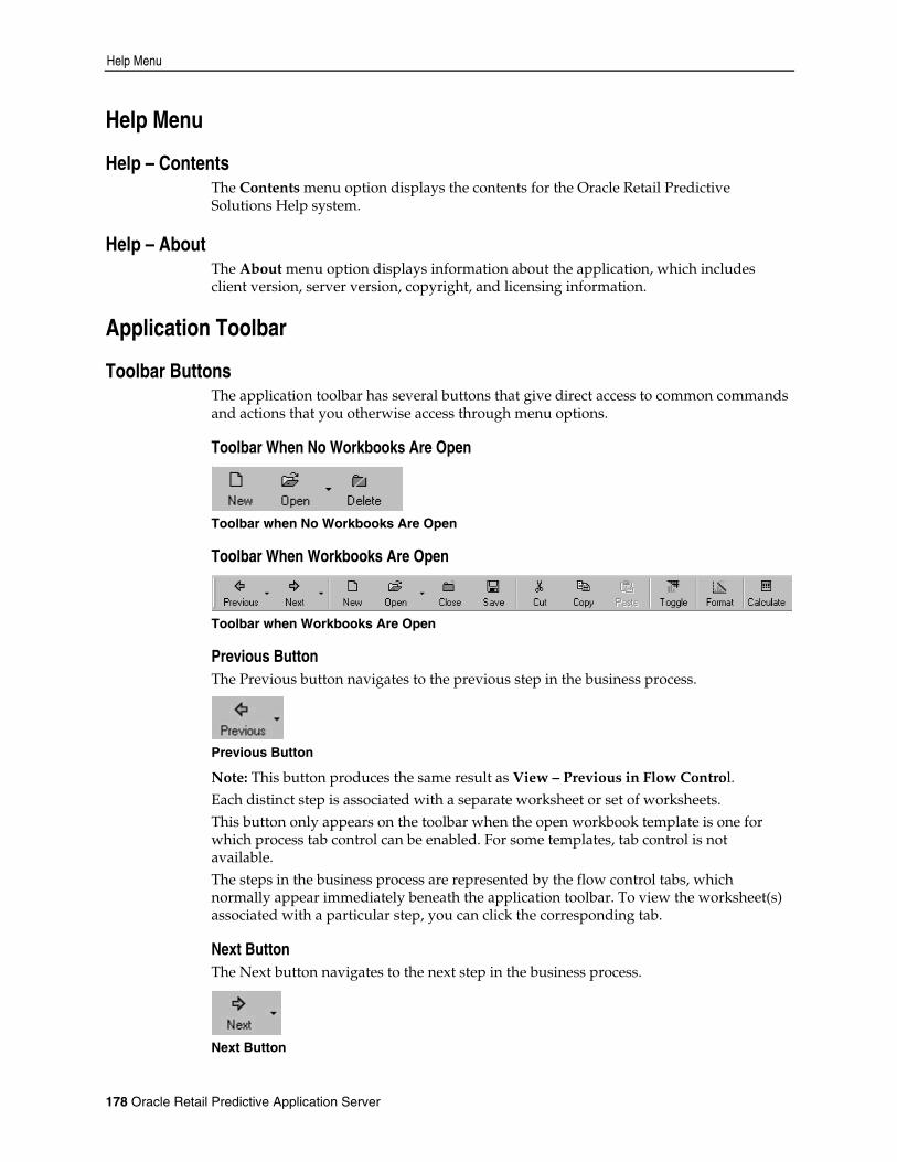
Help Menu
178 Oracle Retail Predictive Application Server
Help Menu
Help – Contents The Contents menu option displays the contents for the Oracle Retail Predictive Solutions Help system.
Help – About The About menu option displays information about the application, which includes client version, server version, copyright, and licensing information.
Application Toolbar
Toolbar Buttons The application toolbar has several buttons that give direct access to common commands and actions that you otherwise access through menu options.
Toolbar When No Workbooks Are Open
Toolbar when No Workbooks Are Open
Toolbar When Workbooks Are Open
Toolbar when Workbooks Are Open
Previous Button The Previous button navigates to the previous step in the business process.
Previous Button
Note: This button produces the same result as View – Previous in Flow Control. Each distinct step is associated with a separate worksheet or set of worksheets. This button only appears on the toolbar when the open workbook template is one for which process tab control can be enabled. For some templates, tab control is not available. The steps in the business process are represented by the flow control tabs, which normally appear immediately beneath the application toolbar. To view the worksheet(s) associated with a particular step, you can click the corresponding tab.
Next Button The Next button navigates to the next step in the business process.
Next Button

Application Toolbar
Appendix: Using RPAS Menus and Toolbars 179
Note: This button produces the same result as View – Next in Flow Control.
Each distinct step is associated with a separate worksheet or set of worksheets. This button only appears on the toolbar when the open workbook template is one for which process tab control can be enabled. For some templates, tab control is not available. The steps in the business process are represented by the flow control tabs, which normally appear immediately beneath the application toolbar. To view the worksheet(s) associated with a particular step, click on the corresponding tab.
New Workbook Button Use the New Workbook button to create a new workbook.
New Workbook Button
Note: Clicking this button is the same action as choosing File – New.
The New dialog appears and allows you to choose a workbook template.
New Dialog Box
This toolbar option is always available, but if you select it while a workbook is already open, you will be prompted to close the current workbook before building the new one.

Application Toolbar
180 Oracle Retail Predictive Application Server
Open Workbook Button Use the Open workbook button to open an existing workbook.
Open Workbook Button
Note: Clicking this button is the same action as choosing File– Open.
The Open dialog is displayed from which you choose a workbook from a list of those available.
Open Workbook Dialog
To bypass the Open dialog and quickly select a workbook to open, click on the small arrow to the right of the Open toolbar button. This arrow produces list of available workbooks from which you can choose one to open. This toolbar option is always available, but if you select it while a workbook is open, you will be prompted to close the current workbook before opening another.
Delete Workbook Button Use the Delete button to delete a workbook.
Delete Button
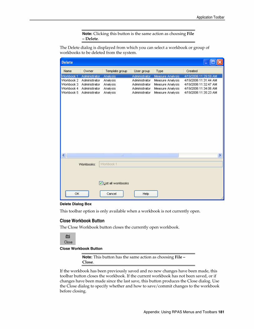
Application Toolbar
Appendix: Using RPAS Menus and Toolbars 181
Note: Clicking this button is the same action as choosing File – Delete.
The Delete dialog is displayed from which you can select a workbook or group of workbooks to be deleted from the system.
Delete Dialog Box
This toolbar option is only available when a workbook is not currently open.
Close Workbook Button The Close Workbook button closes the currently open workbook.
Close Workbook Button
Note: This button has the same action as choosing File – Close.
If the workbook has been previously saved and no new changes have been made, this toolbar button closes the workbook. If the current workbook has not been saved, or if changes have been made since the last save, this button produces the Close dialog. Use the Close dialog to specify whether and how to save/commit changes to the workbook before closing.
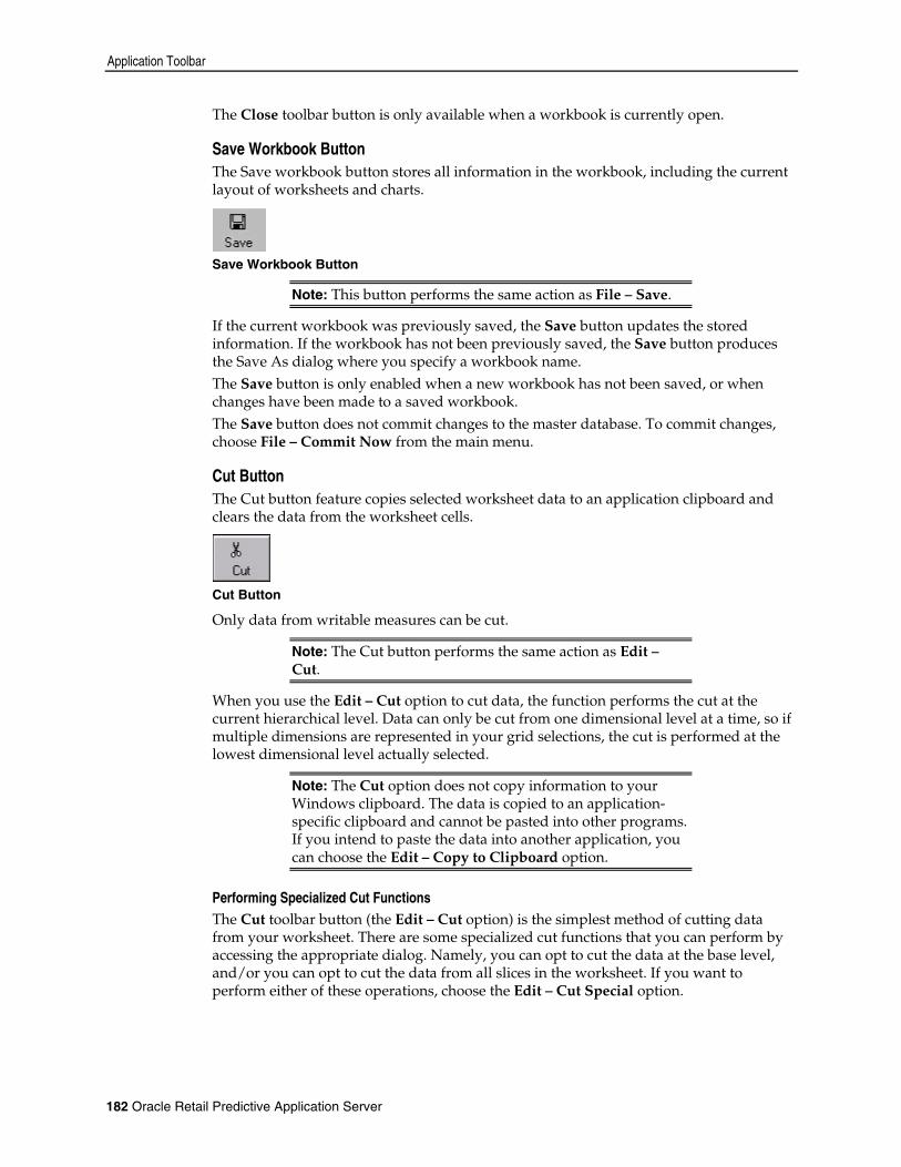
Application Toolbar
182 Oracle Retail Predictive Application Server
The Close toolbar button is only available when a workbook is currently open.
Save Workbook Button The Save workbook button stores all information in the workbook, including the current layout of worksheets and charts.
Save Workbook Button
Note: This button performs the same action as File – Save.
If the current workbook was previously saved, the Save button updates the stored information. If the workbook has not been previously saved, the Save button produces the Save As dialog where you specify a workbook name. The Save button is only enabled when a new workbook has not been saved, or when changes have been made to a saved workbook. The Save button does not commit changes to the master database. To commit changes, choose File – Commit Now from the main menu.
Cut Button The Cut button feature copies selected worksheet data to an application clipboard and clears the data from the worksheet cells.
Cut Button
Only data from writable measures can be cut.
Note: The Cut button performs the same action as Edit – Cut.
When you use the Edit – Cut option to cut data, the function performs the cut at the current hierarchical level. Data can only be cut from one dimensional level at a time, so if multiple dimensions are represented in your grid selections, the cut is performed at the lowest dimensional level actually selected.
Note: The Cut option does not copy information to your Windows clipboard. The data is copied to an application-specific clipboard and cannot be pasted into other programs. If you intend to paste the data into another application, you can choose the Edit – Copy to Clipboard option.
Performing Specialized Cut Functions The Cut toolbar button (the Edit – Cut option) is the simplest method of cutting data from your worksheet. There are some specialized cut functions that you can perform by accessing the appropriate dialog. Namely, you can opt to cut the data at the base level, and/or you can opt to cut the data from all slices in the worksheet. If you want to perform either of these operations, choose the Edit – Cut Special option.

Application Toolbar
Appendix: Using RPAS Menus and Toolbars 183
Copy Button The Copy button copies selected worksheet data to an application clipboard.
Copy Button
Note: This button performs the same action as choosing Edit – Copy.
The Copy function is typically used with the Paste function to speed the process of populating data cells in a worksheet. When you click the Copy button, the system performs the copy at the current hierarchical level. Data can only be copied from one dimensional level at a time, so if multiple dimensions are represented in your grid selections, the copy is performed at the lowest dimensional level actually selected. Unlike the Cut function, Copy does not clear the data from the copied cells.
Note: The Copy command does not copy information to your Windows clipboard. The data is copied to an application-specific clipboard and cannot be pasted into other programs. If you intend to paste the data into another application, you can choose the Edit – Copy to Clipboard command.
Performing Specialized Copy Functions Using the Copy toolbar button (the Edit – Copy command) is the simplest method of copying data in your worksheet. There are some specialized copy functions that you can perform by accessing the appropriate dialog. Namely, you can opt to copy the data at the base level, and/or you can opt to copy the data from all slices in the worksheet. If you want to perform either of these operations, choose the Edit – Copy Special function.
Paste Button The Paste button paste data into measures.
Paste Button
Note: This button performs the same action as choosing Edit – Paste.
This toolbar button is only enabled after you have placed data on the application clipboard by using the Cut, Cut Special, Copy, or Copy Special function. The Paste option pastes the data that was last placed on the system clipboard into the selected cells. Select the cells that you want to paste data into, and click Paste. Data can only be pasted into writable measures.

Application Toolbar
184 Oracle Retail Predictive Application Server
Note: The Paste command does not paste data from your Windows clipboard. This command only pastes data from an application-specific clipboard, and it cannot be used to import data from another application. If you want to paste copied data from another program, you must choose the Edit – Paste from Clipboard command.
Calculate Button The Calculate button submits a queue of data changes to the server for processing.
Calculate Button
Note: This button has the same action as selecting the Edit – Calculate Now menu option.
This button is only enabled when the system is in Manual (Deferred) Calculation mode. Queued changes are executed in the order that they were made.
Update Button The Update button recalculates all sort attributes and dimension splits displayed in the workbook based on user edits since the attribute or dimension split was applied to the data.
Update Button
Toggle View Button The Toggle button toggles the display of worksheet data between Grid view and Chart view.
Toggle Button
Note: This button has the same action as choosing View – Chart or View – Grid.
Format Button When viewing your worksheet in Grid mode, the Format button displays the Format Options dialog, which allows you to customize settings for grid features.

Application Toolbar
Appendix: Using RPAS Menus and Toolbars 185
Format Options Dialog Box - Grid Tab
Format Button
Note: Clicking this button is the same action as choosing Format – Grid.
The Format Options dialog allows you to perform such functions as: Customize the display of horizontal and vertical gridlines Specify the text color, fill color, font, and alignment of cells and labels Specify a color scheme for the grid background, deferred calculation cells, read only
cells, and read/write cells Customize formatting for exception values Specify prefixes, suffixes, and scale factors to facilitate data entry
When viewing your worksheet in Chart Mode, the Format button displays the Chart FX Properties dialog, which allows you to customize settings for chart features.
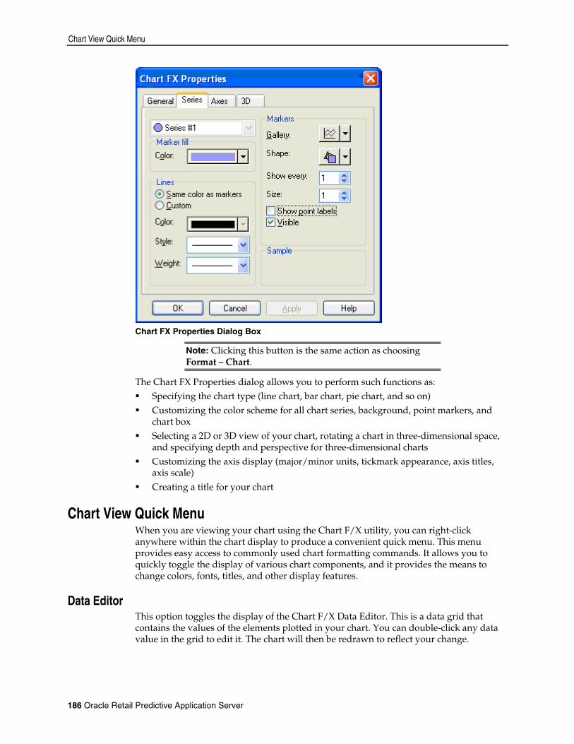
Chart View Quick Menu
186 Oracle Retail Predictive Application Server
Chart FX Properties Dialog Box
Note: Clicking this button is the same action as choosing Format – Chart.
The Chart FX Properties dialog allows you to perform such functions as: Specifying the chart type (line chart, bar chart, pie chart, and so on) Customizing the color scheme for all chart series, background, point markers, and
chart box Selecting a 2D or 3D view of your chart, rotating a chart in three-dimensional space,
and specifying depth and perspective for three-dimensional charts Customizing the axis display (major/minor units, tickmark appearance, axis titles,
axis scale) Creating a title for your chart
Chart View Quick Menu When you are viewing your chart using the Chart F/X utility, you can right-click anywhere within the chart display to produce a convenient quick menu. This menu provides easy access to commonly used chart formatting commands. It allows you to quickly toggle the display of various chart components, and it provides the means to change colors, fonts, titles, and other display features.
Data Editor This option toggles the display of the Chart F/X Data Editor. This is a data grid that contains the values of the elements plotted in your chart. You can double-click any data value in the grid to edit it. The chart will then be redrawn to reflect your change.

Chart FX Toolbar
Appendix: Using RPAS Menus and Toolbars 187
Legend Box This option toggles the display of the series legend.
Gallery This option provides quick access to the gallery types menu, which allows you to select a new chart type.
Color This option provides quick access to a color palette, which allows you to change the color of a selected chart area. Right-click on a chart area (data series, chart box, background, and so on) to produce the quick menu, and select a new color for that chart area from the color palette.
Edit Title The Edit Title option provides quick access to a text box where you can type or edit the chart title.
Point Labels The Point Labels option toggles the display of point labels (data values corresponding to each marker) in your chart.
Font The Font option provides access to a standard font dialog where you can select or change the font, font style, font size, effects, and color of text in your chart. Right-click on the chart text you want to change, and then select Font from the resulting quick menu to display the Font dialog.
Properties The Properties option opens the Chart F/X Properties dialog.
Note: This menu option has the same result as clicking Format on the main toolbar.
Chart FX Toolbar When you view your worksheet in chart mode, the Chart FX charting utility provides a toolbar that you use to access various formatting and chart manipulation features. Pass your cursor over the toolbar to display the button title in a pop-up caption. If the toolbar is currently hidden and you want to display it, right-click within the chart display area, and select Toolbar from the quick menu.
Chart FX Toolbar

Chart FX Toolbar
188 Oracle Retail Predictive Application Server
Open Chart The Open Chart option allows you to open a previously saved chart.
Save Chart The Save Chart option allows you to save a copy of your chart as an individual file. You then specify the name, location, and file type. Charts may be saved as Chart F/X files, Chart F/X templates (no data), and text files (data only, metafile pictures, or bitmap pictures).
Copy to Clipboard The Copy to Clipboard option allows you to copy your chart to a clipboard that can be used in other applications. You can copy your chart in one of three formats:
bitmap image metafile picture text (data only)
This functionality is particularly useful if you want to embed a copy of your chart in a separate document, such as a Word file. Copy your chart to the clipboard as a bitmap image, and paste the chart into the other application.
Gallery The Gallery option provides quick access to the gallery types menu, which allows you to select a new chart type.
Color The Color option provides quick access to a color palette that allows you to change the color of a selected chart area.
Vertical Grid The Vertical Grid option toggles the display of vertical grid lines in your chart.
Horizontal Grid The Horizontal Grid option toggles the display of horizontal grid lines in your chart.

Chart FX Toolbar
Appendix: Using RPAS Menus and Toolbars 189
Legend Box The Legend Box option toggles the display of the series legend.
Data Editor The Data Editor option toggles the display of the Chart FX Data Editor, which is a data grid that contains the values of the elements plotted in your chart. Double-click any data value in the grid to edit it. The chart will then be redrawn to reflect your change.
Properties The Properties option opens the Chart FX Properties dialog. This menu option has the same result as clicking the Format button on the main application toolbar.
3D/2D The 3D/2D option toggles between two-dimensional and three-dimensional views of your data.
Rotate The Rotate option produces the 3D tab of the Chart FX Properties dialog. On this tab, you can customize the properties of three-dimensional charts, including specialized rotation views. This toolbar button is only enabled when the chart is in 3D mode.
Z-Clustered The Z-Clustered option activates and deactivates z-axis clustering. When you are viewing your chart in 3D mode and this feature is selected, each charted series appears in a separate row along the z-axis.
Zoom The Zoom option allows you to zoom in on a section of your chart and view it at a higher magnification. Click this toolbar button to activate the Zoom feature. Then click and hold the mouse button over a corner of the chart area that you want to enlarge. Drag the cursor to the opposite corner of the area that you want to magnify, and release the mouse button. To return to normal view, click the Zoom button again.

Chart FX Toolbar
190 Oracle Retail Predictive Application Server
Print Preview The Print Preview option opens a dialog that you can use to preview your chart before printing. On this dialog, you can specify options, such as print orientation and margins.
Print The Print option allows you to print copies of your chart.
Tools The Tools option provides a menu of features that can be shown or hidden. Click on any menu item to display it if it is currently hidden, or to hide it if it is currently displayed. Use this button to show and hide the values legend, the series legend, the data editor, the palette bar, and the pattern bar.