OPTIS Labs 2013portal.optis-world.com/WebData/38835_LAB_UG.pdf · 2015-05-21 · Page 8 of 207...
207
OPTIS Labs 2013
Transcript of OPTIS Labs 2013portal.optis-world.com/WebData/38835_LAB_UG.pdf · 2015-05-21 · Page 8 of 207...

OPTIS Labs
2013


Table of Contents
Optical Property Editors ...................................................................................... 6 Surface Optical Property Editors ....................................................................... 6
Overview ............................................................................................... 6 Optical Polished Surface ........................................................................ 13 Perfect Mirror Surface ........................................................................... 13 Unpolished Surface ............................................................................... 13 Simple Scattering Surface Editor ............................................................ 15 Advanced Scattering Surface Editor ........................................................ 16 BSDF - BRDF - Anisotropic Surface Viewer ............................................... 17 Coated Surface .................................................................................... 27 Polarizer Surface Editor ......................................................................... 27 Retro Reflecting Surface Editor ............................................................... 30 DOE and Thin Lens Surface Editor .......................................................... 31 Grating Surface Editor ........................................................................... 35 Fluorescent Surface Editor ..................................................................... 36 Rendering Surface Editor ....................................................................... 37 LCD Surface ......................................................................................... 39 Rough Mirror Surface Editor ................................................................... 40 View ................................................................................................... 41 Tools .................................................................................................. 43 Others Options ..................................................................................... 48
Spectrum Editor ........................................................................................... 49 Using the Spectrum Editor ..................................................................... 49 Parameters of a Spectrum ..................................................................... 50 Color Rendering Index .......................................................................... 50 Spectrum Generation ............................................................................ 51
User Material Editor ...................................................................................... 52 Using the User Material Editor ................................................................ 52 Parameters of a User Material ................................................................ 53 Material Color ...................................................................................... 61 Editing the Preferences ......................................................................... 63
Labs .................................................................................................................. 64 Photometric Calc .......................................................................................... 64
Using Photometric Calc .......................................................................... 64 Parameters of Photometric Calc .............................................................. 64
Virtual 3D Photometric Lab ............................................................................ 65 Using Virtual 3D Photometric Lab ........................................................... 65 Managing the Display ............................................................................ 66 3D Map Post-Processing ........................................................................ 66 Surface and Section Analysis ................................................................. 67 Editing the Preferences ......................................................................... 69
Virtual Human Vision Lab .............................................................................. 69 Using Virtual Human Vision Lab .............................................................. 69 Importing an Image .............................................................................. 70 Exporting ............................................................................................ 70 Managing the Display ............................................................................ 74 Reading Precision ................................................................................. 76 Analyzing Colorimetric Data ................................................................... 76 Doing Color Management ...................................................................... 77 Look At ............................................................................................... 79 Vision Parameters ................................................................................. 81 Glare Effect ......................................................................................... 86 Doing Time Adaptation .......................................................................... 87 Doing Analysis ..................................................................................... 87 Legibility and Visibility Analysis .............................................................. 89 Using Sun Glasses / Colored Filter .......................................................... 92 Night Vision Goggles ............................................................................. 94 Surface and Section Analysis ................................................................. 95

Virtual Lighting Controller ...................................................................... 98 Editing the Preferences ....................................................................... 100
Virtual Photometric Lab ............................................................................... 100 Using the Virtual Photometric Lab ......................................................... 100 Importing and Exporting...................................................................... 101 Managing the Display .......................................................................... 110 Reading Precision ............................................................................... 111 Analyzing Colorimetric Data ................................................................. 112 Surface and Section Analysis ............................................................... 112 Virtual Lighting Controller .................................................................... 115 Using Sun Glasses or Colored Filter ....................................................... 117 Night Vision Goggles ........................................................................... 117 Editing the Preferences ....................................................................... 119 Managing the Filtering ......................................................................... 119
Virtual Reality Lab ...................................................................................... 121 Virtual Reality Lab Icons ...................................................................... 121 Using Virtual Reality Lab...................................................................... 122 Virtual Lighting Controller .................................................................... 123 Creating an Immersive View ................................................................ 124 Human Vision..................................................................................... 124 Stereo OptisVR ................................................................................... 126 Creating an Observer View .................................................................. 129 Virtual Reality Lab Management ........................................................... 129 MultiScreen ....................................................................................... 130 Using the SIM2 HDR Monitor ................................................................ 140 Virtual Reality Peripheral Network ......................................................... 140
3D Energy Density Lab ................................................................................ 141 Using 3D Energy Density Lab ............................................................... 141 Managing the Display .......................................................................... 142 Volume and Section Analysis ................................................................ 143 Virtual Lighting Controller .................................................................... 144 Editing the Preferences ....................................................................... 145
Viewers ........................................................................................................... 146 Intensity Viewers ....................................................................................... 146
Eulumdat Viewer ................................................................................ 146 IESNA LM-63 Viewer ........................................................................... 147 OPTIS Intensity Viewer ....................................................................... 149 Curves .............................................................................................. 150
Optical Design Viewers ................................................................................ 153 Coupling Efficiency Viewer ................................................................... 153 Gaussian Propagation Viewer ............................................................... 158 Glass Map Viewer ............................................................................... 158 Paraxial Data Viewer ........................................................................... 160 Real Aberrations Coefficients Viewer ..................................................... 167 Real Aberrations Viewer ...................................................................... 170 Spot Diagram Viewer .......................................................................... 172
Ray File Tools .................................................................................................. 176 Source Generator ....................................................................................... 176
Using the Source Generator ................................................................. 176 Parameters ........................................................................................ 176 Parameters of Position and Orientation .................................................. 183
Post-Processing .......................................................................................... 184 Intensity Distribution Post-processing ................................................... 184 XMP Map Post- processing ................................................................... 185
Ray File Editor ........................................................................................... 188 Using the Ray File Editor ..................................................................... 189 Importing and Exporting...................................................................... 189 Using Data Downloaded from OSRAM Opto Semiconductors ..................... 190 Parameters of Ray File Editor ............................................................... 192

Preferences ..................................................................................................... 194 Monitor ..................................................................................................... 194 Colorimetry ............................................................................................... 195 Printing ..................................................................................................... 195 Spectrometer ............................................................................................. 195 Virtual Photometric Lab ............................................................................... 196 Directories ................................................................................................. 196 3D View .................................................................................................... 196 Virtual 3D Photometric Lab .......................................................................... 198 Devices Preferences .................................................................................... 199 Real Time .................................................................................................. 199 TFCalc....................................................................................................... 199
Index .............................................................................................................. 200

Page 6 of 207 OPTIS Labs User Guide
OPTICAL PROPERTY EDITORS
Surface Optical Property Editors
Overview
Surfaces Overview
You must create a geometry before applying optical properties.
Surfaces describe light's behavior when hitting the surface.
When the light hits the surface, three occurrences may happen: Light is absorbed, reflected or
transmitted.
With the surface editor you can parameterize these behaviors with regards to the wavelength and the
polarization.
You can then create your own coated surface filling in a table with your absorption and transmission
coefficients for each wavelength, and polarization.
Light Behavior Models
For transmission and reflection, light behavior is described with a combination of three models.
With these models you can create very precise surface taking into account that you can use them to
define light's behavior with regards to wavelength and polarization.
SPECULAR MODEL
Specular reflection on a surface
Rays propagate following the Snell -
Descartes law. The proportion of
transmitted and reflected rays is given by
the Fresnel laws (Optical polished and
Scattering models).
LAMBERTIAN MODEL
Lambertian reflection and
transmission on a surface.
The probability to be reflected in a given
direction is the same for all the direction
of the space.

Optical Property Editors Page 7 of 207
GAUSSIAN MODEL
Reflection: Gaussian (10%) and
Lambertian (90%).
The light has a Gaussian probability to be
reflected with a particular angle around
the main direction defined by Snell -
Descartes laws.
BRDF, BTDF, BSDF, Anisotropic Measurement Models
MODEL PARAMETERS REMARKS USE
ADVANCED SCATTERING SURFACE
Theta incident Reflection and/or transmission
For surfaces that fits well
the Gaussian /
Lambertian model
Wavelength Not anisotropic (no dependency
with Phi incident)
Specular, Gaussian and
Lambertian for
reflection &
transmission
Fitted data
ANISOTROPIC SCATTERING SURFACE
Theta, Phi incident Reflection and/or transmission
For surfaces that fits well
the Gaussian /
Lambertian model
Specular, Gaussian and
Lambertian for
reflection &
transmission
Anisotropic (dependency with
Phi incident)
Reflection/Transmissio
n spectrum Fitted data
Vector for orientation Same colors for reflection and
transmission
COMPLETE SCATTERING SURFACE
Theta incident Reflection only
General reflective
surfaces Iridescent
surfaces
Theta, Phi reflection
Wavelength
Not anisotropic (no dependency
with Phi incident) Polarization | and //
both for incidence and
reflection
SIMPLE BSDF
Theta incident - Theta,
Phi reflection/
transmission - 1
Reflection/Transmissio
n spectrum
Reflection and/or transmission
- Not anisotropic (no
dependency with Phi incident) -
Same colors for reflection and
transmission
General isotropic
reflective/transmissive
surfaces (same colors for
reflection and
transmission) Not for
iridescent surfaces
ANISOTROPIC BSDF
Theta, Phi incident Reflection and/or transmission
General isotropic /
anisotropic reflective /
transmissive surfaces. Not
for iridescent surfaces.
Theta, Phi
reflection/transmission
Anisotropic (dependency with
Phi incident)
1 Reflection spectrum Different colors for reflection
and transmission
1 Transmission
spectrum
Does work for isotropic
surfaces as well

Page 8 of 207 OPTIS Labs User Guide
MODEL PARAMETERS REMARKS USE
Vector for orientation
To get a very precise description, you can use the Complete Scattering Surface (BRDF), BSDF Surface
or Anisotropic BSDF Surface which enables the description of almost every isotropic surface.
Complete Scattering Surface
Polarization
Polarization is linked with the physical nature of a photon. It is an electromagnetic wave like radio,
radar, X rays or gamma rays. The difference is just a question of wavelength. A wave is something
vibrating, in the case of a piano or a guitar, it is a cord. When talking about a photon, it is an
electromagnetic field (an electric and a magnetic field which are vibrating together).
In our software, we only take into account the electric field as the magnetic field can be deduced from
it in materials we are using for light propagation.
This electric field is vibrating in a plane which is orthogonal to the photon's direction and it describes
an ellipse centered on this direction.
Polarization is this ellipse defined by its orientation, ellipticity and rotation sense.
Birefringent materials, polarizer surface or optical polished surfaces (Fresnel) are using the
polarization.
Lambertian reflection is depolarizing. It converts polarized photons into unpolarized ones by changing
randomly its polarization while processing the reflection.
Application
The polarization is the main physical property LCDs are working with. LCDs are used together with
polarizer.
According to the applied voltage, they rotate or not the polarization axis of the light by 90°. So when
this light tries to cross the polarizer, it is stopped (black state) in case of a 90° angle of the
polarization axis with the easy axis of the polarizer or transmitted (white state) if this angle is 0°.
We saw that even the simplest surface quality (optical polished) has an effect on polarization. This is
the surface quality used each time one deal with a light guide in automotive (dashboards) or in
telephony (to enlight the keypad for example).
Since such devices are using multiple reflections inside they light guides, it is important to have an
accurate model to describe the light behavior on this surface.
Optical Property Editors Page 9 of 207
It is possible to build a light guide with a birefringent material in order to build a special function for
the polarization. For example, a backlight for a LCD without any polarizer between the backlight and
the LCD reducing the losses due to the polarizer.
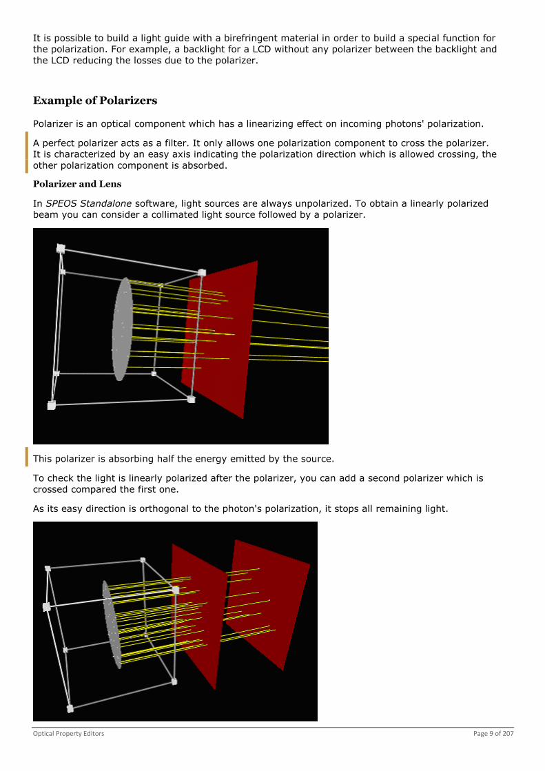
Example of Polarizers
Polarizer is an optical component which has a linearizing effect on incoming photons' polarization.
A perfect polarizer acts as a filter. It only allows one polarization component to cross the polarizer.
It is characterized by an easy axis indicating the polarization direction which is allowed crossing, the
other polarization component is absorbed.
Polarizer and Lens
In SPEOS Standalone software, light sources are always unpolarized. To obtain a linearly polarized
beam you can consider a collimated light source followed by a polarizer.
This polarizer is absorbing half the energy emitted by the source.
To check the light is linearly polarized after the polarizer, you can add a second polarizer which is
crossed compared the first one.
As its easy direction is orthogonal to the photon's polarization, it stops all remaining light.

Page 10 of 207 OPTIS Labs User Guide
Now a lens can be inserted between both polarizers. Its influence on polarization can be seen by
setting an irradiance sensor.
A known figure on the simulation's result can be seen.
The minimum of the energy is on the axis of each polarizer.
The maximum of the energy is at 45° between each axis.
Multiple Polarizer
Crossed polarizer (angle between easy axes is 90°) are stopping the light. This next example is a
successive polarizer with easy axes angles different from 90°.

Optical Property Editors Page 11 of 207
Following picture gives the transmission in function of the angle between the easy axis.
In the Polarizer and Lens example, without the lens the light is completely stopped. In this example,
you can replace the lens by a polarizer whose easy axis is at 45° from the two others.
The light crossing the first polarizer in linearly polarized at 45° from the second one.
So the second polarizer only stops a part of the light and transmits photons whose polarization is 45°
from the last polarizer's easy axis. This makes that the last polarizer doesn't stop all the remaining
light. Moreover, the polarization of the light which goes out of the system is orthogonal to the easy
axis of the first polarizer. This system acts as a polarization rotation tool. We could achieve a better
transmission coefficient by making more rotation steps (here we made two 45° steps).
This is basically the way LCDs are rotating the polarization: The molecules in the liquid crystal may be
considered as small polarizer and their orientation is evolving along the light path making the
polarization rotate progressively reducing losses.
Brewster Angle
Even a simple glass has an influence on polarization. Its optical polished surface behavior on light is
described by Fresnel's law. This law is different for S and P polarization.

Page 12 of 207 OPTIS Labs User Guide
S polarization
P polarization
Parallel and perpendicular (orthogonal) refers to the electric field vector of the polarization and the
light incidence plane.
Parallel = P polarization = TM (transverse magnetic).
Orthogonal = Perpendicular = S polarization = TE (transverse electric).
S and P are named belong to the German words Senkrecht and Parallel.
We can see on the P polarization curve that there is an angle which only reflects S polarization. As a
consequence, for this angle, a reflected beam has same properties as a beam which crossed a
polarizer. Its polarization is linear. This angle is called Brewster angle.
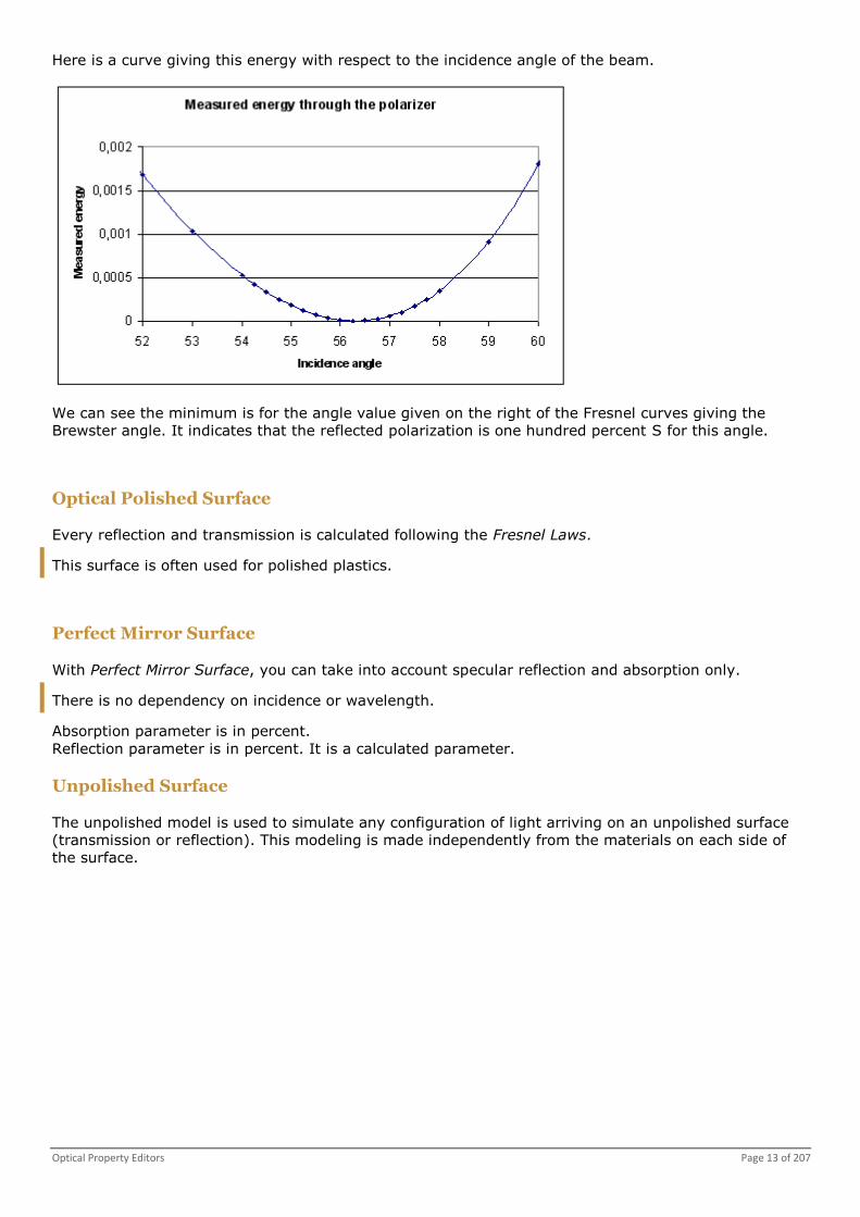
We can check this by making the reflected beam go through a polarizer and measure the energy that
crosses the polarizer which only selects P polarization.
Optical Property Editors Page 13 of 207
Here is a curve giving this energy with respect to the incidence angle of the beam.
We can see the minimum is for the angle value given on the right of the Fresnel curves giving the
Brewster angle. It indicates that the reflected polarization is one hundred percent S for this angle.
Optical Polished Surface
Every reflection and transmission is calculated following the Fresnel Laws.
This surface is often used for polished plastics.
Perfect Mirror Surface
With Perfect Mirror Surface, you can take into account specular reflection and absorption only.
There is no dependency on incidence or wavelength.
Absorption parameter is in percent.
Reflection parameter is in percent. It is a calculated parameter.
Unpolished Surface
The unpolished model is used to simulate any configuration of light arriving on an unpolished surface
(transmission or reflection). This modeling is made independently from the materials on each side of
the surface.

Page 14 of 207 OPTIS Labs User Guide
On the following drawing, you can see a configuration that cannot be modeled by a BSDF. Indeed, with
a BSDF model you model a whole film, with its two diopters, whereas, with the unpolished surface
model, you can characterize only the diffusion of a single diopter. This type of model is close to the
BSDF model, but only the normal distribution is kept, and the model adapts to the underlying material
refraction indices using Fresnel formula. Material properties are computed during the simulation
according to the VOP of the OPTIS software used.
This technology can apply to any unpolished surface, for instance surfaces treated by electro-erosion,
wet etching or sandblasting for instance.
Example of an unpolished surface (diffuse surface).
.unpolished files are measured with OMS4. You can get files either:
from measurements made on materials from libraries like VDI or Charmilles.
from specific measurements made on request.
For specific measurements, please contact your OPTIS sales representative (http://www.optis-
world.com/contact.htm).
Typical application for this type of surface state is the modeling of a diffuse surface in a light guide.
Propagation of light in a light guide.

Optical Property Editors Page 15 of 207
For additional information concerning this surface model, you can view Simulation.
Simple Scattering Surface Editor
With Simple Scattering Surface Editor, you can simulate the surface's behavior with the classical model
(specular, Lambertian, Gaussian) for both transmitted and reflected rays.
You can modulate the Gaussian angle in respect of the parallel or perpendicular plan.
Using the Simple Scattering Surface Editor
1. From Start menu, click All Programs, OPTIS, OPTIS Labs, Optical Property Editors, Surface
Optical Property Editors, Simple Scattering Surface Editor.
-Or-
1. Click Simple Scattering surface .
A window appears.
You can create, open or save a surface. In this case you can save your surface as a
.simplescattering file.
2. Set the parameters see page 15.
You can view Scattering surface curve see page 41.
You can edit surface properties see page 43.
You can edit preferences see page 47.
Parameters of a Simple Scattering Surface
The surface quality does not depend on incidence angle, polarization... It works according reflection
only, transmission only, or reflection and transmission.
A global absorption is when there is no dependency with the wavelength.
A Lambertian reflection is when there is dependency with the wavelength.
In all cases, when a photon hits a surface with this surface state, the surface absorption and the
percentages of reflection and transmission are first computed according to the photon incidence
and wavelength.
In the case of propagation with photon weight, the absorption is subtracted to the photon energy.
The photon is propagated after the interaction with the surface with the new energy.
In the case of propagation without photon weight, the absorption is the probability for the photon
to be absorbed.
A random number is then computed in order to choose the interaction type (reflection or transmission,
specular, Gaussian or Lambertian, and absorption in the case of propagation without photon weight)
and their respective probabilities.
Calculations take into account incidence following the Snell law.
Absorption
In Absorption box, you must type the value of the absorbed energy in percent.
When you open a Lambertian reflection you can describe a colored surface. In this case Absorption
parameter is not available.
Non Absorption
This Non absorption box gives the non absorbed energy.
Non absorption = P = (100 - Absorption).

Page 16 of 207 OPTIS Labs User Guide
P is computed and used as following:
Reflection or transmission only: The percentages of Lambertian, Gaussian or specular reflection (or
transmission) are percentages of P. All other percentages of transmission (or reflection) are set to
0.
Reflection and transmission:
If Use Fresnel is selected, the Fresnel law gives the percentages of reflection (Rf) and
transmission (Tf) according to the photon incidence and wavelength.
If User is selected, you must type the percentage of reflection (Rf) and the transmission (Tf) is
computed as 100-Rf. The global percentages are respectively:
Rt = P * Rf / 100
Tt = P * Tf / 100
Then Lambertian, Gaussian or specular percentages are percentages of Rt and Tt.
Reflection
You can select the Reflection check box.
In Reflection gaussian angle box, you must type the angle value of the gaussian diffusion in
reflected light in degree.
In Lambertian box, you must type the percentage of Lambertian diffusion in reflected light.
In Gaussian box, you must type the percentage of Gaussian diffusion in reflected light.
In Specular box, you must type the percentage of specular reflection in reflected light.
Transmission
You can select the Transmission check box.
In Lambertian box, you must type the percentage of Lambertian diffusion in transmitted light.
In Gaussian box, you must type the percentage of Gaussian diffusion in transmitted light.
In Specular box, you must type the percentage of specular reflection in transmitted light.
In Transmission gaussian angle box, you must type the angle value of Gaussian diffusion in
transmitted light in degree.
Use Fresnel / User
If both Reflection and Transmission check boxes are selected, you can view Use Fresnel and User.
If you select Use Fresnel, the ratio between reflected energy and transmitted energy follows the
optical Fresnel laws. Otherwise reflection and transmission percentages are used.
If you select User, you must type the reflection percentage.
Advanced Scattering Surface Editor
With Advanced Scattering Surface Editor, you can define more complex surface quality which can
depend on incidence angle, polarization...
Two additional effects compared to the Simple Scattering Surface Editor are the dependence of the
diffusion on incidence angle and of the diffusion on spectrum (colored surface).
Transmitted and reflected rays are described with a specular behavior, a Lambertian diffusion and a
Gaussian diffusion. Calculations take into account wavelength and incidence, and you can define up to
eleven parameters to give a precise description of the ray behavior.
This editor is commonly used with measurements.
Using the Advanced Scattering Surface Editor
1. From Start menu, click All Programs, OPTIS, OPTIS Labs, Optical Property Editors, Surface
Optical Property Editors, Advanced Scattering Surface Editor.

Optical Property Editors Page 17 of 207
-Or-
1. Click Advanced Scattering surface .
A window appears.
You can create, open or save a surface. In this case you can save your surface as a .scattering
file.
2. Set the parameters see page 17.
You can view Scattering surface curve see page 41.
You can edit surface properties see page 43.
You can edit preferences see page 47.
You can get some help to generate the surface see page 47.
Parameters of an Advanced Scattering Surface
For each wavelength and each incidence, you have to define ten parameters.
Absorption is a self-calculating value.
You must type a specular reflection value in percent.
You must type a Lambertian diffusion value around reflected ray in percent.
You must type a Gaussian diffusion value around reflected ray in percent.
You must type a Gaussian angle value in the incidence plane in degree.
You must type a Gaussian angle value in the perpendicular plane in degree.
You must type a specular transmitted ray value in percent.
You must type a Lambertian diffusion value around transmitted ray in percent.
You must type a Gaussian diffusion value around transmitted ray in percent.
You must type a Gaussian angle value in the incidence plane in degree.
You must type a Gaussian angle value in the perpendicular plane in degree.
If needed, you can Add incidence or Delete incidence .
If needed, you can Add wavelength or Delete wavelength .
BSDF - BRDF - Anisotropic Surface Viewer
With BSDF - BRDF - Anisotropic Surface viewer, you can display the 3D view of any BSDF, BRDF,
Anisotropic scattering or Anisotropic BSDF surface files.
Using the BSDF - BRDF - Anisotropic Surface Viewer
1. From Start menu, click All Programs, OPTIS, OPTIS Labs, Optical Property Editors, Surface
Optical Property Editors, BSDF - BRDF - Anisotropic Surface Viewer.
-Or-
1. Click BSDF - BRDF - Anisotropic surface .
A window appears.
2. Click File, Open... and select a supported file.
Supported files are Simple BSDF see page 19, Anisotropic BSDF see page 19, Complete scattering
see page 23, BSDF180 see page 25 , unpolished see page 13 and coated see page 27 files.
3. Set the parameters see page 18.

Page 18 of 207 OPTIS Labs User Guide
You can save a surface.
You can save the surface as measure file saving it in a binary compressed format. Be aware that
this can not be undone.
You can build BSDF180 surface see page 25.
You can export to conoscopic map see page 26.
You can edit surface properties see page 43.
You can edit preferences see page 47.
Parameters of Scattering Surface
Display
By selecting the View shading check box, you can display a shading view of the intensity
envelope.
By selecting the View Mesh check box, you can display the intensity envelope with wireframe.
By selecting the Pure Lambertian curve check box, you can display the pure Lambertian curve.
By selecting the Incident direction check box, you can display the incident direction.
By selecting the Tangent plane check box, you can display the tangent plane.
By selecting the Axis System check box, you can display the axis System.
By selecting the Decorations check box, you can display the 3D view tool.
For more details, you can view Using 3D view tool.
By selecting the BRDF check box, you can display the BRDF.
By selecting the Probability density check box, you can display the probability density.
By selecting the Logarithmic View check box, you can display the logarithmic view.
By clicking , you can edit 3D view preferences see page 196.
Incidence
With Incidence group box, you can view the incidence dependency (theta and phi).
Wavelength
With Wavelength group box, you can view the wavelength dependency.

Optical Property Editors Page 19 of 207
Optical Properties
With Optical properties group box, you can modify optical properties.
Anisotropy Vector
With Anisotropy vector group box, you can modify the anisotropic vector for anisotropic surfaces.
Simple BSDF Surface
From OPTIS Labs 2012 release, it is strongly recommended to use the Anisotropic BSDF Surface see
page 19 model instead of Simple BSDF Surface model.
Anisotropic BSDF Surface
Anisotropic BSDF Surface Overview
You can measure surface properties with OMS² or OMS4 software.
For more information on the use of this model, you can view Parameters of Interpolation Enhancement.
With Anisotropic BSDF Surface, you can simulate both isotropic and anisotropic surfaces from
goniometric measurement data.
The model handles BSDF as well as BRDF only or BTDF only surfaces.
Anisotropic BSDF uses an approximation to deal with the spectrum.
With following diagram you can view angle definitions for incoming and outgoing directions according
to the surface normal (Z) and the fixed anisotropic vector.
The incoming photon is displayed in blue.
Z vector Surface normal
X vector Constructed for a given incoming photon as the projection of its
direction on the surface plane
Y Computed from X and Z
Anisotropic vector Directs the surface when the vector given in the file is not in the tangent
plane at the impact point, an orthogonal projection of it is used instead
Anisotropic angle Phi_i Angle between X and the anisotropic vector using trigonometrical
convention (Phi_i is positive on the diagram)
Theta_i Incidence angle
Output direction
(Theta_o, Phi_o)
Displayed in red and is given using standard spherical coordinates in the
X,Y,Z axis system
Page 20 of 207 OPTIS Labs User Guide
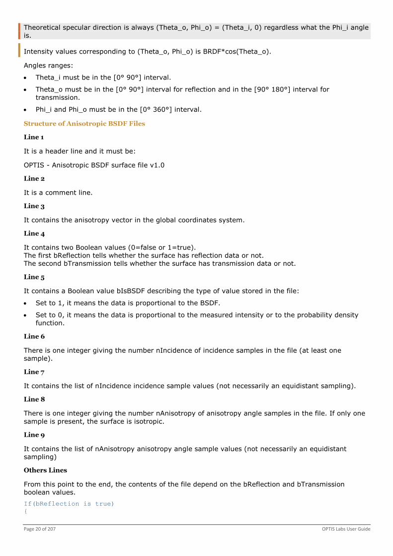
Theoretical specular direction is always (Theta_o, Phi_o) = (Theta_i, 0) regardless what the Phi_i angle
is.
Intensity values corresponding to (Theta_o, Phi_o) is BRDF*cos(Theta_o).
Angles ranges:
Theta_i must be in the [0° 90°] interval.
Theta_o must be in the [0° 90°] interval for reflection and in the [90° 180°] interval for
transmission.
Phi_i and Phi_o must be in the [0° 360°] interval.
Structure of Anisotropic BSDF Files
Line 1
It is a header line and it must be:
OPTIS - Anisotropic BSDF surface file v1.0
Line 2
It is a comment line.
Line 3
It contains the anisotropy vector in the global coordinates system.
Line 4
It contains two Boolean values (0=false or 1=true).
The first bReflection tells whether the surface has reflection data or not.
The second bTransmission tells whether the surface has transmission data or not.
Line 5
It contains a Boolean value bIsBSDF describing the type of value stored in the file:
Set to 1, it means the data is proportional to the BSDF.
Set to 0, it means the data is proportional to the measured intensity or to the probability density
function.
Line 6
There is one integer giving the number nIncidence of incidence samples in the file (at least one
sample).
Line 7
It contains the list of nIncidence incidence sample values (not necessarily an equidistant sampling).
Line 8
There is one integer giving the number nAnisotropy of anisotropy angle samples in the file. If only one
sample is present, the surface is isotropic.
Line 9
It contains the list of nAnisotropy anisotropy angle sample values (not necessarily an equidistant
sampling)
Others Lines
From this point to the end, the contents of the file depend on the bReflection and bTransmission
boolean values.
If(bReflection is true)
{
Optical Property Editors Page 21 of 207
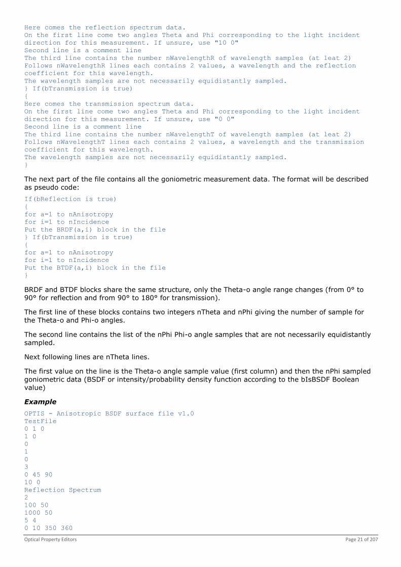
Here comes the reflection spectrum data.
On the first line come two angles Theta and Phi corresponding to the light incident
direction for this measurement. If unsure, use "10 0"
Second line is a comment line
The third line contains the number nWavelengthR of wavelength samples (at leat 2)
Follows nWavelengthR lines each contains 2 values, a wavelength and the reflection
coefficient for this wavelength.
The wavelength samples are not necessarily equidistantly sampled.
} If(bTransmission is true)
{
Here comes the transmission spectrum data.
On the first line come two angles Theta and Phi corresponding to the light incident
direction for this measurement. If unsure, use "0 0"
Second line is a comment line
The third line contains the number nWavelengthT of wavelength samples (at leat 2)
Follows nWavelengthT lines each contains 2 values, a wavelength and the transmission
coefficient for this wavelength.
The wavelength samples are not necessarily equidistantly sampled.
}
The next part of the file contains all the goniometric measurement data. The format will be described
as pseudo code:
If(bReflection is true)
{
for a=1 to nAnisotropy
for i=1 to nIncidence
Put the BRDF(a,i) block in the file
} If(bTransmission is true)
{
for a=1 to nAnisotropy
for i=1 to nIncidence
Put the BTDF(a,i) block in the file
}
BRDF and BTDF blocks share the same structure, only the Theta-o angle range changes (from 0° to
90° for reflection and from 90° to 180° for transmission).
The first line of these blocks contains two integers nTheta and nPhi giving the number of sample for
the Theta-o and Phi-o angles.
The second line contains the list of the nPhi Phi-o angle samples that are not necessarily equidistantly
sampled.
Next following lines are nTheta lines.
The first value on the line is the Theta-o angle sample value (first column) and then the nPhi sampled
goniometric data (BSDF or intensity/probability density function according to the bIsBSDF Boolean
value)
Example
OPTIS - Anisotropic BSDF surface file v1.0
TestFile
0 1 0
1 0
0
1
0
3
0 45 90
10 0
Reflection Spectrum
2
100 50
1000 50
5 4
0 10 350 360

Page 22 of 207 OPTIS Labs User Guide
0 0 0 0 0
30 1 0 0 1
45 1 0 0 1
60 1 0 0 1
90 0 0 0 0
5 6
0 15 45 315 345 360
0 0 0 0 0 0 0
30 0 0 0 0 1 0
45 1 0 0 0 0 1
60 0 1 0 0 0 0
90 0 0 0 0 0 0
5 6
0 15 45 315 345 360
0 0 0 0 0 0 0
30 0 0 0 0 0 0
45 1 1 0 0 1 1
60 0 0 0 0 0 0
90 0 0 0 0 0 0
If your anisotropic surface shows a symmetry in its behavior, it is possible to put the data for the [0°
90°] or the [0° 180°] intervals for the Phi_i angle instead of [0° 360°].
For more details, you can view anisotropic BSDF surface examples from
LAB_Anisotropic_BSDF_Surface.zip (../Common/LAB_Anisotropic_BSDF_Surface.zip).
Specular Constant for Anisotropic BSDF
For more information on the use of this model, you can view Parameters of Interpolation Enhancement.
Generally speaking, the directional part of a BRDF is measured with OMS4 and the reflection spectrum
is measured with the integrating sphere. When modeling anisotropic BSDF models, the measure does
not allow to make the difference between the diffuse /lambertian parts and the specular/gaussian
parts. The model applies the color measured with the integrating sphere to the whole BRDF. The result
is that the specular reflection is the same color as the diffuse part, which is often not the case in real
situations. The specular constant model allows to make the difference between the diffuse/lambertian
parts and the specular/gaussian parts for anisotropic BSDF.
As this new model is based on the separation between diffuse and specular data brought by incidence
interpolation, you can only use it on surfaces for which you activate incidence interpolation.
The validity of the model relies on the accuracy of the specular/diffuse separation. Any flaw will result
in calculation errors.
On the following example you can view a sphere with a colored reflection spectrum illumined by a
white source.
Before, the specular highlight had the same spectrum as the diffuse part, both had the same color.

Optical Property Editors Page 23 of 207
With the new model, the specular highlight is white and the diffuse part remains unchanged.
Complete Scattering Surface (BRDF)
You can measure surface properties with OMS² or OMS4 software.
With Complete Scattering Surface (BRDF), you can simulate a BRDF.
This surface is scattering light only in reflection.
Complete Scattering Surface model is new from the OPTIS Labs 2008 release.
Due to file compatibility issues, the file extension is a .bdrf however the file itself reflects a full BSDF
function.
The new model replaces the former one while keeping compatibility by importing the former model
files.
The polarization dependency has been removed.
The Complete Scattering Surface is now able to handle transmission as well as reflection.
Complete scattering is not able to deal with anisotropy.
File Format
The model uses a text format file.
Line 1
It is a header used to discriminate from older file format.
OPTIS - brdf surface file v3.0
Line 2
It is a file description.
Surface description
Line 3
There are two boolean values for reflection and transmission.
1 value is set when there is reflection/transmission.
0 value is set when there is not reflection/transmission.
1 1
Both reflection and transmission example
Line 4
It contains a boolean value.
0 value is set when the data is proportional to intensity.
1 value is set when the data is proportional to BSDF.
Line 5
It contains the number of samples in incidence and in wavelength.
There is a minimum of two incidence samples and two wavelength samples.
2 2

Page 24 of 207 OPTIS Labs User Guide
Line 6
It contains the list of the incidence samples in degree.
0 90
Line 7
It contains the list of the wavelength samples in nanometer.
400 700
Others Lines
The next contain is organized as blocks of data.
The blocks organization is described first, then the blocks contents.
Blocks Organization
if the surface has reflection
{
for I=1 to Incidence Sample Number
{
for W=1 to Wavelength Sample Number
{
Write Reflection Block(I,W)
}
}
}
if the surface has transmission
{
for I=1 to Incidence Sample Number
{
for W=1 to Wavelength Sample Number
{
Write Transmission Block(I,W)
}
}
}
It means the reflection comes first if present and the transmission comes after if present according to
the boolean values from line 3.
Block Content
The first line contains the reflection or transmission coefficient in percent.
50
If 50% of the light is reflected/transmitted
The second line contains the number of samples in theta and the number of samples in phi.
Theta is the polar angle (the poles are on the surface normal direction) its origin is on the reflection
pole.
Phi is the azimuth angle, its origin is defined by the specular reflection.
2 3
On the third line, there is the list of the phi samples.
0 180 3 60
Next, there are as many lines as there are theta samples.
The first value on each line is the theta angle sample value.
Then there is one value per phi sample corresponding to the intensity (or the BSDF depending on
boolean from line 4 of the file.)
0 1 1 1
90 1 1 1
For reflection, theta goes from 0° (normal) to 90° (grazing).
For transmission, theta goes from 90°(grazing) to 180°.

Optical Property Editors Page 25 of 207
The Intensity or BSDF values do not need to be absolute values as the reflection/transmission
coefficient is present at the beginning of each block and is used to normalize the values appropriately.
Anisotropic Scattering Surface
From OPTIS Labs 2012 SP3 release, it is strongly recommended to use the Anisotropic BSDF Surface
see page 19 model instead of Anisotropic Scattering Surface model.
BSDF180 Surface
BSDF180 Overview
You can measure surface properties with OMS² or OMS4 software.
Some optical films have asymmetrical optical properties according to which surface the light interacts
with first.
Two distinct measurements are required to characterize such films.
With BSDF180 surface, you can combine both measurements and orient them to simulate the complete
film behavior.
With BSDF - BRDF - Anisotropic Surface viewer, you can display 3D view of BSDF180 file.
When using BSDF180, you can select .anisotropicBSDF or .brdf file format.
Building BSDF180 Surface
1. Click File, Build BSDF180....
A window appears.
2. In Normal BSDF box, you must browse one BSDF file for the normal direction.
3. In Opposite BSDF box, you must browse one BSDF file for the opposite direction.
Normal BSDF Opposite BSDF

Page 26 of 207 OPTIS Labs User Guide
4. Click OK.
The new BSDF180 file combines both data.
The normal BSDF is observed for Theta varying between 0° and 90° and the opposite BSDF for
Theta varying between 90° and 180°.
Exporting to Conoscopic Map
In conoscopic map, there is one layer per incidence. The map gives selected incidences' reflection
and/or transmission.
1. Click File, Export to conoscopic map....
A window appears.
In Map sampling box, you must enter a map sampling value in pixels.
In Wavelength of conversion box, you must enter a wavelength of conversion value in
nanometers.
In Anisotropic angle of conversion box, you must enter a Anisotropic angle of conversion value
in degrees.
You must select a reflection or transmission type.
2. Browse a Map file.
This is a .xmp format.
3. Click OK.
Change Reflection or Transmission Spectrum
Changing Reflection or Transmission Spectrum
Change reflection or transmission spectrum is only available for anisotropic BSDF files.
1. Click File, Change reflection or transmission spectrum.
A window appears.
2. Set the parameters see page 26.
3. Click OK.
4. Save the file.
Parameters to Change Reflection or Transmission Spectrum
Reflection
In Reflection group box, you can select the check box to set the reflection spectrum.
Optical Property Editors Page 27 of 207
In Theta and Phi boxes, you must then set Theta and Phi values to set the lighting direction used for
the spectrum measurement.
You must then open the corresponding reflection spectrum.
Transmission
In Transmission group box, you can select the check box to set the transmission spectrum.
In Theta and Phi boxes, you must then set Theta and Phi values to set the lighting direction used for
the spectrum measurement.
You must then open the corresponding transmission spectrum.
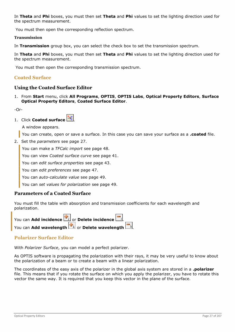
Coated Surface
Using the Coated Surface Editor
1. From Start menu, click All Programs, OPTIS, OPTIS Labs, Optical Property Editors, Surface
Optical Property Editors, Coated Surface Editor.
-Or-
1. Click Coated surface .
A window appears.
You can create, open or save a surface. In this case you can save your surface as a .coated file.
2. Set the parameters see page 27.
You can make a TFCalc import see page 48.
You can view Coated surface curve see page 41.
You can edit surface properties see page 43.
You can edit preferences see page 47.
You can auto-calculate value see page 49.
You can set values for polarization see page 49.
Parameters of a Coated Surface
You must fill the table with absorption and transmission coefficients for each wavelength and
polarization.
You can Add incidence or Delete incidence .
You can Add wavelength or Delete wavelength .
Polarizer Surface Editor
With Polarizer Surface, you can model a perfect polarizer.
As OPTIS software is propagating the polarization with their rays, it may be very useful to know about
the polarization of a beam or to create a beam with a linear polarization.
The coordinates of the easy axis of the polarizer in the global axis system are stored in a .polarizer
file. This means that if you rotate the surface on which you apply the polarizer, you have to rotate this
vector the same way. It is required that you keep this vector in the plane of the surface.

Page 28 of 207 OPTIS Labs User Guide
Using the Polarizer Surface Editor
1. From Start menu, click All Programs, OPTIS, OPTIS Labs, Optical Property Editors, Surface
Optical Property Editors, Polarizer Surface Editor.
-Or-
2. Click Polarizer Surface .
A window appears.
You can create, open, edit and save a new polarizer surface.
In this case you can save your surface as a .polarizer file. New files are always saved in V2.0
version.
You can open, edit or save an existing .polarizer surface.
V1 versions are saved as V1.0 polarizer files, V 2.0 versions are saved as V2.0 polarizer files.
3. Set the parameters see page 28.
You can click to convert directly a V1.0 polarizer file into a V2.0 polarizer file.
You can also view Polarizer Surface V1.0 see page 29 and Polarizer Surface V2.0 see page 30 to create
V 1.0 or V 2.0 polarizer files directly in a text file.
Parameters of a Polarizer Surface
Polarizer Surface V1.0
Open a polarizer surface V1.0 to access this parameters.
Description
Define a name for you polarizer surface.
Easy Axis
It is the easy axis vector.
Set the X, Y, Z values.
Polarizer Surface V2.0
Open an existing polarizer surface V2.0 or create a new polarizer surface to access this parameters.
Description
Define a name for you polarizer surface.
X Axis
It is the X axis vector defined in the global axis system.
Set the X, Y, Z values.
Y Axis
It is the Y axis vector. It has to be perpendicular to the X axis.
Set the X, Y, Z values.
The angle between two axes should be at least equal to 45°.
X axis vector and Y axis vector do not need to be normalized. Vector length can be different than 1.
Values are automatically normalized when saving the surface. You can click to preview the
normalized values.
Jones Matrix
It is the Jones Matrix defined in the X and Y base.

Optical Property Editors Page 29 of 207
In case the Jones Matrix contains complex values, the convention is (a,b) with a the real part and b
the imaginary part.
Polarizer surfaces v2.0 are perfect. There is no loss of energy. Jones matrices are normalized for
calculation.
Jones Matrix Examples
EXAMPLE JONES MATRIX JONES MATRIX IN THE POLARIZER SURFACE V2.0 FILE
Linear polarizer along Ox
1
0
0
0
Linear polarizer along Oy
0
0
0
1
Left circular polarizer
1
(0,1)
(0,-1)
1
Right circular polarizer
1
(0,-1)
(0,1)
1
1/2 is a normalization coefficient avoiding to create energy when the light goes through the
polarizer. As code of the polarizer surface V2.0 file takes into account the normalization, this
coefficient is not required in the Jones Matrix.
Quarter-wave plate with fast axis along
X
1
0
0
(0,1)
Half-wave plate with fast axis along X
1
0
0
-1
No global phase angle difference equal on X and Y is taken into account in theses matrix because
photons' phase is not kept in calculations.
Polarizer Surface V1.0
With Polarizer Surface, you can model a perfect polarizer.
As OPTIS software is propagating the polarization with their rays, it may be very useful to know about
the polarization of a beam or to create a beam with a linear polarization.
The coordinates of the easy axis of the polarizer in the global axis system are stored in a .polarizer
file. This means that if you rotate the surface on which you apply the polarizer, you have to rotate this
vector the same way. It is required that you keep this vector in the plane of the surface.
File Format
Line 1
It is a header line.
OPTIS - Polarizer surface file v1.0
Line 2
It is a comment line.
My polarizer
Line 3
It is the easy axis vector.
1 0 0
Page 30 of 207 OPTIS Labs User Guide
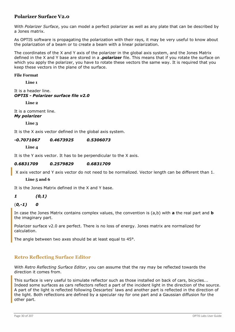
Polarizer Surface V2.0
With Polarizer Surface, you can model a perfect polarizer as well as any plate that can be described by
a Jones matrix.
As OPTIS software is propagating the polarization with their rays, it may be very useful to know about
the polarization of a beam or to create a beam with a linear polarization.
The coordinates of the X and Y axis of the polarizer in the global axis system, and the Jones Matrix
defined in the X and Y base are stored in a .polarizer file. This means that if you rotate the surface on
which you apply the polarizer, you have to rotate these vectors the same way. It is required that you
keep these vectors in the plane of the surface.
File Format
Line 1
It is a header line.
OPTIS - Polarizer surface file v2.0
Line 2
It is a comment line.
My polarizer
Line 3
It is the X axis vector defined in the global axis system.
-0.7071067 0.4673925 0.5306073
Line 4
It is the Y axis vector. It has to be perpendicular to the X axis.
0.6831709 0.2579829 0.6831709
X axis vector and Y axis vector do not need to be normalized. Vector length can be different than 1.
Line 5 and 6
It is the Jones Matrix defined in the X and Y base.
1 (0,1)
(0,-1) 0
In case the Jones Matrix contains complex values, the convention is (a,b) with a the real part and b
the imaginary part.
Polarizer surface v2.0 are perfect. There is no loss of energy. Jones matrix are normalized for
calculation.
The angle between two axes should be at least equal to 45°.
Retro Reflecting Surface Editor
With Retro Reflecting Surface Editor, you can assume that the ray may be reflected towards the
direction it comes from.
This surface is very useful to simulate reflector such as those installed on back of cars, bicycles...
Indeed some surfaces as cars reflectors reflect a part of the incident light in the direction of the source.
A part of the light is reflected following Descartes' laws and another part is reflected in the direction of
the light. Both reflections are defined by a specular ray for one part and a Gaussian diffusion for the
other part.

Optical Property Editors Page 31 of 207
Using the Retro Reflecting Surface Editor
1. From Start menu, click All Programs, OPTIS, OPTIS Labs, Optical Property Editors, Surface
Optical Property Editors, Retro Reflecting Surface Editor.
-Or-
1. Click Retroreflecting surface .
A window appears.
You can create, open or save a surface. In this case you can save your surface as a
.retroreflecting file.
2. Set the parameters see page 31.
You can view Scattering surface curve see page 41.
Parameters of a Retro Reflecting Surface
Absorption is an auto-calculate value.
Total Reflection plus Absorption is equal to one hundred percent.
Lambertian
In Lambertian box, you must type a Lambertian diffusion value in percent.
Back Scattering
In Specular box, you must type a specular reflection value in the incident direction in percent.
In Gaussian box, you must type a Gaussian diffusion value in the incident direction in percent.
In Gaussian angle (FWHM) box, you must type a Gaussian angle value in the incident direction
in degree.
FWHM angle (Full Width at Half Maximum) is used as following.
Front Scattering
In Specular box, you must type a specular reflection value in the classical reflection direction in
percent.
In Gaussian box, you must type a Gaussian diffusion value in the classical reflection direction in
percent.
In Gaussian angle (FWHM) box, you must type a Gaussian angle value in the classical reflection
direction in degree.
DOE and Thin Lens Surface Editor
With DOE and Thin Lens Surface Editor, you can simulate a diffractive surface.
DOE and Thin Lens Surface Overview
Diffractive Surface
With diffractive surface, you can model thin lens that corresponds to a theoretical lens.
Two possibilities are available: Thin lens or Diffractive optical element (DOE).
Note that diffractive lenses are modeled by choosing the Diffractive optical element mode.
For the diffractive optical element, this surface type models the DOE effect on light.

Page 32 of 207 OPTIS Labs User Guide
This model can only figure simple DOEs (not complex holograms for example) like a holographic lens.
The example of a lens with a DOE on one of its face is used industrially in CD reader devices.
With this you can have a simple optical system to make very little focus point.
The advantages are a simple mechanical structure, a low weight and a low price.
The DOEs can be used to focalize on something else than a point: an ellipse for example.
It is possible to replace a parabolic mirror by a plane DOE.
It is possible to replace a complex optical element by a plane DOE with the right function.
Transmission
Basic Fresnel interactions for transmission trough a surface gives the following changes on photons
direction (in the local surface’s base).
Ni Material index
(li,mi,ni
)
Direction vector of the ray
This direction change is modified as follows by a DOE surface:
Where f is the user defined phase function:
lo The base wavelength at which the DOE has been
designed
f The diffractive focal of the DOE (at lo)
r² x² + y²
bi The radial coefficients of the polynomial
P(x,y) The whole polygon (not with only radial
coefficients)

Optical Property Editors Page 33 of 207
For a reflection
Equations are:
The surface is 100% transmitting or 100% reflecting.
There is no diffused light.
If all coefficients are null, the surface acts as 100% specular simple scattering surface with reflection or
transmission only.
Thins lens
With Thin lens you can focus a collimated beam without modeling a real lens.
DOE applied on a lens.
We can use the DOE surface model on one plane face of a lens as follows:
1. Define a lens (with default parameters for example).
2. Define a box with x=50 y=50 z=10 dimensions and DOE surface defined in the previous EDIT box.
3. Make a Boolean operation: lens-box.

Page 34 of 207 OPTIS Labs User Guide
You can also create a source and watch the effect of the surface on light:
Without DOE
With DOE
This test shows that DOE surface model can be applied on lenses with a diffractive optical element on
one of its faces only.
It is possible to test some coefficients because of their simple effect:
We can use l = 532 nm as the base wavelength and f = 10 mm for the diffractive focal.
We can see that a DOE with all its bi and aij coefficients null has no effect on light.
We can now let b1 = -0.5 and see that a collimated beam converges on one point located 10 mm
from the DOE. If b1 = 0.5 the beam diverges.
The aij coefficients are used to break the revolution symmetry:
If b1 = -0.5, we can use a10 and a01 to move the focal point in the I and/or J vectors direction.
If a10=d / f the focal point moves d millimeters away.
The a20 and a02 coefficients let us using different focal lengths on x and y-axes: -0.05 for a 10 mm
length.
Simple Lens
The setup for a simple lens is:
1. Select DOE surface.
2. Set the base wavelength.

Optical Property Editors Page 35 of 207
3. Set the focal length of the lens.
4. Set all coefficients to zero, except B1 = -0.5.
Using the DOE and Thin Lens Surface Editor
1. From Start menu, click All Programs, OPTIS, OPTIS Labs, Optical Property Editors, Surface
Optical Property Editors, Thin Lens Surface Editor.
-Or-
1. Click DOE and Thin Lens surface .
A window appears.
You can create, open or save a surface. In this case you can save your surface as a .doe file.
2. Set the parameters see page 35.
Parameters of a DOE and Thin Lens Surface
In Position box, you must type the absolute coordinates of the origin taken into account to
compute the x and y values used in the phase function or the focal length.
In Vector I box, you must type the absolute coordinates of the x axis vector.
In Vector J box, you must type the absolute coordinates of the y axis vector.
You must select Transmission or Reflection check box.
You can select the Thin lens check box.
In Focal length box, you must type the focal length value of the thin lens.
You can select the DOE surface check box.
In Base Wavelength box, you must type the wavelength value for which the DOE has been
optimized (focal distance, aberrations).
In Diffractive focal box, you must type the focal distance value of the DOE (lens definition) at
the base wavelength.
In Radial parameters Bi table, you must type the parameters values which describe the DOE
function. These parameters are dimensionless and give a rotation invariance (see phase
function).
In Polynomial coefficients table, you must type polynomial parameters aij. These parameters
describe the DOE function and are dimensionless.
Note that aij refers to the xiyj term.
Grating Surface Editor
With Grating Surface Editor, you can model the effect of a grating on light.
It is preferably used with an incidence plane orthogonal to the grating lines.
The transmission of the first order of diffraction as well as specular reflection and transmission are
taken into account by the model.
It is possible to vary the direction of the grating lines, to sample in terms of incidence and wavelength
specular reflection and transmission coefficients, absorption as well as light quantity and first order
direction.
Using the Grating Surface Editor
1. From Start menu, click All Programs, OPTIS, OPTIS Labs, Optical Property Editors, Surface
Optical Property Editors, Grating Surface Editor.

Page 36 of 207 OPTIS Labs User Guide
-Or-
1. Click Grating surface .
A window appears.
You can create, open or save a surface. In this case you can save your surface as a .grating file.
2. Set the parameters see page 36.
Parameters of a Grating Surface
Vector
You must set orthogonal direction to grating lines.
The vector defines the orthogonal direction to grating lines. It is absolutely necessary the vector is
located in the surface plane, the latter defined as being the grating.
In simulation it is better that the light incidence plane is orthogonal to grating lines (co-linear to the file
vector). This relates to the standard usage of a grating.
Absorption represents an one hundred percent complement of the total amount of the first order
transmission, specular transmission and specular reflection percentages.
%A = 100% - %Rs -%Ts - %T1
Rs(%)
You must set reflection in specular direction in percent.
Ts(%)
You must set transmission in specular direction in percent.
T01(%)
You must set transmission for order 1 in percent.
A01(°)
You must set angle for order 1 in degree.
Fluorescent Surface Editor
With Fluorescent Surface, you take into account a spectrum for absorption and use another spectrum
for emission.
Using the Fluorescent Surface Editor
1. From Start menu, click All Programs, OPTIS, OPTIS Labs, Optical Property Editors, Surface
Optical Property Editors, Fluorescent Surface Editor.
-Or-
1. Click Fluorescent surface .
A window appears.
You can create, open or save a surface. In this case you can save your surface as a .fluorescent
file.
2. Set the parameters see page 37.
You can save as measure file.
You can export as RDH file.
You can view Scattering surface curve see page 41.

Optical Property Editors Page 37 of 207
Parameters of a Fluorescent Surface
Absorption
In Spectrum box, you can type a description.
You can use the spectrum editor to select .spectrum files. The description is then added in
Spectrum box.
When saving, spectrum data of these files is directly included in the fluorescent surface file so that
.spectrum files are no more used.
For more details, you can view Spectrum Editor see page 49.
In Efficiency box, you must type the efficiency of fluorescence.
Lambertian Fluorescence
In Spectrum box, you can type a description.
You can use the spectrum editor to select .spectrum files. The description is then added in
Spectrum box.
When saving, spectrum data of these files is directly included in the fluorescent surface file so that
.spectrum files are no more used.
For more details, you can view Spectrum Editor see page 49.
In Reflection box, you must type the reflection of fluorescence.
Table
For details, you can view Parameters of an Advanced Scattering Surface see page 17.
Rendering Surface Editor
With Rendering Surface Editor, you can easily define surface quality without knowing about optics as it
is the case for non optical designers.
Using the Rendering Surface Editor
1. From Start menu, click All Programs, OPTIS, OPTIS Labs, Optical Property Editors, Surface
Optical Property Editors, Rendering Surface Editor.
-Or-
1. Click Rendering surface .
A window appears.
You can create, open or save a surface. In this case you can save your surface as a .rdr file.
2. Set the parameters see page 37.
You can edit surface properties see page 43.
You can edit Lab/Gloss surface properties see page 46.
You can edit preferences see page 47.
Parameters of a Rendering Surface
In the first box, you must type the name of the material.
Then you must set optical parameters for reflection and refraction.
First scheme shows the global behavior of the surface property according to the point of view on a
spherical object.
Second scheme is a simplified viewer of the surface property's BRDF. The incident light is 45°. To be
independent of wavelength, the curve is drawn using global coefficients without considering the color.

Page 38 of 207 OPTIS Labs User Guide
Diffuse
In Diffuse box, you must edit the diffuse coefficient value by editing the box, using the arrows or the
blue slider.
This coefficient is the Lambertian diffusion in reflected light.
You must then select a file for the color . For more details, you can view Color Selection see page
38.
Specular
In Specular box, you must edit the specular coefficient value by editing the box, using the arrows or
the blue slider.
You must then select a file for the color . For more details, you can view Color Selection see page
38.
Roughness
In Roughness box, you must edit the roughness coefficient value by editing the box, using the arrows
or the blue slider.
This coefficient is the Gaussian diffusion in reflected light.
If it is equal to zero the face is assumed to be specular.
Transparency
In Transparency box, you must edit the transparency coefficient value by editing the box, using the
arrows or the blue slider.
This coefficient is the specular transmission in transmitted light.
You must then select a file for the color . For more details, you can view Color Selection see page
38.
Color Selection
In the list of value box, you must select the way to define the color using a color picker (RGB / LCH
definition), the RAL classic system or the RAL design system.
RAL colors are often used in industry as a standard for color references.
RGB / LCH Color
You must select a basic color, a custom color previously defined, a color using the mouse, a color using
the RGB values or a color using the LCH values.
The corresponding spectrum is selected in the OPTIS library in order to get the real color with the
wavelength dependency of the surface absorption.
RAL Classic System
You must select the global index and then the classic color.
RAL Design System
You must select the RAL design color.
The colored circle helps to select the correct hue.
With arrows, you can increase or decrease the hue value.
The center of the colored circle displays the selected color.

Optical Property Editors Page 39 of 207
The references of the color are displayed in the status bar.
The colors are displayed in an array according to the lightness and the chromaticity.
LCD Surface
With LCD Surface, you can model a shift in wavelength, which is fixed whatever the wavelength of the
incident photon. This means that the incident spectrum has been moved.
LCD Surface is only available from SPEOS Standalone software.
LuCiD is required and has to be installed.
This surface state should be better used on plane surfaces because of the anisotropic vector. It may be
possible to get results on an aspheric surface but this is not very natural for a LCD.
Using the LCD Surface Editor
1. Click LCD surface .
A window appears.
You can create, open or save a surface. In this case you can save your surface as a .lcd file.
2. Set the parameters see page 39.
You can view Scattering surface curve see page 41.
Parameters of a LCD Surface
Anisotropic Vector
In Anisotropic vector box, you must type x, y, z values to define a preferred direction on surface.
Intensity distribution is oriented around the normal because of this direction.
When used on a non-plane surface, the anisotropic vector that is actually used for calculation will be
the projection of this vector on a plane tangent to the surface at the photon's point of impact. If the
projection is a point then a vector tangent to the surface will be taken at random.
The anisotropic vector is used for X-axis, the normal in the direction of the photon is used for Z-axis
and Y-axis is then Y=ZX.
Wavelength Shift: Delta
In Wavelength shift: Delta box, you must type a Delta value.
When a photon arrives on a surface with a Lambda wavelength the photon is transferred with a
Lambda plus Delta wavelength.
Absorption
In Absorption box, you must type a value to define LCD surface absorption in percent.
Theta / Phy
In Theta / Phy table, you must type Theta and Phy values.
A polar distribution in /: It is intensity distribution (Watt/sr) and not BRDF distribution (1/sr).
as angle according to the normal.
as angle according to the anisotropic vector.
The values between two sampling points are interpolated in a linear way.
If the value for = 90° is not specified it will be equal to zero.
Symmetry:

Page 40 of 207 OPTIS Labs User Guide
If maximal angle is = 90°, distribution will be completed by making a symmetry according to
the plane defined by both the normal and the anisotropic vector, then making a second symmetry
according to a plane orthogonal to this plane, which also contains the normal (consequently the
normal is the symmetry axis of distribution).
If maximal angle is = 180°, distribution will be completed by making a symmetry according to
the plane defined by both the normal and the anisotropic vector.
If maximal angle is < 90° or 180° or 360°, data about this angle will be re-written in an extra
column as = 90° or 180° or 360°. Then symmetry occurs.
You can Add Phi or Remove Phi .
You can Add Theta or Remove Theta .
Rough Mirror Surface Editor
Using the Rough Mirror Surface Editor
1. From the Start menu, click All Programs, OPTIS, OPTIS Labs, Optical Property Editors,
Surface Optical Property Editors, Rough Mirror Surface Editor.
-Or-
1. Click Rough Mirror surface .
A window appears.
You can create, open or save a surface. In this case you can save your surface as a .mirror file.
2. Set the parameters see page 40.
You can view Scattering surface curve see page 41.
You can edit surface properties see page 43.
You can edit preferences see page 47.
Parameters of a Rough Mirror Surface
General
Absorption
In Absolute absorption box, you must type an absorption value in percent.
Reflection
In Relative lambertian reflection box, you must type a Lambertian reflection value in percent.
In Relative gaussian reflection box, you must type a gaussian reflection value in percent.
In Gaussian angle (FWHM) box, you must type a gaussian reflection angle value in degree.
FWHM angle (Full Width at Half Maximum) is used as following.
Following relations between the various parameters are taken for granted:
Absolute total reflection + Absolute absorption = 100
Absolute specular reflection + Absolute Lambertian reflection + Absolute Gaussian reflection =
Absolute total reflection
Relative specular reflection + Relative Gaussian reflection + Relative Lambertian reflection = 100

Optical Property Editors Page 41 of 207
Incidence Dependency
Incidence (deg)
In Incidence (deg) row, you must type incidence values.
Note that the zero value is for normal incidence.
Relative Absorption (%)
In Relative absorption (%g) row, you must type relative absorption values for each incidence.
This value is relative to the Absolute absorption defined in General tab.
You can Add or Delete column.
Wavelength Dependency
Wavelength (nm)
In Wavelength (nm) row, you must type wavelength value in nanometer.
Relative Absorption (%)
In Relative absorption (%) row, you must type relative absorption value for the above illustrated
wavelength.
This value is relative to the Absolute absorption defined in General tab.
You can Add or Delete column.
View
Coated Surface Curve
Coated surface curve is available from Coated Surface Editor see page 27.
Editing Coated Surface Curve
Coated Surface Curve gives the percentage of reflection or transmission in accordance of the
wavelength, incidence and polarization see page 8.
1. Click View, Coated surface curve... .
A window appears.
2. Set the parameters see page 41.
3. Click OK.
Parameters of Coated Surface Curve
Display
In Display group box, you must select Reflection or Transmission display.
Polarization
In Polarization group box, you must select Parallel, Undefined or Orthogonal polarization.
Scattering Surface Curve
With Scattering surface curve you can preview the surface quality's behavior.

Page 42 of 207 OPTIS Labs User Guide
Scattering surface curve is available from Simple Scattering Surface Editor see page 15, Advanced
Scattering Surface Editor see page 16, Retro Reflecting Surface Editor see page 30, Fluorescent
Surface Editor see page 36, LCD Surface Editor see page 39, and Rough Mirror Surface Editor see page
40.
Editing Scattering Surface Curve
1. Click View, Scattering surface curve... .
A window appears.
2. Set the parameters see page 18.
You can edit preferences see page 43.
3. Click Close.
Parameters of Scattering Surface
Display
By selecting the View shading check box, you can display a shading view of the intensity
envelope.
By selecting the View Mesh check box, you can display the intensity envelope with wireframe.
By selecting the Pure Lambertian curve check box, you can display the pure Lambertian curve.
By selecting the Incident direction check box, you can display the incident direction.
By selecting the Tangent plane check box, you can display the tangent plane.
By selecting the Axis System check box, you can display the axis System.
By selecting the Decorations check box, you can display the 3D view tool.
For more details, you can view Using 3D view tool.
By selecting the BRDF check box, you can display the BRDF.
By selecting the Probability density check box, you can display the probability density.
By selecting the Logarithmic View check box, you can display the logarithmic view.
Incidence
With Incidence group box, you can view the incidence dependency (theta and phi).
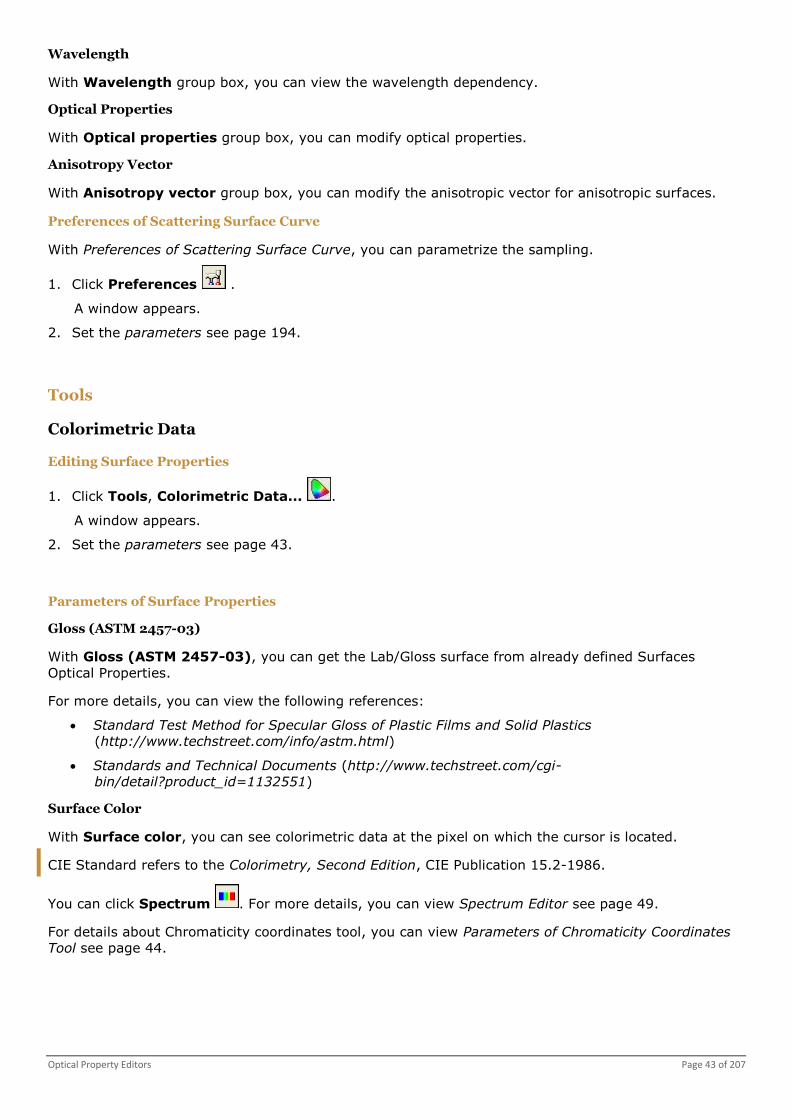
Optical Property Editors Page 43 of 207
Wavelength
With Wavelength group box, you can view the wavelength dependency.
Optical Properties
With Optical properties group box, you can modify optical properties.
Anisotropy Vector
With Anisotropy vector group box, you can modify the anisotropic vector for anisotropic surfaces.
Preferences of Scattering Surface Curve
With Preferences of Scattering Surface Curve, you can parametrize the sampling.
1. Click Preferences .
A window appears.
2. Set the parameters see page 194.
Tools
Colorimetric Data
Editing Surface Properties
1. Click Tools, Colorimetric Data... .
A window appears.
2. Set the parameters see page 43.
Parameters of Surface Properties
Gloss (ASTM 2457-03)
With Gloss (ASTM 2457-03), you can get the Lab/Gloss surface from already defined Surfaces
Optical Properties.
For more details, you can view the following references:
Standard Test Method for Specular Gloss of Plastic Films and Solid Plastics
(http://www.techstreet.com/info/astm.html)
Standards and Technical Documents (http://www.techstreet.com/cgi-
bin/detail?product_id=1132551)
Surface Color
With Surface color, you can see colorimetric data at the pixel on which the cursor is located.
CIE Standard refers to the Colorimetry, Second Edition, CIE Publication 15.2-1986.
You can click Spectrum . For more details, you can view Spectrum Editor see page 49.
For details about Chromaticity coordinates tool, you can view Parameters of Chromaticity Coordinates
Tool see page 44.

Page 44 of 207 OPTIS Labs User Guide
Parameters of Chromaticity Coordinates Tool
With Chromaticity coordinates tool, you can view colorimetric data at the point on which the cursor is
located.
The white curve indicates the color of a black body source in respect of the temperature.
The triangle indicates the domain where your screen displays real color.
With the first list of values, you can choose the units you want in the chromaticity diagram.
The link between xyY and u'v'Y coordinates systems is given by:
u' = 4.x / (-2.x+12.y+3)
v' = 9.y / (-2.x+12.y + 3)
Current Color
On the chromaticity diagram, you can zoom by drawing a rectangle.
You can view the temperature of the color in the status bar.
The temperature is automatically updated when moving the mouse over the map. This temperature
depends of the spectrum.
Ra value is also displayed in the status bar. You must resize the window to see the value. For more
details, you can view Parameters of the Color Rendering Index see page 51.
Reference Color
You can select the Reference color check box to set a reference color and to calculate the DeltaE
between reference color and selected color.
CLS File
By right-clicking on the diagram, you can display contextual menu and choose to display some
information.
By clicking Standard, Select standard..., you can display Colorimetric Standard File (*.cls) box.
By double-clicking on directories, you can select a .cls file.
The definition of a standard is stored in a .cls file. The installation creates some .cls files in
...\OPTIS\Standards\Colorimetry directory.
You can define or add your own standard by adding .cls files into this directory.
You can define the default standard used by Standard, Draw standard. For more details, you can
view Colorimetry see page 195.
CLS File format is the following for a definition with line equations.
Line 1
This is a header line.
OPTIS standard color v1.0
Line 2
This is a comment line as the standard description.
SAE J578 June 27th
Line 3
This line is the definition with line equations.
0
Line 4
This line is the number of areas.
7

Optical Property Editors Page 45 of 207
Line 5
This line is the name of first area.
Selective Yellow
Line 6
The colorimetric diagram is a limit of the area.
1
Line 7
The line is the number of lines without limits given by the colorimetric diagram.
3
Line 8, 9, 10
The lines are operators a and b.
Operators a and b correspond to the line equation y= ax+b.
Operators < and > give the position of the area regarding the line.
Use = for x = constant, for example = 0.5 0 for x=0.5.
> 0.58 0.14
> -1 0.97
>1.29 -0.1
N Lines
Next lines are for the next area as described from lines 5 to 10.
CLS File format is the following for a definition with list of vertexes.
Line 1
This is a header line.
OPTIS standard color v1.0
Line 2
This is a comment line as the standard description.
MIL-S-22885/101C
Line 3
This line is the definition with with list of vertexes.
1
Line 4
This line is the number of areas.
7
Line 5
This line is the name of first area.
Red
Line 6
The colorimetric diagram is a limit of the area.
1
Line 7
The line is the number of vertexes.
4
Line 8
The line is the (x,y) of first vertex.
0.665 0.334

Page 46 of 207 OPTIS Labs User Guide
Line 9
The line is the (x,y) of second vertex.
0.659 0.335
N Lines
Next lines are for the (x,y) of the next vertex and then lines for the next area as described from lines 5
to 9.
Lab/Gloss Surface Definition
With Lab/Gloss Surface Definition you can configure the Lab/Gloss surface which defines the Surfaces
Optical Properties.
Editing Lab/Gloss Surface Properties
1. Click Tools, Lab/Gloss surface definition....
A window appears.
2. Set the parameters see page 46.
Parameters of Lab/Gloss Surface Properties
Gloss
Measurement Angle
In Measurement angle box, you must select 20°, 45° or 60° value.
Gloss Value
In Gloss value box, you must type a Gloss value from 0 to 2030 for measurement angle equal to 20°
and a Gloss value from 1 to 1000 for measurement angle equal to 45° or 60°.
If Gloss value is equal to one thousand, it is a perfect mirror.
Lambertian corresponds to a weak Gloss value.
Two very different surfaces may share the same Gloss value. Gloss value sees them as equivalents
even if they are not.
For more details, you can view the following references:
Standard Test Method for Specular Gloss of Plastic Films and Solid Plastics
(http://www.techstreet.com/info/astm.html)
Standards and Technical Documents (http://www.techstreet.com/cgi-
bin/detail?product_id=1132551)
Gloss value is just one characteristic of the surface, it cannot be used alone to define a surface.
Gaussian Angle (FWHM)
In Gaussian angle (FWHM) box, you must type edit the Gaussian angle value by editing the box,
using the arrows or the blue slider.
FWHM means Full Width at Half Maximum.
FWHM angle is used as following.
For a fixed Gloss value, increasing the Gaussian angle increases the quantity of Gaussian reflected
energy. This may lead to a reflection coefficient higher than one hundred percent.

Optical Property Editors Page 47 of 207
Current Color
In Current color group box, you must type L value.
Maximum value is one hundred.
If L is equal to fifty, it does not mean there will be a 50% Lambertian contribution in the surface.
Details about CIE can be found here (http://www.cie.co.at). Details about Lab color space can be found
here (http://en.wikipedia.org/wiki/Lab_color_space).
When L is equal to one hundred, it is not possible to add further Gloss to surface. The reflection
coefficient would be higher than one hundred percent.
For the same reason, when the Gloss value is one thousand for 45° or 60°, it is not possible to add a
Lambertian contribution using L>0.
It is not possible to generate the surface in case:
The color is outside the screen gamut (the surface state defines its colors in RGB).
The Gloss parameters, the Gaussian angle and the L value generate a reflection coefficient which is
higher than one hundred percent.
For details about Chromaticity coordinates tool, you can view Parameters of Chromaticity Coordinates
Tool see page 44.
Editing the Preferences
1. Click Tools, Preferences... .
A window appears.
2. Set the preferences see page 194.
Autofill
With Autofill, you get some help to generate an Advanced Scattering Surface.
Using Autofill
1. Click Tools, Autofill....
A window appears.
2. Set the parameters see page 47.
3. Click Apply.
Parameters of Autofill
Spectrum import
Filename
You must click Open to select a spectrum.
You can edit the spectrum see page 49 .
Select
You must select a reflection or transmission type.
Wavelength Sampling
You can select Use spectrum sampling check box to use the spectrum sampling.
You can select Use current sampling check box to use the sampling from table included in the main
window.

Page 48 of 207 OPTIS Labs User Guide
Other Properties
You can select Put other value to 0.0 check box to set all other values to zero.
You can select Define value for other properties check box to define values manually.
You can select Keep other value unchanged check box to do not change values from table included in
the main window.
Fresnel Contribution
The Fresnel contribution box calculates the Fresnel reflection coefficient between the air and the
material.
Material Filename
You must click Open to select a material.
Select
You must select a reflection type.
Polarization
You must select Parallel, Undefined or Orthogonal check box to define the polarization type.
Thick Transparent
You can select Thick transparent check box to take into account secondary and more reflections.
Fill Transmission
You can select Fill transmission check box to fill transmission column.
Multiply Lambertian Reflection by Fresnel Transmission
You can select Multiply lambertian reflection by fresnel transmission check box to not to have
negative absorption values when adding a Fresnel contribution.
The lambertian reflection is multiplied by the Fresnel transmission coefficient.
Standard applications are painting and varnish.
Apply a Value to a Selection of Cells
You can select one column, all columns, one row or all rows.
You must select a reflection or transmission type.
You can then apply a value to the specific cell(s).
Others Options
TFCalc Import
TFCalc is only working on 32 bits operating system.
With TFCalc import, you can analyze and design multilayer thin film coatings.
A demo version is given with our software.
A TFCalc coating can be applied on a surface.
1. Set the parameters see page 199.
2. Click File, Import....

Optical Property Editors Page 49 of 207
Auto-calculate Value Option
Using Auto-calculate Value Option
1. Click Options, Auto-calculate value.
2. Set the parameters see page 49.
Parameters of Auto-calculate Value Option
You must select Reflection coefficient, Transmission coefficient or Absorption coefficient to
choose the self-calculating coefficient.
Command formula is A + R + T = 100
Polarization
This polarization option is related to the Coated Surface Editor see page 27.
Using Polarization Option
1. Click Options, Polarization.
2. Set the parameters see page 49.
Parameters of Polarization Option
You must select Force same values for S and P or Allow different values for S and P to force
same value for both polarization or non-polarization.
Spectrum Editor
With Spectrum Editor, you can easily draw the spectrum curve defining particular points.
The editor calculates every point by linear interpolation.
Using the Spectrum Editor
1. From Start menu, click All Programs, OPTIS, OPTIS Labs, Optical Property Editors,
Spectrum Editor.
-Or-
1. Click Spectrum editor .
A window appears.
You can create, open or save a spectrum. In this case you can save your spectrum as a .spectrum
file.
2. Set the parameters see page 50.
You can right click on the spectrum plot to export spectrum data.
You can import measure file.
You can print or copy the spectrum.
You can view colorimetric data see page 44.
You can view Color Rendering Index see page 50.
You can view Lumen-Watt ratio.
You can generate a spectrum see page 52.
You can edit preferences see page 47.

Page 50 of 207 OPTIS Labs User Guide
Parameters of a Spectrum
Value (%)
For each wavelength, you must type a value corresponding to the part of this wavelength power in the
total spectrum power.
If needed, you can Add or Delete a wavelength.
You can add a point by double clicking on the graph.
You can add up to 32767 wavelengths.
If you add too many wavelengths, the displayed spectrum will not be complete.
You must keep in mind that the power of the source is not defined here.
Beware when using spectral maps (illuminance, intensity and luminance) with narrow spectrum
sources (laser, LEDs…).
The default detector wavelength sampling is 13 on a broadband spectrum (from 380 nm to 780 nm).
When using narrow spectrum sources, the detector sampling might not be sufficient and might cause
erroneous results.
This under sampling is also possible when using broadband spectrum with particular peaks as an
example the white LED with blue peak.
Be sure to modify the detector sampling (and/or range) in order to attain a sampling equivalent to the
source spectrum sampling.
The determination of the detector sampling and range must be taken carefully in Indirect simulation or
simulation using fluorescence.
This point is also very important when a very precise colorimetric analysis has to be done.
Absorption Coefficient
Absorption coefficient is used in User Material Editor.
If needed, you can Add or Delete a wavelength.
You can add a point by double clicking on the graph.
Spectrum Format
Line 1
This is a header line.
OPTIS - Spectrum file v1.0
Line 2
This is a comment line as the dye description.
Line 3
This line is the number N of wavelength.
3
N lines
Each line contains a wavelength and the corresponding spectral value.
330 0
380 0.3
600 1.7
Color Rendering Index
The Color Rendering Index is the effect of a light source on the color appearance of objects in
comparison with their color appearance under a reference illuminant for specified conditions.
Color Rendering Index is a colorimetric difference calculated between a luminous source and the
closest black body when you light different colored samplings.

Optical Property Editors Page 51 of 207
Color Rendering Index is available from Virtual Photometric Lab see page 196, Virtual Human Vision
Lab see page 69 and Spectrum Editor see page 49.
Editing the Color Rendering Index Value
You must upload spectral data of xmp first.
The General Color Rendering Index is the average of the first eight Special Color Rendering Index.
From OPTIS Labs 2011 SP1, it is possible to display the Special Color Rendering Index for the fifteen
test samples defined by the CIE.
1. If you have Virtual Photometric Lab or Virtual Human Vision Lab, click Tools, Color
Rendering Index (CRI)....
2. If you have Spectrum Editor, click View, Color Rendering Index (CRI)....
3. If you have Surface / Section window, click .
4. View the parameters see page 51.
5. Close the window.
Parameters of the Color Rendering Index
The first column corresponds to the test sample number.
The third column corresponds to the appearance of the test sample illuminated by the D65 illuminant.
The fourth column shows the color of the sample illuminated by the reference illuminant. This color is
used to calculate the General Color Rendering Index and it changes according to the spectral data.
The fifth column shows the color of the sample illuminated by the present spectrum.
The final column gives the color rendering index of the sample.
The colors are displayed as an indicative way.
Color Rendering Index is also called Ra (Roughness Standard).
Some surfaces from manufacturers like Charmille are described using Ra.
The relation between Ra and Charmille number is the following formula:
N° Ch = 20 log (10 * Ra)
With Ra in micrometers.
Examples
Ra = 1 => N° Ch = 20
Ra = 2 => N° Ch = 26
You can view Ra and Chromaticity Difference (DC) values defined by the CIE.
Details about CIE can be found here
(http://www.cie.co.at/index.php/Publications/index.php?i_ca_id=303).
Ra value is followed by the illuminant reference name used to calculate Ra.
Ra value is also displayed in the status bar of the Colorimetric data diagram. For more details, you can
view Parameters of Chromaticity Coordinates Tool see page 44.
Spectrum Generation
Spectrum Generation is available from Spectrum Editor see page 49.
With Spectrum Generation, you can generate a spectrum corresponding to a black body or a Gaussian
spectrum.

Page 52 of 207 OPTIS Labs User Guide
Generating a Spectrum
1. Click Tools, Spectrum generation... .
2. When the window asks if you want to save the changes, click Yes or No.
A window appears.
3. Set the parameters see page 52.
4. Close the window.
Parameters of Spectrum Generation
You must select Blackbody Spectrum or Gaussian Spectrum.
Blackbody Spectrum
In Temperature box, you must type the temperature in Kelvins.
Gaussian Spectrum
In Center Wavelength box, you must type the center wavelength value in nanometers.
In Diameter at 1/e2 box, you must type the diameter value at 1/e2 in nanometers.
In Lambda Min. box, you must type the minimal lambda value in nanometers.
In Lambda Max. box, you must type the maximal lambda value in nanometers.
In Samples box, you must type the number of samples.
User Material Editor
With User Material Editor, you can build complex materials and store them in a library.
These materials take into account the diffusion, index and absorption variation, gradient index and
birefringent properties.
Using the User Material Editor
1. From Start menu, click All Programs, OPTIS, OPTIS Labs, Optical Property Editors, User
Material Editor.
-Or-
1. Click User Material .
A window appears.
You can create, open or save a material. In this case you can save your material as a .material
file.
2. Set the parameters see page 53.
You can edit material color see page 61.
You can edit preferences see page 63.

Optical Property Editors Page 53 of 207
Parameters of a User Material
General
In Description box, you can type a comment line.
In Material Type box, you must select the material type.
Isotropic
The refractive index is constant in direction but it can vary with the wavelength.
Birefringent
Birefringent material could only be used with optical polished surfaces. Two birefringent materials
cannot be in contact.
For SPEOS Standalone, birefringent materials are only available for BOX, CYLINDER LENS,
POLYHEDRON CSG and BREP (OSB) geometries.
This material has different refractive index associated with different crystallographic direction.
Birefringents materials are defined starting from a 3*3 matrix called dielectric tensor.
There is a reference in which this matrix is diagonal and whose diagonal elements correspond to the
refractive index for different directions of the reference. This reference could be defined in the .geo
file.
In Additional properties box, you must select Uniaxial negative, Uniaxial positive or Biaxial.
In Vector I and Vector J boxes, you must set coordinate values for Vector I and Vector J.
The reference in which the matrix is diagonal is the same one that the global reference.
Dielectric tensor sample
Gradient Index
The refractive index varies as a function of the location in the material.

Page 54 of 207 OPTIS Labs User Guide
Refractive index varies as a function of radius as defined by the displayed formula.
n0 is defined by the index variation.
The r distance is measured compared to a reference axis as shown on the diagram. This axis passes by
the origin of the object.
Sample with A=0.499, n0 = 1.564 at 632 nm
Gradient index materials are only available for BOX and CYLINDER CSG geometries.
Gradient Index and Birefringent Examples
These examples are only with SPEOS Standalone and OptisWorks software.
There are 2 additional parameters in the geo script for gradient index and birefringent materials.
MATERIAL_VECTOR_I
MATERIAL_VECTOR_I is only used when the object is made of birefringent or gradient index material.
With MATERIAL_VECTOR_I, you can define the reference axis for a gradient index material.
Vector's coordinates are given in the local referential.
For Birefringent material, you can define the first axis of the referential in which the dielectric tensor is
diagonal. In this case coordinates of the axis are given in the global referential.
MATERIAL_VECTOR_J
MATERIAL_VECTOR_J is only for birefringent material.
With MATERIAL_VECTOR_J, you can define the second axis of the referential in which the dielectric
tensor is diagonal. It has to be orthogonal to MATERIAL_VECTOR_I.
The same material can be applied to several objects and it must have for each object a different
referential.
For birefringent materials, MATERIAL_VECTOR_I and MATERIAL_VECTOR_J are optional in the geo
script.
If they are not defined in the geo script, the default axes defined with the editor and saved within the
material file will be used.
In OptisWorks software, birefringent material is oriented by the part preferences.
Fluorescent
The material includes fluorescent dyes.

Optical Property Editors Page 55 of 207
The fluorescent material usage is the same as any other material. The only difference is that you can
enter fluorescence specific data as absorption spectrum, re-emission spectrum, quantum efficiency,
measure concentration and user concentration.
In Fluorescent tab, you can Add or Delete pigment.
You can click to edit measured or user concentration.
Measured concentration is the dye concentration when the fluorescent dye has been measured.
User concentration is the concentration defined by the user for simulations.
Concentration unit has to be the same for both concentrations. As a reminder you can type the used
unit in the comment line of the dye.
You can double click on dye to edit pigment properties. For more details, you can view Dye Editor see
page 59.
Metallic
The metallic material correctly interacts with polarized light. Since the polarization is taken into
account, the material's reflectance changes when the incidence angle varies.
When you apply this material to a part, the reflection automatically takes the effects due to
polarization into account.
It is not the energy penetrating the material which is calculated here, but only the reflected energy.
The metallic material type cannot be used to model thin metallic coats.
Index Variation
For Isotropic, Gradient Index or Fluorescent material, you must select the model used to
describe the index variation. This can be by giving index in function of wavelength, using the
SellMeier formula, using the Kettler-Helmholtz formula or index and constringence.
For Birefringent material, you must select the model used to describe the index variation. This
can be constant index, using the SellMeier formula or using the Kettler-Helmotz formula.
Uniaxial positive material is when na=nb < nc, na and nb are ordinary index.
Uniaxial negative material is when na<nb=nc, nb et nc are ordinary index.
Biaxial material is when na # nb # nc.
na, nb,nc are the refractive index for the referential in which the dielectric tensor is diagonal.
You must have na < nb < nc.
For Metallic material, you cannot use a model to describe the index variation in function of
wavelength. You must set the index values directly in the table.
The Index variation is here composed of two parts : the real part and the imaginary part. This is
because, for a metallic material, the index of refraction is a complex number composed of a real
part and of an imaginary part.
The index of refraction corresponds to n-i*k, n being the real part and k the imaginary part.
You can select the Real and Imaginary check boxes in Spectrum to respectively display real and
imaginary parts' spectra.
If needed, you can Add or Delete a column.
Absorption Variation
The concentration parameters are used when the absorption is due to a pigment diluted in a main
material, typically a colored plastic.
Measured Concentration
When you measure the optical absorption of a plastic that has a known pigment concentration also
called Measured concentration, you put this absorption in the material absorption table.

Page 56 of 207 OPTIS Labs User Guide
User Concentration
The User concentration is the pigment concentration used for the simulation.
If the user concentration is the same as the measured concentration, then you are simulating using
exactly the plastic you measured.
You have the possibility to do a simulation with a plastic that has a different pigment concentration
without having to create and measure a new piece of plastic. You have to put the new concentration in
the User concentration box. You are now ready to simulate. The software computes the new
absorption from the absorption spectrum, the measure concentration and the user concentration.
If needed, you can Add or Delete a column.
Scattering Properties
You can define the volume scattering (material like fog).
In General group box, you must select scattering variation model.
Unscattering Material
If you select Unscattering material, the material does not include scattering variation.
Give Particles Specifications: Optical Properties of the Medium will be Evaluated using MIE Theory
If you select Give particles specifications: Optical properties of the medium will be evaluated
using MIE theory, the scattering variation is described by a table of diffusion coefficients (mm-1) for
each wavelength (nm) corresponding to the list of particles.
With the scattering variation tab, you can describe the scattering efficiency according to the scattering
angle.
Transmission = exp (- diffusion coefficient * thickness)
This model is used to describe volume scattering material with small particles. With the material editor,
you can define the size, the index and the density of the particles.
Particles tab is available. For more details, you can view Particles see page 59.
Scattering variation and Scattering phase function tabs are automatically computed and updated.
Scattering phase function tab cannot be modified. For more details, you can view Scattering Phase
Function see page 58.
Give Scattering Coefficient and Phase Function of the Medium
If you select Give scattering coefficient and phase function of the medium, the scattering
variation is described by a table of diffusion coefficients (mm-1) for each wavelength (nm) and by a
phase function.
With Scattering variation tab, you can describe the scattering efficiency according to the scattering
angle.
Transmission = exp (- diffusion coefficient * thickness)
You must then select if phase function is defined by giving scattering efficiency according to the
scattering angle, by using Henyey-Greenstein formula or by using a double Henyey-Greenstein
formula.
Henyey-Greenstein
Henyey-Greenstein model simplifies the phase function's definition for the intensity distribution. With
this model, you have to give the anisotropic factor to describe the intensity distribution. This data can
be found in data sheet.
All the difficulty in diffusing material coding is in the appropriate choice of phase function to be as
closer as possible to physical laws.

Optical Property Editors Page 57 of 207
Jacques and Prahl [S. L. Jacques, C. A. Alter, and S. A. Prahl. Angular dependence of HeNe laser light
scattering by human dermis. Lasers Life Sci., 1:309{333, 1987.] have shown that the following phase
function is very appropriate to simulate human skin.
Theta is the angle between and .
G = 0 G = 0.8
Double Henyey-Greenstein
Double Henyey-Greenstein model is for diffuse material in volume.
The Double Henyey-Greenstein model formula is the following:
F(Theta)= Ratio*f(Theta, Anisotropy factor1)+ (1-Ratio)*f(theta, Anisotropy factor 2)
For details about Scattering phase function tab, you can view Scattering Phase Function see page
58.
Phase Function Changes According to the Wavelength
In case of MIE theory, if you select the Phase function changes according to the wavelength
check box, you first need to add one particle. For more details, you can view Particles see page 59.
In case of Give scattering coefficient and phase function of the medium, if you select the Phase
function changes according to the wavelength check box, you can Add or Delete a
wavelength and/or an angle.
The wavelength list is the same than the one displayed in the Scattering variation tab. If you want to
add a wavelength to the phase table, you can do it from Scattering variation tab.
With Wavelength to display, you can select the wavelength of the table for which the phase
function's display has been made.

Page 58 of 207 OPTIS Labs User Guide
Scattering Phase Function
Phase Function Definition
Volumic diffusion is a physical process which occurs when a particle of material absorbs some energy
of an incident electromagnetic wave, in the direction of propagation.
This energy is then redistributed around this particle according to a specific angular function which is
called phase function.
This function has many parameters as the particle's size, wavelength, and the material and particle
indexes.
According of Monte-Carlo propagation, this phase function can be assimilated to a probability for a
photon which is propagated in direction to be diffused in direction.
This function is named .
You can normalize this function with:
The following phase function corresponds to an isotropic diffusion:
Anisotropy Factor
Anisotropy factor is available when Give scattering coefficient and phase function of the
medium: Define phase function using Henyey-Greenstein formula, or Define phase function
using a double Henyey-Greenstein formula is selected.
When the phase function is not isotropic, you must characterize isotropy with g parameter called
Anisotropy factor with following definition:
When g is converging to 1, the diffused electromagnetic energy is very near initial propagation
direction.
On the other side, when g is equal to 0 you get back an isotropic diffusion and when g is negative you
get retro diffusion properties.
Display
By selecting the View shading check box, you can display a shading view of the intensity
envelope.
By selecting the View Mesh check box, you can display the intensity envelope with wireframe.
By selecting the Decorations check box, you can display the 3D view tool.
For more details, you can view Using 3D view tool.
By selecting the Axis System check box, you can display the axis system.
You can edit 3D view preferences. For more details, you can view 3D View see page 196.
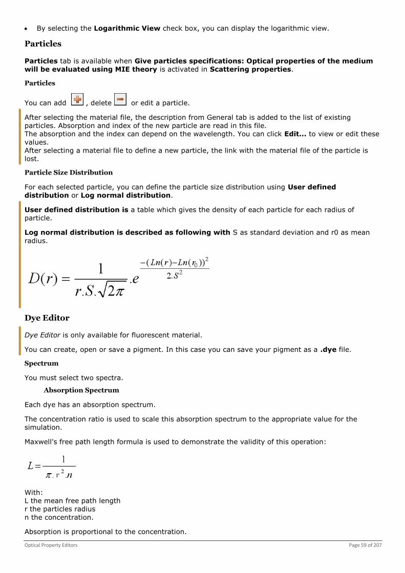
Optical Property Editors Page 59 of 207
By selecting the Logarithmic View check box, you can display the logarithmic view.
Particles
Particles tab is available when Give particles specifications: Optical properties of the medium
will be evaluated using MIE theory is activated in Scattering properties.
Particles
You can add , delete or edit a particle.
After selecting the material file, the description from General tab is added to the list of existing
particles. Absorption and index of the new particle are read in this file.
The absorption and the index can depend on the wavelength. You can click Edit... to view or edit these
values.
After selecting a material file to define a new particle, the link with the material file of the particle is
lost.
Particle Size Distribution
For each selected particle, you can define the particle size distribution using User defined
distribution or Log normal distribution.
User defined distribution is a table which gives the density of each particle for each radius of
particle.
Log normal distribution is described as following with S as standard deviation and r0 as mean
radius.
Dye Editor
Dye Editor is only available for fluorescent material.
You can create, open or save a pigment. In this case you can save your pigment as a .dye file.
Spectrum
You must select two spectra.
Absorption Spectrum
Each dye has an absorption spectrum.
The concentration ratio is used to scale this absorption spectrum to the appropriate value for the
simulation.
Maxwell's free path length formula is used to demonstrate the validity of this operation:
With:
L the mean free path length
r the particles radius
n the concentration.
Absorption is proportional to the concentration.

Page 60 of 207 OPTIS Labs User Guide
When propagating a photon, we compute a random distance according to the dye's absorption.
Then the photon has a probability equal to the quantum efficiency to be re-emitted with a new
wavelength.
This new wavelength is chosen randomly using the dye's emission spectrum.
Finally, we compute a new random direction for the photon.
Note that for the computation the photon's direction generated by florescence does not depend on the
photon's direction which has been absorbed. It is emitted again in an isotrope way, all directions are
equiprobable.
Then we propagate the photon to the next interaction.
Absorption spectrum has to be defined in mm-1.
You can click Spectrum to edit a spectrum or browse an existing spectrum. For more details, you
can view Spectrum Editor see page 49.
Efficiency Spectrum
The efficiency value is spectral. The related spectrum has to be written in percentage.
You can click Spectrum to edit a spectrum or browse an existing spectrum. For more details, you
can view Spectrum Editor see page 49.
Excitance Spectrum
Excitance spectrum is obtained by multiplying the absorption spectrum by the efficiency spectrum.
You can click Spectrum to edit a spectrum or browse an existing spectrum. For more details, you
can view Spectrum Editor see page 49.
Emission Spectrum
You can click Spectrum to edit a spectrum or browse an existing spectrum. For more details, you
can view Spectrum Editor see page 49.
Scattering Properties
For more details, you can view Scattering properties see page 56.
Particle: Refractive Index and Size
Particle: refractive index and size is available when Give particles specifications: Optical
properties of the medium will be evaluated using MIE theory from Scattering properties tab
has been selected.
With Particle: refractive index and size tab, you can select a .material file containing the pigment
refraction index. In this case the material absorption, diffusion and fluorescence parameters are not
taking into account.
Emission Distribution Type
Emission distribution type tab is available when Unscattering material from Scattering
properties tab has not been selected.
You can select the Emission distribution changes according to the wavelength check box to
define an emission function by wavelength.
When no selecting Isotropic emission distribution, you can edit the Emission distribution.
Theta is the angle between the incident photon angle on the pigment and the direction of the photon
emitted by pigment's fluorescence.

Optical Property Editors Page 61 of 207
Material Color
Editing Material Color
With Material Color, you can display the resulting color if the light comes from a black body (3200°K)
through 1 mm, or the material preview of the material color giving the light source's spectrum and
material thickness.
1. Click Tools, Colorimetric Data... .
A window appears.
2. Set the parameters see page 61.
Parameters of Material Color
Light Source
In Light Source group box, you can select User Spectrum or Blackbody spectrum.
If selecting User Spectrum, you must browse a spectrum file.
You can click Edit to edit the spectrum file. For more details, you can view Spectrum Editor see page
49.
If selecting Blackbody spectrum, you can change the temperature in Kelvin.
Material Thickness
In Material Thickness group box, you must set the material thickness value in millimeters.
For details about Chromaticity coordinates tool, you can view Parameters of Chromaticity Coordinates
Tool see page 44.
Parameters of Chromaticity Coordinates Tool
With Chromaticity coordinates tool, you can view colorimetric data at the point on which the cursor is
located.
The white curve indicates the color of a black body source in respect of the temperature.
The triangle indicates the domain where your screen displays real color.
With the first list of values, you can choose the units you want in the chromaticity diagram.
The link between xyY and u'v'Y coordinates systems is given by:
u' = 4.x / (-2.x+12.y+3)
v' = 9.y / (-2.x+12.y + 3)
Current Color
On the chromaticity diagram, you can zoom by drawing a rectangle.
You can view the temperature of the color in the status bar.
The temperature is automatically updated when moving the mouse over the map. This temperature
depends of the spectrum.
Ra value is also displayed in the status bar. You must resize the window to see the value. For more
details, you can view Parameters of the Color Rendering Index see page 51.
Reference Color
You can select the Reference color check box to set a reference color and to calculate the DeltaE
between reference color and selected color.
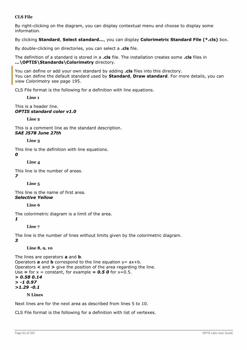
Page 62 of 207 OPTIS Labs User Guide
CLS File
By right-clicking on the diagram, you can display contextual menu and choose to display some
information.
By clicking Standard, Select standard..., you can display Colorimetric Standard File (*.cls) box.
By double-clicking on directories, you can select a .cls file.
The definition of a standard is stored in a .cls file. The installation creates some .cls files in
...\OPTIS\Standards\Colorimetry directory.
You can define or add your own standard by adding .cls files into this directory.
You can define the default standard used by Standard, Draw standard. For more details, you can
view Colorimetry see page 195.
CLS File format is the following for a definition with line equations.
Line 1
This is a header line.
OPTIS standard color v1.0
Line 2
This is a comment line as the standard description.
SAE J578 June 27th
Line 3
This line is the definition with line equations.
0
Line 4
This line is the number of areas.
7
Line 5
This line is the name of first area.
Selective Yellow
Line 6
The colorimetric diagram is a limit of the area.
1
Line 7
The line is the number of lines without limits given by the colorimetric diagram.
3
Line 8, 9, 10
The lines are operators a and b.
Operators a and b correspond to the line equation y= ax+b.
Operators < and > give the position of the area regarding the line.
Use = for x = constant, for example = 0.5 0 for x=0.5.
> 0.58 0.14
> -1 0.97
>1.29 -0.1
N Lines
Next lines are for the next area as described from lines 5 to 10.
CLS File format is the following for a definition with list of vertexes.

Optical Property Editors Page 63 of 207
Line 1
This is a header line.
OPTIS standard color v1.0
Line 2
This is a comment line as the standard description.
MIL-S-22885/101C
Line 3
This line is the definition with with list of vertexes.
1
Line 4
This line is the number of areas.
7
Line 5
This line is the name of first area.
Red
Line 6
The colorimetric diagram is a limit of the area.
1
Line 7
The line is the number of vertexes.
4
Line 8
The line is the (x,y) of first vertex.
0.665 0.334
Line 9
The line is the (x,y) of second vertex.
0.659 0.335
N Lines
Next lines are for the (x,y) of the next vertex and then lines for the next area as described from lines 5
to 9.
Editing the Preferences
1. Click Tools, Preferences... .
A window appears.
2. Set the preferences see page 194.

Page 64 of 207 OPTIS Labs User Guide
LABS
Photometric Calc
With Photometric Calc, you can make operations on map.
Using Photometric Calc
1. From Start menu, click All Programs, OPTIS, OPTIS Labs, Labs, Photometric Calc.
-Or-
1. Click Photometric Calc .
A window appears.
2. Set the parameters see page 64.
3. Click Close.
Parameters of Photometric Calc
Source Files
In Source Files group box, you have to select one or two maps depending on the type of operation.
In Operation box, you must select the operations in the operation list.
MAP ADDITION map1 + map2
MAP SUBTRACTION map1 - map2
VALUE MULTIPLICATION map1 * value
MAP MULTIPLICATION map1 * map2
MAP DIVISION map1 / map2
This operation does not work with spectral maps.
VERTICAL AXIS SYMMETRY This operation makes a vertical axis symmetry on the data of
map1.
HORIZONTAL AXIS SYMMETRY This operation makes an horizontal axis symmetry on the data of
map1.
VERTICAL AXIS MIRROR This operation makes a vertical mirror on the data of map1.
HORIZONTAL AXIS MIRROR This operation makes an horizontal mirror on the data of map1.
ROTATION This operation rotates map1 with an angle.
You must type the angle value in degrees.
MERGE RESULTS This operation makes an addition of map1 and map2 taking into
account number of integrated rays of each one.
It is possible to merge xmp spectral maps which do not have
same wavelength sampling, only in case spectral data are not
saved in the XMP. If the sampling is not the same and spectral
data are saved, you can read a message suggesting to export the
XMP without spectral data.
MAP UNION (COMBINE TWO MAPS IN ONE)
This operation creates a spectral or an extended map with N1+N2
layers.
N1 is the number of layers of map1.
N2 is the number of layers of map2.
SPECTRUM MULTIPLICATION This operation makes the multiplication of a basic or a spectral

Labs Page 65 of 207
MAP ADDITION map1 + map2
map by a .spectrum file.
SIGNAL TO NOISE RATIO The division is not made source by source but on the complete
map with the possibility to visualize the contribution to the signal
to noise ratio from each source. Signal Noise Ratio = Luminance
map1/Luminance map2.
This operation works with basic, extended and spectral maps.
ABSOLUTE VALUE
Operations are available on all types of maps.
Result
In Result box, you have to select one map for result.
Virtual 3D Photometric Lab
With Virtual 3D Photometric Lab, you can view photometric or radiometric information as reflection,
transmission, absorption or irradiance directly on your 3D model.
Using Virtual 3D Photometric Lab
1. From Start menu, click All Programs, OPTIS, OPTIS Labs, Labs, Virtual 3D Photometric Lab.
-Or-
1. Click Virtual 3D Photometric Lab .
A window appears.
2. Click File, Open ....
-Or
Click .
3. Select a SPEOS 3D map file.
SPEOS 3D map file is a .xm3 format.
You can save a 3D map file. In this case you can save your 3D map as a .xm3 file.
By clicking , you can export a 3D map in a .txt file format. You can then open it with Excel
software and find hot spots.
This .txt file includes x, y, z coordinates of each vertex, value of each layer (Transmission,
Reflection...) and for 3D map including color, the X, Y and Z colorimetric coordinates.
You can click File, Info to get file information as number of nodes, number of cells, generated
photons, emitted photons, absorbed photons, radiometric or photometric power.
You can click to choose color level display.
You can manage display see page 66.
You can do post-processing see page 66.
You can make surface and section analysis see page 67.
You can edit preferences see page 69.
By clicking Filtering, XM3 Filtering..., you can set a standard filtering.
It only uses neighbors without any considerations regarding values of these neighbors.
In Pass number box, you must type the number of times the filtering algorithm is called. 0 value
means there is no filtering.

Page 66 of 207 OPTIS Labs User Guide
The level of filtering is displayed in the status bar of the viewer. By clicking the filter value in the
status bar, you can open the filtering box.
Managing the Display
Display
By selecting the Decorations check box, you can display the 3D view tool.
For more details, you can view Using 3D view tool.
By selecting the View Mesh check box, you can display the intensity envelope with wireframe.
By selecting the Mesh limit check box, you can display the mesh limit.
By selecting the Legend check box, you can display the legend.
By selecting the Axis check box, you can display the axis.
By selecting the Clip plane check box, you can display the clip plane.
By selecting the Contour check box, you can display the contour.
You can select the Colored check box to color contour.
You can select the Annotation check box to display value of each contour line.
You can select a value in the both level lists.
Transparent
In Transparent box, you can move the slider to set the transparency.
In Max and Min boxes, you can change the maximal and minimal level of colors on the map.
By clicking Default values, you can save values as default values.
3D Map Post-Processing
Doing 3D Map Post-Processing
With 3D map Post-Processing, you can compute illuminance or luminance directly on a 3D geometry.
You must have opened a 3D map resulting from a direct simulation.
Illuminance post-processing gives same result than standard simulation result except that it can be
displayed in false or true color.
Luminance post-processing gives same result than a 2D XMP map luminance post-processing except
that result is in 3D instead of 2D. This avoids blurred results on curved geometry.
1. Click Post-processing, Irradiance/Illuminance from ray file....
-Or-
1. Click Post-processing, Radiance/Luminance from ray file....
A box appears.
2. Set the parameters see page 67.
3. Click to launch the post-processing.
A progress bar appears.
An illuminance or luminance 3D map appears.
If you want to select a false or true color display, use the color list.
If you want to change the unit display, use the unit list. Radiometric unit is displayed in W/(m².sr),
and photometric unit in cd/m².

Labs Page 67 of 207
Parameters of 3D Map Post-Processing
Initial Ray File
In File box, you must click and browse a .ray file.
You can read Ray file size, Radiant flux, Ray file data and Number of rays values.
If needed, you can select the Luminous flux check box to display the luminous flux value in lumens.
Parameter
In Wavelength group box, you can change Wavelength parameters.
In Wmin box, you can type the minimal wavelength value in nanometers.
In Wmax box, you can type the maximal wavelength value in nanometers.
In Nb W box, you can type the number of wavelength.
For luminance post-processing, in Integration angle box you can change the value.
Surface and Section Analysis
Making Surface and Section Analysis
With Surface and Section Analysis tool, you can use the 3D axis to make measurements.
1. Click Tools, Surface...
A box appears and axis appear on your map.
2. Set the parameters see page 67.
Close the window.
Parameters of Surface and Section Analysis
Units are automatically set depending on the type of map (luminance, illuminance...).
If needed, you can use the mouse to change values.
Shape
You must select a type of shape as Rectangle or Ellipse to define the analysis surface.
Center
In Center group box, you must type values to define the position of the object which is the
intersection of the three axes.
Direction
In Direction group box, you must type values to define the direction of the analysis surface.
The direction is from the blue cube toward the center of the object.
Phi is the available rotation at 360 degrees around the blue axis.
Dimension
In Dimension group box, you must type values to define the dimension of the analysis surface.
Section
You can select User line to enable the analysis section.
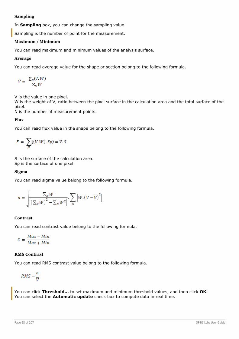
Page 68 of 207 OPTIS Labs User Guide
Sampling
In Sampling box, you can change the sampling value.
Sampling is the number of point for the measurement.
Maximum / Minimum
You can read maximum and minimum values of the analysis surface.
Average
You can read average value for the shape or section belong to the following formula.
V is the value in one pixel.
W is the weight of V, ratio between the pixel surface in the calculation area and the total surface of the
pixel.
N is the number of measurement points.
Flux
You can read flux value in the shape belong to the following formula.
S is the surface of the calculation area.
Sp is the surface of one pixel.
Sigma
You can read sigma value belong to the following formula.
Contrast
You can read contrast value belong to the following formula.
RMS Contrast
You can read RMS contrast value belong to the following formula.
You can click Threshold... to set maximum and minimum threshold values, and then click OK.
You can select the Automatic update check box to compute data in real time.

Labs Page 69 of 207
Editing the Preferences
1. Click Tools, Preferences... .
A window appears.
2. Set the preferences see page 194.
Virtual Human Vision Lab
The human eye has a great dynamic to detect levels of luminance going from 10-6 cd/m² to 108 cd/m².
Unfortunately most of media used to display luminance map obtained using OPTIS software do not
have such a dynamic. As an example, a monitor has a dynamic lower than one hundred.
With Virtual Human Vision Lab, you can reproduce visual appearance of modeled scenes on this media.
Virtual Human Vision Lab restores contrasts perceived by an observer placed in the scene.
All luminance map fields having luminance lower than the detection threshold of the human eye are
not displayed.
This threshold depends on the luminance to which the eye is adapted. It takes into account properties
of the various eye photoreceptors.
Those can be classified in two families:
The first one is called cone and intervenes in the process of colors perception.
The second called rod is much more sensitive and with it you can perceive luminance lower than
0.001 cd/m² for which cone sensitivity is insignificant.
Under this condition, this is the case of a scotopic vision for which you do not have colors
perception.
When luminance becomes higher than approximately 5 cd/m², the rods are subjected to a
phenomenon of saturation. This vision only results in the cones and is called the photopic vision.
When the luminance of adaptation is between 0.005 cd/m² and 5 cd/m², cones and rods intervene
in the vision process. One is then in mesopic vision.
In order to restore the perception of contrasts as well as possible, Virtual Human Vision Lab takes into
account the luminance of the used screen to display the luminance map.
White Point Luminance value has to be the maximum luminance of a white zone displayed by the
used screen. For more details, you can view Monitor see page 194.
Using Virtual Human Vision Lab
1. From Start menu, click All Programs, OPTIS, OPTIS Labs, Labs, Virtual Human Vision Lab.
-Or-
1. Click Virtual Human Vision Lab .
A window appears.
2. Click File, Open ....
-Or-
Click .
3. Browse a .xmp file.
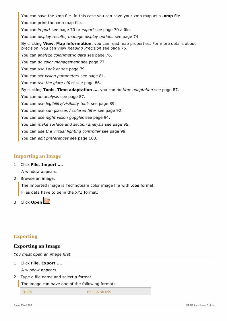
Page 70 of 207 OPTIS Labs User Guide
You can save the xmp file. In this case you can save your xmp map as a .xmp file.
You can print the xmp map file.
You can import see page 70 or export see page 70 a file.
You can display results, manage display options see page 74.
By clicking View, Map information, you can read map properties. For more details about
precision, you can view Reading Precision see page 76.
You can analyze colorimetric data see page 76.
You can do color management see page 77.
You can use Look at see page 79.
You can set vision parameters see page 81.
You can use the glare effect see page 86.
By clicking Tools, Time adaptation ..., you can do time adaptation see page 87.
You can do analysis see page 87.
You can use legibility/visibility tools see page 89.
You can use sun glasses / colored filter see page 92.
You can use night vision goggles see page 94.
You can make surface and section analysis see page 95.
You can use the virtual lighting controller see page 98.
You can edit preferences see page 100.
Importing an Image
1. Click File, Import ....
A window appears.
2. Browse an image.
The imported image is Technoteam color image file with .cos format.
Files data have to be in the XYZ format.
3. Click Open .
Exporting
Exporting an Image
You must open an image first.
1. Click File, Export ....
A window appears.
2. Type a file name and select a format.
The image can have one of the following formats.
FILES EXTENSIONS

Labs Page 71 of 207
FILES EXTENSIONS
XMP map .xmp
Bitmap .bmp
JPeg .jpg
PNG .png
Tiff .tiff
OpenEXR .exr
RGBE .hdr
For more details about .hdr files, you can view HDRI File Format see page 71.
OpenEXR and RGBE are only enable in case of spectral maps.
3. Click Save .
4. In case of a .xmp file export, a box appears. Set the parameters see page 74 and click OK.
HDRI File Format
High Dynamic Range Image (HDRI) is a generic name for an image format which improve the classical
bitmap representation.
Classical bitmaps are coding RGB colors using three 8bits or 16bits integer values (.bmp, .jpg, .tiff...).
The dynamic range of the picture is much more limited than what the eye is able to see in the real
world.
HDRI enables to overcome this problem by using a much wider dynamic range.
Moreover, the color quantization steps are smaller with HDRI. This provides a better colorimetric
accuracy especially when using a wide gamut.
When exporting or importing HDRI for bitmap emission with a better dynamic range, you can not only
simulate displays but also real background illumination.
Today, HDRI are supported by most rendering programs to export the rendering results but also to
import environment map. Environment maps enable to achieve very realistic illuminations. OPTIS
software are able to use environment maps (cube or sphere HDRI maps) to achieve comparable result
and even better result thanks to its physics based calculation.
You can generate good environment HDRI maps using digital cameras and a software tool like
HDRShop.
Supported Formats
RGBE and OpenEXR are supported formats.
RGBE is the native Radiance format. This is the most wide used format today.
ILM 's OpenEXR is the most powerful format to date.
XMPs are even better than HDRI, including spectral data, source separation...
When exporting XMP to HDRI your are able to address the full dynamic provided by HDRI which is not
possible when exporting a BMP to HDRI with a classical rendering software.
XMP export to HDRI: 16 bits to 16 bits
BMP export to HDRI: 8 bits to 16 bits

Page 72 of 207 OPTIS Labs User Guide
HDRI/Classical Bitmap Comparison
Here is a picture having levels divided by two at each step from the left to the right.
Only the left most columns are visible, the other are too dark to be seen. To see the rest of the picture,
one has to saturate the visible part by changing the exposure.
Let us compare what happen if the picture is HDRI (on the right) and if the picture is a classical bitmap
(on the left).
When the exposition increases only slightly, no difference is noticeable
Both formats still look the same

Labs Page 73 of 207
The classical bitmap starts to show its limits
The difference is clear now
The HDRI is able to display the entire picture
As the classical bitmap only has 256 grey levels, all levels inferior to the darker possible grey level are
coded black. This is why they are unrecoverable.
XMP Emission
Now if we compare XMP emission, the XMP is seen through a transparent sphere.
The same simulation was achieved using a HDRI import generated XMP (left column) and a classical
bitmap import generated XMP (right column).
The Virtual Photometric Lab level indicates the light level that is displayed saturated.

Page 74 of 207 OPTIS Labs User Guide
Virtual Photometric Lab level = 2 500 cd/m²
Virtual Photometric Lab level = 10 000 cd/m²
Parameters of XMP Export
The xmp Export is like a Save As except that the export includes options.
These options help to reduce the file's size on the disk.
If you do not need to analyze the spectrum on each pixel of the map and if you do not need to
analyze the data for each wavelength, you can select Include spectral data check box.
If you want to group some sources data of the map, you can select Merge active layer(s) check
box.
If you want to have filtered or original data in the exported file, you can select Export filtered
data check box.
If you want to export a spectral map to convert it into an extended map, you can select
Conversion to extended map check box.
You can select Intensity normalized as luminance check box and set a value for the Surface
box in square millimeters.
Managing the Display
All display's options as filtering level, Surface/Section parameters or layers' configurations are saved
within the Virtual Human Vision map when saving the file.
If you want to move the map, left-click and move the mouse at the same time.
If you want to use the zoom, rotate the IntelliMouse wheel, click Edit, Activate Zoom or click
and then left-click or right-click.
Click to display the original size.
When moving the mouse over the map, values at the position are displayed in the status bar.
The displayed value is interpolated with the value of many pixels. By clicking View, Interpolate
values, you can activate or deactivate the interpolation.
If you want to view spectrum curve at the mouse position, click .
Status bar provides Angle, Depth, Luminance or Relative brightness, Vision Mode, Filter
values.
Angle is the angle between fixation point and the map field pointed by mouse.

Labs Page 75 of 207
Depth is the distance between the observer and the 3D scenery's point pointed by mouse.
Vision Mode can be Photopic, Mesopic or Scotopic. It is estimated to starting from the values of
the displayed luminance map.
Images below show the results when one changes the level of luminance of a simulation of a set of
colored translucent plastics.
With Virtual Photometric Lab
Maximum luminance of the map: 0.7 cd/m²
With Virtual Human Vision Lab, mesopic
vision
Maximum luminance of the map: 0.7 cd/m²
Following images were obtained with Photometric Calc by multiplying luminance value of the initial
map.
In case of scotopic vision, there is a very poor colors perception because cone sensitivity is
insignificant. Cones are responsible of color perception.
In case of mesopic vision, as the map luminance increases, one starts to perceive some colors:
first red color, then orange, green and last blue.
With Virtual Human Vision Lab, mesopic
vision
Maximum luminance of the map: 0.35 cd/m²
With Virtual Human Vision Lab, scotopic vision
Maximum luminance of the map: 0.005 cd/m²
If you want to modify the number format, right-click on the status bar.
The number format is the number of decimal per value.
If you want to switch between luminance unit and relative brightness, click View, Relative
brightness.
Brightness is a subjective attribute of light to which humans assign a label between very dim and
very bright.
Brightness is perceived but not measured.
The sensitivity of the eye to luminance is non-linear and complex that's why brightness notion is
used.

Page 76 of 207 OPTIS Labs User Guide
The most brilliant point of the map has a relative brightness of 100.
If you want to modify the axis unit of displayed values, right-click on the status bar.
If you want to display grids and other options, right-click on the map to select tools.
As an example you can show ruler, set ruler parameters, show axis on cross, snap cross to grid,
show tooltip, show gray around the map, fill shape, show primary or secondary graduations, set
graduations parameters, show primary or secondary grids, set grid parameters.
Reading Precision
Precision Value
In direct simulation, the displayed precision value corresponds to the pixel having the highest number
of integrated rays.
Precision formula is the following.
Precision = 1/sqrt(N)
With N the number of rays integrated by the pixel.
When no rays are integrated on a pixel, the error is infinite. The precision value is one hundred
percent.
In direct simulation using radiance luminance sensor with activated gathering, precision does not have
any meaning. Precision value is also one hundred percent.
In inverse simulation using the Monte-Carlo algorithm, a number of pass has to be specified as 100
passes = 100 rays per pixel (not necessary effective rays).
Precision formula is the following.
Precision = 1/sqrt(N)
With N the number of passes.
In inverse simulation using determinist or photon map algorithms, precision does not have any
meaning. Precision value is also one hundred percent.
Higher is the precision percent, lower is the image quality.
Be aware that one pixel which has not received any rays or which has received only one has a one
hundred percent precision.
More rays or passes there are, lower is the statistical noise. A direct correlation between this number
and the error (or variance, standard deviation) is not possible.
For systems under weighted Monte-Carlo algorithms, the only way to compute error (variance) is to
launch the same simulation several times and to calculate the standard deviation of specific pixels.
The statistical error is always less important for pixels with more integrated rays.
Precision Map
For direct simulation, you can click Tools, Precision map... to display the precision map.
The precision map is only validate for all sources set at one hundred percent when there is no any
separation by sources.
The precision is displayed in percent and is saved in rays number in the map. You can then generate
precision calculation with the surface / section analysis tool.
Analyzing Colorimetric Data
Three tools are available to analyze colorimetric data.
Labs Page 77 of 207
If you want to see colorimetric data at a specific pixel location, you can click Tools, Colorimetric
data... or .
For more details, you can view Parameters of Chromaticity Coordinates Tool see page 44.
If you want to analyze the error between the color displayed by the screen and the reality for all
points of the map, you can click Tools, Colorimetric error....
The true color luminance map is replaced by a colorimetric error map displayed in false color.
When the dynamic of the luminance map is higher than the one of the screen, the Lab compresses
the luminance using a linear relation.
With colorimetric error tool, you can analyze the error between the color after compression and the
color really displayed by the screen.
The colorimetric error is calculated using the CIE94 (1 :1 :1) formula (CIE 116-1995).
When the dynamic of the luminance map is lower than the one of the display, there is no
luminance compression. In this case the displayed error is the one between the color contained in
the luminance map and the one really displayed.
If you want to have all information about the spectrum for all points of the map, you can click
Tools, Spectrum... or .
For more details, you can view Spectrum Editor see page 49.
If you want to read the color rendering index values, you can click Tools, Color Rendering Index
(CRI) ....
For more details, you can view Parameters of the Color Rendering Index see page 51.
Doing Color Management
A number of color are physically not reproducible by a display.
We say that colors are outside of the gamut of the display.
The color management is to ensure a good correspondence of color appearance between the luminance
map and the display.
The Image Color Management, also called ICM, is a standard color management method available
in Windows.
The Color space conversion is an OPTIS specific color management method.
ICM Profiles
By clicking Tools, Color Management, ICM profiles ..., you can display the Color Management
window.
You must select the Enable Color Management check box, and select Basic color management or
Proofing.
In Rendering Intent box, you can select one of the four standard methods for the color conversion of
the XMP image.
When saving the XMP image to a JPeg file, if the ICM color management is enabled, the ICM profile is
saved in the JPeg file.
Details about the ICM can be found here (http://www.color.org).
Color Space Conversion
By clicking Tools, Color Management, Color Space conversion, you can select how to assign colors
from the reproduction medium to colors from the luminance map.
When selecting Gamut clipping, colors outside of the gamut of the display are clipped along lines
towards the center of the lightness axis.

Page 78 of 207 OPTIS Labs User Guide
Gamut clipping
Maintain lightness and hue and Maintain hue methods intend to map perceptual attributes separately.
When selecting Maintain lightness and hue, it keeps the lightness and hue of color outside of the
monitor gamut and changes the chromaticity until the color can be displayed by the display.
Maintain lightness and hue

Labs Page 79 of 207
When selecting Maintain hue, it keeps the hue of color outside of the monitor gamut and changes the
chromaticity until the color can be displayed.
Maintain hue
Look At
Using Look At
With Look at, you can display vision area on the luminance map.
1. Click Tools, Look at.
-Or-
1. Click .
Areas see page 80 are displayed.
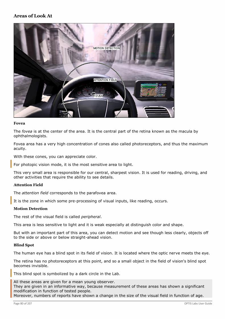
Page 80 of 207 OPTIS Labs User Guide
Areas of Look At
Fovea
The fovea is at the center of the area. It is the central part of the retina known as the macula by
ophthalmologists.
Fovea area has a very high concentration of cones also called photoreceptors, and thus the maximum
acuity.
With these cones, you can appreciate color.
For photopic vision mode, it is the most sensitive area to light.
This very small area is responsible for our central, sharpest vision. It is used for reading, driving, and
other activities that require the ability to see details.
Attention Field
The attention field corresponds to the parafovea area.
It is the zone in which some pre-processing of visual inputs, like reading, occurs.
Motion Detection
The rest of the visual field is called peripheral.
This area is less sensitive to light and it is weak especially at distinguish color and shape.
But with an important part of this area, you can detect motion and see though less clearly, objects off
to the side or above or below straight-ahead vision.
Blind Spot
The human eye has a blind spot in its field of vision. It is located where the optic nerve meets the eye.
The retina has no photoreceptors at this point, and so a small object in the field of vision's blind spot
becomes invisible.
This blind spot is symbolized by a dark circle in the Lab.
All these areas are given for a mean young observer.
They are given in an informative way, because measurement of these areas has shown a significant
modification in function of tested people.
Moreover, numbers of reports have shown a change in the size of the visual field in function of age.

Labs Page 81 of 207
Vision Parameters
Using Vision Parameters
With Vision Parameters, you can change the map point fixed by the observer or the physical
characteristics of the eye.
1. Click Tools, Vision parameters ....
-Or-
1. Click .
A window appears.
2. Set the parameters see page 81.
3. Click OK.
You can select the Automatic update check box to compute data in real time.
4. Click Close.
Parameters of Vision Parameters
Modelisation Parameters
In Modelisation parameters group box, you can select physical phenomena that can be taken into
account in the luminance map display.
By selecting the Depth of field check box, you can simulate the depth of field.
This model takes into account physical properties of the eye, like focal length and pupil diameter,
and accommodation distance.
Accommodation distance corresponds to the distance between the observer and the object that the
observer is looking at.
Following images are a scene made up of two tests of vision separated by a distance from two
meters. The observer is placed at one meter of the nearest test.

Page 82 of 207 OPTIS Labs User Guide
Accommodation distance = 10 m Accommodation distance = 5 m
Accommodation distance = 3 m Accommodation distance = 1 m
The pupil size is given in an automatic way, starting from the average luminance of the luminance
map. This can be modified.
For post-processing, the diameter of the pupil is three millimeters.
By selecting the Visual acuity check box, you can model the acuity according to the level of
luminance.
Visual acuity diminishes when the luminance decreases.
Visual acuity is computed according to the level of light for each fovea area.
For more details about fovea, you can view Areas of Look At see page 80.
Dark area are displayed with a worst resolution than bright area to reflect the loss of acuity of the
fovea area when luminance decreases.
With visual acuity Without visual acuity
Visual acuity depends directly on the average level of luminance of the simulated scene. Indeed,
cones density and distribution on the retina are not similar to rods one.
Thus, there is a significant modification of visual acuity when one passes from the photopic
conditions of observation in the mesopic conditions.

Labs Page 83 of 207
Average luminance of the map = 20 cd/m² Average luminance of the map = 0.05
cd/m²
In order that this filtering has perceptible effects, it is necessary to have a luminance map with
significant angular resolutions (relationship between the number of pixel and the angle of view).
By selecting the Peripheral acuity check box, the loss of the eye space resolution according to
the image's position on the retina is taking into account.
In this case, fovea acuity is only computed for the vision center.
The distribution of the cones on the retina decreases from the center of the retina towards the
periphery.
It results in a variation of the visual acuity according to the position on the retina.
The following images show results obtained when one takes into account the distribution and the
density of the cones on the retina.
The luminance maps used are the same than in the Depth of field example.
For left and middle images, the central point of vision is the center of the luminance map. This can
be modified and it is possible to indicate any points of the map as being the new fixation point.
On the right image, the fixation point corresponds to the letter T.
In following images, you can see the fixation point displacement.
Note that the luminosity of the images is high to better visualize the effects of acuity loss.
The maximum map luminance is of approximately 1.e-3 cd/m².

Page 84 of 207 OPTIS Labs User Guide
By selecting the Glare effect check box, you can activate the glare effect.
For more details about the glare effect, you can view Glare Effect Overview see page 86.
You must select Vos, 1984 or Holladay, 1926.
Vos,1984 is partly based on Vos, J. Disability glare - a state of the art report. C.I.E. Journal 3, 2
(1984), 39-53.
Vos,1984 takes into account the light scattering into the cornea, the lens and the retina of the eye
responsible for the veil of luminance.
It also simulates the lenticular halo and the ciliary corona essentially caused by the lens.
Holladay,1926 is partly based on the work described in Holladay,Journal of the Optical Society of
America, 12, 271 (1926) and P. Moon, D. Spencer, The Visual Effect of Non-Uniform Surrounds,
Journal of the Optical Society of America, vol. 35, No. 3, pp. 233-248 (1945).
Holladay,1926 takes only into account scattering into the cornea, the lens and the retina.
Without glare effect Vos,1984 Holladay,1926
Eye Adaptation
In Adaptation type box, you can select Local adaptation or Dynamic adaptation.
With Local adaptation, the accommodation is on a fixed point of the luminance map.
You can change the luminance value of this point in Cd/m². When you open a luminance map, this
value is equal to the average luminance of the map.
You can click Default to restore this value.
With Dynamic adaptation, you can model spatial adaptation of the human eye.
This model is equivalent to the fact that the eye adapts locally as the viewer scan the different regions
of the luminance map.
Dynamic adaptation method can be significantly more expensive than local adaptation techniques.
When selecting Dynamic adaptation, you can modify the condition of observation of the scene.
You can click Default to restore initial values.

Labs Page 85 of 207
Condition of Observation of the Scene
In Condition of observation of the scene group box, you can take into account the fact that it takes
some times for the observer to adapt to the average luminance of the current luminance map when the
observer is adapted to a luminance L0.
In Previous adaptation luminance box, you can change the luminance L0 value in Cd/m² at which
the observer is adapted before seeing the current luminance map.
In Observation time box, you can change the time value in seconds during which the observer sees
the current luminance map.
In Age of the observer box, you can change the age of the observer in years which is taking into
account to evaluate contrast sensitivity, glare and time adaptation.
You can click Default to restore initial values.
The default Previous adaptation luminance value is the mean luminance of the map and the default
Observation time value is a very long time equal to three thousands seconds.
Here the observer is fully adapted to the current luminance map.
Vision Mode Evaluation is Based on
In Vision mode evaluation is based on group box, you can define how the vision mode photopic,
mesopic, or scotopic is estimated.
Vision mode defines the photoreceptors sensitivity. As an example for photopic vision, rods are fully
saturated.
By selecting Average value of the xmp, vision mode is computed using the mean luminance value of
the map.
The rods saturation state is supposed to be the same for all the point of the luminance map.
By selecting Maximum value of the xmp, vision mode is computed using the maximum luminance
value of the map.
The rods saturation state is supposed to be the same for all the point of the luminance map.
By selecting Each point of the xmp, vision mode is computed using the mean luminance value of the
map and the result displayed in the status bar.
But in each point of the luminance map, rod saturation state is computed using the luminance value of
the pixel.
Eye Parameters
In the Eye parameters group box, you can click to clear the Automatic evaluation check box.
In the Aperture box, you can type the pupil diameter value in millimeters.
In the Focal length box, you can type the value of the equivalent focal distance from the eye in
millimeters.
By selecting the Automatic evaluation check box, it automatically calculates eye parameters.
The pupil diameter is estimated from the displayed map luminance and a focal distance is defined from
an average eye.
Vision Center
In Vision center group box, you can define the point of the map fixed by the observer.
In Point at box, the value refers to the fixed point compared to the center of the luminance map.
In Accommodation distance box, you can enter accommodation distance value in millimeters.
You can click to select a pixel in the map. It updates the accommodation distance value.
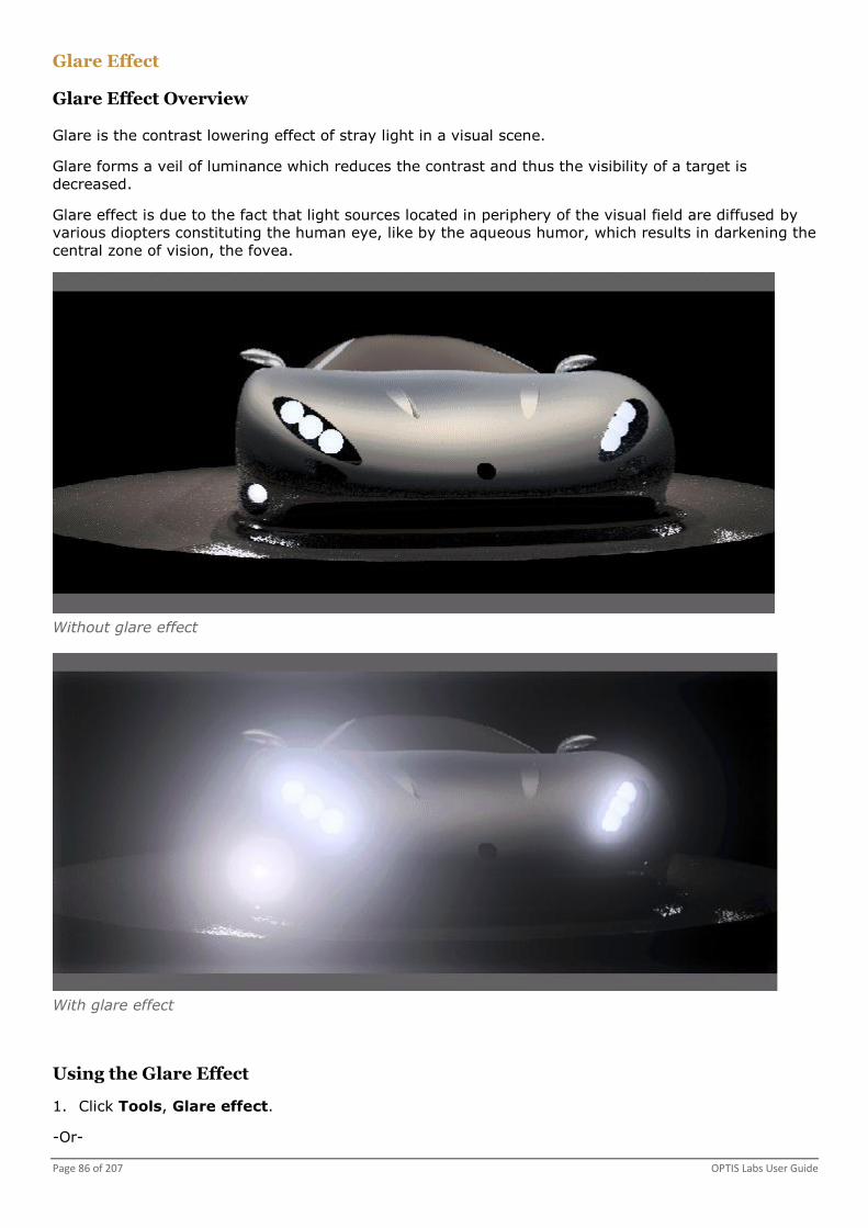
Page 86 of 207 OPTIS Labs User Guide
Glare Effect
Glare Effect Overview
Glare is the contrast lowering effect of stray light in a visual scene.
Glare forms a veil of luminance which reduces the contrast and thus the visibility of a target is
decreased.
Glare effect is due to the fact that light sources located in periphery of the visual field are diffused by
various diopters constituting the human eye, like by the aqueous humor, which results in darkening the
central zone of vision, the fovea.
Without glare effect
With glare effect
Using the Glare Effect
1. Click Tools, Glare effect.
-Or-

Labs Page 87 of 207
1. Click .
-Or-
1. From the Vision parameters window, select the Glare Effect check box .
For more details about Vision parameters window, you can view Using Vision Parameters see
page 81.
Doing Time Adaptation
With Time adaptation, you can generate an AVI file which includes successive images seen by a human
adapted to a specified luminance level L0 and seeing the current luminance map.
If the difference between the luminance L0 and the mean luminance of the map is very high, it takes
some time for the observer to adapt to the new luminance.
The AVI file shows the image variation perceived by the observer during this time.
Previous Adaptation Luminance
In Previous adaptation luminance box, you must type the luminance value of the time adaptation
area with L0 luminance in Cd/m².
Filename
In Filename box, you must browse the path and type the name of the AVI file.
If needed, you can select the Flip vertically check box.
Adaptation
You must click Adaptation to generate the AVI file.
If the observer is adapted at a very high luminance and observes a luminance map with a very low
mean luminance, the time adaptation is called dark adaptation and the adaptation can take until
thirty minutes. That’s why the time of the AVI file is compressed , the real time is displayed in the
left top of the AVI.
If the observer is adapted to a very low luminance and observe a luminance map with a very high
luminance the time adaptation is called light adaptation and takes few seconds.
The first image of the AVI file shows the previous luminance adaptation state and the mean
luminance value of the current luminance map.
The AVI stops when the observer is totally adapted to the luminance map.
Time adaptation only uses the dynamic adaptation mode.
Doing Analysis
The human eye has a high range of luminance detection. It is able to detect luminance level from 10-6
cd/m² to 108 cd/m².
Displays do not have such a high dynamic.

Page 88 of 207 OPTIS Labs User Guide
The Virtual Human Vision Lab includes specific functions able to display the final image as if the scene
is seen by a human. The luminance map compression is required.
With Analysis tools, you can have information on the luminance distribution of the map, and on the
level of compression.
Click Tools, Analysis... to display the Analysis tools window.
Analysis tools depends on the eye adaptation.
For more details about eye adaptation, you can view Parameters of Vision Parameters see page 81.
The fovea luminance histogram shows the distribution of luminance for the current XMP file.
For more details about fovea, you can view Areas of Look At see page 80.
The fovea luminance is computed into a solid angle of about 1°, so the luminance map is
subdivided into solid angle of 1°.
The histogram shows for each luminance value, the number of fovea area of the map having this
luminance.
The Display luminance according to scene luminance diagram shows the relationship between the
map luminance and the display luminance.
If it is a dynamic adaptation, the diagram depends on the fovea luminance histogram.
Here the compression of the luminance map is made to take into account human vision properties,
and to allocate the maximum of display dynamic for luminance area with a high number of areas.
For luminance value for which histogram contains a lot of values, the curve slope of the diagram is
very high.
Dynamic adaptation
If it is a local adaptation, the diagram only depends on the adaptation luminance.

Labs Page 89 of 207
For more details about adaptation luminance, you can view Parameters of Vision Parameters see
page 81.
Local adaptation
Legibility and Visibility Analysis
Using Legibility and Visibility Tools
1. Click Tools, Legibility/Visibility tools ....
A window appears.
2. Set the parameters see page 89.
3. Close the window.
Parameters of Legibility and Visibility Tools
Legibility and Visibility Tools give additional information regarding results.
Legibility (CIE 145:2002 standard)
Legibility (CIE 145:2002 standard) tab gives the relative visual performance of an observer according
to different parameters.
With Legibility (CIE 145:2002 standard) tab, you can indicate if a letter selected in a luminance map
can be read.

Page 90 of 207 OPTIS Labs User Guide
Legibility (CIE 145:2002 standard) tab applies the CIE 145: 2002 The correlation of models for vision
and visual performance standard.
Letter Luminance
In Letter luminance box, you can type the luminance value of the letter in cd/m².
If needed, you can click to select a pixel in the map.
If needed, you can click to clear the previous selection.
Background Luminance
In Background luminance box, you can type the luminance value of the background in Cd/m².
If needed, you can click to select a pixel in the map.
If needed, you can click to clear the previous selection.
If needed, you can click to display colorimetric coordinates when using .
Current color is related to the letter coordinates described by a black cross on the diagram.
Reference color is related to the background coordinates described by a red cross on the diagram.
DeltaE indicates colorimetric gap between letter and background. DeltaE value should be higher than
100 to get good legibility.
Colorimetric gap between target and background is low message appears when the DeltaE value
is inferior to one hundred value using the DeltaE Luv formula.
This value is defined to have a good readability of the letter using the MILSTD1472F norm, 5.2.1.5.6.4
paragraph.
For more details about colorimetric data, you can view Parameters of Chromaticity Coordinates Tool
see page 44.
If needed, you can select the Automatic update check box to update luminance each time the
luminance map is modified.
Size of the Critical Detail
In Size of the critical detail box, you can set the size of the letter by typing the angle subtended by
the critical detail of the letter in minutes of arc.
As an example, critical detail of the letter can be the stroke widths.
The CIE regulation recommends measuring the letter height or stroke width.
Size is calculated using the observer position and the map size.
If needed, you can click to evaluate the size of the critical detail.
A line is displayed in the luminance map to adjust the extreme points.
Observer Age
In Observer age box, you can type the age of the observer in years.
Contrast
In Contrast box, you can read the contrast value calculated from the formula recommended by the
CIE 145:2002 regulation.
Contrast = (Luminance of the background- Luminance of the letter)/ Luminance of the background
Relative Visual Performance
In Relative visual performance box, you can read the relative visual performance value.
Relative visual performance is also called RVP.

Labs Page 91 of 207
Relative visual performance is measured using the size of the critical detail and the observer age.
The value is between 0 and 1.
RVP = 1 is normalized to the performance level of an adult of twenty years old reading critical detail
sizes of 4.5 minutes of arc with an average luminance of 1000 cd/m².
The relative visual performance is defined as a proportional measure of visual performance potential
expressed in terms of the maximum value achievable.
Curve Options
In Curve options group box, you can select the option to display the Relative visual performance
diagram according to the observer age, the background luminance, the letter luminance, the letter size
or the contrast.
When selecting Contrast, you can select Background luminance is constant or Letter luminance
is constant.
Surface Tool
In Surface tool box, you can click to select a letter using a displayed rectangle in the luminance
map.
You must click or to select if your text is in positive or negative contrast.
If needed, you can click Update to computed letter luminance, background luminance and letter size.
You can select the Automatic update check box to computed data in real time.
Visibility
With Visibility tab, you can evaluate the visibility of an object having an angular size superior to 4
degrees.
The object can be as an example a reflection into a windshield.
This evaluation is partly based on the work done by Blackwell. References are Blackwell, H.R. Contrast
threshold of the human eye, Journal of the optical society of America 1946, 36, 624-643.
Previous Adaptation Luminance
In Previous adaptation luminance box, you can type the luminance (L0) value at which the
observer is adapted before seeing the current object. Value is in cd/m².
Observation Time
In Observation time box, you can type the time during which the observer has been adapted to the
luminance L0. Value is in seconds.
Observer Age
In Observer age box, you can type the age of the observer in years.
Background Luminance
In Background luminance box, you can type the luminance value of the background around the
target in cd/m².
If needed, you can click to select a pixel in the map.
If needed, you can click to clear the previous selection.
Target Luminance
In Target luminance box, you can type the luminance value of the object for which you want to
analyze visibility in cd/m².

Page 92 of 207 OPTIS Labs User Guide
If needed, you can click to select a pixel in the map.
If needed, you can click to clear the previous selection.
Curve Options
In Curve options group box, you can select the option to display the visibility diagram with delta
luminance in cd/m² in function of the background luminance in cd/m².
Delta luminance is equal to the difference between background luminance and target luminance.
Visibility state box gives information if the target is visible.
Using Sun Glasses / Colored Filter
You must have a spectral xmp map to use Sun glasses or Colored filter.
With Sun glasses or Colored filter, you can select sun glasses spectrum or colored filter.
The transmission values contained in the file are in percent.
1. Click Tools, Sun glasses or Colored filter ....
A box appears.
2. Select the Activate check box.
3. Click to browse a .spectrum or .spe file.
If needed, you can click to display the spectrum.
4. Click Apply.
5. Close the box.

Labs Page 93 of 207
Sunglasses spectrum
Without glasses

Page 94 of 207 OPTIS Labs User Guide
With sunglasses - Category 3
Night Vision Goggles
Using Night Vision Goggles
You must have a spectral xmp map to use Night vision goggles.
1. Click Tools, Night vision goggles ....
A box appears.
2. Select the Activate check box.
3. Set the parameters see page 94.
You can open or save a file containing night vision goggles data. In this case you can save your
data as a .nvg file.
4. Click Apply.
Calculation time can be quite long because of the spectral data's treatment.
Parameters of Night Vision Goggles
Technology
In Technology box, you can select night vision goggles of generation II (Gen II) or generation III
(Gen III).
With Gen III class A, B or C, you can define a NVG of generation III with a filter in the objective lens to
restrict the response in the visible range.
Class A defines a 625nm minus blue filter.
Class B defines a 665nm minus blue filter.
Class C defines a leaky green filter.
Field of View
In Field of view, you must set the field of view value in degrees.
The field of view is the spatial angle of the outside scene that can be viewed through night vision
goggles.
System Resolution
In System Resolution box, you must set the resolution value in cycles per milliradians.
The system resolution at the center of the image is the ability of night vision goggles to distinguish
between objects close together.
Image intensifier resolution is measured in line pairs per millimeter (lp/mm) while system resolution is
measured in cycles per milliradian (cy/mr).
For any particular night vision system, the image intensifier resolution remains constant while the
system resolution can be affected by altering the objective or eyepiece optics by adding magnification
or relay lenses.
Signal to Noise Ratio
In Signal to noise ratio box, you must type a ratio value.
Signal to Noise Ratio is also called SNR.
A measure of the light signal reaching the eye divided by the perceived noise as seen by the eye.

Labs Page 95 of 207
A tube's SNR determines the low light resolution of the image tube. Therefore higher is the SNR, better
is the ability of the tube to resolve objects with good contrast under low light conditions.
System Luminance Gain
In System luminance gain box, you must type the luminance gain value.
System luminance gain is the ratio of NVG output's luminance to input's luminance. Units are in foot-
lamberts.
A typical value for a GEN III tube is 5,000 fL/fL.
Max. Average Output Luminance
In Max. average output luminance box, you must type the maximal average output luminance
value in foot-lamberts.
Maximal average output luminance is the maximal output luminance averaged across the full field of
view.
When observed luminance increases, the luminance system gain is reduced to keep average luminance
of the phosphor screen below this value.
Phosphor Screen Spectrum
In Phosphor screen spectrum box, you must click to browse a .spectrum or .spe file to define
the spectrum of the phosphor screen.
If needed, you can click to display the spectrum.
Additional Filter
In Additional filter box, you must click to browse a .spectrum or .spe file to simulate a filter
used in the input of the night vision goggle.
If needed, you can click to display the spectrum.
Surface and Section Analysis
Making Surface and Section Analysis
With Surface and Section Analysis tool, you can have several information as total flux, contrast,
average luminance or brightness inside a surface which can be a rectangle, a polygon or an ellipse. You
can also display image section.
1. Click Tools, Surface...
-Or-
1. Click .
A box appears and a shape appears on your map.
2. Set the parameters see page 95.
Close the window.
Parameters of Surface and Section Analysis
Units are automatically set depending on the type of map: luminance (cd/m²) or relative brightness.
Shape
You must select a type of shape as Rectangle, Ellipse or Polygon to define the analysis surface.

Page 96 of 207 OPTIS Labs User Guide
You can select the Surface 3D check box to enable the 3D view display of the image.
When right-clicking, the 3D Chart Control Properties box appears.
You can click ChartGroup to configure display options.
You can click Axes to configure axes and add grid lines by clicking GridLines.
You can click Levels to change levels and colors.
You can click Control, Save... to save values.
In case of a spectral map, you can view spectrum data , colorimetric data or color rendering
index .
Center
In Center group box, you must type values to define the position of the analysis surface.
Note that you can use the mouse to set center values.
Dimensions
In Dimensions group box, you must type values to define the dimension of the analysis surface.
Note that you can use the mouse to set dimensions values.
Section
You can enable the analysis section. A line is drawn on the map and a box opens to display the curve.
From the map display, you can move horizontal, vertical or user lines.
Data over a line can be exported to a .txt file by clicking Export....
Maximum / Minimum
You can read maximum and minimum values of the analysis surface.
Average
You can read average value for the shape or section belong to the following formula.
V is the value in one pixel.
W is the weight of V, ratio between the pixel surface in the calculation area and the total surface of the
pixel.
N is the number of measurement points.
Barycenter X / Barycenter Y
You can read barycenter X and barycenter Y values belong to the following formula.
x and y are the pixel coordinates.
Eye Illuminance
You can read the eye illuminance value.
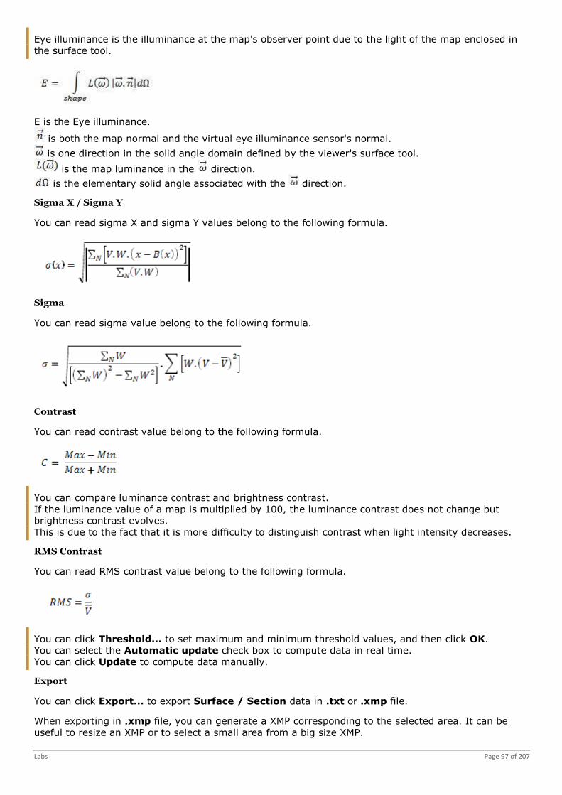
Labs Page 97 of 207
Eye illuminance is the illuminance at the map's observer point due to the light of the map enclosed in
the surface tool.
E is the Eye illuminance.
is both the map normal and the virtual eye illuminance sensor's normal.
is one direction in the solid angle domain defined by the viewer's surface tool.
is the map luminance in the direction.
is the elementary solid angle associated with the direction.
Sigma X / Sigma Y
You can read sigma X and sigma Y values belong to the following formula.
Sigma
You can read sigma value belong to the following formula.
Contrast
You can read contrast value belong to the following formula.
You can compare luminance contrast and brightness contrast.
If the luminance value of a map is multiplied by 100, the luminance contrast does not change but
brightness contrast evolves.
This is due to the fact that it is more difficulty to distinguish contrast when light intensity decreases.
RMS Contrast
You can read RMS contrast value belong to the following formula.
You can click Threshold... to set maximum and minimum threshold values, and then click OK.
You can select the Automatic update check box to compute data in real time.
You can click Update to compute data manually.
Export
You can click Export... to export Surface / Section data in .txt or .xmp file.
When exporting in .xmp file, you can generate a XMP corresponding to the selected area. It can be
useful to resize an XMP or to select a small area from a big size XMP.
Page 98 of 207 OPTIS Labs User Guide
You can then export as a .txt file.
For an extended map (data separated by source or surface) or a spectral map (data separated by
wavelength), the exported file includes one line for each source (or surface) or wavelength.
The format of the exported file is:
The same header as when you export the XMP map in a TXT file,
A line for the surface or the line definition:
Surface=Rectangle Left=value Top=value Right=value Bottom=value
-Or-
Surface=Ellipse CenterX=value CenterY=value RayX=value RayY=value
-Or-
Surface=Polygon PtNumber=n Pt0_X=value Pt0_Y=value... Ptn_X=value Ptn_Y=value
-Or-
Line Pt0_X=value Pt0_Y=value Pt1_X=value Pt1_Y=value Sampling=value
A column header:
(Source) (Wavelength) XMax YMax Max XMin YMin Min Average Contrast Sigma Flux BarycentreX
BarycentreY SigmaX SigmaY
-Or-
(Source) (Wavelength) XMax YMax Max XMin YMin Min Average Contrast Sigma
The data:
Basic map: One line
Extended map:
line 1 => User
line 2 => All
line 3 => Data for source 0
line 4 => Data for source 1
...
Spectral map:
line 1 => All
line 2 => Data for wavelength 0
line 3 => Data for wavelength 1
line 4 => Data for wavelength 2
...
Virtual Lighting Controller
Using the Virtual Lighting Controller
To use Virtual Lighting Controller, you must have a map with data separated by source, by surface or
sequence (extended or spectral).
With Virtual Lighting Controller, you can change contribution of layers without running new simulation.
Layers can be sources, surfaces or sequence.
1. Click Tools, Virtual Lighting Controller ...
-Or-
1. Click .
A box appears.
2. Set the parameters see page 99.
3. Close the box.

Labs Page 99 of 207
Parameters of the Virtual Lighting Controller
If needed, you can change layers' name.
You can select the Automatic update check box to compute data in real time.
You can click Update to compute data manually.
You can click Select all or Unselect all to respectively select or unselect all the layers.
If needed, you can add or delete a new sliders configuration.
When it is enabled, you can select Power to display power instead of ratio.
In case of spectral map, you can change units using the View menu.
For spectral maps, you can click to display a layer's spectrum.
The option is not available for ambient sources, LCD sources and set of sources including sources
which do not have the same spectrum.
The spectrum change has to be used carefully in case of fluorescent surface.
Vertical lines correspond to the spectral sampling of the xmp.
Click to define a new light source spectrum.
The spectrum of the new source is normalized to get the same power than the initial source. Unit is
photometric or radiometric depending on the one defined in the View menu.
Initial xmp Result after the spectrum change
With , you can delete a spectrum.
This function is only available in the Virtual Photometric Lab, Virtual Human Vision Lab and 3D
Energy Density Lab.
With , you get information a new spectrum has been added.
With , you can get back previous spectrum.
With , you get information a spectral data has not been saved in xmp map.
The spectral sampling of the xmp should be sufficient to cover spectrum of the new layer.
Spectrum of the initial layer should not be null within all spectral zone on each the new spectrum is
not null.
Spectrum changes can take a lot of time because calculations have been made directly on spectral
data of xmp map. When you change a spectrum for the first time, all spectral data are downloaded
in the memory and all modified calculations of layers powers are made on the spectral data. This
can take more time than usual. To avoid this when you do not need any new spectrum change but
only power change, you can clear the View, Load spectral data option.

Page 100 of 207 OPTIS Labs User Guide
Editing the Preferences
1. Click Tools, Preferences....
-Or-
1. Click .
A window appears.
2. Set the preferences see page 194.
Virtual Photometric Lab
With Virtual Photometric Lab, you can visualize spectral luminance maps and display an image for each
wavelength.
Using the Virtual Photometric Lab
Virtual Photometric Lab is compatible with OLE Automation standard so that you can use a language
like VBScript to get information stored into XMP maps.
For more details, you can view Virtual Photometric Lab.
1. From Start menu, click All Programs, OPTIS, OPTIS Labs, Labs, Virtual Photometric Lab.
-Or-
1. Click Virtual Photometric Lab .
A window appears.
You can open or save a XMP map file. In this case you can save your XMP map as a .xmp file.
You can print the XMP map file.
You can import see page 101 or export see page 103 a file.
You can also import a BMP mask see page 101.
You can display results, manage display options see page 110.
Click to read map properties. For more details about precision, you can view Reading Precision
see page 111.
You can analyze colorimetric data see page 76.
You can make surface and section analysis see page 112.
Click Tools, Pick value.... to get value at a specific position.
Click or Tools, Zernike to display Zernike coefficients.
You can use the Virtual Lighting Controller see page 115.
For spectral xmp maps, you can use sun glasses or colored filter see page 117 and you can use
Night Vision Goggles see page 94.
You can edit preferences see page 119.
You can manage the filtering see page 119.
All following operations are multi threaded: Open, Standard filtering, Remove highest peaks
filtering, Map addition and multiplication by a value (Photometric Calc and Distributed Computing),
Surface/Section calculations and Display update.
The threads number used for these operations is the number of processors (including cores) of the
computer.
Labs Page 101 of 207
Importing and Exporting
Importing
Importing an Image
1. Click File, Import....
A window appears.
2. Browse an image.
The image can have one of the following formats.
FILES EXTENSIONS
Bitmap .bmp
Text .txt
Technoteam luminance image .pf
Technoteam color image .cos
OpenEXR .exr
RGBE .hdr, .pic
For more details about .txt files, you can view TXT File Format see page 104.
For more details about .hdr files, you can view HDRI File Format see page 71.
Files data have to be in the XYZ format.
If the Operation not supported message appears, the colorimetric space in the technoteam
software has to be set on XYZ.
If the imported map is uniform, the regional preferences of windows have to be set to have point
instead of comma.
3. Click Open .
4. If the image is a .bmp, .hdr or.pic file, a window appears. Set the parameters see page 101 and
click OK.
5. If the image is a .pf file, a window appears. Set the parameters see page 103 and click OK.
Importing a BMP Mask
1. Click File, BMP mask import....
A box appears.
2. Browse a .bmp file.
3. Click Open .
A window appears.
4. Set the parameters see page 101.
5. Click OK.
Parameters of Bitmap or RGBE Import
When importing bitmap file and converting it as map, the map can be used as emittance for source
definition.
The emittance of a source describes how each point of a surface emits rays.
For a source definition, the emittance can be uniform or described by a basic or a spectral map.
In the case of a basic map you have to supply a spectrum for the source and this spectrum is the same

Page 102 of 207 OPTIS Labs User Guide
for each point of the source.
In the case of a spectral map, the spectrum for the source is generated from the color of each pixel of
the bitmap.
Importing bitmap file is very useful to define an environment around your system for a real rendering
(luminance simulation).
There is an infinite possible spectrum for one color and the bitmap file import only provides a solution
with three Gaussian spectrum centered on red, green and blue. In most cases, default options gives a
good resulting XMP map.
Bitmap File
In Bitmap file box, you can change the bitmap file.
Map Type
In Map type group box, you must select the map type.
With Basic map, you can convert the selected bitmap into a basic xmp map.
With Laser map, you can convert the selected bitmap into a basic laser xmp map. You can then select
Amplitude check box. If needed you can select Phase check box and browse a .bmp file. In
Wavelength box, you must set the wavelength value in nanometers.
With Spectral map, you can convert the selected bitmap into a spectral xmp map. In Wavelength
minimum, Wavelength maximum, Wavelength Nb and Wavelength Step boxes, you must set
values to define the wavelength's sampling for converting a color bitmap into a spectral map. In Red
spectrum, Green spectrum and Blue spectrum boxes, you must browse to select spectrum files for
converting a color bitmap into a spectral map.
Dimensions
In Dimensions group box, you must set the width and height of the converted xmp map in
millimeters.
You can select the Respect ratio check box to keep ratio between width and height.

Labs Page 103 of 207
Parameters of Technoteam PF File Import
Technoteam luminance images are generated from Technoteam photometric camera.
These files contain a luminance image.
Dimensions
In Dimensions group box, you must set the width and height of the image in millimeters.
This information could be found using Technoteam software delivered with the photometric camera.
You can select the Respect ratio check box to keep ratio between width and height.
Exporting
Exporting an Image
You must open an image first.
1. Click File, Export....
A window appears.
2. Type a file name and select a format.
The image can have one of the following formats.
FILES EXTENSIONS
Xmp map .xmp
Bitmap .bmp
JPeg .jpg
PNG .png
Tiff .tiff
Text .txt
Technoteam luminance image .pf
Excel .xls

Page 104 of 207 OPTIS Labs User Guide
FILES EXTENSIONS
OpenEXR .exr
RGBE .hdr
For more details about .txt files, you can view TXT File Format see page 104.
For more details about .hdr files, you can view HDRI File Format see page 71.
OpenEXR and RGBE are only enable in case of spectral maps.
3. Click Save .
4. In case of a .xmp file export, a box appears. Set the parameters see page 74 and click OK.
5. In case of a .txt file export, a box appears. Select Export data by layer or Merge active
layer(s). Click OK.
For more details, you can view Extended Map Format see page 105.
Parameters of XMP Export
The xmp Export is like a Save As except that the export includes options.
These options help to reduce the file's size on the disk.
If you do not need to analyze the spectrum on each pixel of the map and if you do not need to
analyze the data for each wavelength, you can select Include spectral data check box.
If you want to group some sources data of the map, you can select Merge active layer(s) check
box.
If you want to have filtered or original data in the exported file, you can select Export filtered
data check box.
If you want to export a spectral map to convert it into an extended map, you can select
Conversion to extended map check box.
You can select Intensity normalized as luminance check box and set a value for the Surface
box in square millimeters.
TXT File Format
With TXT file import, you can precisely define the emittance of any sources. As an example, TXT file
can be generated with a camera.
The format of the ASCII file is the same for import and export.
MapType
ValueType Intensitytype
UnitType
AxisUnit
XMin XMax YMin YMax
NbX NbY
WMin WMax NbW (Spectral map)
SourceNb Ratio0 Ratio1... RatioNb (Extended map)
x0y0 x1y0 x2y0 ... xny0
x0y1 x1y1 x2y1 ... xny1
x0y2 x1y2 x2y2 ... xny2
...
x0yn x1yn x2yn ... xnyn
Option preceding by // are not supported at that time.
MapType can have one of the following values.
OptisMapTypeBasic = 0
//OptisMapTypeLaser = 1

Labs Page 105 of 207
OptisMapTypeSpectral = 2
OptisMapTypeExtended = 3
//OptisMapTypeUnknown = 4
//OptisMapTypeGainMatrix = 5
ValueType can have one of the following values.
OptisValueTypeIrradiance = 0
OptisValueTypeIntensity = 1
OptisValueTypeRadiance = 2
//OptisValueTypeSel = 3
//OptisValueTypeLaserPhase = 4
//OptisValueTypeLaserPhasePlane = 5
//OptisValueTypeDirectionalIrradiance = 6
//OptisValueTypeGain = 7
Intensitytype can have one of the following values.
OptisIntensityOptis = 0
OptisIntensitySAETypeA = 1
OptisIntensitySAETypeB = 2
OptisIntensityConoscopic = 3
If ValueType is not equal to 1, the IntensityType value is not taken into account.
For Intensity Conoscopic format, you must be aware that transformation takes into account following
formulas.
TetaX = Teta.cos Phi
TetaY = Teta.sin Phi
UnitType can have one of the following values.
OptisUnitTypeRadiometric = 0
OptisUnitTypePhotometric = 1
//OptisUnitTypeGain = 2
//OptisUnitTypeUnknown = 3
AxisUnit can have one of the following values.
//OptisUnitDefault = 0
OptisUnitMillimeter = 1
OptisUnitDegree = 2
OptisUnitRadian = 3
OptisUnitFeet = 4
//OptisUnitMicrons = 5
//OptisUnitNanometer = 6
//OptisUnitMeter = 7
For intensity maps, XMin XMax YMin YMax has to be replaced by ThetaXMin ThetaXMax
ThetaYMin ThetaYMax.
Extended Map Format
When exporting TXT file format, it is possible to merge enable sources.
MapType (3 for an extended map)
ValueType
UnitType
AxisUnit
XMin XMax YMin YMax (For an intensity map: ThetaXMin ThetaXMax ThetaYMin ThetaYMax)
NbX NbY
In case of extended map with no merged sources, the format is as following.
LayerNb LayerInitialPower0 LayerInitialPower1... LayerInitialPowerNb
Source_Name_1
x0y0s1 x1y0s1 x2y0s1 ... xny0s1
x0y1s1 x1y1s1 x2y1s1 ... xny1s1
x0y2s1 x1y2s1 x2y2s1 ... xny2s1

Page 106 of 207 OPTIS Labs User Guide
Source_Name_2
x0y0s2 x1y0s2 x2y0s2 ... xny0s2
x0y1s2 x1y1s2 x2y1s2 ... xny1s2
x0y2s2 x1y2s2 x2y2s2 ... xny2s2
In case of extended map with merged sources, the format is as following.
-1 LayerNb LayerInitialPower0 LayerInitialPower1... LayerInitialPowerNb
SourceRatio1 SourceRatio2 ... SourceRatioN
x0y0 x1y0 x2y0 ... xny0
x0y1 x1y1 x2y1 ... xny1
x0y2 x1y2 x2y2 ... xny2
With -1 value before LayerN, you can know if the extended map has been included in an enable
sources's merge.
If sources are not merged, you do not have to enter any values. In this case, sources power and their
ratio are not taking into account. You must not use it for the import because it means there is only one
enable source and you can not use a basic map. This parameter is useful as information when
exporting an extended map with a merge of enable sources.
In case of spectral map with merged sources, the format is as following.
WMin WMax NbW
SeparatedByLayer SourceRatio1 SourceRatio2 ... SourceRatioN
Layer_Name
x0y0w0 x1y0w0 x2y0w0 ... xny0w0
x0y1w0 x1y1w0 x2y1w0 ... xny1w0
x0y2w0 x1y2w0 x2y2w0 ... xny2w0
x0y0w1 x1y0w1 x2y0w1 ... xny0w1
x0y1w1 x1y1w1 x2y1w1 ... xny1w1
x0y2w1 x1y2w1 x2y2w1 ... xny2w1
...
x0y0wN x1y0wN x2y0wN ... xny0wN
x0y1wN x1y1wN x2y1wN ... xny1wN
x0y2wN x1y2wN x2y2wN ... xny2wN
In case of spectral map with no merged sources, the format is as following.
WMin WMax NbW
SeparatedByLayer LayerNb RadiometricPowerofSource1 PhotometricPowerofSource1 ...
RadiometricPowerofSourceN PhotometricPowerofSourceN
Layer_Name_1
x0y0w0 x1y0w0 x2y0w0 ... xny0w0
x0y1w0 x1y1w0 x2y1w0 ... xny1w0
x0y2w0 x1y2w0 x2y2w0 ... xny2w0
x0y0w1 x1y0w1 x2y0w1 ... xny0w1
x0y1w1 x1y1w1 x2y1w1 ... xny1w1
x0y2w1 x1y2w1 x2y2w1 ... xny2w1
...
x0y0wN x1y0wN x2y0wN ... xny0wN
x0y1wN x1y1wN x2y1wN ... xny1wN
x0y2wN x1y2wN x2y2wN ... xny2wN
Layer_Name_2
x0y0w0 x1y0w0 x2y0w0 ... xny0w0
x0y1w0 x1y1w0 x2y1w0 ... xny1w0
x0y2w0 x1y2w0 x2y2w0 ... xny2w0
x0y0w1 x1y0w1 x2y0w1 ... xny0w1
x0y1w1 x1y1w1 x2y1w1 ... xny1w1
x0y2w1 x1y2w1 x2y2w1 ... xny2w1
...
x0y0wN x1y0wN x2y0wN ... xny0wN
x0y1wN x1y1wN x2y1wN ... xny1wN
x0y2wN x1y2wN x2y2wN ... xny2wN
...
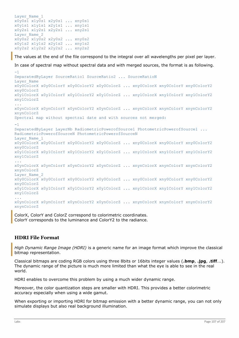
Labs Page 107 of 207
Layer_Name_1
x0y0s1 x1y0s1 x2y0s1 ... xny0s1
x0y1s1 x1y1s1 x2y1s1 ... xny1s1
x0y2s1 x1y2s1 x2y2s1 ... xny2s1
Layer_Name_2
x0y0s2 x1y0s2 x2y0s2 ... xny0s2
x0y1s2 x1y1s2 x2y1s2 ... xny1s2
x0y2s2 x1y2s2 x2y2s2 ... xny2s2
The values at the end of the file correspond to the integral over all wavelengths per pixel per layer.
In case of spectral map without spectral data and with merged sources, the format is as following.
-1
SeparatedByLayer SourceRatio1 SourceRatio2 ... SourceRatioN
Layer_Name
x0y0ColorX x0y0ColorY x0y0ColorY2 x0y0ColorZ ... xny0ColorX xny0ColorY xny0ColorY2
xny0ColorZ
x0y1ColorX x0y1ColorY x0y1ColorY2 x0y1ColorZ ... xny1ColorX xny1ColorY xny1ColorY2
xny1ColorZ
...
x0ynColorX x0ynColorY x0ynColorY2 x0ynColorZ ... xnynColorX xnynColorY xnynColorY2
xnynColorZ
Spectral map without spectral date and with sources not merged:
-1
SeparatedByLayer LayerNb RadiometricPowerofSource1 PhotometricPowerofSource1 ...
RadiometricPowerofSourceN PhotometricPowerofSourceN
Layer_Name_1
x0y0ColorX x0y0ColorY x0y0ColorY2 x0y0ColorZ ... xny0ColorX xny0ColorY xny0ColorY2
xny0ColorZ
x0y1ColorX x0y1ColorY x0y1ColorY2 x0y1ColorZ ... xny1ColorX xny1ColorY xny1ColorY2
xny1ColorZ
...
x0ynColorX x0ynColorY x0ynColorY2 x0ynColorZ ... xnynColorX xnynColorY xnynColorY2
xnynColorZ
Layer_Name_2
x0y0ColorX x0y0ColorY x0y0ColorY2 x0y0ColorZ ... xny0ColorX xny0ColorY xny0ColorY2
xny0ColorZ
x0y1ColorX x0y1ColorY x0y1ColorY2 x0y1ColorZ ... xny1ColorX xny1ColorY xny1ColorY2
xny1ColorZ
...
x0ynColorX x0ynColorY x0ynColorY2 x0ynColorZ ... xnynColorX xnynColorY xnynColorY2
xnynColorZ
ColorX, ColorY and ColorZ correspond to colorimetric coordinates.
ColorY corresponds to the luminance and ColorY2 to the radiance.
HDRI File Format
High Dynamic Range Image (HDRI) is a generic name for an image format which improve the classical
bitmap representation.
Classical bitmaps are coding RGB colors using three 8bits or 16bits integer values (.bmp, .jpg, .tiff...).
The dynamic range of the picture is much more limited than what the eye is able to see in the real
world.
HDRI enables to overcome this problem by using a much wider dynamic range.
Moreover, the color quantization steps are smaller with HDRI. This provides a better colorimetric
accuracy especially when using a wide gamut.
When exporting or importing HDRI for bitmap emission with a better dynamic range, you can not only
simulate displays but also real background illumination.

Page 108 of 207 OPTIS Labs User Guide
Today, HDRI are supported by most rendering programs to export the rendering results but also to
import environment map. Environment maps enable to achieve very realistic illuminations. OPTIS
software are able to use environment maps (cube or sphere HDRI maps) to achieve comparable result
and even better result thanks to its physics based calculation.
You can generate good environment HDRI maps using digital cameras and a software tool like
HDRShop.
Supported Formats
RGBE and OpenEXR are supported formats.
RGBE is the native Radiance format. This is the most wide used format today.
ILM 's OpenEXR is the most powerful format to date.
XMPs are even better than HDRI, including spectral data, source separation...
When exporting XMP to HDRI your are able to address the full dynamic provided by HDRI which is not
possible when exporting a BMP to HDRI with a classical rendering software.
XMP export to HDRI: 16 bits to 16 bits
BMP export to HDRI: 8 bits to 16 bits
HDRI/Classical Bitmap Comparison
Here is a picture having levels divided by two at each step from the left to the right.
Only the left most columns are visible, the other are too dark to be seen. To see the rest of the picture,
one has to saturate the visible part by changing the exposure.
Let us compare what happen if the picture is HDRI (on the right) and if the picture is a classical bitmap
(on the left).
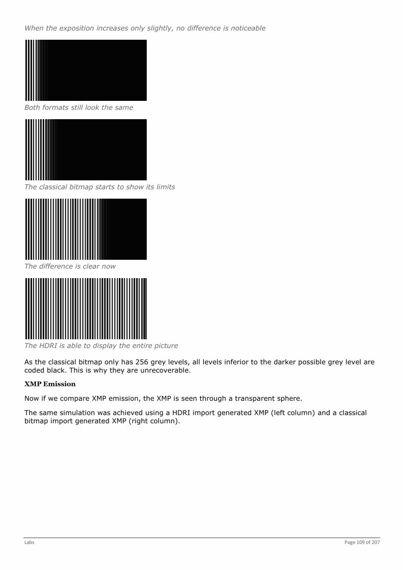
Labs Page 109 of 207
When the exposition increases only slightly, no difference is noticeable
Both formats still look the same
The classical bitmap starts to show its limits
The difference is clear now
The HDRI is able to display the entire picture
As the classical bitmap only has 256 grey levels, all levels inferior to the darker possible grey level are
coded black. This is why they are unrecoverable.
XMP Emission
Now if we compare XMP emission, the XMP is seen through a transparent sphere.
The same simulation was achieved using a HDRI import generated XMP (left column) and a classical
bitmap import generated XMP (right column).

Page 110 of 207 OPTIS Labs User Guide
The Virtual Photometric Lab level indicates the light level that is displayed saturated.
Virtual Photometric Lab level = 2 500 cd/m²
Virtual Photometric Lab level = 10 000 cd/m²
Managing the Display
All display's options as filtering level, Surface/Section parameters or layers' configurations are saved
within the Virtual Photometric map when saving the file.
If you want to move the map, left-click and move the mouse at the same time.
If you want to make a vertical or horizontal symmetry of the map, click Operation, Vertical axis
symmetry or Horizontal axis symmetry.
If you want to use the zoom, rotate the mouse wheel, click Edit, Activate Zoom or click and
then left-click or right-click.
Click to display the original size.
When moving the mouse over the map, values at the position are displayed in the status bar.
The displayed value is interpolated with the value of many pixels. Click View, Interpolate values to
activate or deactivate the interpolation.
If you want to view spectrum curve at the mouse position, click .

Labs Page 111 of 207
If you want to modify the number format, right-click on the status bar.
The number format is the number of decimal per value.
If you want to modify the unit belong to the map type, click View, Photometric units or
Radiometric units.
If you want to modify the axis unit of displayed values, right-click on the status bar.
If you want to change displayed colors, use the color list.
Iso levels displays the image with ISO curves or surfaces.
If you want to display Wavefront Error or FFT MTF or PSF, use the Wavefront Error list.
If you to change displayed field, use the field list.
If you want to display one single wavelength, use the wavelength list.
If you want to display grids and other options, right-click on the map to select tools.
As an example you can show ruler, set ruler parameters, show axis on cross, snap cross to grid,
show tooltip, show gray around the map, fill shape, show primary or secondary graduations, set
graduations parameters, show primary or secondary grids, set grid parameters.
If you want to modify display's parameters, click Tools, Level... or .
You can select a level to modify the value. Press Enter to validate the change.
You can right-click and select Copy to clipboard.
When modifying minimum or maximum value, you can select the Intermediate levels auto-
update check box to compute all intermediate values.
If needed, you can add or delete a color level.
You can click Default to cancel all modifications.
Select the IsoCurve and Filled check boxes, to display the image with or without ISO curves.
Click Linear or Log to switch between a linear or logarithmic scale.
Click Load Scale or Save Scale to load or save parameters in an OPTIS scale file. Format is .scl.
When Iso levels is selected in the color list, you can change the color between two levels clicking
.
Reading Precision
Precision Value
In direct simulation, the displayed precision value corresponds to the pixel having the highest number
of integrated rays.
Precision formula is the following.
Precision = 1/sqrt(N)
With N the number of rays integrated by the pixel.
When no rays are integrated on a pixel, the error is infinite. The precision value is one hundred
percent.
In direct simulation using radiance luminance sensor with activated gathering, precision does not have
any meaning. Precision value is also one hundred percent.
In inverse simulation using the Monte-Carlo algorithm, a number of pass has to be specified as 100
passes = 100 rays per pixel (not necessary effective rays).
Precision formula is the following.
Precision = 1/sqrt(N)
With N the number of passes.
In inverse simulation using determinist or photon map algorithms, precision does not have any
meaning. Precision value is also one hundred percent.
Page 112 of 207 OPTIS Labs User Guide
Higher is the precision percent, lower is the image quality.
Be aware that one pixel which has not received any rays or which has received only one has a one
hundred percent precision.
More rays or passes there are, lower is the statistical noise. A direct correlation between this number
and the error (or variance, standard deviation) is not possible.
For systems under weighted Monte-Carlo algorithms, the only way to compute error (variance) is to
launch the same simulation several times and to calculate the standard deviation of specific pixels.
The statistical error is always less important for pixels with more integrated rays.
Precision Map
For direct simulation, you can click Tools, Precision map... to display the precision map.
The precision map is only validate for all sources set at one hundred percent when there is no any
separation by sources.
The precision is displayed in percent and is saved in rays number in the map. You can then generate
precision calculation with the surface / section analysis tool.
Analyzing Colorimetric Data
Three tools are available to analyze colorimetric data.
If you want to see colorimetric data at a specific pixel location, you can click Tools, Colorimetric
data... or .
For more details, you can view Parameters of Chromaticity Coordinates Tool see page 44.
If you want to analyze the error between the color displayed by the screen and the reality for all
points of the map, you can click Tools, Colorimetric error....
The true color luminance map is replaced by a colorimetric error map displayed in false color.
When the dynamic of the luminance map is higher than the one of the screen, the Lab compresses
the luminance using a linear relation.
With colorimetric error tool, you can analyze the error between the color after compression and the
color really displayed by the screen.
The colorimetric error is calculated using the CIE94 (1 :1 :1) formula (CIE 116-1995).
When the dynamic of the luminance map is lower than the one of the display, there is no
luminance compression. In this case the displayed error is the one between the color contained in
the luminance map and the one really displayed.
If you want to have all information about the spectrum for all points of the map, you can click
Tools, Spectrum... or .
For more details, you can view Spectrum Editor see page 49.
If you want to read the color rendering index values, you can click Tools, Color Rendering Index
(CRI) ....
For more details, you can view Parameters of the Color Rendering Index see page 51.
Surface and Section Analysis
Making Surface and Section Analysis
With Surface and Section Analysis tool, you can have several information as total flux, contrast,
average inside a surface which can be a rectangle, a polygon or an ellipse. You can also display image
section.

Labs Page 113 of 207
1. Click Tools, Surface...
-Or-
1. Click .
A box appears and a shape appears on your map.
2. Set the parameters see page 113.
3. Close the window.
Parameters of Surface and Section Analysis
Units are automatically set depending on the type of map (luminance, illuminance...).
Shape
You must select a type of shape as Rectangle, Ellipse or Polygon to define the analysis surface.
You can select the Surface 3D check box to enable the 3D view display of the image.
When right-clicking, the 3D Chart Control Properties box appears.
You can click ChartGroup to configure display options.
You can click Axes to configure axes and add grid lines by clicking GridLines.
You can click Levels to change levels and colors.
You can click Control, Save... to save values.
In case of a spectral map, you can view spectrum data , colorimetric data or color rendering
index .
Center
In Center group box, you must type values to define the position of the analysis surface.
Note that you can use the mouse to set center values.
Dimensions
In Dimensions group box, you must type values to define the dimension of the analysis surface.
Note that you can use the mouse to set dimensions values.
Section
You can enable the analysis section. A line is drawn on the map and a box opens to display the curve.
From the map display, you can move horizontal, vertical or user lines.
Data over a line can be exported to a .txt file by clicking Export....
Maximum / Minimum
You can read maximum and minimum values of the analysis surface.
Average
You can read average value for the shape or section belong to the following formula.
V is the value in one pixel.
W is the weight of V, ratio between the pixel surface in the calculation area and the total surface of the

Page 114 of 207 OPTIS Labs User Guide
pixel.
N is the number of measurement points.
Flux
You can read flux value in the shape belong to the following formula.
S is the surface of the calculation area.
Sp is the surface of one pixel.
Barycenter X / Barycenter Y
Barycenter X and Y values are not useful for conoscopic maps.
You can read barycenter X and barycenter Y values belong to the following formula.
x and y are the pixel coordinates.
Sigma X / Sigma Y
You can read sigma X and sigma Y values belong to the following formula.
Sigma
You can read sigma value belong to the following formula.
Contrast
You can read contrast value belong to the following formula.
RMS Contrast
You can read RMS contrast value belong to the following formula.
You can click Threshold... to set maximum and minimum threshold values, and then click OK.
You can select the Automatic update check box to compute data in real time.
You can click Update to compute data manually.

Labs Page 115 of 207
Export
You can click Export... to export Surface / Section data in .txt or .xmp file.
When exporting in .xmp file, you can generate a XMP corresponding to the selected area. It can be
useful to resize an XMP or to select a small area from a big size XMP.
You can then export as a .txt file.
For an extended map (data separated by source or surface) or a spectral map (data separated by
wavelength), the exported file includes one line for each source (or surface) or wavelength.
The format of the exported file is:
The same header as when you export the XMP map in a TXT file,
A line for the surface or the line definition:
Surface=Rectangle Left=value Top=value Right=value Bottom=value
-Or-
Surface=Ellipse CenterX=value CenterY=value RayX=value RayY=value
-Or-
Surface=Polygon PtNumber=n Pt0_X=value Pt0_Y=value... Ptn_X=value Ptn_Y=value
-Or-
Line Pt0_X=value Pt0_Y=value Pt1_X=value Pt1_Y=value Sampling=value
A column header:
(Source) (Wavelength) XMax YMax Max XMin YMin Min Average Contrast Sigma Flux BarycentreX
BarycentreY SigmaX SigmaY
-Or-
(Source) (Wavelength) XMax YMax Max XMin YMin Min Average Contrast Sigma
The data:
Basic map: One line
Extended map:
line 1 => User
line 2 => All
line 3 => Data for source 0
line 4 => Data for source 1
...
Spectral map:
line 1 => All
line 2 => Data for wavelength 0
line 3 => Data for wavelength 1
line 4 => Data for wavelength 2
...
Virtual Lighting Controller
Using the Virtual Lighting Controller
To use Virtual Lighting Controller, you must have a map with data separated by source, by surface or
sequence (extended or spectral).
With Virtual Lighting Controller, you can change contribution of layers without running new simulation.
Layers can be sources, surfaces or sequence.

Page 116 of 207 OPTIS Labs User Guide
1. Click Tools, Virtual Lighting Controller ...
-Or-
1. Click .
A box appears.
2. Set the parameters see page 116.
3. Close the box.
Parameters of the Virtual Lighting Controller
If needed, you can change layers' name.
You can select the Automatic update check box to compute data in real time.
You can click Update to compute data manually.
You can click Select all or Unselect all to respectively select or unselect all the layers.
If needed, you can add or delete a new sliders configuration.
When it is enabled, you can select Power to display power instead of ratio.
In case of spectral map, you can change units using the View menu.
For spectral maps, you can click to display a layer's spectrum.
The option is not available for ambient sources, LCD sources and set of sources including sources
which do not have the same spectrum.
The spectrum change has to be used carefully in case of fluorescent surface.
Vertical lines correspond to the spectral sampling of the xmp.
Click to define a new light source spectrum.
The spectrum of the new source is normalized to get the same power than the initial source. Unit is
photometric or radiometric depending on the one defined in the View menu.
Initial xmp Result after the spectrum change
With , you can delete a spectrum.
This function is only available in the Virtual Photometric Lab, Virtual Human Vision Lab and 3D
Energy Density Lab.
With , you get information a new spectrum has been added.
Labs Page 117 of 207
With , you can get back previous spectrum.
With , you get information a spectral data has not been saved in xmp map.
The spectral sampling of the xmp should be sufficient to cover spectrum of the new layer.
Spectrum of the initial layer should not be null within all spectral zone on each the new spectrum is
not null.
Spectrum changes can take a lot of time because calculations have been made directly on spectral
data of xmp map. When you change a spectrum for the first time, all spectral data are downloaded
in the memory and all modified calculations of layers powers are made on the spectral data. This
can take more time than usual. To avoid this when you do not need any new spectrum change but
only power change, you can clear the View, Load spectral data option.
Using Sun Glasses or Colored Filter
You must have a spectral xmp map to use Sun glasses or Colored filter.
With Sun glasses or Colored filter, you can select sun glasses spectrum or colored filter.
The transmission values contained in the file are in percent.
1. Click Tools, Sun glasses or Colored filter ....
A box appears.
2. Select the Activate check box.
3. Click to browse a .spectrum or .spe file.
If needed, you can click to display the spectrum.
4. Click Apply.
5. Close the box.
Night Vision Goggles
Using Night Vision Goggles
You must have a spectral xmp map to use Night vision goggles.
1. Click Tools, Night vision goggles ....
A box appears.
2. Select the Activate check box.
3. Set the parameters see page 94.
You can open or save a file containing night vision goggles data. In this case you can save your
data as a .nvg file.
4. Click Apply.
Calculation time can be quite long because of the spectral data's treatment.
Parameters of Night Vision Goggles
Technology
In Technology box, you can select night vision goggles of generation II (Gen II) or generation III
(Gen III).

Page 118 of 207 OPTIS Labs User Guide
With Gen III class A, B or C, you can define a NVG of generation III with a filter in the objective lens to
restrict the response in the visible range.
Class A defines a 625nm minus blue filter.
Class B defines a 665nm minus blue filter.
Class C defines a leaky green filter.
Field of View
In Field of view, you must set the field of view value in degrees.
The field of view is the spatial angle of the outside scene that can be viewed through night vision
goggles.
System Resolution
In System Resolution box, you must set the resolution value in cycles per milliradians.
The system resolution at the center of the image is the ability of night vision goggles to distinguish
between objects close together.
Image intensifier resolution is measured in line pairs per millimeter (lp/mm) while system resolution is
measured in cycles per milliradian (cy/mr).
For any particular night vision system, the image intensifier resolution remains constant while the
system resolution can be affected by altering the objective or eyepiece optics by adding magnification
or relay lenses.
Signal to Noise Ratio
In Signal to noise ratio box, you must type a ratio value.
Signal to Noise Ratio is also called SNR.
A measure of the light signal reaching the eye divided by the perceived noise as seen by the eye.
A tube's SNR determines the low light resolution of the image tube. Therefore higher is the SNR, better
is the ability of the tube to resolve objects with good contrast under low light conditions.
System Luminance Gain
In System luminance gain box, you must type the luminance gain value.
System luminance gain is the ratio of NVG output's luminance to input's luminance. Units are in foot-
lamberts.
A typical value for a GEN III tube is 5,000 fL/fL.
Max. Average Output Luminance
In Max. average output luminance box, you must type the maximal average output luminance
value in foot-lamberts.
Maximal average output luminance is the maximal output luminance averaged across the full field of
view.
When observed luminance increases, the luminance system gain is reduced to keep average luminance
of the phosphor screen below this value.
Phosphor Screen Spectrum
In Phosphor screen spectrum box, you must click to browse a .spectrum or .spe file to define
the spectrum of the phosphor screen.
If needed, you can click to display the spectrum.

Labs Page 119 of 207
Additional Filter
In Additional filter box, you must click to browse a .spectrum or .spe file to simulate a filter
used in the input of the night vision goggle.
If needed, you can click to display the spectrum.
Editing the Preferences
1. Click Tools, Preferences... .
A window appears.
2. Set the preferences see page 194.
Managing the Filtering
With Filtering, you can smooth the map and use several analysis tools.
Using the XMP Filtering
By clicking Filtering, XMP Filtering, you can modify the map data by applying a filtering on the data.
The filtering algorithm modifies the value of each pixel with the values of its neighbors.
Depending on the map type, different types of XMP filtering are available.
When selecting Standard, you can do XMP filtering for basic or extended maps. It only uses
neighbors without any considerations regarding values of these neighbors.
When selecting Remove highest peaks, you can do XMP filtering for spectral maps. It removes very
high values which could appear in a very noisy map.
In Threshold box, you must type the threshold value.
If the pixel value is threshold times higher or lower than the average value of its neighbors, a
median filtering is applied to the pixel.
When selecting Anisotropic, it uses neighbors taking into account the values of these neighbors and
it diffuses modifications.
Anisotropic filtering is used to filter low dynamic images. Using high dynamic images can generate
problems and change colors.
Anisotropic filtering is a filter algorithm that keeps objects edge in the image to avoid blur. It
computes the mean of neighboring pixels according an edge detection criteria.
It acts as if the pixels influence spreads on its neighbors circularly in uniform regions, and
elliptically in edge regions in order to keep borders.
Filter shape when arriving near an image's border
At each diffusion pass, a diffusion step is applied in two directions.
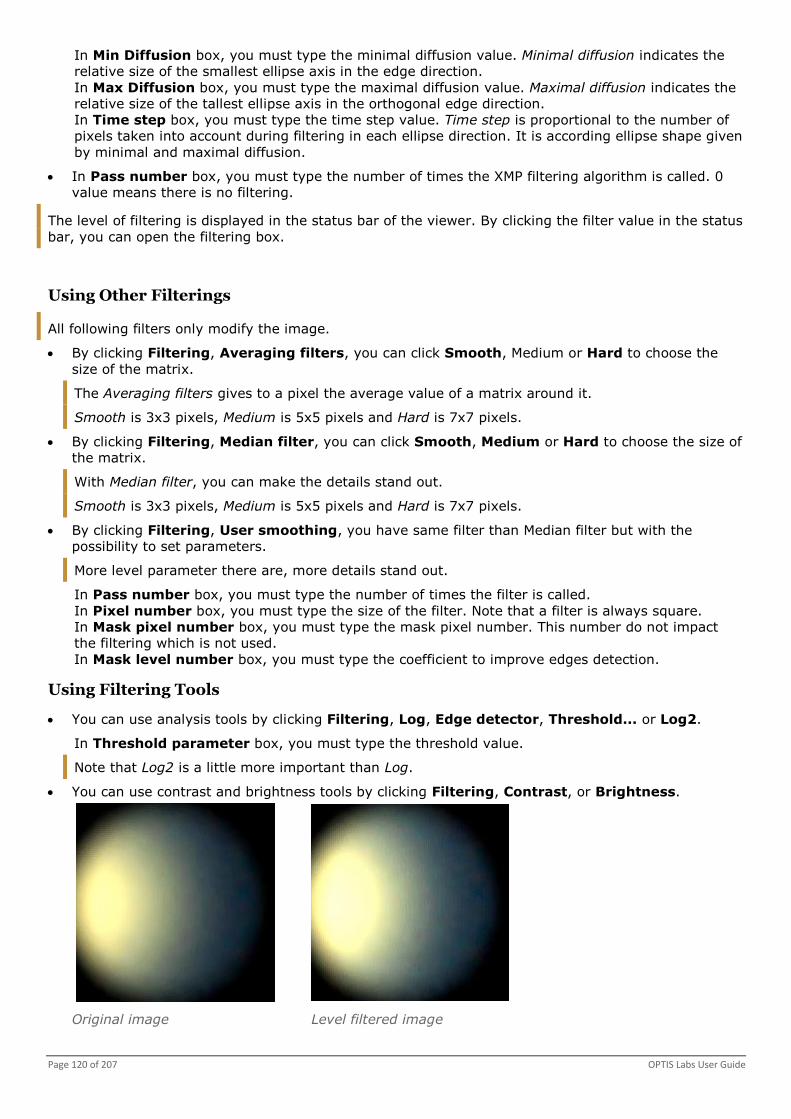
Page 120 of 207 OPTIS Labs User Guide
In Min Diffusion box, you must type the minimal diffusion value. Minimal diffusion indicates the
relative size of the smallest ellipse axis in the edge direction.
In Max Diffusion box, you must type the maximal diffusion value. Maximal diffusion indicates the
relative size of the tallest ellipse axis in the orthogonal edge direction.
In Time step box, you must type the time step value. Time step is proportional to the number of
pixels taken into account during filtering in each ellipse direction. It is according ellipse shape given
by minimal and maximal diffusion.
In Pass number box, you must type the number of times the XMP filtering algorithm is called. 0
value means there is no filtering.
The level of filtering is displayed in the status bar of the viewer. By clicking the filter value in the status
bar, you can open the filtering box.
Using Other Filterings
All following filters only modify the image.
By clicking Filtering, Averaging filters, you can click Smooth, Medium or Hard to choose the
size of the matrix.
The Averaging filters gives to a pixel the average value of a matrix around it.
Smooth is 3x3 pixels, Medium is 5x5 pixels and Hard is 7x7 pixels.
By clicking Filtering, Median filter, you can click Smooth, Medium or Hard to choose the size of
the matrix.
With Median filter, you can make the details stand out.
Smooth is 3x3 pixels, Medium is 5x5 pixels and Hard is 7x7 pixels.
By clicking Filtering, User smoothing, you have same filter than Median filter but with the
possibility to set parameters.
More level parameter there are, more details stand out.
In Pass number box, you must type the number of times the filter is called.
In Pixel number box, you must type the size of the filter. Note that a filter is always square.
In Mask pixel number box, you must type the mask pixel number. This number do not impact
the filtering which is not used.
In Mask level number box, you must type the coefficient to improve edges detection.
Using Filtering Tools
You can use analysis tools by clicking Filtering, Log, Edge detector, Threshold... or Log2.
In Threshold parameter box, you must type the threshold value.
Note that Log2 is a little more important than Log.
You can use contrast and brightness tools by clicking Filtering, Contrast, or Brightness.
Original image Level filtered image

Labs Page 121 of 207
Contrast filtered image Brightness filtered image
For more details about the level tool, you can view Managing the Display see page 110.
Virtual Reality Lab
With Virtual Reality Lab, you can read natively OpenEXR/HDR and XMP spectral picture and OPTIS
environment map (OptisVR).
You can visualize a HDR environment map and create it with six pictures of your simulation (HDR or
XMP spectral).
Moreover, you can use the virtual lighting controller to change source level of lights on picture and
environment map.
Finally, with Virtual Reality Lab, you can export the result to HDR/EXR/OptisVR and QTVR formats.
Virtual Reality Lab Icons
You can open a file (EXR, HDR, XMP (only spectral format) and OptisVR).
You can save the current file.
You can use the Virtual Lighting Controller.
For more details, you can view Using Virtual Lighting Controller see page 123.
With Maximal Level Controller, you can change the maximal level of the
picture or environment map.
Colorimetric Data.
Human Vision.
Vision Parameters.
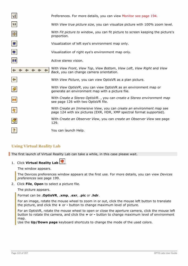
Page 122 of 207 OPTIS Labs User Guide
Preferences. For more details, you can view Monitor see page 194.
With View true picture size, you can visualize picture with 100% zoom level.
With Fit picture to window, you can fit picture to screen keeping the picture's
proportion.
Visualization of left eye's environment map only.
Visualization of right eye's environment map only.
Active stereo vision.
With View Front, View Top, View Bottom, View Left, View Right and View
Back, you can change camera orientation.
With View Picture, you can view OptisVR as a plan picture.
With View OptisVR, you can view OptisVR as an environment map or
generate an environment map with a picture file.
With Create a Stereo OptisVR. , you can create a Stereo environment map
see page 126 with two OptisVR file.
With Create an Immersive View, you can create an environment map see
page 124 with six pictures (EXR, HDR, XMP spectral format supported).
With Create an Observer View, you can create an Observer View see page
129.
You can launch Help.
Using Virtual Reality Lab
The first launch of Virtual Reality Lab can take a while, in this case please wait.
1. Click Virtual Reality Lab .
The window appears.
The Devices preferences window appears at the first use. For more details, you can view Devices
preferences see page 199.
2. Click File, Open to select a picture file.
The picture appears.
Format can be .OptisVR, .xmp, .exr, .pic or .hdr.
For an image, rotate the mouse wheel to zoom in or out, click the mouse left button to translate
the picture, and click the + or - button to change maximum level of picture.
For an OptisVR, rotate the mouse wheel to open or close the aperture camera, click the mouse left
button to rotate the camera, and click the + or - button to change maximum level of environment
map.
Use the Up/Down page keyboard shortcuts to change the mode of the used colors.

Labs Page 123 of 207
Virtual Lighting Controller
Using the Virtual Lighting Controller
To use Virtual Lighting Controller, you must have a map with data separated by source, by surface or
sequence (extended or spectral).
With Virtual Lighting Controller, you can change contribution of layers without running new simulation.
Layers can be sources, surfaces or sequence.
1. Click Edit, Virtual Lighting Controller ...
-Or-
1. Click .
A box appears.
2. Set the parameters see page 123.
3. Close the box.
Parameters of the Virtual Lighting Controller VRL
If needed, you can change layers' name.
You can select the Automatic update check box to compute data in real time.
You can click Update to compute data manually.
You can click Select all or Unselect all to respectively select or unselect all the layers.
If needed, you can add or delete a new sliders configuration.
When it is enabled, you can select Power to display power instead of ratio.
In case of spectral map, you can change units using the View menu.
For spectral maps, you can click to display a layer's spectrum.
The option is not available for ambient sources, LCD sources and set of sources including sources
which do not have the same spectrum.
The spectrum change has to be used carefully in case of fluorescent surface.
Vertical lines correspond to the spectral sampling of the xmp.
Click to define a new light source spectrum.
The spectrum of the new source is normalized to get the same power than the initial source. Unit is
photometric or radiometric depending on the one defined in the View menu.

Page 124 of 207 OPTIS Labs User Guide
Initial xmp Result after the spectrum change
With , you can delete a spectrum.
This function is only available in the Virtual Photometric Lab, Virtual Human Vision Lab and 3D
Energy Density Lab.
With , you get information a new spectrum has been added.
With , you can get back previous spectrum.
With , you get information a spectral data has not been saved in xmp map.
The spectral sampling of the xmp should be sufficient to cover spectrum of the new layer.
Spectrum of the initial layer should not be null within all spectral zone on each the new spectrum is
not null.
Spectrum changes can take a lot of time because calculations have been made directly on spectral
data of xmp map. When you change a spectrum for the first time, all spectral data are downloaded
in the memory and all modified calculations of layers powers are made on the spectral data. This
can take more time than usual. To avoid this when you do not need any new spectrum change but
only power change, you can clear the View, Load spectral data option.
Creating an Immersive View
Immersive View is when the eyes are looking around them.
Immersive view is an environment map with six pictures.
Immersive view's format is Optis VR.
1. Click Create an Immersive View .
-Or-
1. Click the Creation menu, Create an Immersive View.
A window appears.
2. Select the wanted picture, and then double-left-click.
3. Browse a picture file.
The first loaded picture configures the environment map (size of picture, format and number of
sources).
Only one picture has to be uploaded.
The environment map with six pictures appears.
If you want to rotate a picture, you can use the rotation menu.
You can change the Maximal Level.
4. Click OK.
5. Save the Immersive View.
The Immersive View appears.
Human Vision
Using Human Vision
1. Click Edit, Human Vision...
-Or-
2. Click .

Labs Page 125 of 207
The Human vision is now enabled.
3. Click Edit, Human Vision Parameters...
-Or-
4. Click .
A box appears.
5. Set the parameters see page 125.
Parameters of Human Vision
You can select an Adaptation type from the list.
Select Local adaptation so that the accommodation is on a fixed point of the luminance map.
Use the slider in the Local Adaptation Properties box to change the luminance value of this
point in Cd/m² . When you open a luminance map, this value is equal to the average luminance
of the map.
You can click Default to reset adaptation luminance.
Select Dynamic adaptation to enable the spatial adaptation of the human eye.
This models the fact that the eye adapts locally as the viewer scans the different areas of the
luminance map.
You can select the Automatic update check box to compute automatically the ideal adapted
luminance for the scene.
This option is automatically activated for Dynamic Adaptation. It disables the Local Adaptation
Properties box for the Local Adaptation type.
You can select the Temporal adaptation check box to enable human eye time adaptation which
occurs on scene luminance changes.
This option is available only for Dynamic Adaptation.
Example of Temporal adaptation (in mm:ss)
You can select a Mesopic calculation mode from the list to define how the photopic, mesopic or
scotopic vision mode is estimated.
This defines the photoreceptors sensitivity.
As an example for photopic vision rods are fully saturated.
You can select Maximum. With this parameter the vision mode is computed using the
maximum luminance value of the scene. Rods saturation state is supposed to be the same for
all points of the luminance map.

Page 126 of 207 OPTIS Labs User Guide
You can select Average. With this parameter vision mode is computed using the mean value of
the scene. Rods saturation state is supposed to be the same for all points of the luminance map.
You can select the Glare Effect (Vos 1984) check box to activate the glare effect.
Vos 1984 is partly based on Vos, J. Disability glare – a state of the art report. C.I.E Journal 3,
2(1984), 39-53.
Vos 1984 takes into account the light scattering into the cornea, the lens and the retina of the eye
responsible for the veil of luminance.
It also simulates the lenticular halo and the ciliary corona essentially caused by the lens.
Without glare effect Vos, 1984
You can edit the Age of the observer group box to change the observer’s age in years.
This option is available only when Dynamic Temporal Adaption or Glare Effect are enabled.
Stereo OptisVR
Creating a Stereo OptisVR
Stereo OptisVR is saved in .OptisVR format.
1. Click Create a Stereo OptisVR .
-Or-
2. Click Creation, Create a Stereo OptisVR.
A window appears.
3. Browse a left .OptisVR file.
4. Browse a right .OptisVR file.
Files must have same dimensions and sources' number.
5. Click OK.
6. Save the Stereo OptisVR.
The Stereo OptisVR appears.
You can use the + and - buttons to optimize the rendering.
You can click View left eye or View right eye to switch between left and right eye's
environment map.
You can click View in 3D Stereo to activate the stereo mode.
This option is only enabled when using a graphics card supporting the active stereo (for example
QUADRO model for NVIDIA).
Active Stereoscopy (Frame sequential mode)
One projector displays right and left images in frame sequential mode.

Labs Page 127 of 207
The end-user wears shutter glasses that occult each eye after the other according to the display
framerate.
Passive Stereoscopy
Passive view can be used in one or several screens. When using one screen, a graphic card with two
output LCD projectors is needed (not available for LCD screen).
When using several screens, two projectors equipped with special filters displaying right and left
images are needed. End-user wears passive stereo glasses and look at screens.
1. Open the Multiscreen tool.
2. Set one Display, one Window, two Areas and two Eyes for the Avatar.
3. Save.
4. Click Run.

Page 128 of 207 OPTIS Labs User Guide
5. Select a stereo OptisVR file.
Using the Stereo Immersive View Correction
This tool can only be used with an Immersive View see page 124.
By default, the focal plane is at the infinite.
With Stereo Immersive View Correction, you can set the stereo focus distance to optimize the
visualization.
1. Click File, Open or click Open to launch a Stereo OptisVR file.
2. In case of the active stereoscopy, click View in 3D Stereo to activate the stereo mode.
3. In case of the passive stereoscopy, use the Multiscreen to activate the stereo mode.
4. Click View, Set Focal plane.
A window appears.
5. Move the slider to align an area.
This sets the focal plane at this location.
Focal Plane on the acronym Focal Plane on the rear-view mirror

Labs Page 129 of 207
Switching between Stereo and Normal Mode
It is possible to switch between Stereo and Normal Mode in Full Screen mode.
To do it, you can use the following shortcuts:
r Right eye
l Left eye
s Stereo mode
Creating an Observer View
Observer View is when eyes are turning around the object.
In the simulation several cameras should have been placed around the object and should look at the
same point.
Result of the simulation has to be a list of images using the XMP format.
Images should have same dimensions and same number of sources.
1. Click Create an Observer View .
-Or-
2. Click Creation, Create an Observer View.
3. Click Open and then select a list of .xmp files.
The number of selected images can be limited by the computer memory.
4. Click OK.
5. Save the view as an .OptisVR file.
The Observer View appears.
You can use the + and - buttons to optimize the rendering.
You can turn the view with the mouse.
Virtual Reality Lab Management
Switching Between HDRI Picture and Immersive View
Converting HDRI Picture to Immersive View
If you load a picture with 4:3, 3:4, 1:6 proportion, you can transform this picture to Immersive View.
1. Click View Immersive .
The picture changes.
This option is only enabled if the conversion is possible.
A picture with 4:3, 3:4, 1:6 proportion is not necessarily a valid cubemap.
Converting Immersive View to HDRI Picture
1. Click View Picture .
The picture changes.

Page 130 of 207 OPTIS Labs User Guide
Using the Filtering
The Filtering option is used to reduce noise of the picture.
1. Click Edit, Filtering.
Saving Results
Save As
OPENING FORMAT SAVING FORMAT
PICTURE
EXR
HDR
XMP (spectral)
EXR
HDR
OptisVR
OPTISVR/OPTISVR
OptisVR Environment map
mode
OptisVR
Picture mode EXR HDR
OptisVR Stereo OptisVR Stereo
Export to QTVR
Save OptisVR to Quicktime VR format (.mov).
This function is only enabled with Virtual Reality Lab 32bits.
MultiScreen
The Master Mode manages the simulation and the Slave Mode executes the orders.
The slave is always used on a separated computer.
A directory including .OptisVR files has to be shared between Master and Slave. Used path has to go
through the Network.
Slaves must have the required rights to connect to this shared directory. This means that the slave
does no have to connect to the directory with a login and password.
System VR Configuration
System VR Configuration Overview
System VR Configuration is composed of Windows, Areas and SystemDisplay itself composed of
Displays and Avatars.
Real World Virtual World
Cave SystemDisplay
Cave's wall Display
Human/Machine
in the Cave Avatar

Labs Page 131 of 207
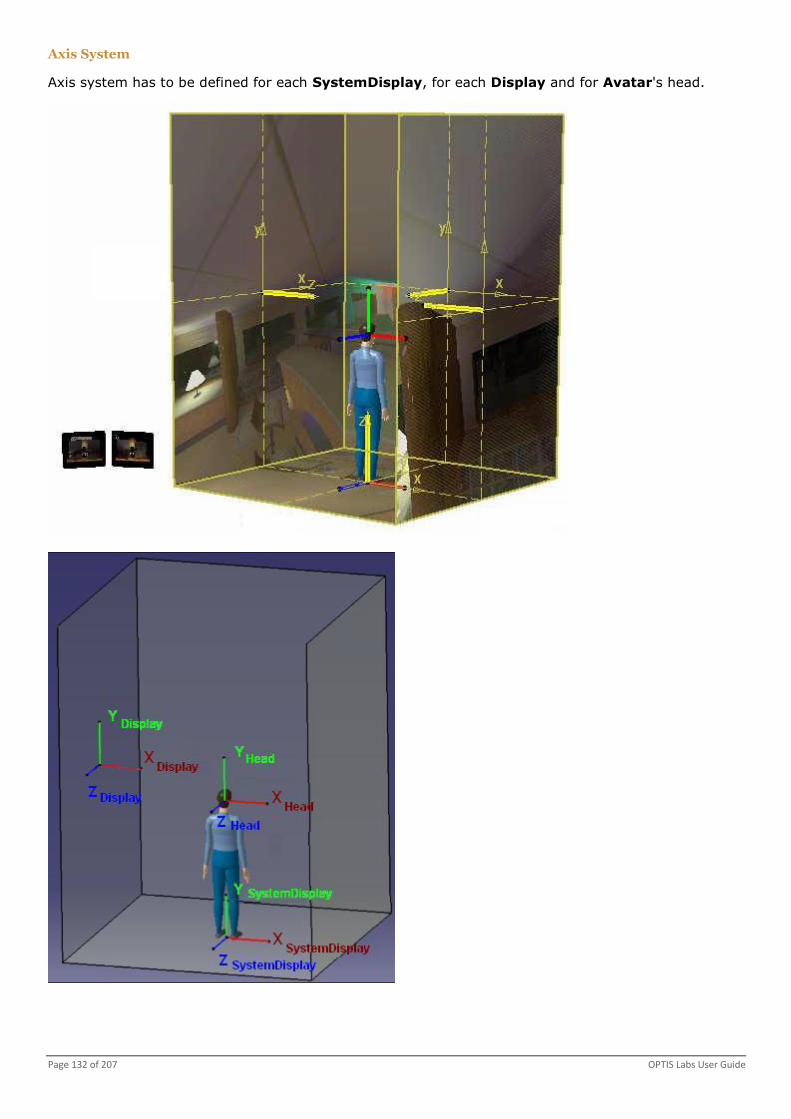
Page 132 of 207 OPTIS Labs User Guide
Axis System
Axis system has to be defined for each SystemDisplay, for each Display and for Avatar's head.
Labs Page 133 of 207
SystemDisplay
Creating a System Display
1. Click the Multiscreen menu, Launch Multiscreen.
A window appears.
2. Click Master Mode.
A window appears.
3. Right-click SystemDisplay and then click Add.
This is the step to define the system in the world.
A window appears.
4. Set the parameters see page 133.
Default values are often kept for the SystemDisplay axis system.
5. Click OK.
The System VR Configuration is updated.
Parameters of a SystemDisplay
The SystemDisplay axis system has to be located in respect of the World axis system.
Position
X, Y and Z positions define the axis system.
Direction
X, Y, Z and Phi directions define the locked direction of the axis system.
Phi is the rotation angle around the defined direction axis.
Display
Creating a Display
A SystemDisplay must be created first.
1. Click the Multiscreen menu, Launch Multiscreen.
A window appears.
2. Click Master Mode.
A window appears.
3. Right-click on All Display and then click Add Display.
A window appears.
4. Set the parameters see page 133.
5. Click OK.
The System VR Configuration is updated.
A mouse move on the icon displays parameters.
Parameters of a Display
The Display axis system has to be located in respect of the SystemDisplay axis system.
Dimension
Xmin, Xmax, Ymin and Ymax dimensions define the size of the Display.
Dimensions of the screen define the center of the screen.

Page 134 of 207 OPTIS Labs User Guide
Position
X, Y and Z positions define the axis system.
It is very important to set an offset to the Display in respect of the SystemDisplay axis system.
Default values should be X=0, Y=0 and Z=-1.
Direction
X, Y, Z and Phi directions define the locked direction of the axis system.
Phi is the rotation angle around the defined direction axis.
The normal of the display is always looking at the center of the SystemDisplay.
Avatar
Creating an Avatar
A SystemDisplay must be created first.
1. Click the Multiscreen menu, Launch Multiscreen.
A window appears.
2. Click Master Mode.
A window appears.
3. Right-click All Avatars and then click Add Avatar.
A window appears.
4. Click AvatarX, Default head and New EyeX to set the parameters see page 134.
Avatar corresponds to the feet position.
5. Click OK.
The System VR Configuration is updated.
Parameters of an Avatar
The axis system of Avatar's head has to be located in respect of the SystemDisplay axis system.
Direction
X, Y, Z and Phi directions define the locked direction of the axis system.
Position
X, Y and Z positions define the axis system.
Avatar's head system has to be offset in respect of the SystemDisplay system.
Window
It is strongly recommended to have one window and several areas to improve calculation
performances.
Creating a Window
You must first define where the zero reference see page 135 is located on your computer screens.
1. Click the Multiscreen menu, Launch Multiscreen.
A window appears.
2. Click Master Mode.
A window appears.

Labs Page 135 of 207
3. Right-click on Windows and then click Add.
A window appears.
4. Set the parameters see page 135.
5. Click OK.
The System VR Configuration is updated.
Parameters of a Window
Definition
X and Y define the window dimensions.
Position
X and Y define the position in reference to your system's origin.
Defining the zero reference
1. Go to Control Panel, Display, Change display settings.
2. Click on the top left corner to check the references.
The zero reference (0,0) is at the top left corner of your main display.
3. Define your system.
Area
An area is included in a window.
Areas and related Display must have the same ratio for the dimensions to avoid image distortion.
All Areas defined from a same computer must have the same dimensions.
In case of several same size Areas, one will be the master Area.
Creating an Area
1. Click the Multiscreen menu, Launch Multiscreen.
A window appears.
2. Click Master Mode.
A window appears.
3. Right-click on Drawing Area and then click Add.
A window appears.
4. Set the parameters see page 135.
5. Click OK.

Page 136 of 207 OPTIS Labs User Guide
The System VR Configuration is updated.
6. Save your complete configuration using the .xml format.
Parameters of an Area
Definition
X and Y define the area dimensions.
Position
X and Y define the position in reference to Windows's origin.
Rendering definition
X and Y define the resolution of the area.
Rendering can not be bigger than the Window dimension.
Less pixels you have, faster the calculation is.
Network Management
Network management has to be set between Master and Slave machines.
Configuring the Network Management
Following steps must be done on master and slaves computers.
1. Click the Multiscreen menu, Launch Multiscreen.
A window appears.
2. Click Network management.
A window appears.
3. Set the parameters see page 137.
4. Click OK.
The configuration is saved in the MultiScreen.cfg file located in the
C:\ProgramData\OPTIS\MultiScreen directory.
To avoid the same modification on all the slaves computers, you can copy this file from the Master
computer to all the Slaves computers at the same location.
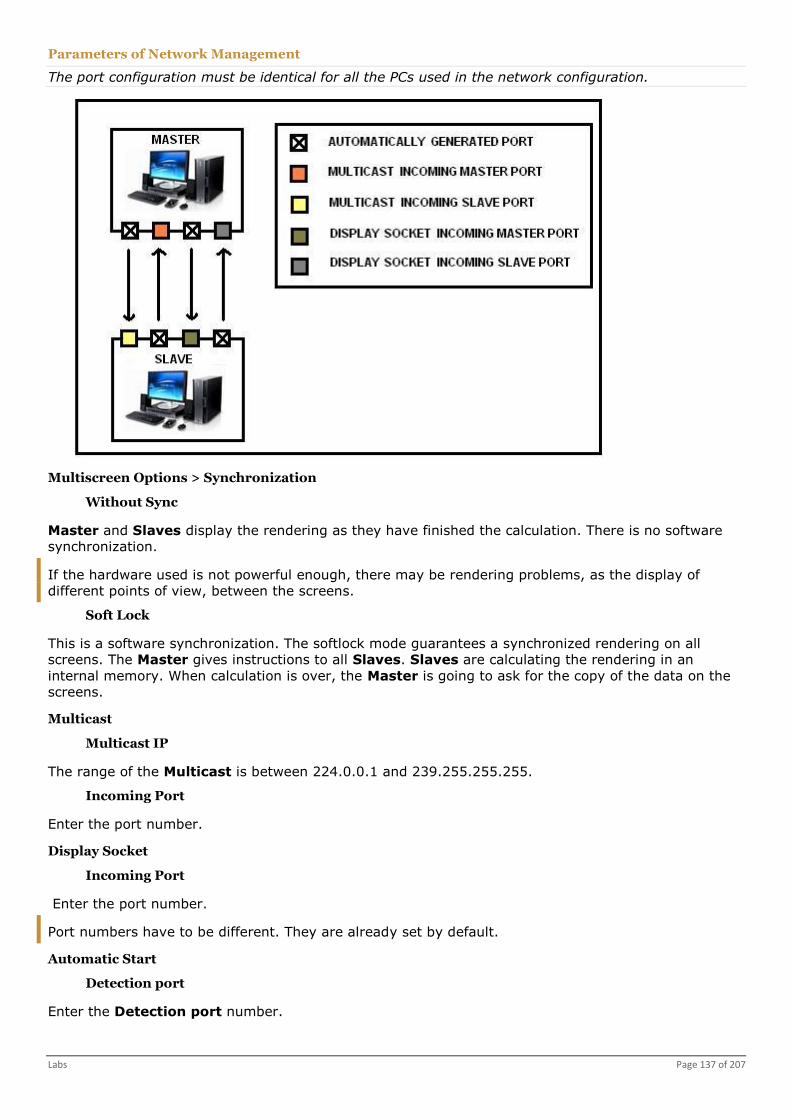
Labs Page 137 of 207
Parameters of Network Management
The port configuration must be identical for all the PCs used in the network configuration.
Multiscreen Options > Synchronization
Without Sync
Master and Slaves display the rendering as they have finished the calculation. There is no software
synchronization.
If the hardware used is not powerful enough, there may be rendering problems, as the display of
different points of view, between the screens.
Soft Lock
This is a software synchronization. The softlock mode guarantees a synchronized rendering on all
screens. The Master gives instructions to all Slaves. Slaves are calculating the rendering in an
internal memory. When calculation is over, the Master is going to ask for the copy of the data on the
screens.
Multicast
Multicast IP
The range of the Multicast is between 224.0.0.1 and 239.255.255.255.
Incoming Port
Enter the port number.
Display Socket
Incoming Port
Enter the port number.
Port numbers have to be different. They are already set by default.
Automatic Start
Detection port
Enter the Detection port number.

Page 138 of 207 OPTIS Labs User Guide
Configuring the Windows Firewall
To enable network communications before using multiscreen with Virtual Reality Lab, configure the
Windows firewall.
1. From the Windows Start menu, select Control Panel.
2. Select Windows Firewall.
3. Click Allow a program or feature through Windows Firewall.
4. Click Allow another program...
5. Click Browse and select OPTIS Daemon.
6. Click Open.
7. Click Network Location Type.
8. Select the the Domain and Home/network (Private) check boxes
9. Click Add.
10. Click Browse and select VRLab.
11. Click Open.
12. Click Network Location type.
13. Select the the Domain and Home/network (Private) check boxes
14. Click Add.
15. Click OK.
Network communications are now fully allowed.
This settings are valid for a basic Windows configuration. If you are encountering further network
communications problems, check you additional firewall and/or antivirus programs.
Cluster
The cluster is for the current machine.
Cluster has to contain at least one Display.
In case of one Avatar with one eye, the eye is defined by default.
It is not possible to overlap windows.
Setting the Cluster for the Master
You must set the network management see page 136 first.
You must have defined a complete configuration see page 130 first.
1. Click the Multiscreen menu, Launch Multiscreen.
2. Click Master Mode.
3. Browse your configuration file.
Cluster window is going to be configured.
If needed, right-click on the Master to Change OpenCL platform.
4. Drag and drop a Window from System VR Configuration window to the Cluster window.
5. Drag and drop an Area from System VR Configuration window to the Cluster window.

Labs Page 139 of 207
6. Drag and drop a Display to [Unlink Display] and Avatar's eyes to [Unlink avatar's eyes].
7. Right-click on Unlink Device and click Link Device.
8. Select the device and click OK.
9. Redo steps for each Area.
10. Save the configuration.
Adding Slaves to the Configuration
In the Multiscreen Distribution window,
1. Click Find slaves.
2. Click Add..., select a computer and click OK.
-Or-
Type a computer name and click Add....
3. Redo previous step for all the slaves you want to add.
If needed you can click Remove to remove a slave computer from the list.
4. Click Find.
Connection can take some time.
New slaves appear in the Cluster area.
5. For each slave computer,
1. Drag and drop a Window from System VR Configuration window to the slave.
2. Drag and drop an Area from System VR Configuration window to the slave.
3. Drag and drop a Display to [Unlink Display] and Avatar's eyes to [Unlink avatar's eyes].
4. Right-click on Unlink Device and click Link Device.
5. Select the platform and click OK.
You can right-click on a slave and click Remove computer to remove a slave from the cluster.
6. Save the configuration.
Starting the MultiScreen Mode
You must have set the cluster for the master see page 138 and the slaves see page 139 first.
1. Click Run.
If you did not save the configuration yet, a message prompts you to save.
A black window appears on each computer of the cluster.
2. From the master, click Open to launch an .OptisVR file.
After a few seconds, the black window on each computer is updated with the .OptisVR image
corresponding to the point of view defined in its configuration.
The download can take some time.
The application automatically runs on slave computers.
In the case there is a distortion of the image you can use a second computer to display it.
From the master, the rendering can be changed to see the effect on slaves.
You can move the mouse to navigate inside the pictures.
3. From the Multiscreen menu, you can click Stop Multiscreen to exit the multiScreen mode.

Page 140 of 207 OPTIS Labs User Guide
Using the Multiscreen Autostart
When you select the Multiscreen Autostart option, the last valid configuration you created is
automatically loaded the next time you launch Virtual Reality Lab.
1. Click the Multiscreen menu.
2. Select Multiscreen Autostart.
The Multiscreen Autostart option is activated.
Using the SIM2 HDR Monitor
You must have a standard monitor for interface and a SIM2 HDR monitor for rendering.
1. From the standard monitor, click Virtual Reality Lab .
The window appears.
The first launch of Virtual Reality Lab can take a while, in this case please wait.
If it is the first time you launch Virtual Reality Lab, the Devices preferences window appears. For
more details, you can view Devices preferences see page 199.
2. Set the Display Monitor see page 194 parameters.
3. Connect the SIM2 HDR monitor using the High Dynamic Range DVI signal connector.
4. From the standard monitor, open the Start menu, click Control Panel, Display, and then select
the Change display settings tab.
1. Select the screen you just added and select the Make this my main display check box.
2. In Multiple displays group box, select Extend these displays.
3. Click OK.
5. In Virtual Reality Lab, click MultiScreen, Launch MultiScreen, then Master Mode.
A window appears.
6. Create the rendering zone on the SIM2 HDR monitor.
To do it, you must create SystemDisplay, Display, Avatar, Window, Area and a Cluster. For
more details, you can view Using Master Mode.
You can start from this .xml (../Common/LAB_OPTIS.zip) file example and personalize it.
You can view the video (../Common/LAB_VRLab_SIM2HDR.zip) if you need more help.
Virtual Reality Peripheral Network
Using Virtual Reality Peripheral Network
1. Click MultiScreen, Launch MultiScreen, then Master Mode.
A window appears.
2. Create the rendering zone.
To do it, you must create SystemDisplay, Display, Avatar, Window, Area and a Cluster. For
more details, you can view Using Master Mode.
You can start from this .xml (../Common/LAB_OPTIS.zip) file example and personalize it.
3. Click Run.
4. Check your VRPN server is connected.
5. Click File, Open or click Open to launch an .OptisVR file.

Labs Page 141 of 207
6. Click MultiScreen, VRPN Configuration.
A window appears.
7. If needed, set your Server Name and Tracker Label.
Server Name can be a name or an IP address.
Tracker Label is your peripheral's name used by your VRPN server.
8. Click MultiScreen, Launch VRPN.
Tracker can be used.
9. Click MultiScreen, Stop VRPN.
Using the Virtual Reality Peripheral Network Autostart
When you select the VRPN Autostart option, the Virtual Reality Peripheral Network is automatically
loaded when you launch Virtual Reality Lab.
1. Click the Multiscreen menu.
2. Select VRPN Autostart.
The VRPN Autostart option is activated.
3D Energy Density Lab
Using 3D Energy Density Lab
1. From Start menu, click All Programs, OPTIS, OPTIS Labs, Labs, 3D Energy Density Lab.
-Or-
1. Click 3D Energy Density Lab .
A window appears.
2. Click File, Open ....
-Or-
Click .
3. Browse a .vmp file.
You can save the VMP map file. In this case you can save your VMP map as a .vmp file.
You can import from txt or export to txt.
You can manage the display see page 142.
Click View, Properties, or , to view properties.
By clicking Filtering, VMP Filtering, you can set a standard filtering.
It only uses neighbors without any considerations regarding values of these neighbors.
In Pass number box, you must type the number of times the filtering algorithm is called. 0 value
means there is no filtering.
The level of filtering is displayed in the status bar of the viewer. By clicking the filter value in the
status bar, you can open the filtering box.
You can make volume and section analysis see page 143.
You can use the Virtual Lighting Controller see page 144.
You can edit preferences see page 145.

Page 142 of 207 OPTIS Labs User Guide
Managing the Display
If you want to move the map, left-click and move the mouse at the same time.
When moving the mouse over the map, values at the position are displayed in the status bar.
If you want to modify the number format, right-click on the status bar.
The number format is the number of decimal per value.
If you want to modify the axis unit of displayed values, right-click on the status bar.
If you want to change displayed colors, use the color list.
Iso levels displays the image with ISO curves or surfaces.
If you want to modify display's parameters, click Tools, Level... or .
You can select a level to modify the value. Press Enter to validate the change.
You can right-click and select Copy to clipboard.
When modifying minimum or maximum value, you can select the Intermediate levels auto-
update check box to compute all intermediate values.
If needed, you can add or delete a color level.
You can click Default to cancel all modifications.
Select the IsoCurve and Filled check boxes, to display the image with or without ISO curves.
Click Linear or Log to switch between a linear or logarithmic scale.
Click Load Scale or Save Scale to load or save parameters in an OPTIS scale file. Format is .scl.
When Iso levels is selected in the color list, you can change the color between two levels clicking
.
Properties
You can select the Decoration check box to display the 3D view tool.
For more details, you can view Using 3D view tool.
You can select the Axis check box, you can display the axis.
You can select the Cutting views check box to display the cutting views.
You can then select the Show Manipulator check box.
Left-click on the axis and move to make a movement.
Left-click on the axis, press Ctrl and move to make a rotation.
Click Up or Down page to change the mode of the used colors.

Labs Page 143 of 207
Volume and Section Analysis
Making Volume and Section Analysis
With Volume and Section Analysis tool, you can have several information inside a volume. You can also
display image section.
1. Click View, Volume....
-Or-
1. Click .
A box appears and a shape appears on your map.
2. Set the parameters see page 143.
3. Close the window.
Parameters of Volume and Section Analysis
Shape
You can select the Parallelepiped type of shape to define the analysis volume.
Center
In Center group box, you must type values to define the position of the analysis volume.
Note that you can use the mouse to set center values.
Direction
In Direction group box, you must type values to define the direction of the analysis volume.
Note that you can use the mouse to set dimensions values.
Dimension
In Dimensions group box, you must type values to define the dimension of the analysis volume.
Note that you can use the mouse to set dimensions values.
Section
You can enable the analysis section. A axis plane is drawn on the map.
If you want to export the map rendering into a XMP file, click Export to XMP.
Sampling
You can change the sampling value.
The sampling is used to improve the definition of the final picture.
Maximum / Minimum
You can read maximum and minimum values of the analysis volume.
You can select the Automatic update check box to compute data in real time.
You can click Update to compute data manually.
You can click Export ... to export in TXT file.

Page 144 of 207 OPTIS Labs User Guide
Virtual Lighting Controller
Using the Virtual Lighting Controller
To use Virtual Lighting Controller, you must have a map with data separated by source, by surface or
sequence (extended or spectral).
With Virtual Lighting Controller, you can change contribution of layers without running new simulation.
Layers can be sources, surfaces or sequence.
1. Click Tools, Virtual Lighting Controller ...
-Or-
1. Click .
A box appears.
2. Set the parameters see page 144.
3. Close the box.
Parameters of the Virtual Lighting Controller
If needed, you can change layers' name.
You can select the Automatic update check box to compute data in real time.
You can click Update to compute data manually.
You can click Select all or Unselect all to respectively select or unselect all the layers.
If needed, you can add or delete a new sliders configuration.
When it is enabled, you can select Power to display power instead of ratio.
In case of spectral map, you can change units using the View menu.
For spectral maps, you can click to display a layer's spectrum.
The option is not available for ambient sources, LCD sources and set of sources including sources
which do not have the same spectrum.
The spectrum change has to be used carefully in case of fluorescent surface.
Vertical lines correspond to the spectral sampling of the xmp.
Click to define a new light source spectrum.
The spectrum of the new source is normalized to get the same power than the initial source. Unit is
photometric or radiometric depending on the one defined in the View menu.

Labs Page 145 of 207
Initial xmp Result after the spectrum change
With , you can delete a spectrum.
This function is only available in the Virtual Photometric Lab, Virtual Human Vision Lab and 3D
Energy Density Lab.
With , you get information a new spectrum has been added.
With , you can get back previous spectrum.
With , you get information a spectral data has not been saved in xmp map.
The spectral sampling of the xmp should be sufficient to cover spectrum of the new layer.
Spectrum of the initial layer should not be null within all spectral zone on each the new spectrum is
not null.
Spectrum changes can take a lot of time because calculations have been made directly on spectral
data of xmp map. When you change a spectrum for the first time, all spectral data are downloaded
in the memory and all modified calculations of layers powers are made on the spectral data. This
can take more time than usual. To avoid this when you do not need any new spectrum change but
only power change, you can clear the View, Load spectral data option.
Editing the Preferences
1. Click Tools, Preferences... .
A window appears.
2. Set the preferences see page 194.

Page 146 of 207 OPTIS Labs User Guide
VIEWERS
Intensity Viewers
Eulumdat Viewer
With Eulumdat Viewer, you can process intensity data stored in Eulumdat file.
Using the Eulumdat Viewer
1. From Start menu, click All Programs, OPTIS, OPTIS Labs, Viewers, Intensity Viewers,
Eulumdat Viewer.
-Or-
1. Click Eulumdat .
A window appears.
You can create, open or save an Eulumdat file. In this case you can save your file as a .ldt file.
When creating an Eulumdat file, you must select the symmetry type.
2. Set the parameters see page 146.
By clicking File, Export ..., you can export an Eulumdat file as a XMP map file. For more details
about XMP map file, you can view Virtual Photometric Lab see page 100.
You can view isolux curves see page 150.
You can display Eulumdat file in two dimensions see page 151.
You can display Eulumdat file in three dimensions see page 151.
You can display Sollner curves see page 152.
Parameters of the Eulumdat Viewer
From General tab, you can set general information about the luminaire.
From Miscellaneous tab, you can set photometric parameters about the luminaire.
Light Output Ratio Luminaire is called LORL.
LORL = Output Flux / Lamp Flux
From Dimensions tab, you can set parameters about luminaire dimensions.
From Symmetry tab, you can set parameters about luminaire symmetry.
It is possible to choose symmetry properties when creating an intensity diagram or to add them on
an existing intensity diagram.
From Lamps tab, you can set lamps that can be used with the luminaire.
When editing the Total Luminous Flux value, the Do you want to preserve (cd/klm) values?
message appears.
The cd/klm unit is used in the Intensity tab.
LORL = Output Flux / Lamp Flux
R = Intensity / Lamp Flux
If clicking Yes, R is constant. If you change the Lamp Flux, the intensity changes proportionally.
LORL is constant. The intensity table and the LORL are not modified.
If clicking No, R is not constant and you keep a constant intensity. If you change the Lamp Flux,
the LORL changes. The intensity table and the LORL are modified.
From Direct ratios tab, you can set direct ratios values for the luminaire.
From Sampling tab, you can read sampling values of C planes and G angles.

Viewers Page 147 of 207
From Intensity tab, you can change intensity values in cd/klm for each sample.
From Luminance tab, you can change luminance values in cd/m².
From Edition tab, you can change options for printing the photometric report.
IESNA LM-63 Viewer
With IESNA LM-63 Viewer, you can process intensity data stored in IES file.
It can be used for all IES formats following the LM - 63 - 95 and previous standards.
Using the IESNA LM-63 Viewer
1. From Start menu, click All Programs, OPTIS, OPTIS Labs, Viewers, Intensity Viewers,
IESNA LM-63 Viewer.
-Or-
1. Click Iesna - LM63 .
A window appears.
You can create, open or save an IES file. In this case you can save your file as an .ies file.
When creating an IES file, you must select the photometric type, the horizontal symmetry and the
vertical angles.
2. Set the parameters see page 147.
By clicking File, Export ..., you can export an IES file as a XMP map file. For more details about
XMP map file, you can view Virtual Photometric Lab see page 100.
You can view isolux curves see page 150.
You can display IES file in two dimensions see page 151.
You can display IES file in three dimensions see page 151.
You can display Sollner curves see page 152.
Parameters of the IESNA LM-63 Viewer
From General tab, you can set general information about the luminaire.
From Tilt tab, you can set information about lamp position and its influence.
If selecting None, tilt has no influence on the lamp output.
If selecting Include, the lamp output varies as a function of the luminaire tilt angle.
You can Add Tilt Angle or Delete Tilt Angle .
In the Lamp to luminaire geometry box, you can select the lamp position in the luminaire.
From Miscellaneous tab, you can set photometric parameters about the luminaire.
In Number of Lamps box, you can type the number of lamps value in the luminaire.
In Lumen per lamp box, you can type the power value of the lamp.
This value is obtained from the manufacturer's technical data. It does not represent the lumens
emitted by the test lamp.
In Candela Multiplier box, you can type the multiplying factor to be applied to all Candela
values in the photometric data file.
In Input Watts box, you can type the consumption value of the lamp.
In Ballast factor box, you can type the Ballast factor value.

Page 148 of 207 OPTIS Labs User Guide
In Futur Use / Ballast lamp photometric factor box, you can type the futur use of the
Ballast lamp photometric factor value.
In the Photometry Type box, you can read the photometric type.
Type C is most of the time used for architecture and roadway. The polar axis coincide with the
vertical axis of the luminaire, and the 0-180° plane contains the luminaire major axis, the length.
Type B is used for adjustable outdoor area and sports lighting luminaire. The polar axis of the
luminaire coincide with the minor axis, the width of the luminaire, and the 0-180 degree
photometric plane coincides with the vertical axis of the luminaire.
Type A, not yet available, is used for automotive headlights. The polar axis coincide with the major
axis, the length of the luminaire., and the 0-180 photometric plane coincide with the vertical axis
of the luminaire.
From Dimensions tab, you can set parameters about luminaire dimensions.
Negative and null parameters give information about the shape.
In Luminous dimensions box, you can change luminous opening dimensions.
In Width box, you can type the distance value in feets across the luminous opening of the
luminaire as measured along the 90-270 axis.
In Length box, you can type the distance value across the luminous opening of the luminaire as
measured along the 0-180 axis.
In Height box, you can type the distance value across the luminous opening of the luminaire as
measured along the vertical axis.
In Units box, you can select Feet to use english units or Meters to use metric units.
In Luminous Shape box, you can read codes about luminous opening shapes (IESNA LM-63-
95):
WIDTH (W) LENGTH
(L) HEIGHT
(H) LUMINOUS SHAPE
0 0 0 Point
w l h Rectangular (default)
-d 0 0 Circular (d = diameter of circle)
-d 0 -d Sphere (d = diameter of sphere)
-d 0 h Vertical cylinder (d = diameter of cylinder)
0 l -d Horizontal cylinder oriented along luminaire
length
w 0 -d Horizontal cylinder oriented along luminaire
width
-w l h Ellipse oriented along luminaire length
w -l h Ellipse oriented along luminaire width
-w l -h Ellipsoid oriented along luminaire length
w -l -h Ellipsoid oriented along luminaire width
From Symmetry tab, you can read parameters about luminaire symmetry.
It is possible to choose symmetry properties when creating a new IES file.
From Data tab, you can set intensity data given in Candela for each sample.
You can Add Vertical Angle , Add Horizontal Angle , Delete Vertical Angle ,
Delete Horizontal Angle .
In Result tab, you can read maximum values for IES files.
Global Maximum is given with its position and Local Maximum for a given horizontal angle.
The IESNA LM-63 viewer gives you its position.
From Luminance tab, you can change luminance values in cd/m² or cd/ft² for each sample.

Viewers Page 149 of 207
From Edition tab, you can change options for printing the photometric report.
OPTIS Intensity Viewer
With OPTIS Intensity Viewer, you can process intensity data stored in Optis intensity file and also
visualize Spectral intensity files in 3D.
Using the OPTIS Intensity Viewer
1. From Start menu, click All Programs, OPTIS, OPTIS Labs, Viewers, Intensity Viewers,
OPTIS Intensity Viewer.
-Or-
1. Click Optis Intensity .
You can create, open, save or import an Optis Intensity file
You can open, save or import a Spectral Intensity file.
When creating an Optis Intensity file, you must select the symmetry.
When opening a file, you can select an Optis intensity file in the .intensity or .int format, or a
Spectral Intensity file in the .spid format.
When saving an Optis Intensity file, you can save your file as a .intensity or .int file.
When importing an Optis Intensity file, you can select a SETFOS file. According to its content, the
SETFOS file is imported as a .intensity or.spid file.
2. Set the parameters see page 149.
By clicking File, Export ..., you can export an Optis Intensity file as a XMP map file. For more
details about XMP map file, you can view Virtual Photometric Lab see page 100.
You can view isolux curves see page 150.
You can display Optis Intensity file in two dimensions see page 151.
You can display Optis Intensity file in three dimensions see page 151.
Parameters of the OPTIS Intensity Viewer
When you open a Spectral Intensity file, you do not have to set theses parameters.
From General tab, you can set a luminaire description.
In Unit box, you must select the photometric or radiometric unit.
In the OPTIS intensity file, the third line corresponds to the unit type.
1 is for photometric units and 0 is for radiometric units.
From Symmetry tab, you can read parameters about luminaire symmetry.
In the OPTIS Intensity file, the fourth line corresponds to the symmetry used in the file:
0: no symmetry,
1: revolution symmetry,
2: symmetry about xOz plane,
3: symmetry about yOz plane,
4: symmetry both about xOz and yOz planes (symmetry in each quadrant).
From Data tab, you can set intensity data given in Candela for each sample.
You can Add Vertical Angle , Add Horizontal Angle , Delete Vertical Angle ,
Delete Horizontal Angle .
From Edition tab, you can change options for printing the photometric report.

Page 150 of 207 OPTIS Labs User Guide
Curves
Isolux Curves
Displaying Isolux Curves
With Isolux Curve, you can view illuminance on a map for a light at a specified height, and isolux
curves at a specified height on a plane.
1. Click View, Isolux Curves.
-Or-
1. Click .
A window appears.
2. Se the parameters see page 150.
By clicking , you can export the isolux curve as a XMP map.
3. Click OK.
Parameters of Isolux Curves
Illuminance Unit gives the result unit.
In Distance box, you can type the distance value in meters between the lamp and the plane or use
the arrows to change it.
In Half map width box, you can type the map size value in meters or use the arrows to change it.
In Levels box, you can type the number of colors in the display or use the arrows to change it.
In Nb of points box, you can type the sampling value or use the arrows to change it.
In Unit group box, you must select the International or the US unit system.
In Display group box, you can select the Grid check box to display the grid.
You must select 2 D to give results as a map, or 3 D to gives results as a 3D shape.
From the Map along list, you must select the plane position.

Viewers Page 151 of 207
Polar Curves
Displaying Polar Curves
With Polar Curves, you can display the intensity data in two dimensions.
1. Click View, Polar Curves.
-Or-
1. Click .
A window appears.
2. Set the parameters see page 151.
3. Click OK.
Parameters of Polar Curves
With Polar Curves, you can display the intensity data in a plane containing the Oz axis, making a
defined C-angle with the xOz plane (C-angle).
In Series group box, you can select Fill check boxes to fill colored curves.
You can select View check boxes to display red or yellow curves that are at +90°.
With the top slider, you can modify the C-angle value for the blue curve of the first series.
With the bottom slider, you can modify the C-angle value for the green curve of the second series.
In Scale group box, you can select the Graduations check box to display graduations.
You can select the Auto scale check box to fit the display.
In Step box, you can type the graduation's sampling value in degrees.
From the Mode list, you must select a polar, cartesian or hybrid display.
From the Unit list, you must select the unit between Candela (cd) or Candela per kilo Lumens
(cd/klm).
You can select the Invert check box to create a top-bottom inversion of the display.
You can select the Link sliders check box to link sliders.
You can select Other distribution to change the distribution with Intensity, IES, Eulumdat, Optis
intensity or TL files.
3D Curve
Displaying 3D Curve
With 3D Curves, you can display the intensity data in three dimensions.
1. Click View, 3D Curve.
-Or-
1. Click .
A window appears.
2. Set the parameters see page 151.
3. Click OK.
Parameters of 3D Curve
You can rotate the image, translate zoom, display a wireframe view.

Page 152 of 207 OPTIS Labs User Guide
Display
You can select the View Shading check box to display a shading view of the intensity envelope.
You can select the View Mesh check box to display the intensity envelope with wireframe.
You can select the Decorations check box to display the 3D view tool.
For more details, you can view Using 3D view tool.
You can select the Axis check box to display the axis.
You can select the Grid OXY, Grid OXZ or Grid OYZ check box to display standard planes grid.
You can select Shape to display the shape.
You can select Color to color.
You can click to display the level.
You can click to set 3D view preferences.
For more details, you can view 3D view see page 196.
Wavelength (nm)
When you open a Spectral Intensity file, the Wavelength (nm) group box appears.
You can use the slider to change the wavelength.
Displaying Sollner Curves
1. Click View, Sollner Curves.
-Or-
1. Click .
Viewers Page 153 of 207
A window appears.
2. Close the window.
Optical Design Viewers
Coupling Efficiency Viewer
The calculation model evaluates the coupling efficiency of a spatial coherent laser beam into a single
mode optical fiber.
This calculation model is included in the laser propagation module within OptisWorks software.
With Coupling Efficiency Viewer, you can evaluate the coupling efficiency by computing the deformation
of the laser beam in phase and amplitude.
This involves to model the real propagation of the electromagnetic field from the laser source to the
fiber, and to compute the overlap integral between the laser input beam and the fiber propagation
field.
The calculation of the incident electromagnetic field in the entrance plane of the fiber is given by the
laser propagation simulation.
An electromagnetic field in form of a sampling matrix of complex numbers is given. For more details,
you can view the OptisWorks User Guide.
Note that the calculation of the electromagnetic field is done in a perpendicular plane to the optical
axis, and this at the observation plane defined by the irradiance sensor.
Using Coupling Efficiency Viewer
1. From Start menu, click All Programs, OPTIS, OPTIS Labs, Viewers, Optical Design Viewers,
Coupling Efficiency Viewer.
A window appears.
2. Click .
A window appears.
3. Set the calculation parameters see page 153.
4. Click OK.
5. Set the parameters to calculate the coupling efficiency see page 155.
You can print the simulation results.
Calculation Parameters
With Calculation Parameters, you can evaluate the fiber mode.
The fiber mode is the transverse distribution function of the electromagnetic field guided by the optical
fiber.
The fiber mode can be defined from each point of the core and the cladding in a given transverse
section.
The field distribution in a transverse section is related to any other transverse sections by a simple
phase shift which depends on the propagation time.
The phase shift factor is
i is the field propagation constant in the optical fiber,
d is the distance between the two transverse sections.

Page 154 of 207 OPTIS Labs User Guide
The mode can be defined as a constant with an undetermined phase.
This undetermined phase does not step in the coupling efficiency but only in the phase shift of the
coupled field.
M(x,y) is the fiber mode in cartesian coordinates.
In Fiber parameters group box, you must select the fiber type.
The fiber mode is automatically calculated.
If selecting Gaussian Fiber, you must type the core index value and the radius value of the
fiber mode in microns.
Radius value is the radius value at 1/e² of energy distribution, or 1/e for the amplitude.
The fiber mode is supposed to be similar to a Gaussian function with a constant phase, equal to
zero.
The gaussian mode can be described by:
Most of the optical fibers respond well to this type of mode.
If selecting Step Index Fiber, you must type the core index value, the cladding index and the
core radius in microns.

Viewers Page 155 of 207
The fiber is defined by step index profile with a symmetric revolution. The step index fiber mode is
defined by the diameter of the core, the core index nc and the cladding index ng.
With these data, you can calculate correctly the fiber mode for the wavelength, under the condition
that such a mode exists.
The mode is determined from the resolution of the Helmotz equation. The result is given by the
following publication.
For more details, you can read Weakly Guiding Fibers : D. Glodge-APPLIED OPTICS/vol10, No
10/October 1971.
Following formula are defined:
a is the radius of the core
k = 2/. is the field propagation constant of the fiber
with nc>>ng
The Helmholtz solutions of the inner and outer field distributions of the core are:
J1 et K1 are the Bessel and Hankel functions of order 1 in cylindrical coordinates
In XMP File box, you can browse the XMP file used for the calculation.
Parameters of Coupling Efficiency Viewer
The calculation of the coupling efficiency needs the correct evaluation of the fiber mode.s
Data
In Data group box, you can type cleavage, tilt and offset values.
Result
In the Efficiency box, you can read the coupling efficiency value in percent.
When calculating the coupling efficiency:
M(x,y) is the fiber mode in cartesian coordinates.

Page 156 of 207 OPTIS Labs User Guide
E(x,y) is the incident electromagnetic field.
The coupling efficiency is the normalized overlap integral of these two functions or, in another way the
normalized scalar product of these two functions.
The M(x,y) and E(x,y) functions are known by the program in form of a matrix of sampled elements.
The form of the numerical approximation of coupling efficiency is given by:
(XF, YF) are the coordinates of the sampled field element (i,j) referred to the center of the fiber.
In Result group box, you must select the calculation mode to calculate the coupling efficiency.
When selecting Fiber / Source, the global coupling efficiency takes into account the
transmission of the optical system.
When selecting Fiber / Beam, the coupling efficiency is the one between the electromagnetic
field of the image space and the fiber mode.
It does not take into account the loss by diffraction, obturation or absorption in the optical system
In Unit box, you must select the unit between Percent and dB.
In Graph group box, you can select a graph.
You can save graphs as .txt or .xls files.
When selecting Tilt X or Tilt Y, you can display the coupling efficiency in function of the tilt
value for the X or Y direction.
The tilt of the fiber is equivalent to a change of the incident angle between the electromagnetic
field and the fiber.

Viewers Page 157 of 207
The incident field of the entrance plane of the fiber is multiplied by the following function:
l and m are the direction cosines in the sense of the x and y axis.
XF and YF are the coordinates in the entrance plane of the fiber.
The tilt of the fiber is a linear phase shift in the incident plane.
When selecting Offset X, Offset Y or Offset Z, you can display the coupling efficiency in
function of the offset value for X, Y or Z direction.
A transverse offset of the fiber in the x or y direction is equivalent to a transverse translation of the
fiber mode of the same quantity, but in the opposite direction.
When selecting Cleavage, you can display the coupling efficiency in function of the distance
from the exit surface to the observation plane.
The display of the graph can take some times because the wave front must be propagated.
The cleavage of the fiber means that the entrance surface of the fiber is not orthogonal to the fiber
axis.
As the same as for the tilt, the cleavage can be expressed by a simple phase shift of the
electromagnetic field.
You can find the field in the plane parallel to the entrance surface.
The phase shift factor is:
nc = core index
The cleavage of the fiber can be compensated by a tilt of the fiber, if the product of the two phase
shift functions is equal to 1.

Page 158 of 207 OPTIS Labs User Guide
By clicking Range, you can type the step number value and the range values used for each
calculation.
Gaussian Propagation Viewer
Using Gaussian Propagation Viewer
1. From Start menu, click All Programs, OPTIS, OPTIS Labs, Viewers, Optical Design Viewers,
Gaussian Propagation Viewer.
A window appears.
2. Open a .txt file.
The simulation results appear see page 158.
You can print the simulation results.
-Or-
1. From the OptisWorks tree, double-click Result manager, Laser results, Gaussian propagation,
and then double-click a .txt file.
The simulation results appear see page 158.
You can print the simulation results.
Parameters of Gaussian Propagation Viewer
You can read parameters of the Gaussian propagation for the source and for the result.
COLUMN DESCRIPTION
W0 (m) Gives the image beam waist diameter at 1/e². The image space is referred as the
space following the refracting surface of this line.
theta (rd) Gives the total beam divergence defined in the current surface material.
rel. pos.
(m)
Gives the position of the "Waist" defined in the current surface material. The
positive direction is the propagation direction of the light.
zr (m) Gives the actual Rayleigh length defined in the current surface material.
E (W) Gives the energy of the beam during the propagation.
F max
(W/m2)
Gives the irradiance in the intermediate material after the surface. It is the power
density in the waist, supposing a global emitted power of 1Watt. The power
density is given in Watts/m². This value has a great importance for the
propagation of a high energy laser beam.
Glass Map Viewer
With Glass Map Viewer, you can apply a particular glass coming from a manufacturer.
Materials contained in the Glass catalog data are available in the manufacturer catalogs.
Using Glass Map Viewer
1. From Start menu, click All Programs, OPTIS, OPTIS Labs, Viewers, Optical Design Viewers,
Glass Map Viewer.
-Or-
1. Click .

Viewers Page 159 of 207
A window appears.
2. Set the parameters see page 159.
3. Click OK.
Parameters of Glass Map Viewer
In the Manufacturer list, you must select a manufacturer name from the list.
Available catalogs are ARCHER, CORNING, HOYA, OHARA, SCHOTT and SUMITA.
In the Glass box, you can select a material coming from glass manufacturers and corresponding
graphs appear.
The red curve is the index in function of the wavelength.
The blue curve is the dispersion in function of the wavelength.
Index is calculated with Sellmeier or Kettler - Helmotz equations belong to the manufacturer.
Sellmeier equation is the following:
Kettler-Helmotz equation is the following:
You can read constringence and dispersion values.
By clicking , you can display the index curve in function of the constringence.
Constringence values are given by the following formula:
nd: material index at 587.6 nm
nc: material index at 656.3 nm
nf: material index at 486.1 nm
By clicking Diagram, Secondary spectrum, or , you can display the dispersion curve in
function of the constringence.
Dispersion values are given by the following formula:
ng: material index at 435.8 nm
nf: material index at 486.1 nm
nc: material index at 656.3 nm
The ABBE line defines normal glass.
Glasses which are not on this line are very interesting to correct chromatism.
By clicking Diagram, Glass Map, or , you can display back the index curve in function of the
constringence
From the Manufacturers box, you can click to clear some manufacturers check boxes.
Only curves corresponding to selected manufacturers are displayed.
By clicking on a specific point, you can view the related values in the Current glass
characteristics box.
If you want to use the zoom, rotate the mouse wheel, click View, Activate zoom or click
and then click on the graph.

Page 160 of 207 OPTIS Labs User Guide
Clicking displays the original size.
When using a large zoom, the glass name is displayed near the point.
Paraxial Data Viewer
Overview
Paraxial Approximation at First Order
Compute paraxial characteristic of an optical system is the first step of optical design to understand
functioning of system and have rough idea of optical performance. Paraxial approximation is a way to
easily and quickly characterize Optical system.
Assumption
Paraxial assumption consists to propagate rays, which remains near optical axis. This assumption
means slope angle, angle of incidence and refraction angle in system approach to zero. Then angle
may be set equal their sines or tangents (first term of Taylor polynomial development):
in radian
One major consequences of this assumption is that trigonometric relation are conveniently transformed
in linear relationship. Rays are fully define by two parameters:
1. slope angle (angle between optical axis and ray),
2. height from optical axis to impact point on surface.
Aperture and Field Ray
This means for optical engineer that every ray passing through diopter has a behavior predictable from
a single linear combination of the two fundamental rays:
1. The aperture ray (AR) (also called marginal ray) starts from the point where object plane intersect
the optical axis (A) and goes through the entrance pupil at on its edge (P), defined by angle u and
height h.
2. The field ray (FR) (also called chief ray or principal ray) starts at the edge of the object-field (B)
and goes through entrance pupil at its center (Q), defined by angle v and height k.
Two cases can be differentiated to set initial aperture and field ray parameters:

Viewers Page 161 of 207
object finite,
Aperture Ray h= 0
u= 1/2 * total angular spread of beam
Field Ray
k= y (height of object)
v= y/x (ratio height of object on distance object
aperture)
object source infinite.
Aperture Ray h= (aperture radius)
u= 0
Field Ray k= 0
v= 1/2 * total field angle
Ray Tracing
The assumption at first order of paraxial rays simplifies greatly any tracing, due to the lack of
trigonometric formula. Any ray (H,U) crossing optical system can be considered as a linear combination
of aperture and field ray.
A coefficient is related to the weight of ray in object field, and B coefficient is related to the weight of
ray in pupil plan.
Knowing this relation, we are able to compute any ray in system, and also to determine by choosing
some specific ray parameters of system, as focal length, image, aperture and focal point localization,
usable pupils diameter.
An abundant literature covers question of paraxial optics and how to compute these paraxials figures.
Paraxial Table
To compute paraxial table is most of optical design first step, due to easiness to fully characterize an
optical system. In this kind of table, quantity h, u', k, v' are computed for each diopter.

Page 162 of 207 OPTIS Labs User Guide
From those first step, other figures are computing as third order aberration.
Primary or Third Order Aberration
Primary aberration is an extension of paraxial theory to higher order of polynomial development. Those
aberrations are related to polynomes of 3rd power. Study of these aberrations provide a first idea of
aberration in system, and can be evaluated with analytical equation.
Then primary aberration has the speed of computation for them, but must be complete with more
accurate aberration study method.
Assumption of Theory
For evaluation of third order aberration, only optical system with a revolution along optical axis are
considered.
We consider an optical system, with an object (AB), with a height of y. We consider ray coming outer
point of object (B), passing through optical aperture (s, and forming an image A'B'. Then aberration
of system can be described as a polynomial development:
This polynomial sum can be greatly simplified by considering assumption made on system:
Ray from object point on axis passing through optical point of lens (intersection of principal plan of
lens and the optical axis) has its image formed along optical axis. Then aberration A0 and B0 terms
are null.
Aberration polynomial of first order are also null, if we consider A'B' as paraxial image. Then linear
terms are just magnification of optical system.
In an axially symmetrical system, it can not have even order polynomial aberration, only odd order.
Then aberration development can be re-written as:
First aberrations, to appear in an axially symmetrical system, have power of third order. Then this
aberrations are named primary aberration or Third-order aberration.
In polynomial decomposition of aberration, higher the order of aberration is and smaller its effect will
be. Then to optimize an optical system, always smaller order must be minimized first.
Primary Aberration
Primary aberrations have been studied and classified for monochromatic light, by Ludwig Von Seidel
(1821-1896) in the 1850th. He determined that it exists only five primary aberrations and that they
could be computed with a combination of five polynomials :
Spherical aberration can be defined as focus variation with system aperture. This aberration
come from that an axial ray on edge of pupil are brought to focus faster than paraxial focus.
It exist the longitudinal (or axial) spheric aberration, which characterizes distance between paraxial
focus to an axial ray focus.
Spheric aberration can be described by its transverse magnitude. This value is called transverse.
This is distance, of an axial ray focus position from optical axis at paraxial focus plan position.

Viewers Page 163 of 207
In order to characterize maximum incidence on image of spherical aberration, transverse and
longitudinal aberration are given for margin ray of optical system.
Coma can be defined as magnification variation with system aperture.
Tangential coma is distance between point image of ray through the center of lens to point image
of upper and lower ray.
Image of point has appearance of a comet shape flare. Aberration names comes from this
particular shape.
Coma as far as it depends of field incident angle, coma aberration are evaluated at maximum
incident angle.
Curvature aberration can be defined as curvature of plan in order to have best focus point (or
least diffusion circle).
Curvature as far as it depends of field incident angle, curvature is estimated with maximum
incident angle.
Astigmatism aberration can be defined as best focus variation in function ray position on sagital
and tangential axis.
Astigmatism tangential or sagital is distance between least diffusion circle position and respectively
tangential or sagital focus point.

Page 164 of 207 OPTIS Labs User Guide
Astigmatisms are related to incident angle, then tangential and sagital astigmatism are computed
for maximum incident angle.
Distortion (D) can be defined as magnitude as displacement of image compared expected image
with paraxial calculation.
A regular square grid is deformed in pincushion when distortion has a value positive and barrel
when distortion has a negative value.
On left, image has a positive distortion (or pincushion), and right picture represents its opposite: a
negative distortion (or barrel).
Using Paraxial Data Viewer
1. From Start menu, click All Programs, OPTIS, OPTIS Labs, Viewers, Optical Design Viewers,
Paraxial Data Viewer.
A window appears.
2. Open a .txt file.
Viewers Page 165 of 207
The simulation results appear see page 165.
You can print the simulation results.
-Or-
1. From the OptisWorks tree, double-click Result manager, Optical results, Paraxial, and then
double-click a .txt file.
The simulation results appear see page 165.
You can print the simulation results.
You can click to calculate a Seidel sums.
Parameters of Paraxial Data Viewer
Wavelength
On Wavelength list, you can choose wavelength according to wavelength chosen in optical source.
Be careful to set correctly wavelength. Results in Paraxial table and Aberration of third order results
depends of wavelength considered.
Paraxial Table (First-order propagation)
Focal Length
Focal length value is computed by considering propagation of an input parallel ray to optical axis
(H=1, U=0), through diopters. Focal Length is distance between image principal plane and image
focal plane.
Focal length, in paraxial table, is given for an output surface (index i). Focal Length index i is the
effective focal length of the optical system from the its first diopter to its surfaces index i.
HeightA, AngleA,
These values refer to aperture ray traced through optical system from its first diopter and up to surface
index i.
HeightA is the height of aperture ray on surface i.
AngleA is the output angle of aperture ray on surface i.
HeightF, AngleF
These values refer to field ray (chief ray) traced through optical system from its first diopter and up to
surface index i.
HeightF is the height of chief ray on surface i.
AngleF is the output angle of chief ray on surface i.
Back Focal Length (BFL)
Back Focal Length (BFL) of an optical system is distance between the output surface of system to
focal point of system.
Back Focal Length, in paraxial table, is given for an output surface index i of system. Then BFL is
distance from output surface index i to focal point of optical system build considering diopter up to i
surface.
Seidel Coefficient
Click to display Seidel coefficients.
Coefficient display in Seidel windows are:

Page 166 of 207 OPTIS Labs User Guide
The fifth Seidel polynomials,
The contribution of the fifth primary aberration.
General expression of primary aberration is:
Primary aberrations are computed with Seidel polynomials. These relations are called Nijboer relations.
Lateral Spherical Aberration (S.A. lateral)
The lateral (or transversal) spherical aberration is computed with the first Seidel sum, according to
relation:
Axial Spherical Aberration (S.A. axial)
The axial (or longitudinal) spherical aberration is computed with the first Seidel sum, according to
relation:
Coma
Coma radius is related to second Seidel term.
Sagital Astigmatism (Delta Sag.)
Given by equation :
Tangential Astigmatism (Delta Tan.)
Given by equation :
Distortion
where SIII and SIV are the third and fourth sums of SEIDEL.
The displacement of the size of the image:
Distortion is displacement of image, related :
The distortion is in %:
l is the invariant of Lagrange.

Viewers Page 167 of 207
Real Aberrations Coefficients Viewer
Using Real Aberrations Coefficients Viewer
1. From Start menu, click All Programs, OPTIS, OPTIS Labs, Viewers, Optical Design Viewers,
Real Aberrations Coefficients Viewer.
A window appears.
2. Open a .txt file.
The simulation results appear see page 167.
You can print the simulation results.
-Or-
1. From the OptisWorks tree, double-click Result manager, Optical results, Aberrations,
Aberrations coefficients, and then double-click a .txt file.
The simulation results appear see page 167.
You can print the simulation results.
Parameters of an Aberration Coefficient Calculation
The real aberrations tab represents the same information than real aberrations graph.
For more details, you can view Real Aberrations Viewer.
The numerical aberration values are displayed in millimeters.
Eight families appear:
TRANSVERSAL COMA ASYMMETRY SYMMETRY
SAGITTAL CURVATURE ASTIGMATIS
M
DISTORTIO
N
Each function is characterized by the object position in the field and the intersection point in the
entrance pupil plane.
All the positions are expressed as normalized fractions of the total field and the total aperture:
central 0.0 the object point is situated on the optical axis
zonal 0.7 the object point is fixed at 0.7 of the total
field-of-view
marginal 1.0 the object point is fixed at the edge of the
field-of-view.
Knowing the significance ofzonal(Z) and ofmarginal(M) simplifies the association between the
aberration and its abbreviation.
Transverse aberrations TAM and TAZ.
y' is the intersection point of the ray in the image plane.
y'0 is the height of the ray passing through the center of the entrance pupil.
y'1 is the height of the ray passing through the entrance pupil at 0.7 of the pupil height.

Page 168 of 207 OPTIS Labs User Guide
y'2 is the height of the ray passing through the entrance pupil at the edge.
We use these points to define the following functions:
TAM = y'2 - y'0 TAZ = y'1 - y'0
Coma near the optical axes, COMAM and COMAZ.
y' is the paraxial image height of an object of height y. y'1 is the height of the ray from the object
centre to the edge of the pupil.
y''1 is the height of the ray from y passing the edge of the pupil.
We use these points to define the following functions.
The COMAZ function is exactly the same as COMAM with the ray passing at 0.7 of the pupil height.
Asymmetry and Symmetry
Ray at the Edge of the Pupil
Given the three rays from the point in the field passing through the centre and two edges of the pupil
we obtain the three intersections y'0, y'1 and y'3.
At the Field Edge: AEM and SEM
The asymmetry of the field is termed AEM and is defined as: AEM =
The symmetry at the field edge SEM is defined as: SEM =
At 0.7 of the Field (Zonal Field) AZM and SZM
The definition of AZM and SZM follow the same principle as the previous aberration but the rays start
from 0.7 of the total field. The asymmetry in the zonal field is termed AZM and is defined as: AZM =
Similarly we define the symmetry in the zonal field (SZM) as: SZM =

Viewers Page 169 of 207
Ray at 0.7 of the Pupil Height
Given three rays defined by the starting point in the field and passing the center of the pupil and the +
and - 0.7 pupil heights, we obtain the three impact points y'0, y'3 and y'4.
At Edge of Field: AEZ and SEZ
The asymmetry at the edge of the field is termed AEZ and is defined as: AEZ =
Then we define the symmetry at the edge of the field by the function SEZ: SEZ =
At 0.7 of the Field (Zonal Field) AZZ and SZZ
The AZZ and SZZ functions are exactly the same as AEZ and SEZ with the ray starting from 0.7 of the
total field. The asymmetry in the zonal field is termed AZZ and is defined as: AZZ =
Then we define the symmetry in the zonal field as: SZZ =
Sagittal Aberrations
The Sagittal aberrations are defined by moving the object from the y axis and also moving the
intersection point in the pupil from the x axis.
We obtain an intersection point with the coordinates (x',y').
The x' value allows us to define the following functions: XEM = x' for the edge of the field and the edge
of the pupil XEZ = x' for the edge of the field and 0.7 of the pupil height. for the zonal filed and the
pupil edge XZZ = x' XZM = x' for the zonal field and 0.7 of the pupil height.
Distortion
y' is the image of the paraxial object y.
y' is the intersection of the field ray with the image plane.

Page 170 of 207 OPTIS Labs User Guide
Distortion values are : Marginal Distortion: for DISTM = y'1-y the total field Zonal Distortion: for DISTZ
= y'1-y 0.7 of the total field.
Astigmatism and Curvature
Astigmatism and curvature functions are defined by variations of the field ray. The variations are made
at the pupil. Variations in dy give the tangential functions and variations in dx give the sagittal
functions.
Tangential Field Curvature
This is defined by a variation dy across the pupil. These functions are defined by:
Edge of field: TFCM =
At 0.7 of field height: TFCZ =
Sagittal Field Curvature
This is defined by a variation in dx across the pupil. The functions are defined as:
Edge of field: SFCM =
At 0.7 of the field: SFCZ =
Astigmatism
The astigmatism functions are defined by the difference of TFC and SFC. We obtain the expression:
ASTM = TFCM - SFCM ASTZ = TFCZ - SFCZ
Conclusion
Each of the these functions gives important information about the optical system quality based on the
specified criteria. These definitions are essential to evaluate the performances of the optical system.
Real Aberrations Viewer
Using Real Aberrations Viewer
1. From Start menu, click All Programs, OPTIS, OPTIS Labs, Viewers, Optical Design Viewers,
Real Aberrations Viewer.
A window appears.
2. Open a .txt file.
The simulation results appear see page 171.
You can print the simulation results.
-Or-

Viewers Page 171 of 207
1. From the OptisWorks tree, double-click Result manager, Optical results, Aberrations,
Aberrations, and then double-click a .txt file.
The simulation results appear see page 171.
You can print the simulation results.
Parameters of Transverse Ray Aberrations Viewer
Overview
Transverse ray aberration viewer shows ray aberration as function of pupil coordinate.
X' component of transverse ray aberration in function of X position on pupil are build by launching a
fan ray along X-axis (sagital ray). Y’ transverse aberration contribution are computed by launching a
ray fan along Y-axis.
The plotted data is the distance between the ray intercept coordinate and the chief ray intercept
coordinate. Plotted data in graph are function of ray position pupil. If many wavelengths are selected,
then each plot is referenced to their chief ray position.
Axis definition :
The horizontal axis for each graph represents the normalized and oriented entrance of pupil
coordinate (1 represents the total radius of the pupil).
The vertical axis scale is given at the right side of viewer, and are expressed in µm.
Field
Field list allows to select the percentage of field from which the plotted data are calculated.
Automatic Window Size
Diagram is auto-scale in order to visualize fully plotted data, no matter what the selected field is. An
option is provided in order to scale manually spot diagram:
1. Click to clear Automatic window size.
2. Enter the scale in microns of the plot (Value max - value min) in the scale box.
3. Click Update to apply new scale.

Page 172 of 207 OPTIS Labs User Guide
Spot Diagram Viewer
Using Spot Diagram Viewer
1. From Start menu, click All Programs, OPTIS, OPTIS Labs, Viewers, Optical Design Viewers,
Spot Diagram Viewer.
A window appears.
2. Open a .ray file.
The simulation results appear see page 172.
You can print the simulation results.
-Or-
1. From the OptisWorks tree, double-click Result manager, Optical results, Spot Diagram, and
then double-click a .ray file.
The simulation results appear see page 172.
You can print the simulation results.
Parameters of Spot Diagram Viewer
The spot diagram gives the position (x, y) of the various ray impacts in an analysis plane defined by its
position z on propagation axis.
Wavelength
In the Wavelength list, you can select or unselect Wavelength ALL to see the impacts of the image
spot or just the impacts from one selected wavelength, which expressed in nanometers (nm).
Field
With the Field list, you can center spot diagram on image spot of selected percentage field.
Automatic Window Size
Diagram is auto-scale in order to visualize all ray impact of selected field in same window.
An option is provided in order to scale manually spot diagram.
You must click to clear the Automatic window size check box, in the Scale box, you must type the
amplitude value in µm spot of diagram full scale (Value Max. -Value Min.), and then you must click
Update to apply new scale.
Best Focus
Energy
The proportion of ray impacts to consider best focus search.
100% means that all ray are taken into account.
80% means that calculus take in account 80 % impacts ray from all, which have the smaller radius.
RMS /GEO
With the RMS/GEO list, you can set method used in order to look for best focus.
If you click RMS, the best focus radius is evaluated with the root mean square of all impact radius
from middle point.
If you click GEO, the best focus radius is evaluated with the average of impact radius. In this
method only impacts with smaller impact radius is taken into account. Proportion of impacts to take
in account is set in field Energy.

Viewers Page 173 of 207
Local Best Focus
If you click Local Best Focus, the viewer looks for position on propagation axis which minimizes spot
radius for selected field.
In case of a multi-wavelength spot diagram, if Wavelength ALL is selected, Local Best Focus is
equal to the barycenter of the Local Best Focus from each wavelengths regarding the wavelengths’
weights from the optical source definition.
Spot diagram is updated in order to display the best local spot. Then analysis plan position is offset
along optical axis according to distance find with Local Best Focus algorithm.
Global Best Focus
If you click Global Best Focus, the viewer looks for position on propagation axis and considering all
fields. Global Best Focus is equal of barycenter of the Local Best Focus from each fields regarding the
fields’ weights from the optical source definition and taking the same selected wavelengthIn case of a
multi-wavelength spot diagram, Global Best Focus minimizes spot diagram radius without taking into
account wavelength. All spot impact are bundle, without prior consideration of wavelength.
Spot diagram is updated in order to display the best global spot. Then analysis plan position is offset
along optical axis according to distance find with Global Best Focus algorithm.
Sensor Offset
Position
Position value is the offset applied to analysis plan position from initial detector position set in CAD,
along propagation axis of the system.
Step
You can check evolution of spot diagram along propagation axis. Step value is the offset applied from
previous position for each click.
Upper arrow shifts sensor of Step value toward higher Z position value (detector goes further from
optical system).
Bottom arrow shifts sensor of Step value toward lower Z position value (detector comes further
from optical system)
Spot Data
Center X
It is x coordinate of spot diagram middle point. Middle point is the mean of x-coordinate maximum and
x-coordinate minimum. If you selected Wavelength ALL, all impacts without wavelength restriction,
are considered to calculate Center X.
This value is used to center spot diagram.
Center Y
It is y coordinate of spot diagram middle point. Middle point is the mean of y-coordinate maximum and
y-coordinate minimum. If you selected Wavelength ALL, all impacts without wavelength restriction,
are considered to calculate Center Y.
This value is used to center spot diagram.
RMS radius
RMS radius is the root of mean of the square radius of all ray impact for selected field. RMS radius is
computed by considering a circle centered on middle point. If you selected Wavelength ALL, all
impacts without wavelength restriction, are considered to calculate RMS radius.
GEO radius
This value is radius in order to encircled of all ray impact for selected field. GEO radius is computed by
considering a circle centered on middle point. If you selected Wavelength ALL, all impacts without
wavelength restriction, are considered to calculate GEO radius.

Page 174 of 207 OPTIS Labs User Guide
Airy Radius
This value is the radius of diffraction spot. This is the minimal spot radius that we can reach in an
optical system.
If you selected Wavelength ALL, this value is computed for the barycenter of the wavelengths
regarding their weights from the optical source definition.
Geometric MTF
Frequency X
Frequency X is the spatial frequency in which Geometric MTF drops to 20% for first time along X-axis.
Frequency Y
Frequency Y is the spatial frequency in which Geometric MTF drops to 20% for first time along Y-axis.
GEO Radius VS Disfocusing Viewer
Click to display GEO Radius VS Disfocusing curve.
This is the radius computed which is encircled 100% along optical propagation axis.
Axis definition:
X-axis : offset of sensor position from current position displayed in spot diagram. Then zero
position correspond to current sensor position in spot diagram. Sensor position is express in
millimeters.
Y-axis : GEO Radius displayed in µm.
GEO radius is computed with middle point of Spot and considering number of ray impact.
If you selected Wavelength ALL, all impacts are bundle, without prior consideration of
wavelength.
Encircled Energy Viewer
Click to display Encircled Energy curve.
This viewer displays radius in function of encircled energy proportion considered. For example, in curve
below, there is 80% of Energy in a circle with a radius about 130µm.
Axis definition:
X-axis : Proportion of Encircled Energy.
Y-axis : Radius in which proportion of energy is encircled.
Radius of Encircled Energy is computed with middle point of Spot and considering number of ray
impact.
If you selected Wavelength ALL, all impacts are bundle, without prior consideration of
wavelength.

Viewers Page 175 of 207
Geometric MTF viewer
Click to display Geometric Viewer.
The Modulation Transfer Function MTF is image contrast of light and dark bars test chart in function
of object spatial frequency. This test chart is composed by equally spaced light and dark bars, which
follow a sines relation. Pitch (or spatial frequency) between light and dark bars is expressed a certain
number of lines per millimeter.
MTF gives contrast response against frequency to a spatial stimulation . As far as optical systems have
aberrations, line image will tend to mix with the other nearest lines images. Then lines images will tend
to blur according to pitch between them. This function then allow to discern limit of resolution.
MTF is time to time referred as frequency response or sine wave response or contrast transfer
function.
MTF plot against frequency is thus an universal measurement of optical performance, which could be
applied on a great amount of optical systems: image-forming, lenses, films, camera... One convenient
characteristic of MTF is that MTF of optical combination can be calculated by multiplying MTF of each
component.
As far as you use geometrical ray propagation to compute MTF, GEO MTF is only valid is if spot radius
is bigger to 10 times of the Airy radius.
Axis definition:
X-axis : spatial frequency expressed in number of lines per millimeter.
Y-axis : Contrast figure.
Curves legend:
Curve with blue cross is the MTF computed by considering only diffraction aberration. This curve
is the theorical performance of an optical system. On example above, this curve is on top of graph.
Curve with green dots is MTF computed with spot spread function along X-axis.
Curve with blue dots is MTF computed with spot spread function along Y-axis.
If you selected Wavelength ALL, MTF due to diffraction (curve with blue cross) is evaluated by
taking the barycenter of the wavelengths regarding their weights from the optical source definition.
If you selected Wavelength ALL, each impact is bundled regarding its wavelength’s weight from
the optical source.

Page 176 of 207 OPTIS Labs User Guide
RAY FILE TOOLS
Source Generator
With the Source Generator, you can create .ray files for different type of sources.
Using the Source Generator
1. From Start menu, click All Programs, OPTIS, OPTIS Labs, Ray File Tools, Source Generator.
A window appears.
You can edit, load or save a source. In this case you can save your source as a .sou file.
2. Select the source type you want to create.
A window appears.
3. Set the parameters see page 176.
4. If needed click Position/Orientation.
Some sources, such as the arc lamp, can be translated and rotated.
A window appears.
5. Set the parameters see page 183.
6. Click OK.
If needed, you can select Save Rays to load light rays (.ray file).
Parameters
Parameters of Optical Fiber
Geometry/Fiber Type
By selecting Step index fiber, a disk with a uniform spatial radiant exitance distribution
approximates the source.
The diameter for the disk is defined as the fiber core diameter.
The angular distribution is a Gaussian distribution.
The half angle q of the divergence at 1/e² is given by: sin(q)=NA
NA is also known as the numeric aperture of the fiber.
By selecting Gradient index fiber (gaussian), a disk approximates the source with a Gaussian
distribution for the radiant exitance.
The diameter at 1/e² is defined as the fiber diameter.
The angular far field distribution is also a Gaussian distribution.
The half angle q of divergence at 1/e² is defined as: sin(q)=NA
NA is also known as the numeric aperture of the fiber.
By selecting Gradient index fiber (quadratic), the source is approximated by a rectangle with a
Gaussian distribution for the radiant exitance.
The definition is similar to the one above.
Emittance
In the Diameter at 1/e² of box, you can type a diameter value in microns.

Ray File Tools Page 177 of 207
Intensity
In the Sine of half angle of box, you can type a sine value.
Energy
In the Radiant flux in box, you can type the radiant flux value in Watt.
Spectral Range
In Spectral Range group box, you can click Spectrum.
For more details, you can view Parameters of Spectrum see page 183.
Parameters of LED
A disk having an uniform emittance approximates the source.
A Gaussian distribution approximates the intensity distribution.
This model may be used as a first approximation to simulate a LED with a collimating optical system.
But there is also a more accurate way to simulate the LED where a more explicit description of the far
and near fields is needed.
The LED should thus be modeled as a Lambertian emitter and the collimating system can then be
directly entered in the editor.
The example file LED.SOP is an explicit simulation of a Light Emitting Diode by a Lambertian source
with the collimating optical system.
The Lambertian source enables you to take into account the emittance variation of the emitting surface
of the LED.
For more details about the Lambertian source, you can view Parameters of Lambertian Source see
page 178.
The radius and the distance from the Lambertian source to the lens surface can be found in the
technical documentation of the LED.
Emittance
In the Beam Diameter at 1/e² box, you can type a beam diameter value in millimeters.
Intensity
In the Total angle divergence at 1/e² box, you can type a total angle value in degrees.
Energy
In the Radiant flux in box, you can type the radiant flux value in Watt.
Spectral Range
In Spectral Range group box, you can click Spectrum.
For more details, you can view Parameters of Spectrum see page 183.

Page 178 of 207 OPTIS Labs User Guide
Parameters of Lambertian Source
A Lambertian surface is such that the intensity of the light emitting surface in a given direction is
proportional to the cosine of the normal's angle to the surface.
The brightness (luminance, radiance) of a Lambertian surface is constant regardless of the angle from
which it is viewed.
Geometry
The Lambertian source is a flat source which can have a rectangular or elliptical shape.
In Geometry box, you can select Ellipse or Rectangle.
You must type the Size X and Size Y values in millimeters.
The emittance distribution is uniform. If you want to simulate non uniform emittance distribution, refer
to the user defined sources.
For more details, you can view Parameters of User Defined Source see page 180.
Intensity
The intensity distribution is always Lambertian which means proportional to the cosine of the normal
angle of the surface.
In the Half-angle of emission box, you can type a half-angle of emission value in degrees.
Within the emission angle, rays are emitted and no rays are emitted beyond this limit angle of
emission.
The advantage of the definition of the emission angle is a speed gain in the computation time: why
should a ray be emitted in a direction where they are absorbed in any case.
Energy
In the Radiant flux in box, you can type the radiant flux value in Watt.
The energy value fixes the radiation flux emitted in the cone defined by the emission angle.
Spectral Range
In Spectral Range group box, you can click Spectrum.
For more details, you can view Parameters of Spectrum see page 183.

Ray File Tools Page 179 of 207
Parameters of Multimodal Laser Diode
Geometry
The source is represented by a flat rectangle which may have different dimensions in the x and y
directions.
In Waist Diameter in X and Waist Diameter in Y boxes, you must type values in millimeters.
Emittance
The emittance distribution is either uniform or Gaussian in the x and y directions.
Both directions may have different distributions.
In Emittance boxes, you must select gaussian or uniform.
Intensity
The angular distribution is always Gaussian.
You must type the total divergence angle values of the Gaussian curve at 1/e² of its maximal intensity
value.
The divergence angle may be different for the x and y directions.
Energy
In the Radiant flux in box, you can type the radiant flux value in Watt.
Spectral Range
In Spectral Range group box, you can click Spectrum.
For more details, you can view Parameters of Spectrum see page 183.
Parameters of Black Body
A Black Body is an object which does not reflect any electromagnetic radiations at any wavelength.
The radiance from a black body is the radiance from a system in thermodynamic balance, defined by
its temperature.
This source is a particular case of a Lambertian source and is characterized by its temperature and
shape.
This source model is suitable for most thermal sources.
The black body is totally defined by following parameters concerning its spectral distribution and the
emitted radiation flux.
Geometry
In Geometry group box, you must select ellipse or rectangular, and you must type size values in
millimeters to define the extension in both directions.
Emittance
The emittance is uniform.
Intensity
The intensity distribution is Lambertian.
The half angle of emission fixes the angle in which the rays are emitted

Page 180 of 207 OPTIS Labs User Guide
You must type the half angle of emission value in degrees.
Energy
In the Energy group box, you can type the temperature and emissivity values.
The energy emitted by a black body is defined by its temperature and its emissivity. A perfect black
body has an emissivity of 1.
Lambda max is the Lambda maximum of the emitted spectrum.
The wavelength is for which the spectral emittance is maximal.
The wavelength may be calculated by Wien's Displacement Law in the following way:
lmax = k1 / T
with k1 = 2898 mm.K
where T is the temperature in Kelvins
Total power and used power are the radiation emitted in 2p (half space) which is given for the
chosen spectral range and for all wavelengths from the defined black body.
The indicated values take care of the emissivity.
The used power indicates the amount of radiation effectively emitted in the cone defined by the
half angle of emission.
The radiation values are calculated by Plank's Radiation Law and by the Stefan-Boltzmann's Law.
Spectral Range
The spectral distribution is defined only by the temperature.
In Spectral Range group box, you can type the Lambda and number of samples values.
Lambda min is the Lambda min which define the smallest wavelength of the spectral range used for
the simulation.
Lambda maxis the Lambda max which set the longest wavelength of the spectral range.
Number of samples sets the number of samples used for the simulation.
The maximal number of wavelength samples is 100.
Parameters of User Defined Source
Light sources are very often defined by their physical and geometrical characteristics.
The intensity distribution as well as the emittance distribution are defined by a limited number of
general parameters.
With user defined sources, you can define the source characteristics (emittance and intensity
distribution) by numerical distribution.
You can define non-symmetrical sources or sources, which have characteristics, which are not covered
by the other more generally defined sources.
An increase in the computing time is a consequence of the more general definition possibilities.
In order to optimize an optical system for photometric performances, you should use the basic and
faster source models first.
Only the final step in optimization should be done with the user defined source model.
Another possibility is to use the Saved Rays option to save computing time.
Geometry/Emittance
In Geometry/Emittance group box, you must select a geometry for the source, which defines the
near field.
Intensity
In Intensity box, you must select the intensity distribution (the far field) characteristics of the light
source.

Ray File Tools Page 181 of 207
Each intensity distribution may be combined with any of the geometries presented here.
Energy
In the Radiant flux in box, you can type the radiant flux value in Watt.
The radiant flux represents the flux which is emitted in the angle defined by the intensity distribution.
Spectral Range
In Spectral Range group box, you can click Spectrum.
For more details, you can view Parameters of Spectrum see page 183.
Parameters of Incandescent Lamp
With the incandescent lamp, you can define the same shapes/volumes of extended sources.
An incandescent lamp emits light when an electric current passes through a filament, which is situated
in a vacuum tube.
Rays are emitted from the surface.
The surface emission determines the far and near field characteristics of the lamp according to the
shape of the wire.
The spectral distribution is the distribution of a black body given by the wire temperature.
Geometry
The geometry of the lamp is defined in a special geometry editor.
Emittance
In the Half-angle of emission box, you can type a value in degrees.
The emission angle is the angle between the optical axis and the maximal emission direction of the
rays.
No ray is emitted in a direction outside of the cone defined by the half angle of emission.
Furthermore, the radiation flux is related to this cone: all radiation flux will be emitted in this cone.
Energy
In the Radiant flux in box, you can type the radiant flux value in Watt.
The radiation flux is defined in radiometric units and then automatically translated into photometric
units.
Spectral Range
In Spectral Range group box, you can type the Lambda, number of samples and temperature values.
The spectral distribution is the distribution of a black body at a defined temperature.
The spectral range is then fixed by the maximal and the minimal wavelengths.
The number of samples fixes the sampling rate for the spectral distribution.
The spectral distribution of a black body is only a suggested distribution, which satisfies a huge number
of applications.
Nevertheless, the user can redefine the spectral range as well as the spectral distribution.
For more details, you can view Parameters of Spectrum see page 183.
Page 182 of 207 OPTIS Labs User Guide
Parameters of Fluorescent Lamp
A Fluorescent lamp is for instance, a tube containing mercury vapor and lined with phosphor. When a
current passes through the gas, visible light is emitted from the vapor.
In consequence, the rays are emitted from the volume and not only from the surface, as is the case for
incandescent lamps.
The volume emission determines the emission characteristics of the light source according to the shape
of the tube.
Geometry
The geometry of the lamp is defined in a special geometry editor.
Emittance
In the Half-angle of emission box, you can type a value in degrees.
The emission angle is the angle between the optical axis and the maximal emission direction of the
rays.
No ray is emitted outside of the cone defined by the half angle of emission.
Furthermore, the radiation flux is related to this cone: all radiation flux will be emitted in this cone.
Energy
In the Radiant flux in box, you can type the radiant flux value in Watt.
Spectral Range
In Spectral Range group box, you can click Spectrum.
The spectral distribution depends on the gas used in the tube.
For more details, you can view Parameters of Spectrum see page 183.
Parameters of Arc Lamp
With the arc lamp, you can simulate an arc lamp defined by the geometry of the electrode and a single
radiance distribution measurement, assuming that the arc has a revolution symmetry.
The model also takes into account multiple scattering on the electrodes.
As an example of an arc lamp, just load the example lamp called ARCLAMP.SOU.
Geometry
The arc lamp is defined by the geometry of its electrodes and the radiance distribution in a plane
normal to the direction defined by the axes of the revolution symmetry.
The geometry of the electrodes is given by the supplier as well as the radiance distribution of the arc
itself.
In the case where the radiance data are not known, the radiance distribution may be easily found by
the following experiment:
Take a picture of the arc lamp and find the iso-level-curves of the arc. This can be done manually on
the picture itself or, more sophisticatedly, by image processing.
The position and the orientation of the arc lamp can be defined in the general lamp definition dialog
box.
The emittance distribution inside of the arc is calculated from the radiance distribution by a
mathematical transformation, which is accurate under the hypothesis that the arc has a revolution
symmetry.
Energy
In the Radiant flux in box, you can type the radiant flux value in Watt.

Ray File Tools Page 183 of 207
Wavelength
In the Wavelength box, you can type the lambda value in nanometers.
For more details, you can view Parameters of Spectrum see page 183.
Luminance
In the Luminance group box, you can type number of layers value.
Parameters of Spectrum
Spectral Range
In Spectral Range group box, you can type Lambda min and max values in nanometers.
You can type samples value.
Wavelength Distribution
In Wavelength distribution group box, you can select the wavelength distribution.
Parameters
In Temperature box, you can type the temperature value in Kelvins.
You can load or save spectrum data.
Parameters of Position and Orientation
Position of the Source Center
In x and y boxes, you must type values in millimeters to set the center position of the light source x,
y, z, related to the local reference system.
Orientation of the Source
In the l, m and n boxes, you must type values to define the orientation vector.
l = cosa
m = cosb
n = cosg
The angles are the cosine directions of the axis of the light source and the local reference system.

Page 184 of 207 OPTIS Labs User Guide
Post-Processing
Intensity Distribution Post-processing
With the intensity distribution post-processing, you can calculate intensity from rays files.
The intensity data are stored in an IES, Eulumdat or OPTIS intensity format file.
Only one simulation has to be ran as it is using rays files.
Using the Intensity Distribution Post-processing
You must have created a ray file using irradiance / illuminance simulation.
1. From Start menu, click All Programs, OPTIS, OPTIS Labs, Ray File Tools, Post-Processing,
Intensity Distribution Post-processing.
A window appears.
2. Load the .ray file used to calculate the intensity.
Rays file size is the size of the rays file.
Number of rays is the number of rays in the rays file.
Radiant flux is the total flux of rays contained in the rays file.
Luminous flux is the total flux of rays contained in the rays file (visual intensity). You can select or
click to clear the Luminous flux check box.
Ray file date is the date creation of the rays file.
3. Set the parameters see page 184.
4. Click to calculate the intensity file.
A process dialog box appears.
At the end of the calculation, the precision of maximum value in percent appears.
5. Close the window.
Parameters of the Intensity Distribution Post-processing
Final Intensity Distribution File
In the Final intensity distribution file group box, you must select the export format in which you
want to save intensity data.
You can browse the file.
Sampling
In Sampling group box, you must select the sampling type.
When selecting Uniform, you can type the B-Plane sampling, B-Angle sampling, C-Plane sampling
or G-Angle sampling values.
C-Plane sampling is the number of sample in the C-plane (xOy).
C-Plane step is as following:
G-Angle sampling is the number of sample from the Oz axis.

Ray File Tools Page 185 of 207
G-Angle step is as following:
B plane sampling must be an odd value.
When selecting Adaptive, you must browse a .txt file containing C-Plane and G-Angle definitions.
You can view examples in ..\OPTIS\Standards\Photometry\Intensity Distribution.
Export Parameters
In Integration angle box, you can type the integration angle value in degrees.
The flux is calculated as the average flux around the direction in a cone which is defined by the
integration angle.
In Lamp luminous flux, you can type the lamp luminous flux value in lumens.
By default, it is equal to the rays file total flux.
The value is written in the IES file.
XMP Map Post- processing
With XMP Map Post- processing, you can compute irradiance, radiance and Cartesian intensity maps by
using rays files.
The propagation of rays is made only once while rays file is creating.
To help you orientate your map easily, the normal is defined by the center of the map and a second
point outside the map.
Using the XMP Map Post- processing
You must have created a ray file using irradiance simulation.
1. From Start menu, click All Programs, OPTIS, OPTIS Labs, Ray File Tools, Post-Processing,
XMP Map Post-processing.
A window appears.
2. Load a .ray file
Rays file size is the size of the rays file.
Number of rays is the number of rays in the rays file.
Radiant flux is the total flux of rays contained in the rays file.
Luminous flux is the total flux of rays contained in the rays file (visual intensity). You can select or
click to clear the Luminous flux check box.
Ray file date is the date creation of the rays file.
3. Click to edit map properties.
A window appears.
For more details you can view Parameters of the Map Properties see page 185.
4. Validate.
5. In case of a radiance/luminance map, you can type a value in degrees for the integration angle.
For more details you can view Integration Angle see page 187.
6. Click to calculate the intensity file.
A process dialog box appears.
Parameters of the Map Properties
You must select the map type between Basic map and Spectral map.

Page 186 of 207 OPTIS Labs User Guide
For more details about precision, you can view Reading Precision see page 111.
From Values list, you must select the map type.
From Unit list, you must select the unit.
For irradiance / illuminance map, you must define the position of the map as well as a second point
which indicates the normal.
For radiance / luminance map, as in any usual luminance simulation, the main parameters are the view
point, the position of the map and its orientation.
For radiant intensity / luminous intensity, only the orientation is important.
In Position group box, you must type the position values of the map in millimeters.
In Axis Theta 0 group box, you must type the axis theta 0 values.
In Orientation group box, you must type the psi angle value in degrees.
Phi angle defines the orientation of the map around its axis.
In Point at group box, you must type the point at values in millimeters.
In Observer group box, you must type the view point values in millimeters.
In Vector Phi 0 group box, you must type the vector phi values.
In Size and sampling group box, you must define the size and the sampling of the map.
In Wavelength group box, you must define the wavelength sampling.
Information about each wavelength sample is stored in the map.
In Intensity type box, you must select the cartesian intensity map type.
Optis type is not limited with orientation.
X As Meridian, Y As Parallel and X As Parallel, Y As Meridian types are adapted for SAE
automotive regulations.
The following images show differences between these maps.
The source is a small disk which emits in a cone.
Each map shows the projection of the cone on the hemisphere.
According to the type of map, you can see some deformation of the projection of the cone on the
map.
OPTIS map type SAE type A map type SAE type B map type
You can select the Data separated by layer check box.
In Filename box, you can define the name and the location for the final XMP map file.

Ray File Tools Page 187 of 207
Integration Angle
All the rays of the integration area whose angle with eye direction is smaller than this integration angle
are taken into account.
All of the rays inside this cone are taken into account.
This set of maps is obtained with different integration angle, in order to show the influence of this
parameter on the resulting map.
The integration area radius is maintained constant
Integration angle = 35 Integration angle = 25 Integration angle = 20 Integration angle =
17.5
Integration angle = 15 Integration angle = 10 Integration angle = 5 Integration angle = 2
Integration angle = 1 Integration angle =
0.5
Integration angle =
0.2
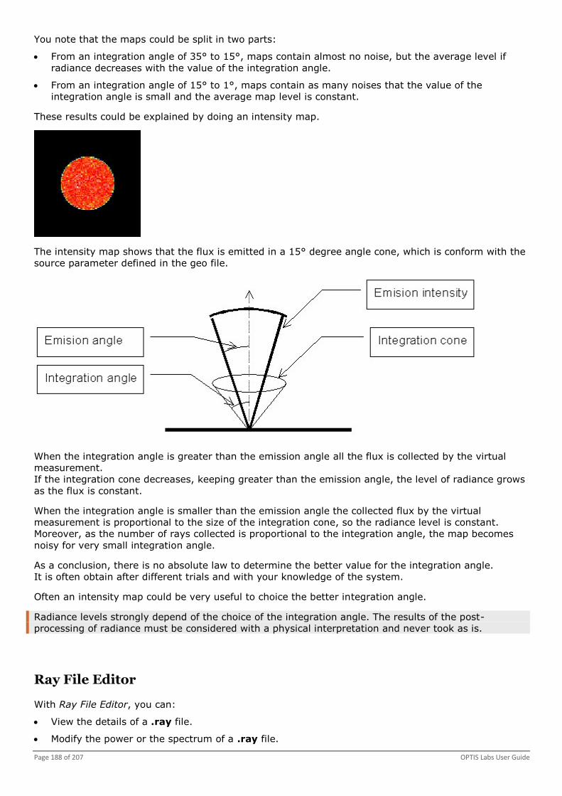
Page 188 of 207 OPTIS Labs User Guide
You note that the maps could be split in two parts:
From an integration angle of 35° to 15°, maps contain almost no noise, but the average level if
radiance decreases with the value of the integration angle.
From an integration angle of 15° to 1°, maps contain as many noises that the value of the
integration angle is small and the average map level is constant.
These results could be explained by doing an intensity map.
The intensity map shows that the flux is emitted in a 15° degree angle cone, which is conform with the
source parameter defined in the geo file.
When the integration angle is greater than the emission angle all the flux is collected by the virtual
measurement.
If the integration cone decreases, keeping greater than the emission angle, the level of radiance grows
as the flux is constant.
When the integration angle is smaller than the emission angle the collected flux by the virtual
measurement is proportional to the size of the integration cone, so the radiance level is constant.
Moreover, as the number of rays collected is proportional to the integration angle, the map becomes
noisy for very small integration angle.
As a conclusion, there is no absolute law to determine the better value for the integration angle.
It is often obtain after different trials and with your knowledge of the system.
Often an intensity map could be very useful to choice the better integration angle.
Radiance levels strongly depend of the choice of the integration angle. The results of the post-
processing of radiance must be considered with a physical interpretation and never took as is.
Ray File Editor
With Ray File Editor, you can:
View the details of a .ray file.
Modify the power or the spectrum of a .ray file.

Ray File Tools Page 189 of 207
Display the spectrum of a .ray file.
Repair an invalid .ray file.
Add two .ray files.
The relative power of ray and the new power of the resulting .ray file are automatically computed.
Mix all the ray in the .ray file.
Invert directions of ray.
Import or export (ASCII format).
Import Radiant and ASAP ASCII .ray file.
Import TechnoTeam source file (.erf files).
Import ASAP DIS ray file (.dis file).
Import a list of .ray files (.rayfileslist file).
To import a set of ray files in one step, you must create a .txt file listing the names of each file to
be imported.
Set the relative energy of each ray to 1.0.
Recompute the relative energy of each ray.
This divides all relative energy by the maximum.
Maximal Ray number value is 72 million rays.
Using the Ray File Editor
1. From Start menu, click All Programs, OPTIS, OPTIS Labs, Ray File Tools, Ray File Editor.
A window appears.
2. Click File, Open..., or to browse a .ray file.
You can import see page 189 or export see page 190 files.
You can use data downloaded from OSRAM Opto Semiconductors see page 190.
By clicking Edit, Repair or , you can repair a ray file.
3. Set the parameters see page 192.
You must save each .ray file.
You must take care not to overwrite .ray files as you might need the basic one for a different
binning and thus different emission.
4. Close the window.
Importing and Exporting
Importing a File
1. Click File, Import... or click .
2. Browse to select a file.
FILES EXTENSIONS
Text .txt
Rayset ASCII .asap, .out
Radiant ASCII .radiant
Technoteam Ray .erf
DIS Ray .dis

Page 190 of 207 OPTIS Labs User Guide
FILES EXTENSIONS
Ray Files List .raysfileslist
For more details about Radiant ASCII format, you can view Importing Radiant Imaging Files see
page 190.
3. Click Open.
A window appears.
4. Save the file as a .ray file.
5. Click Save.
Importing Radiant Imaging Files
Radiant imaging files have .rs7 or .rs8 extension.
From ProSource you must generate rays in the Lightools rayset format.
You must then export a ray file from ProSource compatible with SPEOS.
A ProSource licence is required to use ProSource or ProSource dlls.
1. Rename the Lightools .ray file as .radiant.
2. From the Ray File Editor, click File, Import... or click .
3. Browse to select a Radiant ASCII file.
RayEditor also imports the power of the Radiant Imaging source as it is included in the .radiant
file.
4. Click Open.
Exporting a File
1. Click File, Export... or click .
2. Type a file name.
3. Select a format.
FILES EXTENSIONS
Text .txt
DIS Ray Files .dis
4. Click Save.
The conversion is processing.
Using Data Downloaded from OSRAM Opto Semiconductors
1. Log on the OSRAM Website.
2. Download the library of OSRAM Ray Files.

Ray File Tools Page 191 of 207
In the downloaded Zip, you can find:
The orientation of the .ray file (PDF or JPEG),
The geometry of the optical system (STEP, IGES, SLDPRT) with the same global orientation as the
.ray files,
.ray files with different sizes (100k, 500k, 5M).
Content of the zip – Monochromatic source emission
For white LED, you find a blue and a yellow portion of the final .ray file.
To model correctly the LED emission, these two .ray files need to be prepared separately and then
put together.
Content of the zip – White source emission
3. Define the LED type if you are going to use sources with a narrow, monochromatic spectrum, or a
white light.
In case of using a source with a narrow spectrum, you can directly create a ray file source in the
OPTIS software.
You must use a support geometry as 1 point - 2 lines to create the Ray File Source in the software
respecting the orientation given for the .ray file (PDF or JPEG in the ZIP).
In SPEOS Standalone, you have to create a surface whose vectors I and J give the direction of the
ray file source.
In OptisWorks and SPEOS CAA V5 Based, only two lines are needed.
In case of using white light, it is first necessary to use the Ray File Editor and to prepare the
.ray file that will be used for the .ray file source.
For the white LED, you find two .ray files, one for the blue and one for the yellow emission.
Both have their corresponding spectrum and the typical flux already given.
To create the final .ray file it is necessary to adjust the power of both components.
4. From the Ray File Editor, open one of the yellow .ray files (100k, 500k, 5M).
If needed, you can adjust the power of the single .ray file, each for the blue and the yellow
portion, according to the designated emission (see therefore the PDF provided by OSRAM).

Page 192 of 207 OPTIS Labs User Guide
The default value for the power is the standard value given in the PDF of the zip folder. This value
must be adjusted according to the binning that will be used.
Both, blue and yellow part of the final .ray file have already the correct spectrum applied.
Parameters of Ray File Editor
Polarization data is as following:
I: ellipse big axis normalized vector (o, p, q) 3 float ( such as o*o+p*p+q*q=1 )
r: equal to J / I (small axis divided by big axis) 1 float ( 0 <= r <= 1 )
s: right or left polarization 1 float ( 0:right or 1:left )
I is orthogonal to the photon direction (l, m, n): l*o+m*p+n*q=0
J is orthogonal to I and to the photon's direction.
In the .ray files, (o, p, q, r, s) must be added to each ray.
nRs is the number of specular Reflections.
nRd is the number of diffuse Reflections.
nTs is the number of specular Transmissions.
nTd is the number of diffuse Transmissions.
In Power box, you can type the power value and click Update.
You must select the unit.
By clicking Edit, Change spectrum... or , you can select the spectrum type.
By selecting Blackbody, you can type the temperature value in Kelvins.
By selecting Monochromatic, you can type the value in nanometers.
By selecting Sampled, you must browse a Spectrum file.
You click to use the spectrum editor.
For more details, you can view Spectrum Editor see page 49.
By clicking , you can display the spectrum. You must adjust first the wavelength sampling by
typing the number of wavelengths value.

Ray File Tools Page 193 of 207
By clicking Edit, Add another ray file... or , you can add a new .ray file.
By clicking Edit, Invert direction of rays or , you can invert the directions of all rays.
By clicking Edit, Mix all rays in the file or , you can mix all the rays.
By clicking , you can change the relative value of each ray in the .ray file.
This is required when importing or creating .ray files. All containing rays have the same, very small
value as for example 1*10–6.
This function is similar to e/emax.
In case of having very small values for each ray and the values are not equally, you can click to
adjust the relative energy of each ray.
This is used to reach better performance for the calculation.
The ray with the highest energy becomes 1 and all the others are multiplied relatively to the first
ray.
The relative energy remains the same.

Page 194 of 207 OPTIS Labs User Guide
PREFERENCES
Monitor
The Monitor tab is available from Virtual Photometric Lab see page 100, Virtual Human Vision Lab see
page 69, User Material Editor see page 52, Spectrum Editor see page 49, Advanced Scattering Surface
Editor see page 16, BSDF - BRDF - Anisotropic Surfaces Viewer see page 17, Virtual Reality Lab see
page 121 and Real Time Lab.
With Monitor tab, you can indicate the characteristics of the monitor.
Monitor parameters are used to perform true color rendering especially in Virtual Photometric Lab.
You can improve the spectral maps' display and avoid the color disparity for a given spectral map
according to the monitor.
All parameters are set by default for an average CRT monitor. Details can be found here
(http://www.color.org/sRGB.html).
To obtain these values, you can ask your monitor's manufacturer or you can measure then with a
calibration tool or the spectrometer available for example with SPEOS Standalone.
Display
In Display box, you must select the display type.
When selecting SIM2 HDR display, you can display results on SIM2 HDR screens.
When selecting SIM2 HDR display, other parameters are not available.
When selecting SIM2 HDR display with Virtual Reality Lab, it is not possible to activate Human
Vision functions as Glare.
To avoid any display problems, SIM2 HDR monitor has to be dedicated for rendering and a
standard monitor for interface.
You must use the multiscreen mode to manage both monitors. For more details, you can view
Multiscreen see page 130.
You should not create any immersive view directly from the HDR screen .
When selecting SIM2 HDR display with Real Time Lab,
You must select Screen definition from Window, Full screen definition.
You must click Edit general preferences, enter 100% value for Rendering Definition for
Complete and Partial.
You must always have one pixel of the display window on only one pixel of the HDR screen.
Chromaticity Values
In Chromaticity values table, you can change the chromaticity values x and y of Red, Green, Blue
and White.
Gamma Correction
Details about Gamma correction can be found here (http://www.poynton.com/GammaFAQ.html).
In Correction Type group box, you must select the way to perform gamma correction.
By selecting Sampled Gamma, the gamma correction is performed by using the result of the
monitor calibration with the spectrometer.
By selecting Fitted Gamma, the gamma correction is performed by using the table underneath.
It is possible to define a different value of Gamma and Gain for each primary color but generally
the same value is satisfactory.
Gamma and Gain values can be obtained from your monitor's manufacturer.
Preferences Page 195 of 207
White Point Luminance
In White Point Luminance, you can type the white luminance level which gives the monitor's
dynamic.
White Point Luminance value has to be the maximum luminance of a white zone displayed by the
used screen.
By clicking , you can launch the monitor calibration to get parameters.
Colorimetry
The Colorimetry tab is available from Virtual Photometric Lab see page 100, User Material Editor see
page 52, Spectrum Editor see page 49, Advanced Scattering Surface Editor see page 16, BSDF - BRDF
- Anisotropic Surfaces Viewer see page 17 and Real Time Lab.
With Colorimetry tab, you can select the standard data used for colorimetric calculations.
You can also change the gamma parameter of your monitor to have a more realistic display.
Illuminant
In Illuminant box, you can select the reference illuminant.
Standard Observer Data
In Standard observer data box, you can select the CIE standard and the sampling.
Data are used from the color computation from the spectrum.
Color Standard Description
In Color standard description box, you can browse a .cls file to define the default colorimetric
standard to be displayed on the colorimetric diagram.
For more details about CLS file, you can view Parameters of Chromaticity Coordinates Tool see page
44.
Default Colorimetric System
In Default colorimetric system box, you can select the default colorimetric system to be used for
the colorimetric diagram.
Printing
The Printing tab is available from Virtual Photometric Lab see page 100, Spectrum Editor see page 49
and BSDF - BRDF - Anisotropic Surfaces Viewer see page 17.
With Printing tab, you can define information related to the print.
By selecting Default, you set values are the one that are in your computer, the user's name and
the company.
By selecting User defined, you can browse a .bmp file.
Spectrometer
The Spectrometer tab is available from Advanced Scattering Surface Editor see page 16, Spectrum
Editor see page 49 and User Material Editor see page 52.
You must have connected the OPTIS Software to the spectrometer.
With Spectrometer tab, you can insure the quality of the measurement by calibrating each
spectrometer with the four coefficients.

Page 196 of 207 OPTIS Labs User Guide
These coefficient values can be obtained on the calibration form supplied with the spectrometer.
Virtual Photometric Lab
The Virtual Photometric Lab tab is available from Virtual Photometric Lab see page 100.
This tab is only used for OptisWorks and SPEOS Standalone software.
You can set or save options and settings that would be used every time a XMP map is opened.
All XMP results take these options by default.
By selecting the Show rulers check box, you can display rulers.
You can click Ruler parameters....
By selecting the Show primary graduations or Show secondary graduations check box, you
can display primary or secondary graduations.
You can click Graduations parameters....
By selecting the Show primary grid or Show secondary grid check box, you can display primary
or secondary grid.
You can click Grid parameters....
By selecting the Show axis on cross check box, you can display axis on cross.
By selecting the Snap cross to grid check box, you can snap cross to grid.
By selecting the Show tool tip check box, you can display tool tip.
By selecting the Show gray around the map check box, you can display gray around the map.
By selecting the Fill shape check box, you can fill shape.
Directories
The Directories tab is available from the Virtual Photometric Lab see page 100, Virtual 3D Photometric
Lab see page 65, User Material Editor see page 52, Spectrum Editor see page 49, Advanced Scattering
Surface Editor see page 16 and BSDF - BRDF - Anisotropic Surfaces Viewer see page 17.
In Standard Windows directories group box, you can add standard shortcut for Open and Save
dialog boxes.
In User directories box, you can add your own shortcut for Open and Save dialog boxes.
In Exclude file type box, you can exclude some file types from OPTIS Software directory
management.
From the Help list, you can select the documentation language.
In case the language documentation does not still exist, default language is the english.
3D View
The Preferences window is available from the BSDF-BRDF-Anisotropic Surfaces Viewer see page 18,
Intensity Viewers see page 151 and the User Material Editor see page 58.
With Preferences, you can define parameters of the 3D display. This is useful to have a more precise
view to parameterize the meshing.

Preferences Page 197 of 207
In Radial Mesh Control group box, you can type the regular subdivisions and the adaptative
subdivisions values.
You can click Default Values to restore default values.
In Mesh reference group box, you must select Geosphere or Sphere theta/phi.
With high values, the loading time is bigger.
Within SPEOS Standalone software, the display is different.
By selecting the Antialiasing check box, you can have a better drawing of lines in 3D view by
avoiding notched lines.
By selecting the Phong check box, you can display 3D view without meshing.
Selecting the Phong check box can cause some problems with ellipsoid, which do not appear in
shading view, and with OSB files if normals have wrong orientation.
Without phong With phong
By selecting the Triangle check box, you can have a better way to mesh the object.
If some problems occur when displaying the 3D view, you must click to clear the check box.
By selecting the UV Axis & Normals check box, you can display UV axis of each face used for
texture on OSB faces.
Normals is used to define the orientation convention for BSDF.
In the 3D view, red and green axis of each faces represent the UV system and blue axis the
normal. The system can be direct or indirect.
The blue axis which is displayed gives the emission direction for the emissive surfaces and
indicates the convention for the 180° BSDF.
The direction related to the blue axis is used for the angles with incidence from 0 to 90° of the
BSDF.

Page 198 of 207 OPTIS Labs User Guide
If this direction does not fit, on the OSB it is possible to change the selected face orientation with
the Invert normal contextual menu which changes the OSB face topology.
By selecting the UV Isos 0.5 check box, you can display the Isos at U=V=0.5 which correspond to
the blue lines in the 3D view.
In the Number of first pattern to display (TXT texture) and Number of patterns to display
(TXT texture) boxes, you can type values which are used to display a TXT texture.
If the first value is N0 and the second one N, all the patterns in the text file between N0 and
N0+N-1 are displayed.
In the Number of repetitions to display (Brep texture) box, you can type a value which is
used to display a Brep texture.
When defining a system including a huge number of patterns, it is not possible to display all these
patterns in the 3D view.
Using the number of patterns or the number of repetitions, you can display a part of the texture in
order to check visually your texture definition.
Virtual 3D Photometric Lab
The Virtual 3D Photometric Lab tab is available from Virtual 3D Photometric Lab see page 65.
With Virtual 3D Photometric Lab tab, you can set and save display settings that are used every time a
new file is generated from a simulation.
Display
By selecting the Decorations check box, you can display the 3D view tool.
For more details, you can view Using 3D view tool.
By selecting the View Mesh check box, you can display the intensity envelope with wireframe.
By selecting the Mesh limit check box, you can display the mesh limit.
By selecting the Legend check box, you can display the legend.
By selecting the Axis check box, you can display the axis.
By selecting the Clip plane check box, you can display the clip plane.
By selecting the Contour check box, you can display the contour.
You can select the Colored check box to color contour.

Preferences Page 199 of 207
You can select the Annotation check box to display value of each contour line.
You can select a value in the both level lists.
Transparent
In Transparent box, you can move the slider to set the transparency.
Maximum Levels Number
In Maximum levels number box, you can define the maximum levels number to display results.
You can use more than 30 color levels.
Xm3 Filtering
By clicking Xm3 filtering..., you can set a standard filtering.
It only uses neighbors without any considerations regarding values of these neighbors.
In Pass number box, you must type the number of times the filtering algorithm is called.
0 value means there is no filtering.
Devices Preferences
The Devices Preferences tab is available from Virtual Reality Lab see page 121.
Computer's Devices
The Computer's Devices box is composed of:
Platform
GPU or CPU
Device (Microprocessor or graphic card)
Only one device can be selected unless the Virtual Reality Lab is launched a second time.
Real Time
The Real Time tab is available from Real Time Lab.
Wavelength Resampling
You can edit wavelengths.
Defaults
You can define default attributes of sources and geometries.
TFCalc
With TFCalc tab, you can set parameters that are used by TFCalc.

INDEX
3
3D Curve • 147, 148, 150, 152, 197
3D Energy Density Lab • 142
3D Map Post-Processing • 67
3D View • 18, 59, 153, 197
A
Absorption Variation • 56
Active Stereoscopy (Frame sequential mode) • 127
Adding Slaves to the Configuration • 140
Advanced Scattering Surface Editor • 16, 42, 195, 196, 197
Analyzing Colorimetric Data • 71, 77, 101, 113
Anisotropic BSDF Surface • 17, 19, 25
Anisotropic BSDF Surface Overview • 19
Anisotropic Scattering Surface • 25
Area • 136
Areas of Look At • 80, 81, 83, 89
Auto-calculate Value Option • 27, 49
Autofill • 17, 48
Avatar • 135
Axis System • 133
B
BRDF, BTDF, BSDF, Anisotropic Measurement Models • 7
BSDF - BRDF - Anisotropic Surface Viewer • 17, 195, 196, 197
BSDF180 Overview • 25
BSDF180 Surface • 17, 18, 25
Building BSDF180 Surface • 25
C
Calculation Parameters • 154
Change Reflection or Transmission Spectrum • 26
Changing Reflection or Transmission Spectrum • 26
Cluster • 139
Coated Surface • 17, 27, 42, 50
Coated Surface Curve • 27, 42
Color Rendering Index • 50, 51
Color Selection • 38, 39
Colorimetric Data • 44
Colorimetry • 45, 62, 196
Complete Scattering Surface (BRDF) • 17, 23
Configuring the Network Management • 137, 139
Configuring the Windows Firewall • 139
Coupling Efficiency Viewer • 154
Creating a Display • 134

Creating a Stereo OptisVR • 123, 127
Creating a System Display • 134
Creating a Window • 135
Creating an Area • 136
Creating an Avatar • 135
Creating an Immersive View • 123, 125, 129
Creating an Observer View • 123, 130
Curves • 151
D
Defining the zero reference • 135, 136
Devices Preferences • 123, 141, 200
Directories • 197
Display • 134
Displaying 3D Curve • 152
Displaying Isolux Curves • 151
Displaying Polar Curves • 152
Displaying Sollner Curves • 147, 148, 153
DOE and Thin Lens Surface Editor • 32
DOE and Thin Lens Surface Overview • 32
Doing 3D Map Post-Processing • 66, 67
Doing Analysis • 71, 88
Doing Color Management • 71, 78
Doing Time Adaptation • 71, 88
Dye Editor • 55, 60
E
Editing Coated Surface Curve • 42
Editing Lab/Gloss Surface Properties • 38, 47
Editing Material Color • 53, 61
Editing Scattering Surface Curve • 43
Editing Surface Properties • 15, 17, 18, 27, 38, 41, 44
Editing the Color Rendering Index Value • 51
Editing the Preferences • 15, 17, 18, 27, 38, 41, 48, 50, 53, 64, 66, 70, 71, 101, 120, 142, 146
Eulumdat Viewer • 147
Example of Polarizers • 9
Exporting • 71, 101, 104
Exporting a File • 190, 191
Exporting an Image • 71, 104
Exporting to Conoscopic Map • 18, 26
Extended Map Format • 105, 106
F
Fluorescent Surface Editor • 37, 42
G
Gaussian Propagation Viewer • 159
General • 53
Generating a Spectrum • 50, 52

Glare Effect • 87
Glare Effect Overview • 85, 87
Glass Map Viewer • 159
Grating Surface Editor • 36
H
HDRI File Format • 72, 102, 105, 108
Human Vision • 125
I
IESNA LM-63 Viewer • 148
Importing • 101, 102
Importing a BMP Mask • 101, 102
Importing a File • 190
Importing an Image • 71, 102
Importing and Exporting • 102, 190
Importing Radiant Imaging Files • 191
Index Variation • 55
Integration Angle • 186, 188
Intensity Distribution Post-processing • 185
Intensity Viewers • 147
Isolux Curves • 147, 148, 150, 151
J
Jones Matrix Examples • 29
L
Lab/Gloss Surface Definition • 47
LABS • 65
LCD Surface • 39, 42
Legibility (CIE 145
2002 standard) • 90
Legibility and Visibility Analysis • 90
Light Behavior Models • 6
Look At • 80
M
Making Surface and Section Analysis • 66, 68, 71, 96, 101, 113
Making Volume and Section Analysis • 142, 144
Managing the Display • 66, 67, 71, 75, 101, 111, 122, 142, 143
Managing the Filtering • 101, 120
Material Color • 61
Monitor • 70, 123, 141, 195
MultiScreen • 131, 139, 195
N
Network Management • 137
Night Vision Goggles • 95, 118

O
Optical Design Viewers • 154
Optical Polished Surface • 13
OPTICAL PROPERTY EDITORS • 6
OPTIS Intensity Viewer • 150
Others Options • 49
Overview • 6, 161
P
Parameters • 177
Parameters of 3D Curve • 152
Parameters of 3D Map Post-Processing • 67, 68
Parameters of a Coated Surface • 27
Parameters of a Display • 134
Parameters of a DOE and Thin Lens Surface • 35, 36
Parameters of a Fluorescent Surface • 37
Parameters of a Grating Surface • 36
Parameters of a LCD Surface • 40
Parameters of a Polarizer Surface • 28
Parameters of a Rendering Surface • 38
Parameters of a Retro Reflecting Surface • 31
Parameters of a Rough Mirror Surface • 41
Parameters of a Simple Scattering Surface • 15
Parameters of a Spectrum • 50
Parameters of a SystemDisplay • 134
Parameters of a User Material • 53
Parameters of a Window • 136
Parameters of an Aberration Coefficient Calculation • 168
Parameters of an Advanced Scattering Surface • 17, 38
Parameters of an Area • 137
Parameters of an Avatar • 135
Parameters of Arc Lamp • 183
Parameters of Auto-calculate Value Option • 49
Parameters of Autofill • 48
Parameters of Bitmap or RGBE Import • 102
Parameters of Black Body • 180
Parameters of Chromaticity Coordinates Tool • 44, 48, 50, 52, 62, 78, 91, 113, 196
Parameters of Coated Surface Curve • 42
Parameters of Coupling Efficiency Viewer • 154, 156
Parameters of Fluorescent Lamp • 183
Parameters of Gaussian Propagation Viewer • 159
Parameters of Glass Map Viewer • 160
Parameters of Human Vision • 126
Parameters of Incandescent Lamp • 182
Parameters of Isolux Curves • 151
Parameters of Lab/Gloss Surface Properties • 47
Parameters of Lambertian Source • 178, 179

Parameters of LED • 178
Parameters of Legibility and Visibility Tools • 90
Parameters of Material Color • 61
Parameters of Multimodal Laser Diode • 180
Parameters of Network Management • 137, 138
Parameters of Night Vision Goggles • 95, 118
Parameters of Optical Fiber • 177
Parameters of Paraxial Data Viewer • 166
Parameters of Photometric Calc • 65
Parameters of Polar Curves • 152
Parameters of Polarization Option • 50
Parameters of Position and Orientation • 177, 184
Parameters of Ray File Editor • 190, 193
Parameters of Scattering Surface • 17, 18, 43, 197
Parameters of Spectrum • 178, 179, 180, 182, 183, 184
Parameters of Spectrum Generation • 52, 53
Parameters of Spot Diagram Viewer • 173
Parameters of Surface and Section Analysis • 68, 96, 114
Parameters of Surface Properties • 44
Parameters of Technoteam PF File Import • 102, 104
Parameters of the Color Rendering Index • 45, 52, 62, 78, 113
Parameters of the Eulumdat Viewer • 147
Parameters of the IESNA LM-63 Viewer • 148
Parameters of the Intensity Distribution Post-processing • 185
Parameters of the Map Properties • 186
Parameters of the OPTIS Intensity Viewer • 150
Parameters of the Virtual Lighting Controller • 99, 100, 117, 145
Parameters of the Virtual Lighting Controller VRL • 124
Parameters of Transverse Ray Aberrations Viewer • 171, 172
Parameters of User Defined Source • 179, 181
Parameters of Vision Parameters • 82, 89, 90
Parameters of Volume and Section Analysis • 144
Parameters of XMP Export • 72, 75, 105
Parameters to Change Reflection or Transmission Spectrum • 26
Paraxial Data Viewer • 161
Particles • 57, 58, 59
Passive Stereoscopy • 128
Perfect Mirror Surface • 13
Photometric Calc • 65
Polar Curves • 147, 148, 150, 152
Polarization • 8, 27, 42, 50
Polarizer Surface Editor • 27
Polarizer Surface V1.0 • 28, 29
Polarizer Surface V2.0 • 28, 30
Post-Processing • 185
Preferences • 44, 48, 64, 70, 101, 120, 146
PREFERENCES • 195

Preferences of Scattering Surface Curve • 43, 44
Printing • 196
R
Ray File Editor • 189
RAY FILE TOOLS • 177
Reading Precision • 71, 77, 101, 112, 187
Real Aberrations Coefficients Viewer • 168
Real Aberrations Viewer • 171
Real Time • 200
Rendering Surface Editor • 38
Retro Reflecting Surface Editor • 31, 42
Rough Mirror Surface Editor • 41, 42
S
Saving Results • 131
Scattering Phase Function • 57, 58, 197
Scattering Properties • 56, 61
Scattering Surface Curve • 15, 17, 31, 37, 40, 41, 42
Setting the Cluster for the Master • 139, 140
Simple BSDF Surface • 17, 19
Simple Scattering Surface Editor • 15, 42
Source Generator • 177
Spectrometer • 196
Spectrum Editor • 37, 38, 44, 48, 50, 51, 52, 60, 61, 62, 78, 113, 193, 195, 196, 197
Spectrum Generation • 52
Specular Constant for Anisotropic BSDF • 22
Spot Diagram Viewer • 173
Starting the MultiScreen Mode • 140
Stereo OptisVR • 127
Structure of Anisotropic BSDF Files • 20
Surface and Section Analysis • 68, 96, 113
Surface Optical Property Editors • 6
Surfaces Overview • 6
Switching Between HDRI Picture and Immersive View • 131
Switching between Stereo and Normal Mode • 130
System VR Configuration • 132
System VR Configuration Overview • 132
SystemDisplay • 134
T
TFCalc • 49, 200
TFCalc Import • 27, 49
Tools • 44
TXT File Format • 102, 105
U
Unpolished Surface • 13, 17
User Material Editor • 53, 195, 196, 197

Using 3D Energy Density Lab • 142
Using Auto-calculate Value Option • 49
Using Autofill • 48
Using Coupling Efficiency Viewer • 154
Using Data Downloaded from OSRAM Opto Semiconductors • 190, 191
Using Filtering Tools • 121
Using Gaussian Propagation Viewer • 159
Using Glass Map Viewer • 159
Using Human Vision • 125
Using Legibility and Visibility Tools • 71, 90
Using Look At • 71, 80
Using Night Vision Goggles • 71, 95, 101, 118
Using Other Filterings • 121
Using Paraxial Data Viewer • 165
Using Photometric Calc • 65
Using Polarization Option • 50
Using Real Aberrations Coefficients Viewer • 168
Using Real Aberrations Viewer • 171
Using Spot Diagram Viewer • 173
Using Sun Glasses / Colored Filter • 71, 93
Using Sun Glasses or Colored Filter • 101, 118
Using the Advanced Scattering Surface Editor • 16
Using the BSDF - BRDF - Anisotropic Surface Viewer • 17
Using the Coated Surface Editor • 27
Using the DOE and Thin Lens Surface Editor • 35
Using the Eulumdat Viewer • 147
Using the Filtering • 131
Using the Fluorescent Surface Editor • 37
Using the Glare Effect • 71, 87
Using the Grating Surface Editor • 36
Using the IESNA LM-63 Viewer • 148
Using the Intensity Distribution Post-processing • 185
Using the LCD Surface Editor • 40
Using the Multiscreen Autostart • 141
Using the OPTIS Intensity Viewer • 150
Using the Polarizer Surface Editor • 28
Using the Ray File Editor • 190
Using the Rendering Surface Editor • 38
Using the Retro Reflecting Surface Editor • 31
Using the Rough Mirror Surface Editor • 41
Using the SIM2 HDR Monitor • 141
Using the Simple Scattering Surface Editor • 15
Using the Source Generator • 177
Using the Spectrum Editor • 50
Using the Stereo Immersive View Correction • 129
Using the User Material Editor • 53
Using the Virtual Lighting Controller • 71, 99, 101, 116, 122, 124, 142, 145

Using the Virtual Photometric Lab • 101
Using the Virtual Reality Peripheral Network Autostart • 142
Using the XMP Filtering • 120
Using the XMP Map Post- processing • 186
Using Virtual 3D Photometric Lab • 66
Using Virtual Human Vision Lab • 70
Using Virtual Reality Lab • 123
Using Virtual Reality Peripheral Network • 141
Using Vision Parameters • 71, 82, 88
V
View • 42
VIEWERS • 147
Virtual 3D Photometric Lab • 66, 197, 199
Virtual Human Vision Lab • 51, 70, 195
Virtual Lighting Controller • 99, 116, 124, 145
Virtual Photometric Lab • 51, 101, 147, 148, 150, 195, 196, 197
Virtual Reality Lab • 122, 195, 200
Virtual Reality Lab Icons • 122
Virtual Reality Lab Management • 131
Virtual Reality Peripheral Network • 141
Visibility • 92
Vision Parameters • 82
Volume and Section Analysis • 144
W
Window • 135
X
XMP Map Post- processing • 186