Option Profit and Loss Attribution and Pricing: A New ...
46
THE JOURNAL OF FINANCE • VOL. LXXV, NO. 4 • AUGUST 2020 Option Profit and Loss Attribution and Pricing: A New Framework PETER CARR and LIUREN WU ∗ ABSTRACT This paper develops a new top-down valuation framework that links the pricing of an option investment to its daily profit and loss attribution. The framework uses the Black-Merton-Scholes option pricing formula to attribute the short-term option in- vestment risk to variation in the underlying security price and the option’s implied volatility. Taking risk-neutral expectation and demanding no dynamic arbitrage re- sult in a pricing relation that links an option’s fair implied volatility level to the underlying volatility level with corrections for the implied volatility’s own expected direction of movement, its variance, and its covariance with the underlying security return. A foolish consistency is the hobgoblin of little minds. —Ralph Waldo Emerson DIFFERENT MODELING FRAMEWORKS SERVE DIFFERENT purposes. A major focus of the existing option pricing literature is to derive option values that are inter- nally consistent across all strikes and maturities. The literature specifies the full dynamics of the underlying security price, including the full dynamics of its instantaneous variance rate, and performs valuation of all options by taking risk-neutral expectations of their terminal payoffs. The full dynamics specifi- cation creates a single reference distribution of the relevant terminal random variable, which is then used to take the expectation. Under this approach, even if the assumed dynamics are wrong, the valuations on the option contracts re- main consistent with one another relative to this erroneous reference. ∗ Peter Carr is with New York University. Liuren Wu is in the Department of Economics and Finance, Baruch College. We would like to thank Stefan Nagel (the Editor), the associate editor, and two anonymous referees. We would also like to thank Yun Bai; David Gershon; Kris Jacobs; Danling Jiang; Aaron Kim; Chun Lin; Jason Roth; Angel Serrat; Stoyan Stoyanov; seminar participants at Baruch College, Credit Suisse, RMIT, Stony Brook University, City University of New York Graduate Center, and the 2017 6th IFSID Conference on Derivatives for comments. Liuren Wu gratefully acknowledges the support of a grant from the City University of New York PSC-CUNY Research Award Program. We have read The Journal of Finance’s disclosure policy and have no conflicts of interest to disclose. Correspondence: Liuren Wu, Department of Economics and Finance, Baruch College, One Bernard Baruch Way, Box B10-225, New York, NY 10010; email: [email protected]. DOI: 10.1111/jofi.12894 C 2020 the American Finance Association 2271
Transcript of Option Profit and Loss Attribution and Pricing: A New ...
THE JOURNAL OF FINANCE • VOL. LXXV, NO. 4 • AUGUST 2020
Option Profit and Loss Attribution and Pricing:A New Framework
PETER CARR and LIUREN WU∗
ABSTRACT
This paper develops a new top-down valuation framework that links the pricing ofan option investment to its daily profit and loss attribution. The framework uses theBlack-Merton-Scholes option pricing formula to attribute the short-term option in-vestment risk to variation in the underlying security price and the option’s impliedvolatility. Taking risk-neutral expectation and demanding no dynamic arbitrage re-sult in a pricing relation that links an option’s fair implied volatility level to theunderlying volatility level with corrections for the implied volatility’s own expecteddirection of movement, its variance, and its covariance with the underlying securityreturn.
A foolish consistency is the hobgoblin of little minds.—Ralph Waldo Emerson
DIFFERENT MODELING FRAMEWORKS SERVE DIFFERENT purposes. A major focusof the existing option pricing literature is to derive option values that are inter-nally consistent across all strikes and maturities. The literature specifies thefull dynamics of the underlying security price, including the full dynamics ofits instantaneous variance rate, and performs valuation of all options by takingrisk-neutral expectations of their terminal payoffs. The full dynamics specifi-cation creates a single reference distribution of the relevant terminal randomvariable, which is then used to take the expectation. Under this approach, evenif the assumed dynamics are wrong, the valuations on the option contracts re-main consistent with one another relative to this erroneous reference.
∗Peter Carr is with New York University. Liuren Wu is in the Department of Economics andFinance, Baruch College. We would like to thank Stefan Nagel (the Editor), the associate editor, andtwo anonymous referees. We would also like to thank Yun Bai; David Gershon; Kris Jacobs; DanlingJiang; Aaron Kim; Chun Lin; Jason Roth; Angel Serrat; Stoyan Stoyanov; seminar participantsat Baruch College, Credit Suisse, RMIT, Stony Brook University, City University of New YorkGraduate Center, and the 2017 6th IFSID Conference on Derivatives for comments. Liuren Wugratefully acknowledges the support of a grant from the City University of New York PSC-CUNYResearch Award Program. We have read The Journal of Finance’s disclosure policy and have noconflicts of interest to disclose.
Correspondence: Liuren Wu, Department of Economics and Finance, Baruch College, OneBernard Baruch Way, Box B10-225, New York, NY 10010; email: [email protected].
DOI: 10.1111/jofi.12894C© 2020 the American Finance Association
2271
2272 The Journal of Finance R©
It is good to be consistent, but it is not good to be wrong. Unfortunately,the assumed dynamics of the underlying security price and its instantaneousvolatility often deviate strongly from reality. For example, to price long-datedoptions, this approach needs to make projections on the underlying securityprice and its instantaneous volatility far into the future. The accuracy of long-dated projections is understandably low, and seemingly innocuous stationarityassumptions on the instantaneous volatility dynamics often generate muchlower price variation (Giglio and Kelly (2018)) and much flatter implied volatil-ity smiles (Carr and Wu (2003)) in long-term contracts than actually observedin the data.
In practice, as long as one does not hold the contracts to maturity, one does notnecessarily need to make long-run predictions to trade long-dated contracts—An investor can hold a very long-dated contract for a very short period oftime. In this case, the investor is less concerned about the terminal payoffthan about the factors that drive profit and loss over the short holding period.In fact, the standard recommended practice of marking financial securities tomarket makes it vitally important that investors understand the magnitudeand sources of daily value fluctuations, regardless of their intended holdingperiod. The process of attributing an investment’s profit and loss (P&L) ona given date to different risk exposures is commonly referred to as the P&Lattribution process.
In this paper, we develop a new valuation framework that links the pricingof a security at a given point in time to its P&L attribution without directlyreferring to the terminal payoffs of the investment. The P&L attribution re-quires the specification of a risk structure for computing the investment’s riskexposures and magnitudes. We take an investment in a European option as anexample and perform the P&L attribution on the option contract via the explicitBlack-Merton-Scholes (BMS) option pricing formula. Black and Scholes (1973)and Merton (1973) derive their option pricing formula by assuming constant-volatility geometric Brownian motion dynamics for the underlying securityprice. Their assumption does not match reality as return volatilities tend tovary strongly over time. Nevertheless, their pricing equation has been widelyused by practitioners as a simple and intuitive representation of the optionvalue in terms of its major risk sources, that is, variations in the underlyingsecurity price and its return volatility. In addition to the security price and con-tract terms (such as strike and maturity), the pricing equation takes a volatilityinput that can be used to match the observed option price. The volatility inputthat matches the observed option price is commonly referred to as the BMSoption implied volatility.
A Taylor series expansion of the BMS option pricing formula attributes theoption investment P&L to partial derivatives in time, the underlying securityprice, and the option’s implied volatility. When the underlying security priceand the option’s implied volatility move continuously over time, expanding tothe first order in time and second order in price and volatility is sufficientto bring the residual error to an order lower than the length of the shortinvestment horizon.
Option Profit and Loss Attribution and Pricing 2273
Taking the risk-neutral expectation over the P&L attribution via the BMSpricing formula and demanding no dynamic arbitrage result in a simple pricingequation that relates the option’s implied volatility level to the underlyinginstantaneous volatility as well as corrections due to the implied volatility’sexpected direction, variance, and covariance with the security return.
In contrast to the traditional option pricing approach, which links the valuesof all option contracts to a single reference dynamics specification, our newapproach links the current fair value of one option contract’s implied volatilityto current conditional moments of log changes in the security price and thegiven contract’s implied volatility. This subtle—but vital—shift in perspectiveis due to the use of the option’s own implied volatility rather than the underlyingsecurity’s instantaneous variance rate as a state variable. This new perspectiveallows one to completely localize the valuation of an option contract’s impliedvolatility level at a given point in time to the moment conditions on the variationof this particular implied volatility at that point in time.
For comparison, one can regard the traditional option pricing framework asa bottom-up valuation approach, with the key focus being specifying the ap-propriate basis that centralizes the valuation of all contracts. The key strengthof this centralized bottom-up approach is that cross-sectional consistency ismaintained through the use of one set of reference dynamics. By contrast, ournew framework is a decentralized top-down approach. By pricing an option con-tract based only on its own risk-neutral moment conditions, the theory does notimpose cross-sectional consistency across different option contracts. The newapproach is decidedly local in terms of the investment horizon it considers, andvery much decentralized in terms of the contract it values.
Under this new approach, to compare the valuation of two or more distinctoption contracts, one must first compare the risk exposures and magnitudesof these contracts. One can impose common factor structures on the momentconditions of different contracts to link the valuations of these contracts. Never-theless, their commonality, or lack thereof, is left as an empirical determinationor theoretical construction, but not a no-arbitrage condition. Therefore, whilethe traditional bottom-up approach is about the search for the omnipotent ba-sis reference, our new top-down approach is more about accurate forecasts ofthe moment conditions for the particular contract. The two approaches do notdirectly compete, but rather complement each other. Dynamics specificationsfrom the traditional approach can provide insights for formulating hypothe-ses on moment condition estimation, while empirically identified co-movementpatterns in the moment conditions can provide guidance for the specificationof reference dynamics.
To illustrate, we explore the cross-sectional pricing implications of the newframework under various commonality assumptions. First, we define the at-the-money option at a given maturity as the particular option whose log strike-forward ratio is equal to half of the option’s total implied variance, which is theBMS risk-neutral mean of the log security return to maturity. The fair valuationof this at-the-money option does not depend on the variance and covariance ofthe implied volatility change, but depends only on its risk-neutral drift and theinstantaneous variance level. By imposing a common risk-neutral drift on two
2274 The Journal of Finance R©
nearby at-the-money option contracts, we can extract the common risk-neutraldrift from the term structure slope defined by these two nearby contracts.Alternatively, by assuming a common one-factor mean-reverting structure onthe at-the-money implied variance, we can define an at-the-money implied vari-ance term structure function as an exponentially weighted average of the short-and long-dated implied variances, analogous to implications from traditionalstochastic volatility models (e.g., Heston (1993)).
At a fixed time to maturity, we take the at-the-money implied variance asthe reference point and perform a vega hedge of other contracts using theat-the-money option. We can then represent the implied volatility skew of anoption contract relative to the at-the-money implied volatility at this maturityas a function of the implied volatility’s variance and covariance with the se-curity return. Assuming that proportional movements have common varianceand covariance within a certain strike range, we can extract the common vari-ance and covariance from the implied volatility smile shape within this strikerange.
Another way to look at the traditional option pricing framework is fromthe perspective of spanning as articulated by Bakshi and Madan (2000), whoregard the characteristic function of the underlying security return as the ba-sis that spans most derivative securities. The dynamics specification dictatesthe pricing of Arrow and Debreu (1954) securities, which spans the payoff ofmost contingent claims. The payoff spanning perspective has a strong cross-sectional focus. It is because of this focus that pricing errors from traditionaloption pricing models are often regarded as the starting point for statisticalarbitrage trading (e.g., Duarte, Longstaff, and Yu (2007), Bali, Heidari, andWu (2009)). By contrast, our new pricing framework focuses more on the risk-return trade-off for a particular contract, in that the pricing of the contract ismade consistent with one’s view on that contract’s risk exposures and magni-tudes, rather than with the pricing of other contracts. Because of this differentperspective, our new approach can take outsourced expert forecasts on risksand risk premiums underlying a particular investment, convert them into risk-neutral moment conditions, and directly generate pricing implications withoutneeding to understand the source or rationale of these forecasts. Conversely, wecan infer moment conditions from market prices and examine the informationcontent of these moment conditions. In empirical analysis on S&P 500 indexoptions, we show that the risk-neutral drift extracted from the at-the-moneyimplied volatility term structure can be used to forecast future implied volatil-ity movements, and the variance and covariance extracted from the impliedvolatility smile can be combined with historical moment estimates to gener-ate better future realized variance and covariance forecasts. We also showthat these forecasts can be incorporated profitably into investment decisions inthe derivative contracts. In contrast to traditional statistical arbitrage tradingbased on the reversion assumption on pricing errors, the time series varianceand covariance forecasts allow us to identify investment opportunities withbetter risk-return trade-offs. Although investors can in principle make moneyfrom both approaches, our new framework provides a complementary perspec-tive that can potentially expand profitable investment opportunities.
Option Profit and Loss Attribution and Pricing 2275
As the BMS pricing formula has been widely adopted in the industry asa transformation tool, P&L attribution based on the BMS pricing equationis also common (Bergomi (2016)). There also exists a valuation method inthe industry based on options’ BMS vega, vanna, and volga. The method iscommonly referred to as the vanna-volga model (Castagna and Mercurio (2007),Wystup (2010)). The model starts by defining a reference volatility level andgenerating a reference value for the option based on the BMS model. The pricedifference of the target contract from the reference value is assumed to be linearin the price differences of three pillar options from their respective referencevalues. The three coefficients are determined by equating the vega, vanna, andvolga of the target option and the portfolio of the three pillar options, with allof the greeks evaluated at the reference volatility. The method has been usedto value both European options and exotic options based on observed priceson three appropriately chosen pillar options. It relies on the idea that the riskexposures of an option contract, defined via the BMS representation, can beapproximately spanned by the risk exposures of three appropriately chosenoption contracts. The vanna-volga model is similar to our approach in thatit relies on the BMS pricing representation in defining risk exposures, but itis different otherwise in terms of both implementation and perspective. OurBMS risk exposures on a contract are computed against the implied volatilityof that contract instead of a reference volatility, and our pricing result linksthe implied volatility level of an option contract to its own risk-neutral momentconditions, rather than linking the value of one option contract to the valuesof three other option contracts. Indeed, the spanning perspective of the vanna-volga model is much closer to the traditional option pricing approach than toour risk-return trade-off perspective.
The industry has also proposed several variations of the vanna-volga pricingapproach. For example, like us, Arslan et al. (2009) and Gershon (2018) calcu-late the BMS risk exposures of a contract using the implied volatility of thatcontract instead of a reference volatility. However, both of these papers adoptthe spanning perspective of the vanna-volga model and demand consistencywith the observed prices of three pillars.
Also related is the strand of the practitioner literature that attempts to di-rectly model the implied volatility dynamics for the pricing of exotic contracts.1
These attempts, often referred to as market models of implied volatility, takethe observed implied volatility as given while specifying the continuous mar-tingale component of the volatility surface. From these two inputs, they seekto derive the no-arbitrage restrictions on the risk-neutral drift of the impliedvolatility dynamics. The approach is analogous to the Heath, Jarrow, and Mor-ton’s (1992) model on forward interest rates and can in principle be used to pricederivatives written on the implied volatility surface. What prevents these at-tempts from achieving their objective is that knowledge about the shape of thecurrent implied volatility surface places constraints on the specification of the
1 See, for example, Avellaneda and Zhu (1998), Schonbucher (1999), Hafner (2004), Fengler(2005), and Daglish, Hull, and Suo (2007).
2276 The Journal of Finance R©
continuous martingale component for its future dynamics. In this paper, ratherthan ignoring these constraints, we fully exploit them in building a simple, di-rect linkage between the current level of the implied volatility and its first andsecond risk-neutral moment conditions.
In the academic literature, Israelov and Kelly (2017) recognize the limita-tions of standard option pricing models and propose directly predicting the dis-tribution of the option investment return empirically. Earlier empirical analysisof option investment returns includes Coval and Shumway (2001) and Jones(2006). Several recent studies link option returns to various firm characteris-tics: An et al. (2014) link future option implied volatility variation to past stockreturn performance, Boyer and Vorkink (2014) link ex post option returns to exante implied volatility skew, Byun and Kim (2016) link option returns to theunderlying stock’s lottery-like characteristics, and Hu and Jacobs (2017) linkoption returns and the underlying stock’s volatility level. Our research sharesthe same shift of focus from terminal payoffs to the behavior of short-term in-vestment returns. Our theory provides a foundation for how to analyze optioninvestment returns and how to link the predicted investment return behaviorto its pricing.
The remainder of this paper is organized as follows. Section I introduces thenotation and establishes the P&L attribution for an option contract based onthe BMS pricing formula. Section II takes the risk-neutral expectation of thereturn attribution and derives the no-arbitrage pricing implications. Section IIIexamines the cross-sectional pricing implications of the theory under differentlocal and global commonality assumptions. Section IV performs empirical anal-ysis on S&P 500 index options and explores different applications of the newtheory. Section V discusses the theory’s general implications, its limitations,and the risk representations. Section VI concludes.
I. P&L Attribution on Option Investments
We consider a market with a risk-free bond, a risky asset, and one vanillaEuropean option written on the risky asset. For simplicity, we assume zerointerest rates and zero carrying costs/benefits on the risky asset. In practicalimplementation, one can readily accommodate a deterministic term structureof financing rates by modeling the forward value of the underlying security anddefining moneyness of the option against the forward. The risky asset can beany type of tradable security, but for concreteness we refer to it as the stock. Inthe United States, exchange-traded options on individual stocks are Americanstyle. To apply our new theory to American options, a commonly used shortcutis to extract the BMS implied volatility from the price of an American optionbased on some tree/lattice method and use the implied volatility to compute aEuropean option value for the same maturity date and strike.2
2 See Carr and Wu (2010) for a detailed discussion on data preprocessing of individual stockoptions.
Option Profit and Loss Attribution and Pricing 2277
We assume frictionless and continuous trading in the risk-free bond, thestock, and the option contract written on the stock. We assume no-arbitragebetween the stock and the bond. As a result, there exists a risk-neutral proba-bility measure Q, equivalent to the statistical probability measure P, such thatthe stock price S is a martingale. We further assume that the option valuewe seek does not allow arbitrage against any portfolio of the stock and theriskless bond.
We start by considering a long position in a European call option. Holdingthe call to expiry generates a P&L dictated by the terminal payoff of the call.Classic option valuation starts with the terminal payoff function and takesthe expectation of the terminal payoff based on assumptions governing thedynamics of the underlying asset price. Our new pricing approach focuses onthe instantaneous investment P&L over the next instant. The short-term P&Lfluctuation of the option investment is driven mainly by the option’s exposuresto various risk sources and the variation in these risk sources. Accordingly,our analysis focuses more on defining risk exposures and quantifying riskmagnitudes than on describing terminal payoffs.
We attribute the short-term investment P&L on the option contract by mak-ing use of the explicit BMS pricing formula. The formula attributes the vari-ation in an option contract’s value to variation in the calendar time t, theunderlying security price St, and the option’s BMS implied volatility It. For-mally, let B(t, St, It; K, T ) denote the BMS representation of the option valueas a function of the three variates (t, St, It) for a European call option contractwith strike price K and expiry date T . The pricing formula is given by
B(t, St, It; K, T ) ≡ St N
(−k − 1
2 I2t τ
It√
τ
)− KN
(−k + 1
2 I2t τ
It√
τ
), (1)
where N(·) denotes the cumulative normal function, τ ≡ T − t the time tomaturity, and k ≡ ln(K/St) the relative strike. We henceforth use the termsz± ≡ (k ± 1
2 I2t τ ) to represent the convexity-adjusted moneyness of the call un-
der the risk-neutral measure and the share measure, respectively, in the BMSmodel environment.
For a given option contract, the BMS pricing formula represents the optionvalue at time t as a function of the stock price St and the option impliedvolatility It. As long as the option price does not allow arbitrage against theunderlying risky stock and the riskless bond, one can always find a positiveimplied volatility input to the BMS pricing formula to match that price (Hodges(1996)). The BMS pricing formula builds a monotonic linkage between theoption price and the option’s implied volatility, and captures all random shocksto the option (other than shocks to the underlying security price level) throughthe implied volatility.
Using the BMS pricing equation, we can attribute the instantaneous P&Lof the option investment to the variation in the calendar time, the stock price,
2278 The Journal of Finance R©
and the implied volatility,
dB = [Btdt + BSdSt + BIdIt
]+[
12
BSS(dSt)2 + 12
BII(dIt)2 + BIS(dStdIt)]
+ Jt,
(2)
where we suppress the arguments (t, St, It; K, T ) of the pricing function and useBt, BS, BI , BSS, BII , and BIS to denote the partial derivatives (sensitivities) ofthe pricing function against the calendar time t, the security price S, and theoption’s implied volatility I. The partial derivatives are commonly referred toas the option’s theta (Bt), delta (BS), vega (BI), gamma (BSS), volga (BII), andvanna (BIS), respectively. The first bracket collects first-order derivatives, thesecond bracket collects second-order derivatives, and the last term Jt capturesthe contribution of potential higher order derivatives due to random jumps inthe stock price and option implied volatility. When both the stock price andthe option implied volatility show purely continuous movements, the first andsecond derivatives capture all of the relevant movements for the option priceover a short time interval. We henceforth assume continuous dynamics andlink option pricing to its first- and second-order derivatives/exposures.
II. Risk-Neutral Expectation and Implied Volatility Valuation
We assume continuous dynamics, take the expectation of the option P&Lattribution in equation (2) under the risk-neutral measure Q, and divide theexpected P&L by the instantaneous investment horizon dt,
Et[dB]dt
= Bt + BI Itμt + 12
BSSS2t σ 2
t + 12
BII I2t ω2
t + BIS ItStγt, (3)
where Et[·] denotes the expectation operation under the risk-neutral measureconditional on time-t filtration and μt the annualized risk-neutral expectedrate of change in the BMS implied volatility of the option contract,
μt ≡ Et
[dIt
It
]/dt, (4)
and σ 2t , ω2
t , and γt the time-t conditional variance and covariance rate of thestock return and the implied volatility change,
σ 2t ≡ Et
[(dSt
St
)2]/dt, ω2
t ≡ Et
[(dIt
It
)2]/dt, γt ≡ Et
[(dSt
St,
dIt
It
)]/dt. (5)
Under the zero financing cost assumption, the risk-neutral expected stock re-turn is zero.
Option Profit and Loss Attribution and Pricing 2279
The zero financing cost assumption and no dynamic arbitrage dictate thatthe risk-neutral expected return on the option investment is also zero,
0 = Bt + BI Itμt + 12
BSSS2t σ 2
t + 12
BII I2t ω2
t + BIS ItStγt. (6)
We can regard equation (6) as a pricing relation. As long as the option pricesatisfies no dynamic arbitrage and generates a risk-neutral expected return ofzero, the option price must satisfy the constraints imposed by this equation.This pricing equation is not based on the full specification of the underlyingsecurity price dynamics, but rather on the first and second conditional momentsof the security price and the option’s implied volatility movements at time t.
The pricing relation in (6) highlights the short-term trade-offs among thedifferent sources of expected gains and losses from holding an option. By beinglong in an option, one loses time value as calendar time passes. The rate of lossis captured by the option’s theta, Bt. This theta loss is compensated by expectedgains from the security price variation, measured by the security’s return vari-ance σ 2
t , due to the option’s positive gamma exposure BSS. Variation in theoption’s implied volatility (ω2
t ) and in its covariation with the security return(γt) induce additional expected gains or losses due to the option’s volga (BII)and vanna (BIS) exposures, respectively. The option’s positive vega exposure(BI) can be another source of expected gain or loss depending on the expecteddirection (μt) of the implied volatility movement. The no-arbitrage conditiondictates that the option be priced such that at any point in time these differentsources of expected gains and losses balance out to produce a zero risk-neutralexpected excess return on the investment.
THEOREM 1: Under continuous price and implied volatility movements andzero financing costs, no dynamic arbitrage requires that an option be priced tobalance out the option’s theta loss against the expected gains and losses fromthe option’s vega, gamma, volga, and vanna exposures at any point in time,
−Bt = BI Itμt + 12
BSSS2t σ 2
t + 12
BII I2t ω2
t + BIS ItStγt. (7)
The gains and losses from these exposures are determined by the expected rateof the option’s implied volatility movement (μt), the security’s return varianceσ 2
t , the implied volatility’s variance ω2t , and the covariance between the security
return and the implied volatility γt, respectively.
Under this pricing relation, determining whether an option is fairly priced atany point in time amounts to determining whether the option’s exposures arebalanced out with the associated first- and second-moment forecasts at thattime. The pricing relation does not specify how to determine these forecasts orhow the forecasts vary over time. Thus, an interesting feature of the pricingrelation is that the risk forecasting process can be completely separated fromthe pricing process.
2280 The Journal of Finance R©
COROLLARY 1: Under continuous price movements and constant implied volatil-ity for an option contract with zero financing, the theta loss is compensated fullyby the gamma gain,
−Bt = 12
BSSS2t σ 2
t .
When the option’s implied volatility does not move over time, the only sourceof variation comes from the security price and hence the theta loss is balancedout completely by the gamma gain. This is the case under the BMS modelenvironment when the instantaneous return volatility σ is a constant.
A particularly nice feature of the BMS pricing equation is that the BMS theta(Bt), cash vega (BI It), cash vanna (BIS ItSt), and cash volga (BII I2
t ) can all berepresented in terms of the BMS cash gamma (BSSS2
t ),
Bt = −12
I2t BSSS2
t , BI It = I2t τ BSSS2
t ,
BIS ItSt = z+BSSS2t , BII I2
t = z+z−BSSS2t .
(8)
The Appendix provides the derivation. For an option contract with strictly posi-tive cash gamma, we can define the option investment return as the investmentP&L per unit of cash gamma so that we can factor out the cash gamma compo-nent from the pricing relation in (7) to obtain the following algebraic equation
I2t = [
2τμt I2t + σ 2
t
]+ [2γtz+ + ω2
t z+z−]. (9)
THEOREM 2: Assuming continuous price and implied volatility movements, andperforming instantaneous P&L attribution on a European option investmentbased on the BMS pricing equation, we arrive at a no-arbitrage pricing relationbetween the time-t fair value of the option’s implied volatility level and the time-trisk-neutral conditional mean and variance of the implied volatility percentagechange (μt and ω2
t ), the conditional variance of the underlying security return(σ 2
t ), and the conditional covariance between the two (γt).
Compared to traditional option pricing practice, equation (9) represents anextremely simple formulation of the option’s fair value. Traditional option pric-ing emphasizes cross-sectional consistency as its chief objective. To achievethis objective, one specifies the full risk-neutral dynamics on the underlyingsecurity and prices all options by taking expectations of their terminal payofffunctions based on the same dynamics assumption. These assumed dynamicson the underlying security serve as a single yardstick for all option contracts.The same yardstick guarantees that valuations of all options are consistentwith this yardstick and hence with one another.
By contrast, by starting with a localized P&L attribution of one option con-tract, equation (9) only guarantees that the time-t valuation of this contract isconsistent with the first and second risk-neutral conditional moments of theunderlying security price and this option’s implied volatility. It guarantees no
Option Profit and Loss Attribution and Pricing 2281
dynamic arbitrage between this option contract and the underlying securityand cash under the assumed moment conditions, but nothing more. Thus, in-stead of providing a yardstick for analyzing cross-sectional consistency acrossdifferent option contracts, the new approach provides a more direct, top-downlinkage between the fair implied volatility valuation of an option contract atany given point in time and its conditional moment conditions at that time.In this sense, while traditional option pricing focuses on cross-sectional con-sistency across contracts, the new pricing relation focuses on the risk-returntrade-off for one particular contract.
III. Commonality and Cross-Sectional Pricing
The pricing relation in (9) applies to one particular option contract, with noreference to any other option contracts. This relation allows one to comparethe valuation of an option contract to one’s projection of the first- and second-moment conditions of the underlying security price and the option’s impliedvolatility. To make valuation comparisons across different option contracts un-der this framework, one must first make comparisons on the first and secondconditional moments of the corresponding option implied volatilities.
Under the BMS model environment, the implied volatilities of all options un-derlying the same security are the same. In reality, option implied volatilitiesat different strikes and maturities can differ; nevertheless, they tend to movetogether. Furthermore, the implied volatility levels tend to be closer to eachother and their co-movements tend to be stronger as the strike and maturitydistances between the option contracts become smaller. As such, the impliedvolatility surface across strikes and maturities tends to possess a smooth shape.These basic observations can serve as a starting point in analyzing the com-monalities and differences in the implied volatility movements across strikesand maturities underlying a given security.
In this section, under our new pricing framework, we examine the cross-sectional pricing implications of different commonality assumptions. We ex-amine the validity of some of the commonality assumptions in Section IV.The analysis demonstrates how the new pricing framework generates cross-sectional implications based on explicit commonality assumptions on the un-derlying moment conditions.
A. The At-the-Money Implied Variance Term Structure
To separate the term structure effect from the moneyness effect, we define theat-the-money option as the option with z+ = k + 1
2 I2t τ = 0, which corresponds
to the strike price that equates the relative strike k to the risk-neutral expectedvalue of ln(ST /St) under the BMS model environment.
At z+ = 0, equation (8) shows that the option has both zero volga and zerovanna. Investing in such an option only exposes the investor to delta, vega, andgamma risk. The pricing equation in equation (9) also simplifies as the termsin the second bracket are reduced to zero. If we use a different notation, At, to
2282 The Journal of Finance R©
denote the at-the-money implied volatility at a certain time to maturity τ ,3 wecan write the pricing equation for the at-the-money implied volatility as
A2t = 2τμt A2
t + σ 2t . (10)
The at-the-money option with z+ = 0 is the only strike point at which the optionhas both zero volga and zero vanna. It is also the only strike point at whichthe implied volatility level depends only on the risk-neutral expected rate ofchange of the implied volatility, but not on its variance and covariance with thesecurity return. The separation allows us to analyze expected volatility changesand the term structure without interference from the second-order effects.
To extract the expected rate of change from the at-the-money impliedvolatility term structure, we propose to make the following local commonalityassumption.
ASSUMPTION (Local commonality on rates of change): The expected rates ofchange for at-the-money implied volatilities of nearby maturities are the same,
μt(τ1) .= μt(τ2), (11)
when |τ1 − τ2| is small.
With the local commonality assumption, we can extract the common expectedrate of change from the implied variance slope within this maturity range.
PROPOSITION 1: When the implied volatilities of at-the-money option contractswithin a maturity range [τ1, τ2] share the same risk-neutral expected rate ofchange μt at time t, this common rate can be extracted from the at-the-moneyimplied variance slope within this maturity range,
μt = A2t (τ2) − A2
t (τ1)2(A2
t (τ2)τ2 − A2t (τ1)τ1
) . (12)
Equation (12) can be readily derived by applying equation (10) twice at thetwo maturities τ1 and τ2 with the common expected rate of change μt.
The accuracy and validity of the extracted common rate of change dependson both the data quality of the implied volatility observations and the actualstability of the rate of change across the term structure. In representing thelocal commonality assumption, equation (11) uses the approximate equal sign“ .=” to highlight the approximate nature of the assumption. Similarly, the term“local” is not an exact phrasing, either. The extracted rate of change from (12)represents an approximate estimate of the true underlying rate of change,with the approximation error decreasing as the maturity distance decreasesand when the variation in the rate of change is smaller. In Section IV, we
3 Where possible confusion is not a concern, we drop the functional dependence of At on the timeto maturity to reduce notational clutter.
Option Profit and Loss Attribution and Pricing 2283
examine when the local commonality assumption holds reasonably well andwhen the assumption can break down.
B. The Implied Volatility Smile
To isolate the moneyness effect from the term structure effect, we considervega hedging with the at-the-money contract of the same expiry, assumingstrong implied volatility co-movements for options at the same expiry. In doingso, we take the at-the-money implied volatility level At as given, and representthe implied volatility levels of other option contracts at the same expiry asspreads (skews) relative to the at-the-money implied volatility level.
In particular, if we assume that the expected rate of change scales propor-tionally with the at-the-money contract according to
μt I2t = μA
t A2t , (13)
we can subtract (10) from (9) to highlight the implied volatility smile effectacross moneyness,
I2t − A2
t = 2γtz+ + ω2t z+z−. (14)
At each strike and accordingly each moneyness level z±, the variance andcovariance of the implied volatility change (ω2
t , γt) jointly determine the degreeto which the implied variance level at that strike I2
t deviates from the at-the-money implied variance level A2
t . Thus, the shape of the implied volatility smileat any point in time is driven by how much the implied volatility is expected tomove over the next instant and how it is expected to co-move with the securityprice. If one expects the implied volatility to move a lot in the next instant, onecannot expect the implied volatility smile to be flat.
As the variance and covariance (ω2t , γt) jointly determine the shape of the im-
plied volatility smile, we can reverse-engineer and extract the market-expectedvariance and covariance from the observed shape of the implied volatility smile.To do so, we make local commonality assumptions on the movements of the im-plied volatilities across moneyness.
ASSUMPTION (Local commonality on variance and covariance rates): The vari-ance and covariance rates of implied volatilities across a range of strikes at thesame maturity are the same,
ω2t (k) .= ω2
t , γ2t (k) .= γt, (15)
for all k within a certain strike range.
As near-the-money options are the most actively traded, it is of high practi-cal interest to extract the variance and covariance of the at-the-money impliedvolatility by assuming common variance and covariance for strikes within acertain range of the forward, or equivalently, for the convexity-adjusted mon-eyness measure z+ to be within a certain range around zero.
2284 The Journal of Finance R©
It is often observed that the implied volatility smile tends to have a smoothshape, and that the implied volatilities at nearby strikes tend to co-movestrongly, a stylized observation that we document in Section IV. The local com-monality assumption in (15) amounts to assuming that the implied volatilitiesat nearby strikes move by the same expected proportional magnitude.
PROPOSITION 2: With the local commonality assumption in (13) and (15), wecan estimate the locally common variance and covariance from a simple locallinear cross-sectional regression of the implied variance spread (I2
t − A2t ) on the
two convexity-adjusted moneyness measures [2z+, z+z−].
In Section IV, we estimate the variance and covariance of the at-the-moneyimplied volatility from a cross-sectional regression within a narrow range ofmoneyness around zero, and we examine their information content in predict-ing future variation in implied volatility.
IV. Empirical Analysis on S&P 500 Index Options
We perform empirical analysis on S&P 500 index (SPX) options. SPX optionsare actively traded on the Chicago Board of Options Exchange (CBOE). We ob-tain the history of closing option prices and implied volatilities on SPX options,as well as the underlying index level and interest rate series, from the datavendor OptionMetrics. The sample period is from January 4, 1996 to April 29,2016, which spans 5,111 business days. Over the sample period, the index levelstarted at around 617 and ended at around 2,065, with an annualized dailyreturn volatility estimate of 19.5%.
The new theory prices an option on the basis of the first and second risk-neutral moment conditions of the implied volatility changes of the particularcontract. As the data comprise quotes on exchange-traded option contracts,we can easily compute the implied volatility changes of an option contractfollowing its variation over consecutive days. To examine how the statisticalmoment conditions of the implied volatility changes vary across moneyness andtime to maturity, and how such variation is related to the pricing of the impliedvolatility term structure and the implied volatility smile, we construct floatingseries on the implied volatility changes at different moneyness and time-to-maturity grids via local smoothing interpolation. First, we provide evidence onlocal commonality in the co-movements among the floating implied volatilitychange series. Second, based on the local commonality observations, we extractthe locally common expected rate of change from the at-the-money impliedvolatility term structure of adjacent maturities. We examine the informationcontent of the extracted rate of change in predicting future implied volatilitychanges. Third, we construct variance and covariance estimates of the floatingimplied volatility time series and compare them with the locally common risk-neutral variance and covariance estimates extracted from the local impliedvariance smile around at-the-money. We then examine the extent to whichthe future realized variance and covariance estimates can be predicted bytheir corresponding historical time series estimates and the cross-sectionally
Option Profit and Loss Attribution and Pricing 2285
extracted risk-neutral estimates. We also construct a trading strategy basedon the difference between the future variance and covariance forecasts andthe risk-neutral moments currently priced in the local smile. We show thatthe trading strategy can capture large risk premiums with high informationratios, and that this strategy is distinct from traditional statistical arbitragestrategies.
A. Construct Floating Series of Implied Volatility Percentage Changes
The new theory relates the fair level of the implied volatility of an optioncontract to the first and second risk-neutral moments of the changes in theimplied volatility of that contract. As the data we have are quotes on fixedoption contracts, we can readily compute their implied volatility changes byfollowing the pricing of each contract over consecutive days. Nevertheless, toexamine how the moment conditions of these implied volatility changes varyacross moneyness and time to maturity, we need to construct floating timeseries on implied volatility changes at fixed moneyness and time-to-maturitygrids. The constructed floating series also allow us to better explore both theglobal factor structures and the local commonalities in the implied volatilitychanges across the moneyness and time-to-maturity grids.
Most prior empirical studies examine the behavior of floating implied volatil-ity time series at fixed time to maturity and fixed moneyness. Changes in suchfloating implied volatility time series can be quite different from the fixed-contract implied volatility changes that we construct. The difference can beparticularly large when the implied volatility surface has a steep term struc-ture and/or a strong implied volatility skew or smile. Even if the implied volatil-ity of each option contract were to remain the same, sliding along the termstructure (due to time running forward) and along the skew (due to spot pricemovement) would still lead to large changes in the floating implied volatil-ity series. Conversely, even if the implied volatility surface—as a function oftime to maturity and standardized moneyness—were to remain the same, theimplied volatility for a particular option contract with fixed expiry date andstrike price can change as its time to maturity and its relative moneyness varyover time.
From the observations on fixed option contracts, we construct floating timeseries on both the implied volatility levels and the fixed-contract implied volatil-ity changes via local smoothing interpolation. Specifically, at each date t, foreach option contract i available on that date, we retrieve its implied volatilityon both date t, Ii
t , and the next business date t + 1, Iit+1, and we compute the log
percentage implied volatility change, Rit+1 ≡ ln(Ii
t+1/Iit ), on this option contract.
We then smooth interpolate to generate both the time-t level and the changeat floating time to maturity and moneyness points.
We construct the floating time series at a grid of five time-to-maturity levelsand nine moneyness levels. The chosen time-to-maturity (τ ) grids are at onemonth (30 days), two months (60 days), three months (91 days), six months
2286 The Journal of Finance R©
(182 days), and 12 months (365 days). The maturity spacing choice is similarto common industry practice with finer grid points at shorter maturities whereoption trading activity is concentrated and where the term structure variesthe most.
At each maturity, the moneyness grids are constructed based on the stan-dardized moneyness measure x ≡ z+/It
√τ , which can be interpreted as the
number of standard deviations by which the log strike ln(K) exceeds the meanof the log terminal price ln(ST ) under the BMS model environment. We buildthe grids up to two standard deviations with a uniform interval of half a stan-dard deviation, x = 0,±0.5,±1,±1.5,±2.
We estimate both the implied volatility level It and the log implied volatilitychange Rt+1 of an option contract at each maturity-moneyness grid (τ, x) vialocal averaging with the following weighting schemes. First, at each strike,there can be two quotes, one from the call option and the other from the putoption. We put more weight on the out-of-the-money option contract, whichtends to be more actively traded and hence tends to have a more reliablequote. We use one minus the absolute value of the option’s forward delta asthe weight, and further truncate the weight to zero when the absolute deltais greater than 80%. The truncation sets the weights on deep in-the-moneyoptions to zero when the absolute delta is over 80%, where the quotes tend tobecome unreliable.
Second, we weigh each observation based on its distance to the target logtime to maturity (ln τ ) and its distance to the target moneyness level (x) basedon an independent bivariate Gaussian kernel with default bandwidth choices.Taking logarithm on time to maturity gives more resolution to the shorter timeto maturity.
Taken together, to construct the implied volatility level and percentagechange of an option contract at a target maturity-moneyness grid (τ, x), weweigh each contract i according to
wi = (1 − |δi|)I|δi |<.8 exp(
− (xi − x)2
2h2x
)exp
(− (ln τi − ln τ )2
2h2τ
), (16)
where δi denotes the BMS forward delta of the option and (hx, hτ ) denote thetwo bandwidths.
Our interpolation scheme is based on industry best practice. Common vari-ations in the interpolation scheme include the relative weighting between calland put options at the same strike and the degree of smoothing applied tothe quotes. Small variations in the interpolation methodology do not affect thegeneral conclusion of the analysis.
B. Local Commonality and Global Factor Structures
Our new theory links an option’s implied volatility level to its own first andsecond risk-neutral conditional moments. To extract the moment conditionsfrom the observed implied volatility level via reverse-engineering, we propose
Option Profit and Loss Attribution and Pricing 2287
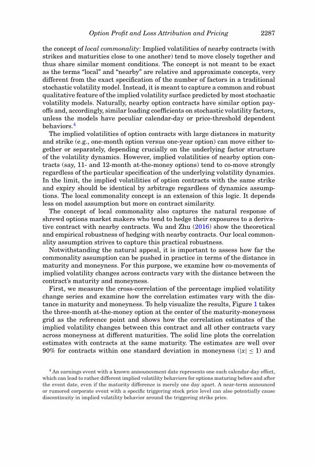
the concept of local commonality: Implied volatilities of nearby contracts (withstrikes and maturities close to one another) tend to move closely together andthus share similar moment conditions. The concept is not meant to be exactas the terms “local” and “nearby” are relative and approximate concepts, verydifferent from the exact specification of the number of factors in a traditionalstochastic volatility model. Instead, it is meant to capture a common and robustqualitative feature of the implied volatility surface predicted by most stochasticvolatility models. Naturally, nearby option contracts have similar option pay-offs and, accordingly, similar loading coefficients on stochastic volatility factors,unless the models have peculiar calendar-day or price-threshold dependentbehaviors.4
The implied volatilities of option contracts with large distances in maturityand strike (e.g., one-month option versus one-year option) can move either to-gether or separately, depending crucially on the underlying factor structureof the volatility dynamics. However, implied volatilities of nearby option con-tracts (say, 11- and 12-month at-the-money options) tend to co-move stronglyregardless of the particular specification of the underlying volatility dynamics.In the limit, the implied volatilities of option contracts with the same strikeand expiry should be identical by arbitrage regardless of dynamics assump-tions. The local commonality concept is an extension of this logic. It dependsless on model assumption but more on contract similarity.
The concept of local commonality also captures the natural response ofshrewd options market makers who tend to hedge their exposures to a deriva-tive contract with nearby contracts. Wu and Zhu (2016) show the theoreticaland empirical robustness of hedging with nearby contracts. Our local common-ality assumption strives to capture this practical robustness.
Notwithstanding the natural appeal, it is important to assess how far thecommonality assumption can be pushed in practice in terms of the distance inmaturity and moneyness. For this purpose, we examine how co-movements ofimplied volatility changes across contracts vary with the distance between thecontract’s maturity and moneyness.
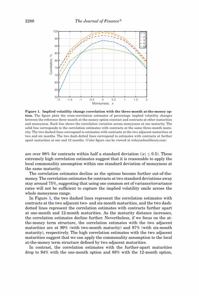
First, we measure the cross-correlation of the percentage implied volatilitychange series and examine how the correlation estimates vary with the dis-tance in maturity and moneyness. To help visualize the results, Figure 1 takesthe three-month at-the-money option at the center of the maturity-moneynessgrid as the reference point and shows how the correlation estimates of theimplied volatility changes between this contract and all other contracts varyacross moneyness at different maturities. The solid line plots the correlationestimates with contracts at the same maturity. The estimates are well over90% for contracts within one standard deviation in moneyness (|x| ≤ 1) and
4 An earnings event with a known announcement date represents one such calendar-day effect,which can lead to rather different implied volatility behaviors for options maturing before and afterthe event date, even if the maturity difference is merely one day apart. A near-term announcedor rumored corporate event with a specific triggering stock price level can also potentially causediscontinuity in implied volatility behavior around the triggering strike price.
2288 The Journal of Finance R©
-2 -1.5 -1 -0.5 0 0.5 1 1.5 2Moneyness, x
55
60
65
70
75
80
85
90
95
100
Cor
rela
tion,
%
123612
Figure 1. Implied volatility change correlation with the three-month at-the-money op-tion. The figure plots the cross-correlation estimates of percentage implied volatility changesbetween the reference three-month at-the-money option contract and contracts at other maturitiesand moneyness. Each line shows the correlation variation across moneyness at one maturity. Thesolid line corresponds to the correlation estimates with contracts at the same three-month matu-rity. The two dashed lines correspond to estimates with contracts at the two adjacent maturities attwo and six months. The two dash-dotted lines correspond to estimates with contracts at furtherapart maturities at one and 12 months. (Color figure can be viewed at wileyonlinelibrary.com)
are over 98% for contracts within half a standard deviation (|x| ≤ 0.5). Theseextremely high correlation estimates suggest that it is reasonable to apply thelocal commonality assumption within one standard deviation of moneyness atthe same maturity.
The correlation estimates decline as the options become further out-of-the-money. The correlation estimates for contracts at two standard deviations awaystay around 75%, suggesting that using one common set of variance/covariancerates will not be sufficient to capture the implied volatility smile across thewhole moneyness range.
In Figure 1, the two dashed lines represent the correlation estimates withcontracts at the two adjacent two- and six-month maturities, and the two dash-dotted lines represent the correlation estimates with contracts further apartat one-month and 12-month maturities. As the maturity distance increases,the correlation estimates decline further. Nevertheless, if we focus on the at-the-money term structure, the correlation estimates with the two adjacentmaturities are at 99% (with two-month maturity) and 97% (with six-monthmaturity), respectively. The high correlation estimates with the two adjacentmaturities suggest that we can apply the commonality assumption to the localat-the-money term structure defined by two adjacent maturities.
In contrast, the correlation estimates with the further-apart maturitiesdrop to 94% with the one-month option and 88% with the 12-month option,
Option Profit and Loss Attribution and Pricing 2289
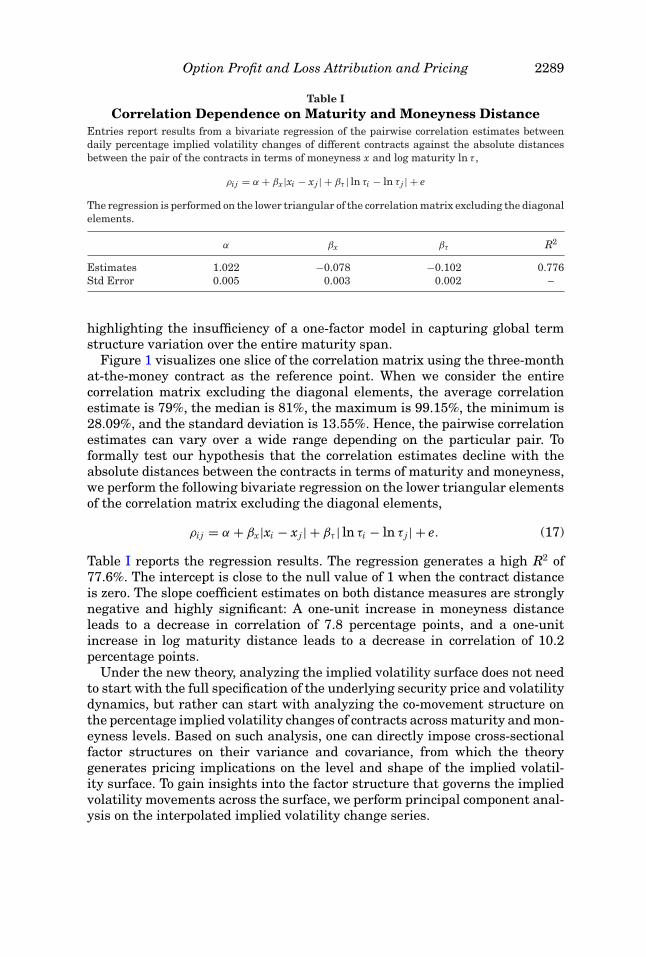
Table ICorrelation Dependence on Maturity and Moneyness Distance
Entries report results from a bivariate regression of the pairwise correlation estimates betweendaily percentage implied volatility changes of different contracts against the absolute distancesbetween the pair of the contracts in terms of moneyness x and log maturity ln τ ,
ρi j = α + βx |xi − xj | + βτ | ln τi − ln τ j | + e
The regression is performed on the lower triangular of the correlation matrix excluding the diagonalelements.
α βx βτ R2
Estimates 1.022 −0.078 −0.102 0.776Std Error 0.005 0.003 0.002 –
highlighting the insufficiency of a one-factor model in capturing global termstructure variation over the entire maturity span.
Figure 1 visualizes one slice of the correlation matrix using the three-monthat-the-money contract as the reference point. When we consider the entirecorrelation matrix excluding the diagonal elements, the average correlationestimate is 79%, the median is 81%, the maximum is 99.15%, the minimum is28.09%, and the standard deviation is 13.55%. Hence, the pairwise correlationestimates can vary over a wide range depending on the particular pair. Toformally test our hypothesis that the correlation estimates decline with theabsolute distances between the contracts in terms of maturity and moneyness,we perform the following bivariate regression on the lower triangular elementsof the correlation matrix excluding the diagonal elements,
ρi j = α + βx|xi − xj | + βτ | ln τi − ln τ j | + e. (17)
Table I reports the regression results. The regression generates a high R2 of77.6%. The intercept is close to the null value of 1 when the contract distanceis zero. The slope coefficient estimates on both distance measures are stronglynegative and highly significant: A one-unit increase in moneyness distanceleads to a decrease in correlation of 7.8 percentage points, and a one-unitincrease in log maturity distance leads to a decrease in correlation of 10.2percentage points.
Under the new theory, analyzing the implied volatility surface does not needto start with the full specification of the underlying security price and volatilitydynamics, but rather can start with analyzing the co-movement structure onthe percentage implied volatility changes of contracts across maturity and mon-eyness levels. Based on such analysis, one can directly impose cross-sectionalfactor structures on their variance and covariance, from which the theorygenerates pricing implications on the level and shape of the implied volatil-ity surface. To gain insights into the factor structure that governs the impliedvolatility movements across the surface, we perform principal component anal-ysis on the interpolated implied volatility change series.
2290 The Journal of Finance R©
Panel A. Explained Variation Panel B. Loading of the 1st PC
1 2 3 4 5 6 7 8 9 10Principle components
0
10
20
30
40
50
60
70
80
90
Exp
ain
ed v
ariatio
n, %
-2 -1.5 -1 -0.5 0 0.5 1 1.5 2Moneyness, x
0
0.05
0.1
0.15
0.2
0.25
0.3
0.35
1st
princi
ple
loadin
g
1 2 3 612
Panel C. Loading of the 2nd PC Panel D. Loading of the 3rd PC
-2 -1.5 -1 -0.5 0 0.5 1 1.5 2Moneyness, x
-0.4
-0.3
-0.2
-0.1
0
0.1
0.2
0.3
0.4
2nd p
rinci
ple
loadin
g
1 2 3 612
-2 -1.5 -1 -0.5 0 0.5 1 1.5 2Moneyness, x
-0.3
-0.2
-0.1
0
0.1
0.2
0.3
3rd
princi
ple
loadin
g 1 2 3 612
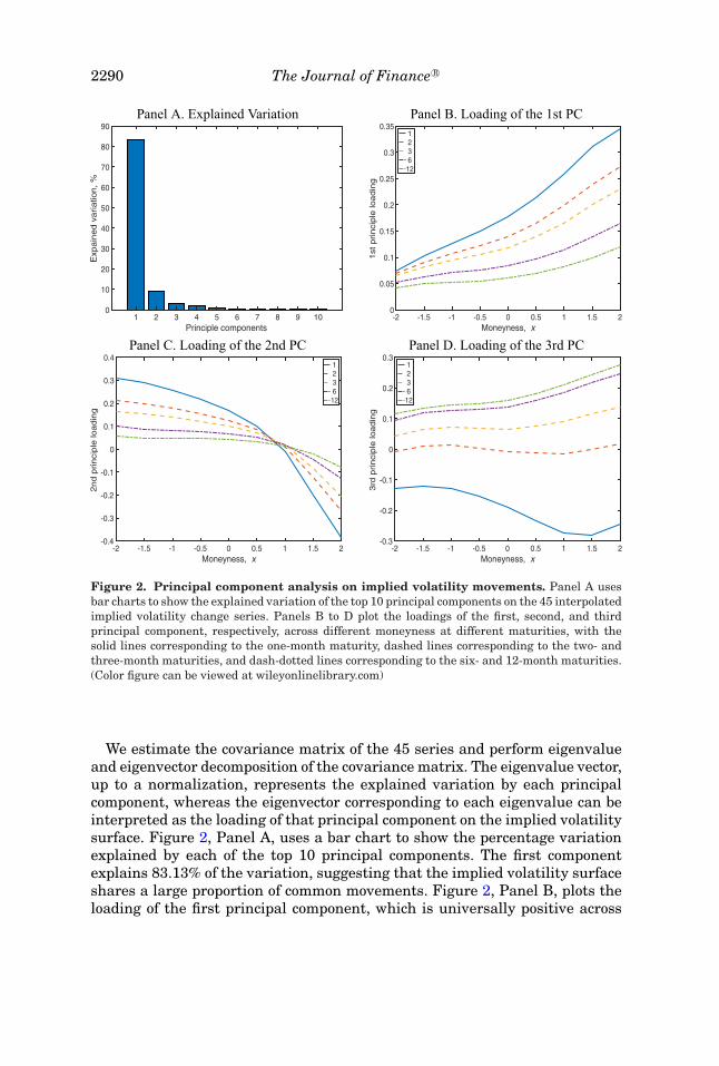
Figure 2. Principal component analysis on implied volatility movements. Panel A usesbar charts to show the explained variation of the top 10 principal components on the 45 interpolatedimplied volatility change series. Panels B to D plot the loadings of the first, second, and thirdprincipal component, respectively, across different moneyness at different maturities, with thesolid lines corresponding to the one-month maturity, dashed lines corresponding to the two- andthree-month maturities, and dash-dotted lines corresponding to the six- and 12-month maturities.(Color figure can be viewed at wileyonlinelibrary.com)
We estimate the covariance matrix of the 45 series and perform eigenvalueand eigenvector decomposition of the covariance matrix. The eigenvalue vector,up to a normalization, represents the explained variation by each principalcomponent, whereas the eigenvector corresponding to each eigenvalue can beinterpreted as the loading of that principal component on the implied volatilitysurface. Figure 2, Panel A, uses a bar chart to show the percentage variationexplained by each of the top 10 principal components. The first componentexplains 83.13% of the variation, suggesting that the implied volatility surfaceshares a large proportion of common movements. Figure 2, Panel B, plots theloading of the first principal component, which is universally positive across
Option Profit and Loss Attribution and Pricing 2291
all maturity and moneyness levels. The loading estimates are larger at shortermaturities and higher strikes, potentially highlighting their higher variation.
The second principal component explains 9.02% of the variation, which isstill highly significant albeit much smaller than the dominant first principalcomponent. Panel C of Figure 2 shows that the loading of this second principalcomponent has a distinct moneyness pattern as the loadings are positive atlow-strike regions and negative at high-strike regions, effectively capturingthe movement of the implied volatility skew at each maturity.
The third principal component explains 2.97% of the variation. Its effect,as shown in Panel D of Figure 2, is to capture the variation along the termstructure. At each moneyness, the loading is negative at short maturities butpositive at long maturities.
Taken together, within the confines of our data setting, the first three prin-cipal components explain over 95% of the variation on the implied volatilitysurface. The first principal component captures the movement of the overallimplied volatility level. The next two principal components capture the slopechanges of the surface along the moneyness and maturity dimensions.
The relative significance of the variations along the two slopes depends ondata sampling. The variation along the moneyness dimension tends to be moresignificant for exchange-traded options, which cover a wide range of moneynessbut a narrow range of maturity. For over-the-counter option quotes, which tendto span a narrower range of moneyness but a much wider range of maturity, theterm structure variation can become more significant. In general, it is impor-tant to realize that the principal component analysis is highly data dependent.To explain the same proportion of variation, one usually needs fewer principalcomponents if the data span a narrower strike or maturity range, but morewhen the data range is extended. This feature reveals the limitation of effortsto identify global factor structures. A seemingly sufficient factor structure un-der a certain data setting can often be easily rejected when the data rangeis expanded.
C. The At-the-Money Implied Variance Term Structure and Its Variation
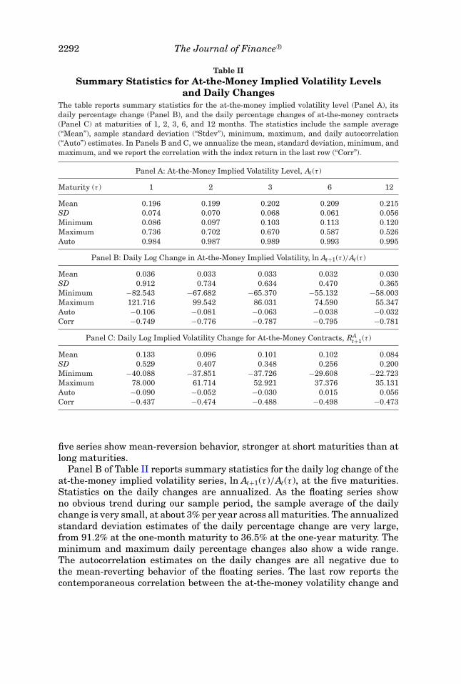
Table II, Panel A, reports summary statistics for the interpolated floating at-the-money implied volatility levels at the five maturities, At(τ ) ≡ It(τ, 0) at τ =1, 2, 3, 6, and 12 months. The sample average implied volatility level increasesas the time to maturity increases from one month to one year. The one-monthat-the-money implied volatility averages 19.6%, very close to the full-samplereturn standard deviation estimate of 19.5%. The sample average increaseswith maturity, reaching 21.5% at the one-year maturity.
The standard deviation of the at-the-money implied volatility series declineswith maturity from 7.4% at the one-month maturity to 5.6% at the one-year ma-turity. The range between the historical minimum and maximum also narrowswith increasing maturity, consistent with the decreasing standard deviation.The last row of the panel reports the autocorrelation of the floating series. All
2292 The Journal of Finance R©
Table IISummary Statistics for At-the-Money Implied Volatility Levels
and Daily ChangesThe table reports summary statistics for the at-the-money implied volatility level (Panel A), itsdaily percentage change (Panel B), and the daily percentage changes of at-the-money contracts(Panel C) at maturities of 1, 2, 3, 6, and 12 months. The statistics include the sample average(“Mean”), sample standard deviation (“Stdev”), minimum, maximum, and daily autocorrelation(“Auto”) estimates. In Panels B and C, we annualize the mean, standard deviation, minimum, andmaximum, and we report the correlation with the index return in the last row (“Corr”).
Panel A: At-the-Money Implied Volatility Level, At(τ )
Maturity (τ ) 1 2 3 6 12
Mean 0.196 0.199 0.202 0.209 0.215SD 0.074 0.070 0.068 0.061 0.056Minimum 0.086 0.097 0.103 0.113 0.120Maximum 0.736 0.702 0.670 0.587 0.526Auto 0.984 0.987 0.989 0.993 0.995
Panel B: Daily Log Change in At-the-Money Implied Volatility, ln At+1(τ )/At(τ )
Mean 0.036 0.033 0.033 0.032 0.030SD 0.912 0.734 0.634 0.470 0.365Minimum −82.543 −67.682 −65.370 −55.132 −58.003Maximum 121.716 99.542 86.031 74.590 55.347Auto −0.106 −0.081 −0.063 −0.038 −0.032Corr −0.749 −0.776 −0.787 −0.795 −0.781
Panel C: Daily Log Implied Volatility Change for At-the-Money Contracts, RAt+1(τ )
Mean 0.133 0.096 0.101 0.102 0.084SD 0.529 0.407 0.348 0.256 0.200Minimum −40.088 −37.851 −37.726 −29.608 −22.723Maximum 78.000 61.714 52.921 37.376 35.131Auto −0.090 −0.052 −0.030 0.015 0.056Corr −0.437 −0.474 −0.488 −0.498 −0.473
five series show mean-reversion behavior, stronger at short maturities than atlong maturities.
Panel B of Table II reports summary statistics for the daily log change of theat-the-money implied volatility series, ln At+1(τ )/At(τ ), at the five maturities.Statistics on the daily changes are annualized. As the floating series showno obvious trend during our sample period, the sample average of the dailychange is very small, at about 3% per year across all maturities. The annualizedstandard deviation estimates of the daily percentage change are very large,from 91.2% at the one-month maturity to 36.5% at the one-year maturity. Theminimum and maximum daily percentage changes also show a wide range.The autocorrelation estimates on the daily changes are all negative due tothe mean-reverting behavior of the floating series. The last row reports thecontemporaneous correlation between the at-the-money volatility change and
Option Profit and Loss Attribution and Pricing 2293
the security return. The estimates are strongly negative and of similar absolutemagnitudes across all maturities.
Panel C of Table II reports summary statistics for the daily log implied volatil-ity change of the at-the-money contracts, RA
t+1(τ ) ≡ Rt+1(τ, 0), which differ fromthe daily percentage changes of the floating series in Panel B. Compared toPanel B, the daily log changes on the fixed contracts show a higher annualizedsample mean, from 13.3% at the one-month maturity to 8.4% at the one-yearmaturity. According to the pricing equation in (12) and ignoring the variancerisk premium, the positive mean estimates imply an upward-sloping at-the-money implied variance term structure.
The annualized standard deviation estimates in Panel C are smaller thanthose on the changes of the floating series in Panel B. The estimates rangefrom 52.9% at the one-month maturity to 20% at the one-year maturity. Theminimum and maximum also form a narrower range than in Panel B.
The autocorrelation estimates on the implied volatility changes of at-the-money contracts are negative at short maturities, but become positive atlong maturities. Thus, mean-reversion in the floating series does not alwaystranslate into mean-reversion in the implied volatility changes of the fixedexpiry contracts.
The last row reports the contemporaneous correlation with the index return.The estimates are much smaller in absolute magnitude than the correlationestimates on the changes in the floating series. Overall, sliding along the termstructure and moneyness leads to large differences in the behavior of the float-ing and the fixed-contract implied volatility changes.
D. Extract Rate of Change from the At-the-Money Term Structure
Assuming that the proportional movements in implied volatilities are thesame for a pair of nearby at-the-money contracts, Proposition 1 allows us toextract the conditional risk-neutral drift of the implied volatility percentagechanges (μt) within this maturity range from the at-the-money implied vari-ance term structure slope defined by the two nearby contracts. The correlationestimates in Figure 1 show that the implied volatility movements of at-the-money contracts at adjacent maturities are extremely highly correlated, lend-ing support to the local commonality assumption for adjacent maturities. Wetherefore use the local at-the-money term structure slope defined by two ad-jacent maturities (τi, τi+1) to estimate the risk-neutral drift at the midpoint ofthe two maturities,
μt(τ i) = A2t (τi+1) − A2
t (τi)2(A2
t (τi+1)τi+1 − A2t (τi)τi)
, τ i = (τi + τi+1)/2. (18)
Specifically, we use the term structure slope defined by one-month and two-month at-the-money implied volatilities to estimate the drift at 1.5 months,the term structure defined by two-month and three-month at-the-moneyimplied volatilities to estimate the drift at 2.5 months, and so on. We then
2294 The Journal of Finance R©
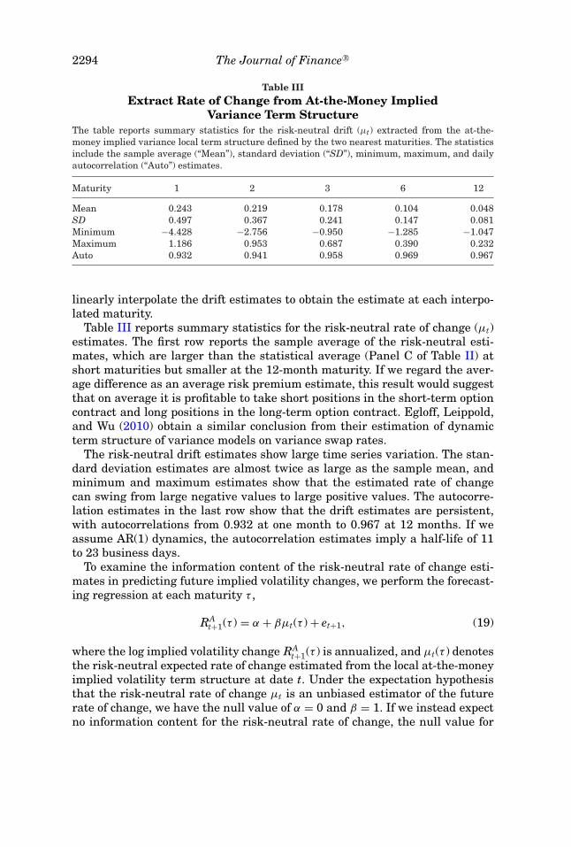
Table IIIExtract Rate of Change from At-the-Money Implied
Variance Term StructureThe table reports summary statistics for the risk-neutral drift (μt) extracted from the at-the-money implied variance local term structure defined by the two nearest maturities. The statisticsinclude the sample average (“Mean”), standard deviation (“SD”), minimum, maximum, and dailyautocorrelation (“Auto”) estimates.
Maturity 1 2 3 6 12
Mean 0.243 0.219 0.178 0.104 0.048SD 0.497 0.367 0.241 0.147 0.081Minimum −4.428 −2.756 −0.950 −1.285 −1.047Maximum 1.186 0.953 0.687 0.390 0.232Auto 0.932 0.941 0.958 0.969 0.967
linearly interpolate the drift estimates to obtain the estimate at each interpo-lated maturity.
Table III reports summary statistics for the risk-neutral rate of change (μt)estimates. The first row reports the sample average of the risk-neutral esti-mates, which are larger than the statistical average (Panel C of Table II) atshort maturities but smaller at the 12-month maturity. If we regard the aver-age difference as an average risk premium estimate, this result would suggestthat on average it is profitable to take short positions in the short-term optioncontract and long positions in the long-term option contract. Egloff, Leippold,and Wu (2010) obtain a similar conclusion from their estimation of dynamicterm structure of variance models on variance swap rates.
The risk-neutral drift estimates show large time series variation. The stan-dard deviation estimates are almost twice as large as the sample mean, andminimum and maximum estimates show that the estimated rate of changecan swing from large negative values to large positive values. The autocorre-lation estimates in the last row show that the drift estimates are persistent,with autocorrelations from 0.932 at one month to 0.967 at 12 months. If weassume AR(1) dynamics, the autocorrelation estimates imply a half-life of 11to 23 business days.
To examine the information content of the risk-neutral rate of change esti-mates in predicting future implied volatility changes, we perform the forecast-ing regression at each maturity τ ,
RAt+1(τ ) = α + βμt(τ ) + et+1, (19)
where the log implied volatility change RAt+1(τ ) is annualized, and μt(τ ) denotes
the risk-neutral expected rate of change estimated from the local at-the-moneyimplied volatility term structure at date t. Under the expectation hypothesisthat the risk-neutral rate of change μt is an unbiased estimator of the futurerate of change, we have the null value of α = 0 and β = 1. If we instead expectno information content for the risk-neutral rate of change, the null value for
Option Profit and Loss Attribution and Pricing 2295
Table IVPredict Implied Volatility Changes With the Term Structure Slope
The table reports the coefficient estimates, the absolute Newey-West’s t-values (in parentheses),and the R2s of the following forecasting regression at each maturity τ ,
RAt+1(τ ) = α + βμt(τ ) + et+1,
where the daily log implied volatility change of the at-the-money contract RAt+1(τ ) is annualized
and the risk-neutral expected rate of change μt(τ ) is extracted from the local at-the-money impliedvariance term structure defined by the two adjacent maturities. The t-values are computed with alag of one month. For the β estimates, the table reports the t-values for both the null hypothesis ofβ = 0 and the null hypothesis of β = 1.
Maturity α H : α = 0 β H : β = 0 H : β = 1 R2, %
1 −0.095 (0.59) 0.935 (2.56) (0.18) 0.312 −0.128 (1.01) 1.027 (3.06) (0.08) 0.343 −0.136 (1.15) 1.332 (3.26) (0.81) 0.346 −0.014 (0.16) 1.115 (2.20) (0.23) 0.16
12 0.072 (0.99) 0.243 (0.28) (0.88) 0.00
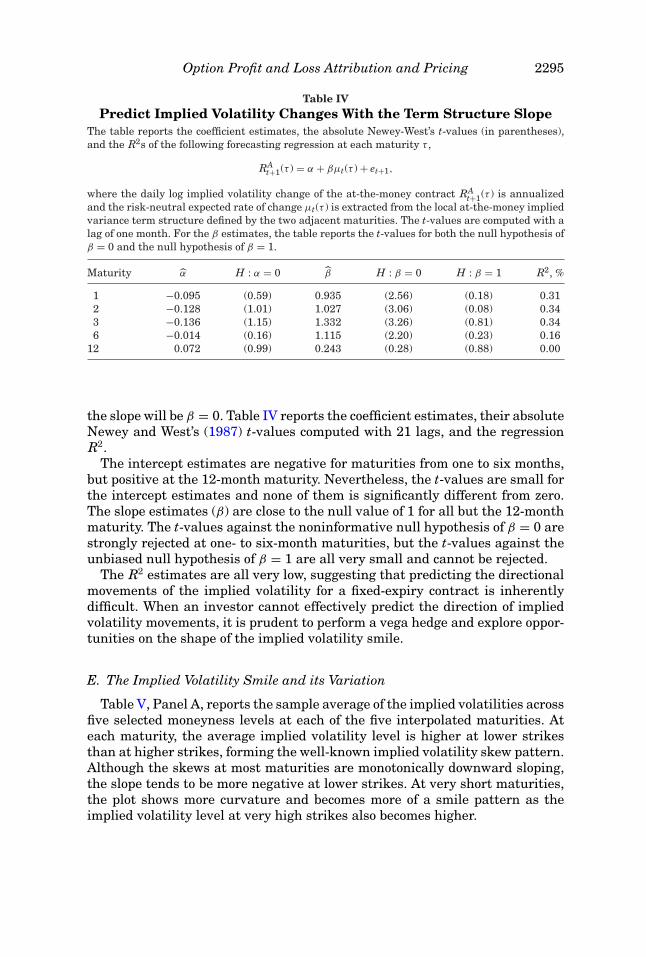
the slope will be β = 0. Table IV reports the coefficient estimates, their absoluteNewey and West’s (1987) t-values computed with 21 lags, and the regressionR2.
The intercept estimates are negative for maturities from one to six months,but positive at the 12-month maturity. Nevertheless, the t-values are small forthe intercept estimates and none of them is significantly different from zero.The slope estimates (β) are close to the null value of 1 for all but the 12-monthmaturity. The t-values against the noninformative null hypothesis of β = 0 arestrongly rejected at one- to six-month maturities, but the t-values against theunbiased null hypothesis of β = 1 are all very small and cannot be rejected.
The R2 estimates are all very low, suggesting that predicting the directionalmovements of the implied volatility for a fixed-expiry contract is inherentlydifficult. When an investor cannot effectively predict the direction of impliedvolatility movements, it is prudent to perform a vega hedge and explore oppor-tunities on the shape of the implied volatility smile.
E. The Implied Volatility Smile and its Variation
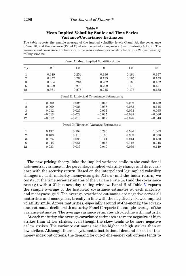
Table V, Panel A, reports the sample average of the implied volatilities acrossfive selected moneyness levels at each of the five interpolated maturities. Ateach maturity, the average implied volatility level is higher at lower strikesthan at higher strikes, forming the well-known implied volatility skew pattern.Although the skews at most maturities are monotonically downward sloping,the slope tends to be more negative at lower strikes. At very short maturities,the plot shows more curvature and becomes more of a smile pattern as theimplied volatility level at very high strikes also becomes higher.
2296 The Journal of Finance R©
Table VMean Implied Volatility Smile and Time Series
Variance/Covariance EstimatesThe table reports the sample average of the implied volatility levels (Panel A), the covariance(Panel B), and the variance (Panel C) at each selected moneyness (x) and maturity (τ ) grid. Thevariance and covariance are historical time series estimators constructed with a 21-business-dayrolling window.
Panel A: Mean Implied Volatility Smile
τ\x −2.0 1.0 0 1.0 2.0
1 0.349 0.254 0.196 0.164 0.1572 0.352 0.260 0.199 0.165 0.1533 0.354 0.264 0.202 0.166 0.1526 0.359 0.273 0.209 0.170 0.151
12 0.361 0.278 0.215 0.173 0.152
Panel B: Historical Covariance Estimates γt
1 −0.000 −0.025 −0.045 −0.082 −0.1522 −0.009 −0.026 −0.038 −0.063 −0.1153 −0.012 −0.025 −0.033 −0.053 −0.0956 −0.013 −0.022 −0.025 −0.038 −0.066
12 −0.012 −0.018 −0.019 −0.028 −0.048
Panel C: Historical Variance Estimates ωt
1 0.192 0.194 0.280 0.536 1.0632 0.103 0.118 0.166 0.303 0.6303 0.074 0.088 0.121 0.214 0.4506 0.045 0.051 0.066 0.112 0.248
12 0.033 0.033 0.040 0.069 0.149
The new pricing theory links the implied variance smile to the conditionalrisk-neutral variance of the percentage implied volatility change and its covari-ance with the security return. Based on the interpolated log implied volatilitychanges at each maturity moneyness grid Rt(τ, x) and the index return, weconstruct the time series estimates of the variance rate (ωt) and the covariancerate (γt) with a 21-business-day rolling window. Panel B of Table V reportsthe sample average of the historical covariance estimates at each maturityand moneyness grid. The average covariance estimates are negative across allmaturities and moneyness, broadly in line with the negatively skewed impliedvolatility smile. Across maturities, especially around at-the-money, the covari-ance estimates decline with maturity. Panel C reports the sample average of thevariance estimates. The average variance estimates also decline with maturity.
At each maturity, the average covariance estimates are more negative at highstrikes than at low strikes, even though the skew tends to be more negativeat low strikes. The variance estimates are also higher at high strikes than atlow strikes. Although there is systematic institutional demand for out-of-the-money index put options, the demand for out-of-the-money call options tends to
Option Profit and Loss Attribution and Pricing 2297
be more retail-driven and less systematic, leading to more idiosyncratic move-ments for out-of-the-money calls. These larger idiosyncratic movements mayhelp explain the larger absolute magnitude of the variance and covariance es-timates at higher strikes. On the other hand, the larger systematic demandfor out-of-the-money index put options may have pushed the implied volatilityskew steeper at lower strikes, despite the smaller absolute magnitudes of thevariance and covariance estimates. This disparity between demand and histor-ical magnitude of variation may present profitable opportunities for investorswho can manage the risk appropriately.
F. Extract Variance and Covariance Rates from the Implied Volatility Smile
Figure 1 shows that within one standard deviation of at-the-money (|x| ≤ 1),log implied volatility changes between the at-the-money contract and othercontracts are highly correlated, with correlation estimates over 90%. Based onthis evidence, we apply the local commonality assumption within one stan-dard deviation of the at-the-money option (|x| ≤ 1) and we extract the commonrisk-neutral variance and covariance rates by performing the cross-sectionalregression
I2t − A2
t = γt(2z+) + ω2t (z+z−) + et. (20)
At each date and maturity, we regress the implied variance difference fromthe at-the-money level against the moneyness measures 2z+ and z+z−. We con-strain the regression to the five moneyness levels within one standard deviationof at-the-money. We can readily convert the moneyness measure x to z+ andz− given the implied volatility estimate at each point. We impose zero inter-cept and constrain the regression coefficient ω2
t to be positive. The regressioncaptures the implied variance smile around at-the-money. A negative impliedvolatility skew will generate a negative covariance estimate γt, whereas a pos-itive curvature for the smile leads to a positive variance estimate ω2
t .Table VI reports summary statistics for the slope coefficients and the R2 es-
timates. Panel A shows that the covariance estimates are universally negativeacross all maturities and calendar days, suggesting that the implied volatilitysmiles on the S&P 500 index are persistently negatively skewed. The esti-mates show high time series persistence. The daily autocorrelation estimatesare high, from 0.978 at the one-month maturity to 0.995 at the 12-monthmaturity.
By choosing options around at-the-money in running the regression, we canregard the regression estimates as reflecting the moment conditions of theat-the-money contract. Comparing the average cross-sectional (CS) regressioncovariance estimates with the average historical time series (TS) estimates forthe at-the-money option in Table V, we find that on average the cross-sectionalestimates are more negative than the time series estimates, suggesting thatthe implied volatility skew tends to be steeper than warranted by the historicalbehavior of the covariation between the implied volatility and the index return.
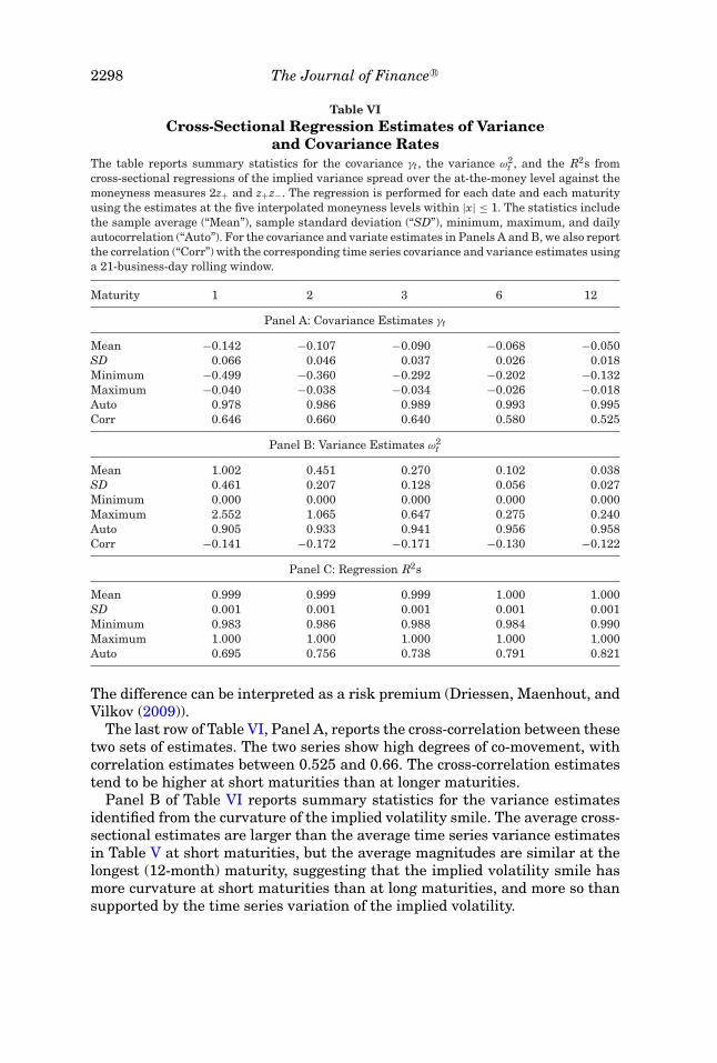
2298 The Journal of Finance R©
Table VICross-Sectional Regression Estimates of Variance
and Covariance RatesThe table reports summary statistics for the covariance γt, the variance ω2
t , and the R2s fromcross-sectional regressions of the implied variance spread over the at-the-money level against themoneyness measures 2z+ and z+z−. The regression is performed for each date and each maturityusing the estimates at the five interpolated moneyness levels within |x| ≤ 1. The statistics includethe sample average (“Mean”), sample standard deviation (“SD”), minimum, maximum, and dailyautocorrelation (“Auto”). For the covariance and variate estimates in Panels A and B, we also reportthe correlation (“Corr”) with the corresponding time series covariance and variance estimates usinga 21-business-day rolling window.
Maturity 1 2 3 6 12
Panel A: Covariance Estimates γt
Mean −0.142 −0.107 −0.090 −0.068 −0.050SD 0.066 0.046 0.037 0.026 0.018Minimum −0.499 −0.360 −0.292 −0.202 −0.132Maximum −0.040 −0.038 −0.034 −0.026 −0.018Auto 0.978 0.986 0.989 0.993 0.995Corr 0.646 0.660 0.640 0.580 0.525
Panel B: Variance Estimates ω2t
Mean 1.002 0.451 0.270 0.102 0.038SD 0.461 0.207 0.128 0.056 0.027Minimum 0.000 0.000 0.000 0.000 0.000Maximum 2.552 1.065 0.647 0.275 0.240Auto 0.905 0.933 0.941 0.956 0.958Corr −0.141 −0.172 −0.171 −0.130 −0.122
Panel C: Regression R2s
Mean 0.999 0.999 0.999 1.000 1.000SD 0.001 0.001 0.001 0.001 0.001Minimum 0.983 0.986 0.988 0.984 0.990Maximum 1.000 1.000 1.000 1.000 1.000Auto 0.695 0.756 0.738 0.791 0.821
The difference can be interpreted as a risk premium (Driessen, Maenhout, andVilkov (2009)).
The last row of Table VI, Panel A, reports the cross-correlation between thesetwo sets of estimates. The two series show high degrees of co-movement, withcorrelation estimates between 0.525 and 0.66. The cross-correlation estimatestend to be higher at short maturities than at longer maturities.
Panel B of Table VI reports summary statistics for the variance estimatesidentified from the curvature of the implied volatility smile. The average cross-sectional estimates are larger than the average time series variance estimatesin Table V at short maturities, but the average magnitudes are similar at thelongest (12-month) maturity, suggesting that the implied volatility smile hasmore curvature at short maturities than at long maturities, and more so thansupported by the time series variation of the implied volatility.
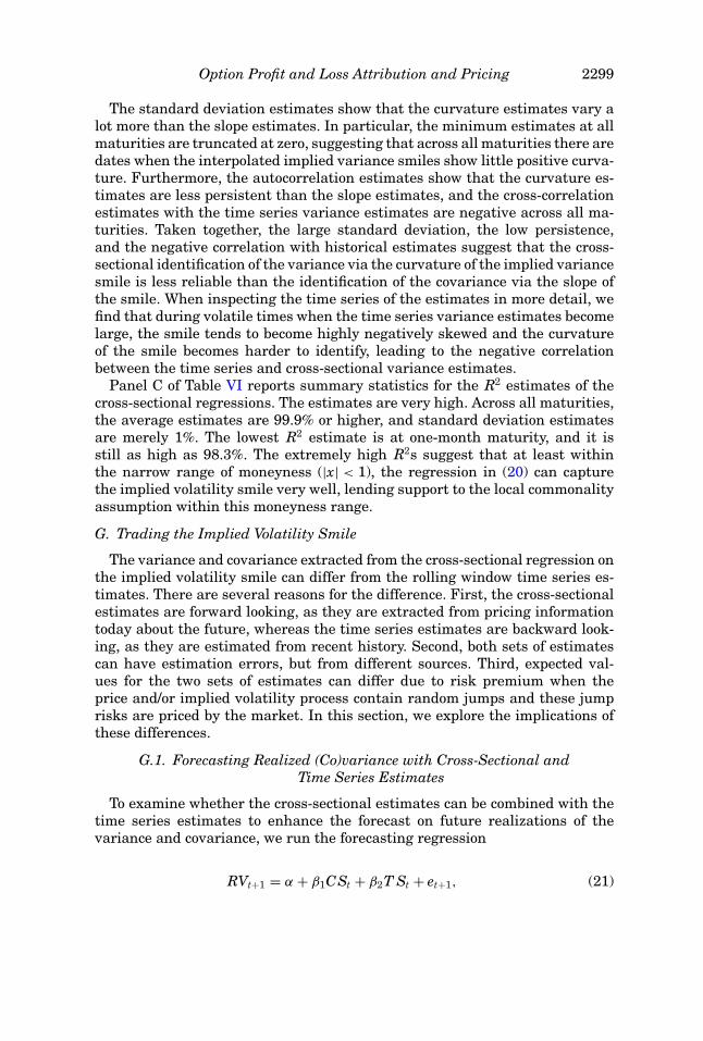
Option Profit and Loss Attribution and Pricing 2299
The standard deviation estimates show that the curvature estimates vary alot more than the slope estimates. In particular, the minimum estimates at allmaturities are truncated at zero, suggesting that across all maturities there aredates when the interpolated implied variance smiles show little positive curva-ture. Furthermore, the autocorrelation estimates show that the curvature es-timates are less persistent than the slope estimates, and the cross-correlationestimates with the time series variance estimates are negative across all ma-turities. Taken together, the large standard deviation, the low persistence,and the negative correlation with historical estimates suggest that the cross-sectional identification of the variance via the curvature of the implied variancesmile is less reliable than the identification of the covariance via the slope ofthe smile. When inspecting the time series of the estimates in more detail, wefind that during volatile times when the time series variance estimates becomelarge, the smile tends to become highly negatively skewed and the curvatureof the smile becomes harder to identify, leading to the negative correlationbetween the time series and cross-sectional variance estimates.
Panel C of Table VI reports summary statistics for the R2 estimates of thecross-sectional regressions. The estimates are very high. Across all maturities,the average estimates are 99.9% or higher, and standard deviation estimatesare merely 1%. The lowest R2 estimate is at one-month maturity, and it isstill as high as 98.3%. The extremely high R2s suggest that at least withinthe narrow range of moneyness (|x| < 1), the regression in (20) can capturethe implied volatility smile very well, lending support to the local commonalityassumption within this moneyness range.
G. Trading the Implied Volatility Smile
The variance and covariance extracted from the cross-sectional regression onthe implied volatility smile can differ from the rolling window time series es-timates. There are several reasons for the difference. First, the cross-sectionalestimates are forward looking, as they are extracted from pricing informationtoday about the future, whereas the time series estimates are backward look-ing, as they are estimated from recent history. Second, both sets of estimatescan have estimation errors, but from different sources. Third, expected val-ues for the two sets of estimates can differ due to risk premium when theprice and/or implied volatility process contain random jumps and these jumprisks are priced by the market. In this section, we explore the implications ofthese differences.
G.1. Forecasting Realized (Co)variance with Cross-Sectional andTime Series Estimates
To examine whether the cross-sectional estimates can be combined with thetime series estimates to enhance the forecast on future realizations of thevariance and covariance, we run the forecasting regression
RVt+1 = α + β1CSt + β2T St + et+1, (21)
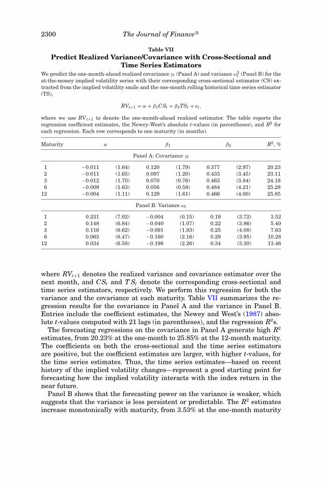
2300 The Journal of Finance R©
Table VIIPredict Realized Variance/Covariance with Cross-Sectional and
Time Series EstimatorsWe predict the one-month-ahead realized covariance γt (Panel A) and variance ω2
t (Panel B) for theat-the-money implied volatility series with their corresponding cross-sectional estimator (CS) ex-tracted from the implied volatility smile and the one-month rolling historical time series estimator(TS),
RVt+1 = α + β1CSt + β2TSt + et,
where we use RVt+1 to denote the one-month-ahead realized estimator. The table reports theregression coefficient estimates, the Newey-West’s absolute t-values (in parentheses), and R2 foreach regression. Each row corresponds to one maturity (in months).
Maturity α β1 β2 R2, %
Panel A: Covariance γt
1 −0.011 (1.64) 0.120 (1.79) 0.377 (2.97) 20.232 −0.011 (1.65) 0.097 (1.20) 0.433 (3.45) 23.113 −0.012 (1.70) 0.070 (0.76) 0.463 (3.84) 24.186 −0.009 (1.63) 0.056 (0.58) 0.484 (4.21) 25.28
12 −0.004 (1.11) 0.129 (1.61) 0.466 (4.00) 25.85
Panel B: Variance ωt
1 0.231 (7.02) −0.004 (0.15) 0.19 (3.72) 3.522 0.148 (6.84) −0.040 (1.07) 0.22 (3.86) 5.403 0.116 (6.62) −0.091 (1.83) 0.25 (4.08) 7.636 0.063 (6.47) −0.160 (2.16) 0.29 (3.95) 10.28
12 0.034 (6.58) −0.198 (2.26) 0.34 (3.30) 13.46
where RVt+1 denotes the realized variance and covariance estimator over thenext month, and CSt and T St denote the corresponding cross-sectional andtime series estimators, respectively. We perform this regression for both thevariance and the covariance at each maturity. Table VII summarizes the re-gression results for the covariance in Panel A and the variance in Panel B.Entries include the coefficient estimates, the Newey and West’s (1987) abso-lute t-values computed with 21 lags (in parentheses), and the regression R2s.
The forecasting regressions on the covariance in Panel A generate high R2
estimates, from 20.23% at the one-month to 25.85% at the 12-month maturity.The coefficients on both the cross-sectional and the time series estimatorsare positive, but the coefficient estimates are larger, with higher t-values, forthe time series estimates. Thus, the time series estimates—based on recenthistory of the implied volatility changes—represent a good starting point forforecasting how the implied volatility interacts with the index return in thenear future.
Panel B shows that the forecasting power on the variance is weaker, whichsuggests that the variance is less persistent or predictable. The R2 estimatesincrease monotonically with maturity, from 3.53% at the one-month maturity
Option Profit and Loss Attribution and Pricing 2301
to 13.45% at the 12-month maturity. The coefficient estimates on the historicaltime series estimator are all positive and statistically significant. The contribu-tion from the cross-sectional estimator is smaller and the coefficient estimatesbecome negative in all cases.
G.2. Risk-Return Trade-Off Trading based on Time Series Forecasts
Given a set of forecasts on future realized variance and covariance and as-suming common movements within a moneyness range, our theory generatesa breakeven value on the implied volatility smile. The breakeven value repre-sents the valuation of the implied volatility smile based on statistical forecastson the variance and covariance while assuming zero risk premium. When theobserved implied volatility smile differs from this valuation, the difference canbe viewed as a potential source of risk premium and a potentially profitabletrading opportunity. We examine the profitability using an out-of-sample in-vestment exercise.
Starting on January 3, 2000, at each date and for each option maturity, weuse a four-year rolling window to estimate the forecasting relation in (21) togenerate out-of-sample forecasts on the covariance γt and the variance ωt. Withthese forecasts, we construct the breakeven implied variance spread at the fourmoneyness levels x = ±0.5,±1.0,
I2t − A2
t = 2γtz+ + ω2t z+z−, (22)
where we take the observed at-the-money implied volatility At as given andgenerate fair valuations on the spreads. The two moneyness measures z+ andz− also depend on the implied volatility level. We construct the measures usingthe observed implied volatility level.
At each moneyness, we form vega-neutral spread option portfolios with theat-the-money contract and track the delta-hedged P&L over the next month.As out-of-the-money options tend to be more actively traded than in-the-moneyoptions, we form put spreads at low strikes and call spreads at high strikes.For each spread, we normalize the weight on the at-the-money contract to oneand take short positions in the out-of-the-money contract to make the spreadvega neutral.
We set the weight on each spread based on the difference between the ob-served implied variance spread I2
t − A2t from the market and the breakeven
valuation I2t − A2
t from equation (22),
wt =(
I2t − I2
t
)/A2
t , (23)
where the at-the-money implied variance is cancelled out in the numeratorand we divide the difference by the at-the-money implied variance level toobtain a proportional number. When the market-observed spread is higherthan the fair value, we long 100 × wt dollars of notional of the at-the-moneycontract and short the contract at the corresponding moneyness to make it
2302 The Journal of Finance R©
vega neutral. We hold the spread for 21 days while performing daily deltahedge with the underlying index futures. In option investments, because ofthe small value of the option contract relative to the potentially large riskexposures, investors often measure investments in terms of notional exposuresrather than the money spent or received from buying or selling the option.Investing 100 × wt notional dollars is equivalent to normalizing the index levelto $100 and investing wt shares in the normalized contract.
Table VIII reports summary statistics for the investment weights. Each panelreports one summary statistic. Within each panel, each column represents onemoneyness level x, and each row represents one time to maturity τ , representedin months. The average weights on the put spreads at x = −0.5 and −1 arepositive and on the call spreads at x = 0.5 and 1 are negative. The strategyis, on average, short out-of-the-money puts and long out-of-the-money calls,benefiting from the observation that on average the negative implied volatilityskews are steeper than warranted by the historical covariance estimates. Theaverage weights are larger in absolute magnitude for further out-of-the-moneyspreads at |x| = 1 than at |x| = 0.5, as are the standard deviation estimates.
Nevertheless, the minimum weights are negative and the maximum weightsare positive on all spreads, suggesting that the investments based on the timeseries forecasts can switch signs despite the average bias. Finally, the dailyautocorrelation estimates in Panel E show that the investment weights arehighly persistent. This high persistence suggests low turnover for the strategy.
In the three panels in Table IX, we track the delta-hedged P&L of each spreadportfolio and report its annualized mean, annualized standard deviation, andannualized information ratio. Table IX is similar to Table VIII in that withineach panel, each column represents one moneyness level and each row repre-sents one time to maturity. In addition to the four moneyness levels at eachmaturity, we add a column labelled “All,” which reports the P&L for investingin all four spreads at each maturity.
The sample averages of the P&L on all spread investments are positive.The investments show larger risk (standard deviation) at shorter maturitiesthan at longer maturities, and also at further out-of-money at |x| = 1 than at|x| = 0.5. The average P&L also varies with maturity and moneyness, but notas much as the risk. The net result is that the information ratios are higherfor investments at longer maturities than at shorter maturities. For example,combining the four spreads at the one-month maturity generates an annualizedinformation ratio of 0.52. The information ratio becomes increasingly larger asthe option maturity increases, reaching as high as 3.81 for investing in thefour spreads at the 12-month maturity. Several factors contribute to the lowprofitability of the trades on short-term contracts. First, short-term optionsare more sensitive to price and implied volatility jumps, a component absentfrom our pricing relation. Second, the forecasting results in Table VII showthat the R2 of the forecasting regression is lower at short maturities. Thus,our forecasts of the breakeven spreads are also less accurate, further reducingtrading performance. By contrast, for long-dated contracts, the variance andcovariance of the implied volatility series dominate the P&L variation of the
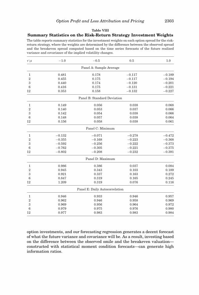
Option Profit and Loss Attribution and Pricing 2303
Table VIIISummary Statistics on the Risk-Return Strategy Investment WeightsThe table reports summary statistics for the investment weights on each option spread for the risk-return strategy, where the weights are determined by the difference between the observed spreadand the breakeven spread computed based on the time series forecasts of the future realizedvariance and covariance of the implied volatility changes.
τ\x −1.0 −0.5 0.5 1.0
Panel A: Sample Average
1 0.481 0.178 −0.117 −0.1892 0.455 0.175 −0.117 −0.1943 0.440 0.174 −0.120 −0.2016 0.416 0.175 −0.131 −0.221
12 0.353 0.158 −0.132 −0.227
Panel B: Standard Deviation
1 0.149 0.056 0.038 0.0682 0.140 0.053 0.037 0.0663 0.142 0.054 0.038 0.0666 0.148 0.057 0.038 0.064
12 0.156 0.058 0.038 0.061
Panel C: Minimum
1 −0.132 −0.071 −0.278 −0.4722 −0.355 −0.168 −0.223 −0.3683 −0.592 −0.256 −0.222 −0.3736 −0.762 −0.305 −0.221 −0.375
12 −0.802 −0.208 −0.232 −0.391
Panel D: Maximum
1 0.986 0.386 0.037 0.0842 0.945 0.343 0.103 0.1893 0.921 0.337 0.163 0.2726 0.847 0.319 0.165 0.245
12 1.209 0.319 0.076 0.116
Panel E: Daily Autocorrelation
1 0.946 0.933 0.946 0.9572 0.962 0.946 0.958 0.9693 0.969 0.956 0.964 0.9726 0.979 0.975 0.976 0.980
12 0.977 0.983 0.983 0.984
option investments, and our forecasting regression generates a decent forecastof what the future variance and covariance will be. As a result, investing basedon the difference between the observed smile and the breakeven valuation—constructed with statistical moment condition forecasts—can generate highinformation ratios.
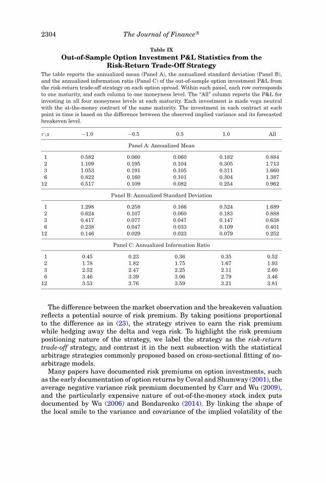
2304 The Journal of Finance R©
Table IXOut-of-Sample Option Investment P&L Statistics from the
Risk-Return Trade-Off StrategyThe table reports the annualized mean (Panel A), the annualized standard deviation (Panel B),and the annualized information ratio (Panel C) of the out-of-sample option investment P&L fromthe risk-return trade-off strategy on each option spread. Within each panel, each row correspondsto one maturity, and each column to one moneyness level. The “All” column reports the P&L forinvesting in all four moneyness levels at each maturity. Each investment is made vega neutralwith the at-the-money contract of the same maturity. The investment in each contract at eachpoint in time is based on the difference between the observed implied variance and its forecastedbreakeven level.
τ\x −1.0 −0.5 0.5 1.0 All
Panel A: Annualized Mean
1 0.582 0.060 0.060 0.182 0.8842 1.109 0.195 0.104 0.305 1.7133 1.053 0.191 0.105 0.311 1.6606 0.822 0.160 0.101 0.304 1.387
12 0.517 0.109 0.082 0.254 0.962
Panel B: Annualized Standard Deviation
1 1.298 0.258 0.166 0.524 1.6892 0.624 0.107 0.060 0.183 0.8883 0.417 0.077 0.047 0.147 0.6386 0.238 0.047 0.033 0.109 0.401
12 0.146 0.029 0.023 0.079 0.252
Panel C: Annualized Information Ratio
1 0.45 0.23 0.36 0.35 0.522 1.78 1.82 1.75 1.67 1.933 2.52 2.47 2.25 2.11 2.606 3.46 3.39 3.06 2.79 3.46
12 3.53 3.76 3.59 3.21 3.81
The difference between the market observation and the breakeven valuationreflects a potential source of risk premium. By taking positions proportionalto the difference as in (23), the strategy strives to earn the risk premiumwhile hedging away the delta and vega risk. To highlight the risk premiumpositioning nature of the strategy, we label the strategy as the risk-returntrade-off strategy, and contrast it in the next subsection with the statisticalarbitrage strategies commonly proposed based on cross-sectional fitting of no-arbitrage models.
Many papers have documented risk premiums on option investments, suchas the early documentation of option returns by Coval and Shumway (2001), theaverage negative variance risk premium documented by Carr and Wu (2009),and the particularly expensive nature of out-of-the-money stock index putsdocumented by Wu (2006) and Bondarenko (2014). By linking the shape ofthe local smile to the variance and covariance of the implied volatility of the
Option Profit and Loss Attribution and Pricing 2305
underlying option contract, our new theory allows us to identify a source of riskpremium based on the difference between the cross-sectional and time seriesestimates of these variance and covariance rates.
G.3. Statistical Arbitrage Trading Based on Cross-Sectional Fitting
A popular investment strategy commonly associated with no-arbitrage mod-els is statistical arbitrage trading based on the pricing errors of a cross-sectionally fitted no-arbitrage model.5 The idea underlying this strategy isto regard the pricing errors as temporal market mispricing and to form portfo-lios that are neutral to the risk factors of the model, so that the strategy doesnot take on the risk premiums of these risk factors, but bets purely on themean-reversion of the pricing errors.
To highlight the difference between the two types of investment strategies,we consider a statistical arbitrage trading strategy within the same contextof our risk-return trade-off investment exercise. Specifically, at each date andmaturity, we perform the following cross-sectional regression on the impliedvolatility smile within |x| ≤ 1:
St = γt(2z+) + ω2t (z+z−) + et. (24)
We have used this regression in equation (20) to estimate the risk-neutralvariance and covariance by assuming local commonality for moneyness within|x| ≤ 1. If our assumption is correct, the pricing errors from this cross-sectionalregression (et) can be regarded as temporary market mispricing and can betreated as statistical arbitrage opportunities. We set the weight invested ineach spread proportional to the pricing error,
wt = 10et/A2t . (25)
Different from the risk-return trade-off strategy, the weight for this statisticalarbitrage strategy does not depend on time series forecasts, but rather reliespurely on the pricing errors from the cross-sectional fitting. Although the twostrategies invest in the same spreads, their investment weights are based oncompletely different sources of information and assumptions.
As shown in Table VI, the local commonality assumption works well withinthe moneyness range, and this regression fits the smile extremely well. As aresult, the pricing errors are very small. We scale up the error by a magnitudeof 10 in equation (25), so that the absolute magnitudes of the weights are in asimilar range as those from the risk-return trade-off strategy.
Table X reports summary statistics for the investment weights on the sta-tistical arbitrage strategy. Via scaling, we have made the standard deviationand the minimum-maximum range of the investment weights to be of similar
5 Duarte, Longstaff, and Yu (2007) describe the performance of several common statistical ar-bitrage strategies in the fixed income market. Bali, Heidari, and Wu (2009) elaborate on theconstruction and performance of a statistical arbitrage trading strategy on the swap rate curvebased on pricing errors from multifactor dynamic term structure models.
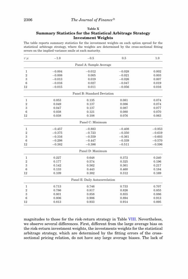
2306 The Journal of Finance R©
Table XSummary Statistics for the Statistical Arbitrage Strategy
Investment WeightsThe table reports summary statistics for the investment weights on each option spread for thestatistical arbitrage strategy, where the weights are determined by the cross-sectional fittingerrors on the implied variance smile at each maturity.
τ\x −1.0 −0.5 0.5 1.0
Panel A: Sample Average
1 −0.004 −0.012 −0.028 0.0022 −0.008 0.005 −0.021 0.0033 −0.013 0.019 −0.026 0.0076 −0.016 0.027 −0.047 0.019
12 −0.015 0.011 −0.056 0.016
Panel B: Standard Deviation
1 0.053 0.135 0.081 0.0742 0.049 0.137 0.086 0.0743 0.047 0.137 0.087 0.0776 0.038 0.121 0.080 0.070
12 0.038 0.108 0.076 0.063
Panel C: Minimum
1 −0.457 −0.883 −0.408 −0.8532 −0.375 −0.723 −0.350 −0.6193 −0.316 −0.559 −0.361 −0.6036 −0.298 −0.447 −0.339 −0.570
12 −0.382 −0.386 −0.511 −0.596
Panel D: Maximum
1 0.227 0.648 0.372 0.2402 0.177 0.574 0.325 0.1963 0.142 0.562 0.361 0.2176 0.133 0.443 0.460 0.184
12 0.109 0.382 0.312 0.169
Panel E: Daily Autocorrelation
1 0.713 0.746 0.733 0.7072 0.786 0.817 0.826 0.8553 0.801 0.858 0.855 0.8866 0.806 0.906 0.894 0.913
12 0.813 0.933 0.914 0.895
magnitudes to those for the risk-return strategy in Table VIII. Nevertheless,we observe several differences. First, different from the large average bias onthe risk-return investment weights, the investments weights for the statisticalarbitrage strategy, which are determined by the fitting errors of the cross-sectional pricing relation, do not have any large average biases. The lack of
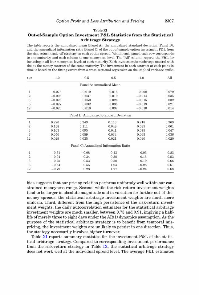
Option Profit and Loss Attribution and Pricing 2307
Table XIOut-of-Sample Option Investment P&L Statistics from the Statistical
Arbitrage StrategyThe table reports the annualized mean (Panel A), the annualized standard deviation (Panel B),and the annualized information ratio (Panel C) of the out-of-sample option investment P&L fromthe risk-return trade-off strategy on each option spread. Within each panel, each row correspondsto one maturity, and each column to one moneyness level. The “All” column reports the P&L forinvesting in all four moneyness levels at each maturity. Each investment is made vega neutral withthe at-the-money contract of the same maturity. The investment in each contract at each point intime is based on the fitting errors from a cross-sectional regression on the implied variance smile.
τ\x −1.0 −0.5 0.5 1.0 All
Panel A: Annualized Mean
1 0.075 −0.019 0.015 0.008 0.0792 −0.006 0.037 0.019 −0.014 0.0353 −0.026 0.050 0.024 −0.015 0.0326 −0.027 0.032 0.035 −0.019 0.021
12 −0.023 0.010 0.037 −0.010 0.014
Panel B: Annualized Standard Deviation
1 0.220 0.249 0.113 0.218 0.3692 0.138 0.111 0.048 0.085 0.0613 0.103 0.095 0.041 0.075 0.0476 0.050 0.059 0.034 0.065 0.036
12 0.029 0.035 0.021 0.040 0.020
Panel C: Annualized Information Ratio
1 0.31 −0.08 0.13 0.03 0.232 −0.04 0.34 0.38 −0.15 0.533 −0.25 0.53 0.58 −0.19 0.666 −0.54 0.55 1.04 −0.28 0.61
12 −0.79 0.28 1.77 −0.24 0.68
bias suggests that our pricing relation performs uniformly well within our con-strained moneyness range. Second, while the risk-return investment weightstend to be larger in absolute magnitude and in variation for further out-of-the-money spreads, the statistical arbitrage investment weights are much moreuniform. Third, different from the high persistence of the risk-return invest-ment weights, the daily autocorrelation estimates for the statistical arbitrageinvestment weights are much smaller, between 0.73 and 0.91, implying a half-life of merely three to eight days under the AR(1) dynamics assumption. As thepurpose of the statistical arbitrage strategy is to benefit from temporal mis-pricing, the investment weights are unlikely to persist in one direction. Thus,the strategy necessarily involves higher turnover.
Table XI reports summary statistics for the investment P&L of the statis-tical arbitrage strategy. Compared to corresponding investment performancefrom the risk-return strategy in Table IX, the statistical arbitrage strategydoes not work well at the individual spread level. The average P&L estimates
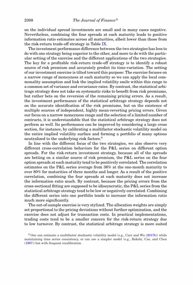
2308 The Journal of Finance R©
on the individual spread investments are small and in many cases negative.Nevertheless, combining the four spreads at each maturity leads to positiveinformation ratio estimates across all maturities, albeit lower than those fromthe risk-return trade-off strategy in Table IX.
The investment performance difference between the two strategies has less todo with one strategy being superior to the other, and more to do with the partic-ular setting of the exercise and the different applications of the two strategies.The key for a profitable risk-return trade-off strategy is to identify a robustsource of risk premium and accurately predict its time-variation. The settingof our investment exercise is tilted toward this purpose: The exercise focuses ona narrow range of moneyness at each maturity so we can apply the local com-monality assumption and link the implied volatility smile within this range toa common set of variance and covariance rates. By contrast, the statistical arbi-trage strategy does not take on systematic risks to benefit from risk premiums,but rather bets on the reversion of the remaining pricing errors. As a result,the investment performance of the statistical arbitrage strategy depends noton the accurate identification of the risk premiums, but on the existence ofmultiple sources of independent, highly mean-reverting pricing errors. Givenour focus on a narrow moneyness range and the selection of a limited number ofcontracts, it is understandable that the statistical arbitrage strategy does notperform as well. Its performance can be improved by considering a large crosssection, for instance, by calibrating a multifactor stochastic volatility model onthe entire implied volatility surface and forming a portfolio of many optionsneutralized to the underlying risk factors.6
In line with the different focus of the two strategies, we also observe verydifferent cross-correlation behaviors for the P&L series on different optionspreads. For the risk-return investment strategy, because all of the spreadsare betting on a similar source of risk premium, the P&L series on the fouroption spreads at each maturity tend to be positively correlated. The correlationestimates on the P&L series average from 36% at the one-month maturity toover 80% for maturities of three months and longer. As a result of the positivecorrelation, combining the four spreads at each maturity does not increasethe information ratio much. By contrast, because the pricing errors from thecross-sectional fitting are supposed to be idiosyncratic, the P&L series from thestatistical arbitrage strategy tend to be low or negatively correlated. Combiningthe different series into one portfolio tends to increase the information ratiomuch more significantly.
The out-of-sample exercise is very stylized. The allocation weights are simplyset proportional to the pricing deviations without further optimization, and theexercise does not adjust for transaction costs. In practical implementations,trading costs tend to be a smaller concern for the risk-return strategy dueto low turnover. By contrast, the statistical arbitrage strategy is more suited
6 One can estimate a multifactor stochastic volatility model (e.g., Carr and Wu (2017b)) whilemaintaining time series consistency, or can use a simpler model (e.g., Bakshi, Cao, and Chen(1997)) but with frequent recalibration.
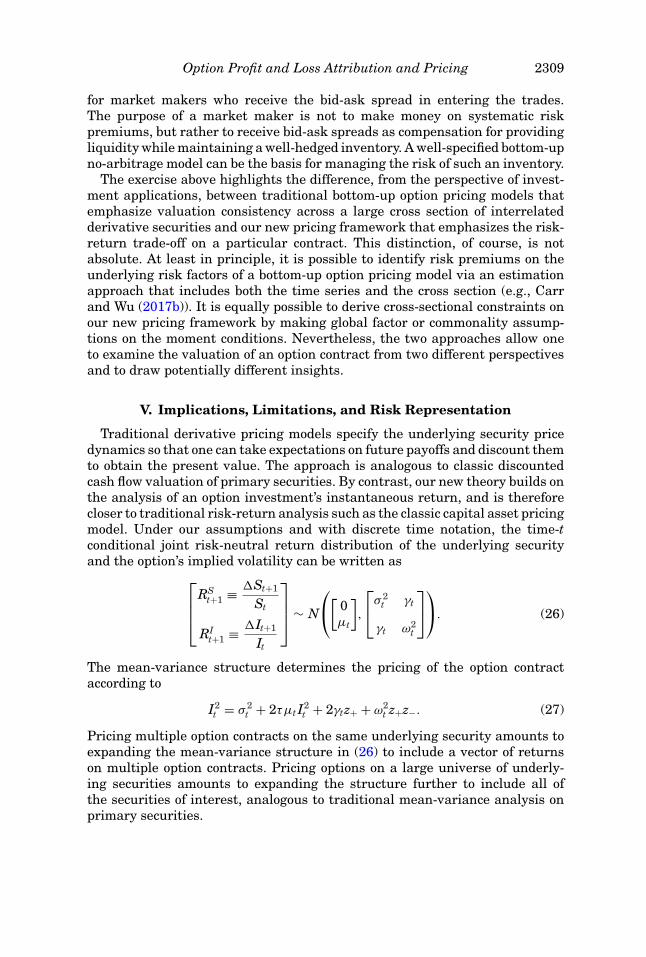
Option Profit and Loss Attribution and Pricing 2309
for market makers who receive the bid-ask spread in entering the trades.The purpose of a market maker is not to make money on systematic riskpremiums, but rather to receive bid-ask spreads as compensation for providingliquidity while maintaining a well-hedged inventory. A well-specified bottom-upno-arbitrage model can be the basis for managing the risk of such an inventory.
The exercise above highlights the difference, from the perspective of invest-ment applications, between traditional bottom-up option pricing models thatemphasize valuation consistency across a large cross section of interrelatedderivative securities and our new pricing framework that emphasizes the risk-return trade-off on a particular contract. This distinction, of course, is notabsolute. At least in principle, it is possible to identify risk premiums on theunderlying risk factors of a bottom-up option pricing model via an estimationapproach that includes both the time series and the cross section (e.g., Carrand Wu (2017b)). It is equally possible to derive cross-sectional constraints onour new pricing framework by making global factor or commonality assump-tions on the moment conditions. Nevertheless, the two approaches allow oneto examine the valuation of an option contract from two different perspectivesand to draw potentially different insights.
V. Implications, Limitations, and Risk Representation
Traditional derivative pricing models specify the underlying security pricedynamics so that one can take expectations on future payoffs and discount themto obtain the present value. The approach is analogous to classic discountedcash flow valuation of primary securities. By contrast, our new theory builds onthe analysis of an option investment’s instantaneous return, and is thereforecloser to traditional risk-return analysis such as the classic capital asset pricingmodel. Under our assumptions and with discrete time notation, the time-tconditional joint risk-neutral return distribution of the underlying securityand the option’s implied volatility can be written as⎡⎢⎢⎣
RSt+1 ≡ St+1
St
RIt+1 ≡ It+1
It
⎤⎥⎥⎦ ∼ N
⎛⎝[ 0μt
],
⎡⎣σ 2t γt
γt ω2t
⎤⎦⎞⎠. (26)
The mean-variance structure determines the pricing of the option contractaccording to
I2t = σ 2
t + 2τμt I2t + 2γtz+ + ω2
t z+z−. (27)
Pricing multiple option contracts on the same underlying security amounts toexpanding the mean-variance structure in (26) to include a vector of returnson multiple option contracts. Pricing options on a large universe of underly-ing securities amounts to expanding the structure further to include all ofthe securities of interest, analogous to traditional mean-variance analysis onprimary securities.
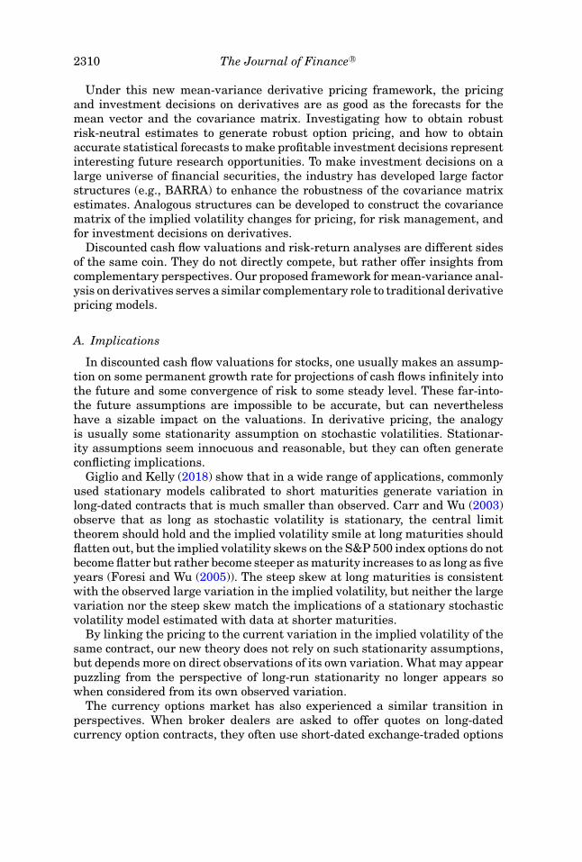
2310 The Journal of Finance R©
Under this new mean-variance derivative pricing framework, the pricingand investment decisions on derivatives are as good as the forecasts for themean vector and the covariance matrix. Investigating how to obtain robustrisk-neutral estimates to generate robust option pricing, and how to obtainaccurate statistical forecasts to make profitable investment decisions representinteresting future research opportunities. To make investment decisions on alarge universe of financial securities, the industry has developed large factorstructures (e.g., BARRA) to enhance the robustness of the covariance matrixestimates. Analogous structures can be developed to construct the covariancematrix of the implied volatility changes for pricing, for risk management, andfor investment decisions on derivatives.
Discounted cash flow valuations and risk-return analyses are different sidesof the same coin. They do not directly compete, but rather offer insights fromcomplementary perspectives. Our proposed framework for mean-variance anal-ysis on derivatives serves a similar complementary role to traditional derivativepricing models.
A. Implications
In discounted cash flow valuations for stocks, one usually makes an assump-tion on some permanent growth rate for projections of cash flows infinitely intothe future and some convergence of risk to some steady level. These far-into-the future assumptions are impossible to be accurate, but can neverthelesshave a sizable impact on the valuations. In derivative pricing, the analogyis usually some stationarity assumption on stochastic volatilities. Stationar-ity assumptions seem innocuous and reasonable, but they can often generateconflicting implications.
Giglio and Kelly (2018) show that in a wide range of applications, commonlyused stationary models calibrated to short maturities generate variation inlong-dated contracts that is much smaller than observed. Carr and Wu (2003)observe that as long as stochastic volatility is stationary, the central limittheorem should hold and the implied volatility smile at long maturities shouldflatten out, but the implied volatility skews on the S&P 500 index options do notbecome flatter but rather become steeper as maturity increases to as long as fiveyears (Foresi and Wu (2005)). The steep skew at long maturities is consistentwith the observed large variation in the implied volatility, but neither the largevariation nor the steep skew match the implications of a stationary stochasticvolatility model estimated with data at shorter maturities.
By linking the pricing to the current variation in the implied volatility of thesame contract, our new theory does not rely on such stationarity assumptions,but depends more on direct observations of its own variation. What may appearpuzzling from the perspective of long-run stationarity no longer appears sowhen considered from its own observed variation.
The currency options market has also experienced a similar transition inperspectives. When broker dealers are asked to offer quotes on long-datedcurrency option contracts, they often use short-dated exchange-traded options
Option Profit and Loss Attribution and Pricing 2311
as a starting point and perform extrapolation. In early years, the commonpractice was to flat-extrapolate the at-the-money option implied volatility fromshort to long maturities when there was no additional information about thelong-run behavior. To extrapolate the implied volatilities of out-of-the-moneyoptions, broker dealers and quantitative researchers recognized the effect ofthe central limit theorem, which led them to quote increasingly flatter impliedvolatility smiles as the extrapolated maturity increased. Years of investmentexperiences, however, has made them realize the inadequacy and inconsistencyof such an extrapolation approach. Since the early 2000s, the common practicehas shifted to extrapolating the entire implied volatility smile shape instead ofjust the at-the-money implied volatility level. The new extrapolation approachimplies that the risk-neutral return skewness and kurtosis stay the same asthe conditional horizon increases. This extrapolation seems to run againstthe central limit theorem. However, out of the two approaches, only the morerecent approach is consistent with the implication of our new theory: If oneflat-extrapolates the at-the-money implied volatility from one year to 10 years,both the variation and the covariation of the 10-year implied volatility willbe identical to those of the one-year implied volatility, and our new pricingtheory suggests that the two maturities must share the same implied volatilitysmile shape as well. The implication of the central limit theorem based onstationarity assumptions cannot kick in as long as the variation in the impliedvolatility remains large.
B. Limitations
Mean-variance analysis has been the pillar of modern finance. Our new the-ory can become the stepping stone for expanding mean-variance analysis toderivative securities. However, the mean-variance framework fails to accountfor the presence of rare but large events (jumps). The literature includes nu-merous efforts to integrate jumps into mean-variance analysis for both pricingand investment decisions on primary securities. Future research could examinehow to integrate jumps into our new framework for derivative pricing.
In many cases, incorporating jumps results in complications that make theanalysis lose its original clarity and appeal. In such cases, instead of compli-cating the analysis via integration, one can follow the same spirit that ournew theory advocates and decentralize, analyzing normal-day behavior via thesimple mean-variance structure while analyzing rare, large events separatelyvia scenario analysis and stress tests.
C. Risk Representation
In deriving our pricing equation for a vanilla option contract, we use theBMS model to transform the option price into the BMS implied volatility asa representation of the option contract’s main risk sources, analogous to thecommon practice in the fixed income market of transforming bond prices intoyield to maturities to highlight the underlying interest rate risk.
2312 The Journal of Finance R©
Traditional option pricing models represent the risk of many option contractsvia a few global risk factors. To generate localized pricing implications, werequire that the risk representation be local to the particular option contract.Just as yield to maturity is local to the particular coupon bond, so is impliedvolatility local to the particular option contract. Accordingly, in choosing aparticular form of risk representation for our purpose, the first requirement isthat the transformation be a local, unique, monotone, and one-to-one mappingto the option price. For this purpose, the local volatility model of Dupire (1994)or stochastic volatility models such as Heston (1993) are not good candidates.
The second requirement is that the transformed quantities become more sta-ble and more comparable across contracts and over time than the raw contractprices. For bonds, if the instantaneous interest rate is constant, yield to matu-rity across all bonds will be the same. For options, if the security price follows adiffusive process with a constant instantaneous return volatility, the BMS im-plied volatility will be the same across all option contracts underlying the samesecurity. This analogous feature allows the yield and the implied volatility tobe both somewhat stable and comparable across contracts and over time. Justas yields of nearby maturities tend to be similar and move together by natureof arbitrage trading, so do implied volatilities of option contracts at nearbystrikes and maturities.
A third requirement is ease of interpretation in that the transformed quanti-ties have some specific and intuitive economic meaning, at least under certainmodel environments. The yield to maturity has the economic interpretation ofbeing the return to the bond investment if one buys the bond at the currentprice and holds the bond to maturity assuming no default. The BMS impliedvolatility has the economic interpretation of being the security return volatilityunder the BMS model environment. More generally, under continuous price dy-namics, the BMS implied variance represents the risk-neutral expected valueof the integrated future instantaneous return variance weighted by the BMSgamma along the sample path.
Nevertheless, it is important to emphasize that although the BMS formularepresents a very intuitive and simple representation of an option contract’sunderlying risk sources, one can explore other transformations that may repre-sent the underlying risk sources even better. As an example, a recent workingpaper by Shue and Townsend (2018) suggests that people tend to think ad-ditively instead of multiplicatively, so that stock price movements look morearithmetic than geometric. If this is indeed the case, an alternative representa-tion would be the Bachelier’s (1900) model, under which one measures volatilityon price changes instead of percentage returns.
Finally, this paper uses the option contract as an example and uses thewell-adopted BMS implied volatility as the transformation. For other financialcontracts, it is natural to find the risk representation that best suits the par-ticular contracts under consideration. As we discuss above, if the analysis is oncoupon bonds, the yield-to-maturity transformation will be the natural choice(Carr and Wu (2017a)).
Option Profit and Loss Attribution and Pricing 2313
VI. Concluding Remarks
We develop a new option pricing framework based on the P&L attributionanalysis of option investments. The analysis starts with the Black-Merton-Scholes option pricing equation and attributes the instantaneous return of anoption investment to calendar decay, to changes in the underlying securityprice, to changes in the option’s implied volatility, and to higher order effects.Taking risk-neutral expectation and applying dynamic no-arbitrage constraintsresults in a pricing relation that links the option’s fair implied volatility level tothe implied volatility’s own expected direction of movement, its variance, andits covariance with the security return. The valuation does not need to specifywhere the first- and second-moment conditions come from or how they vary inthe future, thus allowing us to make top-down, localized valuations based onwhat we know best about the particular contract.
The top-down perspective does not preclude us from making either local com-monality assumptions on the implied volatility co-movements across nearbyoption contracts, or global commonality assumptions based on principal com-ponent analysis or some other factor structures. Imposing these commonalityassumptions on our pricing equation leads to cross-sectional pricing implica-tions either for a select number or range of contracts or for the entire im-plied volatility surface.
By shifting the focus from terminal payoffs to short-term P&L fluctuations,our new theory not only provides simple and flexible pricing solutions forderivative contracts of interest, but also tightly links the pricing to risk manage-ment practices, and provides a foundation for expanding classic mean-variancerisk-return analysis to derivative contracts.
In future research, one could expand existing return factor structures onprimary securities by developing analogous factor structures on the impliedvolatility changes of the underlying option contracts. The joint return/impliedvolatility factor structure has direct pricing implications for the option con-tracts, making it suitable as the foundation for investment analysis onthe expanded universe that includes both primary securities and derivativecontracts.
Initial submission: April 23, 2018; Accepted: October 16, 2019Editors: Stefan Nagel, Philip Bond, Amit Seru, and Wei Xiong
Appendix: BMS Sensitivities
The standard greeks of the BMS model are well known and are availablein standard textbooks, such as Chapter 17 in Hull (2009). A call option’s BMSdelta is given by
BS = N(d1), d1 = ln St/K + 12 I2
t τ
It√
τ= − z−
It√
τ, (A1)
2314 The Journal of Finance R©
where N(·) is the cumulative normal function. The BMS gamma is
BSS = n(d1)St It
√τ
, (A2)
where n(·) denotes the probability density function of the standard normalvariable. The cash gamma BSSS2
t is therefore
BSSS2t = Stn(d1)
It√
τ. (A3)
All other sensitivity measures of interest can be represented in terms of thecash gamma. The BMS theta is
Bt = −12
Stn(d1)It/√
τ = −12
I2t BSSS2
t . (A4)
The BMS vega is
BI = St√
τn(d1), (A5)
so the cash vega BI It can be represented by
BI It = St It√
τn(d1) = I2t τ BSSS2
t . (A6)
Vanna and volga are not in standard textbooks but can be derived just as easily.The vanna is
BIS = ∂ BI
∂St= √
τn(d1) − d1n(d1)/It, (A7)
so the dollar vanna BIS ItSt can be represented by
BIS ItSt = Stn(d1)(It√
τ − d1) = Stn(d1)It√
τ
(ln K/St + 1
2I2t τ
)= BSSS2
t z+. (A8)
Finally, the volga is
BII = ∂ BI
∂ It= St
√τn(d1)(−d1)
(− ln St/K
I2t√
τ+ 1
2√
τ
), (A9)
so the dollar volga BII I2t can be represented by
BII I2t = Stn(d1)(−d1)
(− ln St/K + 1
2I2t τ
)= BSSS2
t z−z+. (A10)
REFERENCES
An, Byeong-Je, Andrew Ang, Turan G. Bali, and Nusret Cakici, 2014, The joint cross section ofstocks and options, Journal of Finance 69, 2279–2337.
Option Profit and Loss Attribution and Pricing 2315
Arrow, Kenneth J., and Gerard Debreu, 1954, Existence of an equilibrium for a competitive econ-omy, Econometrica 22, 265–290.
Arslan, Melih, Gilbert Eid, Jean El Khoury, and Jason Roth, 2009, The gamma vanna volga costframework for constructing implied volatility curves, Working paper, Deutsche Bank.
Avellaneda, Marco, and Yingzi Zhu, 1998, A risk-neutral stochastic volatility model, InternationalJournal of Theoretical and Applied Finance 1, 289–310.
Bachelier, Louis, 1900, Theorie de la speculation, Ph.D. thesis Paris.Bakshi, Gurdip, Charles Cao, and Zhiwu Chen, 1997, Empirical performance of alternative option
pricing models, Journal of Finance 52, 2003–2049.Bakshi, Gurdip, and Dilip Madan, 2000, Spanning and derivative-security valuation, Journal of
Financial Economics 55, 205–238.Bali, Turan, Massoud Heidari, and Liuren Wu, 2009, Predictability of interest rates and interest-
rate portfolios, Journal of Business and Economic Statistics 27, 517–527.Bergomi, Lorenzo, 2016, Stochastic Volatility Modeling (CRC Press, Boca Raton, FL).Black, Fisher, and Myron Scholes, 1973, The pricing of options and corporate liabilities, Journal
of Political Economy 81, 637–654.Bondarenko, Oleg, 2014, Why are put options so expensive? Quarterly Journal of Finance 4, 1–50.Boyer, Brian H., and Keith Vorkink, 2014, Stock options as lotteries, Journal of Finance 69, 1485–
1527.Byun, Suk-Joon, and Da-Hea Kim, 2016, Gambling preference and individual equity option returns,
Journal of Financial Economics 122, 155–174.Carr, Peter, and Liuren Wu, 2003, Finite moment log stable process and option pricing, Journal of
Finance 58, 753–777.Carr, Peter, and Liuren Wu, 2009, Variance risk premiums, Review of Financial Studies 22, 1311–
1341.Carr, Peter, and Liuren Wu, 2010, Stock options and credit default swaps: A joint framework for
valuation and estimation, Journal of Financial Econometrics 8, 409–449.Carr, Peter, and Liuren Wu, 2017a, Decomposing long bond returns: A decentralized modeling
approach, Working paper, New York University and Baruch College.Carr, Peter, and Liuren Wu, 2017b, Leverage effect, volatility feedback, and self-exciting market
disruptions, Journal of Financial and Quantitative Analysis 52, 2119–2156.Castagna, Antonio, and Fabio Mercurio, 2007, The vanna-volga method for implied volatilities,
Risk , 1, 106–111.Coval, Joshua D., and Tyler Shumway, 2001, Expected option returns, Journal of Finance 56,
983–1009.Daglish, Toby, John Hull, and Wulin Suo, 2007, Volatility surfaces: Theory, rules of thumb, and
empirical evidence, Quantitative Finance 7, 507–524.Driessen, Joost, Pascal J. Maenhout, and Grigory Vilkov, 2009, The price of correlation risk:
Evidence from equity options, Journal of Finance 64, 1377–1406.Duarte, Jefferson, Francis A. Longstaff, and Fan Yu, 2007, Risk and return in fixed income arbi-
trage: Nickels in front of a streamroller, Review of Financial Studies 20, 769–811.Dupire, Bruno, 1994, Pricing with a smile, Risk 7, 18–20.Egloff, Daniel, Markus Leippold, and Liuren Wu, 2010, The term structure of variance swap rates
and optimal variance swap investments, Journal of Financial and Quantitative Analysis 45,1279–1310.
Fengler, Matthias R., 2005, Semiparametric Modeling of Implied Volatility. (Springer, Berlin).Foresi, Silverio, and Liuren Wu, 2005, Crash-o-phobia: A domestic fear or a worldwide concern?
Journal of Derivatives 13, 8–21.Gershon, David, 2018, Model independent multi-asset volatility smile with empirical confirmation,
Working paper, Hebrew University of Jerusalem.Giglio, Stefano, and Bryan T. Kelly, 2018, Excess volatility: Beyond discount rates, Quarterly
Journal of Economics 133, 71–127.Hafner, Reinhold, 2004, Stochastic Implied Volatility: A Factor-Based Model. (Springer, Berlin).Heath, David, Robert Jarrow, and Andrew Morton, 1992, Bond pricing and the term structure of
interest rates: A new technology for contingent claims valuation, Econometrica 60, 77–105.
2316 The Journal of Finance R©
Heston, Steven L., 1993, Closed-form solution for options with stochastic volatility, with applicationto bond and currency options, Review of Financial Studies 6, 327–343.
Hodges, Hardy M., 1996, Arbitrage bounds of the implied volatility strike and term structures ofEuropean-style options, Journal of Derivatives 3, 23–32.
Hu, Guanglian, and Kris Jacobs, 2017, Volatility and expected option returns, Working paper,University of Houston.
Hull, John C., 2009, Options, Futures, and Other Derivatives (Pearson Prentice Hall, New York).Israelov, Roni, and Bryan T. Kelly, 2017, Forecasting the distribution of option returns, Working
paper, AQR and University of Chicago.Jones, Christopher S., 2006, A nonlinear factor analysis of S&P 500 index option returns, Journal
of Finance 61, 2325–2363.Merton, Robert C., 1973, Theory of rational option pricing, Bell Journal of Economics and Man-
agement Science 4, 141–183.Newey, Whitney K., and Kenneth D. West, 1987, A simple, positive semi-definite, heteroskedastic-
ity and autocorrelation consistent covariance matrix, Econometrica 55, 703–708.Schonbucher, Philipp J., 1999, A market model for stochastic implied volatility, Philosophical
Transactions: Mathematical, Physical and Engineering Sciences 357, 2071–2092.Shue, Kelly, and Tichard R. Townsend, 2018, Can the market multiply and divide? non-proportional
thinking in financial markets, Working paper, Yale University and UC San Diego.Wu, Liuren, 2006, Dampened power law: Reconciling the tail behavior of financial asset returns,
Journal of Business 79, 1445–1474.Wu, Liuren, and Jingyi Zhu, 2016, Simple robust hedging with nearby contracts, Journal of Fi-
nancial Econometrics 15, 1–35.Wystup, Uwe, 2010, Vanna-volga pricing, in Rama Cont, ed.: Encyclopedia of Quantitative Finance
(John Wiley & Sons, Chichester).
Supporting Information
Additional Supporting Information may be found in the online version of thisarticle at the publisher’s website:
Replication code.