GSK3 Я phosphorylation modulates CLASP – microtubule association and lamella microtubule
Upload
truonglienCategory
view
216download
1
OPTIMUM TOPOLOGICAL DESIGN OF GEOMETRICALLY
NONLINEAR SINGLE LAYER LAMELLA DOMES USING
HARMONY SEARCH METHOD
A THESIS SUBMITTED TO
THE GRADUATE SCHOOL OF NATURAL AND APPLIED SCIENCES
OF
MIDDLE EAST TECHNICAL UNIVERSITY
BY
SERDAR ÇARBAġ
IN PARTIAL FULFILLMENT OF THE REQUIREMENTS
FOR
THE DEGREE OF MASTER OF SCIENCE
IN
ENGINEERING SCIENCES
JULY 2008

Approval of the thesis:
OPTIMUM TOPOLOGICAL DESIGN OF GEOMETRICALLY
NONLINEAR SINGLE LAYER LAMELLA DOMES USING
HARMONY SEARCH METHOD
Submitted by SERDAR ÇARBAŞ in partial fulfillment of the requirements for the
degree of Master of Science in Engineering Sciences Department, Middle East
Technical University by,
Prof. Dr. Canan Özgen ________________
Dean, Graduate School of Natural and Applied Sciences
Prof. Dr. Turgut Tokdemir ________________
Head of Department, Engineering Sciences
Prof. Dr. Mehmet Polat Saka ________________
Supervisor, Engineering Sciences Dept., METU
Examining Committee Members:
Prof. Dr. Mehmet Polat Saka ________________
Engineering Sciences Dept., METU
Prof. Dr. Gülin AyĢe Birlik ________________
Engineering Sciences Dept., METU
Assoc. Prof. Dr. Murat Dicleli ________________
Engineering Sciences Dept., METU
Assist. Prof. Dr. Oğuzhan Hasançebi ________________
Civil Engineering Dept., METU
Assist. Prof. Dr. M. Tolga Yılmaz ________________
Engineering Sciences Dept., METU
Date: July 03, 2008

iii
I hereby declare that all information in this document has been obtained and
presented in accordance with academic rules and ethical conduct. I also declare
that, as required by these rules and conduct, I have fully cited and referenced all
material and results that are not original to this work.
Name, Last name : Serdar ÇarbaĢ
Signature :

iv
ABSTRACT
OPTIMUM TOPOLOGICAL DESIGN OF GEOMETRICALLY
NONLINEAR SINGLE LAYER LAMELLA DOMES USING
HARMONY SEARCH METHOD
ÇarbaĢ, Serdar
M.S., Department of Engineering Sciences
Supervisor: Prof. Dr. Mehmet Polat Saka
July 2008, 118 pages
Harmony search method based optimum topology design algorithm is
presented for single layer lamella domes. The harmony search method is a
numerical optimization technique developed recently that imitates the musical
performance process which takes place when a musician searches for a better
state of harmony. Jazz improvisation seeks to find musically pleasing harmony
similar to the optimum design process which seeks to find the optimum
solution. The optimum design algorithm developed imposes the behavioral and
performance constraints in accordance with LRFD-AISC. The optimum
number of rings, the height of the crown and the tubular cross-sectional
designations for dome members are treated as design variables. The member
grouping is allowed so that the same section can be adopted for each group.
The design algorithm developed has a routine that build the data for the
geometry of the dome automatically that covers the numbering of joints, and
member incidences, and the computation of the coordinates of joints. Due to
the slenderness and the presence of imperfections in dome structures it is
necessary to consider the geometric nonlinearity in the prediction of their
response under the external loading. Design examples are considered to
demonstrate the efficiency of the algorithm presented.

v
Keywords: Optimum Structural Design, Harmony Search Algorithm,
Minimum Weight, Stochastic Search Technique, Lamella Domes.

vi
ÖZ
HARMONĠ ARAMA YÖNTEMĠ KULLANILARAK GEOMETRĠK
YÖNDEN DOĞRUSAL OLMAYAN TEK KATMANLI YAPRAKSI
KUBBELERĠN OPTĠMUM TOPOLOJĠ BOYUTLANDIRMASI
ÇarbaĢ, Serdar
Yüksek Lisans, Mühendislik Bilimleri Bölümü
Tez Yöneticisi: Prof. Dr. Mehmet Polat Saka
Temmuz 2008, 118 sayfa
Tek katmanlı yapraksı kubbeler için harmoni arama yöntemine dayalı optimum
topoloji tasarım algoritması sunulmaktadır. Bir müzisyenin daha iyi bir
müzikal sunum arayıĢı içinde uygulamaya çalıĢtığı müzikal performans
sürecine benzetilen harmoni arama yöntemi yakın geçmiĢte geliĢtirilen bir
sayısal optimizasyon tekniğidir. Caz doğaçlaması, optimum çözüme ulaĢmaya
çalıĢan optimum tasarım sürecine benzer Ģekilde, müzikal açıdan tatmin edici
uyumu bulmaya çabalar. GeliĢtirilen optimum tasarım algoritması, LRFD-
AISC (Load and Resistance Factor Design-American Institute of Steel
Construction)„ye uygun olan davranıĢ ve performans sınırlayıcılarını uygular.
Optimum halka sayısı, tepe yüksekliği ve boru Ģeklindeki kesitler kubbe için
tasarım değiĢkenleridir. Her grupta aynı kesitlerin seçilebilmesi için eleman
gruplandırmasına izin verilmiĢtir. GeliĢtirilen tasarım algoritması, bağlantı
noktalarının ve eleman numaralandırılmalarının ve bağlantı noktalarının
koordinat hesaplarının otomatik olarak yapılmasını kapsayan, kubbenin
geometrik verilerini oluĢturan bir yordama sahiptir. Kubbe yapılarda,

vii
narinlikten ve kusurların var olmasından dolayı bu yapıların dıĢ yükler altında
vereceği tepkiyi tahmin ederken geometrik doğrusalsızlığı göz önüne almak
gerekmektedir. Dikkate alınan tasarım örnekleri sunulan algoritmanın
etkinliğini göstermeyi amaçlamaktadır.
Anahtar Kelimeler: Optimum Yapısal Tasarım, Harmoni Arama Yöntemi,
Minimum Ağırlık, Stokastik Arama Tekniği, Yapraksı Kubbeler.

viii
To My Family,
For your endless support and love

ix
ACKNOWLEDGEMENTS
I wish to offer my sincere thanks and appreciation to my supervisor
Prof. Dr. Mehmet Polat Saka for his precious help, invaluable suggestions,
continuous support, guidance, criticisms, encouragements and patience
throughout this study.
Secondly, I would like to thank Prof. Dr. M. RuĢen Geçit for his helpful
advices and avuncular humanity to me during my work life at Department of
Engineering Sciences.
My special thanks are due to Prof. Dr. Temel Yetimoğlu from Atatürk
University Engineering Faculty Civil Engineering Department for his great
encouragement in performing this research.
I should remark that without the sincere friendship of my roommate Semih
Erhan, this work would not have been realized. I strongly thank him for his
amity. And many thanks to Ferhat Erdal, Erkan Doğan, Alper Akın, and
Ġbrahim Aydoğdu for their excellent understanding and no end of aid at every
stage of my thesis study.
I would also like to thank to my friends, especially Hakan Bayrak, Refik Burak
TaymuĢ, Fuat Korkut, Hüseyin Çelik and Kaveh Hassanzehtap for their
friendship and encouragement during this study.
I owe thanks to most special person in my life Buket Bezgin and her housemate
Yasemin Çetin for their boundless moral support giving me joy of living.

x
Last but not least, I can hardly find words to express my feelings about my
parents Süreyya and Hayriye ÇarbaĢ, and my unique elder sister AyĢegül for
their lifetime support to compensate all the disadvantages in my life. I will
always be indebted to their compassion and humanism no matter how hard I try
to give back what they have given to me. They have priceless meaning for me.
I feel very lucky to have such a family.

xi
TABLE OF CONTENTS
ABSTRACT …………………………………………………………….... iv
ÖZ…………………………………………………………………………. vi
ACKNOWLEDGEMENTS……………………………………………...... ix
TABLE OF CONTENTS………………………………………………..... xi
LIST OF FIGURES……………………………………………………... xiv
LIST OF TABLES ……………………..........................................….... xvi
1.INTRODUCTION ........................................................................................ 1
1.1 Domes ....................................................................................................... 1
1.1.1 Types of Braced Domes ...................................................................... 4
1.2 Optimization in Engineering ...................................................................... 6
1.3 Structural Optimization ............................................................................. 8
1.3.1 Mathematical Modeling of Structural Optimization Problems ............. 9
1.3.2 Methods of Structural Optimization .................................................. 10
1.3.2.1 Analytical Methods..................................................................... 11
1.3.2.2 Numerical Methods .................................................................... 11
1.4 Stochastic Optimization Techniques ........................................................ 13
1.4.1 Genetic Algorithms ........................................................................... 14
1.4.2 Evolutionary Strategies ..................................................................... 15
1.4.3 Simulated Annealing ......................................................................... 15
1.4.4 Particle Swarm Optimization............................................................. 16
1.4.5 Ant Colony Optimization .................................................................. 17
1.4.6 Tabu Search ...................................................................................... 18
1.4.7 Harmony Search Optimization .......................................................... 19

xii
1.5 Literature Survey on the Optimum Design of Dome Structures ................ 20
1.6 The Scope of This Study .......................................................................... 26
2.ELASTIC-CRITICAL LOAD ANALYSIS OF SPATIAL STRUCTURES 28
2.1 Definition of Elastic Critical Load Analysis ............................................. 28
2.2 Calculation of Elastic Critical Load Factor .............................................. 29
2.3 Stiffness Matrix of a Space Member ........................................................ 30
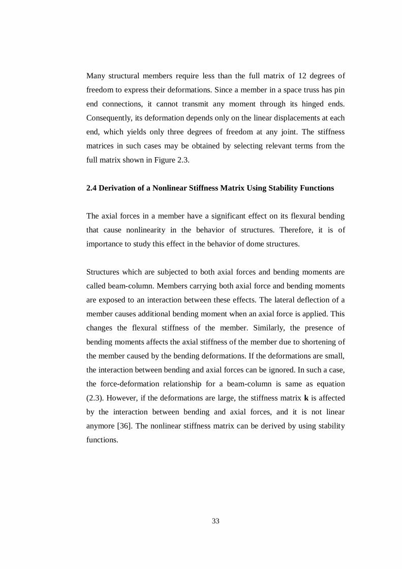
2.4 Derivation of a Nonlinear Stiffness Matrix Using Stability Functions ...... 33
2.4.1 Stability Functions ............................................................................ 34
2.4.1.1 Effect of Flexure on Axial Stiffness ............................................ 35
2.4.1.2 Effect of Axial Force on Flexural Stiffness ................................. 41
2.4.1.2.1 Bending in X-Y Plane ........................................................... 41
2.4.1.2.2 Bending in X-Z Plane ........................................................... 42
2.4.1.3 Effect of Axial Force on Stiffness Against Translation................ 43
2.4.1.3.1 Translation in X-Y Plane ....................................................... 43
2.4.1.3.2 Translation in X-Z Plane ....................................................... 46
2.5 Geometric Nonlinearity ........................................................................... 49
2.5.1 Construction of Overall Stiffness Matrix ........................................... 49
2.6 Elastic Critical Load Analysis .................................................................. 59
3.OPTIMUM DESIGN OF LAMELLA DOMES .......................................... 63
3.1 Morphology of Lamella Domes ............................................................... 63
3.2 Optimum Topology Design of Lamella Domes ........................................ 68
3.3 Mathematical Model of Optimum Design Problem of Lamella Domes
According to LRFD-AISC ............................................................................. 71

xiii
4.HARMONY SEARCH METHOD BASED OPTIMUM DESIGN
ALGORITHM............................................................................................... 75
4.1 General Concept of Harmony Search Algorithm ...................................... 75
4.2 A Harmony Search Algorithm Based Optimum Design Method For Single
Layer Lamella Domes ................................................................................... 81
5.DESIGN EXAMPLES ............................................................................... 88
5.1 CASE 1 (P) ............................................................................................. 90
5.2 CASE 2 ( D + P ) ..................................................................................... 96
5.3 CASE 3 ( D + P + W ) .......................................................................... 100
5.3.1 Load Combinations ......................................................................... 105
5.3.1.1 D + P + W ( internal pressure coefficient is taken as positive ) .. 105
5.3.1.2 D + P + W ( internal pressure coefficient is taken as negative ) . 108
6.CONCLUSIONS ...................................................................................... 112
REFERENCES ........................................................................................... 114

xiv
LIST OF FIGURES
Figure 1.1 Astrodome, Sport Hall, Houston – USA ......................................... 2
Figure 1.2 Nagoya dome, Sport Hall, Nagoya - Japan ...................................... 2
Figure 1.3 Georgia World Congress Center, Atlanta - Usa ............................... 3
Figure 1.4 Gasometer Container, Vienna – Austria .......................................... 3
Figure 1.5 The Spruce Goose Storage Hall in Long Beach, California - USA .. 3
Figure 1.6 Terzibaba Mosque, Erzincan - Turkey ............................................ 4
Figure 1.7 Panora Shopping Hall, Ankara - Turkey ......................................... 4
Figure 1.8 Dome Types ................................................................................... 5
Figure 1.9 Harmony search optimization procedure ....................................... 20
Figure 2.1 A Typical Space Member with Displacements and Rotations........ 30
Figure 2.2 A Typical Space Member with Forces and Moments. ................... 31
Figure 2.3 Stiffness matrix of a space member in local coordinate system. .... 32
Figure 2.4 Effect of Flexure on Axial Stiffness: ............................................ 35
(a) Bending in X-Y plane .............................................................................. 35
(b) Bending in X-Z plane ............................................................................... 35
Figure 2.5 Effect of Axial Force on Stiffness Against Translation ................. 43
Figure 2.6 Nonlinear stiffness matrix for three-dimensional beam-column
element in local coordinate system. ............................................................... 48
Figure 2.7 Rotation α about y-axis ................................................................. 51
Figure 2.8 Rotation β about z-axis ................................................................. 52
Figure 2.9 Final rotation γ of the member about yz plane............................... 53
Figure 2.10 Nonlinear response of a structure obtained through successive
elastic linear analysis. .................................................................................... 56
Figure 2.11 A single layer lamella dome with 3 rings subjected to different
concentrated loads on its crown. .................................................................... 57
Figure 2.12 Linear and nonlinear Y-displacements of joint 1 of the lamella
dome. ............................................................................................................ 58

xv
Figure 2.13 Flowchart for the determination of nonlinear elastic critical load
. ..................................................................................................................... 60
Figure 3.1 Lamella Dome. ............................................................................. 64
Figure 3.2 Automated computation of joint coordinates in a lamella dome. ... 65
Figure 3.3 (a) Lamella Dome with Two Different Member Groups. .............. 69
Figure 3.3 (b) Lamella Dome with Eight Different Member Groups. ............. 71
Figure 4.1 Improvisation of a new harmony memory vector. ......................... 80
Figure 4.2 Flowchart of Harmony Search method based optimum design of
algorithm. ...................................................................................................... 87
Figure 5.1 3D view of optimum single layer lamella dome. ........................... 91
Figure 5.2 Side view of optimum single layer lamella dome. ......................... 91
Figure 5.3 3D view of optimum single layer lamella dome with 4 rings. ........ 93
Figure 5.4 Side view of optimum single layer lamella dome with 4 rings. ...... 93
Figure 5.5 3D view of optimum single layer lamella dome with 5 rings. ........ 94
Figure 5.6 Side view of optimum single layer lamella dome with 5 rings. ...... 94
Figure 5.7 Load Case 2 ( Dead Load + Equipment Load ). .......................... 96
Figure 5.8 3D view of optimum single layer lamella dome for Case 2. .......... 99
Figure 5.9 Side view of optimum single layer lamella dome for Case 2. ........ 99
Figure 5.10 Pieces of single layer lamella dome with 3 rings. ...................... 104
Figure 5.11 Load Case 3.1.1 ( Dead Load + Equipment Load + Wind Load
(internal pressure coefficient is taken as positive) ). ..................................... 105
Figure 5.12 Load Case 3.1.2 ( Dead Load + Equipment Load + Wind Load
(internal pressure coefficient is taken as negative) ). .................................... 108
Figure 5.13 (a) and (b) Load Case 1 (P). ...................................................... 111
Figure 5.14 Load Case 2 (D+P) .................................................................. 111
Figure 5.15 .................................................................................................. 111
(a) Load Case 3 (D+P+W (internal pressure coefficient is taken as positive))
.................................................................................................................... 111
(b) Load Case 3 (D+P+W (internal pressure coefficient is taken as negative))
.................................................................................................................... 111

xvi
LIST OF TABLES
Table 1 Y-displacement values of the joint 1 of the dome under different
external loads. ............................................................................................... 57
Table 2 Determinant values of the stiffness matrix of the dome. .................... 62
Table 4.1 Discrete Set of Height Values. ....................................................... 82
Table 4.2 Dimensions and Properties of Steel Pipe Sections. ......................... 83
Table 4.3 A harmony set of a designed dome................................................. 86
Table 4.4 New harmony set of a designed dome. ........................................... 86
Table 5.1 Displacement restrictions of the single layer lamella dome............. 88
Table 5.2 The effect of Harmony Search algorithm parameters. ..................... 89
Table 5.3 Optimum design for the single layer lamella dome for load case 1. 90
Table 5.4 Elastic Critical Load Factor Iterations for optimum designed dome
for Case 1. ..................................................................................................... 92
Table 5.5 Optimum design of single layer lamella dome with 3 rings according
to different support conditions. ...................................................................... 95
Table 5.6 Loads Acting on Joints for Case 2 ( D + P ). .................................. 97
Table 5.7 Optimum design of single layer lamella dome with 3 rings for load
Case 2. .......................................................................................................... 97
Table 5.8 Elastic Critical Load Factor Iterations for optimum design of Case 2
...................................................................................................................... 98
Table 5.9 Schematic display of the pieces of the dome with 3 rings. ............ 105
Table 5.10 Optimum design obtained for dome with 3 rings for the case
D + P + W (internal pressure coefficient is taken as positive). ..................... 107
Table 5.11 Elastic Critical Load Factor Iterations for optimum design of
loading case D+P+W ( internal pressure coefficient is taken as positive ). ... 107
Table 5.12 Optimum design for dome with 3 rings for D + P + W (internal
pressure coefficient is taken as negative ) . .................................................. 109
Table 5.13 Elastic Critical Load Factor Iterations for optimum design of
loading case D+P+W ( internal pressure coefficient is taken as positive ) .... 110

1
CHAPTER 1
INTRODUCTION
1.1 Domes
Engineering is the activity through which designs for material objects are
produced. The engineering design communicates to the agency of manufacture
of construction not only the creative product of the designer, but the results of
all scientific deductions and judgmental decisions which were rendered in
developing design. The majority of engineering tasks have as their ultimate
goal the production of an engineering design or the provision of a means or aid
to designing.
Engineers and designers have been trying to find some new ways to cover large
spans, such as exhibition halls, stadiums, concert halls, shopping centers and
swimming pools, economically and to produce elegant structures from past to
now. Domes supply unimpeded wide spaces and they encompass a maximum
amount of areas with a minimum surface. They are also exceptionally suitable
structures for covering places where minimum interference from internal
supports are required. These specifications of domes make them very
economical structures when they are compared with the classical structure
types in terms of consumption of constructional materials.
Domes are structural systems which include one or more layers of elements
that are arched in all directions. The surface of a dome may be a part of a single
surface such as a sphere or paraboloid, or it may consist of a patchwork of
different surfaces. Besides, domes are either formed by using curved members

2
forming a surface of revolution or by straight members meeting at joints which
lie on the surface. The spherical structure of a dome does not only provide
elegant appearance but also offers one of the most efficient interior
atmospheres for human residence because air and energy are allowed to
circulate without obstruction.
Braced steel dome structures have been widely used all over the world during
the last three decades in many engineering applications. Some examples of
braced domes in the world are shown in Figures 1.1 through 1.7.
Figure 1.1 Astrodome, Sport Hall, Houston – USA
Figure 1.2 Nagoya dome, Sport Hall, Nagoya - Japan

3
Figure 1.3 Georgia World Congress Center, Atlanta - USA
Figure 1.4 Gasometer Container, Vienna – Austria
Figure 1.5 The Spruce Goose Storage Hall in Long Beach, California - USA

4
Figure 1.6 Terzibaba Mosque, Erzincan - Turkey
Figure 1.7 Panora Shopping Hall, Ankara - Turkey
1.1.1 Types of Braced Domes
There are many types of braced domes, some of which are used very often,
while others have limited applications. The eight types of domes maybe listed
below as [1]:
1. The Scwedler Dome
2. The Ribbed Dome
3. The Lamella Dome
4. The Grid Dome
5. The Geodesic Dome
6. The Stiff-jointed Framed Dome
7. The Plate Type Dome
8. The Zimmermann Dome

5
Mostly used dome types are demonstrated in Figure 1.8
Figure 1.8 Dome Types
Whilst the early domes were all masonry ones, modern domes construction
have kept abreast with the times, being entirely in concrete, steel and
aluminum. Steel is generally used for construction of braced domes. However,
occasionally aluminum and glass fibers can also be used. Among the latter
materials, aluminum is the most ideal to make up braced domes due to its light
weight and ease of fabrication.

6
Braced domes can be classified into two main groups about their construction
places as single layer systems and double layer systems. Single layer systems
are appropriate for smaller spans of about 40 m while double layer systems can
cover more than 200 m span lengths. These systems can be designed as rigidly-
jointed systems or pin-connected systems. Semi-rigid connected systems are
also used owing to impracticality of perfect pin connection.
1.2 Optimization in Engineering
A goal of every designer is to design the best (optimum) systems. The
increasing demand on engineers to lower production costs to withstand
competition has prompted engineers to look for rigorous methods of decision
making, such as optimization methods, to design and produce products both
economically and efficiently.
Optimization is the act of obtaining the best result under given circumstances.
In design, construction, and maintenance of any engineering system, engineers
have to take many technological and managerial decisions at several stages.
The ultimate goal of all such decisions is either to minimize the effort required
or to maximize the desired benefit. Since the effort required or the benefit
desired in any practical situation can be expressed as a function of certain
decision variables, optimization can be defined as the process of finding the
conditions that give the maximum or minimum value of a function.
Common problems faced in the optimization field are static and dynamic
response, shape optimization of structural systems, reliability-based design and
optimum control of systems. Any optimization problem requires proper
identification of objective function, design variables and constraints at problem
formulation state. Depending on the class of problems and needs, several types
of design variables and objective functions can be identified. Constraints

7
usually involve physical limitations, material failure, buckling load and other
response quantities.
An optimization or a mathematical programming problem can be stated as
follows [2];
Find X
1
2
n
X
X
X
which minimizes f(X) (1.1)
subject to the constraints:
jg (X) 0, 1,2,...,j m (1.2)
jl (X) 0, 1,2,...,j p (1.3)
where X is an n-dimensional vector called the design vector, f(X) is termed the
objective function, and jg (X) and
jl (X) are known as inequality and equality
constraints, respectively. The number of variables n and the number of
constraints m and/or p need not be related in any way. This kind of problem is
called constrained optimization problem. Some optimization problems do not
involve any constraints and can be stated as;
Find X
1
2
n
X
X
X
which minimizes f(X) (1.4)
such problems are called unconstrained optimization problems.

8
Optimization techniques, having reached a degree of maturity over the past
several years, are being used in a wide spectrum of industries, including
aerospace, automotive, chemical, electrical, and manufacturing industries. With
rapidly advancing computer technology, computers are becoming more
powerful, and correspondingly, the size and the complexity of the problems
being solved using optimization techniques are also increasing. Optimization
methods, coupled with modern tools of computer-aided design, are also being
used to enhance the creative process of conceptual and detailed design of
engineering systems.
1.3 Structural Optimization
The demand for economical and reliable structures in virtually all fields of
endeavor has provided the impetus for the development of rapid, convergent
and effective structural algorithms. Structural optimization (or optimal design)
deals with the problem of designing a mechanical structure in an efficient way
with respect to some criterion, such as minimum weight which is related to
cost, maximum stiffness, minimum displacement at specific structural points
and minimum structural strain energy, subject to design restrictions.
Structural optimization when first emerged has attracted a widespread attention
among designers. It has provided a systematic solution to age-old structural
design problems which were handled by using trial-error methods or
engineering intuition or both. Application of mathematical programming
methods to structural design problems has paved the way in obtaining a design
procedure which was capable of producing structures with cross-sectional
dimensions. The development of computer programs enabled the engineers to
simulate and experiment many different designs without actually building
them. In that way it is easier today for design engineers to create an optimum
design which performs the intended task within the design limits.

9
The logic in the optimization process is to build the model parametrically so
that the sizes of the model can be changed through iterations and to find the
most efficient design by changing those variables. First of all, the design
should be able to do the task required. For example in case of a beam, the beam
should carry the required load, which it is designed for. An optimum design
should satisfy all the design criteria determined. Those criteria are defined by
constraints in the optimization problem. The maximum normal stress in a beam
may be a constraint for an optimization problem and can be limited to a certain
value like yield stress. In structural optimization, usually the objective is to
minimize the weight of the structure. Thus, an optimum design is usually the
one with least amount of material. Also, to minimize the production cost can be
the objective of the optimization in some cases.
1.3.1 Mathematical Modeling of Structural Optimization Problems
A general mathematical model for the optimum design problem of a pin-
jointed structure has the following form [3];
Find cross-sectional area vectors that are selected as design variables,
AT= 1 2[ , ,....., ]NmA A A S (1.5)
to minimize;
W(A)=1
. .Nm
i i i
i
A L (1.6)
subject to;
gi(A)= 0a
i i 1,....., mi N (1.7)
hi(A)= 0a
i iH H 1,....., mi N (1.8)
uj,k(A)= , , 0a
j k j ku u 1,....., mj N (1.9)

10
where;
A : a vector of cross-sectional areas,
S : available list,
W(A) : objective function (weight of the structure),
i : unit weight of i-th member,
iL : length of i-th member,
iA : cross-sectional area of i-th member,
mN : total number of structural members,
gi (A) : stress constraint of i-th member,
hi (A) : stability constraint of i-th member,
uj,k (A) : displacement constraint at the j-th node in the k-th direction,
i : stress in the i-th member,
a
i : allowable stres in the i-th member,
iH : slenderness ratio in i-th member,
a
iH : allowable slenderness ratio in the i-th member,
,j ku : displacement at the j-th node in the k-th direction,
,
a
j ku : allowable displacement at the j-th node in the k-th direction.
1.3.2 Methods of Structural Optimization
There is no single method available for solving all structural optimization
problems efficiently. A number of optimization methods have been developed
for solving different types of structural optimization problems. Methods of
optimization have been studied and developed over the last 35 years. These
methods have matured to the point where they are beginning to be utilized in
the design of realistic engineering systems. Although the methods are currently
being used primarily by large systems, they will undoubtedly be developed
further so that even small design systems will have access to this new

11
technology. Optimization methods offer a designer the flexibility of studying
many alternatives in a relatively short time, thus producing better and cost
effective designs more efficiently. The purpose of this section is to describe the
structural optimization methods briefly.
1.3.2.1 Analytical Methods
Analytical methods usually employ the mathematical theory of calculus and
variational methods, in studies of optimal layouts or geometrical forms of
structural elements, such as columns, beams and plates. These analytical
methods are most convenient for fundamental studies of single structural
components, and they are not intended to handle larger structural systems. The
structural design is represented by a number of unknown functions and the goal
is to find the form of these functions. The optimal design is theoretically found
exactly through the solution of a system of equations expressing the conditions
for optimality.
Applications based on analytical methods though they sometimes omit the
practical aspects of realistic structures, are still of certain value. Analytical
solutions provide valuable insight and theoretical lower bound optimum
against which more practical designs may be judged. Problems solved by
analytical methods are called continuous problems or distributed parameter
optimization problems.
1.3.2.2 Numerical Methods
Closed form analytical solutions for practical optimization problems are
difficult to obtain if the number of design variables is more than two and the
constraint expressions are complex. Therefore numerical methods and
computers must be used to solve most of the optimization problems. In these
methods, an initial design for the system is selected which is iteratively

12
improved until no further improvements are possible without violating any of
the constraints [4].
One of the advantages of using numerical optimization methods and associated
programs is that once the problem has been properly formulated and defined
for the program, it is quite easy to solve it for a variety of conditions and
requirements. In most practical applications, the design variables cannot have
arbitrary values due to manufacturing and fabrication limitations. For example,
the plate thickness and width must be selected from the available ones, the
number of bolts used must be an integer, the number of rebars must be an
integer and their size must be selected from those available, and so on. Design
problems with such variables are called discrete variable optimization
problems in contrast to the continuous variable problems where design
variables can have any value within the specified limits. To solve discrete
variable problems, the optimization software must have the capability to obtain
a final design for which values of the variables have been selected from a
specified set [4].
Mathematical programming techniques are useful in finding the minimum of a
function of several variables under prescribed set of constraints. The various
techniques available for the solution of different types of optimization
problems are given under the heading of mathematical programming
techniques, such as calculus methods, calculus of variations, linear
programming, nonlinear programming, geometric programming, quadratic
programming, dynamic programming, integer programming, stochastic
programming, separable programming, and mutiobjective programming [5].
The desire to optimize more than one objective or goal while satisfying the
physical limitations led to the development of multiobjective programming
methods. Goal programming is a well-known technique for solving specific
types of multiobjective optimization problems. Game theory technique applied

13
to solve several mathematical economics and military problems when it was
firstly developed, but during the last decade game theory has been applied to
solve engineering design problems. Simulated annealing, genetic algorithms,
evolution strategies, tabu search, harmony search, ant colony and particle
swarm represent a new class of mathematical programming techniques that
have come into prominence during last decade.
Another numerical optimization method is Optimality Criteria based on the
derivation of an appropriate criterion for specialized design conditions and
developing an iterative procedure to find the optimum design [6]. Its principal
attraction was that the method was easily programmed for the computer, was
relatively independent of problem size, and usually provided a near-optimum
design with a few structural analyses. This last feature represented a
remarkable improvement over the number of analyses required in mathematical
programming methods to reach an optimum solution. The optimality criteria
methods were originally developed for discrete systems. The methods were
first presented for linear elastic structures with stress and displacement
constraints and later extended to problems with other types of constraints.
1.4 Stochastic Optimization Techniques
In most of the various engineering practices, including structural optimization,
Mathematical Programming and Optimality Criteria Methods, known as
classical optimization methods, have been used up to recent years. However,
differential mathematical solution algorithms, which depend on the acceptance
of continuous design variables of these methods, bring about some difficulties
for the application of methods to large structural systems and do not produce
ideal solutions for engineering structures requiring a design process according
to previously identified discrete profile lists. Stochastic search is a class of
search methods which includes heuristics and an element of nondeterminism in
traversing the search space. Unlike the search algorithms introduced so far, a

14
stochastic search algorithm moves from one point to another in the search
space in a nondeterministic manner, guided by heuristics. The next move is
partly determined by the outcome of the previous move. Stochastic search
techniques deal with situations where some or all of the parameters of the
optimization problem are described by random or probabilistic variables rather
than by deterministic quantities. The source of random variables may be
several, depending on the nature and the type of problem.
1.4.1 Genetic Algorithms
Genetic algorithms (GAs) are adaptive heuristic search algorithm based on the
evolutionary ideas of natural selection and genetics. They represent an
intelligent exploitation of a random search used to solve optimization
problems. Although randomized, genetic algorithms are by no means random,
instead they exploit historical information to direct the search into the regions
of better performance within the search space. The basic techniques of the
genetic algorithms are designed to simulate processes in natural systems
necessary for evolution, especially those following the first laid down by
Charles Darwin of survival of the fittest [7].
Genetic algorithms have been applied to optimization problems in many fields,
such as optimal control problems, job scheduling, transportation problems,
pattern recognition, machine-learning [7-8], etc. Genetic algorithms have been
extremely successful in solving unconstrained optimization problems. Several
methods have been proposed to handle constraints in construction with genetic
algorithms for numerical optimization problems.

15
1.4.2 Evolutionary Strategies
Evolution strategies (ES) were developed by Rechenberg [9] and Schwefel [10]
in Germany. This method is conceptually similar to Genetic Algorithms, but
originally did not use crossover operators. Evolution strategies have very
complex mutation and replacement functions. Mutation is the main operator
while recombination is the secondary in evolution strategies. In this technique,
selection is a deterministic operator.
Evolution strategies work with vectors of real numbers for representation of
designs and optimization parameters. Mutation and adaptation of mutation
rates are important working mechanisms in this method. Each new design point
is created by adding random noise to the current one. If the new point is better
than the former one search proceeds from this new point, if not the older point
is retained. Historically evolution strategies search only one point at a time but
recently they use a population of designs like GAs [11]. The main difference
between evolution strategies and genetic algorithms is that only the best fit
individuals are allowed to reproduce (elitist selection) in the former.
Evolution strategies are often used for empirical experiments and it is based on
principal of strong causality, that is, small changes have small effects.
1.4.3 Simulated Annealing
Simulated annealing (SA) is the classical algorithm in thermodynamics for
finding low-energy or even optimum configurations for complex physical
problems that cannot be solved analytically. It simulates the cooling process of
a physical system, taking advantage of the fact that if this cooling procedure is
performed slowly enough, the system will end up in the optimum state (e.g., a
flawless crystal). On the other hand, it only reaches a less desirable local
minimum in the energy landscape (e.g., a crystal with many defects), if the

16
system is rapidly cooled down. Therefore, starting at a very high temperature, a
series of temperatures steps is performed such that the temperature is slowly
reduced between the steps. With decreasing temperature, the system undergoes
a transition from a high-energy, unordered regime to a relatively low-energy, at
least partially ordered regime. The optimization process ends when the system
is frozen in an optimum state at a low temperature [12].
1.4.4 Particle Swarm Optimization
Particle swarm optimization (PSO) is a population based stochastic
optimization technique inspired by social behavior of bird flocking or fish
schooling.
Particle swarm optimization shares many similarities with evolutionary
computation techniques such as genetic algorithms (GAs). The system is
initialized with a population of random solutions and searches for optimum
result by updating generations. However, unlike genetic algorithms, particle
swarm optimization has no evolution operators such as crossover and mutation.
In particle swarm optimization, the potential solutions, called particles, fly
through the problem space by following the current optimum particles.
In the past several years, particle swarm optimization has been successfully
applied in many research and application areas. It is demonstrated that particle
swarm optimization gets better results in a faster and cheaper way compared
with other methods.
Another reason why particle swarm optimization is attractive is that there are
few parameters to adjust. One version, with slight variations, works well in a
wide variety of applications. Particle swarm optimization has been used for
approaches that can be used across a wide range of applications, as well as for
specific applications focused on a specific requirement.

17
1.4.5 Ant Colony Optimization
The fundamental theory in an ant colony optimization (ACO) algorithm is the
simulation of the positive feedback process exhibited by a colony of ants. This
process is modeled by utilizing a virtual substance called „„trail‟‟ inspired by
real ants. Each ant colony optimization algorithm follows a basic
computational structure. An ant begins at a randomly selected point and must
decide which of the available paths to travel. This decision is based upon the
intensity of trail present upon each path leading to the adjacent points. The path
with the most trail has a higher probability of being selected. If no trail is
present upon a path, there is zero probability that the ant will choose that path.
If all paths have an equal amount of trail, then the ant has an equal probability
of choosing each path, and its decision is random. An ant chooses a path using
a decision mechanism and travels along it to another point. Some ant colony
optimization algorithms now apply a local update to the trail. This process
reduces the intensity of trail on the path chosen by the ant. The idea is that
when subsequent ants arrive at this point, they will have a slightly smaller
probability of choosing the same path as other ants before them. This
mechanism is intended to promote exploration among the ants, and helps to
prevent early stagnation of the search and premature convergence of the
solution. The amount of this trail reduction should not be great enough to
prevent overall solution convergence. The ant continues to choose paths to
travel between points, visiting each point, until all points have been visited and
it arrives back at its point of origin. When it returns to its starting point, the ant
has completed a tour. The combination of paths an ant chooses to complete a
tour is a solution to the problem, and is analyzed to determine how well it
solves the problem. The intensity of trail upon each path in the tour is then
adjusted through a global update process. The magnitude of the trail adjustment
reflects how well the solution produced by an ant‟s tour solves the problem.
The paths that make up the tours that best solve the problem receive more trail

18
than those paths that make up poor solutions. In this way, when the ant begins
the next tour, there is a greater probability that an ant will choose a path that
was the part of the tour that performed well in the past. When all the ants have
completed a tour and all of the tours have been analyzed and the trail levels on
the paths have been updated, an ant colony optimization cycle is complete. A
new cycle now begins and the entire process is repeated. Eventually almost all
of the ants will make the same tour on every cycle and converge to a solution.
Stopping criteria are typically based on comparing the best solution from the
last cycle to the best global solution. If the comparison shows that the
algorithm is no longer improving the solution, then the criteria are reached
[13].
1.4.6 Tabu Search
Tabu search (TS) is a metaheuristic technique proposed by Glover [14] as a
strategy for solving combinatorial optimization problems. Tabu search is an
iterative improvement method based on neighborhood search methods and on
memories to guide the search. A tabu search algorithm uses a function called
move which transforms a current solution into another solution until certain
conditions to stop the process are met. The algorithm starts with an initial
solution. In scheduling optimization problems this solution can be generated by
a priority rule. A subset of candidate moves is defined for this solution, and for
each move a subset of solutions called the neighborhood is generated. At each
iteration the best neighbor of each move is selected, and similarly the best of
all moves is chosen to lead the current solution to a new solution. The inverse
of this move is stored in a short term memory of fixed size, called tabu list. The
list prevents the process cycling, and guide the search to good regions in the
search space. When a move is in the tabu list, this move is tabu or forbidden for
a fixed number of iterations. However, if a tabu move is attractive according to
an aspiration criterion, then this move is allowed. One aspiration criterion is to
do a tabu move if their solution improves the best solution found to date. To
19
further improve the search, an intensification strategy can be used to
concentrate the search in a localized region, and a diversification strategy can
be used to direct the search to unexplored regions. Finally the algorithm
iterates from a solution to another solution until a set of stopping conditions are
satisfied [15].
1.4.7 Harmony Search Optimization
The new HS meta-heuristic algorithm was derived by adopting the idea that
existing meta-heuristic algorithms are found in the paradigm of natural
phenomena. The algorithm was based on natural musical performance
processes that occur when a musician searches for a better state of harmony,
such as during jazz improvisation [16]. Jazz improvisation seeks to find
musically pleasing harmony (a perfect state) as determined by an aesthetic
standard, just as the optimization process seeks to find a global solution (a
perfect state) as determined by an objective function. The pitch of each musical
instrument determines the aesthetic quality, just as the objective function value
is determined by the set of values assigned to each decision variable [17].
Figure 1.9 shows the harmony search optimization procedure.

20
Figure 1.9 Harmony search optimization procedure
In this study, optimum topology of a single layer lamella domes is determined
by using harmony search algorithm. This technique is discussed in detail in
Chapter 4.
1.5 Literature Survey on the Optimum Design of Dome Structures
The studies and the algorithms developed in recent years for optimum design
of dome structures can be reviewed in a historical order as follows;
An optimality criteria algorithm has been developed by Saka [18] for the
optimum design of pin-jointed steel structures under multiple loading cases
while considering displacements, buckling and minimum size constraints. In
this study Saka designed a 112-bar pin-jointed steel dome based on minimum
Step 1: Initialize the optimization problem and algorithm parameters:
The optimization problem is specified.
Step 2: Initialize the harmony memory (HM):
The „„harmony memory‟‟ (HM) matrix is filled with as many randomly generated
solution vectors as the size of the HM (i.e., HMS) and sorted by the values of the
objective function, f (x).
Step 3: Improvise a new harmony from the HM:
A new harmony vector is generated from the HM based on memory considerations, pitch
adjustments, and randomization.
Step 4: Update the HM:
If the new harmony vector is better than the worst harmony in the HM, judged in terms
of the objective function value, the new harmony is included in the HM and the existing
worst harmony is excluded from the HM.
Step 5: Repeat Steps 3 and 4 until the termination criterion is satisfied:
The computations are terminated when the termination criterion is satisfied. If not, Steps
3 and 4 are repeated.

21
weight as an example according to AISC design requirements. Hollow pipe
sections were used as dome members and system was subjected to equipment
loading. Optimum design was obtained after 12 iterations having the minimum
volume of 44.47 mm3. In the design problem both buckling and displacement
constraints were equally dominant. It is shown in this example that by means of
optimality criteria method an optimum design algorithm can be developed for
domes that can be effectively used in the design of large structures, which is of
importance in practice.
The space trusses, including the geometrical nonlinearity due to large
displacements, have been optimally designed based on the coupling the
optimality criteria approach with tangent stiffness method by Saka and Ulker
[19]. The nonlinear behavior of the space truss required for steps of optimality
criteria method which was obtained by using iterative linear analysis. In each
iteration the geometric stiffness matrix is constructed for the deformed
structure and compensating load vector is applied to the system in order to
adjust the joint displacements. During nonlinear analysis, tension members are
loaded up to yield stress and compression members are stressed until their
critical limits. The overall loss of elastic stability is checked throughout the
steps of algorithm. The member forces resulted at the end of nonlinear analysis
are used to obtain the new values of design variables for the next cycle. As a
design example, 120-members and 37 joints steel dome truss was taken. The
truss dome was subjected to a vertical loading at different joints acting in the
negative direction of z-axis. The minimum weight was found to be 7587 kg
considering nonlinear response of structure and by taking into account the
linear behavior, optimum weight of the same structure was found to be
8511 kg. It is shown by this study that optimality criteria method can easily be
used for nonlinear structures.
Huyber [20] implemented a study to express the effect of design shape in
material properties, such as weight, cost, strength, thermal insulation, energy

22
requirement, for the optimization of dome structures when geometry was taken
as a design variable. The surface of dome was subdivided into three triangular
platonic solids, which are tetrahedron, octahedron, or icosohedron. These three
basic patterns were compared and evaluated two different methods. The
distribution of nodal points were considered as equal as possible on the surface
as a start point of view to his study. The data obtained from developed
algorithm give the opportunity to express the designed shape in material
properties.
Saka and Kameshki [21] dealt with optimum design of a 18-member framed
dome, a 96-member lamella dome, and a 110-member network dome to show
the importance of nonlinearity due to the effect of axial forces in members on
the optimization of three-dimensional rigidly jointed elastic framed domes.
They used the optimality criteria approach together with the stiffness method
which considers geometric nonlinearity. The algorithm developed considers
displacement restrictions and combined stress constraints not to be more than
yield stress. The stability functions for three-dimensional beam-columns are
used to obtain the nonlinear response of the frame. These functions are derived
by considering the effect of axial force on flexural stiffness and effect of
flexure on axial stiffness. The algorithm begins with the optimum design at the
selected load factor and carries out elastic instability analysis until the ultimate
load factor is reached. During these iterations, overall stability of frame is
checked. If the nonlinear response is obtained without loss of stability, the
algorithm then proceeds to the next design cycle. This study shows that in
framed dome without diagonal members, the effect of nonlinearity is
important. Its consideration certainly leads to an economical structure.
Erbatur et. al. [22] investigated a 112-bar steel dome for verifying the
correctness and efficiency of GAOS (genetic algorithm based structural
optimization) program for optimum design of space steel structures. They
collected the dome members in seven distinct groups, whereas with only two

23
groups were considered in the study carried out by Saka [18] for the same
example before. Furthermore, in the place of AISC specifications, the
allowable compressive stress for each member was computed according to the
Turkish specifications. They applied the program on design examples,
compared their results with formers‟ and showed the ability of genetic
algorithms on structural optimization.
Lin and Albermani [23] focused on application of a knowledge-based system
which is an integrated computer-aided environment used to design problems of
lattice-domes. The knowledge- based system offers the possibility of gathering
the various aspects of the design process into a unified whole.
Ülker and Hayalioglu [24] considered a 56-bar space dome truss as a design
example to investigate the optimum design algorithm for the space trusses with
the aid of spreadsheets considering displacements, stresses, and buckling
constraints. Matrix displacement method is used for the analysis of design
examples. The optimum designs obtained using the spreadsheets are compared
with those employing a classical optimization method. The developed
algorithm gives better results in comparison with those of the previous ones.
The values of joint displacements obtained are much smaller than their upper
bounds. As a result, it is deduced that the tensile and buckling stress constraints
are dominant in the design. It is demonstrated that the spreadsheets algorithm
can be effectively used in the optimum design of practical large plane and
space trusses.
Missoum, Gürdal, and Gu [25] optimized a 30-bar space dome structure by
using a displacement-based approach. Displacement-based approach uses
iterative finite element analyses to determine the structural response as the
sizing variables are varied by the optimizer, which makes it different from the
traditional optimization approach. This method searches for an optimal solution
by using the displacement degrees of freedom as design variables. As a result

24
of this study, they found lower weights than Khot and Kaman [26], who had
studied the same example before.
Yuan, and Dong [27] studied optimization of cable domes by using nonlinear
analysis. The nonlinear equilibrium equation of cable domes was developed
and solved by Newton–Raphson method. They introduced the prestress which
was very important factor for the design of a cable dome because it has no
initial rigidity before the prestress. This study, also, showed that the impact of
the level of prestress does not only effect the geometric configuration, but it
also determines the load carrying capacity of cable domes.
A 616-member mallow dome is studied by Rajasekaran, Mohan, and Khamis
[28] as a design example to illustrate the computational advantage of evolution
strategies with functional neural networks for the optimization of space trusses.
This dome truss was formed using the Formex algebra of the Formian
software. The evolution strategies has been applied to find the optimal design
of this kind of space trusses considering the areas of the members of the space
structures as discrete variables. The objective function was obtained for first
few generations by using a structural analysis package such as Feast, and for
other generations by functional neural networks. They presented that this study
was suitable for solving large scale space structure optimizations which have
700 degrees of freedom.
A study on a hemispherical space dome truss with 52-bar was taken by
Lingyun, Mei, Guangming, and Gang [29] as a design example to show the
validity, availability, and reliability of nice hybrid genetic algorithm to achieve
size and shape truss optimization with frequency constraints. This example was
a highly nonlinear dynamic optimization problem with frequency–prohibited
band constraints. Lin had reported the optimal results by the optimal criteria for
the same example dealt before. The optimal weight of this structure found from

25
nice hybrid genetic algorithm was much lesser than Lin‟s results by nearly
%20.
Lamella-suspen dome systems were studied by Kitipornchai, Kang, Lam, and
Albermani [30] with respect to a detailed parametric analysis. The results of
this study demonstrate that the buckling is the most important problem for
dome structures. They investigated the influence of geometric imperfection,
asymmetric loading, rise-to-span ratio, and connection rigidity on buckling
capacity. In the design examples cable prestress force method is used. As a
result of this study it was shown that the bottom tensegrity system helps the
dome structure to increase the buckling capacity and stiffness, and decrease the
member stiffness. They also showed the geometric imperfection has very
important effect on buckling capacity of suspen-dome system. They
implemented extensive nonlinear buckling analysis to show the reduction of
buckling capacity of a suspen-dome system up to 50%.
Togan, and Daloglu [31] proposed an adaptive genetic algorithm which is used
to design 112-bar steel dome truss of Saka [18] and Erbatur [22]. They proved
that the automatic grouping of members, penalty function and static or adaptive
approach has important effect for solving the system. They compared their
results with previous examples and showed that their algorithm finds lighter
domes. They demonstrated that when they use proper grouping and a penalty
function in the adaptive genetic algorithm, the design algorithm becomes quite
effective.
Lόpez, Puente, and Serna [32] examined the influence of dome geometry,
slenderness of members, joint rigidity, and loading of single-layer latticed
domes with semi-rigid joints. They ascertained that the angle between
members located along the same meridian line has effect on load carrying
capacity of the dome.

26
Kameshki, and Saka [33] studied on a genetic algorithm for determining the
optimum height, and the optimum steel section designations for the members
of a braced dome. They considered the geometrical nonlinearity in their
analysis to obtain realistic response of flexible dome under the external loads.
They checked loss of stability during the nonlinear analysis due to its high
importance. They optimally designed braced domes by using genetic algorithm
and showed that the consideration of nonlinear behavior yields realistic results
and leads to a lighter structure.
Saka [34] presented a comprehensive coupled genetic algorithm for calculation
of the optimum number of rings, the optimum height of crown, and the tubular
cross-sectional designations for the single layer latticed dome members under
given external loading. The topological design of these structures present
difficulty due to the fact that the number of joints and members as well as the
height of the dome keeps on changing during the design process. The most
important characteristic of this study is that currently no study was available
covering the topological design of dome structures that give the optimum
number of rings, the optimum height of crown and the tubular cross-sectional
designations for the dome members under a given general external loading. It
is shown in the design example considered that the optimum number of joints,
members and the optimum height of a geodesic dome under a given external
loading can be determined without designers‟ interference.
1.6 The Scope of This Study
The main goal of this study is to develop an algorithm for the optimum
topology design of single layer lamella domes based on harmony search
algorithm. In this thesis, Chapters are arranged as in the following; In Chapter
1, a cursory definition is given about domes and types of braced domes.
Furthermore, engineering design optimization, structural optimization and the
methods of structural optimization are discussed briefly. Besides these, a

27
literature survey on the optimum design of dome structures is included in a
historical order. In Chapter 2, the elastic-critical load analysis of braced domes
is discussed. General information about elastic critical load analysis,
calculation of elastic critical load factor, stiffness matrix of a space member,
nonlinear stiffness matrix with stability functions and nonlinear elastic critical
load analysis are also described in this chapter respectively. The morphology,
and the mathematical modeling of the optimum topology design of a single
layer lamella dome are explained in Chapter 3. Chapter 4 contains the general
concept of harmony search optimization method in a detailed manner and
includes information about the harmony search based optimum design of single
layer lamella dome algorithm developed. The last two parts of this study are
allocated for design examples and conclusions, respectively. In Chapter 5, as a
numerical example, a single layer lamella dome subjected to different types of
external loading is designed by the algorithm developed and the results
obtained are shown. The last chapter, Chapter 6, contains the conclusions of
the study.

28
CHAPTER 2
ELASTIC-CRITICAL LOAD ANALYSIS OF SPATIAL
STRUCTURES
2.1 Definition of Elastic Critical Load Analysis
Elastic Critical Load Analysis computes the elastic critical load factor, c , for a
structure subjected to a particular set of applied loads. This load factor is the
ratio by which the axial forces in the members of the structure must be
increased to cause the structure to become unstable due to the flexural buckling
of one or more members (lateral torsional buckling of individual members is
not taken into account). The elastic critical load of the structure is a function of
the elastic properties of the structure and the pattern of loading.
Once the elastic critical load is known, member effective lengths can be
calculated. The effective length of a member is defined as the length of an ideal
pin-ended strut having the same elastic critical load as the load existing in the
member when the structure is at its critical load. The effective length may be
expressed as a factor multiplying the actual member length.
The effective length factor is calculated separately for each of the member
principal axes for each load case. A load factor of less than 1.0 for any load
case indicates that the structure is unstable under the applied loading.
The elastic critical load for any load case is determined by computing the axial
forces in the members of the structure and then increasing them in proportion

29
until the structure becomes unstable. At this point the factor by which the axial
forces have been increased is the elastic critical load factor for the structure
under the current loading. The elastic critical load factor is also known as the
buckling load factor.
2.2 Calculation of Elastic Critical Load Factor
The elastic behavior of a structure is governed by the equation:
P = Ks ∆ (2.1)
or more precisely:
λP = Ks (λP)∆ (2.2)
The use of ( )sK P implies that sK is a function of the applied load P . This
equation is nonlinear.
where;
P = external loads applied at the joints of the structure,
∆ = joint displacements of the structure,
Ks = stiffness matrix of the structure,
= the load factor.
To determine the value of the critical load factor, c , the problem is linearized
by carrying out a double iterative process. The value of is increased in a
step-by-step manner, and at each load level the singularity of ( )sK P is
checked. At each load level, also, an inner iteration is performed before the
singularity check to find the correct values of the member axial forces shown

30
1zd
1xd
x
y
z
2yd
2y
1yd
1x
2x
2xd
1z
Figure 2.1 A Typical Space Member with Displacements and Rotations.
in equation (2.2) is solved repeatedly until a consistent set of deflections is
obtained. The number of iterations required here depends on how the structure
is near to instability, and how good a guess of axial force can be made initially
[35].
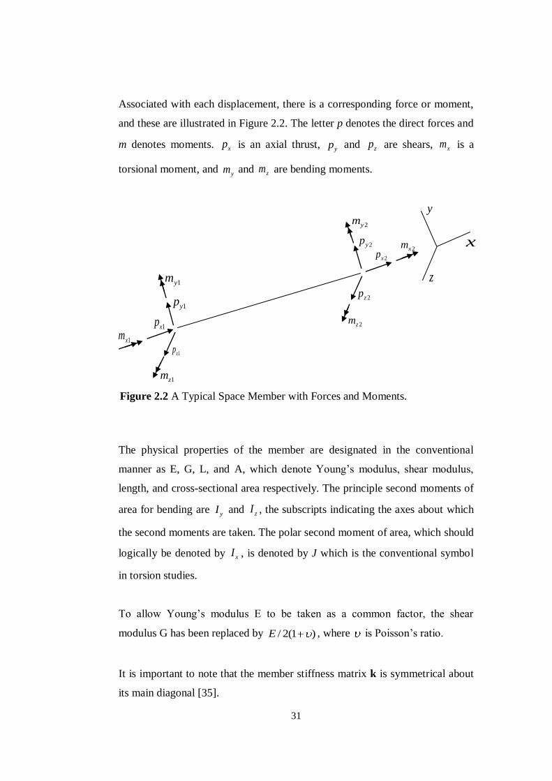
2.3 Stiffness Matrix of a Space Member
p = kd (2.3)
This is the member stiffness equation in which p and d are 12-term vectors of
member force and displacement respectively, and k is a 12x12 member
stiffness matrix for most general case of a prismatic member in space (shear
deformation is neglected), and with the implicit condition that the deformations
are so small as to leave the basic geometry unchanged.
If a member in space is taken into account, there is the possibility of three
linear displacements and three rotations at each of the member as shown in
Figure 2.1. The letter dx1 denotes linear displacements direction, and θx1
denotes rotations. The first suffix denotes the displacement direction, or the
axis about which a rotation takes place, while the second suffix denotes the
member end concerned. There are thus 12 possible displacement components
for the member, or 12 degrees of freedom.
1y
2z
2zd
31
x
y
z
1xm
1ym
2ym
2zm
1zm
2xm
2xp
1xp
1yp
2yp
2zp
1zp
Figure 2.2 A Typical Space Member with Forces and Moments.
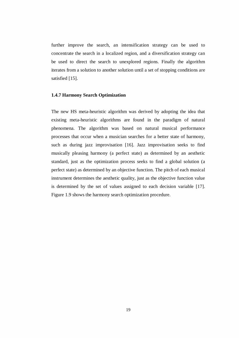
Associated with each displacement, there is a corresponding force or moment,
and these are illustrated in Figure 2.2. The letter p denotes the direct forces and
m denotes moments. xp is an axial thrust, yp and zp are shears, xm is a
torsional moment, and ym and zm are bending moments.
The physical properties of the member are designated in the conventional
manner as E, G, L, and A, which denote Young‟s modulus, shear modulus,
length, and cross-sectional area respectively. The principle second moments of
area for bending are yI and zI , the subscripts indicating the axes about which
the second moments are taken. The polar second moment of area, which should
logically be denoted by xI , is denoted by J which is the conventional symbol
in torsion studies.
To allow Young‟s modulus E to be taken as a common factor, the shear
modulus G has been replaced by / 2(1 )E , where is Poisson‟s ratio.
It is important to note that the member stiffness matrix k is symmetrical about
its main diagonal [35].
1
1
1
1
1
1
2
2
2
2
2
2
x
y
z
x
y
z
x
y
z
x
y
z
d
d
d
d
d
d
1
1
1
1
1
1
2
2
2
2
2
2
x
y
z
x
y
z
x
y
z
x
y
z
p
p
p
m
m
m
p
p
p
m
m
m
3 2 3 2
3 2 3 2
2 2
2 2
0 0 0 0 0 0 0 0 0 0
12 6 12 60 0 0 0 0 0 0 0
12 6 12 60 0 0 0 0 0 0 0
0 0 0 0 0 0 0 0 0 02 (1 ) 2 (1 )
6 4 6 20 0 0 0 0 0 0 0
6 4 6 20 0 0 0 0 0 0 0
0 0 0 0 0 0 0 0 0 0
120
z z z z
y y y y
y y y y
z z z z
EA EA
L L
EI EI EI EI
L L L L
EI EI EI EI
L L L L
J J
L L
EI EI EI EI
L L L L
EI EI EI EI
L L L L
EA EA
L L
E3 2 3 2
3 2 3 2
2 2
2 2
6 12 60 0 0 0 0 0 0
12 6 12 60 0 0 0 0 0 0 0
0 0 0 0 0 0 0 0 0 02 (1 ) 2 (1 )
6 2 6 40 0 0 0 0 0 0 0
6 2 6 40 0 0 0 0 0 0 0
z z z z
y y y y
y y y y
y z z z
I EI EI EI
L L L L
EI EI EI EI
L L L L
J J
L L
EI EI EI EI
L L L L
EI EI EI EI
L L L L
32
Figure 2.3 Stiffness matrix of a space member in local coordinate system.
33
Many structural members require less than the full matrix of 12 degrees of
freedom to express their deformations. Since a member in a space truss has pin
end connections, it cannot transmit any moment through its hinged ends.
Consequently, its deformation depends only on the linear displacements at each
end, which yields only three degrees of freedom at any joint. The stiffness
matrices in such cases may be obtained by selecting relevant terms from the
full matrix shown in Figure 2.3.
2.4 Derivation of a Nonlinear Stiffness Matrix Using Stability Functions
The axial forces in a member have a significant effect on its flexural bending
that cause nonlinearity in the behavior of structures. Therefore, it is of
importance to study this effect in the behavior of dome structures.
Structures which are subjected to both axial forces and bending moments are
called beam-column. Members carrying both axial force and bending moments
are exposed to an interaction between these effects. The lateral deflection of a
member causes additional bending moment when an axial force is applied. This
changes the flexural stiffness of the member. Similarly, the presence of
bending moments affects the axial stiffness of the member due to shortening of
the member caused by the bending deformations. If the deformations are small,
the interaction between bending and axial forces can be ignored. In such a case,
the force-deformation relationship for a beam-column is same as equation
(2.3). However, if the deformations are large, the stiffness matrix k is affected
by the interaction between bending and axial forces, and it is not linear
anymore [36]. The nonlinear stiffness matrix can be derived by using stability
functions.

34
2.4.1 Stability Functions
The stability functions are the modification factors from 1s to 9s . These
functions can be defined with respect to member length, cross-sectional
properties, axial force, and the end moments. The effect of axial force on
torsional stiffness and the effect of torsional moment on axial stiffness are
neglected [36].
where;
1s : stability function for the effect of flexure on axial stiffness,
2s : stability function for the effect of axial force on flexural stiffness
against rotation of near end about z-axis,
3s : stability function for the effect of axial force on flexural stiffness
against rotation of far end about z-axis,
4s : stability function for the effect of axial force on flexural stiffness
against rotation of near end about y-axis,
5s : stability function for the effect of axial force on flexural stiffness
against rotation of far end about y-axis,
6s : stability function for the effect of axial force on flexural stiffness
(about z-axis) against translation in y-direction,
7s : stability function for the effect of axial force on shear stiffness in y-
direction against translation in y-direction,

35
Y
X
ybF
X
P
Y
yaF
zbM
S
zaM
P
X P
P
Z
X
S
Z
yaM
zbF
ybM
zaF
8s : stability function for the effect of axial force on flexural stiffness
(about y-axis) against translation in z-direction,
9s : stability function for the effect of axial force on shear stiffness in z-
direction against translation in z-direction.
2.4.1.1 Effect of Flexure on Axial Stiffness
The axial stiffness of the beam in the absence of end moments is given by
EA/L, and the axial deformation due to axial loading P is given by PL/EA.
However, the end moments produce an additional axial deformation in the
beam. In order to include the effect of flexure on axial deformation, the axial
stiffness of the beam-column must be modified. For this purpose, the modified
axial stiffness can be illustrated as 1s (EA/L). An expression for 1s is derived as
follows [36].
(a)
(b)
Figure 2.4 Effect of Flexure on Axial Stiffness: (a) Bending in X-Y plane; (b)
Bending in X-Z plane

36
From Figure 2.4 (a) and (b);
2 2 2 2ds dx dy dz (2.4)
by rearranging this equation,
2 2 2
2 2 21
ds dy dz
dx dx dx (2.5)
Shortening due to bending can approximately be defined as,
bd ds dx (2.6)
dividing equation (2.6) by dx,
1bd ds
dx dx (2.7)
Neglecting higher order terms,
2 21
2
bd dy dz
dx dx dx (2.8)
Therefore, the shortening of the beam-column due to bending is,
0
L
bb
ddx
dx (2.9)
2 2
0
1
2
L
b
dy dzdx
dx dx (2.10)

37
Total shortening of the beam-column is expressed,
t shortening due to axial load ( a ) + shortening due to bending ( b )
2 2
0
1
2
L
t
PL dy dzdx
EA dx dx (2.11)
2 2
0
12
L
t
PL EA dy dzdx
EA PL dx dx (2.12)
1
t
P
EAs
L
(2.13)
and 1 2 2
0
1
12
Ls
EA dy dzdx
PL dx dx
(2.14)
The curvature 2
2
d y
dx can be defined from Figure (2.4) (a),
2
2
1( )za za zb
z
d y xM M M Py
dx EI L (2.15)
Let 2
z
P
EI (2.16)
Substituting equation (2.16) in equation (2.15) and rearranging the terms,

38
2 2 22
2 za zb za
d yy M M x M
dx PL P (2.17)
The solution for equation (2.17) is given by the summation of complementary
function and particular integral;
sin cos ( ) zaza zb
Mxy A x B x M M
PL P (2.18)
Substituting the boundary conditions y=0 at x=0 and x=L,
1cosec cos
and
za zb
za
A L M L MP
MB
P
(2.19)
The slope of beam in the X-Y plane is given by,
1cos sin za zb
dyA x B x M M
dx PL (2.20)
Similarly, the equation of the beam-column for bending in the X-Z plane is
sin sinya
ya yb
Mxz C x D x M M
PL P (2.21)
where 2
y
P
EI (2.22)
Substituting the boundary conditions z=0 at x=0 and x=L,

39
1cosec cos
and
ya yb
ya
C L M L MP
MD
P
(2.23)
The slope of the beam in the X-Z plane is given by,
1cos sin ya yb
dzC x D x M M
dx PL (2.24)
Now the integrals in equation (2.14) can be evaluated. The final result of the
integration is;
2
2 2 2
2
0
1[ cot cosec
2
L
za zb
dydx L M M L L L
dx P L
22 2 cosec 1 cot ]za zb za zbM M LM M L L L (2.25)
where; 2 2 2[ cot cosecz za zbH L M M L L L
2
2 2 cosec 1 cot ]za zb za zbM M LM M L L L
2
1
2zH
P L (2.26)
and
2
2 2 2
2
0
1[ cot cosec
2
L
ya yb
dzdx L M M L L L
dx P L
2
2 2 cosec 1 cot ]ya yb ya ybM M LM M L L L (2.27)

40
where; 2 2 2[ cot cosecy ya ybH L M M L L L
2
2 2 cosec 1 cot ]ya yb ya ybM M LM M L L L
2
1
2yH
P L (2.28)
Therefore, equation (2.14) becomes,
1
3 2
1
14 y z
sEA
P L H H
(2.29)
Note that; when end moments are absent, 1s becomes unity.
A similar approach can be used to derive an expression for 1s for a beam-
column with axial tensile force P. The final expression is as follows:
1
3 2 ' '
1
14 y z
sEA
P L H H
(2.30)
where; ' 2 2 2coth cosechy ya ybH L M M L L L
2
2 2 cosech 1 cothya yb ya ybM M LM M L L L (2.31)
and
' 2 2 2coth cosechz za zbH L M M L L L
22 2 cosech 1 cothza zb za zbM M LM M L L L (2.32)

41
2.4.1.2 Effect of Axial Force on Flexural Stiffness
2.4.1.2.1 Bending in X-Y Plane
From Figure 2.4 (a), the differential equation of the beam-column bending in
the X-Y plane is given by Equation (2.17) for which the solution is given by
equation (2.18). The constants A and B are obtained from Equation (2.19). The
end slopes of the beam-column are obtained by substituting x=0 and x=L in
equation (2.20);
0
1za za zb
x
dyA M M
dx PL (2.33)
1cos sinzb ya yb
x L
dyA L B L M M
dx PL (2.34)
Equations (2.33) and (2.34) can be rearranged and rewritten in matrix form as;
2 3
3 2
4 2
2 4
z z
za za
zb zbz z
EI EIs s
L LM
M EI EIs s
L L
(2.35)
when P is compressive, the 2s and 3s functions take the following form;
2
sin cos1
4 2 2cos sin
L L Ls L
L L L (2.36)
3
sin1
2 2 2cos sin
L Ls L
L L L (2.37)

42
For members subject to axial tensile force P and bending in the X-Y plane, P is
replaced by –P in equation (2.15). Solving the resulting differential equation,
equation (2.35) can again be obtained as;
2
cosh L sinh1
4 2 2cosh sinh
L Ls L
L L L (2.38)
3
sinh1
2 2 2cosh sin
L Ls L
L L L (2.39)
2.4.1.2.2 Bending in X-Z Plane
From Figure 2.4 (b), and following the same procedure previously mentioned,
the stability functions for bending in X-Z plane can be derived. The relationship
between end moments and end slopes is given by;
4 5
5 4
4 2
2 4
y y
ya ya
yb yby y
EI EIs s
L LM
M EI EIs s
L L
(2.40)
where;
4
sin cos1
4 2 2cos sin
L L Ls L
L L L for compressive P (2.41)
4
cosh sinh1
4 2 2cosh sinh
L L Ls L
L L L for tensile P (2.42)
and

43
zbM
zaM
P
P X
Y
yaF
ybF
y
L
5
sin1
2 2 2cos sin
L Ls L
L L L for compressive P (2.43)
5
sinh1
2 2 2cosh sinh
L Ls L
L L L for tensile P (2.44)
2.4.1.3 Effect of Axial Force on Stiffness Against Translation
If both of the ends of a beam-column are restrained against rotation, but one
end is translated trough a distance relative to the other, the flexural and
shear stiffnesses of the beam against this translation are affected by the axial
force P.
Figure 2.5 Effect of Axial Force on Stiffness Against Translation
2.4.1.3.1 Translation in X-Y Plane
From Figure 2.5, and using the slope-deflection equation;
2 3
4 2y yz zza
EI EIM s s
L L L L (2.45)

44
2 32
6 2 1
3 3
zy
EIs s
L (2.46)
6 2
6 zy
EIs
L (2.47)
where;
6 2 3
2 1
3 3s s s (2.48)
Substituting the values of 2s and 3s from equations (2.36) and (2.37) when the
axial force is compressive, and from equations (2.38) and (2.39) when the axial
force is tensile, the expressions for 6s can be obtained as;
When P is compressive;
2 2
6
1 (1 cos )
6 (2 2cos sin )
L Ls
L L L (2.49)
When P is tensile;
2 2
6
1 (cosh 1)
6 (2 2cosh sinh )
L Ls
L L L (2.50)
Once again from Figure 2.5,
ya
MF
L (2.51)

45
where;
za zb yM M M P (2.52)
and
2 3
4 2y yz zza
EI EIM s s
L L L L (2.53)
3 2
2 4y yz zzb
EI EIM s s
L L L L (2.54)
Thus,
2 33 3
8 4z zya y
EI EI PF s s
L L L (2.55)
If 2
z
P
EI is taken;
2 2
2 3 73 3
12 122 1
3 3 12
z zya
EI EILF s s s
L L (2.56)
where;
2 2
7 2 3
2 1
3 3 12
Ls s s (2.57)
Substituting for 2s and 3s from equations (2.36) and (2.37) when axial force is
compressive;

46
2 2 2 2
7
1 cos1
6 2 2cos sin 12
L L Ls
L L L (2.58)
When the axial force P is tensile, P is replaced by –P in equation (2.52) and
values of 2s and 3s are obtained from equations (2.38) and (2.39);
2 2 2 2
7
cosh 11
6 2 2cosh sinh 12
L L Ls
L L L (2.59)
2.4.1.3.2 Translation in X-Z Plane
Proceeding as in the previous section, 8s can be given;
8 4 5
2 1
3 3s s s (2.60)
Substituting the values of 4s and 5s from equations (2.41) and (2.43) when the
axial force is compressive, and from equations (2.42) and (2.44) when the axial
force is tensile, the expressions for 8s is shown as;
2 2
8
1 cos1
6 2 2cos sin
L Ls
L L L (2.61)
When P is tensile;
2 2
8
cosh 11
6 2 2cosh sinh
L Ls
L L L (2.62)
Proceeding as in the previous section, 9s can be derived;

47
2 2
9 4 5
2 1
3 3 12
Ls s s when the axial force P is compressive (2.63)
2 2
9 4 5
2 1
3 3 12
Ls s s when the axial force P is tensile (2.64)
Substituting the values of 4s and 5s from equations (2.41) and (2.43) when the
axial force is compressive, and from equations (2.42) and (2.44) when the axial
force is tensile, the expressions for 9s is shown as;
When P is compressive;
2 2 2
9
1 cos1
6 2 2cos sin 12
L L Ls
L L L (2.65)
When P is tensile;
2 2 2 2
9
cosh 11
6 2 2cosh sinh 12
L L Ls
L L L (2.66)
The nonlinear stiffness matrix using the stability functions 1s through 9s is
shown below in Figure 2.6.

48
Figure 2.6 Nonlinear stiffness matrix for three-dimensional beam-column element in local coordinate system.
1
1
1
1
1
1
2
2
2
2
2
2
x
y
z
x
y
z
x
y
z
x
y
z
p
p
p
m
m
m
p
p
p
m
m
m
1 1
7 6 7 63 2 3 2
9 8 9 83 2 3 2
8 4 8 52 2
6 2 6 32 2
0 0 0 0 0 0 0 0 0 0
12 6 12 60 0 0 0 0 0 0 0
12 6 12 60 0 0 0 0 0 0 0
0 0 0 0 0 0 0 0 0 0
6 4 6 20 0 0 0 0 0 0 0
6 4 6 20 0 0 0 0 0 0 0
z z z z
y y y y
y y y y
z z z
EA EAs s
L L
EI EI EI EIs s s s
L L L L
EI EI EI EIs s s s
L L L L
GJ GJ
L L
EI EI EI EIs s s s
L L L L
EI EI EIs s s s
L L L
1 1
7 6 7 63 2 3 2
9 8 9 83 2 3 2
8 5 8 42 2
6 3 62 2
0 0 0 0 0 0 0 0 0 0
12 6 12 60 0 0 0 0 0 0 0
12 6 12 60 0 0 0 0 0 0 0
0 0 0 0 0 0 0 0 0 0
6 2 6 40 0 0 0 0 0 0 0
6 2 60 0 0 0 0 0 0
z
z z z z
y y y y
y y y y
z z z
EI
L
EA EAs s
L L
EI EI EI EIs s s s
L L L L
EI EI EI EIs s s s
L L L L
GJ GJ
L L
EI EI EI EIs s s s
L L L L
EI EI EIs s s
L L L2
40 zEI
sL
1
1
1
1
1
1
2
2
2
2
2
2
x
y
z
x
y
z
x
y
z
x
y
z
d
d
d
d
d
d

49
2.5 Geometric Nonlinearity
A variety of classifications may be used to describe the deformational response
of structures; for example, small or large, elastic or inelastic, etc. In general,
deformations of structures under the external loads are small, and hence the
application of the equilibrium equations on the undeformed shape of the
structure does not introduce large errors. However, when structure consists of
slender members, the deformations become large and small deflection theory is
no longer valid. The equilibrium equations are required to be written in such
structures on the deformed shape of its elements. In other words, the deflected
shape of the structure should be taken into account. When this is considered in
the displacement computations, the relationship between the external loads and
displacements become nonlinear.
Geometric nonlinearity is required to be considered in the analysis of a
structure, if its deflections are large compared with its initial dimensions. In
structures with large displacements, although the material behaves linear
elastic, the response of the structure becomes nonlinear [19]. Under certain
types of loading, namely, even when small deformations are presumed,
nonlinear behavior can be predicted. Changes in stiffness and loads occur as
the structure deforms. When geometric nonlinearity occurs in a structure, the
effect of axial forces to member stiffness must be taken into account.
2.5.1 Construction of Overall Stiffness Matrix
After setting up the nonlinear member stiffness matrix in local coordinate
system displacement transformation matrix is conducted.
The equation (2.3) can be rewritten for a 3D truss member in local coordinates;
p=kd (2.67)

50
Now, the stiffness matrix in terms of local coordinates (k) must be converted to
stiffness matrix in terms of global coordinates (K). The transformation
equation of stiffness matrix from local to global coordinates is given below;
K = TT k T (2.68)
where;
K = global stiffness matrix,
k = local stiffness matrix,
T = transformation matrix (from local to global coordinates).
Although in theory the direction cosine matrices for each member of a structure
may be set up from the orientation of the members in terms of the structure
axes, in practice this can cause some difficulty. It is convenient, therefore, to
restate a rotation matrix R0 in terms of the projections of the members on the
structure axes. This can most easily be done by imagining the members as
initially lying in the x‟-direction with their y- and z-axes coinciding with y‟ and
z‟, and then moving by a series of three rotations to their final positions. The
rotations are i ) a rotation α about y-axis; ii ) a rotation β about the z-axis; and
iii ) a rotation γ about the x-axis. (Although there is a number of ways in which
a member might be moved from its initial to its final position, it is essential to
this derivation that the order indicated is preserved.)
Rotation α about y-axis : Figure 2.7 shows the rotation α of the member OA
to OA‟. It is a rotation in the xy plane. The rotation matrix Rα;
Rα =
cos 0 sin
0 1 0
sin 0 cos
(2.69)

51
Figure 2.7 Rotation α about y-axis
At this stage;
'
'
'
x x
y R y
z z
(2.70)
Rotation β about z-axis; Figure 2.8 shows the rotation β of the member from
position OA‟ to OA‟‟. It is rotation in the xy plane. The rotation matrix Rβ;
Rβ =
cos sin 0
sin cos 0
0 0 1
(2.71)
y
y'
x
x'
z'
z
A
A'
O
α
α

52
Figure 2.8 Rotation β about z-axis
The effect of this second rotation is obtained by premultiplying the result of
Equation (2.70) by Rβ.
At this stage ;
'
'
'
x x
y R R y
z z
(2.72)
Rotation γ about x-axis; Rotations α and β bring the member to its final
position, but its z-axis need not to be in the x‟z‟ plane. If, for instance, the x‟y‟
plane is a vertical plane, and the member is an I section with its web vertical
y y'
x
x'
z'
z
A'O
A''
A
B
C
D
ß
a
α
α
β
β

53
when first placed along the x‟-axis, then the web is still in a vertical plane after
rotations α and β. If the web is inclined to the vertical in the final position, then
a further rotation γ is required as shown in Figure 2.9.
Figure 2.9 Final rotation γ of the member about yz plane
The rotation matrix Rγ;
Rγ =
1 0 0
0 cos sin
0 sin cos
(2.73)
y'
z'
O
initial position of member
position of member after rotations α and β
final position of member
γ

54
The effect of this final rotation is obtained by premultiplying the result of
Equation (2.72) by Rγ. The final state is
'
'
'
x x
y R R R y
z z
(2.74)
Then; R0=RγRβRα
If the member OA is of length L, and its projections in its final position OA‟‟
on the x‟-,y‟-, and z‟-axes are Lx, Ly, and Lz respectively, then it can be seen
from Figure 2.8 that;
OC=Lx , OD=Ly=BA‟‟ , BC=-Lz , OB= 2 2 2 2( ) ( )y x zL L L L
Hence;
2 2
2 2
2 2
cos / / ( )
sin / ( )
cos ( ) /
sin /
x x z
z x z
x z
y
OC OB L L L
L L L
L L L
L L
(2.75)
Equation (2.75) gives the most general form of the rotation matrix.
2 2
02 2 2 2
2 2
2 2 2 2
/ / /
( cos sin ) ( cos sin )( ) cos
( ) ( )
( sin cos ) ( sin cos )( ) sin
( ) ( )
x y z
x y z y z xx z
x z x z
x y z y z xx z
x z x z
L L L L L L
L L LL L L LLL LR R R R
LL L L L L L
L L LL L L LLL L
LL L L L L L

55
So, that is to say, direct forces in structure axes are affected only by the direct
forces in member axes, and moments in structure axes are affected only by the
direct forces in member axes. The form of transformation matrix (T) is;
0
0
0
0 (12 12)
0 0 0
0 0 0
0 0 0
0 0 0x
R
RT
R
R
(2.76)
After developing the stiffness matrices for each member of the entire structure
in terms of local coordinates, these matrices can be assembled to form the
global stiffness matrix for the entire structure. Total stiffness at a coordinate is
the sum of the stiffnesses contributed to that coordinate by each element
attached to that coordinate.
The nonlinear response of a structure is obtained through successive linear
elastic analysis as shown in Figure 2.10. Initially the axial forces are presumed
to be zero. With zero values of axial forces, stability functions become
equal to 1. Linear elastic analysis of the structure is carried out and axial forces
in members are determined. With these values of axial forces the stability
functions are calculated and structural analysis is repeated. This process are
continued until the convergence is obtained in the axial force values of
members.

56
Figure 2.10 Nonlinear response of a structure obtained through successive
elastic linear analysis.
From Figure 2.10, an accurate set of joint displacements and member forces
become available for each load factor and nonlinear load-displacement diagram
of the structure can be plotted as shown in Figure 2.12 below.
START 1
5
2
7
3
4
6
8
9
Calculate the member end forces using P=kTX
Use the axial loads in the members and calculate their stability functions
Calculate the stability functions
using the new
member axial forces
Yes
No Is there convergence on
member axial forces?
INPUT DATA
Construct the overall stiffness matrix K
Solve the joint equilibrium equations L=KX for the joint displacements X (where; L=(L1,L2,…) applied forces, loads, and/or moments acting on structure.)
END
Axial Forces=0 Stability Functions (s1-s9)=1

57
Table 1 Y-displacement values of the joint 1 of the dome under different
external loads.
In order to show the difference between the displacement values obtained
through linear and nonlinear analysis, the dome structure shown in Figure 2.11
is considered.
Figure 2.11 A single layer lamella dome with 3 rings subjected to different
concentrated loads on its crown.
Loads (P)
(kN)
Y-displacements of the joint 1
of the dome (mm)
Number of
Nonlinear Iterations
From Nonlinear
Analysis
From Linear
Analysis
100 3 4.482 4.454
200 3 9.023 8.908
400 3 18.300 17.820
600 4 27.860 26.720
800 4 37.770 35.630
1000 4 48.140 44.540
1200 5 59.380 53.450
P
20 m
6.25 m

58
0 5 10 15 20 25 30 35 40 45 50 55 60 65 700
100
200
300
400
500
600
700
800
900
1000
1100
1200
1300
1400
Displacements (mm)
Lo
ad
s (k
N)
l inear analysis
nonlinear analysis
The dome is subjected to a concentrated load in Y-direction at its crown.
Y-displacements of the crown which is the first joint of the dome are calculated
by using linear and nonlinear analysis under different load levels. These are
shown in Table 1. The results obtained are plotted in Figure 2.12. The effect of
the geometrical nonlinearity on the values of Y-displacement of joint 1 is
clearly seen in this figure. At the load of 1200 kN, the nonlinear displacement
is 11.1% more than the linear displacement. It is clear that when the load is
increased, the axial forces increase in the members and their effect on the
flexural bending of the member become more emphasized. As a result
nonlinear displacement becomes larger.
Figure 2.12 Linear and nonlinear Y-displacements of joint 1 of the lamella
dome.
Figure 2.12 clearly reveals the fact that when the vertical loads become larger
in dome structures, the displacements become larger and inclusion of
geometric nonlinearity in the analysis of such structures becomes a necessity.

59
2.6 Elastic Critical Load Analysis
Elastic critical load analysis determines the load factor such that when the
loads are increased by this factor a structure loses its stability. The elastic
critical load analysis of structures involves iterative nonlinear analysis with
load increments. The flowchart shown in Figure 2.13 displays the steps of the
algorithm [35].
The stiffness matrix of a stable structure has the property of positive-
definiteness, and a test for this property is performed at each load level. At the
critical load the determinant of the stiffness matrix becomes zero which means
the stiffness matrix becomes singular. It is not easy to determine exactly at
what value of the load factor the determinant becomes zero. In practice when
the sign of the determinant of the stiffness matrix changes from positive to
negative, it is understood that the structure becomes unstable. The steps of the
algorithm are explained below;
1 ) The preparatory data should include the type of structure, such as space
frame, grillage, dome, etc., the number of the members, number of joints,
number of load cases and common material properties, such as Young‟s
modulus, shear modulus. The coordinates of each joint in the structure axes are
listed against the joint number. The members of structure with same sectional
properties are shown with the same group numbers. The support kind of the
members are given. The load case should be revealed in preliminary data. In
addition to this basic information, the preliminary data must include an initial
value for the load factor (LF), and the increment applied to load factor (INC).
2 ) N denotes the number of loading cycles and DET1, DET2, and DET3 are
the values of the determinant of the stiffness matrix. The axial forces in
members of the structure are not always known before the analysis begins, and
this chart assumes them all zero initially.
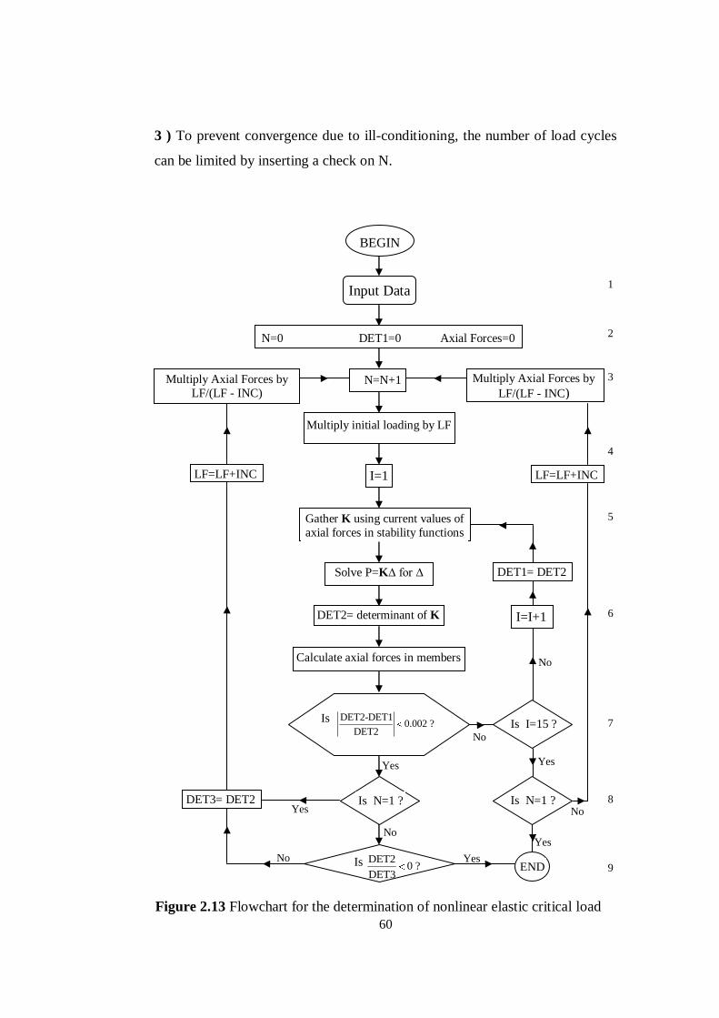
60
Figure 2.13 Flowchart for the determination of nonlinear elastic critical load
Analysis.
3 ) To prevent convergence due to ill-conditioning, the number of load cycles
can be limited by inserting a check on N.
Input Data
No
9
Yes
Yes
Gather K using current values of
axial forces in stability functions
Solve P=K∆ for ∆
DET2= determinant of K
Calculate axial forces in members
Is N=1 ? DET3= DET2
Is DET2-DET10.002 ?
DET2
I=I+1
DET1= DET2
END
Yes Yes
Yes
No
No
No
No
5
6
7
8
N=N+1 Multiply Axial Forces by
LF/(LF - INC)
Multiply Axial Forces by
LF/(LF - INC)
N=0 DET1=0 Axial Forces=0
I=1 LF=LF+INC LF=LF+INC
BEGIN
1
2
3
4
Multiply initial loading by LF
Is I=15 ?
Is N=1 ?
Is DET20 ?
DET3
61
4 ) A number of solutions which is counted by I are performed because initially
the axial forces at each load level are only known approximately.
5 ) The structure stiffness matrix K is set up by using stability functions as
shown in Figure 2.6.
6 ) When the terms of the stiffness matrix converge to a steady state at
consecutive cycles, the recurrent performed analysis at each load level should
be canceled. The determinant of the stiffness matrix DET2 is used as a suitable
control parameter as its value depends upon the stiffness matrix terms.
7 ) Once the proportional alteration in the determinant is less than %0.2, the
recurrent analysis is called off. This restriction value is completely random, but
it is reasonable in practice. The final determinant value is taken as the stiffness
matrix determinant stored in DET3 and this value is used for checking the
positive-definiteness.
8 ) When the loading approaches to the critical level, the stiffness matrix
becomes increasingly ill-conditioned and the determinant values become very
large. In such a case it is meaningless to keep repeated analysis going and it
should be terminated when I=15. If this termination occurs at first load level
(N=1), it means the loading is very near to critical level at the beginning. In
this case the analysis must be terminated and has to be renewed with a smaller
set of loads. In other respects, the load factor can be increased so that the axial
forces increase by the same ratio for examining further load levels.
9 ) As soon as the load level holds the satisfactory convergence, the value of
the determinant obtained is compared with that from the previous cycle. If no
sign change is observed then the load factor and axial forces are increased by
one step and a new load level is studied. If a sign change comes out (changing
from positive to negative), then the process is terminated.

62
As an example, if the dome in Figure 2.11 is considered once again under
different external loading, the determinant values of the stiffness matrix of the
dome for the last nonlinear analysis cycle which is the optimum design stored
as DET3 is shown in Table 2. It is obvious that dome can resist up to 1200 kN
external concentrated loading at its crown. If the loading exceeds this value, the
stiffness matrix of the dome changes its sign from positive to negative. This
means after critical loading value (1200 kN) the dome lost its stability and fail.
Table 2 Determinant values of the stiffness matrix of the dome.
Loads (P)
(kN)
Number of
nonlinear iterations
DET3
(stiffness matrix determinant)
100 3 0.397E+231
200 3 0.975E+230
400 3 0.350E+229
600 4 0.538E+227
800 4 0.263E+225
1000 4 0.234E+222
1200 5 0.100E+218
1400 3 -0.999E+194

63
CHAPTER 3
OPTIMUM DESIGN OF LAMELLA DOMES
3.1 Morphology of Lamella Domes
The morphology of the single layer lamella dome has a simple geometric form.
If the total number of rings and the height of the crown of the dome are known,
then it is very simple to get the whole topological information about the dome.
Utilizing the geometrical features of the lamella dome, the total number of
members and joints, and the member incidences can be established by the
knowledge about the total number of rings. One additional step to this, using
the geometric configuration and the height of crown of the dome, the exact
coordinates of all joint nodes can also be determined. Lamella domes with
varying crown heights and rings number, therefore, have dissimilar topology
from each other [33-34-37].
The form of commonly used single layer lamella dome is shown in Figure 3.1.
If the diameter of the dome D, the total number of rings nr, and the height of
the crown h are known, then all of the structural data about geometry of the
dome can be computed automatically. The distance between the rings in the
dome on the meridian line has to be equal. It can be easily seen from Figure 3.2
(b) that all the joints are located with equal distance from each other on the
same ring. The top joint at the crown is numbered as the first joint (joint
number 1). Every ring has 12 joints on itself. The first joint on the first ring
according to the positive z direction making an angle of 360o
/ 24 = 15o with
the radius drawn on the x axis is numbered as joint 2 and all of the first joints
of the other rings are placed as;

64
Figure 3.1 Lamella Dome.
(b) Plan
1 2
3
45
6
7
8
9
10 11
12
13
14
15
16
17
18
19
20
21
22
2324
25
26
27
2829
30
31
32
33
34 35
36
37
38
39
40
41
42
43
44
45
46
47
48
49
500 kN
(a) Elevation
20 m

65
D
Figure 3.2 Automated computation of joint coordinates in a lamella dome.
(b) Plan
1 2
3
45
6
7
8
9
10 11
12
13
14
15
16
17
18
19
20
21
22
23
24
25
26
28
38
40
41
X
Z
60°
75°
Xi
r=1 r=2 r=3 r=4
i
i
X
O
A B
43
2
Y
(a) Elevation
R
b b
y4
y3
y2
xi
yi
h
zi
15°
R-h
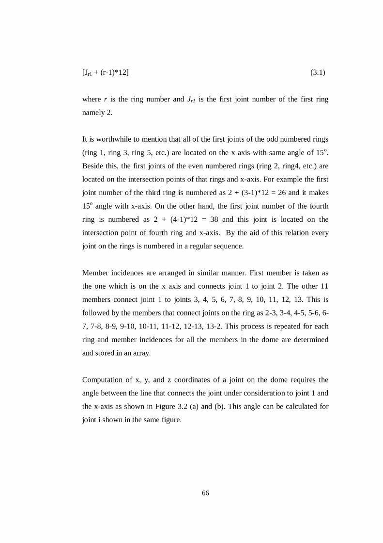
66
[Jr1 + (r-1)*12] (3.1)
where r is the ring number and Jr1 is the first joint number of the first ring
namely 2.
It is worthwhile to mention that all of the first joints of the odd numbered rings
(ring 1, ring 3, ring 5, etc.) are located on the x axis with same angle of 15o.
Beside this, the first joints of the even numbered rings (ring 2, ring4, etc.) are
located on the intersection points of that rings and x-axis. For example the first
joint number of the third ring is numbered as 2 + (3-1)*12 = 26 and it makes
15o angle with x-axis. On the other hand, the first joint number of the fourth
ring is numbered as 2 + (4-1)*12 = 38 and this joint is located on the
intersection point of fourth ring and x-axis. By the aid of this relation every
joint on the rings is numbered in a regular sequence.
Member incidences are arranged in similar manner. First member is taken as
the one which is on the x axis and connects joint 1 to joint 2. The other 11
members connect joint 1 to joints 3, 4, 5, 6, 7, 8, 9, 10, 11, 12, 13. This is
followed by the members that connect joints on the ring as 2-3, 3-4, 4-5, 5-6, 6-
7, 7-8, 8-9, 9-10, 10-11, 11-12, 12-13, 13-2. This process is repeated for each
ring and member incidences for all the members in the dome are determined
and stored in an array.
Computation of x, y, and z coordinates of a joint on the dome requires the
angle between the line that connects the joint under consideration to joint 1 and
the x-axis as shown in Figure 3.2 (a) and (b). This angle can be calculated for
joint i shown in the same figure.

67
For the odd numbered rings;
,1360*( )360
24 12
r
i
i j (3.2)
(2a)
For the even numbered rings;
,1360*( - )
12
r
i
i j (3.3)
(2b)
where i is shown in Figure 3.2 (b), r is the ring number that joint i is placed
on it and j is the first joint number on the ring number r which is on the x-axis.
For example, the angle between the radius that connects joint 1 to joint 16
located on a even numbered ring (ring 2) and the x-axis;
16
360*(16-14)60
12
o (3.4)
On the other hand, the angle between the radius that connects joint 1 to joint 28
located on a odd numbered ring (ring 3) and x-axis;
28
360 360*(28- 26)75
24 12
o
The ix and iz coordinates of joint i can be calculated as;
cos( )
sin( )
i i
i i
x ra
z ra (3.5)
(2c)

68
where r is the ring number that joint i is on it and a is the radius of ring r in x-z
plane.
If the distance between rings are equal to a, then a becomes D/(2nr). The iy
coordinate of joint i;
2 2
i iy R x R h (3.6) (2d)
where R is the radius of the semi-circle shown in Figure 3.2 (a) computed from
( D2
+ 4h2
) / (8h). By use of equations (3.5) and (3.6) for each joint, it is
possible to obtain the coordinates of the joints in the dome automatically.
3.2 Optimum Topology Design of Lamella Domes
Topological design of a lamella dome with a given base diameter necessitates
the finding out of the optimum number of rings and the height of the crown,
and the steel sections designations for each member group in the dome selected
from a standard steel sections table. These should be specified such that the
strength and serviceability requirements are satisfied according to code of
practice and the overall cost or only the material cost of the dome is minimum.

69
Figure 3.3 (a) Lamella Dome with Two Different Member Groups.
It is possible for the members of a dome to be made of the same section in
practice. However in some cases they can be grouped together to achieve the
minimum construction cost for the structure. The optimum topology design of
single layer lamella domes differs in formulation depending on the way
member grouping is decided in the dome [33-34]. If the members are chosen to
belong to the same group, dome becomes simple to design and member
grouping is independent of the number of rings. In another case, members
located in a meridian line can be one group and members on the rings are
another, total of two groups as shown in Figure 3.3 (a). In both cases number of
groups in the dome is not function of the number of rings and automatic
grouping of the members can be performed without the need of the total
1
11
1
1
1
1
111
1
1
1
1
11
1 1
11
1
1
1
1
1
1
1
111
11
1
1
1
1
11
1
1
1
1
1
1
1
1
111
1
1
1
1
1
1
1
1
1
11
1
1
1 1
1
1
1
1
1
1
1
1
1
1
111
1
1
1
1
1
1
1
2
22
2
2
2
2
2 2
2
2
2
2
2
2
2
2
2
2
2
2
2
2
2
2
22
2
2
2
2
2 2
2
2
2
22
2
2
2
2
22
2
2
2
2

70
number of rings in the dome. However, it is also possible that the members of
the dome can be grouped such that the members between each ring are to be
assigned one group and the members on each ring are another group as shown
in Figure 3.3 (b) [34-37]. In this case, the members between the crown and the
first ring are assigned as group 1, the members on the first ring are assigned as
group 2, the members between rings 1 and 2 are assigned as group 3, and the
group number of members on the ring 2 is assigned as group 4 and so on.
Under this circumstance, grouping of the members depend upon the total
number of rings which is one of the design variables of the problem. Hence the
total number of groups in the dome becomes twice the total number of rings in
the design problem. For example, if a dome with three rings is considered, the
total number of design variables becomes 7, six of which are the sectional
designation to be selected for each group and the last one is the height of the
dome. In the case of five rings in the dome the total number of design variables
is 11, ten of which represents the sectional designations to be assigned for each
group and the last one gives the height of the crown in the dome.

71
Figure 3.3 (b) Lamella Dome with Eight Different Member Groups.
3.3 Mathematical Model of Optimum Design Problem of Lamella Domes
According to LRFD-AISC
In three dimensional modeling of lamella domes, joints are considered to be
rigidly connected in order to represent real behavior of these domes. As a result
of such modeling, all members of the lamella dome are exposed to both axial
forces and bending moments. Consequently, axial stiffness of the members of
lamella dome are influenced by the bending moments directly because of
members‟ slenderness, which requires the consideration of the geometric
nonlinearity in the analysis of these structures.
1
11
1
1
1
1
111
1
1
3
22
2
2
2
2
22
2
2
2
2
3 33
3
3
3
3
3
3
3
33
333
3
3
3
3
3
3
3
3
4
4
4
4
4 4
4
4
4
4
44
5
5
55 5
5
5
5
5
5
5
5
5
5
555
5
5
5
5
5
5
5
6
6
6
6
6
6
6
6
6
6
6
6
7
7
7
7
7 7
7
7
7
7
7
7
7
7
7
777
7
7
7
7
7
7
8
8
8
8 8
8
8
8
8
88
8

72
The design of lamella domes requires the selection of steel sections for its
members from a standard steel pipe section tables such that the dome satisfies
the serviceability and strength requirements specified by the code of practice
while the economy is observed in the overall or material cost of the dome.
When the design constraints are implemented from LRFD-AISC [38-39] in the
formulation of the design problem the following mathematical programming
problem is obtained.
1 1
minisng
i j
i j
W m l (3.7)
Subject to;
k ku , 1,2,.....,k p (3.8)
For 0.2u
n
P
P;
81
9
uyu ux
n b nx b ny
MP M
P M M (3.9)
For 0.2u
n
P
P;
12
uyu ux
n b nx b ny
MP M
P M M (3.10)
v nr urV V , 1,2,.....,r nm (3.11)

73
where im in equation (3.7) gives the unit weight of a lamella dome member
belonging to group i selected from steel pipe section list of LRFD-AISC, is is
the total number of members in group i, and ng is the total number of groups
in the dome system. jl is the length of member j . kδ in equation (3.8) is the
displacement of joint k and ku δ is its upper bound. The joint displacements are
computed by carrying out elastic-critical load analysis for lamella dome
system.
Equations (3.9) and (3.10) represent the strength requirements for a member
subjected to both bending and axial force according to LRFD. In these
inequalities Øb is the resistance factor for flexure given as 0.9, is the
resistance factor for compression given as 0.85, Mux is the required flexural
strength relating to strong axis (x) bending, Muy is the required flexural strength
related with the weak axis (y) bending, Mnx and Mny are the nominal flexural
strength related with strong axis (x) bending and weak axis (y) bending
respectively. Pu is the required compressive strength, and Pn is the nominal
compressive strength which is computed from;
n g crP A F (3.12)
Subjected to;
For 1.5c
2
(0.658 )c
cr yF F (3.13)
(1g)
74
For 1.5c
2
0.877cr y
c
F F (3.14)
(1h)
where in equation (3.12) Ag is the gross area of a lamella dome member, and
Fcr is found from equation (3.13) or (3.14) in which Fy is the specified yield
stress taken as 250 MPa and c is obtained from;
y
c
FKl
r E (3.15)
where K is the effective length factor taken as 1, l is the length of a dome
member, r is governing radius of gyration about the axis of buckling, and E is
the modulus of elasticity.
Equation (3.11) represents the shear strength requirement in load and resistance
factor design according to LRFD. In this inequality v represents the resistance
factor for shear given as 0.9, Vnr is the nominal strength in shear and Vur is the
factored service load shear for member r.
The programming problem described with equations (3.7) to (3.11) is discrete
programming problem due to the fact that pipe sections for the groups of the
dome are to be selected from the available steel pipe section lists. Harmony
search method is used to obtain the solution of this problem. It should be
pointed out that the nominal flexural strength and the axial strength of the
dome members are calculated by carrying out elastic critical load factor
analysis of the dome as explained in Chapter 2.

75
CHAPTER 4
HARMONY SEARCH METHOD BASED OPTIMUM
DESIGN ALGORITHM
4.1 General Concept of Harmony Search Algorithm
Numerical methods which have the shortcomings, such as using gradient
information and motivated improving the solution in the neighborhood of a
starting point, have compelled researchers to use meta-heuristic algorithms
counterfeiting a natural phenomena such as genetic algorithms (GAs), tabu
search (TS), simulated annealing (SA), evolutionary strategies (ES), etc.
Among these methods, a new meta-heuristic algorithm is called harmony
search (HS) method is developed by Geem [16]. This numerical technique
simulates the musical performance process that comes about once a musician is
looking for a better state of harmony. Jazz improvisation seeks to find
musically pleasing harmony similar to the optimum design process which seeks
to find the optimum solution. The HS algorithm demands fewer mathematical
requirements and does not need initial values for decision variables and the
derivative information of the objective function and constraints when
compared to mathematical programming methods mentioned above. Thereby,
the harmony search method enables easy programming among the
combinatorial optimization algorithms.

76
The harmony search method consists of five basic steps [40];
Step 1. Initialize the problem and algorithm parameters.
Step 2. Initialize the harmony memory.
Step 3. Improvise a new harmony.
Step 4. Update the harmony memory.
Step 5. Check the stopping criteria.
The detailed descriptions of these steps can be useful to comprehend the HS
method clearly.
Step 1. Harmony search parameters are initialized.
A possible value range for each design variable of the optimum design problem
is specified as:
Minimize f(x), xЄX (4.1)
Subject to g(x) ≥ 0 and h(x) = 0 (4.2)
where; f(x) is the objective function and g(x) is the inequality constraint
function; h(x) is the equality constraint function. x is the set of each decision
variable, xi, and X is the set of the possible range of values for each decision
variable, that is Lxi ≤ Xi ≤ Uxi, where Lxi and Uxi are the lower and upper bounds
for each decision variable.

77
A pool is constructed by collecting these values together from which the
algorithm selects values for the design variables. Furthermore the number of
solution vectors in harmony memory (HMS) that is the size of the harmony
memory matrix, harmony considering rate (HMCR), pitch adjusting rate (PAR)
and the maximum number of searches are also specified in this step.
Step 2. Harmony memory matrix (HM) is initialized.
Harmony memory matrix is initialized. Each row of harmony memory matrix
contains the values of design variables which are randomly selected feasible
solutions from the design pool for that particular design variable. Hence, this
matrix has n columns where n is the total number of design variables, and
HMS rows are selected in the first step. HMS is similar to the total number of
individuals in the population matrix of the genetic algorithm. The harmony
memory matrix has the following form:
[H] =
hmsnhmsnhmshms
hmsnhmsnhmshms
nn
nn
xxxx
xxxx
xxxx
xxxx
,,1,2,1
1,1,11,21,1
2,2,12,22,1
1,1,11,21,1
....
....
............
............
....
....
(4.3)
jix , is the value of the ith
design variable in the jth
randomly selected feasible
solution. These candidate designs are sorted such that the objective function
value corresponding to the first solution vector is the minimum. In other words,
the feasible solutions in the harmony memory matrix are sorted in descending
order according to their objective function values. It is worthwhile to mention
that only the feasible designs which satisfy the constraints are inserted into
harmony memory matrix. Those designs having a small infeasibility are also
included in the harmony memory matrix with a penalty on their objective

78
function. A detailed flowchart for the improvisation of a new harmony memory
matrix is given in Figure 4.1.
Step 3. New harmony memory matrix is improvised.
In generating a new harmony matrix the new value of the ith design variable
can be chosen from any discrete value within the range of ith
column of the
harmony memory matrix with the probability of HMCR which varies between
0 and 1. In other words, the new value of xi can be one of the discrete values of
the vector T
hmsiii xxx ,2,1, ..,,........., with the probability of HMCR . The same
is applied to all other design variables. In the random selection, the new value
of the ith
design variable can also be chosen randomly from the entire pool with
the probability of HMCR1 . That is
,1 ,2 ,
1 2
, ,...........
, ,..........., (1 )
T
i i i i hms
new
iT
i ns
x x x x with probability HMCR
x
x x x x with probability HMCR
(4.4)
where ns is the total number of values for the design variables in the pool. If
the new value of the design variable is selected among those of harmony
memory matrix, this value is then checked whether it should be pitch-adjusted.
This operation uses pitch adjustment parameter PAR that sets the rate of
adjustment for the pitch chosen from the harmony memory matrix as follows:
PARofyprobabilitwithNo
PARofyprobabilitwithYesadjustedpitchbetoxIs new
i1
? (4.5)
Supposing that the new pitch-adjustment decision for newix came out to be yes
from the test and if the value selected for newix from the harmony memory is
the kth
element in the general discrete set, then the neighboring value k+1 or
79
k-1 is taken for new newix . This operation prevents stagnation and improves
the harmony memory for diversity with a greater change of reaching the global
optimum.
Constraint handling: Once the new harmony vector newix is obtained using
the above-mentioned rules, it is then checked whether it violates problem
constraints. If the new harmony vector is severely infeasible, it is discarded. If
it is slightly infeasible, there are two ways to follow. One is to include them in
the harmony memory matrix by imposing a penalty on their objective function
value. In this way the violated harmony vector which may be infeasible slightly
in one or more constraints, is used as a base in the pitch adjustment operation
to provide a new harmony vector that may be feasible. The other way is to use
larger error values such as 0.08 initially for the acceptability of the new design
vectors and reduce this value gradually during the design cycles and use finally
an error value of 0.001 towards the end of the iterations. This adaptive error
strategy is found quite effective in handling the design constraints in large
design problems.
Step 4. Harmony Memory matrix is updated.
After selecting the new values for each design variable the objective function
value is calculated for the new harmony vector. If this value is better than the
worst harmony vector in the harmony matrix, it is then included in the matrix
while the worst one is taken out of the matrix. The harmony memory matrix is
then sorted in descending order by the objective function value.
Step 5. Steps 3 and 4 are repeated until the termination criterion which is the
pre- selected maximum number of cycles is reached. This number is selected
large enough such that within this number of design cycles no further
improvement is observed in the objective function.

80
.
Figure 4.1 Improvisation of a new harmony memory vector.
ran ≤ 0.5
Yes
No
Start
Number of mxi
Stop
ran < HMCR
i > m
D3 = int(ran*HMS)+1
D4 = HM(D3, i )
NCHV( i )=D4
D3 = int(ran*NS)+1
D4 = HM(D3, i )
NCHV( i )=D4
ran < PAR
D3 = D3+1
NCHV( i ) = HM(D3,i)
D3 = D3-1
NCHV( i ) =HM(D3,i)
ix : Continuous variables ( mi ,,2,1 )
HMCR: Harmony memory considering rate
NS: The total number of values for the
design variables in the discrete set (pool)
PAR: Pitch adjustment rate
HMS: Harmony memory size
HM(*,*):Harmony memory matrix
ran: Random numbers in the range 0.0 ~ 1.0
NCHV: A new harmony vector
Yes
Yes
No
Yes
No
No
81
4.2 A Harmony Search Algorithm Based Optimum Design Method For
Single Layer Lamella Domes
Optimum topological design problem of single layer lamella domes under a
given loading case, mathematical formulation of which is shown in Equations
3.7-3.11, is solved by using harmony search method. The steps of the design
algorithm developed are given as follows;
1. Prepare the discrete sets. In this step, discrete design pools are prepared for
the design variables since there are three different types of design variables,
three different design pools are prepared; one for each. There are a set of steel
sections selected from the available pipe section lists, a set of discrete height
values and a set of total ring numbers. The steel pipe sections, height values,
and number of rings are sorted in ascending order according to weight per
meter, minimum height to maximum height, and minimum ring number to
maximum ring number, respectively. The design pool for the total number of
rings for the dome contains 4 values that are 3, 4, 5 and 6. For the height of the
crown a list is prepared starting from 1 m to 8.75 m with the increment of
0.25 m, resulting 32 discrete values as shown in Table 4.1. The size design
variables (members‟ ready sections) are selected from 37 steel pipe sections
given in LRFD-AISC [38] as listed in Table 4.2. The sectional designations
selected vary from PIPST13 to PIPDEST203 where abbreviations ST, EST,
and DEST stands for standard weight, extra strong, and double-extra strong
respectively.
2. Select the values of harmony parameters. The harmony memory size
HMS, the harmony memory considering rate HMCR and the pitch adjustment
rate PAR are selected. These parameters are decided after carrying out several
trials.

82
3. Generate a harmony memory matrix. Select randomly total number of
rings, crown height and sequence number of a steel pipe section from the
discrete list for each group in the dome. The sequence numbers of steel pipe
sections, height values, and total number of rings varying between 1 to total
number of pipe sections, heights, and total number of ring are included in the
design pool. These sequence numbers are treated as design variable. For
example, if there are 37 steel pipe sections, 32 height values, and 4 ring
numbers in the design pool and 6 member groups in the truss dome to be
designed then the Harmony Search algorithm selects randomly integer numbers
which vary from 1 to 37 for steel pipe sections, 1 to 32 for height values, and 1
to 4 for ring number for each member group. Once the selection is carried out
for each member group, the cross sectional properties of each steel pipe section
become available from the design pool. The structure is then analyzed under
the external loads with these sections to find out whether its response is within
the limitations imposed by the design code.
Table 4.1 Discrete Set of Height Values.
Sequence Number Height (m) Sequence Number Height (m)
1 1.00 17 5.00
2 1.25 18 5.25
3 1.50 19 5.50
4 1.75 20 5.75
5 2.00 21 6.00
6 2.25 22 6.25
7 2.50 23 6.50
8 2.75 24 6.75
9 3.00 25 7.00
10 3.25 26 7.25
11 3.50 27 7.50
12 3.75 28 7.75
13 4.00 29 8.00
14 4.25 30 8.25
15 4.50 31 8.50
16 4.75 32 8.75

83
Table 4.2 Dimensions and Properties of Steel Pipe Sections.
1 2 3 4 5 6 7 8 9 10 11
1 PIPST13 21,3 2,77 160 0,00704 0,661 6,63 14,1 0,953 0,0125
2 PIPEST13 21,3 3,73 205 0,00827 0,777 6,35 16,5 1,16 0,0159
3 PIPST19 26,7 2,87 217 0,0156 1,17 8,48 31,2 1,65 0,0165
4 PIPEST19 26,7 3,91 282 0,0188 1,41 8,16 37,6 2,06 0,0215
5 PIPST25 33,4 3,38 320 0,0365 2,19 10,7 73 3,07 0,0245
6 PIPEST25 33,4 4,55 412 0,044 2,63 10,3 87,9 3,82 0,0317
7 PIPST32 42,2 3,56 431 0,0812 3,85 13,7 162 5,32 0,0332
8 PIPST38 48,3 3,68 518 0,13 5,38 15,8 260 7,38 0,0397
9 PIPEST32 42,2 4,85 569 0,101 4,79 13,3 202 6,8 0,0439
10 PIPEST38 48,3 5,08 692 0,164 6,79 15,4 327 9,56 0,0531
11 PIPST51 60,3 3,91 691 0,276 9,15 20 552 12,4 0,0534
12 PIPEST51 60,3 5,54 947 0,359 11,9 19,5 718 16,6 0,0734
13 PIPST64 73 5,16 1100 0,635 17,4 24 1270 23,8 0,0846
14 PIPST76 88,9 5,49 1440 1,26 28,3 29,6 2520 38,3 0,111
15 PIPEST64 73 7,01 1450 0,799 21,9 23,5 1600 30,6 0,112
16 PIPDEST51 60,3 11,1 1710 0,544 18 17,8 1090 27,3 0,132
17 PIPST89 102 5,74 1800 2,08 40,8 34 4160 55 0,133
18 PIPEST76 88,9 7,62 1940 1,62 36,4 28,9 3240 50,4 0,15
19 PIPST102 114 6,02 2040 2,98 52,3 38,2 5950 70,1 0,158
20 PIPEST89 102 8,08 2440 2,7 52,9 33,3 5400 73,1 0,183
21 PIPDEST64 73 14 2590 1,19 32,6 21,4 2390 49,6 0,2
22 PIPST127 141 6,55 2750 6,23 88,4 47,6 12500 118 0,214
23 PIPEST102 114 8,56 2790 3,91 68,6 37,4 7820 93,9 0,219
24 PIPDEST76 88,9 15,2 3530 2,5 56,2 26,6 4990 83,9 0,271
25 PIPST152 168 7,11 3540 11,5 137 57 23000 182 0,277
26 PIPEST127 141 9,53 3920 8,53 121 46,6 17100 165 0,304
27 PIPDEST102 114 17,1 5170 6,27 110 34,8 12500 161 0,402
28 PIPST203 219 8,18 5300 29,6 270 74,7 59100 356 0,417
29 PIPEST152 168 11 5430 16,8 200 55,6 33600 272 0,418
30 PIPDEST127 141 19,1 7280 13,9 197 43,7 27800 285 0,564
31 PIPST254 273 9,27 7460 65,1 477 93,4 130000 628 0,591
32 PIPEST203 219 12,7 8110 43,4 396 73,2 86800 534 0,634
33 PIPST305 324 9,53 9390 116 716 111 232000 940 0,724
34 PIPDEST152 168 21,9 10100 27,5 327 52,2 55000 473 0,777
35 PIPEST254 273 12,7 10200 87 637 92,4 174000 849 0,8
36 PIPEST305 324 12,7 12700 154 951 110 308000 1260 0,956
37 PIPDEST203 203 22,2 13600 66,9 611 70,1 134000 857 1,06
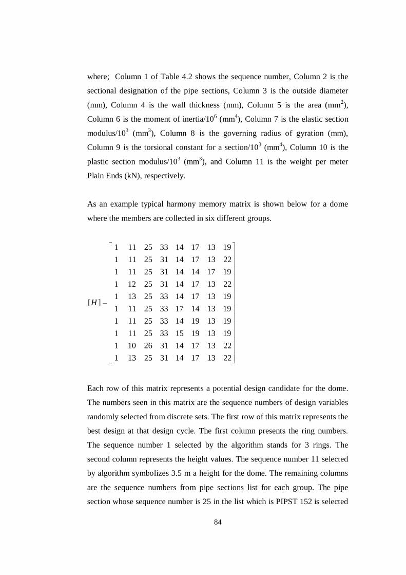
84
where; Column 1 of Table 4.2 shows the sequence number, Column 2 is the
sectional designation of the pipe sections, Column 3 is the outside diameter
(mm), Column 4 is the wall thickness (mm), Column 5 is the area (mm2),
Column 6 is the moment of inertia/106 (mm
4), Column 7 is the elastic section
modulus/103 (mm
3), Column 8 is the governing radius of gyration (mm),
Column 9 is the torsional constant for a section/103 (mm
4), Column 10 is the
plastic section modulus/103 (mm
3), and Column 11 is the weight per meter
Plain Ends (kN), respectively.
As an example typical harmony memory matrix is shown below for a dome
where the members are collected in six different groups.
1 11 25 33 14 17 13 19
1 11 25 31 14 17 13 22
1 11 25 31 14 14 17 19
1 12 25 31 14 17 13 22
1 13 25 33 14 17 13 19[ ]
1 11 25 33 17 14 13 19
1 11 25 33 14 19 13 19
1 11 25 33 15 19 13 19
1 10 26 31 14 17 13 22
1 13 25 31 14 17 13 22
H
Each row of this matrix represents a potential design candidate for the dome.
The numbers seen in this matrix are the sequence numbers of design variables
randomly selected from discrete sets. The first row of this matrix represents the
best design at that design cycle. The first column presents the ring numbers.
The sequence number 1 selected by the algorithm stands for 3 rings. The
second column represents the height values. The sequence number 11 selected
by algorithm symbolizes 3.5 m a height for the dome. The remaining columns
are the sequence numbers from pipe sections list for each group. The pipe
section whose sequence number is 25 in the list which is PIPST 152 is selected

85
for member group 1. Sequence number 33 corresponds to PIPST 305 which is
the pipe section adopted for group 2. The rest of the sections are given in
columns 5, 6, 7, and 8.
4. Generate the geometrical data such as member incidences and joint
coordinates, automatically using the values selected for the total number of
rings and crown height as explained in Chapter 3.
5. Carry out the nonlinear elastic critical load analysis of the steel dome with
the tubular sections selected for member groups until the ultimate load factor is
reached and check whether there is a loss of stability at any stage of this
nonlinear analysis as explained in Chapter 2. If the loss of stability occurs then
this selected design vector is taken out from harmony memory matrix and
replaced by a new design vector that is selected randomly again. This
replacement process is repeated until a design vector is determined that does
not have instability problem. This vector is then checked whether or not it
satisfies the design constraints. If it does not satisfy it is once more discarded.
However, if it is slightly infeasible it is considered for the harmony memory
matrix.
6. Check whether the new design vector selected should be pitch-adjusted as
explained in step 3 of the harmony search method.
7. Calculate the objective function value for the newly selected design vector.
If this value is better than the worst harmony vector in the harmony matrix, it is
then included in the matrix while the worst one is taken out of the matrix. The
harmony memory matrix is then sorted in descending order by the objective
function value. If the previous example is considered once more, the harmony
memory matrix includes the sequence numbers of design variables and the
weight (kg) which is the objective function of the dome (Table 4.3).

86
Table 4.3 A harmony set of a designed dome.
When the newly selected design vector, which is the 3rd
row, is better than the
worst harmony vector, the worst one is discarded from matrix and the new one
is added as seen in Table 4.4.
Table 4.4 New harmony set of a designed dome.
8. Repeat steps 2 and 6 until the pre-selected maximum number of iterations
is reached. The maximum number of iterations is selected large enough such
that within this number of design cycles no further improvement is observed in
the objective function.
The general flow diagram of the optimum topological design of single layer
lamella domes, based upon Harmony Search Method, can be described as in
following chart;
1 11 25 33 14 17 13 19 6348.59
1 11 25 31 14 17 13 22 6402.63
[ ] 1 11 25 31 14 14 17 19 6448.47
1 12 25 31 14 17 13 22 6449.17
1 13 25 33 14 17 13 19 6450.40
H
1 11 25 33 14 17 13 19 6348.59
1 11 25 31 14 17 13 22 6402.63
[ ] 1 12 25 31 14 17 13 22 6449.17
1 13 25 33 14 17 13 19 6450.40
1 11 25 33 17 14 13 19 6457.29
H

87
Figure 4.2 Flowchart of Harmony Search method based optimum design of
algorithm.
OPTIMIZED WEIGHT
IF IT IS ACCEPTABLE DESIGN INSERT IT
INTO THE HARMONY MEMORY MATRIX
Yes
No
INITIALIZE HARMONY SEARCH ANALYSIS
INPUT DATA
SELECT THE HARMONY SEARCH PARAMETERS
GENERATE GEOMETRICAL DATA
(Member incidences and joint coordinates)
END
CONSTRUCT THE MEMBER GROUPS
PERFORM ELASTIC CRITICAL LOAD ANALYSIS
CALCULATE THE STRUCTURAL WEIGHT OF THE DOME
Is maximum number of iterations reached?
PRINT RESULT OF OPTIMIZATION
IMPLEMENT THE DESIGN PROCEDURE
ACCORDING TO LRFD-AISC AND CHECK
WHETHER DESIGN CONSTRAINTS ARE STASFIED

88
CHAPTER 5
DESIGN EXAMPLES
The design algorithm presented is used to determine the optimum number of
rings, the crown height and the circular steel hollow section designations for
the single layer lamella dome shown in Figure 3.1. The preparation of the
design pool, for the steel pipe sections, the height of the crown and the total
number of rings, is explained in detail in the previous chapter. The modulus of
elasticity for the steel is taken as 205 kN/mm2 and the shear modulus is taken
as 81 kN/mm2. The diameter of the dome is taken as 20 m. The limitations
imposed on the joint displacements are given in Table 5.1.
Table 5.1 Displacement restrictions of the single layer lamella dome.
Harmony memory matrix size is initially taken as 20. However, the same
example is designed several times using different harmony memory matrix size
which was changed from 20 to 50. In the mean time harmony memory
considering rate (HMCR) and pitch-adjusting rate (PAR) are varied between
0.60 to 0.90 and 0.20 to 0.45 respectively in order to determine the most
Joint number
Displacement restrictions (mm)
X-direction Y-direction Z-direction
1 - - 28
2 33 33 28
3 33 33 28

89
appropriate values for the design problem under consideration. Table 5.2 shows
the effect of different values of harmony search algorithm parameters on the
optimum design. Different set of values yields different minimum weights.
Among these the lightest dome is selected which is the fourth one in the table.
Table 5.2 The effect of Harmony Search algorithm parameters.
Analysis HMS HMCR PAR Weight (kg) Height (m)
1 50 0.80 0.30 4214.9 3.75
2 30 0.90 0.30 4066.8 5
3 20 0.90 0.45 4038.8 5.75
4 50 0.85 0.40 4034.2 6.25
It is apparent from Table 5.2 that the selection of the above parameters is
problem dependent. The total number of iterations is taken as 20000 in each
design case. This number is determined after carrying out several designs with
a larger number of searches. It is noticed that the result obtained within the
20000 searches remains the same even if the search continues up to 50000 for a
better design. The design obtained in the last search is considered to be the
optimum solution. The member grouping is decided such that the total number
of groups in the dome becomes twice the total number of rings in the design
problem.
The dome is considered to be subjected to three loading case as follows;
1. P (5.1)
2. D + P (5.2)
3. D + P + W (5.3)

90
where; P is the equipment load acting on crown of the dome, D is the dead
load, and W is the wind load.
5.1 CASE 1 (P)
In this case dome is considered to be subjected to equipment loading of 500kN
at its crown as shown in Figure 3.1. The optimum sectional designations for
each group and the height obtained for the dome with different number of rings
are given in Table 5.3. It is noticed in all these cases that the strength
limitations are dominant in the design problem. In the optimum domes while
the strength ratios were equal to 1 or very close to 1, the restricted
displacements are much less than their upper bounds. Furthermore, it is clear
that the lightest dome among the four optimum geometries is the one which has
the least number of rings. It is apparent that the dome with a greater number of
rings has more members which naturally yield a heavier structure. Hence the
optimum number of rings for the lamella dome is three. All joints on the last
ring are considered to be pin support for this case. The optimum dome obtained
is shown in Figures 5.1 and 5.2.
Table 5.3 Optimum design for the single layer lamella dome for load case 1.
Group Number
Optimum Section Designations
3 rings 4 rings 5 rings 1 PIPST 127 PIPST 152 PIPST 203
2 PIPEST 89 PIPEST 89 PIPST 19
3 PIPST 64 PIPST 64 PIPST 64
4 PIPST 76 PIPST 76 PIPST 102
5 PIPST 64 PIPST 64 PIPST 64
6 PIPST 13 PIPST 76 PIPST 76
7 N.A PIPST 64 PIPST 64
8 N.A PIPST 13 PIPST 76
9 N.A N.A PIPST 64
10 N.A N.A PIPST 13
Optimum Height (m) 6.25 5.25 3.25
Max.Displacement (mm) 2.38 4.77 25.16
Max. Strength Ratio 0.98 1.00 1.00 Weight (kg) 4034.2 4502.1 4873.1

91
Figure 5.1 3D view of optimum single layer lamella dome.
Figure 5.2 Side view of optimum single layer lamella dome.
20 m
6.25 m 5.49 m
3.30 m
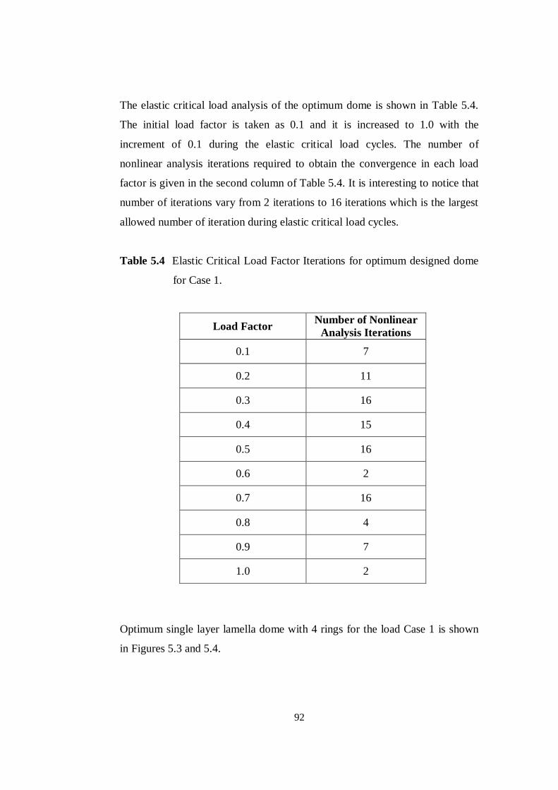
92
The elastic critical load analysis of the optimum dome is shown in Table 5.4.
The initial load factor is taken as 0.1 and it is increased to 1.0 with the
increment of 0.1 during the elastic critical load cycles. The number of
nonlinear analysis iterations required to obtain the convergence in each load
factor is given in the second column of Table 5.4. It is interesting to notice that
number of iterations vary from 2 iterations to 16 iterations which is the largest
allowed number of iteration during elastic critical load cycles.
Table 5.4 Elastic Critical Load Factor Iterations for optimum designed dome
for Case 1.
Load Factor Number of Nonlinear
Analysis Iterations
0.1 7
0.2 11
0.3 16
0.4 15
0.5 16
0.6 2
0.7 16
0.8 4
0.9 7
1.0 2
Optimum single layer lamella dome with 4 rings for the load Case 1 is shown
in Figures 5.3 and 5.4.

93
Figure 5.3 3D view of optimum single layer lamella dome with 4 rings.
Figure 5.4 Side view of optimum single layer lamella dome with 4 rings.
2.19 m
3.86 m
5.25 m
4.90 m
20 m

94
Figure 5.5 and 5.6 illustrate the optimum design for single layer lamella dome
with 5 rings for the load Case 1.
Figure 5.5 3D view of optimum single layer lamella dome with 5 rings.
Figure 5.6 Side view of optimum single layer lamella dome with 5 rings.
3.12 m
20 m
1.15 m
2.05 m
3.25 m
2.72 m

95
The same dome is designed once again for only one pin supported joint on the
last ring for the same loading case. The joint 31 for the dome with 3 rings, the
joint 44 for the dome with 4 rings and the joint 55 for the dome with 5 rings on
the last ring is considered to be pin supported and all the other joints on the
same ring are considered to be roller-supported. The optimum solutions
obtained for this case are given in Table 5.5.
Table 5.5 Optimum design of single layer lamella dome with 3 rings according
to different support conditions.
This system is much heavier than the one with all joints pinned on the last ring
because harmony search method selects different steel pipe sections for groups
1, 2, 3, 4, and 6 for 3 rings dome, for groups 2, 4, 5, 6, 7, and 8 for 4 rings
dome and for groups 2, 3, 4, 5, 7, 9, and 10 for 5 rings dome for this case. It is
apparent from the Table 5.5 that strength constraints are dominant in the design
problem and the optimum number of rings for the lamella dome is three (same
Group Number Optimum Section Designations
3 rings 4 rings 5 rings
1 PIPST 152 PIPST 152 PIPST 203
2 PIPST 305 PIPST 305 PIPEST 305
3 PIPST 76 PIPST 64 PIPEST 64
4 PIPST 89 PIPST 254 PIPST 76
5 PIPST 64 PIPST 76 PIPST 254
6 PIPST 102 PIPST 89 PIPST 76
7 N.A PIPST 152 PIPEST 51
8 N.A PIPST 89 PIPST 76
9 N.A N.A PIPST 203
10 N.A N.A PIPST 127
Optimum Height(m) 3.5 4.25 3.75
Max.Displacement(mm) 12.1 10.23 20.524
Max. Strength Ratio 1.00 1.00 1.00
Weight (kg) 6348.6 9713.3 13279

96
as in the previous case). It has to be noted that optimum heights in this case are
different from the previous case.
If the lightest system of this case is taken into account, during the optimum
design cycles, the first load factor required 4 nonlinear analysis iterations and
all the other remaining load factors required 2 nonlinear analysis iterations to
obtain the convergence in the axial forces.
5.2 CASE 2 ( D + P )
In this case, 3 rings dome, which has the optimum ring number according to
Case 1, is considered to be subjected to a combination of dead load and
equipment load as presented in Figure 5.7. Equipment load of 500 kN is
applied only on the crown of the dome. The sandwich type aluminium cladding
is used. The load of this cladding (including frame elements to be used for the
girts) is taken as 200 N/m2. All joints on the last ring are considered to be pin
support for this case.
Figure 5.7 Load Case 2 ( Dead Load + Equipment Load ).
Dead load is converted into equivalent point load for each joint for the sake of
simplicity. For this conversion distributed load is multiplied by projected area
0.200 kN/m2
P
D
500 kN
h
20 m
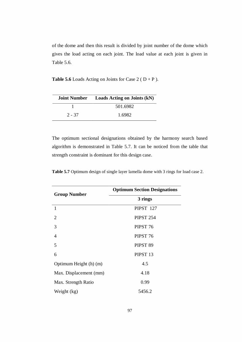
97
of the dome and then this result is divided by joint number of the dome which
gives the load acting on each joint. The load value at each joint is given in
Table 5.6.
Table 5.6 Loads Acting on Joints for Case 2 ( D + P ).
The optimum sectional designations obtained by the harmony search based
algorithm is demonstrated in Table 5.7. It can be noticed from the table that
strength constraint is dominant for this design case.
Table 5.7 Optimum design of single layer lamella dome with 3 rings for load case 2.
Joint Number Loads Acting on Joints (kN)
1 501.6982
2 - 37 1.6982
Group Number Optimum Section Designations
3 rings
1 PIPST 127
2 PIPST 254
3 PIPST 76
4 PIPST 76
5 PIPST 89
6 PIPST 13
Optimum Height (h) (m) 4.5
Max. Displacement (mm) 4.18
Max. Strength Ratio 0.99
Weight (kg) 5456.2

98
The optimum weight obtained from this case is heavier than the first case in
which the single layer lamella dome is subjected to only 500 kN equipment
load at its crown. This design is %35.25 heavier than the former case which has
the optimum weight of 4034.2 kg. The reason is that, the harmony search
algorithm assigns heavy sections to the some group members when the applied
loads acting on joints are increased. In the current case, algorithm chooses
heavier sections for group 2, 3 and 5 compared to the former case. In addition
to this, optimum height of the dome is changed and some differences for the
number of nonlinear analysis iterations are observed for optimum design in this
case as illustrated in Table 5.8.
Table 5.8 Elastic Critical Load Factor Iterations for optimum design of Case 2.
Load Factor Number of Nonlinear
Analysis Iterations
0.1 15
0.2 15
0.3 3
0.4 3
0.5 2
0.6 11
0.7 3
0.8 8
0.9 16
1.0 3
The optimum design of single layer lamella dome for this case is demonstrated
in Figures 5.8 and 5.9. It can be easily discerned from these figures that the

99
height of the dome is 4.5 m which is 1.75 m less than the former dome which
has the 6.25 m optimum height mentioned in load case 1.
Figure 5.8 3D view of optimum single layer lamella dome for Case 2.
Figure 5.9 Side view of optimum single layer lamella dome for Case 2.
20 m
2.43 m
3.97 m
4.50 m

100
5.3 CASE 3 ( D + P + W )
In this case, the dome with 3 rings is designed for the combination of dead
load, equipment load acting only on crown of the dome, and the wind load
calculated below. The design procedure of wind load (analytical procedure)
explained in part 6.5.3 of ASCE 7-05 is followed.
Basic Wind Speed V is taken from Figure 6-1 of ASCE 7-05.
V= 40 m/s (90 mph)
Wind Directionality Factor Kd is taken from Table 6.4 of ASCE 7-05.
Kd = 0.85 (for arched roofs)
Importance Factor I for the building is determined as 1.15 from Table 1.1 of
ASCE 7-05.
I = 1.15 (for building category III)
Exposure Category is assumed as C from the definitions given in part 6.5.6 of
ASCE 7-05.
Velocity Pressure Exposure Coefficient Kz is taken from Table 6.3 of ASCE
7-05.
The mean height of the roof is 13.125 m. (43.061 feet).
Kz = 1.055 (for exposure C and 43 ft height)

101
Topographic Factor Kzt is calculated from 2
1 2 3(1 )ztK K K K where K1, K2,
and K3 are taken from Figure 6-4 of ASCE 7-05.
It is assumed that there are a 2-D ridge with H/Lh = 0.30, 3-D escarpment with
x/Lh = 1.00 and 2-D ridge with z/Lh = 0.40 in the general topology, where;
H : Height of the hill or escarpment relative to the upwind terrain , in meter,
Lh : Distance upwind of crest to where the difference in the ground elevation is
half the height of the hill or escarpment, in meter,
K1 : Factor to account for shape of topographic feature and maximum speed-up
effect,
K2: Factor to account for reduction in speed-up with distance upwind or
downwind of crest,
K3: Factor to account for reduction in speed-up with height above local terrain,
x : Distance (upwind or downwind) from the crest to the building site, in meter,
z : Height above local ground level, in meter,
K1 = 0.43, K2 = 0.33, K3 = 0.30 (from Figure 6-4 of ASCE 7-05)
Kzt = (1 + 0.43x0.33x0.30)2 = 1.087
Gust Effect Factor G is taken as 0.85 directly by assuming the structure as
rigid from part 6.5.8 of ASCE 7-05.
G = 0.85

102
Enclosure Classification is assumed as enclosed, since all lateral and upper
parts of the building are closed and subjected to wind pressure directly.
Velocity Pressure qz is calculated by using the equation given in part 6.5.10 of
ASCE 7-05.
2 20.613* * * * * ( / )z z zt dq K K K V I N m (5.4)
qz = 0.613x1.055x1.087x0.85x402x1.15 (5.5)
qz = 1099.5 kN/m2
Internal Pressure Coefficients GCpi are found as +0.18 and –0.18 for
enclosed buildings from Figure 6-5 of ASCE 7-05. Two signed values (positive
and negative) are used according to the code. Plus and minus signs signify
pressures acting towards and away from the internal surfaces, respectively.
External Pressure Coefficients Cp are found from Figure 6-6 of ASCE 7-05.
The dome is assumed to be separated into three parts as shown in Figure 5.2,
such as windward quarter, center half and leeward quarter. Three different
external pressure coefficients for these three parts of the dome are calculated
with respect to rise-to-span ratio. The rise-to-span ratio, r is 6.25/20=0.3125 for
the dome in which the maximum height (h) of 6.25 m is considered for being
safe in wind load calculation, which is obtained from Case 1 with different
algorithm parameters rather than optimum solution.
Cp = 2.75r – 0.7 = 2.75x0.3125 – 0.7 = 0.16 (for windward quarter) (5.6)
Cp = -0.7 - r = -0.7 - 0.3125 = - 1.0125 (for center half) (5.7)
Cp = - 0.5 (for leeward quarter) (5.8)

103
Main Force Resisting Systems
Design wind pressure is calculated from Equation 6.17 of ASCE 7-05:
2( ) ( / )p i pip qGC q GC N m (5.9)
where;
q = qh for roofs, evaluated at height h,
qi = qh for roofs of enclosed buildings,
G : Gust effect factor,
Cp : External pressure coefficient from Figure 6-6 or Figure 6-8 of ASCE 7-05,
(GCpi): Internal pressure coefficient from Figure 6-5 of ASCE 7-05.
For windward quarter
- 48.378 N/m²
p = 1099.5 x 0.85 x (0.16) – 1099.5 x (±0.18) =
347.442 N/m²
For center half
-1144.1672 N/m2
p = 1099.5 x 0.85 x (-1.0125) – 1099.5 x (±0.18) =
-748.3472 N/m2
For leeward quarter
-665.1975 N/m2
p = 1099.5 x 0.85 x (-0.50) – 1099.5 x (±0.18) =
-269.3775 N/m2
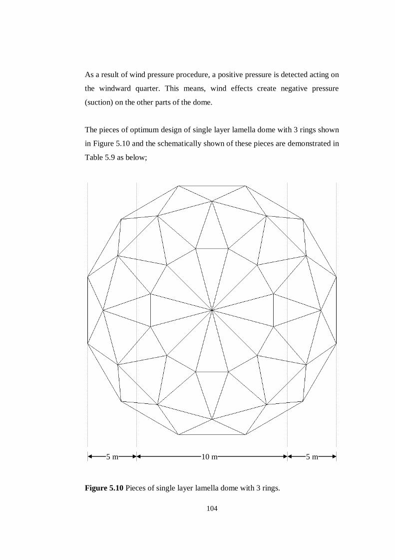
104
As a result of wind pressure procedure, a positive pressure is detected acting on
the windward quarter. This means, wind effects create negative pressure
(suction) on the other parts of the dome.
The pieces of optimum design of single layer lamella dome with 3 rings shown
in Figure 5.10 and the schematically shown of these pieces are demonstrated in
Table 5.9 as below;
Figure 5.10 Pieces of single layer lamella dome with 3 rings.
5 m 5 m 10 m
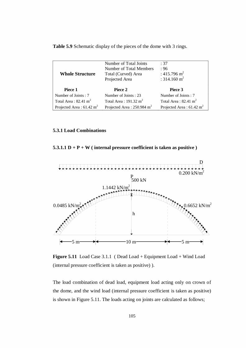
105
Table 5.9 Schematic display of the pieces of the dome with 3 rings.
Whole Structure
Number of Total Joints Number of Total Members
Total (Curved) Area
Projected Area
: 37 : 96
: 415.796 m2
: 314.160 m2
Piece 1 Piece 2 Piece 3
Number of Joints : 7 Number of Joints : 23 Number of Joints : 7
Total Area : 82.41 m2 Total Area : 191.32 m2 Total Area : 82.41 m2
Projected Area : 61.42 m2 Projected Area : 250.984 m2 Projected Area : 61.42 m2
5.3.1 Load Combinations
5.3.1.1 D + P + W ( internal pressure coefficient is taken as positive )
Figure 5.11 Load Case 3.1.1 ( Dead Load + Equipment Load + Wind Load
(internal pressure coefficient is taken as positive) ).
The load combination of dead load, equipment load acting only on crown of
the dome, and the wind load (internal pressure coefficient is taken as positive)
is shown in Figure 5.11. The loads acting on joints are calculated as follows;
0.200 kN/m2
P
D
500 kN
h
10 m 5 m 5 m
1.1442 kN/m2
0.6652 kN/m2 0.0485 kN/m
2

106
For windward quarter
P = ( -0.200 x 61.42 + ( 0.0485 x cos (43.17)o x 82.41 ) / ( 7 joints )
= -1.3381 kN / joint ( )
P = ( ( -0.0485 x sin (43.17)o) x 82.41 ) / ( 7 joints )
= -0.391 kN / joint ( )
For Center Half
P = ( -0.200 x 191.32 ) / ( 23 joints ) = -1.664 kN / joint ( )
P = ( 1.1442 x 250.984 ) / ( 23 joints ) = 12.486 kN / joint ( )
10.822 kN / joint ( )
For Leeward Quarter
P = ( -0.200 x 61.42 + ( 0.6652 x cos (43.17)o ) x 82.41 ) / ( 7 joints )
= 3.957 kN / joint ( )
P = ( ( 0.6652 x sin (43.17)o ) x 82.41 / ( 7 joints )
= 5.358 kN / joint ( )
The results obtained for the optimum design of this loading case is given in
Table 5.10.

107
Table 5.10 Optimum design obtained for dome with 3 rings for the case
D + P + W (internal pressure coefficient is taken as positive).
The optimum dome for this loading case is a little lighter than the precedent
one which has 5456.2 kg as optimum weight and is subjected to combination of
dead load and equipment load at its crown. The Harmony Search algorithm
selects different sections for the groups of 2, 4 and 5 for this case when it is
compared with former loading case. The strength constraint is dominant and
very close to one as can be seen in the above table. The optimum heights of
previous design and this one are same. The elastic critical load factor iterations
for optimum designed single layer lamellar dome according to this loading case
are presented in Table 5.11.
Table 5.11 Elastic Critical Load Factor Iterations for optimum design of
loading case D+P+W (internal pressure coefficient is taken as positive ).
Load Factor 0.1 0.2 0.3 0.4 0.5 0.6 0.7 0.8 0.9 1.0
Number of Nonlinear Analysis
Iterations 3 2 2 2 2 2 2 2 1 2
Group Number Optimum Section Designations
3 rings
1 PIPST 127
2 PIPST 203
3 PIPST 76
4 PIPST 89
5 PIPST 102
6 PIPST 13
Optimum Height (h) (m) 4.5
Max. Displacement (mm) 4.3
Max. Strength Ratio 0.98
Weight (kg) 5412.4
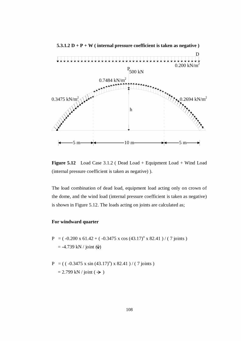
108
5.3.1.2 D + P + W ( internal pressure coefficient is taken as negative )
Figure 5.12 Load Case 3.1.2 ( Dead Load + Equipment Load + Wind Load
(internal pressure coefficient is taken as negative) ).
The load combination of dead load, equipment load acting only on crown of
the dome, and the wind load (internal pressure coefficient is taken as negative)
is shown in Figure 5.12. The loads acting on joints are calculated as;
For windward quarter
P = ( -0.200 x 61.42 + ( -0.3475 x cos (43.17)o x 82.41 ) / ( 7 joints )
= -4.739 kN / joint ( )
P = ( ( -0.3475 x sin (43.17)o) x 82.41 ) / ( 7 joints )
= 2.799 kN / joint ( )
10 m 5 m 5 m
P 0.200 kN/m
2
D
500 kN
h
0.7484 kN/m2
0.2694 kN/m2 0.3475 kN/m
2

109
For Center Half
P = (-0.200 x 191.32 + 0.7484 x 250.984 ) / ( 23 joints ) = -6.503 kN / joint ( )
For Leeward Quarter
P = ( -0.200 x 61.42 + ( 0.2694 x cos (43.17)o ) x 82.41 ) / ( 7 joints )
= 0.559 kN / joint ( )
P = ( ( 0.2694 x sin (43.17)o ) x 82.41 / ( 7 joints )
= 2.169 kN / joint ( )
The results obtained for the optimum design of this loading case is given in
Table 5.12.
Table 5.12 Optimum design for dome with 3 rings for D + P + W ( internal
pressure coefficient is taken as negative ) .
Group Number Optimum Section Designations
3 rings
1 PIPST 152
2 PIPST 203
3 PIPST 76
4 PIPST 76
5 PIPST 102
6 PIPST 13
Optimum Height (h) (m) 3.5
Max. Displacement (mm) 3.53
Max. Strength Ratio 0.98
Weight (kg) 5390.5

110
According to Table 5.12, the optimum dome under this loading case is lighter
than the previous two cases which are D + P and D + P + W (internal pressure
coefficient is taken as positive). The strength constraint is dominant and the
optimum height of the dome is less than the height of previous two designs 4.5
m. The elastic critical load factor iterations for optimum designed single layer
lamellar dome according to this loading case are shown in Table 5.13;
Table 5.13 Elastic Critical Load Factor Iterations for optimum design of
loading case D+P+W ( internal pressure coefficient is taken as positive ).
Load Factor 0.1 0.2 0.3 0.4 0.5 0.6 0.7 0.8 0.9 1.0
Number of
Nonlinear Analysis
Iterations
6 2 2 2 1 2 7 2 1 2
The elevations of the optimum domes for all load cases are shown in Figures
5.13 - 5.15.
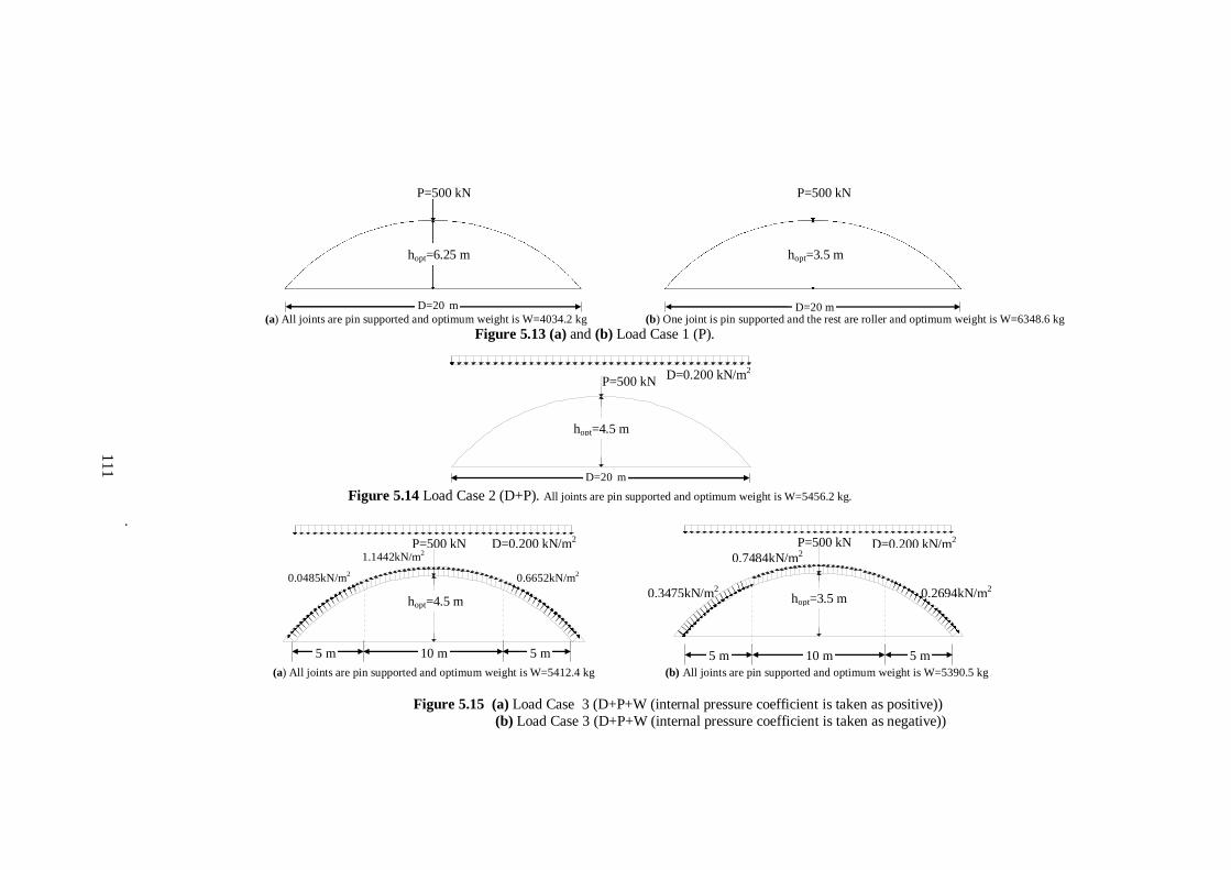
P=500 kN
hopt=4.5 m
D=0.200 kN/m2
D=20 m
P=500 kN D=0.200 kN/m2
1.1442kN/m2
0.0485kN/m2
0.6652kN/m2
hopt=4.5 m
5 m 5 m 10 m
P=500 kN
hopt=6.25 m
D=20 m
P=500 kN
hopt=3.5 m
D=20 m
111
(a) All joints are pin supported and optimum weight is W=4034.2 kg (b) One joint is pin supported and the rest are roller and optimum weight is W=6348.6 kg
Figure 5.13 (a) and (b) Load Case 1 (P).
Figure 5.14 Load Case 2 (D+P). All joints are pin supported and optimum weight is W=5456.2 kg.
.
(a) All joints are pin supported and optimum weight is W=5412.4 kg (b) All joints are pin supported and optimum weight is W=5390.5 kg
Figure 5.15 (a) Load Case 3 (D+P+W (internal pressure coefficient is taken as positive))
(b) Load Case 3 (D+P+W (internal pressure coefficient is taken as negative))
P=500 kN D=0.200 kN/m2
hopt=3.5 m
0.7484kN/m2
0.2694kN/m2 0.3475kN/m2
5 m 10 m 5 m

112
CHAPTER 6
CONCLUSIONS
In this thesis, the optimum topological design problem of geometrically
nonlinear single layer lamella domes is considered. The design problem is
formulated such that the total number of rings, the height of the crown, and the
steel pipe section designations required for the member groups in the dome are
treated as design variables. The design limitations that consist of serviceability
and strength constraints are implemented from LRFD-AISC. Furthermore, the
geometric nonlinearity of the dome structure is also taken into account and
elastic critical load factor analysis is carried out for each candidate dome
structure to make sure that the dome does not lose its stability under the
external loading. The mathematical model of the programming problem
obtained is discrete, complex, and highly nonlinear. The Harmony Search
method which is one of the recent addition to stochastic search techniques of
numerical optimization is used to obtain the solution of the design problem. It
is shown in the design examples considered that the harmony search method
can be used in finding the solution of optimum topology problem where the
topology, shape and size of members in a structure are taken as design variable.
However, three main parameters of the algorithm namely, harmony memory
size HMS, harmony memory considering rate HMCR, and the pitch adjustment
rate PAR are required to be selected before the harmony search method
initiates its search for the optimum solution. It is shown that the appropriate
values of these parameters are problem dependent and one set of values which
gives good results in one design problem may not lead to a good solution in
another problem. It is therefore necessary to carry out a number of runs with

113
different values of these parameters and determine the suitable ones that yield
the lightest structure.
It is shown that the nonlinear displacements of a lamellar dome can be more
than 10% of the linear displacements under the same loading. This clearly
justifies that consideration of the geometrical nonlinear behavior in the
optimum design of such structures is a necessity. This not only provide
inclusion of the realistic behavior of these structures, but also results in further
reduction in the optimum weight. Support conditions also affect the optimum
design of lamellar domes. The optimum weight of the dome with roller type
supports becomes 57.4% heavier than the dome where supports are all pinned.

114
REFERENCES
[1] Benjamin, B.S. (1962). “The Analysis of Braced Domes.” Asia.
[2] Rao, S.S. (1996). “Engineering Optimization: Theory and Practice.”
Wiley-Interscience.
[3] Saraç, Y. (2005). “Optimum Design of Pin-Jointed 3-D Dome
Structures Using Global Optimization Techniques.” MSc Thesis, METU.
[4] Arora, J.S. (Editor) (1997). “Guide to Structural Optimization.” ASCE.
[5] Shapiro, J.F. (1979). “Mathematical programming:structures and
algorithms.” Wiley.
[6] Venkayya, V. B., Khot, N. S., and Berke, L. (1973). “Application of
Optimality Criteria Approaches to Automated Design of Large Practical
Structures.” Second Symposium Structural Optimization, AGARD-CP-123,
Milan, Italy.
[7] Goldberg, D.E. (1989). “Genetic Algorithms in search, optimization,
and machine learning.” Addison-Wesley Publishing Company.
[8] Holland, J.H. (1992). “Adaption in natural and artificial systems: an
introductory analysis with applications to biology, control, and artificial
intelligence.” Cambridge, Mass: MIT Press.
[9] Rechenberg, I. (1973). “Evolutionsstrategie, Optimierung technischer
Systeme nach Prinzipien der biologischen Evolution.” Frommann-Holzboog.

115
[10] Schwefel, H.P. (1981). “Numerical Optimization of Computer Models.”
Wiley.
[11] Langdon, W.B., and Qureshi, A. (1995). “Genetic Programming-
Computer Using “Natural Selection” to Generate Programs.” RN/95/76,
http://www.citeseer.ist.psu.edu/langdon95genetic.html. Last accessed date
April 20th
, 2008.
[12] Schneider, J.J., and Kirkpatrick, S. (2006). “Stochastic Optimization.”
Springer.
[13] Camp, C.V., and Bichon, B.J. (2004). “Design of Space Trusses Using
Ant Colony Optimization.” Journal of Structural Engineering, 130, 741-751.
[14] Glover, F. (1986). “Future Paths For Integer Programming and Links
to Artificial Intelligience.” Comp & Oper. Res., 13, 533-549.
[15] Aguirre-Solis, J.J. (1999). “Tabu Search Algorithm For The Open Shop
Scheduling Problem With Sequence Dependent Setup Times.” The Society
For Modeling and Simulation International (SCS).
http://www.scs.org/getDoc.cfm?id=2172. Last accessed date April 16th, 2008.
[16] Geem, Z.W., Kim, J-H., and Loganathan, G.V. (2001). “A new
heuristic optimization algorithm: Harmony Search.” Simulation, 76, 60-80.
[17] Lee, K.S., and Geem, Z.W. (2004). “A new structural optimization
method based on the harmony search algorithm.” Computers and Structures,
82, 781-798.

116
[18] Saka, M.P. (1990). “Optimum Design of Pin-Jointed Steel Structures
with Practical Applications.” Journal of Structural Engineering, ASCE, 116,
10, 2599-2690.
[19] Saka, M.P., and Ulker, M. (1992). “Optimum design of geometrically
nonlinear space trusses.” Computer and Structures, 42, 3, 289-299.
[20] Huyber, P. (1995). “Super-Elliptic Geometry as a Design Tool for the
Optimization of Dome Structures.” Structural Systems and Industrial
Applications, 387-399.
[21] Saka, M.P., and Kameshki, E.S. (1998). “Optimum design of nonlinear
elastic framed domes.” Advances in Engineering Software, 29, 7-9, 519-528.
[22] Erbatur, F., Hasançebi, O., Tütüncü, Ġ., and Kılıç, H. (2000). “Optimal
design of planar and space structures with genetic algorithms.” Computers and
Structures, 75, 209-224.
[23] Lin, S.P., and Albemani, F. (2001). “Lattice-Dome Using a Knowledge-
Based System Approach.” Computer-Aided and Infrastructure Engineering, 16,
268-286.
[24] Ulker, M., and Hayalioğlu, M.S. (2001). “Optimum design of Space
Trusses with Buckling Constraints by means of Spreadsheets.” Turk J. Engin.
Environ. Sci., 25, 355-367, TUBITAK.
[25] Missoum, S., Gürdal, Z., and Gu, W. (2002). “Optimization of
nonlinear trusses using a displacement-based approach.” Struct. Multidisc.
Optim., 23, 214-221.

117
[26] Khot, N.S., and Kamat, M.P. (1985). “Minimum weight design of truss
structures with geometric nonlinear behavior.” AIAA Journal, 23, 139-144.
[27] Yuan, X.F., and Dong, S.L. (2002). “Nonlinear analysis and optimum
design of cable domes.” Engineering Structures, 24, 965-977.
[28] Rajasekaran, S., Mohan, V.S., and Khamis, O. (2004). “The
optimisation of space trusses using evolution strategies with functional
networks.” Engineering with Computers, 20, 75-87.
[29] Lingyun, W., Mei, Z., Guangming, W. and Gang, M. (2005). “Truss
optimization on shape and sizing with frequency constraints based on genetic
algorithm.” Comput. Mech., 35, 361-368.
[30] Kitipornchai, S., Kan, W., Lam, H-F., and Albermani, F. (2005).
“Factors affecting the design and construction of Lamella suspen-dome
systems.” Journal of Constructional Steel Research, 61, 764-785.
[31] Toğan, V., and Daloğlu, A.T. (2006). “Optimization of 3D trusses with
adaptive approach in genetic algorithms.” Engineering Structures, 28, 1019-
1027.
[32] Lόpez, A., Puente, I., and Serna, M.A. (2007). “Numerical model and
experimental tests on single-layer latticed domes with semi-rigid joints.”
Computers and Structures, 85, 360-374.
[33] Kameshki, E.S., and Saka, M.P. (2007). “Optimum geometry design of
nonlinear braced domes using genetic algorithm.” Computers and Structures,
85, 71-79.

118
[34] Saka, M.P. (2007). “Optimum topological design of geometrically
nonlinear single layer latticed domes using coupled genetic algorithm.”
Computers and Structures, 85, 21-22, 1635-1646.
[35] Coates, R.C., Coutie, M.G., and Kong, F.K. (1972). “Structural
Analysis” Nelson.
[36] Ekhande, S.G.i Selvappalam, M., and Madugula, K.S. (1989). “Stability
Functions for Three-Dimensional Beam-Columns.” Journal of Structural
Engineering, 115, 2, 467-479.
[37] Saka, M.P. (2007). “Optimum Geometry Design of Geodesic Domes
Using Harmony Search Algorithm.” Advances in Structural Engineering, 10, 6,
595-606.
[38] Manual of Steel Construction. (1991). “LRFD, Volume 1, Structural
Members, Specifications & Codes.” American Institute of Steel Construction
Inc.
[39] Galambos, T.V, Lin, F.J., and Johnston, B.G. (1996). “Basic Steel
Design with LRFD.” Prentince Hall.
[40] Lee, K.S., Geem, Z.W. (2005). “A new meta-heuristic algorithm for
continuous engineering optimization: harmony search theory and practice.”
Computer methods in applied mechanics and engineering, 194, 3902-3933.