Optimizing the design of complex energy conversion

systems by Branch and Cut

Turang Ahadi-Oskui1, Stefan Vigerske2,3,Ivo Nowak2, and George Tsatsaronis1

June 5, 2010

Abstract

The paper examines the applicability of mathematical programming methods tothe simultaneous optimization of the structure and the operational parameters of acombined-cycle-based cogeneration plant. The optimization problem is formulated asa non-convex mixed-integer nonlinear problem (MINLP) and solved by the MINLPsolver LaGO. The algorithm generates a convex relaxation of the MINLP and ap-plies a Branch and Cut algorithm to the relaxation. Numerical results for differentdemands for electric power and process steam are discussed and a sensitivity analysisis performed.

1 Introduction

The design of large-scale energy conversion systems is a highly complex process even whenonly the steady-state case is considered. Design optimizations for new projects are of-ten limited to sensitivity analyses of existing plants or application of heuristic rules [3–5, 7, 10, 20, 26, 30]. The increasing computing power and the further development of opti-mization algorithms in the last years allow now the application of novel computer-aidedtools [3,4,15–17,27]. This paper examines the applicability of mathematical programmingmethods to the optimization of the design of a combined-cycle-based cogeneration plant.The optimization is not only limited to operational parameters alone, but also searches foran appropriate structure of the plant. The goal of the optimization is to find a plant designwith minimum levelized total cost that fulfills the user specified demands for electric powerand process steam.

The presence of integer variables (to model the structure of the plant) and nonlinearequations (to model the thermodynamic behavior of the components), leads to a formu-lation of the optimization problem as mixed-integer nonlinear program (MINLP). The

1Technical University Berlin, Institute for Energy Engineering, Marchstr. 18, 10587 Berlin, Germany2Humboldt University Berlin, Department of Mathematics, Unter den Linden 6, 10099 Berlin, Germany3Corresponding author. E-Mail: stefan@math.hu-berlin.de

1

discrete decisions and nonconvexity of some equations requires the application of sophisti-cated global search methods since – due to the potential presence of several local optimalsolutions – traditional methods for convex optimization do not guarantee to find a globaloptimal solution as well as a valid bound on the global optimal value. In this paper, theMINLP solver LaGO (Lagrangian Global Optimizer) [23, 24] was used to optimize thedesign of an energy conversion system.

In the next section, we introduce our model of a combined-cycle-based cogenerationplant. Section 3 describes the solution algorithm that was applied here. Section 4 presentssome numerical results.

2 Optimization Problem

2.1 Combined-cycle based cogeneration plant

The energy conversion system analyzed here is based on a combined-cycle process, whichis a combination of a gas turbine process with a steam turbine process [3,5,18], see Figure1 for a simple configuration. For cogeneration plants running in a stationary operationmode, the entire fuel is generally fed to the gas turbine which represents the topping cycleand produces about 2/3 of the electric power of the overall process. The energy of the gasturbine exhaust gas is used within a heat recovery steam generator (HRSG) to producesuperheated steam. The steam is fed to a steam turbine to generate additional electricpower. Since the steam turbine process operates at a lower temperature level, it is calledthe bottoming cycle. The combination of both processes working at different temperaturelevels allows a very efficient utilization of the fuel energy. With an efficiency of up to 59%,combined-cycle processes reach the highest efficiency for the production of electric powerfrom fossil fuels today. Looking at the environmental perspective, in addition to the highefficiency, the use of natural gas as fuel contributes to relatively low specific CO2-emissions.

A combined-cycle process can easily be converted into a cogeneration plant, in whichprocess steam is produced in addition to electric power. The required steam is extractedfrom the steam cycle, in general from a steam turbine stage, at an appropriate pressure.

2.2 Superstructure

The goal of the optimization is to find a design of the combined-cycle-based cogenerationplant with minimum levelized total costs. Starting point for the simultaneous optimizationof the structure and the process variables of the design is a so-called superstructure. Thesuperstructure of the cogeneration plant represents a superior process flow sheet whichcombines a variety of different plant designs. It contains all possible plant components,necessary for accomplishing the predefined task, and all possible connections between them.Depending on the user-specified electric power and process steam demands, the optimiza-tion algorithm finds an optimized structure within the superstructure and the associatedvalues of the process variables. The superstructure was developed by combining various

2

Air

Fuel

Exhaust Gas

Gas Turbine

Heat RecoverySteam Generator

Steam Turbine

Process

Steam

Figure 1: Schematic representation of a combined-cycle power plant with steam extraction

existing combined-cycle plant designs and considering all features that in our opinion havethe potential for improving the effectiveness of the overall plant. The superstructure wasdesigned for an electric power output between 50 MW and 400 MW and a process steamproduction of up to a total of 500 t/h at up to three different pressure levels. A specificdesign is determined by a set of 28 binary structural variables and 48 continuous pro-cess variables. A structural variable decides over the existence of a plant component ora stream connection whereas the process variables specify mass flow rates, temperatures,and pressures of process streams as well as efficiencies of plant components.

A superstructure of the present complexity cannot be displayed concisely in one coher-ent process flow sheet. Therefore, the superstructure is divided into three parts: the gasturbine system, the water-steam-cycle, and the exhaust gas path. Figures 2, 3, and 4 showthe considered plant components (numbered from 501 to 533) and the process streams inbetween them. The structural decisions are represented by dots, which mark either an“and” decision or an “or” decision. In the following, they are discussed in more details.

2.2.1 Gas Turbine

Contrary to industrial standards, the gas turbine system is not a fixed system but is com-posed of individual components to be designed, see Figure 2 for a process flow sheet. Thisincreases the flexibility for the optimization and allows the creation of innovative designs.The first structural option determines whether intercooling with staged compression shouldbe included into the design or not. The intercooling can be realized by an injection cooler(Component No. 503 in Figure 2) or by a surface heat exchanger (502). Before enteringthe combustion chamber, the compressed air can be preheated in an air preheater (505).

3

During the expansion process, reheating of the exhaust gas can be realized in a secondcombustion chamber (508). The remaining structural variables for the gas turbine sys-tem decide over fuel preheating (510) and a possible steam injection into each combustionchamber. The streams at the bottom part of the flowsheet represent the cooling air for theturbine blades. The exhaust gas stream is finally fed to the HRSG.

Air

Fuel

HRSG

SteamSteam

Compressor

Injection Cooler

Surface Intercooler

Air Preheater

Combustion Chamber Fuel Preheater

2nd-Stage Compressor Sequential Combustion Chamber

Expander

2nd-Stage Expander

HRSG Heat Recovery Steam Generator

501

502

503 504505

506

507508

509

510

501

502

503

504

505

506

507

508

509

510

Figure 2: Gas turbine part of the superstructure

2.2.2 Water/Steam Cycle

The water-steam-cycle consists of the water-side of the HRSG, the steam turbines, and thecondensing part including the feedwater tank. The flowsheet for the water/steam cycle isshown in Figure 3. Steam can be produced at up to three different pressure levels (high,medium, and low). The medium- and low-pressure levels are optional and their existenceis determined by structural variables. Each pressure level consists of a feedwater pump, aneconomizer, an evaporator, and a superheater. The economizer of the low-pressure level(522) and the superheaters of the low- and medium-pressure levels (520 and 517) representalso structural decisions. The generated steam is expanded in up to three steam turbineswhereas the medium-pressure steam turbine and the associated reheater are optional. Ifrequired, process steam can be extracted at four different locations (PD1 to PD4). Afterthe condensate pump, there is an option to implement a condensate reheater (523).

4

PD 1

I

II

III

IV

V

VI

VII

VIII

521524

526

510

512515516

517

518519

520

522

525

533

I

II

III

IV

V

VI

VII

VIII

PD 2

GT

PD 3 PD 4

ZW528

531

514 523527

529529

530

533

PD 1

HP-Superheater

Feedwatertank

LP-Pump

LP-Economizer

LP-Evaporator

LP-SuperheaterFuel Preheater

HP-Evaporator

HP-Economizer

MP-Superheater

MP-Evaporator

MP-Economizer

MP-Pump

HP-Pump

Process Steam Extraction 1510

512

515

516

517

518

519

520

522

525

533

521

524

526

ZW

GT

PD 2

PD 3

PD 4Reheater

Condensate Economizer

HP-Steam Turbine

MP-Steam Turbine

LP-Steam Turbine

Condenser

Condensate Pump

Process Steam Extraction 2

Process Steam Extraction 3

Process Steam Extraction 4

Gas Turbine

Additional Water

514

523

527

529

530

528

531

HP: High Pressure MP: Medium Pressure LP: Low Pressure

Figure 3: Water-steam-cycle of the superstructure

2.2.3 Exhaust Gas Path

The exhaust gas path represents the gas-side of the HRSG. In Figure 4, every rectangledenotes a surface heat exchanger. The structural variables determine the configuration ofthe heat exchangers (order, in series, or in parallel). The path through the HRSG is, ofcourse, coupled to the existence of steam at the low- or medium-pressure levels. Finally,there is an option to implement up to two duct burners (511, 513) into the HRSG.

5

HR

Fuel

HS

HV

HE ME

MV

KV

NE

NV

NSMS

Reheater

HP Superheater

HP Evaporator

HP Economiser

MP Superheater

MP Evaporator

MP Economiser

LP Superheater

LP Evaporator

LP Economiser

Condensate Preheater

fromGas Turbine

HP: High Pressure

MP Economiser

MP: Medium Pressure

LP Economiser

LP: Low Pressure

HS

HR

HSHE

MS HE

MS

NS MV

ME

NS

NS ME

ME

HE

NS

HR

HV HE

MS

MV ME NS NV NE KV511

512

513

514515

516517

518 519

513

512

514

516

516

517

517

516

518

519

519

519

520

521 522 523

520

520

520

520

Fuel

Fuel

Figure 4: Exhaust gas path through the HRSG of the superstructure

2.3 Model of the superstructure

The model of the superstructure describes the thermodynamic behavior of the cogenerationplant, performs the economic analysis and yields the levelized total costs for the overallplant. The equations of the model can be divided into different categories. The first cate-gory of equations describes the logic of the superstructure, i.e., how the plant componentsare connected to each other, under which conditions the different setups are possible, andwhich restrictions have to be fulfilled in each case.

The second category of equations consists of the models that specify the thermodynamicbehavior of the plant components. The models of the plant components should on one sidebe kept as simple as possible, to facilitate the work of the optimization algorithm and toshorten the total computing time. On the other side, they have to guarantee a certain levelof accuracy. The model of a plant component consists of mass and energy balances as wellas characteristic functions which describe the thermodynamic behavior of the component.

To simulate the behavior of the plant components, thermodynamic property equationsfor all substances and mixtures used in the plant (e.g., exhaust gas, water, and steam) areneeded. The exhaust gas is treated as an ideal mixture of ideal gases and the propertiesare calculated using the equations given in [19].

The third category of equations is formed by the functions approximating the purchaseequipment costs. These functions represent the most imprecise part of the model sincereal cost data are hardly available. In this work we use cost functions either from theliterature [5, 31] or derived from available cost data [8, 13].

The last category of equations belongs to financial mathematics. With these equationsthe economic analysis, which yields the levelized total costs for the cogeneration plant,is conducted. The cost of the plant represents the total revenue which is required to

6

maintain a sound economic operation of the plant. The total cost consists of investmentcost, operating and maintenance cost, fuel cost, depreciation, taxes, insurance, interests,and a minimum return on investment. The economic analysis is performed according tothe Total Revenue Requirement (TRR) method [5]. The levelization of the costs takes thetime value of money into account.

The model for the MINLP solver LaGO is programmed as one coherent system ofequations using the mathematical modeling language GAMS [12]. Since the MINLP solverrequires first and second derivatives of the equations of the model, external software (e.g.,for the simulation of single components of the plant) cannot be employed. The complexityof the integrated nonlinear and nonconvex functions is limited to a certain degree to assurethe convergence of the solver. Therefore, for calculating the properties of water and steamin LaGO, the IAPWS-IF 97 functions [32] with up to 60 terms and exponents of ±50 areapproximated by less complicated polynomials of lower degree.

Another restriction of the mathematical programming algorithm is that the designercannot determine a calculation sequence because the entire model is computed simulta-neously. Here, distinction of cases can only be realized by additional binary variables,which increase the complexity of the problem. Moreover, even though inactive parts of themodel have to be decoupled from the objective function, the equations of inactive plantcomponents have to be satisfied anyhow.

Modeling the overall plant performance with a system of equations has advantages inconjunction with recirculated streams because there is no need for the designer to determinea calculation order. Moreover, additional plant components can be easily integrated intothe model by connecting them with the upstream and downstream components.

Due to great differences in the order of magnitude of the variables, the entire model ofthe superstructure has to be scaled to ensure an equal treatment by the solver regardingthe compliance of all equations. In addition, to facilitate the work of the solver and toimprove the quality of the results, upper and lower bounds for all variables of the model areneeded. This causes significant additional work for a model with 1308 variables and 1640constraints. The optimization is controlled by the MINLP solver LaGO which accessesthe GAMS model of the superstructure, performs the optimization, and stores the bestsolutions of a run in a data file for a subsequent analysis.

3 MINLP optimization by Branch and Cut

In this section we briefly describe the algorithm that is used to solve the design prob-lem described in Section 2. The model can be formulated as the following mixed-integernonlinear program (MINLP):

min bT0 x

such that h(x) ≤ 0,x ∈ [x, x],xj ∈ {0, 1} , j ∈ B,

(P)

7

where B ⊆ {1, . . . , n}, c, x, x ∈ Rn, x ≤ x, and h : R

n → Rm is twice continuously

differentiable. Without loss of generality, we have assumed a linear objective function hereand replaced equality constraints by two inequalities in this general formulation.

If the function h(x) in (P) is convex, then the MINLP is denoted as convex MINLP.There are mainly three approaches for the solution of convex MINLPs. In successiveouter-approximation algorithms [9, 11], a mixed-integer linear (MIP) relaxation of (P) isconstructed and successively improved by linearizing h(x) in several points. The optimalvalue (or a lower bound on it) of this outer-approximation yields a valid lower bound forthe optimal value of (P). The relaxation is thereby solved by a MIP solver, which usuallyemploys a Branch and Cut algorithm. The optimal solution of the MIP relaxation furtherserves as a starting point for a local search in the NLP that is obtained by fixing thebinary variables in (P) to the values in the solution of the MIP relaxation. Solutions thatare feasible in this NLP provide also feasible solutions for (P), and, hence, yield an upperbound on the optimal value of (P). An extension of this outer-approximation algorithmconsists of integrating the construction of the outer-approximation into the Branch andCut algorithm that is used to solve the MIP relaxation [25]. This algorithm is especiallyuseful for models with a difficult combinatorial part. A third approach for solving convexMINLPs is the replacement of the linear relaxation as used in a classical Branch and Boundalgorithm for MIPs by a nonlinear (continuous) relaxation [21]. This nonlinear relaxationof (P) is obtained by relaxing the binary conditions on xj , j ∈ B, to bound constraintsxj ∈ [0, 1], j ∈ B. The solution of this NLP yields a lower bound on the optimal valueof (P). If, further, all variables xj , j ∈ B, take integral values, then also a feasiblesolution for (P) (and thus an upper bound on the optimal value of (P)) has been found.However, if some binary variables take fractional values in the NLP relaxation, then twonew subproblems are generated by fixing a single binary variables to 0 and 1, respectively(branching). The algorithm is then applied recursively to this subproblem.

However, if h(x) is not convex, then these algorithms cannot be applied in a straightforward manner, since linearizations of h(x) usually do not yield an outer-approximationand the NLP solvers employed for solving NLP relaxations usually guarantees global op-timal solutions only for convex problems. Therefore, for the global solution of noncon-vex MINLPs, convexification techniques and spatial Branch and Bound algorithms areemployed. Convexification techniques [1, 29] generate linear or convex nonlinear underes-timators of nonconvex functions, which can be utilized for the construction of linear orconvex nonlinear relaxations of (P). The tightness of an underestimator thereby dependsstrongly on the bounds on the variables – as tighter the bounds as better is the underesti-mator. Thus, subdividing a problem into subproblems with smaller ranges for a continuousvariable (that is involved in a nonconvex function) allows to tighten a convex relaxation.This leads to spatial Branch and Bound algorithms as they are implemented in solvers likeBARON [28], Couenne [6], and LaGO [23,24].

In this paper, the Branch and Cut algorithm that is implemented in the MINLP solverLaGO (Lagrangian Global Optimizer) was used to solve the model introduced in Section 2.We assume to have procedures for evaluating function values, gradients, and Hessians ofthe functions hi(x), i = 1, . . . , m. The restriction to black-box functions has the advantage

8

that our algorithm can handle more general functions than other deterministic solvers fornonconvex MINLPs. On the other hand, we are not able to use advanced convexificationand box reduction techniques (as in [22,29]). Hence, for some components of our algorithm,e.g., Section 3.2.1, we are restricted to use less rigorous sampling methods.

The proposed algorithm follows a Branch and Bound scheme to search for a globaloptimum of (P). It starts by considering the original problem with its complete feasibleregion, which is called the root problem. A lower bound on the global optimum of (P) iscomputed by solving a linear outer-approximation of (P). An upper bound v is computedby finding a local optimum of (P). If the bounds match, a globally optimal solution hasbeen found and the procedure terminates. Otherwise, two new problems are constructedby dividing the feasible region of (P) (branching). The new problems become “children”of the root problem, and the algorithm is applied recursively on each subproblem. Thisprocess constructs a tree of subproblems, the Branch and Bound tree.

The gap between the lower bound v(U) of a node U and the global upper bound v isdiminished by improving the linear outer-approximation and by computing local optimalpoints. If such a point is found and the upper bound v is improved, nodes of the tree, thelower bound of which exceeds v, are pruned. The process of branching and bounding isperformed until no unprocessed nodes are left or the gap has been sufficiently reduced.

The linear outer-approximation of (P) is based on a (nonlinear) convex outer-approxi-mation (C). It is obtained by the following steps:

1. Check functions for block-separability, i.e., whether they can be written as a sum offunctions each depending only on a small number of variables, c.f. Section 3.1. Block-separability is exploited by LaGO for the construction of relaxations and during boxreduction.

2. Identify convex and quadratic functions, c.f. Section 3.2.

3. Underestimate nonconvex nonquadratic functions by quadratic functions, c.f. Sec-tion 3.2.1. This step is a preparation for the following convexification step.

4. Construct a convex relaxation (C) of (P) by taking all linear and convex nonlinearconstraints from (P) (as identified in Step 2). Add convex underestimators for allremaining quadratic constraints (coming either directly from (P) or generated inStep 3), c.f. Section 3.2.2.

5. Generate a linear outer-approximation (R[U ]) by linearizing the constraints of theconvex relaxation (C), c.f. Section 3.2.3.

The tightness of the convex underestimators for quadratic functions (Step 4) is deter-mined by the ranges of the variables. Thus, to improve the efficiency of the algorithm,box reduction techniques which aim on deducing reduced variable bounds from the set ofconstraints and given variable bounds are applied. This allows to tighten the box [x, x] (ora subbox) and can discover infeasibility of subproblems during branch-and-bound.

In the following, we briefly explain the above mentioned components of the algorithm.For more details we refer to [24]. A list of symbols used in this section is given in Table 1.

9

Table 1: List of Symbols

Optimization problems

(P) original MINLP(Q) “pre-convex” relaxation, cf. Section 3.2.1(C) the convex relaxation, cf. Section 3.2.2(R) linear relaxation, cf. Section 3.2.3(R[U ]) linear relaxation for a subbox U ⊆ [x, x], cf. Section 3.2.3(Bj [U ]) auxiliary problem to compute bounds on variable xj , cf. Section 3.3

Problem formulation

b0 objective function coefficients, b0 ∈ Rn

h(x) constraint functions, h : Rn → R

m

x lower bounds on variables, x ∈ Rn

x upper bounds on variables, x ∈ Rn

[x, x] box of admissible variable values, [x, x] := {x ∈ Rn : xi ∈ [xi, xi], i = 1, . . . , n}

B indices of binary variables, B ⊆ {1, . . . , n}xI subvector (xi)i∈I ∈ R

|I| for an index set I ⊆ {1, . . . , n}

Block-separable reformulation (cf. Section 3.1)

ci constant part of constraint i, ci ∈ R

bi coefficients of linear part of constraint i, bi ∈ Rn

Qi,k indices of variables in the k’th quadratic function block of constraint iqi number of quadratic function blocks of constraint iAi,k coefficients of k’th quadratic function block of constraint i, Ai,k ∈ R

|Qi,k|×|Qi,k|

Ni,k indices of variables in the k’th nonlinear nonquadratic function block of con. ihi,k k’th nonlinear nonquadratic function of constraint i, hi,k : R

|Ni,k| → R

pi number of nonlinear nonquadratic function blocks of constraint i

Convexification and Linearization

q(x) a quadratic underestimator, cf. Section 3.2.1α convexification parameter of an α-underestimator, cf. Section 3.2.2

f(x) convex underestimator of a function f(x), cf. Section 3.2.2X∗ points where convex functions are linearized, X∗ ⊂ [x, x], cf. Section 3.2.3

Branch and Cut (cf. Section 3.4)x reference point given as solution of (C) or (R), x ∈ [x, x]U list of open nodes in Branch and Bound treeU node in Branch and Bound tree, identified with a subbox U ⊆ [x, x]v global upper bound on optimal value of (P)v(U) lower bound on optimal value of (P) if restricted to subbox UXcand set of feasible (locally optimal) solutions found so far

10

Outer Approximation

Lower Bounds

Branch and Cut

Branching

Pre−convex

Convex Upper Bounds

(Q)

(C)

(R)Box Reduction

Local

Optimization(User API)

GAMS

ReformulationModel (P)

NLP Solver

B&B−Tree

Linear Cut Pool

Figure 5: Structure of the MINLP solver LaGO.

3.1 Block-separable reformulation

Many real-world optimization problems have a natural separable structure, which is oftenrelated to components of the underlying model. This structure allows all functions of(P) to be represented as a sum of sub-functions each one of which depends on a smallnumber of variables. Functions having such a property are called block-separable. Forthe model of the cogeneration plant (Section 2), the sub-functions are the thermodynamicequations for each component of the plant. Since each of them depends only on a smallnumber of variables, this model has a clear separable structure that can be exploited bythe optimization algorithm.

LaGO automatically identifies a block-separable structure of the black-box functions of(P) and reformulates them as

hi(x) = ci + bTi x +

qi∑

k=1

xTQi,k

Ai,kxQi,k+

pi∑

k=1

hi,k(xNi,k), (1)

where Qi,k and Ni,k are pairwise disjunct index sets (also denoted as block) of quadraticand nonlinear nonquadratic variables that appear in hi(x). The block-separable structureallows to distinguish between quadratic and nonquadratic parts of a function, and to treateach block separately if advantageous.

Furthermore, the sparsity graph Esparsei of the Hessian for each function is computed.

This graph has the set Vi :=⋃qi

k=1 Qi,k

⋃pi

k=1 Ni,k of nonlinear variables as nodes and thereis an edge between nodes j and j′ if there is a point x ∈ [x, x] such that (∇2hi(x))j,j′ 6= 0,i.e., the variables xj and xj′ are coupled in hi(x).

11

The set Vi is provided by the GAMS interface. To partition it into sets of quadratic(Qi,k) and nonquadratic variables (Ni,k) and for determining the sparsity graph Esparse

i ,the Hessian of hi(x) is evaluated at sample points. Nonzero entries in the Hessian yieldan edge in the sparsity graph, and constant columns in the Hessian indicate quadraticvariables. Since we only need the information whether entries of the Hessian are constantand nonzero, but not the actual values, this sampling approach yields correct results forfunctions that are common in practical applications.

3.2 Relaxations

We now describe the steps which lead to a polyhedral relaxation of problem (P).First, for each function hi,k(xNi,k

) and xTQi,k

Ai,kxQi,k(cf. (1)) it is determined whether it

is convex over [x, x]. For a function hi,k(xNi,k) the minimal eigenvalue of ∇2hi,k is evaluated

at sample points. Observe that only the sign of the eigenvalue is of interest, so that evenfor curvaceous functions a sufficiently rich set of sampling points yields correct results. Fora quadratic form xT

Qi,kAi,kxQi,k

it suffices to compute the minimal eigenvalue of Ai,k.Next, convex underestimators are constructed in a two-step approach. In the first

step, nonconvex functions hi,k(xNi,k) are underestimated by (possibly nonconvex) quadratic

functions. In the second step, quadratic nonconvex functions are replaced by convexα-underestimators as introduced in [2]. Even though the direct application of the α-underestimator technique to the original function would result in a convex underestimator,the proposed quadratic underestimator is often tighter because the α-convexification de-pends only on the curvature of the function and not on the function behavior, cf. Figure 6.

q

q

f

f

Figure 6: α-underestimator f of f versus the convexification q of the quadratic underesti-mator q of f .

Finally, the functions of the convex relaxation are linearized to obtain a polyhedralouter-approximation.

12

3.2.1 Quadratic underestimators

A quadratic underestimatorq(x) = xT Ax + bT x + c

of a nonconvex function f : Rr → R over a box [x, x] is constructed by solving the following

linear program in the variables A, b, and c:

minA,b,c

∑

x∈S

f(x) − q(x)

such that q(x) ≤ f(x), x ∈ S,(2)

where S is a sample set of points from [x, x]. Thereby, the sparsity pattern of A and bare chosen according to that of f , i.e., the matrix A and the Hessian ∇2f , and the vectorb and the gradient ∇f , respectively, have the same zero entries. Information about the“shape” of the function f(x) is inherited to q(x) by minimizing additionally the distancesof the gradient and Hessian between f(x) and q(x) in some of the sample points.

This method requires only function evaluations, and can thus be applied to black-boxfunctions for which no analytic expressions are known. The quality of the quadratic un-derestimator depends thereby strongly on the sample set S. In our numerical experiments,the choice S = vert([x, x])∪{xmin, (x+x)/2}∪M , where vert([x, x]) are the vertices of thebox [x, x], xmin is a local minimizer of f(x), and M a set of randomly generated points,led to robust results. Note, that in practical applications such as the cogeneration plantpresented in Section 2, the nonconvex functions hi,k(xNi,k

) depend on rather small sets Ni,k

of variables and hence allow for a sufficiently large sample set S while keeping the linearprogram (2) still efficiently solvable.

The relaxation (Q) of (P) is obtained by replacing nonconvex functions hi,k(xNi,k) by

quadratic underestimators q(xNi,k) computed by means of (2). Finally, the binary condi-

tions on the variables xB are dropped.

3.2.2 Convex relaxation

The relaxation (C) of (Q) is obtained by replacing nonconvex quadratic forms in (Q) byα-underestimators as introduced by Adjiman and Floudas [2]. An α-underestimator of aquadratic form f(x) = xT Ax + bT x + c (for x ∈r) is the function

f(x) = f(x) + αT Diag(x − x)(x − x)

where Diag(·) denotes a diagonal matrix and the parameter α ∈r is computed accordingto α = max{0,−λ1(Diag(w)A Diag(w))}Diag(w)−2e, where e ∈r is the vector of ones,w = x − x, and λ1(·) denotes the minimum eigenvalue of a matrix. It is clear that f isconvex and f(x) ≤ f(x) for all x ∈ [x, x]. The convex relaxation takes now the form

min bT0 x

such that h(x) ≤ 0,x ∈ [x, x],

(C)

where hi(x) ≡ hi(x) if the function hi(x) is convex in (Q).

13

3.2.3 Linear relaxation

The linear relaxation (R) of (P) is generated by linearization of the nonconvex functionshi(x) in (C) in an optimal point of (C). In the Branch and Cut algorithm, (R) is augmentedby further linearizations in local optimal points of (P).

For a box U ⊆ [x, x], we denote by (R[U ]) the linear relaxation where the variables arerestricted to take values in U ,

min bT0 x

such that hi(x) ≤ 0, i ∈ {1, . . . , m} with hi linear,

hi(x∗) + ∇hi(x

∗)(x − x∗) ≤ 0, x∗ ∈ X∗, i ∈ {1, . . . , m} with hi nonlinear,x ∈ U,

(R[U ])where X∗ is a set of local optimal points of (P) or (C).

3.3 Box reduction

In practice, the bounding box [x, x] of a given MINLP can be large, which can result inconvex underestimators and cuts of bad quality. This drawback might be prevented if abox reduction procedure is applied in the preprocessing. Also during the Branch and Cutalgorithm, a branching operation might facilitate possible reductions of variable bounds,and even detect infeasibility for a subregion or fix binary variables. Two box reductiontechniques are currently implemented in LaGO.

The first method utilizes the whole set of constraints of the linear relaxation (R) atonce by enclosing the feasible set of the linear relaxation with a new maybe smaller box.The feasible set is thereby further restricted by a level cut that cuts off all points for whichthe objective function value exceeds the incumbent upper bound v on the optimal valueof (P). Formally, for a box U ⊆ [x, x], a new lower (upper) bound on a variable xj iscomputed by solving

min (max) xj

such that hi(x) ≤ 0, if hi is linear,

hi(x∗) + ∇hi(x

∗)(x − x∗) ≤ 0, x∗ ∈ X∗, if hi is nonlinear,bT0 x ≤ v, i ∈ {1, . . . , m}

x ∈ U.

(Bj[U ])

This procedure is illustrated in Figure 7. If problem (Bj [U ]) is infeasible, then there existsno point in U with a better optimal value than the incumbent upper bound. Hence, thesubregion U does not need further investigation. Solving (Bj[U ]) for all variables can becostly, and thus should only be carried out for variables which seem promising for a boxreduction, cf. [24].

The second box reduction method is a simple constraint propagation method [22]. Itapplies interval arithmetic techniques to the constraints of the original formulation (P).Hence, it does not depend on the quality of the relaxation (R[U ]), but handles only one

14

cutlevel

x

x

new box

old box

x*

(C)(R)

feasible set of (P)

Figure 7: Box reduction using the feasible set of the linear relaxation

constraint at a time. Let hi(x) = g(x) + cjxj for cj 6= 0. For a box U ⊆ [x, x] we denoteby g(U) an interval such that g(x) ∈ g(U) for all x ∈ U . Then let [bj , bj ] = −g(U)/cj . If

cj > 0, then the upper bound on xj can be updated to min(xj , bj), and if cj < 0, then thelower bound of xj can be updated to max(xj, bj). Furthermore, if xj is a binary variable,i.e., j ∈ B, and one of its bounds was reduced, then xj can be fixed. In case that the newvariable bounds define an empty box, infeasibility of a subproblem with box U is detected.

After reducing the box of one variable xj , other constraints that depend on xj mightyield further box reductions. The implementation keeps track of these dependencies andselects variables and constraints for further consideration until the box is not (significantly)reduced anymore, cf. [24].

3.4 Branch and Cut algorithm

The Branch and Cut algorithm for solving problem (P) is shown in the algorithm presentedin Algorithm 1. It computes the set Xcand of local optimizers.

If the lower bounds v(U) are correct and tight, the algorithm converges to a globaloptimum of (P). However, LaGO currently does not update the relaxations (Q) and (C)after a branching operation, so that the relaxations (Q), (C), and (R) might not be tightand convergence to a global optimum cannot be ensured. For this reason, we decided tobranch on binary variables only, i.e., when a subproblem is considered in which all binaryvariables are fixed, it is discarded, even when the gap between lower and upper bound isnot closed. Another problem arises if the quadratic underestimator of a function hi,k(xNi,k

)is not rigorous and a wrong lower bound leads to a mistaken pruning of a node. Becauseof these two reasons, the proposed algorithm can be seen as a heuristic only.

15

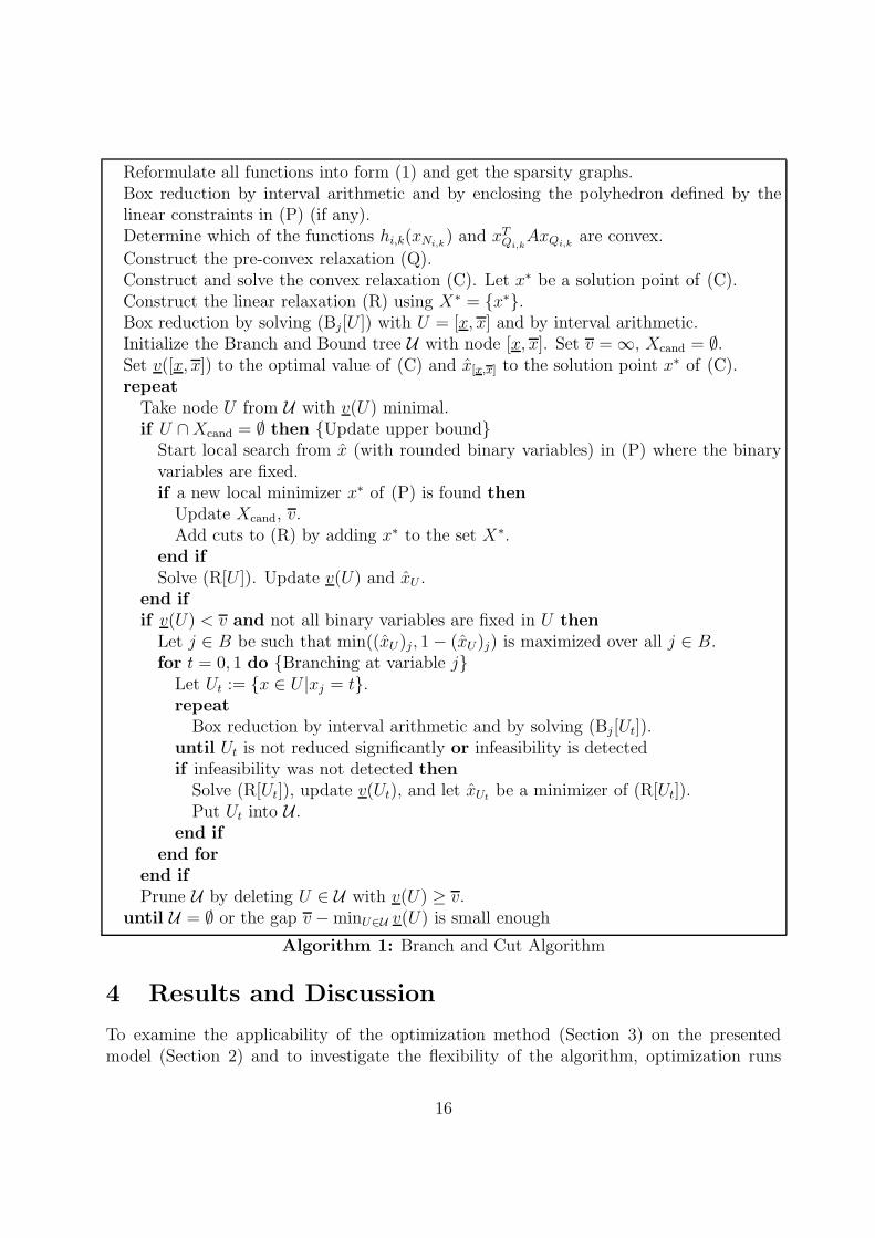
Reformulate all functions into form (1) and get the sparsity graphs.Box reduction by interval arithmetic and by enclosing the polyhedron defined by thelinear constraints in (P) (if any).Determine which of the functions hi,k(xNi,k

) and xTQi,k

AxQi,kare convex.

Construct the pre-convex relaxation (Q).Construct and solve the convex relaxation (C). Let x∗ be a solution point of (C).Construct the linear relaxation (R) using X∗ = {x∗}.Box reduction by solving (Bj[U ]) with U = [x, x] and by interval arithmetic.Initialize the Branch and Bound tree U with node [x, x]. Set v = ∞, Xcand = ∅.Set v([x, x]) to the optimal value of (C) and x[x,x] to the solution point x∗ of (C).repeat

Take node U from U with v(U) minimal.if U ∩ Xcand = ∅ then {Update upper bound}

Start local search from x (with rounded binary variables) in (P) where the binaryvariables are fixed.if a new local minimizer x∗ of (P) is found then

Update Xcand, v.Add cuts to (R) by adding x∗ to the set X∗.

end ifSolve (R[U ]). Update v(U) and xU .

end ifif v(U) < v and not all binary variables are fixed in U then

Let j ∈ B be such that min((xU)j, 1 − (xU)j) is maximized over all j ∈ B.for t = 0, 1 do {Branching at variable j}

Let Ut := {x ∈ U |xj = t}.repeat

Box reduction by interval arithmetic and by solving (Bj [Ut]).until Ut is not reduced significantly or infeasibility is detectedif infeasibility was not detected then

Solve (R[Ut]), update v(Ut), and let xUtbe a minimizer of (R[Ut]).

Put Ut into U .end if

end forend ifPrune U by deleting U ∈ U with v(U) ≥ v.

until U = ∅ or the gap v − minU∈U v(U) is small enough

Algorithm 1: Branch and Cut Algorithm

4 Results and Discussion

To examine the applicability of the optimization method (Section 3) on the presentedmodel (Section 2) and to investigate the flexibility of the algorithm, optimization runs

16

for four different cases of electric power and process steam demand were performed. Theobjective was to find a design of the cogeneration plant with minimum levelized total coststhat fulfills the specified requirements.

Due to the complexity of the model, a preprocessing has to be applied for the localoptimization step of the algorithm. In the preprocessing, the model is split up and initially,a part of it is solved. In the second step, the result of the first step is taken into accountto compute a locally optimal solution for the complete model. For an optimization run,30000 iterations of the Branch-and-Bound algorithm were performed. Within LaGO, theLPs are solved by CPLEX 9.0 [14] and the local search is done by CONOPT 3.14P [12].

In the discussion of the results, no values of the 76 decision variables are presentedfor reasons of simplicity. Instead, the structure of the resulting cogeneration plant forthe respective case is explained briefly. In addition, the most important parameters arepresented in Table 2: total electric power output Wtotal, thermal efficiency ηth (representingthe sum of electric and thermal output in relation to the fuel input), and total levelizedcosts TRRlev (representing the levelized hourly cost of the plant throughout its lifetime).The efficiency values are based on the lower heating value of the fuel.

4.1 Case 1: single electric power output of 300 MW

In the first case, a design for pure power generation with a capacity of 300 MW is stud-ied. This case represents a relatively simple case because no process steam extractionhas to be considered and the power demand is in the middle of the capacity range of thesuperstructure. The design produced by LaGO consists of a simple gas turbine withoutintercooling, air preheater, or sequential combustion. The bottoming cycle is designedas a two-pressure-level process with reheating after the high-pressure part of the steamturbine. The characteristic parameters of the design can be found in the first column ofTable 2. The thermal efficiency of almost 57% is in line with the efficiencies of existingcombined-cycle power plants at this capacity range. Since electricity is the only product ofthe plant, the levelized total cost of 12674 €/h can easily be converted into the levelizedcost of electricity (for 8000 hours of yearly operation) and results in a value of about 4.2Eurocent/kWh. Compared to the electricity costs of today’s combined-cycle power plantsand taking the future escalation of the fuel price into account, these results are realistic.

4.2 Case 2: single electric power output of 400 MW

For the second case, the required electric power output of 400 MW reaches the upperbound of the capacity of the superstructure. Looking at characteristic parameters in thesecond column of Table 2, it can be seen that the thermal efficiency almost reaches 59%,which corresponds to the thermal efficiency of today’s large-scale combined-cycle powerplants. The design consists of a simple gas turbine as topping cycle and a three-pressurelevel steam cycle including a reheater as bottoming cycle. The more complex structure ofthe steam cycle leads to an increased efficiency compared to the first case. The costs of

17

electricity amount again to about 4.2 Eurocent/kWh. As in the first case, the gas turbinegenerates around two-thirds of the total electric power output.

4.3 Case 3: electric power output of 90 MW and process steamextraction of 99.5 t/h

The third case introduces process steam extraction into the design. The specifications of90 MW electric power generation and process steam extraction of 99.5 t/h at a pressurelevel of 4.5 bar represent the demand of an existing paper factory. The design of thecogeneration plant consists of a simple gas turbine and a two-pressure steam cycle. Here, areheating of the medium-pressure steam is not implemented resulting in a lower efficiencyof the steam cycle. Compared to the first and second cases, the percentage of electricpower contributed by the steam cycle is much lower which is a result of the high amountof steam extracted from the steam cycle. Since steam can be produced with a much higherenergetic efficiency than electricity, the overall thermal efficiency of the design outperformsclearly the cases with pure electric power generation.

4.4 Case 4: electric power output of 290 MW and process steam

extraction of 150 t/h at different pressure levels

The fourth case represents again a cogeneration plant but with maximum exploitation ofthe complexity of the superstructure. Therefore, process steam extraction at three differentpressure levels (40 t/h at 50 bar, 40 t/h at 15 bar, and 70 t/h at 3.5 bar) and an electricpower output of 290 MW is required. The resulting design consists of a simple gas turbineand a three-pressure-level steam cycle including a reheater. The power-to-steam ratio ishigher than in the third case which results in a lower overall thermal efficiency but in amore complex structure of the steam cycle.

Table 2: Results from the cases considered in the optimization of the superstructure fordifferent demands for electric power and process steam.

Case 1 Case 2 Case 3 Case 4

Wtotal [MW] 300 400 90 290ηth [%] 56.72 58.59 77.19 68.45TRRlev [€/h] 12674 16771 5022 13424

4.5 Sensitivity Analysis

A sensitivity analysis examines the influence of certain parameters, which are usually keptconstant during an optimization run, on the result of the optimization. These parameters

18

describe technical limits of plant components or are estimates of uncertain future economicdevelopments. Knowledge of the effects of such parameters on the resulting design and onthe associated costs is very valuable for the design engineer. Among the many possibleparameters, the effect of the fuel price, the rate of increase of the fuel price, and the numberof planned operating hours are chosen to demonstrate the sensitivity analysis performedwith LaGO.

For the base case 1, the price of natural gas is set to 4 €/GJ. In the sensitivity analysisthis price is changed to 3.5 €/GJ (representing a lower limit), and to 4.5 €/GJ (represent-ing a higher limit). The specified capacity for the power plant remains equal to 300 MW.To examine the influence of the fuel price, optimization runs with fuel prices of 3.5 €/GJ,4 €/GJ, and 4.5 €/GJ are performed. The levelized total costs of the three resulting de-signs are then calculated with the three different values of the fuel price and are shown inTable 3. For example, the levelized total costs displayed in line 1 of column 3 of this tableresult from a design which was optimized for a fuel price of 4.5 €/GJ but here is calculatedwith a fuel price of 3.5 €/GJ. If the fuel price would have a noticeable influence on theoptimization, the design which is calculated with the fuel price for which it is optimizedshould always yield the lowest costs.

In Table 3, noticeable differences in costs can only be seen between the optimizationruns for a fuel price of 3.5 €/GJ and a fuel price of 4.5 €/GJ. For a fuel price of 3.5 €/GJ,the levelized costs for the plant which is optimized for this fuel price are 25 €/h less thanif it is optimized for 4.5 €/GJ. In contrast, for a fuel price of 4.5 €/GJ, the levelizedcosts of the plant are 27 €/GJ less if it is optimized for this price compared to the designoptimized for 3.5 €/GJ. Thus, the value of the fuel price clearly influences the resultingdesign of the cogeneration plant.

Table 3: Effect of the fuel price on the resulting designs showing the TRRlev in €/h

Values calcu- Design optimized forlated with 3.5 €/GJ 4.0 €/GJ 4.5 €/GJ3.5 €/GJ 11436 11441 114614.0 €/GJ 12678 12674 126774.5 €/GJ 13921 13907 13894

To analyse the effect of the rate of increase of the fuel price, the same investigation isperformed. In addition to the base rate of 1.0%, the values of 0.5% and 1.5% are considered.Table 4 shows the results of the calculations. Looking at the values of the levelized totalcosts no noticeable tendency can be observed. Taking into account the large percentageof variation for this parameter during the analysis, it can be concluded that the rate ofincrease of the fuel price has no significant influence on the optimization.

The last parameter under investigation is the average number of annual operating hoursthe plant is designed for. They are varied between 8000, 7000, 5000, and 4000 hours. Theresults are presented in Table 5. It can be seen that the design which is calculated with the

19

Table 4: Effect of the rate of increase of the fuel price on the resulting designs showing theTRRlev in €/h

Values calcu- Design optimized forlated with 0.5% 1.0% 1.5 %0.5 % 12290 12296 122871.0 % 12667 12674 126611.5 % 13467 13477 13455

number of operation hours for which it is optimized always yields the lowest cost. Moreover,the greater the difference to the number of hours the plant is optimized for becomes, thehigher the total levelized costs are. Here, the influence of the yearly operation hours onthe optimization results is clearly evident.

Table 5: Effect of the number of annual operation hours on the resulting designs showingthe TRRlev in €/h

Values calcu- Design optimized forlated with 4000 h 5000 h 7000 h 8000 h4000 h 15233 15253 15368 154395000 h 14268 14248 14292 143337000 h 13167 13101 13062 130698000 h 12823 12742 12668 12664

4.6 Discussion

The various optimizations performed with LaGO produce reasonable results in all cases.The thermal efficiencies and the levelized total costs of the resulting designs are within therange of existing combined-cycle power plants of the corresponding capacity. This provesthe applicability and functionality of LaGO as well as the plausibility of the model of thesuperstructure. The sensitivity analysis also produces reasonable and useful results andshows the flexibility of the optimization algorithm.

From the energy engineering point of view the results allow some interpretations inregard to the design of combined-cycle power plants. All investigated cases show a greatunity in the gas turbine design which goes in line with the structure of industrial heavyduty gas turbines installed in large commercial CCPPs. The gas turbine system is alwaysa simple cycle with a pressure ratio of around 18. Differences between the several casescan mainly be found in the steam cycle design. For electricity generation only, the fuelsavings due to the efficiency increase outweigh the investment costs in additional or moreefficient plant components and result in a greater complexity of the steam cycle. In the

20

case of significant process steam extraction, the complexity of the steam cycle is not acrucial factor anymore and leads to simpler designs.

5 Conclusions

A superstructure of a combined-cycle-based cogeneration plant was developed and opti-mized. The model allows the simultaneous optimization of the operational parametersand the structure of the plant. The resulting nonconvex mixed-integer nonlinear problem(MINLP) is solved by LaGO. The solver generates a convex relaxation of the MINLP andapplies a Branch and Cut algorithm to the convex relaxation.

Various optimization runs with different requirements for the electric power and processsteam demand as well as sensitivity analyses for different parameters were performed. Theoptimization tool produces reasonable results for all cases which proves its applicabilityand functionality.

Regarding the design of combined-cycle-based cogeneration plants, the results showthat the focus should be set on the configuration of the steam cycle. Moreover, the optionof process steam extraction has to be taken into account and decides over the complexity ofthe design. The fact that only fixed gas turbine systems are available on the market is nota disadvantage because all designs obtained contain the same simple gas turbine process.

Acknowledgements: This work was supported by the German Science Foundation(DFG) under grants NO 421/2-1, TS 79/1-1, and TS 79/1-3.

References

[1] C. S. Adjiman, S. Dallwig, C. A. Floudas, and A. Neumaier. A global optimization method,αBB, for general twice-differentiable constrained NLPs — I. Theoretical advances. Comput-

ers & Chemical Engineering, 22:1137–1158, 1998.

[2] C. S. Adjiman and C. A. Floudas. Rigorous convex underestimators for general twice-differentiable problems. Journal of Global Optimization, 9:23–40, 1996.

[3] T. Ahadi-Oskui. Optimierung des Entwurfs komplexer Energieumwandlungsanlagen. InFortschritt-Berichte, number 543 in Series 6. VDI-Verlag, Dusseldorf, Germany, 2006.

[4] T. Ahadi-Oskui and G. Tsatsaronis. Optimization of the design of complex energy conversionsystems using mathematical programming and genetic algorithms. In Proceedings of the

ASME International Mechanical Engineering Congress and Exposition, Chicago, November2006. IMECE2006-14344.

[5] A. Bejan, G. Tsatsaronis, and M. Moran. Thermal Design and Optimization. John Wiley &Sons, Inc., New York, 1996.

21

[6] P. Belotti, J. Lee, L. Liberti, F. Margot, and A. Wachter. Branching and bounds tighteningtechniques for non-convex MINLP. Optimization Methods and Software, 24(4-5):597–634,2009.

[7] F. Cziesla, G. Tsatsaronis, and Z. Gao. Avoidable thermodynamic inefficiencies and costsin an externally-fired combined-cycle power plant. Energy – The International Journal,31:1472–1489, 2006.

[8] D. Dressler. Kostenabschatzung von ausgewahlten Kraftwerkskomponenten. Studienarbeit,Institut fur Energietechnik, TU Berlin, 1994.

[9] M. A. Duran and I. E. Grossmann. An outer-approximation algorithm for a class of mixed-integer nonlinear programs. Mathematical Programming, 36:307–339, 1986.

[10] M. D. Duran, A. Rovira de Antonio, and M. Valdes. The Application of Genetic Algorithmsfor the Thermoeconomic Optimization of Combined Cycle Gas Turbine Power Plants. InECOS 2004, Proceedings of the 17th Conference on Energy-Efficient, Cost-Effective, and

Environmentally-Sustainable Systems and Processes, pages 1421–1432. Instituteo Mexicanodel Petroleo, 2004.

[11] R. Fletcher and S. Leyffer. Solving mixed integer nonlinear programs by outer approximation.Mathematical Programming, 66(3(A)):327–349, 1994.

[12] GAMS Development Corp. GAMS - The Solver Manuals. Washington DC, 2003.

[13] Gas turbine world handbook. Pequot Publishing Inc., 1997.

[14] IBM. CPLEX. http://www-01.ibm.com/software/integration/optimization/cplex.

[15] M. Judes. MINLP-Optimierung des Entwurfs und des stationaren Betriebs von Kraftwerkenmit mehreren Arbeitspunkten. In Fortschritt-Berichte, number 579 in Series 6. VDI-Verlag,Dusseldorf, Germany, 2009.

[16] M. Judes, A. Christidis, C. Koch, L. Pottel, and G. Tsatsaronis. Combined optimizationof the operation of existing power plants with the design and operation of heat storagesystems for a large district heating network. In S. Nebra, S. de Oliveira Jr, and E. Bazzo,editors, Proceedings of the 22nd International Conference on Efficiency, Costs, Optimization,

Simulation and Environmental Impact of Energy Systems, ECOS, pages 291–300, Foz doIguacu, Brazil, 2009.

[17] M. Judes, G. Tsatsaronis, and S. Vigerske. Optimization of the design and partial-load oper-ation of power plants using mixed-integer nonlinear programming. In J. Kallrath, P. Parda-los, S. Rebennack, and M. Scheidt, editors, Optimization in the Energy Industry, chapter 9.Springer, 2009.

[18] R. Kehlhofer, B. Rukes, F. Hannemann, and F. Stirnimann. Combined-Cycle Gas and Steam

Turbine Power Plants. PennWell, third edition, 2009.

[19] O. Knacke, O. Kubaschewski, and K. Hesselmann. Thermochemical Properties of Inorganic

Substances. Springer-Verlag, second edition, 1991.

22

[20] C. Koch, F. Cziesla, and G. Tsatsaronis. Optimization of combined cycle power plants usingevolutionary algorithms. Chemical Engineering and Processing, 46:1151–1159, 2007.

[21] S. Leyffer. Integrating SQP and branch-and-bound for mixed integer nonlinear programming.Computational Optimization and Applications, 18:295–309, 2001.

[22] A. Neumaier. Complete search in continuous global optimization and constraint satisfaction.In Acta Numerica, volume 13, chapter 4, pages 271–370. Cambridge University Press, 2004.

[23] I. Nowak. Relaxation and Decomposition Methods for Mixed Integer Nonlinear Programming.Birkhauser, 2005.

[24] I. Nowak and S. Vigerske. LaGO: a (heuristic) branch and cut algorithm for nonconvexMINLPs. Central European Journal of Operations Research, 16(2):127–138, 2008. preprintavailable at http://www.mathematik.hu-berlin.de/publ/pre/2006/P-06-24.ps.

[25] I. Quesada and I. E. Grossmann. An LP/NLP based branch and bound algorithm for convexMINLP optimization problems. Computers & Chemical Engineering, 16:937–947, 1992.

[26] R. Romero, A. Zobaa, E. Asada, and W. Freitas. Mathematical optimisation techniquesapplied to power systems operation and planning. International Journal of energy technology

and policy, 5(4):393–403, 2007.

[27] T. Savola. Simulation and Optimisation of Power Production in Biomass-Fuelled Small-ScaleCHP plants. Licentiate’s thesis, Helsinki University of Technology, March 2005.

[28] M. Tawarmalani and N. V. Sahinidis. Global optimization of mixed-integer nonlinear pro-grams: A theoretical and computational study. Mathematical Programming, 99:563–591,2004.

[29] M. Tawarmalani and N.V. Sahinidis. Convexification and Global Optimization in Continuous

and Mixed-Integer Nonlinear Programming: Theory, Algorithms, Software, and Applications.Kluwer Academic Publishers, 2002.

[30] G. Tsatsaronis, K. Kapanke, and A.M. Blanco Marigorta. Exergoeconomic estimates for anovel zero-emission process generating hydrogen and electric power. Energy – The Interna-

tional Journal, 33:321–330, 2008.

[31] R. Turton, R. C. Bailie, W. B. Whiting, and J. A. Shaeiwitz. Analysis, Synthesis and Design

of Chemical Processes. Prentice Hall, Upper Saddle River, 1998.

[32] W. Wagner and A. Kruse. Properties of Water and Steam - The Industrial Standard IAPWS-

IF97. Springer, 1998.

23