OPTIMIZING MARITIME CONTAINER TERMINAL OPERATIONS · GHENT UNIVERSITY FACULTY OF ECONOMICS AND...
126
GHENT UNIVERSITY FACULTY OF ECONOMICS AND BUSINESS ADMINISTRATION ACADEMIC YEAR 2010-2011 OPTIMIZING MARITIME CONTAINER TERMINAL OPERATIONS Master Thesis nominated to obtain the degree of Master of Business Economics: Business Engineering Bart Gadeyne and Pieter Verhamme under the leadership of Prof. dr. ir. Birger Raa
Transcript of OPTIMIZING MARITIME CONTAINER TERMINAL OPERATIONS · GHENT UNIVERSITY FACULTY OF ECONOMICS AND...

GHENT UNIVERSITY
FACULTY OF ECONOMICS AND BUSINESS ADMINISTRATION
ACADEMIC YEAR 2010-2011
OPTIMIZING MARITIME CONTAINER TERMINAL
OPERATIONS
Master Thesis nominated to obtain the degree of
Master of Business Economics: Business Engineering
Bart Gadeyne and Pieter Verhamme
under the leadership of
Prof. dr. ir. Birger Raa

PERMISSION
The undersigned declare that the contents of this thesis may be consulted and / or reproduced,
provided that the source is acknowledged.
Bart Gadeyne
Pieter Verhamme

i
Abstract Never-ending growth in worldwide maritime container transportation automatically entails several
container terminal optimisation questions. In this master thesis, research on the topic of double
cycling in the quay crane scheduling problem (QCSP) is presented. Most papers concerning the QCSP
neglect several operational issues, such as sequence constraints and spreader setup times. As a
result, the related models lose grip with reality. This thesis clarifies important operational concerns
and presents a QCSP model that incorporates the main operational constraints. The proposed
heuristics are tested on real-life data and provide near-to-optimal solutions to the model within an
acceptable time period. The presented hybrid genetic algorithm yields the best results and shows
that double cycling can reduce vessel turn-around time by more or less 10%, depending on the given
stowage plan. The financial impact of this reduction in vessel completion time is estimated in the last
chapter.
Keywords: double cycling; quay crane scheduling; terminal operations; genetic algorithm

ii
Preface Writing a thesis is not a piece of cake and certainly not when you have to write it together with your
best friend. Besides some occasional moments of frustration, we had great fun when elaborating this
master paper. However, with only having fun we would not have got very far. Hence we also would
like to thank a few people who inspired us.
First of all, we want to thank our promoter, Prof. Dr. Ir. B. Raa. Without him we could not have
started this work in the first place. He also pushed us in the right direction when needed.
Second, visiting the port of Antwerp and Zeebrugge brought us meaningful insights into the
fascinating world of shipping in general, and more specifically into maritime container
transportation. Therefore we would also like to thank Rowan Van Schaeren for the tour in the port of
Antwerp and for supplying a number of important ideas and work items. Furthermore, we would like
to express our gratitude to Philippe Wyngaert for the insightful roundtrip in the port of Zeebrugge
and all provided information and documentation. Without him, it would not have been possible to
understand several operational issues. We also want to thank the container terminal operator PSA
Antwerp for their cooperation and for providing the necessary data for this master paper.
In addition, many thanks go to Vincent Van Peteghem for his insights and suggestions regarding
useful heuristic solution methods.
We would also like to express our sincere thanks to Nathalie Demeyer and Mark Van Landschoot for
reading through and correcting this thesis.
Last but not least, we would like to acknowledge the role of our parents, family and friends for being
a constant source of support and strength. We warmly appreciate their contribution.

iii
Table of contents Abstract .................................................................................................................................................... i
Preface ......................................................................................................................................................ii
Table of contents ..................................................................................................................................... iii
List of figures ........................................................................................................................................... vi
List of tables .......................................................................................................................................... viii
Chapter 1. Introduction ..................................................................................................................... 1
1.1. Background .............................................................................................................................. 1
1.2. Structure of this paper ............................................................................................................ 2
Chapter 2. Container handling at terminals – description ................................................................ 4
2.1. Container types ....................................................................................................................... 4
2.2. Vessel layout ............................................................................................................................ 5
2.3. Container terminal – Interfaces and handling equipment ...................................................... 7
2.4. Container lifting system .......................................................................................................... 8
2.5. Loading and unloading ............................................................................................................ 9
2.5.1. Loading of a vessel ......................................................................................................... 10
2.5.2. Unloading of a vessel ..................................................................................................... 10
2.5.3. Alternating loading and unloading ................................................................................ 11
2.6. Problem definition ................................................................................................................. 12
Chapter 3. Literature review ........................................................................................................... 14
3.1. Container handling ................................................................................................................ 14
3.1.1. Container types ............................................................................................................. 14
3.1.2. Container sequencing problem ..................................................................................... 14
3.1.3. Container reshuffling ..................................................................................................... 15
3.2. Container stowage ................................................................................................................ 15
3.3. Berth and crane allocation .................................................................................................... 18
3.3.1. Berth Allocation ............................................................................................................. 18
3.3.2. Crane Allocation ............................................................................................................ 19
3.3.3. Crane Scheduling ........................................................................................................... 20
3.4. Quay crane efficiency ............................................................................................................ 21
3.5. Other operational aspects ..................................................................................................... 24
Chapter 4. Model design ................................................................................................................. 26
4.1. Characteristics ....................................................................................................................... 26
4.1.1. Travelling Salesman Problem ........................................................................................ 26

iv
4.1.2. Vehicle Routing Problem and PickUp and Delivery Problems ....................................... 27
4.1.3. Parallel Machine Scheduling Problem with Sequence-Dependent Setup Times .......... 28
4.1.4. NP-hardness .................................................................................................................. 29
4.2. Assumptions .......................................................................................................................... 29
4.3. A first model .......................................................................................................................... 31
4.3.1. Modelling approach ...................................................................................................... 31
4.3.2. Mathematical formulation ............................................................................................ 31
4.3.3. The interference constraint ........................................................................................... 35
4.4. A second model ..................................................................................................................... 36
4.4.1. Modelling approach ...................................................................................................... 36
4.4.2. Solution representation................................................................................................. 38
4.4.3. Mathematical formulation ............................................................................................ 41
4.4.4. Constraint examples ...................................................................................................... 45
4.5. Small comparison between both models .............................................................................. 48
Chapter 5. Solution methodology ................................................................................................... 50
5.1. Input ...................................................................................................................................... 50
5.2. Preprocessing ........................................................................................................................ 52
5.3. Heuristics ............................................................................................................................... 53
5.3.1. Current way of working ................................................................................................. 53
5.3.2. Greedy heuristic ............................................................................................................ 56
5.3.3. GRASP ............................................................................................................................ 58
5.3.4. Intelligent constructive heuristic ................................................................................... 60
5.3.5. Local search improvement heuristics ............................................................................ 63
5.3.6. Intelligent constructive heuristic with randomized extension ...................................... 63
5.3.7. Hybrid genetic algorithm ............................................................................................... 65
5.3.8. Intermediate solution .................................................................................................... 72
5.3.9. Container crane assignment methodology ................................................................... 74
5.4. Results ................................................................................................................................... 75
Chapter 6. Sensitivity analysis ......................................................................................................... 79
Chapter 7. The economic point of view .......................................................................................... 80
7.1. Financial impact ..................................................................................................................... 80
7.2. Implementation issues .......................................................................................................... 82
7.2.1. Diffusion of benefits ...................................................................................................... 82
7.2.2. Crane operator productivity .......................................................................................... 83

v
Chapter 8. Conclusion and recommendations ................................................................................ 84
8.1. General conclusion ................................................................................................................ 84
8.2. Recommendations for further research ................................................................................ 85
Chapter 9. References ..................................................................................................................... 86
Chapter 10. Annexes ......................................................................................................................... 91
10.1. Container type descriptions .................................................................................................. 91
10.2. Container size type codes according to ISO 6346 ................................................................. 93
10.3. Bromma STS45E Twin-Lift All-Electric ................................................................................... 95
10.4. Semi-automatic twistlock example ....................................................................................... 96
10.5. Solution representation example with one QC ..................................................................... 97
10.6. The current way of working heuristic used to solve the sequence of bay1 .......................... 98
10.7. Output for bay 1 with greedy heuristic ............................................................................... 101
10.8. Output intelligent constructive heuristic ............................................................................ 105
10.9. Output hybrid GA ................................................................................................................ 108

vi
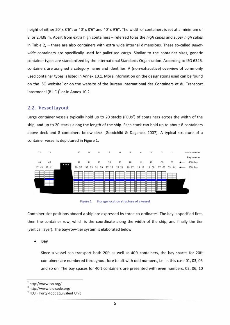
List of figures Figure 1 Storage location structure of a vessel ................................................................................. 5
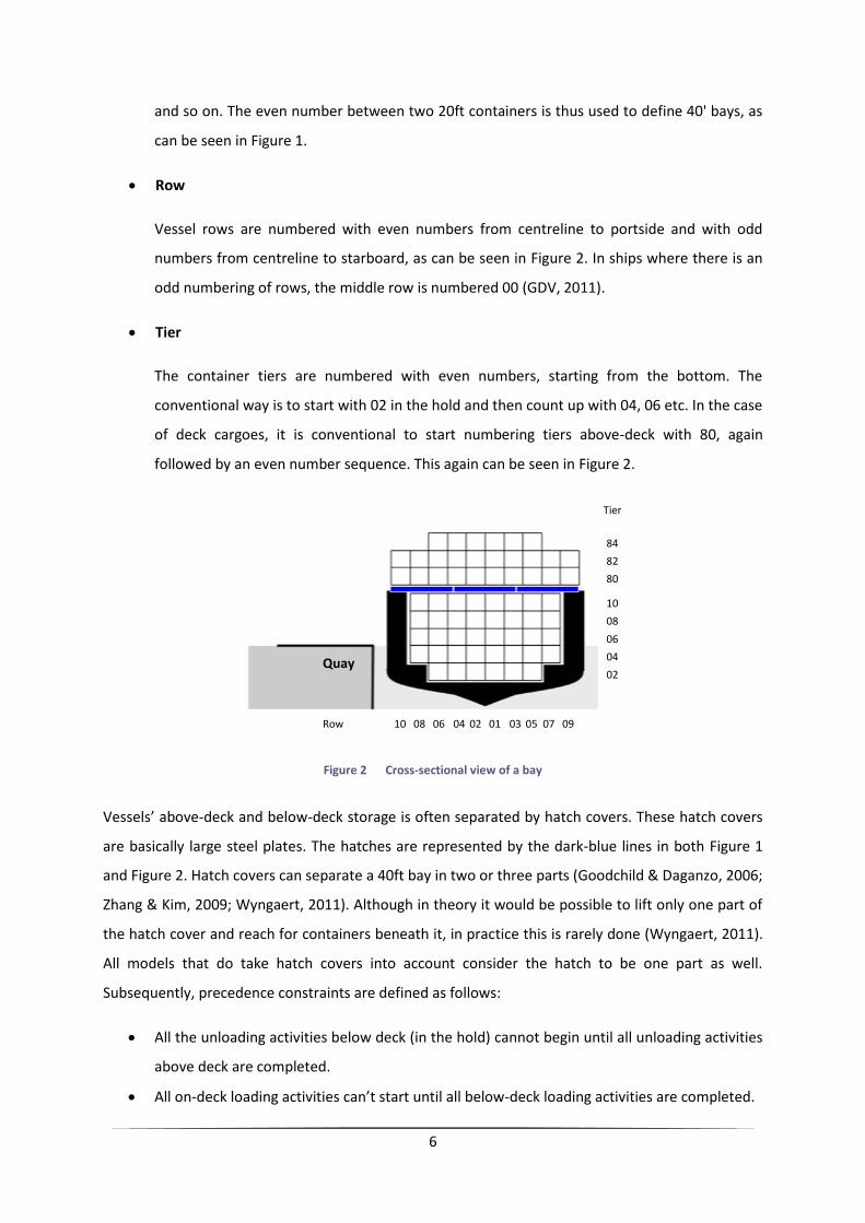
Figure 2 Cross-sectional view of a bay .............................................................................................. 6
Figure 3 Simple example of general stack positions ......................................................................... 7
Figure 4 Schematic view of a container terminal .............................................................................. 7
Figure 5 The usage of flipper guides during container pick-up ......................................................... 9
Figure 6 (a) Loading and (b) Unloading of a container .................................................................... 10
Figure 7 Stability of a ship. (a) metacentric height (GM) and heel, (b) trim. .................................. 17
Figure 8 Single and twin lift (a) single-lift of 40ft container (b) single-lift of 20ft container
(c) twin-lift of two 20 ft containers ................................................................................... 22
Figure 9 Tandem-lift (a) two 40ft containers (b) four 20ft containers ............................................ 22
Figure 10 (a) Unloading using single cycling (b) Unloading and loading with double cycling ........... 23
Figure 11 (a) Landside operations when single cycling (b) double cycling........................................ 24
Figure 12 Interference constraint example ....................................................................................... 35
Figure 13 An easy QCSP example ...................................................................................................... 38
Figure 14 Solution representation of the easy QCSP example (Information duplication per QC) .... 39
Figure 15 Solution representation of the easy QCSP example (Information duplication per bay) ... 40
Figure 16 Examples on the non-preemption constraint ................................................................... 46
Figure 17 Examples on single and double cycling rules .................................................................... 47
Figure 18 Sample of a BAPLIE file ...................................................................................................... 51
Figure 19 Sample of EdiRite presentation of a BAPLIE file ................................................................ 51
Figure 20 Output of the current way of working heuristic ............................................................... 55
Figure 21 A sample of the construction list of the previously generated container sequence
of bay 1 .............................................................................................................................. 55
Figure 22 Output when using the greedy heuristic ........................................................................... 57
Figure 23 GRASP variant .................................................................................................................... 59
Figure 24 Result of variant on GRASP ................................................................................................ 60
Figure 25 The possible solution structures for a bay ........................................................................ 61
Figure 26 Sample of output of intelligent constructive heuristic ...................................................... 62
Figure 27 Insertion mutation operator ............................................................................................. 66
Figure 28 The methodology of the hybrid genetic algorithm ........................................................... 68
Figure 29 Example of the recombination method (length = 5; index = 0) ........................................ 68
Figure 30 PPX crossover operator (Hui, Dong, & Guanghong, 2008) ................................................ 69
Figure 31 The four examined mutation methods ............................................................................. 70

vii
Figure 32 Evolution between solution of constructive heuristic with randomized extension
and solution of hybrid genetic........................................................................................... 72
Figure 33 Time loss due to distance between containers in dual loop ............................................. 73
Figure 34 Intermediate result for bay 1 ............................................................................................ 73
Figure 35 Result for three quay cranes when using the intelligent constructive heuristic and
local search heuristics ....................................................................................................... 75
Figure 36 Relationship between the number of samerows and CPU time per container ................ 76
Figure 37 Effect of the number of containers per bay on the CPU time ........................................... 77
Figure 38 The relation between the number of containers per vessel and the required CPU time
(for hybrid genetic) ............................................................................................................ 78
Figure 39 Time gain when there is no setup time between containers of the same bay ................. 79

viii
List of tables Table 1 Possible container lengths ....................................................................................................... 4
Table 2 Possible container heights ....................................................................................................... 4
Table 3 Possible combinations of variables for constraint (8) on a certain moment m .................... 34
Table 4 Initial situation for the interference constraint example ...................................................... 36
Table 5 Interference situation for the interference constraint example ........................................... 36
Table 6 Time units per QC action ....................................................................................................... 37
Table 7 Results of the examples on the non-preemption constraint ................................................ 46
Table 8 Results of the examples on the single cycling and double cycling rules ............................... 48
Table 9 Comparison between Model 1 and Model 2 ......................................................................... 49
Table 10 Comparison of results........................................................................................................ 64
Table 11 Test result for four mutations (average improvements per bay are displayed) ............... 70
Table 12 Test results for most promising mutations ....................................................................... 71
Table 13 The average improvement over the extended constructive heuristic for the hybrid
genetic algorithm with and without mutations ................................................................ 71
Table 14 Efficiency gains for different datasets ............................................................................... 75
Table 15 Extra revenues and costs from double cycling .................................................................. 80

1
Chapter 1.
Introduction
1.1. Background
Today, ports are facing a considerable growth in worldwide container transportation, automatically
entailing several optimisation questions. Transhipment in northern Europe is forecasted to almost
triple between 2001 and 2015, from 6.72 mio TEU1 to 17.1 mio TEU (Baird, 2006). Because of
economies of scale, container vessels are also increasing in size, capable of carrying from 8.000 TEU
in 2001 (Meersmans & Dekker, 2001) up to 14.770 TEU in 2011 (Maersk Line, 2011). In short, ports
have to deal with both more as well as bigger container vessels. With respect to this evolution,
container terminals are assigned an increasingly important role as key hubs within the overall
transportation network.
Important factors for a container terminal are the efficiency of stacking and transport of this large
number of containers to and from the ship (Stahlbock & Voß, 2008). An accompanying and perhaps
more crucial factor to container terminals is the vessels’ turn-around time, since this is a key issue in
terms of the port’s competitiveness (Tongzon & Heng, 2005). There are several practical explanations
for this:
Large vessels tend to call at several ports in a multiport itinerary (Baird, 2006). Consequently,
retardation in one of the ports within the itinerary will cause a delay for the next ports.
In addition, berth allocation possibilities for ports are limited. During peak periods this might
cause vessels having to wait if turn-around times are rather high. Obviously, this is an
undesirable situation, and moreover, terminals can’t fully control the inflow of vessels in the
port.
The explanations stated above are of course interrelated. On one hand, waiting in one port will cause
delays for the next port. On the other hand, the incurred delays could also cause additional waiting
time in the next port, just because the vessel did not berth at the anticipated point of time. In short,
from the viewpoint of the customer – who wants to have their containers delivered on time – it is
important that the vessel turnaround and waiting time at ports is minimized because this turns out
to be an expensive activity (Tongzon & Heng, 2005).
1 TEU = Twenty-Foot Equivalent Unit

2
Indeed, the overall efficiency of a ship is closely related to the total time spent on a voyage, and
hence to the ship’s time at ports. Therefore, the economies of scale of large vessels is to a large
extent depending on the port’s productivity and efficiency (Cullinane & Khanna, 1999). The fact that
the economies of scale of larger vessels can only be realized if the handling speed at the harbours
increases accordingly, is stated by Meersmans and Dekker (2001) as well.
This brings us to the subject of this paper in which we want to investigate the key bottleneck to port
productivity: quay crane efficiency (Li & Huo, 2005; Goodchild & Daganzo, 2006). Quay cranes are the
most expensive single unit of handling equipment in port container terminals (5–10 million dollars
per quay crane). Because of this, one of the key operational bottlenecks at ports is quay crane
availability (Crainic & Kim, 2007a.). By improving quay crane efficiency, ports can reduce ship turn-
around time and improve port productivity, to ensure that the economic advantages of large vessels
are not cancelled out by long port stay times. In contrast to increasing capacity by terminal expansion
or the acquisition of extra handling equipment, we will investigate the effects of applying double-
cycling strategies as a low-cost method to increase capacity.
For a comprehensive overview of most of the operational research problems in container terminals,
we refer to the surveys of Meersmans and Dekker (2001), Vis and de Koster (2003) and Stahlbock
and Voß (2008).
1.2. Structure of this paper
In the next chapter, a brief but fairly complete overview of basic container handling elements and
activities is given. This overview is based on publicly available papers and our visit to the Port of
Antwerp and the Port of Zeebrugge. This chapter provides information on both containers, container
vessels, as well as container terminals and (un)loading practices. In addition, the problem definition
of this paper is stated at the end of Chapter 2.
While Chapter 2 mainly focuses on practical operational concerns, Chapter 3 mainly provides the
theoretical background, by giving an overview of literature on operational research problems. Both
container loading and unloading practices are discussed as well during this chapter, as well as the
berth and quay crane allocation problem. Furthermore quay crane scheduling and crane efficiency
will be reviewed along with some other smaller operational aspects.
Afterwards two mixed integer linear problem models are proposed in Chapter 4. The characteristics
of the problem will be discussed, as well as the assumptions made. Eventually, two models are
presented and elaborated into detail. Finally, a small comparison is made between both models.

3
Next to that the practical implementation of the problem instance is described in Chapter 5, together
with the implemented heuristics. In this chapter, a greedy heuristic is presented, as well as a GRASP,
intelligent constructive and extended intelligent constructive heuristic. Finally, a hybrid genetic
algorithm is fully elaborated. The results of all heuristic methods mentioned above are compared to
the current way of handling containers and an intermediate solution. The quay crane assignment
method is briefly discussed as well, after which general results of the implemented solution methods
are presented, based on 5 different data sets.
Next, in Chapter 6 a sensitivity analysis is conducted, while Chapter 7 reviews the problem from an
economic point of view. Finally, a conclusion is drawn in Chapter 8 with some recommendations for
further research.

4
Chapter 2.
Container handling at terminals – description
2.1. Container types
Since its introduction in the sixties, the container has rapidly taken over the market of
intercontinental transport (Meersmans & Dekker, 2001). Basically, containers can be described as
being large boxes, used to transport goods from one destination to another. Compared to
conventional bulk, the use of containers has several advantages, including less product packaging,
less product damage and higher productivity.
Nowadays, dimensions of ‘general purpose freight containers’ have been standardised by the
International Standards Organization (ISO). This standardisation enables a uniform container
handling, entailing large savings of time and money. The possible container lengths are listed below
in Table 1. The possible container heights are listed in Table 2 (Algemene Handleiding Bediende
Containerterminals - Versie 5.3, 2011). Notice that these are the (minimum) external dimensions of
containers.
Length (ft) Length (m) Notation
10 3,048 10’
20 6,096 20’
30 9,144 30’
40 12,192 40’
45 13,716 45’
Table 1 Possible container lengths
Height (ft) Height (m) Remarks
4’6” 1,402 Also called ‘half-height’ container
8’ 2,438 Becomes less common
8’6” 2,621 Most common height
9’ 2,743 Uncommon and only for 20’ containers
9’6” 2,926 High cubes, often used for 40’ containers
10’6” 3,231 Super high cubes
Table 2 Possible container heights
The 20 feet (20’) and 40 feet (40’) containers are most common in ocean transport. The most widely
used type of container is the general purpose (Dry Van) container, having an external length and
5
height of either 20’ x 8’6”, or 40’ x 8’6” and 40’ x 9’6”. The width of containers is set at a minimum of
8’ or 2,438 m. Apart from extra high containers – referred to as the high cubes and super high cubes
in Table 2, – there are also containers with extra wide internal dimensions. These so-called pallet-
wide containers are specifically used for palletised cargo. Similar to the container sizes, generic
container types are standardized by the International Standards Organization. According to ISO 6346,
containers are assigned a category name and identifier. A (non-exhaustive) overview of commonly
used container types is listed in Annex 10.1. More information on the designations used can be found
on the ISO website2 or on the website of the Bureau International des Containers et du Transport
Intermodal (B.I.C.)3 or in Annex 10.2.
2.2. Vessel layout
Large container vessels typically hold up to 20 stacks (FEUs4) of containers across the width of the
ship, and up to 20 stacks along the length of the ship. Each stack can hold up to about 8 containers
above deck and 8 containers below deck (Goodchild & Daganzo, 2007). A typical structure of a
container vessel is depictured in Figure 1.
Figure 1 Storage location structure of a vessel
Container slot positions aboard a ship are expressed by three co-ordinates. The bay is specified first,
then the container row, which is the coordinate along the width of the ship, and finally the tier
(vertical layer). The bay-row-tier system is elaborated below.
Bay
Since a vessel can transport both 20ft as well as 40ft containers, the bay spaces for 20ft
containers are numbered throughout fore to aft with odd numbers, i.e. in this case 01, 03, 05
and so on. The bay spaces for 40ft containers are presented with even numbers: 02, 06, 10
2 http://www.iso.org/
3 http://www.bic-code.org/
4 FEU = Forty-Foot Equivalent Unit
12 11 10 9 8 7 6 5 4 3 2 1 Hatch number
Bay number
46 42 38 34 30 26 22 18 14 10 06 02 40ft Bay
47 45 43 41 39 37 35 33 31 29 27 25 23 21 19 17 15 13 11 09 07 05 03 01 20ft Bay
6
and so on. The even number between two 20ft containers is thus used to define 40' bays, as
can be seen in Figure 1.
Row
Vessel rows are numbered with even numbers from centreline to portside and with odd
numbers from centreline to starboard, as can be seen in Figure 2. In ships where there is an
odd numbering of rows, the middle row is numbered 00 (GDV, 2011).
Tier
The container tiers are numbered with even numbers, starting from the bottom. The
conventional way is to start with 02 in the hold and then count up with 04, 06 etc. In the case
of deck cargoes, it is conventional to start numbering tiers above-deck with 80, again
followed by an even number sequence. This again can be seen in Figure 2.
Figure 2 Cross-sectional view of a bay
Vessels’ above-deck and below-deck storage is often separated by hatch covers. These hatch covers
are basically large steel plates. The hatches are represented by the dark-blue lines in both Figure 1
and Figure 2. Hatch covers can separate a 40ft bay in two or three parts (Goodchild & Daganzo, 2006;
Zhang & Kim, 2009; Wyngaert, 2011). Although in theory it would be possible to lift only one part of
the hatch cover and reach for containers beneath it, in practice this is rarely done (Wyngaert, 2011).
All models that do take hatch covers into account consider the hatch to be one part as well.
Subsequently, precedence constraints are defined as follows:
All the unloading activities below deck (in the hold) cannot begin until all unloading activities
above deck are completed.
All on-deck loading activities can’t start until all below-deck loading activities are completed.
Tier
84
82
80
10
08
06
04
02
Row 10 08 06 04 02 01 03 05 07 09
Quay

7
Hatches change the nature of the problem, because the stacks cannot be handled without
interruption. Below, a simple example is shown in Figure 3 to describe the characteristics of the
problem.
Figure 3 Simple example of general stack positions
Following the situation of hatch covers discussed above, we can describe some precedence constraints
according to the 3 hatches as follows:
In hatch 1: Unloading[A, B, C] Unloading [D, E] Loading [D, E] Loading [A, B, C]
In hatch 2: Unloading[F, G] Unloading [H, I] Loading [H, I] Loading [F, G]
In hatch 3: Unloading[J, K] Unloading [L, M, N] Loading [L, M, N] Loading [J, K]
The full elaboration of this example and a mathematical formulation on the problem of finding an
optimal loading and unloading sequence can be found in Zhang and Kim (2009).
2.3. Container terminal – Interfaces and handling equipment
Three basic areas can be distinguished within a container terminal: the berth area, the storage yard
area and the receipt/delivery area. From an operational point of view, we can also distinguish three
basic operations taking place in a container terminal: the seaside operations, the yard operations and
the landside operations (Vis & de Koster, 2003; Mastrogiannidou, 2008). A schematic view of a
container terminal is given by Figure 4 (Meersmans & Dekker, 2001):
Figure 4 Schematic view of a container terminal
A B C F G J K
Hatch
covers
D E H I L M N
Hatch 1 Hatch 2 Hatch 3

8
A container terminal is based on a maritime interface. In the berth area, quay cranes handle the
containers from large container vessels. They consist of an open lattice, with a beam extending over
the vessel. Quay cranes have a trolley and spreader which attach to the containers from the top,
which then are moved by cables. Two common types of QCs are used, namely rail mounted quay
cranes and rubber tire quay cranes.
Once a container has been moved from the ship, they are usually stacked in the container yard.
Different moving equipment can be used, such as trailers, automated guided vehicles (AGVs),
straddle carries (SCs), reach stackers, …. While reach stackers only handle empty containers (due to
weight restrictions), straddle carriers are capable of driving over a stack of loaded containers (3 or 4
containers high), lift it up and move it around. The main drawback of using trailers or AGVs is that
containers need to be handled a second time by stacking cranes to position them in or next to the
stack.
The stack in the yard is organized either into a block pattern, served by stacking cranes or into a
pattern of stacked rows of containers, enabling SCs to drive over these rows. In the USA on the other
hand, it is common to keep containers stored individually on the trailer, as there is often more space
available than in Europe and Asia. Empty containers are always stacked into a block pattern, since
reach stackers are not be able to drive over containers in order to pick them up.
Finally, as for the inland transportation, a container terminal can have different interfaces. There are
transfer points for trucks, as well as rail terminals, where containers are loaded onto or unloaded
from trains and possible barge service centers.
2.4. Container lifting system
As mentioned above, quay cranes use a spreader to pick up containers from the top. These spreaders
have a locking mechanism at each corner that attaches to the four corners of the container. More
information and key features of the Bromma ship-to-store STS45E twin-lift spreader can be found in
Annex 10.3. Similarly, spreaders are being used on straddle carriers to attach containers.
The locking system, called twist lock, consists of a male and female part. The female part is a
standardized corner casting, fitted to the container itself, whereas the male component is the actual
twist lock, fitted to the spreader. Likewise, stability of the container stacks on deck of the vessel is
ensured using the (semi-automatic) twist locks of the container below or the twist locks of the hatch
covers. A visual representation and example of using twist locks can be found in Annex 10.4.

9
Spreaders are often equipped with flipper guides that center the spreader on the container. The use
of flippers is explained in Figure 5. Additionally, these flipper guides can be used to speed up the
unloading process, which will be described in section 2.5.2.
Figure 5 The usage of flipper guides during container pick-up
A final thing to mention is that quay cranes are usually equipped with telescopic container spreaders,
able to adjust its length to lift 20ft, 40ft and 45ft containers. In addition, these spreaders can retract
to the 19’6” position in case it becomes jammed in the vessel’s 20ft cell.
2.5. Loading and unloading
During the handling of a container ship, the vessel-dispatcher is responsible for coordinating
container markers, crane operators, cargo inspectors, … Based on the vessel’s stowage plans, the
vessel dispatcher assigns cranes and SCs to the ship and provides them with automated planning-
and control systems. In all PSA Antwerp container terminals, all information entered by the container
markers and the SC drivers is processed by CTCS, the Container Terminal Control System. All other
systems, such as SPACE5 or SHIPS6, connected with CTCS, can appeal to the latest information, thanks
to one central database.
In practice, rules of thumb are applied to determine a sequence of container movements that
converts the arrival configuration of a bay into the departure configuration. Common rules are to
clear a bay by unloading containers tier wise or stack wise, starting at the quayside and ending at the
seaside of the vessel. When unloading is completed, export containers are loaded by reversing the
unloading pattern. (Meisel & Wichmann, 2010; Wyngaert, 2011). These practices are explained
below.
5 SPACE is an example of yard planning software, used for assigning the best possible stack position of a
5 container, within the container yard, as well as retrieving those containers.
6 SHIPS software is used to prepare for unloading and loading the vessel, as well as vessel planning software.
6 Based on resulting bayplans, SHIPS assists terminal workers in determining the optimal crane work scenario
6 with the best crane sequence

10
2.5.1. Loading of a vessel
The loading of a vessel starts with the straddle carriers picking up the export containers from the
container yard and delivering them to the apron. The SPACE yard planning software and yard
transport software, for instance TRAFIC (TRAnsporter Flow Control), is used to guide SC drivers the
specified stack position. This kind of software determines the most appropriate Move Instruction for
a SC.
Once a container has been delivered to the apron, the quay crane can start loading it onto the vessel,
in its predetermined container slot. As mentioned above, loading is often done in a tier wise order,
starting at the seaside of the vessel and ending at the quayside. This way, the previous placed
container can be used as a guidance to perfectly fit the container in place. The crane operator lets
the container slide against the previous one, and afterwards the container can almost immediately
be lowered and dropped to the right place. This whole concept is explained in Figure 6(a). After
having placed container 1, container 2 and 3 can be loaded quite easily right next to each other.
When finished with this tier, the next tier can be loaded similarly.
Figure 6 (a) Loading and (b) Unloading of a container
2.5.2. Unloading of a vessel
Unloading often happens by reversing the loading pattern, as can be seen in Figure 6(b). Thus,
unloading starts at the quayside and ends at the seaside of the vessel. Similarly to loading, the crane
operator now uses the spreader’s guidance flippers to slide against the container to be unloaded.
This way, the spreader is correctly positioned on top of the container after which the containers are
automatically locked on the spreader through the twist lock system. The quay crane can then deliver
the container to the apron.
(a) (b)

11
Depending on the type of container (empty, import, transit), the unloaded container is then moved
by a SC to a specific position in the container yard. Afterwards empty containers are stacked in a
block by reach stackers in order to save storage space.
2.5.3. Alternating loading and unloading
Usually, loading and unloading operations are temporarily decoupled (single cycling), which results in
an unproductive travel of the empty QC spreader in-between every two consecutive container moves
(Meisel & Wichmann, 2010). In contrast, by alternating loading and unloading operations (double
cycling), the number of empty movements of the QC spreader is reduced and the service of a bay is
accelerated. This concept is explained in Figure 10 (page 23).
Although the concept of double cycling might seem impeccable, double cycling entails quite a lot of
practical concerns that are often not described in scientific literature. For the (theoretical)
advantages of double cycling we refer to Section 3.4 (page 21). Practical restrictions are listed below,
based on both literature, as well as on the conversations with Wyngaert (2011):
First, although double cycling looks quite obvious, we must bear in mind that container handling
requires quite some human input. Even though large parts of, for instance, yard planning, stowage
planning and yard transport can be automated or IT-supported, container handling in essence
remains a complex cooperation of the vessel dispatcher, crane operators, SC drivers, cargo
inspectors, container markers, ... Consequently, all these people should receive training in the first
place, in order to pick up a new way of working. Additionally, this productivity gain entails an
increased workload and requires more concentration during work. Indeed, not only more containers
can be handled, but both import as well as export containers are mixed and handled simultaneously.
As a result, stress levels increase, leading to much more human errors compared to when using
single cycling.
Second, double cycling might require the use of additional handling equipment. Although double
cycling could lead to a reduction in the number of landside vehicles on the one hand (elaborated in
section 3.4 and Figure 11 on page 24), the QC productivity gain would result in a double need for
handling equipment according to Goodchild and Daganzo (2007). This would result in an additional
cost per container moved. Additionally, this situation would shift the bottleneck from the QC to the
landside operations, which is not desirable due to a risk of yard traffic congestions.
Third, in the current way of working, there is yet a software-related problem. Current software works
with two different modes, that is either the loading or unloading mode. Consequently, double cycling
would require continuous switching between both modes. However, this switch-over is rather slow,

12
resulting in an impractical way of working. Consequently, double cycling would require an additional
investment in new software, adjusted to the new way of working.
In summary, although double cycling seems an easy – and especially cheap – way of increasing
efficiency at the first sight, notable practical as well as financial concerns are involved. Yet, double
cycling holds a great potential, especially because no huge capital investments are required in
comparison with other ways of increasing capacity or efficiency such as purchasing new quay cranes.
Additionally, given the fact that benefits are greater with a larger total number of containers
(Goodchild & Daganzo, 2007) and given the current trend towards larger container vessels, double
cycling is a promising technique to improve quay crane efficiency.
2.6. Problem definition
The introduction already demonstrates the extensive problem area of container terminal operations
and logistics. In the next Chapter 3, we will dig deeper into these subjects. Basically, container
terminal tasks include (WAN, 2003):
Berth allocation
Yard planning
Stowage planning
Crane scheduling
Logistics planning
Among the logistic tasks, Stahlbock and Voß (2008) for instance include storage space allocation,
assigning and coordinating quay cranes, yard cranes and prime movers. In a container terminal, these
tasks are crucial since yard space and cranes are scarce resources.
In this paper, we will mainly focus on the quay crane scheduling problem, considering other logistic
activities as given. This problem can be split into two sub-problems. First, specific quay cranes must
be assigned to specific tasks (a set of containers). Second, a detailed schedule of the loading and
unloading moves for each quay crane should be constructed. In this case, the number of quay cranes
assigned to the vessel is assumed to be known in advance.
Although there is already quite some scientific literature on this subject, this paper aims at covering
two big voids. First of all, most papers incorporate only few practical constraints applicable to the
problem. For instance, to our knowledge, there is no model taking into account spreader setup
times. Although modelling each and every constraint is obviously not possible, models are often
13
overly theoretical. The proposed model in this paper intends to include as many practical constraints
as possible, and go further than the common sequence-related constraints. Secondly, many of the
proposed solution methods only apply to smaller problem instances. The Kim and Park (2004) model
for instance works very well on instances with two cranes and up to 10 to 15 tasks, whereas it fails on
instances with three cranes and 20 to 25 tasks. In line with Sammarra et al. (2007) this paper intends
to offer a solution method for larger problem instances, providing a good compromise between
solution quality and computation time.
In particular, this paper will also look deeper into the utilization of double cycling, discussing both the
practical side, as well as the theoretical concept behind it.

14
Chapter 3.
Literature review
Because of the diversity and complexity of the matter, literature on operational research problems in
container terminals is quite extended. Several sub-problems concerning this matter are the subject
of numerous research papers, out of which we will list the most important topics in what follows.
Since the purpose of this paper is to deal with practical issues and constraints, this will be the focus
of our literature research. Additionally, due to the rapidly changing content of the subject, among
published materials, the most recent works are preferred.
3.1. Container handling
3.1.1. Container types
The most common containers that are transported by vessels are Dry Van containers, including all
closed containers with doors on one or two sides, without any specific characteristics. Moreover,
there are also dry van containers from which, beside the doors, the roof also can be opened
(Algemene Handleiding Bediende Containerterminals - Versie 5.3, 2011). Other containers, such as
tank containers or hard top containers7 also have the same metal framework, making them all
stackable.
In addition, vessels also transport special containers, which often need to be treated with care or
entail special requirements. For instance reefer containers are used to refrigerate their cargo, thus
requiring a power plug to provide electricity. Moreover, a 20 ft reefer container must be placed in a
reefer slot, whereas a 40-ft reefer container must be placed in a cell with at least one reefer slot,
either fore or aft (Delgado, Jensen, & Andersen, 2010). That is one of the second-level stowage rules
which are explained below, with regard to the stowage planning problem. In addition, out-of-gauge,
pallet-wide and containers with dangerous goods also require specific treatment, which might
include separate stowage from other containers.
3.1.2. Container sequencing problem
In practice, rules of thumb are applied to determine a sequence of container moves that converts the
arrival configuration of a bay into the departure configuration (Meisel & Wichmann, 2010; Wyngaert,
2011). However, in literature, the container sequencing problem is often considered to be a part of
the crane scheduling problem (see section 3.3.3). Initially, for all tasks (containers or sets of
7 Container with removable top

15
containers), a handling sequence is determined. Afterwards in the second part of the QCSP, these
tasks are assigned to the different quay cranes that are available (Meisel & Wichmann, 2010).
3.1.3. Container reshuffling
Container reshuffling is a common problem when handling containers. Since containers in a stack can
only be reached from the top, the so-called reshuffle containers (also called rehandles) must be
removed from their current slot to access other containers. Reshuffling of containers inside the
vessels occurs whenever a container dedicated to a late terminal in the vessel’s route is stowed on
top a container that has to be unloaded earlier (Meisel & Wichmann, 2010). Reshuffling also occurs
in container yards at a container terminal (CT), since (full) containers are stacked in the yard. These
containers can be stacked up to three containers high, as this block stacking is an efficient way of
using the little storage space available. In this case as well, it is common that the retrieval containers
are not on top of these stacks.
In reality, when it comes to reshuffling containers, few optimisation methods are being applied to
this problem. Regarding reshuffle operations at the container yard, more literature is available, as
there is Wu et al. (2009), proposing a Tabu Search algorithm to solve the problem and a simple
Branch and Bound for comparison of the solution quality. In the same matter, Wu et al. (2010) also
propose a Beam Search algorithm to minimize reshuffle operations.
There is little specific literature to be found on the internal reshuffling question. In practice, reshuffle
containers are unloaded from the vessel, placed somewhere along the quay and subsequently re-
loaded on the vessel (Wyngaert, 2011). This temporary unloading and reloading of containers is then
called external reshuffles or shifting. In holds that are situated below deck it is also possible to
temporarily relocate containers within the same hold, what is than called internal reshuffling of
containers.
In addition, internal container reshuffling is often considered to be a result of bad arrangement of
containers on board of the vessel. In this case, we consider the stowage planning problem, described
in the following section.
3.2. Container stowage
Stowage planning is the arrangement of containers on a container vessel by assigning a slot position
to every container. Stowage coordinators follow a two-level approach when handling this problem
(Delgado, Jensen, & Andersen, 2010):
16
At the first level, containers are assigned to locations (stowage areas in bays) such that the
re-handling of containers is minimized, crane utility in ports is maximized, and high-level
constraints such as stability and stress requirements of the vessel are satisfied..
At the second level, each location is stowed independently by assigning the containers to
specific physical positions called slots such that stacking rules and intra location objectives
are satisfied.
A practical implementation of the first level of stowing rules is for instance to allocate containers
with the same destination in a same bay. If containers with the same destination would be spread
over different bays in the vessel, more crane movements would be necessary, causing longer
unloading times (Kang & Kim, 2002). Another consequence would be the increase in the number of
reshuffles. However, the second-level rules should also be taken into account, stating for instance
that 20ft containers cannot be stacked on top of 40ft containers. In addition, overstows – often
causing reshuffles – should be minimized, whilst empty stacks should also be kept empty if possible
(Delgado, Jensen, & Andersen, 2010).
Literature thus indicates the complexity of the stowing problem, which inevitably entails the problem
of reshuffling. Containers that have to be rehandled thus should be considered within any Container
Sequencing Problem. Meisel et al. (2010) propose a multi-start meta-heuristic called greedy
randomized adaptive search procedure (GRASP) for solving the CSP. In other literature however,
reshuffle containers are mostly treated as external reshuffles (Goodchild & Daganzo, No. 4, 2006).
Another requirement, related to the stowage plan, is the stability of the container vessel. To assure
this stability, a stowage plan should satisfy several constraints. A ship becomes unstable if the
vertical, transverse or longitudinal distribution of the ship's weight is excessively unbalanced (Kang &
Kim, 2002). As stated by Ambrosino et al. (2006) and Min et al. (2010), stack weight and weight
distribution of containers largely determine a vessel’s stability. Basically, the total weight of
containers stowed in the same stack must be smaller than the stack weight limit. Additionally, the
weight of a container located in a tier cannot be greater than the weight of a container located in a
lower tier having the same row and bay (Ambrosino, Sciomachen, & Tanfani, 2006). What is more,
both the weight on the right side of the ship and the weight on the left side of the ship, as well as the
weight on the stern and on the bow must be equal to each other respectively, within a certain
tolerance. Therefore, the three most influencing factors stated by Kang and Kim (2002) are the
Metacentric Height (GM), heel and trim of a ship:
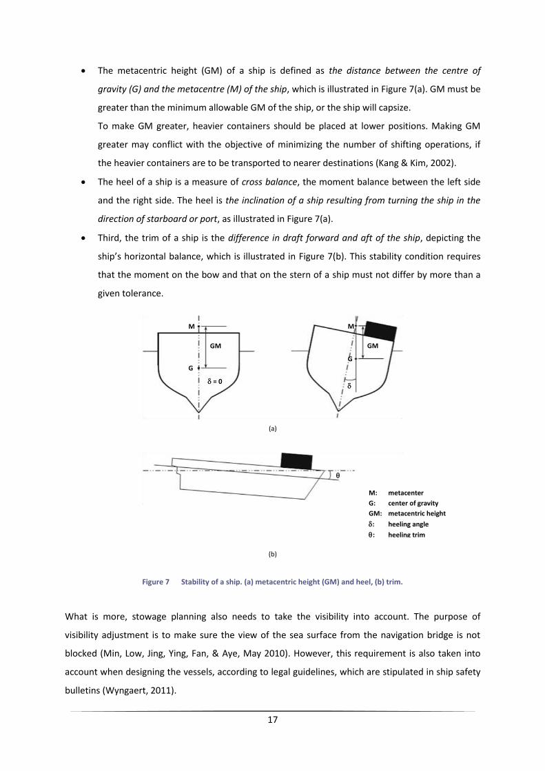
17
The metacentric height (GM) of a ship is defined as the distance between the centre of
gravity (G) and the metacentre (M) of the ship, which is illustrated in Figure 7(a). GM must be
greater than the minimum allowable GM of the ship, or the ship will capsize.
To make GM greater, heavier containers should be placed at lower positions. Making GM
greater may conflict with the objective of minimizing the number of shifting operations, if
the heavier containers are to be transported to nearer destinations (Kang & Kim, 2002).
The heel of a ship is a measure of cross balance, the moment balance between the left side
and the right side. The heel is the inclination of a ship resulting from turning the ship in the
direction of starboard or port, as illustrated in Figure 7(a).
Third, the trim of a ship is the difference in draft forward and aft of the ship, depicting the
ship’s horizontal balance, which is illustrated in Figure 7(b). This stability condition requires
that the moment on the bow and that on the stern of a ship must not differ by more than a
given tolerance.
Figure 7 Stability of a ship. (a) metacentric height (GM) and heel, (b) trim.
What is more, stowage planning also needs to take the visibility into account. The purpose of
visibility adjustment is to make sure the view of the sea surface from the navigation bridge is not
blocked (Min, Low, Jing, Ying, Fan, & Aye, May 2010). However, this requirement is also taken into
account when designing the vessels, according to legal guidelines, which are stipulated in ship safety
bulletins (Wyngaert, 2011).
(b)
M: metacenter
G: center of gravity
GM: metacentric height
: heeling angle
: heeling trim
(a)
M
GM
G
= 0
M
GM
G

18
3.3. Berth and crane allocation
In the introduction, we have already mentioned the necessity of container terminals to
accommodate for the continuous growth of container transportation. However, logistic activities in
container terminals are very expensive and complex by itself because they require the combined use
of several expensive resources (berth, cranes, specialised manpower, straddle carriers, and so on)
(Legato & Mazza, 2001). Therefore, a better management of current resources should be pursued, in
contrast with increasing capacity by terminal expansion or the acquisition of extra handling
equipment. More particularly, quay cranes are the most expensive single unit of handling equipment
in port container terminals. As already stated in the introduction, they cost 5 to 10 million dollars per
quay crane, thus making quay crane availability one of the key operational bottlenecks at ports
(Crainic & Kim, 2007a.). Additionally, berth construction costs are the highest among all relevant cost
factors, making berth space one of the most important resources in container terminals. Therefore,
lots of scientific research focuses on optimising the berth and quay crane allocation problem.
Moreover, the importance of both the berth as well as the crane allocation problem stems from the
fact that the solution of both optimisation problems serves as input for further terminal decision
problems.
An updated literature review of the several models proposed for both the Berth Allocation Problem
and the QCSP can again be found in Stahlbock and Voß (2008). A well-elaborated overview
specifically on BAP and QCSPs, as well as integrated solution approaches can also be found in
Bierwith and Meisel (2010).
3.3.1. Berth Allocation
The task of a berth planning system is to allocate the limited berthing space, organised in a number
of slots among incoming vessels (Meersmans & Dekker, 2001). Constraints usually taken into account
include the ship’s length, the berth’s depth, time windows on the arrival, departure times of vessels,
priority ranking and favourite berthing areas (Vacca, Salani, & Bierlaire, 2010). Moreover, both
Legato and Mazza (2001), as well as Meersmans and Dekker (2001) and Dai et al. (2008) state that
the storage location of outbound/inbound containers to be loaded onto/discharged from the
corresponding vessel is an additional crucial factor to be taken into account when considering the
berth allocation problem. Obviously, it is desirable that vessels berth relatively close to the source
and/or destination point of its containers in the yard. This way, yard transportation costs can be
saved.

19
In literature, several publications concerning the berth allocation problem are available, each
including different assumptions and solution methods. Three broad classifications of the Berth
Allocation Problem can be considered:
In the BAP with continuous berthing space (BAPC), the quay is represented as a continuous
line, allowing berthing for a variable number of vessels, depending on their size. On the other
hand, in the discrete variant of the BAP, each berthing location only allows for one ship at
the time, regardless of its size. The continuous berthing space is for instance described by
Lee et al. (2010), while models for the discrete berth allocation problem (BAPD) recently
were described by Buhrkal et al. (2011).
Additionally, often different assumptions are made concerning vessel inflow. On one hand,
there is the Static Berth Allocation Problem (SBAP) that considers the case where all ships are
already in the port when berths become available. The Dynamic Berth Allocation Problem
(DBAP) on the other hand, allows for ships to arrive during container operations at the port.
Whereas the former can be reduced to an assignment problem, the DBAP can be considered
as a parallel machine scheduling problem where each job has a release time that
corresponds to a ship arrival time. Dai et al. (2008), for instance solve the static berth
allocation problem as a rectangle packing problem while Legato et al. (2001) present a
queuing network and discrete event simulation model for the dynamic arrival-berthing-
departure process of vessels at a container terminal.
Finally, in the static handling time problem the vessel handling time is considered to be
known, whereas in the dynamic (Imai, Chen, Nishimura, & Papadimitriou, 2008) it is a
variable.
Often, the berth allocation problem is modelled simultaneously with the quay crane allocation
problem, either in a hierarchical or integrated way. Further searches on this issue and additional
comments can be found in the next section 3.3.2.
For more information, we recommend the literature review of Golias et al. (2009), as well as
Theofanis et al. (2009) to readers who are interested in this subject, since both papers offer a fairly
complete summary of all recent literature on berth allocation problems.
3.3.2. Crane Allocation
Next to assigning a specific berth space to vessels, operation planners should also decide on assigning
cranes to vessels. As quay cranes are highly expensive (Crainic & Kim, 2007b.), they usually represent
one of the most scarce resources in the terminal. In addition, when adding one more QC, a number

20
of SCs and other handling equipment would be needed accordingly for cooperation, as well as
additional staff (Li & Huo, 2005). Consequently, the quay crane allocation problem aims at efficiently
assigning quay cranes to vessels both in terms of how many QCs to assign, as well as in terms of the
time horizon in which the QCs should be operating on a specific vessel.
Although the berth allocation problem can be elaborated as a stand-alone problem, in literature the
BAP is usually considered in combination with the QCAP. Often, quay cranes are scheduled and then
the berthing position is determined (Park & Kim, 2003; Imai, Chen, Nishimura, & Papadimitriou,
2008). In many other models, the number of assigned QCs is considered to be known beforehand
(Kim & Park, 2004; Moccia, Cordeau, Gaudioso, & Laporte, 2006; Sammarra, Cordeau, Laporte, &
Monaco, 2007; Bierwirth & Meisel, 2009). Besides, this specific example demonstrates the common
trade off that has to be made for many models between the integration of several planning issues
into one and the same model and the level of detail that can be obtained of each element considered
within the model. For instance Raa et al. (2011) present an integrated BAP-QCAP model, while taking
into account many real-life features as well, such as vessel priorities and preferred berthing locations.
Since the objective of many studies is merely to optimise purely mathematical models, this is
unsatisfactory for real-life applications. The MILP model proposed by Raa et al. (2011), on the other
hand, is capable of solving real-life instances in short computation time, making it opportune to
support both operational and tactical decision-making. This is the primary goal of the Tactical Berth
Allocation Problem (TBAP) with Quay Crane Assignment, discussed below.
Introduced by Giallombardo et al. (2008), the TBAP is a model for the integrated optimisation of
berth allocation and quay crane assignment, opposite to the widely used hierarchical model. In the
latter approach, the berth allocation and the quay crane assignment are solved sequentially, thus
based on two separated models for the BAP and the QCAP. The TBAP on the other hand integrates
terminal costs in a more comprehensive way, resulting in a more efficient use of the terminal and its
resources. Due to a longer planning horizon of the TBAP over the BAP, the former can accommodate
shipping lines requests in term of expected berthing times and assigned quay cranes, as well as
penalize for yard-related costs (Giallombardo, Moccia, Salani, & Vacca, 2010). A discussion on both
approaches can be found in Vacca et al. (2010).
3.3.3. Crane Scheduling
Compared to the crane assignment problem, quay crane scheduling is a more operational matter:
planners must assign specific quay cranes to specific tasks (set of containers) and produce a detailed
schedule of the loading and unloading moves for each quay crane (Vacca, Salani, & Bierlaire, 2010).
21
Issues related to interference among cranes, precedence and operational constraints, such as no
overlapping, must also be taken into account.
One important practical constraint within QCSP, often discussed in literature, is the problem of crane
interference, due to the fact that QCs are rail mounted. With respect to crane interference, two
types of constraints can be considered (Bierwirth & Meisel, 2009):
Non-crossing constraint: QCs cannot cross each other.
Safety constraint: Adjacent QCs have to keep a safety margin at any time.
The first constraint can be taken for granted, though shouldn’t be overlooked when formulating a
solution model. In practice, because all QCs are on the same track, only one quay crane can work on
a 40ft bay at any time. Although obvious, this is of great importance in QCSPs as blocking a crane’s
travel route forces idleness, which should be minimized. Zhu et al. (2003, 2006) tackles this problem
more in detail and offer a solution in the form of an Integer Programming model and two algorithms
to solve the CSP.
The second safety constraint requires a certain number of in-between bays between adjacent QCs.
Basically it is perfectly possible to have two QCs working next to each other. However, SCs feeding
the cranes with containers and retrieving unloaded containers should have enough space to get
under the QCs. In practice, a safety margin of one 40ft bay is required (Wyngaert, 2011). In addition,
this safety constraint also applies to idle QCs (Bierwirth & Meisel, 2009) if they are positioned in-
between other QCs for instance.
For a focus on the Quay Crane Scheduling with Non-Interference constraints Problem (QCSNIP) we
refer to Kim and Park (2004), Lee, Wang, & Miao (2008) and Bierwith and Meisel (2009).
3.4. Quay crane efficiency
Quay cranes are the most expensive single unit of handling equipment in port container terminals.
Consequently, any efficiency improvement results in a significantly reduced cost per container
moved. In order to increase the number of containers handled per time unit, among others, a new
generation of container spreaders was invented, as well as the use of double cycling technique was
introduced to avoid empty spreader moves . Both cases are explained below.
Recent efforts to increase crane productivity resulted in cranes with twin or tandem lift ability.
Nowadays, up to four adjacent 20ft containers or two 40ft containers, respectively, can be lifted at
once (Stahlbock & Voß, 2008). The possible lift configurations are displayed in Figure 8 and Figure 9.

22
In order to be able to lift multiple containers simultaneously, cranes are equipped with a specific twin
or tandem container spreader. The most conventional twin spreaders are adjustable and able to lift
single containers up to 45ft long and two adjacent 20ft containers.
Figure 8 Single and twin lift (a) single-lift of 40ft container (b) single-lift of 20ft container (c) twin-lift of two 20 ft containers
Figure 9 Tandem-lift (a) two 40ft containers (b) four 20ft containers
‘Tandem’ means side by side, as opposed to end-to-end ‘twin’ lifts (Figure 8c.). Tandem lift cranes are designed to lift
two containers in tandem (Figure 9a), a single container in tandem with a twin-20’ lift (not depicted here), or four 20’
containers (tandem twin-20 lift, Figure 9b).
Twin lift cranes are designed for faster loading and unloading operations in order to meet the
demand of mega-vessels that requires a larger number of containers to be handled. There are some
operational constraints and areas of concern as well, regarding the use of such a multi-spreader,
which we will state very briefly:
Multiple spreaders cannot be used if stowage is uneven, as the containers have to be leveled
and be in position side-by-side to each other (Goussiatiner, 2007). However, concerning
regular twin-lift spreaders, mechanical systems allow the adjustment to different container
heights (Stahlbock & Voß, 2008).
The use of multi-spreaders impose weight constraints on the lifting capacity of cranes.
Wyngaert (2011) and Goussiatiner (2007) also state that the introduction of multi-spreader
cranes raises safety issues for the gear crew inspecting containers and handling the twist
(a) (b)
(a) (b) (c)

23
locks from all four corners of each container. Gear crew located between tandem-lifted
containers are basically trapped in-between those containers.
Additionally, altering between single and twin lifts requires a slight modification of the spreader
setting. To our knowledge, there is no model taking into account this – rather small, though not
negligible – spreader changeover time.
Another reason for low crane productivity is the temporal decoupling of loading and unloading
operations (single cycling), which requires an unproductive travel of the empty QC spreader in-
between every two consecutive container moves (Meisel & Wichmann, 2010). In contrast, by
alternating loading and unloading operations (double cycling), the number of empty movements of
the QC spreader is reduced and the service of the bay is accelerated. This concept is explained in
Figure 10.
Figure 10 (a) Unloading using single cycling (b) Unloading and loading with double cycling
The use of double-cycling strategies is considered to be a low-cost method to increase capacity. Since
benefits are greater with a larger total number of containers (Goodchild & Daganzo, 2007) and given
the current trend towards larger container vessels, double cycling is a promising technique to
improve quay crane efficiency. Three main operational improvements are considered in literature:
Reduction in crane operating time per vessel. Simulation results point out that for a row of
20 stacks8, on average, there is a 25% reduction in the number of moves over single cycling
(Goodchild & Daganzo, 2007). Consequently, by improving crane productivity, vessels’
turnaround times decrease.
Reduction in the number of landside vehicles and drivers. Double cycling entails that, after a
SC delivers a container to the apron, it can carry an unloaded container from the apron to
8 Large container vessels typically hold up to 20 stacks of containers across the width of the ship.
(a) Single cycling (b) Double cycling
Unload
container
Unload
container Return
without
container
Load
container

24
the container yard, instead of returning without transporting a container. The concept is
explained in Figure 11.
Reduction in the amount of storage equipment required, when using chassis. With double
cycling, we never have both all import as well as all export containers in the container yard
because almost as soon as the unloading of the vessel is started, simultaneously loading of
the vessel is started.
Figure 11 (a) Landside operations when single cycling (b) double cycling
The potential of QC double cycling has been explicitly investigated for the first time in recent studies
of Goodchild (2005) and Goodchild and Daganzo (2006; 2007). The study by Zhang and Kim (2009)
extends this earlier works to a sequencing problem not only for stacks under a hatch cover, but also
for hatches. Although double cycling does not require significant capital investment beyond the
possible additional container handling equipment, it is only used by container terminals to a limited
extent (Goodchild & Daganzo, 2007; Wyngaert, 2011). Hence, further research on the impact of
implementation of double cycling and the integration with other port resources, is required.
3.5. Other operational aspects
In this review we did not tackle every aspect of CT logistics, like the overall container terminal design
itself and the interface with inland transportation, nor the stacking of empty containers. We refer to
Meersmans and Dekker (2001) and Stahlbock and Voß (2008) for an overview of publications
concerning container terminal designs, whereas Crainic et al. (2007a.) recently researched empty
container management.
There are still a number of side issues that were not discussed in this research, just because only a
few papers are available on these topics. For instance, congestion issues in container terminals are
(a) Single cycling (b) Double cycling
Export Import
storage storage
Export Import
storage storage

25
becoming more and more relevant, especially because of the volume increase in container traffic
(Vacca, Salani, & Bierlaire, 2010). In the very recent past, only Han et al. (2008) tackled this issue.
For a comprehensive overview of most of the operational research problems in container terminals,
once again, we refer to the surveys of Meersmans and Dekker (2001), Vis and de Koster (2003) and
Stahlbock and Voß (2008).

26
Chapter 4.
Model design
In the Container Scheduling Problem, a vessel’s arrival and departure configuration of containers in
the vessel’s bay are given. The problem is to find a sequence of container moves that converts the
arrival configuration into the departure configuration within minimum service time of the vessel. In
line with Meisel and Wichmann (2010), the service time in this paper is defined as the total QC
processing time that consists of the time needed for container moves and empty crane movements
in a solution. Additionally, the Quay Crane Scheduling Problem determines the service sequence of
bays of a ship by each QC and the time schedule for the services. Finally, both problems meet during
the actual loading/unloading of a vessel, where the previously assigned QCs handle individual
containers, according to a predetermined sequence.
Since empty movements of the QC spreader can be reduced by alternating loading and unloading
operations (double cycling) and thus reducing the service time of a vessel, double cycling is included
in this model.
4.1. Characteristics
4.1.1. Travelling Salesman Problem
The problem in a TSP is to find the shortest tour that passes through each vertex in a given graph
exactly once, one of the most difficult combinatorial optimisation problems (Moon, Kim, Choi, & Seo,
2002). In addition, when there exists an order in which the vertex should be visited, the problem is
referred to as the travelling salesman problem with precedence constraints, also known as the
sequential ordering problem (SOP) (Montemanni, Smith, & Gambardella, 2008).
The single crane version of the QCSP can be seen as a particular case of the Precedence Constrained
Travelling Salesman Problem (PC-TSP). Indeed, every vertex can be considered as a container, which
has to be handled by the quay crane exactly once. In addition, sequence related constraints are
applied in this QCSP.
This problem has been studied, among others, by Sherali et al. (2006), who propose a formulation for
the asymmetric PC-TSP, based on the enhancement of the basic asymmetric TSP formulation. This
problem has applications in real-world problems as well, such as production planning, single vehicle
routing problems with pick-up and delivery constraints and transportation problems in flexible
manufacturing systems (Sherali, Sarin, & Tsai, 2006).

27
4.1.2. Vehicle Routing Problem and PickUp and Delivery Problems
The Vehicle Routing Problem (VRP) is another combinatorial optimisation problem, seeking to service
a number of customers with a fleet of vehicles. In addition, if a number of goods needs to be moved
from certain pickup locations to other delivery locations, the VRP is extended with Pickup and
Delivery (VRP-PD).
The multiple crane version of the QCSP shares some characteristics with the VRP-PD (Moccia,
Cordeau, Gaudioso, & Laporte, 2006). While loading, the apron can be considered to be the pickup
node, whereas all predefined container slots are delivery nodes, while unloading these similarities
are simply reversed. However, there are some differences, for instance between the time
precedence constraint in the QCSP and the route precedence constraint in the VRP-PD (Moccia,
Cordeau, Gaudioso, & Laporte, 2006). Where a quay crane can start a task, if all preceding tasks are
completed by any quay crane, a vehicle can only visit a delivery node after the pickup node has been
visited by the same vehicle. In addition, the QCSP can rather be seen as a Capacitated VRP, since
quay cranes have limited carrying capacity, namely one single container/delivery at the time9,
whereas vehicles often can visit multiple delivery nodes after one single pickup.
In literature, the static case is often discussed, where all pickup and delivery demands are known on
beforehand. In reality however, the QCSP is often dynamic, because additional demand or changes in
demand might emerge during operations. For a thorough survey on (dynamic) pickup and delivery
problems and more information on both static as well as dynamic modelling, we refer to the recent
research of Berbeglia et al. (2010).
Additionally, in line with Hernández-Pérez and Salazar-González (2009), this paper will assume that
once a container is picked up by a QC it stays locked on the spreader until the container reaches its
destination (either the apron or the predetermined container slot in the vessel). In other words, a
container cannot be dropped at intermediate locations to be later picked up again by the QC. Hence,
this paper will consider the non-preemptive version of the QCSP.
From this point of view, the single crane version of the QCSP can be seen as a particular case of a
Pickup and Delivery problem, namely the Stacker Crane Problem (SCP). The SCP is a pickup and
delivery problem which involves only one vehicle. It can deal with only one demand unit at the same
time and was recently described by Quillot et al. (2010).
9 More particular, one container move per time, since twin or tandem lifts only count as one movement as well.

28
4.1.3. Parallel Machine Scheduling Problem with Sequence-Dependent Setup Times
In the Parallel Machine Scheduling Problem (PMSP), one of the most difficult classes among
scheduling problems, a set of independent jobs have to be processed by exactly one of parallel
machines. Each machine can process no more than one job at a time. Different optimisation criteria
can be considered; for instance the minimization of maximum lateness and the minimization of the
sum of completion times, recently discussed by Gacias et al. (2010).
As for the multiple machine characteristics, roughly three categories can be considered, according to
the processing time of a job (Chaudhry, 2010):
Identical parallel machines: processing times of a job are the same on all the machines.
Uniform parallel machines: the speeds of the machines are different, that is, the processing
times of jobs on a machine are proportional to a ratio given for the machine.
Unrelated parallel machines: processing times of a job on different machines are arbitrarily
different.
Other job characteristics can also be considered within the PMSP: pre-emption, precedence
constraints, due date, ready time, ... If precedence relations between the jobs and setup times are
considered when different jobs are sequenced on the same machine, then these constraints must be
satisfied as well. Additionally, if pre-emption is not allowed, each job is continually processed during
its complete processing time, on the same machine. In PMSPs, these processing times are often
known as priori.
From this point of view, the QCSP can be formally defined as a an Identical Parallel Machine
Scheduling Problem with precedence constraints and with sequence-dependent setup times. Indeed, a
set of different containers have to be handled by exactly one of parallel identical QCs. In
addition, since containers in a stack can only be reached from the top, and a vessel’s deck and hold
are separated by hatch covers, precedence constraints do apply. Furthermore, prior to processing
each job, a sequence-dependent setup time (SDST) , independent of the machine, is incurred
when container is handled immediately after container by the same quay crane (Ying & Cheng,
2010). However, since efficiency rates of QCs are largely determined by the experience and skills of
the crane operators, the problem can also be categorized within the uniform MPSPs (Sammarra,
Cordeau, Laporte, & Monaco, 2007).
Additionally, the berth allocation problem is one of the parallel machine scheduling problems as well.
In this case, a job and a machine can be treated as a ship and a berth, respectively (Imai, Nishimura,
& Papadimitriou, 2001).
29
4.1.4. NP-hardness
This section briefly discusses the computational complexity of the QCSP, to justify the use of heuristic
algorithms when solving the problem. The models proposed below will share some characteristics of
the commonly known TSP, belonging to the class of NP-hard10 problems (Moon, Kim, Choi, & Seo,
2002) and the VRP. Moreover, there will be especially strong similarities with the PMSP, which is
known to be NP-hard as well (Sammarra, Cordeau, Laporte, & Monaco, 2007; Ying & Cheng, 2010;
Gacias, Artigues, & Lopez, 2010). If a problem is proved to be NP-hard, heuristic algorithms are
needed to obtain near-optimal solutions for the problem.
It is not the intention of this paper to dig deeper into the concept of NP-hardness, nor to prove the
NP-hardness of the QCSP. However, Bierwith and Meisel (2009) do give notice of the NP-hardness of
the QCSP, whereas Lee et al. (2010) even give proof of NP-completeness of their QCSP model.
Because of this, and since our QCSP model greatly resembles other NP-hard problems, we presume
the proposed QCSP model is proved to be NP-complete, or at least near-NP-hard. As a result, the use
of heuristic solution methods, to find near optimal solutions is justified.
4.2. Assumptions
Some assumptions are made in the model. They have a dual purpose. On the one hand, these
assumptions are being made in order to clearly mark out the problem definition, while on the other
hand this makes it possible to put up a number of simplifications. The assumptions made are
explained in the following:
- Both the vessel’s stowage plan on arrival, as well as on departure are assumed to be known in
advance. Consequently, the problem is situated merely in determining the sequence in which
containers will be handled. In addition, we assume that weight and balance constraints are
already taken into account during stowage planning.
- Multiple QCs are assumed to work simultaneously – while of course taking the non-interference
constraint into account – at the same efficiency rate. In other words, we assume that all crane
operators are uniformly skilled, which results in equal container handling times on all QCs. Notice
that in reality, this is often not the case (Wyngaert, 2011), which entails an additional difficulty in
the QCSP.
10
Non-deterministic polynomial-time hard. NP is one of the most fundamental complexity classes in 10
computational complexity theory.

30
- The QC spreader is supposed to manage all standard container sizes. In addition, all containers are
assumed to be of an equal height, as the containers have to be levelled to allow for twin lifts11.
- The model does not take yard operations into account. As a result, it is assumed that there is no
waiting time to load or unload containers. SCs or other handling equipment thus deliver the right
containers on time and immediately take away discharged containers from under the QCs, which
in reality is often not the case. Consequently, the QC service time depends on the move sequence
of the QC and is not influenced by yard transport operations.
- Similar to Meisel and Wichmann (2010), internal reshuffles are omitted from the model, for
reasons of practicability. The benefit of such moves indeed is limited, because the temporarily
stored containers hinder the processing of the occupied stacks and container positions must be
tracked all the time. Accordingly, the model only assumes external reshuffles: reshuffle containers
in a stack are unloaded from the vessel to the quay and reloaded at a later point in time.
- Two 20ft containers side-by-side to each other in the same 40ft bay are assumed to be taken in
twin lift. In the model, this counts as one single QC move, since a twin lift is similar to handling
one 40ft container. By this assumption, the model actually requires the number of twin-lifts to be
maximized, eventually increasing crane productivity (Yeh, Yeh, & Choudhury, 2007).
- The model does not penalize for spreader travel time along the width of the vessel. In other
words, the actual handling time of two identical containers, for instance positioned in rows 10 and
09 respectively, is assumed to be equal.
- The model allows for deck hatches, large steel plates that separate above-deck and below-deck
storage. They normally cover one-third of a single 40ft bay (Goodchild & Daganzo, 2006; Zhang &
Kim, 2009; Wyngaert, 2011). However, the model assumes deck hatches to cover an entire bay,
for the purpose of simplification. Meisel and Wichmann (2010) for instance did not include
hatches in their model, whereas Zhang and Kim (2009) did.
Moreover, in practice it is not customary to take off only part of the hatch cover, although this
would be possible in theory. Partially removed hatches indeed are not practical to the crane
operator, as this would lead to reduced visibility of the containers below deck.
- In practice it might be possible that a vessel has to be replaced after mooring, because of the
depth of the water and/or because another vessel demands the berth location. However, we will
assume that, once a vessel is moored at the quay, it will stay in that position until the end of its
11
Otherwise, the QC spreader is assumed to be capable of adjusting to different container heights.

31
service. Indeed, we also assume that the vessel’s berth location is already known – and
optimised – in advance.
4.3. A first model
4.3.1. Modelling approach
This first model of the QC scheduling problem is based on the Kim and Park (2004) mixed integer
model, which is solved exactly by a branch-and-bound scheme on a reduced solution space. Their
model is structured in such a way that a task is defined as a group of homogeneous containers to be
handled. Afterwards, Moccia et al. (2006) developed an improved formulation of the QCSP, capable
of solving small and medium size instances through a branch-and-cut algorithm.
The Kim and Park (2004) model works very well on instances with two cranes and up to ten to fifteen
tasks, whereas it fails on instances with three cranes and twenty to twenty-five tasks. On the other
hand, the branch-and-cut algorithm of Moccia et al. (2006) has a higher overall efficiency, both in
terms of solution quality and of computation time. In order to overcome the fast growth of the
solution time with the size of the instances, Sammarra et al. (2007) propose tackling the QCSP as a
vehicle routing problem, using a tabu search-based heuristic to solve the problem. Their solution
method provides a good compromise between solution quality and computation time.
Although this formulation of the QCSP is based on the model developed by Kim and Park (2004),
taking into account some modifications made by Moccia et al. (2006), there are dissimilarities. This
model differs to the extent that a direct time dependence was incorporated with regard to certain
variables. Additionally, spreader setup times and the impact of double cycling are also taken into
account, through sequence dependent setup times and double cycling penalties, respectively.
4.3.2. Mathematical formulation
The following notations are used for mathematical formulation.
Indices:
Containers to be handled
The handling of containers and will be considered to be the initial and final task of
each QC, respectively.
QCs, where . QCs are ordered in an increasing order of their relative locations
in the direction of increasing ship-bay numbers12
Certain moment or within the total makespan
12
40ft ship-bay numbers
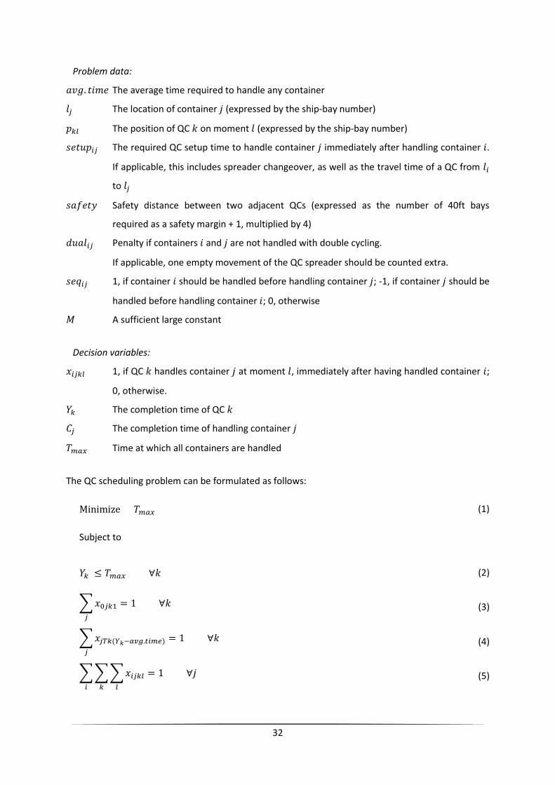
32
Problem data:
The average time required to handle any container
The location of container (expressed by the ship-bay number)
The position of QC on moment (expressed by the ship-bay number)
The required QC setup time to handle container immediately after handling container .
If applicable, this includes spreader changeover, as well as the travel time of a QC from
to
Safety distance between two adjacent QCs (expressed as the number of 40ft bays
required as a safety margin + 1, multiplied by 4)
Penalty if containers and are not handled with double cycling.
If applicable, one empty movement of the QC spreader should be counted extra.
1, if container should be handled before handling container ; -1, if container should be
handled before handling container ; 0, otherwise
A sufficient large constant
Decision variables:
1, if QC handles container at moment , immediately after having handled container ;
0, otherwise.
The completion time of QC
The completion time of handling container
Time at which all containers are handled
The QC scheduling problem can be formulated as follows:
(1)
Subject to
(2)
(3)
(4)
(5)
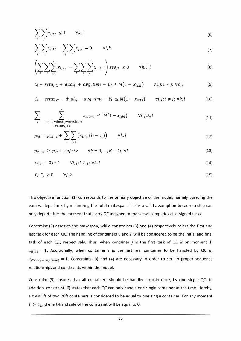
33
(6)
(7)
(8)
(9)
(10)
(11)
(12)
(13)
(14)
(15)
This objective function (1) corresponds to the primary objective of the model, namely pursuing the
earliest departure, by minimizing the total makespan. This is a valid assumption because a ship can
only depart after the moment that every QC assigned to the vessel completes all assigned tasks.
Constraint (2) assesses the makespan, while constraints (3) and (4) respectively select the first and
last task for each QC. The handling of containers and will be considered to be the initial and final
task of each QC, respectively. Thus, when container is the first task of QC on moment ,
. Additionally, when container is the last real container to be handled by QC ,
. Constraints (3) and (4) are necessary in order to set up proper sequence
relationships and constraints within the model.
Constraint (5) ensures that all containers should be handled exactly once, by one single QC. In
addition, constraint (6) states that each QC can only handle one single container at the time. Hereby,
a twin lift of two 20ft containers is considered to be equal to one single container. For any moment
, the left-hand side of the constraint will be equal to 0.

34
In line with Kim and Park (2004), a flow balance constraint is defined by constraint (7), guaranteeing
that tasks are performed in well-defined sequences. Basically, it states that every task on any QC
should be preceded and followed by another task. Therefore, constraints (3) and (4) are necessary as
start condition as well as final condition of each QC. In addition, constraint (8) eliminates sequences
contrary to the predetermined sequences. The latter constraint is of key importance, since it allows
to incorporate hatch covers to the model and other precedence relationships among containers. For
instance all containers on deck must be unloaded before tasks in the hold of the same ship-bay can
be performed. This example is elaborated below.
If a container is located on-deck and container is located in the hold of the same bay, then will be
set to during preprocessing (container should be handled before container ). If the precedence
relations are respected, the left-hand side of constraint (8) consequently will equal 1 (case IV). However, if
in such a case container is handled before container , the left-hand side of the constraint will equal
at a certain moment l, which cannot be allowed because of constraint (8)(case VII). In the opposite case,
will be set to during preprocessing, leading to the same results (cases IX and VI, respectively).
In cases where there is no precedence relationship between two containers and (eg. two containers in
the same bay, above deck, in a different row), the left-hand side of constraint (8) will always equal 0 (cases
II, V, VIII and XI). Likewise, when containers and either both have been handled, as well as both not have
been handled before moment , the left-hand side will equal 0, regardless their precedence relationship
(cases I, III, X and XII). All possible combinations are listed in Table 3 below.
I 1 1 1 0
II 1 1 0 0
III 1 1 -1 0
IV 1 0 1 1
V 1 0 0 0
VI 1 0 -1 -1
VII 0 1 1 -1
VIII 0 1 0 0
IX 0 1 -1 1
X 0 0 1 0
XI 0 0 0 0
XII 0 0 -1 0
Table 3 Possible combinations of variables for constraint (8) on a certain moment m
Constraint (9) determines the completion time for each task , whereas in combination with
constraint (8), it also denotes that task should be completed before task , if necessary. Likewise,
completion times for each QC are determined by constraint (10).

35
Similarly, constraint (11) determines the exact moment at which decision the variable can be set
equal to one. To be more precise, this restriction takes into account the handling time of the
previous container, as well as related setup times and double cycling penalties.
By constraints (12) and (13), interference among QCs can be avoided. The former determines the
location of QC at any moment , whereas constraint (13) positions two adjacent QCs apart from
each other by a predefined interspace. Note that QCs are ordered in an increasing order of their
relative locations, in the direction of increasing ship-bay number, ensuring the correctness of
constraint (13). On the other hand, by comparing the positions of adjacent QCs two-by-two, this also
ensures the non-crossing constraint (Bierwirth & Meisel, 2009).
The formulation of constraints (1)-(15) is a Mixed-Integer Linear Program, which is expected to
require quite some computation time for practical use.
4.3.3. The interference constraint
After verifying the Kim and Park (2004) mixed integer model, the proposed inequalities to counter
interference were found not to be completely accurate (Moccia, Cordeau, Gaudioso, & Laporte,
2006). The Kim and Park (2004) model only avoids collisions between QCs working on tasks belonging
to the same bay by forcing non-simultaneity of two tasks and in the same bay. However, they do
not take the movement time of QCs into account, making the model unable to detect collisions.
Below we will prove the validity of constraints (12) and (13), using a simple example, depictured in
Figure 12. In this example, two QCs are each working on a vessel, in bay 02 and bay 10, respectively.
Figure 12 Interference constraint example
Assume two containers 1 and 2 with location data = 02 and = 06, respectively. Note that, as
stated above, these locations refer to ship-bay numbers. Furthermore, we assume QC1 busy working
on bay 02, while assuming QC2 fixed working on containers in bay 10, as presented in the figure
above. Additionally, the safety margin in-between two adjacent QCs is set to one 40ft bay, resulting
in a parameter equal to 8. Note that the reason to do so is because 40ft ship-bay numbers
Bay
22 18 14 10 06 02
Bay
22 18 14 10 06 02
Quay Crane n°
2 1
Quay Crane n°
2 1

36
increase by leaps of 4. In this initial situation, the following (in)equalities are applicable when QC1
would be working on container 1:
l k
l=1 1 -
2
Table 4 Initial situation for the interference constraint example
In the case that container 2 would be assigned to QC1 at the next moment – while neglecting
handling times and/or setup times, – would equal 1 in the model, leading to the values below:
l k
l=2 1 -
2
Table 5 Interference situation for the interference constraint example
This situation would clearly lead to interference, which will be noticed through restriction (13).
Consequently, should be set equal to , until there is enough space in-between both QCs to
displace QC1. With , the model again would be feasible, as would be set to bay 02 and
as a result, again would equal + 8 allowed by restriction (13). Indeed,
02 + 0 (06-02) , so that 10 is equal to 02 + 8 = 10.
4.4. A second model
4.4.1. Modelling approach
Next to the first model we developed a second model, presented in this section. While this model
may look very complicated at first sight, its main objective is to be much more comprehensible than
the first model, described in the previous section 4.3. Moreover, what follows in this section is
nothing more than the mathematical representation of a very intuitive and pragmatic model.
While perfectly in line with reality, the model is both easy to visualize as well as to incorporate most
notable practical constraints within the QCSP. Double cycles, as well as sequence-dependent setup
times or interference constraints that are included in this model, are visually represented.
Furthermore, the model differentiates between unloading and loading actions, increasing the
practicality of the model. While an unloading action is represented by an -variable, a loading action

37
is expressed through a -variable. In addition, in this model the time horizon, and thus every working
shift, is discretized in time steps. Because of this, it is possible to verify the correctness of each
constraint, at every time unit.
In this model, one time unit corresponds to approximately 30 seconds in reality. However, the exact
duration of one time unit is not of great importance, though the ratios among various QC actions are.
Therefore, we rely on numbers from literature and our own measurements in the Port of Zeebrugge.
In literature, it is stated that the average QC cycle time for single cycling amounts 1 minute and 45
seconds, whereas the average double cycle took 2 minutes and 50 seconds (Efficient Marine
Terminal Trial at the Port of Tacoma in 2003) (Goodchild & Daganzo, 2007). In addition, thanks to the
telescopic motion of container spreaders, spreader changeovers from 20ft to 40ft containers take
approximately 28 seconds (Bromma, 2011). Finally, the travel time of a quay crane between two 40ft
bays is about 1 minute according to Lee et al. (2008), whereas our measurements averaged about 2
minutes and 35 seconds. The large difference between the last two numbers can be explained by a
different measuring method. Whereas the actual travel time of a QC might truly amount 1 minute, it
takes quite some more time before the crane operator can actually handle the next container (due to
fine-tuning of its position, stability in the wind, ...). Additionally, since the model aims at minimizing
the number of displacements per QC, a larger time penalty of 9 time units was chosen as travel time
of a quay crane. Moreover, the number of time units depends of course on how far the QC should
move. More specifically, a fixed large penalty was chosen, to minimize the number of QC
displacements, as well as a variable penalty, linked to the number of 40ft bays the QC has to move.
This variable penalty is set to 1 time unit for each 40ft bay distance moved.
As the duration of a spreader telescopic changeover (28 seconds) is the smallest, this will be the
standard for one single time unit. Therefore, with an approximated single time unit of 30 seconds,
the following time dimensions are obtained:
Action Average Approximation Time Units
Spreader setup 28 sec 30 sec 1 (per action)
Single Cycle 1 min 45 sec 1 min 30 sec 3 (per action)
Empty movement - 30 sec 1 (per action)
Double Cycle 2 min 50 sec 3 min 6 (per action)
QC displacement - (Fixed part) 4 min 30 sec 9 (per action)
1 min 00 sec (Variable part) 30 sec 1 (per 40ft bay)
Table 6 Time units per QC action

38
When two loading or unloading actions are scheduled consecutively (single cycling), one empty
movement should be counted extra. Practically, one time unit of idle time will be inserted between
both actions. An example in section 4.4.2 will clarify this concept. However, this unit of idle time is
not inserted when double cycling (when directly after loading, an unload action is performed, and
vice versa). As a result, when executing a dual loop, the efficiency gain is one time unit. More
information on the representation of the second model is given in the section below.
4.4.2. Solution representation
The model and solution representation is explained using a simple example, described below. It
concerns an easy loading/unloading problem in two bays, namely bay 06 and 26. We will consider
two quay cranes, each working on one of the bays. In bay 06, two 40ft containers should be
unloaded, after which two other 40ft containers should be loaded. In addition, one of the containers
is located above deck, while the other is located in the hold. As for bay 26, the containers to be
unloaded and loaded on deck are 40ft containers, whereas containers to be unloaded and loaded in
the hold are two 20ft containers. However, we consider these as one container, since they can be
handled in twin lift, with one QC movement. The problem is depictured in Figure 13.
Figure 13 An easy QCSP example
Because hatch covers are used in this example, we can draw some precedence constraints as follows:
In bay 06: Unloading[3] Unloading [4] Loading [8] Loading [7]
In bay 26: Unloading[1] Unloading [2] Loading [6] Loading [5]
Regarding the interference constraint, this will not cause a problem in our example, since there are four
bays in between bay 06 and 26, while a safety margin of only one 40ft bay is actually required. In addition,
since all containers to be handled in bay 06 are 40ft containers, no setup times are needed. In bay 26 on the
other hand, the following setups should be considered:
Bay 26 Bay 06
Arrival
configuration
Departure
configuration
1 5
2 2 6 6
3 7
4 8
Arrival
configuration
Departure
configuration

39
In bay 26: [1] [2] [6] [5]
(40ft) [SETUP] (20ft-20ft) [X] (20ft-20ft) [SETUP] (40ft)
What is more, double cycling is only possible in both bays between the last unloading action and the first
loading action. As a result, one empty movement should be counted between the single loops.
Consequently, one time unit of idle time should be inserted between two similar actions. The solution to
this problem (with two quay cranes) is visualized in Figure 14.
Figure 14 Solution representation of the easy QCSP example (Information duplication per QC)
As can be seen above, this small QCSP will be finished after 16 time periods, or within 8 minutes in
particular. Moreover, from the figure we can deduce that QC2 finishes two time units earlier than QC1,
since the latter had to include two time units of setup time.
What is more, some of the practical constraints can be deduced from Figure 14 on sight.
Each QC can only have one action status at the time. A QC can either be handling containers ( or -
variables), performing a setup, be idle, or non-active.
In the representation, this means that the sum of each horizontal line (including the ‘ ’-
variable) should equal exactly one, for each QC.
x y x y x y x y x y x y x y x y x y x y x y x y x y x y x y x y
1 1 1
2 1 1
3 1 1
4 1 1
5 1 1
6 1 1
7 1 1
8 1 1
9 1 1
10 1 1
11 1 1
12 1 1
13 1 1
14 1 1
15 1 1
16 1 1
17 1
18
19
QC 1
26
3 4 8
Idle
setu
p
1 2 6 85
Bay N°
06
5 67
do
ne
Container N°
3
QC 2
Idle
setu
p
Bay N°
06 26
Container N°
1 2 4 7

40
Each container should be handled exactly once
In the representation, this means that the sum of a vertical line (for each container) should equal
exactly three for one of the quay cranes. Vertical summations can equal zero for a crane, but the
total sum per container over all QCs should be three.
For information, the solution to this problem with one single quay crane is visualized in Appendix 10.5. In
this case, the QCSP will be finished after 44 time periods (22 minutes). Of course, this is more than the sum
of the individual QC completion times presented above (16 + 14 time units), since the crane will have to
move in-between both bays. As a result, 14 additional time units are counted extra, namely 9 TUs for the
QC displacement and 5 extra TUs, since the QC has to move along 5 bays.
In addition, we can also check on sight whether an empty movement (under the form of ) has been
inserted between two identical QC moves ( - or - ). Furthermore, in this setting it is quite hard to check
crane interference instantly. However, by slightly changing the representation of the solution, crane
interference can be verified more easily. In order to do so, action information can easily be duplicated per
bay, instead of per QC (as seen above in Figure 14). The second way of representing the QCSP, specifically
designed for visual inspection of the interference constraint, is shown below in Figure 15.
Figure 15 Solution representation of the easy QCSP example (Information duplication per bay)
In the example presented above, crane interference of course won’t be a problem. However, interference
occurs when the containers to be handled would be located in bay 06 and bay 10 instead of bay 06 and 26,
respectively. In general, an additional practical constraints can be deduced on sight, applicable to the
second way of visualization (Figure 15):
x y x y x y x y x y x y x y x y x y x y x y x y x y x y x y x y
1 1 1
2 1 1
3 1 1
4 1 1
5 1 1
6 1 1⋮
⋮
14 1 1
15 1 1
16 1 1
17 1
18
idle
setu
p
idle
setu
p
idle
setu
p
QC N°QC N°
1 2 1 2
3 4 7 85 6 3 4 7 81 2 5 6 1 2idle
setu
pContainer N° Container N° Container N° Container N°do
ne
Bay 06 Bay 26

41
Non-interference constraint: Adjacent QCs have to keep a safety margin of one 40ft bay at any time.
In the representation, this means that the sum of each horizontal line (including the ‘ ’-
variable) should equal exactly one, for every two adjacent bays.
Of course, other representation methods are possible as well. It would, for instance, even be possible to
duplicate information per container or make other combinations of bay-crane-container. However, we do
realize that for large instances these representations might not always be very obvious, nor helpful.
This brings us again to one of the above-mentioned statements. The main objective of this model is
to be very intuitive and understandable, unlike the first model presented in section 4.3. As a result,
this model is quite detailed, and consequently has many variables. Therefore, this modelling
approach is only applicable to small problems. Large problem instances result in complex
representations, whilst being very hard to solve using this model. Furthermore, the mathematical
formulation of the model, presented below, looks rather illogical and complicated as well.
4.4.3. Mathematical formulation
The following notations are used for mathematical formulation.
Indices:
Containers to be handled
QCs, where . QCs are ordered in an increasing order of their relative locations
in the direction of increasing ship-bay numbers
Certain moment or within the total makespan
Problem data:
The average time required to handle any container
The location of container (expressed by the ship-bay number)
The position of QC on moment (expressed by the ship-bay number)
The required QC setup time to handle container immediately after handling container .
If applicable, this includes spreader changeover, as well as the travel time of a QC from
to .
1, if container should be unloaded; 0, otherwise
1, if container should be loaded; 0, otherwise
1, if container should be handled before handling container ; -1, if container should be
handled before handling container ; 0, otherwise
Safety distance between two adjacent QCs (expressed as the number of 40ft bays
required as a safety margin + 1, multiplied by 4)

42
A sufficient large constant
Total number of containers to be handled
Number of time units that exceeds the maximum completion time (= end of the
timeframe)
Decision variables:
1, if QC unloads container at moment ; 0, otherwise.
1, if QC loads container at moment ; 0, otherwise.
1, if crane is doing a setup at moment ; 0 otherwise
1, if crane is idle at moment ; 0, otherwise
1, if all containers are handled at a certain moment ; 0 otherwise
The completion time of QC
Time at which all containers are handled
The QC scheduling problem can be formulated as follows:
(16)
Subject to
(17)
(18)
(19)
(20)
(21)
(22)
(23)
(24)

43
(25)
(26)
(27)
(28)
(29)
(30)
(31)
(32)
(33)
(34)
(35)
(36)
(37)
(38)
(39)

44
This objective function (16) again aims to minimize the total makespan, in order to obtain the earliest
departure possible.
Constraints (17) and (18) make sure that all containers should be handled exactly once, by one single
QC. In addition, these constraints ensure that the type of handling is respected. Import containers
should be unloaded, whereas export containers should be loaded. To achieve this, decision variables
and
for a certain container can only be equal to if and
respectively. In addition, nonpreemption is guaranteed through constraints (19) and (20). Every
action, unloading and loading respectively, should be finished at once after starting, without
intermission.
Constraint (21) determines one of the four possible QC action statuses while at once stating that a
crane can handle only one single container at the time. A QC can be handling a container - either
unloading or loading ( or
respectively), - changing its spreader settings or moving
along the quay ( ), or can be idle (
). A quay crane is idle when performing empty QC
spreader movements or when the QC has no more containers to handle while other QCs are still
busy. Finally, a QC can also be non-active, which will only occur for all QCs simultaneously, if all
containers are handled ( ).
Single and double cycling rules are incorporated through restriction (22) till (26). If altering between
loading and unloading is not possible, through the combination of restrictions (21) till (26), one
empty movement of the QC spreader should be counted extra, through the decision variable .
In short there are three possible infeasibilities, restricted by the inequalities mentioned above. First,
restrictions (22) and (23) make it impossible that a load and unload action are followed by a load and
unload action, respectively, without intermission of idleness. Second, restrictions (24) and (25) state
that, in cases of single cycling, it is impossible to avoid idleness, through the use of the decision
variable instead of
. Finally, inequality (26) defines the right sequence of idleness and setup
time within the model. A setup ( ) will always be done in between two container handlings, and if
applicable, after a period of idleness. These rules will be further explained in section 4.4.4.
Restrictions (27) till (29) deal with precedence constraints. If there exists a sequence
between two containers and , then, at a certain moment , three different scenarios are possible.
First, either both containers are not yet unloaded or, second, both containers were already unloaded
before that particular moment . In the third case, the first container should be unloaded before a
certain moment , after which the second container can be assigned to a specific crane. A fourth
scenario, in which (resp. ) and where container (resp. ) is already handled and

45
container (resp. ) is not, is infeasible, and thus excluded by constraints (27) till (29). In addition,
these constraints also determine that two containers and can never be handled simultaneously -
by the same QC or different QCs, - if there exists a sequence between those containers. If
no special sequence constraints are imposed, the left hand side of these constraints will equal zero.
The duration of the setup times is determined by constraints (30) till (33). Between two containers
and , the sum of all setup periods should be greater than or equal to the predefined setup times
. However, since the objective is to minimize the total makespan, the total number of setup
periods will be minimized, thus set equal to the actual predefined setup time.
Interference among QCs is avoided through constraints (34) and (35). The former determines the
location of QC at any moment , whereas constraint (35) positions two adjacent QCs apart from
each other by a predefined interspace. The non-crossing constraint is ensured as well, by comparing
the positions of adjacent QCs two-by-two.
Finally, constraints (36) and (37) set the termination binary equal to and , respectively,
when necessary.
The formulation of constraints (16)-(39) again is a Mixed-Integer Linear Program. Since a lot of
different decision variables are used, this problem is expected to require excessive computation time
for practical use. At any moment, two decision variables are to be set, for each QC (namely and
). In addition, because loading and unloading operations are treated separately, for each QC,
and for each container (!), two additional decision variables (namely and
) should be
determined as well. In conclusion, we can say that this model indeed is intuitive and very
understandable, but only applicable to small problem instances. It is suitable to clarify the quay crane
scheduling problem using a small example, though not usable for real-life problems.
4.4.4. Constraint examples
Given the mathematical complexity of the model presented above, this section links the
mathematical constraints to the visual representation. Using small examples, two of the constraints
will be explained below.
Non-preemption Constraints (19) and (20)
Every action, unloading and loading respectively, should be finished at once after starting, without
intermission. Or, in terms of visualization, within a vertical column, decision variables or
should always form blocks of three consecutive variables equal to one. In other words, a

46
series of variables or
equal to one should never be interrupted. A practical example,
demonstrating the correctness of constraint (19), is visualized in Figure 16 below. Note that this
constraint should be valid for every container and crane on every moment in time. In the
example, we assume two different containers handled by two different QCs, while all other
constraints are satisfied.
Figure 16 Examples on the non-preemption constraint
As can be seen in Figure 16, container 1 is handled correctly according to the model, whereas
container 2 is not. Such arrangements will yield the following results, according to constraint (19):
Container 1
1 0 0 0 1 0
2 1 1 0,33 1 0,66
3 1 2 0,66 1 0,33
4 1 3 1 0 0
5 0 3 1 0 -1
6 0 3 1 0 -1
Container 2
1 0 0 0 1 0
2 1 1 0,33 1 0,66
3 1 2 0,66 0 0,33
4 0 2 0,66 1 -0,66
5 1 3 1 0 0
6 0 3 1 0 -1
Table 7 Results of the examples on the non-preemption constraint
As can be seen in the table above, the left-hand side of constraint (19) is always greater than the
right-hand side for container 1, as it should be. In a case of preemption, present in the way of
m x y x y m x y x y m x y x y m x y x y m x y x y m x y x y
1 1 1 1 1 1⋮ ⋮ ⋮ ⋮ ⋮ ⋮
l
⋮ ⋮ ⋮ ⋮ ⋮
l+1 1 1 l 1 1
⋮
1 1
⋮
1 1
⋮
1 1
⋮
1 1
1 1 l+1 1 1 l 1 1
⋮
1 1
⋮
1 1
⋮
1 1
1 1 l+1 1 l 1
⋮
1
⋮
1
1 1 1 l+1 1 l 1
⋮
1
l+1 l
l+1
Moment 5 Moment 6
1 2
Moment 1 Moment 2 Moment 3 Moment 4
1 2 1 21 2211 2

47
handling container 2, there will always be at least one moment where constraint (19) is not
satisfied – moment 3 in the example above.
Single and double cycling rules Constraints (22) until (26)
When single cycling, one empty movement of the QC spreader should be counted extra in-
between two movements. In short three possible errors can be made, illustrated below by Figure
17. A first error is for example a situation in which no idleness is inserted between two
consecutive load or unload actions. This situation is restricted by inequalities (22) and (23).
Second, it would be wrong to insert only setup time (through the decision variable ), without an
idle time unit preceding this setup time. This is prohibited by restrictions (24) and (25). Finally,
inequality (26) defines the right sequence of idleness and setup time within the model. A setup
( ), if necessary, is always inserted in between two container handlings, and if applicable, after a
period of idleness.
Figure 17 Examples on single and double cycling rules
x y x y x y x y x y x y x y x y x y x y
l1
l2
l3 1 1 l3 1 1 1
l4 1 1 l4 1 1 1
l5 1 1 l5 1 1 1
l6 1 1 1 l6 1 l6 1
l7 1 1 1 1 1
l8 1 1 1 1 1
l9 1 1 1 1
l10 1 1
l11
x y x y x y x y
l1
l2
l3 1 1
l4 1 1
l5 1 1
l6 1 1
l7 1 1
l8 1 1
l9 1
l10
l11
Correct 4
setu
p 1 2
Double Cycling
Correct 3
idle
setu
p 1 2
idle
idle
setu
p
idle
idle
setu
p
idle
setu
p
idle
setu
p
setu
p 1 2
Error 3
1 2 1 2 1 2 1 2
Correct 1 Correct 2 Error 1 Error 2
Single Cycling

48
The first error is detected by constraint (23) at moment l3, as well as moment l4 and l5. At these
points in time, the left-hand side of the constraint (
) equals four, since all
containers should be taken into account, per QC. At moment l6, an error type 2 is detected by
constraint (25). As a result,
equals 3, which is greater than 2. At the same
moment, the left-hand side of constraint (26), namely
, equals 2. As a result, the
third error is detected as well. The full table with results can be found below, proving that these
constraints are also applicable to double cycling.
.
Co
rrec
t 1
Co
rrec
t 2
Erro
r 1
Erro
r 2
Erro
r 3
Co
rrec
t 3
Co
rrec
t 4
Co
rrec
t 1
Co
rrec
t 2
Erro
r 1
Erro
r 2
Erro
r 3
Co
rrec
t 3
Co
rrec
t 4
Co
rrec
t 1
Co
rrec
t 2
Erro
r 1
Erro
r 2
Erro
r 3
Co
rrec
t 3
Co
rrec
t 4
l1 2 2 2 2 2 0 0 0 0 0 0 0 0 0 0 0 0 0 0 0 0
l2 3 3 3 3 3 0 0 0 0 0 0 0 0 0 0 0 0 0 0 0 0
l3 3 3 4 3 3 1 0 0 0 0 0 0 0 0 0 0 0 0 0 0 0
l4 3 2 4 3 2 2 1 1 1 1 1 1 0 0 0 0 0 0 0 0 0
l5 3 2 4 3 2 3 2 1 1 2 1 1 1 0 1 1 0 0 0 0 0
l6 3 2 3 3 2 3 3 2 1 2 3 2 1 2 0 0 0 1 2 0 1
l7 3 3 2 3 3 2 3 1 2 1 1 1 1 1 0 1 0 0 0 0 0
l8 2 3 1 2 3 1 2 1 1 0 1 1 0 1 0 0 0 0 0 0 0
l9 1 2 0 1 2 0 1 0 1 0 0 1 0 0 0 0 0 0 0 0 0
l10 0 1 0 0 1 0 0 0 0 0 0 0 0 0 0 0 0 0 0 0 0
l11 0 0 0 0 0 0 0 0 0 0 0 0 0 0 0 0 0 0 0 0 0
Table 8 Results of the examples on the single cycling and double cycling rules
4.5. Small comparison between both models
Although both models represent a Mixed-Integer Linear Program, quite some differences are
notable. Whereas the first model (MDL1) is rather basic, showing only little detail, the second model
(MDL2) goes further into detail. MDL2 not only treats loading and unloading operations separately,
but deals with discrete single time units as well. Furthermore, all special practical constraints (double
cycling, sequence dependent setup times, sequence constraints, setup times, …) are included in both
MDL1 as well as MDL2. Moreover, next to the fact that both models have the same objective
function, there are many similarities in the structure of the constraints as well. A brief summary is
listed in Table 9.

49
Restriction(s) Model 1
Restriction(s) Model 2
Regarding
(1) (16) Minimization of total makespan
(5) (17) & (18) Each container should be handled exactly once
(6) (21) A QC can handle only one container at the time
(8) (27),(28) & (29) Predetermined sequences
(12) (34) Location of the QCs
(13) (35) Interference constraint
Table 9 Comparison between Model 1 and Model 2
Regarding the usability of both models, MDL1 seems most usable for real-life problems. On the other
hand, MDL2 can best be used to clarify the quay crane scheduling problem using small examples.
However, given the mathematical complexity of the latter, it is not applicable to large problem
instances. Furthermore it will be far more opportune to implement MDL1, instead of MDL2.
Therefore, in the following sections, we will solve the QCSP, based on the first model, presented in
section 4.3.The values of the parameters of the first model are set according to the time units per
quay crane action, displayed in Table 6.

50
Chapter 5.
Solution methodology
In order to solve the parallel machine scheduling problem with sequence-dependent setup times, we
implemented the heuristics and solution methods in the programming language Java. The CPU times
are based on calculations on a HP computer with an Intel T5870 2.00GHz processor with 2,99 GB of
RAM.
The structure of the program consists of two major phases, namely the preprocessing and the
heuristics phase. During the preprocessing phase, the input information is converted into usable
arrays. Next, heuristics are used to obtain a good and feasible solution, within an acceptable period
of time. These two phases and the set-up of the input files are explained in this chapter.
5.1. Input
The most important input of the program consists of information concerning the stowage plan of the
vessel when it arrives at the port and when it leaves the port. We obtained this information by
converting two BAPLIE files, one for arrival and one for departure, into usable text files (txt files).
A BAPLIE file contains information about the nature of goods that are inside the containers, as well as
about the width, the height, the length, the location, the port of destiny (POD) and the port of
loading (POL) of the containers on the vessel. A BAPLIE file can also contain information about the
empty places on the vessel. In general, the BAPLIE file of a vessel is sent to the terminal operator of
the next port the vessel will attend, before arrival. Next, the operator will generate a new stowage
plan that takes into account stability issues that come along with the loading and unloading of the
container vessel, as described in section 3.2. The departure BAPLIE file that is in accordance with the
new stowage plan, differs from the original BAPLIE file. The information about the unloaded
containers is removed, whereas the information about the loaded containers is added and the
location of relocated containers is updated. Once the departure BAPLIE file is established, the
operator sends it back to the captain of the vessel. Sometimes it happens that the captain does not
agree with the constructed BAPLIE, for example because he believes that the constructed stowage
plan puts the stability of the vessel at risk. The captain has a veto right and can always force the
terminal operator to create a new stowage plan that meets the captain’s demands. These kinds of
disputes force the terminal operator to come up with a new stowage plan quickly. Although software
can speed up the process, it is still likely that the vessel departure time will increase due to the time
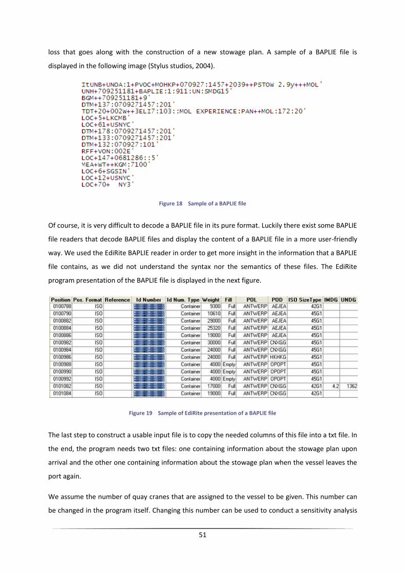
51
loss that goes along with the construction of a new stowage plan. A sample of a BAPLIE file is
displayed in the following image (Stylus studios, 2004).
Figure 18 Sample of a BAPLIE file
Of course, it is very difficult to decode a BAPLIE file in its pure format. Luckily there exist some BAPLIE
file readers that decode BAPLIE files and display the content of a BAPLIE file in a more user-friendly
way. We used the EdiRite BAPLIE reader in order to get more insight in the information that a BAPLIE
file contains, as we did not understand the syntax nor the semantics of these files. The EdiRite
program presentation of the BAPLIE file is displayed in the next figure.
Figure 19 Sample of EdiRite presentation of a BAPLIE file
The last step to construct a usable input file is to copy the needed columns of this file into a txt file. In
the end, the program needs two txt files: one containing information about the stowage plan upon
arrival and the other one containing information about the stowage plan when the vessel leaves the
port again.
We assume the number of quay cranes that are assigned to the vessel to be given. This number can
be changed in the program itself. Changing this number can be used to conduct a sensitivity analysis
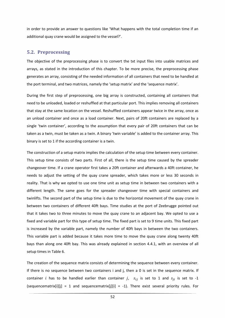
52
in order to provide an answer to questions like ‘What happens with the total completion time if an
additional quay crane would be assigned to the vessel?’.
5.2. Preprocessing
The objective of the preprocessing phase is to convert the txt input files into usable matrices and
arrays, as stated in the introduction of this chapter. To be more precise, the preprocessing phase
generates an array, consisting of the needed information of all containers that need to be handled at
the port terminal, and two matrices, namely the ‘setup matrix’ and the ‘sequence matrix’.
During the first step of preprocessing, one big array is constructed, containing all containers that
need to be unloaded, loaded or reshuffled at that particular port. This implies removing all containers
that stay at the same location on the vessel. Reshuffled containers appear twice in the array, once as
an unload container and once as a load container. Next, pairs of 20ft containers are replaced by a
single ‘twin container’, according to the assumption that every pair of 20ft containers that can be
taken as a twin, must be taken as a twin. A binary ‘twin variable’ is added to the container array. This
binary is set to 1 if the according container is a twin.
The construction of a setup matrix implies the calculation of the setup time between every container.
This setup time consists of two parts. First of all, there is the setup time caused by the spreader
changeover time. If a crane operator first takes a 20ft container and afterwards a 40ft container, he
needs to adjust the setting of the quay crane spreader, which takes more or less 30 seconds in
reality. That is why we opted to use one time unit as setup time in between two containers with a
different length. The same goes for the spreader changeover time with special containers and
twinlifts. The second part of the setup time is due to the horizontal movement of the quay crane in
between two containers of different 40ft bays. Time studies at the port of Zeebrugge pointed out
that it takes two to three minutes to move the quay crane to an adjacent bay. We opted to use a
fixed and variable part for this type of setup time. The fixed part is set to 9 time units. This fixed part
is increased by the variable part, namely the number of 40ft bays in between the two containers.
This variable part is added because it takes more time to move the quay crane along twenty 40ft
bays than along one 40ft bay. This was already explained in section 4.4.1, with an overview of all
setup times in Table 6.
The creation of the sequence matrix consists of determining the sequence between every container.
If there is no sequence between two containers i and j, then a 0 is set in the sequence matrix. If
container has to be handled earlier than container , is set to 1 and is set to -1
(sequencematrix[i][j] = 1 and sequencematrix[j][i] = -1). There exist several priority rules. For
53
example, the sequence due to the hatch covers implies that all unload containers above deck have to
be handled earlier than all unload below-deck containers of the same bay. It is the other way around
for all on-deck load and all below-deck load containers of the same bay.
5.3. Heuristics
Optimising a parallel machine scheduling problem includes two major subproblems. First of all, there
is the job-to-machine assignment, in this thesis the container-to-quay crane assignment. The second
subproblem is determining the sequence of jobs on every machine, in this thesis the container
sequence per quay crane.
The array, constructed during preprocessing, including all containers that need to be handled,
consists of 3566 containers in our initial dataset. If there is only one quay crane assigned to this
vessel, there would be 3566! possible sequences. As can be noticed, the problem we are facing is a
large combinatorial problem. Therefore, some simplifications need to be made. The proposed
solution approach to solve this problem goes as follows. First of all we attempt to determine the
optimal sequence of containers within every bay. To solve this subproblem, some heuristics were
created, explained in the next sections. Once the optimal or near-to-optimal container sequence per
bay is determined, a given number of quay cranes can be assigned to the bays or part of the bays.
Our methodology to solve this container-quay crane assignment problem is explained in the last
paragraph. Of course, this methodology takes into account crane interference and the sequence
between containers.
The next paragraph starts by explaining the current way of dealing with the problem. We
implemented the currently applied methodology in Java. The proposed heuristics try to minimize the
completion time of every bay, by increasing the double cycles and minimizing the total number of
incurred setup times. The results of these heuristics can then be benchmarked against the
completion time of the current practice.
5.3.1. Current way of working
5.3.1.1. Method explanation
This heuristic imitates the current way of loading and unloading of container vessels in port
terminals. By implementing this methodology, the total completion time of a bay can be obtained,
according to the current practices. The calculated result can be very useful to benchmark the
upcoming heuristics and consequently to analyze their performance.

54
The current way of handling container vessels goes as follows. First of all, all containers that need to
be unloaded are unloaded, after which all containers that need to be loaded are being loaded.
Consequently, no dual loops occur. Unloading the containers happens in a special way. Every tier is
unloaded from the quayside towards the waterside. Loading containers happens the other way
around. To be more precise, every tier is loaded from the waterside towards the quayside (Meisel &
Wichmann, 2010; Wyngaert, 2011). This way of loading and unloading a container vessel was already
explained in sections 2.5.1 and 2.5.2, respectively. Terminal operators use this methodology because
it increases the efficiency of the crane operator. It is easier for the crane operator to load a container
when he can put this container in front of a container of the same tier, the crane operator lets the
container slide against the previously placed container. In this way, each container serves as a
guidance to perfectly fit the next container in place. Putting the container behind a container of the
same tier is more difficult because this limits his vision. The same theory justifies the unloading
methodology. Of course, this methodology makes dual loops impossible. Therefore, there is some
time loss, because the empty quay crane spreader has to return to his previous position in order to
take the next container.
The created heuristic acts according to the previously explained methodology. If there are containers
that need to be unloaded, it starts by looking at the highest tier of the bay. Next, it selects the
container in this highest tier with the highest even row number (quayside). If there are no containers
with an even row number, it selects the container in this highest tier with the lowest odd row
number. When the highest tier is finished, the heuristic continues the procedure in a lower tier. After
unloading all the containers that need to be unloaded, the heuristic continues with loading
containers in the lowest tier. First of all, it selects the containers with the highest odd row number,
being containers positioned at the waterside. If all containers in that tier with an odd number are
loaded, the container with the lowest even number will be selected. If the tier is finished, the
heuristic goes on with loading the next, higher tiers until the bay is finished.
5.3.1.2. Results
In order to show the performance and outcome of the heuristics, one representative bay is selected.
In this case, bay 1 is chosen because this bay consists of several load and unload containers that are
located on-deck, as well as several load and unload containers that are located below-deck. In total,
bay 1 consists of 174 containers that need to be handled at the port. This number is a little bit higher
than 162, the initial dataset’s average number of containers per bay.
A part of the output of this heuristic is displayed below in Figure 20. The complete output can be
found in Annex 10.6. This solution method sequences the containers of the bay following the

55
methodology mentioned in the section just-above. Once the container list is generated, a
construction list is generated as well. This construction list determines what the crane, assigned to
bay 1, is doing during every time unit. Consequently, the length of this construction list determines
the total completion time of the bay, taking into account load/unload times and setup times. A
sample of the construction list is given in Figure 21 below.
Figure 20 Output of the current way of working heuristic
Figure 21 A sample of the construction list of the previously generated container sequence of bay 1
The length of this construction list is 743 time units. This completion time can be benchmarked
against the results, obtained when using the heuristics presented in the following sections.
56
5.3.2. Greedy heuristic
5.3.2.1. Method explanation
The search for a heuristic that reduces the current completion time, starts with a greedy algorithm. A
greedy algorithm means that at each decision point the locally optimal choice is made, hoping that
the overall solution will eventually be the global optimum. However, since the applied decision rule
at each stage does not take into account the possible combinations after the next stage, this is
mostly not the case. The biggest advantages of greedy algorithms are that they are able to find a
solution very quickly and that they are rather easy to implement. This means that a greedy algorithm
can be very useful for problems with a large number of possible combinations, like this parallel
machine scheduling problem.
The decision rule used within the greedy heuristic is explained in this paragraph. At each stage, the
heuristic adds a container, that has the minimum combination of setup and idle time with the
previously assigned container, to the solution. This container needs to satisfy two conditions. First of
all, the priority rules concerning this container must be respected. This means that it must be
possible to handle this container, taking into account the sequence rules. Secondly, the container
cannot be part of the solution already. The first container that is added to the solution, is the first
container of the array that satisfies the first condition. At every stage, all containers of the bay are
evaluated regarding these conditions after which the heuristic selects the best possible solution.
5.3.2.2. Results
Thanks to this heuristic the completion time drops from 743 to 692 time units. This is a time gain of
51 time units for bay 1. The decrease in completion time is largely caused by the drop in total setup
time between consecutive containers. The other part of the decrease in completion time is due to
the drop in idle time, caused by scheduling dual loops instead of single loops.

57
Figure 22 Output when using the greedy heuristic

58
5.3.3. GRASP
5.3.3.1. Method explanation
Mostly, a greedy heuristic is not able to find the global optimum, as explained earlier. It is limited
because it looks only one step further. A heuristic that looks several steps further, is able to
overcome short sighted problems. Consequently it can give a semi-local optimum. Therefore, it is
opportune to take a look at such a heuristic. The large number of containers makes it difficult to
explore all possible combinations in the neighbourhood of one stage. As a result, GRASP could be a
good methodology to provide a better solution to this problem.
GRASP stands for Greedy Randomized Adaptive Search Procedure. GRASP is a multi-start or iterative
procedure where each GRASP iteration consists of a construction phase, where a feasible solution is
constructed, followed by a local search procedure that aims at finding a locally optimal solution
(Resende, 1998). This means that such a heuristic randomly picks out several possible feasible
solutions and tries to improve them by applying local search methods. The main advantage of this
heuristic is that it looks several steps further in order to add an element to the solution. The most
important drawback is that it does not take into account all possible solutions, because of the
randomly picking of possible solutions. That is why it is possible that the neighbourhood of the
optimal solution is not explored. Of course it is not efficient to explore all possible solutions, as this
requires too much computation time.
In this paper, a variant of GRASP is created to solve the parallel machine scheduling problem. The
heuristic constructs several possible combinations of 5 containers, taking into account the sequences
between the containers. The first container of these combinations is the last container of the
constructed solution. For the second container, five feasible containers are randomly picked. For
each of these second containers, again five possible containers are picked to be the next container.
The same goes for the fourth container. In total, 5x5x5x5 or 625 possible combinations are explored.
The combination with the lowest completion time is retained. The four containers of the best
combination are added to the solution. This heuristic could find a better solution to the parallel
machine scheduling problem than the greedy heuristic, by limiting the short sightedness of the latter
heuristic. By looking several stages further, the variant of GRASP should be able to increase the
number of dual loops and reduce overall setup time significantly. The procedure of the variant of
GRASP is explained in the next figure.

59
Figure 23 GRASP variant
5.3.3.2. Results
The results of the newly designed heuristic are disappointing, although the heuristic indeed assigns
more dual loops than the greedy heuristic. However, the time gain caused by the higher number of
dual loops merely accounts for two time units. Furthermore, the total setup time is not being
optimised at all. When using this heuristic, the overall setup time is 25 time units higher than the
greedy heuristic. Consequently, the total completion time for the variant of the GRASP takes 23 time
units more than the greedy heuristic. Additionally, another big problem is the high computation time.
A sample of the output is provided in Figure 24.

60
Figure 24 Result of variant on GRASP
As can be derived from the results, the GRASP method has two main drawbacks. The first one is that
the number of variables becomes larger when the problem size becomes larger, thus increasing the
problems’ complexity. As this entails higher computation time, this GRASP method is only applicable
to small-sized problems. The enormous computation time and computer-memory requirements
associated with GRASP methods limits their application to large problems. As can be observed in
Figure 24, the GRASP method needs 282 minutes in order to schedule the 174 containers of bay one.
The second weakness of the GRASP method is that it does not always pick the optimal combination
in the neighbourhood of the already constructed solution. Because of the randomly picking of
possible combinations, the solution space around the local optimal solution is not always explored. In
the output it becomes clear that too many changes between 40ft and 20ft containers occur. This is
probably due to the weakness of the randomly picking technique.
5.3.4. Intelligent constructive heuristic
5.3.4.1. Method explanation
It is obvious that previous heuristics can be improved. First of all, the number of dual loops must
further be increased in order to decrease the completion time. On the other hand, this may not be at
the expense of the computation time. Therefore an intelligent constructive heuristic, that optimises
the number of dual loops, is designed. This heuristic adds elements to the solution, while using
several decision rules.
Given the list of containers of a bay, the heuristic starts by checking the location of all containers. To
be more precise, the heuristic investigates whether there are unload or load containers on-deck and

61
whether there are unload or load containers below-deck. Depending on the result of this verification,
the sequence of the next actions is determined. Imagine that there are unload and load containers
both on-deck as well as below-deck. In this case, the heuristic states that first of all the unloading of
the unload containers on-deck needs to be optimised, after which the optimisation of dual loops
below-deck needs to take place and finally the loading of the containers on-deck has to be optimised.
In total, there are 4² or 16 possible solution structures of a bay, which can be translated into four
binary variables. All possible combinations with their resulting actions are shown in Figure 25 below.
Determining the specific actions that need to be taken, aims at reducing computational effort and
resulting computation time.
Figure 25 The possible solution structures for a bay
This heuristic applies two types of solution methods to execute the previously determined actions.
When an action concerns loading or unloading a part of the vessel and no dual loops can occur, the
greedy heuristic, that is explained in section 6.3.2, is used to determine the solution for the
corresponding part of the bay. This heuristic adds the container that has the minimal setup time with
the container that was previously assigned to the solution. This decision rule is applied on this type of
actions, because the greedy heuristic provides a near-to-optimal solution in cases where no dual
loops are possible. Afterwards, local search methods can be applied to improve the constructed
solution, if possible.
If an action implies the optimisation of dual loops in a part of the vessel, another procedure is used
to construct a solution. In that case, all rows that contain unloading as well as loading containers are
listed in an array, the so-called ‘samerows’ array. At the first stage, the heuristic starts by unloading a
container that is located in the row number corresponding to the first element of the array, taking
into account the sequence constraints. Whenever possible, a load container is alternated with an
unload container in order to optimise the number of dual cycles. When there are no more containers
in the row number corresponding to the first element of the array, the heuristic skips to the next

62
element of the array. When the array is finished, unload containers with other row numbers are
taken into consideration.
5.3.4.2. Results
The results verify that implementing the intelligent constructive heuristic entails significant
improvements as compared to previous heuristics. The drop in idle time is caused by the
implementation of dual loops. On the other hand, total setup time is relatively high, which is caused
by forcing the implementation of these dual loops. Processing time is negligible (less than 40
seconds), thanks to the subdivision in actions, as described in section 5.3.4.1. The resulting output is
partially displayed in Figure 26. The complete output can be found in Annex 10.8.
Figure 26 Sample of output of intelligent constructive heuristic
First of all, the heuristic looks at the location of the containers (check upperdeckunload, … ). It uses
this information to determine the sequence of actions. An optimisation of below-deck dual loops is
needed in bay one after the unloading of the containers located on-deck. Therefore, an array is
constructed with the below-deck row numbers in which both unload and load containers appear. The
first row number, satisfying this condition is row number nine. As can be seen in the solution,
unloading indeed starts in this row. The next row is being unloaded when the unloading of the first
row is finished.

63
5.3.5. Local search improvement heuristics
5.3.5.1. Method explanation
Previous solutions can be optimised using local search heuristics. Two types of improvement
heuristics are designed. The first one swaps two containers in the constructed container list. If the
sequence constraints are respected and if the changed container list has a lower completion time,
the old solution is replaced by the new solution. The second local search heuristic does not swap two
containers in the list, but simply takes one container and puts it somewhere else in the list. Again, if
the sequence is respected and the changed container list has a lower completion time, the previous
solution is replaced by the new solution.
5.3.5.2. Results
When the combination of the local search heuristics is applied to the intelligent constructive
heuristic, only small improvements can be noticed. They reduce the completion time of bay one from
672 to 670. The computational effort needed for these improvement heuristics is limited. Only three
minutes are needed to improve the solution of bay one. When the heuristics are applied to the
solution of the greedy algorithm, the completion time is reduced from 692 to 691.
As a result, it can be concluded that these local search heuristics provide only incremental
improvements, though within a reasonable computation time.
5.3.6. Intelligent constructive heuristic with randomized extension
5.3.6.1. Method explanation
The previous intelligent constructive heuristic can be improved. When dual loops are possible, the
heuristic starts picking unload containers from the row number that is equal to the first element of
the constructed ‘samerows’ array. When all containers of that row are handled, it skips to the next
element of the array. The sequence of elements in that ‘samerows’ array is not optimised. The
results show that the setup time is relatively high. Therefore it might be opportune to shake up the
elements of the array several times and afterwards pick the array that leads to the lowest completion
time. This methodology can decrease the setup time by scheduling rows with the same type of
containers in a consecutive order.
The structure of this heuristic is similar to the structure of the previous heuristic. The heuristic
presented in this section includes only two differences with respect to situations where dual loops
are possible, as compared to the initial intelligent constructive heuristic. In this case, the ‘samerows’
array is constructed, after which a new array is constructed by randomly inserting the elements of
this ‘samerows’ array. Afterwards, the completion time of this part of the bay is calculated, using the

64
new array. New ‘samerows’ arrays are created in this way and their corresponding completion times
are measured during a number of iterations. This number of iterations is set to
or to , in order to take into account the size of
the array. The second difference consists of a local search that is executed on the best random
solution that has been found. The number of iterations of this local improvement is set to
. During each iteration, two different elements of the ‘samerows’ array are
randomly selected and their positions are swapped. If the fitness value – namely the completion
time – of the new array is better than the fitness value of the previous best solution, the new array
replaces the best solution. Mostly, several local improvements can be made by using these swaps.
When no dual loops are possible, the heuristic follows the methodology of the previously explained
heuristic.
5.3.6.2. Results
The results verify that the intelligent constructive heuristic with random extension is a significant
improvement compared to intelligent constructive heuristic. The decrease in total completion time
for bay 1 amounts only 4 time units. Furthermore, the improvements in the other bays are displayed
in the following table. The bays, where no dual loops are possible, are not included in this table,
simply because no improvements are made in these bays when using the new heuristic.
Table 10 Comparison of results
The table above shows that the random extension improves the previous heuristic. Especially in bays
where there is a large variety of types of containers, like bay 7, 10, 13 and 16, significant
improvements can be noticed. Of course it takes computational effort to shuffle the elements of the
array and to calculate the corresponding completion time. Therefore we displayed the results both
when the number of iterations is set to , as well as to
. When increasing the number of iterations, the improvements
are better. On the other hand, increasing the number of iterations causes a drastic raise in
computation time. This comes down to a trade-off between improvements and computation time.
When local search is executed on both best found solutions, it becomes clear that it is not
worthwhile to set the number of iterations to . The end result is
more or less the same when using a different number of iterations. Sometimes it occurs that the end

65
result is even better when less iterations are used. This is because the local search method can find
bigger improvements. In the next sections it is assumed that the constructive heuristic with
randomized extension uses a number of iterations that is equal to
and a local search method that is applied to the best solution
found.
5.3.7. Hybrid genetic algorithm
5.3.7.1. Genetic algorithm
A genetic algorithm is a population-based, evolutionary algorithm. It tries to find a good solution by
combining parent solutions in order to construct a ‘child solution’ or an offspring. Although a genetic
algorithm does not ensure an optimal solution, it provides good approximations within a reasonable
computation time, as compared to exact algorithms. It is currently a prominent and widely used
method for solving combinatorial optimisation problems. In particular, the following steps are
important:
Encoding of the problem into proper chromosomes
In a genetic algorithm, solutions are represented using chromosomal encoding. For the QCSP,
a natural way to represent its solution is through a sequence of operations, as it is for many
scheduling problems. For example, chromosome [1 2 3 4 5 6 7 8], could indicate the
handling sequence 1 2 3 4 5 for QC1, as well as the sequence 6 7 8 for QC2.
In this chromosome, numbers 1 until 8 obviously represent containers to be handled by the
quay cranes. However, in the presented solution method, container sequencing and QC
assignments are worked out separately, while only representing the container sequences per
bay using chromosomes, as follows: [1 2 3 4 5]. This chromosome once more indicates a
handling sequence 1 2 3 4 5, though for containers 1 until 5 of one and the same
bay. Afterwards, QCs will be assigned to handle these containers, according to the proposed
sequence.
Genetic operators: crossover, mutation and selection
- Crossover operator
Recombination plays a crucial role in the performance of Genetic Algorithms. As with the
natural selection principle, the aim of a GA is to transfer important information existing in
the parents, to their offspring. In the case of the QCSP, a precedence preserving crossover
should be used, passing on the parents’ precedence relations to the offspring, without

66
introducing new precedence relations. An explanation on the crossover operators, used
within this solution method can be found below.
- Mutation operator
In general, mutation operators should alter a permutation only slightly (Hui, Dong, &
Guanghong, 2008). The most commonly used mutation operators are Insert operators,
Inversion and Swap mutation operators. An example on a Insertion mutation operator can
be found in below:
Figure 27 Insertion mutation operator
- Selection operator
New offspring created by genetic operators – namely the crossover and mutation
operators mentioned above – may be infeasible solutions, even though both parents are
feasible. Since offspring is used to generate a new population, precedence relations
should be evaluated before solutions are embraced into the population. Infeasible
chromosomes should be rejected directly, increasing the total performance of the
population, as well as computation efficiency. Furthermore, decision rules should be
determined, that state which solutions to take into the new population. While it seems
logical only to take improved solutions into the new population, also worse solutions are
often selected, in order to diversify the population.
Defining a fitness function, in order to evaluate the performance of resulting solutions
(offspring chromosomes)
The fitness function merely has to check the quality – and eventually also the feasibility – of
the obtained solution. This is easily done by evaluating the proposed solution using the
objective function. Frequently, this fitness function is used to perform the selection
operation, often only selecting the solutions with the highest fitness value.
These GA ‘building blocks’ are then used in a certain method architecture, which will further be
discussed in the next section.
Chrom: 1 2 3 4 5 6
1 2 3 4 * 5 6
New Chrom: 1 3 4 2 5 6

67
5.3.7.2. Hybrid genetic algorithm: method explanation
A hybrid genetic algorithm consists of a combination of a genetic algorithm and another search
procedure. This hybrid genetic algorithm approach uses the solutions of both the intelligent
constructive heuristic with randomized extension as well as the greedy heuristic as initial solution.
This is done in order to reduce the search space and computation time.
A genetic algorithm is created in order to optimise the sequence of containers in a bay. It starts by
creating randomly two hundred feasible solutions. Afterwards, an elite list of the twenty-five best
solutions is constructed by evaluating the completion time of the random solutions. The first elite list
consists of the 23 best found random solutions, as well as the solution from the greedy heuristic and
the solution from the constructive heuristic with randomized extension. Starting from this top
twenty-five list, a first cycle is initiated. A cycle consists of several steps. The objective of a cycle is to
create 4000 offsprings out of the twenty-five best solutions. This is done by randomly picking twenty
couples of parent solutions from the elite list. Each couple is recombined a hundred times in order to
produce hundred offsprings out of one couple. The recombination method is explained in the next
paragraph. In total, 2000 offsprings are created at this stage of the cycle. Next, a mutation method is
used on each offspring in order to create extra offspring. The used mutation methods are explained
in section 5.3.7.4. Afterwards, the fitness value of each offspring is measured and it is verified
whether or not the sequence of the containers in the new list is consistent with the sequencing rules.
Remind that, in this parallel machine scheduling problem, the fitness value corresponds to the
completion time of the list of containers. If an offspring is not a copy of an existing solution in that
elite list and if that offspring has a lower completion time than the worst solution in the elite list, this
worst solution is eliminated out of the top twenty-five list and the offspring is inserted. After the
update of the top twenty-five list at the end of each cycle, the eight worst solutions are deleted from
the array and eight random, feasible solutions are inserted. This is done in order to avoid rash
convergence and to increase the diversity of solutions in the top ten list. Afterwards a new cycle
begins. This heuristic is a good methodology to search an optimum in the neighbourhood of a
solution, but the main drawback is that it can lead to premature convergence. Therefore, the
solutions of the greedy heuristic and the intelligent constructive heuristic with randomized extension
are added to the elite list during the first iteration. This heuristic optimises the sequence of loading
and unloading the rows of a bay. Consequently, it provides a good direction for the global optimum.

68
Figure 28 The methodology of the hybrid genetic algorithm
5.3.7.3. Recombination methods
Creating an offspring requires a recombination method. The method used in this genetic algorithm
needs two parent solutions to produce an offspring. First the offspring is initialized as a copy of the
first parent solution. In the next step, the length of the recombined part is randomly chosen between
3 and 20. Also the index, where the recombination starts, is randomly chosen. Imagine that the
length is 5 elements and that the index is 0. In that case, the heuristics memorizes the first five
elements of the first parent solution. Next, it looks at the sequence of these five elements in the
second parent solution and implements this sequence of the five elements in the offspring list on the
first five indices. The recombination method is explained graphically in the next figure.
Figure 29 Example of the recombination method (length = 5; index = 0)
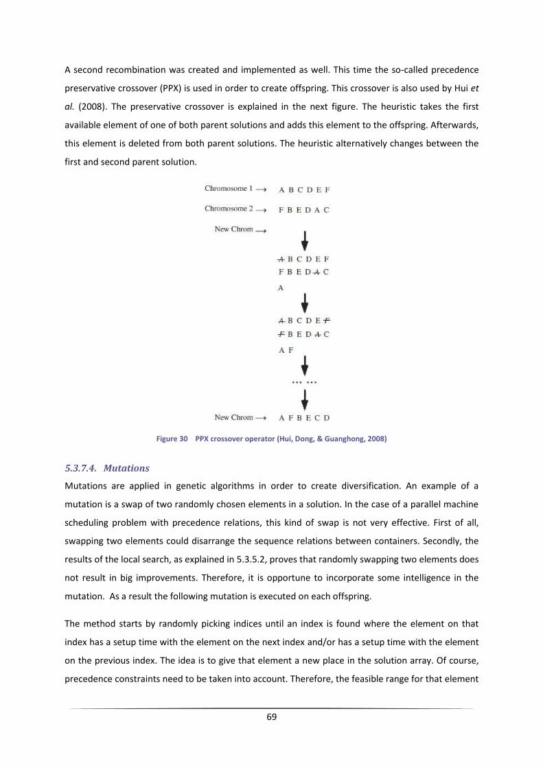
69
A second recombination was created and implemented as well. This time the so-called precedence
preservative crossover (PPX) is used in order to create offspring. This crossover is also used by Hui et
al. (2008). The preservative crossover is explained in the next figure. The heuristic takes the first
available element of one of both parent solutions and adds this element to the offspring. Afterwards,
this element is deleted from both parent solutions. The heuristic alternatively changes between the
first and second parent solution.
Figure 30 PPX crossover operator (Hui, Dong, & Guanghong, 2008)
5.3.7.4. Mutations
Mutations are applied in genetic algorithms in order to create diversification. An example of a
mutation is a swap of two randomly chosen elements in a solution. In the case of a parallel machine
scheduling problem with precedence relations, this kind of swap is not very effective. First of all,
swapping two elements could disarrange the sequence relations between containers. Secondly, the
results of the local search, as explained in 5.3.5.2, proves that randomly swapping two elements does
not result in big improvements. Therefore, it is opportune to incorporate some intelligence in the
mutation. As a result the following mutation is executed on each offspring.
The method starts by randomly picking indices until an index is found where the element on that
index has a setup time with the element on the next index and/or has a setup time with the element
on the previous index. The idea is to give that element a new place in the solution array. Of course,
precedence constraints need to be taken into account. Therefore, the feasible range for that element

70
is constructed by checking the precedence relations with elements in the neighbourhood of the
chosen index. In the final step, the element is given a new index within the feasible range. This way a
new, feasible solution is constructed. Two possibilities to give the element a new place in the feasible
range are examined. The first one is to pick randomly an index within the feasible range. The other
option is to pick randomly indices until an index is found where the setup time with the next and
previous element is lower than the incurred setup time at its initial position.
In total, four mutations are possible. They are listed in Figure 31 below.
Figure 31 The four examined mutation methods
5.3.7.5. Results
The results of the second recombination method, using the precedence preservative crossover, are
disappointing. A lot of feasible offsprings are generated, but none of them improve the initial
solutions of the greedy algorithm and the constructive heuristic with randomized extension.
Therefore, this recombination method is not used in the presented genetic algorithm. In contrast,
the first recombination method proves to be efficient and is able to improve the initially generated
solutions. Consequently, only this recombination method is used in the hybrid genetic algorithm.
As discussed in 5.3.7.4, four mutations are tested. Test are executed on the two bays where most
improvements are possible, namely bay 7 and bay 10. The four mutations are applied separately in
the genetic algorithm, during the first four tests. In the fifth and last test, the four mutations are used
altogether in the hybrid genetic algorithm. In this case, when a mutation offspring has to be created,
one of the four mutations is randomly picked and applied on the previously constructed offspring.
The test result are displayed in Table 11. The displayed improvements per bay are the average of
three test runs. The best results per measure are presented in bold.
Table 11 Test result for four mutations (average improvements per bay are displayed)

71
The results show that two mutations are very promising. The first one is the mutation that picks an
element that has setup time with the previous and/or next element. This element is placed on an
index where it has a lower setup time than the initial setup time. This mutation gives the best results.
The second mutation with decent results is the one that picks an element that has setup time with
the previous and the next element and places that element randomly within the feasible range. The
results for the method that randomly picks one of the four mutation methods, are also positive.
Because these tests are based on only 6 instances and because the final completion times are not
always the same, these three best mutation methods are examined in more detail. This time using 20
instances in total. Using more instances should allow to draw better conclusions. The test results of
the three most promising mutation methods, as well as the combination of the two separate
mutations, are shown in Table 12.
Table 12 Test results for most promising mutations (average improvements per bay are displayed)
The results of these promising mutation methods are quite close. However, the first mutation causes
the biggest improvements in both bays. Therefore, it is preferred to use this mutation in the hybrid
genetic algorithm.
A test is executed in order to measure both the effectiveness of the recombination method, as well
as the effectiveness of the mutations. As the mutations increase CPU time drastically, it is opportune
to verify whether their impact on the results are significant. Therefore, the results of the hybrid
genetic algorithm without mutations are examined. The tests are executed on data of five vessels.
The average improvements over the result of the constructive heuristic with randomized extension
are displayed for every vessel in Table 13. The improvements for the hybrid genetic algorithm with
mutations are significantly higher than those for the hybrid genetic algorithm without mutations.
Therefore, the mutations are added to the hybrid genetic algorithm.
Table 13 The average improvement over the extended constructive heuristic for the hybrid genetic algorithm with and without mutations

72
A sample of a possible best found solution of the hybrid genetic algorithm for bay seven is displayed
in Figure 32. The left part of the figure displays the outcome of the constructive heuristic with
randomized extension. This solution is transformed by the hybrid genetic algorithm. The result of the
latter heuristic is shown in the right part of the figure.
Figure 32 Evolution between solution of constructive heuristic with randomized extension (= input for hybrid genetic) and solution of hybrid genetic
5.3.8. Intermediate solution
5.3.8.1. Method explanation
A limitation of the model is that the distance between two rows is not taken into account. This might
cause an error when forecasting the time gain caused by dual loops. This can be explained by an
example. Imagine that a dual loop is scheduled. A first container is loaded in row 18, at the quayside.
Afterwards, a container in row 19 is unloaded. In that case, the spreader has to move towards the
other side of the ship, from quayside to waterside, in order to pick up the second container. This
way, a fraction of the time gain of the dual loop is lost. Figure 33 explains graphically this type of time
loss. Our model does not take into account this distance between rows, since it assumes that the
time gain of executing a dual loop is always the same.

73
Figure 33 Time loss due to distance between containers in dual loop
A possibility to deal with this problem is to sequence the elements of the ‘samerows’ array in the
constructive heuristic from quayside to waterside. On one hand, this sequence neglects the
optimisation of the setup times between containers. On the other hand, this sequence does minimize
the distance between containers that need to be handled. It is difficult to estimate the time losses
because of the extra distance the spreader has to make. Therefore, we can recommend this problem
as a topic for future research.
5.3.8.2. Results
Figure 34 Intermediate result for bay 1

74
Figure 34 displays part of the results for bay 1. The elements of the ‘samerows’ array are sequenced
from quayside to waterside. The time loss for this bay when using this method is marginal. Total
completion time increases from 668 to 770. Consequently, this solution might be better than the
solution of the constructive heuristic with randomized extension, because it minimizes spreader
movement time. However, using this heuristic on other bays where dual loops are possible, can
sometimes dramatically raise completion time. A good example of this phenomenon is bay 7, where
completion time increases from 1258 (constructive heuristic with randomized extension with local
search) to 1320 because of the sharp increase in setup time.
5.3.9. Container crane assignment methodology
5.3.9.1. Method explanation
The previously explained heuristics are designed to optimise the first sub-problem of the parallel
machine scheduling problem. They optimise the sequence of containers within every bay. The second
sub-problem consists of determining which quay crane will handle which containers. This is called the
container-quay crane assignment problem. This section gives information concerning the
methodology used to solve this problem.
The main assumption that is made concerns the movement direction of the quay cranes. These quay
cranes are assumed to work from the vessel’s fore to aft. This assumption can be justified by two
arguments. The first reason is that the corresponding handling sequence of bays reduces the total
completion time for the quay crane by limiting the overall setup time. Imagine a quay crane has to
handle bay one, two and three. If the crane finishes the bays in the assumed sequence (1 2 3),
the total setup time for the crane will be lower than when the crane handles the bays in another
sequence, let’s say first bay one, then bay three and finally bay two. This is due to the variable part of
the setup time resulting from the movement of the quay crane along the quay, when moving from
one bay to another. This variable part takes into account the distance between two bays. The second
argument is that such sequence is more likely to avoid crane interference. When all quay cranes
move into the same direction, the chance of interfering each other’s safety zone is evidently
minimized.
This thinking pattern is implemented in the Java program. First, the optimised completion times of all
bays are summed. Next, this total is divided by the number of assigned quay cranes in order to
calculate the average workload per quay crane. Afterwards, consecutive bays are assigned to a quay
cranes until the average workload per cranes is exceeded. In order to come into the neighbourhood
of this average it is often necessary to split a bay. A bay split consists of assigning a part of a bay to

75
the first quay crane and the other part to the next crane, taking into account the sequence rules. This
results in a better, but not optimised balance of the workload per quay crane. Therefore, a balancing
method is designed. This balancing method balances the workload of two consecutive quay cranes by
transferring containers from the crane with the highest workload to the crane with the lowest
workload. This method is applied on all consecutive quay cranes during several iterations in order to
obtain an optimal overall balance.
A scenario analysis can be obtained by using different numbers of assigned quay cranes and
comparing the results. This way, it is possible to compare the overall completion time of the
container vessel when less or more quay cranes are assigned to the vessel, by taking a look at the
workload of the quay cranes.
5.3.9.2. Results
The results of applying the intelligent constructive heuristic and local search heuristics is shown in
the next figure. The assigned number of quay cranes totals three.
Figure 35 Result for three quay cranes when using the intelligent constructive heuristic and local search heuristics
5.4. Results
Above, the implemented solution methods were presented and compared, using one single data set.
This section will discuss the overall effectiveness of the solution methods, based on five different
data sets. In order to do so, we have obtained BAPLIE files from 5 different vessels, both an arrival as
well as a departure configuration of each vessel. In the smallest dataset, 441 containers have to be
handled, whereas the largest numbers of containers to be handled amounts 3566. The results for the
different solution methods are presented in the table below:
Table 14 Efficiency gains for different datasets
Total containers
Total Improve Total Improve Total Improve Total Improve Total Improve
(TUs) (%) (TUs) (%) (TUs) (%) (TUs) (%) (TUs) (%)
Current way of working 8.084 2.941 1.810 2.177 14.589
Greedy heuristic 7.478 7,50% 2.753 6,39% 1.664 8,07% 2.045 6,06% 13.818 5,28%
Constructive heurstic 7.419 8,23% 2.754 6,36% 1.652 8,73% 2.030 6,75% 13.762 5,67%
Extended constructive heuristic 7.352 9,05% 2.754 6,36% 1.639 9,45% 2.012 7,58% 13.689 6,17%
Hybrid genetic algorithm 7.322 9,43% 2.718 7,58% 1.627 10,11% 1.998 8,22% 13.639 6,51%
Vessel 4
532
Vessel 5
3.5661.941
Vessel 1 Vessel 2
714
Vessel 3
441

76
From the table we can clearly conduct that the proposed hybrid GA yields the best results, and is
fairly stable over the different datasets. Note that all improvements are calculated in relation to the
current way of working. Only for vessel 2, there is an inconsistency in the results, as compared to the
improvements for all other vessels. In this case, the greedy heuristic results in a bigger improvement
than both the constructive, as well as the extended constructive heuristic. Since both constructive
heuristics force double cycling, without taking setup times into account, this results in only little
improvements in this particular case. This is due to the fact that, for this particular vessel, unloading
and loading containers often have different dimensions, inevitably resulting in high setup times.
Consequently, it only makes little difference whether to use the greedy or the intelligent constructive
heuristics. As the matter in fact, only in two out of seven bays of vessel 2 the constructive heuristics
are outperformed by the greedy heuristic.
Accordingly, we can take a look at the relationship between the number of samerows13 in a vessel
and the resulting QCSP solutions. Since working with total handling times would be irrelevant in this
case, results are displayed as average handling time per container. The scatter diagram can be found
below:
Figure 36 Relationship between the number of samerows and CPU time per container
13
Rows in a vessel that both need unloading, as well as loading actions

77
This plot confirms the presumptions that double cycling indeed increases quay crane container
handling efficiency. On average, the more samerows in a certain bay, the lower the average handling
time required per container.
Next, statistical analysis points out that there is a positive correlation between the number of
containers per bay and the CPU time required to execute the hybrid genetic algorithm. When the
number of containers increases, the CPU time increases slightly more than proportionally. This is
logic because the constructed solutions and offsprings contain more elements. Consequently, all
tasks performed on these solutions and offsprings require more computation time.
Next to this first correlation, the minimum required CPU time increases when the total number of
containers of a vessel increases. This is due to the fact that a large number of containers on a vessel
induces a large sequence and setup matrix. Therefore, more time is needed to perform actions on
these matrices. As a sequence and setup matrix is constructed for an entire vessel, even bays with a
small number of containers can have a fairly high CPU time. The next figures explain these relations
graphically. Vessel five contains more containers than vessel four. Consequently, the intercept with
the y-axis is higher for vessel five.
Figure 37 Effect of the number of containers per bay on the CPU time
The same positive relation is identified between the number of containers per vessel and the total
CPU time required when the hybrid genetic algorithm is used. This is proven by the figure below:

78
Figure 38 The relation between the number of containers per vessel and the required CPU time (for hybrid genetic)
In short, we can state that the proposed solution methods can be used as a practical tool for solving
the CQSP, using a GA that yields considerable improvements. Furthermore, since both the intelligent
and the extended intelligent constructive heuristic to the utmost extent are based on decision rules,
these solution methods’ computation times are rather low. As such, the extended constructive
heuristic can be used as a real-life decision support tool if quick, though qualitatively decisions must
be made. If more time is available, the hybrid genetic algorithm will of course yield a better solution,
though requiring more CPU time.
Furthermore, the obtained results are in line with Goodchild and Daganzo (2007), supposing a
reduction by 25% in the number of crane moves, based on their model, equal to a time reduction of
9,5%. On average, the proposed GA solution method in this paper yields a time reduction of 8,4%.
Number of containers per vessel

79
Chapter 6.
Sensitivity analysis
In the previous chapters, it is assumed that setup time is required between two containers of a
different dimension. This assumption is made because of the fact that the spreader setting needs to
be adapted when taking a container of a different size. This spreader changeover takes more or less
thirty seconds. Therefore, one time unit is used as setup time in order to take into account this time
loss. It is possible that, in the future, new types of spreaders will be developed that perform such a
spreader changeover in only a couple of seconds. As a result, the setup time would be negligible. This
sensitivity analysis shows what happens when the setup time between all containers of the same bay
is set to zero. The results for all vessels are shown below in Figure 39.
Figure 39 Time gain when there is no setup time between containers of the same bay
Obviously, the completion time of each vessel drops because of the fact that there is no more setup
time between containers of the same bay. Another effect is the significantly higher improvement
percentage over the current way of working when setup time becomes negligible. This is due to the
fact that there is a positive correlation between the number of dual loops and total setup time. The
improvements caused by the dual loops are partly neutralized by the higher total setup time.
Consequently, less improvements can be made by scheduling dual loops when setup time is taken
into account. The overall result is that on average, when the spreader changeover time is reduced,
the time gain caused by dual loops will increase.

80
Chapter 7.
The economic point of view
7.1. Financial impact
In this chapter we try to estimate the financial impact of the improvements resulting from the dual
loops. These estimations are based on a paper concerning the economic evaluation of dual loops by
Goodchild and Daganzo (2007). The drop in completion time by executing dual loops has positive as
well as negative financial consequences for several parties involved. In the next figure, the estimated
extra revenues and costs per container handled are shown. The calculations are based on the
assumptions that the improved container handling reduces the vessel completion time by 10% and
that all gained resources are usefully employed. Moreover, it is assumed that a vessel, containing
1500 containers, can be handled in 50 hours using single cycling and within 45 hours using double
cycling. More information on the calculations is given in the next paragraphs.
Table 15 Extra revenues and costs from double cycling
Vessel productivity
A reduction in handling time at the port, gives the vessel the opportunity to increase its
productive time. Consequently, it can use the gained time to transport (other) goods by sea,
resulting in more revenues for the vessel operator. Using the common freight rates, the revenues
for an average vessel can be estimated at $54000 (assuming a 6000 TEU vessel to travel 200 km in
the 5 hours saved). This is a value of $36 per transported container. Also the cost of this gained
transportation time need to be taken into account. It is estimated that the fuel needed to travel
200 km in the 5 hours saved, amounts $20000 or $13,33 per container. The vessel operator is the
benefactor of the gain in vessel productivity.
81
Crane productivity
The cranes can handle all containers of a vessel in less time when using double cycling. Therefore,
the gained time can be used to serve another vessel. Terminals are mostly paid per container
handled. The average rate amounts $200 per handled container. Consequently, it is possible to
generate $33000 within 5 hours. This comes down to $22 per container. The terminal operator
benefits from the increase in crane productivity.
Berth utilization
The vessel operator has to pay two fees in return for berthing space. The first one is the dockage
fee. This fee is paid to the port authority on a daily or hourly basis. As a result, the cost for the
vessel operator decreases, because the vessel stays a shorter period of time at the port. The
revenue of the port authority stays the same, assuming that there is always another vessel
waiting for that berthing space. It is estimated that the dockage fee can be reduced by $2400, or
$1,60 per container handled at the port.
The second fee is the wharfage fee. These wharfage fees are paid on container basis and average
$200 per container. They are paid to the port authority or the terminal operator. This comes
down to a benefit of $22 per handled container.
Other possible revenues and costs
Goodchild and Daganzo (2007) also mention extra revenues thanks to savings landside vehicles
and driver wages, and extra costs due to investments in container handling equipment. We
believe these extra costs and revenues are negligible. The paper states that the straddle carrier
productivity can be increased when dual loops are performed. According to our opinion, this is
not always true and is a function of the yard layout. According to this yard layout, there can be
savings or costs. Therefore, it is not appropriate to include these revenues in the calculations.
Furthermore, Goodchild and Daganzo (2007) state that new container handling equipment is
needed when dual loops are executed. We believe the container handling can be done with the
same equipment as with single cycling. As a result, these costs are left out of the calculations.

82
7.2. Implementation issues
It is obvious that implementing dual cycles has positive overall financial consequences. Now the
question can be posed why double cycling has not been implemented at port terminals. Two main
reasons can be identified. The first one is the diffusion of benefits of double cycling, which results in
reluctance of implementing double cycling. The second issue is the discussion concerning the
productivity of crane operators. These two main problems are described in the following paragraphs.
7.2.1. Diffusion of benefits
As can be derived from Table 15, the gains from double cycling are distributed among the vessel
operator, the terminal operator and the port authority. Therefore, it is a difficult decision for the
terminal operator to make the initial investments for the implementation of double cycling. Three
investments are identified.
The first investment is inevitable. Without this investment dual cycles are not possible. It concerns an
investment in the software used by the straddle carriers. Nowadays a system is used that obliges the
straddle carrier to use one single operational mode: the load mode or the unload mode. When
unloading the entire vessel, the unload mode is used. When all unload containers are moved to the
yard, the mode of the straddle carriers is switched to the load mode. Implementing double cycling
implies an investment in a new software system for the straddle carriers that is able to combine both
modes.
Two additional investments are recommended. First of all, research on the topic of yard planning for
double cycling has to be done. By rescheduling the yard, so that straddle carriers can easily drop
unload containers and pick up load containers, transportation cost can be reduced (as previously
explained in Figure 11). As a result, savings in straddle carrier usage and driver wages could be
possible. A second research topic concerns the link between stowage planning and double cycling. It
is opportune to investigate the additional time gain that can be achieved by optimising the stowage
plan by taking into account the possibility of dual cycles. This way, more dual loops per vessel could
be scheduled. This last research topic can imply an additional investment in the stowage planning
software.
It can be concluded that the diffusion of the benefits slows down the implementation of double
cycling. If a larger portion of the benefits would be allocated to those responsible for its
implementation, we would probably see more widespread use of the technique.
83
7.2.2. Crane operator productivity
Nowadays, most terminal operators are reluctant to implement double cycling, because they believe
that crane operators work more efficiently when using the current container sequencing methods. As
explained in sections 2.5.1 and 2.5.2, loading happens from waterside towards quayside, while
unloading happens in the opposite direction. It is believed that crane operators can work faster using
these sequencing methods. Therefore, it is not clear what the impact of double cycling is when the
different productivity of the crane operators is taken into account. These doubts do not favour the
implementation of the double cycling technique.
84
Chapter 8.
Conclusion and recommendations
8.1. General conclusion
In this master paper, research on the topic of dual cycling in the quay crane scheduling problem is
presented. A clear overview is given of both the practical concerns, as well as the possible benefits
behind double cycling. Given the fact that those benefits are greater with a larger total number of
containers (Goodchild & Daganzo, 2007) and given the current trend towards larger container
vessels, it is worthwhile further investigating this promising technique. In order to demonstrate the
efficiency gains associated with double cycling, a model and corresponding solution methods are
proposed.
This model incorporates many real-life operational issues that are often neglected in existing papers,
such as (sequence dependent) setup-times between individual containers, the presence of hatch
covers and specific double cycling considerations. The model is solved using a good mix of intelligent
decision rules, together with a heuristic optimisation method. More particularly, a hybrid genetic
algorithm is presented, providing near-to-optimal solutions to the model within an acceptable time
period. As such, the proposed model can be used as an operational decision support tool, providing a
good compromise between solution quality and computation time. If decisions should be made fairly
quickly, the extended constructive heuristic can be used stand-alone, whereas the incorporation of
the hybrid genetic algorithm will yield a better solution, though requiring more CPU time.
Furthermore, the proposed heuristics are tested on real-life data, showing that dual cycling indeed
can reduce vessel turn-around time by more or less 10%, depending on the given stowage plan,
which is in line with previous estimations. Sensitivity analysis on setup times illustrates the
significantly higher improvement percentage over the current way of working when setup time
becomes negligible.
Lastly, the financial impact of the reduction in vessel completion time due to double cycling is
presented in this paper. Although considerable financial benefits can be obtained, the diffusion of
these benefits and doubts of terminal operators prevent a widespread use of dual cycling.

85
8.2. Recommendations for further research
As with many models, a trade-off had to be made in this paper as well. On the one hand, the
proposed model attempts to integrate several planning issues into one and the same model, while
on the other hand, the level of detail that can be obtained of each considered element should also be
taken into account. Therefore some decisions had to be made, resulting in a number of topics not
discussed within this paper.
First, we can designate the lack of a fully integrated QCAP as a shortcoming, and thus as a
recommendation for further research. More particularly, the proposed model now assumes that all
crane operators work at the same efficiency rate, although this is often not the case in reality.
Therefore, it would be opportune to further investigate the integration of the QCAP within the
container sequencing problem, simultaneously taking into account different QC efficiency rates.
What is more, the presented model is based on vessels’ stowage plans on arrival and departure, that
are assumed to be known on beforehand. A second recommendation for research would be to
investigate how stowage planning could be optimised, taking into account the fact that double
cycling will be used as much as possible while handling the vessel. This way a certain integration
between the QCSP and the stowage planning problem could be investigated as well, in order to
increase the benefits from double cycling.
Similarly, as mentioned in section 7.2.1, research on the topic of yard planning would be appropriate.
By rescheduling the yard in such a way that straddle carriers can easily drop import containers and
pick up export containers in one single tour, transportation cost could indeed be reduced.
Additionally, in this way it would be more advantageous for the terminal operator as well, when
using double cycling while handling the vessel.
Lastly, the proposed model does not penalize for spreader travel time along the width of the vessel,
as explained in section 5.3.8. Therefore, the time gain of executing a dual loop is always the same,
which is not in line with reality. Further research would be appropriate, penalizing for the row
distance between consecutively scheduled containers. Such an extension would be a useful
refinement of the obtained results and might lead to new insights.

86
Chapter 9.
References
Algemene Handleiding Bediende Containerterminals - Versie 5.3. (2011). Antwerp: PSA Antwerp.
Ambrosino, D., Sciomachen, A., & Tanfani, E. (2006). A decomposition heuristics for the container
ship stowage problem. Journal of Heuristics (N. 12), 211–233.
Baird, A. J. (2006). Optimising the container transhipment hub location in northern Europe. Journal of
Transport Geography (14), 195–214.
Berbeglia, G., Cordeau, J.-F., & Laporte, G. (2010). Dynamic pickup and delivery problems. European
Journal of Operational Research , Vol. 202 (N. 1), 8-15.
Bierwirth, C., & Meisel, F. (2009). A fast heuristic for quay crane scheduling with interference
constraints. Journal of Scheduling , Volume 12 (Issue 4).
Bierwirth, C., & Meisel, F. (2010). A survey of berth allocation and quay crane scheduling problems in
container terminals. European Journal of Operational Research , Vol. 202 (N. 3), 615-627.
Brodersen, O. B., Meier, L., & Schumann, M. (2010). Optimizing the Berth Allocation Problem using a
Genetic Algorithm and Particle Swarm Optimization. Multikonferenz Wirtschaftsinformatik 2010, (pp.
2277-2294). Göttingen.
Bromma. (2011). Product Catalog Ship-to-Shore Spreaders. Sweden: Cargotec Sweden AB (Bromma
Conquip).
Buhrkal, K., Zuglian, S., Ropke, S., Larsen, J., & Lusby, R. (2011). Models for the discrete berth
allocation problem: A computational comparison. Transportation Research Part E: Logistics and
Transportation Review , Vol. 47 (N. 4), 461–47.
Chaudhry, I. A. (2010). Minimizing flow time for the worker assignment problem in identical parallel
machine models using GA. International journal, advanced manufacturing technology , Vol. 48 (N. 5-
8), 747-760.
Crainic, T. G., & Kim, K. H. (2007a.). Intermodal Transportation. Handbooks in Operations Research
and Management Science , Vol.14, 467-537.
Crainic, T. G., & Kim, K. H. (2007b.). Intermodal Transportation. Handbooks in Operations Research
and Management Science , Vol.14, 467-537.
Crainic, T. G., Di Francesco, M., & Zuddas, P. (2007a.). An Optimization Model for Empty Container
Reposition under Uncertainty. TRISTAN VI. Phuket Island, Thailand.
Crainic, T. G., Di Francesco, M., & Zuddas, P. (2007b.). An Optimization Model for Empty Container
Reposition under Uncertainty. TRISTAN VI. Phuket Island, Thailand.

87
Cullinane, K., & Khanna, M. (1999). Economies of Scale in Large Container Ships. Journal of Transport
Economies and Policy , Vol. 33 (N. 2), 185-208.
Dai, J., Lin, W., Moorthy, R., & Teo, C.-P. (2008). Berth Allocation Planning Optimization in Container
Terminals. In C. S. Tang, C.-P. Teo, & K.-K. Wei, Supply Chain Analysis: a Handbook on the Interaction
of Information System and Optimization. New York: Springer.
Delgado, A., Jensen, R. M., & Andersen, K. H. (2010, October). A Constraint Programming Model for
Fast Optimal Stowage of Container Vessel Bays. IT University Technical Report Series .
Gabrel, V. (1995). Scheduling jobs within time windows on identical parallel machines: New model
and algorithms. European Journal of Operational Research , Vol. 83 (N. 2), 320-329.
Gacias, B., Artigues, C., & Lopez, P. (2010). Parallel machine scheduling with precedence constraints
and setup times. Computers & Operations Research , Vol. 37 (N. 12), 2141-2151.
GDV. (2011). Container Handbook. Berlin: Gesamtverband der Deutschen Versicherungswirtschaft.
Giallombardo, G., Moccia, L., Salani, M., & Vacca, I. (2010). Modeling and solving the Tactical Berth
Allocation Problem. Transportation Research Part B: Methodological , Vol. 44 (N. 2), 232-245.
Giallombardo, G., Moccia, L., Salani, M., & Vacca, I. (2008, October 6). The Tactical Berth Allocation
Problem with Quay Crane Assignment and Transshipment-related Quadratic Yard Costs. European
Transport Conference (ETC) .
Golias, M. M., Saharidis, G. K., Boile, M., Theofanis, S., & Ierapetritou, M. G. (2009). The berth
allocation problem: Optimizing vessel arrival time. Maritime Economics & Logistics , Vol. II (N. 4),
358–377.
Goodchild, A. V. (2005). Crane Double Cycling in Container Ports: Algorithms, Evaluation, and
Planning, PhD dissertation. Berkeley: University of California.
Goodchild, A. V., & Daganzo, C. F. (2007). Crane double cycling in container ports: Planning methods
and evaluation. Transportation Research Part B: Methodological , Vol. 41 (N. 8), 875-891.
Goodchild, A. V., & Daganzo, C. F. (2006). Double-Cycling Strategies for Container Ships and Their
Effect on Ship Loading and Unloading Operations. Transportation Science (Vol. 40), 473–483.
Goussiatiner, A. (2007, August). In pursuit of productivity. Container Management , 38-41.
Han, Y., Lee, L. H., Chew, E. P., & Tan, K. C. (2008). A yard storage strategy for minimizing traffic
congestion in a marine container transshipment hub. OR Spectrum , Vol. 30 (N. 4), 107-129.
Hernández-Pérez, H., & Salazar-González, J.-J. (2009). The multi-commodity one-to-one pickup-and-
delivery traveling salesman problem. European Journal of Operational Research , Vol. 196 (N. 3), 987-
995.
Hui, W., Dong, X., & Guanghong, D. (2008). A genetic algorithm for product disassembly sequence
planning. Neurocomputing , Neurocomputing.

88
Imai, A., Chen, H. C., Nishimura, E., & Papadimitriou, S. (2008). The simultaneous berth and quay
crane allocation problem. Transportation Research Part E: Logistics and Transportation Review , Vol.
44 (N. 5), 900-920.
Imai, A., Nishimura, E., & Papadimitriou, S. (2001). The dynamic berth allocation problem for a
container port. Transportation Research Part B: Methodological (Vol. 35), 401-417.
Kang, J. G., & Kim, Y. D. (2002). Stowage Planning in Maritime Container Transportation. Journal of
the Operations Research , 53, 415–426.
Kim, K. H., & Park, Y.-M. (2004). A crane scheduling method for port container terminals. European
Journal of Operational Research 156 , 752–768.
Lee, D.-H., Chen, J. H., & Cao, J. X. (2010). The continuous Berth Allocation Problem: A Greedy
Randomized Adaptive Search Solution. Transportation Research Part E: Logistics and Transportation
Review , Vol. 46 (N. 6), 1017–1029.
Lee, D.-H., Wang, H. Q., & Miao, L. (2008). Quay crane scheduling with non-interference constraints.
Transportation Research Part E: Logistics and Transportation Review , Volume 44 (Issue 1), 124-135.
Legato, P., & Mazza, R. M. (2001). Berth planning and resources optimisation at a container terminal
via discrete event simulation. European Journal of Operational Research , Vol. 133 (N. 3), 537-547.
Li, Z., & Huo, J.-z. (2005). Simulation-Based Configuring Container Truck Optimization. International
Conference on Management Science and Engineering. Korea.
Maersk Line. (2011, January 17). Retrieved March 24, 2011, from http://www.maerskline.com/
Mastrogiannidou, C. (2008). Scheduling of container handling equipment at container terminals: The
intraterminal transport problem. Young European Arena of Research. Ljubljana, Slovenia.
Meersmans, P. J., & Dekker, R. (2001, November 2). Operations Research supports container
handling. Econometric Institute Report EI 2001-22 .
Meisel, F., & Wichmann, M. (2010). Container sequencing for quay cranes with internal reshuffles.
OR spectrum , Vol. 32 (n° 3), 569-591.
Min, Z., Low, H. M., Jing, H. W., Ying, H. S., Fan, L., & Aye, W. C. (May 2010). Improving Ship Stability
in Automated Stowage Planning for Large Containerships. International MultiConference of Engineers
and Computer Scientists. Vol. III. Hong Kong: IMECS 2010.
Moccia, L., Cordeau, J.-F., Gaudioso, M., & Laporte, G. (2006). A branch-and-cut algorithm for the
quay crane scheduling problem in a container terminal. Naval Research Logistics , Vol. 53 (N. 1), 45–
59.
Montemanni, R., Smith, D. H., & Gambardella, L. M. (2008). A heuristic manipulation technique for
the sequential ordering problem. Computers & Operations Research , Vol. 35 (N. 12), 3931-3944.

89
Moon, C., Kim, J., Choi, G., & Seo, Y. (2002). An efficient genetic algorithm for the traveling salesman
problem with precedence constraints. European Journal of Operational Research , Vol. 140 (N. 3),
606-617.
Park, Y.-M., & Kim, K. H. (2003). A scheduling method for berth and quay cranes. OR Spectrum 25 (N.
1), 1–23.
Peck & Hale LLC. (2000). Lashing Gear Installation and Maintenance Manual for Logistic Support
Vessel (LSV). New York, USA.
Quilliot, A., Lacroix, M., Toussaint, H., & Kerivin, H. (2010). Tree based heuristics for the preemptive
asymmetric stacker crane problem. Electronic Notes in Discrete Mathematics , Vol. 36, 41-48.
Raa, B., Dullaert, W., & Van Schaeren, R. (2011). An enriched model for the integrated berth
allocation and quay crane assignment problem.
Resende, M. G. (1998). Greedy randomized adaptive search procedures (GRASP). AT&T Labs
Research Technical Report: 98.4.1 .
Sammarra, M., Cordeau, J.-F., Laporte, G., & Monaco, M. F. (2007). A tabu search heuristic for the
quay crane scheduling problem. Journal of Scheduling , Vol. 10 (N. 4-5), 327-336.
Sherali, H. D., Sarin, S. C., & Tsai, P.-F. (2006). A class of lifted path and flow-based formulations for
the asymmetric traveling salesman problem with and without precedence constraints. Discrete
Optimization , Vol. 3 (N. 1), 20-32.
Stahlbock, R., & Voß, S. (2008). Operations research at container terminals: a literature update. OR
Spectrum , Vol. 30 (N. 1), 1-52.
Stylus studios. (2004, November 23). EDIFACT Standards. Retrieved November 12, 2010, from Stylus
studios EDIFACT: http://www.stylusstudio.com/edifact/d04b/BAPLIE.htm
Theofanis, S., Boile, M., & Golias, M. M. (2009). Container Terminal Berth Planning: Critical Review of
Research Approaches and Practical Challenges. Transportation research record (N. 2100), 22-28.
Tongzon, J., & Heng, W. (2005). Port privatization, efficiency and competitiveness: Some empirical
evidence from container ports (terminals). Transportation Research (Part A 39), 405-424.
Vacca, I., Salani, M., & Bierlaire, M. (2010). Optimization of operations in container terminals:
hierarchical vs integrated approaches. 10th Swiss Transport Research Conference. Ascona,
Switzerland.
Vis, I. F., & de Koster, R. (2003). Transshipment of containers at a container terminal: An overview.
European Journal of Operational Research (N. 147), 1-16.
WAN, G. (2003). An Intelligent Decision Support System for Crane Scheduling in a Container Terminal.
Taipa, Macao SAR, China: Faculty of Business Administration, University of Macau.
Wu, K.-C., & Ting, C.-J. (2010). A Beam Search Algorithm for Minimizing Reshuffle Operations at
Container Yards. The International Conference on Logistics and Maritime Systems.

90
Wu, K.-C., Ting, C.-J., & Hernández, R. (2009). Applying Tabu Search for Minimizing Reshuffle
Operations at Container Yards. Journal of the Eastern Asia Society for Transportation Studies , Vol. 8.
Wyngaert, P. (2011, March 17). Stowage Planner. PSA Container Handeling Zeebrugge.
Yeh, H.-Y., Yeh, H.-G., & Choudhury, P. (2007). Examining the Efficiency of Container Movements. 2nd
Annual National Urban Freight Conference. Long Beach, California.
Ying, K.-C., & Cheng, H.-M. (2010). Dynamic parallel machine scheduling with sequence-dependent
setup times using an iterated greedy heuristic. Expert Systems with Applications , Vol. 37 (N. 4), 2848-
2852.
Zhang, H., & Kim, K. H. (2009). Maximizing the number of dual-cycle operations of quay cranes in
container terminals. Computers & Industrial Engineering (N. 56), 979–992.
Zhu, Y., & Lim, A. (2006). Crane scheduling with non-crossing constraint. Journal of the Operational
Research Society (N. 57), 1464-1471.
Zhu, Y., & Lim, A. (2003). Crane Scheduling with Spatial Constraints: Methematical Model and Solving
Approaches. Naval Research Logistics (N. 51), 386-406.

91
Chapter 10.
Annexes
10.1. Container type descriptions
Dry Van (G)
General purpose containers, suitable for most types of cargo. This includes all closed containers with doors on one or two sides, without any specific characteristics.
© EBK Container Logistik
Reefer (R)
Refrigerated (reefer) containers are used for the carriage of goods requiring controlled temperature conditions in ransit, such as fruit, vegetables, dairy products and meat. It is fitted with a refrigeration unit which is connected to the carrying ship's electrical power supply.
© EBK Container Logistik
Open Top (U)
An open top container has an open top instead of a solid roof, which sometimes is covered by a tarpaulin. This enables oversized cargo such as timber and scrap metal to be loaded from the top.
© EBK Container Logistik
Platform Containers (P)
Platform containers are without sides, ends and roof. They are used for odd-sized cargo which does not fit on or in any other type of container.
© Freight Management Limited

92
Flat Bed / Flat Rack (P)
Especially suitable for heavy loads and cargo that needs loading from the top or sides, such as pipes and machinery. You will find collapsible and non-collapsible containers with or without walls.
© Freight Management Limited
Tank containers (T)
The tank container is a pressure vessel, held within an ISO (20ft) frame. They are used for bulk-liquid goods transportation.
© EBK Container Logistik

93
10.2. Container size type codes according to ISO 6346
10 1
20 2
30 3
40 4
A
24 B
24 6 C
D
E
F
41 G
43 H
K
45 L
48 M
49 N
P
8
8 6
9
9 6
>9 6
4 3
≤4
Code
Type designation
Type group code
Main charateristics
G General purpose container without ventilation
GP Opening(s) at one end or both ends G0
Passive vents at upper part of cargo space Gl
Opening(s) at one or both ends plus “full” opening(s) on one or both sides G2
Opening(s) at one or both ends plus “partial” opening(s) on one or both sides G3
V General purpose container with ventilation
VH Nonmechanical system, vents at lower and upper parts of cargo space V0
Mechanical ventilation system, located internally V2
Mechanical ventilation system, located externally V4
B Dry bulk container
BU Nonpresurized, box type, closed B0
Nonpresurized, box type, airtight B1
BK Pressurized, horizontal discharge, test pressure 150kPa1) B3
Pressurized, horizontal discharge, test pressure 265kPa B4
Pressurized, tipping discharge, test pressure 150 kPa B5
Pressurized, tipping discharge, test pressure 265kPa B6
S Named cargo container
SN Livestock carrier S0
Automobile carrier S1
Live fish carrier S2
13716
14630
14935
16154
Third and Fourth character code
7450
7820
8100
12500
13106
13600
7315
1295 8
7430
≤1219 9
12192
2895 5 E N
7150
>2895 6 F P
6068
2591 2 C L
9125
2743 4 D M
2438 mm
(8ft)
>2438 mm
and
≤ 2500 mm
>2500 mm
2991
2438 0
Container lenght
Container height Container width
mm ft in
mm ft in
Container size type codes according to ISO 6346
Third edition 1995-12-01
First size-code character
Second size-code character
1st character code
2nd Character code

94
R Thermal container
RE Refrigerated, mechanically refrigerated R0
RT Refrigerated and heated, mechanically refrigerated and heated RI
RS Self-powered refrigerated/heated, mechanically refrigerated R2
RS Mechanically refrigerated and heated R3
H Thermal container
HR Refrigerated and/or heated, with removable equipment located externally; heat transfer coefficient K=0,4W/(m2*K) HO
Refrigerated and/or heated with removable equipment located internally HI
Refrigerated and/or heated with removable equipment located externally; heat transfer coefficient K =0,7W/(m2*K) H2
HI Insulated; heat transfer coefficient K= 0,4W/(m2*K) H5
Insulated; heat transfer coefficient K= 0,7W/(m2*K) H6
U Open-top container
UT Opening(s) at one or both ends U0
Opening(s) at one or both ends, plus removable top member(s) in end frame(s) U1
Opening(s) at one or both ends, plus opening(s) on one or both sides U2
Opening(s) at one or both ends, plus opening(s) on one or both sides plus removable top member(s) in end frame(s) U3
Opening(s) at one or both ends, plus partial opening on one side and full opening on the other side U4
Complete, fixed side and end walls (no doors) U5
P Platform (container)
PL Platform (container) P0
Platform-based containers with in complete superstructure:
PF Fixed, two complete and fixed ends P1
PF Fixed, fixed posts, either free-standing or with removable top member P2
PC Folding (collapsible), folding complete end structure P3
PC Folding (collapsible), Folding posts, either free-standing or with removable top member P4
Platform-based containers with complete super structure
PS Open top, open ends (skeletal) P5
T Tank container
TN For non dangerous liquids, minimum pressure 45kPa T0
TN For non dangerous liquids, minimum pressure 150kPa Tl
TN For non dangerous liquids, minimum pressure 265kPa T2
TD For dangerous liquids, minimum pressure 150kPa T3
TD For dangerous liquids, minimum pressure 265kPa T4
TD For dangerous liquids, minimum pressure 40kPa T5
TD For dangerous liquids, minimum pressure 60kPa T6
TG For gases, minimum pressure 910kPa T7
TG For gases, minimum pressure 220 kPa T8
TG For gases, minimum pressure (to be decided) T9
A Air/surface container
AS A0

95
10.3. Bromma STS45E Twin-Lift All-Electric
Source: (Bromma, 2011)

96
10.4. Semi-automatic twistlock example
Source: (Peck & Hale LLC, 2000)

97
10.5. Solution representation example with one QC
x y x y x y x y x y x y x y x y
1 1
2 1
3 1
4 1
5 1
6 1
7 1
8 1
9 1
10 1
11 1
12 1
13 1
14 1
15 1
16 1
17 1
18 1⋮ ⋮
⋮
1⋮ ⋮
29 1
30 1
31 1
32 1
33 1
34 1
35 1
36 1
37 1
38 1
39 1
40 1
41 1
42 1
43 1
44 1
45 1
06 26
Container N°do
ne
QC 1
Idle
setu
p
Bay N°
7 81 2 5 6 3 4

98
10.6. The current way of working heuristic used to solve the sequence of bay1
Check unload = true
Check load = true
bay 1 737 bay 6 row 10 tier 90 unload 42G0 746 bay 6 row 09 tier 90 unload 45G0 754 bay 6 row 11 tier 90 unload 45G0 762 bay 6 row 13 tier 90 unload 45G0 736 bay 6 row 10 tier 88 unload 45G0 745 bay 6 row 09 tier 88 unload 45G0 753 bay 6 row 11 tier 88 unload 45G0 761 bay 6 row 13 tier 88 unload 45G0 735 bay 6 row 10 tier 86 unload 45G0 744 bay 6 row 09 tier 86 unload 45G0 752 bay 6 row 11 tier 86 unload 45G0 760 bay 6 row 13 tier 86 unload 45G0 778 bay 7 row 17 tier 86 unload 22U0 781 bay 7 row 19 tier 86 unload 22P1 720 bay 5 row 20 tier 84 unload 22G0 734 bay 6 row 10 tier 84 unload 45G0 743 bay 6 row 09 tier 84 unload 45G0 751 bay 6 row 11 tier 84 unload 45G0 759 bay 6 row 13 tier 84 unload 45G0 777 bay 7 row 17 tier 84 unload 22G0 780 bay 7 row 19 tier 84 unload 22G0 719 bay 5 row 20 tier 82 unload 22G0 733 bay 6 row 10 tier 82 unload 45G0 742 bay 6 row 09 tier 82 unload 45G0 750 bay 6 row 11 tier 82 unload 45G0 758 bay 6 row 13 tier 82 unload 45G0 775 bay 7 row 15 tier 82 unload 22G0 776 bay 7 row 17 tier 82 unload 22G0 779 bay 7 row 19 tier 82 unload 22G0 722 bay 6 row 16 tier 22 unload 42G0 725 bay 6 row 14 tier 22 unload 42G0 728 bay 6 row 12 tier 22 unload 42G0 732 bay 6 row 10 tier 22 unload 42G0 741 bay 6 row 09 tier 22 unload 42G0 749 bay 6 row 11 tier 22 unload 42G0 757 bay 6 row 13 tier 22 unload 42G0 764 bay 6 row 15 tier 22 unload 45G0 721 bay 6 row 16 tier 20 unload 45G0 724 bay 6 row 14 tier 20 unload 45G0 727 bay 6 row 12 tier 20 unload 42G0 731 bay 6 row 10 tier 20 unload 42G0 740 bay 6 row 09 tier 20 unload 42G0 748 bay 6 row 11 tier 20 unload 45G0 756 bay 6 row 13 tier 20 unload 45G0 763 bay 6 row 15 tier 20 unload 45G0

99
765 bay 7 row 16 tier 18 unload 22G0 723 bay 6 row 14 tier 18 unload 45G0 726 bay 6 row 12 tier 18 unload 45G0 730 bay 6 row 10 tier 18 unload 45G0 739 bay 6 row 09 tier 18 unload 45G0 747 bay 6 row 11 tier 18 unload 45G0 755 bay 6 row 13 tier 18 unload 45G0 774 bay 7 row 15 tier 18 unload 22G0 766 bay 7 row 14 tier 16 unload 22G0 768 bay 7 row 12 tier 16 unload 22G0 729 bay 6 row 10 tier 16 unload 45G0 738 bay 6 row 09 tier 16 unload 45G0 772 bay 7 row 11 tier 16 unload 22G0 773 bay 7 row 13 tier 16 unload 22G0 767 bay 7 row 12 tier 14 unload 22G0 769 bay 7 row 10 tier 14 unload 22G0 770 bay 7 row 09 tier 14 unload 22G0 771 bay 7 row 11 tier 14 unload 22G0 1874 bay 7 row 11 tier 14 load 22G1 1871 bay 7 row 09 tier 14 load 22G1 1873 bay 7 row 10 tier 14 load 22G1 1877 bay 7 row 12 tier 14 load 22G1 1880 bay 7 row 13 tier 16 load 22G1 1875 bay 7 row 11 tier 16 load 22G1 1843 bay 6 row 09 tier 16 load 42G1 1847 bay 6 row 10 tier 16 load 42G1 1878 bay 7 row 12 tier 16 load 22G1 1881 bay 7 row 14 tier 16 load 22G1 1883 bay 7 row 15 tier 18 load 22G1 1857 bay 6 row 13 tier 18 load 45G1 1851 bay 6 row 11 tier 18 load 45G1 1844 bay 6 row 09 tier 18 load 45G1 1848 bay 6 row 10 tier 18 load 45G1 1854 bay 6 row 12 tier 18 load 45G1 1860 bay 6 row 14 tier 18 load 45G1 1885 bay 7 row 16 tier 18 load 22G1 1863 bay 6 row 15 tier 20 load 45G1 1858 bay 6 row 13 tier 20 load 42G1 1852 bay 6 row 11 tier 20 load 42G1 1845 bay 6 row 09 tier 20 load 42G1 1849 bay 6 row 10 tier 20 load 42G1 1855 bay 6 row 12 tier 20 load 42G1 1861 bay 6 row 14 tier 20 load 42G1 1865 bay 6 row 16 tier 20 load 45G1 1864 bay 6 row 15 tier 22 load 45G1 1859 bay 6 row 13 tier 22 load 45G1 1853 bay 6 row 11 tier 22 load 45G1 1846 bay 6 row 09 tier 22 load 45G1 1850 bay 6 row 10 tier 22 load 45G1 1856 bay 6 row 12 tier 22 load 45G1 1862 bay 6 row 14 tier 22 load 45G1

100
1866 bay 6 row 16 tier 22 load 45G1 307 bay 6 row 19 tier 82 load 22G1 303 bay 6 row 17 tier 82 load 22G1 297 bay 6 row 15 tier 82 load 22G1 291 bay 6 row 13 tier 82 load 22G1 285 bay 6 row 11 tier 82 load 22G1 279 bay 6 row 09 tier 82 load 22G1 1832 bay 5 row 07 tier 82 load 22G1 1870 bay 7 row 07 tier 82 load 22G1 270 bay 6 row 05 tier 82 load 22G1 267 bay 6 row 03 tier 82 load 22G1 264 bay 6 row 01 tier 82 load 22G1 265 bay 6 row 02 tier 82 load 22G1 269 bay 6 row 04 tier 82 load 22G1 271 bay 6 row 06 tier 82 load 22G1 275 bay 6 row 08 tier 82 load 22G1 282 bay 6 row 10 tier 82 load 22G1 288 bay 6 row 12 tier 82 load 22G1 1835 bay 5 row 14 tier 82 load 22G1 1882 bay 7 row 14 tier 82 load 22G1 300 bay 6 row 16 tier 82 load 22G1 305 bay 6 row 18 tier 82 load 22G1 1841 bay 5 row 20 tier 82 load 22G1 1890 bay 7 row 20 tier 82 load 22G1 308 bay 6 row 19 tier 84 load 22G1 304 bay 6 row 17 tier 84 load 22G1 298 bay 6 row 15 tier 84 load 22G1 292 bay 6 row 13 tier 84 load 22G1 286 bay 6 row 11 tier 84 load 22G1 280 bay 6 row 09 tier 84 load 22G1 274 bay 6 row 07 tier 84 load 22G1 1831 bay 5 row 05 tier 84 load 22G1 1869 bay 7 row 05 tier 84 load 22G1 268 bay 6 row 03 tier 84 load 22G1 1829 bay 5 row 01 tier 84 load 22G1 1867 bay 7 row 01 tier 84 load 22G1 266 bay 6 row 02 tier 84 load 22G1 1830 bay 5 row 04 tier 84 load 22G1 1868 bay 7 row 04 tier 84 load 22G1 272 bay 6 row 06 tier 84 load 22G1 276 bay 6 row 08 tier 84 load 22G1 283 bay 6 row 10 tier 84 load 22G1 289 bay 6 row 12 tier 84 load 22G1 295 bay 6 row 14 tier 84 load 22G1 301 bay 6 row 16 tier 84 load 22G1 306 bay 6 row 18 tier 84 load 22G1 1842 bay 5 row 20 tier 84 load 22G1 1891 bay 7 row 20 tier 84 load 22G1 309 bay 6 row 19 tier 86 load 22G1 1837 bay 5 row 17 tier 86 load 22G1 1887 bay 7 row 17 tier 86 load 22G1

101
299 bay 6 row 15 tier 86 load 22G1 293 bay 6 row 13 tier 86 load 22G1 287 bay 6 row 11 tier 86 load 22G1 1833 bay 5 row 09 tier 86 load 22G1 1872 bay 7 row 09 tier 86 load 22G1 273 bay 6 row 06 tier 86 load 22G1 277 bay 6 row 08 tier 86 load 22G1 284 bay 6 row 10 tier 86 load 22G1 290 bay 6 row 12 tier 86 load 22G1 296 bay 6 row 14 tier 86 load 22G1 302 bay 6 row 16 tier 86 load 22G1 1839 bay 5 row 18 tier 86 load 22U1 1889 bay 7 row 18 tier 86 load 22G1 310 bay 6 row 20 tier 86 load 22G1 1840 bay 5 row 19 tier 88 load 22G1 1838 bay 5 row 17 tier 88 load 22U1 1888 bay 7 row 17 tier 88 load 22G1 1884 bay 7 row 15 tier 88 load 22G1 294 bay 6 row 13 tier 88 load 22P3 1876 bay 7 row 11 tier 88 load 22G1 281 bay 6 row 09 tier 88 load 22G1 278 bay 6 row 08 tier 88 load 22G1 1834 bay 5 row 10 tier 88 load 22U1 1879 bay 7 row 12 tier 88 load 22P3 1836 bay 5 row 14 tier 88 load 22P3 1886 bay 7 row 16 tier 88 load 22P3 311 bay 6 row 20 tier 88 load 22G1 174 FINISHED BAY 1 length constructionlist: 743 average number of time units per container: 4.2701149425287355
10.7. Output for bay 1 with greedy heuristic
Remark: The bay number refers to the so-called aggregate 40ft bay.
720 bay 1.0 row 20 tier 84 unload 22G0 719 bay 1.0 row 20 tier 82 unload 22G0 775 bay 1.0 row 15 tier 82 unload 22G0 737 bay 1.0 row 10 tier 90 unload 42G0 736 bay 1.0 row 10 tier 88 unload 45G0 735 bay 1.0 row 10 tier 86 unload 45G0 734 bay 1.0 row 10 tier 84 unload 45G0 733 bay 1.0 row 10 tier 82 unload 45G0 746 bay 1.0 row 09 tier 90 unload 45G0 745 bay 1.0 row 09 tier 88 unload 45G0 744 bay 1.0 row 09 tier 86 unload 45G0 743 bay 1.0 row 09 tier 84 unload 45G0 742 bay 1.0 row 09 tier 82 unload 45G0 754 bay 1.0 row 11 tier 90 unload 45G0 753 bay 1.0 row 11 tier 88 unload 45G0

102
752 bay 1.0 row 11 tier 86 unload 45G0 751 bay 1.0 row 11 tier 84 unload 45G0 750 bay 1.0 row 11 tier 82 unload 45G0 762 bay 1.0 row 13 tier 90 unload 45G0 761 bay 1.0 row 13 tier 88 unload 45G0 760 bay 1.0 row 13 tier 86 unload 45G0 759 bay 1.0 row 13 tier 84 unload 45G0 758 bay 1.0 row 13 tier 82 unload 45G0 778 bay 1.0 row 17 tier 86 unload 22U0 777 bay 1.0 row 17 tier 84 unload 22G0 776 bay 1.0 row 17 tier 82 unload 22G0 781 bay 1.0 row 19 tier 86 unload 22P1 780 bay 1.0 row 19 tier 84 unload 22G0 779 bay 1.0 row 19 tier 82 unload 22G0 722 bay 1.0 row 16 tier 22 unload 42G0 721 bay 1.0 row 16 tier 20 unload 45G0 725 bay 1.0 row 14 tier 22 unload 42G0 724 bay 1.0 row 14 tier 20 unload 45G0 723 bay 1.0 row 14 tier 18 unload 45G0 728 bay 1.0 row 12 tier 22 unload 42G0 727 bay 1.0 row 12 tier 20 unload 42G0 726 bay 1.0 row 12 tier 18 unload 45G0 732 bay 1.0 row 10 tier 22 unload 42G0 731 bay 1.0 row 10 tier 20 unload 42G0 730 bay 1.0 row 10 tier 18 unload 45G0 729 bay 1.0 row 10 tier 16 unload 45G0 741 bay 1.0 row 09 tier 22 unload 42G0 740 bay 1.0 row 09 tier 20 unload 42G0 739 bay 1.0 row 09 tier 18 unload 45G0 738 bay 1.0 row 09 tier 16 unload 45G0 749 bay 1.0 row 11 tier 22 unload 42G0 748 bay 1.0 row 11 tier 20 unload 45G0 747 bay 1.0 row 11 tier 18 unload 45G0 757 bay 1.0 row 13 tier 22 unload 42G0 756 bay 1.0 row 13 tier 20 unload 45G0 755 bay 1.0 row 13 tier 18 unload 45G0 764 bay 1.0 row 15 tier 22 unload 45G0 763 bay 1.0 row 15 tier 20 unload 45G0 765 bay 1.0 row 16 tier 18 unload 22G0 1885 bay 1.0 row 16 tier 18 load 22G1 766 bay 1.0 row 14 tier 16 unload 22G0 1881 bay 1.0 row 14 tier 16 load 22G1 768 bay 1.0 row 12 tier 16 unload 22G0 767 bay 1.0 row 12 tier 14 unload 22G0 1877 bay 1.0 row 12 tier 14 load 22G1 769 bay 1.0 row 10 tier 14 unload 22G0 1873 bay 1.0 row 10 tier 14 load 22G1 770 bay 1.0 row 09 tier 14 unload 22G0 1871 bay 1.0 row 09 tier 14 load 22G1 772 bay 1.0 row 11 tier 16 unload 22G0 1878 bay 1.0 row 12 tier 16 load 22G1

103
771 bay 1.0 row 11 tier 14 unload 22G0 1874 bay 1.0 row 11 tier 14 load 22G1 773 bay 1.0 row 13 tier 16 unload 22G0 1875 bay 1.0 row 11 tier 16 load 22G1 774 bay 1.0 row 15 tier 18 unload 22G0 1880 bay 1.0 row 13 tier 16 load 22G1 1883 bay 1.0 row 15 tier 18 load 22G1 1843 bay 1.0 row 09 tier 16 load 42G1 1844 bay 1.0 row 09 tier 18 load 45G1 1845 bay 1.0 row 09 tier 20 load 42G1 1846 bay 1.0 row 09 tier 22 load 45G1 1847 bay 1.0 row 10 tier 16 load 42G1 1848 bay 1.0 row 10 tier 18 load 45G1 1849 bay 1.0 row 10 tier 20 load 42G1 1850 bay 1.0 row 10 tier 22 load 45G1 1851 bay 1.0 row 11 tier 18 load 45G1 1852 bay 1.0 row 11 tier 20 load 42G1 1853 bay 1.0 row 11 tier 22 load 45G1 1854 bay 1.0 row 12 tier 18 load 45G1 1855 bay 1.0 row 12 tier 20 load 42G1 1856 bay 1.0 row 12 tier 22 load 45G1 1857 bay 1.0 row 13 tier 18 load 45G1 1858 bay 1.0 row 13 tier 20 load 42G1 1859 bay 1.0 row 13 tier 22 load 45G1 1860 bay 1.0 row 14 tier 18 load 45G1 1861 bay 1.0 row 14 tier 20 load 42G1 1862 bay 1.0 row 14 tier 22 load 45G1 1863 bay 1.0 row 15 tier 20 load 45G1 1864 bay 1.0 row 15 tier 22 load 45G1 1865 bay 1.0 row 16 tier 20 load 45G1 1866 bay 1.0 row 16 tier 22 load 45G1 264 bay 1.0 row 01 tier 82 load 22G1 265 bay 1.0 row 02 tier 82 load 22G1 266 bay 1.0 row 02 tier 84 load 22G1 267 bay 1.0 row 03 tier 82 load 22G1 268 bay 1.0 row 03 tier 84 load 22G1 269 bay 1.0 row 04 tier 82 load 22G1 270 bay 1.0 row 05 tier 82 load 22G1 271 bay 1.0 row 06 tier 82 load 22G1 272 bay 1.0 row 06 tier 84 load 22G1 273 bay 1.0 row 06 tier 86 load 22G1 275 bay 1.0 row 08 tier 82 load 22G1 276 bay 1.0 row 08 tier 84 load 22G1 277 bay 1.0 row 08 tier 86 load 22G1 278 bay 1.0 row 08 tier 88 load 22G1 279 bay 1.0 row 09 tier 82 load 22G1 280 bay 1.0 row 09 tier 84 load 22G1 282 bay 1.0 row 10 tier 82 load 22G1 283 bay 1.0 row 10 tier 84 load 22G1 284 bay 1.0 row 10 tier 86 load 22G1 285 bay 1.0 row 11 tier 82 load 22G1

104
286 bay 1.0 row 11 tier 84 load 22G1 287 bay 1.0 row 11 tier 86 load 22G1 288 bay 1.0 row 12 tier 82 load 22G1 289 bay 1.0 row 12 tier 84 load 22G1 290 bay 1.0 row 12 tier 86 load 22G1 291 bay 1.0 row 13 tier 82 load 22G1 292 bay 1.0 row 13 tier 84 load 22G1 293 bay 1.0 row 13 tier 86 load 22G1 297 bay 1.0 row 15 tier 82 load 22G1 298 bay 1.0 row 15 tier 84 load 22G1 299 bay 1.0 row 15 tier 86 load 22G1 300 bay 1.0 row 16 tier 82 load 22G1 301 bay 1.0 row 16 tier 84 load 22G1 302 bay 1.0 row 16 tier 86 load 22G1 303 bay 1.0 row 17 tier 82 load 22G1 304 bay 1.0 row 17 tier 84 load 22G1 305 bay 1.0 row 18 tier 82 load 22G1 306 bay 1.0 row 18 tier 84 load 22G1 307 bay 1.0 row 19 tier 82 load 22G1 308 bay 1.0 row 19 tier 84 load 22G1 309 bay 1.0 row 19 tier 86 load 22G1 294 bay 1.0 row 13 tier 88 load 22P3 1829 bay 1.0 row 01 tier 84 load 22G1 1830 bay 1.0 row 04 tier 84 load 22G1 1831 bay 1.0 row 05 tier 84 load 22G1 1832 bay 1.0 row 07 tier 82 load 22G1 1833 bay 1.0 row 09 tier 86 load 22G1 1835 bay 1.0 row 14 tier 82 load 22G1 1837 bay 1.0 row 17 tier 86 load 22G1 1840 bay 1.0 row 19 tier 88 load 22G1 1841 bay 1.0 row 20 tier 82 load 22G1 1867 bay 1.0 row 01 tier 84 load 22G1 1868 bay 1.0 row 04 tier 84 load 22G1 1869 bay 1.0 row 05 tier 84 load 22G1 1870 bay 1.0 row 07 tier 82 load 22G1 1872 bay 1.0 row 09 tier 86 load 22G1 1876 bay 1.0 row 11 tier 88 load 22G1 1882 bay 1.0 row 14 tier 82 load 22G1 1884 bay 1.0 row 15 tier 88 load 22G1 1887 bay 1.0 row 17 tier 86 load 22G1 1888 bay 1.0 row 17 tier 88 load 22G1 1889 bay 1.0 row 18 tier 86 load 22G1 1890 bay 1.0 row 20 tier 82 load 22G1 1842 bay 1.0 row 20 tier 84 load 22G1 1891 bay 1.0 row 20 tier 84 load 22G1 274 bay 1.0 row 07 tier 84 load 22G1 281 bay 1.0 row 09 tier 88 load 22G1 295 bay 1.0 row 14 tier 84 load 22G1 296 bay 1.0 row 14 tier 86 load 22G1 310 bay 1.0 row 20 tier 86 load 22G1 311 bay 1.0 row 20 tier 88 load 22G1

105
1834 bay 1.0 row 10 tier 88 load 22U1 1838 bay 1.0 row 17 tier 88 load 22U1 1839 bay 1.0 row 18 tier 86 load 22U1 1836 bay 1.0 row 14 tier 88 load 22P3 1879 bay 1.0 row 12 tier 88 load 22P3 1886 bay 1.0 row 16 tier 88 load 22P3 Total completion time of bay: 692 time units BUILD SUCCESSFUL (total time: 32 seconds)
10.8. Output intelligent constructive heuristic
Check upperdeckunload = true Check upperdeckload = true Check underdeckunload = true Check underdeckload = true Same rows under deck : 9 10 11 12 13 14 15 16 737 bay 6 row 10 tier 90 unload 42G0 736 bay 6 row 10 tier 88 unload 45G0 735 bay 6 row 10 tier 86 unload 45G0 734 bay 6 row 10 tier 84 unload 45G0 733 bay 6 row 10 tier 82 unload 45G0 746 bay 6 row 09 tier 90 unload 45G0 745 bay 6 row 09 tier 88 unload 45G0 744 bay 6 row 09 tier 86 unload 45G0 743 bay 6 row 09 tier 84 unload 45G0 742 bay 6 row 09 tier 82 unload 45G0 754 bay 6 row 11 tier 90 unload 45G0 753 bay 6 row 11 tier 88 unload 45G0 752 bay 6 row 11 tier 86 unload 45G0 751 bay 6 row 11 tier 84 unload 45G0 750 bay 6 row 11 tier 82 unload 45G0 762 bay 6 row 13 tier 90 unload 45G0 761 bay 6 row 13 tier 88 unload 45G0 760 bay 6 row 13 tier 86 unload 45G0 759 bay 6 row 13 tier 84 unload 45G0 758 bay 6 row 13 tier 82 unload 45G0 720 bay 5 row 20 tier 84 unload 22G0 719 bay 5 row 20 tier 82 unload 22G0 775 bay 7 row 15 tier 82 unload 22G0 778 bay 7 row 17 tier 86 unload 22U0 777 bay 7 row 17 tier 84 unload 22G0 776 bay 7 row 17 tier 82 unload 22G0 781 bay 7 row 19 tier 86 unload 22P1 780 bay 7 row 19 tier 84 unload 22G0 779 bay 7 row 19 tier 82 unload 22G0 741 bay 6 row 09 tier 22 unload 42G0 740 bay 6 row 09 tier 20 unload 42G0 739 bay 6 row 09 tier 18 unload 45G0 738 bay 6 row 09 tier 16 unload 45G0 770 bay 7 row 09 tier 14 unload 22G0

106
1871 bay 7 row 09 tier 14 load 22G1 732 bay 6 row 10 tier 22 unload 42G0 1843 bay 6 row 09 tier 16 load 42G1 731 bay 6 row 10 tier 20 unload 42G0 1844 bay 6 row 09 tier 18 load 45G1 730 bay 6 row 10 tier 18 unload 45G0 1845 bay 6 row 09 tier 20 load 42G1 729 bay 6 row 10 tier 16 unload 45G0 1846 bay 6 row 09 tier 22 load 45G1 769 bay 7 row 10 tier 14 unload 22G0 1873 bay 7 row 10 tier 14 load 22G1 749 bay 6 row 11 tier 22 unload 42G0 1847 bay 6 row 10 tier 16 load 42G1 748 bay 6 row 11 tier 20 unload 45G0 1848 bay 6 row 10 tier 18 load 45G1 747 bay 6 row 11 tier 18 unload 45G0 1849 bay 6 row 10 tier 20 load 42G1 772 bay 7 row 11 tier 16 unload 22G0 1850 bay 6 row 10 tier 22 load 45G1 771 bay 7 row 11 tier 14 unload 22G0 1874 bay 7 row 11 tier 14 load 22G1 728 bay 6 row 12 tier 22 unload 42G0 1875 bay 7 row 11 tier 16 load 22G1 727 bay 6 row 12 tier 20 unload 42G0 1851 bay 6 row 11 tier 18 load 45G1 726 bay 6 row 12 tier 18 unload 45G0 1852 bay 6 row 11 tier 20 load 42G1 768 bay 7 row 12 tier 16 unload 22G0 1853 bay 6 row 11 tier 22 load 45G1 767 bay 7 row 12 tier 14 unload 22G0 1877 bay 7 row 12 tier 14 load 22G1 757 bay 6 row 13 tier 22 unload 42G0 1878 bay 7 row 12 tier 16 load 22G1 756 bay 6 row 13 tier 20 unload 45G0 1854 bay 6 row 12 tier 18 load 45G1 755 bay 6 row 13 tier 18 unload 45G0 1855 bay 6 row 12 tier 20 load 42G1 773 bay 7 row 13 tier 16 unload 22G0 1880 bay 7 row 13 tier 16 load 22G1 725 bay 6 row 14 tier 22 unload 42G0 1856 bay 6 row 12 tier 22 load 45G1 724 bay 6 row 14 tier 20 unload 45G0 1857 bay 6 row 13 tier 18 load 45G1 723 bay 6 row 14 tier 18 unload 45G0 1858 bay 6 row 13 tier 20 load 42G1 766 bay 7 row 14 tier 16 unload 22G0 1881 bay 7 row 14 tier 16 load 22G1 764 bay 6 row 15 tier 22 unload 45G0 1859 bay 6 row 13 tier 22 load 45G1 763 bay 6 row 15 tier 20 unload 45G0 1860 bay 6 row 14 tier 18 load 45G1

107
774 bay 7 row 15 tier 18 unload 22G0 1883 bay 7 row 15 tier 18 load 22G1 722 bay 6 row 16 tier 22 unload 42G0 1861 bay 6 row 14 tier 20 load 42G1 721 bay 6 row 16 tier 20 unload 45G0 1862 bay 6 row 14 tier 22 load 45G1 765 bay 7 row 16 tier 18 unload 22G0 1885 bay 7 row 16 tier 18 load 22G1 1863 bay 6 row 15 tier 20 load 45G1 1864 bay 6 row 15 tier 22 load 45G1 1865 bay 6 row 16 tier 20 load 45G1 1866 bay 6 row 16 tier 22 load 45G1 264 bay 6 row 01 tier 82 load 22G1 265 bay 6 row 02 tier 82 load 22G1 266 bay 6 row 02 tier 84 load 22G1 267 bay 6 row 03 tier 82 load 22G1 268 bay 6 row 03 tier 84 load 22G1 269 bay 6 row 04 tier 82 load 22G1 270 bay 6 row 05 tier 82 load 22G1 271 bay 6 row 06 tier 82 load 22G1 272 bay 6 row 06 tier 84 load 22G1 273 bay 6 row 06 tier 86 load 22G1 275 bay 6 row 08 tier 82 load 22G1 276 bay 6 row 08 tier 84 load 22G1 277 bay 6 row 08 tier 86 load 22G1 278 bay 6 row 08 tier 88 load 22G1 279 bay 6 row 09 tier 82 load 22G1 280 bay 6 row 09 tier 84 load 22G1 282 bay 6 row 10 tier 82 load 22G1 283 bay 6 row 10 tier 84 load 22G1 284 bay 6 row 10 tier 86 load 22G1 285 bay 6 row 11 tier 82 load 22G1 286 bay 6 row 11 tier 84 load 22G1 287 bay 6 row 11 tier 86 load 22G1 288 bay 6 row 12 tier 82 load 22G1 289 bay 6 row 12 tier 84 load 22G1 290 bay 6 row 12 tier 86 load 22G1 291 bay 6 row 13 tier 82 load 22G1 292 bay 6 row 13 tier 84 load 22G1 293 bay 6 row 13 tier 86 load 22G1 297 bay 6 row 15 tier 82 load 22G1 298 bay 6 row 15 tier 84 load 22G1 299 bay 6 row 15 tier 86 load 22G1 300 bay 6 row 16 tier 82 load 22G1 301 bay 6 row 16 tier 84 load 22G1 302 bay 6 row 16 tier 86 load 22G1 303 bay 6 row 17 tier 82 load 22G1 304 bay 6 row 17 tier 84 load 22G1 305 bay 6 row 18 tier 82 load 22G1 306 bay 6 row 18 tier 84 load 22G1 307 bay 6 row 19 tier 82 load 22G1

108
308 bay 6 row 19 tier 84 load 22G1 309 bay 6 row 19 tier 86 load 22G1 294 bay 6 row 13 tier 88 load 22P3 1829 bay 5 row 01 tier 84 load 22G1 1830 bay 5 row 04 tier 84 load 22G1 1831 bay 5 row 05 tier 84 load 22G1 1832 bay 5 row 07 tier 82 load 22G1 1833 bay 5 row 09 tier 86 load 22G1 1835 bay 5 row 14 tier 82 load 22G1 1837 bay 5 row 17 tier 86 load 22G1 1840 bay 5 row 19 tier 88 load 22G1 1841 bay 5 row 20 tier 82 load 22G1 1867 bay 7 row 01 tier 84 load 22G1 1868 bay 7 row 04 tier 84 load 22G1 1869 bay 7 row 05 tier 84 load 22G1 1870 bay 7 row 07 tier 82 load 22G1 1872 bay 7 row 09 tier 86 load 22G1 1876 bay 7 row 11 tier 88 load 22G1 1882 bay 7 row 14 tier 82 load 22G1 1884 bay 7 row 15 tier 88 load 22G1 1887 bay 7 row 17 tier 86 load 22G1 1888 bay 7 row 17 tier 88 load 22G1 1889 bay 7 row 18 tier 86 load 22G1 1890 bay 7 row 20 tier 82 load 22G1 1842 bay 5 row 20 tier 84 load 22G1 1891 bay 7 row 20 tier 84 load 22G1 274 bay 6 row 07 tier 84 load 22G1 281 bay 6 row 09 tier 88 load 22G1 295 bay 6 row 14 tier 84 load 22G1 296 bay 6 row 14 tier 86 load 22G1 310 bay 6 row 20 tier 86 load 22G1 311 bay 6 row 20 tier 88 load 22G1 1834 bay 5 row 10 tier 88 load 22U1 1838 bay 5 row 17 tier 88 load 22U1 1839 bay 5 row 18 tier 86 load 22U1 1836 bay 5 row 14 tier 88 load 22P3 1879 bay 7 row 12 tier 88 load 22P3 1886 bay 7 row 16 tier 88 load 22P3 Total idle time: 114 Total setup time: 36 FINISHED BAY 1 length constructionlist: 672 average number of time units per container: 3.8620689655172415
10.9. Output hybrid GA
Remark: The bay number refers to the so-called aggregate 40ft bay.
781 bay 1.0 row 19 tier 86 unload 22P1 737 bay 1.0 row 10 tier 90 unload 42G0 736 bay 1.0 row 10 tier 88 unload 45G0 735 bay 1.0 row 10 tier 86 unload 45G0

109
734 bay 1.0 row 10 tier 84 unload 45G0 733 bay 1.0 row 10 tier 82 unload 45G0 746 bay 1.0 row 09 tier 90 unload 45G0 745 bay 1.0 row 09 tier 88 unload 45G0 744 bay 1.0 row 09 tier 86 unload 45G0 743 bay 1.0 row 09 tier 84 unload 45G0 742 bay 1.0 row 09 tier 82 unload 45G0 754 bay 1.0 row 11 tier 90 unload 45G0 753 bay 1.0 row 11 tier 88 unload 45G0 752 bay 1.0 row 11 tier 86 unload 45G0 751 bay 1.0 row 11 tier 84 unload 45G0 750 bay 1.0 row 11 tier 82 unload 45G0 762 bay 1.0 row 13 tier 90 unload 45G0 761 bay 1.0 row 13 tier 88 unload 45G0 760 bay 1.0 row 13 tier 86 unload 45G0 759 bay 1.0 row 13 tier 84 unload 45G0 758 bay 1.0 row 13 tier 82 unload 45G0 778 bay 1.0 row 17 tier 86 unload 22U0 720 bay 1.0 row 20 tier 84 unload 22G0 719 bay 1.0 row 20 tier 82 unload 22G0 775 bay 1.0 row 15 tier 82 unload 22G0 777 bay 1.0 row 17 tier 84 unload 22G0 776 bay 1.0 row 17 tier 82 unload 22G0 780 bay 1.0 row 19 tier 84 unload 22G0 779 bay 1.0 row 19 tier 82 unload 22G0 749 bay 1.0 row 11 tier 22 unload 42G0 748 bay 1.0 row 11 tier 20 unload 45G0 747 bay 1.0 row 11 tier 18 unload 45G0 772 bay 1.0 row 11 tier 16 unload 22G0 771 bay 1.0 row 11 tier 14 unload 22G0 1874 bay 1.0 row 11 tier 14 load 22G1 1875 bay 1.0 row 11 tier 16 load 22G1 722 bay 1.0 row 16 tier 22 unload 42G0 721 bay 1.0 row 16 tier 20 unload 45G0 1851 bay 1.0 row 11 tier 18 load 45G1 765 bay 1.0 row 16 tier 18 unload 22G0 1885 bay 1.0 row 16 tier 18 load 22G1 757 bay 1.0 row 13 tier 22 unload 42G0 1852 bay 1.0 row 11 tier 20 load 42G1 756 bay 1.0 row 13 tier 20 unload 45G0 1853 bay 1.0 row 11 tier 22 load 45G1 755 bay 1.0 row 13 tier 18 unload 45G0 1865 bay 1.0 row 16 tier 20 load 45G1 773 bay 1.0 row 13 tier 16 unload 22G0 1880 bay 1.0 row 13 tier 16 load 22G1 741 bay 1.0 row 09 tier 22 unload 42G0 1857 bay 1.0 row 13 tier 18 load 45G1 740 bay 1.0 row 09 tier 20 unload 42G0 1858 bay 1.0 row 13 tier 20 load 42G1 739 bay 1.0 row 09 tier 18 unload 45G0 1859 bay 1.0 row 13 tier 22 load 45G1

110
738 bay 1.0 row 09 tier 16 unload 45G0 1866 bay 1.0 row 16 tier 22 load 45G1 770 bay 1.0 row 09 tier 14 unload 22G0 1871 bay 1.0 row 09 tier 14 load 22G1 732 bay 1.0 row 10 tier 22 unload 42G0 1843 bay 1.0 row 09 tier 16 load 42G1 731 bay 1.0 row 10 tier 20 unload 42G0 1844 bay 1.0 row 09 tier 18 load 45G1 730 bay 1.0 row 10 tier 18 unload 45G0 1845 bay 1.0 row 09 tier 20 load 42G1 729 bay 1.0 row 10 tier 16 unload 45G0 1846 bay 1.0 row 09 tier 22 load 45G1 769 bay 1.0 row 10 tier 14 unload 22G0 1873 bay 1.0 row 10 tier 14 load 22G1 725 bay 1.0 row 14 tier 22 unload 42G0 1847 bay 1.0 row 10 tier 16 load 42G1 724 bay 1.0 row 14 tier 20 unload 45G0 1848 bay 1.0 row 10 tier 18 load 45G1 723 bay 1.0 row 14 tier 18 unload 45G0 1849 bay 1.0 row 10 tier 20 load 42G1 766 bay 1.0 row 14 tier 16 unload 22G0 1881 bay 1.0 row 14 tier 16 load 22G1 764 bay 1.0 row 15 tier 22 unload 45G0 1850 bay 1.0 row 10 tier 22 load 45G1 763 bay 1.0 row 15 tier 20 unload 45G0 1860 bay 1.0 row 14 tier 18 load 45G1 774 bay 1.0 row 15 tier 18 unload 22G0 1883 bay 1.0 row 15 tier 18 load 22G1 728 bay 1.0 row 12 tier 22 unload 42G0 1861 bay 1.0 row 14 tier 20 load 42G1 727 bay 1.0 row 12 tier 20 unload 42G0 1862 bay 1.0 row 14 tier 22 load 45G1 726 bay 1.0 row 12 tier 18 unload 45G0 1863 bay 1.0 row 15 tier 20 load 45G1 768 bay 1.0 row 12 tier 16 unload 22G0 1864 bay 1.0 row 15 tier 22 load 45G1 767 bay 1.0 row 12 tier 14 unload 22G0 1877 bay 1.0 row 12 tier 14 load 22G1 1878 bay 1.0 row 12 tier 16 load 22G1 1854 bay 1.0 row 12 tier 18 load 45G1 1855 bay 1.0 row 12 tier 20 load 42G1 1856 bay 1.0 row 12 tier 22 load 45G1 264 bay 1.0 row 01 tier 82 load 22G1 265 bay 1.0 row 02 tier 82 load 22G1 266 bay 1.0 row 02 tier 84 load 22G1 267 bay 1.0 row 03 tier 82 load 22G1 268 bay 1.0 row 03 tier 84 load 22G1 269 bay 1.0 row 04 tier 82 load 22G1 270 bay 1.0 row 05 tier 82 load 22G1 271 bay 1.0 row 06 tier 82 load 22G1 272 bay 1.0 row 06 tier 84 load 22G1

111
273 bay 1.0 row 06 tier 86 load 22G1 275 bay 1.0 row 08 tier 82 load 22G1 276 bay 1.0 row 08 tier 84 load 22G1 277 bay 1.0 row 08 tier 86 load 22G1 278 bay 1.0 row 08 tier 88 load 22G1 279 bay 1.0 row 09 tier 82 load 22G1 280 bay 1.0 row 09 tier 84 load 22G1 282 bay 1.0 row 10 tier 82 load 22G1 283 bay 1.0 row 10 tier 84 load 22G1 284 bay 1.0 row 10 tier 86 load 22G1 285 bay 1.0 row 11 tier 82 load 22G1 286 bay 1.0 row 11 tier 84 load 22G1 287 bay 1.0 row 11 tier 86 load 22G1 288 bay 1.0 row 12 tier 82 load 22G1 289 bay 1.0 row 12 tier 84 load 22G1 290 bay 1.0 row 12 tier 86 load 22G1 291 bay 1.0 row 13 tier 82 load 22G1 292 bay 1.0 row 13 tier 84 load 22G1 293 bay 1.0 row 13 tier 86 load 22G1 297 bay 1.0 row 15 tier 82 load 22G1 298 bay 1.0 row 15 tier 84 load 22G1 299 bay 1.0 row 15 tier 86 load 22G1 300 bay 1.0 row 16 tier 82 load 22G1 301 bay 1.0 row 16 tier 84 load 22G1 302 bay 1.0 row 16 tier 86 load 22G1 303 bay 1.0 row 17 tier 82 load 22G1 304 bay 1.0 row 17 tier 84 load 22G1 305 bay 1.0 row 18 tier 82 load 22G1 306 bay 1.0 row 18 tier 84 load 22G1 307 bay 1.0 row 19 tier 82 load 22G1 308 bay 1.0 row 19 tier 84 load 22G1 309 bay 1.0 row 19 tier 86 load 22G1 294 bay 1.0 row 13 tier 88 load 22P3 1830 bay 1.0 row 04 tier 84 load 22G1 1831 bay 1.0 row 05 tier 84 load 22G1 1832 bay 1.0 row 07 tier 82 load 22G1 1833 bay 1.0 row 09 tier 86 load 22G1 1835 bay 1.0 row 14 tier 82 load 22G1 1829 bay 1.0 row 01 tier 84 load 22G1 1837 bay 1.0 row 17 tier 86 load 22G1 1840 bay 1.0 row 19 tier 88 load 22G1 1841 bay 1.0 row 20 tier 82 load 22G1 1867 bay 1.0 row 01 tier 84 load 22G1 1868 bay 1.0 row 04 tier 84 load 22G1 1869 bay 1.0 row 05 tier 84 load 22G1 1870 bay 1.0 row 07 tier 82 load 22G1 1872 bay 1.0 row 09 tier 86 load 22G1 1876 bay 1.0 row 11 tier 88 load 22G1 1882 bay 1.0 row 14 tier 82 load 22G1 1884 bay 1.0 row 15 tier 88 load 22G1 1887 bay 1.0 row 17 tier 86 load 22G1

112
1888 bay 1.0 row 17 tier 88 load 22G1 1889 bay 1.0 row 18 tier 86 load 22G1 1890 bay 1.0 row 20 tier 82 load 22G1 1842 bay 1.0 row 20 tier 84 load 22G1 1891 bay 1.0 row 20 tier 84 load 22G1 274 bay 1.0 row 07 tier 84 load 22G1 281 bay 1.0 row 09 tier 88 load 22G1 295 bay 1.0 row 14 tier 84 load 22G1 296 bay 1.0 row 14 tier 86 load 22G1 310 bay 1.0 row 20 tier 86 load 22G1 311 bay 1.0 row 20 tier 88 load 22G1 1834 bay 1.0 row 10 tier 88 load 22U1 1838 bay 1.0 row 17 tier 88 load 22U1 1839 bay 1.0 row 18 tier 86 load 22U1 1836 bay 1.0 row 14 tier 88 load 22P3 1879 bay 1.0 row 12 tier 88 load 22P3 1886 bay 1.0 row 16 tier 88 load 22P3 total completion time bay 666

113

114