
Optimization Techniques for future Cellular Networks ...1044969/FULLTEXT01.pdf · Optimization...
191
Optimization Techniques for Future Cellular Systems: Harnessing the gains from higher frequencies, increased spectral efficiency, and densification HADI GHAUCH Doctoral Thesis in Electrical Engineering Stockholm, Sweden 2016
Transcript of Optimization Techniques for future Cellular Networks ...1044969/FULLTEXT01.pdf · Optimization...

Optimization Techniques for Future Cellular Systems:
Harnessing the gains from higher frequencies,increased spectral efficiency, and densification
HADI GHAUCH
Doctoral Thesis in Electrical EngineeringStockholm, Sweden 2016

TRITA-EE 2016:166ISSN: 1653-5146ISBN: 978-91-7729-147-3
KTH, School of Electrical EngineeringDepartment of Communication Theory
SE-10044 StockholmSWEDEN
Akademisk avhandling som med tillstand av Kungl Tekniska hogskolan framlaggestill offentlig granskning for avlaggande av teknologie doktorsexamen i Elektrotek-nik onsdag den 23 november 2016 klockan 13:00 i horsal F3, Lindstedtsvagen 26,Stockholm.
© 2016 Hadi Ghauch, unless otherwise noted.
Tryck: Universitetsservice US AB

Abstract
In this thesis, we study optimization techniques for future cellular systems. Wefocus on all three directions for increasing data rates, namely, larger system band-width offered by millimeter-wave systems, increased spectral efficiency via cellularcoordination, and densification via cloud radio access networks.
The first part is concerned with the investigation of the hybrid analog-digitalarchitecture, for millimeter-wave multiple-input multiple-output (MIMO) systems.In this architecture, the precoding and combining are done in two steps: analog anddigital. After characterizing the optimal precoders/combiners, we focus on open is-sues such as channel estimation and the design of precoders/combiners. Exploitingchannel reciprocity in time-division duplex MIMO, and the sparsity of eigenmodes,we propose an algorithm (based on the Arnoldi Iteration) for estimating the domi-nant subspace of the channel, and provide basic analytical bounds on its estimationerror. Moreover, we propose a mechanism for optimizing the precoders/combiners,to approximate the estimated subspace.
Distributed coordination schemes for cellular networks is the aim of the secondpart: designing the transmit (resp. receive) filters, at the base station (resp. users),in a distributed manner. Despite an existing body of work, such algorithms requirea large number of over-the-air iterations (hundreds/thousands). As the resultingoverhead could potentially destroy the gains of such coordination algorithms, wepropose the use of fast-converging algorithms (a few iterations), focusing on algo-rithms for (I) sum-rate maximization, and (II) leakage minimization. In the caseof (I), we optimize a lower bound on the sum-rate, and derive the correspondingoptimal transmit and receive filter update: we dub the latter as non-homogeneouswaterfilling, and highlight its inherent ability to turn-off streams with low-SINR,thus greatly speeding up the convergence of the algorithm. For (II), we relax theclassical leakage problem, and propose two different filter update structures: rank-preserving and rank-reducing updates. Inspired from the decoding of turbo codes,we introduce turbo iterations (within each main iteration) for transmit/receivefilters, for improved convergence speed. The combined effect of introducing rank-reducing updates and the turbo iteration, results in massively faster convergence.
In the final part, we investigate densification.The additional degrees-of-freedomgains from having more base stations / antennas are contingent upon having ef-fective means of combating interference. Due to its centralized nature, cloud radioaccess networks enable tight coordination of several radio-heads to form an antennadomain. We define the so-called antenna domain formation problem, as the opti-mal assignment of users to antenna domains. Using the total interference leakage asmetric, we formulate it as an integer optimization problem, and devise an iterativesolution method. Motivated by the complicated nature of the problem, we proposethe use of lower bounds on the problem in question (and the interference leakageconsequently). We derive the corresponding Dantzig-Wolfe decomposition, the dualproblem, and show that the former provides a tighter bound on the problem.


SammanfattningI denna avhandling studeras optimeringstekniker for framtida cellulara system.
De tre huvudinriktningarna for att oka datatakterna i systemet studeras, namligen,okad systembandbredd genom anvandningen av millimetervagsystem, okad spek-traleffektivitet genom cellular samordning, samt basstationsfortatning genom radi-oaccessnat i molnet.
I den forsta delen av avhandlingen utreds en hybridarkitektur for millime-tervagssystem med flera antenner. I denna arkitektur sker forkodning och mot-tagningsfiltrering i tva steg: forst ett analogt steg och sedan ett digitalt steg. Forstkarakteriseras de optimala forkodnings- och mottagningsfiltrena och sedan studerasoppna fragor sasom kanalskattning och filterdesign. Genom att utnyttja reciprocite-ten fran tidsdelningsduplexning, samt glesheten hos egenmoderna i kanalen, foreslasen algoritm baserad pa Arnoldi-iterationer for att skatta det dominerande under-rummet hos kanalen. Algoritmen ger aven grundlaggande analytiska granser forskattningsfelet. Slutligen foreslas en mekanism for att optimera forkodnings- ochmottagningsfiltrena sa att de approximerar det skattade underrummet.
I den andra delen studeras distribuerade system for samordningen av cellularanatverk, speciellt distribuerad utformning av forkodnings- samt mottagningsfilterhos basstationer och anvandare. De existerande algoritmerna i litteraturen kraverett stort antal ‘over-the-air’-iterationer, typiskt hundratals eller tusentals. Eftersomden resulterande overheaden skulle forstora vinsterna av samordningen foreslar av-handlingen istallet snabbkonvergerande algoritmer som bara kraver ett fatal itera-tioner. Tva fall studeras: summadatataktsmaximering samt storningslackageminim-ering. I det forsta fallet maximeras en undre grans for summadatatakten och de op-timala filteruppdateringsekvationerna harleds. Optimeringsmetoden ar en form avicke-homogen vattenfyllnad och har mojlighet att stanga av datastrommar med lagasignal-till-brus-och-stornings-forhallanden, vilket avsevart paskyndar konvergensenhos algoritmen. I det senare fallet sa relaxeras det klassiska storningslackageproble-met och tva olika filteruppdateringsstrukturer foreslas: rang-bevarande och icke-rang-bevarande uppdateringsekvationer. Inspirerade av avkodningen av turbokodersa introduceras turboiterationer (inom varje yttre ‘over-the-air’-iteration) for filtre-na. Den kombinerade effekten av icke-rang-bevarande uppdateringar och turboite-rationer ger avsevart snabbare konvergens.
I den sista delen undersoks basstationsfortatning, vilket ar det mest verknings-fulla sattet att oka datatakterna i systemet. De okade frihetsgraderna som erhalls ge-nom flera basstationer och/eller antenner kraver goda satt att hantera den uppkom-na storningen. Tack vare dess centraliserade natur sa kan ett radioaccessnatverk imolnet tillata en stram koordinering av flera radiohuvuden som darmed gemensamtbildar en antenndoman. Avhandlingen definierar ett antenndomanbildningsproblemsom den optimala tilldelningen av anvandare till antenndomanerna. Metriken somanvands ar det totala storningslackaget och ett heltalsoptimeringsproblem formule-ras tillsammans med en iterativ losningsmetod. Pa grund av problemets komplice-

vi
rade natur sa optimeras en undre grans av storningslackaget. Avhandlingen harlederDantzig-Wolfeuppdelningen for problemet, det duala problemet, och visar att detsenare ar en stramare undre grans for problemet.

In the loving memory of my grandfather, Farid Farah, for teaching me thepower of knowledge and education.
Cet ouvrage est dédié à la mémoire de mon grand-père, Farid Farah, pourengraver en moi le pouvoir de la connaissance et de l’éducation.


AcknowledgmentsAs my PhD draws to its end, I must acknowledge several teachers that inspired
me, and shaped the person that I am today. I have tried my best to avoid thisacknowledgment degenerating into an Academy Award acceptance speech. But insome instances, cheesy catchphrases were all I could muster; maybe catchphrasesare catchy for a reason.
First and foremost, I would like to offer my heartfelt gratitude to my supervisorProfessor Mikael Skoglund: "During my time in KTH, you have been a role model,an inspiration, and a father figure, both as a researcher and a person." Though youare a man of few sentences, your words have high entropy! Thank you for every’bit’ of information. I am also grateful for your constant enrichment of my musicalbackground, with great artists. My utmost gratitude also goes to Professor MatsBengtsson for the countless discussions - technical and otherwise: "I am eternallygrateful for your patience, for your constant availability, and for your invaluablehelp in teaching me the value of good writing". I cannot begin to apologize forthe countless vacations that I have ruined! None of this would have been possiblewithout the infinite hours put in by Assistant Professor Taejoon Kim: "My dearfriend, you have my eternal gratitude for teaching me the value of discipline andhard work." I am also indebted to all the help and support from Associate ProfessorJames Gross: "Your positive attitude and energy are always inspiring! "
I am also grateful to my thesis grading committee members, Professor WeiYu, Professor Mari Kobayashi, Professor Fredrik Tufvesson and Professor ThomasEriksson for taking time out of their busy schedule to be here. Many thanks for ev-erybody that helped me with proofreading the thesis. To my close friends, Ahmad,Anthony, Arun, Charbel, David, Lucy, Marija, Nino, Mikko, Pierre, Rasmus, Rami,Sebastian, Samer, Siwar, Taejoon, Victor, Walid and Zhao: "Thank you for enrich-ing my life in so many ways." I am extremely grateful to Efthymios, Efthymis, Far-shad, Frederic, Joakim, Johan, German, Gabor, Halkan, Mahboob, Peter, Ragnar,Qiwei, Sahar, Sheng, Sumin and Tobias, for making my time in KTH so interestingand rich with ideas and discussions. With my utterly unreliable memory, I am sureI forgot somebody - I am terribly sorry about that.
I am utterly grateful to my extended family, namely, Chadi and Georges forteaching me my first lessons in math, Hanane and Nazem for their support overall the years. Last but not least, I wish to thank my parents George and Dunia: "This achievement is the culmination of all your years of hard work, sacrifice anddedication to your children." Most of all, I am eternally grateful for all the supportand encouragement of my brother, Ziad. " Your dedication to your goals will neverseize to amaze and inspire me. " Thank you for being the ‘older’ brother, in severalways, and for being an amazing one:"To you I dedicate this work!"
Hadi GhauchStockholm, November 23, 2016

Contents
Contents xi
1 Introduction 11.1 Overview of Relevant Optimization Techniques . . . . . . . . . . 41.2 Background and Motivation . . . . . . . . . . . . . . . . . . . . . 91.3 Thesis Scope and Contributions . . . . . . . . . . . . . . . . . . . 13
I Millimeter-Wave MIMO systems 19
2 Optimal Precoding in Hybrid MIMO systems 212.1 System Model . . . . . . . . . . . . . . . . . . . . . . . . . . . . . 232.2 Performance Metrics . . . . . . . . . . . . . . . . . . . . . . . . . 252.3 Appendix . . . . . . . . . . . . . . . . . . . . . . . . . . . . . . . 28
3 Subspace Estimation and Decomposition 293.1 Motivation . . . . . . . . . . . . . . . . . . . . . . . . . . . . . . 293.2 Eigenvalue Algorithms and Subspace Estimation . . . . . . . . . 303.3 Hybrid Analog-Digital Precoding for mmWaveMIMO systems . . 353.4 Numerical Results . . . . . . . . . . . . . . . . . . . . . . . . . . 483.5 Conclusion . . . . . . . . . . . . . . . . . . . . . . . . . . . . . . 523.6 Appendix . . . . . . . . . . . . . . . . . . . . . . . . . . . . . . . 54
II Distributed Utility Optimization 57
4 Preliminaries 594.1 Interference Management in Multiuser MIMO Networks . . . . . 594.2 System Model . . . . . . . . . . . . . . . . . . . . . . . . . . . . . 614.3 Distributed CSI Acquisition . . . . . . . . . . . . . . . . . . . . 664.4 Problem Formulation . . . . . . . . . . . . . . . . . . . . . . . . 69
5 Sum-Rate Maximization Algorithms 75
xi

xii Contents
5.1 Maximizing DLT bounds . . . . . . . . . . . . . . . . . . . . . . . 765.2 Generalizing max-SINR . . . . . . . . . . . . . . . . . . . . . . . 835.3 Practical Aspects . . . . . . . . . . . . . . . . . . . . . . . . . . . 875.4 Numerical Results . . . . . . . . . . . . . . . . . . . . . . . . . . 905.5 Conclusion . . . . . . . . . . . . . . . . . . . . . . . . . . . . . . 965.6 Appendix . . . . . . . . . . . . . . . . . . . . . . . . . . . . . . . 96
6 Leakage Minimization Algorithms 1016.1 System Model and Problem Formulation . . . . . . . . . . . . . . 1016.2 Rank-reducing Updates . . . . . . . . . . . . . . . . . . . . . . . 1046.3 Rank-Preserving Updates . . . . . . . . . . . . . . . . . . . . . . 1116.4 Implementation Aspects and Complexity . . . . . . . . . . . . . . 1156.5 Simulation Results . . . . . . . . . . . . . . . . . . . . . . . . . . 1176.6 Conclusion . . . . . . . . . . . . . . . . . . . . . . . . . . . . . . 1236.7 Appendix . . . . . . . . . . . . . . . . . . . . . . . . . . . . . . . 123
III Cloud Radio Access Networks 127
7 Antenna Domain Formation 1297.1 Densification . . . . . . . . . . . . . . . . . . . . . . . . . . . . . 1297.2 Model and Assumptions . . . . . . . . . . . . . . . . . . . . . . . 1327.3 Problem Formulation . . . . . . . . . . . . . . . . . . . . . . . . . 135
8 Proposed Approach 1398.1 Algorithm . . . . . . . . . . . . . . . . . . . . . . . . . . . . . . 1398.2 Relaxations and Performance Bounds . . . . . . . . . . . . . . . 1438.3 The two antenna domain case . . . . . . . . . . . . . . . . . . . . 1508.4 Practical Aspects . . . . . . . . . . . . . . . . . . . . . . . . . . . 1528.5 Numerical Results . . . . . . . . . . . . . . . . . . . . . . . . . . 1548.6 Conclusion . . . . . . . . . . . . . . . . . . . . . . . . . . . . . . 1598.7 Appendix . . . . . . . . . . . . . . . . . . . . . . . . . . . . . . . 161
9 Conclusions and Future Work 167
Bibliography 169
Chapter 1
Introduction
Mathematical Notation
The mathematical notation used throughout the thesis is summarized below. Ad-ditional notation will be specified within the individual chapters, when needed.
1.0.1 Sets
Calligraphic letters X are used to denote sets, and |X | denotes the cardinality ofthe discrete set X . The following notations are used for common sets:
R / R+ set of real numbers / set of non-negative real numbersZ / Z+ set of integers / set of non-negative integersB set of binary numberC set of complex numbersSd+ set of d× d positive semi-definite matricesSd++ set of d× d positive definite matricesn set of integers from 1 to nK\i set K after removing the element i, i ∈ KU(n, k) set of n× k (k ≤ n) unitary matricesconv(X ) convex hull of a set X
Scalars, Vectors, Matrices
We use lowercase letters to denote scalar quantities, e.g., x, y, ..., bold lowercaseletters to denote vectors, e.g.,www = (w1, w2, ..., wn)T denote an n-dimensional vector,
1

2 Introduction
and bold uppercase letter to denote matrices, e.g.,
XXX =
x1,1 ... x1,n...
...xm,1 ... xm,n
.Moreover, we denote by
IIIn the n× n identity matrix000n×m the n×m all zeros matrix000n the n-dimensional all zeros vector111n the n-dimensional all ones vector
OperatorsWe use the following superscripts/superscriptsT the transpose of a vector/matrixc the complex conjugate of a scalar/vector/matrix† the conjugate transpose (hermitian) of a complex scalar/vector/matrix.V ⊥ the orthogonal complement of a subspace V‖xxx‖2 the l2-norm (Euclidean norm) of xxx‖xxx‖1 the l1-norm of xxxxxx(i) the ith element of xxxdiag(xxx) diagonal matrix with the elements of xxx on the main diagonal
For any given square matrix AAA,[AAA](i:j) the matrix formed by taking columns i to jAAA(i) the ith columnAAA(i,j) element (i, j) of AAAtr(AAA) the trace‖AAA‖F the Frobenius norm|AAA| the determinant[AAA]SL matrix formed by the strictly lower triangular part (zeros everywhere else)[AAA]U matrix formed by the upper triangular part (zeros everywhere else)σi[AAA] ith singular value of AAA (sorted in decreasing order)σmin[AAA] the smallest singular value of AAAσmax[AAA] the largest singular value of AAA
Let AAA ∈ Sn+ and BBB ∈ Sn+. Unless otherwise stated in the corresponding chapter, weadopt the convention of sorting the eigenvalues of AAA in decreasing order. Then,

Introduction 3
λi[AAA] the ith eigenvalue of AAAλmin[AAA] the smallest eigenvalue of AAAλmax[AAA] the largest eigenvalue of AAAv1:d[AAA] matrix having as columns the eigenvectors corresponding
to d-largest eigenvalues of AAAAAA 000 implies that AAA ∈ Sn+AAA 000 implies that AAA ∈ Sn++AAA−BBB 000 implies that AAA−BBB ∈ Sn+AAA−BBB 000 implies that AAA−BBB ∈ Sn++
1.0.2 Random Variables
xxx ∼ CN (000,KKK) represents a random vector xxx, that is drawn from a circularly sym-metric complex Gaussian distribution, with zero mean and covariance matrix KKK.Moreover, E[xxx] denotes the expectation of the random variable xxx.
1.0.3 Order and Special Functions
Let f and g be two functions defined on some subsets of real numbers. Then,f(x) = O(g(x)) as x→∞ if and only if there exists a positive real number M anda real number x0 such that |f(x)| ≤M |g(x)| for all x ≥ x0.
Common Abbreviations
3G/4G/5G 3rd/4th/5th Generation Cellular SystemsAD Antenna DomainAN Aggregation NodeAWGN Additive White Gaussian NoiseBS Base StationBCD Block-Coordinate DescentCSI Channel State InformationCloud-RAN Could Radio-Access NetworkDLT Difference of Log and TraceDW Dantzig-WolfeFDD Frequency Division Duplex

4 Introduction
IA Interference AlignmentIBC Interfering Broadcast ChannelsIC Interference ChannelIMAC Interfering Multiple-Access ChannelIP Integer ProgramKKT Karush-Kuhn-TuckerLP Linear ProgramLM (Interference) Leakage MinimizationLR Lagrange RelaxationLTE Long-Term EvolutionMIMO Multiple-Input Multiple-OutputMISO Multiple-Input Single-OutputMS Mobile StationmmWave Millimetre-WaveSINR Signal-to-Interference-plus-Noise RatioSNR Signal-to-Noise RatioSRM Sum-Rate MaximizationTDD Time Division DuplexUE User Equipment
1.1 Overview of Relevant Optimization Techniques
Optimization has been the backbone for decades of progress in the areas of signalprocessing and communication. Indeed, a plethora of problems in signal process-ing for wireless communication are posed as optimization problems. Such problemsare too numerous to name and range from the minimum mean-squared error esti-mator, the maximum likelihood estimator, the optimal precoder design in single-user (and multi-user) MIMO, the user assignment problem, all the way to jointtransmit/receive filter design in multi-user multi-cell cellular networks. Problemsin signal processing for wireless communication are tackled by a wide range of opti-mization techniques, such as standard Lagrange techniques for convex optimization,(integer) linear programming, block-coordinate descent methods (or alternating op-timization), primal-dual decompositions, relaxations, semi-definite programming,etc. We review some state-of-the-art optimization techniques, focusing on mod-ern and prevalent ones in the field of wireless communication. Methods such asthe Block-Coordinate Descent (BCD), and standard Lagrangian are ubiquitous forworks that fall within the scope of the thesis.

1.1. Overview of Relevant Optimization Techniques 5
1.1.1 Block Coordinate Descent
Block-Coordinate Descent (BCD), also known as Gauss-Seidel method, is a gen-eralization of the well known Alternating Optimization (or Coordinate Descentmethod) technique. BCD consists of fixing all but one block of variables, while op-timizing that latter block. It is the most used technique in this thesis. Hence, itssurvey will be more detailed than that of other optimization methods.
Mathematical Description Put into a more rigorous context, let f(xxx1, ...,xxxN )be a function consisting of N blocks of variables, xxx1, ...,xxxN , that needs to be mini-mized,
(P )
min f(xxx1, ...,xxxN )s. t. xxxk ∈ Ck,∀k ∈ N
(1.1.1)
where Ck is a closed convex set, and f is continuous. BCD produces a sequence ofiterates, xxxl1, ...,xxxlNl such that,
xxxl+1k , argmin
wwwk∈Ckf(wwwk, zzzlk) (1.1.2)
where zzzlk = xxxl+11 , ...,xxxl+1
k−1,xxxlk+1, ...,xxx
lN , denotes the block of fixed variables, for xxxk
at the lth iteration.
Convergence The convergence of BCD is the object of a wide array of inves-tigations: there are many convergence results, each with a specific set of assump-tions about f(xxx1, ...,xxxN ). The most generic BCD convergence results were derivedin [Tse01], and typically require two conditions:
f has a unique minimum in N − 2 blocks of variables (e.g. f needs to have aunique minimum in blocks xxx1, ...,xxxN−2 ), and
f is quasi-convex in each block of variables.
Then, the sequence f(xxxl1, ...,xxxlN )l convergence to a stationary point of (P ).Other results about BCD convergence, hinge upon the idea that the minimizer
found in each of the steps above, be unique. This in turn requires that the functionbe separable in each of the blocks, and that f(xxxk, zzzlk) is strongly convex in xxxk (i.e.,when fixing everything but block xxxk, f is strongly convex in xxxk). Then, the sequencef(xxxl1, ...,xxxlN )l converges to a stationary point of (P ). When the above conditionsare satisfied, BCD is a quite a powerful technique. The convergence of BCD hasbeen extended to more generic settings, such as non-smooth optimization [RHL12].

6 Introduction
Generalizations A generalization of BCD was recently proposed, the so-calledBlock-Successive Upper-bound Minimization (BSUM) [RHL12]. BSUM generalizesthe BCD update in 1.1.2 as follows:
xxxl+1k , argmin
wwwk∈Ckuk(wwwk, zzzlk), (1.1.3)
where uk(xxxk, zzzlk) is a well-chosen approximation of f(xxxk, zzzlk). BSUM offers a strictadvantage over BCD in terms of convergence, i.e., there are cases where BCD doesnot converge while BSUM does.
Applications In the last decade, BCD has been one of most prevalent optimiza-tion techniques in several areas of signal processing. In the context of distributedcoordination algorithms for cellular networks - a relevant topic to this thesis, BCDis the underlying method in most of the algorithms: indeed approaches such asinterference leakage minimization [GCJ11], [pet09] minimum mean-squared errorminimization (MMSE) [SSB+09,PH11], and weighted minimum mean-squared er-ror minimization [SRLH11], to name a few, all have that same underlying method.While such approaches are essentially precoder design problems (i.e., joint opti-mization of transmit/receive filters), recent work applies BCD to the problem ofjoint precoder design and user assignment ( [HXRL13,SRL14]).
In recent years, the BCD method was also applied to areas outside signal pro-cessing, such as (group) Lasso, basis denoising pursuit, low-rank matrix recovery,hybrid Huberized support vector machine, blind source separation, sparse dictio-nary learning, non-negative tensor decomposition [XY13].
In its generic form, the BSUM covers several other well-known optimizationmethods, such as the convex-concave procedure (for optimizing difference of convexfunctions), the majorization minimization (e.g. the expectation minimization algo-rithm), the proximal point algorithm, the forward-backward splitting algorithm,the non-negative matrix factorization problem, and the re-weighted least-squaresproblem [HRLP16]. More recently, the BSUM framework has found application inseveral areas of bio-informatics such as DNA sequencing and tensor decomposition(for clustering and compression).
It is clear at this point that methods such as BCD and BSUM are extremelyeffective for tackling optimization problems such as (P ) in (1.1.1), where the objec-tive f(xxx1, ...,xxxN ) is coupled in the variables. However, they are less effective whentackling problems such as (P ) in (1.1.1), where the constraints are coupled: whennon-separable constraints are present, i.e., (xxx1, ...,xxxN ) ∈ C, no BCD convergenceresults exist.
1.1.2 Lagrangian TechniquesThe Complex Gradient: Though there are many ways to define complex deriva-tives, we follow the most widely adopted one, first outlined in [Bra83]. Let f(XXX) :
1.1. Overview of Relevant Optimization Techniques 7
Cp×q → R be a real-value matrix function ofXXX ∈ Cp×q, that is differentiable. Then,the complex gradient operator, ∇XXXf(XXX) : Cp×q → R, is defined as,
[∇XXXf(XXX)](k,l) = 12
(∂f
<[XXX(k,l)]+ j
∂f
=[xxx(k,l)]
), ∀(k, l) ∈ p × q (1.1.4)
Thus, ∇XXXf(XXX) = 0 is necessary and sufficient to find stationary points of f . Un-der this definition, one can verify for instance that, ∇XXX tr(XXX†AAAXXX) = AAAXXX, and∇XXX log |III +XXX†AAAXXX| = AAAXXX(III +XXX†AAAXXX)−1.
KKT conditions for convex problems Lagrangian techniques, based on theKarush-Kuhn-Tucker (KKT) conditions, are the most fundamental tools in convexoptimization. The standard form is often given in the context of scalar/vector opti-mization. However, as most of the thesis will deal with optimization problems withmatrix functions, we shall give the standard (matrix) form for convex optimizationproblems:
minXXX∈Cp×q
f(XXX)
s. t. gi(XXX) ≤ 0,∀i ∈ m,hj(XXX) = 0,∀i ∈ n
(1.1.5)
where f : Cp×q → R is convex and differentiable, gi : Cp×q → R, ∀ i ∈ m areconvex and differentiable, and hj : Cp×q → R, ∀ j ∈ n are affine.
Let XXX? be the optimal primal value, and λ?i , µ?j the optimal dual Lagrangemultipliers. The KKT conditions are written as follows [BV04, Sect 5.5]:
∇f(XXX?) +∑i λ
?i∇gi(XXX
?) +∑j µ
?j∇hi(XXX
?)gi(XXX?) ≤ 0,∀i ∈ m, hj(XXX?) = 0, ∀i ∈ nλ?i gi(XXX
?) = 0, ∀i ∈ mλ?i ≥ 0, ∀i ∈ m , µ?j 6= 0, ∀j ∈ n
(1.1.6)
where the gradient ∇f(XXX) follows the above definition. When the primal problemis convex (i.e., f, g1, ..., gm are convex, and h1, ..., hn are linear/affine), and strongduality holds, then the KKT condition are necessary and sufficient [BV04, Sect5.5].
Remark 1.1. The KKT conditions are necessary conditions for optimality whenthe problem is not convex (i.e., f, g1, ..., gm, h1, ..., hn are differentiable, f, g1, ..., gmnot necessarily convex, h1, ..., hn not affine), but where strong duality holds.
Applications: Standard Lagrangian techniques were essential to tackling classi-cal problems such as the minimum mean-squared error estimation [TV04], the opti-mal single-user MIMO precoder (waterfilling solution) [TV04], the optimal precoder

8 Introduction
in multi-user MIMO (iterative waterfilling [YRBC04]), etc. However, in recent yearsvery few problems in (modern) signal processing and communication can be formu-lated as (1.1.5). However, formulations such as the one above are still very commonwhen one is dealing with practical problems. For instance, consider problems of theform,
minXXX,YYY
f(XXX,YYY ) s. t. XXX ∈ X , YYY ∈ Y (1.1.7)
where f(XXX,YYY ) is not jointly convex in all XXX and YYY . As mentioned earlier, suchproblems are ideal candidates for the BCD method: fix YYY and optimize for XXX (firstsubproblem), then fix XXX and optimize YYY (second subproblem), iteratively. Mostoften, each of the subproblems satisfies the standard form in (1.1.5).
This is the case for a significant fraction of the algorithms for distributed cellularcoordination, namely, interference leakage minimization [GCJ11, pet09], minimummean-squared error minimization (MMSE) [SSB+09, PH11], and weighted mini-mum mean-squared error minimization [SRLH11]. In such cases,XXX and YYY representthe block of transmit and receive filters, respectively. The application of the BCDalgorithm to distributed coordination in cellular networks, is discussed at length inChap. 4.4.
1.1.3 Dantzig-Wolfe Decomposition for Integer ProgramsSince its inception in the seminal work of P. Wolfe and G. Dantzig, the Dantzig-Wolfe (DW) decomposition [GBD60a] has been widely adopted, for obtaining lowerbounds on Integer Programs (IPs).
Mathematical Formulation Consider the following IP,
(P ) : xxx?argmin f(xxx)s. t. xxx ∈ S, AAAxxx ≤ ccc
(1.1.8)
where f is a continuous function (possibly non-convex), S a finite set correspond-ing to integer constraints, and let ψψψjJj=1 be the set of vertexes for S. The DWdecomposition then proceeds by relaxing the integer constraint, i.e., xxx ∈ S, into aconvex one by taking its convex hull, i.e., xxx ∈ conv(S). As a result, every point inconv(S) is represented as a convex combination of the vertexes of S, i.e.,
xxx ∈ conv(S) =
J∑j=1
wjψψψj |∑j
wj = 1, wj ≥ 0,∀j
(1.1.9)
=
J∑j=1
wjψψψj |111TJwww = 1, www ≥ 000J
(1.1.10)

1.2. Background and Motivation 9
The DW decomposition is seen as a mapping for xxx to www (given by the above equa-tion). By letting αj = f(ψψψj), the cost function in (P ) is equivalent to
∑Jj=1 wjαj .
Moreover, the linear constraint in (P ) can be rewritten as,
AAAxxx ≤ ccc⇔J∑j=1
wj(AAAψψψj) ≤ ccc⇔ ΓΓΓwww ≤ ccc (1.1.11)
where ΓΓΓ , [AAAψψψ1, ...,AAAψψψJ ], www = [w1, ..., wJ ]T (1.1.12)
Then, the DW decomposition associated with (P ) is given by the following linearprogram
(PDW ) : www?argmin
www∈RJfDW (www) , αααTwww
s. t. www ≥ 000J , ΓΓΓwww ≤ ccc(1.1.13)
It then straightforward to show that
f(xxx?) ≥ fDW (www?),
thereby implying that the DW always provides a lower bound on (P ). A look at theabove problem immediately reveals the power of the DW decomposition: despitethe combinatorial and non-convex nature of (P ), the DW always results in a linearprogram.
Applications: The DW decomposition is a wide-spread systematic tool, for lowerbounding integer programming problems. Though originally developed for linear in-teger programs [GBD60a], it was later extended to arbitrary integer programs [BJN+96].In the context of operations research, the DW decomposition is the most commontool for tackling problems such as the (generalized) assignment problem: There area number of agents and a number of tasks. Any agent can be assigned to performany task. Moreover, each agent has a budget and the sum of the costs of tasksassigned to it cannot exceed this budget. It is required to find an assignment inwhich all agents do not exceed their budget and total cost of the assignment isminimized. The generalized assignment problem is tightly related to the knapsackproblem. We apply the DW to lower bound a variant of this problem, in Chap. 7,where the above cost function is replaced with a non-linear one.
1.2 Background and Motivation
Wireless communication is a vital component underlying most modern technolog-ical aspects in our society. Technologies such as mobile cellular access, device-to-device communication, machine-type communication, cyber-physical systems, wire-less control, voice/video streaming services, the Internet of things, tactile Inter-net, etc, are contingent on reliable operation of wireless devices such as mobile
10 Introduction
phones/tablets/laptops. For such reasons, wireless communication systems havepermeated a huge number of standards such as 3G/4G/LTE, WiFi (IEEE 802.11family), Bluetooth, ZigBee, etc. In most of this thesis however, the focus is put oncellular networks.
The targeted data rates for consecutive generations of cellular networks havebeen drastically increasing: around 100 Kbps for 2G, around 2 Mbps for 3G, around200 Mbps for 4G, and greater than 1 Gbps for 5G. Moreover, it is estimated thatthe mobile data consumption (e.g. by smart phones, tablets, mobile PC) is expectedto increase by a factor of 10, between 2015 and 2021 [Eri15]. Moreover, a total of 28billion connected mobiles devices are expected across the world by 2021. This expo-nential increase in demand for data is also agreed upon (to some extent) by mostmajor mobile operators. Thus, communication engineers have the monumental taskof designing future cellular networks that are able to deliver unprecedented datarates. From a historical perspective, the increase in data rates for cellular systemsover the last decades, can be broken down into three major categories [DHL+11]:
A1) increases in spectral efficiency
A2) exploiting more spectrum
A3) gains from higher densification
We underline the fact that the above categorization is exactly mirrored in the 5Gsystem requirements.
The EU project METIS is one of the few efforts offering insights into the possiblerequirements of 5G systems [MET14]: concepts such as goals for 5G systems, as wellas the most common test cases (each relating to specific aspects of 5G systems), areclearly defined. From the perspective of this thesis, the focus is one on test casesrelating to ultra-dense networks, as well as the goals concerned with increasingdata-rates.
5G Goals:
o 1000x data volume
o 10-100x user data rate
o 10-100x number of devices
o 10-longer battery life
o 5x reduced end-to-end latency
Test cases related to ultra-dense net-works:
o Virtual reality office
o Dense urban information society
o Shopping mall
o Stadium
o Open air festival
The project is clear on the mapping between the above test cases, and the ‘10-100x user data rate’ goal: this is achieved via densification, improved efficiency and
1.2. Background and Motivation 11
new spectrum opportunities [MET14]. Note that this exactly corresponds to theabove categorization, A1)-A3).
That being said, in this thesis, we attempt to address all three, wherein eachpart of the thesis will aim at addressing one of the above paradigms. Moreover, theindividual parts will be essentially self-contained.
1.2.1 Part I: Exploiting more spectrum via Millimeter-waveCommunication
Communication in the millimeter-wave band is one of the most promising solutionsto the ever increasing demand for higher data rates. Such system are extremelyattractive from that aspect, since they promise to deliver at least 10 times morespectrum (up to 200 times) over cellular systems in conventional bands [RSM+13].Thus, one can see how mmWave communication with MIMO capabilities, is an en-abler for multi-Gpbs speeds, required for 5G systems. Firstly, note that at mmWavefrequencies, the required size and spacing of antennas is quite small. In addition tothe orders-of-magnitude larger spectrum, the many transmit and receive antennas,operating at mmWave frequencies, result in arrays with larger number of antennas,and narrow beams. This is turns leads to reduced interference, high array gain atthe transmitter and receiver (due many antennas), and better spectrum reuse (dueto high pathloss).
In the scope of 5G systems, there is no specific allocation of spectrum formmWave bands, yet. However, there are several strong candidates:1
(B1) 28 GHz: bandwidth of 1.3 GHz
(B2) 39 GHz: bandwidth of 1.4 GHz
(B3) 37 and 42 GHz: bandwidth of 2.1 GHz
(B4) 71− 76 and 81− 86 GHz: bandwidth of 10 GHz
In conjunction with MIMO transmission, its is envisioned that spatial multiplexingwill be used in (B1), (B2) and (B3), while beamforming will be used in (B4). Withthat in mind, this thesis will provide insights for future standardization effort aboutmmWave communication systems, for both 5G systems and IEEE 802.11ad (GbpsWLAN).
However, MIMO communication in the millimeter-wave band comes with severalinherent challenges - that are in part addressed in this thesis (Part I), namely, thehigh pathloss attenuation, channel modeling, channel estimation, precoder design,etc. The latter topics are still active areas of mmWave research.The backgroundand motivation for mmWave MIMO systems are discussed at length, in Chap. 2.
1Based on the following presentation: Robert Heath - “Millimeter-wave MIMO as the futureof 5G”, 2015

12 Introduction
1.2.2 Part II: Increasing spectral efficiency via DistributedCoordination
It has been known for the past years that coordination in cellular systems, resultsin increased spectral efficiency. From a theoretical perspective, concepts such In-terference Alignment [CJ08], Coordinated Multi-point (CoMP) [GHH+10], as wellas their numerous variants, are known to increase the spectral efficiency: in fact,in some specific scenarios, they are known to achieve theoretic bounds. However,several approaches that fall under that category require significant overhead, e.g.global CSI at the BSs, thereby making them unfit for operating in cellular net-works. Thus, in this thesis, we advocate coordination via distributed algorithms,where each BS/MS is only required to have local CSI. While this has been a signifi-cant area of research, the entirety of the proposed approaches have paid little-to-noattention to the high associated communication overhead. That being said, a ma-jor contribution of Part II in this thesis is to proposing algorithms with improvedconvergence properties.
Distributed multi-cellular coordination in LTE standards is known under thename of Coordinated Multi-point (CoMP). It essentially consists of several basestations sharing CSI of their respective users (and potentially data of users to beserved) to manage interference - a thorough description of the mechanism behindCoMP is done in Chapter 4.1.1. Moreover, since CoMP is operating in the contextof cellular networks there is a stringent requirement on the communication overheadassociated with the exchange of CSI (and potentially data): the size of the requiredbackhaul link (among different BSs) grows accordingly. In view of mitigating theneed for explicit exchange of CSI over a dedicated backhaul link, algorithms fordistributed CSI acquisition are generally considered instead. This is detailed inChap. 4.3.2.
CoMP is incorporated as an integral part of LTE Advanced as an effectivemechanism for dynamic coordination of transmission and reception over a multiplebase stations: it results in improved overall quality for the user, as well as betterutilization of the network. CoMP was also included as a vital component in 3rdGeneration Partnership Project (3GPP). CoMP-like ideas, i.e., coordination amongmultiple transmit/receive nodes, are also central to other standards such as IEEEWiMAX. With that in mind, CoMP has been identified as an essential technique forachieving the spectral efficiency specified by 3GPP and LTE-Advanced standard.
However, the importance of CoMP is much more pronounced in future cellularsystems. Ultra-Dense Deployments (UDN) are identified as one of the most commonoperation modes for 5G systems, wherein the density of access of nodes is ordersof magnitude higher than in current deployments [OBB+14]. Since interference isknown to be the bottleneck on achieving the optimal performance in such densesettings, this inevitably raises the issue of effective management of the resultinginterference. Needless to say, CoMP-like coordination will be a critical componentin 5G systems.
We underline the fact that the framework and approaches presented in Part II

1.3. Thesis Scope and Contributions 13
of the thesis, have been developed as technical components (TeC) of the ‘Ad-vanced inter-node coordination techniques’ (Task 3.2), under the project EU-FP7METIS2020. Moreover, the aforementioned techniques have been tested and evalu-ated (against LTE-based benchmarks), within a ‘proper’ 5G simulation setup. Werefer interested readers to [MET15], where such issues are discussed in full details.Since the latter project is essentially a pre-draft for 5G standards, the techniquesproposed in this thesis will provide insights into the standardization of 5G systems.
1.2.3 Part III: Higher Densification via Cloud Radio AccessNetworks
In the context of cellular networks, distributed optimization algorithms have beenprevalent in the last decade. However, in more recent years, there has been increas-ing interest in the reverse side of the coin, i.e., coordination schemes of a centralizednature. Such schemes are applied in the context of Cloud Radio Access Network:Schemes falling under this category gather all the required CSI at one ’aggregationnode’, run the coordination algorithm in question, and propagate the results toeach base station (and user). We will investigate this approach in Part III.
From a historical perspective, the most significant fraction of the gains in datarates are due to densification [DHL+11]: The small cells resulting from increasedlevels of densification allows for higher reuse factor. Moreover, the insights gainedfrom CoMP [GHH+10, BJBO11] and IA [CJ08, MAMK08] show that coordina-tion among (clusters of) base stations is a key to achieving higher sum-rate in thenetwork. However, in traditional cellular networks, the communication overhead as-sociated with such techniques has been identified as a (potentially) limiting factorof the sum-rate gains (e.g., [EALH12,EALH11,PH12,LHA13]). In contrast, due toits inherent centralized nature, Cloud Radio Access Network (Cloud-RAN) enablesthe tight coordination of antennas in a dense deployment in a rather economicalway.
1.3 Thesis Scope and Contributions
Part I: Chapters 2 and 3
Chapters 2 and 3 mainly address the problem of channel estimation and and pre-coding for hybrid analog-digital millimeter-wave MIMO systems: while Chapter 2focuses on studying the optimal precoder structure, under perfect CSI, Chapter 3proposes practical algorithms for estimating the dominant subspace of the channel,and the design of analog/digital precoders and combiners accordingly.
In Chapter 2, we motivate the hybrid precoding architecture - where both pre-coding and combining are done in two stages, analog and digital, as the a promisingcandidate for mmWave MIMO systems: it offers the best trade-off between classi-cal fully digital solutions (that require high power consumption and complexity),

14 Introduction
and fully analog solutions (that are inherently limited to beamforming only). Aftersurveying related prior work, we characterize the optimal hybrid precoder (resp.combiner) as the right (resp. left) singular vectors of the channel - similarly to theconventional MIMO case. The metric under consideration is the user rate.
After characterizing the optimal precoding strategy, we tackle in Chapter 3the problem of channel estimation and precoding in hybrid millimeter-wave MIMOsystems. For that matter, we propose a method based on the well-known Arnoldiiteration exploiting channel reciprocity in TDD systems and the sparsity of thechannel’s eigenmodes to estimate the right (resp. left) singular subspaces of thechannel at the BS (resp. MS). We first describe the algorithm in the context ofconventional MIMO systems, and derive bounds on the estimation error in thepresence of distortions at both BS and MS. We later identify obstacles that hin-der the application of such an algorithm to the hybrid analog-digital architecture,and address them individually. In view of fulfilling the constraints imposed by thehybrid analog-digital architecture, we further propose an iterative algorithm forsubspace decomposition, whereby the above estimated subspaces are approximatedby a cascade of analog and digital precoder/combiner. Finally, we evaluate theperformance of our scheme against the perfect CSI, fully digital case (i.e., an equiv-alent conventional MIMO system), and conclude that similar performance can beachieved, especially at medium-to-high SNR (where the performance gap is lessthan 5%), however, with a drastically lower number of RF chains (∼ 4 to 8 timesless).
The contributions of the thesis for Part I are shown below.
o [GKBS16a] H. Ghauch, T. Kim, M. Bengtsson, and M. Skoglund, “SubspaceEstimation and Decomposition for Large Millimeter-Wave MIMO Systems,”IEEE Journal of Selected Topics in Signal Processing, vol. 10, no. 3, pp. 528-542, Apr. 2016
o [GBKS15] H. Ghauch, M. Bengtsson, T. Kim, and M. Skoglund, “Sub-space estimation and decomposition for hybrid analog-digital millimeter-waveMIMO systems,”, in 2015 IEEE 16th International Workshop on Signal Pro-cessing Advances in Wireless Communications (SPAWC)
In addition to the above contributions, the author of the thesis also took part in thefollowing work, related to mmWave MIMO systems. Though not explicitly includedas contributions of the thesis, they are still related to this part.
o [CKGB16] W. M. Chan, T. Kim, H. Ghauch, and M. Bengtsson, “Subspaceestimation and hybrid precoding for wideband millimeter-wave MIMO sys-tems”, invited paper, IEEE ASILOMAR, Nov. 2016.
o [HKG+14] J. He, T. Kim, H. Ghauch, K. Liu, and G. Wang, “Millimeter-wave MIMO channel tracking systems”, in 2014 IEEE GLOBECOM Work-shops(GC Workshops), 2014
1.3. Thesis Scope and Contributions 15
PART II: Chapter 4 , Chapter 5, and Chapter 6
In this part of the thesis, we use the so-called framework of distributed sum-utilityoptimization. More specifically, Chapters 5 and Chapter 6, are special instances ofit.
We define this framework in Chapter 4 as a generic method for the (joint)design of transmit and receive filters, in cellular network, and briefly describe itsoperation. After surveying modern techniques for interference management (e.g.,interference alignment, coordinated multi-point), we describe the so-called forward-backward iterations - which is used in almost all distributed coordination algorithmsdeveloped in the last decade. We argue that in the the context of cellular networks,only a low number of forward-backward iterations can be carried out: despite theplethora of algorithms proposed under the umbrella of forward-backward iterations,virtually no work focused on algorithms that operate in the low-overhead regime.In that sense, the approaches presented in Chapters 5 and 6, are special cases of theaforementioned framework, where the aim is to design fast-converging low-overheadalgorithms for distributed network-utility maximization.
In Chapter 5, after lower bounding the sum-rate using a so-called DLT bound(i.e., a difference of log and trace), we underline a major advantage of using sucha bound: it leads to separable convex subproblems that naturally decouple at boththe transmitters and receivers. Moreover, we derive the solution to the latter sub-problem, that we dub non-homogeneous waterfilling (a variation on the MIMOwaterfilling solution), and underline an inherent desirable feature: its ability toturn off streams exhibiting low-SINR, thereby greatly speeding up the convergenceof the proposed algorithm. This stream-control feature is at the basis for the fastconverging nature of the algorithm. We then show the convergence of the resultingalgorithm to a stationary point of the DLT bound (a lower bound on the sum-rate).Finally, we rely on extensive simulations of various network configurations, to es-tablish the superior performance of our proposed schemes, with respect to otherstate-of-the-art methods.
In Chapter 6, we propose low-overhead fast-converging algorithms, using theinterference leakage as metric. For that purpose, we relax the well-known leakageminimization problem, and then propose two different filter update structures tosolve the resulting non-convex problem: though one leads to conventional full-rankfilters, the other results in rank-deficient filters, that we exploit to gradually re-duce the transmit and receive filter rank, and greatly speed up the convergence.Furthermore, inspired from the decoding of turbo codes, we propose a turbo-likestructure to the algorithms, where a separate inner optimization loop is run ateach receiver, in addition to the main forward-backward iteration. In that sense,the introduction of this turbo-like structure converts the communication overheadrequired by conventional methods to computational overhead at each receiver - acheap resource, allowing us to achieve the desired performance, under a minimaloverhead constraint. Finally, we show through comprehensive simulations that bothproposed schemes significantly outperform the relevant benchmarks, especially for

16 Introduction
large system dimensions.The contributions of the thesis for Part II are summarized below.
o [GKBS15] H. Ghauch, T. Kim, M. Bengtsson, and M. Skoglund, “DistributedLow-overhead Schemes for Multi-streamMIMO Interference Channels,” IEEETransactions on Signal Processing, vol. 63 no. 7, pp. 1737-1749, April 2015
o [GKBS16b] H. Ghauch, T. Kim, M. Bengtsson, and M. Skoglund, “Sepa-rability and Sum-rate Maximization in MIMO Interfering Networks,” IEEETransactions on Signal and Information Processing over Networks (in revi-sion, submitted Jun 2016) ,
In addition to the above contributions, the author of the thesis also took part inthe following works, relating to distributed coordination. Though not explicitlyincluded as contributions of the thesis, they are still related to this part.
o [GMBS15] H. Ghauch, R. Mochaourab, M. Bengtsson, and M. Skoglund,“Distributed precoding and user selection in MIMO interfering networks,” inComputational Advances in Multi-Sensor Adaptive Processing (CAMSAP),2015
o [MBGB15] R. Mochaourab, R. Brandt, H. Ghauch, and M. Bengtsson, “Overhead-aware distributed CSI selection in the MIMO interference channel,”, in 23rdEuropean Signal Processing Conference (EUSIPCO), 2015
Part III: Chapter 7 and Chapter 8
Part III addresses the problem of coordination in cellular networks, from the oppo-site perspective as that of Part II, by looking at centralized coordination in general,i.e., Cloud-RAN. More specifically, in Chapter 7, we introduce the so-called AntennaDomain Formation problem, focusing on its theoretical aspects.
In Chapter 7, we motivate the densification paradigm in cellular networks as theone that has brought about most gains in data rates. We then argue that Cloud-RAN is a promising candidate architecture that aims at effectively managing thedensely deployed remote radio-heads in an economical way: sets of coordinatingradio-heads are thus connected to a central aggregation node, and dubbed as anantenna domain. Each aggregation node gathers all the CSI and/or data, performsthe required processing (e.g., computing precoder at each radio-head), and prop-agates the resulting setting to individual radio-heads. We motivate the so-calledAntenna Domain Formation (ADF) problem, as the optimal assignment of usersto antenna domains, in Cloud-RAN systems, and formulate it as an integer opti-mization problem.
After formulating the ADF problem, we focus in Chapter 8 on theoretical as-pects of the problem, namely, finding lower bounds on the interference leakage inthe network. We first propose a simple iterative algorithm for obtaining a solution.

1.3. Thesis Scope and Contributions 17
Then, motivated by the lack of optimality guarantees on such solutions, we optto find lower bounds on the problem, and the resulting interference leakage in thenetwork, by deriving two different ones: The Dantzig-Wolfe decomposition corre-sponding to the ADF problem, and the dual problem. Moreover, we show that theformer offers a tighter bound than the latter. We highlight the fact that the boundsin question consist of linear problems with an exponential number of variables inthe total number of users, and adapt known methods aimed at solving them. Inaddition to shedding light on the tightness of the bounds in question, our numeri-cal results show sum-rate gains of at least 200%, over a simple benchmark, in themedium SNR region.
The contributions of the thesis for Part III are shown below.
o [GRI+16] H. Ghauch, M. Mahboob Ur Rahman, S. Imtiaz, J. Gross, M.Skoglund, and C. Qvarfordt “Performance Bounds for Antenna Domain Sys-tem,” IEEE Transactions on Wireless Communications (submitted, Jun 2016)
o [GRIG16] H. Ghauch, M. Mahboob Ur Rahman, S. Imtiaz, J. Gross, “Coor-dination and Antenna Domain Formation in Cloud RAN systems,” in 2016IEEE International Conference on Communication (ICC)
In addition to the above contributions, the author of the thesis also took part in thefollowing works, that fall under the umbrella of centralized coordination. Thoughnot explicitly included as contributions of the thesis, they are still related to thispart.
o [RGIG15] M. Mahboob Ur Rahman, H. Ghauch, S. Imtiaz, J. Gross, “RRHclustering and transmit precoding for interference-limited 5G CRAN down-link,” in 2015 IEEE GLOBECOM Workshops(GC Workshops), 2014
o [GP11] H. Ghauch and C.B. Papadias, “Interference alignment: A one-sidedapproach,” in 2011 IEEE Global Communications Conference (GLOBECOM2011)
o [GKBS13] H. Ghauch, T. Kim, M. Bengtsson, and M. Skoglund, “Interferencealignment via controlled perturbations,” in 2013 IEEE Global Communica-tions Conference (GLOBECOM 2013)
Copyright Notice
The material presented in this thesis is sometimes taken in a verbatim fashion, fromthe author’s previous work. The latter are published or submitted to conferencesand journals held by or sponsored by the Institute of Electrical and ElectronicsEngineer (IEEE). IEEE holds the copyright of the published papers and will holdthe copyright of the submitted papers if they are accepted. Materials are reused inthis thesis with permission.


Part I
Millimeter-Wave MIMO systems
19


Chapter 2
Optimal Precoding in HybridMIMO systems
Millimetre wave (mmW) communication systems have the distinct advan-tage of exploiting the huge amounts of unused (and possibly unlicensed)spectrum in those bands - around 200 times more than conventional cel-
lular systems 1. Moreover, the corresponding antennae size and spacing becomesmall enough, such that tens-to-hundreds of antennas can be fitted on conventionalhand-held devices, thereby enabling gigabit-per-second communication. However,the large number of radio frequency (RF) chains required to drive the increas-ing number of antennas, inevitably incurs a tremendous increase in power con-sumption (namely by the analog-to-digital converters), as well as added hardwarecost. One elegant and promising solution to remedy this inherent problem is tooffload part of the precoding/processing to the analog domain, via analog precod-ing (resp.combining), i.e., a network of phase shifters to linearly process the signalat the BS (resp. MS). The system model under consideration in shown Fig. 2.1.This so-called problem of analog and digital co-design for beamforming and pre-coding in low-frequency regime was first investigated in [ZMK05, VvdV10]. Thisarchitecture was later studied within the context of higher frequency (mmWave)systems in [EARAS+14, AEALH14, NBH10] - under the name of hybrid precod-ing/architecture - for the precoding problem. A similar setup for the case of beam-forming was considered in [TPA11,WLP+09,HKL+13].
The hybrid analog-digital architecture has several salient features.
o Highly directional channels and propagation. Thus, the channel consists of arelatively small number of paths, and beamforming is highly selective.
o Severe attenuation due to the atmospheric absorption peak at 60 GHz, is aninherent feature for mmWave communication systems. In the the hybrid archi-tecture, the severe pathloss is mitigated by having large number of transmit
1 Early results on the design of communication systems in the millimetre wave (mmW) spec-trum date back to [OMM+00,OMI+03], but have started receiving growing interest over the pastfew years.
21

22 Optimal Precoding in Hybrid MIMO systems
and receive antennas: thus one can achieve high enough array gain to com-pensate for the small signal power due to attenuation.
o High number of transmit/receive antennas is facilitated in the hybrid archi-tecture. This is due to the fact that antenna sizes at 60 GHz are quite small.Moreover, in contrast to conventional MIMO systems, the number of requiredanalog-to-digital converters is a fraction of the number of transmit/receiveantennas. Thus, the resulting power consumption is not a limiting factor forscaling up the number of antennas.
Several fundamental challenges have to resolved before any of the promised gainscan be harnessed.
o Channel estimation for the (large) mmWave MIMO channel is one of the ma-jor obstacles. We underline the fact that classical training schemes developedfor MIMO systems are not applicable to the hybrid analog-digital architec-ture, since the resulting overhead would be tremendously high (discussed indetail in Remark 3.5). While few works focused on the channel estimation,authors in [WLP+09,HKL+13,AEALH14] proposed schemes based on sound-ing of hierarchical codebooks. Moreover, in [GBKS15,GKBS16a], we proposedalgorithms that estimate the dominant subspace of the channel, using the wellknown Arnoldi Iteration.
o Hybrid precoding, wherein the analog/digital precoder and combiner are de-signed based on the channel. Variations on the well-known Orthogonal Match-ing Pursuit (OMP) were proposed in [EARAS+14,AHAS+12,MRRGPH15],where the columns of the analog precoder / combiner are greedily designed.The authors in [SY15a] obtained upper and lower bounds on the minimumnumber of transmit and receive RF chains that are required to realize thetheoretical capacity. Later on, designs based on heuristics for maximizingthe rate, were proposed in [SY15b] initially, and later extended in [SY16],where the authors show optimality if the number of data streams in equalto the number of RF chains. Finally, in our work [GBKS15,GKBS16a], weapproximated the optimal precoder/combiner by proposed methods based onBlock-Coordinated Descent.
o Open problems in (hybrid) mmWave MIMO systems include (but not limitedto), the widespread adoption of a statistical channel model (i.e., the analog ofRayleigh fading in conventional MIMO). Moreover, research on fundamentalaspects of hybrid MIMO systems, i.e., channel capacity and achievable rates,is still not present.
Our work in this thesis falls under both channel estimation, and hybrid pre-coding. After a series of approximations to the mutual information, and takinginto account precoding (excluding the receive combiners), [EARAS+14] derived an

2.1. System Model 23
optimality condition relating the analog and digital precoders to the optimal un-constrained precoder (i.e., the right singular vectors of the channel), by assumingfull channel state information (CSI) at both the BS and MS. This assumption waslater relaxed in [AEALH14] where an algorithm for estimating the dominant prop-agation paths was proposed, based on the previously proposed concept of hierarchi-cal codebooks sounding in [WLP+09,HKL+13]. However, the algorithm requires apriori knowledge of the number of propagation paths (i.e. the propagation environ-ment), its performance is affected by the sparsity level of the channel, and exhibitsrelatively elevated complexity. Finally, it appears rather inefficient to estimate theentire channel, while only a few eigenmodes are needed for transmission: this is par-ticularly relevant in mmWave MIMO channels, since the majority of eigenmodeshave negligible power.
In this chapter, we characterize the optimal precoding strategy for a single userhybrid analog-digital MIMO link (assuming perfect CSI at the transmitter andreceiver): it is aligned with the dominant subspace of the MIMO channel. The ap-proach we present here attempts to address the above limitations (presented in thenext chapter). The proposed algorithm is based on the well known Arnoldi Iter-ation, exploits channel reciprocity inherent in TDD MIMO systems to graduallybuild an orthonormal basis for the corresponding Krylov subspace, and directlyestimates the dominant left / right singular modes of the channel, rather than theentire channel. We then propose an iterative method for subspace decomposition,to approximate the estimated right (resp. left) singular subspace by a cascade ofanalog and digital precoder (resp. combiner), while taking into account the hard-ware constraints of this so-called hybrid analog-digital architecture. The subspaceestimation (SE) algorithm is based on BS-initiated echoing, whereby the BS sendsalong some beamforming vector, and the MS echoes its received signal back to theBS (using amplify-and-forward), thereby enabling the BS to obtain an estimate ofthe effective uplink-downlink channel. We first detail the algorithm in the context ofconventional MIMO, taking into account distortions in the the system (e.g., noise,or other disturbances), derive bounds on the estimation error, and highlight its de-sirable features. We then adapt its structure, to fit the many operational constraintsdictated by the hybrid analog-digital architecture. While we feel that aspects suchas complexity, overhead and numerical stability are best left for future works, wedo shed light on each of them.
2.1 System Model
2.1.1 Channel Model
We adopt the prevalent physical representation of sparse mmWave channels adoptedin the literature, e.g., [AEALH14,EARAS+14], where only L scatterers are assumedto contribute to the received signal at the MS - an inherent property of the poor

24 Optimal Precoding in Hybrid MIMO systems
Figure 2.1: Hybrid Analog-Digital MIMO system architecture
scattering nature in mmWave channels,
HHH =√MN
L
L∑i=1
βi aaar(χ(r)i )aaa†t(χ
(t)i ) (2.1.1)
where χ(r)i and χ
(t)i are angles of arrival at the MS, and angles of departure at
the BS (AoA/AoD) of the ith path, respectively (both assumed to be uniform over[−π/2, π/2]), βi is the complex gain of the ith path such that βi ∼ CN (0, 1), ∀i.Finally, aaar(χ(r)
i ) and aaat(χ(t)i ) are the array response vectors at both the MS and
BS, respectively. For simplicity, we will use uniform linear arrays (ULAs), wherewe assume that the inter-element spacing is equal to half of the wavelength. Wealso assume a TDD system, where channel reciprocity holds. Finally, we denote theSVD of HHH as,
HHH =[ΦΦΦ1, ΦΦΦ2
] [ΣΣΣ1 000000 ΣΣΣ2
][ΓΓΓ†1ΓΓΓ†2
]= ΦΦΦ1ΣΣΣ1ΓΓΓ†1 + ΦΦΦ2ΣΣΣ2ΓΓΓ†2 (2.1.2)
where ΓΓΓ1 ∈ CM×d and ΦΦΦ1 ∈ CN×d are semi-unitary, and ΣΣΣ1 = diag(σ1, ..., σd) isdiagonal with the d largest singular values of HHH (in decreasing order).
2.1.2 Signal ModelWe assume a single user MIMO system withM and N antennas at the BS and MS,respectively, where each is equipped with r RF chains, and sends d independentdata streams (where we assume that d ≤ r ≤ min(M,N)). The downlink (DL)received signal at the MS is given by,
yyy(r) = HHHFFFGGGxxx(t) +nnn(r) (2.1.3)
where HHH ∈ CN×M is the complex channel - assumed to be slowly block-fading,FFF ∈ CM×r is the analog precoder, GGG ∈ Cr×d the digital precoder, yyy(r) the N -dimensional signal at the MS antennas, xxx(t) is the d-dimensional transmit signal (atthe BS) with covariance matrix E[xxx(t)xxx(t)† ] = IIId and nnn(r) is the AWGN noise at the
2.2. Performance Metrics 25
MS, with E[nnn(r)nnn(r)† ] = σ2(r)IIIN . Note that (t) and (r) subscripts/superscripts denote
quantities at the BS and MS, respectively. Both the analog precoder and combinerare constrained to have constant modulus elements (since the latter represent phaseshifters), i.e., FFF ∈ SM,r and WWW ∈ SN,r (also referred to as the constant-modulus orconstant-envelope constraint). We adopt a total power constraint on the effectiveprecoder, i.e., ‖FFFGGG‖2F ≤ d, a widespread one in the hybrid analog-digital precodingliterature [EARAS+14,AEALH14].
With that in mind, the received signal after filtering in the DL is given as,
xxx(r) = UUU†WWW †yyy(r) = UUU†WWW †HHHFFFGGGxxx(t) +UUU†WWW †nnn(r) (2.1.4)
whereWWW ∈ CN×r and UUU ∈ Cr×d are the analog and digital combiners, respectively.Similarly, exploiting channel reciprocity, the uplink received signal is given by
yyy(t) = GGG†FFF †HHH†WWWUUUxxx(r) +GGG†FFF †nnn(t) (2.1.5)
where yyy(t) is the d-dimensional signal at the BS after linear filter, and nnn(t) is theAWGN noise at the BS, such that E[nnn(t)nnn(t)† ] = σ2
(t)IIIM .We highlight the main assumptions for this part of the thesis.
Assumption 2.1.1 (No CSI). No a priori channel information is assumed. Rather,the subspaces in question, have to be estimated first. ΦΦΦ1 ≈ ΦΦΦ1 at the MS, andΓΓΓ1 ≈ ΓΓΓ1 at the BS.
Assumption 2.1.2 (Slow block-fading channel). The channel coherence time isassumed to be large enough, to make the estimation possible, e.g., low-mobilityscenarios.
Assumption 2.1.3 (Channel Reciprocity). We assume a TDD system where thehardware between transmitter and receiver is accurately calibrated, such that chan-nel reciprocity holds
Assumption 2.1.4 (Decoding). Joint encoding and decoding of each user’s desiredstreams in assumed, and interference is treated as noise.
Problem Statement: The main goal for this part of the thesis is to firstly estimatethe dominant left / right subspaces, i.e., obtain ΦΦΦ1 ≈ ΦΦΦ1 at the MS, and ΓΓΓ1 ≈ ΓΓΓ1 atthe BS. We then wish to find the analog/digital precoder that best approximates ΓΓΓ1,as well as analog/digital combiner that best approximates ΦΦΦ1, i.e., by solving (2.2.3).
2.2 Performance Metrics
We use the following expression as a performance metric (i.e., the “user-rate” cor-responding to a given choice of precoders and combiners),
R = log2
∣∣∣IIId +HHHeHHH†e(σ2
(r)UUU†WWW †WWWUUU)−1
∣∣∣ (2.2.1)
26 Optimal Precoding in Hybrid MIMO systems
where HHHe = UUU†WWW †HHHFFFGGG, 1σ2
(r), SNR is the signal-to-noise ratio. Moreover we
assume, for simplicity, that uniform power allocation is performed (no waterfilling),keeping in mind that a power allocation matrix ΛΛΛ can be easily incorporated inthe expression. Although not directly optimized, the above expression was usedin [EARAS+14], within the context of hybrid analog-digital precoding.
Remark 2.1 (Achievable rates). Note that the value of the expression in (2.2.1) isrelated to achievable rates over the considered hybrid analog-digital MIMO link; inparticular R becomes an achievable rate in the scenario that both the BS and MSare provided perfect knowledge ofHHH. Moreover, to the best of our knowledge, thereis no work that attempted to investigate achievable rates for hybrid analog-digitalMIMO systems, namely due to the lack of a prevalent statistical channel model forsuch channels. With that in mind, the aim is to present an approach to maximizingthe metric R defined in (2.2.1). However, the value of the objective function is notnecessarily an achievable rate for our system. That being said, optimizing similarexpressions related to achievable rates has been proved to give good results inprevious work on transmission with partial CSI [BB11]. Since any rate achievablewith partial CSI, cannot be larger than the corresponding rate achievable withperfect CSI, this criterion always provides an upper bound on the achievable ratesin our system. Hence, in our approach, if the proposed algorithms result in valuesfor R that are closing in on the perfect CSI upper bound, then the scheme isperforming optimally (in the sense of achievable rates). Thus, the optimal precodingcharacterization that we provide is contingent on R being achievable.
Using Hadamard’s inequality, it can be easily verified that the optimalFFF ,GGG,WWW,UUUthat maximize R in (2.2.1), are the ones that diagonalize the effective channel HHHe.This is formalized below.
Proposition 2.2.1. Assuming uniform power allocation, the optimal FFF ,GGG,WWW,UUUthat maximize R in (2.2.1), diagonalize the effective channel HHHe, and satisfy FFFGGG =ΓΓΓ1 and WWWUUU = ΦΦΦ1. Moreover, the resulting maximum rate is given by,
R? , max R(FFF ,GGG,WWW,UUU) = log2∣∣IIId + SNR ΣΣΣ2
1∣∣ (2.2.2)
Proof. Refer to Appendix 2.3.1
With that in mind, we propose to tackle the following problem,
(FFF ?,GGG?) =
minFFF, GGG
‖ΓΓΓ1 −FFFGGG‖2Fs. t. ‖FFFGGG‖2F ≤ d, FFF ∈ SM,d
(WWW ?,UUU?) =
minWWW, UUU
‖ΦΦΦ1 −WWWUUU‖2Fs. t. WWW ∈ SN,d
(2.2.3)

2.2. Performance Metrics 27
The above design criterion has been quite prevalent in earlier works relating to thehybrid analog-digital architecture, and applied rather successfully in [AHAS+12,EARAS+14,MRRGPH15,AEALH14]. After a series of approximations to the mu-tual information in [EARAS+14], it was shown that the optimal precoders, FFF ,GGG,are formulated in exactly the same fashion as above (though their formulation didnot include receive combining).
In a nutshell, (2.2.3) boils down to finding FFFGGG (resp.WWWUUU) that “best” approxi-mate ΓΓΓ1 (resp. ΦΦΦ1). Moreover, if there exists optimal precoders and combiners thatmake the distances in (2.2.3) zero, then they must satisfy
FFF ?GGG? = ΓΓΓ1, WWW ?UUU? = ΦΦΦ1.
We denote by R? the resulting “user-rate” that is obtained by plugging in the aboveprecoders/combiners in (2.2.1). Then R? can be expressed as,
R? , R(FFF ?,GGG?,WWW ?,UUU?) = log2∣∣IIId + SNR ΣΣΣ2
1∣∣ (2.2.4)
Following the above discussion on the achievability of R, R? is the maximum achiev-able rate over the precoders and combiners, when HHH is known to both BS and MS.We underline the fact that R in (2.2.1) depends on the subspace spanned by theprecoders / combiners, rather than the Euclidean distance between the right/leftdominant subspace and the precoder/combiner, i.e., (2.2.3). However, optimizingmetrics that involve span or chordal distances, is not straightforward. We thus em-phasize that attempts at directly maximizing R in (2.2.1) are outside the scope ofthis work: rather, the focus is put on proposing mechanisms for subspace estimationand decomposition, and analyzing their performance.

28 Optimal Precoding in Hybrid MIMO systems
2.3 Appendix
2.3.1 Proof of Proposition 2.2.1Letting ZZZ = HHHeHHH
†e(σ2
(r)UUU†WWW †WWWUUU)−1 and applying Hadamard’s Inequality to R
in (2.2.1) yields,
log2 |IIId +ZZZ| ≤ log2
d∏i=1
(1 + [ZZZ]ii), (2.3.1)
where the bound is achieved for ZZZ diagonal. Moreover,
ZZZ diagonal ⇐HHHeHHH
†e diagonal
UUU†WWW †WWWUUU diagonal
⇐
HHHe = UUU†WWW †HHHFFFGGG diagonalWWWUUU has orthonormal columns
⇐
FFFGGG = ΓΓΓ1
WWWUUU = ΦΦΦ1
Plugging in the above choice of precoders / combiners in the upper bound in (2.3.1)yields,
R? = log2
d∏i=1
(1 + λi[HHHeHHH
†e(σ2
(r)UUU†WWW †WWWUUU)−1]
)= log2
d∏i=1
(1 + λi[HHHeHHH
†e]/σ2
(r)
)= log2
d∏i=1
(1 + σ2
i [HHH]/σ2(r)
)= log2 |IIId + SNR ΣΣΣ2
1|
Chapter 3
Subspace Estimation andDecomposition
In this chapter we propose a method (based on the well-known Arnoldi iteration)exploiting channel reciprocity in TDD systems and the sparsity of the channel’seigenmodes, to estimate the right (resp. left) singular subspaces of the chan-
nel, at the BS (resp. MS), i.e., ΓΓΓ1 and ΦΦΦ. We first describe the algorithm in thecontext of conventional MIMO systems, and derive bounds on the estimation errorin the presence of distortions at both BS and MS. We later identify obstacles thathinder the application of such an algorithm to the hybrid analog-digital architec-ture, and address them individually. In view of fulfilling the constraints imposedby the hybrid analog-digital architecture, we further propose an iterative algorithmfor subspace decomposition, whereby the above estimated subspaces, are approxi-mated by a cascade of analog and digital precoder/combiner. Finally, we evaluatethe performance of our scheme against the perfect CSI, fully digital case (i.e., anequivalent conventional MIMO system), and conclude that similar performance canbe achieved, especially at medium-to-high SNR (where the performance gap is lessthan 5%), however, with a drastically lower number of RF chains (∼ 4 to 8 timesless). Moreover, note that our proposed technique encompasses both beamformingand precoding, i.e., it does not depend on the number of streams.
In addition to the notation defined in Chapter 1, we let UUU = qr(UUU) denote thesemi-unitary matrix returned by the QR algorithm, with UUU†UUU = III. and
Sp,q =XXX ∈ Cp×q | |XXXij | = 1/√p , ∀(i, k) ∈ p × q
.
3.1 Motivation
In the previous chapter, we have identified the optimal transmission for the consid-ered hybrid MIMO link, as the one along the dominant singular subspaces of thechannel, i.e. ΓΓΓ1 and ΦΦΦ1. However, since we assume that no channel information isavailable at neither the BS, nor the MS, our aim in this chapter is to firstly obtainan estimate of the subspaces in question, i.e. ΦΦΦ1 ≈ ΦΦΦ1 at the MS, and ΓΓΓ1 ≈ ΓΓΓ1 at
29
30 Subspace Estimation and Decomposition
the BS. We then propose methods that optimize the precoders and combiners toaccurately approximate the estimated subspaces, by providing means to solve prob-lems such as ‖ΓΓΓ1 − FFFGGG‖2F and ‖ΦΦΦ1 −WWWUUU‖2F (while taking into consideration theconstraints inherent to the hybrid analog-digital architecture).
3.2 Eigenvalue Algorithms and Subspace Estimation
3.2.1 Subspace Estimation vs. Channel EstimationThe aim of subspace estimation (SE) methods in MIMO systems is to estimatea predetermined low-dimensional subspace of the channel, required for transmis-sion. We illustrate this in the context of conventional MIMO systems, i.e., whereprecoders/combiners are fully digital. For the sake of exposition, we start with asimple toy example, where noiseless single-stream transmission is assumed (and ig-noring any physical constraints). The BS selects a random unit-norm beamformingvector, ppp1, and then sends ppp1x
(t), where x(t) = 1. The received signal, qqq1 = HHHppp1,is echoed back to the BS (in effect, this implies that the signal is complex con-jugated before being sent), in an Amplify-and-Forward (A-F) like fashion.1 Then,exploiting channel reciprocity, the received signal at the BS is first normalized, i.e.,ppp2 = HHH†qqq1/‖HHH
†qqq1‖2 = HHH†HHHppp1/‖HHH†HHHppp1‖2, and then echoed back to the MS. This
simple procedure is done iteratively, and the resulting sequences pppl at the BS,and qqql at the MS, are defined as follows,
pppl+1 = HHH†HHHpppl/‖HHH†HHHpppl‖2; qqql+1 = HHHpppl (3.2.1)
It was noted in [DCG04] that using the Power Method (PM), one can show thatas l → ∞, pppl → γγγ1 and qqql → σ1φφφ1, implying that this seemingly simple “ad-hoc” procedure will converge to the maximum eigenmode transmission. The authorsof [DCG04] also generalized the latter method to multistream transmission, i.e., byestimating ΓΓΓ1 and ΦΦΦ1, using the Orthogonal/Subspace Iteration (which was dubbedTwo-way QR (TQR) in [DCG04,DPCG07]).
We note that SE schemes such as the ones described above, offer the followingdistinct advantage over classical pilot-based channel estimation: in spite of the largenumber of transmit and receive antennas, SE methods can estimate the dominantleft/right singular subspaces with a relatively low communication overhead, whenthe latter have small dimension (relative to the channel dimensions). Consequently,subspace estimation is much more efficient than channel estimation, especially inlarge low-rank MIMO systems such as mmWave channels (because the latter esti-mates the dominant low-dimensional subspace instead of the whole channel). Forthe reason above, our proposed algorithm falls under the umbrella of SE methods.We first describe this algorithm in the context of “classical” MIMO systems, andlater adapt it to the hybrid analog-digital architecture.
1This mechanism for MIMO subspace estimation, where the MS echoes back the transmittedsignal using A-F, was first reported in [DCG04].
3.2. Eigenvalue Algorithms and Subspace Estimation 31
Set m (m ≤M); qqq1 = random unit-norm ; QQQ = [qqq1]for l = 1, 2, ...,m do
1.a pppl = AAAqqql1.b tk,l = qqq†kpppl, k = 1, . . . , l2. rrrl = pppl −
∑lk=1 tk,lqqqk
3. tl+1,l = ‖rrrl‖2 ; if (tl+1,l = 0) stop4. QQQ = [QQQ, qqql+1 = rrrl/tl+1,l]
end for
Table 3.1: Arnoldi Procedure
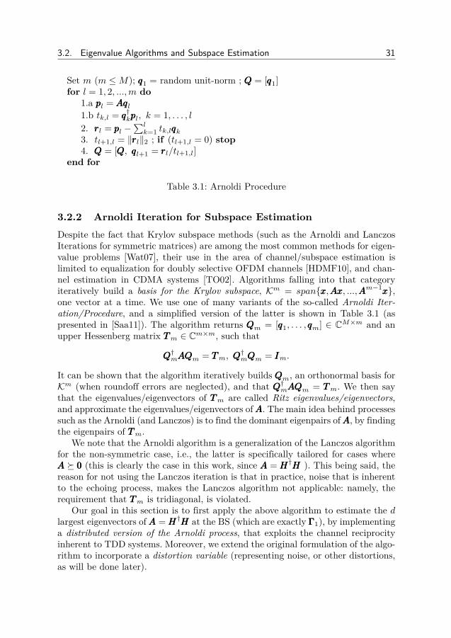
3.2.2 Arnoldi Iteration for Subspace EstimationDespite the fact that Krylov subspace methods (such as the Arnoldi and LanczosIterations for symmetric matrices) are among the most common methods for eigen-value problems [Wat07], their use in the area of channel/subspace estimation islimited to equalization for doubly selective OFDM channels [HDMF10], and chan-nel estimation in CDMA systems [TO02]. Algorithms falling into that categoryiteratively build a basis for the Krylov subspace, Km = spanxxx,AAAxxx, ...,AAAm−1xxx,one vector at a time. We use one of many variants of the so-called Arnoldi Iter-ation/Procedure, and a simplified version of the latter is shown in Table 3.1 (aspresented in [Saa11]). The algorithm returns QQQm = [qqq1, . . . , qqqm] ∈ CM×m and anupper Hessenberg matrix TTTm ∈ Cm×m, such that
QQQ†mAAAQQQm = TTTm, QQQ†mQQQm = IIIm.
It can be shown that the algorithm iteratively builds QQQm, an orthonormal basis forKm (when roundoff errors are neglected), and that QQQ†mAAAQQQm = TTTm. We then saythat the eigenvalues/eigenvectors of TTTm are called Ritz eigenvalues/eigenvectors,and approximate the eigenvalues/eigenvectors ofAAA. The main idea behind processessuch as the Arnoldi (and Lanczos) is to find the dominant eigenpairs ofAAA, by findingthe eigenpairs of TTTm.
We note that the Arnoldi algorithm is a generalization of the Lanczos algorithmfor the non-symmetric case, i.e., the latter is specifically tailored for cases whereAAA 000 (this is clearly the case in this work, since AAA = HHH†HHH ). This being said, thereason for not using the Lanczos iteration is that in practice, noise that is inherentto the echoing process, makes the Lanczos algorithm not applicable: namely, therequirement that TTTm is tridiagonal, is violated.
Our goal in this section is to first apply the above algorithm to estimate the dlargest eigenvectors ofAAA = HHH†HHH at the BS (which are exactly ΓΓΓ1), by implementinga distributed version of the Arnoldi process, that exploits the channel reciprocityinherent to TDD systems. Moreover, we extend the original formulation of the algo-rithm to incorporate a distortion variable (representing noise, or other distortions,as will be done later).

32 Subspace Estimation and Decomposition
It becomes clear at this stage, that the BS requires knowledge of the sequenceHHH†HHHqqqlml=1, needed for the matrix-vector product in step 1 (Table 3.1): the lattercan be accomplished by obtaining an estimate pppl, ofHHH
†HHHqqql, l ∈ m. Without anyexplicit CSI at neither the BS nor the MS, we exploit the reciprocity of the mediumto obtain such an estimate, via BS-initiated echoing: the BS sends qqql over the DLchannel, the MS echoes back the received signal in an A-F like fashion, over theuplink (UL) channel (following the process proposed in [WTW08], and detailed inSect. 3.2.1), i.e.,
DL : sssl = HHHqqql +www(r)l
UL : pppl = HHH†sssl +www(t)l = HHH†HHHqqql +HHH†www
(r)l +www
(t)l
= HHH†HHHqqql + wwwl (3.2.2)
where sssl is the received signal in the DL, www(t)l and www(r)
l are distortions at the BSand MS, respectively (representing noise for example).
After the echoing phase, the BS has an estimate, pppl, ofHHH†HHHqqql, as seen from (3.2.2).
The remainder of the algorithm follows the conventional Arnoldi Iteration, and isshown in the Subspace Estimation using Arnoldi (SE-ARN) procedure (Table 3.2).In addition to TTTm at the output of the algorithm, we define the matrices, TTTm, WWWm
and EEEm, as follows,
[TTTm]i,l =
qqq†iHHH
†HHHqqql, if l ≤ m, ∀i ≤ l‖rrrl‖2, if l < m, i = l + 10, otherwise
WWWm = [www1, ..., wwwm], EEEm = [QQQ†mWWWm]SL (3.2.3)
where rrrl is given in Step 2.b (Table 3.2). Note that similarly to the conventionalArnoldi Iteration, TTTm is an the upper Hessenberg matrix. It then follows from theabove definitions that
TTTm = TTTm + [QQQ†mWWWm]U . (3.2.4)
This can be easily verified by plugging in Step 1.b into 2.a in Table 3.2.At the output of the SE-ARN procedure, the dominant eigenpairs of HHH†HHH are
approximated by those of TTTm as follows. Let TTTm = ΘΘΘΛΛΛΘΘΘ−1 be eigenvalue decompo-sition of TTTm, where ΘΘΘ is the (possibly non-orthonormal) set of eigenvectors. Then,it can easily be shown that ΓΓΓ1 = qr(QQQm[ΘΘΘ]1:d) are the Ritz eigenvectors of HHH†HHH,where [ΘΘΘ]1:d has as columns the eigenvectors of TTTm associated with the d largesteigenvalues (in magnitude).
Remark 3.1. To be exact, the Ritz eigenvectors do not contain any estimationnoise. That being said, we stick to this nomenclature, with a slight abuse of def-inition. Moreover, ΣΣΣ1, the Ritz eigenvalues of HHH†HHH, come for free once the Ritzeigenvectors are obtained (Table 3.2).
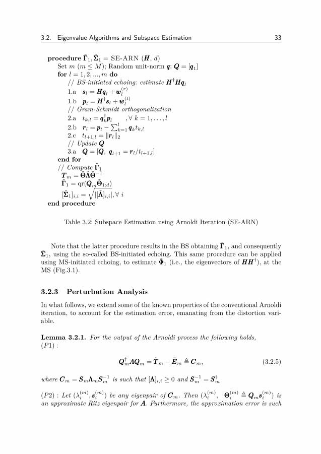
3.2. Eigenvalue Algorithms and Subspace Estimation 33
procedure ΓΓΓ1, ΣΣΣ1 = SE-ARN (HHH, d)Set m (m ≤M); Random unit-norm qqq; QQQ = [qqq1]for l = 1, 2, ...,m do
// BS-initiated echoing: estimate HHH†HHHqqql1.a sssl = HHHqqql +www
(r)l
1.b pppl = HHH†sssl +www(t)l
// Gram-Schmidt orthogonalization2.a tk,l = qqq†kpppl ,∀ k = 1, . . . , l2.b rrrl = pppl −
∑lk=1 qqqktk,l
2.c tl+1,l = ‖rrrl‖2// Update QQQ3.a QQQ = [QQQ, qqql+1 = rrrl/tl+1,l]
end for// Compute ΓΓΓ1TTTm = ΘΘΘΛΛΛΘΘΘ−1
ΓΓΓ1 = qr(QQQmΘΘΘ1:d)[ΣΣΣ1]i,i =
√|[ΛΛΛ]i,i|,∀ i
end procedure
Table 3.2: Subspace Estimation using Arnoldi Iteration (SE-ARN)
Note that the latter procedure results in the BS obtaining ΓΓΓ1, and consequentlyΣΣΣ1, using the so-called BS-initiated echoing. This same procedure can be appliedusing MS-initiated echoing, to estimate ΦΦΦ1 (i.e., the eigenvectors of HHHHHH†), at theMS (Fig.3.1).
3.2.3 Perturbation Analysis
In what follows, we extend some of the known properties of the conventional Arnoldiiteration, to account for the estimation error, emanating from the distortion vari-able.
Lemma 3.2.1. For the output of the Arnoldi process the following holds,(P1) :
QQQ†mAAAQQQm = TTTm − EEEm , CCCm, (3.2.5)
where CCCm = SSSmΛΛΛmSSS−1m is such that [ΛΛΛ]i,i ≥ 0 and SSS−1
m = SSS†m
(P2) : Let (λ(m)i , sss
(m)i ) be any eigenpair of CCCm. Then (λ(m)
i , ΘΘΘ(m)i , QQQmsss
(m)i ) is
an approximate Ritz eigenpair for AAA. Furthermore, the approximation error is such

34 Subspace Estimation and Decomposition
Figure 3.1: Proposed algorithm for Subspace Estimation using Arnoldi Iteration,and its resulting communication structure at BS and MS
that,
‖AAAΘΘΘ(m)i − λ(m)
i ΘΘΘ(m)i ‖22 ≤ c(i)m + ‖IIIM −QQQmQQQ
†m‖2F ‖WWWm‖2F , (3.2.6)
where c(i)m = ([TTTm]m+1,m|[sss(m)i ]m|)2.
(P3) : As m→M , ‖AAAΘΘΘ(m)i −λ(m)
i ΘΘΘ(m)i ‖22 → 0, implying that the eigenpairs of CCCm
perfectly approximate the eigenpairs of AAA(up to round-off errors).
Proof. The proof is shown in Appendix 3.6.1.
We underline the fact that if the distortion variable WWWm is zero, the above deriva-tions reduce to the well-known results on the Arnoldi process [Saa11, Sect. 6.2].Lemma 3.2.1 establishes the fact that each eigenpair (λ(m)
i , sss(m)i ) of CCCm, is asso-
ciated with one eigenpair (λ(m)i ,ΘΘΘ(m)
i ) of AAA.Though (P3) in Lemma 3.2.1 impliesthat the error in approximating the eigenpairs of AAA with those of CCCm vanishes asm → M , our simulations will later show that very good approximations can beobtained, even for mM .
Thus, one might be tempted to conclude at this point, that by computing theeigenpairs ofCCCm, one can perfectly estimate the eigenpairs ofAAA, despite the presenceof the distortion variable WWWm. However, the fact remains that CCCm , TTTm − EEEmcannot be computed, mainly because EEEm is not known to the BS. As a result, TTTm atthe output of the Arnoldi process will be used instead to approximate the eigenpairsof AAA. Now that we established that the eigenpairs of CCCm approximate that of AAA,the natural question is how close are the eigenpairs of TTTm, to that of CCCm.

3.3. Hybrid Analog-Digital Precoding for mmWaveMIMO systems 35
For that purpose, we first show the following,
CCCm +QQQ†mWWWm = (TTTm − EEEm) +QQQ†mWWWm
= TTTm + (QQQ†mWWWm − [QQQ†mWWWm]SL)= TTTm + [QQQ†mWWWm]U , TTTm (3.2.7)
where the first equality follows from the definition ofCCCm, and the last one from (3.2.4).Thus CCCm can be viewed as the matrix in question, and PPPm ,QQQ†mWWWm a perturba-tion matrix. We then apply the Bauer-Fike Theorem [GVL96, Th. 7.2.2] to boundthe difference in eigenvalues.
Lemma 3.2.2. Every eigenvalue λ of TTTm = CCCm +PPPm satisfies
|λ− λ| ≤√m ‖WWWm‖F ,
where λ is an eigenvalue of CCCm.
Proof. Refer to Appendix 3.6.2
Summarizing thus far, Lemma 3.2.1 showed that the eigenpairs of AAA can beapproximated by the eigenvalues of CCCm, with arbitrarily small error. However, sincethe latter is not available, we approximate the eigenpairs of CCCm (and consequentlyof AAA) by those of TTTm, the upper Hessenberg matrix at the output of the Arnoldiprocess. Finally, Lemma 3.2.2 established the fact that this approximation error, forthe eigenvalues, is upper bounded by the magnitude of the perturbation itself. Wenote that the relevant “error-metric” here is the distance between the true subspaceΓΓΓ1, and estimated subspace ΓΓΓ1 ∝ QQQmΘΘΘ1:d (Table 3.2). This does suggest that theestimation error is dependent on ΘΘΘ1:d, the eigenvectors of TTTm. However, performinga similar sensitivity analysis on the eigenvectors is much more involved, since thesensitivity of eigenvectors generally depends on the clustering of eigenvalues.
3.3 Hybrid Analog-Digital Precoding for mmWaveMIMOsystems
In this section we turn our attention to applying the above framework for subspaceestimation and precoding, to the hybrid analog-digital architecture. As this sectionwill gradually reveal, several obstacles have to be overcome for that matter. Westart by presenting some preliminaries that will be used throughout this section.
3.3.1 Preliminaries: Subspace DecompositionWe will limit our discussion to the digital and analog precoder, keeping in mindthat the same applies to the digital and analog combiner. In conventional MIMOsystems, the estimates of the right and left singular subspace, ΓΓΓ1 and ΦΦΦ1, obtained
36 Subspace Estimation and Decomposition
using SE-ARN, can directly be used to diagonalize the channel. However, the hybridanalog-digital architecture entails a cascade of analog and digital precoder. Thus,ΓΓΓ1 has to be decomposed into FFFGGG (hence the term Subspace Decomposition (SD)),as follows,
minFFF, GGG
h0(FFF ,GGG) = ‖ΓΓΓ1 −FFFGGG‖2Fs. t. h1(FFF ,GGG) = ‖FFFGGG‖2F ≤ d
FFF ∈ SM,d
(3.3.1)
We underline the fact that the authors in [EARAS+14] arrived to the same formu-lation as (3.3.1), and proposed a variation on the well-known Orthogonal MatchingPursuit (OMP), to tackle it. The same framework was recently extended in [MR-RGPH15] to relax the need for dictionaries based on the array response matrix. Analternate decomposition was proposed by [SY15b], where the optimization metric isthe user rate. Both works were published after the initial submission of our paper.
Within the context of hybrid precoding, the authors in [ZMK05] showed thatthere exists (non-unique) FFF ∈ SM,r, ggg ∈ Cr×1 such that ΓΓΓ1 = FFFggg, if and only ifr ≥ 2. This was extended in [MRRGPH15] where it was shown that there existsFFF ∈ SM,r,GGG ∈ Cr×d such that ΓΓΓ1 = FFFGGG, if r ≥ 2d. We note that for such cases,the cost function in (3.3.1) is zero, and we refer to such cases as optimal decompo-sition -whose performance we evaluate in the numerical results section: althoughthe aforementioned schemes use all the available RF chains for the decomposition(and our decomposition uses a subset of the RF chains), the sum-rate performanceis actually the same.
To a certain extent, (3.3.1) is reminiscent of formulations arising from areas suchas blind source separation, (sparse) dictionary learning, and vector quantization[XY13,AEB06]. Though there is a battery of algorithms and techniques that havebeen developed to tackle such problems, the additional hardware constraint on FFF ,i.e. FFF ∈ SM,r makes the use of such tools not possible. As a result, we will resort todeveloping our own algorithm. In spite of the non-convex and non-separable natureof the above quadratically-constrained quadratic program, we propose an iterativemethod that attempts to determine an approximate solution.
Block Coordinate Descent for Subspace Decomposition
In this part, we further assume that only d of the r available RF chains are used,i.e., FFF ∈ CM×d and GGG ∈ Cd×d (the reason for that will become clear later in thissection). The coupled nature of the objective and constraints in (3.3.1) suggestsa Block Coordinate Descent (BCD) approach. The main challenges arise from thecoupled nature of the variables in the constraint (since the latter makes convergenceclaims of BCD, not possible [RHL12]), and from the hardware constraint on FFF . Wewill show that a BCD approach implicitly enforces the power constraint in (3.3.1),and consequently the latter can be dropped without changing the problem.

3.3. Hybrid Analog-Digital Precoding for mmWaveMIMO systems 37
Our approach consists in relaxing the hardware constraint on FFF , and then ap-plying a Block Coordinate Descent (BCD) approach to alternately optimize FFF andGGG (while projecting each of the obtained solutions for FFF on SM,d). For that matter,we first define the Euclidean projection on the set SM,d in the following proposition.
Proposition 3.3.1. Let XXX ∈ CM×d be defined as [XXX]i,k = |xi,k| ejφi,k , ∀(i, k), and
YYY = ΠS [XXX] 4= argminUUU∈SM,d
‖UUU −XXX‖2F
denote its (unique) Euclidean projection on the set SM,d.Then [YYY ]i,k = (1/
√M) ejφi,k ,∀(i, k).
Proof. Refer to Appendix 3.6.4
The latter result implies that given an arbitrary FFF , finding the closest point toFFF , lying in SM,d simply reduces to setting the magnitude of each element in FFF , to1/√M .Neglecting the constraint on FFF in (3.3.1), one can indeed show that for fixed GGG
(resp. FFF ), the resulting subproblem is convex in FFF (resp. GGG). With this in mind,our aim is to produce a sequence of updates, FFF k,GGGkk such that the sequenceh0(FFF k,GGGk)k is non-increasing (keeping in mind that monotonicity cannot beshown due to the coupling in the power constraint). Thus, given GGGk, each of theupdates, FFF k+1 and GGGk+1, are defined as as follows,
(J1) FFF k+1 , minFFF
h0(FFF ) = ‖ΓΓΓ1 −FFFGGGk‖2F
(J2) GGGk+1 , minGGG
h0(GGG) = ‖ΓΓΓ1 −FFF k+1GGG‖2F
Both (J1) and (J2) are instances of a non-homogeneous (unconstrained) con-vex quadratically-constrained quadratic programming (QCQP) that can easily besolved (globally) by finding stationary points of their respective cost functions, toyield,
FFF k+1 = ΓΓΓ1GGG†k(GGGkGGG†k)−1 (3.3.2)
GGGk+1 = (FFF †k+1FFF k+1)−1FFF †k+1ΓΓΓ1 (3.3.3)
We note that our earlier assumption that only d of the RF chains are used here(i.e. GGG is square), guarantees that, (GGGlGGG†l ) in (3.3.3) is invertible, almost surely: infact, as our numerical results will later show, the incurred performance loss is quitenegligible.
Moreover, note that the solution in (3.3.2) does not necessarily satisfy the hard-ware constraint on FFF . Thus, the result of Proposition 3.3.1 can be used to compute

38 Subspace Estimation and Decomposition
procedure [FFF , GGG] = BCD-SD (ΓΓΓ1)Start with arbitrary FFF 0for k = 0, 1, 2, ... do
GGGk+1 ← (FFF †kFFF k)−1FFF †kΓΓΓ1FFF k+1 ← ΠS [ΓΓΓ1GGG
†k+1(GGGk+1GGG
†k+1)−1]
end forend procedure
Table 3.3: Block Coordinate Descent for Subspace Decomposition (BCD-SD)
the projection of FFF on SM,d. To prove our earlier observation that the optimal up-dates FFF k+1 and GGGk+1 satisfy the power constraint in (3.3.1), we plug (3.3.3) intothe following (dropping all subscripts for simplicity),
‖FFFGGG‖2F = tr
ΓΓΓ†1FFF (FFF †FFF )−1FFF †FFF︸ ︷︷ ︸=IIId
(FFF †FFF )−1FFF †ΓΓΓ1
≤ tr
((FFF †FFF )−1FFF †FFF
)tr(ΓΓΓ1ΓΓΓ†1
)= d (3.3.4)
where we assumed that ‖ΓΓΓ1‖2F = 1 w.l.o.g., and used the fact that tr(AAABBB) ≤tr(AAA)tr(BBB) for AAA,BBB 000. Note that the above relation holds for any arbitrary full-rank FFF , and thus, the power constraint is satisfied even after applying the projectionstep. The above shows that if BCD is used, then the power constraint in (3.3.1) isalways enforced. The corresponding method is termed Block Coordinate Descentfor Subspace Decomposition (BCD-SD), and is shown in Table 3.3.
Remark 3.2. We underline the fact that due to the projection step, one cannotshow that the sequence ho(FFF k,GGGk)k is non-increasing. Nevertheless, despite thefact that monotonic convergence of BCD-SD cannot be showed analytically, oursimulations indicate that the latter is indeed the case, under normal operatingconditions.
Remark 3.3. It can be easily verified that the optimal FFF ?,GGG? that maximize Rin (2.2.1) are such that ‖FFF ?GGG?‖ = d. Though the optimal solution to (3.3.1) is notinvariant to scaling, as far as the performance metric in (2.2.1) is concerned, therein no loss in optimality in scaling the solution given by BCD-SD, to fulfill the powerconstraint with equality.
One-dimensional case
Note that echoing (e.g., our proposed mechanism in Table 3.2) relies on the BSbeing able to send any vector qqql, to be echoed back by the MS. For the hybrid

3.3. Hybrid Analog-Digital Precoding for mmWaveMIMO systems 39
analog-digital architecture, this translates into the BS being able to (accurately)approximate qqql by fff lgl, where fff l is a vector, gl is a scalar. As a result, subspacedecomposition for the one-dimensional case is of great interest here. When d =1, (3.3.1) reduces to the problem below,
Lemma 3.3.1. Consider the single dimension SD problem,minfff, g
ho(fff, g) = ‖fff‖22 g2 − 2g<(fff†γγγ1)
s. t. [fff ]i = 1/√M ejφi ,∀i
(3.3.5)
where g ∈ R+ and [γγγ1]i = riejθi . Then the problem admits a globally optimum
solution given by, [fff?]i = 1/√M ejθi ,∀i and g? = ‖γγγ1‖1/
√M
Proof. Refer to Appendix 3.6.3
Similarly to (3.3.4), it can be verified that a power constraint is indeed implicitlyverified. Moreover, the approximation error eee , γγγ1 − fffg is such that,
[eee]i = |ri − ‖γγγ1‖1/M |ejθi , ∀i ∈ M. (3.3.6)
We note that when considering the effective beamformer, i.e., fffg, the solutiongiven by Lemma 3.3.1 is to some extent reminiscent of equal gain transmissionin [LH03,ZXLS07], in terms of the optimal phases.
We recall that a similar hybrid beamforming setup was considered in [ZMK05]where the authors optimize u,www,fff, g, to maximize the SNR as well as the spectralefficiency. Although our formulation optimizes the same quantities, the optimizationmetric we consider, the subspace distance, is different.
Column-wise Decomposition Note that the decomposition can be written ina simple form. Given a vector γγγ1, its globally optimal decomposition (from theperspective of (3.3.1)) is given as,
γγγ1 ≈ g?1fff?1 , (‖γγγ1‖1/
√M) ΠS [γγγ1].
This can be generalized to obtain an alternate method to BCD-SD, by decomposingΓΓΓ1, in a column-wise fashion,
ΓΓΓ1 = [γγγ1, · · · , γγγd] ≈ [g?1fff?1, · · · , g?dfff
?d]
, (1/√M) [ΠS [γγγ1], · · · ,ΠS [γγγd]] diag(‖γγγ1‖1, · · · , ‖γγγd‖1) (3.3.7)
Numerical Results
As mentioned earlier, (3.3.1) was formulated and solved in [EARAS+14], using avariation on the well-known Orthogonal Matching Pursuit (OMP), by recoveringFFF in a greedy manner, then updating the estimate of GGG in a least squares sense.
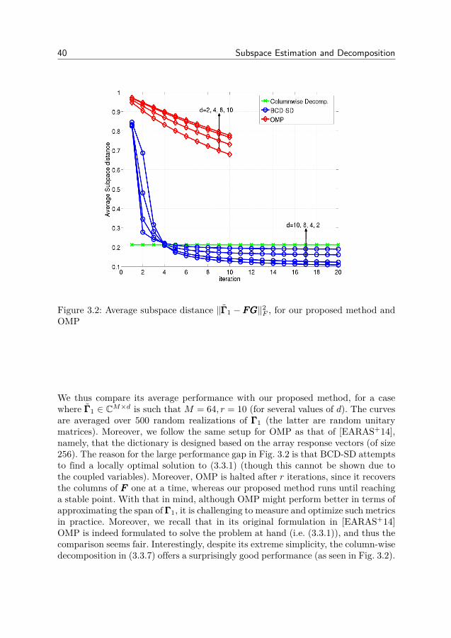
40 Subspace Estimation and Decomposition
Figure 3.2: Average subspace distance ‖ΓΓΓ1 −FFFGGG‖2F , for our proposed method andOMP
We thus compare its average performance with our proposed method, for a casewhere ΓΓΓ1 ∈ CM×d is such that M = 64, r = 10 (for several values of d). The curvesare averaged over 500 random realizations of ΓΓΓ1 (the latter are random unitarymatrices). Moreover, we follow the same setup for OMP as that of [EARAS+14],namely, that the dictionary is designed based on the array response vectors (of size256). The reason for the large performance gap in Fig. 3.2 is that BCD-SD attemptsto find a locally optimal solution to (3.3.1) (though this cannot be shown due tothe coupled variables). Moreover, OMP is halted after r iterations, since it recoversthe columns of FFF one at a time, whereas our proposed method runs until reachinga stable point. With that in mind, although OMP might perform better in terms ofapproximating the span of ΓΓΓ1, it is challenging to measure and optimize such metricsin practice. Moreover, we recall that in its original formulation in [EARAS+14]OMP is indeed formulated to solve the problem at hand (i.e. (3.3.1)), and thus thecomparison seems fair. Interestingly, despite its extreme simplicity, the column-wisedecomposition in (3.3.7) offers a surprisingly good performance (as seen in Fig. 3.2).
3.3. Hybrid Analog-Digital Precoding for mmWaveMIMO systems 41
3.3.2 Echoing in the Hybrid Analog-Digital ArchitectureIt is clear by now that the gist behind the schemes described in this work, is to ob-tain an estimate of HHH†HHHqqqlml=1 at the BS, by exploiting channel reciprocity, usingBS-initiated echoing described in (3.2.2). However, in the case of the hybrid analog-digital architecture, there are several issues that prevent the application of the latterprocedure. Firstly, the digital beamforming vector qqql needs to be approximated bya cascade of analog and digital beamformer, using the decomposition in Sect. 3.3.1,i.e., qqql = fff lgl + eeel, where eeel is the approximation error given in (3.3.6). More-over, the BS-initiated echoing relies on the MS being able to amplify-and-forwardits received signal: this is clearly not possible using the hybrid analog-digital ar-chitecture. In addition, neither the BS nor MS can digitally process the receivedsignal at the antennas: only after the application the analog precoder/combiner(and possibly the digital precoder/combiner) can the baseband signal be digitallymanipulated [WLP+09,EARAS+14].
With this in mind, we emulate the A-F step in BS-initiated echoing, (3.2.2),as follows. qqql is decomposed into fff lgl at the BS and sent over the DL. The MSlinearly processes the received signal in the downlink, with the analog combiner,i.e., sssl = WWW †l (HHHfff lgl), and same filter is used as the analog precoder, to processthe transmit signal in the UL, i.e., WWW lsssl. Finally, the received signal at the BS isprocessed with the analog precoder, FFF l. The resulting estimate, pppl, at the BS is,
pppl = FFF †lHHH†WWW lWWW
†lHHH(qqql − eeel) (3.3.8)
Note that the above process is possible using the hybrid analog-digital architecture.Since noise is present in any uplink/downlink transmission, for clarity in whatfollows, we drop the noise-related terms from all equations. Needless to say, theireffect is accounted for in the numerical results. It is clear from (3.3.8) that pppl is nolonger a “good” estimate of HHH†HHHqqql, for the reasons stated below.
1. Analog-Processing Impairments (API): Processing the signal at the MS withthe analog combiner/precoderWWW l greatly distorts the singular values/vectorsof the effective channel. Moreover, processing the received signal at the BSwith the analog combiner FFF l ∈ CM×r implies that pppl is now a low-dimensionalobservation of the desired M -dimensional quantity HHH†HHHqqql (since r < M).
2. Decomposition-Induced Distortions (DID): The error from decomposing qqqlat the BS, eeel, further distorts the estimate (as seen in (3.3.8)).
The above impairments are a byproduct of shifting the burden of digital precod-ing, to the analog domain. In what follows, these impairments will individually beinvestigated and addressed.
Cancellation of Analog-Processing Impairments
Our proposed method for mitigating analog-processing impairments (API) relies onthe simple idea of taking multiple measurements at both the BS and MS, and lin-
42 Subspace Estimation and Decomposition
early combining them, such thatWWW lWWW†l and FFF lFFF
†l approximate an identity matrix.
In the DL, qqql is approximated by fff lgl, and fff lgl is sent over the DL channel2,Kr times (where Kr = N/r), each linearly processed with an analog combinerWWW l,k ∈ CN×rKrk=1, to obtain the digital samples sssl,kKrk=1 (this process is shownin Table (3.4)). Moreover, the analog combiners are taken from the columns of aDiscrete Fourier Transform (DFT) matrix, i.e,
[WWW l,1, ...,WWW l,Kr ] = DDDr, (3.3.9)
where DDDr = 1√N
1 1 · · · 11 e−j
2πN · · · e−j
2(N−1)πN
......
...1 e−j
2(N−1)πN · · · e−j
2(N−1)2πN
. (3.3.10)
is a normalized N × N DFT matrix (i.e., where each column has unit norm andsatisfies the unit-modulus constraint). The same analog combiners, WWW l,kk, areused to linearly combine sssl,kk, to form sssl . We dub this procedure Repetition-Aided (RAID) Echoing, and the aforementioned DL phase, is shown in Table 3.4.The resulting signal at the MS, sssl, can be rewritten as,
sssl =(Kr∑k=1
WWW l,kWWW†l,k
)HHH(dfff lgl) = dHHHfff lgl, (3.3.11)
where equality follows from our earlier definition of WWW l,kk in (3.3.9). Note that theeffect of processing the received signal with the analog combiner has been completelysuppressed. Now, sssl is normalized, and echoed back in the UL direction.
A quite similar process is used in the UL: sssl is first decomposed into wwwlul, dRF chains are used to send it over the UL, Kt times (where Kt = M/r), and eachobservation is linearly processed with an analog combiner FFF l,m ∈ CM×rKtm=1.The resulting digital samples zzzl,mKtm=1 are again linearly combined with the sameFFF l,mm, to obtain the desired estimate pppl. Similar to the DL case, the analog com-biners are taken from the columns of a Discrete Fourier Transform (DFT) matrix,i.e, [FFF l,1, ...,FFF l,Kt ] = DDDt. The process for the UL is also shown in Table 3.4. Wecombine its steps to rewrite pppl as,
pppl =(
Kt∑m=1
FFF l,mFFF†l,m
)HHH†(dwwwlul) = dHHH†wwwlul (3.3.12)
2When sending fff lgl over the DL, we can use d RF chains, i.e.,
FFF lGGGl 111d = [fff l, · · · , fff l] diag(gl, · · · , gl) 111d = dfff lgl
thereby resulting in an array gain factor of d. Moreover, since we know from (3.3.4) that‖fff lgl‖2
2 ≤ 1, indeed this transmission scheme satisfies the power constraint. We also make use ofthis observation in the UL sounding.

3.3. Hybrid Analog-Digital Precoding for mmWaveMIMO systems 43
Figure 3.3: Repetition-aided (RAID) echoing for the hybrid analog-digital architec-ture
At the output of the RAID procedure, the BS has the following pppl,
pppl = dHHH†wwwlul = dHHH†(sssl − eee(r)l ) = dHHH†(dHHHfff lgl − eee
(r)l )
= d2HHH†HHHqqql − d2HHH†HHHeee(t)l − dHHH
†eee(r)l (3.3.13)
Note that eee(t)l = qqql − fff lgl (resp. eee(r)
l = sssl − wwwlul) is the error emanating fromapproximating qqql (resp. sssl) at the BS (resp. MS), that we dub BS-side (resp. MS-side) decomposition-induced distortion (DID). It is quite insightful to compare ppplin the latter equation with (3.3.8). We can clearly see that impairments originatingfrom processing the received signals with both WWW l and FFF l, have completely beensuppressed. In (3.3.13), pppl indeed is the desired estimate, i.e., HHH†HHHqqql, corruptedby distortions emanating from the BS-side decomposition, eee(t)
l , and the MS sidedecomposition, eee(r)
l (both investigated later in the next subsection). Both UL andDL phases of he process are illustrated in Fig. 3.3, and detailed in Table 3.4.
Remark 3.4. Note that employing this process reduces the hybrid analog-digitalarchitecture into a conventional MIMO channel: any transmitted vector in the DL,(fff lgl), can be received in a “MIMO-like” fashion, as seen from (3.3.11), at a costof Kr channel uses (the same holds for the UL, as seen from (3.3.12) ).
It can be seen from the above, that in the DL (resp. UL), d RF chains areactive at the BS (resp. MS), while all r RF chains are used at the MS (resp. BS),to minimize the overhead. With this in mind, it can be seen that the associated

44 Subspace Estimation and Decomposition
// DL phaseqqql = fff lgl + eee
(t)l
sssl,k = WWW †l,kHHH(dfff lgl), ∀k ∈ Krsssl =
∑Krk=1WWW l,ksssl,k
// UL phasesssl = wwwlul + eee
(r)l
zzzl,m = FFF †l,mHHH†(dwwwlul), ∀m ∈ Kt
pppl =∑Ktm=1FFF l,mzzzl,m
Table 3.4: Repetition-Aided (RAID) echoing
overhead with each echoing, Ω = (M +N)/r (channel uses), will decrease as moreRF chains are used.
Imperfect Compensation of Analog-Processing Impairments
Though the above method perfectly removes all artifacts of analog processing, theoverhead is proportional to (M+N)/r. A natural question is whether a similar resultcan still be achieved when DDDr and DDDt are truncated matrices i.e. when Kr < N/rand Kt < M/r. Perfect cancellation of API relies on a careful choice of the analogprecoder/combiner for each measurement, by picking WWW l,kKrk=1 and FFF l,mKtm=1 tospan all the columns of (square) DFT matrices. We investigate the effect of pickingDDDr and DDDt as truncated matrices, i.e. when Kr < N/r and Kt < M/r. Focusingour discussion on just analog precoders for brevity, we seek to find a (tall) matrixDDDt ∈ CM×(ηM), η < 1, such that,min
DDDt
‖ 1M IIIM − DDDtDDD
†t‖2F
s. t. DDDt ∈ SM, ηM .(3.3.14)
Due to the apparent difficulty of the problem, one can resort to stochastic optimiza-tion tools, e.g. simulated annealing: this approach is ideal for the design of DDDt (andDDDr as well), since it is completely independent of all parameters (except M,N andη), and can thus be computed off-line and stored for later use. Then, the resultingoverhead would be reduced to Ω = ηM+N
r .Let ΘΘΘl be the phase of DDDt at iteration l. Nc candidates for the phase update are
generated, by randomly perturbing each element in ΘΘΘl, i.e.
[BBBn]i,k = [ΘΘΘl]i,k + αl ui,k,∀(i, k), n = 1, ..., Nc,
where ui,k is a uniformly distributed random variable over [−π, π], and liml→∞
αl = 0.The candidate solution that yields the best value is selected. The algorithm shownin Table 3.5 can be used to find DDDt . Then, using exactly the same method, one

3.3. Hybrid Analog-Digital Precoding for mmWaveMIMO systems 45
Set α = 1, δ < 1, ΘΘΘ0 randomfor l = 0, 2, ..., I − 1 do
α = δαfor n = 1, ..., Nc do
[BBBn]i,k = [ΘΘΘl]i,k + α ui,k, ∀(i, k)CCCn = (1/
√M).ejBBBn
end forn? = argmax
n‖ 1M IIIM − CnC
†n‖2F
ΘΘΘl+1 = BBBn?
end forDDDt = (1/
√M).ejΘΘΘI
Table 3.5: Random Phase Search
can also design DDDr ∈ CN×(ηN) by formulating a similar problem as (3.3.14).Further investigations along this line are outside the scope of this work, but weopted to include them briefly, for completeness.
3.3.3 Proposed Algorithms
Combining the results of the previous subsections, we can now formulate our al-gorithm for Subspace Estimation and Decomposition (SED) for the hybrid analog-digital architecture (shown in Algorithm 1): estimates of the right / left singularsubspaces, ΓΓΓ1 and ΦΦΦ1, can be obtained by using the SE-ARN procedure (Sect. 3.2),keeping in mind that the echoing phase (Steps 1.a and 1.b) is now replaced by theRAID echoing procedure (Table 3.4. Then, the multi-dimensional subspace decom-position procedure, BCD-SD in Sect. 3.3.1, is then used to approximate each of theestimated singular spaces, by a cascade of analog and digital precoder/combiner.We highlight a desirable feature for the SED algorithm: the subspace estimationmechanism is totally decoupled from the subspace decomposition part, and thusany of the latter parts can be substituted, if desired.
Algorithm 1 Subspace Estimation and Decomposition (SED) for Hybrid Analog-Digital Architecture
// Estimate ΓΓΓ1 and ΦΦΦ1ΓΓΓ1, ΣΣΣ1 = SE-ARN (HHH, d)ΦΦΦ1 = SE-ARN (HHH†, d)// Decompose ΓΓΓ1 and ΦΦΦ1[FFF , GGG ] = BCD-SD (ΓΓΓ1, ρ)[WWW , UUU ] = BCD-SD (ΦΦΦ1, ρ)Perform waterfilling on ΣΣΣ1

46 Subspace Estimation and Decomposition
Note that previously proposed algorithms within this context such as the PMand TQR in [DCG04], are no longer applicable here: indeed both rely on the MSbeing able to amplify-and-forward its received signal at the antennas - clearly thismodus operandi cannot be supported by the hybrid analog-digital architecture.Interestingly, it is possible to apply elements from the RAID echoing structurethat we developed, effectively modifying the original echoing structure of the latterschemes, and adapting them to the hybrid analog-digital architecture (as shown inAlgorithm 2).
Algorithm 2 Modified Two-way QR (MTQR) for Hybrid Analog-Digital Archi-tecture
for l = 1, 2, ..., I do// Decompose each column of XXX
[XXX]n ≈ fffngn, ∀n ∈ d (using Lemma 3.3.1)XXX = [ fff1g1 , · · · , fffdgd ]
// Send XXX in DL, one column at a timeTTT k = WWW †kHHHXXX, ∀k ∈ KrYYY =
∑Krk=1WWW kTTT k ; YYY = qr(YYY )
// Decompose of YYY[YYY ]n ≈ wwwnun, ∀n ∈ d (using Lemma 3.3.1)YYY = [ www1u1 , · · · , wwwdud ]
// Send YYY in UL, one column at a timeSSSk = FFF †kHHH
†YYY , ∀k ∈ KtZZZ =
∑Ktk=1FFF kSSSk ; XXX = qr(ZZZ)
end for
Operationally, the proposed MTQR algorithm is the same as the Two-way QR(TQR) in [DCG04], whereby ΓΓΓ1 and ΦΦΦ1 are obtained iteratively: as I →∞,XXX → ΓΓΓ1(at BS) and YYY → ΦΦΦ1 (at MS). At each iteration of the algorithm, the BS sends XXXin the downlink, and the QR algorithm is applied to the received signal. Then, theresulting signal is sent by the MS in the uplink, and the QR algorithm is appliedat the BS to form YYY . While TQR assumes fully digital MIMO transmission, ourcontribution is to apply the RAID scheme, to make the transmission compatiblewith the hybrid analog-digital systems.
3.3.4 Bounds on Eigenvalue PerturbationIt can be clearly seen that the iterative nature of Algorithm 2 makes the applicationof Lemma 3.2.2, to quantify the impact of decomposition and approximation errors,not possible. On the other hand, for Algorithm 1, the fact that each HHH†HHHqqql is onlycorrupted by two sources of DID, eee(r)
l and eee(r)l , makes the latter possible. With
that in mind, we specialize the result of Sect. 3.2.2 and Lemma 3.2.2 (developedfor generic MIMO systems) to the case of Algorithm 1 in the hybrid analog-digital
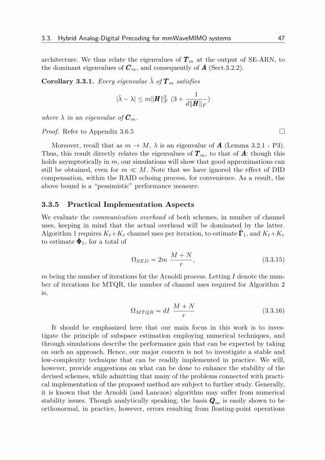
3.3. Hybrid Analog-Digital Precoding for mmWaveMIMO systems 47
architecture. We thus relate the eigenvalues of TTTm at the output of SE-ARN, tothe dominant eigenvalues of CCCm, and consequently of AAA (Sect.3.2.2).
Corollary 3.3.1. Every eigenvalue λ of TTTm satisfies
|λ− λ| ≤ m‖HHH‖2F (3 + 1d‖HHH‖F
)
where λ in an eigenvalue of CCCm.
Proof. Refer to Appendix 3.6.5
Moreover, recall that as m → M , λ is an eigenvalue of AAA (Lemma 3.2.1 - P3).Thus, this result directly relates the eigenvalues of TTTm, to that of AAA: though thisholds asymptotically in m, our simulations will show that good approximations canstill be obtained, even for m M . Note that we have ignored the effect of DIDcompensation, within the RAID echoing process, for convenience. As a result, theabove bound is a “pessimistic” performance measure.
3.3.5 Practical Implementation AspectsWe evaluate the communication overhead of both schemes, in number of channeluses, keeping in mind that the actual overhead will be dominated by the latter.Algorithm 1 requiresKt+Kr channel uses per iteration, to estimate ΓΓΓ1, andKt+Kr
to estimate ΦΦΦ1, for a total of
ΩSED = 2m M +N
r, (3.3.15)
m being the number of iterations for the Arnoldi process. Letting I denote the num-ber of iterations for MTQR, the number of channel uses required for Algorithm 2is,
ΩMTQR = dIM +N
r(3.3.16)
It should be emphasized here that our main focus in this work is to inves-tigate the principle of subspace estimation employing numerical techniques, andthrough simulations describe the performance gain that can be expected by takingon such an approach. Hence, our major concern is not to investigate a stable andlow-complexity technique that can be readily implemented in practice. We will,however, provide suggestions on what can be done to enhance the stability of thedevised schemes, while admitting that many of the problems connected with practi-cal implementation of the proposed method are subject to further study. Generally,it is known that the Arnoldi (and Lanczos) algorithm may suffer from numericalstability issues. Though analytically speaking, the basis QQQm is easily shown to beorthonormal, in practice, however, errors resulting from floating-point operations
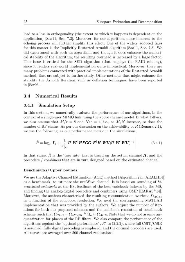
48 Subspace Estimation and Decomposition
lead to a loss in orthogonality (the extent to which it happens is dependent on theapplication) [Saa11, Sec. 7.3]. Moreover, for our algorithm, noise inherent to theechoing process will further amplify this effect. One of the widely adopted fixesfor this matter is the Implicitly Restarted Arnoldi algorithm [Saa11, Sec. 7.3]. Wedid experiment with such an algorithm, and though it does enhance the numeri-cal stability of the algorithm, the resulting overhead is increased by a large factor.This issue is critical for the SED algorithm (that employs the RAID echoing),since it renders real-world implementation quite impractical. Moreover, there aremany problems connected with practical implementations of the Restarted Arnoldimethod, that are subject to further study. Other methods that might enhance thestability the Arnoldi Iteration, such as deflation techniques, have been reportedin [Sor96].
3.4 Numerical Results
3.4.1 Simulation SetupIn this section, we numerically evaluate the performance of our algorithms, in thecontext of a single-user MIMO link, using the above channel model. In what follows,we also assume that M/r = 8 and N/r = 4, i.e., as M,N increase, so does thenumber of RF chains. As per our discussion on the achievability of R (Remark 2.1),we use the following, as our performance metric in the simulations,
R = log2
∣∣∣∣∣IIId + 1σ2
(r)UUU†WWW †HHHFFFGGGGGG†FFF †HHH†WWWUUU(UUU†WWW †WWWUUU)−1
∣∣∣∣∣ . (3.4.1)
In that sense, R is the ‘user rate’ that is based on the actual channel HHH, and theprecoders / combiners that are in turn designed based on the estimated channel.
Benchmarks/Upper bounds
We use the Adaptive Channel Estimation (ACE) method (Algorithm 2 in [AEALH14])as a benchmark, to estimate the mmWave channel. It is based on sounding of hi-erarchical codebooks at the BS, feedback of the best codebook indexes by the MS,and finding the analog/digital precoders and combiners using OMP [EARAS+14].Moreover, the authors characterized the resulting communication overhead ΩACE ,as a function of the codebook resolution. We used the corresponding MATLABimplementation that was provided by the authors. We adjust the number of iter-ations for both our proposed schemes and the codebook resolution of benchmarkscheme, such that ΩSED = ΩMTQR , Ωo ≈ ΩACE . Note that we do not assume anyquantization for phases of the RF filters. We also compare the performance of thealgorithms against the “optimal performance”, R? in (2.2.2), where full CSIT/CSIRis assumed, fully digital precoding is employed, and the optimal precoders are used.All curves are averaged over 500 channel realizations.

3.4. Numerical Results 49
Remark 3.5. Note that if one want to use “classical” pilot-based channel estima-tion to estimate the DL channel, i.e., a pilot sequence of minimum length M , thenthe same repetition-based framework that was used in RAID echoing, has to beused to cancel the effect of WWW from the effective channel estimate: it can be easilyseen that the resulting total (both DL and UL) number of pilots slots would be2MN/r2, thereby making the latter method infeasible.
3.4.2 Performance EvaluationWe start by investigating the performance of our schemes against the above bench-marks, for the case where M = 128, N = 64, L = 3, and m = 3d, for two cases:d = 1 and d = 2 where the resulting overhead is Ωo = 72 and Ωo = 144 chan-nel uses, respectively. It can be seen from Fig. 3.4 that both proposed schemesexhibit relatively similar performances, that are in turn very close to the optimalperformance bound R? (especially above −10 dB). This indeed suggests that themultiplexing gain achieved by conventional MIMO systems can still be maintainedin the hybrid analog-digital architecture, albeit at a much lower cost: the numberof required RF chains can be drastically decreased, resulting in savings in terms ofcost and power consumption. Moreover, we observe a sharp and significant perfor-mance gap between both our schemes and the benchmark from [AEALH14], overall SNR ranges (the gap being more significant in the low-SNR regime). We alsoevaluate the so-called optimal decomposition schemes [ZMK05,MRRGPH15] thatcan exactly decompose ΓΓΓ1 into FFFGGG (discussed in Sec. IV). Thus, the curves labeled’Optimal Decomp.’ refer to the case where the optimal decomposition is used in con-junction with SED. Fig 3.4 clearly reveals that the ability to optimally decomposethe estimated subspaces does not bring about additional gains. We note that thetiny mismatch between ’Optimal Decomp.’ and Algorithm 1 is due to simulationresolution.
We attempt to shed light on the stability of the proposed algorithms, as thenumber of paths in the mmWave channel, L, increases (where we set M = 64, N =32, d = 2,m = 6). For clarity we restrict the result to the low SNR regime. Thougha degradation in the performance of both algorithms is expected, as L increases,Fig. 3.5 clearly indicates that the latter degradation is not quite significant. Thoughnot visible here, our simulations show that this degradation is not present in themedium-to-high SNR region. As expected, this technique is best used for channelswith a few paths, e.g., mmWave channels.
We investigate the performance of both SED and MTQR in terms of averagesubspace angle, θ = E[α(ΓΓΓ1, ΓΓΓ1)] where α(ΓΓΓ1, ΓΓΓ1) (radians) is defined as the sub-space angle between ΓΓΓ1 and ΓΓΓ1 (implemented by computing the principal angles ofthe latter subspaces). As shown in Fig. 3.6, both schemes exhibit a similar behaviorof better estimation accuracy, as the SNR increases.
Remark 3.6. Though the performance of Algorithm 2 seems to be better, Fig. 3.4-3.6 both suggest that this gap is quite narrow. Moreover, both algorithms seem to

50 Subspace Estimation and Decomposition
−30 −25 −20 −15 −10 −5 0 5 100
5
10
15
20
25
30
SNR
Avera
ge u
ser
rate
R (
bps/H
z)
R*
Algorithm 1 (SED)
Algorithm 2 (MTQR)
Algorithm 2 [Alkhateeb] (ACE)
Optimal Decomp.
d=2, Ωo = 144
d=1, Ωo = 72
Figure 3.4: Average sum-rate of proposed schemes (M = 128, N = 64, d = 2, L =3,m = 6)
−30 −25 −20 −15 −10 −50
2
4
6
8
10
12
14
16
SNR
Avera
ge u
ser
rate
R (
bps/H
z)
R*
Algorithm 1 (SED)
Algorithm 2 (MTQR)
L=8
L=4
L=2
Figure 3.5: Effect of number of paths L, on the average user rate (M = 64, N =32, d = 2,m = 6)
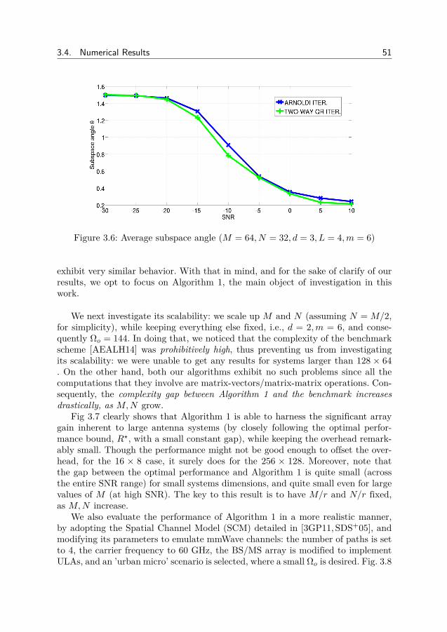
3.4. Numerical Results 51
Figure 3.6: Average subspace angle (M = 64, N = 32, d = 3, L = 4,m = 6)
exhibit very similar behavior. With that in mind, and for the sake of clarify of ourresults, we opt to focus on Algorithm 1, the main object of investigation in thiswork.
We next investigate its scalability: we scale up M and N (assuming N = M/2,for simplicity), while keeping everything else fixed, i.e., d = 2,m = 6, and conse-quently Ωo = 144. In doing that, we noticed that the complexity of the benchmarkscheme [AEALH14] was prohibitively high, thus preventing us from investigatingits scalability: we were unable to get any results for systems larger than 128 × 64. On the other hand, both our algorithms exhibit no such problems since all thecomputations that they involve are matrix-vectors/matrix-matrix operations. Con-sequently, the complexity gap between Algorithm 1 and the benchmark increasesdrastically, as M,N grow.
Fig 3.7 clearly shows that Algorithm 1 is able to harness the significant arraygain inherent to large antenna systems (by closely following the optimal perfor-mance bound, R?, with a small constant gap), while keeping the overhead remark-ably small. Though the performance might not be good enough to offset the over-head, for the 16 × 8 case, it surely does for the 256 × 128. Moreover, note thatthe gap between the optimal performance and Algorithm 1 is quite small (acrossthe entire SNR range) for small systems dimensions, and quite small even for largevalues of M (at high SNR). The key to this result is to have M/r and N/r fixed,as M,N increase.
We also evaluate the performance of Algorithm 1 in a more realistic manner,by adopting the Spatial Channel Model (SCM) detailed in [3GP11, SDS+05], andmodifying its parameters to emulate mmWave channels: the number of paths is setto 4, the carrier frequency to 60 GHz, the BS/MS array is modified to implementULAs, and an ’urban micro’ scenario is selected, where a small Ωo is desired. Fig. 3.8

52 Subspace Estimation and Decomposition
shows the average performance of such a system, with M = 64, N = 32,m = 2d,for several values of d (each resulting in different values for Ωo). Though both ouralgorithm and the benchmark exhibit similar performances for d = 1, this gapincreases with d, e.g. for d = 3 this performance gap is quite significant. Moreover,we can clearly see that Algorithm 1 yields a relatively high throughput in thisrealistic simulation setting (especially for d = 3), while still keeping the overheadat a relatively low level.
Evidently, increasing m (the number of iterations for the Arnoldi) has the effectenhancing the estimation accuracy (and increasing the communication overheadas well (3.3.15)). The marginal improvement brought about by increasing m, isdecreasing, and thus our simulations indicated that setting 2d ≤ m ≤ 3d providesa good trade-off.
3.4.3 Discussions
A few remarks are in order at this stage, regarding similarities and differences be-tween our two proposed algorithms. As discussed in Remark 3.6, when the commu-nication overhead is normalized, both SED and MTQR exhibit a similar behaviorand performance profile, across the entire SNR range (with a relatively small per-formance gap): indeed they can be used interchangeably with no change at all inthe operational requirements. However, as this work shows, we have an accurateanalytical description of the behavior of SED: the Arnoldi algorithm was adaptedto the subspace estimation part (with some analytical performance guarantees),and BCD-SD to mathematically describe the decomposition algorithm. In contrast,MTQR is a (heuristic) variation on the original TQR, whose behavior we have notmodeled analytically.
One of the conclusions suggested by all the above results, is the fact that the low-SNR performance of the proposed schemes is rather poor. However, interestingly,Figs. 3.4-3.8 unambiguously point out that this is the case for the benchmark schemeas well (ACE in [EARAS+14]): one might be tempted to conjecture at this pointthat this low-SNR behavior is an inherent aspect of mmWave channel estimation.Initial investigations reveal that, if more RF chains (more than r) can be employedduring the RAID echoing phase, the low-SNR performance can be greatly boosted.
3.5 Conclusion
We proposed an algorithm for blindly estimating the left and right singular subspaceof a mmWave MIMO channel, by exploiting channel reciprocity that is inherent toTDD systems. Though the algorithm is a perfect match for conventional (large)MIMO systems, we extended it to operate under the constraints dictated by thehybrid analog-digital architecture, and showed via simulations that it is a goodfit for large MIMO channels, with low rank, e.g., mmWave channels. Finally, oursimulations showed that a similar performance to the ideal case (fully digital perfect

3.5. Conclusion 53
−30 −25 −20 −15 −10 −5 0 5 100
5
10
15
20
25
30
35
SNR
Avera
ge u
ser
rate
R (
bps/H
z)
R*
Algorithm 1 (SED)
M=64 M=32
M=16
M=256
M=128
Figure 3.7: Average user-rate for different M,N (N = M/2, d = 2, L = 4,m =6,Ωo = 144)
−30 −25 −20 −15 −10 −5 0 5 100
5
10
15
20
25
30
35
40
SNR
Avera
ge u
ser
rate
R (
bps/H
z)
Algorithm 2 [Alkhateeb] (ACE)
Algorithm 1 (SED)
R*
d=3, Ωo=144
d=2, Ωo=96
d=1, Ωo=44
Figure 3.8: Average user-rate of proposed schemes over SCM channels (M = 64, N =32,m = 2d)

54 Subspace Estimation and Decomposition
CSI) can be achieved, with a only a few RF chains, thereby resulting in significantsaving in energy and cost, over conventional MIMO systems.
3.6 Appendix
3.6.1 Proof of Lemma 3.2.1(P1) : Combining steps (2.b) and (3.a) in the SE-ARN procedure, we write,
AAAqqql + wwwl =l+1∑i=1
[TTTm]i,l qqqi +l∑i=1
[EEEm]i,l qqqi , ∀l ∈ m,
We can rewrite the latter equation in matrix form, using the definitions of TTTm, WWWm
given in (3.2.3),
AAAQQQm + WWWm = QQQmTTTm + [TTTm]m+1,m qqqm+1bbb†m +QQQmEEEm (3.6.1)
where bbbm is the mth elementary vector, and EEEm = [QQQ†mWWWm]U . We can furthersimplify the above, using the fact that QQQ†mQQQm = IIIm and QQQ†mqqqm+1 = ooo,
QQQ†mAAAQQQm +QQQ†mWWWm = TTTm +EEEm
Using the definition of EEEm, we write,
QQQ†mAAAQQQm = TTTm + [QQQ†mWWWm]U −QQQ†mWWWm
= TTTm − EEEm , CCCm
where EEEm = [QQQ†mWWWm]SL, as defined in (3.2.3).
(P2) : Noting that TTTm +EEEm = CCCm +QQQ†mWWWm, we rewrite (3.6.1) as,
AAAQQQm −QQQmCCCm = [TTTm]m+1,m qqqm+1bbb†m − (IIIM −QQQmQQQ
†m)WWWm
Multiplying the latter equation by sss(m)i , and using the fact thatCCCmsss(m)
i = λ(m)i sss
(m)i ,
and QQQmsss(m)i = ΘΘΘ(m)
i
AAAΘΘΘ(m)i −λ(m)
i ΘΘΘ(m)i
= [TTTm]m+1,m qqqm+1bbb†msss
(m)i − (IIIM −QQQmQQQ
†m)WWWmsss
(m)i
Finally, the desired residual is upper bounded as,
‖AAAΘΘΘ(m)i − λ(m)
i ΘΘΘ(m)i ‖22
≤ ([TTTm]m+1,m|bbb†msss(m)i |)2 + ‖(IIIM −QQQmQQQ
†m)WWWmsss
(m)i ‖2F
≤ ([TTTm]m+1,m|[sss(m)i ]m|)2 + ‖IIIM −QQQmQQQ
†m‖2F ‖WWWm‖2F

3.6. Appendix 55
where the last inequality follows from ‖BBB1BBB2xxx‖22 ≤ ‖BBB1‖2F .‖BBB2‖2F .‖xxx‖22
(P3) : The proof immediately follows by noting that ‖IIIM −QQQmQQQ†m‖2F → 0 and
[TTTm]m+1,m → 0, as m→M , thereby implying that ‖AAAΘΘΘ(M)i − λ(M)
i ΘΘΘ(M)i ‖22 1.
3.6.2 Proof of Lemma 3.2.2
The proof follows from a direct application of the Bauer-Fike Theorem [GVL96,Th. 7.2.2]. Let CCCm = SSSmΛΛΛmSSS−1
m be the diagonalizable matrix in question, andTTTm = CCCm +PPPm the “perturbed” matrix. Then, every eigenvalue λ of TTTm satisfies,
|λ− λ|2 ≤ ‖SSSm‖22.‖SSS−1m ‖22.‖PPPm‖22 = ‖QQQ†mWWWm‖22
where λ is an eigenvalue of CCCm, and ‖BBB‖2 , σmax(BBB) is the vector-induced matrix2-norm. The last equality follows from the fact that SSSm is unitary, as discussed inLemma 3.2.1. Using the fact that ‖BBB‖2 ≤ ‖BBB‖F , we rewrite the last equation,
|λ− λ|2 ≤ ‖QQQ†mWWWm‖2F ≤ ‖QQQm‖2F ‖WWWm‖2F = m‖WWWm‖2F
This concludes the proof.
3.6.3 Proof of Lemma 3.3.1
Note that there is not loss in optimality by assuming the g ∈ R+. Moreover, exploit-ing the structure of ho, the globally optimal solution can be found by optimizingfor fff , assuming g is fixed (and vice) versa, i.e.,
fff?4=argmin
fffg2(fff†fff)− 2g<(fff†γγγ1), s. t. [fff ]i = 1/
√M ejφi
(a)⇔ φ?i =argmaxφi
1/√M <
(M∑i=1
ri ej(θi−φi)
)
φ?i =argmaxφi
M∑i=1<(ej(θi−φi)
)= θi
where (a) follows from applying the one-to-one mapping [fff ]i → 1/√M ejφi ,∀i.
Thus, [fff?]i = 1/√M ejθi ,∀i. Plugging fff? into the original problem, the optimiza-
tion of g is a simple unconstrained quadratic problem,
g?4= argmin
gg2 − 2g(‖γγγ1‖1/
√M) = ‖γγγ1‖1/
√M (3.6.2)

56 Subspace Estimation and Decomposition
3.6.4 Proof of Proposition 3.3.1Since YYY ∈ SM,d by definition (i.e., |[YYY ]i,k| = 1/
√M ) the problem just reduces to
finding the phase of each element in YYY . Thus,
YYY = ΠS [XXX] 4= argminUUU∈SM,d
‖UUU −XXX‖2F
(a)⇔ argminθi,k
∑i,k
|(1/√M)ejθi,k − xikejφi,k |2
⇔ θ?i,k = φ?i,k
where (a) follows from the fact that UUU i,k = (1/√M)ejθi,k ,∀UUU ∈ SM,d. Thus, we
conclude that [YYY ]i,k = (1/√M) ejφi,k ,∀(i, k). Furthermore, it follows from this
formulation that this projection is unique (despite the non-convexity of SM,d).
3.6.5 Proof of Corrollary 3.3.1The proof consists of finding a closed-from expression for WWWm as a function ofeee
(t)l and eee(r)
l , and applying the result of Lemma 3.2.2. Note that wwwl in (3.2.2) canrepresent any distortion, and by comparing pppl in both (3.2.2) and (3.3.13), can inferthat wwwl = −HHH†HHHeee(t)
l − (1/d)HHH†eee(r)l . Thus, WWWm in (3.2.3) can be written as,
WWWm = −HHH†HHH[eee(t)1 , · · · , eee(t)
m ]− (1/d)HHH†[eee(r)1 , · · · , eee(r)
m ]
, −HHH†HHHEEE(t) − (1/d)HHH†EEE(r)
Then using properties of the Frobenius norm,
‖WWWm‖F ≤ ‖HHH‖2F ‖EEE(t)‖F + (1/d)‖HHH‖F ‖EEE(r)‖F (3.6.3)
On the other hand, recall that eee(t)l = qqql− fff lgl and eee
(r)l = sssl− wwwlul. Thus, using the
results of Sec. 3.3.1,
‖eee(t)l ‖2 ≤ ‖qqql‖2 + ‖fff lgl‖2 ≤ 2
‖eee(r)l ‖2 ≤ ‖dHHHfff lgl‖2 + ‖wwwlul‖2 ≤ 1 + d‖HHH‖F
and it follows that
‖EEE(t)‖F ≤ 2√m, ‖EEE(r)‖F ≤
√m(1 + d‖HHH‖F ) (3.6.4)
The upper bound follows by combining (3.6.3) and (3.6.4).

Part II
Distributed Utility Optimization
57


Chapter 4
Preliminaries
4.1 Interference Management in Multiuser MIMONetworks
Going from single cell to multi-cell settings, interference has been widely recognizedas the limiting factor on the sum-rate performance. Many early works character-ized this using the analytical framework of degrees-of-freedom [CJ08]: the maxi-mum number of interference-free signaling dimensions in a given network. It wasalso shown that the maximum sum degrees-of-freedom (DoFs) of MIMO interfer-ence channels are a high SNR approximation of the capacity [CJ08] - the maximumperformance that can be achieved. Graphically, the sum DoFs corresponds to thehigh-SNR slope of the sum-rate vs SNR curve. With that in mind, it is also well-known that the presence of unsuppressed interference leads to a collapse in the DoFsof the network. The seminal works by M.A. Maddah-Ali, A.S. Motahari and A.K.Khandani on one hand, and V. Cadambe, K. Gomadam and S.A. Jafar indepen-dently, on the idea of Interference Alignment in wireless communication, highlightedthe intimate relation between IA and DoF maximization.
4.1.1 Coordination in Cellular NetworksThe ideas of coordinating signals from multiple BSs, in view of mitigating inter-ference, were considered much earlier, before the advent of CoMP. Such ideas wereearlier considered under the name of Virtual MIMO and Network MIMO. Theso-called Network MIMO concept was investigated in [KFVY06] and [ZCA+09],where full intra-cluster coordination (to enhance the sum-rate and limited inter-cluster coordination) was considered, for reducing interference for the cluster edgeusers. Though basic in nature, the idea of exploiting causally known interferencefor multi-cellular settings, dates as far back as [SZ01], where the “writing on dirtypaper” approach was employed to cancel interference that is known at the trans-mitter but not to the receiver. CoMP introduced the idea of cooperation among theBSs to mitigate inter-cell interference [GHH+10], and has been usually identified
59

60 Preliminaries
Figure 4.1: CoMP-CB (left) and CoMP-JT (right) (from [LSC+12] )
with several operation modes, Coordinated Beamforming (CB) and Joint Trans-mission (JT), being the most relevant ones here. Though they are both precodingtechniques, they are fundamentally different in their operation, and consequently,their inherent requirements and limitations [LSC+12].
CB is the setup where multiple BSs share their local CSI (i.e. channel informa-tion of each BS, to all the users), resulting in each BS having global CSI of all thechannels. Moreover, the data of each of the users is only available at its serving BS,and not shared among the other BSs. One instance of CB is to design the precodingvectors at each BS in such a way that interfering signals lie in the null space of eachuser’s desired signal subspace. This is illustrated in the left part of Fig 4.1 (whereinterfering transmissions are denoted in red): the precoding is done in such a waythat each BS’s transmission is orthogonal to all transmissions, by other BSs in thecoordination area. On the other hand, JT - in addition to sharing of CSI among theBSs (such that each BS has global CSI ), additionally requires the user data to beshared as well: each BS needs to know the data of all the users in the coordinationarea. The main idea behind JT is to design the precoding vectors at the BSs, insuch a way that each user is served by all the BSs (as illustrated in the right part ofFig 4.1). Stated differently, JT requires signals from each BS to align constructivelyat each MS. As a result, interference in the entire coordination region is turnedfrom destructive to constructive. Such ideas were initially put forth in [GHH+10].
Coordinated Beamforming
Coordination techniques that fall under the umbrella of CB are quite numerous anddiverse. Such techniques were the focus of many works, dating as far back as [GCJ11]

4.2. System Model 61
and [SSB+09]. In essence, schemes falling under this category iteratively refine theirrespective cost functions, in a fully distributed manner, i.e., only requiring local CSIat both users and BSs and alleviating the need for any backhaul between transmit-ters, or for any centralized compute node. Despite the massive number of CB-typeschemes falling under that category, they all employ the so-called framework offorward-backward training (detailed next, in Sect. 4.3.1).
Usually, such schemes can be categorized according to the metric that theyoptimize: such metrics mainly include (weighted) interference leakage [GCJ11],[GP11], (weighted) mean-squared error [SSB+09], [SRLH11], signal to interference-plus-noise ratio [GCJ11], [PH11], and (weighted) sum-rate [SGHP10a], [SRLH11][NSGS10] (an insightful and comprehensive comparison of such schemes was donein [SSB+13]). Despite the fact that the latter methods attempt to solve a problemthat is more generic than Interference Alignment (in a sense that they do not aim atsuppressing interference completely), in many of the above cases, there indeed existsan intimate relation between the two: for instance, in the high-SNR sum-rate max-imization problem, the precoder optimization problem reduces to finding transmitand receive filters, that satisfy the IA conditions (as formulated in [GCJ11]).
Interference Alignment
The concept of interference alignment in wireless communication was first presentedin [MAMK08], for the MIMO X channel. However, the concept was clearly crys-tallized in [CJ08], for the K-user Interference Channel (IC). The simple approachto solve the problem of interference in the interference channel is orthogonal accessin the time, frequency or spatial dimension (i.e. TDMA, FDMA, SDMA). As aresult, the resources of the channel (time, bandwidth, antennas, etc..) are dividedamong the users equally, i.e. each receiver gets 1/K from the total resources. How-ever with IA, every receiver can achieve 1/2 of the channel resources, regardlessof the number of users [CJ08]. This result is made possible by having every trans-mitter sacrifice half of its maximum signaling dimensions (time, frequency bands,antennas, etc...). Then, each transmitter-receiver pair can communicate over aninterference-free channel, regardless of the number of interferers [CJ09]. The capac-ity of any channel (the summation of the rates achieved by all the users) can beapproximated as follows [CJ08] : C ≈ d log(1 +SNR) where d is referred to as themultiplexing gain or the degrees-of-freedom (DoF) of the channel.
4.2 System Model
In this section we outline several of the canonical channel models that arise inthe context of multiuser communication and information theory (starting from themost generic one). We restrict our exposition to ones used throughout this part ofthe thesis.
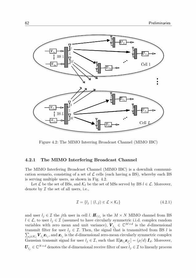
62 Preliminaries
UUU12
UUUL2
Figure 4.2: The MIMO Interring Broadcast Channel (MIMO IBC)
4.2.1 The MIMO Interfering Broadcast Channel
The MIMO Interfering Broadcast Channel (MIMO IBC) is a downlink communi-cation scenario, consisting of a set of L cells (each having a BS), whereby each BSis serving multiple users, as shown in Fig. 4.2.
Let L be the set of BSs, and Kl be the set of MSs served by BS l ∈ L. Moreover,denote by I the set of all users, i.e.,
I = lj | (l, j) ∈ L ×Kl (4.2.1)
and user lj ∈ I the jth user in cell l. HHH l,lj is the M ×N MIMO channel from BSl ∈ L, to user lj ∈ I (assumed to have circularly symmetric i.i.d. complex randomvariables with zero mean and unit variance), VVV lj ∈ CM×d is the d-dimensionaltransmit filter for user lj ∈ I. Then, the signal that is transmitted from BS l is∑j∈Kl VVV ljxxxlj , and xxxlj is the d-dimensional zero-mean circularly symmetric complex
Gaussian transmit signal for user lj ∈ I, such that E[xxxljxxxl†j] = (ρ/d) IIId. Moreover,
UUU lj ∈ CN×d denotes the d-dimensional receive filter of user lj ∈ I to linearly process
4.2. System Model 63
its received signal. The received signal, yyylj , for user lj ∈ I is,
yyylj = HHH l,ljVVV ljxxxlj +∑ik∈Iik 6=lj
HHHk,ljVVV ikxxxik +nnnlj , (4.2.2)
and the received signal of user lj ∈ I, after linear filtering, is given by,
xxxlj = UUU†
ljHHH l,ljVVV ljxxxlj +∑ik∈Iik 6=lj
UUU†
ljHHHk,ljVVV ikxxxik +UUU†
ljnnnlj , (4.2.3)
where the firs terms represents that desired signal, and the second one both intraand inter-cell interference. We further define the signal and interference covariancematrices of user lj ∈ I, as follows,
RRRlj = (ρ/d)HHH l,ljVVV ljVVV†
ljHHH†l,lj
and (4.2.4)
QQQlj =∑ik∈I
HHHk,ljVVV ikVVV†
ikHHH†k,lj −RRRlj , (4.2.5)
The MIMO IBC is the communication scenario that is investigated in Chap. 6.
Special Case: The MIMO Interference Channel The MIMO InterferenceChannel (MIMO IC) is known as the scenarios where a set L of transmit-receiveparts are sharing the same resource blocks (e.g. time, frequency). Each of the re-ceivers wishes to decode the signal originating from its own transmitter, subjectto interference from the remaining transmitters. In cellular networks, this wouldcorrespond to a set of L BSs, each serving a single MS, over the same resourceblock. Then, the MIMO IFC is a special case of the MIMO IBC.
4.2.2 The MIMO Interfering Multiple-Access ChannelThe MIMO Interfering Multiple-Access Channel (MIMO IMAC) represents an up-link communication scenario, in the context of cellular networks. In that sense, theMIMO IMAC is the “network dual” of the MIMO IBC. It comprises of a networkof L cells, each cell containing one BS, where BS l is serving a set Kl of MSs, andeach user wishes to send data to its serving BS (shown in Fig. 4.3).
We use the same notation as (4.2.1) to denote the total set of users, I,
I = lj | (l, j) ∈ L ×Kl (4.2.6)
where lj denotes the index of user j ∈ Kl, at BS l ∈ L. xxxik ∈ Cd represents the d-dimensional vector of independently encoded symbols sent by MS ik ∈ I (zero meancircularly symmetric), with covariance matrix E[xxxikxxx
†ik
] = (ρ/d)IIId. VVV ik ∈ CM×d

64 Preliminaries
Figure 4.3: The MIMO Interfering Multiple-Access Channel (MIMO IMAC)
denotes the d-dimensional transmit filter employed by transmitter ik ∈ I, HHH l,ik
the N ×M MIMO channel from MS ik ∈ I, to BS l, assumed to have circularlysymmetric i.i.d. complex random variables with zero mean and unit variance. Withthat in mind, the received signal at BS l ∈ L is given by,
yyyl =∑ik∈I
HHH l,ikVVV ikxxxik +nnnl, (4.2.7)
We denote by UUU lj ∈ CN×d the d-dimensional receive filter of user lj ∈ I. Afterlinear processing with the receive filter, the recovered signal vector of user j in celll, xxxlj , is given by,
xxxlj = UUU†
ljHHH l,ljVVV ljxxxlj +∑ik∈Iik 6=lj
UUU†
ljHHH l,ikVVV ikxxxik +UUU†
ljnnnl, ∀ lj ∈ I (4.2.8)
where the first term represents the desired signal, the second both intra and inter-cell interference, and nnnl represents the N -dimensional AWGN noise, such thatE[nnnlnnn†l ] = σ2IIIN . Moreover, RRRlj and QQQlj are the desired signal and interference

4.2. System Model 65
covariance matrices of user j’s signal, at BS l, respectively, and are given by,
RRRlj = (ρ/d) HHH l,ljVVV ljVVV†
ljHHH†l,lj
,
QQQlj = (ρ/d)∑ik∈I
HHH l,ikVVV ikVVV†
ikHHH†l,ik −RRRlj (4.2.9)
The MIMO IMAC is the communication scenario that is investigated in Chap. 5.
4.2.3 General RemarksNote that both the MIMO IBC and MIMO IMAC form the basis for deriving alldownlink and uplink models, i.e., every model is a special case of either one. Inthat sense, the MIMO Interference Channel and the MIMO Broadcast Channel(MIMO BC) are special cases of the MIMO IBC, and the MIMO Multiple-AccessChannel (MIMO MAC) is special case of the MIMO IMAC. Thus, we restrict ourpresentation in this chapter, to the MIMO IBC and MIMO IMAC.
Note that we use the term transmit filters / receiver filters in view of keepingnomenclature generic: this way, our framework is equally applicable to both MIMOIMAC and MIMO IBC. With that in mind, the transmit filters VVV lj represent theset of transmit precoders at the BSs (in the MIMO IBC context), and the transmitprecoders used by the UE’s (in the MIMO IMAC context). In addition, the receiverfilters UUU lj represent the set of receive filters at the UEs (in the MIMO IBCcontext), and the receive filter applied at the BSs (in the MIMO IMAC context).This is shown in Fig. 4.2 and Fig. 4.3
Note that in the above models (and what follows thereafter) we assume thatM,N and d are the same across users and BSs, for conciseness. However, this caneasily extended by adding the relevant indexes.
4.2.4 AssumptionsWe first make explicit the following definitions.
Definition 4.2.1 (Local and Global CSI). Given a network of transmitters / re-ceivers, global CSI refers to channel knowledge regarding all channels in the network.On the other hand, local CSI refers to the channels that are directly linked to atransmitter or receiver.
Definition 4.2.2 (Distributed Algorithm). In the scope of this thesis, an algorithmis classified as distributed if it requires local CSI at each transmitter and receiver.
We outline the main assumptions of this part in the thesis.
Assumption 4.2.1 (Local CSI). We assume that the users and BSs have localCSI, i.e., each user (resp. BS) knows the channels to its desired and interfering BSs(resp. users). We recall that investigating the CSI acquisition mechanism is not partof this work.
66 Preliminaries
Assumption 4.2.2 (Perfect CSI). CSI at each BS and user is assumed to beperfectly known, i.e., channel estimation errors are not accounted for.
Assumption 4.2.3 (Distributed Operation). All schemes are required to use localCSI only, using the framework of Forward-Backward training.
Assumption 4.2.4 (Decoding). Note that a common assumption in multi-useruplink communication scenarios, is that multi-user decoding is performed (e.g. suc-cessive interference cancellation). Due to the fact that such receivers are hard torealize in practice, we do not make such assumptions. Moreover, joint encoding anddecoding of each user’s desired streams in assumed, while interference is treated asnoise.
Assumption 4.2.5 (Low-Overhead Regime). Following the argument put forth inSect. 4.3.3, we restrict our proposed schemes to operate in the low-overhead regime,where only a small number of F-B iterations is used.
Assumption 4.2.6 (Transmit and receive power constraints). We underline thefact that most of the work thus far only enforces a power constraint on the pre-coder. The reason for that is the fact that communication in those setting is onlyone-directional, i.e. from transmitter to receiver, and thus no receive power con-straint is needed. However, our argument is as follows: when using distributedoptimization schemes employing F-B iterations, receivers are active in one of thephases (i.e., by sending pilots). Thus, generally, one does need a maximum transmitpower constraint for the receiver filter, in addition to the maximum transmit powerconstraint. In contrast to what has been done so far, we take this fact into accountin all our contributions, within this thesis: we impose a maximum power constraintfor both the transmitter and receiver.
4.3 Distributed CSI Acquisition
Obviously, all the methods discussed in the last section require each transmitterand receiver to have local CSI. In this part, the CSI acquisition mechanism isdistributed. Such a mechanism underlies all our proposed schemes in this part ofthe thesis, namely, the algorithms proposed in Chap. 5 and Chap. 6. And althoughthe investigation of different CSI acquisition mechanisms are outside the scope ofthe thesis, we briefly summarize that process, for completeness.
4.3.1 Forward Backward IterationsAlso known as ping-pong iterations, over-the-air iterations, and bi-directional train-ing. In the context of cellular networks, one of the fundamental building blocks fordistributed optimization techniques are the so-called Forward-Backward (F-B) it-erations. In brief, F-B iterations exploit the reciprocity of the network - which onlyholds in systems employing Time-Division Duplexing (TDD), and local CSI at each
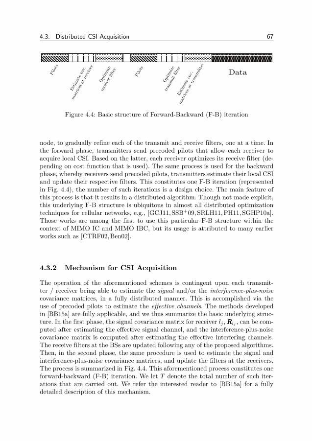
4.3. Distributed CSI Acquisition 67
DataEst
imat
eco
v.
mat
rice
sat
rece
iver
Pilo
ts
Opt
imize
rece
iver
filte
r
Opt
imize
tran
smit
filte
rEst
imat
eco
v.
mat
rice
sat
tran
smitte
r
Pilo
ts
Figure 4.4: Basic structure of Forward-Backward (F-B) iteration
node, to gradually refine each of the transmit and receive filters, one at a time. Inthe forward phase, transmitters send precoded pilots that allow each receiver toacquire local CSI. Based on the latter, each receiver optimizes its receive filter (de-pending on cost function that is used). The same process is used for the backwardphase, whereby receivers send precoded pilots, transmitters estimate their local CSIand update their respective filters. This constitutes one F-B iteration (representedin Fig. 4.4), the number of such iterations is a design choice. The main feature ofthis process is that it results in a distributed algorithm. Though not made explicit,this underlying F-B structure is ubiquitous in almost all distributed optimizationtechniques for cellular networks, e.g., [GCJ11,SSB+09, SRLH11,PH11,SGHP10a].Those works are among the first to use this particular F-B structure within thecontext of MIMO IC and MIMO IBC, but its usage is attributed to many earlierworks such as [CTRF02,Ben02].
4.3.2 Mechanism for CSI Acquisition
The operation of the aforementioned schemes is contingent upon each transmit-ter / receiver being able to estimate the signal and/or the interference-plus-noisecovariance matrices, in a fully distributed manner. This is accomplished via theuse of precoded pilots to estimate the effective channels. The methods developedin [BB15a] are fully applicable, and we thus summarize the basic underlying struc-ture. In the first phase, the signal covariance matrix for receiver lj ,RRRlj , can be com-puted after estimating the effective signal channel, and the interference-plus-noisecovariance matrix is computed after estimating the effective interfering channels.The receive filters at the BSs are updated following any of the proposed algorithms.Then, in the second phase, the same procedure is used to estimate the signal andinterference-plus-noise covariance matrices, and update the filters at the receivers.The process is summarized in Fig. 4.4. This aforementioned process constitutes oneforward-backward (F-B) iteration. We let T denote the total number of such iter-ations that are carried out. We refer the interested reader to [BB15a] for a fullydetailed description of this mechanism.

68 Preliminaries
4.3.3 Communication Overhead
Thus, for such schemes to be fully distributed (i.e. requiring only local CSI), therequired CSI quantities have to be obtained via uplink-downlink pilots and train-ing. As we can see, each F-B iteration has an associated communication over-heard, namely the cost of bi-directional transmission of pilots. Although many otherworks consider a more comprehensive definition of overhead (such as [EALH12]and [EALH11]), we adopt a more simplistic definition, keeping in mind that theactual overhead will be close to this quantity: it is the number of (minimal orthog-onal) pilots symbols needed for estimating the required CSI quantities (assumingthat minimal number of orthogonal pilots is used, i.e., d orthogonal pilot slots foreach uplink/downlink effective channel).
The complexity, pilot requirement, and number of forward-backward iterationsdepend on the type of global cost function that is being optimized. Simple costfunctions such as interference leakage [GCJ11] and MSE [SSB+09], were initiallyconsidered, and later extended to directly optimize more complex cost functionssuch as the sum-rate [SGHP10b], weighted sum-rate [SRLH11]. It becomes clearat this stage that the overhead associated with such schemes is largely dominatedby the number of such F-B iterations, before convergence is reached. That beingsaid, almost all schemes falling under the category of F-B iterations, require arelatively large number of such iterations, in the order of hundreds to thousands[SSB+13]. Moreover, this number seems to increase with the dimensions of thesystem. Consequently, this modus operandi is not feasible in a cellular network(since F-B iterations are carried out over-the-air, and the associated overhead wouldbe higher than the potential gains). We thus focus on a regime where T = 2 ∼ 5.
This major limitation became the object of recent investigations such as [KTJ13,BB15b,GKBS15,GKBS16b]. In our recent work, we also proposed algorithms withimproved convergence properties, using the interference leakage as cost function [GKBS15],and (lower bounds on) the sum-rate [GKBS16b] function. The proposed schemesachieve a similar performance as their conventional counterparts, however, with adrastically lower number of forward-backward iterations. Such schemes result inorders of magnitude reduction in overhead, over the conventional counterparts. Infact, one of the main contributions of this part (Chap. 6 and Chap. 5) is to designalgorithms that operate under a very low-overhead regime (where just a few F-Biterations are performed).
Although additional issues such as robustness and CSI error, have to consideredas well, such matter are outside the scope of our work (we refer the interested readerto [BB15a]).

4.4. Problem Formulation 69
4.4 Problem Formulation
4.4.1 Distributed Utility MaximizationWe refer to network-utility functions as a type of utility functions that are usedin the context of communication networks, namely, cellular networks in our work.With that in mind, distributed network-utility optimization refers to the processof designing distributed optimization algorithms, that optimize some network-widesum-utility function, over a set of optimization variables. In the context of cellularnetworks (more specifically, the MIMO IBC / MIMO IMAC), this can be writtenin generic from, as follows,
max uΣ =∑lj∈I ulj (UUU lj, VVV lj)
s. t. VVV lj ∈ Vlj , UUU lj ∈ Ulj , ∀ lj ∈ I(4.4.1)
where VVV lj ∈ CM×d and UUU lj ∈ CN×d are transmit and receive filter for user lj ∈ I,respectively. uΣ is the network-wide utility function (also called sum-utility func-tion), and ulj the utility of user lj ∈ I, defined as
ulj (UUU lj ,VVV lj) : CN×d × CM×dKL → R+ (4.4.2)
and assumed to be smooth and twice differentiable. Moreover, uΣ is assumed to be(additively) separable, i.e., uΣ =
∑lj∈I ulj (UUU lj , VVV lj)
Moreover, the sets Vlj and Ulj representing individual constraints (possibly non-convex), are assumed to be closed. While constraints arising in the context of thewireless communication can be quite diverse, in the proposed framework, they areassumed to be per-user, e.g., ‖VVV lj‖
2F ≤ Plj , ∀lj ∈ I and ‖UUU lj‖
2F ≤ Plj , ∀lj ∈ I.
The argument in favor of having a maximum transmit power constraint, for thereceiver as well, is discussed in Sect. 4.2.6 .
4.4.2 Block-Coordinate DescentThe framework under consideration entails tackling problems such as (4.4.1), usingthe well known Block-Coordinate Descent (BCD) method (described in Sect. 1.1.1):the block UUU lj is optimized, while the block VVV lj is assumed to be fixed (andvice-versa). Letting n denote the iteration index, the resulting method is formalizedbelow,
VVV n+1lj , argmax
VVV lj uΣ
UUUn+1lj , argmax
UUU lj uΣ(UUU lj, VVV
nlj)︸ ︷︷ ︸
J1
, VVV lj
︸ ︷︷ ︸
J2
, n = 1, 2, ...
(4.4.3)

70 Preliminaries
Moreover, the resulting subproblems are as follows,
(J1)
maxUUU lj
∑lj∈I ulj (UUU lj, VVV
nlj)
s. t. UUU lj ∈ Ulj ,∀lj ∈ I(4.4.4)
(J2)
maxVVV lj
∑lj∈I ulj (UUU
n+1lj, VVV lj)
s. t. VVV lj ∈ Vlj ,∀lj ∈ I(4.4.5)
Since uΣ is separable, then the latter problems can be rewritten in equivalent form,
(J1) : UUUn+1lj
argmaxUUU lj
ulj (UUU lj , VVVnlj)
s. t. UUU lj ∈ Ulj,∀lj ∈ I (4.4.6)
(J2) : VVV n+1lj
argmaxVVV lj
ulj (UUUn+1lj,VVV lj )
s. t. VVV lj ∈ Vlj ,∀lj ∈ I (4.4.7)
where UUUn+1lj
and VVV n+1lj
are local optimizers for (J1) and (J2), respectively , i.e.,UUUn+1lj
and VVV n+1lj
need not be globally optimal solutions to their respective problems,but only satisfy the KKT conditions.
Regarding convergence of the BCD method in(4.4.3) under the proposed frame-work, the latter can readily be established in a straightforward manner.
Proposition 4.4.1 (Monotonicity). Let ψn , uΣ(UUUnlj, VVVnlj), n = 1, 2, ... be the
sequence of iterates for the objective value. Then, ψn is non-decreasing in n, andconverges to a limit point, ψ0
The proof is simple. The application of each of the updates, UUUn+1lj and VVV n+1
lj,
cannot decrease the cost function,
uΣ(UUUnlj, VVVnlj) ≤ uΣ(UUUn+1
lj, VVV nlj) ≤ uΣ(UUUn+1
lj, VVV n+1
lj)
where the inequalities follow from the fact that the application of the optimalupdates for (J1) and (J2), UUUn+1
ljand VVV n+1
lj, cannot increase ψn. It follows that ψn
is non-decreasing, and there exists a limit point, ψ0, such that ψ0 = limn→∞ ψn
Thought monotonic convergence to a limit point is guaranteed, establishing thefact that the latter is a stationary point of uΣ obviously requires more conditions.If strong convexity for each of the subproblems, (J1) and (J2), can be established,the corresponding minimizers, UUUn+1
ljand VVV n+1
lj, are unique, and convergence to a
stationary point immediately follows.

4.4. Problem Formulation 71
As it will become clear, the above formulation encompasses a wide array ofnetwork-utility optimization problems. Thus it can be verified that a significantfraction of previous works is a special case of the latter, namely, mean-squared errorminimization [SSB+09, PH11], interference leakage minimization [GCJ11]. More-over, the two major contributions of this thesis, in this part, are alternate embod-iments of that framework: in Chap. 5, uΣ represents the so-called DLT bound (alower bound on the sum-rate), and in Chap. 6 uΣ represents the total interferenceleakage.
4.4.3 Sum-rate maximizationThe first utility in question is the sum-rate, defined as the sum of all individualachievable rates (across all users).
SRM for MIMO IBC
For the MIMO IBC setup in (4.2.1), the achievable rate of receiver lj is given by,
rlj = log2
∣∣∣∣IIId +(UUU†
ljRRRljUUU lj
)(UUU†
lj (QQQlj + σ2IIIN )UUU lj)−1
∣∣∣∣ , lj ∈ I (4.4.8)
Then, the corresponding sum-rate maximization problem (for the MIMO IBC) isformulated as follows,
(SRM − IBC)
max RΣ(UUU lj, VVV lj) =∑lj∈I rlj
s. t. ‖VVV lj‖2F ≤ Pt, ‖UUU lj‖
2F ≤ Pr ∀lj ∈ I
(4.4.9)
where Pt is the total power budget of transmitter lj , and Pr that power constraintof receiver lj (the argument for including a receive power constraint was discussedin Assumption 4.2.6). In contrast to previous formulations of (SRM − IBC) wherea sum-power constraint is used [SRLH11], we follow the main assumptions ofthe proposed framework (Sect. 4.4), and assume a per-user power constraint (asshown in the above problem) - keeping in mind that a sum-power constraint couldpotentially be handled. Note that the above problem degenerates into a the sum-rate maximization problem for MIMO IC, (SRM−IC), when one user is served byeach BS. And since the latter is NP-hard [RLL11], it follows that (SRM − IBC)is NP-hard as well.
Special Case: SRM for MIMO IC Following the signal model for the MIMOIC in (4.2.1), the achievable sum-rate of receiver l ∈ I is given by,
rl = log2
∣∣∣∣IIId +(UUU†
lRRRlUUU l
)(UUU†
l (QQQl + σ2IIIN )UUU l)−1
∣∣∣∣ , (4.4.10)
72 Preliminaries
We can then formulate the sum-rate maximization problem, (SRM−IC), as follows,
(SRM − IC)
max RΣ(UUU l, VVV l) =∑Ll∈I rl
s. t. ‖VVV l‖2F ≤ Pt, ‖UUU l‖2F ≤ Pr,∀ l ∈ I(4.4.11)
SRM for MIMO IMAC
Following the signal model for the MIMO IMAC setup in (4.2.2), the achievablerate of user lj ∈ I is given by,
rlj = log2 |IIId + (UUU†
ljRRRljUUU lj )(UUU†
lj (QQQlj + σ2IIIN )UUU lj )−1|, (4.4.12)
Then, the corresponding sum-rate maximization problem (for the MIMO IMAC isformulated as follows,
(SRM − IMAC)
max RΣ(UUU lj, VVV lj) =∑lj∈I rlj
s. t. ‖VVV lj‖2F ≤ Pt, ‖UUU lj‖
2F ≤ Pr, ∀lj ∈ I
(4.4.13)
The discussion motivating the use of a receive power constraint was discussed inAssumption 4.2.6. In contract the the MIMO IBC case, trying to impose the samesum-power constraint in the MIMO IMAC leads to a sum-power constraint acrossall UEs, in one cell: this is clearly not applicable in practice since it would hinderthe distributed nature of the algorithm. For the reasons above, a per-user constraintis the natural choice, in the sum-rate maximization problem for the MIMO IMAC,a per-user power allocation is assumed. Similarly to the MIMO IBC case, the NP-hardness of (SRM − IMAC) can be easily establish.
Relevant Work Despite the fact that most SRM problems are NP-hard, severalapproaches still tacked the latter problem. The authors in [SGHP10a] use BlockCoordinate Descent (BCD) to alternately optimize the transmit and receive fil-ter for a MIMO IC, while moving in the direction of sum-rate gradient at eachstep (convergence to a local minimum could not be shown due to the projectionstep). The weighted SRM problem for the MIMO IC was addressed in [NSGS10]where the authors exploit the equivalence between the weighted SRM problemand the Weighted MMSE problem to design an BCD-based algorithm to alter-nately optimize the transmit and receive filters (convergence to a local optimumwas shown). The same problem and algorithm was generalized in [SRLH11] forthe MIMO IBC setting, as the well known Weighted MMSE algorithm. Note thatthe above SRM problems (IBC, IC and IMAC) do not fall under the frameworkpresented in Sect. 4.4. However, the main contribution of Chap. 5 is to propose amechanism for circumventing the latter problem, by introducing a utility that wedub Difference of log and trace (DLT).

4.4. Problem Formulation 73
4.4.4 Interference Leakage Minimization
The interference leakage is yet another metric that is used for optimizing the per-formance of multiuser cellular networks. In contrast to (SRM) problems that arequite complicated, the leakage metric yields simple tractable expressions. Withinthe context of Interference Alignment for MIMO IC, the interference leakage min-imization (LM) problem was first formulated in [GCJ11]. We present it for thegeneric MIMO IBC case.
4.4.5 LM for MIMO IBC
Following the signal model introduced in Sect. 4.2.1, the Leakage Minimizationproblem (LM) is formulated as,
(LM − IBC)
min φ(UUU lj, VVV lj) =∑lj∈I tr(UUU
†
ljQQQljUUU lj )
s. t. UUU †ljUUU lj = IIId, VVV†
ljVVV lj = IIId, ∀lj ∈ I
(4.4.14)
It can be easily checked that (LM − IBC) belongs to the framework presentedin Sect. 4.4: φ is separable, and convex in each block of variables. Moreover, theresulting subproblem, has a unique solution (given by the eigenvectors of the co-variance matrix in question). The framework presented in Chap. 4.4 is fully ap-plicable. This is the basis of the well-known Distributed Interference Alignmentalgorithm [GCJ11].
Motivation It can be seen that (LM − IBC) is a “surrogate problem” for inter-ference alignment, in the sense that if φ = 0, then the IA conditions in Sect. 4.1.1are satisfied. Moreover, another motivation for leakage minimization problem is itsconnection to sum-rate maximization problem [GKBS15]. Referring to (4.4.9), asσ2 → 0 (high-SNR regime), the achievable rate rlj can be approximated by,
rlj = log2
∣∣∣UUU †ljRRRljUUU lj ∣∣∣− log2
∣∣∣UUU †ljQQQljUUU lj ∣∣∣Then, one can approximate (SRM − IBC) as follows,
(SRM − IBC) maxUUU
lj,VVV
lj
RΣ =K∑l=1
L∑j=1
rlj . (4.4.15)
By construction, algorithms based on interference leakage (referred to as subspacemethods) only optimize the interference subspace (as previously proposed algo-rithms in [GCJ11], [PH11]). Thus, by dropping the signal term in rlj , we can bound

74 Preliminaries
it as follows,
rlj ≥ − log2
∣∣∣UUU †ljQQQljUUU lj ∣∣∣ (a)≥
d∑i=1− log2
([UUU†
ljQQQljUUU lj ]ii)
(b)> −
d∑i=1
[UUU†
ljQQQljUUU lj ]ii = −tr(UUU†
ljQQQljUUU lj )
where (a) follows directly from applying Hadamard’s inequality, i.e. |AAA| ≤∏
[AAA]iifor AAA 000, and (b) from the fact that x > log2(x), ∀ x > 0. Although this resultis expected, it proves that minimizing the interference leakage at each user, resultsin optimizing a lower bound on the user’s high-SNR rate.
Related Work Several later works opted to use the interference leakage as met-ric for optimization due to its inherent simplicity (e.g., [PH11] and [GCJ11]). Theauthors in [MNM11] used the interference leakage as a metric, however, their for-mulation entails a constraint on the desired signal space. The main contribution ofthe thesis for the LM problem, is that of Chap. 6, where we investigate relaxingthe (LM − IBC) problem (replacing the unitary constraints with maximum powerconstraint), thereby speeding up the convergence of their proposed algorithm.Problem Statement: The goal for this part of the thesis is to develop algorithmsunder the umbrella of the above framework. Moreover, such algorithms should befast-converging (i.e., T = 2 ∼ 5 F-B iterations), with convergence that is shownanalytically.

Chapter 5
Sum-Rate MaximizationAlgorithms
We address the problem of sum-rate maximization in MIMO InterferingMultiple-Access Channels (MIMO IMAC) in this chapter. Due to theNP-hard nature of the problem (discussed in Chap. 4.2.2), we propose
to lower bound the problem using a so-called DLT bound (i.e., a difference of logand trace). We show that it is a lower bound on the sum-rate, shed light on itstightness, and underline a major advantage of using such a bound: The result-ing problem is an instance of the distributed network-utility optimization, and itthus leads to separable subproblems that decouple at both the transmitters andreceivers. Moreover, we derive the solution to the latter subproblem, that we dubnon-homogeneous waterfilling (a variation on the MIMO waterfilling solution), andunderline an inherent desirable feature: its ability to turn-off streams exhibitinglow-SINR, thereby greatly speeding up the convergence of the proposed algorithm.We then show the convergence of the resulting algorithm, max-DLT, to a stationarypoint of the DLT bound (a lower bound on the sum-rate).
We also propose a distributed algorithm dubbed Alternating Iterative MaximalSeparation (AIMS), that is a generalization of max-SINR [GCJ11]. Furthermore,we argue (and later verify via simulations) that this generalization offers superiorperformance over max-SINR. Finally, we rely on extensive simulation of various net-work configurations, to establish the superior performance of our proposed schemes,with respect to other state-of-the-art methods.
Remark 5.1. Though the paper addresses the problem at hand for a MIMO IMAC,it can be verified that the latter framework and methods are applicable to thenetwork-dual problem, the MIMO IBC, without modifications. Needless to say, italso applies to all ensuing special cases, such as the MIMO IFC, and the MIMOMultiple-Access Channel. This will be done in the numerical results section of thischapter.
Notation: In addition to the notation defined in Chap. 1, we define the following:for a given matrix AAA, AAA−† denotes (AAA†)−1.
75

76 Sum-Rate Maximization Algorithms
5.1 Maximizing DLT bounds
In this section we propose another approach to tackle the sum-rate optimizationproblem. The central idea behind this approach is to use a lower bound on the sum-rate, that results in separable sub-problems. Following the MIMO IMAC modelpresented in Chap. 4.2.2, the rate of user lj is given by,
rlj = log2 |IIId + (UUU†
ljRRRljUUU lj )(UUU†
ljQQQljUUU lj )−1|, (5.1.1)
where RRRlj and QQQlj are the desired signal and interference-plus-noise (IPN) covari-ance matrices for user j, at BS l, respectively, and are given by,
RRRlj = HHH l,ljVVV ljVVV†ljHHH†l,lj , lj ∈ I
QQQlj =L∑i=1
K∑k=1
HHH l,ikVVV ikVVV†ikHHH†l,ik + σ2
l IIIN −RRRlj , lj ∈ I.
and σ2l is the noise variance as BS l ∈ L. Moreover, we define,
RRRik = HHH†i,ikUUU ikUUU†ikHHHi,ik , ik ∈ I
QQQik =L∑l=1
K∑j=1
HHH†l,ikUUU ljUUU†ljHHH l,ik + σ2
ikIIIM − RRRik , ik ∈ I
as the signal and IPN covariance matrices of user ik, in the reverse network (whereσ2ik
is the noise variance at user ik). Finally, we henceforth denote LLLljLLL†lj
as theCholesky Decomposition of QQQlj , and KKKikKKK
†ik
as that of QQQikWe restate the resulting sum-rate maximization problem for the MIMO IMAC
(4.4.13), for convenience.
(SRM − IMAC)
max RΣ(UUU lj, VVV lj) =∑lj∈I rlj
s. t. ‖VVV lj‖2F = Pt, ‖UUU lj‖
2F = Pr, ∀lj ∈ I
(5.1.2)
Note that while the original formulation entails inequality constraints on the trans-mit/receive filters, we will adopt in this chapter, and equality (as seen above). Thereason for this choice will be discussed in details, in Chap 5.1.4. Our proposal isto lower bound rlj , using the so-called DLT bound, as follows,
r(LB)lj
, log2 |IIId +UUU†ljRRRljUUU lj | − tr(UUU†ljQQQljUUU lj ). (5.1.3)

5.1. Maximizing DLT bounds 77
5.1.1 Problem FormulationThe derivations leading up to r(LB)
ljare detailed in this section, focusing on interference-
limited case where the following holds,
λi[UUU†ljQQQljUUU lj ]→∞, ∀i ∈ d,
⇔
A1) λi[(UUU†ljQQQljUUU lj )
−1]→ 0, ∀i ∈ dA2) IIId (UUU†ljQQQljUUU lj )
−1 (5.1.4)
Proposition 5.1.1. When (UUU†ljQQQljUUU lj ) IIId, the user-rate rlj in (4.4.12) is lowerbounded by,
rlj ≥ log2 |IIId +UUU†ljRRRljUUU lj | − log2 |UUU†ljQQQljUUU lj |, (b.1)
≥ log2 |IIId +UUU†ljRRRljUUU lj | − tr(UUU†ljQQQljUUU lj ) , r(LB)lj
, (5.1.5)
where r(LB)lj
is such that,
∆lj , rlj − r(LB)lj
= tr(UUU†ljQQQljUUU lj )− log2 |UUU†ljQQQljUUU lj |
+O(tr[(UUU†ljQQQljUUU lj )(UUU†ljRRRljUUU lj )−1]), ∀lj ∈ I . (5.1.6)
Proof. Refer to Appendix 5.6.2.
The DLT bound, r(LB)lj
, shall be used as basis for the optimization algorithm.With that in mind, the sum-rate RΣ, can be lower bounded by R(LB)
Σ ,
R(LB)Σ
=∑lj∈I
log2 |IIId +UUU†ljRRRljUUU lj | − tr(UUU†ljQQQljUUU lj ) (5.1.7)
=∑ik∈I
log2 |IIId + VVV †ikRRRikVVV ik | − tr(VVV †ikQQQikVVV ik), (5.1.8)
where the last equality is due to log |III + AAABBB| = log |III + BBBAAA|, and the linearityof tr(.). Then, the MIMO IMAC sum-rate optimization problem in (5.1.2), can bebounded below by solving the following, max
VVV lj ,UUU lj R
(LB)Σ
s. t. ‖UUU lj‖2F = Pr, ‖VVV lj‖2F = Pt, ∀lj ∈ I(5.1.9)
Note that the above problem is not jointly convex in all the optimization variables,due to the coupling between the transmit and receive filters.
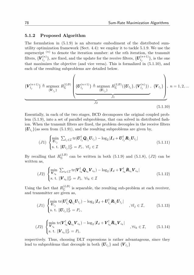
78 Sum-Rate Maximization Algorithms
5.1.2 Proposed AlgorithmThe formulation in (5.1.9) is an alternate embodiment of the distributed sum-utility optimization framework (Sect. 4.4): we employ it to tackle 5.1.9. We use thesuperscript (n) to denote the iteration number: at the nth iteration, the transmitfilters, VVV (n)
lj, are fixed, and the update for the receive filters, UUU (n+1)
lj, is the one
that maximizes the objective (and vice versa). This is formalized in (5.1.10), andeach of the resulting subproblems are detailed below.
VVV (n+1)lj
, argmaxVVV lj
R(LB)Σ
UUU (n+1)lj
, argmaxUUU lj
R(LB)Σ (UUU lj, VVV
(n)lj)︸ ︷︷ ︸
J1
, VVV lj
︸ ︷︷ ︸
J2
, n = 1, 2, ...
(5.1.10)
Essentially, in each of the two stages, BCD decomposes the original coupled prob-lem (5.1.9), into a set of parallel subproblems, that can solved in distributed fash-ion. When the transmit filters are fixed, the problem decouples in the receive filtersUUU lj(as seen from (5.1.9)), and the resulting subproblems are given by,
(J1)
minUUU lj
∑lj∈I tr(UUU
†ljQQQljUUU lj )− log2 |IIId +UUU†ljRRRljUUU lj |
s. t. ‖UUU lj‖2F = Pr, ∀lj ∈ I(5.1.11)
By recalling that R(LB)Σ can be written in both (5.1.9) and (5.1.8), (J2) can be
written as,
(J2)
minVVV ik
∑ik∈I tr(VVV
†ikQQQikVVV ik)− log2 |IIId + VVV †ikRRRikVVV ik |
s. t. ‖VVV ik‖2F = Pt, ∀ik ∈ I(5.1.12)
Using the fact that R(LB)Σ is separable, the resulting sub-problem at each receiver,
and transmitter are given as,
(J1)
minUUU lj
tr(UUU†ljQQQljUUU lj )− log2 |IIId +UUU†ljRRRljUUU lj |
s. t. ‖UUU lj‖2F = Pr,,∀lj ∈ I, (5.1.13)
(J2)
minVVV ik
tr(VVV †ikQQQikVVV ik)− log2 |IIId + VVV †ikRRRikVVV ik |
s. t. ‖VVV ik‖2F = Pt,,∀ik ∈ I, (5.1.14)
respectively. Thus, choosing DLT expressions is rather advantageous, since theylead to subproblems that decouple in both UUU lj and VVV lj
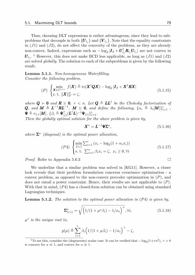
5.1. Maximizing DLT bounds 79
Thus, choosing DLT expressions is rather advantageous, since they lead to sub-problems that decouple in both UUU lj and VVV lj. Note that the equality constraintsin (J1) and (J2), do not affect the convexity of the problems, as they are alreadynon-convex. Indeed, expressions such as − log2 |IIId +UUU†ljRRRljUUU lj | are not convex inUUU lj . 1 However, this does not make BCD less applicable, as long as (J1) and (J2)are solved globally. The solution to each of the subproblems is given by the followingresult.
Lemma 5.1.1. Non-homogeneous Waterfilling.Consider the following problem,
(P )
minXXX∈Cn×r
f(XXX) , tr(XXX†QQQXXX)− log2 |IIId +XXX†RRRXXX|
s. t. ‖XXX‖2F = ζ.(5.1.15)
where QQQ 000 and RRR 000, r < n. Let QQQ , LLLLLL† be the Cholesky factorization ofQQQ, and MMM , LLL−1RRRLLL−†, MMM 000, and define the following, αi , λi[MMM ]ri=1 ,ΨΨΨ , v1:r[MMM ], βi , ΨΨΨ†(i)(LLL
†LLL)−1ΨΨΨ(i)ri=1.Then the globally optimal solution for the above problem is given by,
XXX? = LLL−†ΨΨΨΣΣΣ?, (5.1.16)
where ΣΣΣ? (diagonal) is the optimal power allocation,
(P4)
minxi
∑ri=1 (xi − log2(1 + αixi))
s. t.∑ri=1 βixi = ζ, xi ≥ 0,∀i
(5.1.17)
Proof. Refer to Appendix 5.6.3
We underline that a similar problem was solved in [KG11]. However, a closerlook reveals that their problem formulation concerns covariance optimization - aconvex problem, as opposed to the non-convex precoder optimization in (P ), anddoes not entail a power constraint. Hence, their results are not applicable to (P ).With that in mind, (P4) has a closed-form solution can be obtained using standardLagrangian techniques.
Lemma 5.1.2. The solution to the optimal power allocation in (P4) is given by,
ΣΣΣ?(i,i) =√(
1/(1 + µ?βi)− 1/αi)+,∀i, (5.1.18)
µ? is the unique root to,
g(µ) ,r∑i=1
βi
(1/(1 + µβi)− 1/αi
)+− ζ,
1To see this, consider the (degenerate) scalar case. It can be verified that − log2(1+ru2), r > 0is concave for u 1, and convex for u 1.
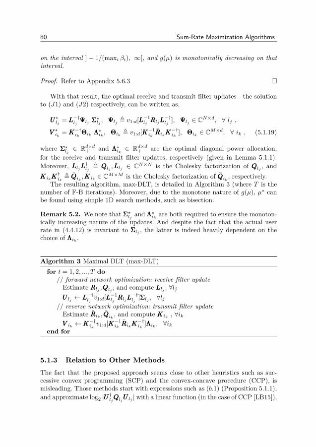
80 Sum-Rate Maximization Algorithms
on the interval ] − 1/(maxi βi), ∞[, and g(µ) is monotonically decreasing on thatinterval.
Proof. Refer to Appendix 5.6.3
With that result, the optimal receive and transmit filter updates - the solutionto (J1) and (J2) respectively, can be written as,
UUU?lj = LLL−†lj ΨΨΨlj ΣΣΣ?lj , ΨΨΨlj , v1:d[LLL−1ljRRRljLLL
−†lj
], ΨΨΨlj ∈ CN×d, ∀ lj ,
VVV ?ik = KKK−†ik ΘΘΘik ΛΛΛ?ik , ΘΘΘik , v1:d[KKK−1ikRRRikKKK
−†ik
], ΘΘΘik ∈ CM×d, ∀ ik , (5.1.19)
where ΣΣΣ?lj ∈ Rd×d+ and ΛΛΛ?ik ∈ Rd×d+ are the optimal diagonal power allocation,for the receive and transmit filter updates, respectively (given in Lemma 5.1.1).Moreover, LLLljLLL
†lj
, QQQlj ,LLLlj ∈ CN×N is the Cholesky factorization of QQQlj , andKKKikKKK
†ik
, QQQik ,KKKik ∈ CM×M is the Cholesky factorization of QQQik , respectively.The resulting algorithm, max-DLT, is detailed in Algorithm 3 (where T is the
number of F-B iterations). Moreover, due to the monotone nature of g(µ), µ? canbe found using simple 1D search methods, such as bisection.
Remark 5.2. We note that ΣΣΣ?lj and ΛΛΛ?ik are both required to ensure the monoton-ically increasing nature of the updates. And despite the fact that the actual userrate in (4.4.12) is invariant to ΣΣΣlj , the latter is indeed heavily dependent on thechoice of ΛΛΛik .
Algorithm 3 Maximal DLT (max-DLT)for t = 1, 2, ..., T do
// forward network optimization: receive filter updateEstimate RRRlj ,QQQlj , and compute LLLlj , ∀ljUUU lj ← LLL−†lj v1:d[LLL−1
ljRRRljLLL
−†lj
]ΣΣΣlj , ∀lj// reverse network optimization: transmit filter updateEstimate RRRik , QQQik , and compute KKKik , ∀ikVVV ik ←KKK−†ik v1:d[KKK−1
ikRRRikKKK
−†ik
]ΛΛΛik , ∀ikend for
5.1.3 Relation to Other MethodsThe fact that the proposed approach seems close to other heuristics such as suc-cessive convex programming (SCP) and the convex-concave procedure (CCP), ismisleading. Those methods start with expressions such as (b.1) (Proposition 5.1.1),and approximate log2 |UUU
†ljQQQljUUU lj | with a linear function (in the case of CCP [LB15]),
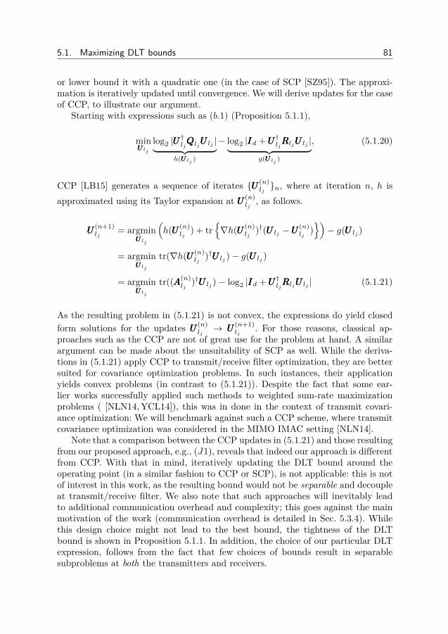
5.1. Maximizing DLT bounds 81
or lower bound it with a quadratic one (in the case of SCP [SZ95]). The approxi-mation is iteratively updated until convergence. We will derive updates for the caseof CCP, to illustrate our argument.
Starting with expressions such as (b.1) (Proposition 5.1.1),
minUUU lj
log2 |UUU†ljQQQljUUU lj |︸ ︷︷ ︸
h(UUU lj )
− log2 |IIId +UUU†ljRRRljUUU lj |︸ ︷︷ ︸g(UUU lj )
, (5.1.20)
CCP [LB15] generates a sequence of iterates UUU (n)ljn, where at iteration n, h is
approximated using its Taylor expansion at UUU (n)lj
, as follows.
UUU(n+1)lj
= argminUUU lj
(h(UUU (n)
lj) + tr
∇h(UUU (n)
lj)†(UUU lj −UUU
(n)lj
))− g(UUU lj )
= argminUUU lj
tr(∇h(UUU (n)lj
)†UUU lj )− g(UUU lj )
= argminUUU lj
tr((AAA(n)lj
)†UUU lj )− log2 |IIId +UUU†ljRRRljUUU lj | (5.1.21)
As the resulting problem in (5.1.21) is not convex, the expressions do yield closedform solutions for the updates UUU (n)
lj→ UUU
(n+1)lj
. For those reasons, classical ap-proaches such as the CCP are not of great use for the problem at hand. A similarargument can be made about the unsuitability of SCP as well. While the deriva-tions in (5.1.21) apply CCP to transmit/receive filter optimization, they are bettersuited for covariance optimization problems. In such instances, their applicationyields convex problems (in contrast to (5.1.21)). Despite the fact that some ear-lier works successfully applied such methods to weighted sum-rate maximizationproblems ( [NLN14,YCL14]), this was in done in the context of transmit covari-ance optimization: We will benchmark against such a CCP scheme, where transmitcovariance optimization was considered in the MIMO IMAC setting [NLN14].
Note that a comparison between the CCP updates in (5.1.21) and those resultingfrom our proposed approach, e.g., (J1), reveals that indeed our approach is differentfrom CCP. With that in mind, iteratively updating the DLT bound around theoperating point (in a similar fashion to CCP or SCP), is not applicable: this is notof interest in this work, as the resulting bound would not be separable and decoupleat transmit/receive filter. We also note that such approaches will inevitably leadto additional communication overhead and complexity; this goes against the mainmotivation of the work (communication overhead is detailed in Sec. 5.3.4). Whilethis design choice might not lead to the best bound, the tightness of the DLTbound is shown in Proposition 5.1.1. In addition, the choice of our particular DLTexpression, follows from the fact that few choices of bounds result in separablesubproblems at both the transmitters and receivers.

82 Sum-Rate Maximization Algorithms
5.1.4 Analysis and DiscussionsInterpretation We provide an intuitive interpretation of the problem in Lemma 5.1.1and its solution. It can be easily verified that αi , λi[LLL−1RRRLLL−†]ri=1 are also theeigenvalues of QQQ−1RRR (where RRR and QQQ represent the signal and IPN covariance ma-trix, respectively). Thus, αi acts as a (quasi)-SINR measure, for each of the datastreams. Moreover, it can be seen that the optimal power allocated to stream i,ΣΣΣ?(i,i) in (5.1.18), tends to zero as αi → 0, i.e., no power is allocated to streams thathave low-SINR.2 Moreover, note that βi represents the cost of allocating powerto each of the streams (this can be seen in (P4)). Thus, the non-homogeneous wa-terfilling solution in (5.1.16) simply allocates power to each of the streams, basedon the SINR and cost of each (possibly not allocating power to some streams).
Discussion We now discuss the reason for adopting the equality power con-straints for the problem at hand (i.e., (J1) and (J2)), by showing the limitationof using an inequality constraint. Note that in the noise-limited regime, σl 1, ∀l ∈ L, and consequently αi , λi[LLL−1RRRLLL−†] → 0, ∀i ∈ r. Using the factthat log(1 + y) ≈ y, y << 1, the optimal power allocation in (P4) is approximatedas,
r∑i=1
xi − log2(1 + αixi) ≈r∑i=1
xi − αixi =r∑i=1
(1− αi)xiαi→0≈
r∑i=1
xi (5.1.22)
When inequality constrains are considered, (P4) takes the following form,
min∑i
xi s. t.r∑i=1
βixi ≤ ζ, xi ≥ 0. (5.1.23)
One can see that the optimal solution is x?i = 0,∀i, and the optimal transmit/receivefilter in (J1) and (J2) is zero. Thus, operating with an inequality power constraintleads to degenerate solution, in the noise-limited regime. Though it might seem thatan equality power constraint makes (J1) and (J2) harder to solve, this is not thecase as both have non-convex cost functions already. Moreover, the convergence ofBCD is unaffected since the globally optimal solution is found for each subproblem(formalized in the next subsection).
Convergence of max-DLT Regarding convergence of the proposed algorithm,max-DLT, it is established using standard BCD convergence results.
Proposition 5.1.2. Let ψn , R(LB)Σ (UUU (n)
lj, VVV (n)
lj), n = 1, 2, ... be the sequence
of iterates for the objective value. Then, ψn is non-decreasing in n, and convergesto a stationary point of R(LB)
Σ (UUU lj, VVV lj)2Although the optimal power allocation to stream i is zero for some streams, i.e., ΣΣΣ(i,i) = 0,
in the actual implementation of the algorithm, ΣΣΣ(i,i) = δ where δ 1.

5.2. Generalizing max-SINR 83
Proof. The sequence ψn converges to a stationary point of the objective, since aunique minimizer is found at each step. This follows form BCD convergence resultsin [Tse01] and [LY73, Chap 7.8].
5.2 Generalizing max-SINR
In in part, we generalize the well-known max-SINR algorithm. This is not fullyaligned with this part of the thesis, as convergence of this algorithm cannot beshown (similarly to max-SINR). However, we included it for completeness, and dueto its superior performance over max-SINR.
5.2.1 Problem FormulationThe intuition is also to lower bound the (SRM − IMAC) in (5.1.2). We make useof the fact that log |XXX| is monotonically increasing on the positive-definite cone,i.e.,
log |XXX2| ≥ log |XXX1|, for XXX2 XXX1 000 (5.2.1)
Applying the above property, we lower bound rlj in (4.4.12) as,
rlj > log2 |(UUU†ljRRRljUUU lj )(UUU
†ljQQQljUUU lj )
−1|
= log2|UUU†ljRRRljUUU lj |
|UUU†ljQQQljUUU lj |, rlj , ∀lj ∈ I (5.2.2)
Note that rlj is an approximation of the actual user rate rlj , where the approxima-tion error is O(tr[(UUU†ljQQQljUUU lj )(UUU
†ljRRRljUUU lj )−1]) (refer to Appendix 5.6.2). Moreover,
bounds such as (5.2.2) are already prevalent in the MIMO literature. Thus, thesum-rate RΣ can be bounded below, as follows,
RΣ >∑lj∈I
rlj = log2(∏lj
qlj ), where qlj ,|UUU†ljRRRljUUU lj |
|UUU†ljQQQljUUU lj |
Since the log function is monotonic, the sum-rate maximization problem in (5.1.2)is lower bounded as,
(SRM)
maxUUU lj ,VVV lj
∏lj∈I qlj
s. t. ‖UUU lj‖2F = Pr , ‖VVV lj‖2F = Pt ,∀ lj ∈ I(5.2.3)
Referring to (SRM), qlj is the so-called Generalized Multi-dimensional RayleighQuotient (GMRQ. It is a well-know separability metric that is extensively in thestudy of linear discriminant analysis [Bis06, Chap. 4.1]. In a nutshell, it measurethe separation between the signal and IPN subspace. Consequently, given the signaland IPN covariance matrices, RRRlj and QQQlj , each receiver chooses its filter such tomaximize the separation between signal and IPN subspace.

84 Sum-Rate Maximization Algorithms
5.2.2 Maximization of Generalized Multi-dimensional RayleighQuotient
The main limitation of solving problems such (SRM) is the fact it is not jointlyconvex in all the optimization variables. Though Block Coordinate Decent (BCD)stands out as a strong candidate, one major obstacle persists: while the problemdecouples in the receive filters (as shown in (SRM)), attempting to write a similarexpression by factoring out the transmit filters, leads to a coupled problem. There-fore, we propose an alternative (purely heuristic) method: the receive filters areupdated as the solution to maximize the sum-rate (assuming fixed transmit filters),while the transmit filters are chosen as the solution of the reverse network sum ratemaximization (this same structure is implicitly exploited in max-SINR [GCJ11]),i.e.,
(SRMF )
maxUUU lj
∏lj∈I qlj (UUU lj ) =
|UUU†ljRRRljUUU lj |
|UUU†ljQQQljU
UU lj |
s. t. ‖UUU lj‖2F = Pr , ∀ lj ,(5.2.4)
(SRMB)
maxVVV ik
∏ik∈I pik(VVV ik) =
|VVV †ikRRRikVVV ik |
|VVV †ikQQQik
VVV ik |
s. t. ‖VVV ik‖2F = Pt , ∀ ik .(5.2.5)
In other words, assuming transmit filters as fixed, the receive filters are updatedsuch as to maximize the separability metric in the forward phase. Similarly, thetransmit filters are chosen to maximize the separability in the backward trainingphase. Moreover, as seen from the above problems, the objective in each subproblemis invariant to scaling of the optimal solution. Thus, they can be solved as uncon-strained problems, and optimal solutions can be scaled, without loss of optimality.
Before we proceed, we first require a solution to the GMRQ maximization. Thesolution to this problem was earlier proposed in [Pri03]. We provide a more genericsolution to the problem (Appendix 5.6.4).
Lemma 5.2.1. Consider the following maximization of the r-dimensional GMRQ,
XXX? , argmaxXXX∈Cn×r
q(XXX) = |XXX†RRRXXX||XXX†QQQXXX|
, (5.2.6)
where QQQ ∈ Sn×n++ , RRR ∈ Sn×n+ and r < n. The optimal solution to this non-convexproblem is given by
XXX? = LLL−†ΨΨΨVVV , (5.2.7)
where
LLLLLL† = QQQ, LLL ∈ Cn×n ,ΨΨΨ = v1:r[LLL−1RRRLLL−†], ΨΨΨ ∈ Cn×r ,
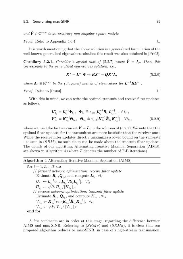
5.2. Generalizing max-SINR 85
and VVV ∈ Cr×r is an arbitrary non-singular square matrix.
Proof. Refer to Appendix 5.6.4
It is worth mentioning that the above solution is a generalized formulation of thewell-known generalized eigenvalues solution: this result was also obtained in [Pri03].
Corollary 5.2.1. Consider a special case of (5.2.7) where VVV = IIIr. Then, thiscorresponds to the generalized eigenvalues solution, i.e.,
XXX? = LLL−†ΨΨΨ⇔ RRRXXX? = QQQXXX?ΛΛΛr (5.2.8)
where ΛΛΛr ∈ Rr×r be the (diagonal) matrix of eigenvalues for LLL−1RRRLLL−†.
Proof. Refer to [Pri03].
With this in mind, we can write the optimal transmit and receive filter updates,as follows,
UUU?lj = LLL−†lj ΨΨΨlj , ΨΨΨlj , v1:d[LLL−1ljRRRljLLL
−†lj
] , ∀ lj ,
VVV ?ik = KKK−†ik ΘΘΘik , ΘΘΘik , v1:d[KKK−1ikRRRikKKK
−†ik
] , ∀ik , (5.2.9)
where we used the fact we can set VVV = IIId in the solution of (5.2.7). We note that theoptimal filter updates for the transmitter are more heuristic than the receiver ones:While the receive filter updates directly maximizes a lower bound on the sum-rate- as seen in (SRM), no such claim can be made about the transmit filter updates.The details of our algorithm, Alternating Iterative Maximal Separation (AIMS),are shown in Algorithm 4 (where T denotes the number of F-B iterations).
Algorithm 4 Alternating Iterative Maximal Separation (AIMS)for t = 1, 2, ..., T do
// forward network optimization: receive filter updateEstimate RRRlj ,QQQlj , and compute LLLlj , ∀ljUUU lj ← LLL−†lj v1:d[LLL−1
ljRRRljLLL
−†lj
], ∀ljUUU lj ←
√Pr UUU lj/‖UUU lj‖F
// reverse network optimization: transmit filter updateEstimate RRRik , QQQik , and compute KKKik , ∀ikVVV ik ←KKK−†ik v1:d[KKK−1
ikRRRikKKK
−†ik
], ∀ikVVV ik ←
√Pt VVV ik/‖VVV ik‖F
end for
A few comments are in order at this stage, regarding the difference betweenAIMS and max-SINR. Referring to (SRMF ) and (SRMB), it is clear that ourproposed algorithm reduces to max-SINR, in case of single-stream transmission,

86 Sum-Rate Maximization Algorithms
i.e., setting d = 1. Moreover, an inherent property of the max-SINR solution isthat it yields equal power allocation across all the streams (since the individualcolumns of each transmit/receive filter are normalized to unity). However, as evidentfrom (5.2.9), our proposed solution does not normalize the individual columns ofthe receive filter, but rather the whole filter norm (as seen in Algorithm 4). Thisallows for different power allocation, across columns of the same filter. That beingsaid, the proposed solution is expected to yield better sum-rate performance (w.r.t.max-SINR), especially in the interference-limited regime. This is due to the intuitivefact that much can be gained from allocating low power to streams that suffer fromsevere interference, and higher power to streams with lesser interference (this willbe validated in the numerical results section). We next introduce a rank adaptationmechanism that further enhances the interference suppression capabilities of thealgorithm.
5.2.3 AIMS with Rank AdaptationWe introduce one additional (heuristic) mechanism to robustify AIMS againstseverely interference-limited scenarios, by introducing a mechanism of Rank Adap-tation (RA): in addition to the transmit / receive filter optimization (Lemma 5.2.1),the latter allows the filter rank to be optimized as well. Mathematically speaking,RA addresses the following problem,
r? , argmaxr
[XXX? , argmax
XXX∈Cn×r
|XXX†RRRXXX||XXX†QQQXXX|
], (5.2.10)
Using the same argument as Lemma 5.2.1, one can verify that XXX? and r? are asfollows,
XXX? = [LLL−†ΨΨΨ]1:r? , where ΨΨΨ = v1:n[LLL−1RRRLLL−†]r? = argmax
r|ΛΛΛr| =
∣∣i | λi[LLL−1RRRLLL−† ≥ 1∣∣ (5.2.11)
where ΛΛΛr ∈ Rr×r is the (diagonal) matrix consisting of the r-largest eigenvalues ofLLL−1RRRLLL−†. Simply put, r? is the number of eigenvalues greater than one.
When RA is incorporated into AIMS, this mechanism will boost the performanceof the algorithm (namely in interference-limited settings). However, one still needsto ensure that the filter ranks for each transmit-receive pair are the same, i.e.,rank(UUU lj ) = rank(VVV lj ) ∀ lj . One quick (heuristic) solution is as follows. For eachtransmit-receive filter pair, compute the optimal filter rank for both the transmitand receive filter, and use the minimum.3 Needless to say, ensuring this conditionrequires additional signalling overhead. We thus envision RA, as potential “add-on” for AIMS, when one can afford the resulting overhead increase. In fact, rank-reduction offers a trade-off between reducing interference and diversity of the signal:
3 Alternately, one can apply RA to the receive filters only, in the last iteration of the algorithm,since the transmit filter updates are more heuristic than the receive filter updates.

5.3. Practical Aspects 87
however, in interference-limited scenarios, the former is more critical than the latter.This will be validated in the numerical results section.
5.3 Practical Aspects
5.3.1 ComparisonA few remarks are in order at this stage, regarding the similarities and differencesbetween AIMS and max-DLT. Referring to the optimal update equations for eachalgorithm, i.e., (5.2.9) and (5.1.19), we clearly see that both span the same subspace,i.e. the generalized eigenspace between the signal and IPN covariance matrices. Inaddition, max-DLT computes the optimal power allocation for each stream. Despitethis significant similarity among the two solutions, recall that they are derived fromtwo fundamentally different problems. While (5.2.9) is a heuristic (an extensionof max-SINR) that greedily maximizes the separability at each BS and user, theupdates in (5.1.19) maximize a lower bound on the sum-rate capacity (and areshown to converge to a stationary point of the DLT bound). That being said, theirperformance evaluation is done via numerical results.
5.3.2 BenchmarksAs mentioned earlier, we will also investigate the proposed approach in alternatescenarios such as MIMO IBC, and the MIMO Interference Channel (MIMO IFC).We benchmark our algorithms against widely adopted ones,
o max-SINR [GCJ11] in the MIMO IMAC, MIMO IFC and MIMO IBC
o MMSE and Weighted-MMSE [PH11,SRLH11] in the MIMO IFC and MIMOIBC
as well as relevant fast-converging algorithms,
o CCP-WMMSE [NLN14]: an accelerated version of WMMSE algorithm (usingCCP), for the MIMO IMAC
o IWU [GKBS15]: a fast-convergent leakage minimization algorithm for theMIMO IFC
Both IWU and CCP-WMMSE reply on the use of turbo iterations, where I inner-loop iterations are carried within each main F-B iteration. While those turbo itera-tions are carried at the BS/UE in the case of IWU, they are run over-the-air in thecase of CCP-WMMSE, thus leading to higher overhead. We note as well that earlierworks applied SCA to MIMO IBC settings, e.g., [KTJ12], but their algorithms arerestricted to beamforming/combining (no precoding).
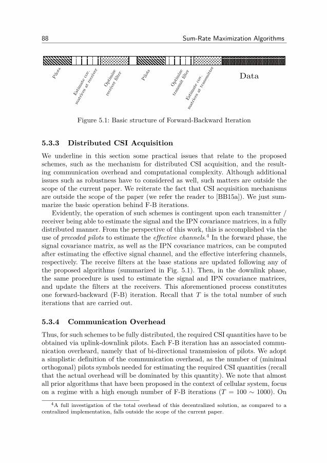
88 Sum-Rate Maximization Algorithms
DataEst
imat
eco
v.
mat
rice
sat
rece
iver
Pilo
ts
Opt
imize
rece
iver
filte
r
Opt
imize
tran
smit
filte
rEst
imat
eco
v.
mat
rice
sat
tran
smitte
r
Pilo
ts
Figure 5.1: Basic structure of Forward-Backward Iteration
5.3.3 Distributed CSI AcquisitionWe underline in this section some practical issues that relate to the proposedschemes, such as the mechanism for distributed CSI acquisition, and the result-ing communication overhead and computational complexity. Although additionalissues such as robustness have to considered as well, such matters are outside thescope of the current paper. We reiterate the fact that CSI acquisition mechanismsare outside the scope of the paper (we refer the reader to [BB15a]). We just sum-marize the basic operation behind F-B iterations.
Evidently, the operation of such schemes is contingent upon each transmitter /receiver being able to estimate the signal and the IPN covariance matrices, in a fullydistributed manner. From the perspective of this work, this is accomplished via theuse of precoded pilots to estimate the effective channels.4 In the forward phase, thesignal covariance matrix, as well as the IPN covariance matrices, can be computedafter estimating the effective signal channel, and the effective interfering channels,respectively. The receive filters at the base stations are updated following any ofthe proposed algorithms (summarized in Fig. 5.1). Then, in the downlink phase,the same procedure is used to estimate the signal and IPN covariance matrices,and update the filters at the receivers. This aforementioned process constitutesone forward-backward (F-B) iteration. Recall that T is the total number of suchiterations that are carried out.
5.3.4 Communication OverheadThus, for such schemes to be fully distributed, the required CSI quantities have to beobtained via uplink-downlink pilots. Each F-B iteration has an associated commu-nication overheard, namely that of bi-directional transmission of pilots. We adopta simplistic definition of the communication overhead, as the number of (minimalorthogonal) pilots symbols needed for estimating the required CSI quantities (recallthat the actual overhead will be dominated by this quantity). We note that almostall prior algorithms that have been proposed in the context of cellular system, focuson a regime with a high enough number of F-B iterations (T = 100 ∼ 1000). On
4A full investigation of the total overhead of this decentralized solution, as compared to acentralized implementation, falls outside the scope of the current paper.

5.3. Practical Aspects 89
the contrary, and in line with recent attempts such as [KTJ13,BB15b,GKBS15], weassume that this modus operandi is not feasible in the systems we consider (sinceF-B iterations are carried out over-the-air, and the associated overhead would behigher than the potential gains). We thus focus on a regime where T = 2 ∼ 5.In addition, we assume that the minimal number of orthogonal pilots is used, i.e.,d orthogonal pilot slots for each uplink/downlink effective channel. Moreover, thepilots are orthogonal across users and cells, resulting in a total of KLd orthogonalpilots for each uplink/downlink training phase. Consequently, the total overhead ofboth AIMS and max-DLT is approximately,
Ωprop = T (KLd︸ ︷︷ ︸UL
+KLd︸ ︷︷ ︸DL
) = 2TKLd channel uses.
It can be verified that the overhead is the same for benchmarks such as max-SINR, IWU and MMSE. Moreover, using similar arguments one can approximatethe overhead of CCP-WMMSE and WMMSE, as
Ωccp-wmmse = T [( KLM︸ ︷︷ ︸UL chann.estim
)×(L− 1)︸ ︷︷ ︸CSI
sharing
+ I︸︷︷︸turbo
×( KLN︸ ︷︷ ︸cov. matupd.
)] c. u.
Ωwwmse = T (KLd︸ ︷︷ ︸UL
+ KLM︸ ︷︷ ︸weights
+KLd︸ ︷︷ ︸DL
) c.u.
Though a coarse measure, we can see that the overhead associated with WMMSEand its fast-converging variant CCP-WMMSE are significantly higher than that ofthe proposed schemes. Moreover, CCP-WMMSE exhibits massively larger overheadthan the other two, namely due to the fact that the turbo optimization is carriedover-the-air (as described in Sec.5.3.2), and that the CSI for the uplink channels isshared among the BSs [NLN14]. The overhead of the aforementioned schemes willbe included in the numerical results.
5.3.5 ComplexityDespite the fact that the communication overhead is the limiting resource in cellularnetworks, we nonetheless shed light on the complexity of the proposed approaches,for completeness. By noticing that operations such as matrix multiplication andbisection search are quite negligible compared to other ones, both AIMS and max-DLT have similar computational complexity: it is dominated by the Cholesky De-composition of the IPN covariance matrix, and the Eigenvalue Decomposition ofMMM ,both of which have similar complexity of O(N3). Thus, the complexity is dominatedby,
Cprop = O(2KL(M3 +N3))
Note that the same holds for benchmarks such as max-SINR, IWU, and WMMSEsince they are dominated by matrix inversion of the IPN covariance matrix. While

90 Sum-Rate Maximization Algorithms
the complexity of CCP-WMMSE is also dominated by the above quantity, it alsoinvolves running a series of semi-definite programs (using interior point solvers),within each turbo iteration. This renders the algorithm quite costly.
5.4 Numerical Results
5.4.1 Simulation MethodologyWe use the achievable sum-rate in the network as the performance metric, wherethe achievable user rate is given by (4.4.12). Because the approach here is presentedin the context of MIMO IMAC, a significant fraction of the results will be underthe latter. As mentioned earlier, we will also investigate the proposed approachin alternate scenarios. We specialize our results to some MIMO IFC scenarios (aspecial case of the MIMO IMAC by setting K = 1), where interference alignmenthas been shown to be feasible [YGJK10]. We also investigate the MIMO IBC setup,since the proposed algorithms are equally applicable to that case, with little-to-nomodification.
As mentioned earlier, we also proposed another algorithm in this work, AIMS(a generalization of max SINR), whose development is not included here. We in-clude it in in this section for completeness. In this work, we assume a block-fadingchannel model with static users, where channel coefficients are drawn from inde-pendent and identically distributed complex Gaussian random variables, with zeromean and unit variance, for the sake of simplicity. We note at this point that weapplied our approaches to a much more realistic 5G setup. Since a description of theresulting simulation methodology is rather lengthly, we refer the interested readersto [MET15][Sect. 3.3.3]. In addition, we limit the number of F-B iterations, T , to asmall number. We further assume that both the signal and IPN covariance matricesare perfectly estimated at the transmitter / receiver, i.e., we do not model channelestimation errors. Finally, we note that all curves are averaged over 500 channelrealizations.
5.4.2 Results for Standard ScenariosWe first investigate the performance of such schemes in conventional canonicalscenarios, for benchmarking. We distinguish among feasible, proper and impropersetups [YGJK10].
MIMO IFC We start with a feasible MIMO IFC scenario, by setting M = N =4, d = 2 and fixing the number of F-B iterations, T = 4, for all schemes. We evalu-ate the sum-rate of both our algorithms against other well-known algorithms suchmax-SINR [GCJ11], MMSE [PH11], the rank-reducing algorithm (IWU-RR) earlierproposed in [GKBS15] (since such algorithms are designed for scenarios where fastconvergence is desired). We also included Weighted-MMSE with the correspondingnumber of F-B iterations (T = 4), and a large enough number of iterations (as an

5.4. Numerical Results 91
upper bound). It is clear from Fig. 5.2 that while max-DLT has similar performanceas W-MMSE (for T = 4) in the low-to-medium SNR regime, the gap increases in thehigh-SNR region (SNR ≥ 20 dB). Moreover, we note that our proposed schemes,outperform all other benchmarks, across all SNR regimes. In particular, the per-formance gap between max-DLT and the benchmarks, is quite significant in themedium-to-high SNR region. Moreover, despite the fact that only the rank-reducingscheme and max-DLT are able to achieve some degrees-of-freedom gain, max-DLToffers a 35% gain over the rank reducing scheme. Though max-DLT and IWU-RRare able to turn off some streams in view of reducing interference, the significantperformance gap is due to the fact that max-DLT also optimizes the signal subspaceas well. Finally, we note that the high-SNR performance of max-DLT is indicative ofthe fact it is able to achieve some to degrees-of-freedom, while the others algorithmsseem to have a significant amount of residual interference, i.e., no degrees-of-freedomgain. Note that the ‘optimal-performance’ of WMMSE is achieved for T = 200, butthe resulting overhead is massive. Although the performance of max-DLT is similarto WMMSE (T = 4) in low-to-medium SNR regime, the overhead is much lowerfor the former. Moreover, the gap increases in the medium-to-high SNR region.
MIMO IMAC We next evaluate MIMO IMAC setting with L = 2,K = 2,M =4, N = 4, d = 2, as a function of the number of F-B iterations, T . We also bench-mark against CCP-WMMSE (summarized in Sec. 5.3.2) by varying the numberof turbo iterations I, and testing the resulting performance and overhead. Fig. 5.3clearly shows the fast-converging features of both algorithms. More specifically, thisis apparent in the case of max-DLT, that reaches 95% of its performance in 2 itera-tions. While the performance of max-DLT is slightly better than CCP-WWMMSEfor I = 1, the overhead of the latter is twice that of the former (CCP-WMMSEbecomes better than max-DLT for I = 2, but the resulting overhead is thrice ashigh). Note that the ‘full’ performance CCP-WMMSE is achieved for I = 50, butthe the resulting overhead (and complexity) are orders-of-magnitude larger than theproposed schemes. Its performance is quite sensitive to solving the inner problemto optimality (i.e., until the turbo iteration converges), thus making it ill-suited forlarger setups. Indeed, the running time of CCP-WMMSE (using a mosek solver inCVX) prevented us form testing its performance for larger antenna configurations.
Proper MIMO IBC As mentioned earlier, our schemes are equally applicable toMIMO IBCs. For that matter, we investigate their performance in a proper MIMOIBC setup with 8 × 2 (single-stream) MIMO links, with L = 3,K = 3 (for severalSNR values). We benchmark our results against the well-known Weighed-MMSE(WMMSE) algorithm [SRLH11]. Note that for the latter, we keep the sum-powerconstraint that is employed by WMMSE, and adjust the per-user transmit powerconstraint Pt, for our algorithms, assuming equal power allocation among users.5
5If ρ is the per-BS sum-power constraint for WWMMSE, then ρ/K is the per-user transmitpower constraint for our algorithms.

92 Sum-Rate Maximization Algorithms
1/ σ2 (dB)
0 10 20 30 40
Su
m-r
ate
(b
ps/H
z)
0
10
20
30
40
50
60Sum-rate for M = 4, N = 4, L = 3, K = 1, d = 2, it = 4
max-DLTAIMSMMSE [Peters]max-SINRIWU - RRWMMSE (T=200)WMMSE (T=4)
Figure 5.2: Ergodic sum-rate for L = 3,K = 1,M = N = 4, d = 2, T = 4 (feasibleMIMO IFC)
1 2 3 4 5 6 7 810
15
20
25
30
35
40
T
Sum
−ra
te (
bps/H
z)
Sum−rate for M = 4, N = 4, L = 2, K = 2, d = 2, it = 8, SNR=20
max−DLT (Ω=16T)
AIMS (Ω=16T)
max−SINR (Ω=16T)
CCP−WMMSE
I = 1, Ω=32T
I = 2, Ω=48T I = 50, Ω=816T
Figure 5.3: Ergodic sum-rate for L = 2,K = 2,M = N = 4, d = 2 (ImproperMIMO IMAC)

5.4. Numerical Results 93
Iterations1 2 3 4 5 6 7 8
Sum
-ra
te (
bp
s/H
z)
0
5
10
15
20
25
30
35
40
45Sum-rate for M = 8, N = 2, L = 3, K = 3, d = 1, it = 8, SNR=20
max-DLTAIMSWeighted MMSE
SNR = 20dB
SNR = 10dB
Figure 5.4: Ergodic sum-rate for L = 3,K = 3,M = 8, N = 2, d = 1 (proper MIMOIBC)
This implies that a more stringent constraint is placed on our schemes. Despite thisunfavorable setup, as Fig. 5.4 shows, both our schemes significantly outperform thebenchmark, in the low-overhead regime, i.e., for small T . We reiterate the fact thatthis is the regime of interest in this work. Needless to say, the full-performance thatWMMSE is expected to deliver, is reached after more iterations are performed. Asfor the overhead, it is Ω = 18T for our schemes, while is Ω = 36T for WMMSE.
Effect of non-homogeneous waterfilling The fast-converging behavior is dueto the fact that the non-homogeneous waterfilling solution in max-DLT can freelyallocate different powers to different directions of the subspace spanned by thetransmit / receive filter (possibly turning off some directions, when they sufferfrom significant interference). As a result, it transforms an improper system, intoa (virtually) proper one by turning off one of the streams, for each user (for thisparticular case). We attempt to capture the latter effect for an improper systemwith L = 3,K = 3,M = M = 10 with d = 2. We simulate the average value of thesmallest singular value of the transmit filter (across all users),
γ(SNR) , E 1|I|∑lj∈I
σ2d[VVV lj ]
for several SNR values. As we can see from Table 5.1, max-DLT is able to arbitrarilyreduce the smallest singular value of the transmit filters, especially in the very high
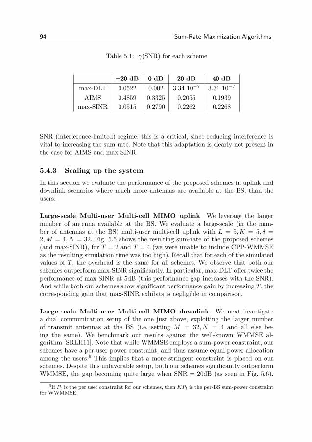
94 Sum-Rate Maximization Algorithms
Table 5.1: γ(SNR) for each scheme
−20−20−20 dB 000 dB 202020 dB 404040 dBmax-DLT 0.0522 0.002 3.34 10−7 3.31 10−7
AIMS 0.4859 0.3325 0.2055 0.1939max-SINR 0.0515 0.2790 0.2262 0.2268
SNR (interference-limited) regime: this is a critical, since reducing interference isvital to increasing the sum-rate. Note that this adaptation is clearly not present inthe case for AIMS and max-SINR.
5.4.3 Scaling up the systemIn this section we evaluate the performance of the proposed schemes in uplink anddownlink scenarios where much more antennas are available at the BS, than theusers.
Large-scale Multi-user Multi-cell MIMO uplink We leverage the largernumber of antenna available at the BS. We evaluate a large-scale (in the num-ber of antennas at the BS) multi-user multi-cell uplink with L = 5,K = 5, d =2,M = 4, N = 32. Fig. 5.5 shows the resulting sum-rate of the proposed schemes(and max-SINR), for T = 2 and T = 4 (we were unable to include CPP-WMMSEas the resulting simulation time was too high). Recall that for each of the simulatedvalues of T , the overhead is the same for all schemes. We observe that both ourschemes outperform max-SINR significantly. In particular, max-DLT offer twice theperformance of max-SINR at 5dB (this performance gap increases with the SNR).And while both our schemes show significant performance gain by increasing T , thecorresponding gain that max-SINR exhibits is negligible in comparison.
Large-scale Multi-user Multi-cell MIMO downlink We next investigatea dual communication setup of the one just above, exploiting the larger numberof transmit antennas at the BS (i.e, setting M = 32, N = 4 and all else be-ing the same). We benchmark our results against the well-known WMMSE al-gorithm [SRLH11]. Note that while WMMSE employs a sum-power constraint, ourschemes have a per-user power constraint, and thus assume equal power allocationamong the users.6 This implies that a more stringent constraint is placed on ourschemes. Despite this unfavorable setup, both our schemes significantly outperformWMMSE, the gap becoming quite large when SNR = 20dB (as seen in Fig. 5.6).
6If Pt is the per user constraint for our schemes, then KPt is the per-BS sum-power constraintfor WWMMSE.

5.4. Numerical Results 95
−10 −5 0 5 10 15 200
50
100
150
200
250
1/ σ2 (dB)
Su
m−
rate
(b
ps/H
z)
Sum−rate for M = 4, N = 32, L = 5, K = 5, d = 2, it = 4
max−DLT (T=4, Ω=400)
AIMS (T=4, Ω=400)
max−SINR (T=4, Ω=400)
max−SINR (T=2, Ω=200)
AIMS (T=2, Ω=200)
max−DLT (T=2, Ω=200)
Figure 5.5: Ergodic sum-rate for L = 5,K = 5,M = 4, N = 32, d = 2 (Uplink)
Note as well that the overhead of our proposed schemes, is half that of WMMSEas the latter requires feedback of the weights (refer to Sec. 5.3.4 for the overheadcalculations). Needless to say, the full-performance that WMMSE is expected todeliver, is reached after more iterations are performed. The reason behind this be-havior is the fast-converging nature of our algorithms, allowing them to reach agood operating point, in just 2 iterations. In the case of the max-DLT, this is turndue to the stream control feature of the non-homogeneous waterfilling.
5.4.4 Discussions
As mentioned earlier, the non-homogeneous waterfilling solution clearly shows thatstreams that have low SINR are turned-off, and power is only allocated to the onesthat exhibit relatively high SINR. This greatly speeds up the convergence of max-DLT, and allows it to achieve its required performance, with that limited numberof F-B iterations (e.g., 2). On the other hand, due to the large dimensions inherentto low-band mmWave systems (i.e., more antennas, cells, users) other benchmarkswill require more iterations to reach a similar performance. As for the overhead,our schemes are based on the framework of F-B iterations and result in minimaloverhead (the overhead consisting of uplink/downlink pilots only). However, otherschemes such as WMMSE and CCP-WMMSE require additional pilots and feed-back, and result in significantly higher overhead (as detailed in Sec. 5.3.4).

96 Sum-Rate Maximization Algorithms
1 2 3 4 5 6 7 80
20
40
60
80
100
120
140
160
180
200
220
T
Su
m−
rate
(b
ps/H
z)
max−DLT (Ω=100T)
WMMSE (Ω=200T)
AIMS w/RA (Ω=100T)
SNR=20dB
SNR=10dB
Figure 5.6: Ergodic sum-rate for L = 5,K = 5,M = 32, N = 4, d = 2 (Downlink)
5.5 Conclusion
In this chapter, we advocated the use of DLT bounds (as a lower bound on the sum-rate) and highlighted their significant advantage in yielding optimization problemsthat decouple at both the transmitters and receivers. More importantly, we pro-vided a generic solution for the latter, the so-called non-homogeneous waterfilling:we underlined its built-in stream-control feature, and its role in speeding up theconvergence. We proposed a distributed algorithm, max-DLT, that solves the latterproblem in a distributed manner. We later verified through simulations that ourproposed algorithms massively outperform other relevant benchmark algorithms(especially in interference-limited multi-user environments), for several communi-cation scenarios.
5.6 Appendix
5.6.1 Uniqueness of SVDThe proofs in this work rely on the central premise of mapping the problem into aseries of equivalent forms, where equivalence is ensured by the uniqueness of eachmapping [BV04]. One of the steps is rewrite the problem by mapping the variableinto its SVD form: for example, let maxXXX f(XXX) = tr(XXX†QQQXXX) and let XXX = UUUΣΣΣVVV †be the SVD of XXX. Generally speaking, the SVD is unique only up to rotationsof the left and right singular vectors, i.e., the actual SVD of XXX takes this form,
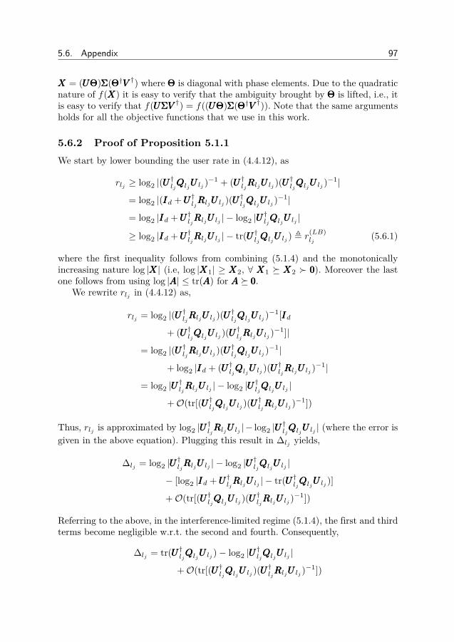
5.6. Appendix 97
XXX = (UUUΘΘΘ)ΣΣΣ(ΘΘΘ†VVV †) where ΘΘΘ is diagonal with phase elements. Due to the quadraticnature of f(XXX) it is easy to verify that the ambiguity brought by ΘΘΘ is lifted, i.e., itis easy to verify that f(UUUΣΣΣVVV †) = f((UUUΘΘΘ)ΣΣΣ(ΘΘΘ†VVV †)). Note that the same argumentsholds for all the objective functions that we use in this work.
5.6.2 Proof of Proposition 5.1.1We start by lower bounding the user rate in (4.4.12), as
rlj ≥ log2 |(UUU†ljQQQljUUU lj )
−1 + (UUU†ljRRRljUUU lj )(UUU†ljQQQljUUU lj )
−1|
= log2 |(IIId +UUU†ljRRRljUUU lj )(UUU†ljQQQljUUU lj )
−1|
= log2 |IIId +UUU†ljRRRljUUU lj | − log2 |UUU†ljQQQljUUU lj |
≥ log2 |IIId +UUU†ljRRRljUUU lj | − tr(UUU†ljQQQljUUU lj ) , r(LB)lj
(5.6.1)
where the first inequality follows from combining (5.1.4) and the monotonicallyincreasing nature log |XXX| (i.e, log |XXX1| ≥ XXX2, ∀ XXX1 XXX2 000). Moreover the lastone follows from using log |AAA| ≤ tr(AAA) for AAA 000.
We rewrite rlj in (4.4.12) as,
rlj = log2 |(UUU†ljRRRljUUU lj )(UUU
†ljQQQljUUU lj )
−1[IIId+ (UUU†ljQQQljUUU lj )(UUU
†ljRRRljUUU lj )−1]|
= log2 |(UUU†ljRRRljUUU lj )(UUU
†ljQQQljUUU lj )
−1|
+ log2 |IIId + (UUU†ljQQQljUUU lj )(UUU†ljRRRljUUU lj )−1|
= log2 |UUU†ljRRRljUUU lj | − log2 |UUU
†ljQQQljUUU lj |
+O(tr[(UUU†ljQQQljUUU lj )(UUU†ljRRRljUUU lj )−1])
Thus, rlj is approximated by log2 |UUU†ljRRRljUUU lj | − log2 |UUU
†ljQQQljUUU lj | (where the error is
given in the above equation). Plugging this result in ∆lj yields,
∆lj = log2 |UUU†ljRRRljUUU lj | − log2 |UUU
†ljQQQljUUU lj |
− [log2 |IIId +UUU†ljRRRljUUU lj | − tr(UUU†ljQQQljUUU lj )]
+O(tr[(UUU†ljQQQljUUU lj )(UUU†ljRRRljUUU lj )−1])
Referring to the above, in the interference-limited regime (5.1.4), the first and thirdterms become negligible w.r.t. the second and fourth. Consequently,
∆lj = tr(UUU†ljQQQljUUU lj )− log2 |UUU†ljQQQljUUU lj |
+O(tr[(UUU†ljQQQljUUU lj )(UUU†ljRRRljUUU lj )−1])
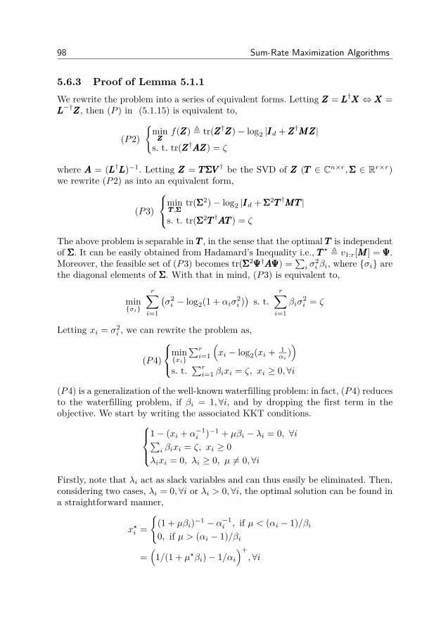
98 Sum-Rate Maximization Algorithms
5.6.3 Proof of Lemma 5.1.1We rewrite the problem into a series of equivalent forms. Letting ZZZ = LLL†XXX ⇔XXX =LLL−†ZZZ, then (P ) in (5.1.15) is equivalent to,
(P2)
minZZZ
f(ZZZ) , tr(ZZZ†ZZZ)− log2 |IIId +ZZZ†MMMZZZ|
s. t. tr(ZZZ†AAAZZZ) = ζ
where AAA = (LLL†LLL)−1. Letting ZZZ = TTTΣΣΣVVV † be the SVD of ZZZ (TTT ∈ Cn×r,ΣΣΣ ∈ Rr×r)we rewrite (P2) as into an equivalent form,
(P3)
minTTT ,ΣΣΣ
tr(ΣΣΣ2)− log2 |IIId + ΣΣΣ2TTT †MMMTTT |
s. t. tr(ΣΣΣ2TTT †AAATTT ) = ζ
The above problem is separable in TTT , in the sense that the optimal TTT is independentof ΣΣΣ. It can be easily obtained from Hadamard’s Inequality i.e., TTT ? , v1:r[MMM ] = ΨΨΨ.Moreover, the feasible set of (P3) becomes tr(ΣΣΣ2ΨΨΨ†AAAΨΨΨ) =
∑i σ
2i βi, where σi are
the diagonal elements of ΣΣΣ. With that in mind, (P3) is equivalent to,
minσi
r∑i=1
(σ2i − log2(1 + αiσ
2i ))s. t.
r∑i=1
βiσ2i = ζ
Letting xi = σ2i , we can rewrite the problem as,
(P4)
minxi
∑ri=1
(xi − log2(xi + 1
αi))
s. t.∑ri=1 βixi = ζ, xi ≥ 0,∀i
(P4) is a generalization of the well-known waterfilling problem: in fact, (P4) reducesto the waterfilling problem, if βi = 1,∀i, and by dropping the first term in theobjective. We start by writing the associated KKT conditions.
1− (xi + α−1i )−1 + µβi − λi = 0, ∀i∑
i βixi = ζ, xi ≥ 0λixi = 0, λi ≥ 0, µ 6= 0,∀i
Firstly, note that λi act as slack variables and can thus easily be eliminated. Then,considering two cases, λi = 0,∀i or λi > 0,∀i, the optimal solution can be found ina straightforward manner,
x?i =
(1 + µβi)−1 − α−1i , if µ < (αi − 1)/βi
0, if µ > (αi − 1)/βi
=(
1/(1 + µ?βi)− 1/αi)+,∀i

5.6. Appendix 99
where µ? is the unique root to
g(µ) ,r∑i=1
βi
(1/(1 + µβi)− 1/αi
)+− ζ
Note that g(µ) is monotonically decreasing, for µ > −1/(maxi βi), and µ? can befound using standard 1D search methods, such as bisection.
Thus, the optimal solution for (J1) is ZZZ? = ΨΨΨΣΣΣ?(where ΣΣΣ?(i,i) = √xi,∀i), andthat of (5.1.15) is XXX? = LLL−†ΨΨΨΣΣΣ?
5.6.4 Proof of Lemma 5.1.2It was shown in [Pri03] that the solution to (5.2.6) is given by, XXX? = LLL−†ΨΨΨ. Wenote that it can verified that this optimal solution is invariant to scaling, i.e.,q(XXX?ΣΣΣ) = q(XXX?), unitary rotation, i.e., q(XXX?VVV ) = q(XXX?), and q(XXX?SSS) = q(XXX?) forany SSS ∈ Cr×r that is non-singular. Thus the generic form of the solution is,
XXX? = LLL−†ΨΨΨ(ΣΣΣVVV †SSS) = LLL−†ΨΨΨVVV
where VVV is square and non-singular.


Chapter 6
Leakage Minimization Algorithms
In this chapter, we propose a low-overhead distributed schemes for transmit andreceive filter optimization. In line with the main design goals of this part ofthe thesis (Sect. 4.3.3), the proposed schemes in this chapter only require a
few forward-backward iterations, thus causing minimal communication overhead.For that purpose, we relax the well-known leakage minimization problem, and thenpropose two different filter update structures to solve the resulting non-convexproblem: though one leads to conventional full-rank filters, the other results inrank-deficient filters, that we exploit to gradually reduce the transmit and receivefilter rank, and greatly speed up the convergence. Furthermore, inspired from thedecoding of turbo codes, we propose a turbo-like structure to the algorithms, wherea separate inner optimization loop is run at each receiver (in addition to the mainforward-backward iteration). This is illustrated in Fig. 6.1. In that sense, the intro-duction of this turbo-like structure converts the communication overhead requiredby conventional methods to computational overhead at each receiver (a cheap re-source), allowing us to achieve the desired performance, under a minimal overheadconstraint. Finally, we show through comprehensive simulations that both proposedschemes hugely outperform the relevant benchmarks, especially for large system di-mensions. Although the algorithms and results in this Chapter are presented in thecontext of MIMO IC for simplicity, they are still applicable to both MIMO IBCand MIMO IMAC. The notation in this chapter deviates from the thesis notation(defined in Chap. 1), in the following aspect only λi[QQQ] denotes the ith eigenvalueof a Hermitian matrix QQQ ( assuming the eigenvalues are sorted in increasing order),
6.1 System Model and Problem Formulation
We hence start from the MIMO IBC signal model (presented in Chap. 4.2.1), werestate the leakage minimization problem as (Chap. 4.4.4),
min φ(UUU lj, VVV lj) =∑lj∈I tr(UUU
†
ljQQQljUUU lj )
s. t. UUU †ljUUU lj = IIId, VVV†
ljVVV lj = IIId, ∀lj ∈ L
(6.1.1)
101

102 Leakage Minimization Algorithms
Figure 6.1: Proposed Algorithm Structure, within the framework of F-B training
where we define the interference covariance matrix at receiver lj ∈ I as,
QQQlj =∑ik∈Iik 6=lj
(ρ/d)HHHk,ljVVV ikVVV†
ikHHH†k,lj (6.1.2)
and the interference covariance matrix at transmitter lj , as follows,
QQQlj =∑ik∈Iik 6=lj
HHH†j,ikUUU ikUUU†
ikHHHj,ik (6.1.3)
Recall that the above leakage minimization problem results in optimizing a lowerbound on the sum-rate - albeit a loose one (as shown in Chap. 4.4.4).
6.1.1 Problem FormulationNow that we have motivated the leakage minimization problem, we turn out atten-tion to devising an iterative algorithm for that purpose. As mentioned earlier, theschemes that we study in this work, fall under the category of distributed schemes,where each receiver / transmitter optimizes its filter, based on the estimated inter-ference covariance matrix. In other words, at the lth F-B iteration, after estimatingand updating its interference covariance matrix, QQQnlj ← QQQn+1
lj, receiver lj aims
to update its filter, UUUnlj ← UUUn+1lj
, such as to optimize some predetermined met-ric (interference leakage, mean-squared error, sum-rate, etc...). The F-B iterationstructure was first applied within the context of IA, in the distributed IA algorithm
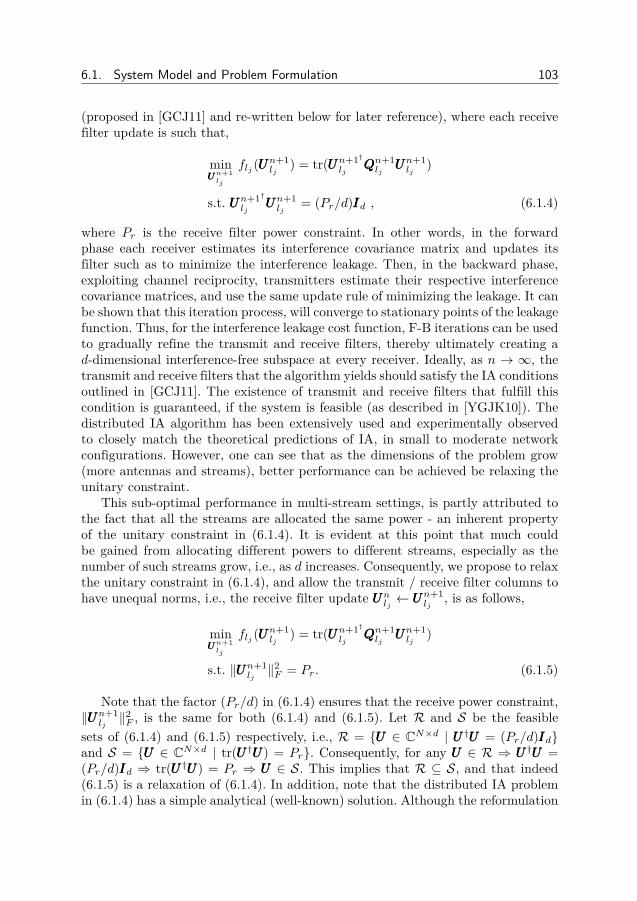
6.1. System Model and Problem Formulation 103
(proposed in [GCJ11] and re-written below for later reference), where each receivefilter update is such that,
minUUUn+1lj
flj (UUUn+1lj
) = tr(UUUn+1†lj
QQQn+1lj
UUUn+1lj
)
s.t. UUUn+1†lj
UUUn+1lj
= (Pr/d)IIId , (6.1.4)
where Pr is the receive filter power constraint. In other words, in the forwardphase each receiver estimates its interference covariance matrix and updates itsfilter such as to minimize the interference leakage. Then, in the backward phase,exploiting channel reciprocity, transmitters estimate their respective interferencecovariance matrices, and use the same update rule of minimizing the leakage. It canbe shown that this iteration process, will converge to stationary points of the leakagefunction. Thus, for the interference leakage cost function, F-B iterations can be usedto gradually refine the transmit and receive filters, thereby ultimately creating ad-dimensional interference-free subspace at every receiver. Ideally, as n → ∞, thetransmit and receive filters that the algorithm yields should satisfy the IA conditionsoutlined in [GCJ11]. The existence of transmit and receive filters that fulfill thiscondition is guaranteed, if the system is feasible (as described in [YGJK10]). Thedistributed IA algorithm has been extensively used and experimentally observedto closely match the theoretical predictions of IA, in small to moderate networkconfigurations. However, one can see that as the dimensions of the problem grow(more antennas and streams), better performance can be achieved be relaxing theunitary constraint.
This sub-optimal performance in multi-stream settings, is partly attributed tothe fact that all the streams are allocated the same power - an inherent propertyof the unitary constraint in (6.1.4). It is evident at this point that much couldbe gained from allocating different powers to different streams, especially as thenumber of such streams grow, i.e., as d increases. Consequently, we propose to relaxthe unitary constraint in (6.1.4), and allow the transmit / receive filter columns tohave unequal norms, i.e., the receive filter update UUUnlj ← UUUn+1
lj, is as follows,
minUUUn+1lj
flj (UUUn+1lj
) = tr(UUUn+1†lj
QQQn+1lj
UUUn+1lj
)
s.t. ‖UUUn+1lj‖2F = Pr. (6.1.5)
Note that the factor (Pr/d) in (6.1.4) ensures that the receive power constraint,‖UUUn+1
lj‖2F , is the same for both (6.1.4) and (6.1.5). Let R and S be the feasible
sets of (6.1.4) and (6.1.5) respectively, i.e., R = UUU ∈ CN×d | UUU†UUU = (Pr/d)IIIdand S = UUU ∈ CN×d | tr(UUU†UUU) = Pr. Consequently, for any UUU ∈ R ⇒ UUU†UUU =(Pr/d)IIId ⇒ tr(UUU†UUU) = Pr ⇒ UUU ∈ S. This implies that R ⊆ S, and that indeed(6.1.5) is a relaxation of (6.1.4). In addition, note that the distributed IA problemin (6.1.4) has a simple analytical (well-known) solution. Although the reformulation
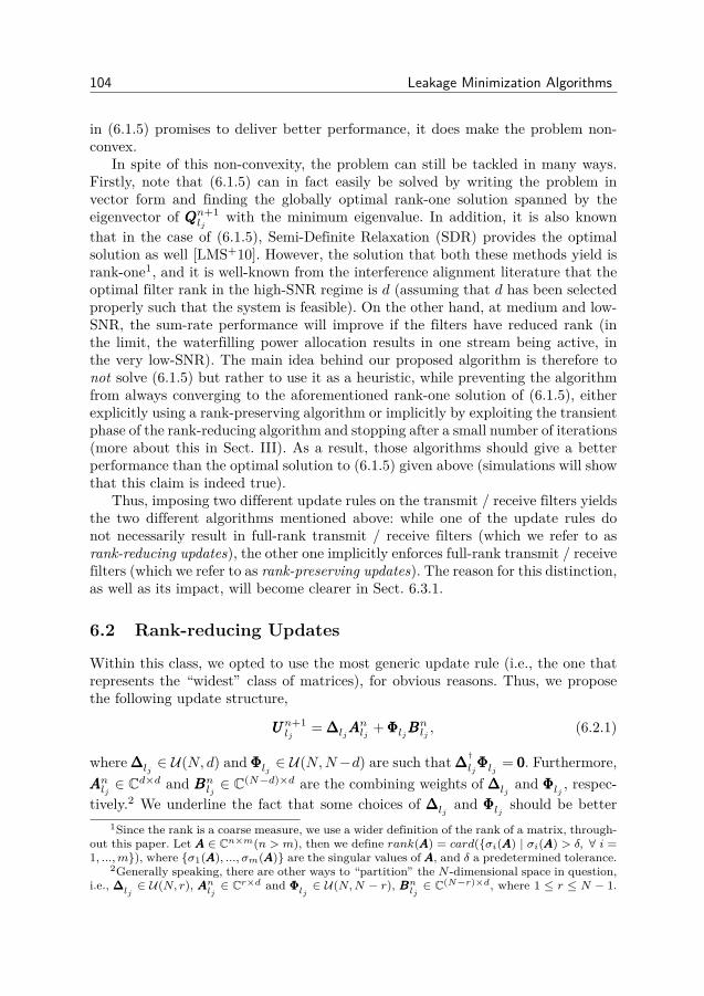
104 Leakage Minimization Algorithms
in (6.1.5) promises to deliver better performance, it does make the problem non-convex.
In spite of this non-convexity, the problem can still be tackled in many ways.Firstly, note that (6.1.5) can in fact easily be solved by writing the problem invector form and finding the globally optimal rank-one solution spanned by theeigenvector of QQQn+1
ljwith the minimum eigenvalue. In addition, it is also known
that in the case of (6.1.5), Semi-Definite Relaxation (SDR) provides the optimalsolution as well [LMS+10]. However, the solution that both these methods yield isrank-one1, and it is well-known from the interference alignment literature that theoptimal filter rank in the high-SNR regime is d (assuming that d has been selectedproperly such that the system is feasible). On the other hand, at medium and low-SNR, the sum-rate performance will improve if the filters have reduced rank (inthe limit, the waterfilling power allocation results in one stream being active, inthe very low-SNR). The main idea behind our proposed algorithm is therefore tonot solve (6.1.5) but rather to use it as a heuristic, while preventing the algorithmfrom always converging to the aforementioned rank-one solution of (6.1.5), eitherexplicitly using a rank-preserving algorithm or implicitly by exploiting the transientphase of the rank-reducing algorithm and stopping after a small number of iterations(more about this in Sect. III). As a result, those algorithms should give a betterperformance than the optimal solution to (6.1.5) given above (simulations will showthat this claim is indeed true).
Thus, imposing two different update rules on the transmit / receive filters yieldsthe two different algorithms mentioned above: while one of the update rules donot necessarily result in full-rank transmit / receive filters (which we refer to asrank-reducing updates), the other one implicitly enforces full-rank transmit / receivefilters (which we refer to as rank-preserving updates). The reason for this distinction,as well as its impact, will become clearer in Sect. 6.3.1.
6.2 Rank-reducing Updates
Within this class, we opted to use the most generic update rule (i.e., the one thatrepresents the “widest” class of matrices), for obvious reasons. Thus, we proposethe following update structure,
UUUn+1lj
= ∆∆∆ljAAAnlj + ΦΦΦljBBB
nlj , (6.2.1)
where ∆∆∆lj∈ U(N, d) and ΦΦΦlj ∈ U(N,N−d) are such that ∆∆∆†ljΦΦΦlj = 000. Furthermore,
AAAnlj ∈ Cd×d and BBBnlj ∈ C(N−d)×d are the combining weights of ∆∆∆ljand ΦΦΦlj , respec-
tively.2 We underline the fact that some choices of ∆∆∆ljand ΦΦΦlj should be better
1Since the rank is a coarse measure, we use a wider definition of the rank of a matrix, through-out this paper. Let AAA ∈ Cn×m(n > m), then we define rank(AAA) = card(σi(AAA) | σi(AAA) > δ, ∀ i =1, ...,m), where σ1(AAA), ..., σm(AAA) are the singular values of AAA, and δ a predetermined tolerance.
2Generally speaking, there are other ways to “partition” the N -dimensional space in question,i.e., ∆∆∆lj
∈ U(N, r), AAAnlj∈ Cr×d and ΦΦΦlj
∈ U(N,N − r), BBBnlj∈ C(N−r)×d, where 1 ≤ r ≤ N − 1.
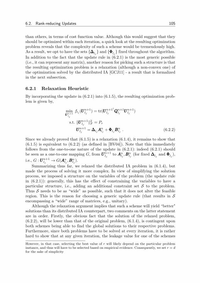
6.2. Rank-reducing Updates 105
than others, in terms of cost function value. Although this would suggest that theyshould be optimized within each iteration, a quick look at the resulting optimizationproblem reveals that the complexity of such a scheme would be tremendously high.As a result, we opt to have the sets ∆∆∆lj
and ΦΦΦlj fixed throughout the algorithm.In addition to the fact that the update rule in (6.2.1) is the most generic possible(i.e., it can represent any matrix), another reason for picking such a structure is thatthe resulting optimization problem is a relaxation (although a non-convex one) ofthe optimization solved by the distributed IA [GCJ11] - a result that is formalizedin the next subsection.
6.2.1 Relaxation HeuristicBy incorporating the update in (6.2.1) into (6.1.5), the resulting optimization prob-lem is given by,
minUUUn+1lj
flj (UUUn+1lj
) = tr(UUUn+1†lj
QQQn+1lj
UUUn+1lj
)
s.t. ‖UUUn+1lj‖2F = Pr
UUUn+1lj
= ∆∆∆ljAAAnlj + ΦΦΦljBBB
nlj . (6.2.2)
Since we already proved that (6.1.5) is a relaxation (6.1.4), it remains to show that(6.1.5) is equivalent to (6.2.2) (as defined in [BV04]). Note that this immediatelyfollows from the one-to-one nature of the update in (6.2.1): indeed (6.2.1) shouldbe seen as a one-to-one mapping G, from UUUn+1
ljto AAAnlj ,BBB
nlj(for fixed ∆∆∆lj
and ΦΦΦlj ),i.e., G : UUUn+1
lj→ G(AAAnlj ,BBB
nlj
).Summarizing thus far, we relaxed the distributed IA problem in (6.1.4), but
made the process of solving it more complex. In view of simplifying the solutionprocess, we imposed a structure on the variables of the problem (the update rulein (6.2.1)): generally, this has the effect of constraining the variables to have aparticular structure, i.e., adding an additional constraint set S to the problem.Thus S needs to be as “wide” as possible, such that it does not alter the feasibleregion. This is the reason for choosing a generic update rule (that results in Sencompassing a “wide” range of matrices, e.g., unitary).
Although the relaxation argument implies that such a scheme will yield “better"solutions than its distributed IA counterpart, two comments on the latter statementare in order. Firstly, the obvious fact that the solution of the relaxed problem,(6.2.2), will be lower than that of the original problem, (6.1.4), is contingent uponboth schemes being able to find the global solutions to their respective problems.Furthermore, since both problems have to be solved at every iteration, it is ratherhard to show that at any given iteration, the leakage value for one of the schemes
However, in that case, selecting the best value of r will likely depend on the particular probleminstance, and thus will have to be selected based on empirical evidence. Consequently, we set r = dfor the sake of simplicity
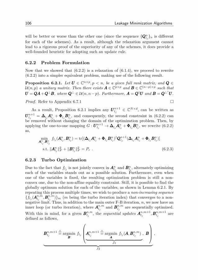
106 Leakage Minimization Algorithms
will be better or worse than the other one (since the sequence QQQnljn is differentfor each of the schemes). As a result, although the relaxation argument cannotlead to a rigorous proof of the superiority of any of the schemes, it does provide awell-founded heuristic for adopting such an update rule.
6.2.2 Problem FormulationNow that we showed that (6.2.2) is a relaxation of (6.1.4), we proceed to rewrite(6.2.2) into a simpler equivalent problem, making use of the following result.
Proposition 6.2.1. Let UUU ∈ Cn×p, p < n, be a given full rank matrix, and QQQ ∈U(n, p) a unitary matrix. Then there exists AAA ∈ Cp×p and BBB ∈ C(n−p)×p such thatUUU = QAQAQA+QQQ⊥BBB, where QQQ⊥ ∈ U(n, n− p). Furthermore, AAA = QQQ†UUU and BBB = QQQ⊥
†UUU .
Proof. Refer to Appendix 6.7.1
As a result, Proposition 6.2.1 implies any UUUn+1lj
∈ CN×d, can be written asUUUn+1lj
= ∆∆∆ljAAAnlj + ΦΦΦljBBB
nlj, and consequently, the second constraint in (6.2.2) can
be removed without changing the domain of the optimization problem. Then, byapplying the one-to-one mapping G : UUUn+1
lj→ ∆∆∆lj
AAAnlj + ΦΦΦljBBBnlj, we rewrite (6.2.2)
as,
minAAAnlj,BBBnlj
flj (AAAnlj ,BBBnlj ) = tr[(∆∆∆ljAAA
nlj + ΦΦΦljBBB
nlj )†QQQn+1
lj(∆∆∆ljAAA
nlj + ΦΦΦljBBB
nlj )]
s.t. ‖AAAnlj‖2F + ‖BBBnlj‖
2F = Pr . (6.2.3)
6.2.3 Turbo OptimizationDue to the fact that flj is not jointly convex in AAAnlj and BBB
nlj, alternately optimizing
each of the variables stands out as a possible solution. Furthermore, even whenone of the variables is fixed, the resulting optimization problem is still a non-convex one, due to the non-affine equality constraint. Still, it is possible to find theglobally optimum solution for each of the variables, as shown in Lemma 6.2.1. Byrepeating this process multiple times, we wish to produce a non-increasing sequenceflj (AAA
n,mlj
,BBBn,mlj )m (m being the turbo iteration index) that converges to a non-negative limit. Thus, in addition to the main outer F-B iteration, n, we now have aninner loop (or turbo iteration), where AAAn,mlj and BBBn,mlj are sequentially optimized.With this in mind, for a given BBBn,mlj , the sequential updates AAAn,m+1
lj,BBBn,m+1
ljare
defined as follows,
BBBn,m+1lj
4= argminBBB
flj
AAAn,m+1lj
4= argminAAA
flj (AAA,BBBn,mlj
)︸ ︷︷ ︸J1
, BBB
︸ ︷︷ ︸
J2
,

6.2. Rank-reducing Updates 107
where the inner optimization problems are elaborated below,
(J1) : AAAn,m+1lj
= argminAAA
flj (AAA,BBBn,mlj
)
s. t. h1(AAA) = ‖AAA‖2F + ‖BBBn,mlj ‖2F − Pr = 0 ,
(J2) : BBBn,m+1lj
= argminBBB
flj (AAAn,m+1lj
,BBB)
s. t. h2(BBB) = ‖BBB‖2F + ‖AAAn,m+1lj
‖2F − Pr = 0 .
Remark 6.1. Both (J1) and (J2) are non-convex due to the quadratic equalityconstraint. Note that applying convex relaxation by replacing the equality by aninequality (thus forming a convex superset) will not help: indeed one can show inthat that the sequences of optimal updates within the turbo iteration, are suchthat AAAn,mlj m → 000 and BBBn,mlj m → 000 (consequently, UUUn+1
lj= 000 , implying that the
algorithm converges to a point that does not necessarily correspond to stationarypoints of the leakage function).
The following lemma provides the solution to the different subproblems of ourproposed algorithms.
Lemma 6.2.1. Consider the following non-convex quadratic program,
minXXX
f(XXX) = tr[(γ1ΘΘΘ + γ2TTTXXX)†QQQ(γ1ΘΘΘ + γ2TTTXXX)]
s. t. h(XXX) = ‖XXX‖2F − ζ = 0 , ζ > 0 , (6.2.4)
where QQQ 000 , ΘΘΘ 6= 000 , 0 ≤ γ1 , γ2 ≤ 1. Then, the (globally optimum) solution XXX?
is given byXXX?(µ?) = −γ1γ2
(γ2
2 TTT†QQQTTT + µ?III
)−1TTT †QQQΘΘΘ (6.2.5)
where µ? is the unique solution to
‖XXX?(µ)‖2F = ζ
in the interval −γ22 λ1[TTT †QQQTTT ] < µ < γ1γ2‖ΘΘΘ†QQQTTT‖F /
√ζ. Moreover, ‖XXX?(µ)‖2F is
monotonically decreasing in µ, for µ > −γ22 λ1[TTT †QQQTTT ].
Proof. Refer to Appendix 6.7.2.
Though it might seem that (6.1.5) can be solved using Lemma 6.2.1, i.e., bysetting ΘΘΘ = 000, this does make the necessary and sufficient conditions inconsistent(refer to Appendix 6.7.2). On the other hand, it becomes clear at this point that (J1)is a special case of (6.2.4), by letting XXX = AAA, ΘΘΘ = ΦΦΦljBBB
n,mlj
, TTT = ∆∆∆lj, γ1 = γ2 = 1,
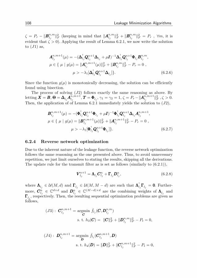
108 Leakage Minimization Algorithms
ζ = Pr − ‖BBBn,mlj ‖2F (keeping in mind that ‖AAAn,mlj ‖
2F + ‖BBBn,mlj ‖
2F = Pr , ∀m, it is
evident that ζ > 0). Applying the result of Lemma 6.2.1, we now write the solutionto (J1) as,
AAAn,m+1lj
(µ) = −(∆∆∆†
ljQQQn+1lj
∆∆∆lj + µIII)−1∆∆∆†
ljQQQn+1lj
ΦΦΦljBBBn,mlj
,
µ ∈ µ | g(µ) = ‖AAAn,m+1lj
(µ)‖2F + ‖BBBn,mlj ‖2F − Pr = 0 ,
µ > −λ1[∆∆∆†
ljQQQn+1lj
∆∆∆lj ]. (6.2.6)
Since the function g(µ) is monotonically decreasing, the solution can be efficientlyfound using bisection.
The process of solving (J2) follows exactly the same reasoning as above. BylettingXXX = BBB, ΘΘΘ = ∆∆∆lj
AAAn,m+1lj
, TTT = ΦΦΦlj , γ1 = γ2 = 1, ζ = Pr−‖AAAn,m+1lj
‖2F , ζ > 0.Then, the application of of Lemma 6.2.1 immediately yields the solution to (J2),
BBBn,m+1lj
(µ) = −(ΦΦΦ†
ljQQQn+1lj
ΦΦΦlj + µIII)−1ΦΦΦ†
ljQQQn+1lj
∆∆∆ljAAAn,m+1lj
,
µ ∈ µ | g(µ) = ‖BBBn,m+1lj
(µ)‖2F + ‖AAAn,m+1lj
‖2F − Pr = 0 ,
µ > −λ1[ΦΦΦ†
ljQQQn+1lj
ΦΦΦlj ]. (6.2.7)
6.2.4 Reverse network optimization
Due to the inherent nature of the leakage function, the reverse network optimizationfollows the same reasoning as the one presented above. Thus, to avoid unnecessaryrepetition, we just limit ourselves to stating the results, skipping all the derivations.The update rule for the transmit filter as is set as follows (similarly to (6.2.1)),
VVV n+1lj
= ΛΛΛljCCCnlj + ΓΓΓljDDD
nlj , (6.2.8)
where ΛΛΛlj ∈ U(M,d) and ΓΓΓlj ∈ U(M,M − d) are such that ΛΛΛ†ljΓΓΓlj = 000. Further-more, CCCnlj ∈ Cd×d and DDDn
lj∈ C(M−d)×d are the combining weights of ΛΛΛlj and
ΓΓΓlj , respectively. Then, the resulting sequential optimization problems are given asfollows,
(J3) : CCCn,m+1lj
= argminCCC
flj (CCC,DDDn,mlj
)
s. t. h3(CCC) = ‖CCC‖2F + ‖DDDn,mlj‖2F − Pt = 0,
(J4) : DDDn,m+1lj
= argminDDD
flj (CCCn,m+1lj
,DDD)
s. t. h4(DDD) = ‖DDD‖2F + ‖CCCn,m+1lj
‖2F − Pt = 0,

6.2. Rank-reducing Updates 109
where Pt is the transmit filter power constraint, and flj , the leakage at transmitterlj , is given by
flj (CCCnlj ,DDDnlj ) = tr(VVV n+1†
ljQQQn+1lj
VVV n+1lj
)
= tr[(ΛΛΛljCCCnlj + ΓΓΓljDDD
nlj )†QQQn+1
lj(ΛΛΛljCCC
nlj + ΓΓΓljDDD
nlj )].
Again, the same block coordinate descent structure can be employed to optimizethe weight matricesCCCnlj andDDD
nlj. Using the same reasoning as earlier, one can obtain
the optimal updates, using the result of Lemma 6.2.1, to yield,
CCCn,m+1lj
(µ) = −(ΛΛΛ†
lj QQQn+1lj
ΛΛΛlj + µIII)−1ΛΛΛ†
lj QQQn+1lj
ΓΓΓljDDDn,mlj
,
µ ∈ µ | g(µ) = ‖CCCn,m+1lj
(µ)‖2F + ‖DDDn,mlj‖2F − Pt = 0 ,
µ > −λ1[ΛΛΛ†
lj QQQn+1lj
ΛΛΛlj ], (6.2.9)
DDDn,m+1lj
(µ) = −(ΓΓΓ†
lj QQQn+1lj
ΓΓΓlj + µIII)−1ΓΓΓ†
lj QQQn+1lj
ΛΛΛljCCCn,m+1lj
,
µ ∈ µ | g(µ) = ‖DDDn,m+1lj
(µ)‖2F + ‖CCCn,m+1lj
‖2F − Pt = 0 ,
µ > −λ1[ΓΓΓ†
lj QQQn+1lj
ΓΓΓlj ]. (6.2.10)
The resulting algorithm, Iteratively Weighted Updates with Rank Reducing updates(IWU-RR) is shown in Algorithm 5.
Algorithm 5 Iterative Weight Update with Rank-Reduction (IWU-RR)T : number of F-B iterations, I : number of turbo iterationsfor n = 0, 1, ..., T − 1 do
// forward network optimizationUpdate receiver interference covariance matrixfor m = 0, 1, ..., I − 1 do
Compute AAAn,m+1lj
lj in (6.2.6), BBBn,m+1lj
lj in (6.2.7)end forCheck rank and perform rank-reduction (Remark 6.2)Update receive filter in (6.2.1)// reverse network optimization
Update transmitter interference covariance matrixfor m = 0, 1, ..., I − 1 do
Compute CCCn,m+1lj
lj in (6.2.9), DDDn,m+1lj
lj in (6.2.10)end forCheck rank and perform rank-reduction (Remark 6.2)Update transmit precoder in (6.2.8)
end for

110 Leakage Minimization Algorithms
Remark 6.2. If the weight combining matrices at the output of the turbo iteration(for, say, the receive filter update) are rank deficient, then resulting receive filter isrank deficient as well. The rank-reduction process is done by eliminating linearlydependent columns of AAAn,mlj and BBBn,mlj , and appropriately scaling each of them, tofulfill the power constraint.
6.2.5 Convergence AnalysisAs shown earlier, although the problem solved within the turbo iteration is a non-convex one, i.e., (6.2.3), we can still show that the application of the updates forAAAn,m+1lj
and BBBn,m+1lj
(given in (6.2.6) and (6.2.7), respectively), cannot increase theleakage at each receiver.
Theorem 6.2.1. For fixed VVV n+1ljlj , the leakage within the receiver turbo itera-
tion is non-increasing, i.e. the sequence flj (AAAn,mlj
,BBBn,mlj )m is non-increasing, andconverges to a non-negative limit fn,stlj
≥ 0, where AAAn,m+1lj
and BBBn,m+1lj
are givenin (6.2.6) and (6.2.7).
Proof. The proof immediately follows from showing that for a fixed F-B iterationnumber l, the following holds,
flj (AAAn,m+1lj
,BBBn,m+1lj
)(b)≤ flj (AAA
n,m+1lj
,BBBn,mlj )(a)≤ flj (AAA
n,mlj
,BBBn,mlj ),∀m. (6.2.11)
Note that (a) follows immediately from the definition and solution of (J1). Con-sequently, the application of the update AAAn,mlj ← AAAn,m+1
lj, given by (6.2.6), cannot
increase the cost function. Similarly, points that satisfy (6.2.7) mimimize (J2) (asshown by Lemma 6.2.1). Thus, the update BBBn,mlj ← BBBn,m+1
ljgiven in (6.2.7) cannot
increase the cost function, and (b) follows. Therefore, the sequence flj (AAAn,mlj
,BBBn,mlj )mis non-increasing, and since the leakage function is non-negative, we conclude thatflj (AAA
n,mlj
,BBBn,mlj )m converges to some non-negative limit fn,stlj.
With this in mind, not only does Theorem 6.2.1 establish the convergence of theturbo iteration to some limit, but also that the leakage is non-increasing with each ofthe updates (as immediately seen from (6.2.11)). Although Theorem 6.2.1 shows theconvergence of the turbo iteration, to some limit, one cannot claim that this limitcorresponds to a stationary point of the function, because the variables in (6.2.3) arecoupled [RHL12]. Moreover, recall that we do not wish our algorithm to convergeto stationary points of the leakage function since the latter correspond to rank-one solutions (following the discussion in Sect. II-B). Consequently, showing theconvergence of the block coordinate descent method to stationary points becomesmuch less critical in our case, as long as we can establish the non-increasing natureof the leakage. In addition, it is not hard to see that exactly the same reasoningcan be used to extrapolate the result of Theorem 6.2.1 to show that the updatesfor the transmit filter weights (given in (6.2.9) and (6.2.10)), can only decrease the

6.3. Rank-Preserving Updates 111
leakage at the given transmitter, and thus establishing the convergence of the turboiteration for the transmit filter weights.
6.2.6 Convergence to lower-rank solutionsFor convenience, we define T as the maximum number of F-B iterations, and Ias the maximum number of turbo iterations, for our algorithm. Strong (empirical)evidence suggests that the proposed algorithm will gradually reduce the transmit /receive filter rank, and converge to rank-one solutions, as T, I → ∞. As a result,operating the algorithm with large values of T, I will result in a multiplexing gainof 1 degree-of-freedom per user (highly suboptimal especially if multistream trans-mission is desired). Conversely, by allowing the algorithm to gradually reduce therank of a given transmit / receive filter, we exploit the “transient phase” of thisalgorithm stopping before convergence to rank-one solutions (i.e. for small values ofT, I). In addition, recall that reducing the transmit / receive filter rank also reducesthe dimension of the interference that is caused to other receivers (this is benefi-cial in the interference-limited regime): this makes the alignment of interference“easier” and greatly speeds up the convergence. Note as well that although havingsmall values of T, I is extremely desirable (the associated communication and com-putational overhead will be relatively low), having them too small will evidentlyresult in poor performance, e.g., T = 0, I = 0. This does suggest the existence ofa trade-off on T and I, between the performance and overhead. Unfortunately, amathematical characterization of the latter reveals to be impossible, and we willrely on empirical evidence to select them.
6.3 Rank-Preserving Updates
6.3.1 Proposed Update Rule and Problem FormulationAn inherent consequence of the coupled nature of the weight updates for AAAnlj andBBBnlj , i.e., (6.2.6) and (6.2.7) (as well as the turbo-like structure of the algorithm),is the fact that if any of the latter are rank-deficient, then the other one will berank-deficient as well. Moreover, imposing an explicit rank constraint would makethe problem extremely hard to solve (since most rank-constrained problems areNP-hard). Alternately, one way to have the algorithm yield full-rank solutions, isto use another update rule (shown below) where this effect is absent, i.e.,
UUUn+1lj
=√
1− βn2ljUUUnlj + βnlj∆∆∆
nljZZZ
nlj , 0 ≤ βnlj ≤ 1, (6.3.1)
where ∆∆∆nlj∈ U(N,N − d) is such that ∆∆∆n
lj⊆ (UUUnlj )
⊥, ZZZnlj ∈ C(N−d)×d is thecombining weight matrix for the receiver update, and βnlj is the step size for thereceive filter update. Note that due to the dependence of the update on the currentreceive filter, UUUnlj , it is easy to verify that UUUn+1
ljis full rank, if UUUnlj is. In addition, if

112 Leakage Minimization Algorithms
both UUUnlj and ZZZnlj satisfy the power constraint, i.e., ‖UUUnlj‖2F = Pr and ‖ZZZnlj‖
2F = Pr,
then ‖UUUn+1lj‖2F = Pr.
Similarly to (6.2.2), by incorporating the above update structure, the resultingoptimization problem at each receiver is stated as follows,
minUUUn+1lj
flj (UUUn+1lj
) = tr(UUUn+1†lj
QQQn+1lj
UUUn+1lj
)
s.t. ‖UUUn+1lj‖2F = Pr
UUUn+1lj
=√
1− βn2ljUUUnlj + βnlj∆∆∆
nljZZZ
nlj . (6.3.2)
A few comments are in order at this point regarding the similarities and funda-mental differences between the rank-reducing update proposed earlier, and therank-preserving update above. Given that both result in non-convex optimizationproblems, they both rely on a coordinate descent approach to optimize each oftheir respective variables. In addition, it is clear that the rank-reducing update in(6.2.1) is more generic than the rank-preserving update in (6.3.1). As a result, therelaxation argument that was put forth to motivate the use of the update in (6.2.1)(Sect. 6.2.1), no longer holds here. Furthermore, both algorithms have exactly thesame structure: in that sense, after updating its interference covariance matrix, re-ceiver lj wishes to optimize both its combining weight and step-size, i.e. βnlj andZZZnlj , such as to minimize the resulting interference leakage at the next iteration.Plugging (6.3.1) into (6.3.2) yields the cost function at receiver lj ,
flj (βnlj ,ZZZnlj ) = (1− βn
2
lj )tr(UUUn†
lj QQQn+1lj
UUUnlj ) + βn2
lj tr(ZZZn†
lj ∆∆∆n†
lj QQQn+1lj
∆∆∆nljZZZ
nlj )
+ 2βnlj√
1− βn2ljRe[tr(UUUn
†
lj QQQn+1lj
∆∆∆nljZZZ
nlj )]. (6.3.3)
6.3.2 Inner OptimizationAgain, we will use block coordinate descent to mitigate the non-convexity of (6.3.3),implying that receiver lj optimizes both its weight combining matrix and stepsize (ZZZnlj and βnlj ), alternately and sequentially, within the turbo iteration, to pro-duce a non-increasing sequence flj (β
n,mlj
,ZZZn,mlj )m that will converge to some non-negative limit. Thus, given βn,mlj at themth turbo iteration, the sequential updatesZZZn,m+1lj
and βn,m+1lj
are chosen, as follows,
βn,m+1lj
4= argminβ
flj
β, ZZZn,m+1lj
4= argminZZZ
flj (βn,mlj
,ZZZ)︸ ︷︷ ︸K1
︸ ︷︷ ︸
K2
,
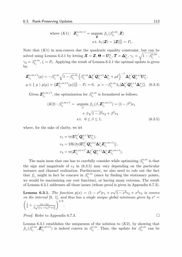
6.3. Rank-Preserving Updates 113
where (K1) : ZZZn,m+1lj
= argminZZZ
flj (βn,mlj
,ZZZ)
s.t. h1(ZZZ) = ‖ZZZ‖2F = Pr.
Note that (K1) in non-convex due the quadratic equality constraint, but can besolved using Lemma 6.2.1 by letting XXX = ZZZ, ΘΘΘ = UUUnlj , TTT = ∆∆∆n
lj, γ1 =
√1− βn,mlj ,
γ2 = βn,mlj , ζ = Pr. Applying the result of Lemma 6.2.1 the optimal update is givenby,
ZZZn,m+1lj
(µ) = −βn,mlj√
1− βn,mlj(βn,mlj ∆∆∆n†
lj QQQn+1lj
∆∆∆nlj + µI
)−1∆∆∆n†
lj QQQn+1lj
UUUnlj ,
µ ∈ µ | g(µ) = ‖ZZZn,m+1lj
(µ)‖2F − Pr = 0, µ > −βn,mlj λ1[∆∆∆n†
lj QQQn+1lj
∆∆∆nlj ]. (6.3.4)
Given ZZZn,m+1lj
, the optimization for βn,mlj is formulated as follows,
(K2) : βn,m+1lj
= argminβ
flj (β,ZZZn,m+1lj
) = (1− β2)e1
+ β√
1− β2e2 + β2e3
s.t. 0 ≤ β ≤ 1, (6.3.5)
where, for the sake of clarity, we let
e1 = tr(UUUn†
lj QQQn+1lj
UUUnlj ),
e2 = 2Re[tr(UUUn†
lj QQQn+1lj
∆∆∆nljZZZ
n,m+1lj
)],
e3 = tr(ZZZn,m+1†lj
∆∆∆n†
lj QQQn+1lj
∆∆∆nljZZZ
n,m+1lj
).
The main issue that one has to carefully consider while optimizing βn,mlj is thatthe sign and magnitude of e2 in (6.3.5) may vary depending on the particularinstance and channel realization. Furthermore, we also need to rule out the factthat flj might in fact be concave in βn,mlj (since by finding the stationary points,we would be maximizing our cost function), or having many extrema. The resultof Lemma 6.3.1 addresses all those issues (whose proof is given in Appendix 6.7.3).
Lemma 6.3.1. The function p(x) = (1 − x2)e1 + x√
1− x2e2 + x2e3 is convexon the interval [0, 1], and thus has a single unique global minimum given by x∗ =(
12 + e1−e3
2√
(e1−e3)2+e22
)1/2.
Proof. Refer to Appendix 6.7.3.
Lemma 6.3.1 establishes the uniqueness of the solution to (K2), by showing thatflj (β
n,mlj
,ZZZn,m+1lj
) is indeed convex in βn,mlj . Thus, the update for βn,mlj can be
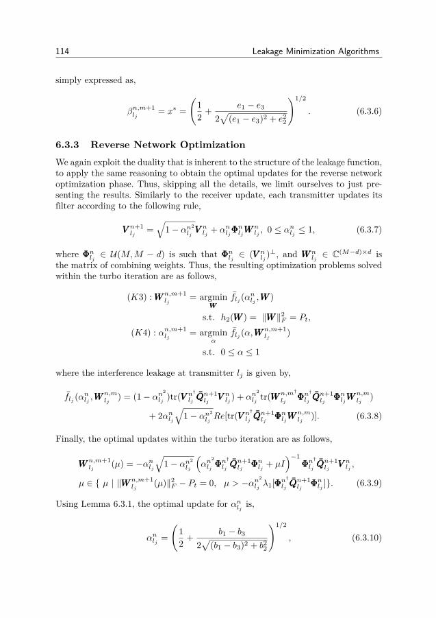
114 Leakage Minimization Algorithms
simply expressed as,
βn,m+1lj
= x∗ =(
12 + e1 − e3
2√
(e1 − e3)2 + e22
)1/2
. (6.3.6)
6.3.3 Reverse Network OptimizationWe again exploit the duality that is inherent to the structure of the leakage function,to apply the same reasoning to obtain the optimal updates for the reverse networkoptimization phase. Thus, skipping all the details, we limit ourselves to just pre-senting the results. Similarly to the receiver update, each transmitter updates itsfilter according to the following rule,
VVV n+1lj
=√
1− αn2ljVVV nlj + αnljΦΦΦ
nljWWW
nlj , 0 ≤ αnlj ≤ 1, (6.3.7)
where ΦΦΦnlj ∈ U(M,M − d) is such that ΦΦΦnlj ∈ (VVV nlj )⊥, and WWWn
lj∈ C(M−d)×d is
the matrix of combining weights. Thus, the resulting optimization problems solvedwithin the turbo iteration are as follows,
(K3) : WWWn,m+1lj
= argminWWW
flj (αnlj ,WWW )
s.t. h2(WWW ) = ‖WWW‖2F = Pt,
(K4) : αn,m+1lj
= argminα
flj (α,WWWn,m+1lj
)
s.t. 0 ≤ α ≤ 1
where the interference leakage at transmitter lj is given by,
flj (αnlj ,WWWn,mlj
) = (1− αn2
lj )tr(VVV n†
lj QQQn+1lj
VVV nlj ) + αn2
lj tr(WWWn,m†
ljΦΦΦn†
lj QQQn+1lj
ΦΦΦnljWWWn,mlj
)
+ 2αnlj√
1− αn2ljRe[tr(VVV n
†
lj QQQn+1lj
ΦΦΦnljWWWn,mlj
)]. (6.3.8)
Finally, the optimal updates within the turbo iteration are as follows,
WWWn,m+1lj
(µ) = −αnlj√
1− αn2lj
(αn
2
lj ΦΦΦn†
lj QQQn+1lj
ΦΦΦnlj + µI)−1
ΦΦΦn†
lj QQQn+1lj
VVV nlj ,
µ ∈ µ | ‖WWWn,m+1lj
(µ)‖2F − Pt = 0, µ > −αn2
lj λ1[ΦΦΦn†
lj QQQn+1lj
ΦΦΦnlj ]. (6.3.9)
Using Lemma 6.3.1, the optimal update for αnlj is,
αnlj =(
12 + b1 − b3
2√
(b1 − b3)2 + b22
)1/2
, (6.3.10)

6.4. Implementation Aspects and Complexity 115
where
b1 = tr(VVV n†
lj QQQn+1lj
VVV nlj ),
b2 = 2Re[tr(VVV n†
lj QQQn+1lj
ΦΦΦnljWWWn,m+1lj
)],
b3 = tr(WWWn,m+1†lj
ΦΦΦn†
lj QQQn+1lj
ΦΦΦnljWWWn,m+1lj
).
Algorithm 6 Iterative Weight Update with Rank-Preservation (IWU-RP)T : number of F-B iterations, I : number of turbo iterations
2: for n = 0, 1, ..., T − 1 do// forward network optimization
4: Update receiver interference covariance matrixfor m = 0, 1, ..., I − 1 do
6: Compute ZZZn,m+1lj
lj in (6.3.4), βn,m+1lj
lj in (6.3.6)end for
8: Update receive filter in (6.3.1)// reverse network optimization
10: Update transmitter interference covariance matrixfor m = 0, 1, ..., I − 1 do
12: Compute WWWn,m+1lj
lj in (6.3.9), αn,m+1lj
lj in (6.3.10)end for
14: Update transmit precoder in (6.3.7)end for
6.3.4 Convergence of turbo iterationThe convergence of the turbo iteration (for both the receive and transmit filterupdates) can be established using a similar reasoning as the one used in Sect 6.2.5.In other words, we show that the application of each update cannot increase thecost function, i.e.,
flj (βn,m+1lj
,ZZZn,m+1lj
)(b)≤ flj (β
n,mlj
,ZZZn,m+1lj
)(a)≤ flj (β
n,mlj
,ZZZn,mlj ).
The proof follows exactly the same argument in as the one in Theorem 6.2.1, i.e.,by showing that the updates ZZZn,mlj ← ZZZn,m+1
ljin (6.3.4), and βn,mlj ← βn,m+1
ljin
(6.3.6) cannot increase the cost function.
6.4 Implementation Aspects and Complexity
The major drawback for previously proposed distributed schemes that rely on F-Biterations, is that they assume a large number of F-B iterations to deliver their

116 Leakage Minimization Algorithms
intended performance, ranging from hundreds to thousands (as we shall see in thenext section) - a prohibitively high cost since they correspond to actual channeluses between the transmitter and receiver. The chief advantage of the proposedapproach is the fact that it greatly reduces the latter communication overhead toa few iterations, while still retaining a very high performance (as simulations willshow).
We will use the flop count as a surrogate measure of complexity, although itis well known that the latter is a rather coarse one. Assume for simplicity thatd = N/2 = M/2 4= n (this is consistent with the simulation parameters), anddenote by C the complexity per F-B iteration. Note that the latter quantity willbe largely dominated by the computationally demanding operations such as matrixproduct, matrix inversion, and eigenvalue decomposition (EVD). With this in mind,for XXX ∈ Cm×p,YYY ∈ Cp×n, then XYXYXY needs 8mnp flops. Furthermore, inverting ann×n matrix requires 2n3−n flops, while computing the EVD of an n×n Hermitianmatrix using the SVD requires 126n3 flops3, resulting in each update in IWU-RRrequiring (67/4)n3−n. Thus, keeping in mind that each iteration involves 2K suchupdates repeated I times, and that EVD is applied to an n/2 × n/2 matrix, thecomplexity of IWU-RR is
CIWU−RR = (2K)(I)(16n3 + 67n3 − 4n) = 2KI(83n3 − 4n).
The same logic applies in the case of IWU-RP, except that each update requires(53/4n3 − n), to yield
CIWU−RP = 2KI(95/2n3 − n).
Given that the complexity of the bisection method is negligible in comparison withthe above, and that the latter depends on the channel realization, and many of theproblem parameters (making it extremely difficult to characterize), we have ignoredthe cost of the bisection method in both cases. Finally, for distributed IA, the costis largely dominated by the EVD of an n× n matrix, to yield
CDIA = 2K(126n3).
Since our schemes employ relatively small values of I, the complexity (per F-Biteration) is similar for all the above schemes (albeit slightly lower for distributedIA). However, our simulations generally indicated that our proposed algorithmsrequire a much smaller number of F-B iterations to reach a predetermined tolerancevalue. Consequently, the overall complexity of our schemes will be much lower.
3Generally speaking, the complexity of operations such EVD or SVD, are data dependent:though it is well-known that they are O(n3), the exact values depend on the matrix itself. Forsimplicity, we approximate the complexity of an n× n SVD as 126n3 [GVL96].
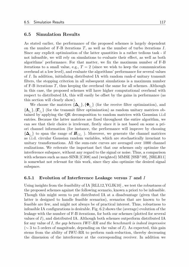
6.5. Simulation Results 117
6.5 Simulation Results
As stated earlier, the performance of the proposed schemes is largely dependenton the number of F-B iterations T , as well as the number of turbo iterations I.Since any explicit optimization of the latter quantities is a rather tedious task - ifnot infeasible, we will rely on simulations to evaluate their effect, as well as bothalgorithms’ performance. For that matter, we fix the maximum number of F-Biterations to a small value, e.g., T = 2 (since we wish to keep the communicationoverhead at a low level), and evaluate the algorithms’ performance for several valuesof I. In addition, initializing distributed IA with random rank-d unitary transmitfilters, the stopping criterion in all subsequent simulations is a maximum numberof F-B iterations T , thus keeping the overhead the same for all schemes. Althoughin this case, the proposed schemes will have higher computational overhead withrespect to distributed IA, this will easily be offset by the gains in performance (asthis section will clearly show).
We choose the matrices ∆∆∆lj, ΦΦΦlj (for the receive filter optimization), and
ΛΛΛlj, ΓΓΓlj (for the transmit filter optimization) as random unitary matrices ob-tained by applying the QR decomposition to random matrices with Gaussian i.i.dentries. Because the latter matrices are fixed throughout the entire algorithm, wecan see that their choice is irrelevant, firstly since it is not based on some a pri-ori channel information (for instance, the performance will improve by choosing∆∆∆lj
to span the range of HHH l,lj ). Moreover, we generate the channel matricesas i.i.d. circular Gaussian random variables, which are stochastically invariant tounitary transformations. All the sum-rate curves are averaged over 1000 channelrealizations. We reiterate the important fact that our schemes only optimize theinterference subspace, without any regard to the signal or noise. Thus, a comparisonwith schemes such as max-SINR [CJ08] and (weighted) MMSE [SSB+09], [SRLH11]is somewhat not relevant for this work, since they also optimize the desired signalsubspace.
6.5.1 Evolution of Interference Leakage versus T and I
Using insights from the feasibility of IA [RLL12,YGJK10] , we test the robustness ofthe proposed schemes against the following scenario, known a priori to be infeasible.Though this might seem to put distributed IA at a disadvantage (given that thelatter is designed to handle feasible scenarios), scenarios that are known to befeasible are few, and might not always be of practical interest. Thus, robustness toinfeasible IA configurations is desirable. Fig. 6.2 shows the (average) evolution of theleakage with the number of F-B iterations, for both our schemes (plotted for severalvalues of I), and distributed IA. Although both schemes outperform distributed IAfor any value of I, the gap between IWU-RR and the benchmark is indeed impressive(∼ 3 to 5 orders of magnitude, depending on the value of I). As expected, this gainstems from the ability of IWU-RR to perform rank-reduction, thereby decreasingthe dimension of the interference at the corresponding receiver. In addition we

118 Leakage Minimization Algorithms
1 2 3 4 5 6 7 8 9 1010
−4
10−3
10−2
10−1
100
101
F−B iteration (T)
Inte
rfere
nce L
eakage
IWU−RR
IWU−RP
Distributed IA
I=1 I=2,I=4
I=1
I=4
I=2
Figure 6.2: Interference Leakage as a function of T , I (4× 4 MIMO, 4 users, d = 2)
observe that the gain from each additional turbo iteration is decreasing: this isclearly visible in the case of IWU-RP, where the curves corresponding to I = 2 andI = 4 are almost identical, implying that only a few turbo iteration are needed togive the desired performance boost.
6.5.2 Sum-Rate Performance
Next, we simulate the ergodic sum-rate of both our schemes for a 10× 10 MIMO,4-user MIMO IC with d = 4, known to be proper [RLL12], and fix the number of F-B iterations to 2, for all algorithms. We use the distributed IA algorithm in [CJ08]as a benchmark, but most importantly, we also include the rank-one solution to(6.1.5), given by SDR. Fig. 6.3 reflects the effect of the turbo iteration on thesum-rate performance of both algorithms: by running just a few turbo iterations,we see that both schemes significantly outperform distributed IA, especially in thehigh SNR region, when the gain becomes very large! In addition we observe thatindeed the rank-one solution of SDR offers extremely poor performance in termsof sum-rate (as discussed in Sect. II.B). Moreover, we observe that the high-SNRslope for IWU-RR (I = 10) is higher than that of SDR, implying that on average,IWU-RR yields transmit / receive filters whose rank is larger than 1.
Moreover, we observe from Fig. 6.3 that the performance gap is very pronounced,e.g., the high-SNR spectral efficiency of IWU-RR with 10 turbo iterations is almost

6.5. Simulation Results 119
0 10 20 30 40 500
20
40
60
80
100
120
SNR(dB)
Erg
odic
Sum
−ra
te (
bp
s/H
z)
Distributed IA
IWU − RR (I = 1 )
IWU − RP (I = 1 )
IWU − RP (I = 10 )
IWU − RR (I = 10 )
SDR
Figure 6.3: Sum-rate of proposed schemes for 10 × 10 MIMO IC, 4 users (d = 4,T = 2), for different number of turbo iterations
0 10 20 30 40 500
5
10
15
20
25
30
35
40
SNR(dB)
Erg
odic
Sum
−ra
te (
bps/
Hz)
Distributed IA
IWU−RP (T = 2, I = 2 )
IWU−RR (T = 2, I = 2)
T=2
T=3
T=100
T=4
Figure 6.4: Sum-rate of proposed schemes for a 4 × 4 MIMO IC, 3 users (d = 2,T = 2), v/s distributed IA for different number of F-B iterations
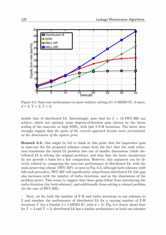
120 Leakage Minimization Algorithms
0 5 10 15 20 25 30 350
5
10
15
20
25
30
35
40
45
50
SNR(dB)
Erg
odic
Sum
−ra
te (
bp
s/H
z)
Distributed IA
SDR
IWU−RP
IWU−RR
Figure 6.5: Sum-rate performance in more realistic setting (8×8 MIMO IC, 4-users,d = 4, T = 2, I = 4)
double that of distributed IA. Interestingly, note that for I = 10 IWU-RR canachieve, albeit not optimal, some degrees-of-freedom gain (shown by the linearscaling of the sum-rate at high SNR), with just 2 F-B iterations. The latter doesstrongly suggest that the gains of the current approach become more accentuated,as the dimensions of the system grow.
Remark 6.3. One might be led to think at this point that the impressive gainin sum-rate for the proposed schemes comes from the fact that the rank reduc-tion transforms the initial IA problem into one of smaller dimensions (while dis-tributed IA is solving the original problem), and thus that the latter simulationsdo not provide a basis for a fair comparison. However, this argument can be di-rectly refuted by comparing the sum-rate performance of distributed IA, with therank-preserving scheme (IWU-RP): as seen in Fig. 6.3, although both schemes yieldfull-rank precoders, IWU-RP still significantly outperforms distributed IA (the gapalso increases with the number of turbo iterations, and as the dimensions of theproblem grow). This seems to suggest that those gains follow from introducing theturbo iteration (for both schemes), and additionally from solving a relaxed problem(in the case of IWU-RR).
Next, we fix both the number of F-B and turbo iterations in our schemes to2 and simulate the performance of distributed IA for a varying number of F-Biterations T (for a feasible 4× 4 MIMO IC, with d = 2). Fig. 6.4 clearly shows thatfor T = 2 and T = 3, distributed IA has a similar performance as both our schemes

6.5. Simulation Results 121
in the medium-to-low SNR region (and a worse one in the high-SNR region). It isonly for T = 4 that it starts to outperform them in the medium-to-low SNR regiononly. This implies that the overhead requirement of distributed IA is at least 50%more than our schemes, for this particular case (further simulations suggest thatthis trend increases with the system dimensions). Moreover, we see that distributedIA delivers its “optimal” performance after a large enough number of F-B are run(corresponding to extremely high communication overhead): this suggests that thepoor performance of dist IA in all simulations is due to the fact that there issignificant interference leakage for small values of T .
6.5.3 Performance in more realistic setupIn view of having a more realistic assessment - albeit still far from accurate - of thealgorithms’ performance, in somewhat more practical environments, we simulate8 × 8 MIMO transmission with 4 cells, 1 user per cell, 4 streams per user (fixingT = 2 for all algorithms, and I = 4 for our algorithms). We modify the gain of allinterfering channels (both intra and inter), such that the resulting SIR is −5dB,to (coarsely) emulate cell edge users. We can see from Fig. 6.5 that though bothschemes have a similar performance as distributed IA in the very low-SNR region,they outperform it for SNR values greater than 7dB (the gap being increasingwith the SNR): IWU-RR outperforms distributed IA by ∼ 30% at 15dB of SNR,and ∼ 80% at 20dB. This indeed shows that our schemes are good candidatesfor operating in such practical scenarios. On another note, we also see that IWU-RR and SDR have a similar high-SNR slope (thus implying that IWU-RR finds arank-one solution in almost all cases). However, the massive gap between IWU-RRand SDR, indicates that the solution provided by the IWU-RR yields significantlyhigher effective channel gain than the solution found by the SDR.
6.5.4 DiscussionsIt is interesting to notice in Fig. 6.3-6.5 that the gains for both schemes seem tohappen in the medium-to-high SNR region: this is expected, since in that regime,reducing interference is vital to increasing the sum-rate. The observed performanceboosts for both IWU-RR and IWU-RP are attributed to the introduction of theturbo-iteration. Furthermore, in the case of IWU-RR, the massive performance gainadditionally comes from the fact it is solving a relaxed problem. On another note,Fig. 6.3 shows that indeed the optimal rank-one solution to (6.1.5) provided bySDR is massively suboptimal in terms of sum-rate performance. This also providesa clear motivation for our work, where the proposed algorithms were mainly aimedat avoiding this rank-one solution.
Though negligible, one can indeed see a degradation in performance of bothschemes, with respect to distributed IA, in the low-SNR region (as seen fromFig. 6.3-6.6). Despite the that fact that full-rank filters are known to be optimal inthe high-SNR regime (thanks to the insights from interference alignment), in the

122 Leakage Minimization Algorithms
Figure 6.6: Ergodic sum-rate of proposed schemes vs distributed IA, as a functionof operating SNR (4× 4, 3-user MIMO IC d = 2, T = 2)
very low-SNR (interference-free) regime however, matched filtering is the optimalstrategy, and consequently rank-one filters are optimal as well. We note that al-though our rank-reducing algorithm does find a rank-one solution, it might be the“wrong one”, i.e., different from the matched filtering direction: this is due to thefact that both our algorithm and distributed IA look for solutions that reduce in-terference, that most likely are not aligned with the matched filtering direction. Onthe other hand, the full-rank solution given by distributed IA is likely to transmita reasonable amount of energy along that direction. This might explain the reasonthat distributed IA exhibits better performance than IWU-RR, in the low-SNRregion. Moreover, recall that schemes such as the proposed ones and distributedIA do not take into account the desired signal and noise subspace. As a result, onecan at best speculate about their low SNR behavior (since the SNR is not part oftheir mathematical formulation). However, referring to Fig. 6.6, we can see thatthis degradation is minimal (around 5% for IWU-RP and 8% for IWU-RR, overthe benchmark scheme). A possible alternative to mitigate this issue is to select thescheme based on the operating SNR, i.e., select IWU-RP in the low-SNR region,since it has a similar performance as distributed IA (as seen from Fig. 6.3-6.6): thiscan be easily implemented since both algorithms have the exact same structure,and only the updates have to be changed.
In conclusion, though both schemes are extremely similar in their algorithmicstructure (i.e. both update the filter weights within a turbo iteration), both aredistributed, optimize the same metric, and require the same (local) CSI quantities

6.6. Conclusion 123
at each node, they indeed have some fundamental differences. The fact that thefilter update equations are different has several implications: the update IWU-RRdoes not necessarily lead to full rank filters, and though it was shown that IWU-RR attempts to solve the relaxed problem in (4), such claim cannot be made forIWU-RP mainly due to the different constraints on the update structure. Finally,we compared their performance in several scenarios via simulations, and suggestedreasons for the behavior we observed.
6.6 Conclusion
Within the context of the leakage minimization problem, we proposed two distinctschemes based on rank-reducing (IWU-RR) and rank-preserving (IWU-RP) filterupdates, where the transmit and receive filter weights are iteratively refined in aturbo-like structure. We then showed that they are well suited for delivering highspectral efficiency (compared to the well-known distributed IA algorithm), whilegenerating very small overhead (typically, only a few F-B iterations). Though theintroduction of the so-called turbo iteration significantly boosted the performance ofboth schemes, it is clear that its impact was much more significant when combinedwith the rank-reducing updates in IWU-RR, thus allowing it to achieve a per-formance that otherwise required a much larger number of F-B iterations. In thatsense, the proposed schemes enabled us to tradeoff the communication overhead as-sociated with the F-B iterations - a rather expensive resource, with computationalcomplexity (an immensely cheaper resource).
6.7 Appendix
6.7.1 Proof of Proposition 6.2.1Given UUU and QQQ, and using the fact that QQQ and QQQ⊥ are unitary and orthogonal,the proof is simple after noting that any subspace UUU can be expressed as a sum ofits components over orthogonal directions (a result that trivially follows from theorthogonal decomposition theorem), i.e. UUU = PUPUPU +PPP⊥UUU , where PPP and PPP⊥ are anytwo orthogonal projection matrices. In particular, let PPP = QQQQQQ† and PPP⊥ = QQQ⊥QQQ⊥
† ,then UUU = QQQQQQ†UUU +QQQ⊥QQQ⊥
†UUU = QAQAQA+QQQ⊥BBB, where AAA = QQQ†UUU and BBB = QQQ⊥
†UUU
6.7.2 Proof of Lemma 6.2.1The result is a special case of [BE06], which shows that strong duality holds forall complex valued quadratic problems with up to two quadratic inequality con-straints. It is straightforward to show that (6.2.4) and its dual are strictly feasible.Furthermore, since the equality constraint ‖XXX‖2F = ζ is equivalent to the two in-equality constraints ‖XXX‖2F ≤ ζ and ‖XXX‖2F ≥ ζ, the results of [BE06] show that theglobally optimum solution of (6.2.4) can be obtained from its dual. For the specific
124 Leakage Minimization Algorithms
formulation (6.2.4), the solution takes a particularly simple form. Adding the La-grange multipliers of the two inequality constraints into a single dual variable µ,the necessary and sufficient conditions of [BE06, Theorem 2.4] can be written as(
γ22 TTT†QQQTTT + µ?III
)XXX? = −γ1γ2 TTT
†QQQΘΘΘ (6.7.1)
‖XXX‖2F = ζ (6.7.2)(γ2
2 TTT†QQQTTT + µ?III
) 0 . (6.7.3)
The last inequality is fulfilled when µ > −γ22 λ1[TTT †QQQTTT ] (µ = −γ2
2 λ1[TTT †QQQTTT ] canbe excluded since it results in ‖XXX‖2F =∞). Next, we study g(µ) 4= ‖XXX?(µ)‖2F − ζ.Let σ1, ..., σd be the eigenvalues of TTT †QQQTTT (sorted in increasing order), and vvv1, ..., vvvdtheir corresponding eigenvectors. We first rewrite g(µ) as
g(µ) = γ21γ
22 tr[ ΘΘΘ†QQQTTT (γ2
2 TTT†QQQTTT + µIII)−2TTT †QQQΘΘΘ ]− ζ
= γ21γ
22 tr[XXX†o( γ2
2 TTT†QQQTTT + µIII )−2XXXo]− ζ ,
where XXXo = TTT †QQQΘΘΘ. Note that we can express the matrix (γ22 TTT †QQQTTT + µIII)−2 as
a function of σi, vvvi, µ, as (γ22 TTT †QQQTTT + µIII)−2 =
∑di=1(γ2
2σi + µ)−2vvvivvv†i . Thus, we
rewrite g(µ) as follows,
g(µ) = γ21γ
22 tr[XXX†o(
d∑i=1
(γ22σi + µ)−2vvvivvv
†i )XXXo]− ζ
=d∑i=1
γ21γ
22 tr(XXX†ovvvivvv
†iXXXo)
(γ22σi + µ)2 − ζ =
d∑i=1
(γ1γ2 ci)2
(γ22σi + µ)2 − ζ, (6.7.4)
where ci = ‖XXX†ovvvi‖2. A quick look at this last expression reveals that indeed g(µ)is strictly monotonically decreasing in µ, for µ > −γ2
2σ1 = −γ22λ1[TTT †QQQTTT ]. Conse-
quently, g(µ) = 0 has a unique solution. To find the upper bound on µ to use in abisection search, note that if µ > 0 then
g(µ) < γ21γ
22
d∑i=1
‖XXX†ovvvi‖2
µ2 − ζ = γ21γ
22
µ2 ‖XXX†oVVV o‖2F − ζ =
(γ1γ2‖XXX†o‖F
µ
)2
− ζ .
where VVV o =[vvv1 . . . vvvd
]. Consequently if µ ≥ γ1γ2‖XXX†o‖F /
√ζ, we get g(µ) < 0.
This concludes the proof.
6.7.3 Proof of Lemma 6.3.1Let Sk be the set of local and global minima of (K2), which can written as,
Sk = x | p′(x) = 0, p′′(x) ≥ 0, 0 ≤ x < 1,

6.7. Appendix 125
where p(x) = (1− x2)e1 + x√
1− x2e2 + x2e3. We will show that the above set hasa single element, thereby establishing that (K2) is a convex problem, and derivethe solution.Defining a = e1 − e3, we start by finding the zero-differential points of p(x), i.e.,p′(x) = 0 ⇒ e2
1−2x2√
1−x2 = 2ax ⇒ 4(a2 + e22)x4 − 4(a2 + e2
2)x2 + e22 = 0 (e.1) where
the last equation stems from squaring both sides. Note that some of the roots of(e.1) will not correspond to zero-differential points (we will remedy this fact later).Letting X = x2, we can write the solution of (e.1) as,
X1 = 1/2 + a/2√a2 + e2
2, X2 = 1/2− a/2√a2 + e2
2.
Moreover, since we are interested in solutions to (K2) that lie in the interval [0, 1],we verify that indeed X1, X2 lie in this interval. This can be easily done by con-sidering two cases, a ≥ 0 and a ≤ 0. Using exactly the same manner, we can showthat if a ≤ 0, then 0 ≤ X1 ≤ 1/2 and 1/2 ≤ X2 ≤ 1, thus concluding that bothlie in the interval [0, 1]. This said, by discarding negative solutions, the solution to(e.1) is x1 =
√X1, x2 =
√X2, i.e.,
x1 =√X1 =
√1/2 + a/2
√a2 + e2
2,
x2 =√X2 =
√1/2− a/2
√a2 + e2
2.
Note that both x1 and x2, lie in the interval [0, 1]. Recall that not all the solutionsof (e.1) correspond to zero-differential points of p(x) - in fact it is easy to show thatp′(x1) = 0 and p′(x2) 6= 0, implying that p(x) has a single unique zero-differentialpoint at x1. Thus, it remains to show that p′′(x1) = 0. Using the fact that x2
1 = X1,x2
2 = X2, and noting that X1 +X2 = 1, we rewrite this condition as,
p′′(x1) ≥ 0⇔ −2a− e2
[(X1X2
)3/2+ 3
(X1X2
)1/2]≥ 0
The last equation can be easily shown, by plugging in the values for X1 and X2(we will omit the derivations since they are rather straightforward and easily re-produced).
Thus, we conclude that the set of global minima of p(x), Sk, has a single element,thereby establishing that p(x) is convex and has single global minimum given bySk =
√1/2 + a/2
√a2 + e2
2.


Part III
Cloud Radio Access Networks
127


Chapter 7
Antenna Domain Formation
7.1 Densification
In the context of cellular systems (and this thesis in particular), densification,refers to having more BSs per unit area, and more antennas per BS. More-over, ultra-dense deployments have been identified as one of the key scenarios
for 5G systems [MET14]. From a historical perspective, densification has giventhe most significant gains in data rates. This is due to the fact that, in general,more BSs / antennas, lead to more degrees-of-freedom. This is of course contingentupon having effective ways of dealing with the resulting interference (since den-sification results in more interference). Indeed, the fundamental insights providedby techniques such as Interference Alignment [CJ08,MAMK08], and CoordinatedMulti-point [GHH+10], clearly state that the effective managing of interference (viacoordination among BSs) is necessary to achieve the optimal degrees-of-freedom, inseveral communication scenarios.
While we have motivated and investigated mechanisms for distributed coordi-nation in Part II (focusing on ones with low-overhead), we attempt to shed lighton the opposing paradigm of centralized coordination. Intuitively speaking, tightercoordination can be achieved, when BSs stations are connected via high-capacitylinks to a so-called aggregation node, that can be used to share CSI and/or dataamong the different BSs. This is the basic setup of the so-called Cloud Radio AccessNetwork (Could-RAN).
Typically, a Cloud-RAN consists of Remote Radio Heads (RRHs) (assumedto have limited baseband/processing capabilities) which are connected to the so-called Aggregation Nodes (ANs) (assumed to have perfect and global CSI), viawired/wireless links. In that sense, aggregation nodes act as centralized computenodes, that gather all the required CSI from a cluster of connected radio-heads,perform the required optimization (e.g., precoding), and send the resulting param-eters to the relevant radio-heads. An Antenna Domain (AD) is the collection ofradio-heads connected to a particular aggregation node. It is envisioned that eachantenna domain consists of a few (up to tens of) radio-heads, and serves a few dozen(up to a hundred) users. The investigation of such setups, i.e., where base stations
129

130 Antenna Domain Formation
are connected via backhauls, was originally done in [ZQL13].So far, all such approaches assume the presence of one antenna domain / aggre-
gation node: The problem reduces to managing intra-AD interference only, assum-ing no inter-AD interference is present. The authors in [LHMJL13] investigateddynamic clustering of base stations, where users within each cluster are served ina Joint Transmission (JT)-like manner. The same model was adopted in [ZTCY15]and [TCZY15], where the authors consider the problem of forming BS clusters inthe presence of caching and multi-cast transmission. A similar model for coordi-nation was employed in [DY16], focusing on energy efficient transmission instead.In [RGIG15], (looser) coordination among the radio-heads within the antenna do-main was investigated (where Coordinated Beamforming (CB)-type precoding wasemployed). Obviously, the model adopted by all such approaches - where all thenetwork is coordinated by one aggregation node, is not scalable.
10
System-wide Operation
AD 1
AN 1
AN 2
AD 2
VVV 1
VVV 2
VVV 3
VVV 4
VVV 5
Figure 7.1: Toy Example: intra-AD vs inter-AD interference (VVV 1, ...,VVV 5 are pre-coders at the RRHs)
Going to the multi-AD/multi-AN setting, although the management of bothinter-AD and intra-AD interference (Fig. 7.1) becomes a critical problem, it remainsunaddressed yet. This is what we refer to as the Antenna Domain Formation (ADF)problem:
(A) Given a set of radio-heads, each serving a set of users (Fig. 7.2), what is theoptimal assignment of radio-heads to aggregation nodes, that minimizes theinter-AD interference?
(B) Given an initial state (i.e., assignment of users to radio-heads, and radio-heads
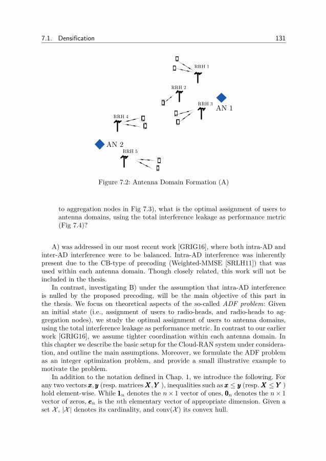
7.1. Densification 131
RRH 2
RRH 3
RRH 4
RRH 1
AN 1
AN 2RRH 5
Figure 7.2: Antenna Domain Formation (A)
to aggregation nodes in Fig 7.3), what is the optimal assignment of users toantenna domains, using the total interference leakage as performance metric(Fig 7.4)?
A) was addressed in our most recent work [GRIG16], where both intra-AD andinter-AD interference were to be balanced. Intra-AD interference was inherentlypresent due to the CB-type of precoding (Weighted-MMSE [SRLH11]) that wasused within each antenna domain. Though closely related, this work will not beincluded in the thesis.
In contrast, investigating B) under the assumption that intra-AD interferenceis nulled by the proposed precoding, will be the main objective of this part inthe thesis. We focus on theoretical aspects of the so-called ADF problem: Givenan initial state (i.e., assignment of users to radio-heads, and radio-heads to ag-gregation nodes), we study the optimal assignment of users to antenna domains,using the total interference leakage as performance metric. In contrast to our earlierwork [GRIG16], we assume tighter coordination within each antenna domain. Inthis chapter we describe the basic setup for the Cloud-RAN system under considera-tion, and outline the main assumptions. Moreover, we formulate the ADF problemas an integer optimization problem, and provide a small illustrative example tomotivate the problem.
In addition to the notation defined in Chap. 1, we introduce the following. Forany two vectors xxx,yyy (resp. matricesXXX,YYY ), inequalities such as xxx ≤ yyy (resp.XXX ≤ YYY )hold element-wise. While 111n denotes the n× 1 vector of ones, 000n denotes the n× 1vector of zeros, eeen is the nth elementary vector of appropriate dimension. Given aset X , |X | denotes its cardinality, and conv(X ) its convex hull.
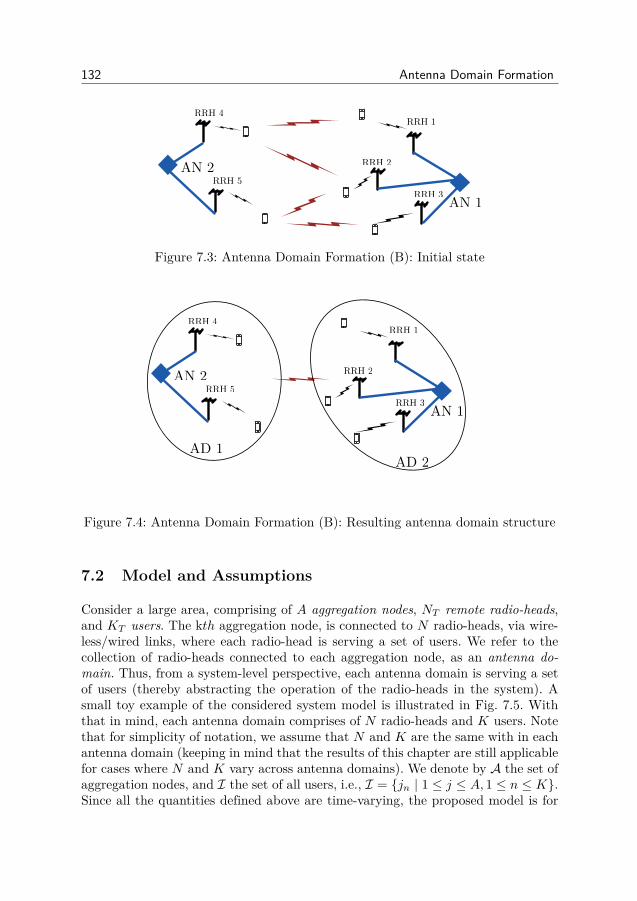
132 Antenna Domain Formation
RRH 2
RRH 3
RRH 4RRH 1
AN 1
AN 2RRH 5
Figure 7.3: Antenna Domain Formation (B): Initial state
RRH 2
RRH 3
RRH 4RRH 1
AN 1
AN 2RRH 5
AD 1AD 2
Figure 7.4: Antenna Domain Formation (B): Resulting antenna domain structure
7.2 Model and Assumptions
Consider a large area, comprising of A aggregation nodes, NT remote radio-heads,and KT users. The kth aggregation node, is connected to N radio-heads, via wire-less/wired links, where each radio-head is serving a set of users. We refer to thecollection of radio-heads connected to each aggregation node, as an antenna do-main. Thus, from a system-level perspective, each antenna domain is serving a setof users (thereby abstracting the operation of the radio-heads in the system). Asmall toy example of the considered system model is illustrated in Fig. 7.5. Withthat in mind, each antenna domain comprises of N radio-heads and K users. Notethat for simplicity of notation, we assume that N and K are the same with in eachantenna domain (keeping in mind that the results of this chapter are still applicablefor cases where N and K vary across antenna domains). We denote by A the set ofaggregation nodes, and I the set of all users, i.e., I = jn | 1 ≤ j ≤ A, 1 ≤ n ≤ K.Since all the quantities defined above are time-varying, the proposed model is for

7.2. Model and Assumptions 133
each scheduling time-slot (thus, any time-related indexes are omitted).Radio-heads are assumed to have limited baseband/processing capabilities, re-
stricted to precoding only. Moreover, aggregation nodes act as “large” centralizedprocessors, that gather channel state information (CSI) from all the users, performthe required processing/optimization, and communicate the optimal precoders tothe radio-heads. To avoid complicating the notation, we assume that each radiohead is equipped with M antennas, while each user has a single antenna. This canbe extended to multiple antennas at the receiver, and different antenna configura-tion in a straightforward manner
We outline the main assumptions used throughout this part of the thesis.
Assumption 7.2.1 (Synchronization). The different radio-heads within each ADare tightly synchronized, e.g., phase-level synchronization, essentially acting as alarge virtual antenna array. Each antenna domain consists of a small number ofRRHs (typically 2 ∼ 4).
Assumption 7.2.2 (CSI). Global and perfect CSI is assumed to be a priori avail-able at each of the aggregation nodes.
Assumption 7.2.3 (Zero intra-AD interference). The precoding within each an-tenna domain, is designed in such a way that no intra-antenna domain interferenceis present, i.e., no interference among users within the same antenna domain.
We underline at this point that such assumptions are quite common for Cloud-RAN related performance studies (e.g., [ZTCY15, TCZY15, LHMJL13]). Thoughthe resulting systems tend to have large overhead and complexity, we reiterate thatthe main aim of this work is the study of performance bounds for antenna domainsystems, rather than practical design paradigms. More light is shed on the overheadin Sect. 8.4.3.
Let jn denote the index of the nth user, in the jth antenna domain, jn ∈ I.Then, its received signal is given by (assuming a downlink transmission scenario),
yjn =K∑q=1
hhhj,jnvvvjqsjq√pj +
A∑i 6=j
K∑m=1
hhhi,jnvvvimsim√pj + njn (7.2.1)
where hhhi,jn ∈ C1×MN is the (MISO) channel from antenna domain i to user jn,vvvim ∈ CMN×1 the beamforming vector to user im ∈ I, sim the data symbol for userim ∈ I such that E[sims
†im
] = 1, njn the AWGN noise for user jn ∈ I such thatE[njnn
†jn
] = σ2jn, and pj the transmit power for antenna domain j ∈ A. Moreover,
the proposed precoding design, i.e., zero intra-AD interference (Sect. 7.2), translatesto the following,
hhhj,jnvvvjq =βj , ∀n = q
0 , ∀n 6= q, ∀j ∈ A (7.2.2)

134 Antenna Domain Formation
where βj > 0 is a free parameter that is chosen to satisfy the maximum transmitpower constraint on the transmit precoder (per antenna domain), i.e.,
K∑q=1‖vvvjq‖22 ≤ K, ∀j ∈ A (7.2.3)
The resulting received signal and SINR are,
yjn = βjsjn√pj +
A∑i 6=j
K∑m=1
hhhi,jnvvvimsim√pi + njn
γjn =β2j pj∑A
i6=j∑Km=1 pi|hhhi,jnvvvim |2 + σ2
jn
(7.2.4)
where SNRjn = pjβ2j /σ
2jn
is the SNR of user jn. Assuming optimal encoding/decoding,and treating interference as noise, the achievable sum-rate of the network is givenby,
RΣ =A∑j=1
K∑n=1
log2(1 + γjn) (7.2.5)
7.2.1 MotivationWe denote by ψim,jn the so-called interference coupling coefficient between usersim and jn,
ψim,jn =pi|hhhi,jnvvvim |2, ∀ (im, jn) ∈ I2, im 6= jn,
0 , ∀im = jn
ψim,jn denotes the interference that user im ∈ I causes to user jn ∈ I. Moreover,we recall that ψim,jn 6= ψjn,im . Let ΨΨΨ ∈ RKT×KT+ be the matrix formed by gatheringall the coupling coefficients, i.e.,
[ΨΨΨ]jn,im =ψjn,im , ∀i 6= j
0,∀i = j,∀ (jn, im) ∈ I2, (7.2.6)
and
xk,jn ∈ 0, 1, ∀ jn ∈ I, k ∈ A (7.2.7)
be the assignment variable for user jn to antenna domain k. With that in mind,gjn , the total interference leakage seen by user jn ∈ I, is given by,
gjn(xk,jn) ,∑k∈A
∑l∈Al 6=k
∑im∈Iim 6=jn
xk,imψim,jnxl,jn
(7.2.8)

7.3. Problem Formulation 135
where xk,jn denotes the set of all assignment variables. The total interferenceleakage, f , is then
f(xk,jn) ,∑jn∈I
gjn(xk,im) (7.2.9)
and can be rewritten as,
f(xk,jn) ,∑k∈A
∑l∈Al 6=k
∑jn∈I
∑im∈Iim 6=jn
xk,imψim,jnxl,jn
(7.2.10)
Recall that due to the proposed precoding (i.e., zero intra-AD interference), theinter-AD interference leakage coincides with the total interference leakage, f , in thesystem.
Example 7.2.1 (Motivating Example). Consider the following toy example withA = 2, K = 2, N = 1 (Fig. 7.5). Then the cost in (7.2.10) reduces to,
f(xk,jn) =∑im∈I
∑jn 6=im
x1,imψim,jnx2,jn , I = 11, · · · , 22
Now the intuition behind the above cost becomes clear: the cost of having users imand jn in different antenna domains is ψim,jn + ψjn,im , and zero otherwise. Thatsame criterion is the reason that intra-AD interference is not accounted for, in f .The last equation shows that the total interference leakage in this network (Fig. 7.5)corresponds to setting all the assignment variables to one, i.e., f(xk,jn = 1) - a“naive” assignment. Thus, better performance can be reaped-off with a “smarter”assignment. This is the main motivation for using a cost function such as (7.2.10).
7.3 Problem Formulation
In the last part, we motivated the effect of assigning users to antenna domains.That is the so-called ADF problem, that is formalized below.
Definition 7.3.1 (Antenna Domain Formation (ADF)). Given an initial state(i.e., assignment of users to radio-heads, and radio-heads to aggregation nodes),the ADF problem is given by the optimal assignment of users to antenna domains,w.r.t. minimizing the total interference leakage in the system. The correspondingoptimization problem is the integer programming problem shown below,
(P )
minxk,jn
f =∑Ak=1
∑Al 6=k(
∑jn
∑im 6=jn xk,imψim,jnxl,jn)
s. t.∑imxk,im = ρk, ∀k ∈ A∑A
k=1 xk,im ≤ 1, ∀im ∈ Ixk,im ∈ 0, 1, ∀(k, im) ∈ A× I
(7.3.1)

136 Antenna Domain Formation
AN
RRH
user 11
user 12
user 21
user 22
11,21 + 21,11
12,22 + 22,12
11 ,2
2+ 22 ,1
1
12,21
+ 21
,12
AN
RRH
Figure 7.5: Toy Example (interference marked in red): total interference equal tointer-AD interference
The first constraint specifies that ρk ∈ Z+ users are to be assigned to eachantenna domain, i.e., the loading constraint. Such a constraint is needed for the sakeof load balancing on the backhaul (i.e., to prevent highly asymmetric cases whereall users get assigned to one antenna domain, while the rest are idle). Moreover, thesecond constraint, i.e., the assignment constraint, ensures that each user is assignedto at most one antenna domain. As a result, when
∑k∈A < KT , some users are
not assigned to any antenna domain. Another way to interpret (P ) is from a userassignment/selection perspective: given an initial state with K users (where Klarge), the goal is to select the optimal subset (of size ρk < K), that minimizes theinterference leakage.
We first start by rewriting (P ) in vector and matrix form - both of which willbe used later in the text (keeping in mind that all are equivalent). Let xxxk be theaggregate assignment vector for antenna domain k to all other users, and XXX theaggregate assignment matrix for the system,
xxxk = [xk,11 , · · · , xk,AK ]T , xxxk ∈ BKT ,∀k ∈ AXXX = [xxx1, ....,xxxA] ∈ BKT×A
Proposition 7.3.1. (P ) can be rewritten in equivalent vector form,
(P )
min f(xxxk) =
∑Ak=1
∑Al 6=k xxx
TkΨΨΨxxxl
s. t.∑Ak=1 xxxk ≤ 111KT ,
111TKTxxxk = ρk, xxxk ∈ BKT , ∀k ∈ A(7.3.2)
and matrix form
(P )
min f(XXX) = tr(XXXTΨΨΨXXXΩΩΩ)s. t. XXX111A ≤ 111KT , XXX ∈ Sρ
(7.3.3)

7.3. Problem Formulation 137
where we denote by Sρ the set of all KT ×A binary matrices, that satisfy the loadingconstraint, i.e.,
Sρ , QQQ ∈ BKT×A | QQQT111KT = ρρρ (7.3.4)
ρρρ , [ρ1, ..., ρA]T , and ΩΩΩ , 111A111TA − IIIA.
Proof. The derivations are shown in Appendix 8.7.1.
It can be seen from (7.3.2) that f is not jointly convex in all the variables,due to the coupling among them. However, we underline the inherent multi-linearnature of f (taken separately in each variable, f is linear), that we exploit for theoptimization.

Chapter 8
Proposed Approach
In the previous chapter, we motivated and formulated the ADF problem, (P )in (7.3.1), as an integer optimization problem. In this chapter, we then employBlock-Coordinate Descent (BCD) - that we have earlier developed in [GRIG16],
to iteratively solve the problem. The lack of theoretical guarantees on the obtainedsolution, as well as the complicated nature of the problem, motivates us to find use-ful and meaningful lower bounds on the ADF problem (since it represents the totalinterference leakage). For that purpose, we derive the corresponding Dantzig-Wolfe(DW) decomposition (a Linear Program (LP) with exponentially many variables),and adapt the Column Generate Method (CGM) to compute the DW lower bound.We also derive the dual problem (a natural lower bound), characterize the dual-ity gap, and show that the DW lower bound is tighter than of the dual problem(and consequently all related methods such as dual subgradient ascent, and La-grange relaxation). Finally, we provide some numerical results that highlight theperformance of our proposed algorithm.
8.1 Algorithm
Our proposed approach consists of two parts, where the first one concerns theoptimal assignment of users to antenna domains, i.e., obtaining a solution to the socalled ADF problem in (7.3.1). Parts of the approach ware presented in our earlierwork [GRIG16] - albeit for a different system model. They are still summarizedhere for completeness. In the second part, we develop the precoding mechanism.We first present the following definition.
Definition 8.1.1 (Integrality Property for Linear Programming). Consider thefollowing binary linear program (LP),
(P ) xxx? = minxxx
cccTxxx, s. t. xxx ∈ C, xxx ∈ BN ,
and its continuous relaxation (CR) (also known as LP relaxation),
(CR) xxx = minxxx
cccTxxx, s. t. xxx ∈ C, 000N ≤ xxx ≤ 111N ,
139
140 Proposed Approach
where C is a convex set. The set C is said to satisfy the integrality property if all itsvertexes correspond to integers: it is well-known for such cases, that the so-calledcontinuous relaxation (CR) is optimal [Fra05], and consequently, xxx is integer aswell, and xxx = xxx.
8.1.1 Algorithm Description
Due to the coupled nature of the objective function in (7.3.2), we leverage thewell known Block-Coordinate Descent (BCD) method, that has been applied toseveral areas of signal processing, namely, transmitter and receiver optimization incellular networks [SRLH11, SSB+09,GKBS15,GCJ11]. In what follows, n denotesthe iteration number, i.e., xxx(n)
k denotes the value of xxxk at the nth iteration. Wedenote by zzz(n)
k = xxx(n+1)1 , ...,xxx
(n+1)k−1 ,xxx
(n)k+1, ...,xxx
(n)A the block of fixed variables, for
the kth update at the nth iteration.Our exposition here will be summarized, since the full details of the algorithm
are shown in [GRIG16]. All the derivations/formulations of this part are based on(P ), as shown in (7.3.2). We let f(xxxk, zzz(n)
k ) denote the function f(xxxk), when thevariables in block zzz(n)
k are fixed, which can be written as,
f(xxxk, zzz(n)k ) = xxxTkΨΨΨ
(k−1∑l=1
xxx(n+1)l +
A∑l=k+1
xxx(n)l
),
, xxxTk rrr(n)k , (8.1.1)
where rrr(n)k is referred to as the residual of antenna domain k, at the nth iteration.
Looking at the above equation, f(xxxk, zzz(n)k ) is linear in xxxk, implying that f is linear
in each block of variables. The application of BCD yields the following update forxxxk, at the nth iteration.
xxx(n+1)k =
argminxxxk
f(xxxk, zzz(n)k )
s. t. 111TKTxxxk = ρk, xxxk ≤ ωωωk, xxxk ∈ BKT ,(8.1.2)
where ωωωk , 111KT −∑l 6=k xxxl is the set of feasible assignments for xxxk. The above
problem belongs to the class of Mixed-Integer Linear Programs (MILPs). Moreover,it is a special case of the generalized assignment problem (GAP). Though the genericformulation of GAP is known to be NP-hard, we exploit the particular structureof (8.1.2), to show that it is equivalent to a LP. Let C be the set formed by thefirst two constraints in (8.1.2), i.e., C = 111TKTxxxk = ρk, xxxk ≤ ωωωk. Recalling thatρk and ωωωk are integers (by construction), one can see that the vertexes of C areintegers, and thus satisfies the integrality property (as presented in Definition 8.1.1).Thus, following the result of Definition 8.1.1, its continuous relaxation will yield

8.1. Algorithm 141
the optimal solution. Thus, the last problem is equivalent to,
xxx(n+1)k =
argminxxxk
f(xxxk, zzz(n)k )
s. t. 111TKTxxxk = ρk, xxxk ≤ ωωωk, 000KT ≤ xxxk.(8.1.3)
As seen from (8.1.1), when xxxll 6=k are fixed, the cost function decouples in xxxk’sand can thus be solved locally at antenna domain k, in a fully distributed manner :Each aggregation node solves its own subproblem - a linear program, without anyloss in optimality. The process is formalized in Algorithm 7. In a nutshell, theoptimal update for xxxk at antenna domain k, is a function of the assignments at allthe other antenna domains (that thus have to be shared): Given assignments fromother antenna domains, (xxx(n+1)
1 , ...,xxx(n+1)k−1 ,xxx
(n)k+1, ...,xxx
(n)A ), antenna domain k forms
the residual rrr(n)k , and can proceed to solve its optimization problem locally, and
update xxx(n+1)k .
Algorithm 7 ADF via BCDInput: ΨΨΨ, KT , ρρρ, Afor n = 0, 1, · · · , L− 1 do
// procedure at each aggregation nodeobtain (xxx(n+1)
1 , ...,xxx(n+1)k−1 ,xxx
(n)k+1, ...,xxx
(n)A ) at antenna domain k
compute residual rrr(n)k using (8.1.1)
compute feasible assignment ωωωk using (8.1.2)compute xxx(n+1)
k as solution to (8.1.3)end forOutput: XXX(L) = [xxx(L)
1 , ...,xxx(L)A ]
8.1.2 Convergence
Let xxx(n)k be the sequence iterates produced by the BCD in (8.1.3), and xxxok ,
limn→∞xxx(n)k . The monotonic nature of the BCD iterates was established in our
earlier work [GRIG16], and is presented below for completeness.
Lemma 8.1.1 (Monotonicity). With each update xxx(n)k → xxx
(n)k+1, f is non-increasing.
Moreover, the sequence of function iterates f(xxx(n)1 , ...,xxx
(n)A )n converges to a limit
point f(xxxok).
Proof. Refer to Appendix 8.7.4
Although the above result establishes the convergence of the proposed BCDmethod, it only establishes convergence to a limit. However, showing that thislimit is a stationary point of f is not possible under the BCD framework, due to

142 Proposed Approach
the coupled nature of the assignment constraint (7.3.2). Even the strongest BCDconvergence results such as [Tse01] cannot establish convergence to a stationarypoint.
8.1.3 PrecodingThis far, we have only focused on the specifics of the ADF problem, while ignoringthe precoding. The main idea behind the precoder design is to null all intra-ADinterference, as shown in (7.2.2) and (7.2.3). More intuition could be gained byrewriting the signal model (7.2.1) in vector form,
yyyj = HHHj,jVVV jsssj√pj +
A∑i6=j
HHHi,jVVV isssi√pi +nnnj , (8.1.4)
where yyyj is the vector of received signals for users served by antenna domain j. Inthe above,
HHHi,j ,
hhhi,j1
...hhhi,jK
,VVV i , [vvvi1 , · · · , vvviK ]and sssi ,
si1...siK
(8.1.5)
denote the channel between the antennas of antenna domain i and the users ofantenna domain j, the matrix of precoding vectors for antenna domain i, andthe vector of transmit symbols for users of antenna domain i, respectively. Then,zero intra-AD interference condition, i.e., (7.2.2) and the maximum transmit powerconstraint, i.e., (7.2.3) are equivalently written,
HHHi,iVVV i = βiIIIK , and ‖VVV i‖2F ≤ K , ∀i ∈ A (8.1.6)
Note that the total interference leakage f , can be equivalently written as,
f ,A∑i=1
A∑j 6=i‖HHHi,jVVV i‖2F =
A∑i=1
A∑j 6=i
tr(HHHi,jVVV iVVV†iHHH†i,j)
=A∑i=1
tr[VVV †i (A∑j 6=i
HHH†i,jHHHi,j)VVV i] ,A∑i=1
tr(VVV †iRRRiVVV i) , h(VVV i). (8.1.7)
Note that while f in (7.2.10) denotes the interference leakage expressed as a functionof the assignment variables, h denotes interference leakage expressed as function ofthe precoders. Though the two are equal, we make that distinction for clarity. Theprecoder optimization problem for antenna domain i, is then formulated as follows.
VVV ?i =
argminVVV i
h(VVV i) = tr(VVV †iRRRiVVV i)
s. t. HHHi,iVVV i = βiIIIK .(8.1.8)

8.2. Relaxations and Performance Bounds 143
Note that the transmit power constraint can be explicitly enforced, since it can besatisfied by changing the free parameter βi. The solution for this problem is a specialcase of the next result (by setting di = K), where the solution is parametrized asa function of some di, and solved for the general case.
Proposition 8.1.1. Consider the following convex problem.
VVV ?i =
argminVVV i∈CMN×di
tr(VVV †iRRRiVVV i)
s. t. HHHi,iVVV i = βiIIIdi , di ∈ Z++
(8.1.9)
where RRRi =∑Aj 6=iHHH
†i,jHHHi,j , HHHi,j ∈ Cdi×MN , βi is a free parameter chosen to satisfy
the transmit power constraint, ‖VVV i‖2F = di. The globally optimal solution is givenby
VVV ?i =
√di RRR
−1i HHH†i,i
(HHHi,iRRR
−1i HHH†i,i
)−1
‖RRR−1i HHH†i,i
(HHHi,iRRR
−1i HHH†i,i
)−1‖F
. (8.1.10)
Moreover, for di ≤MN , the problem is feasible almost surely.
Proof. Refer to Appendix 8.7.2
8.2 Relaxations and Performance Bounds
It should be clear at this stage that problems such as (P ) are quite challenging. Thisis further highlighted by the findings of the previous section: despite the widespreadeffectiveness of methods such as BCD, one is not able to show any stationarity ofthe obtained solution (i.e. no local optimality can be established). Moreover, it ishard to theoretically ascertain how ‘close’ is an obtained solution to optimality.To compensate for those shortcomings, finding meaningful lower bounds on (P )is of interest: that is particularly relevant for our case, since the cost function, f ,represents an actual physical quantity. Moreover, as discussed earlier in Sec. 7.2.1,finding lower bounds on the interference leakage f , result in finding upper bounds onthe sum-rate. For the problem at hand we derive the corresponding Dantzig-Wolfe(DW) decomposition, and establish that although the resulting problem is a LP, ithas exponentially many variables. We thus adapt the Column Generation Method(CGM), for our particular problem. We also derive the dual problem for (P ), andshow that it yields a looser lower bound on (P ). We thus conclude that methodsthat are based on the dual problem (e.g., Dual Subgradient Ascent, Lagrange Re-laxation), offer worse lower bounds, than ones based on the DW decomposition(e.g., CGM).
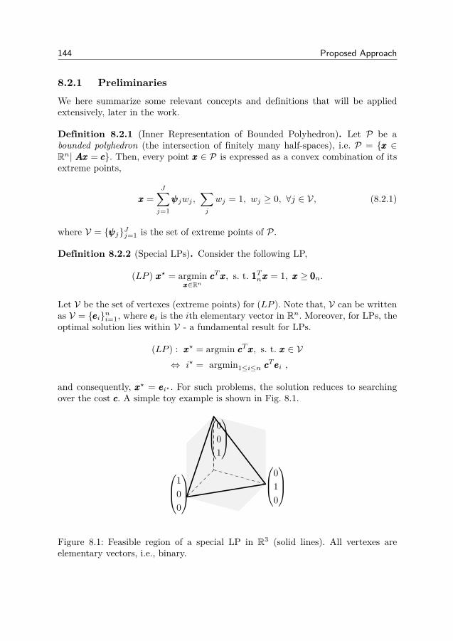
144 Proposed Approach
8.2.1 Preliminaries
We here summarize some relevant concepts and definitions that will be appliedextensively, later in the work.
Definition 8.2.1 (Inner Representation of Bounded Polyhedron). Let P be abounded polyhedron (the intersection of finitely many half-spaces), i.e. P = xxx ∈Rn| AAAxxx = ccc. Then, every point xxx ∈ P is expressed as a convex combination of itsextreme points,
xxx =J∑j=1
ψψψjwj ,∑j
wj = 1, wj ≥ 0, ∀j ∈ V, (8.2.1)
where V = ψψψjJj=1 is the set of extreme points of P.
Definition 8.2.2 (Special LPs). Consider the following LP,
(LP ) xxx? = argminxxx∈Rn
cccTxxx, s. t. 111Tnxxx = 1, xxx ≥ 000n.
Let V be the set of vertexes (extreme points) for (LP ). Note that, V can be writtenas V = eeeini=1, where eeei is the ith elementary vector in Rn. Moreover, for LPs, theoptimal solution lies within V - a fundamental result for LPs.
(LP ) : xxx? = argmin cccTxxx, s. t. xxx ∈ V⇔ i? = argmin1≤i≤n ccc
Teeei ,
and consequently, xxx? = eeei? . For such problems, the solution reduces to searchingover the cost ccc. A simple toy example is shown in Fig. 8.1.
100
0
10
001
Figure 8.1: Feasible region of a special LP in R3 (solid lines). All vertexes areelementary vectors, i.e., binary.

8.2. Relaxations and Performance Bounds 145
In what follows, we define the following notation,
Sρ , QQQjSj=1, S = |Sρ|
αj , tr(QQQTj ΨΨΨQQQjΩΩΩ), ∀j = 1, · · · , Sqqqj ,QQQj111A − 111KT , ∀QQQj ∈ Sρ, qqqj ∈ ZKT
ΓΓΓ , [qqq1, · · · , qqqS ], ΓΓΓ ∈ ZKT×S+ . (8.2.2)
Moreover, note that Sρ has a decomposable structure, i.e. Sρ ,W(ρ1)×· · ·×W(ρA)where W(ρi) = xxx ∈ BKT | 111TKTxxx = ρi. Thus,
S , |Sρ| =A∏i=1|W(ρi)| where |W(ρi)| =
(KT
ρi
). (8.2.3)
Remark 8.1. As it will become clear in this section, some of the decomposi-tions/relaxations in question are computationally demanding. However, we under-line the fact that such methods are intended for benchmarking purposes: they areintended to run during an offline training phase, where “enough” computationalresources are available. Thus, the computation of quantities such as ΨΨΨ,Sρ, αj , qqqjand ΓΓΓ is not a limiting factor.
8.2.2 Dantzig-Wolfe DecompositionInitially proposed in their seminal paper [GBD60b], the Dantzig-Wolfe decompo-sition has been widely adopted by the operations research community, for findingbounds on integer programming problems. Based on our above definitions in (8.2.2),we can rewrite Sρ and (P ) as,
Sρ = XXX =S∑j=1
wjQQQj |S∑j=1
wj = 1, wj ∈ B,∀j, (8.2.4)
(P )
min f(XXX) = tr(XXXTΨΨΨXXXΩΩΩ)s. t. XXX ∈ Sρ, XXX111A ≤ 111KT .
(8.2.5)
The above problem is still difficult to tackle, due to the combinatorial nature ofXXX ∈ Sρ . The DW decomposition then proceeds by relaxing XXX ∈ Sρ, into a convexone, by taking its convex hull, i.e.,
conv(Sρ) = XXX =S∑j=1
wjQQQj | 111TSwww = 1, 000S ≤ www. (8.2.6)

146 Proposed Approach
As a result, every point in conv(Sρ) is represented as a convex combination ofthe extreme points of conv(Sρ) (detailed in Definition 8.2.1). Since Sρ ⊆ conv(Sρ),the resulting problem (PDW ), is a lower bound on (P ),
(PDW )
min f(XXX) = tr(XXXTΨΨΨXXXΩΩΩ)s. t. XXX ∈ conv(Sρ), XXX111A ≤ 111KT .
(8.2.7)
Note that the assignment constraint can be written in an equivalent form,
XXX111A ≤ 111KT ⇔ (∑j
wjQQQj)111A ≤ 111KT ⇔ (∑j
wjQQQj111A) ≤ 111KT
⇔∑j
wjqqqj + (∑j
wj)111KT ≤ 111KT ⇔ ΓΓΓwww ≤ 000KT ,
where the last one follows from the fact that∑j wj = 1 (as defined by the DW
decomposition). Moreover, recalling that αj , tr(QQQTj ΨΨΨQQQjΩΩΩ), ∀j, and letting www =(w1, · · · , wS)T , (8.2.7) is equivalent to,
(PDW )
minwww
αααTwww
s. t. ΓΓΓwww ≤ 000KT , 111TSwww = 1, www ≥ 000S .(8.2.8)
A few remarks are in order at this stage. Note that despite the combinatorial andnon-convex nature of (P ), the DW always results in a linear program (providedthat Sρ is a bounded polyhedron). However, there is the additional caveat thatthough (8.2.8) is a LP, it has an exponential number of variables, S: it is unfit forconventional LP solvers. We thus adapt the Column Generate Method (CGM), forour particular problem.
Remark 8.2. We note that (8.2.6) clearly shows that the DW decomposition isa mapping from XXX in (7.3.3), to www in (8.2.8). However, this mapping is evidentlynot one-to-one, since XXX uniquely reconstructs from www, but not vice versa [LD05].
Solution via Column Generation Method
The Column Generation Method (CGM), attempts to iteratively solve (8.2.8),thereby mitigating the need for directly solving it: starting from ΓΓΓ0 - a matrixconsisting of a subset of mo columns of ΓΓΓ, one first solves the resulting restrictedmaster problem (RMP), i.e. a reduced version of (8.2.8). Then, at the lth itera-tion, one selects an additional column that is added to ΓΓΓ0 (or multiple ones), andsolves the resulting RMP. Given a subset X of Sρ, we define, ΓΓΓ(X ) ∈ ZKT×|X|+ asthe matrix generated by the X columns of ΓΓΓ, and ααα(X ) ∈ R|X | the correspondingsub-vector of ααα.
The procedure is formalized below. Let To ⊂ Sρ be the initial subset of columnsfor ΓΓΓ, such that |To| = mo. At iteration l ≥ 1, given the previous selected columns

8.2. Relaxations and Performance Bounds 147
Tl−1, and the corresponding optimal solutions for the RMP, π?l−1 and µµµ?l−1, thevectors of reduced costs is defined as,
dddl , ααα(Zl−1)− ΓΓΓ(Zl−1)Tµµµ?l−1 − π?l−1111|Zl−1|, (8.2.9)
where Zl−1 , Sρ/Tl−1 and ΓΓΓ(Tl−1)T = [−ΓΓΓ(Tl−1)T , IIIKT ]. Then, the index of thecolumn to be updated is defined as,
i?l , argmini∈Zl−1
[dddl]i, (8.2.10)
and the set of active columns is updated as follows,
Tl = Tl−1 ∪ i?l .
Essentially, i?l is the index of the column in ΓΓΓ, that is added to the RMP. Then,the updated RMP at iteration l, is denoted by (Rl),
(Rl) : www?(Tl)
argminwww(Tl)
ααα(Tl)Twww(Tl)
s. t. ΓΓΓ(Tl)www(Tl) ≤ 000KT111Tmlwww(Tl) = 1, www(Tl) ≥ 000ml
(8.2.11)
The above problem is a simple LP, and assuming that it is feasible, strong dualityholds. Then, it can be verified that its equivalent dual is written as,
(µµµ?l , π?l )
argmaxµµµl≥000 , πl
πl
s. t. ΓΓΓ(Tl)Tµµµl + πl111ml ≤ ααα(Tl) ,(8.2.12)
where ml , |Tl| = mo + l, and ΓΓΓ(Tl)T = [−ΓΓΓ(Tl)T , IIIKT ]. The steps are detailedin Table 8.1. Note that, in the worst case, CGM ends up adding all columns in ΓΓΓ,i.e., solving the original problem (8.2.8). However, most often, the algorithm willterminate much earlier than that.
When all reduced costs are non-negative, the optimal solution has been found,i.e., the solution of the current RMP is the same as the original problem. Let L bethat iteration number, and www?(TL), (µµµ?L, π?L) be the corresponding optimal primal-dual pair corresponding to (RL). Then, the optimal solution www? of the originalproblem, (8.2.8) is given by,
www?i =www?i (TL) if i ∈ TL0, otherwise
, 1 ≤ i ≤ S. (8.2.13)
Looking at (8.2.13), the solution that CGM yields consists only of the componentin www that have a contribution to the solution (8.2.8), while setting the rest to zero.Interestingly, in most cases, despite the exponential size of www, it will have only afew non-zero entries. It is a well-known fact that despite its iterative nature, CGMis an exact method, i.e., www? in (8.2.13) is the globally optimal solution to (PDW ).

148 Proposed Approach
Initialization: T0,m0for l = 1, 2, · · · , S −mo doZl ← Sρ/Tl// update µµµ?l , π
?l
Generate ΓΓΓ(Tl), ΓΓΓ(Tl),ααα(Tl)Compute µµµ?l , π?l by solving (Rl)// update reduced costs and active columnsdddl ← ααα(Zl)− ΓΓΓ(Zl)Tµµµ?l − π?l 111|Zl|i? ← argmin
i∈Zl[dddl]i
if [dddl]i? ≤ 0Z ← Z ∪ i?Compute ΓΓΓ(Z), ααα(Z) and solve (Rl) again
else dj ≥ 0Compute optimal solution in (8.2.13)
end forOutput: www?
Table 8.1: DW solution via CGM
Remark 8.3. Note that the algorithm can be extended to taking ∆ ≥ 1 columnsat each iteration, that correspond to columns with negative reduced cost, therebyspeeding up the algorithm. However, for simplicity of exposition, we stick with theabove formulation, where one column is added at each iteration.
Bound on DW decomposition
In a last step, we shed light on the tightness of the proposed DW decomposition.Using the already established framework, we derive two simple (yet potentiallyloose) bounds.
Lemma 8.2.1 (Bounds on DW decomposition gap). Let XXX? and www? be optimalsolution for the primal problem (P3) in (7.3.3), and DW problem (PDW ) in (8.2.8),respectively. Then the following holds,
0 ≤ f(XXX?)− fDW (www?) ≤ ησmax[ΨΨΨ]− min1≤j≤S
αj ≤ η(σmax[ΨΨΨ]− σmin[ΨΨΨ]) (8.2.14)
where η ,∑k
∑l 6=k ρkρl.
Proof. Refer to Appendix 8.7.5.
Interestingly, while the first bound is tighter, the second one is more informative:The DW bound is tighter as the largest and smallest singular values of ΨΨΨ get closer.In the limit case, the DW bound is exact, when all the singular values of ΨΨΨ are thesame.

8.2. Relaxations and Performance Bounds 149
8.2.3 Dual ProblemIn addition to being a natural lower bound on (P ), the dual problem, (D), is thebasis of several techniques for obtaining lower bounds. For instance, it is the “op-timal bound” that the Lagrange Relaxation - one of most widely adopted methodsfor finding lower bounds, can yield. Moreover, methods such as Dual SubgradientAscent - the analog of gradient ascent for non-differentiable problems, converge tothe optimal solution of (D). With that in mind we derive the dual problem (D),associated with (P ), characterize the resulting duality gap, and show that the DWdecomposition offers a tighter bound than the dual problem (and hence all theassociated methods described above).
Suboptimality of Dual Problem Bound
Proposition 8.2.1. The dual problem, (D), is defined as,
(D) maxλλλ≥000KT
d(λλλ) = minXXX∈Sρ
tr(XXXTΨΨΨXXXΩΩΩ) + λλλT (XXX111A − 111KT ) , (8.2.15)
can be written as follows,
(D)
maxµµµ
cccTµµµ
s. t. ΓΓΓTµµµ ≤ ααα, µµµ ≥ 000KT ,(8.2.16)
where ccc = [000N , 1]T , and ΓΓΓT = [−ΓΓΓT , 111S ].
Proof. Refer to Appendix 8.7.6
(D) in (8.2.16) is a LP, and since strong duality holds, we work with its (equiv-alent) dual form. Moreover, pluging in the values of ΓΓΓ and ccc, (D) in (8.2.16) isequivalent to,
(D)
minwww
αααTwww
s. t. ΓΓΓwww ≤ 000S , 111TSwww ≥ 1, www ≥ 000S .(8.2.17)
Comparing (D) in (8.2.17) to (PDW ) in (8.2.8) quickly reveals that (D) is a re-laxation of (PDW ). Consequently, the bound provided by the DW decompositionis tighter than that of the dual. Thus, methods such as Lagrange Relaxation andDual Subgradient Ascent (that yield a solution to (D)) will result in looser boundson (P ), when compared to methods based on the (PDW ).
Characterization of Duality Gap
As the dual problem is the object of several investigations in this work, it is naturalto inquire about the wideness of the duality gap: the difference between the optimalsolution of (P ), and that of (D). Indeed, such a gap could be large (or potentially

150 Proposed Approach
unbounded). We note at this point that an exact characterization of the dualitygap is clearly infeasible (since one needs optimal solutions for both (P ), and (D)).We thus provide a bound on the gap, in the result below.
Lemma 8.2.2 (Bound on Duality Gap). Let XXX? and λλλ? be optimal solution forthe primal problem (P ) in (7.3.3) and the dual (D) in (8.2.15), respectively. Thenthe duality gap satisfies,
0 ≤ f(XXX?)− d(λλλ?) ≤ η(σmax[ΨΨΨ]− σmin[ΨΨΨ])
+ 111TKTλλλ? −
∑k
ρk mini
[λλλ?]i , (8.2.18)
where η ,∑k
∑l 6=k ρkρl.
Proof. Refer to Appendix 8.7.7
Discussions
In this section we investigated potential bounds on the ADF problem. Motivatedby the lack of optimality claims on the BCD solution, we derived problems thatcorrespond to lower bounds on the ADF problem: the DW decomposition, and thedual problem. After deriving the latter, we provided an upper bound on the dualitygap to ensure it is bounded, and concluded that the dual problem is a relaxationof the DW problem. Consequently, the DW problem offers as good a bound aspossible (or better) with respect to the dual problem. This in turn implies thatmethods based on the DW decomposition (e.g., CGM) yield tighter approximationsthan methods based on the dual problem (e.g., dual subgradient ascent, Lagrangerelaxation). We derived informative bounds on the gap between the DW and theADF problem. Focusing on the DW problem, we argued that it has exponentiallymany variables. We thus adapted the CGM to iteratively solve the DW problem,as it is ill-suited for conventional solvers. We shed light on the tightness of the DWdecomposition in the numerical results section.
8.3 The two antenna domain case
We focus in this section on the case of two antenna domains, since the problemtakes a rather simple form. Moreover, we propose an equivalent reformulation ofthe ADF problem, that enables a straightforward and systematic solution. Firstly,the cost function is given by f(xxx1,xxx2) = xxxT1 (ΨΨΨ + ΨΨΨT )xxx2. Moreover, note that inthis case, the assignment constraint is always satisfied and thus no longer needed.We assume full-load conditions with equal loading for the antenna domains (i.e.,ρ1 = ρ2 = KT /2). For this special case, xxx2 = 111KT − xxx1. Thus, the optimizationproblem can be expressed in terms of xxx1 only (and one can drop all subscripts). With

8.4. Practical Aspects 151
that in mind, the loading constraint is expressed as, 111TKTxxx = ρ. Letting ΨΨΨ = ΨΨΨ+ΨΨΨT ,when A = 2, (P ) takes the following simple form,
(P ) : f(xxx?) = minxxx∈Sρ
f(x) = (xxxTΨΨΨ111KT − xxxTΨΨΨxxx), (8.3.1)
where Sρ = xxx ∈ BKT | 111TKTxxx = ρ.
8.3.1 Equivalent formulationWe use a “DW-like” transformation to reformulate problems such as (P ), into anequivalent form. The result below is given for the generic case.
Lemma 8.3.1. Let p(ZZZ) be any arbitrary (possibly non-convex) function, and con-sider the following integer programming problem
(Q) ZZZ? = argmin p(ZZZ) s. t. ZZZ ∈ S, (8.3.2)
where S = WWW j | j = 1, ..., n is a finite discrete set. Then, the problem is equivalentto,
(Q) ttt? =argmin pd(ttt) = tttTθθθ
s. t. tttT111n = 1, ttt ≥ 000n,(8.3.3)
where [θθθ]j , p(WWW j), j = 1, ..., n.
Proof. Refer to Appendix 8.7.3.
Lemma 8.3.1 can be directly applied to rewrite (8.3.1) in an equivalent form,
(P ) www? =argmin wwwTαααs. t. wwwT111KT = 1,www ≥ 000KT ,
where ααα = [α1, ...., αS ]T , αj = uuuTj ΨΨΨ111KT − uuuTj ΨΨΨuuuj , ∀j = 1, ..., S, and Sρ = uuujSj=1Note that this last problem falls under the category of special LPs, and followingthe discussion in Definition 8.2.2, its solution is an elementary vector. Thus, theoptimal solution to (P ) is given by,
xxx? = uuuj? , where j? = argmin1≤j≤S αj . (8.3.4)
Consequently, for the two antenna domain case, solving for xxx? reduces to just findingthe minimum of the S-dimensional vector, ααα. Although this is similar in complexityto exhaustively searching for (P ), it does provide a systematic means of doing that.Moreover, as argued in Remark 8.1, computing ααα is not a limiting factor.

152 Proposed Approach
AD 1
AN 1
AN 2
AD 2
VVV 1
VVV 2
VVV 3
VVV 4
VVV 5
Figure 8.2: System-level Operation
8.4 Practical Aspects
8.4.1 System-Level OperationWe next detail the overall operation of the algorithm. Starting from a given deploy-ment of aggregation nodes, radio-heads and users, each radio-head is first assignedto an aggregation node (based on some rule, e.g., minimal distance), and thensynchronized within each antenna domain. Moreover, users are initially assignedto antenna domains, based on strongest channels. After the CSI acquisition phase(where each aggregation node acquires global CSI), the precoders are computed ateach aggregation node, and the matrix of coupling coefficients (consisting of chan-nels and precoders) is computed at each aggregation node. Algorithm 7 is thenrun across all the aggregation nodes to compute an ADF solution, that is in turnused to (re-)assign users to antenna domains. Finally, the precoders are recomputedbased on the latter assignment. The overall system-wide operation of the proposedmethod is summarized in Algorithm 8.
8.4.2 Choice of loading factorsWe highlight the existence of an interesting result, regarding the choice of loadingfactors: when
∑i ρi ≤MN , then one can show that the leakage can be completely
nulled.

8.4. Practical Aspects 153
Algorithm 8 Precoding and Antenna Domain Formation
// Start with a given users-to-antenna domain assignment1. Compute precoders using (8.1.8)2. Compute ΨΨΨ (based on CSI and precoders)3. Compute ADF solution (XXX(L) in Algorithm 7)4. Assign users to antenna domain based on XXX(L)
5. Recompute precoders using (8.1.8)
Corollary 8.4.1. Consider a special case of Proposition 8.1.1 by setting di = ρi,where
∑i ρi ≤MN ,
VVV ?i =
argminVVV i∈CMN×ρi
h(VVV i) = tr(VVV †iRRRiVVV i)
s. t. HHHi,iVVV i = βiIIIρi .(8.4.1)
Then, h(VVV ?i ) = 0, almost surely.
Proof. Refer to Appendix 8.7.8
Note that the same result of nulling all interference can be achieved by the so-called global zero-forcing (ZF), wherein ZF is performed across all antenna domainsthereby suppressing all interference: this turns the whole system into a noise-limitedone. While global ZF would require synchronizing all radio-heads in the system, thisrequirement is absent in our case, and yet it still achieves the same performance.More light will be shed on this matter, in the numerical results section.
8.4.3 Communication Overhead and ComplexityIn this section - included for completeness, we (roughly) estimate the cost associatedwith deploying the proposed scheme (Algorithm 8), in terms of total communica-tion overhead. This overhead chiefly consists of ADF overhead (Algorithm 7), theCSI acquisition overhead, the data sharing overhead, and the radio-head synchro-nization overhead. We use the coarse measure of counting the total number ofrequired training symbols, for each of the previous parts. We assume that the ag-gregation nodes form a fully connected network. We underline the fact that we arenot advocating any specific algorithms for, say, channel estimation or radio-headsynchronization. We are rather estimating the number of training symbols that oneneeds, using well-known methods.
At each iteration, aggregation node k updates its assignment vector, and broad-casts the updated vector to all A− 1 other nodes. To estimate the total overhead,we assume that a given assignment vector (of size KT ) can be encoded 8-bits at atime (into a symbol), and then broadcast, thereby requiring KT /8 symbols. Then

154 Proposed Approach
the total overhead is given by,
HADF = AL(KT /8) symbols , (8.4.2)
where L is the number of iterations of Algorithm 7. We assume a TDD uplinkpilot-based channel estimation done in an orthogonal fashion: each of the K userssends out orthogonal pilot sequences that enables each of the antenna domains toestimate the MN channel gains. Moreover, each antenna domain has to broadcastits CSI to the other A− 1, for a total of
HCSI = KTNTM symbols . (8.4.3)
The precoding implicitly assumes that radio-heads within an antenna domain actas virtual array (Sect. 7.2). Thus, the K data symbols for each antenna domainhave to be broadcast to all other ones, for a total of
HDS = AK = KT symbols . (8.4.4)
Finally, the overhead required to perform phase-level synchronization of the radio-heads within each antenna domain, was studied in our earlier work [RGIG15]. Usingthe latter results, we see that K training symbols are required to synchronize radio-heads within each antenna domain (if carried out in the uplink phase), therebyresulting in a total of,
HSY NC = AK = KT symbols . (8.4.5)
Note that each of the aforementioned quantities can occur at the backhaul be-tween aggregation nodes, the backhaul between the radio-heads, and/or over-the-air. Then, the total associated overhead is given as,
ΩCENT = KT (2 +MN +AL/8) symbols , (8.4.6)
At each aggregation node, the computational complexity of the proposed ap-proach (Algorithm 8) is dominated by the matrix inversion step (of sizeMN×MN)to compute the precoder (Proposition 8.1.1), as well as solving a KT dimensionallinear program (Algorithm 7). The resulting complexity is approximated as C =O(M3N3) +O(K3
T ).
8.5 Numerical Results
8.5.1 Simulation SetupRecall that A is the total number of antenna domains,N andK the number of radio-heads and users per antenna domain, respectively, and M the number of antennasat each radio-head. Aggregation nodes/radio-heads/users are dropped uniformlywithin the area of interest, of size A∆2, ∆ = 100m. The position for aggregation
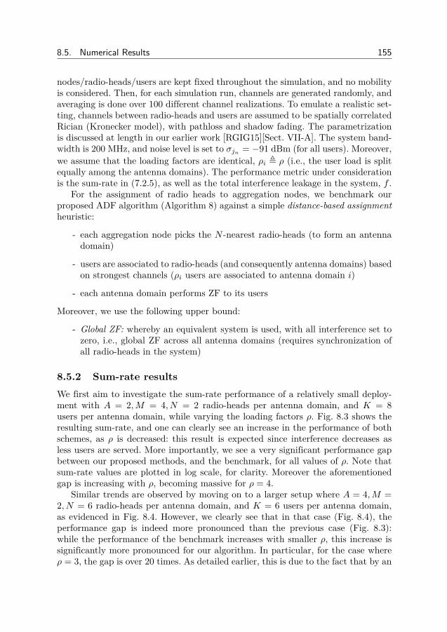
8.5. Numerical Results 155
nodes/radio-heads/users are kept fixed throughout the simulation, and no mobilityis considered. Then, for each simulation run, channels are generated randomly, andaveraging is done over 100 different channel realizations. To emulate a realistic set-ting, channels between radio-heads and users are assumed to be spatially correlatedRician (Kronecker model), with pathloss and shadow fading. The parametrizationis discussed at length in our earlier work [RGIG15][Sect. VII-A]. The system band-width is 200 MHz, and noise level is set to σjn = −91 dBm (for all users). Moreover,we assume that the loading factors are identical, ρi , ρ (i.e., the user load is splitequally among the antenna domains). The performance metric under considerationis the sum-rate in (7.2.5), as well as the total interference leakage in the system, f .
For the assignment of radio heads to aggregation nodes, we benchmark ourproposed ADF algorithm (Algorithm 8) against a simple distance-based assignmentheuristic:
- each aggregation node picks the N -nearest radio-heads (to form an antennadomain)
- users are associated to radio-heads (and consequently antenna domains) basedon strongest channels (ρi users are associated to antenna domain i)
- each antenna domain performs ZF to its users
Moreover, we use the following upper bound:
- Global ZF: whereby an equivalent system is used, with all interference set tozero, i.e., global ZF across all antenna domains (requires synchronization ofall radio-heads in the system)
8.5.2 Sum-rate resultsWe first aim to investigate the sum-rate performance of a relatively small deploy-ment with A = 2,M = 4, N = 2 radio-heads per antenna domain, and K = 8users per antenna domain, while varying the loading factors ρ. Fig. 8.3 shows theresulting sum-rate, and one can clearly see an increase in the performance of bothschemes, as ρ is decreased: this result is expected since interference decreases asless users are served. More importantly, we see a very significant performance gapbetween our proposed methods, and the benchmark, for all values of ρ. Note thatsum-rate values are plotted in log scale, for clarity. Moreover the aforementionedgap is increasing with ρ, becoming massive for ρ = 4.
Similar trends are observed by moving on to a larger setup where A = 4,M =2, N = 6 radio-heads per antenna domain, and K = 6 users per antenna domain,as evidenced in Fig. 8.4. However, we clearly see that in that case (Fig. 8.4), theperformance gap is indeed more pronounced than the previous case (Fig. 8.3):while the performance of the benchmark increases with smaller ρ, this increase issignificantly more pronounced for our algorithm. In particular, for the case whereρ = 3, the gap is over 20 times. As detailed earlier, this is due to the fact that by an

156 Proposed Approach
0 5 10 15 20
100
101
102
Power allocation per RRH (dBm)
Avera
ge s
um
rate
(bits/s
/Hz)
SR M = 4 , A = 2, N = 2, K = 8, Nsim = 20, γ = 4, 5, 6, 7
Proposed ADF
Distance−based assignment
ρ = 6
ρ = 7
ρ = 5
ρ = 4
ρ = 4, 5, 6, 7
Figure 8.3: Average sum-rate performance for A = 2,M = 4, N = 2,K = 8
appropriate choice of ρ, the proposed scheme can totally suppress all interferencein the system.
To shed further light on the latter effect, we investigated further deploymentswith A = 2, N = 2, K = MN , and where the loading factor is appropriately chosenas ρ = K/2. Fig. 8.5 shows the sum-rate for such a system, for various values ofM . Most importantly, in this regime, our proposed algorithm coincides exactly withthat of the global ZF upper bound. This is due to the fact that all the latter schemesare able to totally suppress all interference in the network.
8.5.3 Performance bounds
We compare in this section, the performance of the proposed BCD algorithm (Algo-rithm 7), against the globally optimal solution (found via exhaustive search), as wellas the DW lower bound. We first look at the tightness of the DW decomposition,with respect to the globally optimal solution of (P ). We consider a small scenario(A = 2), assuming no fading, and looking at the (average) total interference leakagef , as metric. As seen in Table 8.2, the error form approximating the globally optimalsolution of (P ), by the DW lower bound (solved using CGM in Table 8.1) is quitetolerable (for ρ = 3, 4). We note that the case where ρ = 1 is too small, and notpractically relevant. We also compare in Table 8.2 the performance of the proposedBCD algorithm (Algorithm 7) against that of the globally optimal solution. Withthat in mind, we observe a similar trend here, where the proposed BCD algorithm
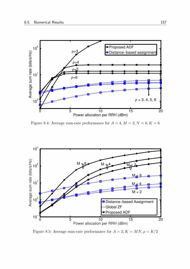
8.5. Numerical Results 157
0 5 10 15 20
100
101
102
Power allocation per RRH (dBm)
Avera
ge s
um
rate
(bits/s
/Hz)
SR M = 2 , A = 4, N = 6, K = 6, Nsim = 10, γ = 6, 5, 4, 3
Proposed ADF
Distance−based assignmentρ=3
ρ=4
ρ=5
ρ=6
ρ = 3, 4, 5, 6
Figure 8.4: Average sum-rate performance for A = 4,M = 2, N = 6,K = 6
0 5 10 15 2010
−1
100
101
102
103
Power allocation per RRH (dBm)
Avera
ge s
um
rate
(bits/s
/Hz)
SR M = [2,4,8] , A = 2, N = 2, K = MN, Nsim = 20, γ = K/2
Distance−based Assignment
Global ZF
Proposed ADF
M = 4
M = 2
M = 2
M = 8
M = 4M = 8
Figure 8.5: Average sum-rate performance for A = 2,K = MN, ρ = K/2
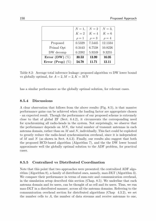
158 Proposed Approach
N = 1, N = 2 N = 3,K = 2 K = 4 K = 6ρ = 1 ρ = 3 ρ = 4
Proposed 0.5329 7.5445 12.1334Primal Opt 0.3443 6.7538 10.8226DW decomp 0.2392 5.9249 9.3255
Error (DW) (%) 30.5330.5330.53 13.9913.9913.99 16.0516.0516.05Error (Prop) (%) 54.7854.7854.78 11.7111.7111.71 12.1112.1112.11
Table 8.2: Average total inference leakage: proposed algorithm vs DW lower boundvs globally optimal, for A = 2,M = 2,K = MN
has a similar performance as the globally optimal solution, for relevant cases.
8.5.4 Discussions
A clear observation that follows from the above results (Fig. 8.5), is that massiveperformance gains can be achieved when the loading factor are appropriate chosen- an expected result. Though the performance of our proposed scheme is extremelyclose to that of global ZF (Sect. 8.4.2), it circumvents the corresponding needfor synchronizing all radio-heads in the system. Not surprisingly, we observe thatthe performance depends on MN , the total number of transmit antennas in eachantenna domain, rather than onM andN , individually. This fact could be exploitedto greatly reduce the radio-head synchronization overhead, since it is independentof M and N (as shown in Sect. 8.4.3). Finally, our results also suggest that boththe proposed BCD-based algorithm (Algorithm 7), and the the DW lower boundapproximate well the globally optimal solution to the ADF problem, for practicalcases.
8.5.5 Centralized vs Distributed Coordination
Note that this point that two approaches were presented: the centralized ADF algo-rithm (Algorithm 8), a family of distributed ones, namely, max-DLT (Algorithm 3).We compare their performance in terms of sum-rate and communication overhead,in the simulation setup described this section (Chap. 8.5). We underline that eachantenna domain and its users, can be thought of as cell and its users. Thus, we runmax-DLT in a distributed manner, across all the antenna domains. Referring to thecommunication overhead section for distributed algorithms (Chap 4.3.2), we setthe number cells to A, the number of data streams and receive antennas to one,

8.6. Conclusion 159
and the resulting communication overhead reduces to,
ΩDIST = 2AKT +AK +AK = 2KTT + 2KT = KT (2T + 2) symbols , (8.5.1)
where T is the number of forward-backward iterations for max-DLT. In the aboveequation, while the first term is the CSI acquisition overhead, the second and thirdterms represent synchronization overhead (among different radio-heads) and datasharing overhead (sharing the data among all the different antenna domains). More-over, recall that the total communication overhead for the ADF algorithm (Algo-rithm 8) was shown to be,
ΩCENT = KT (2 +MN +AL/8) symbols , (8.5.2)
With that in mind, note that ΩDIST ≤ ΩCENT when,
T ≤MN/2 +AL/16 . (8.5.3)
For the low-overhead algorithm that we advocate in this thesis, this is indeed thecase: the overhead of a distributed solution is better than that of its centralizedcounterpart.
We next compare their sum-rate performance, considering a system with A =2,M = 4, N = 2,K = 8. Note that for such as system, ΩDIST = 160 symbols,ΩCENT = 224 symbols. The resulting sum-rates are shown in Fig 8.6. The resultdepends on the SNR, and loading factor ρ. In most of the cases, its seems that max-DLT performs better than the centralized ADF. The only exception is for low-loadcondition ρ = 3, where the ADF solution slightly outperforms the distributed one, inthe high-SNR region only. In addition, note that in the low-to-medium SNR region,distributed solutions (via max-DLT) are always better than the centralized one (viaADF). Thus, one can conclude at this stage that given the communication overheadmodels for max-DLT and the proposed ADF algorithm, distributed approaches suchas max-DLT offer better performance, with a lower overhead (this conclusion isheavily dependent on the communication overhead models). Moving to a larger anddenser setting (Fig. 8.7), we observe the same trends described just above, where theperformance gap between max-DLT and the ADF algorithm is more pronounced.However, we recall that our overhead models (for the proposed ADF method andmax-DLT), are not fully comprehensive and do not model all the required overhead.Thus, the above conclusion holds for the overhead models in question : it does nothold for any real system. Note in addition, that approaches such as max-DLT havethe additional advantage of taking both the signal and interference into account,whereas the proposed ADF solely relies on the interference leakage.
8.6 Conclusion
We formulated the ADF problem as an integer optimization problem (using theinterference leakage at metric), and showed that it can be tackled using BCD. Mo-tivated by the complicated nature of the problem, we argued the need for “good”
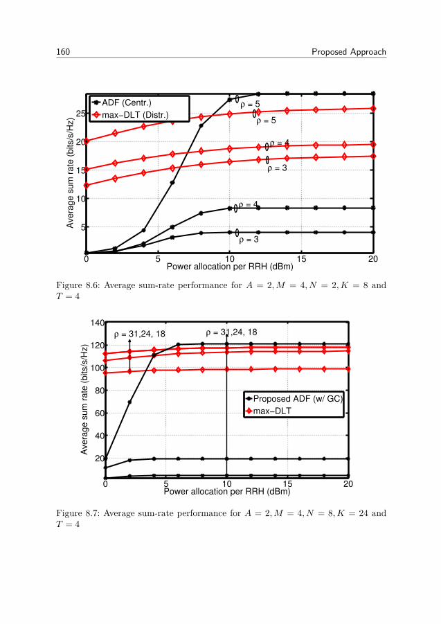
160 Proposed Approach
0 5 10 15 20
5
10
15
20
25
Power allocation per RRH (dBm)
Avera
ge s
um
ra
te (
bits/s
/Hz)
SR M = 4 , A = 2, N = 2, K = 8, Nsim = 50, ρ = 5,6,7
ADF (Centr.)
max−DLT (Distr.)ρ = 5
ρ = 5
ρ = 4
ρ = 4
ρ = 3
ρ = 3
Figure 8.6: Average sum-rate performance for A = 2,M = 4, N = 2,K = 8 andT = 4
0 5 10 15 20
20
40
60
80
100
120
140
Power allocation per RRH (dBm)
Avera
ge s
um
rate
(bits/s
/Hz)
SR M = 4 , A = 2, N = 8, K = 32, Nsim = 30, γ =31, 24, 18
Proposed ADF (w/ GC)
max−DLT
ρ = 31,24, 18 ρ = 31,24, 18
Figure 8.7: Average sum-rate performance for A = 2,M = 4, N = 8,K = 24 andT = 4

8.7. Appendix 161
lower bounds on the problem (as well as the interference leakage). We investigatedseveral “classical” lower bounds, such as the DW decomposition, the dual problem,and showed that the DW lower bound is tighter. Due to the exponential numberof variables present in the DW lower bound, we adapted the Column GenerationMethod to (globally) solve it. Finally, sum-rate results clearly indicate a large per-formance gap between our proposed ADF algorithm, and the relevant benchmark.Moreover, in practical setups, the proposed ADF algorithm, and the advocatedlower bound, seem approximate the optimal solution to the ADF problem, withacceptable error.
8.7 Appendix
8.7.1 Proof of Proposition 7.3.1The fact that (P ) can be rewritten in vector form, i.e., (7.3.2), is straightforwardand can be skipped. As for rewriting (P ) in matrix form (7.3.3), we first recall thatfor any QQQ ∈ Rm×m, 111TmQQQ111m =
∑mi=1∑mj=1Qi,j , and rewrite the cost function in
(P ) as,
f = tr[111TA(XXXTΨΨΨXXX)111A]− tr(XXXTΨΨΨXXX)
= tr(XXXTΨΨΨXXX111A111TA)− tr(XXXTΨΨΨXXX) = tr(XXXTΨΨΨXXXΩΩΩ
), (8.7.1)
where we used the fact that tr(AAABBB) = tr(BBBAAA), and let ΩΩΩ , 111A111TA − IIIA. Moreover,the loading constraint can be rewritten as,∑
im
xk,im = ρk, ∀k ⇔ 111TKTXXX = [ρ1, ..., ρA]⇔XXXT111N = ρρρ.
Similarly, the assignment constraint can be reformulated as,
A∑k=1
xk,im ≤ 1,∀im ∈ I ⇔XXX111A ≤ 111KT .
8.7.2 Proof of Proposition 8.1.1Note that (8.1.8) is a convex problem (quadratic cost and linear constraint), it canbe solved using standard Lagrangian techniques. The associated Lagrangian is,
L(VVV i,MMM i) = tr(VVV †iRRRiVVV i) + tr [MMM i(HHHi,iVVV i − βiIIIdi)] ,
whereMMM i ∈ Cdi×di is the matrix of Lagrange multipliers. Differentiating the latterw.r.t. VVV i and setting to zero yields,
∇VVV iL = 000⇔ VVV ?i = −RRR−1i HHH†i,iMMM
?i ,

162 Proposed Approach
where MMM?i is chosen to satisfy the linear constraint, i.e.,
HHHi,i(−RRR−1i HHH†i,iMMM
?i ) = βiIIIdi ⇔MMM?
i = −βi(HHHi,iRRR−1i HHH†i,i)
−1.
Combining the last two equations yields the optimal solution,
VVV ?i = βi RRR−1i HHH†i,i
(HHHi,iRRR
−1i HHH†i,i
)−1.
The resulting transmit power is
‖VVV ?i ‖2F = β2i ‖RRR
−1i HHH†i,i
(HHHi,iRRR
−1i HHH†i,i
)−1‖2F .
Thus transmit power constraint is satisfied with equality for
βi =√di/‖RRR−1
i HHH†i,i
(HHHi,iRRR
−1i HHH†i,i
)−1‖F .
Note that when di ≤ MN , then there always exists at least one VVV i, such thatHHHi,iVVV i = βiIIIdi : the Moore-Penrose inverse of HHHi,i/βi. Due to the generic natureof the channels, HHHi,i/βi is full-rank almost surely, its Moore-Penrose inverse existsalmost surely, and the problem is feasible almost surely.
8.7.3 Proof of Lemma 8.3.1The proof follows from considering the following “DW-like” mapping,
S = ZZZ =∑j
tjWWW j |∑j
tj = 1, tj ∈ B ,∀j = 1, ..., n
= ZZZ =∑j
tjWWW j | tttT111n = 1, ttt ∈ Bn. (g.1)
Then, the cost in (Q) is written as p(ZZZ) =∑j tjp(WWW j). Letting ttt = [t1, ..., tn]T ,
and θj = p(WWW j), (Q) is equivalent to,
(Q)argmin pd(ttt) = tttTθθθ
s. t. tttT111n = 1, ttt ∈ Bn.(8.7.2)
It can be verified that the mapping in (g.1) is one-to-one from Z to ttt: every ttt yieldsa unique ZZZ, and every ZZZ decomposes into a unique ttt. The equivalence between thetwo problems follows from that.
8.7.4 Proof of Lemma 8.1.1Note that the following is a direct consequence of (8.1.3)
f(xxx(n)k ) ≥ f(xxx(n+1)
1 , zzz(n)1 ) ≥ f(xxx(n+1)
2 , zzz(n)2 )...
≥ f(xxx(n+1)A , zzz
(n)A ) , f(xxx(n+1)
k ),

8.7. Appendix 163
where the last equality follows from the fact that f(xxx(n+1)A , zzz
(n)A ) corresponds to
the case where all variables (xxx1, ....,xxxA), are updated. It follows that the sequencef(xxx(n)
1 , ...,xxx(n)A )n converges to a limit point f0
8.7.5 Proof of Lemma 8.2.1Let η =
∑k
∑l 6=k ρkρl. The left inequality follows immediately from the fact that
the DW decomposition is always a lower bound on the problem - by construction(Sec 8.2.2). Moreover, the right one is obtained from upper bounding f(XXX?) andlower bounding fDW (www?),
f(XXX?) =∑k
∑l 6=k
xxx?T
k ΨΨΨxxx?l ≤∑k
∑l 6=k
σmax[ΨΨΨ]‖xxx?k‖2‖xxx?l ‖2
(e.1)= σmax[ΨΨΨ]∑k
∑l 6=k
ρkρl = σmax[ΨΨΨ]η
where (e.1) follows from the fact that xxx?k must be feasible: thus, ‖xxx?k‖2 is the sum ofall non-zero elements, and equal to ρk. Moreover, a simple/naive lower bound canbe obtained on PDW in (8.2.8), by relaxing the first constraint,
fDW (www?) ≥ min111TSwww=1,www≥000S
αααTwww(e.1)= min
1≤j≤Sαj = min
jtr(QQQTj ΨΨΨQQQjΩΩΩ)
(e.2)≥ ησmin[ΨΨΨ]
where (e.1) follows from the fact that problem in a special LP, whose solutionis obtained in Definition 8.2.2. Moreover, (e.2) follows similar reasoning used forlower bounding d(λλλ?) in Appendix 8.7.7. The first and second bound follows fromcombining (e.1) and (e.2) respectively.
8.7.6 Proof of Proposition 8.2.1We rewrite (8.2.15) in a series of equivalent problems,
(D) maxλλλ≥000KT
d(λλλ) = minQQQj∈Sρ
tr(QQQTj ΨΨΨQQQjΩΩΩ) + λλλT (QQQj111A − 111KT )
(D) maxλλλ≥000KT
d(λλλ) = min1≤j≤S
αj + λλλTqqqj
(D)
maxλλλ≥000KT , ζ
ζ
s. t. αj + λλλTqqqj ≥ ζ, ∀j = 1, · · · , S
(D)
maxλλλ,ζ
ζ
s. t. ααα+ ΓΓΓTλλλ ≥ ζ111S , λλλ ≥ 000KT
The result in (8.2.16) follows by letting µµµ = [λλλ, ζ]T , ccc = [000N , 1]T , and ΓΓΓT =[−ΓΓΓT , 111S ].

164 Proposed Approach
8.7.7 Proof of Lemma 8.2.2Let η =
∑k
∑l 6=k ρkρl. The left inequality, stating that the dual solution is always
a lower bound on the primal one, follows immediately from weak duality. Moreover,the right one is obtained from upper bounding f(XXX?) and lower bounding d(λλλ?),
f(XXX?) =∑k
∑l 6=k
xxx?T
k ΨΨΨxxx?l ≤∑k
∑l 6=k
σmax[ΨΨΨ]‖xxx?k‖2‖xxx?l ‖2,
(e.1)= σmax[ΨΨΨ]∑k
∑l 6=k
ρkρl = σmax[ΨΨΨ]η,
where (e.1) follows from the fact that xxx?k must be feasible: thus, ‖xxx?k‖2 is the sumof all non-zero elements, and equal to ρk. Using (8.2.15), we formulate the optimaldual solution (and its lower bound) as,
d(λλλ?)
, minXXX∈Sρ
tr(XXXTΨΨΨXXXΩΩΩ) + λλλ?T
(XXX111A − 111KT )
= minxxxk∈BKT ,∀kxxxTk 111KT =ρk,∀k
∑k
xxxTk
∑l 6=k
ΨΨΨxxxl + λλλ?
− 111TKTλλλ?
≥ minxxxk∈BKT ,∀kxxxTk 111KT =ρk,∀k
∑k
∑l 6=k
(σmin[ΨΨΨ]‖xxxk‖2‖xxxl‖2) + xxxTkλλλ?
− 111TKTλλλ?
(e.2)= σmin[ΨΨΨ]η − 111TKTλλλ? +
∑k
minxxxk∈BKTxxxTk 111KT =ρk
xxxTkλλλ?
(e.3)= σmin[ΨΨΨ]η − 111TKTλλλ? +
∑k
minxxxk≥000
xxxTk 111KT =ρk
xxxTkλλλ?
(e.4)= σmin[ΨΨΨ]η − 111TKTλλλ? +
∑k
ρk
minzzzk≥000
zzzTk 111KT =1
zzzTkλλλ?
(e.5)= σmin[ΨΨΨ]η − 111TKTλλλ
? +∑k
ρk mini
[λλλ?]i.
Note that (e.2) follows from the fact that ‖xxxk‖2 = ρk for any feasible xxxk. (e.3) isdue to the fact that the problem is a MILP. Furthermore, we show that it satisfiedthe integrality property (as per Definition 8.1.1): then, relaxing the binary con-straint into a continuous one, yields the optimal solution. Finally, (e.4) is obtainedby letting zzzk = xxxk/ρk, and (e.5) from the fact that the problem is a Special LPwhose solution is detailed in Definition 8.2.2. The final result follows by combiningthe above result with (e.1).

8.7. Appendix 165
8.7.8 Proof of Corollary 8.4.1Let ZZZi ,
⋃j 6=i
span(HHHi,j), and NNN i = null(ZZZi). Due to the generic random nature of
the channels, then one can verify that dim(NNN i) = MN − ρi, almost surely. In thecase where
∑i ρi ≤MN , then
dim(NNN i) ≥ ρi ⇔ ∃ TTT i ∈ CMN×ρi ,TTT i ∈NNN i
⇔ ∃ TTT i ∈ CMN×ρi ,TTT †iHHHi,j = 000ρi×ρi , ∀j 6= i,
⇔ ∃ TTT i ∈ CMN×ρi ,TTT †iRRRiTTT i = 000ρi×ρi
Note that h(VVV i) ≥ 0, since it is a quadratic form. Moreover, since the problemis convex and has a unique optimal solution, any solution that makes h zero, isglobally optimal then. Then, consider solutions of the form, VVV i = TTT iΘΘΘi, where ΘΘΘi
is an arbitrary unitary matrix. Then,
h(VVV i) = tr(ΘΘΘ†iTTT†iRRRiTTT iΘΘΘi) = tr(TTT †iRRRiTTT i) = 0

Chapter 9
Conclusions and Future Work
In this thesis, we have investigated optimization techniques for the most promis-ing communication systems. Our contributions have addressed all three pillarsfor increasing data rates in cellular systems, namely, (A) exploiting the massive
spectrum of mmWave MIMO systems, (B) increasing the spectral efficiency via BScoordination, and (C) densification.
Under (A), we motivated the hybrid analog-digital MIMO architecture as a keyto scaling up the number of transmit/receive antennas for mmWave MIMO systems.After characterizing the optimal precoder/combiner structure, we proposed an algo-rithm (based on the Arnoldi Iteration) to blindly estimate the dominant subspacesof the mmWave MIMO channel. This is motivated by the fact the such channelsare inherently sparse (in terms of eigenmodes): it is much more efficient to estimatethe non-zero eigenmodes, rather than the entire channel. In addition, we also de-vised an iterative procedure to optimize the analog/digital precoder and combiner(based on estimates of the dominant subspace). Simulation results showed that theproposed approach significantly outperforms the only benchmark. We believe thatsuch an approach - subspace estimation exploiting channel reciprocity (or later onesthat build upon it), will be an essential component in the operation of mmWaveMIMO systems. The above approach assumes narrow-band channels: this is hardto motivate, since mmWave MIMO systems have a large bandwidth, and are thusinherently frequency selective. In the future, we consider extending the proposedsubspace estimation approach, to handle wide-band frequency selective channels.Moreover, we also envision to reduce the communication overhead resulting fromthe Arnoldi iteration.
Under (B), we investigated algorithms for distributed multi-user multi-cell co-ordination, under the framework of F-B iterations. Despite the plethora of differentapproaches developed over the years, we highlighted the fact that they all requireda large enough number of iterations that would destroy the gains brought about bytheir use: we thus proposed two types of low-overhead algorithms that require justa few F-B iterations. In the first algorithm, max-DLT, we lower bounded the sum-rate using a so-called DLT bound, and derived the corresponding solution, dubbedas non-homogeneous waterfilling: we highlighted its ability to turn off streams with
167

168 Conclusions and Future Work
low-SINR, thereby greatly speeding up the convergence of the algorithm. In thesecond type of algorithm, we used the interference leakage as metric. The increasedconvergence speed is due firstly due to relaxing the leakage minimization problem,and the introduction of a turbo iteration at the transmitters/receivers, within eachF-B iteration, where the leakage is further decreased.
In (C), we focused on the opposing paradigm of fully centralized coordination,given by the Cloud-RAN architecture - the most prominent candidate for den-sification. In the case of multiple antenna domains, we highlighted the absenceof prior work tackling both intra-AD and inter-AD interference, and formulatedthe so-called antenna domain formation problem, using the interference leakage asmetric. We proposed an iterative algorithm, based on Block Coordinate Descent,to solve it. Motivated by the lack of theoretical guarantees on the optimality ofsuch a solution, we derived lower bounds on the problem (and the interferenceleakage consequently), and compared them analytically. We also compared the per-formance of the proposed (centralized) ADF algorithm to (distributed) max-DLT(in the same Cloud-RAN simulation setup), and concluded that the low-overheadfast-converging max-DLT outperformed the centralized ADF algorithm. We alsonoticed that this performance gap increases as the deployment gets denser. We ar-gued that this result is valid for the particular communication overhead model usedhere. We thus conclude at this point, that for the algorithms and communicationscenarios considered in this thesis, distributed coordination algorithms (with focusof fast-convergence), are a clear winner in the case of densification. In the future,we plan to extend the numerical setup considered here, to include basic mobilityof the users. We wish to investigate the robustness of the proposed ADF approachto changes in user positions, resulting from mobility: How is the sum-rate affected,if the ADF algorithms is run at higher intervals? In addition, metrics includingfairness will also be considered.

Bibliography
[3GP11] Spatial channel model for multiple input multiple output (MIMO)simulations. 3GPP TR 25.996 V10.0, Mar 2011.
[AEALH14] A. Alkhateeb, O. El Ayach, G. Leus, and R.W. Heath. Channel es-timation and hybrid precoding for millimeter wave cellular systems.IEEE Journal of Selected Topics in Signal Processing, 8(5):831–846,Oct 2014.
[AEB06] M. Aharon, M. Elad, and A Bruckstein. K-SVD: An algorithm fordesigning overcomplete dictionaries for sparse representation. IEEETransactions on Signal Processing, 54(11):4311–4322, Nov 2006.
[AHAS+12] O.E. Ayach, R.W. Heath, S. Abu-Surra, S. Rajagopal, and ZhouyuePi. Low complexity precoding for large millimeter wave MIMO sys-tems. In Communications (ICC), 2012 IEEE International Confer-ence on, pages 3724–3729, June 2012.
[BB11] D.S. Baum and H. Bolcskei. Information-theoretic analysis of MIMOchannel sounding. Information Theory, IEEE Transactions on,57(11):7555–7577, Nov 2011.
[BB15a] R. Brandt and M. Bengtsson. Distributed CSI acquisition and coor-dinated precoding for TDD multicell MIMO systems. IEEE Trans-actions on Vehicular Technology, PP(99):1–1, 2015.
[BB15b] R. Brandt and M. Bengtsson. Fast-convergent distributed coordi-nated precoding for TDD multicell MIMO systems. In Computa-tional Advances in Multi-Sensor Adaptive Processing (CAMSAP),2015 IEEE 6th International Workshop on, pages 457–460, Dec2015.
[BE06] Amir Beck and Yonina Eldar. Strong duality in nonconvex quadraticoptimization with two quadratic constraints. SIAM Journal on Op-timization, 17(3):844–860, 2006.
[Ben02] M. Bengtsson. A pragmatic approach to multi-user spatial multi-plexing. In Sensor Array and Multichannel Signal Processing Work-shop Proceedings, 2002, pages 130–134, Aug 2002.
169
170 Bibliography
[Bis06] Christopher M. Bishop. Pattern Recognition and Machine Learning(Information Science and Statistics). Springer-Verlag New York,Inc., Secaucus, NJ, USA, 2006.
[BJBO11] E. Bjornson, N. Jalden, M. Bengtsson, and B. Ottersten. Optimal-ity properties, distributed strategies, and measurement-based eval-uation of coordinated multicell ofdma transmission. IEEE Transac-tions on Signal Processing, 59(12):6086–6101, Dec 2011.
[BJN+96] Cynthia Barnhart, Ellis L. Johnson, George L. Nemhauser, Mar-tin W. P. Savelsbergh, and Pamela H. Vance. Branch-and-price:Column generation for solving huge integer programs. OperationsResearch, 46:316–329, 1996.
[Bra83] D. H. Brandwood. A complex gradient operator and its applicationin adaptive array theory. IEE Proceedings Communications, Radarand Signal Processing, 130(1):11–16, 1983.
[BV04] Stephen Boyd and Lieven Vandenberghe. Convex Optimization.Cambridge University Press, New York, NY, USA, 2004.
[CJ08] V.R. Cadambe and S.A. Jafar. Interference alignment and degreesof freedom of the K -user interference channel. IEEE Transactionson Information Theory, 54(8):3425–3441, 2008.
[CJ09] V. R Cadambe and S. A Jafar. Reflections on interference alignmentand the degrees of freedom of the k-user mimo interference channel.IEEE Information Theory Society Newsletter, 54(4):5–8, December2009.
[CKGB16] W. M. Chan, T. Kim, H. Ghauch, and M. Bengtsson. Subspace es-timation and hybrid precoding for wideband millimeter-wave mimosystems. IEEE ASILOMAR, Nov. 2016.
[CTRF02] J.-H. Chang, L. Tassiulas, and F. Rashid-Farrokhi. Joint transmit-ter receiver diversity for efficient space division multiaccess. IEEETransactions on Wireless Communications, 1(1):16–27, Jan 2002.
[DCG04] T. Dahl, N. Christophersen, and D. Gesbert. Blind MIMO eigen-mode transmission based on the algebraic power method. IEEETransactions on Signal Processing, 52(9):2424–2431, Sept 2004.
[DHL+11] M. Dohler, R. W. Heath, A. Lozano, C. B. Papadias, and R. A.Valenzuela. Is the phy layer dead? IEEE Communications Magazine,49(4):159–165, April 2011.

Bibliography 171
[DPCG07] T. Dahl, S.S. Pereira, N. Christophersen, and D. Gesbert. Intrinsicsubspace convergence in TDD MIMO communication. IEEE Trans-actions on Signal Processing, 55(6):2676–2687, June 2007.
[DY16] Binbin Dai and Wei Yu. Energy efficiency of downlink transmissionstrategies for cloud radio access networks. CoRR, abs/1601.01070,2016.
[EALH11] O. El Ayach, A. Lozano, and R.W. Heath. Optimizing training andfeedback for MIMO interference alignment. In Conference Recordof the Forty Fifth Asilomar Conference on Signals, Systems andComputers (ASILOMAR), pages 1717–1721, 2011.
[EALH12] O. El Ayach, A. Lozano, and R.W. Heath. On the overhead ofinterference alignment: Training, feedback, and cooperation. IEEETransactions on Wireless Communications, 11(11):4192–4203, 2012.
[EARAS+14] O. El Ayach, S. Rajagopal, S. Abu-Surra, Zhouyue Pi, andR.W. Heath. Spatially sparse precoding in millimeter waveMIMO systems. IEEE Transactions on Wireless Communications,,13(3):1499–1513, March 2014.
[Eri15] On the pulse of the networked society. Ericsson Mobility Report,November 2015.
[Fra05] Antonio Frangioni. About lagrangian methods in integer optimiza-tion. Annals of Operations Research, 139(1):163–193, 2005.
[GBD60a] Philip Wolfe George B. Dantzig. Decomposition principle for linearprograms. Operations Research, 8(1):101–111, 1960.
[GBD60b] Philip Wolfe George B. Dantzig. Decomposition principle for linearprograms. Operations Research, 8(1):101–111, 1960.
[GBKS15] H. Ghauch, M. Bengtsson, T. Kim, and M. Skoglund. Subspaceestimation and decomposition for hybrid analog-digital millimetre-wave mimo systems. In 2015 IEEE 16th International Workshop onSignal Processing Advances in Wireless Communications (SPAWC),pages 395–399, June 2015.
[GCJ11] K. Gomadam, V. R Cadambe, and S. A Jafar. A distributed numer-ical approach to interference alignment and applications to wirelessinterference networks. IEEE Transactions on Information Theory,57(6):3309–3322, June 2011.
[GHH+10] D. Gesbert, S. Hanly, H. Huang, S. Shamai Shitz, O. Simeone, andWei Yu. Multi-cell MIMO cooperative networks: A new look atinterference. IEEE Journal on Selected Areas in Communications,28(9):1380–1408, 2010.

172 Bibliography
[GKBS13] H. Ghauch, T. Kim, M. Bengtsson, and M. Skoglund. Interfer-ence alignment via controlled perturbations. In 2013 IEEE GlobalCommunications Conference (GLOBECOM), pages 3996–4001, Dec2013.
[GKBS15] H. Ghauch, Taejoon Kim, M. Bengtsson, and M. Skoglund. Dis-tributed low-overhead schemes for multi-stream MIMO interferencechannels. IEEE Transactions on Signal Processing, 63(7):1737–1749,April 2015.
[GKBS16a] H. Ghauch, T. Kim, M. Bengtsson, and M. Skoglund. Subspace esti-mation and decomposition for large millimeter-wave mimo systems.IEEE Journal of Selected Topics in Signal Processing, 10(3):528–542, April 2016.
[GKBS16b] H. Ghauch, Taejoon Kim, M. Bengtsson, and M. Skoglund. Sepa-rability and sum-rate maximization in MIMO interfering networks.IEEE Transactions on Signal and Information Processing over Net-works, Submitted , available at http://arxiv.org/pdf/1606.08589.pdf,2016.
[GMBS15] H. Ghauch, R. Mochaourab, M. Bengtsson, and M. Skoglund. Dis-tributed precoding and user selection in mimo interfering networks.In Computational Advances in Multi-Sensor Adaptive Processing(CAMSAP), 2015 IEEE 6th International Workshop on, pages 461–464, Dec 2015.
[GP11] H.G. Ghauch and C.B. Papadias. Interference alignment: A one-sided approach. In 2011 IEEE Global Communications Conference(GLOBECOM 2011), pages 1 –5, December 2011.
[GRI+16] H. Ghauch, M. M. U. Rahman, S. Imtiaz, J. Gross, M. Skoglund,and C. Qvarfordt. Performance bounds for antenna domain systems.IEEE Transactions on Signal Processing, Submitted , available athttp://arxiv.org/pdf/1606.08401.pdf, 2016.
[GRIG16] H. Ghauch, M. Rahman, S. Imtiaz, and J. Gross. Coordination andantenna domain formation in Cloud-RAN systems. IEEE Interna-tional Communications Conference ICC, 2016.
[GVL96] Gene H. Golub and Charles F. Van Loan. Matrix computations (3rded.). Johns Hopkins University Press, Baltimore, MD, USA, 1996.
[HDMF10] T. Hrycak, S. Das, G. Matz, and H.G. Feichtinger. Low complex-ity equalization for doubly selective channels modeled by a basisexpansion. IEEE Transactions on Signal Processing, 58(11):5706–5719, Nov 2010.

Bibliography 173
[HKG+14] J. He, T. Kim, H. Ghauch, K. Liu, and G. Wang. Millimeter wavemimo channel tracking systems. In 2014 IEEE Globecom Workshops(GC Workshops), pages 416–421, Dec 2014.
[HKL+13] Sooyoung Hur, Taejoon Kim, D.J. Love, J.V. Krogmeier, T.A.Thomas, and A. Ghosh. Millimeter wave beamforming for wire-less backhaul and access in small cell networks. Communications,IEEE Transactions on, 61(10):4391–4403, October 2013.
[HRLP16] M. Hong, M. Razaviyayn, Z. Q. Luo, and J. S. Pang. A unified algo-rithmic framework for block-structured optimization involving bigdata: With applications in machine learning and signal processing.IEEE Signal Processing Magazine, 33(1):57–77, Jan 2016.
[HXRL13] Mingyi Hong, Zi Xu, M. Razaviyayn, and Zhi-Quan Luo. Joint usergrouping and linear virtual beamforming: Complexity, algorithmsand approximation bounds. IEEE Journal on Selected Areas inCommunications,, 31(10):2013–2027, October 2013.
[KFVY06] M.K. Karakayali, G.J. Foschini, R. Valenzuela, and R.D. Yates. Onthe maximum common rate achievable in a coordinated network. InCommunications, 2006. ICC ’06. IEEE International Conferenceon, volume 9, pages 4333–4338, June 2006.
[KG11] S. J. Kim and G. B. Giannakis. Optimal resource allocation forMIMO ad hoc cognitive radio networks. IEEE Transactions on In-formation Theory, 57(5):3117–3131, May 2011.
[KTJ12] J. Kaleva, A. Tölli, and M. Juntti. Weighted sum rate maximiza-tion for interfering broadcast channel via successive convex approx-imation. In Global Communications Conference (GLOBECOM),2012 IEEE, pages 3838–3843, Dec 2012.
[KTJ13] P. Komulainen, A. Tolli, and M. Juntti. Effective CSI signalingand decentralized beam coordination in TDD multi-cell MIMO sys-tems. IEEE Transactions on Signal Processing, 61(9):2204–2218,May 2013.
[LB15] Thomas Lipp and Stephen Boyd. Variations and extension of theconvex–concave procedure. Optimization and Engineering, pages1–25, 2015.
[LD05] Marco Lubbecke and Jacques Desrosiers. Selected topics in columngeneration. Oper. Res., 53(6):1007–1023, 2005.
[LH03] D.J. Love and R.W. Heath. Equal gain transmission in multiple-input multiple-output wireless systems. Communications, IEEETransactions on, 51(7):1102–1110, July 2003.

174 Bibliography
[LHA13] A. Lozano, R.W. Heath, and J.G. Andrews. Fundamental lim-its of cooperation. IEEE Transactions on Information Theory,59(9):5213–5226, Sept 2013.
[LHMJL13] Namyoon Lee, R.W. Heath, D. Morales-Jimenez, and A. Lozano.Base station cooperation with dynamic clustering in super-densecloud-RAN. In Globecom Workshops (GC Wkshps), 2013 IEEE,pages 784–788, Dec 2013.
[LMS+10] Zhi-Quan Luo, Wing-Kin Ma, A.M.-C. So, Yinyu Ye, and ShuzhongZhang. Semidefinite relaxation of quadratic optimization problems.IEEE Signal Processing Magazine,, 27(3):20–34, May 2010.
[LSC+12] Daewon Lee, Hanbyul Seo, B. Clerckx, E. Hardouin, D. Mazzarese,S. Nagata, and K. Sayana. Coordinated multipoint transmissionand reception in lte-advanced: deployment scenarios and operationalchallenges. IEEE Communications Magazine, 50(2):148–155, Febru-ary 2012.
[LY73] David G. Luenberger and Yinyu Ye. Linear and Nonlinear Program-ming. Springer Publishing Company, Incorporated, 1973.
[MAMK08] M.A. Maddah-Ali, A.S. Motahari, and A.K. Khandani. Communi-cation over MIMO X channels: Interference alignment, decomposi-tion, and performance analysis. IEEE Transactions on InformationTheory, 54(8):3457 –3470, August 2008.
[MBGB15] R. Mochaourab, R. Brandt, H. Ghauch, and M. Bengtsson.Overhead-aware distributed csi selection in the mimo interferencechannel. In Signal Processing Conference (EUSIPCO), 2015 23rdEuropean, pages 1038–1042, Aug 2015.
[MET14] METIS D6.2. Initial report on horizontal topics, first results and5G system concept. March 2014.
[MET15] METIS D3.3. Final performance results and consolidated view onthe most promising multi-node/multi-antenna transmission tech-nologies. Feb 2015.
[MNM11] P. Mohapatra, K. E. Nissar, and C.R. Murthy. Interference align-ment algorithms for the k user constant MIMO interference chan-nel. IEEE Transactions on Signal Processing, 59(11):5499–5508,Nov 2011.
[MRRGPH15] R. Mendez-Rial, C. Rusu, N. Gonzalez-Prelcic, and R.W. Heath.Dictionary-free hybrid precoders and combiners for mmwave mimo
Bibliography 175
systems. In Signal Processing Advances in Wireless Communica-tions (SPAWC), 2015 IEEE 16th International Workshop on, pages151–155, June 2015.
[NBH10] J. Nsenga, A. Bourdoux, and F. Horlin. Mixed analog/digital beam-forming for 60 GHz MIMO frequency selective channels. In Com-munications (ICC), 2010 IEEE International Conference on, pages1–6, May 2010.
[NLN14] D. H. N. Nguyen and T. Le-Ngoc. Sum-rate maximization in themulticell MIMO multiple-access channel with interference coordina-tion. IEEE Transactions on Wireless Communications, 13(1):36–48,January 2014.
[NSGS10] F. Negro, S.P. Shenoy, I. Ghauri, and D.T.M. Slock. On the MIMOinterference channel. In Information Theory and Applications Work-shop (ITA), 2010, pages 1–9, Jan 2010.
[OBB+14] A. Osseiran, F. Boccardi, V. Braun, K. Kusume, P. Marsch,M. Maternia, O. Queseth, M. Schellmann, H. Schotten, H. Taoka,H. Tullberg, M. A. Uusitalo, B. Timus, and M. Fallgren. Scenariosfor 5g mobile and wireless communications: the vision of the metisproject. IEEE Communications Magazine, 52(5):26–35, May 2014.
[OMI+03] K. Ohata, K. Maruhashi, M. Ito, S. Kishimoto, K. Ikuina,T. Hashiguchi, K. Ikeda, and N. Takahashi. 1.25 Gbps wireless Gi-gabit ethernet link at 60 GHz-band. In Radio Frequency IntegratedCircuits (RFIC) Symposium, 2003 IEEE, pages 509–512, June 2003.
[OMM+00] K. Ohata, K. Maruhashi, Jun-ichi Matsuda, M. Ito, W. Domon,and S. Yamazaki. A 500Mbps 60GHz-band transceiver for IEEE1394 wireless home networks. In Microwave Conference, 2000. 30thEuropean, pages 1–4, Oct 2000.
[pet09] Interference alignment via alternating minimization. In IEEE In-ternational Conference on Acoustics, Speech and Signal Processing,2009. ICASSP 2009, pages 2445–2448. IEEE, April 2009.
[PH11] S. W Peters and R. W Heath. Cooperative algorithms for MIMOinterference channels. IEEE Transactions on Vehicular Technology,60(1):206–218, January 2011.
[PH12] S.W. Peters and R.W. Heath. User partitioning for less overheadin MIMO interference channels. IEEE Transactions on WirelessCommunications, 11(2):592 –603, February 2012.
176 Bibliography
[Pri03] R.E. Prieto. A general solution to the maximization of the multidi-mensional generalized rayleigh quotient used in linear discriminantanalysis for signal classification. In Acoustics, Speech, and SignalProcessing, 2003. Proceedings. (ICASSP ’03). 2003 IEEE Interna-tional Conference on, volume 6, pages VI–157–60 vol.6, April 2003.
[RGIG15] M. M. U. Rahman, H. Ghauch, S. Imtiaz, and J. Gross. RRH clus-tering and transmit precoding for interference-limited 5G CRANdownlink. In IEEE Globecom Workshops (GC Wkshps), pages 1–7,Dec 2015.
[RHL12] Meisam Razaviyayn, Mingyi Hong, and Zhi-Quan Luo. A UnifiedConvergence Analysis of Block Successive Minimization Methods forNonsmooth Optimization. SIAM Journal on Optimization, 23(11),sep 2012.
[RLL11] M. Razaviyayn, G. Lyubeznik, and Zhi-Quan Luo. On the degreesof freedom achievable through interference alignment in a MIMO in-terference channel. In Signal Processing Advances in Wireless Com-munications (SPAWC), 2011 IEEE 12th International Workshop on,pages 511–515, June 2011.
[RLL12] M. Razaviyayn, G. Lyubeznik, and Z. Q. Luo. On the degrees of free-dom achievable through interference alignment in a mimo interfer-ence channel. IEEE Transactions on Signal Processing, 60(2):812–821, Feb 2012.
[RSM+13] T.S. Rappaport, Shu Sun, R. Mayzus, Hang Zhao, Y. Azar,K. Wang, G.N. Wong, J.K. Schulz, M. Samimi, and F. Gutierrez.Millimeter wave mobile communications for 5G cellular: It will work!Access, IEEE, 1:335–349, 2013.
[Saa11] Yousef Saad. Numerical Methods for Large Eigenvalue Problems.Manchester University Press, (Second Edition):1–337, 2011.
[SDS+05] Jari Salo, Giovanni Del Galdo, Jussi Salmi, Pekka Kyosti,Marko Milojevic, Daniela Laselva, and Christian Schnei-der. MATLAB implementation of the 3GPP Spatial Chan-nel Model (3GPP TR 25.996). On-line, January 2005.http://www.tkk.fi/Units/Radio/scm/.
[SGHP10a] I. Santamaria, O. Gonzalez, R. W Heath, and S. W Peters. Max-imum sum-rate interference alignment algorithms for MIMO chan-nels. In 2010 IEEE Global Communications Conference (GLOBE-COM 2010), pages 1–6. IEEE, December 2010.

Bibliography 177
[SGHP10b] I. Santamaria, O. Gonzalez, R. W Heath, and S. W Peters. Max-imum sum-rate interference alignment algorithms for MIMO chan-nels. In 2010 IEEE Global Communications Conference (GLOBE-COM 2010), pages 1–6. IEEE, December 2010.
[Sor96] Danny C. Sorensen. Implicitly restarted arnoldi/lanczos methodsfor large scale eigenvalue calculations. Technical report, 1996.
[SRL14] M. Sanjabi, M. Razaviyayn, and Zhi-Quan Luo. Optimal joint basestation assignment and beamforming for heterogeneous networks.IEEE Transactions on Signal Processing, 62(8):1950–1961, April2014.
[SRLH11] Qingjiang Shi, Meisam Razaviyayn, Zhi-Quan Luo, and Chen He.An iteratively weighted MMSE approach to distributed sum-utilitymaximization for a MIMO interfering broadcast channel. IEEETransactions on Signal Processing, 59(9):4331–4340, 2011.
[SSB+09] D.A. Schmidt, Changxin Shi, R.A. Berry, M.L. Honig, and W.Utschick. Minimum mean squared error interference alignment. In2009 Conference Record of the Forty-Third Asilomar Conference onSignals, Systems and Computers, pages 1106 –1110, November 2009.
[SSB+13] D.A Schmidt, Changxin Shi, R.A Berry, M.L. Honig, andW. Utschick. Comparison of distributed beamforming algorithmsfor MIMO interference networks. IEEE Transactions on Signal Pro-cessing, 61(13):3476–3489, July 2013.
[SY15a] F. Sohrabi and W. Yu. Hybrid digital and analog beamformingdesign for large-scale mimo systems. In 2015 IEEE InternationalConference on Acoustics, Speech and Signal Processing (ICASSP),pages 2929–2933, April 2015.
[SY15b] F. Sohrabi and Wei Yu. Hybrid digital and analog beamformingdesign for large-scale mimo systems. In Acoustics, Speech and Sig-nal Processing (ICASSP), 2015 IEEE International Conference on,pages 2929–2933, April 2015.
[SY16] F. Sohrabi and W. Yu. Hybrid digital and analog beamforming de-sign for large-scale antenna arrays. IEEE Journal of Selected Topicsin Signal Processing, 10(3):501–513, April 2016.
[SZ95] K. Schittkowski and C. Zillober. Stochastic Programming: Numer-ical Techniques and Engineering Applications, chapter SequentialConvex Programming Methods, pages 123–141. Springer Berlin Hei-delberg, Berlin, Heidelberg, 1995.

178 Bibliography
[SZ01] S. Shamai and B.M. Zaidel. Enhancing the cellular downlink capac-ity via co-processing at the transmitting end. In Vehicular Technol-ogy Conference, 2001. VTC 2001 Spring. IEEE VTS 53rd, volume 3,pages 1745–1749 vol.3, 2001.
[TCZY15] Meixia Tao, Erkai Chen, Hao Zhou, and Wei Yu. Content-centricsparse multicast beamforming for cache-enabled cloud RAN. CoRR,abs/1512.06938, 2015.
[TO02] M. Torlak and O. Ozdemir. A Krylov subspace approach to blindchannel estimation for CDMA systems. In Signals, Systems andComputers, 2002. Conference Record of the Thirty-Sixth AsilomarConference on, volume 1, pages 674–678 vol.1, Nov 2002.
[TPA11] Y.M. Tsang, A.S.Y. Poon, and S. Addepalli. Coding the beams: Im-proving beamforming training in mmwave communication system.In Global Telecommunications Conference (GLOBECOM 2011),2011 IEEE, pages 1–6, Dec 2011.
[Tse01] P. Tseng. Convergence of a block coordinate descent method fornondifferentiable minimization. Journal of Optimization Theory andApplications, 109(3):475–494, 2001.
[TV04] David Tse and Pramod Viswanath. Fundamentals of Wireless Com-munications. 2004.
[VvdV10] V. Venkateswaran and A.-J. van der Veen. Analog beamform-ing in MIMO communications with phase shift networks and on-line channel estimation. Signal Processing, IEEE Transactions on,58(8):4131–4143, Aug 2010.
[Wat07] David S. Watkins. The Matrix Eigenvalue Problem: GR and KrylovSubspace Methods. Society for Industrial and Applied Mathematics,Philadelphia, PA, USA, 1 edition, 2007.
[WLP+09] Junyi Wang, Zhou Lan, Chang-Woo Pyo, T. Baykas, Chin-SeanSum, M.A. Rahman, Jing Gao, R. Funada, F. Kojima, H. Harada,and S. Kato. Beam codebook based beamforming protocol for multi-gbps millimeter-wave wpan systems. IEEE Journal on Selected Ar-eas in Communications, 27(8):1390–1399, October 2009.
[WTW08] L.P. Withers, R.M. Taylor, and D.M. Warme. Echo-MIMO: A two-way channel training method for matched cooperative beamform-ing. IEEE Transactions on Signal Processing, 56(9):4419–4432, Sept2008.
Bibliography 179
[XY13] Y. Xu and W. Yin. A block coordinate descent method for regu-larized multiconvex optimization with applications to nonnegativetensor factorization and completion. SIAM Journal on Imaging Sci-ences, 6(3):1758–1789, 2013.
[YCL14] S. You, L. Chen, and Y. E. Liu. Convex-concave procedure forweighted sum-rate maximization in a mimo interference network. In2014 IEEE Global Communications Conference, pages 4060–4065,Dec 2014.
[YGJK10] C. M Yetis, Tiangao Gou, S. A Jafar, and A. H Kayran. On fea-sibility of interference alignment in MIMO interference networks.IEEE Transactions on Signal Processing, 58(9):4771–4782, Septem-ber 2010.
[YRBC04] Wei Yu, Wonjong Rhee, S. Boyd, and J.M. Cioffi. Iterative water-filling for gaussian vector multiple-access channels. IEEE Transac-tions on Information Theory, 50(1):145 – 152, January 2004.
[ZCA+09] Jun Zhang, Runhua Chen, J.G. Andrews, A. Ghosh, and R.W.Heath. Networked mimo with clustered linear precoding. IEEETransactions on Wireless Communications, 8(4):1910–1921, April2009.
[ZMK05] Xinying Zhang, A.F. Molisch, and Sun-Yuan Kung. Variable-phase-shift-based rf-baseband codesign for mimo antenna selection. IEEETransactions on Signal Processing, 53(11):4091–4103, Nov 2005.
[ZQL13] J. Zhao, T. Q. S. Quek, and Z. Lei. Coordinated multipoint trans-mission with limited backhaul data transfer. IEEE Transactions onWireless Communications, 12(6):2762–2775, June 2013.
[ZTCY15] H. Zhou, M. Tao, E. Chen, and W. Yu. Content-centric multicastbeamforming in cache-enabled cloud radio access networks. In IEEEGlobal Communications Conference (GLOBECOM), pages 1–6, Dec2015.
[ZXLS07] Xiayu Zheng, Yao Xie, Jian Li, and Petre Stoica. Mimo trans-mit beamforming under uniform elemental power constraint. IEEETransactions on Signal Processing, 55(11):5395–5406, Nov 2007.