Optimization of Water Network Design for a Petroleum Refinery

Optimization of Water Network Design for a Petroleum Refinery

by

Ilmiah Binti Moksin

Dissertation submitted in partial fulfillment of

the requirements for the

Bachelor of Engineering (Hons)

(Chemical Engineering)

JULY 2010

Universiti Teknologi PETRONAS

Bandar Seri Iskandar

31750 Tronoh

Perak Darul Ridzuan

CERTIFICATION OF APPROVAL

Optimization of Water Network Design for a Petroleum Refinery

by

Ilmiah Binti Moksin

A project dissertation submitted to the

Chemical Engineering Programme

Universiti Teknologi PETRONAS

in partial fulfilment of the requirement for the

BACHELOR OF ENGINEERING (Hons)

(CHEMICAL ENGINEERING)

Approved by,

_________________

(Khor Cheng Seong)

UNIVERSITI TEKNOLOGI PETRONAS

TRONOH, PERAK

JULY 2010

CERTIFICATION OF ORIGINALITY

This is to certify that I am responsible for the work submitted in this project, that the

original work is my own except as specified in the references and

acknowledgements, and that the original work contained herein have not been

undertaken or done by unspecified sources or persons.

__________________________

ILMIAH BINTI MOKSIN

i

ABSTRACT

This work discusses about the basic understanding and research done on the final

year project entitled Optimization of Water Network Design for a Petroleum

Refinery. A few sets of parameter were identified by a set of water-producing

streams process sources with known flowrate and contaminant concentration, a set of

water-using operations of process sinks with known inlet flowrate and maximum

allowable contaminant concentration, a set of water-treatment technologies

interception units and a set of freshwater sources. The objectives are to determine

minimum freshwater used and wastewater discharged, optimum allocation of sources

to sinks and optimum selection of interception devices or regeneration technologies

with a fast computational time. Formulation of mixed-integer nonlinear

programming (MINLP) optimization model involved a source-interceptor-sink

superstructure representation with the application of water reuse, regeneration and

recycle (W3R). Bilinear variables and big-M logical constraints are considered as a

major problem in the optimization model which necessitates a solution strategy of

using piecewise linear relaxation and tight specification of lower and upper bounds

to ensure a global optimal solution is achieved within a reasonable time. A

preliminary optimal solution will be obtained by implementing the model into

GAMS modeling language.

ii

ACKNOWLEDGEMENT

This project would not be successful if there were no guidance, assistance and

support from certain individuals and organizations whose have the substantial

contribution to the completion of this project.

Firstly, I would like to personally express my utmost appreciation and gratitude to

the project supervisor, Mr. Khor Cheng Seong for his valuable ideas and guidance

throughout the progress of the project until its completion. His advice, support and

assistance have helped me greatly which enable this project to meet its specified

objectives and completed within the particular time frame.

A special gratitude is extended to the Chemical Engineering Department of Universiti

Teknologi PETRONAS (UTP) for providing this opportunity of undertaking the

remarkable Final Year Project. All the knowledge obtained from the lecturers since

five years of study have been placed into this project implementation.

Last but not least, I would like to thank Miss Norafidah binti Ismail, Miss Foo Ngai

Yoong and all parties that were involved directly or indirectly in making this project

a success. All the concerns and compassion while completing the project are deeply

appreciated.

iii

TABLE OF CONTENTS

ABSTRACT . . . . . . . . . i

ACKNOWLEDGEMENT . . . . . . . ii

TABLE OF CONTENTS . . . . . . . iii

LIST OF FIGURES . . . . . . . . iv

LIST OF TABLES . . . . . . . . v

ABBREVIATIONS . . . . . . . . vi

CHAPTER 1 INTRODUCTION . . . . . . 1

1.1 Background of Study . . . . . . 1

1.2 Problem Statement . . . . . . 1

1.3 Objectives . . . . . . . 2

1.4 Scopes of Study and Overview of Main Chapters . . 3

CHAPTER 2 LITERATURE REVIEW . . . . . 5

2.1 Concept of Water Reuse, Regeneration and Recycle . . 5

2.2 Superstructure Representation . . . . 7

2.3 Partitioning Regenerator Unit . . . . . 8

2.4 Piecewise Linear Relaxation . . . . . 9

CHAPTER 3 METHODOLOGY . . . . . . 12

CHAPTER 4 OPTIMIZATION MODEL FORMULATION . . 14

4.1 Superstructure Representation . . . . 14

4.2 Optimization Model Formulation . . . . 15

CHAPTER 5 RESULTS AND DISCUSSION . . . . 43

5.1 Problem Data for Model . . . . . 43

5.2 Computational Results . . . . . 45

5.3 Discussion . . . . . . . 48

CHAPTER 6 CONCLUSION AND RECOMMENDATION . . 50

6.1 Conclusion . . . . . . . 50

6.2 Recommendation . . . . . . 50

REFERENCES . . . . . . . . 51

iv

LIST OF FIGURES

Figure 2.1 Flow Representation of Water Reuse 5

Figure 2.2 Flow Representation of Water Regeneration-Reuse 6

Figure 2.3 Flow Representation of Water Regeneration-Recycling 6

Figure 2.4 Source-Interceptor-Sink Superstructure Representation of a Problem 7

Figure 2.5 Superstructure Representation for Generalized Pooling Problem 8

Figure 3.1 Methodology Chart 12

Figure 3.2 Gantt Chart of FYP II 13

Figure 4.1 Superstructure Representation of Possible Interconnections between

Source-Interceptor-Sink 14

Figure 4.2 General Representation of Source-Interceptor-Sink 15

Figure 4.3 Representation of Material Balance for a Source 17

Figure 4.4 Representation of Material Balance for an Interceptor 18

Figure 4.5 Representation of Material Balance for a Sink 22

Figure 4.6 Revised Superstructure Representation of Interceptors 25

Figure 4.7 Reverse Osmosis Network Synthesis Problem 29

Figure 5.1 Comparison on Computational time for 4 Case Studies 46

Figure 5.2 Optimal Network Structure for Case Study 1 47




v

LIST OF TABLES

Table 2.1 Comparison on Solution Strategy in Handling Bilinear Variables 11

Table 4.1 Specification on Upper Bound of Big-M Logical Constraints 38

Table 5.1 Fixed Flowrates for Sources 43

Table 5.2 Fixed Flowrates for Sinks 43

Table 5.3 Maximum Inlet Concentration to the Sources 43

Table 5.4 Maximum Inlet Concentration to the Sinks 43

Table 5.5 Liquid Phase Recovery and Removal Ratio RR for Reverse

Osmosis Interceptor 43

Table 5.6 Economic Data, Physical Constants, and Other Model Parameters 44

Table 5.7 Economic Data for Detailed Design of HFRO Interceptor 44

Table 5.8 Geometrical Properties and Dimensions for Detailed Design of

HFRO Interceptor 44

Table 5.9 Physical Properties for Detailed Design of HFRO Interceptor 44

Table 5.10 Comparison between Case Study 1, 2, 3 and 4 45

Table 5.11 Comparison of Computational Results to Determine Optimal

Design and Suitable Solution Strategies 45

Table 5.12 Model Sizes and Computational Statistics 46

vi

ABBREVIATIONS

General

FYP II Final Year Project II

GAMS General Algebraic Modeling System

HFRO Hollow Fiber Reverse Osmosis

MINLP Mixed-integer nonlinear programming

PLR Piecewise Linear Relaxation

PP(M)SB PETRONAS Penapisan (Melaka) Sdn. Bhd.

RO Reverse osmosis

RON Reverse osmosis network

W3R Water reuse, regeneration and recycle

Sets and Indices

co contaminant

int interceptor

perm permeate stream

rej reject stream

si sink

so source

vii

Parameters

AOT annual operating time

µ viscosity of water

A water permeability coefficient

Cmax (si,co) maximum allowable contaminant concentration co in sink si

Cso (so,co) contaminant concentration co in source stream so

Cchemicals cost of pretreatment chemicals

Cdischarge unit cost for discharge (effluent treatment)

Celectricity cost of electricity

Cmodule cost per module of HFRO membrane

Cpump cost coefficient for pump

Cturbine cost coefficient for turbine

Cwater unit cost for freshwater

D Manhattan distance

D2M /Kδ solute (contaminant) flux constant

KC solute (contaminant) permeability coefficient

L HFRO fiber length

Ls HFRO seal length

m fractional interest rate per year

Ma (so,si) big-M parameter for interconnection between source stream so

to sink unit operation si

Mb,perm (int,si) big-M parameter for interconnection between interceptor int

permeate perm to sink unit operation si

Mb,rej (int,si) big-M parameter for interconnection between interceptor int

reject rej to sink unit operation si

Md (so,int) big-M parameter for interconnection between source stream so

to interceptor int

n number of years

p parameter for piping cost based on CE plant index

q parameter for piping cost based on CE plant index

Pp permeate pressure from interceptor

ΔPshell shell side pressure drop per HFRO membrane module

Q1 (so) flowrate of source stream so

viii

Q2 (si) flowrate of sink unit operation si

ri inside radius of HFRO fiber

ro outside radius of HFRO fiber

RR removal ratio (fraction of the interceptor inlet mass load that

exits in the reject stream)

α liquid phase recovery (fixed fraction of the interceptor inlet

flowrate that exits in the permeate stream)

Sm HFRO membrane area per module

ηpump pump efficiency

ηturbine turbine efficiency

OS osmotic pressure coefficient at HFRO

πF osmotic pressure at HFRO feed side

Continuous Variables

CF (int,co) contaminant concentration in feed F of interceptor

Cperm (int,co) contaminant concentration in interceptor permeate

Crej (int,co) contaminant concentration in interceptor reject

Qa (so,si) flowrate of source stream to sink unit operation

Qb,perm (int,si) flowrate of interceptor permeate to sink unit operation

Qb,rej (int,si) flowrate of interceptor reject to sink unit operation

Qd (so,int) flowrate of source stream to interceptor

QF (int) total feed flowrate into interceptor

CS average contaminant concentration in shell side of HFRO

Nsolute solute flux through the HFRO membrane

Nwater water flux through the HFRO membrane

PF feed pressure into interceptor

PR reject pressure from interceptor

qP permeate flowrate per HFRO module

TAC total annualized cost for interceptor (RON)

πRO osmotic pressure at HFRO reject side

ix

Binary Variables

Ya (so,si) piping interconnection between source stream to sink unit

operation

Yb,perm (int,si) piping interconnection between interceptor permeate to sink

unit operation

Yb,rej (int,si) piping interconnection between interceptor reject to sink unit

operation

Yd (so,int) piping interconnection between source stream to interceptor

1

CHAPTER 1

INTRODUCTION

1.1 BACKGROUND OF STUDY

Water is an essential component in refineries due to its characteristic of being a good

heat and mass transfer agent without causing hazards to the processes. However,

currently its cost is increasing while the quality is becoming worse which lead to an

increase in the costs associated to water and wastewater treatment. The shortages in

freshwater affected the industry to find an optimal alternatives in order to minimize

the use of water supply and also to follow the stringent rules of environmental

regulations on wastewater discharged. Besides, an implementation of sustainable

development plays an important role in an engineering project.

The application of water reuse, regeneration and recycle (W3R) technique in

minimization of water and wastewater becomes crucial in recent years in order to

solve the problem of water supply in line with environmental awareness. The main

reasons of such situation to be occurred are due to limited resources of freshwater,

high cost of freshwater supply and also more strict regulations on discharge of

wastewater. Besides that, the increase in wastewater treatment cost, environmental

awareness and plant efficiency requirements also contributes to the importance of

this approach. The concept of water reuse, regeneration and recycle (W3R) technique

is explained further in the following.

1.2 PROBLEM STATEMENT

A requirement to determine the possible options for optimization of water network

structure which allows the minimization of freshwater used with the presence of the

following constraints:

a set of water-producing streams process sources with known flowrate and

contaminant concentration

2

a set of water-using operations of process sinks with known inlet flowrate

and maximum allowable contaminant concentration

a set of water-treatment technologies interception units (RO)

a set of freshwater sources with known contaminant concentration

An optimal design of water network system needs to be determined with the

following criteria:

minimum freshwater used and wastewater discharged

optimum allocation of sources to sinks

optimum duties of source interception

1.3 OBJECTIVES

The objectives of the study are listed below:

i. To develop a source-interceptor-sink superstructure representation for water

network design consisting the concept of water reuse, regeneration and

recycle (W3R).

ii. To formulate the optimization model derived from the superstructure

representation which consists:

nonlinear mass balances with bilinear terms that result from

multiplication of variable stream flowrates and compositions;

constraints of the design and structural specifications which is the

relationship of interconnectivity between the units and streams

inflicting the choice of W3R alternatives;

specifications of water content such as total suspended solids (TSS)

and other related parameters based on Malaysian Environmental

Quality Act 1974.

iii. To solve the mixed-integer nonlinear program (MINLP) optimization model

by using GAMS modeling language with the application of Piecewise Linear

Relaxation solution strategy to give fast computational time.

3

1.4 SCOPES OF STUDY AND OVERVIEW OF MAIN CHAPTERS

This study concerns on the development of source-interceptor-sink superstructure for

that includes feasible alternative structures for potential water reuse, regeneration,

and recycle (W3R) for water using and wastewater treatment units of a petroleum

refinery. It also deals with the formulation of a mathematical model with

optimization procedure based on the developed superstructure. Besides, the

techniques of determining the best solution for optimization model by application of

Piecewise Linear Relaxation as the solution strategy in handling bilinear variables

also will be considered in the study.

The notion of water network design and the concept of water reuse, regeneration and

recycle (W3R) will be explained in Chapter 2. Besides, an overview of

superstructure representation of water network design proposed by several authors

and the concept of partitioning regenerator units which is applied in RO are

introduced. The idea of PLR as the solution strategy in approximation of bilinear

terms is also discussed in Chapter 2.

The proposed methodology is given in Chapter 3. This section also covers the gantt

chart and tool used in this study.

Chapter 4 explains the superstructure representation and the formulation of the model

optimization for sources, interceptors and sinks as well as PLR formulation.

Formulation of the model for sources, interceptors and sinks adopted in this work is

largely based on the work of Ismail (2010) and Tjun (2009). Additionally, two

revised formulations are proposed, mainly on the interceptors, for the following

purposes: (1) to reduce the number of bilinear terms in the model; and (2) to

incorporate the constraint on feed pressure to a membrane-based interceptor.

On the other hand, Chapter 5 presents the computational results for four case studies

which involve seven sources, an interceptor and seven sinks. The difference between

these case studies is the application of PLR in the problem as the solution strategy to

handle bilinearities in the model formulation. This chapter also discussed and proved

that PLR can be applied in a large-scale problem.

4

Last but not least, the conclusion and recommendation for this project is highlighted

in Chapter 6 where a few ideas are proposed in order to improve this work in future.

5

CHAPTER 2

LITERATURE REVIEW

2.1 CONCEPT OF WATER REUSE, REGENERATION AND RECYCLE

2.1.1 Water Reuse

Water reuse involves the flow of used water from the outlet of a process unit to the

other process unit. Figure 2.1 illustrates the used water from Operation 2 flows to

Operation 1 where the contaminant level at the outlet of Operation 2 must be

acceptable at the inlet of Operation 1. The amount of both freshwater and wastewater

can be reduced by this technique because the same water is used twice (Smith, 2005).

Operation 11

Operation 2

Operation 3

Freshwater Wastewater

Figure 2.1 Flow Representation of Water Reuse

2.1.2 Water Regeneration-Reuse

The used water from a process unit flows to a treatment process for regeneration of

water quality so that it is acceptable in other process unit. This arrangement reduces

the amount of both freshwater and wastewater and removes part of effluent load. It

also eliminates the contaminant load which should be removed in the final treatment

6

before discharge (Smith, 2005). The regeneration-reuse arrangement is shown in

Figure 2.2.

Operation 11

Operation 2

Operation 3


Regeneration

Figure 2.2 Flow Representation of Water Regeneration-Reuse

2.1.3 Water Regeneration-Recycling

This arrangement shows by Figure 2.3 where a regeneration process takes place at

the outlet of all operations and then is recycled back to the same process. It reduces

the amount of freshwater and wastewater. It decreases the effluent load which can be

achieved by regeneration process taking up part of required effluent treatment load.

The difference between regeneration-recycling and regeneration-reuse is that the

water flows to the same operation many times in latter technique whereas the water

only used once in the former technique (Smith, 2005).

Operation 11

Operation 22

Operation 33


Regeneration

Figure 2.3 Flow Representation of Water Regeneration-Recycling

7

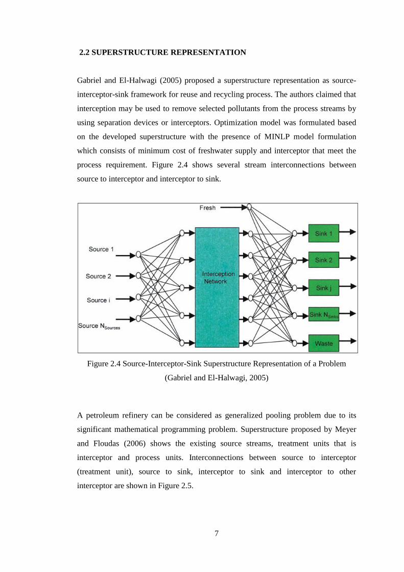
2.2 SUPERSTRUCTURE REPRESENTATION

Gabriel and El-Halwagi (2005) proposed a superstructure representation as source-

interceptor-sink framework for reuse and recycling process. The authors claimed that

interception may be used to remove selected pollutants from the process streams by

using separation devices or interceptors. Optimization model was formulated based

on the developed superstructure with the presence of MINLP model formulation

which consists of minimum cost of freshwater supply and interceptor that meet the

process requirement. Figure 2.4 shows several stream interconnections between

source to interceptor and interceptor to sink.

Figure 2.4 Source-Interceptor-Sink Superstructure Representation of a Problem

(Gabriel and El-Halwagi, 2005)

A petroleum refinery can be considered as generalized pooling problem due to its

significant mathematical programming problem. Superstructure proposed by Meyer

and Floudas (2006) shows the existing source streams, treatment units that is

interceptor and process units. Interconnections between source to interceptor

(treatment unit), source to sink, interceptor to sink and interceptor to other

interceptor are shown in Figure 2.5.

8

2.3 PARTITIONING REGENERATOR UNIT

Tan et al. (2009) discussed about integration of partitioning regenerator units in a

source-sink superstructure representation model. Partitioning regenerator unit can be

defined as splitting a contaminated water stream into a regenerated permeate stream

and a low-quality reject stream. This can be described in membrane separation-based

processes such as reverse osmosis (RO) and ultrafiltration. According to Tan et al.

(2009), both permeate and rich streams are potentially to be reused or recycle within

plant.

Several criteria are considered in formulation of the optimization model problem.

Some parts of the sources that have fixed flowrate and contaminant concentration

can be reused or recycled, flowed to regenerator (interceptor) or discharged to the

environment. On the other hand, there is a demand for specific flowrate of water at

below identified concentration maximum value for sinks. The mixed water produced

by different sources will be fed into a single partitioning regenerator unit where both

permeate and reject streams that discharged by the regenerator are potentially to be

reused or recycled within plant itself. An assumption is made on regenerator unit that

is fixed ratio of flowrates for permeate and rich streams and fixed contaminant

removal ratio.

Figure 2.5 Superstructure Representation for Generalized Pooling Problem

(Meyer and Floudas, 2006)

f 1 , 1

f 1 , 3

f 1 , 4

f 1 , 5

Source 2 f 1 , 2

Source 3

Source 4

Source 5

f 2 , 1

f 2 , 2 Sin

k 2

f 2 , 3

Source 1 TU 2

TU 1

TU 5

TU 4

TU 6

TU 3

Source flowrate f 1 , i and concentration c i Sink flowrate f 2 , j Source ( i ) Sink

Interceptor

Sink 1

Sink 3

9

2.4 PIECEWISE LINEAR RELAXATION

Relaxation involves outer-approximating the feasible region of a given problem and

underestimating (overestimating) the objective function of a minimization

(maximization) problem (Wicaksono and Karimi, 2008). It is achieved by applying

boundary on the complicating variables, that is for this case is bilinear variables, in

the original problem by means of under-, over- and/or outer-estimating the specific

variables. Based on the review done on several authors, it is shown that Piecewise

Linear Relaxation (PLR) is potentially can be a solution strategy in handling bilinear

variables in the optimization modelling problem.

Bilinear variable is a multiplication of two linear variables. Generally, it exhibits

multiple local optimal solutions and high degree of difficulty to locate its global

solution, especially for larger industrial scale problems. Due to its non-convexity,

there is no guarantee of global optimal solution that obtained from the potential local

solutions. As for water network design problems, bilinear variables are given by

multiplication of an unknown contaminant concentration term and an unknown

flowrate term in concentration balances which mostly occurs in concentration

balances.

Relaxation does not replace the whole original problem but offers guaranteed bounds

on the solutions of the problem. Bilinear enveloped proposed by McCormick (1976)

involves the substitution of additional variable, z into bilinear term, xy in the original

problem. The notion of relaxation includes the ab initio partitioning of search domain

and combining the continuous convex-to-convex relaxations based on convex

envelope of particular partitions into overall combined relaxation. The tightness of

overall discrete relaxation is improved due to convex relaxation of nonconvex

functions over smaller partitions of the feasible region.

Three ways in partitioning the search domain are big-M formulation, convex

combination formulation and incremental cost formulation. Computational

comparison of PLR had been conducted by Gounaris et al. (2009). It shows that Big-

M formulation always failed in obtaining the solutions for particular problem. On the

other hand, convex combination formulation provides major improvement but with

10

occurrence of failures in high-N regime only. In this work, incremental cost

formulation is chosen as the solution strategy due to the incremental nature of

problem. The comparison on solution strategy in handling bilinear variables is given

in Table 2.1.

11

Table 2.1 Comparison on Solution Strategy in Handling Bilinear Variables

Author Type of Model Solution Strategy to Handle Bilinear Variables Findings from Applying the Solution Strategy

Hasan and Karimi (in press) NA Piecewise Linear Relaxation (PLR)

Univariate and bivariate partitioning

Extensive numerical comparison between univariate

and bivariate partitioning

Gounaris et al. (in press) Pooling problem Piecewise Linear Relaxation (PLR)

Ab initio uniform (identical) univariate partitioning

using convex envelopes

Suitable for large-scale problems

Fast computational time

Pham et al. (2009) Pooling problem Piecewise Linear Relaxation

Discretization of quality variables

Suitable for large-scale problems

Fast computational time

Near-global optimal solution

Wicaksono and Karimi

(2008)

MILP on global mathematical

optimization problem Piecewise Linear Relaxation (PLR)

Univariate and bivariate partitioning

Improved relaxation quality with bivariate

partitioning

Solution time to obtain Piecewise Linear Relaxation

varies with MILP relaxation scheme

Saif et al. (2008) MINLP on reverse osmosis network

(RON) Convex relaxation on branch-and-bound algorithm

Piecewise underestimators and overestimators

Give very tight lower bound

Large solution time

Meyer and Floudas (2006)

MINLP on generalized pooling

problem for wastewater treatment

network

Augmented Reformulation–linearization technique

(RLT)

Smooth piecewise quadratic perturbation function

Piecewise discretization of quality variables

Give very tight lower bound

large solution time

Karuppiah and Grossmann

(2006)

Nonconvex GDP Integrated water

network systems

Piecewise Linear Relaxation (PLR) in branch-and-

bound algorithm

Branch-and-contract

Discretization of flow variables

Low solution time

Androulakis et al. (1995) NLP on general constrained

nonconvex problem Convex quadratic NLP relaxation named αββ

underestimator

Poor tightness of relaxation

Improved by Meyer and Floudas (2006) with smooth

piecewise quadratic perturbation function

Sherali and Alameddine

(1992) NA Reformulation–linearization technique (RLT) Longer computational time

McCormick (1976) Rectangle Convex and concave underestimators

Characterized as convex envelopes for bilinear terms

by Al-Khayyal and Falk

12

CHAPTER 3

METHODOLOGY

Figure 3.1 Methodology Chart

The method in this study starts with the understanding of the problem of water

network design for a petroleum refinery with the presence of water reuse,

regeneration and recycles (W3R) technique. Data for identified flowrates and

concentration of contaminants are collected from a refinery plant in Malacca. Then, a

superstructure representation is developed which includes all possible

interconnections between sources, a single interceptor that is reverse osmosis

network (RON), and sinks.

Understanding of water network design problem

Development of source-interceptor-sink superstructure representation

Formulation of MINLP optimization model

Application of solution strategy to handle bilinear variables and big-M logical constraints

Model implementation (GAMS) and optimal solution

Evaluation of the optimal solution

13

After that, the mixed-integer nonlinear programming (MINLP) optimization model is

formulated with the specified constraints and objective function which is to minimize

the usage of freshwater, wastewater discharged as well as the total cost for RON. The

model consists of bilinear variables that are the major problem in optimization model

which will be handled by Piecewise Linear Relaxation (PLR) as its solution strategy.

On the other hand, another problem occurs in optimization is Big-M logical

constraints which will be solved by specification of tighter upper and lower bound.

The next step involves the implementation of optimization model in General

Algebraic Modeling System (GAMS) modeling language to determine the feasible

optimal solution for the problem. GAMS modeling language software will be used for

this project. It is a high-level modeling system for mathematical programming and

optimization. It consists of a language compiler and a stable of integrated high-

performance solvers. GAMS is tailored for complex, large scale modeling

applications, and allows to build large maintainable models that can be adapted

quickly to new situation. Lastly, the solution will be evaluated based on the real-

world petroleum refinery practical features. The proposed key milestone for FYP II

is shown below.

Detail/Week 1 2 3 4 5 6 7 8 9 10 11 12 13 14

Research Progress

- Literature Review

- Objective Function

- Logical constraint formulation

- Revised formulation

Submission of Progress Report I

Research Progress

- Solution strategy

- Obtain optimal solution

Submission of Progress Report II

Pre-EDX

EDX

Submission of Final Report

Figure 3.2 Gantt Chart of FYP II

14

CHAPTER 4

OPTIMIZATION MODEL FORMULATION

4.1 SUPERSTRUCTURE REPRESENTATION

A superstructure is developed based on an actual operating refinery with multiple

sources, multiple interceptor units, and multiple sinks.

Interceptor

(RO)PERMEATE

REJECT

Source 1

Source 3

Source 2

Source n

Sink 1

Sink 3

Sink 2

Sink m

SOURCE TO SINK

SO

UR

CE

TO

IN

TE

RC

EP

TO

R

INTERCEPTOR TO SINK

INT

ER

CE

PT

OR

TO

SIN

K

Figure 4.1 Superstructure Representation of Possible Interconnections between

Source-Interceptor-Sink

The superstructure representation of source-interceptor-sink had been proposed

based on a local refinery plant water management as illustrated in Figure 4.1. The

problem representation is useful for developing material balances and other

constraints associated with the optimization model formulation. In this project, only

single stage reverse osmosis network is considered as the interceptor for the detailed

design parametric optimization, latter incorporates into the main optimization

15

problem. Figure 4.2 shows the general representation of source-interceptor-sink

structure.

InterceptorSQd (so,int)

QF,CF

Q1 (so)

Source 1

Source 2

Source n

Qb,perm (int,si)

Cb,perm

Qb,rej(int,si)

Cb,rej

Sink 1

Sink 2

Sink n

Q2 (si)Qa (so,si).

.

.

.

.

.

Figure 4.2 General Representation of Source-Interceptor-Sink

4.2 OPTIMIZATION MODEL FORMULATION

We consider two types of variables in our optimization model formulation that is

(1) continuous variables on the water flowrates and contaminant concentrations; and

(2) 0–1 variables (or binary variables) on the piping interconnections that involve

interconnections between the following entities:

between a source and a sink,

between a source and an interceptor,

between a permeate stream (of an interceptor) and a sink,

between a reject stream (of an interceptor) and a sink,

The binary variables are also employed to model the existences of the streams of an

interceptor, namely:

the inlet stream to an interceptor,

the outlet streams from an interceptor that comprises the concentrated reject

stream and the diluted permeate stream.

Material balances for the source-interceptor-sink superstructure representation are

developed for water flowrates and contaminant concentrations based on optimization

model formulations proposed by Tan et al. (2009), Meyer and Floudas (2006), and

Gabriel and El-Halwagi (2005). The identified values included are outlet flowrates of

sources, outlet concentrations of sources, inlet flowrate of sinks and maximum

16

allowable inlet concentration of sinks. Besides, liquid phase recovery, α and removal

ratio, RR are also considered for a single interceptor unit. The objective function and

material balances are described in the following sections.

4.2.1 Objective Function

The objective function of the problem is to minimize the overall cost which is

represented by the minimization of freshwater use and wastewater discharges, piping

interconnections cost, and reverse osmosis network cost (Ismail, 2010).

costmin obj cost of freshwater per year

+ cost of effluent treatment (discharge) per year

+ operating and capital cost of interceptor per year

+ operating and capital cost of pipelines per year

cost water

discharge

min obj load of freshwater AOT

+ load of discharge AOT

+ Total annualized cost of interceptor from detail design

operating cost parameter of pipeline load of the pipeli+

C

C

D

neAnnualizing Factor

capital cost parameter of pipeline existence of the pipeline

The complete objective function formulation is shown in equation (1).

cost water a discharge 2

si SI

Annualized cost of freshwater use and wastewater discharge treatment

co CO

Annualized cost of in

min obj freshwater,si (discharge) AOT

TAC CO

C Q C Q

terceptorfrom the parametric optimization problem in detailed design

dd

so SO int INT so SO int INT

b,perm

b,perm

int INT si SI so SO int INT

so,intso,int

3600

int,siint,si

3600

Qp q Y

v

Qp q Y

vD

b,rej

b,rej

int INT si SI so SO int INT

aa

so SO si SI so SO int INT

Annualized cost of operating

(1 )

(1 ) 1int,siint,si

3600

so,siso,si

3600

n

n

m m

mQp q Y

v

Qp q Y

v

and capital piping interconnections

(1)

17

4.2.2 Material Balances

4.2.2.1 Material Balances for Sources

Interceptor

Q1 (so)

Qd (so,int)

Sink 1

Sink 2

Sink m

Qa (so,si)

.

.

.

Source n

Figure 4.3 Representation of Material Balance for a Source

Figure 4.3 shows the flow representation of a source stream which can be splitted

into several streams for direct reuse to the sinks, and/or for regeneration (to the

interceptors) before the reuse. This representation is useful to develop the flow and

concentration balances for source.

(a) Flow balances for sources

1 d a

int INT si SI

so so,int so,si so SOQ Q Q

(2)

The flow balances for sources as given by (2) indicates that the flowrate of a source

Q1(so) is greater than the sum of the flowrate splits from the source to the interceptor

units for regeneration

d

int INT

so,intQ

and from the source to the sinks for direct

reuse or recycle a

si SINK

so,siQ

. The flow balance is applied to each source. It is

written as an inequality instead of an equality (as is typical of a flow balance) to

account for discharging any excess source of water directly into the environment

(Tan et al., 2009). It is noteworthy that if this flow balance is represented as equality,

the model is likely to return an infeasible solution.

18

(b) Concentration balances for sources

1 so so d so a

int INT si SI

so so,co so,co so,int so,co so,si

so SO, co CO

Q C C Q C Q

(3)

The concentration balance for a source (3) represents that the multiplication of the

contaminant concentration in the source stream Cso(so,co) with Q1(so) is equivalent

to the total of multiplication between Cso(so,co) and d

int INT

so,intQ

and

multiplication between Cso(so,co) and a

si SINK

so,siQ

.

Since Cso(so,co) in all terms can be canceled out, equation (3) is thereby equivalent

to equation (2), as shown below, thus equation (3) is negligible.

1 soso so,coQ C so so,coC d so

int INT

so,int so,coQ C

a

si SI

so,si

so SO, co CO

Q

1 d a

int INT si SI

so so,int so,si , so SOQ Q Q

4.2.2.2 Material Balances for Interceptors

InterceptorQd (so,int) Qb,perm (int,si)

Qb,rej (int,si)

Sink 1

Sink 2

Sink n

.

.

..

.

.

Source 1

Source 2

Source n

Figure 4.4 Representation of Material Balance for an Interceptor

Figure 4.4 shows the representation of an interceptor that receives the mixing of

source streams and generates the permeate and reject streams that are further splitted

19

to each sink. This representation is useful to develop the flow and concentration

balances for an interceptor.

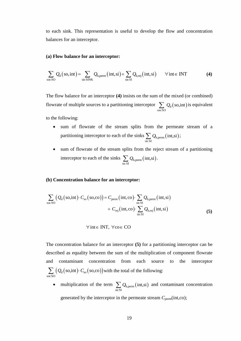
(a) Flow balance for an interceptor:

d b,perm b,rej

so SO si SINK si SI

so,int int,si int,si int INTQ Q Q

(4)

The flow balance for an interceptor (4) insists on the sum of the mixed (or combined)

flowrate of multiple sources to a partitioning interceptor d

so SO

so,intQ

is equivalent

to the following:

sum of flowrate of the stream splits from the permeate stream of a

partitioning interceptor to each of the sinks b,perm

si SI

int,siQ

;

sum of flowrate of the stream splits from the reject stream of a partitioning

interceptor to each of the sinks b,perm

si SI

int,siQ

.

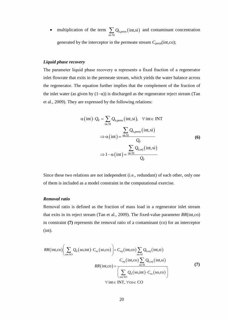
(b) Concentration balance for an interceptor:

d so perm b,perm

so SO si SI

rej b,rej

si SI

so,int so,co int,co int,si

int,co int,si

int INT, co CO

Q C C Q

C Q

(5)

The concentration balance for an interceptor (5) for a partitioning interceptor can be

described as equality between the sum of the multiplication of component flowrate

and contaminant concentration from each source to the interceptor

d so

so SO

so,int so,coQ C

with the total of the following:

multiplication of the term b,perm

si SI

int,siQ

and contaminant concentration

generated by the interceptor in the permeate stream Cperm(int,co);

20


si SI

int,siQ

and contaminant concentration

generated by the interceptor in the permeate stream Cperm(int,co);

Liquid phase recovery

The parameter liquid phase recovery α represents a fixed fraction of a regenerator

inlet flowrate that exits in the permeate stream, which yields the water balance across

the regenerator. The equation further implies that the complement of the fraction of

the inlet water (as given by (1α)) is discharged as the regenerator reject stream (Tan

et al., 2009). They are expressed by the following relations:

F b,perm

si SI

b,perm

si SI

F

b,rej

si SI

F

int int,si , int INT

int,si

int

int,si

1 int

Q Q

Q

Q

Q

Q

(6)

Since these two relations are not independent (i.e., redundant) of each other, only one

of them is included as a model constraint in the computational exercise.

Removal ratio

Removal ratio is defined as the fraction of mass load in a regenerator inlet stream

that exits in its reject stream (Tan et al., 2009). The fixed-value parameter RR(int,co)

in constraint (7) represents the removal ratio of a contaminant (co) for an interceptor

(int).

d so rej b,rej

so SO si SI

rej b,rej

si SI

d so

so SO

int,co so,int so,co int,co int,si

int,co int,si

int,co

so,int so,co

int INT, co CO

RR Q C C Q

C Q

RR

Q C

(7)

21

Alternatively, RR can be defined in terms of the parameters of the reject stream of an

interceptor as follows:

d so rej b,rej

so SO si SI

F F rej b,rej

si SI

rej b,rej

si SI

F F

int,co so,int so,co int,co int,si

int,co int,co int,co int,co int,si

int,co int,si

int,coint,co int,co

int INT, co CO

RR Q C C Q

RR Q C C Q

C Q

RRQ C

(8)

Accordingly, RR can be defined in terms of the parameters of the permeate stream of

an interceptor:

F F perm b,perm

si SI

F F

perm b,perm

si SI

F F

perm b,perm

si SI

F F

int,co int,co int,co int,si

int,coint,co int,co

int,co int,si

int,co 1int,co int,co

int,co int,si

1 int,coint,co int,co

int

Q C C Q

RRQ C

C Q

RRQ C

C Q

RRQ C

INT, co CONT

(9)

22

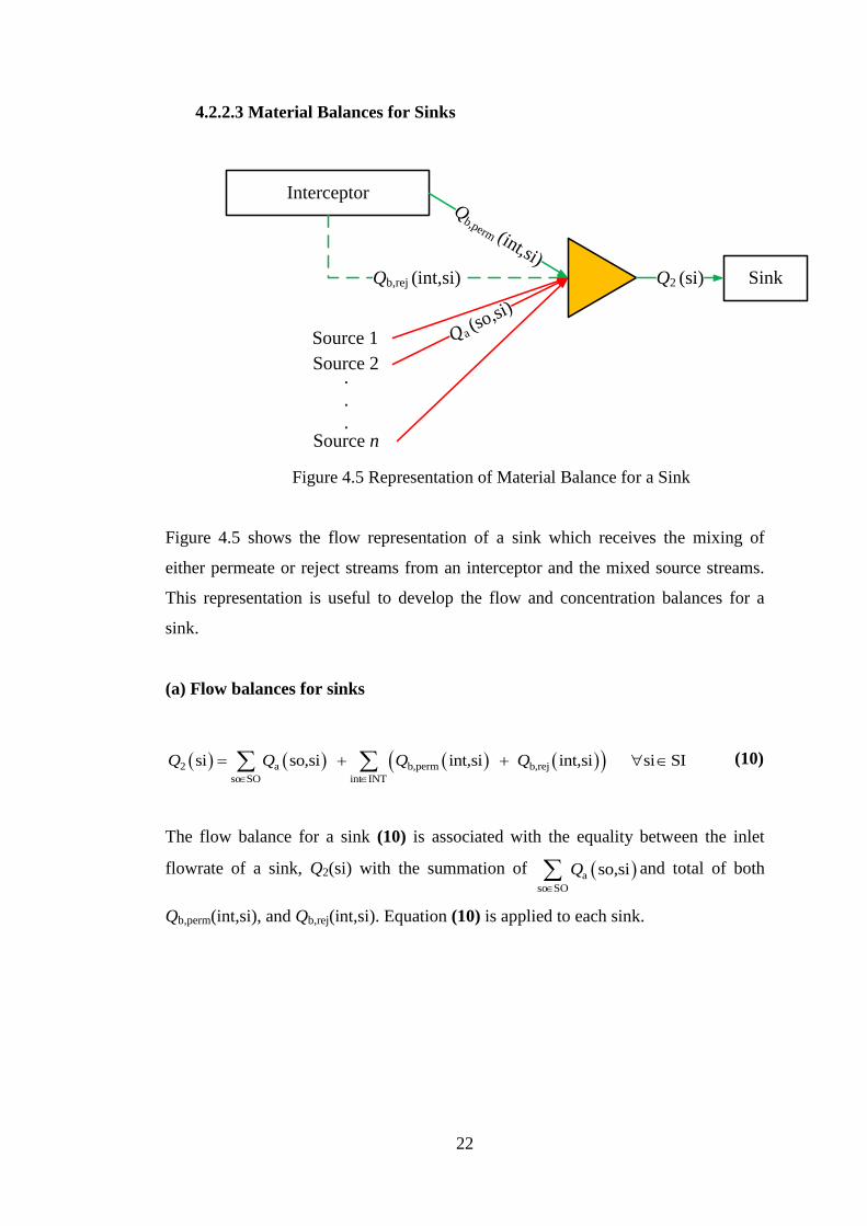
4.2.2.3 Material Balances for Sinks

Interceptor

Sink

Qb,perm (int,si)

Qb,rej (int,si)

Qa (so,si)

Source 1

Source 2

Source n

Q2 (si)

.

.

.

Figure 4.5 Representation of Material Balance for a Sink

Figure 4.5 shows the flow representation of a sink which receives the mixing of

either permeate or reject streams from an interceptor and the mixed source streams.

This representation is useful to develop the flow and concentration balances for a

sink.

(a) Flow balances for sinks

2 a b,perm b,rej

so SO int INT

si so,si int,si int,si si SIQ Q Q Q

(10)

The flow balance for a sink (10) is associated with the equality between the inlet

flowrate of a sink, Q2(si) with the summation of a

so SO

so,siQ

and total of both

Qb,perm(int,si), and Qb,rej(int,si). Equation (10) is applied to each sink.

23

(b) Concentration balances for sinks

a so perm b,perm rej b,rej

so SO int INT

2

so,si so,co int,co int,si int,co int,si

si si,co

si SI, co CO

Q C C Q C Q

Q C

(11)

The concentration balance for a sink (11) is depicted as above, where the summation

of a so

so SO

so,si so,coQ C

and perm b,perm rej b,rej

int INT

int,co int,si int,co int,siC Q C Q

is equivalent to multiplication of Q2(si) and the contaminant concentration into the

sink C(si,co).

Since there are specific values for maximum allowable contaminant concentration to

each sink, the term C(si,co) is changed to Cmax (si,co) and the inequality is taking

place. The term Q2(si) in equation (11) can be replaced by the equation (10). The

final formulation derivation of concentration balance for a sink is shown in equation

(12).

a so perm b,perm rej b,rej

so SO

a b,perm b,rej max

so SO int INT

so,si so,co int,co int,si int,co int,si

so,si int,si int,si si,co

si SI, co CO

Q C C Q C Q

Q Q Q C

(12)

(c) Restrictions on mixing of permeate and reject streams in sinks

The previous flow and concentration balances for a sink allow mixing of the

permeate and reject streams of a membrane-based interceptor at the inlet of a sink.

However, we ought to forbid such a mixing because the function of this type of

interceptor is to separate (or partition) its outlets into a concentrated stream (i.e., the

24

reject stream) and a diluted stream (permeate stream) before entering the sinks. This

constraint (13) is applicable to each sink as follows:

perm rejint,si int,si 1, si SI, int INTY Y (13)

The forbidden mixing constraint specifies that for a sink operation, only one of either

the permeate stream or the reject stream from each interceptor is allowed to enter the

sink.

The less-than-or-equal-to inequality allows none of the piping interconnections from

either a permeate or a reject stream to a sink to be selected for minimizing the

objective function value. In other words, the optimizer is susceptible to not selecting

any of the permeate and reject streams because the cost-minimization objective

function would tend to select as few piping interconnections (as modeled by 0–1

variables) as possible. But a solution without the presence of the outlet streams of an

interceptor would not be reasonable, hence we reformulate this constraint in the form

of an equality, as follows:

perm rejint,si int,si 1, si SI, int INTY Y (14)

The final form of this constraint ensures that at least one of either the permeate or the

reject stream is selected. But note that the constraint does not ensure that at least one

of the piping interconnections involving a permeate stream and at least one such

piping interconnection for a reject stream must be selected. This might not be a

concern because if the reject stream concentration of an interceptor is lower than the

maximum allowable concentration (or Cmax value) of a sink, then the reject stream

can be sent to the sink, and the corresponding permeate stream of that interceptor can

also be accepted into the sink, thus ensuring that both the permeate and reject streams

of an interceptor are selected.

25

4.2.3 Revised Formulation on Material Balances for Interceptors to Reduce

Bilinearities

InterceptorQperm(int)

Cperm(int)

Qrej(int)

Crej(int)

SsiQb,perm(int,si)

Cb,perm(int,si)

SsiQb,rej(int,si)

Cb,rej(int,si)

Sink 2

Sink m

.

.

.

Qd (so,int)

.

.

.

Source 2

Source 1

Source n

Sink 1QF

CF

Figure 4.6 Revised Subsuperstructure Representation of Interceptors

Figure 4.6 shows the revised subsuperstructure representation of an interceptor that

receives the mixing of source streams and generates the permeate and reject streams

that are further splitted to each sink. This representation is useful to develop flow and

concentration balances before the interceptors, for the interceptors and after the

interceptors.

(a) Flow balances for mixers before interceptors

d F

so SO

so,int , int INTQ Q

(15)

The flow balances for mixers before interceptors (15) enforces that the mixed or

combined flowrate of multiple sources to a partitioning interceptor d

so SO

so,intQ

is

equivalent to the feed flowrate to the interceptor QF.

(b) Concentration balances for mixers before interceptors

d so F F

so SO

so,int so,co int,co int,co , int INT, co COQ C Q C

(16)

The concentration balances for mixers before interceptors (16) for a partitioning

interceptor can be described as the equality between the multiplication

26

d so

so SO

so,int so,coQ C

with multiplication of QF(int,co) and contaminant

concentration of feed to the interceptor CF(int,co).

Note the following simple analysis to determine the number of bilinear terms:

knownparameter

d so F F

so SO1 bilinear term

no bilinear term

so,int so,co int,co int,co , int INT, co COQ C Q C

(c) Flow balances for interceptors

F perm rejint int , int INTQ Q Q (17)

The flow balance for interceptor (17) represents FQ is equivalent to the summation

of flowrate of permeate stream of a partitioning interceptor Qperm(int) and flowrate of

reject stream of a partitioning interceptor Qrej(int).

(d) Concentration balances for interceptors

F F perm perm rej rejint,co int int,co int int,co , int INTQ C Q C Q C

(18)

The concentration balance for interceptor (18) corresponds to the term F F int,coQ C

which is equivalent to the summation of multiplication between the term Qperm(int)

with contaminant concentration generated in the permeate stream Cperm(int,co) and

multiplication between the term Qrej(int) with contaminant concentration generated in

the reject stream Crej(int,co). However, the relations in equation (16) and (17) are

replaced into equation (18) and solved for Crej (19).

27

F F perm perm

rej

rej

F int F F

F

F

1

1

Q C Q CC

Q

Q C Q RR C

Q

Q

F FC Q

F

in

1

1

RR C

F

F

F

F

1 1

1

1

1

1

1 1

1

1

C RR

RRC

RR C

1

F

rej F

1

11

RR C

C RR C

(19)

At inlet to an interceptor, consider the following revised formulation of bilinear

concentration balances for interceptors, in which, we utilize the variable QF and CF.

known

d so F F

so SO1 bilinear term

no bilinear term

so,int so,co int,co int,co

int INT, co CO

Q C Q C

(20)

Concentration balance at the outlet of an interceptor is modeled after that of a splitter

concentration balance, which does not involve any bilinear term, as follows:

F b,perm1 int,co int,co int,co

int INT, co CO

RR C C

(21)

F b,rej1 int,co int,co

1

int INT, co CO

RR C C

(22)

28

Thus, this alternative formulation of concentration balances for interceptor (21) and

(22) only involves one bilinear term.

Nevertheless, note that equation (22) utilizes a different relation for the removal ratio

physical parameter as given by

rej F11

C RR C

. This relation holds true

even for the case of RR(int,co) = 0, in which an interceptor does not remove a certain

contaminant.

(e) Flow balances for splitters after interceptors

perm b,perm

si SI

int = int,si , int INTQ Q

(23)

The flow balance of permeate stream for splitter after interceptor is represented by

equation (23) where Qperm(int) equals to total flowrate for the stream splits from the

permeate stream of a partitioning interceptor to each of the sinks b,perm

si SI

int,siQ

.

rej b,rej

si SI

int int,si , int INTQ Q

(24)

The flow balance of reject stream for splitter after interceptor is represented by

equation (24) where Qrej(int) equals to total flowrate for the stream splits from the

reject stream of a partitioning interceptor to each of the sinks b,rej

si SI

int,siQ

.

(f) Concentration balances for splitters after interceptors

perm perm b,perm b,perm

si SI

int int,co = int,si int,co , int INTQ C Q C

(25)

The concentration balance of permeate stream for splitter after interceptor is

indicated by equation (25) where multiplication of Qperm(int) with contaminant

29

concentration generated in the permeate stream Cperm(int,co) is equivalent to


si SI

int,siQ

and Cperm(int,co).

rej rej b,rej b,rej

si SI

int int,co = int,si int,co , int INTQ C Q C

(26)

The concentration balance of reject stream for splitter after interceptor is indicated by

equation (26) where multiplication of Qrej(int) with contaminant concentration

generated in the reject stream Crej(int,co) is equivalent to multiplication of the term

b,rej

si SI

int,siQ

and Crej(int,co).

4.2.4 Detailed Design of Interceptor Model Formulation

The model formulation of RO detailed design that serves as offline parametric

optimization problem is based on El-Halwagi (1997). Such single-stage RON

synthesis problem can be described in Figure 4.7.

Reverse Osmosis Network Reject

Feed

d

so SO

F

F

so,int

int,co

(co)

Q

C

P

Permeate

b,rej

si SI

rej

R

int,si

int,co

Q

C

P

b,perm

si SI

perm

P

int,si

int,co

Q

C

P

Figure 4.7 Reverse Osmosis Network Synthesis Problem (El-Halwagi, 1997)

We consider the detailed design of a single-stage hollow fiber reverse osmosis

(HFRO) type module as our case study. We assume that the RON consists of three

(3) different types of unit operations (Saif et al., 2008):

1. pump to increase the pressure of the source streams;

2. RO modules that separate the feed into a concentrated stream (i.e., the

reject stream) and a diluted stream (permeate stream);

3. turbine to recover kinetic energy from high-pressure stream.

30

Equation (27) shows the derivation for total annualized cost (TAC) of the single-

stage RON consisting of the fixed costs for RO modules, pump, and turbine, and the

operating costs for pump and pretreatment chemicals. The TAC also considers the

operating value of turbine, as represented by the subtraction term in the function.

TAC Annualized fixed cost of modules Annualized fixed cost of pump

+ Annualized fixed cost of turbine + Annual operating cost of pump

Annual operating cost of pre-treatment chemicals

- Operating value

of turbine

Mathematically, the expression of the TAC function for HFRO is shown below.

module pump

electricity

turbine

pump

chemicals

electricity

TAC no of modules inlet load of pump

inlet load of pumpinlet load of turbine

amount of chemicals needed

inlet load of turbine

C C

CC

C

C

turbine

b,perm0.65si SI

module pump

P

0.43

turbine

electricity

pump

d chemicals turbine

so SO

RO,si

TAC power of pump

power of turbine

power of pumpAOT

so,RO AOT power of turbine

Q

C Cq

C

C

Q C

electricity AOTC

(27)

where

rejshell FP F P

F

5d F atm

so SO

5b,rej R atm

si SI

RO,coP1 , El-Halwagi, 1997

2 2 RO,co

power of pump so,RO 1.01325 10 , and

power of turbine RO,si 1.01325 10 .

m

Cq S A P P

C

Q P P

Q P P

31

Reformulation of total annualized cost of reverse osmosis network to eliminate

dependence on the type of contaminants

El-Halwagi (1997) defines the osmotic pressure of the RO at the feed side F as a

constant. Since the contaminant concentration of the permeate is very much lower

than that on the feed side, the osmotic pressure of the RO at the permeate side can be

neglected. Hence, to obtain a more detailed model that covers the representative

range encountered in the optimization procedure, the following relation is adopted, as

proposed by Saif et al. (2008), for the osmotic pressure at the reject side RO:

RO F,average

co

OS RO,coC (28)

where OS is a proportionality constant between the osmotic pressure and average

solute concentration on the feed side (Saif et al., 2008) whose value is in the range

between 0.006 to 0.011 psi/(mg/L) based on Parekh (1988). CF,average(RO,co) is the

average concentration for a contaminant (co) on the feed side, which is rewritten in

terms of the contaminant concentration on the permeate side as follows:

perm RO

coF,average

co

RO,co

RO,coc

C A P

CK

(29)

Where

Kc = the solute or contaminants permeability coefficient (1.82 108

m/s)

shellF P

P

2P P P

.

Hence, the relation for RO becomes:

perm RO

coRO

OS RO,co

c

C A P

K

(30)

32

Saif et al. (2008) proposed that the relation for the permeate flowrate from RO as:

P ROno of modules mQ A S P

Therefore,

P P

P RO

no of modulesm

Q Q

q A S P

(31)

Substituting RO and ∆P into the above relation gives:

b,perm b,perm

si SI si SI

P perm RO

co

b,perm

si SI

shellperm F P RO

coshellF P

RO,si RO,si

OS RO,co

'RO',si

POS RO,co

2P

2

m

c

m

c

Q Q

q C A P

A S PK

Q

C A P P

A S P PK

(32)

The final derivation of TAC from (27) until (32) is represented as (33):

33

b,perm

si SImodule

shellperm F P RO

coshellF P

annualized f

1 hRO,si

3600 sTAC

POS RO,co

2

2m

c

Q

C

C A P PP

A S P PK

ixed cost of module

0.65

5pump d F atm

so SO

annualized fixed cost of pump

tu

1 hso,RO 1.01325 10

3600 sC Q P P

C

R

0.43

5rbine b,rej F shell atm

si SI

annualized fixed cost of turbine

d

1 hRO,si 1.01325 10

3600 s

1 hso,

3600 s

P

Q P P P

Q

5F atm electricity

so SO

3pump

annual operating cost of pump

d chemicals

so SO

annua

RO 1.01325 10 AOT

W10

kW

1 hso,RO AOT

3600 s

P P C

Q C

R

l operating costof chemicals

5b,rej F shell atm turbine electricity

si SI

3

Operating va

1 hRO,si 1.01325 10 AOT

3600 s

W10

kW

P

Q P P P C

lue of turbine

co CO

(33)

The constraint on RO operating condition as associated with the feed pressure PF in

(33) is then given by:

F F shell shellF RP P F P

shellF P

2 2 2

2

P P P PP PP P P P P

PP P P

(34)

where

34

water FS

F

solutewater

perm

2solute S

, RO,co

, RO,co

, and M

NP C

A C

NN

C

DN C

K

while we adopt the following relation for CS in order to express PF in terms of

CF(RO,co) and Cperm(RO,co) (for the purpose of writing clarity, the indices have

been omitted here):

F R

P F

2S

C CC

Q C

RQ F RC Q R P FC Q C

R2 Q

P R F R R P F

R

F F R R P F

R

F F F F P P P F

R

F F P P P F

F P

2

2

2

2

2S

Q Q C Q C Q C

Q

Q C Q C Q C

Q

Q C Q C Q C Q C

Q

Q C Q C Q CC

Q Q

However, the above relation for CS contains bilinearities, hence we propose to utilize

the following alternative expression for CS:

F rej

S

F,RO,co rej

S

RO,co RO,co

2

RO,co

2

C CC

C CC

which yields:

35

F F P P P F F F F P P P F shell2

F P

P F P F F P

F d perm b,perm F b,perm

so SO si SI si SIF

perm d b,perm

so SO si SI

F F d

so SO

2 2" "

2 2C 2

21

SFC

2

2

MQ C Q C Q C Q C Q C Q C PD

P PK C A Q Q Q Q

C Q C Q C Q

PA

C Q Q

C Q

perm b,perm F b,perm

si SI si SI

F d b,perm

so SO si SI

shellP

2

2

C Q C Q

C Q Q

PP

where

F d

so SO

P b,perm

si SI

P perm

Q Q

Q Q

C C

and 2SFC MD

K

is the salt flux constant.

Finally, PF is derived as (35) with the substitution of SC .

36

shellF P

water F shellS P

F

solute

P F shellS P

F

2S

P

FS

F

2

C RO,co 2

RO,co

C RO,co 2

RO,co

RO,coC RO,co

M

PP P P

N PC P

A

N

C PC P

A

DC

K

C

CA

shellP

2 F R F RF

P F

shellP

2

RO,co RO,co RO,co RO,co

2 RO,co C RO,co 2

2

M

PP

D C C C C

K A C

PP

(35)

Hence, equation (35) can be simplified as follows:

F R R shellF F P

P F

SFC RO,co RO,co RO,co11

RO,co 2 C RO,co 2

C C C PP P

A C

(36)

Constant γ in (12) to (21) is defined as:

o s

5 4

i

161

1.0133 10

A r LL

r

(37)

where

37

1/2

o

5 2

i i

16

1.0133 10

A r L

r r

4.2.5 Big-M Logical Constraints

Big-M logical constraints relate continuous variables to 0–1 binary variables. For

water network problem, it represents a stream flowrate to existence of stream or pipe

connection. This constraint ensures non-zero flowrate when stream is selected in

optimal solution or vice versa. For instance, a binary variable of 1 implies the

existence of a stream that indicates there is a flowrate to operate the stream. For the

case of dealing with such logic constraints that involve continuous variables as

corresponded to this work, the conversion of that logic into mixed-integer constraints

is applied by using the ―big-M‖ constraints (Biegler et al., 1997). The ―big-M‖

parameters associated with these constraints are denoted as the upper and lower

bounds for the related continuous variables. Formulations of big-M logical

constraints on flowrates balances for this problem are shown in equations (38) until

(45).

Qa (so,si) ≤ a (so,si)M Ya (so,si) (38)

Qb,perm (int,si) ≤ ( , )b, permM int si Yb,perm (int,si) (39)

Qb,rej (int,si) ≤ ( , )b,rejM int si Yb,rej (int,si) (40)

Qd (so,int) ≤ ( , )dM so int Yd (so,int) (41)

Qa (so,si) ≥ ( , )aM so si Ya (so,si) (42)

Qb,perm (int,si) ≥ , ( , )b permM int si Yb,perm (int,si) (43)

Qb,rej (int,si) ≥ , ( , )b rejM int si Yb,rej (int,si) (44)

Qd (so,int) ≥ dM (so,int)Yd (so,int) (45)

tanh

2

2

1tanh

1

e e e

e e e

38

From the computational experiments, the lower bound for big-M constraints and

larger values of upper bound for big-M tend to give a poorer relaxation during

solution phase which leads to infeasible solution. Thus, specifications of tighter

lower and upper bounds for big-M constraints are required in order to solve this

problem.

Table 4.1 Specification on Upper Bound of Big-M Logical Constraints

Origin Destination Upper bound

Source Sink The smaller (minimum)

value between the two

Source Interceptor Follows source flowrate

Interceptor Sink Follows sink flowrate

Source and interceptor Discharge Summation of all sources

4.2.6 Model Tightening Constraints

The following constraints are enforced in the MINLP model for a complete

representation of the problem:

a) Lower and upper bounds on the variable flowrate of feed, QF(int) into the RO

interceptor

L UF F F(int) (int) (int)Q Q Q (46)

where

F d

so SO

(int) so,int int INTQ Q

In the computational experiments on the TAC minimization problem for offline

parametric optimization, the variable QF(int) into the RO interceptor tends to

assume the specified lower bound value. Therefore, a good lower bound value

has to be chosen for this purpose.

39

b) Lower and upper bounds on variable pressure of feed, PF into RO interceptor

L UF F FP P P (47)

It is noteworthy that equation (29) tends to give numerical difficulties in the

computational experiment arising from division with a zero value. Although this

can be overcome by specifying a non-zero lower bound value of Qb,perm, the

model solution still tends to be infeasible. Therefore, the lower and upper bound

values of variable PF are enforced in the model based on the common range

specified by El-Halwagi (1997).

c) Lower and upper bounds on variable osmotic pressure of RO interceptor, RO

at the reject side

L URO RO RO

(48)

The osmotic pressure tends to return as an illogical value (more than 1000 atm)

as the model is solved without specifying the upper and lower bounds on the

osmotic pressure. Therefore, both the upper and lower bound values have to be

incorporated into the model. However, it is also observed that the variable RO

tends to assume the specified upper bound value as they are incorporated. A

good upper bound value has to be chosen for this purpose.

d) Forbidden interconnection between the freshwater stream to RO interceptor

1 a

si SINK

'freshwater' 'freshwater',siQ Q

(49)

To avoid the freshwater from going directly into the RO interceptor, the above

constraint (49) is enforced so that the freshwater will only directly consumed by

the sinks. The contaminant concentrations in the freshwater shall be low enough

where the treatment of freshwater is not practical.

40

4.2.7 Solution Strategy in Handling Bilinearities by Piecewise Linear

Relaxation

A possible relaxation of bilinear variables would be to substitute every occurrence of

these variables by a new variable, z. They are restricted by adding the following

linear constraints:

convex envelope:

(a)

(b)

concave envelope:

(a)

(b)

L L L L

U U U U

U L L U

z y x x y x y

z y x x y x y

z y x x y x y

z

L U U Ly x x y x y

(50)

where in this case, variable flowrate,Q is represented by x while variable

contaminant concentration,C is indicated by y.

Applying the incremental cost formulation to model partitioning the search domain,

the use of (n) as binary variables is occupied.

1, if

( ) mu , 1 10, otherwise

x x nn n rr n N

(51)

First, we use the local incremental variable in (3)

1

( ) ( ) 0 ( ) 1

where

( ) ( )

( ) ( 1)

NL

n

Q Q d n u n u n

u n n

u n n

(52)

Note that the following constraints are added in each partition (Wicaksono and

Karimi, 2008)

(1) (1)

( ) ( 1)

u

u n n

(53)

41

Next, multiplying (52) by δC and defining δw(n) = δu(n) δy where δC = C-CL give

us:

1

L L L L

1

L L L L L

1( )

L L L L

1

( ) ( )

( ) ( )

( ) ( )

( ) ( )

NL

n

N

n

N

nzw n

N

n

Q C Q C C d n u n

Q C C Q C C C C d n u n

QC QC Q C Q C d n u n C C

z QC Q C Q C d n w n

(54)

The hard bounds of δu(n) is taken into consideration compared to the tighter bounds

of δu(n) which involves the variable θ. The convex and concave envelope can be

tighten up by replacing the following relations into (50).

L

L

U

L

U U L

( )

0

1

0

z QC

Q u n

C C C

Q

Q

C

C C C

The derivations are represented by (55) – (58).

L

L

convex envelope (a):

0 ( ) 0 ( ) 0 0

( ) ( ) 0

( ) 0 (eliminated)

L L L Lz C Q Q C Q C

QC u n C C

u n C C

w n

(55)

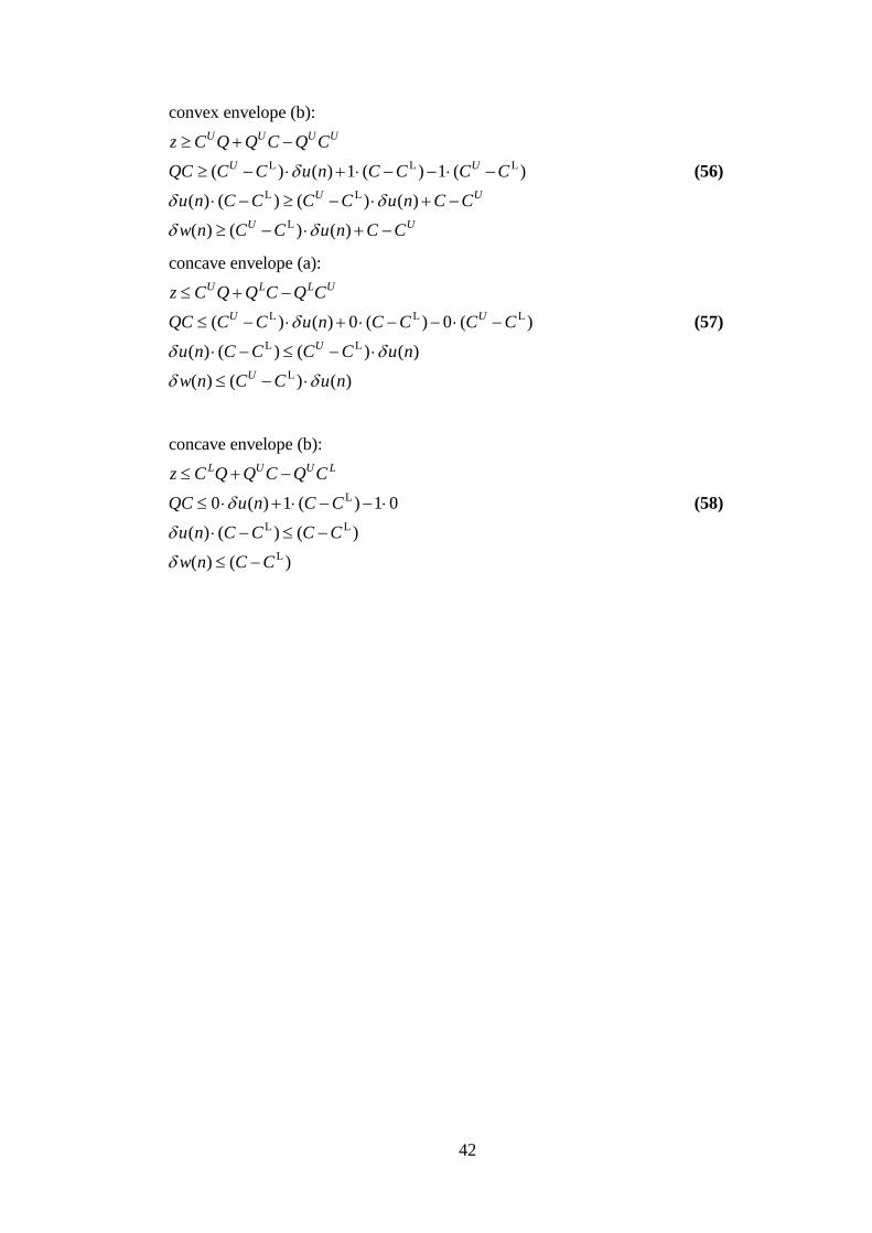
42

L L L

L L

L

convex envelope (b):

( ) ( ) 1 ( ) 1 ( )

( ) ( ) ( ) ( )

( ) ( ) ( )

U U U U

U U

U U

U U

z C Q Q C Q C

QC C C u n C C C C

u n C C C C u n C C

w n C C u n C C

(56)

L L L

L L

L

concave envelope (a):

( ) ( ) 0 ( ) 0 ( )

( ) ( ) ( ) ( )

( ) ( ) ( )

U L L U

U U

U

U

z C Q Q C Q C

QC C C u n C C C C

u n C C C C u n

w n C C u n

(57)

L

L L

L

concave envelope (b):

0 ( ) 1 ( ) 1 0

( ) ( ) ( )

( ) ( )

L U U Lz C Q Q C Q C

QC u n C C

u n C C C C

w n C C

(58)

43

CHAPTER 5

RESULTS AND DISCUSSION

5.1 PROBLEM DATA FOR MODEL

Table 5.1 Fixed Flowrates for Sources Source Flowrate (m

3/h)

PSR-1_ProcessArea 23

BW1 1.8

BD3 3.5

OWe-RG2 25

BDBLs2 72.3

SW2 2

Table 5.2 Fixed Flowrates for Sinks Sink Flowrate (m

3/h)

FIREWATER 3

OSW-SB 144

BOILER 128.3

HPU2 29.7

PSR1_SW 2

BDBLu 56.3333

Table 5.3 Maximum Inlet Concentration to the Sources Source Maximum Allowable Inlet Concentration for TSS (mg/L)

PSR-1_ProcessArea 40

BW1 37

BD3 1.00

OWe-RG2 12

BDBLs2 0.129

SW2 10

FRESHWATER 300

Note: Standard B Limit 100

Table 5.4 Maximum Inlet Concentration to the Sinks Sink Maximum Allowable Inlet Concentration for TSS (mg/L)

FIREWATER 25

OSW-SB 20

BOILER 20

HPU2 25

PSR1_SW 25

BDBLu 25

Discharge 100

Note: Standard B Limit 100

Table 5.5 Liquid Phase Recovery α and Removal Ratio RR for Reverse Osmosis

Interceptor Parameters Fixed Values

Liquid Phase Recovery, α 0.7

Removal Ratio of TSS Contaminant 0.975

44

Table 5.6 Economic Data, Physical Constants, and Other Model Parameters (mainly

for objective function formulation) Parameters Fixed Values

Annual operating time, AOT 8760 hr/yr

Unit cost for discharge (effluent treatment), Cdischarge $0.22/ton

Unit cost for freshwater, Cwater $0.13/ton

Manhattan distance, D 100 m

Fractional interest rate per year, m 5% = 0.05

Number of years, n 5 years

Parameter for piping cost based on CE plant index, p 7200 (carbon steel piping at CE plant index = 318.3)

Parameter for piping cost based on CE plant index, q 250 (carbon steel piping at CE plant index = 318.3)

Velocity, v 1 m/s

Table 5.7 Economic Data for Detailed Design of HFRO Interceptor Parameters Fixed Values

Viscosity of water µ 0.001 kg/m.s

Water permeability coefficient, A 5.573 × 10-8

m/s.atm

Annual operating time, AOT 8760 hr/yr

Cost of pretreatment chemicals, Cchemicals $0.03/m3

Cost of electricity, Celectricity $0.06/kW.hr

Cost per module of HFRO membrane, Cmodule $2300/yr.module

Cost coefficient for pump, Cpump $6.5/yr.W0.65

Cost coefficient for turbine, Cturbine $18.4/yr.W0.43

Table 5.8 Geometrical Properties and Dimensions for Detailed Design of HFRO

Interceptor Module Property Value

Solute (contaminant) flux constant, D2M /Kδ 1.82 × 10-8

m/s

HFRO fiber length, L 0.750 m

HFRO seal length, Ls 0.075 m

Permeate pressure from interceptor, Pp 1 atm

Inside radius of HFRO fiber, ri 21 × 10-6

m

Outside radius of HFRO fiber, ro 42 × 10-6

m

Membrane area per module Sm 180 m2 per module

Table 5.9 Physical Properties for Detailed Design of HFRO Interceptor Module Property Value

Shell side pressure drop per HFRO membrane

module, ΔPshell 0.4 atm

Pump efficiency, ηpump 0.7

Turbine efficiency, ηturbine 0.7

Osmotic pressure coefficient at HFRO, OS 0.006 psi/(mg/L) = 4.0828× 10-4

atm

Solute (contaminant) permeability coefficient, KC 1.82 108

m/s

45

5.2 COMPUTATIONAL RESULTS

We consider four case studies that are simplified variants of an actual real-world

industrial-scale water network design problem to demonstrate the proposed model

formulation and modeling approach in general. The cases involve seven sources, one

interceptor of reverse osmosis treatment technology, seven sinks, and one quality

parameter of contaminant concentrations. The comparisons between these case

studies are illustrated below.

Table 5.10 Comparison between Case Study 1, 2, 3 and 4 Case Study Model Formulation Solution Strategy

Case Study 1 Conventional mass balances (Tan et al., 2009;

Meyer and Floudas, 2006; and Gabriel and El-

Halwagi, 2005)

Without PLR

Case Study 2 Revised formulation on material balances for

interceptors and on expression for CF

Without PLR

Case Study 3 Conventional mass balances Convex relaxation based on

PLR

Case Study 4 Revised formulation on material balances for

interceptors and on expression for CF

Convex relaxation based on

PLR

Table 5.11 Comparisons of Computational Results to Determine the Optimal Design

and Suitable Solution Strategies

No Item Case Study

1

Case Study

2

Case Study

3

Case Study

4

1 Economic parameters

a Total cost for water integration and retrofit

(dollar per year) 466 800 470 300 615 300 554 100

b Total annualized cost (TAC) of RO 96 290 96 290 96 290 18 850

2 Design parameters of RO

a Feed pressure into interceptor, PF (atm) 56.812 56.812 56.812 1.400

b Reject pressure from interceptor, PR (atm) 56.412 56.412 56.412 1.000

c Osmotic pressure at reject side, ΔπRO 55.000 32.500 10.000 21.250

d Optimal duties of RON

Power of pump (kW) 62 840 62 840 113 600 814.0

Power of turbine (kW) 18 720 18 720 445 600 0

3 Water flowrates

a Total freshwater with reuse, regeneration and

recycle (m3/hr)

243.033 241.033 285.736 253.262

b Total inlet flow into RO QF (m3/h) 40.000 40.000 40.000 40.000

c Total permeate stream outlet flow of RO QP

(m3/h)

28.000 28.000 39.900 28.000

d Total reject stream outlet flow of RO QR (m3/h) 12.000 12.000 0.100 12.000

4 Contaminant concentrations

a Feed concentration into RO interceptor

CF(RO,co) (mg/L) 0.129 0.129 0.0004 6.107

b Permeate concentration from RO interceptor

Cperm(RO,co) (mg/L) 0.005 0 0 0.153

c Reject concentration from RO interceptor

Crej(RO,co) (mg/L) 0.419 0.430 0 20.000

46

Note: All values are reported to the nearest 4 significant values. Any flowrate value smaller than 0.05

m3/h is taken to be zero (which indicate that the associated piping interconnection is not operated).

Table 5.12 Model Sizes and Computational Statistics

Case Study Case Study 1 Case Study 2 Case Study 3 Case Study 4

Type of model MINLP MINLP MINLP MINLP

Solver GAMS/BARON GAMS/BARON GAMS/BARON GAMS/BARON

No. of continuous variables 162 164 809 802

No. of discrete binary variables 70 70 87 87

No. of constraints 107 110 1027 1043

No. of iterations 0 0 0 0

CPU time (s) (resource usage) 3369.250 3592.940 15.760 19.840

Remarks Integer Solution Integer Solution Integer Solution Integer Solution

Figure 5.1 Comparison on Computational Time for 4 Case Studies

5.2.1 Calculation for percentage of reduction on computational time

Take average time (s) for case study without PLR and with PLR, we get:

3480 17Reduction (%) 100 99.51%

3480

0

500

1000

1500

2000

2500

3000

3500

4000

1 2 3 4

Computational Time

(s)

Case Study

47

5.2.2 Optimum Allocation of Source-Interceptor-Sink

1.8

25

SW2

PSR_1_ProcessArea 23

BW1

Owe_RG2

2

243.033FRESHWATER

72.3BDBLs2

SOURCES

INTERCEPTOR

3

144

29.7

2

56.333

FIREWATER

OSW–SB

BOILER

HPU2

BDBLu

128.3

SINKS

(40,0

)

3.5BD3

REVERSE

OSMOSIS

NETWORK

PERMEATE

(28, 0.005)

REJECT

(12, 0.419)

PSR1_SW

INLET RO

(40, 0.129)

(3.0, 0)

(12.0, 0)

(5.3, 0)

(17.7, 0)

(25.0, 0)(21.0, 0)

(11.3, 0)

(100.0, 0)

(98.0, 0)

(45.033, 0)

(23.0, 0)

(2.0

, 0)

Figure 5.2 Optimal Network Structure for Case Study 1

1.8

25

SW2


BW1

Owe_RG2

2

241.033FRESHWATER

72.3BDBLs2

SOURCES

INTERCEPTOR

3

144

29.7

2

56.333

FIREWATER

OSW–SB

BOILER

HPU2

BDBLu

128.3

SINK

(40,0

)

3.5BD3

REVERSE

OSMOSIS

NETWORK

PERMEATE

(28, 0)

REJECT

(12, 0.430)

PSR1_SW

INLET RO

(40, 0.129)

(11.3, 0)

(7.7, 0)

(2.0, 0)

(25.0, 0)(15.3, 0)

(3.0, 0)

(16.3, 0)

(13.0, 0)(100.0, 0)

(100.0, 0)

(41.033, 0)

(16.7

, 0)(12.0, 0)


1.8

25

SW2


BW1

Owe_RG2

2

285.736FRESHWATER

72.3BDBLs2

SOURCES

INTERCEPTOR

3

144

29.7

2

56.333

FIREWATER

OSW–SB

BOILER

HPU2

BDBLu

128.3

SINKS

(40, 0)

3.5BD3

REVERSE

OSMOSIS

NETWORK

PERMEATE

(39.9, 0)

REJECT

(0.1, 0)

PSR1_SW

INLET RO

(40, 0.0001)

(3.0, 0)

(9.703, 0)

(19.0, 0)

(18.597, 0)

(100.0, 0)

(100.0, 0)

(29.403, 0)

(56.333, 0)

(25.0, 0)

(0.297, 0)(2.0, 0)


48

1.8

25

SW2


BW1

Owe_RG2

2

285.736FRESHWATER

72.3BDBLs2

SOURCES

INTERCEPTOR

3

144

29.7

2

56.333

FIREWATER

OSW–SB

BOILER

HPU2

BDBLu

128.3

SINKS(15, 0

)

3.5BD3

REVERSE

OSMOSIS

NETWORK

PERMEATE

(28, 0.153)

REJECT

(12, 20)

PSR1_SW

INLET RO

(40,6.107)

(17.441, 0.153)(1.729, 0)

(26.559, 0)

20.496

25.245100

97.245

56.017

(25, 0)

(10.5

59, 0

.153)

1.271, 20

4.455, 202, 200.316, 20

3.958, 20

3.958 Discharge


Note: values in parentheses on stream lines indicate water flowrates in m

3/h, contaminant

concentration in mg/L

5.3 DISCUSSION

Based on the comparison of computational results for case study 1, 2, 3 and 4 that is

explained in previous section, it shows that the formulation with convex relaxation

based on Piecewise Linear Relaxation (PLR) gives a much lower computational time

which is proposed by Gounaris, Misener and Floudas (2009). The notion proposed

by Pham et al. (2009) is proven which stated that this solution strategy can give fast

computational time for a large-scale problem. The results demonstrated that PLR can

improve the results in terms of the tightness of lower bound in such a way the

original domain of one of the two variables in bilinear terms is partitioned into many

subdomains and the principles of bilinear relaxation are applied for each of them

(Gounaris et al., 2009).

The optimum structure of source-interceptor-sink for these case studies mostly

involves water regeneration-reused as its water minimization technique. Case Study

4 represents a better possible freshwater usage as well as the interconnections

between interceptor and the sinks since it supplies to more sinks compared to the

other case studies. Although Case Study 1 registers the lowest cost, this may not be

the global optimal solution. The formulation with reduced bilinearities in Case Study

49

4 represents a more attractive solution, which to some extent proves the benefit of

avoiding nonconvexities due to bilinearities.

The formulation with reduced bilinearities offers a more cost-effective design,

presents a better design that involves generally lower pressure and requires less

pumping power that leads to a lower cost. Besides, the formulation with reduced

bilinearities presents an optimal design that omits the use of turbine as a final energy

recovery stage because the reject stream is at a relatively low pressure.

In general, the formulation with reduced bilinearities proposes an optimal design that

is competitive against the designs presented by the other approaches. Despite

involving the highest concentrations, the formulation with reduced bilinearities is

still within the regulatory limits.

50

CHAPTER 6

CONCLUSION AND RECOMMENDATION

6.1 CONCLUSION

All in all, this work proves that Piecewise Linear Relaxation can give fast

computational time for a large-scale optimization problem. It can be applied as a

solution strategy in handling the bilinearities in this case. The revised formulation for

interceptor where the bilinear terms in this problem are reduced with the presence of

PLR technique proposes the best global optimal solution. The development of these

techniques and tools are significant in order to deal with the integrated water

management problem at petroleum refineries, which become the main concern and

interest associated with the shortage of freshwater supply within our country.

6.2 RECOMMENDATION

It is recommended to apply Piecewise Linear Relaxation in the actual real-world

industrial-scale water network design problem which is very much a larger problem

compared to the case studies. Besides, multiple contaminants can also be considered

along with the complex detailed design of other interception technologies model

formulation. Despite problem for a petroleum refinery, the application of PLR should

be explored in various problems such as for a chemical plant or heat integration

network problem.

51

REFERENCES

Androulakis, I. P., Maranas, C. D., and Floudas, C. A. (1995). : A Global

Optimization Method for General Constrained Nonconvex Problems. J. of

Global Optimization. 7, 337-363.

Biegler, L. T., Grossmann, I. E., and Westerberg, A. W. (1997). Systematic Methods

of Chemical Process Design. New Jersey: Prentice-Hall.

El-Halwagi, M. M. (1997). Pollution Prevention through Process Integration. San

Diego, California, USA: Academic Press.

Gabriel, F. B. and M. M. El-Halwagi. (2005). Simultaneous Synthesis of Waste

Interception and Material Reuse Networks: Problem Reformulation for

Global Optimization. Environmental Progress 24, 2, 171–180.

Gounaris, C. E., Misener, R., and Floudas, C. A. (2009). Computational Comparison

of Piecewise-Linear Relaxations for Pooling Problems. Industrial &

Engineering Chemistry Research , 48, 5742–5766.

Ismail, Norafidah. (2010). Optimization with integrated offline parametric

optimization of detailed process model of an interceptor unit for water

network synthesis and retrofit design. Undergraduate thesis. Tronoh,

Malaysia: Universiti Teknologi PETRONAS.

Karuppiah, R., and Grossmann, I. E. (2006). Global Optimization for the Synthesis

of Integrated Water Systems in Chemical Processes. Computers & Chemical

Engineering, 30(4), 650-673.

McCormick, G. P. (1976). Computability of global solutions to factorable nonconvex

programs—Part I—convex underestimating problems. Mathematical

Programming 10: 146–175.

52

Meyer, C. A., and Floudas, C. A. (2006). Global Optimization of a Combinatorially

Complex Generalized Pooling Problem. AIChE Journal , 52 (3), 1027-1037.

Pham, V., Laird, C., and El-Halwagi, M. (2009). Convex Hull Discretization

Approach to the Global Optimization of Pooling Problems. Industrial &

Engineering Chemistry Research , 48, 1973-1979.

Saif, Y., Elkamel, A., and Pritzker, M. (2008). Global Optimization of Reverse

Osmosis Network for Wastewater Treatment and Minimization. Ind. Eng.

Chem. Res. , 47, 3060-3070.

Saif, Y., Elkamel, A., and Pritzker, M. (2008). Optimal Design of Reverse-Osmosis

Networks for Wastewater Treatment. Chemical Engineering and Processing ,

47, 2163–2174.

Sherali H. D., and Alameddine A., (1992) A New Reformulation-Linearization

Technique for Bilinear Programming Problems. J. of Global Optimization. 2,

379.

Smith, R. (2005). Chemical Process : Design and Integration. England: John Wiley

& Sons.

Tan, R. R., Ng, D. K., Foo, D. C., and Aviso, K. B. (2009). A Superstructure Model

for the Synthesis of Single-Contaminant Water Networks with Partitioning

Regenerators. Process Safety and Environment Protection , 87 (3), 197-205.

Tjun, B. S. (2009). Optimization of Petroleum Refinery Water Network Retrofit with

Opportunities for Water Reuse, Recycle and Regeneration (W3R). B Hons

Thesis, University of Technology Petronas, Chemical Engineering

Department, Tronoh.

Wang, Y. P., and Smith, R. (1994). ‗Wastewater Minimization. Chemical

Engineering Science , 49 (7), 981-1006.

53

Wicaksono, D. S., and Karimi, I. A. (2008). Piecewise MILP Under- and

Overestimators for Global Optimization of Bilinear Programs. 54(4).

Optimization of Water Network Design for a Petroleum Refinery

Documents

Transcript of Optimization of Water Network Design for a Petroleum Refinery