OPTIMIZATION OF THE SVM REGULARIZATION PARAMETER C IN MATLAB

FOR THE OBJECT-BASED CLASSIFICATION OF HIGH VALUE CROPS USING

LIDAR DATA AND ORTHOPHOTO IN BUTUAN CITY, PHILIPPINES

Rudolph Joshua U. Candare1, Michelle V. Japitana

2, James Earl Cubillas

3, and Cherry Bryan Ramirez

4

1,2,3,4 Phil-LiDAR 2 Project, College of Engineering and Information Technology, Caraga State University

Email: rjcandare@gmail.com

KEY WORDS: OBIA, LiDAR, Support Vector Machine, Machine Learning, eCognition, Matlab

ABSTRACT: This paper describes the processing methods used for the detailed resource mapping of different high

value crops in Butuan City, Philippines. The proposed methodology utilizes object-based image analysis and the

use of optimal features from LiDAR data and Orthophoto. Classification of the image-objects was done by

developing rule sets in eCognition. LiDAR data was used to create a Normalized Digital Surface Model (nDSM)

and a LiDAR intensity layer. The nDSM and LiDAR intensity layers were then paired with Orthophotos and were

segmented using eCognition for feature extraction. Several features from the LiDAR data and Orthophotos were

used in the development of rulesets for classification. Generally, classes of objects can't be separated by simple

thresholds from different features making it difficult to develop a rule set. To address this problem, the image-

objects were subjected to a supervised learning algorithm. Among the machine learning algorithms, Support Vector

Machine learning has recently received a lot of attention and the number of works utilizing this technique continues

to increase. SVMs have gained popularity because of their ability to generalize well given a limited number of

training samples. However, SVMs also suffer from parameter assignment issues that can significantly affect the

classification results. More specifically, the regularization parameter C in linear SVM has to be optimized through

cross validation to increase the overall accuracy. After performing the segmentation in eCognition, the optimization

procedure as well as the extraction of the equations of the hyper-planes was done in Matlab. The optimization

process can be time-consuming. To resolve this, parallel computing is employed for the cross validation process

which significantly speeds up the process. The learned hyper-planes separating one class from another in the multi-

dimensional feature space can be thought of as super-features which were then used in developing the classifier rule

set in eCognition. In this study, we report an overall classification accuracy of around 95%. Seven features from the

segmented LiDAR nDSM and intensity layers were used; area, roundness, compactness, height, height standard

deviation, asymmetry and intensity. Eight features from the segmented Orthophotos were used; two features ( a*

and b*) from CIELAB color space, three features (x, y and z) from CIEXYZ color space, two features (first, and

second coordinate) from one-dimensional scalar constancy, and one feature called RGB Intensity. We also show the

different feature-space plots that have driven the proponents to use the aforementioned features for all the different

classes.

1. INTRODUCTION Recently, a new approach called OBIA- Object-based image analysis, has been gaining a large amount of attention

in the remote sensing community. When methods become contextual they allow for the utilization of “surrounding”

information and attributes. This increases the importance of ontologies - as compared to the per pixel analysis.

The OBIA workflows are highly customizable allowing for the presence of human semantics and hierarchical

networks (Blaschke, 2011). Generally, there are two main processes in OBIA, segmentation and classification.

Segmentation is the process wherein adjacent pixels are grouped together based on their homogeneity thereby

creating meaningful “objects”. These objects are then subjected to classification. Both segmentation and

classification can be done with ease through different algorithms in eCognition (eCognition Reference Book, 2014).

Object-based classification can be done through user-defined rule-sets. However, different classes of objects aren‟t

separable by direct thresholding one feature at a time. Hence, samples from different classes of objects need to be

classified using machine learning algorithms.

Among the machine learning algorithms, Support Vector Machine has recently received a lot of attention and the

number of works utilizing this technique has increased exponentially. Support Vector Machines can generalize well

given a limited number of training samples. The most important characteristic is SVM‟s ability to generalize well

from a limited amount and/or quality of training data. Compared to other methods like artificial neural networks,

SVMs can yield comparable accuracy using a much smaller training sample size. This is due to the „„support

vector‟‟ concept that relies only on a few data points to define the hyper-plane that best separates the classes

(Mountrakis et al., 2010). An added advantage is that there is no need for repeating classifier training using

different random initializations or architectures. Furthermore, being non-parametric, SVMs do not assume a known

statistical distribution of the data to be classified. This is very useful because the data acquired from remotely

sensed imagery usually have unknown distributions. This allows SVMs to outperform techniques based on

maximum likelihood classification because normality does not always give a correct assumption of the actual pixels

distribution in each class (Su et al., 2009). The method is presented with a set of labelled data instances (the sample

objects) and the SVM training algorithm finds a hyper-plane that separates the dataset into a discrete predefined

number of classes that are consistent with the training samples (Vapnik, 1979). The term “hyper-plane” is used to

refer to the decision boundary that minimizes misclassifications, obtained in the training step. Learning is the

iterative process of finding a classifier with optimal decision boundary to separate the training patterns (Zhu and

Blumberg, 2002).

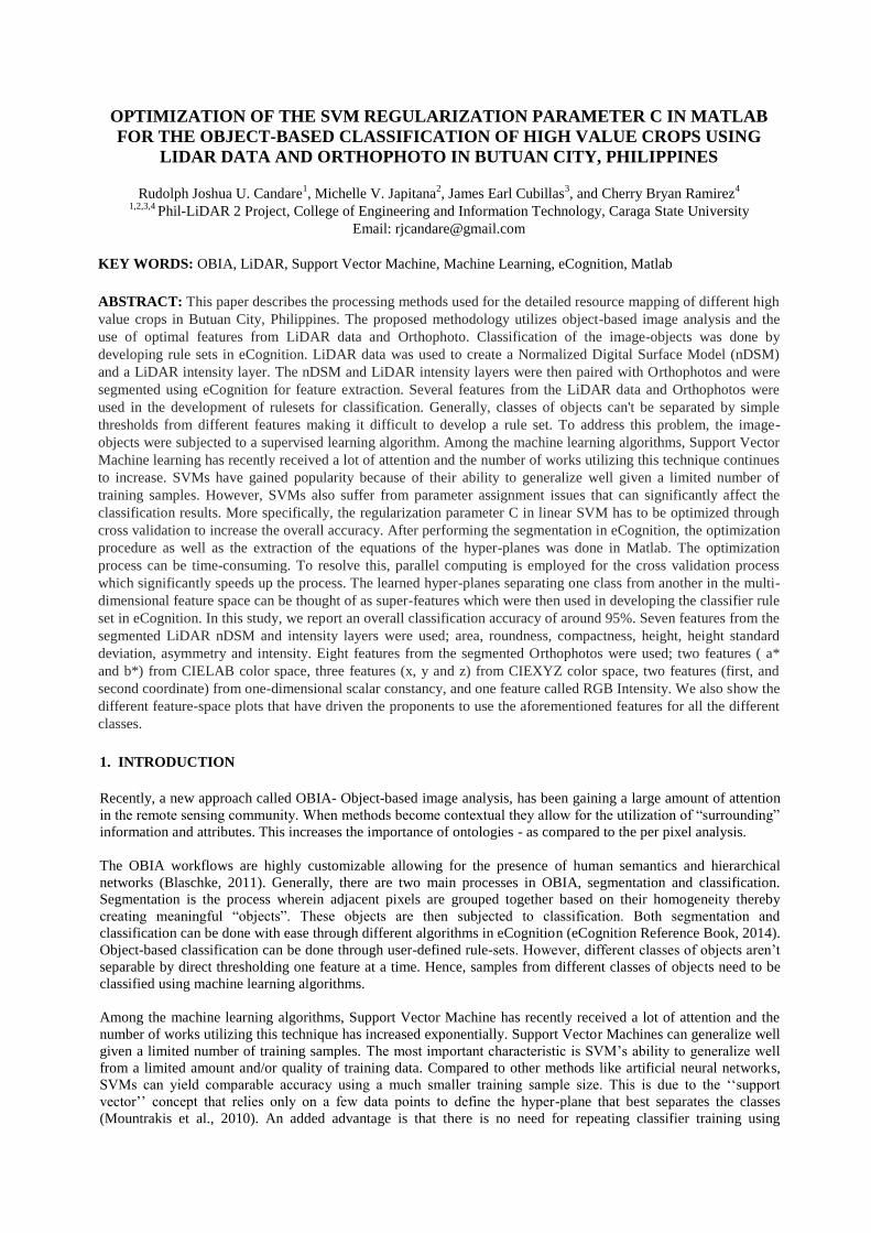
Figure 1. SVM hyper-plane dividing the Sample instances (objects). Adapted from (Burges, 1998)

The one-against-one formulation of the SVM constructs k(k-1)/2 classifiers (k is the total number of classes) where

each one is trained on data from two classes. For training data from the ith and the jth classes, we solve the

following binary classification problem:

( ) ∑ (1)

( ) ( ) (2)

( ) ( ) (3)

(4)

Minimizing

w

Tw means that we would like to maximize

‖ ‖, the margin between each groups of data. When data

are not linear separable, there is a penalty term ∑ which can reduce the number of training errors. The basic

concept behind SVM is to search for a balance between the regularization term and the training errors (Chih-Jen

Lin, 2001). After the classifiers have been constructed, an instance would be classified based on its sign with

respect to the hyper-plane. For example, if sign((wij)

Txi + b

ij) >0 then xi is in the ith class. Choice of the parameter

value (usually denoted by C), which controls the trade-off between maximizing the margin and minimizing the

training error, is also an important consideration in SVM application. There exists no established heuristics for

selection of these SVM parameters which frequently leads to a trial-and-error approach.

2. METHODOLOGY

2.1 Study Area Our study area, Butuan City, is a part of the province of Agusan del Norte having LiDAR datasets where for the

purposes of this discussion, contain the different classes that we aim to classify. The study area is shown in Figure

2.

Figure 2. Study Area in Agusan del Norte, Philippines

2.2 Overall Workflow

The overall workflow for the object-based image analysis is shown in Figure 3. LiDAR derivatives and the

Orthopotos are first segmented in eCognition. Samples from each class are then taken and are subjected to SVM

optimization in Matlab. By plotting the samples in different 3D configurations in the feature space, the best features

that separate the different classes are then used for the supervised SVM optimization. Specifically, the optimization

procedure is a search for the best regularization parameter C in the linear SVM. The hyper-plane equations learned

in the optimization are then used as rule-sets back in eCognition.

Figure 3. Overall workflow for the Object-Based Image Analysis

2.3 Pre-segmentation and Pre-classification For this study, five image layers were used in the object-based image analysis. These five layers are the following;

Normalized digital surface model (nDSM) from LiDAR, LiDAR Intensity, Red (from RGB orthophoto), Green

(from RGB orthophoto), Blue (from RGB orthophoto). These layers are loaded into eCognition for pre-

segmentation and pre-classification. The first segmentation performed is a quadtree segmentation with a scale

parameter of 2.0 and weighted only based on the LiDAR nDSM layer (no weights are placed for the other layers).

After the quadtree segmentation, a spectral-difference segmentation with a maximum spectral difference of 2.0 was

then run on the current image-object level. A pre-classification is then made by assigning all objects with an nDSM

value greater than 2.0 meters to the class HE (High Elevation Objects/Tall Group) using the assign class algorithm.

Unclassified objects in the image-object level with an nDSM value that is less than or equal to 2.0 meters and

greater than or equal to 0.25 meters are classified as class ME (Medium Elevation Objects/ Medium Group). All the

other remaining unclassified objects (< 0.25 meters) are then assigned to the LE (Low elevation Objects/ Ground-

eCognition

Rules based on Hyperplane Classification

Matlab SVM Optimization Hyperplane Extraction

eCognition Segmentation Feature Extraction

level Group) class. A sample end result for this pre-segmentation and pre-classification stage is shown in Figure 4.

Figure 4. A sample end result in the pre-segmentation and pre-classification stage.

3. RESULTS AND DISCUSSION

3.1 Segmentation

3.1.1 High Elevation (Tall) Group: After the initial pre-classifications, the next step is re-segmentation to capture

the target subclasses and to select subclass samples from each of the super-classes. Samples were collected for

building an optimized support vector machine. In the HE super-class, the current subclasses are the following;

Buildings, Coconut, Mango, and Other Tall Trees. Contained within the “Other Tall Trees” class are other tall tree

species and other crops taller than 2.0 meters like banana, rubber and other tall species found in forest lands.

Methods to classify banana and rubber are still being developed by the team. For now, these classes are still kept as

“Other Tall Trees” class. The HE class objects are re-segmented using the multi-resolution segmentation algorithm

in eCognition with a scale parameter of 17, shape of 0.3, and compactness of 0.5. The image layer weight is placed

only on the nDSM layer. A sample end result of this segmentation setting is shown in Figure 5.

Figure 5.Sample segmentation result showing the four subclasses under the HE Class, namely, Buildings, Coconut,

Mango and Other Tall Trees.

3.1.2 Medium Elevation Group: After pre-classifying objects with a mean height greater than 2.0 m to the super-

class HE (high elevation/tall objects), unclassified objects are re-segmented with a scale parameter of 50, shape of

0.2 and compactness of 0.5. This is the segmentation setting for both the ME and LE superclass. For this

segmentation, image layer weights are placed only on the RGB layers. Unclassified objects with a mean height in

the range [0.25, 2] meters are then pre-classified as ME (medium elevation superclass). In the ME super-class, the

current level-3 subclasses are the classes Corn, and Shrub. Contained within the “Shrub” class are other vegetation

species and crops that fall in the height range of [0.25, 2] meters. Methods to classify other crops that fall in this

height range are still being developed by the team. A sample end result in the segmentation of the ME class is

shown in Figure 6.

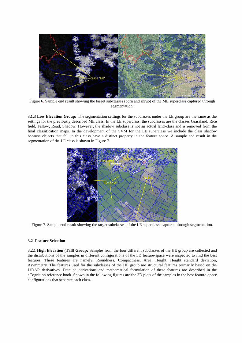
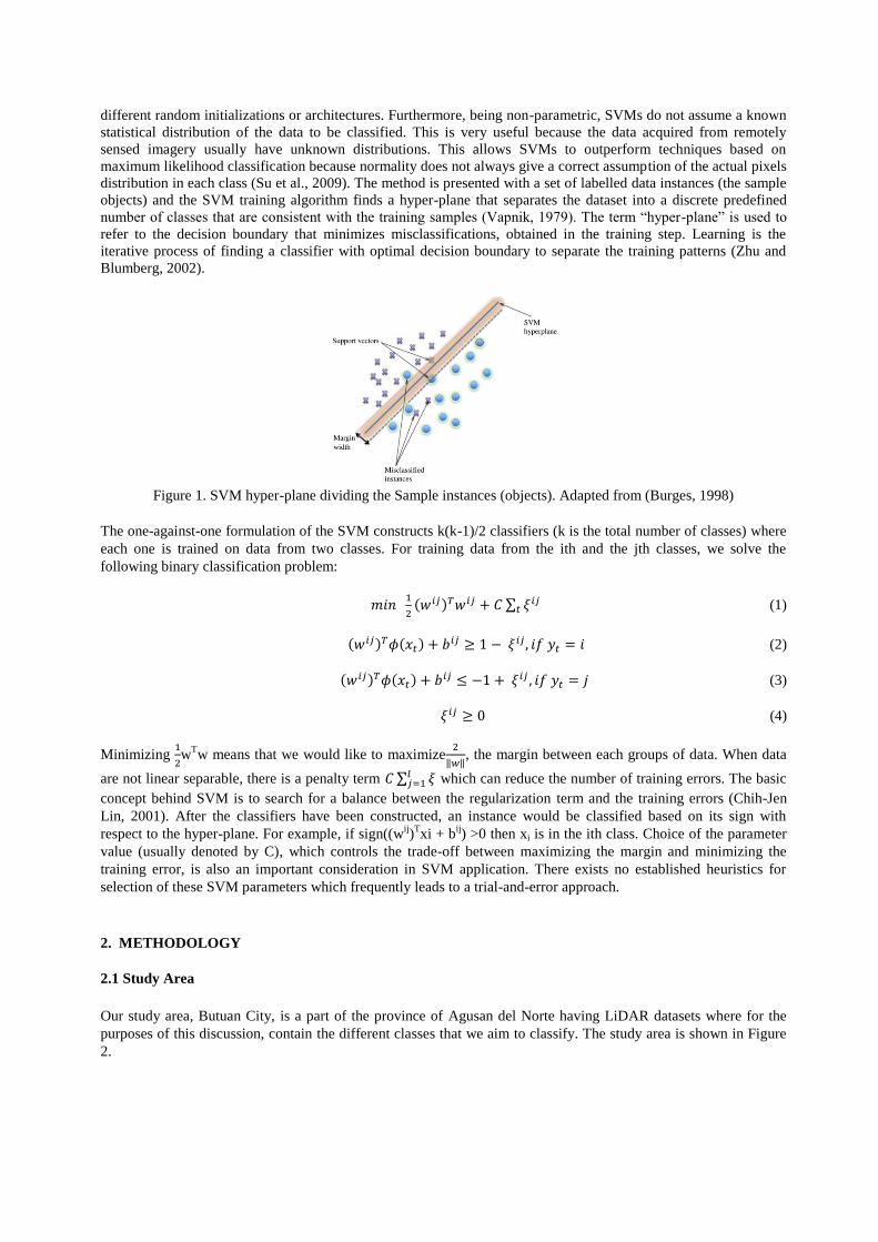
Figure 6. Sample end result showing the target subclasses (corn and shrub) of the ME superclass captured through

segmentation.

3.1.3 Low Elevation Group: The segmentation settings for the subclasses under the LE group are the same as the

settings for the previously described ME class. In the LE superclass, the subclasses are the classes Grassland, Rice

field, Fallow, Road, Shadow. However, the shadow subclass is not an actual land-class and is removed from the

final classification maps. In the development of the SVM for the LE superclass we include the class shadow

because objects that fall in this class have a distinct property in the feature space. A sample end result in the

segmentation of the LE class is shown in Figure 7.

Figure 7. Sample end result showing the target subclasses of the LE superclass captured through segmentation.

3.2 Feature Selection

3.2.1 High Elevation (Tall) Group: Samples from the four different subclasses of the HE group are collected and

the distributions of the samples in different configurations of the 3D feature-space were inspected to find the best

features. These features are namely; Roundness, Compactness, Area, Height, Height standard deviation,

Asymmetry. The features used for the subclasses of the HE group are structural features primarily based on the

LiDAR derivatives. Detailed derivations and mathematical formulation of these features are described in the

eCognition reference book. Shown in the following figures are the 3D plots of the samples in the best feature-space

configurations that separate each class.

Figure 8.Feature-space plots for the High Elevation (Tall) Group.

3.2.2 Medium Elevation Group: Much of the features used for SVM classification for the ME as well as the LE

super-class is based from color science and color image processing concepts. LiDAR intensity was used as well.

Findings of this study identified nine (9) features including LiDAR intensity for classifying the ME and LE

subclasses. Eight of the nine features come from color science concepts. To understand color measurement and

color management, it is necessary to consider human color vision. There are three things that affect the way a color

is perceived by humans. There are characteristics of the illumination and the object. Also, there is the interpretation

of this information in the eye/brain system of the observer. CIE metrics incorporate these three quantities,

correlating them well with human perception. The additional features used for the ME and LE are: Red Ratio (CIE

xy Chromaticity), Green Ratio (CIE xy Chromaticity), Blue Ratio (CIE xy Chromaticity), First Coordinate (1-

Dimensional Scalar Constancy), Second Coordinate (1-Dimensional Scalar Constancy), RGB Intensity (HSI), a*

(CIE Lab), b* (CIE Lab). Shown in Figure 9 are some of the 3D plots of the samples in the best feature-space

configurations that separate the classes corn and shrub.

Figure 9. Feature-space plots for the Medium Group (Corn and Shrub)

3.2.3 Low Elevation Group: The features used for the LE superclass are the same features used in developing the

model for the ME superclass. Shown in Figure 10 are the 3D plots of the samples in the best feature-space

configurations that separate the different subclasses in the LE superclass. In the plots, the class “uncultivated”

corresponds to the class fallow.

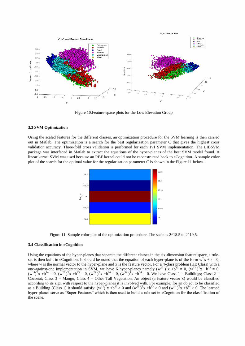
Figure 10.Feature-space plots for the Low Elevation Group

3.3 SVM Optimization

Using the scaled features for the different classes, an optimization procedure for the SVM learning is then carried

out in Matlab. The optimization is a search for the best regularization parameter C that gives the highest cross

validation accuracy. Three-fold cross validation is performed for each 1v1 SVM implementation. The LIBSVM

package was interfaced in Matlab to extract the equations of the hyper-planes of the best SVM model found. A

linear kernel SVM was used because an RBF kernel could not be reconstructed back to eCognition. A sample color

plot of the search for the optimal value for the regularization parameter C is shown in the Figure 11 below.

Figure 11. Sample color plot of the optimization procedure. The scale is 2^18.5 to 2^19.5.

3.4 Classification in eCognition

Using the equations of the hyper-planes that separate the different classes in the six-dimension feature space, a rule-

set is then built in eCognition. It should be noted that the equation of each hyper-plane is of the form wTx +b = 0,

where w is the normal vector to the hyper-plane and x is the feature vector. For a 4-class problem (HE Class) with a

one-against-one implementation in SVM, we have 6 hyper-planes namely (w12

)Tx +b

12 = 0, (w

13 )

Tx +b

13 = 0,

(w14

)Tx +b

14 = 0, (w

23 )

Tx +b

23 = 0, (w

24 )

Tx +b

24 = 0, (w

34 )

Tx +b

34 = 0. We have Class 1 = Buildings; Class 2 =

Coconut; Class 3 = Mango; Class 4 = Other Tall Vegetation. An object (a feature vector x) would be classified

according to its sign with respect to the hyper-planes it is involved with. For example, for an object to be classified

as a Building (Class 1) it should satisfy: (w12

)Tx +b

12 > 0 and (w

13 )

Tx +b

13 > 0 and (w

14 )

Tx +b

14 > 0. The learned

hyper-planes serve as “Super-Features” which is then used to build a rule set in eCognition for the classification of

the scene.

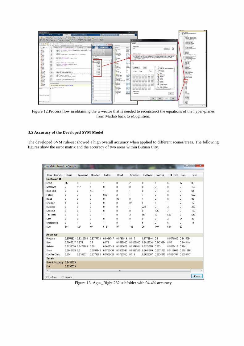
Figure 12.Process flow in obtaining the w-vector that is needed to reconstruct the equations of the hyper-planes

from Matlab back to eCognition.

3.5 Accuracy of the Developed SVM Model

The developed SVM rule-set showed a high overall accuracy when applied to different scenes/areas. The following

figures show the error matrix and the accuracy of two areas within Butuan City.

Figure 13. Agus_Right 282 subfolder with 94.4% accuracy

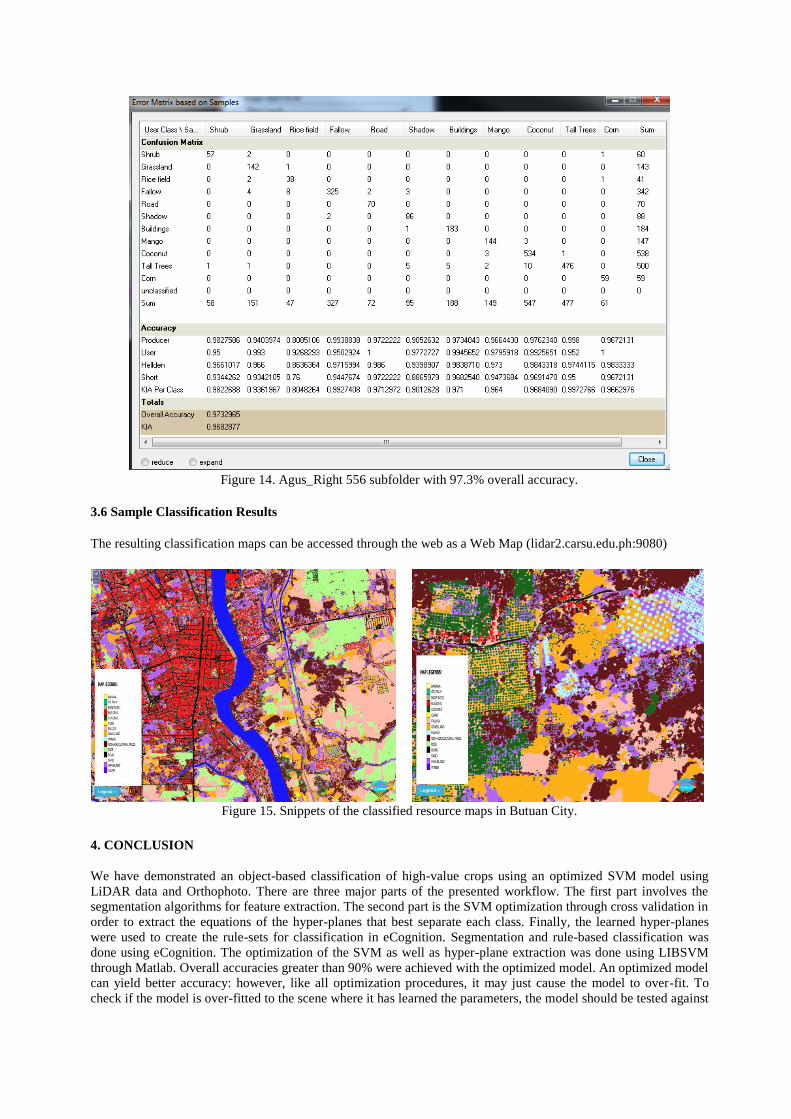
Figure 14. Agus_Right 556 subfolder with 97.3% overall accuracy.

3.6 Sample Classification Results

The resulting classification maps can be accessed through the web as a Web Map (lidar2.carsu.edu.ph:9080)

Figure 15. Snippets of the classified resource maps in Butuan City.

4. CONCLUSION

We have demonstrated an object-based classification of high-value crops using an optimized SVM model using

LiDAR data and Orthophoto. There are three major parts of the presented workflow. The first part involves the

segmentation algorithms for feature extraction. The second part is the SVM optimization through cross validation in

order to extract the equations of the hyper-planes that best separate each class. Finally, the learned hyper-planes

were used to create the rule-sets for classification in eCognition. Segmentation and rule-based classification was

done using eCognition. The optimization of the SVM as well as hyper-plane extraction was done using LIBSVM

through Matlab. Overall accuracies greater than 90% were achieved with the optimized model. An optimized model

can yield better accuracy: however, like all optimization procedures, it may just cause the model to over-fit. To

check if the model is over-fitted to the scene where it has learned the parameters, the model should be tested against

different scenes. We have shown that even when the optimized SVM model was tested against different scenes

within Butuan City, the obtained overall accuracies were greater than 94% as shown in section 3.5.

5. ACKNOWLEDGEMENT

The authors are grateful for the support of the Department of Science and Technology through the DOST-GIA and

the Philippine Council for Industry, Energy, and Emerging Technology Research and Development (DOST-

PCIEERD). LiDAR data was obtained from the UP DREAM-LiDAR Program.

6. REFERENCES

Blaschke, T.; Johansen, K.; Tiede, D.; Object-Based Image Analysis for Vegetation Mapping and Monitoring.

Advances in Environmental Remote Sensing: Sensors, 2011. - pp. 241-271.

Burges C., 1998. A Tutorial on Support Vector Machines for Pattern Recognition, Data Mining and Knowledge

Discovery, Kluwer Academic Publishers.

Chih-Chung Chang and Chih-Jen Lin, LIBSVM: A Library for Support Vector Machines, National Taiwan

University, Taipei, Taiwan, 2001.

Mountrakis et. al, 2009 : Support Vector Machines in Remote Sensing: A Review. ISPRS Journal of

Photogrammetry and Remote Sensing pp. 247-259.

Su, L., Huang, Y., 2009. Support vector machine (SVM) classification: comparison of linkage techniques using a

clustering–based method for training data selection. GIScience & Remote Sensing 46 (4), 411–423.

Trimble eCognition Reference Book 2014, Munich, Germany:[eBook].

Vapnik, V., 1979. Estimation of Dependencies Based on Empirical Data. Nauka, Moscow, pp.5165-5184.

Zhu, G., Blumberg, D.G., 2002. Classification using ASTER data and SVM algorithms; The case study of Beer

Sheva, Israel. Remote Sensing of Environment 80 (2), pp. 233–240.

Japitana, M and Candare, R.J., 2015. Optimization of the SVM Regularization Parameter C in Matlab for

Developing Rule-sets in eCognition, ISRS 2015 Proceedings, Tainan, Taiwan, pp. 530-533.