Optimization of the feeder assignment for PCB assembly...
56
Chalmers University of Technology University of Gothenburg Department of Computer Science and Engineering Göteborg, Sweden, April 2010 Optimization of the feeder assignment for PCB assembly machines Master of Science Thesis in the Computer science and engineering KRISTOFFER WIKLUND
Transcript of Optimization of the feeder assignment for PCB assembly...

Chalmers University of Technology
University of Gothenburg
Department of Computer Science and Engineering
Göteborg, Sweden, April 2010
Optimization of the feeder assignment for PCB
assembly machines
Master of Science Thesis in the Computer science and engineering
KRISTOFFER WIKLUND
The Author grants to Chalmers University of Technology and University of Gothenburg
the non-exclusive right to publish the Work electronically and in a non-commercial
purpose make it accessible on the Internet.
The Author warrants that he/she is the author to the Work, and warrants that the Work
does not contain text, pictures or other material that violates copyright law.
The Author shall, when transferring the rights of the Work to a third party (for example a
publisher or a company), acknowledge the third party about this agreement. If the Author
has signed a copyright agreement with a third party regarding the Work, the Author
warrants hereby that he/she has obtained any necessary permission from this third party to
let Chalmers University of Technology and University of Gothenburg store the Work
electronically and make it accessible on the Internet.
Optimization of the feeder assignment for PCB assembly machines
KRISTOFFER E. WIKLUND
© KRISTOFFER E. WIKLUND, October 2009.
Examiner: DEVDATT DUBHASHI
Chalmers University of Technology
University of Gothenburg
Department of Computer Science and Engineering
SE-412 96 Göteborg
Sweden
Telephone + 46 (0)31-772 1000
Cover:
Machine layout for mounting components onto a PCB, see page 29
Department of Computer Science and Engineering
Göteborg, Sweden October 2009

REPORT NO. xxxx/xxxx
Optimization of the feeder assignment for PCB assembly machines
KRISTOFFER WIKLUND
The Department of Computer Science and Engineering
CHALMERS UNIVERSITY OF TECHNOLOGY
Göteborg, Sweden 2009

CHALMERS, Optimization of the feeder assignment for PCB assembly machines,
Master Thesis 2009: I
Abstract
This report is part of a master thesis done at Chalmers University of Technology in Göteborg
and in cooperation with Valor Computerized Systems. The purpose with the report was to
compare different algorithms performance in solving a subproblem in PCB assembly. PCB
assembly is about to balance the PCB production between different production lines in a
factory. For each line one need to balance electrical parts’ assembly between the machines in
the production line. Finally a minimized sequence of the assembly of components is
constructed. The subproblem for this thesis has been the feeder assignment problem, where
the problem is come up with setup for how and in which feeder slots the components for the
production should be placed, for minimizing the production time. The subproblem has been
showed to be NP-hard been proven that the Traveling Salesman problem can be transformed
to the subproblem.
We have chosen to compare two versions of Local Search algorithms and two versions of
genetic algorithms and a simple heuristic algorithm. To obtain a reliable comparison, the
solutions are imported into Valor’s software to solve and model a complete assembly
machine. Valor’s software has enabled us to obtain the simulated production times. To be able
to use the chosen algorithm a new and simplified cost function has been developed.
Our approach has showed that is possible to lower the production time compared to Valor’s
current software. To draw a concussion of which algorithm to use is not possible. All five
algorithms have given around one percent improvements. One explanation for that is that the
simplified cost function has simplified the problem to much so that it is not possible to
separate a good feeder assignment hungry against a less good solution.
Keywords: PCB, Assembly, Optimization problem, Feeder assignment, Local Search,
Genetic Algorithm, NP-Hard, TSP

CHALMERS, Optimization of the feeder assignment for PCB assembly machines,
Master Thesis 2009: II
Sammanfattning
Denna rapport är en del av ett examensarbete utfört på Chalmers tekniska högskola i
samarbete med Valor Computerized Systems. Syftet med rapporten var att jämföra olika
algoritmers förmåga att lösa ett utav delproblemen inom kretskortstillverkning.
Kretskortstillverkning handlar om att fördela kretskorts tillverkning mellan olika
produktionslinjer i en fabrik. För varje linje handlar det om att fördela komponenternas
montering mellan maskinerna i en produktionslinje. Slutgiltigt så ska en minimerad sekvens
av montering av komponenter konstrueras. Rapporterns delproblem, matar
fördelningsproblemet, har varit att lösa hur och i vilka matare som komponenter ska placeras
i, så att produktionstiden är minimerad. Delproblemet är bevisat att vara NP-svårt genom att
bevisa att Handelsresandeproblemet kan transformeras till delproblemet.
Vi har valt att jämföra två versioner Local Search algoritmer och två versioner av generiska
algoritmer och en enkel heuristik algoritm. För att få en trovärdig jämförelse har lösningarna
importeras till Valor’s programvara för att lösa och modellera upp en fullständig
monteringsmaskin. Genom Valor’s programvara har vi kunnat erhålla simulerade
produktionstider. För att kunna använda valda algoritmer har också en egen förenklad
kostfunktion utvecklats.
Vår tillgångavägsätt sätt har visat på att det går att sänka produktionstiden jämföra med
Valors nuvarande programvara. Vilken algoritm som ska användas går inte att dra slutsatser
ifrån då de alla fem ligger på runt en procents förbättring. En förklaring till detta har varit den
förenklade kostfunktionen vilket trors ha förenklat problemet för mycket och gjort att bra
lösningar inte kan skiljas från mindre bra lösningar.
Nyckelord: PCB, Kretskort, Tillverkning, Optimerings problem, Local Search, Generiska
algoritmer, NP-Hard, TSP

CHALMERS, Optimization of the feeder assignment for PCB assembly machines,
Master Thesis 2009: III
Content Abstract ....................................................................................................................................... I
Sammanfattning ........................................................................................................................ II
Content ..................................................................................................................................... III
Preface ....................................................................................................................................... V
Notations and definitions ......................................................................................................... VI
List of Figures, Tables and Equations ..................................................................................... VII
1 Introduction ............................................................................................................................. 1
1.1 Background ....................................................................................................................... 4
1.2 Purpose ........................................................................................................................... 12
1.3 Delimitations .................................................................................................................. 14
1.4 Local Search ................................................................................................................... 14
1.5 Genetic Algorithms ......................................................................................................... 15
1.6 Heuristic .......................................................................................................................... 19
2 The Traveling salesman problem transformation .................................................................. 20
2.1 General TSP .................................................................................................................... 20
2.2 Placement TSP ................................................................................................................ 20
2.3 Feeder bank assignment .................................................................................................. 20
3 Methods ................................................................................................................................. 22
3.1 Internal structure ............................................................................................................. 22
3.2 Time factors .................................................................................................................... 24
3.3 Cost function for evaluating feeder assignments ............................................................ 25
3.4 Revolver setup ................................................................................................................ 27
3.5 Algorithms ...................................................................................................................... 27
3.6 Lower bound ................................................................................................................... 28
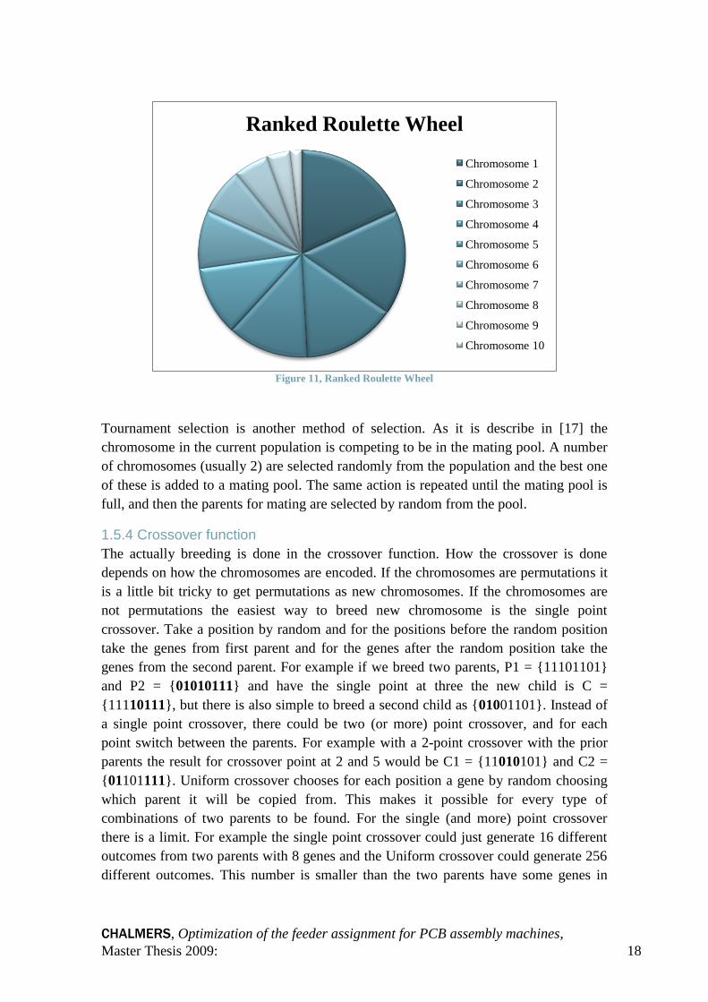
3.7 Test data .......................................................................................................................... 29

CHALMERS, Optimization of the feeder assignment for PCB assembly machines,
Master Thesis 2009: IV
4 Results ................................................................................................................................... 31
4.1 Performance of the algorithms subject to the cost function ........................................... 32
4.2 Relation between cost function and production time ..................................................... 33
4.3 Performance of the algorithms to solve the whole problem ........................................... 37
5 Discussion ............................................................................................................................. 38
6 Conclusions ........................................................................................................................... 40
7 Future Work .......................................................................................................................... 41
8 References ............................................................................................................................. 42
Appendix 1: Algorithms ........................................................................................................... 44

CHALMERS, Optimization of the feeder assignment for PCB assembly machines,
Master Thesis 2009: V
Preface
This Master Thesis was carried out from April 2009 until October 2009 at the Department of
Computer Science and Engineering, Chalmers University of Technology in Göteborg,
Sweden. Working place for the thesis has been at the R&D department office in Turku,
Finland for Valor Computerized Systems. The work has been formulated and supervised by
Ph.D. Mika Johnsson at Valor Computerized Systems. Examiner of the thesis is Prof. Devdatt
Dubhashi at Chalmers University of Technology.
A special gratitude is dedicated to Prof. Olli Nevalainen at Turku University who has been
helping and supervising me, thanks for reading and correcting my report.
I would like to thank Mika Johnsson and Valor Computerized System for giving me the
opportunity to work with this thesis’s subject. It has been an interested problem, I am thankful
for getting the help concerning my research topic, books and hardware needed when
conducting this study.
I also like to thank my loving wife, Marianne, which have supported me during the work.
Turku October 2009
Kristoffer Wiklund

CHALMERS, Optimization of the feeder assignment for PCB assembly machines,
Master Thesis 2009: VI
Abbreviations and definitions
Abbreviations
AI Artificial Intelligence
CAD Computer-aided design
GA Genetic algorithm
LS Local Search
PCB Printed circuit board
PMX Partially mapped crossover
RAM Random-access memory
SMT Surface-mount technology
Definitions
Component An electronic element that has one or more connections.
Part Type definition of components, all components of the same part
have the same form and specification
Placement Description that a given component needs to be placed on
a given position on the PCB
PCB job Description of a set of parts that will be mounted onto the PCB
Feeder Component supply mechanism in SMT machines
Placement head Mechanical arm of a SMT machine that places the components
Spindle Mechanical part attached to the placement head for picking and
placing a single component
Nozzle Gripping tool for allowing spindles to pick a kinds of components

CHALMERS, Optimization of the feeder assignment for PCB assembly machines,
Master Thesis 2009: VII
List of Figures, Tables and Equations
List of Figures
Figure 1, Example of production line ......................................................................................... 1
Figure 2, Machine layout ........................................................................................................... 2
Figure 3, Dual Delivery placement machine .............................................................................. 6
Figure 4, Turret style placement machine [5] ............................................................................ 7
Figure 5, Sequential Pick-And-Place Machine [5] ..................................................................... 7
Figure 6, Multi-Head Placement Machine [5]............................................................................ 8
Figure 7, Multi-Station Placement Machine [5] ......................................................................... 9
Figure 8, Hierarchy of the problems found in PCB assembly ................................................... 9
Figure 9, Feeder assignment problem ...................................................................................... 13
Figure 10, Roulette wheel ........................................................................................................ 17
Figure 11, Ranked Roulette Wheel .......................................................................................... 18
Figure 12, Flow of the experimental tests ................................................................................ 22
Figure 14, MachineConfiguration class. .................................................................................. 23
Figure 13, PCB class ................................................................................................................ 23
Figure 15, Algorithms classes .................................................................................................. 24
Figure 16, Graphical presentation of PCB-9 in the developed software .................................. 29
Figure 17, Relation between procedure S and production time for all PCBs .......................... 34
Figure 18, Relation between procedure S and production time for PCB-1 .............................. 35
Figure 19, Relation between procedure S and production time for PCB-2 .............................. 35
Figure 20, Relation between procedure S and production time for PCB-5 .............................. 36
Figure 21, Relation between procedure S and production time for PCB-8 .............................. 36
List of Tables
Table 1, PCBs in number ......................................................................................................... 31
Table 2, TEST results with procedure S .................................................................................. 32
Table 3, PCB results with procedure S .................................................................................... 32
Table 4, TSP problem results ................................................................................................... 33
Table 5, Average difference in production time for exact same feeder assignment ................ 33
Table 6, Performance of the algorithms solving the final problem .......................................... 37
List of Equations
Equation 1, Ranked Roulette Wheel formula ........................................................................... 17
Equation 2, Total time .............................................................................................................. 24
Equation 3, Time for a revolver ............................................................................................... 24
Equation 4, Pick-up phase ........................................................................................................ 25
Equation 5, Placement phase .................................................................................................... 25
Equation 6, Lower bound ......................................................................................................... 28
CHALMERS, Optimization of the feeder assignment for PCB assembly machines,
Master Thesis 2009: 1
1 Introduction
Articles about Printed Circuit Board, PCB, [1], [2], almost always discuss the increased
demand, new development and increased production volumes in the PCB assembly
industry. One common explanation for the rapid development in the field is that citizens
own more and more electrical devices and almost each of those devices includes a PCB
in it. Design and construction of PCB is very universal and enables almost every
possible electrical circuit.
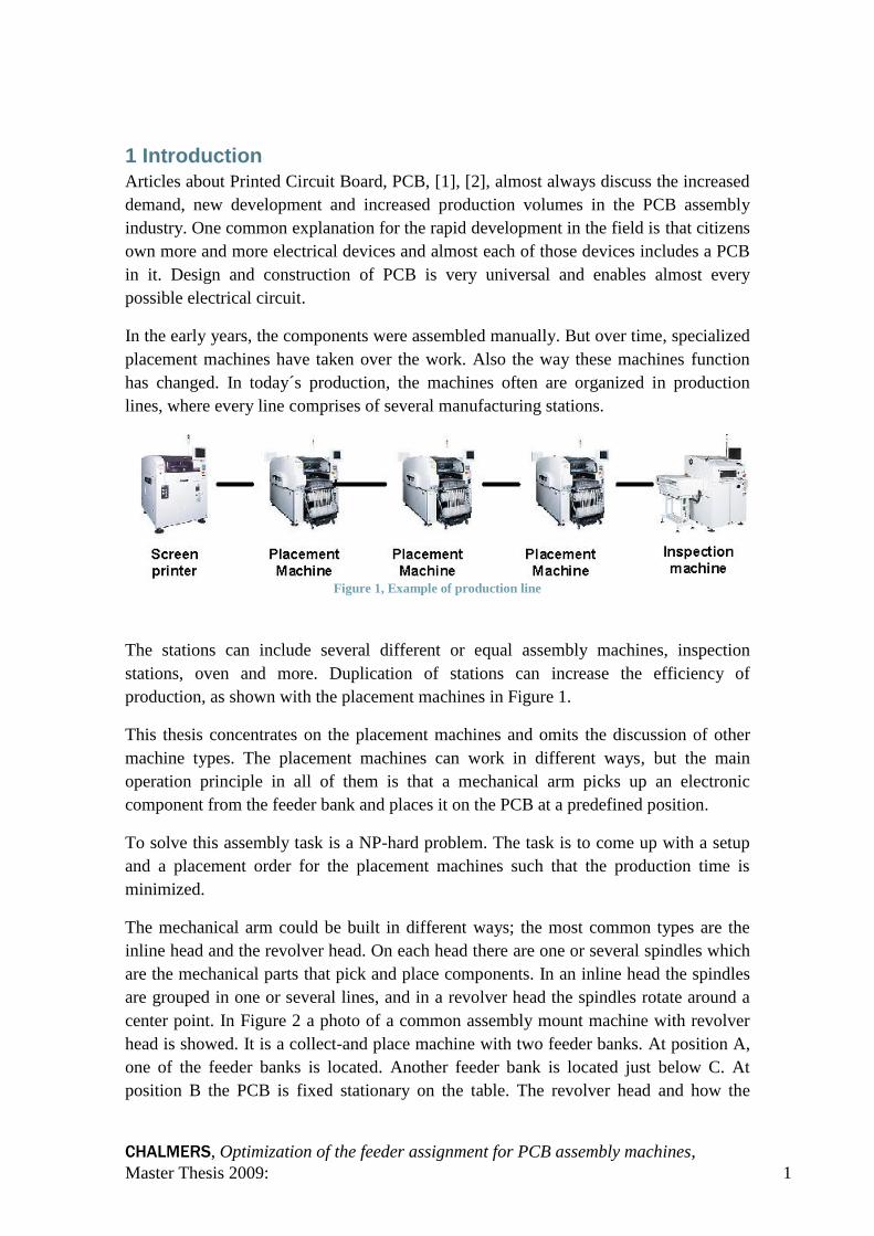
In the early years, the components were assembled manually. But over time, specialized
placement machines have taken over the work. Also the way these machines function
has changed. In today´s production, the machines often are organized in production
lines, where every line comprises of several manufacturing stations.
Figure 1, Example of production line
The stations can include several different or equal assembly machines, inspection
stations, oven and more. Duplication of stations can increase the efficiency of
production, as shown with the placement machines in Figure 1.
This thesis concentrates on the placement machines and omits the discussion of other
machine types. The placement machines can work in different ways, but the main
operation principle in all of them is that a mechanical arm picks up an electronic
component from the feeder bank and places it on the PCB at a predefined position.
To solve this assembly task is a NP-hard problem. The task is to come up with a setup
and a placement order for the placement machines such that the production time is
minimized.
The mechanical arm could be built in different ways; the most common types are the
inline head and the revolver head. On each head there are one or several spindles which
are the mechanical parts that pick and place components. In an inline head the spindles
are grouped in one or several lines, and in a revolver head the spindles rotate around a
center point. In Figure 2 a photo of a common assembly mount machine with revolver
head is showed. It is a collect-and place machine with two feeder banks. At position A,
one of the feeder banks is located. Another feeder bank is located just below C. At
position B the PCB is fixed stationary on the table. The revolver head and how the

CHALMERS, Optimization of the feeder assignment for PCB assembly machines,
Master Thesis 2009: 2
spindles are located around it can be seen at C. In the image, the revolver is picking
components at the feeder bank and will later go to the PCB at B and place the
components and after that go to the feeder bank at A again to pick up some new
components.
Placement machines can be classified into 5 categories [3]. The five classes are: Dual
Delivery Placement Machine, Multi-Station Placement Machine, Turret Style
Placement Machine, Multi-Head Placement Machine, and Sequential Pick-and-Place
Machine. Each of these solves the assembly task in a different way. This thesis will
discuss how to solve assembly task for Multi-Head Placement Machines.
PCB assembly control problems have been divided into three subproblems in [2]. The
first problem is to group the PCBs by the similarity of the components and then choose
the machine group/production line. The next problem is to optimally divide the
placements of the components between the machines so that there is no big bottleneck
machine in the group. The last problem is to decide the feeder, nozzle and placement
sequence for each machine.
Figure 2, Machine layout

CHALMERS, Optimization of the feeder assignment for PCB assembly machines,
Master Thesis 2009: 3
All these problems depend on each other when one tries to solve them in a total optimal
way. In order to know which components a machine should place it is necessary to
group the PCBs and machines. For optimal grouping of the PCBs one has to know how
to divide the placements between the machines in the group. It is impossible to solve
one of these subproblems without considering its relation to the other problems.
This thesis deals with the last subproblem, the feeder arrangement, nozzle arrangement
and placement sequence optimization. The problem will be divided into two
subproblems. The first problem is to fix the feeder and nozzle bank setting. The second
problem is to optimize the placement order with respect to the components and feeder
bank. The task in this thesis is to develop, test and compare different algorithms for
fixing the feeder and nozzle bank. In order to see how well the solutions really are, one
has to solve also the second subproblem. For solving the second subproblem we will use
Valor’s planning software to generate a placement sequence and to calculate the total
assembly time for that PCB job.
This thesis has the following structure. Chapter 1 explains the background of the PCB
assembly research and how PCB assembly works out in the real-life industry. The
purpose and delimitations of the thesis is explained and also a description of the
algorithms and techniques is given. Chapter 2 will explain how to transform the TSP
problem into a PCB assembly problem and show that the PCB assembly problem is NP-
hard. Chapter 3 is in detail describing how the problem has been modeled and how we
have adapted the algorithms. The heuristics and the formulas we used are presented in
this chapter. Chapter 4 describes the results of the practical tests; how well our
algorithms run and what works and what does not. Chapter 5 discusses the relation
between the methods and the results and how the results relate to the problem. It
describes the results and how it refers to the problem. Chapter 6 shows what conclusion
one could draw from the results. Chapter 7 discusses how one could do more research
on this subject, how to develop the algorithms, how to implement the software tools in
the industry and how to improve the algorithms.

CHALMERS, Optimization of the feeder assignment for PCB assembly machines,
Master Thesis 2009: 4
1.1 Background
The desire to connect electronic components in an easy way has existed from the early
days of electronics. The technique with PCB was invented by Paul Eisler around the
Second World War. After the Second World War the technique was released for
commercial use. In this technique, copper traces are printed on a non-conductive board,
where the traces connect the different components mounted on the board.
A PCB is as the name says a circuit board with a printed electrical circuit. The board is
often green in color and has lots of different components mounted on it and it is placed
in a machine behind a plastic cover. One can find PCBs in a broad range of customer
products including for example computers, cars, phones, dish washer, clocks and more.
There are many different types of circuit boards. Components can be attached by
through-hole construction or by surface-mount construction/ surface-mount technology
(SMT). The material for the board and for the electrical traces can differ. This report
focuses not on the construction of PCBs; instead, it focuses on the assembly of
components on the PCB. The optimization in this thesis will be made for an SMT-
machine, but the results can be applied to through-hole technology as well.
Manual assembly of components on the PCB was the first approach of the technology
and it is still used for special cases. As machines have been developed and become more
advanced, more and more components can be mounted by the machine with greater
accuracy, speed and with fewer faults. As the machines get more and more advanced an
optimization problem is risen; how to sequence the component placements in an optimal
manner. The same problem exists also for manual assembly, but it is not as critical,
instead developing of routines and techniques for lowering the risk of human error have
been investigated. [4]
One important thing to keep in mind is the difference between part, component and
placement. A component is an electronic element that has one or more connection; this
is like an atom for electronics. Part is the type definition for components, all
components of the same part has the same form and specification. Placement is a word
for describing that a component has a fixed placement position on the board. Therefore
a PCB consist of a number of parts that each has one or several placements. A PCB
consists of the same number of components that it has placements in total.
Some components that are going to be placed on the board need to be visually verified
so that the right component is placed and that the component has the right angle.
Therefore machines often have a camera to take a picture of the components. The
camera might only take black and white pictures, and many times it just examines the
shape of the component. Taking pictures of components can be done in different ways;
sometime there is a fixed camera station where the mechanical arm verifies the
components before placing them. Other machines can have a moving camera station so
CHALMERS, Optimization of the feeder assignment for PCB assembly machines,
Master Thesis 2009: 5
that the verification of components can be done while the arm is moving. There are even
more ways of visual verification of the components that the vendors use.
The mechanical arm, the placement head, can be constructed in several different ways
but in most cases they are either of inline or revolver type. A placements head has one
or several spindles. Spindles are the mechanics for picking up a single component, but
in order for the spindle to be able to pick up the component it needs a griping tool. For
that purpose the industry has developed different kinds of nozzles for picking and
placing the components. It works by using a vacuum of air to suck up a component from
the feeder slot and air pressure to place the component on the PCBs. Several kinds of
nozzles can pick up the same type of components and nozzles can pick up several
different component types. The nozzles have different specifications and they set
limitations to the placement head in regard to movement and rotation speed. Special
components that are hard to hold also affect the selection of the placement head and
give it more limitations. The spindles often have the ability to rotate, which makes it
possible to have the right angle of the component when placing it on the PCB.
The difference between inline head and a revolver head is that for an inline head the
spindles are grouped in one or more lines. This feature makes it possible to do gang-
picks. In gang-picks several spindles pick up components simultaneous. If two spindles
are picking components at the same time the time is lowered by 50% for that task and if
6 spindles pick their components at the same moment of times the task consumes 16%
of the time it would take to pick them up sequentially. In revolver heads the spindles are
located in a rotating circle, so that the spindles are rotating around a center point. Some
revolver head types have a camera located at the top of the head. This makes it possible
to do the camera verification of the component placed on the top spindle while the
bottom spindle is picking up a component.
In order to place the components in exactly the right positions there is a set of fiducial
marks on the PCBs. After the PCB is loaded to the machine, the head locates the
fiducial marks by a camera. This takes some production time at the beginning of
processing each PCB but the machines are then able to place components extremely
accurately.
SMT machines are equipped with one or several feeder banks. They supply the
component to the machine. A feeder bank is divided into several feeder slots which are
the mechanical places for holding components. Each slot can be populated with a
feeding unit. A common industry feeder unit is the tape feeder. Here the components are
attached onto a long tape like a movie theater tape. The placement head picks a
component and after this the tape is rotated so that a new component can be picked.
There are tapes of different widths, and therefore some parts take up several feeder
slots. There are also some feeders that can take two or more parts (i.e. component tape
reels) in the same feeder slot.
CHALMERS, Optimization of the feeder assignment for PCB assembly machines,
Master Thesis 2009: 6
1.1.1 Machine Classification
As mentioned in the introduction, there are several different types of assembly
machines. SMT machines have been classified into five classes [3]: Dual Delivery
Placement Machine, Multi-Station Placement Machine, Turret Style Placement
Machine, Multi-Head Placement Machine, and Sequential Pick-and-Place Machine.
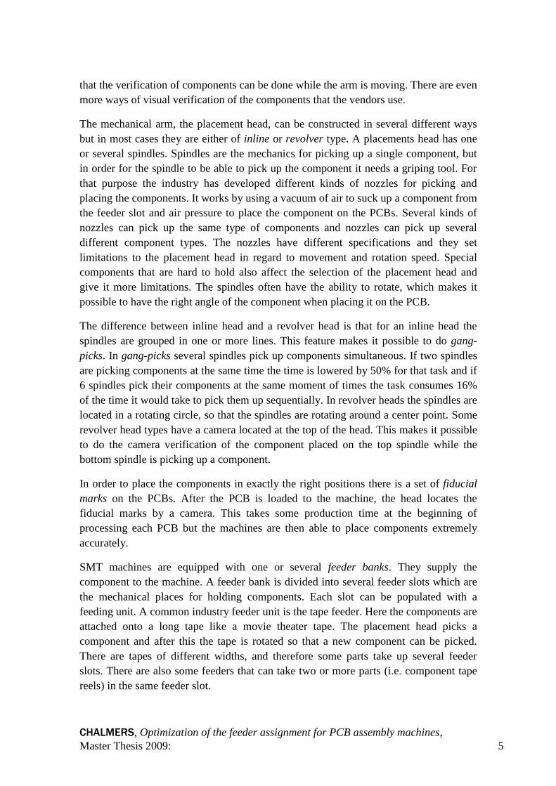
Dual Delivery Placement (Figure 3) has a movable PCB table that can move in x- and
y-direction. In the machine there are two placement arms, located on the opposite sides
of the table. They can move in y-direction between the placement position and the
pickup position over a movable feeder bank. When one arm is placing components the
PCB table is moved to its side, and the other arm is picking up components. After the
component has been placed, the PCB table moves to the other side there the other arm
places its component.
Figure 3, Dual Delivery placement machine
A Turret Style Placement Machine (Figure 4) has a big rotating turret with several
spindles on it. On one side of the turret there is a moving feeder bank and on the other
side is the PCB table, which moves in the x- and y-direction. The feeder bank is situated
on the side of the machine, the spindles pick up components and the moving feeder
bank is moved in the x-direction so that the correct part is under the spindle. The PCB
table is moved so that the placing position for the component in the spindle is under the
spindle and then the component is placed to its proper position.

CHALMERS, Optimization of the feeder assignment for PCB assembly machines,
Master Thesis 2009: 7
Figure 4, Turret style placement machine [5]
A Sequential Pick-and-Place Machine (Figure 5) consists of a moving arm. The arm can
move over a fixed PCB table, a fixed feeder bank and a fixed nozzle bank. The arm has
one spindle that picks up and places components. The placements are done in pick-and-
place blocks, where the placement head first moves to the feeder bank, picks up a
component, then goes to the PCB table and places the component on its correct position.
Figure 5, Sequential Pick-And-Place Machine [5]
CHALMERS, Optimization of the feeder assignment for PCB assembly machines,
Master Thesis 2009: 8
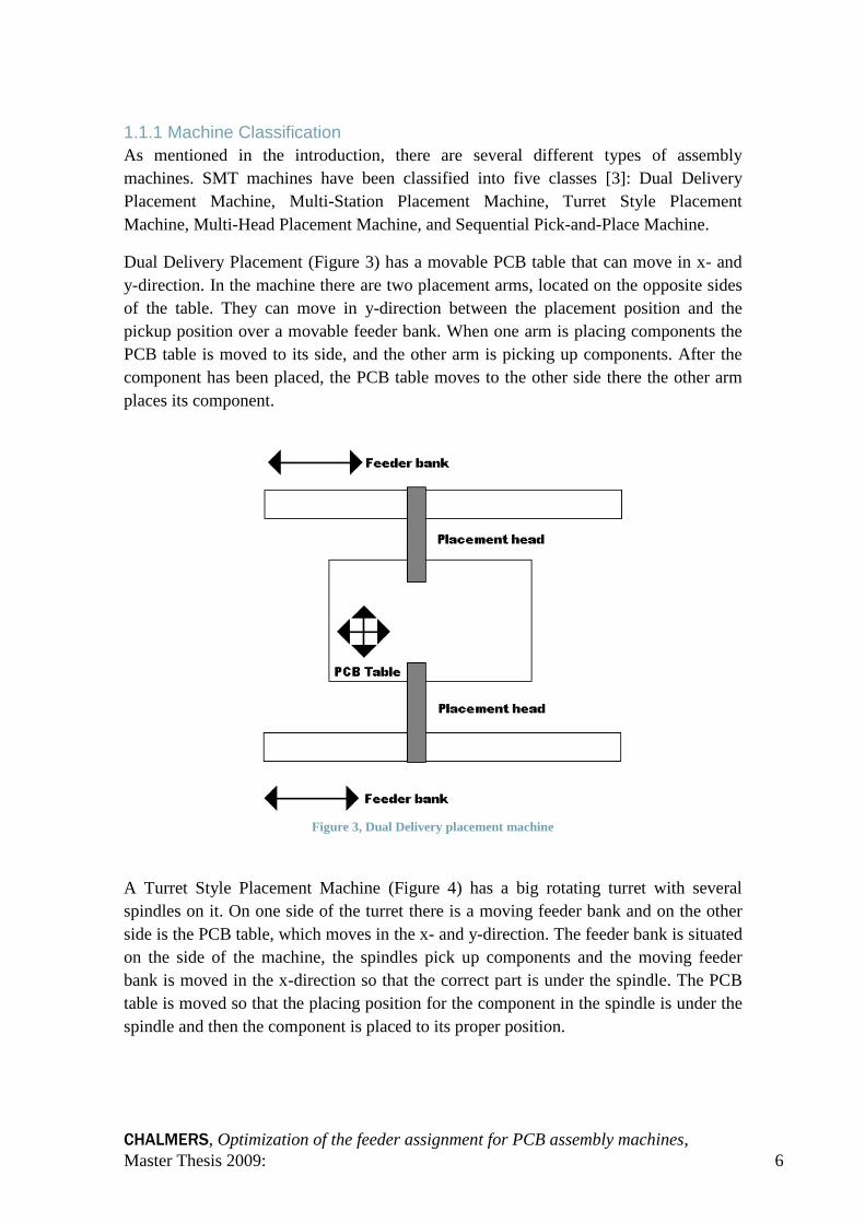
Multi-Head Placement Machine (Figure 6) is almost of the same technology as the
Sequential Pick-And-Place machines. But instead of just one spindle on the placement
head it has multiple spindles. These machines are sometimes called collect-and-place
machines because they collect a number of components from the feeder bank and then
place them on the PCB. Spindles can be arranged into one or several rows or they can
be on a rotating revolver. For the revolver head the head needs to rotate the head before
picking and placing. Inline heads can perform gang-picks.
Figure 6, Multi-Head Placement Machine [5]
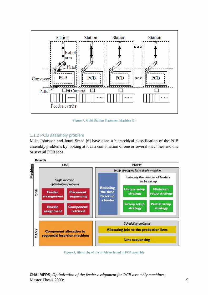
A Multi-Station Placement Machine (Figure 7) consists of several modules or stations.
Each module has an arm that can move in x- and y-directions. The arm is picking and
placing a limited set of components on the fixed PCB board. When a station has placed
all of its components for a certain PCB, the PCB is moved to the next station. This
machine is like several Sequential Pick-and-Place Machines in one.
CHALMERS, Optimization of the feeder assignment for PCB assembly machines,
Master Thesis 2009: 9
Figure 7, Multi-Station Placement Machine [5]
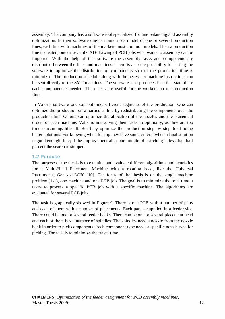
1.1.2 PCB assembly problem
Mika Johnsson and Jouni Smed [6] have done a hierarchical classification of the PCB
assembly problems by looking at it as a combination of one or several machines and one
or several PCB jobs.
Figure 8, Hierarchy of the problems found in PCB assembly

CHALMERS, Optimization of the feeder assignment for PCB assembly machines,
Master Thesis 2009: 10
Figure 8 shows how they have classified the problem, and how it can be broken down
into subproblems. This differs to the classification made before [3] and is another way
to describe the PCB assembly task.
One PCB job and one machine (1-1). In this problem we have one machine and want to
produce one type of PCB as effectively as possible. The goal is to minimize the
assembly time. For this setup we have four subproblems. The feeder assignment
problem is to organize the parts to the feeder slots in an optimal way so that the travel
time is minimized and gang-picks or other techniques can be used. The placement
sequence problem is to solve the order to place the components such that the head
movement time is minimized. The nozzle assignment problem is to choose the nozzles
to be used. The component retrieval problem exists if the machine has duplications of
parts in several feeder slots, and it is optimized how the picks should be done.
Many PCB jobs and one machine (M-1). The goal in this problem is to minimize the
time for production, but compared to the Single-machine problem one now has to
consider the time to setup the machines. There are two possible way to minimize the
setup time, either one minimizes the time it takes to setup the machine or minimizes the
number of needed setups. The minimizing of setup time for one machine is about
hardware and organization on the factory floor. The second problem has been
researched and is about grouping and balancing [7]. As Johnsson and Smed [6] write
there are different strategies to solve that problem; unique setup strategy, minimum
setup strategy, group setup strategy, and partial setup strategy.
The One PCB job and many Machines problem (1-M) deals with load balancing. The
goal is to divide the parts between the different machines such that the production time
is as equal and low as possible, because the time to produce a PCB is determined by the
machine taking the longest time, the bottleneck machine. For each machine there is the
(1-1) problem to be solved with the set of parts that the machine should produce.
Many PCB jobs and many machines (M-M) is the most advanced and difficult version
of the problem but it is also the problem that is most common in the industry. Here one
has to decide the jobs to the different lines and to decide which PCB jobs each line
should produce.
The classification that Johnsson and Smed [6] have done is to classify the problem but
M Ayob, P Cowling and G Kendal [3] has done a machine classification. The five
machine classification can be described into the hierarchy by looking how they work for
a single PCB job. Dual Delivery Placement Machine, Sequential Pick-and-Place
Machine, Multi-Head Placement Machine and Turret Style Placement Machine are only
facing the (1-1) problem as a single machine. For the Multi-Station Placement Machine
there is always the need to solve the (1-M) problem, because every PCB is processed by
several stations and each stations is like its own machine.

CHALMERS, Optimization of the feeder assignment for PCB assembly machines,
Master Thesis 2009: 11
This thesis concentrates on the one machine and one PCB job (1-1) problem for a Multi-
Head Placement Machine. There are many parameters and settings for this problem as
mention before, but the goal is here to minimize the production time for a single PCB
job. Either one could improve the machine with better hardware, like more feeder slots,
faster moving/rotating placement heads or maybe more placements head in the machine.
This approach is pushed by the machine vendors and it is often the more expensive way.
The other way is that one tries to improve the usages of the available resources. There
are studies that show that by optimizing the placement sequence or the planning of
production one could get an improvement on 10% and up over 50% [8].
To do a realistic model of the problem can be very hard. This is because the machines
can differ in many ways between each model and vendor. The movements made by the
machine are also very complex; acceleration and deacceleration are non-linear. The arm
movement from point A to point B cannot be expressed by a simple formula, neither do
the machine vendors have any movement graph to hand out, as it is treated as a trade
secret or they simply don’t have it.
But some type of model of the machine is required to solve the problem, and to test the
solutions. An important thing to think at is that all machine operations consumes some
time. Many times several operations can be done simultaneously which makes that the
time for a group of operations is determined by the operation that takes the longest time.
As an example; if the placement head needs to moves 4 steps in x-direction and 5 steps
in y-direction this movement is done by two moving parts in the machine, one in x-
direction and the other in y-direction. The time for this is the maximum of the time to
move in the two directions.
One need to do some simplification of the problem but if the simplification is done
without research, the results of the model could be really bad, so that a solution of the
model seems to be very good but in reality it does not work in practice.
Here is a short list of common tasks in SMT machines that take some time:
Placement of a component on the PCB
Pick up of a component in feeder bank
Movement of the arm into correct position
Movement of the PCB table (for the machine that have it)
Rotation of the head
Preparation of the component in feeder slot
Changing of the nozzle
Loading and reading fiducial marks of the PCB
Rotation of components
Valor Computerized Systems [9] has developed software for PCB manufacturers. Their
software helps the manufactures the whole way from PCB design, planning and
CHALMERS, Optimization of the feeder assignment for PCB assembly machines,
Master Thesis 2009: 12
assembly. The company has a software tool specialized for line balancing and assembly
optimization. In their software one can build up a model of one or several production
lines, each line with machines of the markets most common models. Then a production
line is created, one or several CAD-drawing of PCB jobs what wants to assembly can be
imported. With the help of that software the assembly tasks and components are
distributed between the lines and machines. There is also the possibility for letting the
software to optimize the distribution of components so that the production time is
minimized. The production schedule along with the necessary machine instructions can
be sent directly to the SMT machines. The software also produces lists that state there
each component is needed. These lists are useful for the workers on the production
floor.
In Valor’s software one can optimize different segments of the production. One can
optimize the production on a particular line by redistributing the components over the
production line. Or one can optimize the allocation of the nozzles and the placement
order for each machine. Valor is not solving their tasks to optimally, as they are too
time consuming/difficult. But they optimize the production step by step for finding
better solutions. For knowing when to stop they have some criteria when a final solution
is good enough, like; if the improvement after one minute of searching is less than half
percent the search is stopped.
1.2 Purpose
The purpose of the thesis is to examine and evaluate different algorithms and heuristics
for a Multi-Head Placement Machine with a rotating head, like the Universal
Instruments, Genesis GC60 [10]. The focus of the thesis is on the single machine
problem (1-1), one machine and one PCB job. The goal is to minimize the total time it
takes to process a specific PCB job with a specific machine. The algorithms are
evaluated for several PCB jobs.
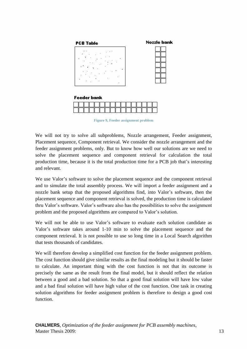
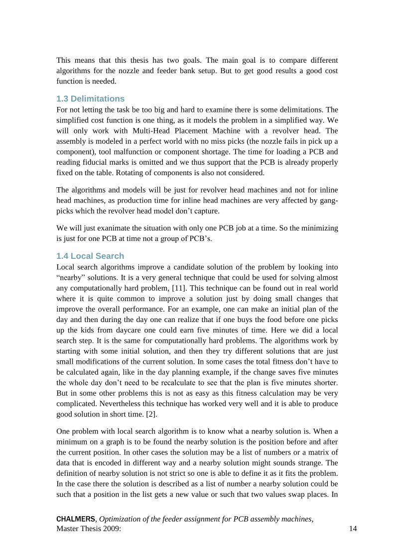
The task is graphically showed in Figure 9. There is one PCB with a number of parts
and each of them with a number of placements. Each part is supplied in a feeder slot.
There could be one or several feeder banks. There can be one or several placement head
and each of them has a number of spindles. The spindles need a nozzle from the nozzle
bank in order to pick components. Each component type needs a specific nozzle type for
picking. The task is to minimize the travel time.
CHALMERS, Optimization of the feeder assignment for PCB assembly machines,
Master Thesis 2009: 13
We will not try to solve all subproblems, Nozzle arrangement, Feeder assignment,
Placement sequence, Component retrieval. We consider the nozzle arrangement and the
feeder assignment problems, only. But to know how well our solutions are we need to
solve the placement sequence and component retrieval for calculation the total
production time, because it is the total production time for a PCB job that’s interesting
and relevant.
We use Valor’s software to solve the placement sequence and the component retrieval
and to simulate the total assembly process. We will import a feeder assignment and a
nozzle bank setup that the proposed algorithms find, into Valor’s software, then the
placement sequence and component retrieval is solved, the production time is calculated
thru Valor’s software. Valor’s software also has the possibilities to solve the assignment
problem and the proposed algorithms are compared to Valor’s solution.
We will not be able to use Valor’s software to evaluate each solution candidate as
Valor’s software takes around 1-10 min to solve the placement sequence and the
component retrieval. It is not possible to use so long time in a Local Search algorithm
that tests thousands of candidates.
We will therefore develop a simplified cost function for the feeder assignment problem.
The cost function should give similar results as the final modeling but it should be faster
to calculate. An important thing with the cost function is not that its outcome is
precisely the same as the result from the final model, but it should reflect the relation
between a good and a bad solution. So that a good final solution will have low value
and a bad final solution will have high value of the cost function. One task in creating
solution algorithms for feeder assignment problem is therefore to design a good cost
function.
Figure 9, Feeder assignment problem
CHALMERS, Optimization of the feeder assignment for PCB assembly machines,
Master Thesis 2009: 14
This means that this thesis has two goals. The main goal is to compare different
algorithms for the nozzle and feeder bank setup. But to get good results a good cost
function is needed.
1.3 Delimitations
For not letting the task be too big and hard to examine there is some delimitations. The
simplified cost function is one thing, as it models the problem in a simplified way. We
will only work with Multi-Head Placement Machine with a revolver head. The
assembly is modeled in a perfect world with no miss picks (the nozzle fails in pick up a
component), tool malfunction or component shortage. The time for loading a PCB and
reading fiducial marks is omitted and we thus support that the PCB is already properly
fixed on the table. Rotating of components is also not considered.
The algorithms and models will be just for revolver head machines and not for inline
head machines, as production time for inline head machines are very affected by gang-
picks which the revolver head model don’t capture.
We will just exanimate the situation with only one PCB job at a time. So the minimizing
is just for one PCB at time not a group of PCB’s.
1.4 Local Search
Local search algorithms improve a candidate solution of the problem by looking into
“nearby” solutions. It is a very general technique that could be used for solving almost
any computationally hard problem, [11]. This technique can be found out in real world
where it is quite common to improve a solution just by doing small changes that
improve the overall performance. For an example, one can make an initial plan of the
day and then during the day one can realize that if one buys the food before one picks
up the kids from daycare one could earn five minutes of time. Here we did a local
search step. It is the same for computationally hard problems. The algorithms work by
starting with some initial solution, and then they try different solutions that are just
small modifications of the current solution. In some cases the total fitness don’t have to
be calculated again, like in the day planning example, if the change saves five minutes
the whole day don’t need to be recalculate to see that the plan is five minutes shorter.
But in some other problems this is not as easy as this fitness calculation may be very
complicated. Nevertheless this technique has worked very well and it is able to produce
good solution in short time. [2].
One problem with local search algorithm is to know what a nearby solution is. When a
minimum on a graph is to be found the nearby solution is the position before and after
the current position. In other cases the solution may be a list of numbers or a matrix of
data that is encoded in different way and a nearby solution might sounds strange. The
definition of nearby solution is not strict so one is able to define it as it fits the problem.
In the case there the solution is described as a list of number a nearby solution could be
such that a position in the list gets a new value or such that two values swap places. In
CHALMERS, Optimization of the feeder assignment for PCB assembly machines,
Master Thesis 2009: 15
the case there the solution is a matrix a nearby solution could be a rotation of a group of
cells.
With local search the solution eventually reach a local minimum, where every nearby
solution is worse than the current one. There is no way for knowing that the solution of
a local search algorithm is a global minimum. There are different approaches to get out
of local minimum in order to find the global minimum. The easiest way and a rather
powerful technique are to run the local search algorithm several times with different
initial solution and chose the best local minimum found. Another technique is to give
the solution potential energy, where the solution gets more kinetic energy as it moves to
better solutions. The algorithm is also able to take a worse solution if it has enough
kinetic energy, but in that case the kinetic energy of the solution is decreasing. This is a
model how a ball is rolling down a hill and how it comes over some small obstacle in its
way to find its lowest potential energy. A more common and used technique is the
simulated annealing that Metropolis, Rosenbluth, Rosenbluth, Teller and Teller
presented 1953 [12]. The report describes how to model steel annealing and how the
energy is described. The key formula is the Boltzmann factor; . In local search
algorithm that adapts this thought, a better solution is always accepted. A worse solution
is accepted with the Boltzmann factor, [13], where E is the solutions fitness, k is a
constant and T is the “temperature” that decreases by time.
One problem when choosing nearby solution is to know how many solutions are nearby
solutions. If more solutions are examined in every step the algorithms are more likely
not to end up in a local minimum. As more solutions are checked it takes more time.
2-opt search or k-opt search is used commonly in local search algorithms. It is an easy
technique where the optimal solution is just a permutation of a working solution. The 2-
opt search works by switching two nodes/tasks/points, and this can be done for every
combination of two nodes/tasks/points. If one has a list of values as the solution a 2-opt
step is to swap each pair of two values. The k-opt search is similar to 2-opt search but
instead of testing every combination of 2 values, k different values are check in every
combination. For some problems a higher k could give better result but for some
problems 2-opt search works better because there are possibilities to exanimate more
initial solutions in the same amount of time.
1.5 Genetic Algorithms
Genetic algorithm, GA, is used to imitate the nature and its amazing way to adapt to the
environment. The technique is to convert a solution into a chromosome like a DNA
sequence. After that the genetic algorithm simulates how a population is evolving by
letting good solutions survey and bad solutions die.
This is a description on how a standard GA is build [14], but variation often occurs.
Initializes random generated chromosome until the population limit are reach

CHALMERS, Optimization of the feeder assignment for PCB assembly machines,
Master Thesis 2009: 16
For a number of generation
For a number of new chromosomes
Select two parents according to a parent selection formula
Let the two parents breed a new chromosome thru crossover
Mutate the new chromosome
Add the new chromosome to population
End for
Select which chromosomes that survives until next generation based on theirs
fitness
End for
Return best chromosome as the algorithm solution
GA has been mathematically characterized by Holland [15]. He gives the so-called
schema theorem. It states that GA is looking thru different combinations of solution
space. He also shows how GA finds more fitted schemas over time, but he cannot prove
that an optimal solution will be found.
GA is widely used in solving AI problems. It has often been proven to give good
experiential results. It has been used for solving assembly mount problem before, [16].
It almost every time has the capacity to find the optimal solution but for the most times
it also takes the longest time, therefore it is not perfect for every situation.
1.5.1 Fitness function
GA needs a way to measure its chromosomes and different a good solution and a bad
solution. Therefore there is a need of a fitness function, which takes a chromosome and
gives a value of how well it works. Sometimes there is a simple function to calculate it
but if the GA’s task is to find a good chess player the fitness value may be the result
then solutions play against other chess players. The fitness value could be on a fixed
scale or it could be scaled so that the fitness values for all chromosomes are between
fixed values.
1.5.2 Initialization
The first step in GA is initialization. The goal for the initialization is to create a starting
population that contains as various chromosomes as possible, because it is from the
starting population the optimal solutions is evolving from. New chromosomes are often
created purely on random way with no logic; this guarantees that the population is
diverse. But a purely randomized chromosome population will in most cases give very
bad fitness and it takes more generations for the chromosome population to contain
good solutions. Therefore the created chromosome can be made by some greedy
approach or heuristics.
1.5.3 Parent selection
For choosing which parents that should be mated there are different approaches. Just
picking parents randomly is not working so well, it has been shown that if the better

CHALMERS, Optimization of the feeder assignment for PCB assembly machines,
Master Thesis 2009: 17
fitted chromosomes are picked with higher probability the genetic algorithm find the
good solutions faster. Roulette wheel is one way to capture this. Each chromosome gets
a percent of a roulette wheel according to its percent of the total sum of fitness. This is
graphically showed in Figure 10, and now a ball is rotating for a randomized length
round the roulette wheel and where it stops that parent is selected. Here a good parent is
chosen with a higher probability than others. This technique works well for many
applications but it has problems to make difference between chromosomes if the fitness
values are close to each other. Further, if one chromosome takes up all space in the
Roulette Wheel the diversity is lost. Ranked Roulette Wheel is therefore constructed.
Instead of using percent of total the fitness, Equation 1 is used where p is the percent of
roulette wheel, r is the rank of the chromosome in the population and n is the number of
chromosomes in the population.
Figure 10, Roulette wheel
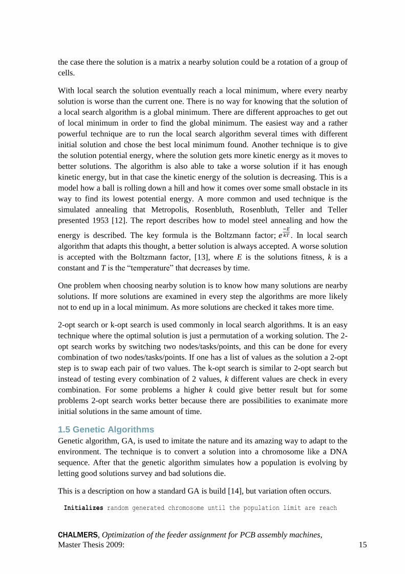
If the same chromosomes as in Figure 10 are used for Ranked Roulette Wheel the wheel
looks like Figure 11. There, the worst chromosome 7 to 10 doesn’t get so much percent
in the ranked roulette wheel and the top solutions get more percent. This approach is
also suited if the chromosomes vary very much. If a chromosome takes up 90% of a
Roulette Wheel in the first method, it will get much lower percent in Ranked Roulette
Wheel so that more diverse chromosomes can be produced.
Equation 1, Ranked Roulette Wheel formula
Roulette Wheel
Chromosome 1
Chromosome 2
Chromosome 3
Chromosome 4
Chromosome 5
Chromosome 6
Chromosome 7
Chromosome 8
Chromosome 9
Chromosome 10
CHALMERS, Optimization of the feeder assignment for PCB assembly machines,
Master Thesis 2009: 18
Figure 11, Ranked Roulette Wheel
Tournament selection is another method of selection. As it is describe in [17] the
chromosome in the current population is competing to be in the mating pool. A number
of chromosomes (usually 2) are selected randomly from the population and the best one
of these is added to a mating pool. The same action is repeated until the mating pool is
full, and then the parents for mating are selected by random from the pool.
1.5.4 Crossover function
The actually breeding is done in the crossover function. How the crossover is done
depends on how the chromosomes are encoded. If the chromosomes are permutations it
is a little bit tricky to get permutations as new chromosomes. If the chromosomes are
not permutations the easiest way to breed new chromosome is the single point
crossover. Take a position by random and for the positions before the random position
take the genes from first parent and for the genes after the random position take the
genes from the second parent. For example if we breed two parents, P1 = {11101101}
and P2 = {01010111} and have the single point at three the new child is C =
{11110111}, but there is also simple to breed a second child as {01001101}. Instead of
a single point crossover, there could be two (or more) point crossover, and for each
point switch between the parents. For example with a 2-point crossover with the prior
parents the result for crossover point at 2 and 5 would be C1 = {11010101} and C2 =
{01101111}. Uniform crossover chooses for each position a gene by random choosing
which parent it will be copied from. This makes it possible for every type of
combinations of two parents to be found. For the single (and more) point crossover
there is a limit. For example the single point crossover could just generate 16 different
outcomes from two parents with 8 genes and the Uniform crossover could generate 256
different outcomes. This number is smaller than the two parents have some genes in
Ranked Roulette Wheel
Chromosome 1
Chromosome 2
Chromosome 3
Chromosome 4
Chromosome 5
Chromosome 6
Chromosome 7
Chromosome 8
Chromosome 9
Chromosome 10

CHALMERS, Optimization of the feeder assignment for PCB assembly machines,
Master Thesis 2009: 19
common. But with Uniform crossover it is more likely that the method destroys a
sequence of genes that are good as a group.
The algorithms above don’t work if the chromosome is a permutation. For example if
P1 = {12345678} and P2 = {345678123} and a single point crossover at position four
the new chromosomes would be C1 = {12348123} and C2 = {34565678}, and this is
not a permutation of the solution. A way to overcome this is the Partially Mapped
Crossover, PMX, describe in Goldberg and Lingle [18]. This is how it works:
Randomly select a span of genes from P1 and copy them directly to the new
chromosome. Note the indexes of the segment
Looking in the same segment positions in P2, select each value that hasn't
already been copied to the child.
For each of these values (a):
(i) Note the index of this value in P2. Locate the value, V, from P1 in this
same position.
Locate this same value in P2
If the index of this value in P2 is part of the original span
Go to step i. using this value.
Else
Insert (a) value into the chromosome in this position.
End for
Copy any remaining positions from P2 to the chromosome.
1.5.5 Mutation
Mutation is sometimes necessary in order to find new chromosomes and nature is using
this. It is a simple step where the new chromosome undergoes a small change. So by
random a small part is changed or swapped.
1.5.6 Survival
The way to choose which chromosomes survive until the next generation can be done in
different ways. One way is that only the two children after each reproduction survive.
But a more effective way is the elitism. It says that the best chromosomes always
survive. So, if the new chromosomes are worst than the parents, the parents are kept in
the population. With the elitism the best (and sometime the optimal) solution is kept to
the end.
1.6 Heuristic
Heuristic is the method to do choices based on experience rather than proof [19]. This
knowledge is based on knowing the problem and the experiment of what works and
don’t. This could be used in chess playing to assume that some opening is better than
other. For solving the feeder assignment problem heuristic way stats that is better to
pack the components in the feeder bank, because that will lower the placement heads
movements.

CHALMERS, Optimization of the feeder assignment for PCB assembly machines,
Master Thesis 2009: 20
2 The Traveling salesman problem transformation
When this problem was investigated and constructed, two different approaches for
transforming the travel salesman problem (TSP) into assembly mounted problem were
found. TSP is known to be a NP-hard problem [20]. The following description proves
that the surface mounted PCB problem is NP-hard in two different aspects.
2.1 General TSP
The TSP problem is an old problem about a salesman’s travel. It is not known when it
was first introduced but there are writings about the problem from the 1800 century
[20]. The problem is to visit n different cities where the distance between the cities are
known and the goal is to minimize the total length to visit every city once and only once
and then back to the starting city.
2.2 Placement TSP
For transforming a TSP problem into a placement problem the revolver capacity is set
to n, so that the revolver has n spindles. Now, locate a feeder slot at the first cities
position, for the rest of the positions set them as a placement position for one particular
part. The assembly problem is now to pick n-1 components in the feeder slot and then
place the components in the different placement positions. If the problem can be solved
optimally in the assembly problem the solution could easily be transformed back as a
solution to the TSP problem. Therefore if it exist a polynomial time algorithm for the
assembly problem, a TSP could be solved in polynomial time, this shows that the
assembly problem is at least as hard as TSP, in other word it is NP-hard.
2.3 Feeder bank assignment
In assembly mount problem, a revolver needs to pick-up components in different feeder
slots and then place them at the PCB. Each component has a required nozzle that needs
to be in the revolver head in order for the revolver to pick up the component.
In order to transform the TSP problem to a feeder bank assignment problem create n
components each with a unique part number and one placement each. Each of the
components has a unique nozzle which means that the revolver head will be populated
with n nozzles. Make the revolver head fixed so that the nozzles in the spindles are
always the same which leads to that the pickup order of the components will be the
same for ever feeder assignment. Create n feeder slots and give the feeder slots the same
positions as the cities. There will therefore be n feeder slots spread out as the cities.
With the assembly cost function there is a small modification. The calculation for the
placements of components will not be included, just the pickups. So the pickup order
and cost is calculated as:
Move head to feeder banks slot for the components which requires the nozzle in
the last spindle head
For every spindle head

CHALMERS, Optimization of the feeder assignment for PCB assembly machines,
Master Thesis 2009: 21
Find feeder slot that have the component that require the nozzle that’s in
the current head
Increase the Cost with the Euclidean 2D distance between previous position
and position for the feeder slot related to current head.
Update position to the current feeder slot
End for loop
With this procedure the cost of a TSP problem is possible to calculate. Each feeder slot
has a component that indicates in which order it will be visit. So instead of a list in
which the cities should be visit (as usually with the TSP) each feeder slot will have a
component (number) which tells in which order it will be visit.
Therefore if an optimal solution is found in the feeder bank assignment problem the
result can be transformed back to a TSP solution. The assignment problem is NP-hard
because it is as hard as TSP to solve.

CHALMERS, Optimization of the feeder assignment for PCB assembly machines,
Master Thesis 2009: 22
3 Methods
The algorithms for feeder assignment problem are compared by making a set of
experimental tests. These tests follow the flow of Figure 12.
Figure 12, Flow of the experimental tests
The first four steps are done in the new proposed optimizing program and the last three
steps are preformed in the existing software from Valor. The whole test procedure is
scripted in Valor’s software but the actually feeder optimizing is done thru a binary file
outside Valor’s software. This test procedure of the system model is repeated for every
setting of the parameter.
3.1 Internal structure
The model of the problem instances consists of three blocks / classes. The
MachineConfiguration model contains all the information needed to describe a machine.
Second the PCB model describes the PCBs. Third the Optimizing is a class that is
inherited by each algorithm. Figure 14 shows how the MachineConfiguration is
modeled. MachineConfiguration is the main class that implements a machine having a
number of NozzleBanks, Revolvers and FeederBanks, each with its own attributes.
MachineConfiguration contains the information on how to populate the feeder banks for
Valor’s software.
Import Valor Machine data and
PCB setup
Choose the feeder assignment
algorithm and its parameters
Optimize the feeder assignment according to the
cost function
Write feeder assignment into
setup file
Load Setup file into Valor's
software
Optimize placement order
Write the total production time
into file

CHALMERS, Optimization of the feeder assignment for PCB assembly machines,
Master Thesis 2009: 23
Figure 14, MachineConfiguration class.
The PCB structure is described in Figure 13. A PCB has several components and each
of them is of a specified Part type. Each component can be described as a placement and
all components have a RefDes, Reference Description, which is the unique name for its
placement. This description is sometimes printed in text on the PCB. The algorithms are
build around an Optimizer class from where they inherit functions and also overload the
optimize function, see Figure 15. Each algorithm is loaded with a
MachineConfiguration for description the setup to optimize. If a certain part already has
been placed in the feeder slots or the revolver head is populated, this is considered by
the proposed algorithms. After the optimization is done the results are exported. Except
for these classes there is also a data structure that records static relations and lookup
tables. That data structure states what type of nozzle each part needs to be picked with,
what kind of feeder group a part is stored in and also some other look up tables for
speeding up the optimization. The cost function has its own class for calculating the
feeder assignment cost. The cost function takes a MachineConfiguration as parameter
and calculated the cost for determinate how well a solution is. How the cost is
calculated is described below.
Figure 13, PCB class
1 *
1*
+Name
+Profile
PCB+Location : Position
+Angle
+RefDes
Component
+IPN : TPart
Part
* 1
*1
1 * 1 *
1 ** 1
*
1
* 1
+Import()
+Export()
+Name : String
+TablePosition : Position
+TableHeigth : Integer
+TableWidth : Integer
+Camers : Position
MachineConfiguration
+Name : String
NozzleBank+Nozzle : TNozzle
+Location : Position
+Name : String
NozzleBankSlot
+Name : String
FeederBank+Name : String
+PickTime : Integer
+PlacementTime : Integer
+MovementTime : Integer
Revolver +Location : Position
+Width : Integer
+Feeder : String
+FeederGroup : String
+Name : String
+ComponentCapacity : Integer
+Fixed : Boolean
FeederSlot
-Nozzle : String
-Count
AvailableNozzle
+Nozzle : TNozzle
+Name : String
Spindle
+IPN : TPart
Parts
*
1
*
1

CHALMERS, Optimization of the feeder assignment for PCB assembly machines,
Master Thesis 2009: 24
3.2 Time factors
As mention in the introduction, there are several time factors in an assembly machine
model to consider. This is a list of known time factors.
Loading of the bare PCB
Head movements
Recognition of the fiducial marks
Component Pick-up
Component Checking
Component Placements
Change time for nozzles
In the model of this thesis there are some simplifications, but the core thoughts
originates from Kallio et al. [21] on a realistic simulator of placement machines.
Loading of the PCB and the recognitions of fiducial marks are not considered as this is
the same operation for every setup. The total production time for a machine setup is
given by Equation 2. Here we recognize that the slowest revolver is the bottleneck of
the
Equation 2, Total time
production time. For the calculation of time used by a revolver head, let G be the
number of task blocks, number of times the revolver goes from picking components in
feeder bank to placing components on the PCB, CCj the time for picking components
Equation 3, Time for a revolver
+Optimize() : MachineConfiguration
+LoadMachineConfiguration(in MachineConfig : MachineConfiguration)
+LoadPCB(in PCB : PCB)
Optimizer
+Optimize() : BankConfiguration
Algorithm1
+Optimize() : BankConfiguration
Algorithm2
Figure 15, Algorithms classes

CHALMERS, Optimization of the feeder assignment for PCB assembly machines,
Master Thesis 2009: 25
for task block j, and CPj the time of placing components for task block j. Then, the time
for each revolver can be calculated as Equation 3. CCj can be given as Equation 4 where
A is number of components to place, MPij is the time to move to the pickup position of
component i in task block j and Pij is the pick-up time for component i in task block j.
CPj can be describe as Equation 5 where A is number of components to place, MIij is the
movement time to the placement position for component i of task block j and Iij is the
placement time for component i in task block j.
Equation 4, Pick-up phase
Equation 5, Placement phase
3.3 Cost function for evaluating feeder assignments
The quality of the feeder assignment is evaluated by a cost function. As the main focus
of this thesis is the solution of the feeder assignment problem the cost function looks on
that part of the PCB assembly problem. Therefore the cost function considers the feeder
setup, the settings of the revolver heads and the PCB and calculates a cost for it. The
cost function does not suppose that the placement problem has been solved optimally.
In contrast to that a greedy approach is used. This simple procedure creates a placement
order and then calculates the cost for it using the time functions mention above. The
reason to trust on a greedy approach for placement order is sufficient due to the simple
nature of the cost function. The procedure for evaluating the cost is described as the
following pseudo-code and is called S.
ComponentToPlace = Number of components to place for revolver
Cost = 0
CurrentPosition = Center of PCB
While ComponentToPlace is greater than zero
For every spindle in Revolver
If first spindle then
F = Component, with matching nozzle as spindle, in feeder bank with most
placements left
Else
F = Closest feeder bank with matching nozzle between spindle and component
End if
Increase Cost with movement time from CurrentPosition to feeder slot F

CHALMERS, Optimization of the feeder assignment for PCB assembly machines,
Master Thesis 2009: 26
Increase Cost with pick-up time for component in F
Increase Cost with placement time for component in F
Increase Cost with an average time for moving between placements
Update CurrentPosition to feeder slot F.
Decrease ComponentToPlace
End for
If revolver needs to verify some components in a camera station
Increase Cost with movement to camera Station
Update CurrentPosition to camera station
End if
Increase Cost with movement to average position for component in the first
Nozzle
Update CurrentPosition to average position for component
Increase Cost with movement to center of PCB
Update CurrentPosition to center of PCB
End while
As can be seen there is no consideration of the placement position in S except for the
first component in every task block. This is because the placements can be done in
many different ways and therefore that sequence is excluded. The average time for
moving between placements is analyzed by Valor’s software using several different
PCB job.
The time for placements head movements is determinate by the longest axial distance,
because the head moves independently in the x- and y-directions. The time in
millisecond for the particular machine is the distance in millimeters times 0.5 plus 132.
This has been verified from the movement graphs given by Valor, it is not a perfect
match but close in the general case.
For evaluating the performance of the algorithms in solving the TSP problems an
optimized version of the cost function was developed, named STSP. It is almost the
same as the previous cost function, S, but there are some simplifications and the
distance calculation are modified to reflect the TSP. The pick-up order in procedure
STSP is same as procedure S for TSP problems. The cost is calculated as this:
Find component that needs the nozzle for the last spindle in revolver
Set CurrentPosition to that component’s feeder slot
Set Cost to zero
For every spindle in head
Find component that needs the nozzle for current spindle
Set F to feeder slot for that component
Increase Cost with Euc2D between CurrentPosition and F
Update CurrentPosition to F
End for

CHALMERS, Optimization of the feeder assignment for PCB assembly machines,
Master Thesis 2009: 27
Distance between positions is calculated with Euclidean distance function for 2D, which
is based on Pythagorean formula, which is used in
general TSP problems.
3.4 Revolver setup
How to populate the revolver head with nozzles in an optimal way is a hard problem,
because this depends on two NP-hard problems, the placement problem and the feeder
assignment problem. The task in this thesis is to evaluate the performance of our
proposed algorithm in Valor’s software. Therefore, the nozzle to head assignment
technique that is used in this thesis is the same as in Valor’s software. The technique
aims at minimizing the number of task blocks. The algorithm works in following ways:
Populate revolver with one nozzle of each type that is needed for placing the
components
While space left in revolver
Find nozzle with highest ratio, placements with that nozzle / nozzles of that
type already in revolver
If two or more nozzle has the same ratio choose the one with the most
placements
Add that nozzle to Revolver
Decrease space left in revolver
End while
Sort revolver by first nozzle type count and second nozzle name
For an example, if a revolver with 10 spindles should place 12 components with nozzle
A and 5 components with nozzle B and 7 components with nozzle C and 1 component
with nozzle D the revolver will look like this; 4 of A, 3 of C, 2 of B, 1 of C.
This algorithm does not guarantee the finding an optimal placement order. It is said that
it will minimize the number of task blocks to the optimal but this has not been proven.
3.5 Algorithms
Three different algorithms have been developed for solving the feeder assignment
problem and also a variation of two of them is tested. The first algorithm is a simple
randomized setup algorithm with heuristics, the second applies local search technique
and the last one is a genetic algorithm. In order to do a fair comparison of the
algorithms, they are run for a limited period of time. This will be achieved by adjusting
the number of generations and the number of new starts.
3.5.1 Randomized
The algorithm consist of a loop to generate a randomized feeder assignment and then
the feeder banks are packed, meaning that every component is moved towards the center
of the feeder bank so that no spaces exist between the components. After that the cost

CHALMERS, Optimization of the feeder assignment for PCB assembly machines,
Master Thesis 2009: 28
for the feeder setup is calculated and the best solution is kept. See Appendix 1 for
pseudo-code.
3.5.2 Local Search
Local search is performed in a straight forward manner. The neighborhood is rather
large; swapping of each pair of feeder slots is tested. If a better solution is found it is
kept and the same is iterated until no more single swaps produce a better solution. After
that the local search is restarted from a new randomized feeder setup. The algorithm is
terminated when the given time limit of the running time is reach. A pseudo-code of the
algorithm can be found in Appendix 1. An extended version of local search was also
developed, it has the same basic idea as the ordinary local search but after no
improvement could be found by swaps, the algorithm tries to invert the order of the
components of a group of feeder slots. For an example if we have components in the
order <1,2,3,4,5,6,7,8> and we invert the order of components from position 2 to 5 the
result should be <1,5,4,3,2,6,7,8>. This operation is done for every position and the
length from two to the end of feeder bank.
3.5.3 Genetic Algorithm
The genetic algorithm applies the PMX crossover and ranked roulette wheel selection
method. The mutation step consists of randomized swapping of components. One
problem that was discovered with an ordinary PMX is that it could not handle the
situation where several parts can be stored in the same feeder slot. Therefore a
modification of PMX was developed, see Appendix 1. The idea is to use the PMX
crossover method and if this creates conflicts they are postponed and solved later. The
Uniform crossover method was also tested as a second version. The Genetic Algorithms
are run with a population of 100 and with 80 children. The mutation rate is set to 5%.
3.6 Lower bound
For knowing how well the results are, a lower bound algorithm has been developed. The
goal was to produce a lower bound function that gives as high value as possible. Let n
be the number of components to place, pp the time to rotate revolver head one step plus
the minimum time to place a component, t the number of needed task blocks, c the
closest distance between a feeder slot and the center of board, r the number of revolver
heads and m the number of placements for the part that have most placements. Then the
lower bound can be calculated as in Equation 6.
Equation 6, Lower bound
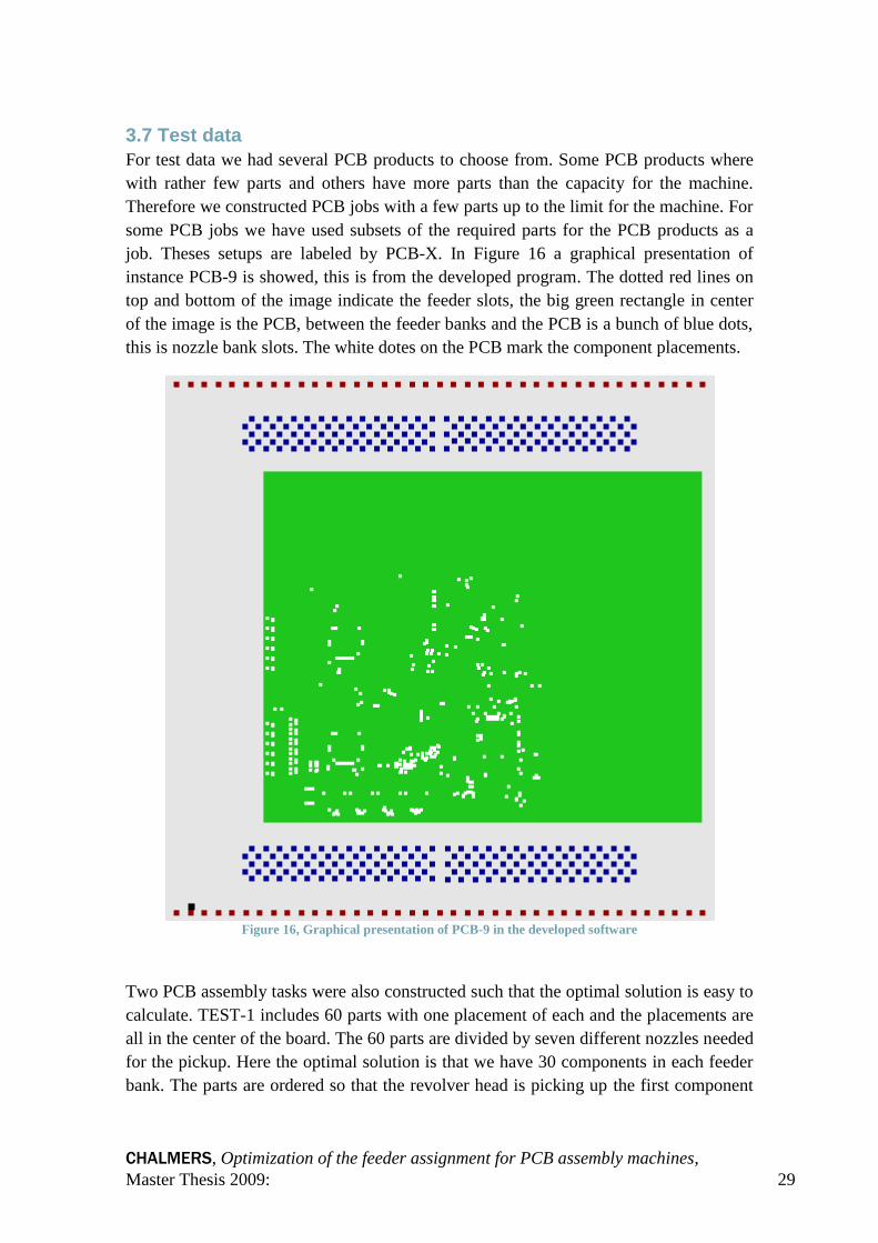
CHALMERS, Optimization of the feeder assignment for PCB assembly machines,
Master Thesis 2009: 29
3.7 Test data
For test data we had several PCB products to choose from. Some PCB products where
with rather few parts and others have more parts than the capacity for the machine.
Therefore we constructed PCB jobs with a few parts up to the limit for the machine. For
some PCB jobs we have used subsets of the required parts for the PCB products as a
job. Theses setups are labeled by PCB-X. In Figure 16 a graphical presentation of
instance PCB-9 is showed, this is from the developed program. The dotted red lines on
top and bottom of the image indicate the feeder slots, the big green rectangle in center
of the image is the PCB, between the feeder banks and the PCB is a bunch of blue dots,
this is nozzle bank slots. The white dotes on the PCB mark the component placements.
Figure 16, Graphical presentation of PCB-9 in the developed software
Two PCB assembly tasks were also constructed such that the optimal solution is easy to
calculate. TEST-1 includes 60 parts with one placement of each and the placements are
all in the center of the board. The 60 parts are divided by seven different nozzles needed
for the pickup. Here the optimal solution is that we have 30 components in each feeder
bank. The parts are ordered so that the revolver head is picking up the first component
CHALMERS, Optimization of the feeder assignment for PCB assembly machines,
Master Thesis 2009: 30
in slot one and the second component is picked up in slot two and so on. Is means that
the revolver goes to the feeder bank and do a straight line move over the feeder bank
and then go to the placements in the middle of the board. TEST-2 consists of 11 parts
with a total of 240 placements. The optimal solutions is such that 5 parts are in one
feeder bank and 6 parts in the other and each revolver head has 120 placements and they
are done in exactly four task blocks.
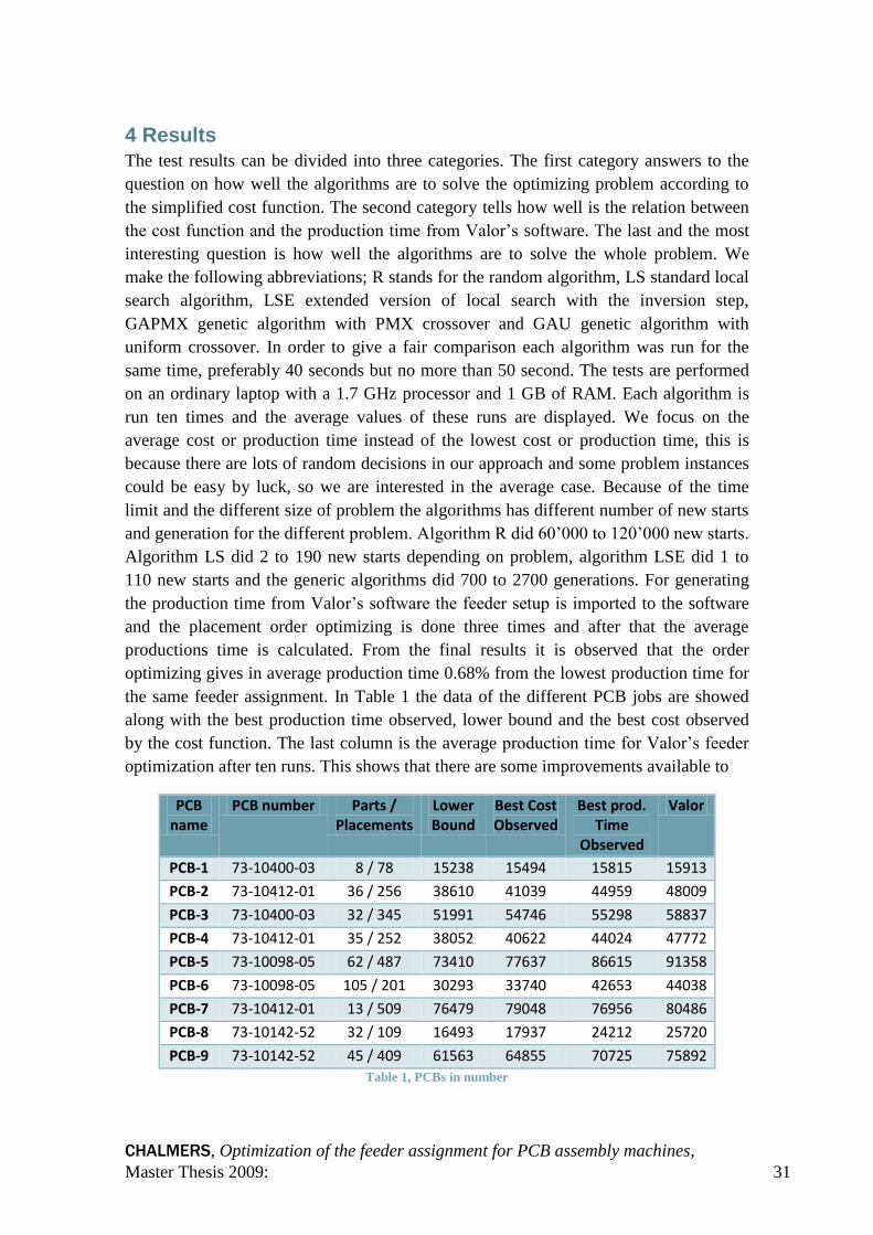
CHALMERS, Optimization of the feeder assignment for PCB assembly machines,
Master Thesis 2009: 31
4 Results
The test results can be divided into three categories. The first category answers to the
question on how well the algorithms are to solve the optimizing problem according to
the simplified cost function. The second category tells how well is the relation between
the cost function and the production time from Valor’s software. The last and the most
interesting question is how well the algorithms are to solve the whole problem. We
make the following abbreviations; R stands for the random algorithm, LS standard local
search algorithm, LSE extended version of local search with the inversion step,
GAPMX genetic algorithm with PMX crossover and GAU genetic algorithm with
uniform crossover. In order to give a fair comparison each algorithm was run for the
same time, preferably 40 seconds but no more than 50 second. The tests are performed
on an ordinary laptop with a 1.7 GHz processor and 1 GB of RAM. Each algorithm is
run ten times and the average values of these runs are displayed. We focus on the
average cost or production time instead of the lowest cost or production time, this is
because there are lots of random decisions in our approach and some problem instances
could be easy by luck, so we are interested in the average case. Because of the time
limit and the different size of problem the algorithms has different number of new starts
and generation for the different problem. Algorithm R did 60’000 to 120’000 new starts.
Algorithm LS did 2 to 190 new starts depending on problem, algorithm LSE did 1 to
110 new starts and the generic algorithms did 700 to 2700 generations. For generating
the production time from Valor’s software the feeder setup is imported to the software
and the placement order optimizing is done three times and after that the average
productions time is calculated. From the final results it is observed that the order
optimizing gives in average production time 0.68% from the lowest production time for
the same feeder assignment. In Table 1 the data of the different PCB jobs are showed
along with the best production time observed, lower bound and the best cost observed
by the cost function. The last column is the average production time for Valor’s feeder
optimization after ten runs. This shows that there are some improvements available to
PCB name
PCB number Parts / Placements
Lower Bound
Best Cost Observed
Best prod. Time
Observed
Valor
PCB-1 73-10400-03 8 / 78 15238 15494 15815 15913
PCB-2 73-10412-01 36 / 256 38610 41039 44959 48009
PCB-3 73-10400-03 32 / 345 51991 54746 55298 58837
PCB-4 73-10412-01 35 / 252 38052 40622 44024 47772
PCB-5 73-10098-05 62 / 487 73410 77637 86615 91358
PCB-6 73-10098-05 105 / 201 30293 33740 42653 44038
PCB-7 73-10412-01 13 / 509 76479 79048 76956 80486
PCB-8 73-10142-52 32 / 109 16493 17937 24212 25720
PCB-9 73-10142-52 45 / 409 61563 64855 70725 75892
Table 1, PCBs in number

CHALMERS, Optimization of the feeder assignment for PCB assembly machines,
Master Thesis 2009: 32
do for Valor’s software. The improvements that can be done are from 0.62% to 7.85%
with an average of 5%.
4.1 Performance of the algorithms subject to the cost function
Table 2 shows the results of the TEST runs. The results are given as percentage from
the known optimal solution using procedure S. TEST-1f and TEST-2f is the same as
TEST-1 and TEST-2 but here the revolver is fixed to the nozzle that is used in the
optimal solution. Here we can observe that the algorithms don’t have any problems to
find the optimal solution for the setup with just a few parts but with lots of placements.
The optimal solution has been compared also to the lower bound. For TEST-1 the
algorithms showed worse performance in finding good solutions. For TEST-1 the
optimal solution is 28.47 % higher than the lower bound and for TEST-2 the optimal
solution is 7.28 % higher than the lower bound.
R LS LSE GAPMX GAU
TEST-1 3,52 % 0,00 % 0,00 % 1,12 % 1,46 %
TEST-2 0,14 % 0,00 % 0,00 % 0,08 % 0,20 %
TEST-1f 6,80 % 8,24 % 6,92 % 3,31 % 4,08 %
TEST-2f 0,16 % 0,00 % 0,00 % 0,02 % 0,03 %
Table 2, TEST results with procedure S
The performance in solving the PCB jobs of the algorithms of the present studies is
compared to each other in Table 3. The optimal solution is not known here. The percent
ratio is compared to the best algorithm. The last column in Table 3 is the ratio between
the best solution observed and the lower bound. It turns out that the different algorithms
PCB R LS LSE GAPMX GAU Best
PCB-1 0,00 % 0,00 % 0,00 % 0,00 % 0,00 % 1,68 %
PCB-2 1,47 % 0,75 % 0,64 % 0,35 % 0,00 % 6,29 %
PCB-3 0,79 % 0,33 % 0,39 % 0,00 % 0,04 % 5,30 %
PCB-4 1,23 % 0,39 % 0,40 % 0,38 % 0,00 % 6,75 %
PCB-5 1,94 % 0,67 % 0,50 % 0,11 % 0,00 % 5,76 %
PCB-6 3,71 % 0,42 % 0,00 % 0,15 % 1,59 % 11,38 %
PCB-7 0,00 % 0,06 % 0,16 % 0,23 % 0,21 % 3,36 %
PCB-8 0,85 % 0,28 % 0,12 % 0,37 % 0,00 % 8,76 %
PCB-9 1,21 % 0,34 % 0,19 % 0,09 % 0,00 % 5,35 %
Average 1,24 % 0,36 % 0,27 % 0,19 % 0,21 %
Table 3, PCB results with procedure S

CHALMERS, Optimization of the feeder assignment for PCB assembly machines,
Master Thesis 2009: 33
are almost equal in producing good result except for R. For PCB-1 an exhaustive search
was done and the best solution found by the algorithms is also the optimal solution
subject to cost function. The performance of the algorithms to solve the TSP problem
for feeder bank assignment problem with procedure STSP was also tested, see Table 4.
Problem instances r4 and r11 are small TSP problems with 4 and 11 cities placed by
random and the optimal solution is calculated by testing every combination. Problem
instance wi29, dj28, xqf131 has been taken directly from Georgia Tech’s TSP
homepage [22] where the optimal solution is known.
R LS LSE GAPMX GAU
r4 0,00 % 0,00 % 0,00 % 0,00 % 0,00 %
r11 2,65 % 0,00 % 0,00 % 0,00 % 0,00 %
wi29 134,70 % 5,25 % 5,23 % 9,89 % 8,27 %
dj38 191,27 % 22,21 % 28,16 % 33,42 % 19,71 %
xqf131 581,66 % 97,48 % 104,90 % 399,02 % 247,94 % Table 4, TSP problem results
4.2 Relation between cost function and production time
In Figure 17 results of all test runs for all the algorithms are displayed using the cost
from procedure S in the y-axis and the actual production time from Valor’s software in
x-axis. The groups of dots are the repeated runs for each PCB job. The straight line is
the trend line regression for the result. The relation is almost linear and not far away
from a 1:1 match. One thing to mention is that the loading of PCB is not a part of the
procedure S and this is typically of the size 2500 milliseconds. In the case with PCB-1
(Figure 18) we can see that the actual production time can vary up to 423 milliseconds
for the same cost calculated by procedure S. As mention earlier it has been observed
that the average difference in production times is 0.68% for the same feeder assignment.
In the worst case it has been observed that the production time could differ 7.5% from
the best production time to the worst case for the exactly same feeder assignment. The
average different in production time for ten runs compared to the lowest production
time found in the ten runs for each PCB is summarized in Table 5
PCB-1 PCB-2 PCB-3 PCB-4 PCB-5 PCB-6 PCB-7 PCB-8 PCB-9
0,22 % 0,68 % 0,61 % 0,90 % 0,80 % 1,00 % 0,48 % 0,49 % 0,98 % Table 5, Average difference in production time for exact same feeder assignment
The production time is therefore not treated as a fixed value instead it is an indication of
how well the final production time can be after the placements order has been solved.
For PCB-2 (Figure 19) and PCB-5 (Figure 20) it is observed that the trend line is not as
good as in Figure 17, and the line is almost horizontal for PCB-2. Two interesting
observation can be done from the figures; the instance which gives the lowest cost

CHALMERS, Optimization of the feeder assignment for PCB assembly machines,
Master Thesis 2009: 34
according to procedure S also gives the lowest production time. For PCB-8 (Figure 21)
the trend line points in the right direction but the relation between the cost function
result and the production time is not perfect. The instance that gives the lowest cost, by
procedure S, gives not the lowest production time neither is it in the top ten production
time and the best production time is not in the top ten instances with lowest cost by
procedure S.
Figure 17, Relation between procedure S and production time for all PCBs
0
10000
20000
30000
40000
50000
60000
70000
80000
90000
100000
0 10000 20000 30000 40000 50000 60000 70000 80000 90000 100000
Co
st b
y p
roce
du
re S
Production Time Valor's software (ms)
All PCBs
Linear (All PCBs)

CHALMERS, Optimization of the feeder assignment for PCB assembly machines,
Master Thesis 2009: 35
Figure 18, Relation between procedure S and production time for PCB-1
Figure 19, Relation between procedure S and production time for PCB-2
15300
15350
15400
15450
15500
15550
15600
15650
15700
15900 15950 16000 16050 16100 16150 16200 16250 16300
Co
st b
y p
roce
du
re S
Production Time Valor's software (ms)
PCB-1
Linear (PCB-1)
39000
39500
40000
40500
41000
41500
42000
42500
43000
43500
44000
45000 45500 46000 46500 47000 47500 48000 48500 49000 49500 50000
Co
st b
y p
ro
ced
ure S
Production Time Valor's software (ms)
PCB-2
Linear (PCB-2)

CHALMERS, Optimization of the feeder assignment for PCB assembly machines,
Master Thesis 2009: 36
Figure 20, Relation between procedure S and production time for PCB-5
Figure 21, Relation between procedure S and production time for PCB-8
74000
75000
76000
77000
78000
79000
80000
81000
82000
86000 87000 88000 89000 90000 91000 92000 93000 94000
Co
st b
y p
ro
ced
ure S
Production Time Valor's software (ms)
PCB-5
Linear (PCB-5)
16000
16500
17000
17500
18000
18500
19000
24000 24500 25000 25500 26000 26500 27000
Co
st b
y p
ro
ced
ure S
Production Time Valor's software (ms)
PCB-8
Linear (PCB-8)

CHALMERS, Optimization of the feeder assignment for PCB assembly machines,
Master Thesis 2009: 37
4.3 Performance of the algorithms to solve the whole problem
The performance of the algorithms is summarized in Table 6. Here we can see how well
the feeder assignments actually are in the real production after the placement order
optimizations has been done. Each algorithm is compare to the result of Valor’s feeder
optimization. The production time for Valor’s software is the average production time
after ten runs of feeder optimization from a random start and the placements order
optimization. As can been seen in the table, every algorithm manage to get better
production times than Valor’s software. The best algorithm in an average turns out to be
the genetic algorithm with Uniform crossover but it is not the best algorithm for every
PCB jobs. The results differ a lot between different PCB jobs. Some PCB jobs gets up
to 3.5 percent improvements against Valor’s optimization but some other will have just
under a percents improvement and for the first PCB job the results are even worse. The
best algorithm is only slightly better than the others. Interested things are that the next
best algorithm is the random based algorithm, because it operates very badly in the task
to find the lowest cost by procedure S.
PCB Valor R LS LSE GAPMX GAU
PCB-1 100,00 % 101,62 % 101,39 % 101,31 % 101,09 % 100,98 %
PCB-2 100,00 % 97,29 % 98,67 % 98,47 % 98,84 % 96,92 %
PCB-3 100,00 % 97,25 % 99,42 % 99,97 % 98,46 % 97,67 %
PCB-4 100,00 % 97,22 % 96,93 % 97,64 % 96,42 % 97,08 %
PCB-5 100,00 % 98,89 % 99,47 % 98,73 % 98,31 % 97,64 %
PCB-6 100,00 % 100,73 % 99,67 % 100,71 % 100,93 % 100,82 %
PCB-7 100,00 % 97,18 % 97,52 % 97,93 % 97,90 % 98,27 %
PCB-8 100,00 % 98,92 % 99,04 % 99,10 % 100,04 % 99,39 %
PCB-9 100,00 % 99,88 % 98,15 % 98,46 % 98,91 % 96,50 %
Average 100,00 % 98,78 % 98,92 % 99,15 % 98,99 % 98,36 % Table 6, Performance of the algorithms solving the final problem

CHALMERS, Optimization of the feeder assignment for PCB assembly machines,
Master Thesis 2009: 38
5 Discussion
The first step for this thesis was to develop a machine model software where it is
possible to import, optimize and export the results to Valor’s software. This has been
working well with some minor problems that have been solved. It has also been shown
that there are improvements to be done in Valor’s software and some more production
seconds to earn. In the task for solving the problem subject to the cost function the
algorithm had different success rates. For constructed problems and the PCB job where
the optimal solution could be calculated, the proposed algorithms of the present work
found the optimal solution for the most cases, as seen in Table 2. For TEST-1 where we
have 60 parts in every feeder bank the task is more complicated and it is almost to solve
two TSP problem with 30 cities. This is not all true because we don’t have unique
nozzle need for each part, therefore some parts can swap places and we still have an
optimal solution, this is not possible for TSP. TEST-2 is an simpler problem to solve as
we have fewer components to place in the feeder banks. For TEST-1f the algorithms
have more difficulties to find the optimal solution. One theory why this happens is
because the nozzles are fixed in the revolver head some solution have a greater number
of task blocks than if the nozzles were repopulated in the revolver head for each feeder
assignment in order to minimize the task blocks. This leads to more local minima and
local search algorithms have more difficulties than GA to get out of local minima and
find the global minimum.
The algorithms performance, Table 3, to find good solutions where the optimal solution
is unknown is not so diverted. The algorithms are equally good but the random based
algorithm somewhat worse. GA solves the task better than LS but the difference is too
small in order to say some conclusions from that. For the most PCB jobs and in special
for PCB-7 the best solution is not far away from the lower bound. The algorithms solve
the task well and produce solutions near optimal solution or the optimal solution for the
feeder assignment problem subject to the cost function. One factor that affects the
solution is the running time for the algorithm. We have chosen a rather short running
time because industry manufactures work daily with planning PCB production and they
can’t wait on the computer for long time. The randomized based algorithm gives not
much better results by increasing their running time. As it is now the randomized based
algorithm checks around 80 000 feeder assignments in 40 seconds. If the time is double
so that 80 000 more feeder assignments are checked the probability to find a better
solution then is found so far is not high. But for the genetic algorithm is takes a longer
time before the population converts to a good solution and its results improve then the
running time is increased.
In the case of the TSP relaxation problem the algorithm has big difficulties for bigger
problem instances. It founds the optimal solution for smaller problems but the bigger
ones the results are not good. The theory is that the LS has difficulties to find a good
solution as the relaxation of the problem makes the 2-opt step work in a different way.
CHALMERS, Optimization of the feeder assignment for PCB assembly machines,
Master Thesis 2009: 39
Also the relaxations of the problem produces lots of local minima. LS has been proven
to work well for TSP problems only when the starting setup has some potential.
The cost function that has been developed in this thesis has been proven to work well.
We have an almost 1:1 relation when considered all the PCBs. But it is not as good for
the last percentage from optimal solution. This can be seen in Figure 18 to Figure 21.
For the case with PCB-1 it is clear that the cost function fails to model the small
difference in the production time caused by the changes in the feeder assignment. Two
hypotheses why these errors occur success themselves. The first is that the simplified
placement order has not been good. The actual placements order differs much from the
simplified. The information of the actual placements is not considered in model. The
second hypothesis is that the cost function is omits some important time factors that
affects the production time. However, if we look the best solutions found by our
optimizer their real production time may be worse than those of some other not as good
solutions. This mirrors in accuracy of our model.
One problem in generating placement order is the big variation of the production time,
because one feeder assignment could give results that differ up to 7%. Therefore it is
important that the placement order optimization is run several times in order to find the
best solution when the product is used in real industrial production environment.
It was observed the approach of the present study that (splitting the problem and
applying well known algorithm) produces better solutions than the industrial solution.
The approach has lowered the production time by 1.67% with GAU. It also showed up
that there is more space to explore the solution method for revolver head machines and
in this way lowers the production time. With a better algorithm and cost function there
is a possibility to lower the production time to 5% below current average production
time in Valor’s software. It was also shown that even though GA with PMX crossover
solved the optimizing problem subject to the cost function equally well as with Uniform
crossover, the feeder setup from GAU had better feeder assignment structures that allow
better placement orders and production times. The random based algorithm was the
second best algorithm according to the production time and this algorithm does not need
a tuning or local search step. Therefore, solutions from this algorithm have more parts
by random and are not tuned for matching the cost function. Because of this, one can
draw conclusion that the cost function is not perfect for the placement order because the
random algorithm sometime beats the local search algorithm.
CHALMERS, Optimization of the feeder assignment for PCB assembly machines,
Master Thesis 2009: 40
6 Conclusions
This thesis has proposed and evaluated different algorithms and heuristics for the feeder
assignment problem. The results show that the algorithms are capable to produce good
results that are near optimal subject to the cost function. The algorithms also found
solutions that are better than the exiting algorithm in Valor’s software. The algorithms
are almost equally well to solve the task compared to each other. The random based
algorithm is a little bite worse than the others but the inaccurately of the cost function
makes the final results similar. The crossover function for the genetic algorithm affects
the algorithms performance and for this model the Uniform crossover gives slightly
better results.
The expected improvements in the local search algorithm for extending the
neighborhood didn’t appear. In the end it didn’t matter too much which algorithm one
used, they all give almost the same result. Therefore, the task to get better production
times is to improve the cost function. This approach with the current cost function gives
a slightly better result than Valor’s software but as has been seen previous the
improvements could be around 5%.
How big the real improvements are on the production floor is hard to predict, because
the placement order optimization solve the problem with some percentage difference.
Further, the production simulation that is used in Valor’s software also has some
percentage difference to the real production time by the machine. Therefore it is not
possible to say that the production is improved in the factories.
CHALMERS, Optimization of the feeder assignment for PCB assembly machines,
Master Thesis 2009: 41
7 Future Work
As mention earlier the cost function needs more research. Is it possible to define a good
cost function without solving the placement ordering or is it possible to solve the
placement order in the same procedure as solving the feeder assignment problem? One
interested idea is to solve the placement order problem first with all parts pickup
position in the middle of the feeder bank and then after the placement order has been
solved to spread the parts out in the feeder bank. The placement order affects the final
production time and it omission will never give good solution. Therefore this part needs
to be understood and researched more.
The pick-up time in feeder slots, the rotating of revolver head and preparing a new
component in the feeder slot are sometimes done simultaneously in a machine. This and
other complex movements need to be modeled more exactly in order to improve the
cost function.
For the local search algorithm it has been proven that they are affected by the initial
solution. Therefore a future work is to come up with a good initial solution to the feeder
assignment problem.
Future work with heuristic algorithms can involve a doing some more precalculations
on where the parts should be in the feeder banks. Instead of just packing the
components also move them as a group up and down the feeder bank.
The generic algorithms have been tested with implementation of a local search step, but
this has not showed better results. Therefore future work would be to improve and
research on how to implement local search steps to the generic algorithms for better
results.

CHALMERS, Optimization of the feeder assignment for PCB assembly machines,
Master Thesis 2009: 42
8 References
1. Volgenant, A and de Waal, A. A heuristic for multiple-feeder PCB manufacturing.
s.l. : Journal of the Operational Research Society 57, pp. 1134–1141, 2006.
2. Grunow, M, et al. Operations planning for collect-and-place machines in PCB
assembly. s.l. : Computers & Industrial Engineering 47, pp 409–429, 2004.
3. Ayob, M, Cowling, P and Kendal, G. Optimisation for Surface Mount Placement
Machines. s.l. : Proceedings of the IEEE ICIT’02, Bangkok, 11-14 Dec, pp 498-503, ,
2002.
4. Leipälä, Timo, Johnsson, Mika and Nevalainen, Olli. Determining the Manual
Setting Order ofComponent on PCB Boards. s.l. : Journal of Manufactoring Systems
Vol. 15 / No. 3 pp 155-163, 1996.
5. Ayob, Masri. Optimization of Surface Mount Device Placement Machine in Printed
Circuit Board Assembly. s.l. : University of Nottingham, 2005.
6. Johnsson, M and Smed, J. Observations on PCB Assembly Optimization. s.l. :
Electronic Packaging & Production, Vol. 41, No. 5, pp. 38–42, 2001.
7. Smed, Jouni, et al. Job Grouping Surface Mounted Component Printing. s.l. :
Robotics and Computer Integrated Manufacturing, Vol 15, No. 1, pp 39-49, 1999.
8. Johnsson, Mika. Operational and tactical level optimization in printed circuit board
assembly. s.l. : Turku Center for Computer Science, 1999.
9. Valor Computerized Systems. Valor Computerized Systems. [Online]
http://www.valor.com.
10. Universial Instruments. Genesis Platform. [Online] [Cited: September 2, 2009.]
http://www3.uic.com/wcms/WCMS2.nsf/index/Products_17.html.
11. Kleinberg, Jon and Tardos, Éva. Algorithm Design. s.l. : Pearson Education Inc,
pp 661-671, 2006.
12. Metropolis, N., et al. Equation os state calculations by fast computing machines.
s.l. : J. Chem. Phys. 21, 1087-1092, 1953.
13. Kittel, Charles and Kroemer, Herbert. Thermal Physics, 2nd ed. s.l. : Freeman &
Co.: New York, 1980.
14. Mitchell, Tom M. Machine learning. s.l. : McGraw Hill, 1997.
15. Holland, J.H. Adaptation in natural and artigicial systems. s.l. : University of
Michigan Press, 1975.

CHALMERS, Optimization of the feeder assignment for PCB assembly machines,
Master Thesis 2009: 43
16. Ho, W. and Ji, P. A genetic algorithm to optimise the component placement
process. s.l. : Int J Adv Manuf Technol, pp 1397–1401, 2005.
17. Yang, Jiaping and Soh, Chee Kiong. Structural Optimization by Genetic
Algorithms with Tournament Selection. s.l. : Journal of computing in civil engineering,
pp 195-200, 1997.
18. Goldberg, D.E. and Lingle, R. Alleles, Loci, and the Traveling Salesman Problem.
s.l. : Proc. of the 1st Int. Conf. on Genetic Algorithms, pp 154-159, 1985.
19. Janlert, Lars-Erik. Nationalencyklopedin. [Online] [Cited: September 7, 2009.]
http://www.ne.se/lang/heuristik.
20. Schrijver, Alexander. On the history of combinatorial optimization (till 1960).
Handbook of Discrete Optimization, pp 1-68. 2005.
21. Kallio, Kai. Joustavan ladontakoneen suoritusajan arvioinnista. s.l. : Turun
Yliopisto, 2008.
22. Office of Naval Research, National Science Foundation and Georgia Tech.
Traveling Salesman Problem. [Online] School of Industrial and Systems Engineering at
Georgia Tech, August 8, 1991. http://www.tsp.gatech.edu.

CHALMERS, Optimization of the feeder assignment for PCB assembly machines,
Master Thesis 2009: 44
Appendix 1: Algorithms
Randomized algorithm
Set BestSolution to
While time left
Create a randomized feeder assignment F
Pack F by moving parts toward center of feeder bank so that there is no empty
feeder slot between parts
If F has lower cost than BestSolution
Update BestSolution to F
End
Return BestSolution
Local Search
Set BestSolution to
While time left
Create a randomized feeder assignment F
Repeat
For every feeder slot
Swap feeder slot with every other feeder slot
If swap lower the cost
Keep it and update F
Else
Undo swap
Until no improvements has been done to F
If F has lower cost than BestSolution
Update BestSolution to F
End
Return BestSolution
Local Search Extended
Set BestSolution to
While time left
Create a randomized feeder assignment F
Repeat
Repeat
For every feeder slot
Swap feeder slot with every other feeder slot
If swap lower the cost
Keep it and update F
Else
Undo swap
Until no improvements has been done to F
For every feeder slot, P
For value 2 to the length of feeder bank, L

CHALMERS, Optimization of the feeder assignment for PCB assembly machines,
Master Thesis 2009: 45
Invert the span of feeder slot from P and length L
If swap lower the cost
Keep it and update F
Else
Undo Swap
End for
End for
Until no improvements has been done to F
If F has lower cost than BestSolution
Update BestSolution to F
End
Return BestSolution
Genetic Algorithm Initializes random generated chromosome until the population limit are reach
For a number of generation
Pre-calculate Ranked roulette wheel
For a number of new chromosomes
Select two parents using Ranked Roulette Wheel
Let the two parents breed a new chromosome thru crossover
Mutate the new chromosome
Find worst chromosome in population
If worst chromosome is worse than new chromosome
Replace chromosome with the new one
End for
End for
Return best chromosome in population
Genetic Algorithm – Ranked Roulette Wheel pre calculation Set r to one
Set n to number of chromosome in population
Loop n times
Find worst chromosome what don’t have be ranked
Set chromosomes rank to 2*r/(n*(n+1))
Increase r by one
End
Genetic Algorithm – Ranked Roulette Wheel selection Set Rand to a random floating number between 0 and 1
For every chromosome, C, in population
If Rand is lower than the sum of every chromosome’s rank so far
Return C and break
End for
Genetic Algorithm – PMX crossover
Set Conflicts to

CHALMERS, Optimization of the feeder assignment for PCB assembly machines,
Master Thesis 2009: 46
Set Child to
Randomly select a span of genes from P1 and copy them directly to the Child.
Note the indexes of the segment
Looking in the same segment positions in P2, select each value that hasn't
already been copied to the child.
For each of these values (a):
(i) Note the index of this value in P2. Locate the value, V, from P1 in this
same position.
Locate this same value in P2
If the index of this value in P2 is part of the original span
If this value have been visit before
Add (a) to Conflicts
Else
Go to step i. using one of the values from the index position by random
Else
Insert (a) value into Child in this position.
End for
Copy any remaining positions from P2 to Child.
For every components in Conflicts
Add component at a empty feeder slot by random in Child
Return Child
Genetic Algorithm – Uniform crossover Set P1 and P2 to two different parent chromosomes by Ranked Roulette Wheel
Set Child to
Set Conflicts to
For every component, C
Set P to one of P1 and P2 by random
Find C’s position in P
If that position is empty in Child
Add C to Child by position in P
Else
Add C to Conflicts
End
For every components in Conflicts
Add component at a empty feeder slot by random
Return Child