OPTIMIZATION OF MACHINING PARAMETERS IN A

TURNING OPERATION OF AUSTENITIC STAINLESS STEEL

TO MINIMIZE SURFACE ROUGHNESS AND TOOL WEAR

A Thesis submitted in partial fulfillment of the requirements for the degree of

BACHELOR OF TECHNOLOGY

In

MECHANICAL ENGINEERING

By

YASHASWI AGRAWALLA (110ME0113)

Under the guidance of

Prof. K.P.MAITY

Department of Mechanical Engineering

National Institute of Technology

Rourkela-769008 (ODISHA)

May-2014

DEPARTMENT OF MECHANICAL ENGINEERING

NATIONAL INSTITUTE OF TECHNOLOGY, ROURKELA

ODISHA, INDIA-769008

CERTIFICATE

This is to certify that the thesis entitled “Optimization of machining parameters in a turning

operation of austenitic stainless steel to minimize surface roughness and tool wear”,

submitted by Yashaswi Agrawalla in partial fulfilment of the requirements for the award of

Bachelor of Technology in Mechanical Engineering during session 2013-2014 at National

Institute of Technology, Rourkela is an authentic work carried out under my supervision and

guidance. The candidate has fulfilled all the prescribed requirements.

To the best of my knowledge, the matter embodied in this thesis has not been submitted to any

other university/ institute for award of any Degree or Diploma. In my opinion, the thesis is of the

standard required for the award of a bachelor of technology degree in Mechanical Engineering.

---------------------------------------------

Place: Rourkela Prof. K.P.Maity

Head of Department

Date: Dept. of Mechanical Engineering

National institute of Technology

Rourkela-769008

ACKNOWLEDGEMENT

I wish to express my gratitude to Prof. K.P Maity, Head of Department, Department of

Mechanical Engineering, National Institute of technology, Rourkela for giving me this golden

opportunity to carry out the project under his supervision. I am greatly indebted to him for his

inspiring guidance, constructive suggestion and criticism from time to time during the course of

progress of the work. I convey my sincere thanks to him for providing necessary facilities in the

department to carry out my project.

I would take this opportunity to convey my heartfelt gratitude to Mr. Swastik Pradhan, Ph.D

scholar, for his consistent assistance and help in carrying out the experiments. He has extended

invaluable help towards the successful completion of this project.

I would also like to majorly thank all staff members of central workshop who have extended all

sorts of help for accomplishing this undertaking.

Last but not the least; I would like to thank from the bottom of my heart, everyone else involved

directly or indirectly in assisting me to accomplish the objectives of this study. Their help and

support is highly appreciated.

YASHASWI AGRAWALLA

DEPARTMENT OF MECHANICAL ENGINEERING

NATIONAL INSTITUTE OF TECHNOLOGY

ROURKELA – 769008

ABSTRACT

The present work concerned an experimental study of turning on Austenitic Stainless steel of

grade AISI 202 by a TiAlN coated carbide insert tool. The primary objective of the ensuing

study was to use the Response Surface Methodology in order to determine the effect of

machining parameters viz. cutting speed, feed, and depth of cut, on the surface roughness of the

machined material and the wear of the tool. The objective was to find the optimum machining

parameters so as to minimize the surface roughness and tool wear for the selected tool and work

materials in the chosen domain of the experiment. The experiment was conducted in an

experiment matrix of 20 runs designed using a full-factorial Central Composite Design (CCD).

Surface Roughness was measured using a Talysurf and tool wear with the help of a Toolmaker‟s

microscope. The data was compiled into MINITAB ® 17 for analysis. The relationship between

the machining parameters and the response variables (surface roughness and tool wear) were

modelled and analysed using the Response Surface Methodology (RSM). Analysis of Variance

(ANOVA) was used to investigate the significance of these parameters on the response variables,

and to determine a regression equation for the response variables with the machining parameters

as the independent variables, with the help of a quadratic model. Main effects and interaction

plots from the ANOVA were obtained and studied along with contour and 3-D surface plots. The

quadratic models were found to be significant with a p-value of 0.033 and 0.049. Results showed

that feed is the most significant factor affecting the surface roughness, closely followed by

cutting speed and depth of cut, while the only significant factor affecting the tool wear was found

to be the depth of cut. The top three optimum settings for carrying out the machining were

obtained from Response Surface Optimizer and are shown in the results section.

CONTENTS

Title Page

Certificate

Acknowledgment

Abstract

Contents

List of figures

List of tables

CHAPTER 1

INTRODUCTION

1.1 Introduction and State of Art 1

1.2 Objectives of present work 3

CHAPTER 2

LITERATURE REVIEW

2.1 Introduction 4

2.2 The Turning Operation 4

2.3 Machining Parameters 6

2.3.1 Cutting Speed 7

2.3.2 Feed 7

2.3.3 Depth of Cut 8

2.4 Cutting Tool 9

2.4.1 Cutting Tool Insert 9

2.4.1.1 Insert Material 10

2.4.1.2 Insert Coating 10

2.5 Tool Wear 11

2.5.1 Flank Wear 13

2.5.2 Crater Wear 14

2.6 Surface Roughness 15

2.7 Design of Experiments 17

2.7.1 Response Surface Method (RSM) 17

2.7.1.1 Central Composite Design (CCD) 19

CHAPTER 3

MATERIALS AND METHODS

3.1 Work Material 20

3.2 Tool Insert Material 21

3.3 Experimental Setup and Initial Preparation 22

3.4 Cutting condition 24

3.5 Measurement of Surface Roughness 25

3.6 Measurement of Tool Wear 26

3.7 Process parameters 28

3.8 Layout of Experiment for RSM 28

CHAPTER 4

RESULTS AND DISCUSSIONS

4.1 Experimental Results 30

4.2 Analysis of Results and Plots 31

4.2.1 ANOVA 31

4.2.2 Residual Plots 38

4.2.3 Contour Plots and 3-D Surface Plots 40

4.3 Optimal Settings 48

CHAPTER 5

CONCLUSIONS

5.1 Conclusions 49

5.2 Scope for future study 49

REFERENCES

References 51

LIST OF FIGURES

Fig 1: Basic turning operation in Lathe

Fig 2: Motions in turning operation

Fig 3: Single point cutting tool using in turning and its nomenclature

Fig 4: The adjustable machining parameters

Fig 5: Various shapes of cutting tool inserts

Fig 6: Different modes of tool wear

Fig 7: Flank wear

Fig 8: Crater wear

Fig 9: Co-ordinates used for Surface Roughness Measurement using Equation 4

Fig 10: Schematic Layout of Talysurf

Fig 11: Central Composite Design for 2-factors and 3-factors

Fig 12: Selected cutting tool insert

Fig 13: Set of cutting inserts used in the experimentation

Fig 14: Experimental Setup

Fig 15: Mounting of tool and workpiece

Fig 16: Setup of Talysurf for measurement of Surface Roughness

Fig 17: Reading shown in Talysurf

Fig 18: Toolmakers‟ Microscope

Fig 19: View of the insert through the eyepiece

Fig 20: Digitized reading of tool wear

Fig 21: Main effects plot for Ra

Fig 22: Interaction plot for Ra

Fig 23: Main effects plot for Tool wear

Fig 24: Interaction plot for Tool Wear

Fig 25: Residual Plots for Ra

Fig 26: Residual plots for Tool Wear

Fig 27: Contour plot of Ra vs Cutting Speed, Feed

Fig 28: Contour plot of Ra vs Cutting Speed, Depth of Cut

Fig 29: Contour plot of Ra vs Feed, Depth of Cut

Fig 30: Surface plot of Ra vs Cutting Speed, Feed

Fig 31: Surface plot of Ra vs Cutting Speed, Depth of cut

Fig 32: Surface plot of Ra vs Feed, Depth of cut

Fig 33: Contour plot of Tool Wear vs Cutting Speed, Feed

Fig 34: Contour plot of Tool Wear vs Cutting Speed, Depth of Cut

Fig 35: Contour plot of Tool Wear vs Feed, Depth of Cut

Fig 36: Surface plot of Tool Wear vs Cutting Speed, Feed

Fig 37: Surface plot of Tool Wear vs Cutting Speed, Depth of Cut

Fig 38: Surface plot of Tool Wear vs Feed, Depth of Cut

Fig 39: Optimization plot

LIST OF TABLES

Table 1: Chemical composition (wt. %) of AISI 202 Steel

Table 2: Mechanical Properties of AISI 202 Steel

Table 3: Specification of Cutting Tool

Table 4: Specification of Toolmaker‟s Microscope

Table 5: Factors and levels for the Response Surface Study

Table 6: Design Layout/Run Table

Table 7: Results Obtained

Table 8: ANOVA for Surface Roughness

Table 9: ANOVA for Tool Wear

Table 10: Estimated Coded Regression Coefficients for Surface Roughness

Table 11: Estimated Coded Regression Coefficients for Tool Wear

Table 12: Top three Optimum Settings

1

Chapter 1 INTRODUCTION

1.1 INTRODUCTION AND STATE OF ART

The turning operation is a basic metal machining operation that is used widely in industries

dealing with metal cutting [1]. The selection of machining parameters for a turning operation is a

very important task in order to accomplish high performance [2]. By high performance, we mean

good machinability, better surface finish, lesser rate of tool wear, higher material removal rate,

faster rate of production etc.

The surface finish of a product is usually measured in terms of a parameter known as surface

roughness. It is considered as an index of product quality [3]. Better surface finish can bring

about improved strength properties such as resistance to corrosion, resistance to temperature, and

higher fatigue life of the machined surface [4,5]. In addition to strength properties, surface finish

can affect the functional behaviour of machined parts too, as in friction, light reflective

properties, heat transmission, ability of distributing and holding a lubricant etc. [6,7]. Surface

finish also affects production costs [3]. For the aforesaid reasons, the minimization of the surface

roughness is essential which in turn can be achieved by optimizing some of the cutting

parameters.

Tool wear is an inherent phenomenon in every traditional cutting operation. Researchers strive

towards elimination or minimization of tool wear as tool wear affects product quality as well as

production costs. In order to improve tool life, extensive studies on the tool wear characteristics

have to be conducted [8]. Some of the factors that affect tool wear and surface roughness are

machining parameters like cutting speed, feed, depth of cut etc., tool material and its properties,

2

work material and its properties and tool geometry. Minimal changes in the above mentioned

factors may bring about significant changes in the product quality and tool life [3].

In order to achieve desired results, optimization is needed. Optimization is the science of getting

most excellent results subjected to several resource constraints. In the present world scenario,

optimization is of utmost importance for organizations and researchers to meet the growing

demand for improved product quality along with lesser production costs and faster rates of

production [9]. Statistical design of experiments is used quite extensively in optimization

processes. Statistical design of experiments refers to the process of planning the experiments so

that appropriate data can be analysed by statistical methods, resulting in valid and objective

conclusions [10]. Methods of design such as Response Surface Methodology (RSM), Taguchi‟s

method, factorial designs etc., find unbound use nowadays replacing the erstwhile one factor at a

time experimental approach which more costly as well as time-consuming [11].

Neseli et. al [4] used RSM method and Nose radius, approach angle and rake angle as the input

variables and found that the nose radius has the most significant effect on surface roughness.

Nanavati and Makadia [3] used feed, cutting speed and tool nose radius as predictors in the RSM

method and determined that feed was the most significant factor affecting the surface roughness

followed by the tool nose radius. Yang and Tarng [2] used the Taguchi method to find the

optimal cutting parameters. A study conducted by Bouacha [5], showed that feed rate was the

most influential parameter in determining surface finish of a product followed by the cutting

speed. Halim [14] found that tool wear is most significantly affected by the depth of cut while

other factors were seemingly insignificant. The present study uses cutting speed, feed, and depth

of cut as the machining parameters and the objective is to optimize these parameters so as to find

the minimum surface roughness and tool wear.

3

1.3 OBJECTIVES OF PRESENT WORK

Tool wear is an inherent occurrence in any machining process. Wear affects tool life and product

quality. Hence, improvements have to be made in order to increase tool life.

Surface finish is also an important aspect of a machined product.

a) To study the influence/effect of machining parameters viz. speed, feed and depth of

cut, on the tool wear of a clamped insert-type tool.

b) To study the influence/effect of machining parameters viz. speed, feed and depth of

cut, on the surface roughness of machined material.

c) To determine optimum machining parameter settings for the chosen tool/work

combination so as to minimize the tool wear and surface roughness using RSM.

d) To develop an empirical model for the Surface Roughness and the Tool Wear for the

chosen tool/work combination within the specified domain of parameters.

4

Chapter 2 LITERATURE REVIEW

2.1 INTRODUCTION

The ensuing chapter covers published work of researchers pertaining to the turning process in

order to optimize parameters. Specifically, theory and information relating to the experiment and

the turning process is presented. The scope of the review also extends to various optimization

techniques that are used to obtain optimal solution mainly focusing on the Response Surface

Method.

2.2 THE TURNING OPERATION

The turning operation is a basic metal machining operation that is used widely in industries

dealing with metal cutting [1]. In a turning operation, a high-precision single point cutting tool is

rigidly held in a tool post and is fed past a rotating work piece in a direction parallel to the axis

of rotation of the work piece, at a constant rate, and unwanted material is removed in the form of

chips giving rise to a cylindrical or more complex profile [12,13]. This operation is carried out in

a Lathe Machine either manually under an operator‟s supervision, or by a controlling computer

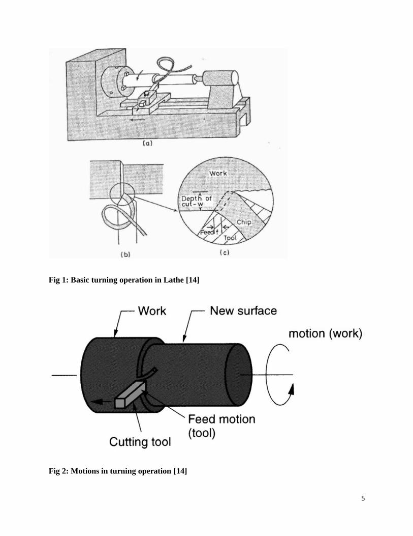
program. There are two types of motion in a turning operation. One is the cutting motion which

is the circular motion of the work and the other is the feed motion which is the linear motion

given to the tool. The basic turning operation with the motions involved is shown in Fig 1 and

Fig 2, figures from [14]. Fig 3 from [15] shows a single point cutting tool and its nomenclature.

5

Fig 1: Basic turning operation in Lathe [14]

Fig 2: Motions in turning operation [14]

6

Fig 3: Single point cutting tool using in turning and its nomenclature [15]

2.3. MACHINING PARAMETERS

The turning operation is governed by geometry factors and machining factors. This study

consists of the three primary adjustable machining parameters in a basic turning operation viz.

speed, feed and depth of cut. Fig 4 from [2] shows these three parameters. Material removal is

obtained by the combination of these three parameters [14]. Other input factors influencing the

output parameters such as surface roughness and tool wear also exist, but the latter are the ones

that can be easily modified by the operator during the course of the operation [15].

7

2.3.1 Cutting Speed

Cutting speed may be defined as the rate at which the uncut surface of the work piece

passes the cutting tool [1]. It is often referred to as surface speed and is ordinarily expressed in

m/min, though ft./min is also used as an acceptable unit [1,16]. Cutting speed can be obtained

from the spindle speed. The spindle speed is the speed at which the spindle, and hence, the work

piece, rotates. It is given in terms of number of revolutions of the work piece per minute i.e. rpm.

If the spindle speed is „N‟ rpm, the cutting speed V c (in m/min) is given as

V c =

---------------------- (1)

where, D = Diameter of the work piece in mm

2.3.2 Feed

Feed is the distance moved by the tool tip along its path of travel for every revolution of

the work piece. It is denoted as „f‟ and is expressed in mm/rev. Sometimes, it is also expressed in

terms of the spindle speed in mm/min as

F m = f N ---------------------- (2)

where, f = Feed in mm/rev

N = Spindle speed in rpm

8

2.3.2 Depth of cut

Depth of cut (d) is defined as the distance from the newly machined surface to the uncut

surface. In other words, it is the thickness of material being removed from the work piece. It can

also be defined as the depth of penetration of the tool into the work piece measured from the

work piece surface before rotation of the work piece. The diameter after machining is reduced by

twice of the depth of cut as this thickness is removed from both sides owing to the rotation of the

work.

d =

---------------------- (3)

where, D1 = Initial diameter of job

D2 = Final diameter of job

Fig 4: The adjustable machining parameters [2]

9

2.4 CUTTING TOOL

A cutting tool can be defined as a part of a machine tool that is responsible for removing the

excessive material from the work piece by direct mechanical abrasion and shear deformation

[13,17]. According to Choudhury et. al [16] and Schenider [18], an efficient cutting tool should

have the following characteristics –

a) Hardness: The tool material should be harder than the work material.

b) Hot hardness: The tool must maintain its hardness at elevated temperatures

encountered during the machining process.

c) Wear Resistance: The tool should have served to its acceptable level of life before it

wears out and needs to be replaced.

d) Toughness: The material should be strong enough so as to withstand shocks and

vibrations. During interrupted cutting, the tool should not chip or fracture.

For the ensuing study, the cutting tool used will be a clamped insert-type tool.

2.4.1 Cutting Tool Insert

The term „Insert‟ refers to the condition when a cutting tool is screwed or clamped to a

holder which is in turn fixed to the tool post. Inserts are clamped through various locking

mechanisms [19]. The advantage of inserts is that when one particular edge is worn out, it can be

rotated to present a new cutting edge. In certain cases, if the geometry allows, after all such

edges have been used up; the insert can be removed, turned upside down and clamped again to

10

reveal a fresh array of cutting edges. Inserts come in a varied range of shapes and sizes some of

which are shown in Fig 5 from [14].

Fig 5: Various shapes of cutting tool inserts [14]

2.4.1.1 Insert Material

There is a large variety of cutting tool materials that are available, each having its own

specific properties and performance abilities. Examples of insert materials are Carbides, HSS,

CBN, Diamond, Carbon speed steels etc. Carbide tools find common use in the metal cutting

industry due to their ability to machine at elevated temperatures and higher speeds [17].

11

2.4.1.2 Insert Coating

The cutting tool insert is coated to add improvement factors to it [19]. There is a variety

of coating materials each having their own specific applications and advantages. Physical vapour

deposition (PVD) method is one of the widely used methods used to achieve the coating of a

cutting tool. Another technique is Chemical vapour deposition (CVD). The CVD coating

technique requires higher temperature which makes it unfeasible for coating tool steels. Usage of

PVD method in order to apply Titanium Nitride (TiN) can be achieved at a much lower

temperatures (around 40000 C) [20]. PVD also facilitates the formation of sharper corners and

lower coefficient of friction [17].

2.5 TOOL WEAR

Tool wear is an inherent occurrence in every conventional machining process. Bin Halim said

that the tool wear is analogous to the gradual wear of the tip of a pencil [14]. It is the gradual

failure of cutting tools due to regular operation [17]. The tool wear rate is dependent on the tool

material itself, the tool shape and geometry, work piece material etc. The foremost important

factors affecting the tool wear which can be easily controlled are process parameters.

A key factor in the rate of tool wear of materials is the temperature achieved during machining.

The general idea is that energy expended in cutting is converted into heat and that a large

fraction of it is taken away in the chip. This results in about 20% of the heat generated going into

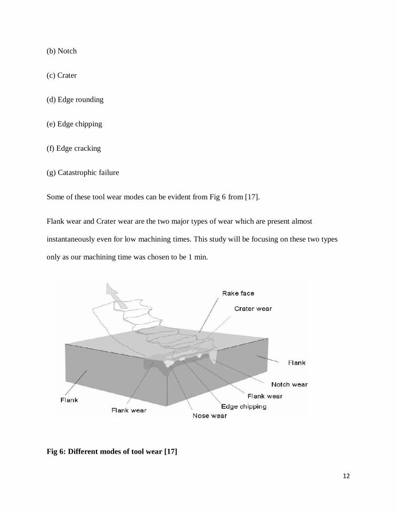
the cutting tool. The following types of tool wear modes can be observed [15]:

(a) Flank

12

(b) Notch

(c) Crater

(d) Edge rounding

(e) Edge chipping

(f) Edge cracking

(g) Catastrophic failure

Some of these tool wear modes can be evident from Fig 6 from [17].

Flank wear and Crater wear are the two major types of wear which are present almost

instantaneously even for low machining times. This study will be focusing on these two types

only as our machining time was chosen to be 1 min.

Fig 6: Different modes of tool wear [17]

13

2.5.1 Flank Wear

Flank wear (Fig 7, figure from [17]) is the wear that occurs on the flank surface or flank

faces of the cutting tool. This occurs due to direct mechanical abrasion and friction between the

flank surface and the work piece during the operation [21]. The width of the wear land is a

straightforward measure of the flank wear [14]. The width is denoted as VB. The tool life is

conventionally considered to be over when the average flank wear land VB reaches 300 µm or the

maximum flank wear land VB max becomes 600 µm [21]. Choudhury and Srinivas [22], found

that cutting speed and diffusion coefficient index have the most notable effect on the flank wear,

followed by feed and depth of cut.

Fig 7: Flank wear [17]

14

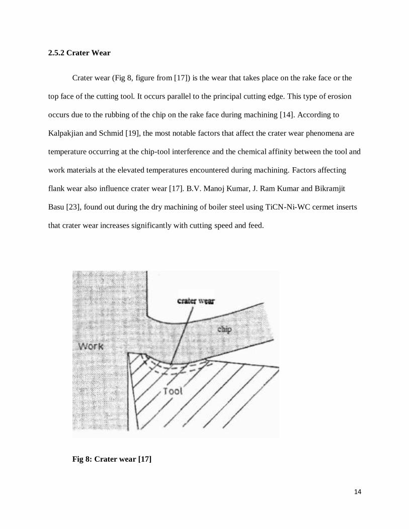
2.5.2 Crater Wear

Crater wear (Fig 8, figure from [17]) is the wear that takes place on the rake face or the

top face of the cutting tool. It occurs parallel to the principal cutting edge. This type of erosion

occurs due to the rubbing of the chip on the rake face during machining [14]. According to

Kalpakjian and Schmid [19], the most notable factors that affect the crater wear phenomena are

temperature occurring at the chip-tool interference and the chemical affinity between the tool and

work materials at the elevated temperatures encountered during machining. Factors affecting

flank wear also influence crater wear [17]. B.V. Manoj Kumar, J. Ram Kumar and Bikramjit

Basu [23], found out during the dry machining of boiler steel using TiCN-Ni-WC cermet inserts

that crater wear increases significantly with cutting speed and feed.

Fig 8: Crater wear [17]

15

2.6 SURFACE ROUGHNESS

Surface roughness is a measure of the surface finish of a product and an index of the product

quality [3]. Surface roughness is a measurement of the small scale variations in the height of a

physical surface [14]. It is expressed in various ways and methods, like arithmetic mean or

centre-line average (Ra), Root-mean square average (Rq), maximum peak (Ry), ten-point mean

roughness (Rz), maximum valley depth (Rv), maximum height of profile (Rt = Rp – Rv) etc. Out

of all these, the most commonly used indicator for surface roughness is Ra.

Ra, or the arithmetic mean value, previously known as AA (Arithmetic Average) or CLA

(Centre-Line Average) is the arithmetic mean of deviations of a series of points from the centre

line or datum line. The datum line is such that sum of the areas under the profile above the datum

will be equal to the sum of areas below the datum. Generally, surface roughness is expressed in

microns (μm).

Ra =

-------------- (4)

Fig 9: Co-ordinates used for Surface Roughness Measurement using Equation 4 [17]

16

Studies by Sahin Y. and Motorcu A.R., have shown that surface roughness is mostly dependent

on feed rate which is the dominating factor [24].

The surface roughness is usually measured in a direct way by the use of devices called

Profilometer. The Profilometer is a stylus probe instrument in which the stylus mounted in the

pick-up unit traverses across the machined surface by means of a motor drive. The pick-up

receives ad rectifies the output which is further amplified and the average height of the

roughness is reported digitally. One of the common types of Profilometer available is the Taylor-

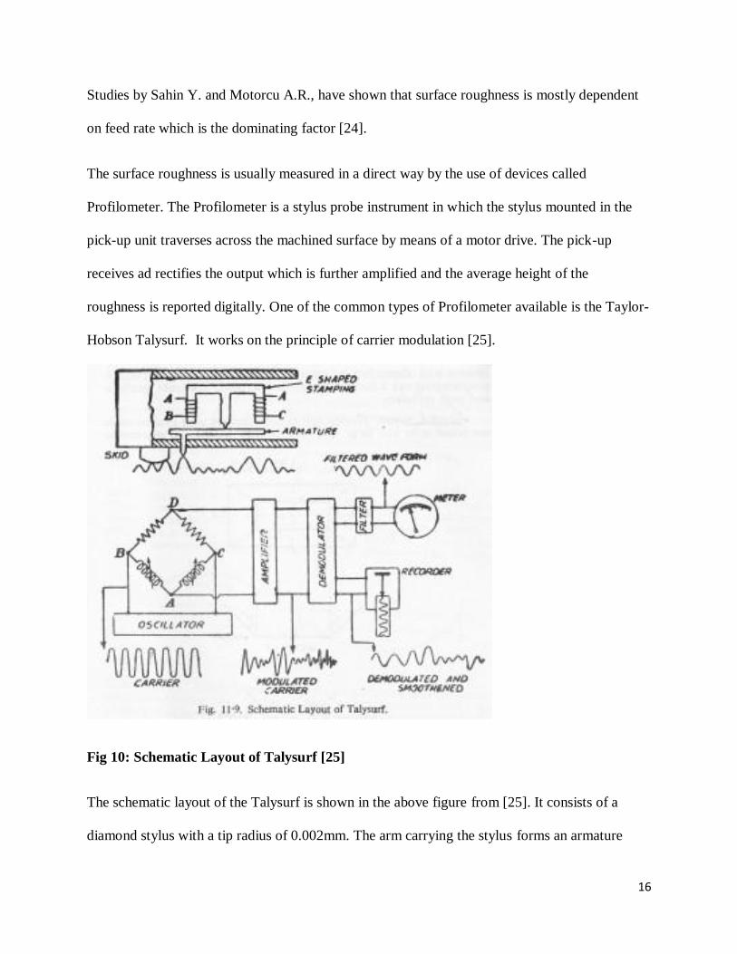
Hobson Talysurf. It works on the principle of carrier modulation [25].

Fig 10: Schematic Layout of Talysurf [25]

The schematic layout of the Talysurf is shown in the above figure from [25]. It consists of a

diamond stylus with a tip radius of 0.002mm. The arm carrying the stylus forms an armature

17

which pivots about the center leg of E-shaped stamping. Coils are wound around the two outer

legs of the E-shaped stamping and they carry alternating current. These two coils with other two

resistances form an oscillator. Movements in the stylus cause a variation in the air gap between

the armature and the stamping thereby modulating the amplitude of the alternating current. The

demodulator demodulates the signals such that the current becomes directly proportional to only

the vertical displacements of the stylus. The output is fed to a recorder which records and

produces the numerical output [25].

2.7 DESIGN OF EXPERIMENTS

Design of experiments (DOE) is a structured method that is used to identify relationships

between several input variables and output responses. With the help of DOE, the resources

needed to carry out the experiment can be optimized [14]. Hence, it finds wide use in R & D

studies. A few methods used as DOE are Taguchi Method, Response Surface Method and

Factorial Designs. We will be focusing on the Response Surface Methodology during the

ensuing study.

2.7.1 Response Surface Methodology (RSM)

Response Surface Method (RSM) is a collection of mathematical and statistical tools

which are useful for the modelling and analysis of problems in which an output response of

interest is influence by several input variables and our objective is to optimize (minimize or

maximize based on the need) the response [10]. It is a method which was developed by Box and

18

Wilson in the early 1950‟s [9]. It is capable of establishing causal relationships between input

and output variables.

For „n‟ number of measurable input variables, the response surface can be given as –

Y = f(x 1, x 2, x 3, x 4…x n ) + ε -----------(5)

Where, x 1 …x n are the independent input parameters and ε is the random error.

Y is the output or response variable which has to be optimized.

In a turning operation with three input variables, the response function can be written as –

Y = f(x 1, x 2, x 3) + ε ----------- (6)

Where, x 1 = log V c , x 2 = log f, and x 3 = log d. Y = log Ra and ε is the random error.

RSM is generally employed through multiple regression models. Our goal is to find a suitable

approximation for the response function which can be achieved by the regression models.

For example, the first order or linear multiple regression model can be used –

Y = β 0 +β1 x1 + β2 x2 + β3 x3 + ε ----------- (7)

For better approximation, interaction terms can be included –

Y = β 0 +β1 x1 + β2 x2 + β3 x3 + β12 x1 x2 + β13 x1 x3 + β23 x2 x3 + ε ----------- (8)

The second order or quadratic regression model includes the square terms in addition to the

terms above –

Y = β 0 +β1 x1 + β2 x2 + β3 x3 + β11 x12

+ β22x22

+ β33 x32

+ β12 x1 x2 + β13 x1 x3 + β23 x2 x3 + ε ---(9)

19

The quadratic model given in Equation 9 is generally utilized in RSM problems, the ease

being that there are some nice designs available for fitting quadratic models ex. Central

Composite Design (CCD) and Box-Behnken Design.

2.7.1.1 Central Composite Design (CCD)

CCD is one of the most popular designs for fitting the second-order models. Generally,

the CCD consists of a 2k factorial design with n j runs, 2k axial or star runs, and n c centre runs

[26]. The figure below (Fig 11) from [26] shows the CCD for k = 2 and k = 3 factors.

(a) k = 2 (b) k = 3

Fig 11: Central Composite Design for 2-factors and 3-factors [26]

First, a 2k first order model is used. If the model shows a lack of fit, then axial and center runs

are added to incorporate the quadratic terms in the model [26]. It is important to select the value

of α for the axial runs. If α = 1, the design is said to face-centered. The number of center points is

also to be selected. For a CCD with 3 input parameters, 6 centre points are generally chosen to

get 20 as the total number of runs including 8 cube points (cube corners and 6 axial/star points

(Fig b)

20

Chapter 3 MATERIALS AND METHODS

3.1 WORK MATERIAL

The work piece used for the concluded experiment was AISI 202 grade Austenitic stainless steel.

There are two series of Austenitic stainless steels – 300-series and 200-series. 300 series steels

find most wide use around the world but 200 series have become very popular in the Asian

subcontinent as an alternative to the 300 series to counter the increase in prices of Nickel [27].

Grade 202 steel can be made into plates, sheets and coils and finds extensive use in restaurant

equipment, cooking utensils, sinks, automotive trims, architectural applications such as doors

and windows, railways cars, trailers, horse clamps etc. [28]

Table 1: Chemical composition (wt %) of AISI 202 Steel

Element Wt %

Iron, Fe 68

Chromium, Cr 17-19

Nickel, Ni 4-6

Manganese, Mn 7.5-10

Silicon, Si 1

Nitrogen, N 0.25

Carbon 0.15

Phosphorous, P 0.06

Sulphur, S 0.03

21

Table 2: Mechanical Properties of AISI 202 Steel

Property Value

Tensile Strength 515 MPa

Yield Strength 275 Mpa

Elastic Modulus 207 Gpa

Poisson‟s Ratio 0.27-0.30

Elongation at break 40%

3.2 INSERT MATERIAL

The tool insert chosen was a coated carbide tool (Kennametal make) whose specifications are

shown below. Coated carbide tools are found to perform better than uncoated ones [11].

Table 3: Specification of Cutting Tool

ISO

Catalog

Number

ANSI

Catalog

Number

Grade Dimensions

D L10 S R ε D1

mm in mm in mm in mm in mm in

SNMG

120408

SNMG

432MS

KCU25 12.70 0.5 12.70 0.5 4.76 0.1875 5.16 0.203

The chosen insert (Fig 12 from [29]) was a square type negative insert meaning that it was

rotatable and reversible so that a total number of 8 cutting edges can be generated. KCU25 takes

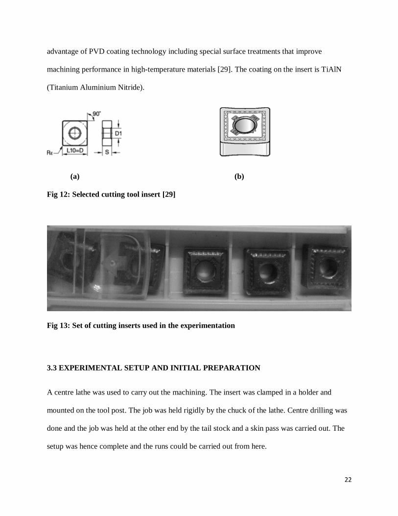
22

advantage of PVD coating technology including special surface treatments that improve

machining performance in high-temperature materials [29]. The coating on the insert is TiAlN

(Titanium Aluminium Nitride).

(a) (b)

Fig 12: Selected cutting tool insert [29]

Fig 13: Set of cutting inserts used in the experimentation

3.3 EXPERIMENTAL SETUP AND INITIAL PREPARATION

A centre lathe was used to carry out the machining. The insert was clamped in a holder and

mounted on the tool post. The job was held rigidly by the chuck of the lathe. Centre drilling was

done and the job was held at the other end by the tail stock and a skin pass was carried out. The

setup was hence complete and the runs could be carried out from here.

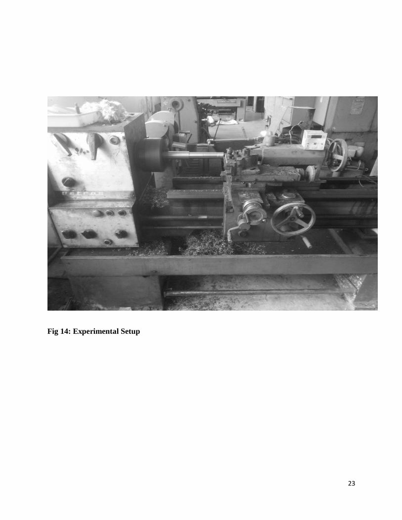
23

Fig 14: Experimental Setup

24

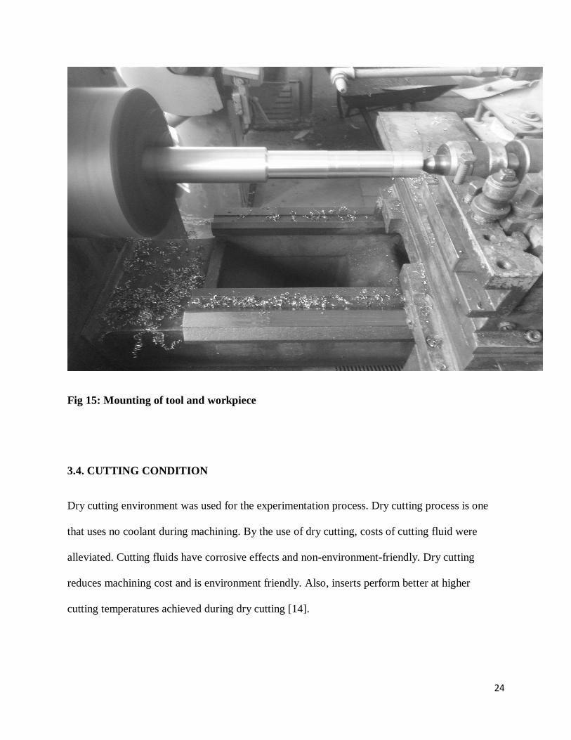
Fig 15: Mounting of tool and workpiece

3.4. CUTTING CONDITION

Dry cutting environment was used for the experimentation process. Dry cutting process is one

that uses no coolant during machining. By the use of dry cutting, costs of cutting fluid were

alleviated. Cutting fluids have corrosive effects and non-environment-friendly. Dry cutting

reduces machining cost and is environment friendly. Also, inserts perform better at higher

cutting temperatures achieved during dry cutting [14].

25

3.5 MEASUREMENT OF SURFACE ROUGHNESS

Surface roughness has been precisely measured with the help of a portable stylus-type

profilometer, Talysurf (Taylor Hobson, Surtronic 3+, UK). Measurements were taken at different

locations and the average was reported for each run.

Fig 16: Setup of Talysurf for measurement of Surface Roughness

Fig 17: Reading shown in Talysurf

26

3.6 MEASUREMENT OF TOOL WEAR

A new cutting edge was used for each run. The resulting tool wear was measured using a

Toolmaker‟s Microscope (Fig 18) with digital read-out device (Fig 20). A view of the tool insert

through the eyepiece is also shown in Fig 19.

Table 4: Specification of Toolmaker’s Microscope

1.1 Nr 14832

DDR Made in the CDR

Achsenhohe 42.52 mm 1554

Fig 18: Toolmakers’ Microscope

27

Fig 19: View of the insert through the eyepiece

Fig 20: Digitized reading of tool wear

28

3.7 PROCESS PARAMETERS

The following table (Table 5) shows the levels of the cutting parameters chosen.

Table 5: Factors and levels for the Response Surface Study

Code Parameter Level (-1) Level (+1)

A Cutting Speed (m/min) 66 112

B Feed (mm/rev) 0.05 0.15

C Depth of cut (mm) 0.4 0.8

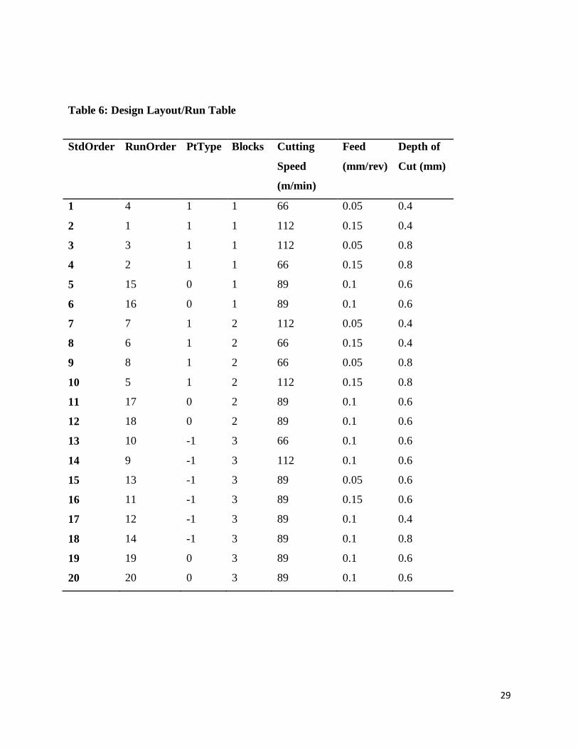
3.8 LAYOUT OF EXPERIMENT FOR RSM

The experiment layout was obtained in accordance with the 3-level full-factorial Central

Composite Design with 8 cube points, 6 axial points, 4 centre points, and 2 centre points in axial,

resulting in a total of 20 runs. α was chosen as 1 to make the design face centred. Table 6 below

contains the experimental layout used.

29

Table 6: Design Layout/Run Table

StdOrder RunOrder PtType Blocks Cutting

Speed

(m/min)

Feed

(mm/rev)

Depth of

Cut (mm)

1 4 1 1 66 0.05 0.4

2 1 1 1 112 0.15 0.4

3 3 1 1 112 0.05 0.8

4 2 1 1 66 0.15 0.8

5 15 0 1 89 0.1 0.6

6 16 0 1 89 0.1 0.6

7 7 1 2 112 0.05 0.4

8 6 1 2 66 0.15 0.4

9 8 1 2 66 0.05 0.8

10 5 1 2 112 0.15 0.8

11 17 0 2 89 0.1 0.6

12 18 0 2 89 0.1 0.6

13 10 -1 3 66 0.1 0.6

14 9 -1 3 112 0.1 0.6

15 13 -1 3 89 0.05 0.6

16 11 -1 3 89 0.15 0.6

17 12 -1 3 89 0.1 0.4

18 14 -1 3 89 0.1 0.8

19 19 0 3 89 0.1 0.6

20 20 0 3 89 0.1 0.6

30

Chapter 4 RESULTS AND DISCUSSIONS

4.1 EXPERIMENTAL RESULTS

The results obtained from the experimental work are summarized in the Table 7.

Table 7: Results Obtained

StdOrder RunOrder Cutting

Speed

(m/min)

Feed

(mm/rev)

Depth of

Cut (mm)

Ra

(µm)

Flank

wear

(mm)

1 4 66 0.05 0.4 0.947 0.443

2 1 112 0.15 0.4 1.513 0.768

3 3 112 0.05 0.8 1.353 0.932

4 2 66 0.15 0.8 1.7 1.17

5 15 89 0.1 0.6 0.86 1.629

6 16 89 0.1 0.6 0.887 1.209

7 7 112 0.05 0.4 0.88 0.487

8 6 66 0.15 0.4 1.947 0.57

9 8 66 0.05 0.8 1.893 1.104

10 5 112 0.15 0.8 1.673 1.151

11 17 89 0.1 0.6 1.053 1.844

12 18 89 0.1 0.6 1 1.604

13 10 66 0.1 0.6 1.16 0.928

14 9 112 0.1 0.6 0.96 1.001

15 13 89 0.05 0.6 2.16 0.948

16 11 89 0.15 0.6 2.013 0.859

17 12 89 0.1 0.4 1.413 0.788

18 14 89 0.1 0.8 1.007 1.116

19 19 89 0.1 0.6 0.967 1.807

20 20 89 0.1 0.6 0.96 1.793

31

4.2 ANALYSIS OF RESULTS AND PLOTS

The results obtained from the experiment were fed into MINITAB ® 17 for further analysis.

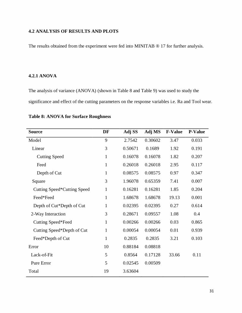
4.2.1 ANOVA

The analysis of variance (ANOVA) (shown in Table 8 and Table 9) was used to study the

significance and effect of the cutting parameters on the response variables i.e. Ra and Tool wear.

Table 8: ANOVA for Surface Roughness

Source DF Adj SS Adj MS F-Value P-Value

Model 9 2.7542 0.30602 3.47 0.033

Linear 3 0.50671 0.1689 1.92 0.191

Cutting Speed 1 0.16078 0.16078 1.82 0.207

Feed 1 0.26018 0.26018 2.95 0.117

Depth of Cut 1 0.08575 0.08575 0.97 0.347

Square 3 1.96078 0.65359 7.41 0.007

Cutting Speed*Cutting Speed 1 0.16281 0.16281 1.85 0.204

Feed*Feed 1 1.68678 1.68678 19.13 0.001

Depth of Cut*Depth of Cut 1 0.02395 0.02395 0.27 0.614

2-Way Interaction 3 0.28671 0.09557 1.08 0.4

Cutting Speed*Feed 1 0.00266 0.00266 0.03 0.865

Cutting Speed*Depth of Cut 1 0.00054 0.00054 0.01 0.939

Feed*Depth of Cut 1 0.2835 0.2835 3.21 0.103

Error 10 0.88184 0.08818

Lack-of-Fit 5 0.8564 0.17128 33.66 0.11

Pure Error 5 0.02545 0.00509

Total 19 3.63604

32

From Table 7, we can see that the P-Value for the model is 0.033 which is lesser than the

significance value of 0.05. Hence, the model is significant. The lack-of-fit has a P-value of 0.11

and hence, it is insignificant, which is desirable. Feed is found to be the most influential

parameter affecting the surface roughness with the lowest P-value among all three parameters.

Table 9: ANOVA for Tool Wear

Source DF Adj SS Adj MS F-Value P-

Value

Model 9 2.46551 0.273945 2.57 0.049

Linear 3 0.62221 0.207403 1.95 0.186

Cutting Speed 1 0.00154 0.001538 0.01 0.907

Feed 1 0.03648 0.036782 0.34 0.571

Depth of Cut 1 0.58419 0.584189 5.48 0.041

Square 3 1.80619 0.602063 5.65 0.016

Cutting Speed*Cutting

Speed 1 0.12033 0.120332 1.13 0.313

Feed*Feed 1 0.20075 0.200745 1.88 0.2

Depth of Cut*Depth of Cut 1 0.13514 0.135143 1.27 0.286

2-Way Interaction 3 0.03711 0.012369 0.12 0.949

Cutting Speed*Feed 1 0.01178 0.011781 0.11 0.746

Cutting Speed*Depth of

Cut 1 0.02344 0.023436 0.22 0.649

Feed*Depth of Cut 1 0.00189 0.001891 0.02 0.897

Error 10 1.06518 0.106518

Lack-of-Fit 5 0.8564 0.157088 2.81 0.141

Pure Error 5 0.27974 0.055948

Total 19 3.53068

From the above Table 8, we can see that the P-Value for the model is 0.049 which is lesser than

the significance value of 0.05. Hence, the model is significant. The lack-of-fit has a P-value of

0.141 and hence, it is insignificant, which is desirable. Depth of cut is found to be the most

influential parameter affecting the stool wear with the lowest P-value (0.041, significant) among

all three parameters.

33

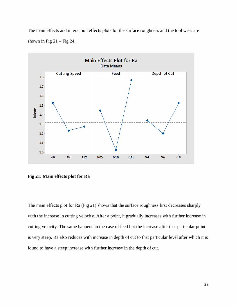
The main effects and interaction effects plots for the surface roughness and the tool wear are

shown in Fig 21 – Fig 24.

Fig 21: Main effects plot for Ra

The main effects plot for Ra (Fig 21) shows that the surface roughness first decreases sharply

with the increase in cutting velocity. After a point, it gradually increases with further increase in

cutting velocity. The same happens in the case of feed but the increase after that particular point

is very steep. Ra also reduces with increase in depth of cut to that particular level after which it is

found to have a steep increase with further increase in the depth of cut.

34

Fig 22: Interaction plot for Ra

Fig 23: Main effects plot for Tool wear

35

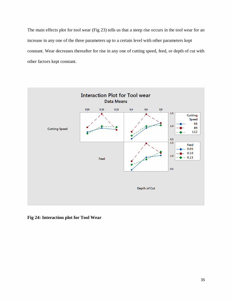
The main effects plot for tool wear (Fig 23) tells us that a steep rise occurs in the tool wear for an

increase in any one of the three parameters up to a certain level with other parameters kept

constant. Wear decreases thereafter for rise in any one of cutting speed, feed, or depth of cut with

other factors kept constant.

Fig 24: Interaction plot for Tool Wear

36

The regression coefficients obtained from MINITAB ® 17 are laid out in Tables 10 and 11.

Table 10: Estimated Coded Regression Coefficients for Surface Roughness

Term Effect Coef SE Coef T-Value P-Value

Constant 1.094 0.102 10.72 0

Cutting Speed -0.2536 -0.1268 0.0939 -1.35 0.207

Feed 0.3226 0.1613 0.0939 1.72 0.117

Depth of Cut 0.1852 0.0926 0.0939 0.99 0.347

Cutting Speed*Cutting Speed -0.487 -0.243 0.179 -1.36 0.204

Feed*Feed 1.566 0.783 0.179 4.37 0.001

Depth of Cut*Depth of Cut -0.187 -0.093 0.179 -0.52 0.614

Cutting Speed*Feed 0.037 0.018 0.105 0.17 0.865

Cutting Speed*Depth of Cut -0.017 -0.008 0.105 -0.08 0.939

Feed*Depth of Cut -0.376 -0.188 0.105 -1.79 0.103

Regression Equation in Un-coded Units:

Ra = -1.45 + 0.0758Vc – 49.5f + 5.30d – 0.00046Vc2 + 313.3f

2 – 2.33d

2 + 0.0519Vc*f –

0.0018Vc*d – 18.8f*d --------- (10)

37

Table 11: Estimated Coded Regression Coefficients for Tool Wear

Term Effect Coef SE Coef T-Value P-Value

Constant 1.458 0.112 13 0

Cutting Speed 0.025 0.012 0.103 0.12 0.907

Feed 0.121 0.06 0.103 0.59 0.571

Depth of Cut 0.483 0.242 0.103 2.34 0.041

Cutting Speed*Cutting Speed -0.418 -0.209 0.197 -1.06 0.313

Feed*Feed -0.54 -0.27 0.197 -1.37 0.2

Depth of Cut*Depth of Cut -0.443 -0.222 0.197 -1.13 0.286

Cutting Speed*Feed 0.077 0.038 0.115 0.33 0.746

Cutting Speed*Depth of Cut -0.108 -0.054 0.115 -0.47 0.649

Feed*Depth of Cut -0.031 -0.015 0.115 -0.13 0.897

Regression Equation in Un-coded Units:

Tool Wear = -6.07 + 0.0746Vc + 20.8f + 9.06 – 0.000395Vc2 – 108.1f

2 – 5.54d

2 + 0.033Vc*f -

0.0118Vc*d – 1.5f*d ------------ (11)

38

4.2.2 RESIDUAL PLOTS

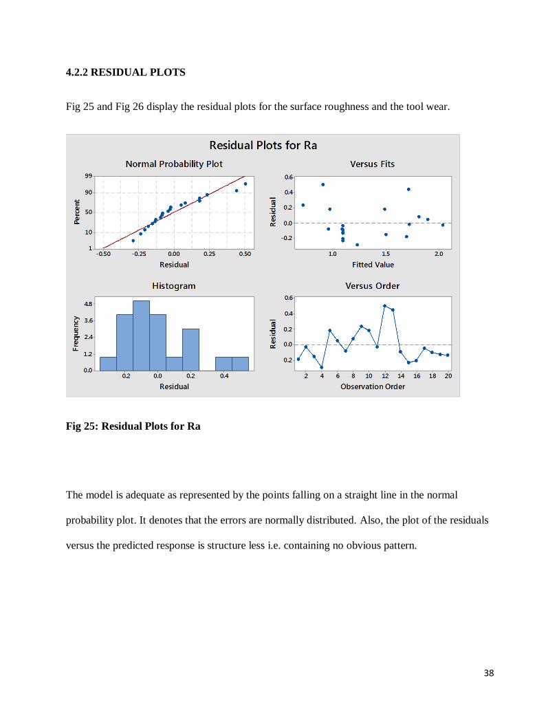
Fig 25 and Fig 26 display the residual plots for the surface roughness and the tool wear.

Fig 25: Residual Plots for Ra

The model is adequate as represented by the points falling on a straight line in the normal

probability plot. It denotes that the errors are normally distributed. Also, the plot of the residuals

versus the predicted response is structure less i.e. containing no obvious pattern.

39

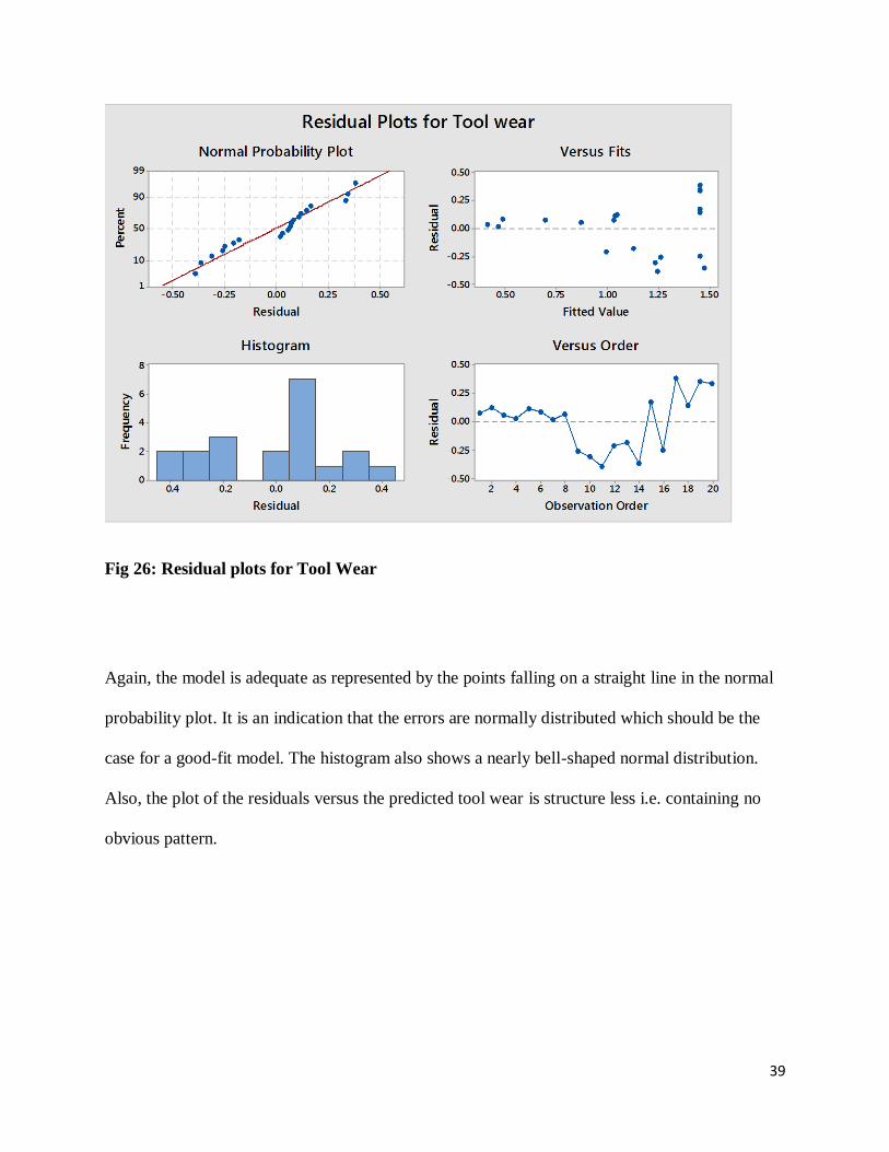
Fig 26: Residual plots for Tool Wear

Again, the model is adequate as represented by the points falling on a straight line in the normal

probability plot. It is an indication that the errors are normally distributed which should be the

case for a good-fit model. The histogram also shows a nearly bell-shaped normal distribution.

Also, the plot of the residuals versus the predicted tool wear is structure less i.e. containing no

obvious pattern.

40

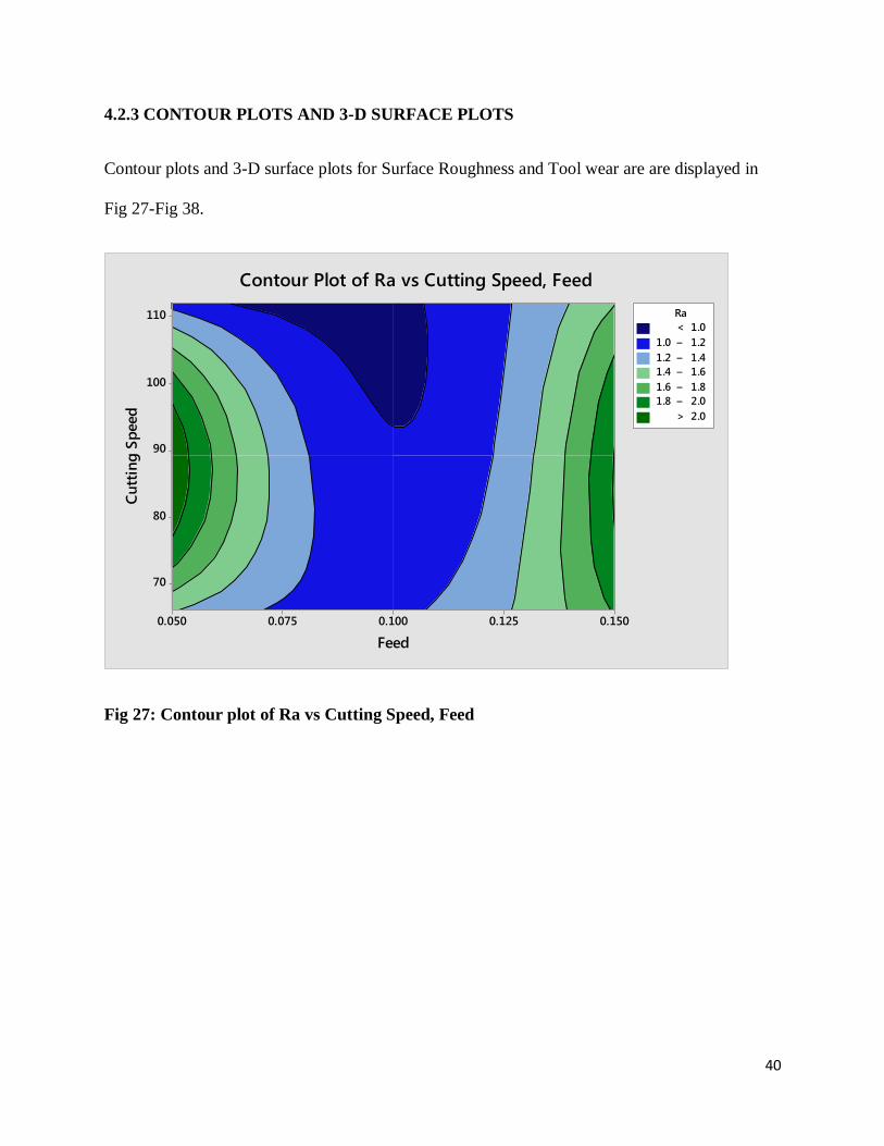
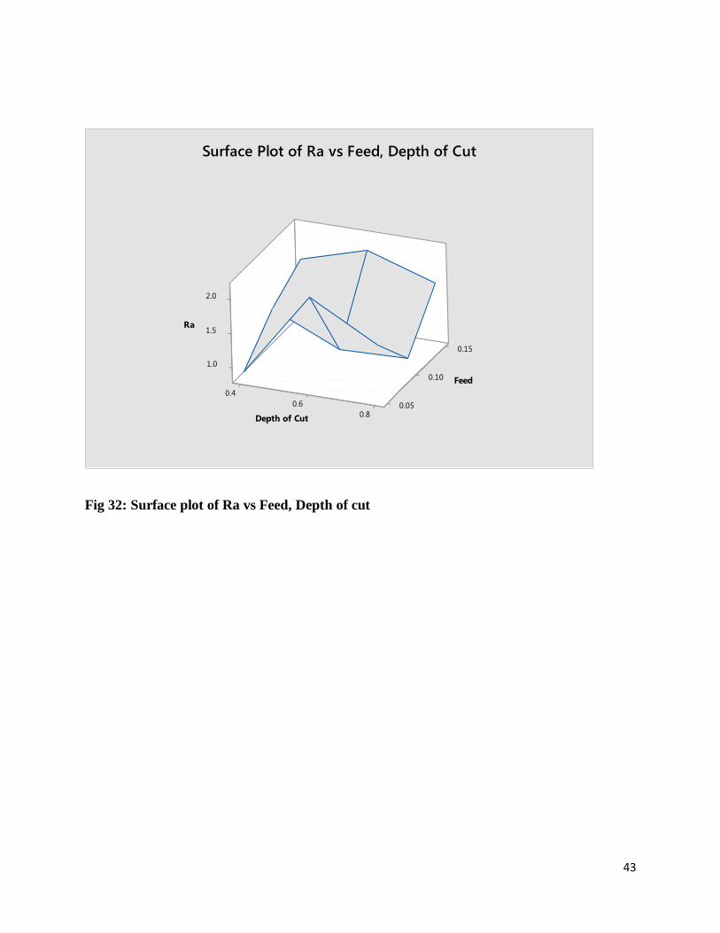
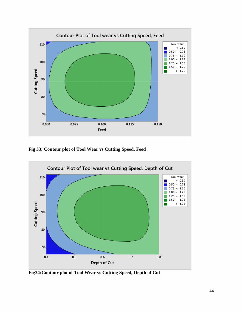
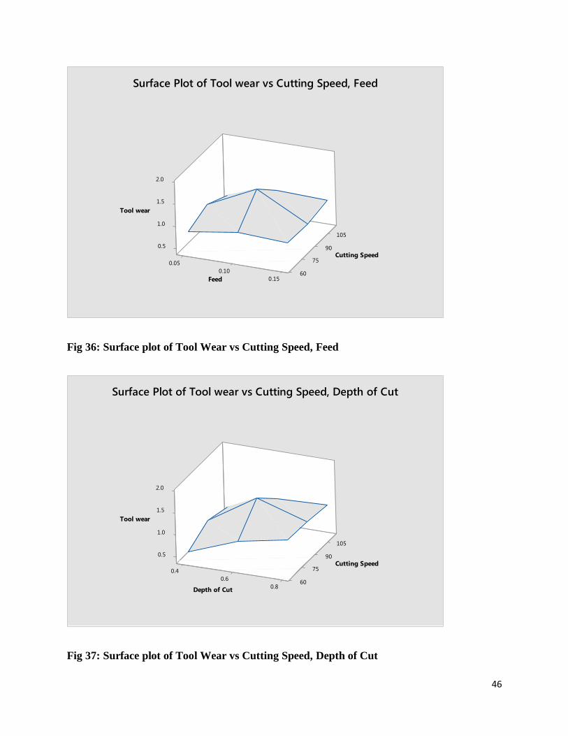
4.2.3 CONTOUR PLOTS AND 3-D SURFACE PLOTS

Contour plots and 3-D surface plots for Surface Roughness and Tool wear are are displayed in

Fig 27-Fig 38.

Fig 27: Contour plot of Ra vs Cutting Speed, Feed

Feed

Cu

ttin

g S

peed

0.1500.1250.1000.0750.050

110

100

90

80

70

>

–

–

–

–

–

< 1.0

1.0 1.2

1.2 1.4

1.4 1.6

1.6 1.8

1.8 2.0

2.0

Ra

Contour Plot of Ra vs Cutting Speed, Feed

41

Fig 28: Contour plot of Ra vs Cutting Speed, Depth of Cut

Fig29:Contour plot of Ra vs Feed, Depth of Cut

Depth of Cut

Cu

ttin

g S

peed

0.80.70.60.50.4

110

100

90

80

70

>

–

–

–

–

–

< 1.0

1.0 1.2

1.2 1.4

1.4 1.6

1.6 1.8

1.8 2.0

2.0

Ra

Contour Plot of Ra vs Cutting Speed, Depth of Cut

Depth of Cut

Feed

0.80.70.60.50.4

0.150

0.125

0.100

0.075

0.050

>

–

–

–

–

–

< 1.0

1.0 1.2

1.2 1.4

1.4 1.6

1.6 1.8

1.8 2.0

2.0

Ra

Contour Plot of Ra vs Feed, Depth of Cut

42

Fig 30: Surface plot of Ra vs Cutting Speed, Feed

Fig 31: Surface plot of Ra vs Cutting Speed, Depth of cut

501

90

0.1

1.5

0.05 57

2.0

1.0 0 0651.0

aR

deepS gnittuC

deeF

urface Plot of Ra vs Cutting SS eed, Feedp

501

09

0.1

1.5

0.4 75

2.0

0 6.60

8.0

aR

deepS gnittuC

tuC fo htpeD

urface Plot of Ra vs Cutting SpeS d, Depth of Cute

43

Fig 32: Surface plot of Ra vs Feed, Depth of cut

51.0

0.1

0.10

1.5

0 4.

2.0

6.0 0.058.0

aR

deeF

tuC fo htpeD

urface PlS t of Ra vo Feed, Depth of Cuts

44

Fig 33: Contour plot of Tool Wear vs Cutting Speed, Feed

Fig34:Contour plot of Tool Wear vs Cutting Speed, Depth of Cut

Feed

Cu

ttin

g S

peed

0.1500.1250.1000.0750.050

110

100

90

80

70

>

–

–

–

–

–

< 0.50

0.50 0.75

0.75 1.00

1.00 1.25

1.25 1.50

1.50 1.75

1.75

Tool wear

Contour Plot of Tool wear vs Cutting Speed, Feed

Depth of Cut

Cu

ttin

g S

peed

0.80.70.60.50.4

110

100

90

80

70

>

–

–

–

–

–

< 0.50

0.50 0.75

0.75 1.00

1.00 1.25

1.25 1.50

1.50 1.75

1.75

Tool wear

Contour Plot of Tool wear vs Cutting Speed, Depth of Cut

45

Fig 35: Contour plot of Tool Wear vs Feed, Depth of Cut

Depth of Cut

Feed

0.80.70.60.50.4

0.150

0.125

0.100

0.075

0.050

>

–

–

–

–

–

< 0.50

0.50 0.75

0.75 1.00

1.00 1.25

1.25 1.50

1.50 1.75

1.75

Tool wear

Contour Plot of Tool wear vs Feed, Depth of Cut

46

Fig 36: Surface plot of Tool Wear vs Cutting Speed, Feed

Fig 37: Surface plot of Tool Wear vs Cutting Speed, Depth of Cut

501

095.0

0.1

5.1

50.0 57

2.0

01.0 06.150

raew looT

deepS gnittuC

deeF

urface Plot of Tool S eaw vs Cutting Speed, Feedr

501

090.5

1.0

1.5

0 4. 75

2.0

6.060

8.0

l wearooT

gnituC t deepS

tuC feptD h o

urface Plot of TS ol wear vso Cutting Speed, Depth of Cut

47

Fig 38: Surface plot of Tool Wear vs Feed, Depth of Cut

51.0

5.001.0

0.1

1.5

.0 4

2.0

6.0 0.058.0

raew looT

deeF

tuC fo htpeD

urface Plot of Tool wear vs Feed, DepS h of Cutt

48

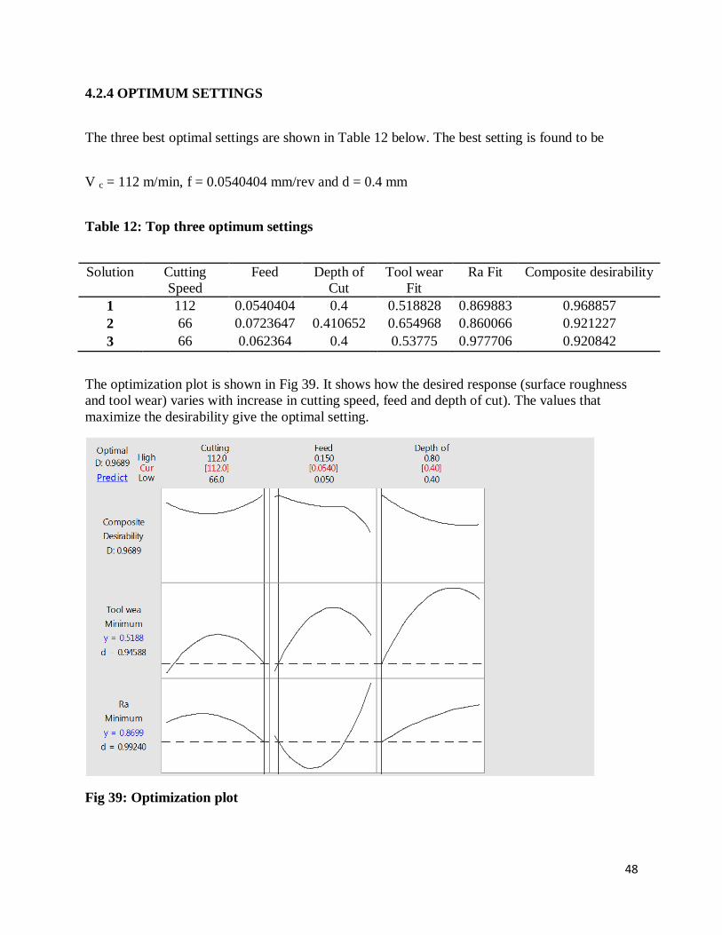
4.2.4 OPTIMUM SETTINGS

The three best optimal settings are shown in Table 12 below. The best setting is found to be

V c = 112 m/min, f = 0.0540404 mm/rev and d = 0.4 mm

Table 12: Top three optimum settings

Solution Cutting

Speed

Feed Depth of

Cut

Tool wear

Fit

Ra Fit Composite desirability

1 112 0.0540404 0.4 0.518828 0.869883 0.968857

2 66 0.0723647 0.410652 0.654968 0.860066 0.921227

3 66 0.062364 0.4 0.53775 0.977706 0.920842

The optimization plot is shown in Fig 39. It shows how the desired response (surface roughness

and tool wear) varies with increase in cutting speed, feed and depth of cut). The values that

maximize the desirability give the optimal setting.

Fig 39: Optimization plot

49

Chapter 6 CONCLUSIONS

6.1 CONCLUSIONS

RSM was successfully applied in optimizing the surface roughness and tool wear for the chosen

tool-work combination and for the selected domain of the input machining parameters. ANOVA

analysis was carried out and it is observed that feed is the most significant factor affecting the

surface roughness, closely followed by cutting speed and depth of cut, while the only significant

factor affecting the tool wear was found to be the depth of cut. The optimum running condition

was found to be at V c (112 m/min), f (0.0540404 mm/rev) and d (0.4 mm). Empirical models for

surface roughness and tool wear have been determined based on which predictions can be carried

out for output responses for appropriate applications.

6.2 SCOPE FOR FUTURE STUDY

The experiment was originally planned to be conducted with the involvement of mist application

of cutting fluid. Due to unavailability of the mist application device due to some constraints, the

experiment was conducted in a dry cutting environment. Mist application of cutting fluid could

be applied in the future to the same tool-work combination for the same domain of cutting

parameters as chosen in the present study and its effects on the surface roughness and tool wear

could be studied and analysed.

Another improvement that can be made to the present study is that cutting forces could be added

as an output response in addition to surface roughness and tool wear. An attempt can then be

50

made to find out optimum machining parameters so that multiple variables can be optimized via

a single experimental trial.

Furthermore, any tool geometry parameter from among nose its effects on the output responses

and in order to increase the effectiveness of the fitted model.

51

REFERENCES

1. Kumar, G., (2013), “Multi Objective Optimization of Cutting and Geometric parameters

in turning operation to Reduce Cutting forces and Surface Roughness,” B.Tech. thesis,

Department of Mechanical Engineering, National Institute of Technology, Rourkela.

2. Yang W.H. and Tarng Y.S., (1998), “Design optimization of cutting parameters for

turning operations based on Taguchi method,” Journal of Materials Processing

Technology, 84(1) pp.112–129.

3. Makadia A.J. and Nanavati J.I., (2013), “Optimisation of machining parameters for

turning operations based on response surface methodology,” Measurement, 46(4)

pp.1521-1529.

4. Neseli S., Yaldiz S. and Turkes E., (2011), “Optimization of tool geometry parameters

for turning operations based on the response surface methodology,” Measurement, 44(3),

pp. 80-587.

5. Bouacha K., Yallese M.A., Mabrouki T. and Rigal J.F., (2010), “Statistical analysis of

surface roughness and cutting forces using response surface methodology in hard turning

of AISI 52100 bearing steel with CBN tool,” International Journal of Refractory Metals

and Hard Materials, 28(3), pp. 349-361.

6. M.S. Lou, J.C. Chen and C.M. Li, (1999), “Surface roughness prediction technique for

CNC end-milling,” Journal of Industrial Technology, 15(1).

7. M.S. Lou and J.C. Chen, (1999), “In process surface roughness recognition system in

end-milling operations,” International Journal of Advanced Manufacturing Technology,

15(1) pp. 200–209.

52

8. Faisal, M.F.B.M., (2008), “Tool Wear Characterization of Carbide Cutting Tool

Inserts coated with Titanium Nitride (TiN) in a Single Point Turning Operation of AISI

D2 Steel,” B.Tech. thesis, Department of Manufacturing Engineering, Universiti

Teknikal Malaysia Mekala.

9. Sharma V.K., Murtaza Q. and Garg S.K., (2010), “Response Surface Methodology and

Taguchi Techniques to Optimization of C.N.C Turning Process,” International Journal of

Production Technology, 1(1), pp. 13-31.

10. Montgomery D.C., Design and Analysis of Experiments, 4th ed., Wiley, New York, 1997.

11. Noordin M.Y., Venkatesh V.C., Chan C.L. and Abdullah A., (2001), “Performance

evaluation of cemented carbide tools in turning AISI 1010 steel,” Journal of Materials

Processing Technology, 116(1) pp. 16–21.

12. Trent, E. and Wright, P. Metal Cutting, 4th ed., Butterworth-Heinemann, Woborn, MA,

Chap 2.

13. Dash, S.K., (2012), “Multi Objective Optimization of Cutting Parameters in Turning

Operation to Reduce Surface Roughness and Tool Vibration,” B.Tech. thesis, Department

of Mechanical Engineering, National Institute of Technology, Rourkela.

14. Halim, M.S.B., (2008), “Tool Wear Characterization of Carbide Cutting Tool

Insert in a Single Point Turning Operation of AISI D2 Steel,” B.Tech. thesis, Department

of Manufacturing Engineering, Universiti Teknikal Malaysia Mekala.

15. Khandey, U., (2009), “Optimization of Surface Roughness, Material Removal Rate and

cutting Tool Flank Wear in Turning Using Extended Taguchi Approach,” MTech thesis,

National Institute of Technology, Rourkela.

53

16. Hajra Chaudhury, S.K., Bose, S.K., Hajra Choudhury, A.K., Roy, N. and Bhattacharya

S.C. Elements of Workshop Technology Vol II: Machine Tools, 12th ed., Media Promoters

and Publishers, Mumbai, India, Chap 2.

17. Faisal, M.F.B.M., (2008), “Tool Wear Characterization of Carbide Cutting Tool

Inserts coated with Titanium Nitride (TiN) in a Single Point Turning Operation of AISI

D2 Steel,” B.Tech. thesis, Department of Manufacturing Engineering, Universiti

Teknikal Malaysia Mekala.

18. Schneider, S., (1989), “High speed machining: solutions for productivity,” Proceedings

of SCTE '89 Conference, San Diego, California.

19. Kalpakjian, S. and Schmid, S. Manufacturing Engineering and Technology, 7th

ed.,

Prentice Hall, New Jersey.

20. Ostwald, P.F. and Munoz, J. Manufacturing Processes and Systems, 9th ed., John Wiley

and Sons, New Delhi, India.

21. Gangopadhyay, S., 2013, Associate Professor at National Institute of Technology,

Rourkela, India, private communication.

22. Srinivas P. and Choudhury S.K., (2004), “Tool wear prediction in turning,” Journal of

Materials Processing Technology, 153(1) pp.276-280.

23. Manoj Kumar B.V., Ram Kumar J. and Basu B., (2007), “Crater wear mechanisms of

TiCN-Ni-WC cermets during dry machining,” International Journal of Refractory Metals

and Hard Materials, 25(5), pp. 392-399.

24. Sahin Y. and Motorcu A.R., (2008), “Surface roughness model in machining hardened

steel with cubic boron nitride cutting tool,” International Journal of Refractory Metals

and Hard Materials, 26(2), pp. 84-90 .

54

25. Mechlook, n.d, “Surface Finish – Direct Measurements,” from

http://www.mechlook.com/surface-finish-direct-instrument-measurements/

26. Ponnala W.D.S.M. and Murthy K.L.N., (2012), “Modelling and optimization of end

milling machining process,” International Journal of Research in Engineering and

Technology, 1(3), pp. 430-447.

27. M. Kaladhar, K. Venkata Subbaiah, Ch. Srinivasa Rao, and K. Narayana Rao, (2010),

“Optimization of Process Parameters in Turning of AISI202 austenitic stainless steel”,

ARPN Journal of Engineering and Applied Sciences, 5(9), pp. 79-87.

28. The A to Z of Materials, Azom, n.d., “Stainles Steel Grade 202 (UNS S20200),” from

http://www.azom.com/article.aspx?ArticleID=8209

29. Kennametal, n.d., “New Beyond Grades from Kennametal Add Productivity to Turning

Hard Alloys,” from http://www.kennametal.com/en/about-us/news/new-beyond-grades-

from-kennametal-add--productivity-to-turning-h.html