Optimization of LED illumination for generating metamerismDaisuke Miyazaki, Mia Nakamura, Masashi Baba, Ryo Furukawa, Shinsaku Hiura,Journal of Imaging Science and Technology,vol. 60, no. 6, pp. 60502-1-60502-15, 2016.11

http://www.cg.info.hiroshima-cu.ac.jp/~miyazaki/

This file is a draft version. It may be different from the published version.

Optimization of LED Illumination for Generating MetamerismDaisuke Miyazaki,1, a) Mia Nakamura,1, b) Masashi Baba,1 Ryo Furukawa,1 and Shinsaku Hiura1

Hiroshima City University, Graduate School of Information Sciences, 3-4-1 Ozukahigashi, Asaminami-ku, Hiroshima City,731-3194, Japan

Metamerism is the phenomenon by which two objects are recognized as having different colors under one light sourceand the same color under another light source. In this article, the authors propose a method for creating trick artworkusing metamerism. Two illuminants are designed to achieve metamerism such that two oil paints used in a piece ofartwork look the same under one light but different under another light. The experimental results show that metamerismis generated between the two light sources and the two object colors.

I. INTRODUCTION

The phenomenon by which two objects are recognizedas having different colors under one light source but as thesame color under another light source is called metamerism.Metamerism, which can cause the colors of clothing andprinted materials to vary under fluorescent lighting and sun-light, is known as a source of annoyance among designersand photographers, as well as those in the apparel, printing,and advertising industries. This article rebels against suchcommon sense and fully brings out the value of metamerism,which has been disregarded in the past. The proposed methodinvolves a multispectrum database of many types of light-emitting diode (LED). Two sets of light sources have beendesigned as mixtures of these LEDs so that two certain kindsof oil paint look identical under one but different under theother.

II. RELATED WORK

Computer-aided art software has made it possible for usersto create artwork that would have been very difficult to cre-ate manually1–8. This article proposes a new computer-aidedart system. Our system can be used to create metameric artsuch as that presented by Valluzzi9. Unlike Valluzzi9, whosepurpose was not to express intended figures, the objectiveof this paper is to design an illumination that can achievemetamerism so as to represent premeditated shapes.

Bala et al.10 also made watermarks using metamerism; be-cause CMYK printers can express black-colored prints eitherwith key (K) ink or cyan, magenta, and yellow (CMY) inks,they printed one of their black colors using K ink and anotherblack color using CMY ink. These colors appear the sameunder natural light but different when illuminated by LEDsof certain wavelengths. They selected an LED with a peakwavelength at which the spectral energies of two inks are suffi-ciently far apart to be distinguished visually. Drew and Bala11

improved their method to exaggerate the color difference10.Unlike Bala et al.10,11, we have designed an illumination thatcreates metamerism with user-suggested paints by combiningdifferent types of LEDs.

a)miyazaki@hiroshima-cu.ac.jpb)Presently with FUJITSU Kansai-Chubu Net-Tech, Ltd.

Finlayson et al.12,13 proposed a calculation method for aspectral distribution that achieves metamerism; their methodproduces various sets of spectral distributions that appear tohave the same color as a given RGB or XYZ value. Although,in theory, an infinite number of spectral distributions appear tobe the same color, Finlayson et al. confined the scope of theirarticle to those that could be expressed as linear sums of thespectral distributions of the Macbeth (X-rite) color checker. Inour article, we use LED spectral distributions as our databaseinstead of Macbeth color checker distributions, since we aimto design the illuminants using our LED database.

Miyazaki et al.14–16 proposed a method for calculating theblending ratios of paint that generate the metamerism in re-sponse to light sources suggested by the user. The paintshave wide-band spectral distributions, whereas the LEDs havenarrow-band spectral distributions, which can better repre-sent custom-built spectral distributions by using different LEDcombinations. Kobayashi et al.17 proposed a method for de-tecting cultivation colonies using images obtained by illumi-nating the medium with LEDs of different wavelengths. Un-like Miyazaki et al.14–16, who used paints for metameric art,Kobayashi17 and Bala10 have shown that LEDs are useful forenhancing color differences; their methods use only one LEDfor illuminating a single scene. This article proposes a methodthat calculates the LED-mixing ratios that generate the mostmetamerism possible given the oil paints used. We then cre-ate pieces of artwork that take advantage of the metamerismoccurring between the two suggested object colors under thetwo designed illuminant colors.

III. PERCEPTION OF REFLECTED LIGHT

The XYZ color system18,19 is a representative method forexpressing human perceptions of colors and was defined bythe Commission Internationale de l’Eclairage. It can expressthe colors perceived by the human brain stimulated by pho-toreceptor cells. The X, Y, and Z correspond to red, green,and blue, respectively. In general, the lower limit wavelengthof visible light is approximately 380–420 nm, and the upperlimit is approximately 680–800 nm20–23. In this article, weconsider light with wavelengths varying from 400 to 800 nmbecause our measurement device can only measure spectraldistributions within this range. Expressing the color-matchingfunctions of X, Y, and Z for a wavelength λ as x(λ), y(λ),and z(λ), respectively, the observed X, Y, and Z values are

2

Light ObjectSpectral responseCIE-XYZ value

LP bx

a.k.a.a.k.a.

diag(Ew)

XYZ

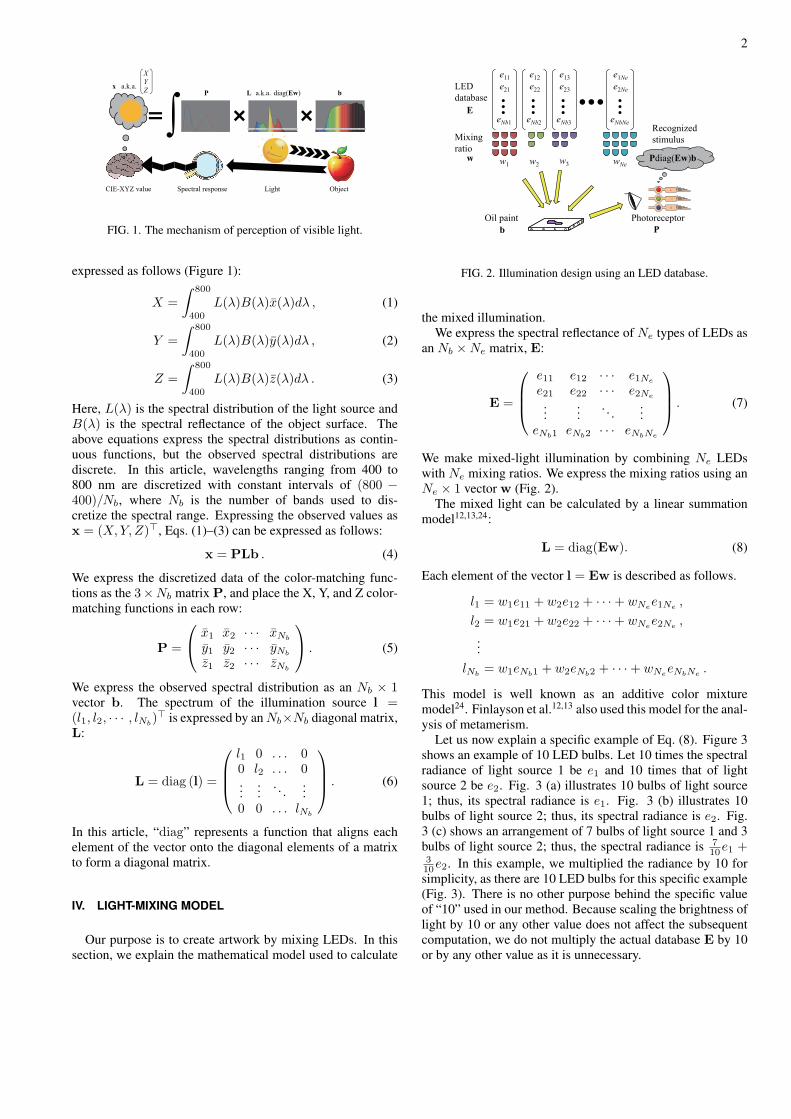
FIG. 1. The mechanism of perception of visible light.

expressed as follows (Figure 1):

X =

∫ 800

400

L(λ)B(λ)x(λ)dλ , (1)

Y =

∫ 800

400

L(λ)B(λ)y(λ)dλ , (2)

Z =

∫ 800

400

L(λ)B(λ)z(λ)dλ . (3)

Here, L(λ) is the spectral distribution of the light source andB(λ) is the spectral reflectance of the object surface. Theabove equations express the spectral distributions as contin-uous functions, but the observed spectral distributions arediscrete. In this article, wavelengths ranging from 400 to800 nm are discretized with constant intervals of (800 −400)/Nb, where Nb is the number of bands used to dis-cretize the spectral range. Expressing the observed values asx = (X,Y, Z)�, Eqs. (1)–(3) can be expressed as follows:

x = PLb . (4)

We express the discretized data of the color-matching func-tions as the 3×Nb matrix P, and place the X, Y, and Z color-matching functions in each row:

P =

⎛⎝ x1 x2 · · · xNb

y1 y2 · · · yNb

z1 z2 · · · zNb

⎞⎠ . (5)

We express the observed spectral distribution as an Nb × 1vector b. The spectrum of the illumination source l =(l1, l2, · · · , lNb

)� is expressed by an Nb×Nb diagonal matrix,L:

L = diag (l) =

⎛⎜⎜⎝

l1 0 . . . 00 l2 . . . 0...

.... . .

...0 0 . . . lNb

⎞⎟⎟⎠ . (6)

In this article, “diag” represents a function that aligns eachelement of the vector onto the diagonal elements of a matrixto form a diagonal matrix.

IV. LIGHT-MIXING MODEL

Our purpose is to create artwork by mixing LEDs. In thissection, we explain the mathematical model used to calculate

Oil paint Photoreceptor

LEDdatabase

Mixingratio

b P

w1 w2 w3 wNe

e11e21

eNb1

w

E

e12e22

eNb2

e13e23

eNb3 eNbNe

e1Nee2Ne

L

M

S

Recognizedstimulus

Pdiag(Ew)b

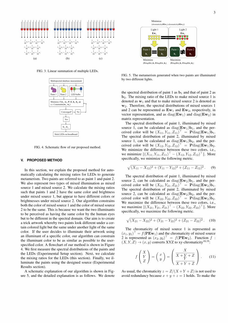
FIG. 2. Illumination design using an LED database.

the mixed illumination.We express the spectral reflectance of Ne types of LEDs as

an Nb ×Ne matrix, E:

E =

⎛⎜⎜⎝

e11 e12 · · · e1Ne

e21 e22 · · · e2Ne

......

. . ....

eNb1 eNb2 · · · eNbNe

⎞⎟⎟⎠ . (7)

We make mixed-light illumination by combining Ne LEDswith Ne mixing ratios. We express the mixing ratios using anNe × 1 vector w (Fig. 2).

The mixed light can be calculated by a linear summationmodel12,13,24:

L = diag(Ew). (8)

Each element of the vector l = Ew is described as follows.

l1 = w1e11 + w2e12 + · · ·+ wNee1Ne

,

l2 = w1e21 + w2e22 + · · ·+ wNee2Ne

,

...lNb

= w1eNb1 + w2eNb2 + · · ·+ wNeeNbNe

.

This model is well known as an additive color mixturemodel24. Finlayson et al.12,13 also used this model for the anal-ysis of metamerism.

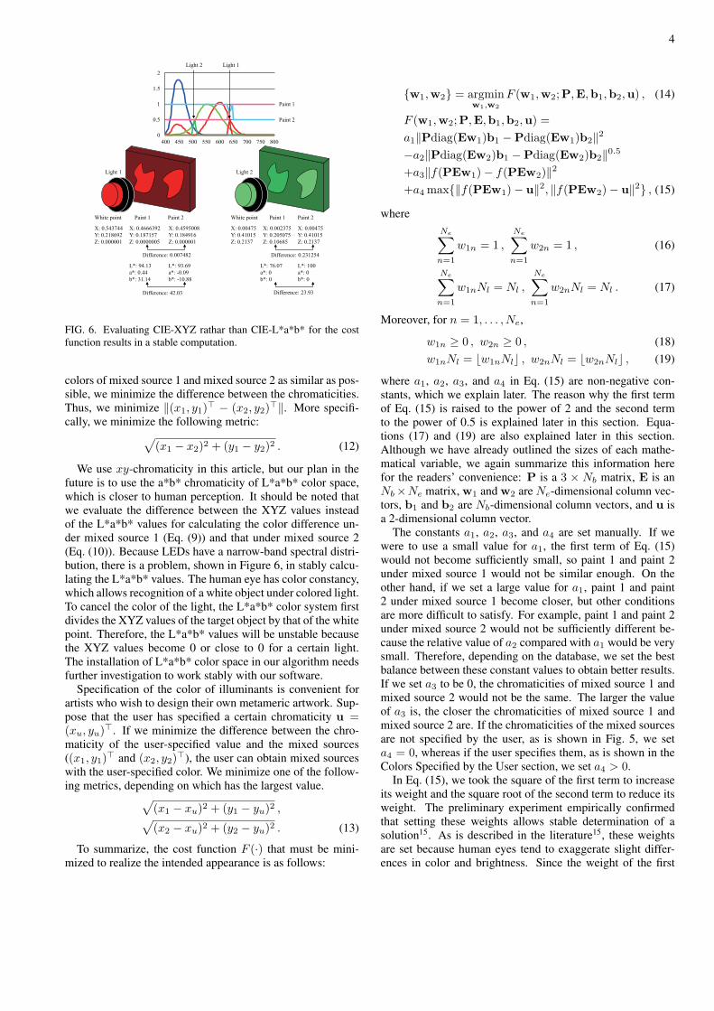
Let us now explain a specific example of Eq. (8). Figure 3shows an example of 10 LED bulbs. Let 10 times the spectralradiance of light source 1 be e1 and 10 times that of lightsource 2 be e2. Fig. 3 (a) illustrates 10 bulbs of light source1; thus, its spectral radiance is e1. Fig. 3 (b) illustrates 10bulbs of light source 2; thus, its spectral radiance is e2. Fig.3 (c) shows an arrangement of 7 bulbs of light source 1 and 3bulbs of light source 2; thus, the spectral radiance is 7

10e1 +310e2. In this example, we multiplied the radiance by 10 forsimplicity, as there are 10 LED bulbs for this specific example(Fig. 3). There is no other purpose behind the specific valueof “10” used in our method. Because scaling the brightness oflight by 10 or any other value does not affect the subsequentcomputation, we do not multiply the actual database E by 10or by any other value as it is unnecessary.

3

(a) (b) (c)

111

111

1111

101

101

101

101

101

101

101

101

101

101

eee

eee

eeee

222

222

2222

101

101

101

101

101

101

101

101

101

101

eee

eee

eeee

121

121

1211

101

101

101

101

101

101

101

101

101

101

eee

eee

eeee

FIG. 3. Linear summation of multiple LEDs.

Paint 1 Paint 2 LED bulbs

Minimize F(w1, w2; P, E, b1, b2, u)s.t. Constraints(w1, w2)

Converged?

Yes

No

w1, w2

Stick LEDs on breadboard

Multispectral database measurement

FIG. 4. Schematic flow of our proposed method.

V. PROPOSED METHOD

In this section, we explain the proposed method for auto-matically calculating the mixing ratios for LEDs to generatemetamerism. Two paints are referred to as paint 1 and paint 2.We also represent two types of mixed illumination as mixedsource 1 and mixed source 2. We calculate the mixing ratiossuch that paints 1 and 2 have the same color and brightnessunder mixed source 1, but appear to have different colors orbrightnesses under mixed source 2. Our algorithm constrainsboth the color of mixed source 1 and the color of mixed source2 to be the same. This is because we want the two illuminantsto be perceived as having the same color by the human eyesbut to be different in the spectral domain. Our aim is to createa trick artwork whereby two paints look different under a cer-tain colored light but the same under another light of the samecolor. If the user decides to illuminate their artwork usingan illuminant of a specific color, our algorithm can constrainthe illuminant color to be as similar as possible to the user-specified color. A flowchart of our method is shown in Figure4. We first measure the spectral distributions of the paints andthe LEDs (Experimental Setup section). Next, we calculatethe mixing ratios for the LEDs (this section). Finally, we il-luminate the paints using the designed source (ExperimentalResults section).

A schematic explanation of our algorithm is shown in Fig-ure 5, and the detailed explanation is as follows. We denote

Light 1 Light 2

Paint 1 Paint 2 Paint 1 Paint 2b1 b2 b1 b2

Ew1 Ew2

Minimize

Minimize Maximize

||chromaticity(PEw1)-chromaticity(PEw2)||

||Pdiag(Ew1)b1-Pdiag(Ew1)b2|| ||Pdiag(Ew2)b1-Pdiag(Ew2)b2||

FIG. 5. The metamerism generated when two paints are illuminatedby two different lights.

the spectral distribution of paint 1 as b1 and that of paint 2 asb2. The mixing ratio of the LEDs to make mixed source 1 isdenoted as w1 and that to make mixed source 2 is denoted asw2. Therefore, the spectral distributions of mixed sources 1and 2 can be represented as Ew1 and Ew2, respectively, invector representation, and as diag(Ew1) and diag(Ew2) inmatrix representation.

The spectral distribution of paint 1, illuminated by mixedsource 1, can be calculated as diag(Ew1)b1, and the per-ceived color will be (X11, Y11, Z11)

� = Pdiag(Ew1)b1.The spectral distribution of paint 2, illuminated by mixedsource 1, can be calculated as diag(Ew1)b2, and the per-ceived color will be (X12, Y12, Z12)

� = Pdiag(Ew1)b2.We minimize the difference between these two colors, i.e.,we minimize ‖(X11, Y11, Z11)

� − (X12, Y12, Z12)�‖. More

specifically, we minimize the following metric.√(X11 −X12)2 + (Y11 − Y12)2 + (Z11 − Z12)2 . (9)

The spectral distribution of paint 1, illuminated by mixedsource 2, can be calculated as diag(Ew2)b1, and the per-ceived color will be (X21, Y21, Z21)

� = Pdiag(Ew2)b1.The spectral distribution of paint 2, illuminated by mixedsource 2, can be calculated as diag(Ew2)b2, and the per-ceived color will be (X22, Y22, Z22)

� = Pdiag(Ew2)b2.We maximize the difference between these two colors, i.e.,we maximize ‖(X21, Y21, Z21)

� − (X22, Y22, Z22)�‖. More

specifically, we maximize the following metric.√(X21 −X22)2 + (Y21 − Y22)2 + (Z21 − Z22)2 . (10)

The chromaticity of mixed source 1 is represented as(x1, y1)

� = f(PEw1) and the chromaticity of mixed source2 is represented as (x2, y2)

� = f(PEw2). Function f :(X,Y, Z) → (x, y) converts XYZ to xy-chromaticity18,19:

f

⎛⎝ X

YZ

⎞⎠ =

(xy

)=

⎛⎜⎝

X

X + Y + ZY

X + Y + Z

⎞⎟⎠ . (11)

As usual, the chromaticity z = Z/(X+Y +Z) is not used toavoid redundancy because x+ y + z = 1 holds. To make the

4

0

0.5

1

1.5

2

400 450 500 550 600 650 700 750 800

Light 1 Light 2

White point White pointPaint 1 Paint 2 Paint 1 Paint 2

Paint 1

Paint 2

Light 1Light 2

X: 0.543744Y: 0.218692Z: 0.000001

X: 0.4666392Y: 0.187157Z: 0.0000005

X: 0.4595008Y: 0.184916Z: 0.000001

Difference: 0.007482

L*: 94.13a*: 0.44b*: 31.14

L*: 93.69a*: -0.09b*: -10.88

Difference: 42.03

X: 0.00475Y: 0.41015Z: 0.2137

X: 0.002375Y: 0.205075Z: 0.10685

X: 0.00475Y: 0.41015Z: 0.2137

Difference: 0.231254

L*: 76.07a*: 0b*: 0

L*: 100a*: 0b*: 0

Difference: 23.93

FIG. 6. Evaluating CIE-XYZ rathar than CIE-L*a*b* for the costfunction results in a stable computation.

colors of mixed source 1 and mixed source 2 as similar as pos-sible, we minimize the difference between the chromaticities.Thus, we minimize ‖(x1, y1)

� − (x2, y2)�‖. More specifi-

cally, we minimize the following metric:√(x1 − x2)2 + (y1 − y2)2 . (12)

We use xy-chromaticity in this article, but our plan in thefuture is to use the a*b* chromaticity of L*a*b* color space,which is closer to human perception. It should be noted thatwe evaluate the difference between the XYZ values insteadof the L*a*b* values for calculating the color difference un-der mixed source 1 (Eq. (9)) and that under mixed source 2(Eq. (10)). Because LEDs have a narrow-band spectral distri-bution, there is a problem, shown in Figure 6, in stably calcu-lating the L*a*b* values. The human eye has color constancy,which allows recognition of a white object under colored light.To cancel the color of the light, the L*a*b* color system firstdivides the XYZ values of the target object by that of the whitepoint. Therefore, the L*a*b* values will be unstable becausethe XYZ values become 0 or close to 0 for a certain light.The installation of L*a*b* color space in our algorithm needsfurther investigation to work stably with our software.

Specification of the color of illuminants is convenient forartists who wish to design their own metameric artwork. Sup-pose that the user has specified a certain chromaticity u =(xu, yu)

�. If we minimize the difference between the chro-maticity of the user-specified value and the mixed sources((x1, y1)

� and (x2, y2)�), the user can obtain mixed sources

with the user-specified color. We minimize one of the follow-ing metrics, depending on which has the largest value.√

(x1 − xu)2 + (y1 − yu)2 ,√(x2 − xu)2 + (y2 − yu)2 . (13)

To summarize, the cost function F (·) that must be mini-mized to realize the intended appearance is as follows:

{w1,w2} = argminw1,w2

F (w1,w2;P,E,b1,b2,u) , (14)

F (w1,w2;P,E,b1,b2,u) =

a1‖Pdiag(Ew1)b1 −Pdiag(Ew1)b2‖2−a2‖Pdiag(Ew2)b1 −Pdiag(Ew2)b2‖0.5+a3‖f(PEw1)− f(PEw2)‖2+a4 max{‖f(PEw1)− u‖2, ‖f(PEw2)− u‖2} , (15)

whereNe∑n=1

w1n = 1 ,

Ne∑n=1

w2n = 1 , (16)

Ne∑n=1

w1nNl = Nl ,

Ne∑n=1

w2nNl = Nl . (17)

Moreover, for n = 1, . . . , Ne,

w1n ≥ 0 , w2n ≥ 0 , (18)w1nNl = �w1nNl� , w2nNl = �w2nNl� , (19)

where a1, a2, a3, and a4 in Eq. (15) are non-negative con-stants, which we explain later. The reason why the first termof Eq. (15) is raised to the power of 2 and the second termto the power of 0.5 is explained later in this section. Equa-tions (17) and (19) are also explained later in this section.Although we have already outlined the sizes of each mathe-matical variable, we again summarize this information herefor the readers’ convenience: P is a 3 × Nb matrix, E is anNb×Ne matrix, w1 and w2 are Ne-dimensional column vec-tors, b1 and b2 are Nb-dimensional column vectors, and u isa 2-dimensional column vector.

The constants a1, a2, a3, and a4 are set manually. If wewere to use a small value for a1, the first term of Eq. (15)would not become sufficiently small, so paint 1 and paint 2under mixed source 1 would not be similar enough. On theother hand, if we set a large value for a1, paint 1 and paint2 under mixed source 1 become closer, but other conditionsare more difficult to satisfy. For example, paint 1 and paint 2under mixed source 2 would not be sufficiently different be-cause the relative value of a2 compared with a1 would be verysmall. Therefore, depending on the database, we set the bestbalance between these constant values to obtain better results.If we set a3 to be 0, the chromaticities of mixed source 1 andmixed source 2 would not be the same. The larger the valueof a3 is, the closer the chromaticities of mixed source 1 andmixed source 2 are. If the chromaticities of the mixed sourcesare not specified by the user, as is shown in Fig. 5, we seta4 = 0, whereas if the user specifies them, as is shown in theColors Specified by the User section, we set a4 > 0.

In Eq. (15), we took the square of the first term to increaseits weight and the square root of the second term to reduce itsweight. The preliminary experiment empirically confirmedthat setting these weights allows stable determination of asolution15. As is described in the literature15, these weightsare set because human eyes tend to exaggerate slight differ-ences in color and brightness. Since the weight of the first

5

term is larger than that of the second term, our software triesto minimize the first term much more than the second term.Thus, the slight color difference represented by the first termis suppressed. Finding spectral distributions that become thesame color is difficult. On the other hand, an infinite varietyof spectral distributions that can express different colors exist.Thus, this is another reason for setting such weights.

Because Eq. (14) is a complicated function with multipleconstraints, we employ a simulated annealing method25 basedon the Nelder–Mead downhill simplex method25 to solve itstably. The first and second terms of Eq. (15) consider notonly the chromaticity but also the brightness because the re-sultant illuminants must satisfy the requirement of enablingartistic illusion. When observing a scene illuminated only bymixed source 1 and another scene illuminated only by mixedsource 2, human pupils and photoreceptors automatically ad-just for the brightness; thus, the difference in brightness be-tween mixed source 1 and mixed source 2 does not affect ourmethod. However, the brightness calculated for mixed source1 and that for mixed source 2 must be simultaneously evalu-ated using Eq. (15). Thus, the sum of the elements of Ew1

is set to 1. Further, the sum of the elements of Ew2 is set to1. Any normalization procedures can be employed since thenormalization does not affect human perception because ofits ability to automatically adjust to incoming light. Equation(15) can be stably solved by adequately adjusting the coeffi-cients a1 and a2, regardless of the normalization procedureused.

The Nelder–Mead downhill simplex method25 expressesthe parameters to be solved as a simplex with 2Ne +1 apexesrepresented in a 2Ne-dimensional solution space. This sim-plex moves like an amoeba in the solution space toward thefinal solution where the value of the cost function is small.

The parameters w1 and w2 are normalized when evaluatingthe cost function, as shown in Eqs. (16)–(19); however, theseparameters are not normalized when updating the simplex, sothat the simplex can freely deform in the solution space.

We use random values for the initial state of the simplex.The original Nelder–Mead downhill simplex method25 usesthe unit vectors lying on each axis of the solution space asinitial values. Namely, the initial value of the nth apex an isexpressed as follows, except in the case of a2Ne+1, which isset to be a zero vector:

ank =

{1 (if n = k) ,0 (if n �= k) .

(20)

However, we cannot set the same initial value as in the orig-inal simplex method because the parameters in our situationshould satisfy the conditions shown in Eqs. (16) and (18).Therefore, the initial value for n = 1, . . . , 2Ne should be setas follows:

an =an

2Ne∑k=1

ank

(21)

ank =

{100 (if n = k)1 (if n �= k) .

-1.6-1.5-1.4-1.3-1.2-1.1

-1-0.9-0.8-0.7-0.6-0.5-0.4-0.3-0.2

Number of trials

Final cost valueif our initial value is used

Final cost valueif original initialvalue is used

FIG. 7. The final cost value when the random initial values are used.

The (2Ne + 1)th apex is set as follows:

a2Ne+1,k =1

Ne. (22)

The value of the cost function shown in Eq. (15) was 44.137for these initial parameters, with certain coefficients set fora1, a2, a3, and a4. After optimization using Eq. (14), the costvalue was decreased to −1.079.

Next, we set random values for the initial state of the sim-plex. We have tried 100 sets of initial values with optimiza-tion. The cost value for each set is shown as the vertical barsin Fig. 7. The horizontal line shows the cost value −1.079.The worst value (the largest value) was −0.319 and the bestvalue (the smallest value) was −1.525 for these 100 experi-mental results. The average was −1.046 and the standard de-viation was 0.173. Out of 100 trials, 36 sets produced betterresults than when the initial values were set as in Eqs. (21) and(22). Because we can obtain better results if we set the randomseed adequately, it is better to use random values for the initialstates. On the other hand, compared with the initial cost value44.137, the range of the final cost value, which varies from−0.319 to −1.525, is narrow. Therefore, we can state thatthe optimization method25 stably produces sufficiently goodresults for a variety of initial values. We therefore did not tryto find another way to set the initial values, and we concludedthat setting random values for the initial state is sufficient forour purposes.

Here, we explain Eqs. (17) and (19). Mixed-light sourcesare created by placing certain LED bulbs on a solderlessbreadboard, with the bulbs being selected based on the mix-ing ratios calculated in the preceding sections. We representthe number of LED bulbs stuck on a solderless breadboard asNl. Since the sum of the mixing ratio is 1, we constrain themixing ratio wn to be an integer multiple of 1/Nl. The detailsof this procedure are given in Algorithm 1.

Fig. 8 shows a specific example of 10 LEDs (Nl = 10) se-lected from 15 different types (Ne = 15) stuck on a solderlessbreadboard.

The cost function (Eq. (15)) becomes a non-smooth discretefunction because of the discrete representation of the mixingratio wn. The steepest descent method, conjugate gradientmethod, and Levenberg–Marquardt method are inappropriatefor this reason. Instead, the Nelder–Mead downhill simplex

6

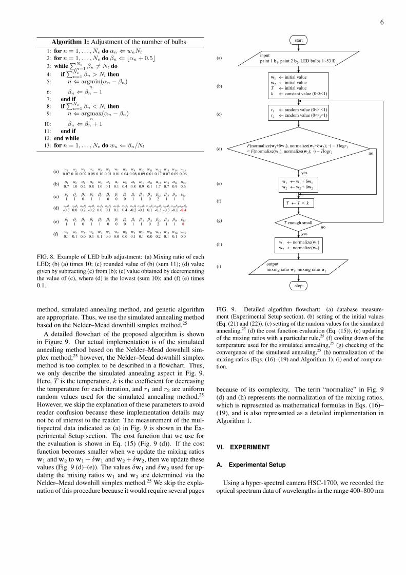
Algorithm 1: Adjustment of the number of bulbs1: for n = 1, . . . , Ne do αn ⇐ wnNl

2: for n = 1, . . . , Ne do βn ⇐ �αn + 0.5�3: while

∑Nen=1 βn �= Nl do

4: if∑Ne

n=1 βn > Nl then5: n ⇐ argmin

n(αn − βn)

6: βn ⇐ βn − 17: end if8: if

∑Nen=1 βn < Nl then

9: n ⇐ argmaxn

(αn − βn)

10: βn ⇐ βn + 111: end if12: end while13: for n = 1, . . . , Ne do wn ⇐ βn/Nl

FIG. 8. Example of LED bulb adjustment: (a) Mixing ratio of eachLED; (b) (a) times 10; (c) rounded value of (b) (sum 11); (d) valuegiven by subtracting (c) from (b); (e) value obtained by decrementingthe value of (c), where (d) is the lowest (sum 10); and (f) (e) times0.1.

method, simulated annealing method, and genetic algorithmare appropriate. Thus, we use the simulated annealing methodbased on the Nelder–Mead downhill simplex method.25

A detailed flowchart of the proposed algorithm is shownin Figure 9. Our actual implementation is of the simulatedannealing method based on the Nelder–Mead downhill sim-plex method;25 however, the Nelder–Mead downhill simplexmethod is too complex to be described in a flowchart. Thus,we only describe the simulated annealing aspect in Fig. 9.Here, T is the temperature, k is the coefficient for decreasingthe temperature for each iteration, and r1 and r2 are uniformrandom values used for the simulated annealing method.25

However, we skip the explanation of these parameters to avoidreader confusion because these implementation details maynot be of interest to the reader. The measurement of the mul-tispectral data indicated as (a) in Fig. 9 is shown in the Ex-perimental Setup section. The cost function that we use forthe evaluation is shown in Eq. (15) (Fig. 9 (d)). If the costfunction becomes smaller when we update the mixing ratiosw1 and w2 to w1+ δw1 and w2+ δw2, then we update thesevalues (Fig. 9 (d)–(e)). The values δw1 and δw2 used for up-dating the mixing ratios w1 and w2 are determined via theNelder–Mead downhill simplex method.25 We skip the expla-nation of this procedure because it would require several pages

FIG. 9. Detailed algorithm flowchart: (a) database measure-ment (Experimental Setup section), (b) setting of the initial values(Eq. (21) and (22)), (c) setting of the random values for the simulatedannealing,25 (d) the cost function evaluation (Eq. (15)), (e) updatingof the mixing ratios with a particular rule,25 (f) cooling down of thetemperature used for the simulated annealing,25 (g) checking of theconvergence of the simulated annealing,25 (h) normalization of themixing ratios (Eqs. (16)–(19) and Algorithm 1), (i) end of computa-tion.

because of its complexity. The term “normalize” in Fig. 9(d) and (h) represents the normalization of the mixing ratios,which is represented as mathematical formulas in Eqs. (16)–(19), and is also represented as a detailed implementation inAlgorithm 1.

VI. EXPERIMENT

A. Experimental Setup

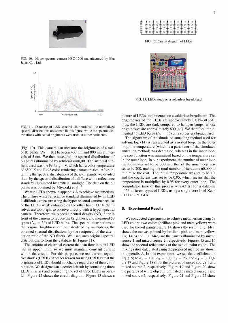
Using a hyper-spectral camera HSC-1700, we recorded theoptical spectrum data of wavelengths in the range 400–800 nm

7

FIG. 10. Hyper-spectral camera HSC-1700 manufactured by EbaJapan Co., Ltd.

Wavelength [nm]400 8000

0.7

Spectral radiance[norm

alized]

FIG. 11. Database of LED spectral distributions: the normalizedspectral distributions are shown in this figure, while the spectral dis-tributions with actual brightness were used in our experiments.

(Fig. 10). This camera can measure the brightness of a totalof 81 bands (Nb = 81) between 400 nm and 800 nm at inter-vals of 5 nm. We then measured the spectral distributions ofoil paints illuminated by artificial sunlight. The artificial sun-light used was the Probright V, which has a color temperatureof 6500 K and Ra98 color-rendering characteristics. After ob-taining the spectral distributions of these oil paints, we dividedthem by the spectral distribution of a diffuse white reflectancestandard illuminated by artificial sunlight. The data on the oilpaints was obtained by Miyazaki et al.15

We use LEDs shown in appendix A to achieve metamerism.The diffuse white reflectance standard illuminated by an LEDis difficult to measure using the hyper-spectral camera becauseof the LED’s weak radiance; on the other hand, LEDs them-selves are too bright to observe directly with a hyper-spectralcamera. Therefore, we placed a neutral density (ND) filter infront of the camera to reduce the brightness, and measured 53types (Ne = 53) of LED bulbs. The spectral distributions atthe original brightness can be calculated by multiplying theobtained spectral distributions by the reciprocal of the atten-uation ratio of the ND filters. We used such original spectraldistributions to form the database E (Figure 11).

The amount of electrical current that can flow into an LEDhas an upper limit, so we must maintain constant currentwithin the circuit. For this purpose, we use current regula-tive diodes (CRDs). Another reason for using CRDs is that thebrightness of LEDs should not change regardless of their com-bination. We designed an electrical circuit by connecting threeLEDs in series and connecting the set of three LEDs in paral-lel. Figure 12 shows the circuit diagram. Figure 13 shows a

FIG. 12. Circuit diagram of LEDs

FIG. 13. LEDs stuck on a solderless breadboard

picture of LEDs implemented on a solderless breadboard. Thebrightnesses of the LEDs are approximately 0.015–30 [cd];thus, the LEDs are dark compared to halogen lamps, whosebrightnesses are approximately 800 [cd]. We therefore imple-mented 45 LED bulbs (Nl = 45) on a solderless breadboard.

The algorithm of the simulated annealing method used forsolving Eq. (14) is represented as a nested loop. In the outerloop, the temperature (which is a parameter of the simulatedannealing method) was decreased, whereas in the inner loop,the cost function was minimized based on the temperature setin the outer loop. In our experiment, the number of outer loopiterations was set to be 300 and that of the inner loop wasset to be 200, making the total number of iterations 60,000 tominimize the cost. The initial temperature was set to be 10,and the coefficient was set to be 0.95, which means that thetemperature is multiplied by 0.95 for every outer loop. Thecomputation time of this process was 43 [s] for a databaseof 53 different types of LEDs, using a single-core Intel XeonCPU at 2.50 GHz.

B. Experimental Results

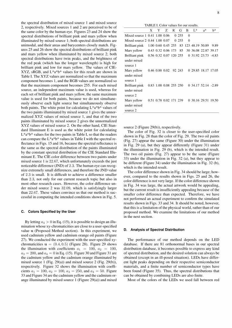
We conducted experiments to achieve metamerism using 53LED colors; two colors (brilliant pink and mars yellow) wereused for the oil paints Figure 14 shows the result. Fig. 14(a)shows the canvas painted by brilliant pink and mars yellow.Fig. 14(b) and Fig. 14(c) are the canvas illuminated by mixedsource 1 and mixed source 2, respectively. Figures 15 and 16show the spectral reflectances of the two oil paint colors. Themixing ratios calculated using the proposed method are shownin appendix A. In this experiment, we set the coefficients inEq. (15) to a1 = 100, a2 = 100, a3 = 25, and a4 = 0. Fig-ure 17 and Figure 18 show the pictures of mixed source 1 andmixed source 2, respectively. Figure 19 and Figure 20 showthe pictures of white object illuminated by mixed source 1 andmixed source 2, respectively. Figure 21 and Figure 22 show

8

the spectral distribution of mixed source 1 and mixed source2, respectively. Mixed sources 1 and 2 are perceived to be ofthe same color by the human eye. Figures 23 and 24 show thespectral distributions of brilliant pink and mars yellow whenilluminated by mixed source 1; both spectral distributions areunimodal, and their areas and barycenters closely match. Fig-ures 25 and 26 show the spectral distributions of brilliant pinkand mars yellow when illuminated by mixed source 2; bothspectral distributions have twin peaks, and the brightness ofthe red peak (which has the longer wavelength) is high forbrilliant pink and low for mars yellow. The values of CIE-XYZ, sRGB, and L*a*b* values for this result are shown inTable I. The XYZ values are normalized so that the maximumcomponent becomes 1, and the RGB values are normalized sothat the maximum component becomes 255. For each mixedsource, an independent maximum value is used, whereas foreach set of brilliant pink and mars yellow, the same maximumvalue is used for both paints, because we do not simultane-ously observe each light source but simultaneously observeboth paints. The white point for calculating L*a*b* values ofthe two paints illuminated by mixed source 1 gives the unnor-malized XYZ values of mixed source 1, and that of the twopaints illuminated by mixed source 2 gives the unnormalizedXYZ values of mixed source 2. On the other hand, CIE Stan-dard Illuminant E is used as the white point for calculatingL*a*b* values for the two paints in Table I, so that the readerscan compare the L*a*b* values in Table I with the spectral re-flectance in Figs. 15 and 16, because the spectral reflectance isthe same as the spectral distribution of the paints illuminatedby the constant spectral distribution of the CIE Standard Illu-minant E. The CIE color difference between two paints undermixed source 1 is 22.67, which unfortunately exceeds the justnoticeable difference (JND) of 2.3. The human eye can recog-nize extremely small differences, and therefore the JND valueof 2.3 is small. It is difficult to achieve a difference smallerthan 2.3, not only for our current research topic but also inmost other research cases. However, the color difference un-der mixed source 2 was 32.09, which is satisfyingly largerthan 22.67. These values convince us that our method is suc-cessful in computing the intended conditions shown in Fig. 5.

C. Colors Specified by the User

By letting a4 > 0 in Eq. (15), it is possible to design an illu-mination whose xy-chromaticities are close to a user-specifiedvalue u (Proposed Method section). In this experiment, weused cadmium yellow and cadmium orange oil paints (Figure27). We conducted the experiment with the user-specified xy-chromaticities u = (0.4, 0.5) (Figure 28). Figure 29 showsthe illumination with coefficients a1 = 100, a2 = 100,a3 = 200, and a4 = 0 in Eq. (15). Figure 30 and Figure 31 arethe cadmium yellow and the cadmium orange illuminated bymixed source 1 (Fig. 29(a)) and mixed source 2 (Fig. 29(b)),respectively. Figure 32 shows the illumination with coeffi-cients a1 = 100, a2 = 100, a3 = 250, and a4 = 50. Figure33 and Figure 34 are the cadmium yellow and the cadmium or-ange illuminated by mixed source 1 (Figure 29(a)) and mixed

TABLE I. Color values for our results.X Y Z R G B L* a* b*

Mixed source 1 0.41 1.00 0.06 0 255 0Mixed source 2 0.44 1.00 0.07 0 255 0Brilliant pink 1.00 0.60 0.45 255 83 123 48.19 50.89 9.89Mars yellow 0.43 0.32 0.06 173 85 30 36.08 22.87 39.17Brilliant pink 0.56 0.32 0.07 120 255 0 31.92 23.73 -4.83under mixedsource 1Mars yellow 0.46 0.88 0.02 92 243 0 29.85 18.17 17.05under mixedsource 1Brilliant pink 0.83 1.00 0.08 255 250 0 34.17 52.14 -2.89under mixedsource 2Mars yellow 0.51 0.78 0.02 171 239 0 30.16 29.51 19.50under mixedsource 2

source 2 (Figure 29(b)), respectively.The color of Fig. 32 is closer to the user-specified color

shown in Fig. 28 than the color of Fig. 29. The two oil paints(Fig. 27) appear the same (Figure 30) under the illuminationin Fig. 29 (a), but they appear differently (Figure 31) underthe illumination in Fig. 29 (b), which is the intended result.The two oil paints (Fig. 27) appear to be the same (Figure33) under the illumination in Fig. 32 (a), but they appear tobe different (Figure 34) under the illumination in Fig. 32 (b),which is the intended result.

The color difference shown in Fig. 34 should be large; how-ever, compared to the results shown in Figs. 25 and 26, thecolor difference is not very large. If the color difference shownin Fig. 34 was large, the actual artwork would be appealing,but the current result is insufficiently appealing because of thesmaller color difference than expected. Therefore, we havenot performed an actual experiment to confirm the simulatedresults shown in Figs. 33 and 34. It should be noted, however,that this is a limitation of the physical world, rather than of ourproposed method. We examine the limitations of our methodin the next section.

D. Analysis of Spectral Distribution

The performance of our method depends on the LEDdatabase. If there are 81 orthonormal bases in our spectraldistribution database, it becomes possible to express any kindof spectral distribution, and the desired solution can always beobtained (except in an ill-posed situation). LEDs have differ-ent light peaks depending on their respective semiconductormaterials, and a finite number of semiconductor types havebeen found (Figure 35). Thus, the spectral distributions thatcan be obtained by combining LEDs are also finite.

Most of the colors of the LEDs we used fall between red

9

(a) (b) (c)

FIG. 14. Experimental result: (a) two types of oil paint, (b) appearance under mixed source 1, and (c) appearance under mixed source 2.

Wavelength [nm] 8004000

0.7

Spectral reflectance[no unit]

Wavelength [nm] 8004000

0.7

Spectral reflectance[no unit]

FIG. 15. Spectral reflectanceof brilliant pink.

FIG. 16. Spectral reflectanceof mars yellow.

FIG. 17. The appearance ofmixed source 1.

FIG. 18. The appearance ofmixed source 2.

and yellow (Fig. 11), but there are only a few kinds of LEDsfor green and blue in our LED database. The purpose of ourresearch is to evaluate the basic framework of computer-aidedart, which designs the illumination under the user-specifieddatabase. We have used many easily obtainable LEDs for the

FIG. 19. The RGB color ofmixed source 1.

FIG. 20. The RGB color ofmixed source 2.

Wavelength [nm]400 8000

45000

Spectral radiance[W

/sr/m2/nm

with

unknown scale]

Wavelength [nm]400 8000

250000

Spectral radiance[W

/sr/m2/nm

with

unknown scale]

FIG. 21. The spectral distribu-tion of mixed source 1.

FIG. 22. The spectral distribu-tion of mixed source 2.

Wavelength [nm]400 8000

3000

Spectral radiance[W

/sr/m2/nm

with

unknown scale]

Wavelength [nm]400 8000

3000

Spectral radiance[W

/sr/m2/nm

with

unknown scale]

FIG. 23. The spectral distri-bution of brilliant pink undermixed source 1.

FIG. 24. The spectral distri-bution of mars yellow undermixed source 1.

database so that, in general, people can design their desiredillumination to create metameric artwork. Because LEDs arecommonly obtainable products and are not custom-made, theycan produce only a limited number of unique spectral distri-butions.

By analyzing the spectral distribution database, it is possi-ble to understand how many basis functions are required to de-scribe the distribution.15,26–31 Because LEDs are narrow-bandsources, they are not suited for principal component analysis;nevertheless, we followed previous works15,26–31 and used thismethod. Although the orthogonal bases computed by princi-pal component analysis do not resemble the spectral distribu-tions of actual LEDs, we can examine the statistical behaviorof our database. Because the results of our methods depend

10

Wavelength [nm]400 8000

20000

Spectral radiance[W

/sr/m2/nm

with

unknown scale]

Wavelength [nm]400 8000

20000

Spectral radiance[W

/sr/m2/nm

with

unknown scale]

FIG. 25. The spectral distri-bution of brilliant pink undermixed source 2.

FIG. 26. The spectral distri-bution of mars yellow undermixed source 2.

(a) (b)

R: 254G: 128B: 0

R: 206G: 55B: 31

R: 235G: 254B: 66

FIG. 27. The RGB colors ofcadmium yellow and cadmiumorange.

FIG. 28. The RGB colors ofxy-chromaticity specified bythe user.

strongly on the database, we regard this analysis as important.Principal component analysis is used for simply understand-ing the rough characteristics of the database, and further de-tailed analysis is not necessary for our method.

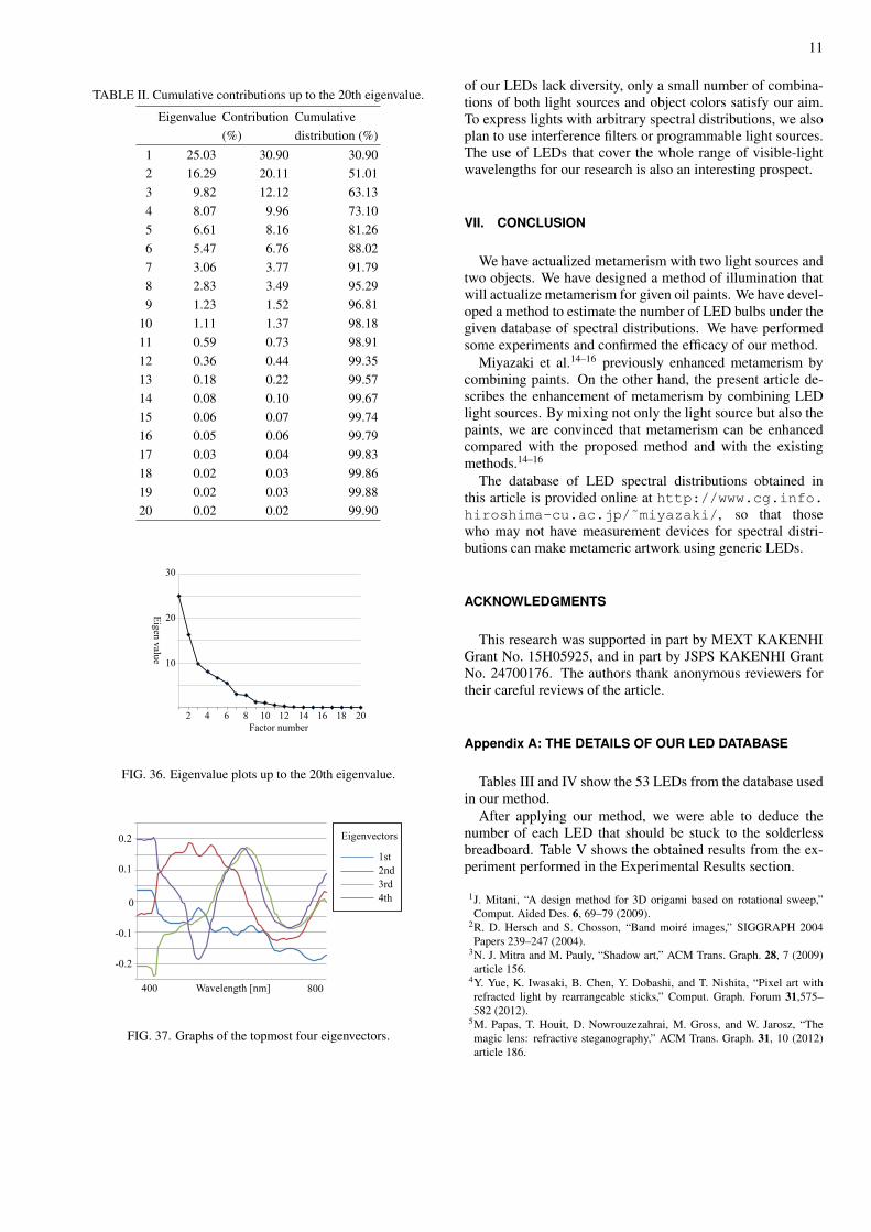
Table II shows the top 20 eigenvalues of the top 20 contri-butions, and the cumulative contributions obtained by princi-pal component analysis for a database with 53 types of LEDs.Figure 36 shows a graph of the top 20 eigenvalues and Figure

(a) (b)

R: 0G: 106B: 253

R: 72G: 91B: 253

FIG. 29. The RGB color of il-lumination calculated withoutuser specification: (a) mixedsource 1, and (b) mixed source2.

(a) (b)

R: 254G: 55B: 157

R: 229G: 0B: 153

(a) (b)

R: 253G: 122B: 105

R: 187G: 72B: 108

FIG. 30. Mixed source 1 cal-culated without user specifica-tion: (a) cadmium yellow and(b) cadmium orange.

FIG. 31. Mixed source 2 cal-culated without user specifica-tion: (a) cadmium yellow and(b) cadmium orange.

(a) (b)

R: 253G: 202B: 108

R: 253G: 202B: 103

FIG. 32. The RGB colorsof illumination calculated withuser specification: (a) mixedsource 1, and (b) mixed source2.

(a) (b)

R: 253G: 0B: 35

R: 238G: 0B: 36

(a) (b)

R: 254G: 119B: 0

R: 198G: 62B: 0

FIG. 33. Mixed source 1 cal-culated with user specification:(a) cadmium yellow and (b)cadmium orange.

FIG. 34. Mixed source 2 cal-culated with user specification:(a) cadmium yellow and (b)cadmium orange.

AlInGaN

InGaN

AlPAlAs

GaPInN

AlInGaP

AlGaAs

400 800Wavelength [nm]

FIG. 35. Colors depending on compounds.

37 shows the top four eigenvectors. As shown in Table II, thecumulative contribution reaches 95% at the 8th eigenvalue,99% at the 12th eigenvalue, and more than 99.9% at the 20theigenvalue. From the statistical perspective, if we have 8–12 types of LED with the same spectral distributions as theseeigenvectors, the mixture of these 8–12 LEDs can reproducealmost all of the possible varieties of spectral distributions thatcan be produced using 53 LEDs. However, the shapes of theeigenvectors are different from the actual LEDs, and in addi-tion, negative intensity and negative coefficients cannot occurin the real world; thus, it is difficult to express various spec-tral distributions using only 8–12 types of LED. Therefore, wehave used all 53 LEDs for the database, to allow the design ofas many spectral distributions as possible. However, the LEDswe have used do not cover the whole range of the visible-lightdomain, as is shown in Fig. 11.

Therefore, it is impossible to express an arbitrary spec-tral distribution using actual LEDs. The simulated anneal-ing method comes close to actualizing metamerism, but thesolution is limited by the user-specified constraint, the finitenumber of existing oil paints, and the finite number of LEDsthat have been manufactured. Since the spectral distributions

11

TABLE II. Cumulative contributions up to the 20th eigenvalue.

Eigenvalue Contribution Cumulative(%) distribution (%)

1 25.03 30.90 30.902 16.29 20.11 51.013 9.82 12.12 63.134 8.07 9.96 73.105 6.61 8.16 81.266 5.47 6.76 88.027 3.06 3.77 91.798 2.83 3.49 95.299 1.23 1.52 96.81

10 1.11 1.37 98.1811 0.59 0.73 98.9112 0.36 0.44 99.3513 0.18 0.22 99.5714 0.08 0.10 99.6715 0.06 0.07 99.7416 0.05 0.06 99.7917 0.03 0.04 99.8318 0.02 0.03 99.8619 0.02 0.03 99.8820 0.02 0.02 99.90

30

Eigen valueFactor number

2 4 6 8 20

20

10

10 12 14 16 18

FIG. 36. Eigenvalue plots up to the 20th eigenvalue.

0.2

400 Wavelength [nm] 800

0.1

0

-0.1

-0.2

Eigenvectors

1st2nd3rd4th

FIG. 37. Graphs of the topmost four eigenvectors.

of our LEDs lack diversity, only a small number of combina-tions of both light sources and object colors satisfy our aim.To express lights with arbitrary spectral distributions, we alsoplan to use interference filters or programmable light sources.The use of LEDs that cover the whole range of visible-lightwavelengths for our research is also an interesting prospect.

VII. CONCLUSION

We have actualized metamerism with two light sources andtwo objects. We have designed a method of illumination thatwill actualize metamerism for given oil paints. We have devel-oped a method to estimate the number of LED bulbs under thegiven database of spectral distributions. We have performedsome experiments and confirmed the efficacy of our method.

Miyazaki et al.14–16 previously enhanced metamerism bycombining paints. On the other hand, the present article de-scribes the enhancement of metamerism by combining LEDlight sources. By mixing not only the light source but also thepaints, we are convinced that metamerism can be enhancedcompared with the proposed method and with the existingmethods.14–16

The database of LED spectral distributions obtained inthis article is provided online at http://www.cg.info.hiroshima-cu.ac.jp/˜miyazaki/, so that thosewho may not have measurement devices for spectral distri-butions can make metameric artwork using generic LEDs.

ACKNOWLEDGMENTS

This research was supported in part by MEXT KAKENHIGrant No. 15H05925, and in part by JSPS KAKENHI GrantNo. 24700176. The authors thank anonymous reviewers fortheir careful reviews of the article.

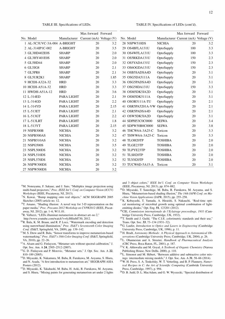
Appendix A: THE DETAILS OF OUR LED DATABASE

Tables III and IV show the 53 LEDs from the database usedin our method.

After applying our method, we were able to deduce thenumber of each LED that should be stuck to the solderlessbreadboard. Table V shows the obtained results from the ex-periment performed in the Experimental Results section.

1J. Mitani, “A design method for 3D origami based on rotational sweep,”Comput. Aided Des. 6, 69–79 (2009).

2R. D. Hersch and S. Chosson, “Band moire images,” SIGGRAPH 2004Papers 239–247 (2004).

3N. J. Mitra and M. Pauly, “Shadow art,” ACM Trans. Graph. 28, 7 (2009)article 156.

4Y. Yue, K. Iwasaki, B. Chen, Y. Dobashi, and T. Nishita, “Pixel art withrefracted light by rearrangeable sticks,” Comput. Graph. Forum 31,575–582 (2012).

5M. Papas, T. Houit, D. Nowrouzezahrai, M. Gross, and W. Jarosz, “Themagic lens: refractive steganography,” ACM Trans. Graph. 31, 10 (2012)article 186.

12

TABLE III. Specifications of LEDs.

Max forward ForwardNo. Model Manufacturer Current (mA) Voltage (V)

1 AL-5C3UVC-3A-004 A-BRIGHT 20 3.22 AL-314IP1C-002 A-BRIGHT 20 3.53 GL3HD402E0S SHARP 20 2.04 GL3HY401E0S SHARP 20 2.05 GL5HD44 SHARP 20 2.06 GL5JG8 SHARP 20 2.17 GL5PR8 SHARP 20 2.18 GL5UR2K1 SHARP 20 1.859 HCEH-A32A-32 HRD 20 3.3

10 HCEH-A51A-32 HRD 20 3.311 HWDH-A51A-12 HRD 20 3.612 L-314ED PARA LIGHT 20 2.113 L-314GD PARA LIGHT 20 2.214 L-314YD PARA LIGHT 20 2.1515 L-513ET PARA LIGHT 20 2.116 L-513GT PARA LIGHT 20 2.217 L-513LRT PARA LIGHT 20 1.818 L-513YT PARA LIGHT 20 2.1519 NSPB300B NICHIA 20 3.220 NSPB500AS NICHIA 20 3.221 NSPB510AS NICHIA 20 3.222 NSPG500S NICHIA 20 3.523 NSPL500DS NICHIA 20 3.224 NSPL510DS NICHIA 20 3.225 NSPL570DS NICHIA 20 3.226 NSPW300DS NICHIA 20 3.227 NSPW500DS NICHIA 20 3.2

6M. Nonoyama, F. Sakaue, and J. Sato, “Multiplex image projection usingmulti-band projectors,” Proc. IEEE Int’l. Conf. on Computer Vision (ICCV)Workshops (IEEE, Piscataway, NJ, 2013).

7N. Kawai, “Bump mapping onto real objects,” ACM SIGGRAPH 2005Sketches (2005) article no. 12.

8T. Amano, “Shading illusion: A novel way for 3-D representation on thepaper media,” Proc. Procams 2012 Workshop on CVPR2012 (IEEE, Piscat-away, NJ, 2012), pp. 1–6, W11 01.

9R. Valluzzi, “LEDs illuminat metamerism in abstract art–no 2,”http://www.youtube.com/watch?v=fyJHlinM730, 2012.

10R. Bala, K. M. Braun, and R. P. Loce, “Watermark encoding and detectionusing narrowband illumination,” Proc. IS&T’s Seventeenth Color ImagingConf. (IS&T, Springfield, VA, 2009), pp. 139–142.

11M. S. Drew and R. Bala, “Sensor transforms to improve metamerism-basedwatermarking,” Proc. IS&T’s 18th Color Imaging Conf. (IS&T, Springfield,VA, 2010), pp. 22–26.

12A. Alsam and G. Finlayson, “Metamer sets without spectral calibration,” J.Opt. Soc. Am. A 24, 2505–2512 (2007).

13G. D. Finlayson and P. Morovic, “Metamer sets,” J. Opt. Soc. Am. A 22,810–189 (2005).

14D. Miyazaki, K. Nakamura, M. Baba, R. Furukawa, M. Aoyama, S. Hiura,and N. Asada, “A first introduction to metamerism art,” SIGGRAPH ASIAPosters (2012).

15D. Miyazaki, K. Takahashi, M. Baba, H. Aoki, R. Furukawa, M. Aoyama,and S. Hiura, “Mixing paints for generating metamerism art under 2 lights

TABLE IV. Specifications of LEDs (cont’d).

Max forward ForwardNo. Model Manufacturer Current (mA) Voltage (V)28 NSPW510DS NICHIA 20 3.229 OS4BFLA131U OptoSupply 100 3.330 OS4WFLA131U OptoSupply 100 3.331 OS5RKDA131U OptoSupply 150 2.332 OS5YADA131U OptoSupply 150 2.333 OS6OGDA131U OptoSupply 150 2.334 OSB5SADSA4D OptoSupply 20 3.135 OSG5DA5111A OptoSupply 20 3.136 OSG5PADSA4D OptoSupply 20 3.137 OSG58DA131U OptoSupply 150 3.338 OSM5DK5JA2D OptoSupply 20 3.139 OSM5DK5111A OptoSupply 20 3.140 OSOR5111A-TU OptoSupply 20 2.141 OSR5PA5201A-VW OptoSupply 20 2.142 OSR5PADSA4D OptoSupply 20 2.143 OSW5DK5JA2D OptoSupply 20 3.144 SDPH53C0C0000 SEIWA 20 3.445 SDPW50B0C0000 SEIWA 20 3.846 THCW6A-3A25-C Toricon 20 3.347 THWW6A-3A25-C Toricon 20 3.348 TLOH20TP TOSHIBA 20 2.049 TLGE23TP TOSHIBA 20 2.050 TLPYE23TP TOSHIBA 20 2.051 TLSH20TP TOSHIBA 20 2.052 TLYH20TP TOSHIBA 20 2.053 TUCW6D-5A15-A Toricon 20 3.1

and 3 object colors,” IEEE Int’l. Conf. on Computer Vision Workshops(IEEE, Piscataway, NJ, 2013), pp. 874–882.

16D. Miyazaki, T. Saneshige, M. Baba, R. Furukawa, M. Aoyama, and S.Hiura, “Metamerism-based shading illusion,” The 14th IAPR Conf. on Ma-chine Vision Applications (IAPR, 2015), pp. 255–258.

17K. Kobayashi, T. Yamada, A. Hiraishi, S. Nakauchi, “Real-time opti-cal monitoring of microbial growth using optimal combination of light-emitting diodes,” Opt. Eng. 51, 123201 (2012).

18CIE, Commission internationale de l’Eclairage proceedings, 1931 (Cam-bridge University Press, Cambridge, UK, 1932).

19T. Smith and J. Guild, “The C.I.E. colorimetric standards and their use,”Trans. Opt. Soc. 33, 73–134 (1931–32).

20G. Laufer, Introduction to Optics and Lasers in Engineering (CambridgeUniversity Press, Cambridge, UK, 1996), p. 11.

21H. Bradt, Astronomy Methods: A Physical Approach to Astronomical Ob-servations (Cambridge University Press, Cambridge, UK, 2004), p. 26.

22L. Ohannesian and A. Streeter, Handbook of Pharmaceutical Analysis(CRC Press, Boca Raton, FL, 2001), p. 187.

23V. K. Ahluwalia and M. Goyal, A Textbook of Organic Chemistry (NarosaPublishing House, New Delhi, 2000), p. 110.

24L. Simonot and M. Hebert, “Between additive and subtractive color mix-ings: intermediate mixing models,” J. Opt. Soc. Am. A 31, 58–66 (2014).

25W. H. Press, S. A. Teukolsky, W. T. Vetterling, and B. P. Flannery, Numer-ical Recipes in C: the Art of Scientific Computing (Cambride UniversityPress, Cambridge, 1997), p. 994.

26D. B. Judd, D. L. MacAdam, and G. W. Wyszecki, “Spectral distribution of

13

TABLE V. Mixing ratios (number of LEDs).

No. LED Light 1 Light 2 No. LED Light 1 Light 21 AL-5C3UVC-3A-004 0 0 28 NSPW510DS 0 02 AL-314IP1C-002 0 0 29 OS4BFLA131U 0 03 GL3HD402E0S 0 2 30 OS4WFLA131U 0 04 GL3HY401E0S 0 0 31 OS5RKDA131U 0 75 GL5HD44 0 0 32 OS5YADA131U 0 06 GL5JG8 3 1 33 OS6OGDA131U 0 07 GL5PR8 0 0 34 OSB5SADSA4D 0 08 GL5UR2K1 0 0 35 OSG5DA5111A 0 289 HCEH-A32A-32 0 0 36 OSG5PADSA4D 0 1

10 HCEH-A51A-32 0 0 37 OSG58DA131U 41 211 HWDH-A51A-12 0 0 38 OSM5DK5JA2D 0 012 L-314ED 0 0 39 OSM5DK5111A 0 013 L-314GD 0 0 40 OSOR5111A-TU 0 114 L-314YD 0 0 41 OSR5PA5201A-VW 0 015 L-513ET 0 0 42 OSR5PADSA4D 0 216 L-513GT 1 0 43 OSW5DK5JA2D 0 017 L-513LRT 0 0 44 SDPH53C0C0000 0 018 L-513YT 0 0 45 SDPW50B0C0000 0 019 NSPB300B 0 0 46 THCW6A-3A25-C 0 020 NSPB500AS 0 0 47 THWW6A-3A25-C 0 021 NSPB510AS 0 0 48 TLOH20TP 0 022 NSPG500S 0 0 49 TLGE23TP 0 023 NSPL500DS 0 0 50 TLPYE23TP 0 124 NSPL510DS 0 0 51 TLSH20TP 0 025 NSPL570DS 0 0 52 TLYH20TP 0 026 NSPW300DS 0 0 53 TUCW6D-5A15-A 0 027 NSPW500DS 0 0

typical daylight as a function of correlated color temperature,” J. Opt. Soc.Am. 54, 1031–1040 (1964).

27J. P. S. Parkkinen, J. Hallikainen, and T. Jaaskelainen, “Characteristic spec-tra of Munsell colors,” J. Opt. Soc. Am. A 6, 318–322 (1989).

28J. Cohen, “Dependency of the spectral reflectance curves of the Munsellcolor chips,” Psychonomical Sci. 1, 369–370 (1964).

29L. T. Maloney, “Evaluation of linear models of surface spectral reflectance

with small numbers of parameters,” J. Opt. Soc. Am. A 10, 1673–1683(1986).

30M. J. Vrhel, R. Gershon, and L. S. Iwan, “Measurement and analysis ofobject reflectance spectral,” Color Res. Appl. 19, 4–9 (1994).

31S. Tominaga and N. Tanaka, “Spectral image acquisition, analysis, and ren-dering for art paintings,” J. Electron. Imaging 17, 043022 (2008).