Optimization of Insecticide Allocation for Kala-Azar … AND OTHERS OPTIMIZATION FOR KA CONTROL IN...

GORAHAVA AND OTHERS OPTIMIZATION FOR KA CONTROL IN BIHAR

1

Optimization of Insecticide Allocation for Kala-Azar Control in Bihar, India

Kaushik K. Gorahava1, Anuj Mubayi

2, and Jay M. Rosenberger

1

1Industrial and Manufacturing Systems Engineering Department, The University of Texas at Arlington, Arlington,

Texas; 2Department of Mathematics, Northeastern Illinois University, Chicago, Illinois;

Department of

Mathematics, The University of Texas at Arlington, Arlington, Texas; Mathematical Computational and Science

Center, Arizona State University, Phoenix, Arizona

Abstract. The visceral form is the most deadly form of the leishmaniasis family, which affects

poor and developing countries. The Indian state of Bihar has the highest prevalence and

mortality rate due to visceral leishmaniasis in the world, where it is also referred to as Kala-Azar.

Insecticide spraying is the current vector control procedure for controlling its spread in Bihar.

This study proposes a novel optimization model in order to identify an optimal allocation of

insecticide (DDT or Deltamethrin) based on the sizes of both human and cattle populations. As

an example, DDT and Deltamethrin have been compared using the model. The model maximizes

the insecticide-induced death rate caused by spraying human and cattle dwellings given the

limited financial resources available to the public health department. The results suggest that

until the first 90 days after spraying, DDT yields more than three times the insecticide-induced

death rate achieved by Deltamethrin in the absence of any insecticide resistance. The study

implies that ignoring the resistance developed by sandflies to DDT, Deltamethrin might not be a

good replacement for DDT. The study also confirms that the present practice of first spraying

houses to optimize sandfly mortality ahead of spraying cattle sites is appropriate.


2

INTRODUCTION

Visceral leishmaniasis (VL) is a sandfly-borne infectious disease that is fatal if left untreated.1

Known as Kala-Azar in India, it is transmitted to the human population when an infected female

sandfly bites a susceptible human and transmits the parasite Leishmania donovani. Male

sandflies are also known to feed on blood,2 and blood is a crucial source of protein and iron for

female sandflies to develop eggs. Phlebotomus argentipes (a sandfly species) is the primary

vector of L. donovani in southern Asia3 including India. India, an agricultural country, has a

sizable cattle population that is frequently visited by sandflies for mating and feeding purposes.

The blood-feeding preferences of different sandfly species have been well documented in the

literature. An investigation of the stomach contents of P. argentipes from six districts of North

Bihar showed that blood-fed female sandflies have a preference for bovine blood (68%),

followed by human blood (18%), and avian blood (4%)4, hence showing them to be zoopholic.

Furthermore, an examination of soil samples in Bihar showed that P. argentipes has a higher

tendency to breed in the alkaline soil of cattle sheds than in soil that has a neutral pH found in

human houses.5 Cattle sheds, where the soil might have a high content of moisture and organic

matter such as cow dung, provide an ideal breeding site for P. argentipes.6 The foregoing

discussion verifies the importance of considering cattle sites in insecticide residual spraying

efforts. Previous studies7 showed that spraying cattle sheds in Brazil caused increased sandfly

density in unprotected human dwellings. Therefore, we develop a model that focuses on

insecticide spraying programs in both human and cattle sites.

The burden of VL in terms of disability-adjusted life years lost in India was estimated in 1990 to

be 0.5 million and 0.68 million for women and men, respectively.8 The average number of

annual VL cases in India between 2004 and 2008 was reported to be 34,918, although this total


3

dropped to 28,382 cases in 2010.9 The provisional number of Kala-Azar cases in India in 2011

was 31,000.10

Given the seriousness of infection, the governments of India, Bangladesh, and

Nepal launched an initiative in 2005 to reduce annual incidences of VL to lower than one per

10,000 persons by 2015.11

As an intervention measure, the Bihar government now carries out

insecticide residual spraying every year starting in February.12

The current policy of the public health department of the Indian state of Bihar considers only the

human population size13

of each district for computing the amount of insecticide (presently

DDT) to be allocated for spraying. The cattle population in a district is not included in these

insecticide allocation calculations. Because allocating an amount of insecticide to spraying cattle

sheds might control the spread of VL more effectively, a mathematical framework that identifies

an optimal allocation of insecticide based on local human as well as cattle populations would

therefore be valuable. For this purpose, two modeling approaches are presented herein: an

optimization model and a Benefit to Materials Cost Ratio (BMCR) function. The present study

uses these models in order to investigate an optimal allocation of insecticide based on both cattle

and human population sizes.13

Please note that because the BMCR function approach is

completely independent of the optimization model, it provides us with a different perspective on

choosing sites for spraying.

The model developed herein can be used for comparing insecticides considered for future use in

spray campaigns in Bihar. The current insecticide (DDT) residual spray program in Bihar has

been reported to have low effectiveness due to the emergence of P. argentipe’s resistance to

DDT. Replacing DDT by an alternative insecticide has been suggested.14

The model in this study

can thus be used when considering this replacement. The maximum achievable insecticide-


4

induced death rate within the available budget constraint is used as a criterion by the presented

optimization model.

Our results suggest that despite spending approximately Rs. 590 million in spray campaigns,

spraying more sites does not increase the sandfly population’s insecticide-induced death rate

substantially. The model estimates an 18% increase in natural sandfly death rate in Bihar, 90

days after spraying, based on the present insecticide allocation policy. Hence, after covering a

certain spray area, it might be better to invest funds in other sandfly control interventions such as

bed-nets and ecological vector management.15

The remainder of the paper is structured as follows. The Data Sources section describes the data

sources used to estimate the model parameters. The Methods section explains the equations and

assumptions of the three components of the linear optimization model. The Analysis section

presents the analytical results and recommendations for choosing a spray coverage option by

using a BMCR function. The Numerical Results section presents the numerical results derived

from the model. Finally, the Discussion section discusses the implications of the model’s results

and offers suggestions for future ideas to improve the model.

DATA SOURCES

The 1982 Cattle Census16

and 2010--2011 budget allocation document from the public health

department of Bihar13

were used to estimate the sizes of the cattle and human populations in the

VL-affected districts in Bihar, respectively. The average number of cattle per cattle shed in Bihar

was assumed to be the average livestock herd size (number of cow equivalents per household)

from previous studies.17


5

The cost of the insecticide spray campaign was also formulated using data from the 2010--2011

budget document.13

The costs related to materials and implementation (including salaries, spray

equipment, and miscellaneous expenses) were added in order to calculate the total cost of the

insecticide spray campaign. Both the direct and the indirect costs associated with implementation

were used to derive the cost equation (Appendix 3). The data include 354 public health centers

(PHCs) and 10,686 villages.13

Furthermore, the number of occupied residential houses was

estimated for VL-affected districts (excluding data for the Arwal district) from the 1991 Census

of India.18

Financial constraints preclude the spraying of all houses in a district. Because the model

proposed herein aims to optimize the amount of insecticide sprayed per person and per cattle (per

capita hereafter), the two decision variables were set as “kilograms of insecticide allocated per

person” and “kilograms of insecticide allocated per cattle.” When the available budget cannot

procure enough insecticide to cover all sites in the state, it is referred to as a “resource-limited

case” and is used to formulate some of the constraints in the model (Appendix 4).

The natural sandfly death rate was estimated using 2 years of monthly data representing the daily

survival probability of P. papatasi19

. Moreover, the appropriate literature sources were referred

to in order to estimate P. argentipes’s mortality, 24 hours after spraying with DDT20

and

Deltamethrin14

. An insecticide’s lethal effect is assumed to decay exponentially over time.21

The

decay rates inside houses14

and cattle sheds22

were then estimated using data from the literature

(Appendix 1). Previous studies (see the references in Table 1 and Table 2) were also consulted in

order to estimate the epidemiological and demographical parameters for the host and vector

populations.


6

METHODS

The proposed optimization model comprises three components. The first component is the

objective function (Equation 3), which captures the insecticide-induced death rate and which is

maximized in the model. The insecticide-induced death rate is achieved by spraying insecticide

in houses and cattle sheds (derivation in Appendix 2). The decision variables (output from the

model) in the objective function are then the amount of insecticide allocated per person and per

cattle. The demographic parameters used in the objective function as well as in the constraints

are described in Table 1.

Table 1. Demographic parameters for Bihar state

Symbol Definition Unit Estimates :

Mean (SD)

g Number of PHCs in Bihar Number of government clinics 354 13

Nh Size of the human population in the 31 VL-

affected districts in Bihar

Number of humans 33,898,857 13

Nc Size of the cattle population in the 31 VL-

affected districts in Bihar

Number of cattle 21,571,585 16

Nv Size of the sandfly population in Bihar Number of sandflies Assumed constant in the

optimization model

H Total number of houses in Bihar Number of houses 7,933,615 18

Average herd size per cattle shed Number of cattle equivalents 4.6 (2.6) 17

Z =

Number of cattle sheds Number of cattle sheds 4,689,475 16

SD: standard deviation


7

The insecticide toxicity and entomological parameters used in the objective function and in the

constraints are described in Table 2.

Table 2. Insecticide toxicity and entomological parameters

Symbol Definition Unit Estimates

Mean (SD) (95% CI)

ah Female sandflies’ feeding preference for human blood Dimensionless 179.2×10-03 (95% CI, 15.14--20.72) 4

ac = 1 -

ah

Female sandflies’ feeding preference for cattle blood Dimensionless 820.8×10-03 4

Q Human visitation proportion of P. argentipes based on

blood preference

A proportion

between 0 and 1

0.2554 [Estimated in Appendix 1]

Time elapsed after the spray of insecticide Days User-defined value

Per capita death rate of sandflies Sandfly deaths

per day per

sandfly

0.0759 (0.0162) 19

Ih Amount of DDT consumed per 200 m2 house kg per house 533×10-03 23

Ih Amount of Deltamethrin consumed per 200 m2 house kg per house 400×10-03 23

Iz Amount of DDT consumed per cattle shed kg per cattle shed 533×10-03 /2 = 266.5×10-03 23

Iz Amount of Deltamethrin consumed per cattle shed kg per cattle shed 400×10-03 /2 = 200×10-03 23

Ct0 Initial efficacy of DDT (in houses and cattle sheds) Dimensionless 0.54 (95% CI, 48.7--59.3) 20

Ct0 Initial efficacy of Deltamethrin (in houses and cattle

sheds)

Dimensionless 9.75×10-01 14

b1 Decay rate of both insecticides’ lethal effect inside

houses

Fraction per day 0.012 (0.009) (Estimated in Appendix

1, using data from 20)


8

b2 Decay rate of both insecticides’ lethal effect inside

cattle sheds

Fraction per day 0.081 (0.055) (Estimated in Appendix

1, using data from 22)

CI: confidence interval, kg : kilogram

The notations representing the objective function, materials and implementation cost of the spray

campaign, available state budget amount, and per capita allocated amount are described in Table

3.

Table 3. Model’s objective function, budget constraint, and decision variables

Symbol Definition Unit Description

Insecticide-induced death rate of sandflies Sandfly deaths per

day per sandfly

Objective function value obtained from the

model (equation derived in Appendix 2)

(x,y) Total cost of insecticide materials and spray

campaign implementation

Rs. Budget constraint in the model (equation

derived in Appendix 3)

Upper bound on the budget available for the

spray campaign

Rs. User-defined (budget) value in the model

x Insecticide allocated per capita for a 60-day

spray period

kg per person Decision variable value obtained from the

model

y Insecticide allocated per cattle for a 60-day spray

period

kg per cattle Decision variable value obtained from the

model

Rs: Rupees

A parameter termed the “human visitation rate” of mosquitoes24

was used to analyze malaria

transmission dynamics. A similar parameter (human visitation proportion, Q), captured in the

objective function of our model, is used to quantify the proportion of sandflies visiting human

and cattle sites based on the attraction rate of the vector P. argentipes towards the blood of each

host. The feeding behavior of the vector is thus directly incorporated into the model.


9

Temporal exponential functions (h(τ), Equation 1 and z(τ), Equation 2) are used to capture the

deteriorating lethal effect of the insecticide on vectors, and these include parameters such as

decay rate (b1 and b2) and initial efficacy (Ct0).21

The proportions of sandflies that die on the

day after insecticide application inside houses and cattle sheds, respectively, are thereby given

by

( ) ; 1

and

( ) ; . 2

The value of initial efficacy ( ) for both insecticides is assumed to be equal in both houses and

cattle sheds. Figure 1 shows the daily distribution of the sandfly population at sprayed and

unsprayed sites, which depends on the blood meal preference parameter, Q. The objective

function (Equation 3) uses this distribution of the sandfly population. Appendix 2 shows the

derivation of the insecticide-induced death rate (objective function) at sprayed sites on the

day after spraying. Each day, a sandfly either dies a natural death or dies because of the

insecticide’s lethal effect. Note that while the repellent effect of the insecticide is ignored in the

model derivation, we assume that all sandflies that visit a certain insecticide-treated house or

cattle shed are exposed to the insecticide and that a proportion of them die based on the

insecticide’s lethal effect on that day. The term “spray coverage” is thus used in this study to

refer to the number of houses ( ) and cattle sheds ( ) where insecticide is sprayed. Appendix 4

shows the model formulation in terms of x and y only.


10

Figure 1. Distribution of the daily sandfly population based on their blood-feeding

behavior.

The total sandfly death rate is calculated by adding the natural death rate ( ) and the insecticide-

induced death rate ( ) at sprayed sites. The first and second terms of the objective function

(Equation 3) are therefore the insecticide-induced death rates in houses and cattle sheds,

respectively. In the model, the sandfly population size is assumed to be constant.

The second component of the model describes the budget constraint (Equation 4), which

ensures that the total spray campaign cost (materials and implementation in Table 3) is less than

or equal to the available state budget. Furthermore, insecticide applications are assumed to occur

only once per year rather than the existing policy of spraying twice per year in Bihar (derivation

of spray campaign cost equation in Appendix 3).


11

Table 4. Materials and implementation costs related to the insecticide spray campaign

Symbol Materials cost Unit Estimate

Cost per kg of insecticide (DDT) Rs./kg of DDT 90 23

Cost per kg of insecticide (Deltamethrin) Rs./kg of Deltamethrin 810 23

Implementation cost: Personnel and maintenance Unit Estimate

N2 Number of spraying teams or squads allocated per 10 lakh population of

a district

Squads/person 55/106 13

N3 Number of supervisors per squad Number of

supervisors/squad

1 13

N4 Number of field workers per squad Number of workers/squad 5 13

N5 Salary paid to each supervisor/day of the 60-day spray period Rs./day/supervisor 145 13

N6 Salary paid to each field worker/day of the 60-day spray period Rs./day/worker 118 13

N7 Number of days allocated for spraying activity each time spraying is

carried out

Number of days 60 13

N8 Funds allocated per squad for the repair and purchase of spray

equipment per 60-day spray period

Rs./squad/60-day spray

period

950 13

Implementation cost: Operational expenses Unit Estimate

N9 Funds allocated to the district for the transportation of DDT/PHC in the

district (assumed per 60-day spray period)

Rs./ PHC 3500 13

N10 Funds allocated to the district as office expense per squad in the district

(assumed per 60-day spray period)

Rs./squad 250 12

N11 Funds allocated as contingency/squad (assumed per 60-day spray period) Rs./ squad 250 13

N12 Total funds allocated per district for general vehicle mobility/month of

spray period

Rs./ month 20000 13

N13 Funds allocated per district for PHC vehicle mobility/day/PHC for the

60-day spray period

Rs./day/PHC 650 13

N14 Funds allocated for supervision/affected PHC (assumed per 60-day spray

period)

Rs./affected PHC 2000 13

N15 Funds allocated for education and communication activities per affected Rs./affected PHC 2000 13


12

PHC (assumed per 60-day spray period)

Exchange rate in year 2000: 1 USD = INR 45.

The third component consists of the remaining constraints (inequalities 5 to 9) of the model,

which are related to insecticide consumption and sites under the insecticide intervention program

(Appendix 4). As before, it is assumed that the budget is not enough to spray all houses and

cattle sheds during the spray campaign (resource-limited cases).

In the model, only two types of sites are sprayed: human dwellings and cattle sheds (mixed

dwellings do not exist). The other assumptions are: cattle are the only non-human hosts that

sandflies bite; all houses are assumed to have an average area of 200 m2 based on a previous

estimate;23

and the insecticide necessary to spray one cattle shed is assumed to be half that

required to cover one house. Using the three above-described components and their assumptions,

the model can thus be described as follows:

Maximize,

[ ( )] ( * ( )[ ( )] (

* 3

Subject to,

( ) 4

5

(

* 6

7


13

(

* 8

9

ANALYSIS

Optimal solution for the model. This section describes the detailed steps towards finding

possible solutions of the model. Clearly, an optimal solution of the model represents the

allocation of per-capita insecticide at the two sites (decision variables and ) that maximizes

the insecticide-induced death rate. An optimal solution can thus occur at one of the four distinct

points in the feasible domain of the model depending on the conditions based on the model

parameters (Table 5). Table S 5 in the Appendix provides the different abbreviations used in this

paper.

The feasible domain of the insecticide-induced death rate (objective function) (x,y), where

represents the value of the function at point A in the domain, is a 2D region defined by

constraints 4 through 9. The horizontal axis of the feasible domain represents the per-capita

amount of insecticide allocated at house sites (x) and the vertical axis represents the per-capita

amount of insecticide allocated at cattle sites (y).


14

Figure 2. The feasible domain of the optimization model. (a) Case I (Case II) arises when

constraint 4 intersects with constraint 9 (between OC and OE) resulting in point A (point

B) as an optimal solution. (b) Case III (Case IV) arises when constraint 4 intersects with

constraint 9 and constraint 5 (between OC and DE) resulting in point A (point B) as an

optimal solution. (c) Case V (Case VI) arises when constraint 4 intersects with constraint 9

and constraint 7 (between OE and CD) resulting in point A (point B) as an optimal

solution. (d) Case VII (Case VIII) arises when constraint 4 intersects with constraint 5 and

constraint 7 (between DE and CD) resulting in point A (point B) an optimal solution.

Figure 2(a) illustrates Cases I and II (details in Figure 2(a) caption) within which O, A, and B are

the corner points of the feasible domain. An optimal solution in these cases exists at either point


15

A or point B. It is simple to see that the total insecticide-induced death rate at point A is always

less than or equal to the corresponding value at point E, that is, (substituting the

points A and E into Equation 3) or

10

Similarly, the total insecticide-induced death rate at point B is always less than or equal to that at

point C, that is, which simplifies to

11

Case I (if an optimal solution occurs at point A, Figure 2(a)): Since ,

( ) ( )

( )

12

Note that the left-hand side of inequality 12 can be interpreted as the ratio of the insecticide-

induced death rate (( ) ( )) to the insecticide consumed in cattle sheds ( ). Similarly,

the right-hand side of inequality 12 can be interpreted as the same ratio for houses. Hence,

inequality 12 shows that if an optimal solution occurs at point A, then the insecticide-induced

death rate per kilogram of insecticide consumed for houses is greater than the corresponding

ratio for cattle sheds. Inequality 12 thus simplifies to

( ) ( ) ( ) 13

In this case, an optimal solution occurs at point A ( ).

Case II (if an optimal solution occurs at point B, Figure 2(a)): Since ,

( ) ( ) ( ) 14

In this case, an optimal solution occurs at point B ( ). Figure 2(b) illustrates

Cases III and IV (details in Figure 2(b) caption). An optimal solution in these cases exists at

either point A or point B, where it is simple to see , that is,


16

15

In Cases III and IV, satisfies naturally, which simplifies to inequality 11.

Case III (if an optimal solution occurs at point A, Figure 2(b)): In this case,

(inequality 13) and (inequality 15) are obvious to see. Hence, an optimal

solution occurs at point A, as shown in Figure 2(b).

Case IV (if an optimal solution occurs at point B, Figure 2(b)): In this case,

(inequality 14) and (inequality 11). Hence, an optimal solution occurs at point B, as

shown in Figure 2(b). Figure 2(c) illustrates Cases V and VI (details in Figure 2(c) caption). For

these cases, an optimal solution exists only at point A or at point B. and

follow naturally, which simplifies, respectively, to inequality 10 and

16

Case V (if an optimal solution occurs at point A, Figure 2(c)): In this case, (inequality

13) and (inequality 10). Hence, an optimal solution occurs at point A.

Case VI (if an optimal solution occurs at point B, Figure 2(c)): In this case,

(inequality 16) and (inequality 14). Hence, an optimal solution occurs at point B.

Figure 2(d) illustrates Cases VII and VIII (details in Figure 2(d) caption). An optimal solution in

these cases exists only at point A or at point B. It can be seen (inequality 16).

The total insecticide-induced death rate ( ) at points A, E, and D satisfies the inequality:

(inequality 15)

Case VII (if an optimal solution occurs at point A, Figure 2(d)): In this case,

(inequality 15) and (inequality 13), and hence an optimal solution occurs at A.

Case VIII (if an optimal solution occurs at point B, Figure 2(d)): In this case,

(inequality 16) and (inequality 14). Hence, an optimal solution occurs at point B.


17

Since some of these eight cases above result in the same optimal points, the results can be

summarized into four distinct points (Table 5). Each row in this table represents one distinct

optimal solution, the existence of which depends on two conditions (Conditions I and II). An

optimal solution is a function of τ and (refer to Table 2 and Table 3 for the parameter

definitions).

Table 5. Optimal solution for the model

Existence Solution

Symbol

( ( ) ( ))

Condition I Condition II

FS 1

(

)

( )

FS 2

(

)

FS 3

(

)

( )

FS 4

(

)

( ) FS 5 (

*

INFS Infeasible

( ) ( ) ( ) The solution is valid only when both existence conditions are satisfied. A feasible

solution (FS) does not exist (INFS) if .

Therefore, FS 5 (Table 5) implies that surplus money will be left over ( (

( ))) after spraying 100% of both sites (point D in Figure 2). The notations used for

the optimal solution are presented in Table 6.

Table 6. Notations used for the optimal solution

Notation Explanation

FS 1 Spray the maximum possible number of houses with the given budget

FS 2 Spray 100% of houses and then the maximum possible number of cattle sheds with the remaining

budget


18

FS 3 Spray the maximum possible number of cattle sheds with the given budget

FS 4 Spray 100% of cattle sheds and then the maximum possible number of houses with the remaining

budget

FS 5 Spray 100% of houses and cattle sheds

Benefit to Material Cost Ratio. The analysis in this subsection, by using a simple BMCR

function, is developed independent of the optimization model and is used to analyze spray

coverage. The optimization model discussed in the above subsection maximizes the

instantaneous (on the day after spraying) insecticide-induced sandfly death rate within the

available budget. By contrast, the BMCR approach identifies the cumulative number of sandflies

killed (“benefit”) per unit of materials cost until the day after spraying. However, while the

optimization model assumes a constant (Table S 3. in Appendix 2), the BMCR assumes an

exponentially decaying sandfly population.

Using the notation presented in Table 2, the benefit in houses and cattle sheds τ days after

spraying depends on ( ) and ( ). The amount of insecticide consumed for spraying

houses and cattle sheds is and , respectively. The materials cost of spraying

houses and cattle sheds can be expressed as (Rs.) and (Rs.) , respectively.

In the next step, the two contrasting extreme spray coverage options (𝑂 and 𝑂 ) are compared

using the BMCR function. 𝑂 and 𝑂 are the options of spraying insecticide only in 100% houses

(𝑂 : ) and only in 100% cattle sheds (𝑂 : ), respectively.

When houses are sprayed (Equation 3), the insecticide-induced death rate per sandfly on the

day is given by


19

;

17

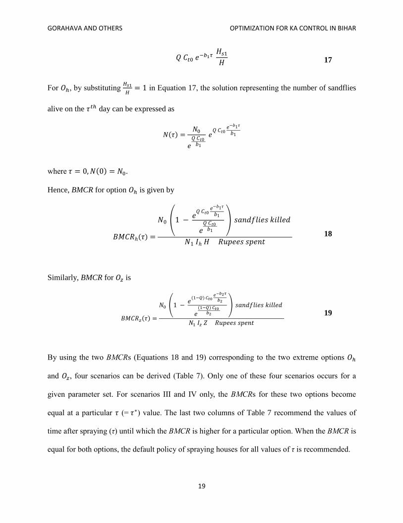
For 𝑂 , by substituting

in Equation 17, the solution representing the number of sandflies

alive on the day can be expressed as

( )

where ( ) .

Hence, BMCR for option 𝑂 is given by

𝐵𝑀 𝑅 ( )

(

)

𝑅𝑢𝑝 𝑝

18

Similarly, BMCR for 𝑂 is

𝐵𝑀 𝑅 ( )

( ( ; )

( ; )

)

𝑅𝑢𝑝 𝑝

19

By using the two BMCRs (Equations 18 and 19) corresponding to the two extreme options 𝑂

and 𝑂 , four scenarios can be derived (Table 7). Only one of these four scenarios occurs for a

given parameter set. For scenarios III and IV only, the BMCRs for these two options become

equal at a particular (= ) value. The last two columns of Table 7 recommend the values of

time after spraying (τ) until which the BMCR is higher for a particular option. When the BMCR is

equal for both options, the default policy of spraying houses for all values of τ is recommended.


20

Table 7. A particular scenario exists if its corresponding pair of parameter conditions is satisfied. For

an existing scenario, one of the two spray options can be selected (knowing that a high BMCR is

desirable τ days after spraying).

Scenario Pair of conditions satisfied Existence of

(when ( )

( ) )

The BMCR is higher in

houses for cattle sheds for

I ( ; ) :

; No

II ( ; ) :

; No

III ( ; ) :

; Yes

IV ( ; ) :

; Yes

Here, V =

and W =

( ; )

;

( ;

; ) and

; -spray coverage of 100% houses; -spray coverage of 100% cattle sheds

Although the discussion below is based on the assumed spray coverage options 𝑂 and 𝑂 , it can

be applied for any values of spray coverage. The foregoing allows us to conclude the following:

Remark 1. In summary, after the first round of spraying (τ = 0), if the aim is to always maintain

a higher BMCR in houses, then scenarios I and II might be helpful. If scenario I exists,

implementing 𝑂 is recommended. If scenario II exists, then implementing 𝑂 is recommended.

Remark 2. If sandfly density peaks days after the first round of spraying (e.g., due to the start

of the rainy season) and a second round of spraying is not possible at time within the available

budget, then it is advisable to implement the spray option that maintains a higher BMCR at time

.

Scenario III (IV) suggests that, for , the BMCR will be higher for 𝑂 (𝑂 ) and that, for

, the BMCR will be higher for 𝑂 (𝑂 ). Thus:

i) If scenario III occurs and days, implementing 𝑂 is recommended, because after

days, the BMCR is higher for 𝑂 (𝐵𝑀 𝑅 ( ) 𝐵𝑀 𝑅 ( ), (implying that by

implementing 𝑂 , a higher reduction in sandfly density per rupee invested will have been


21

achieved in days). However, if day , then implementing 𝑂 is recommended,

because 𝐵𝑀 𝑅 ( ) 𝐵𝑀 𝑅 ( ) .

ii) If scenario IV occurs and days, implementing 𝑂 is recommended, because

𝐵𝑀 𝑅 ( ) 𝐵𝑀 𝑅 ( ). However, if days, then implementing 𝑂 is

recommended, because 𝐵𝑀 𝑅 ( ) 𝐵𝑀 𝑅 ( ) .

NUMERICAL RESULTS

This section compares the impact on the sandfly death rate of the two studied insecticides (DDT

and Deltamethrin) by developing and analyzing a deterministic optimization model. The

estimates of certain model parameters for Bihar are not available in the literature. This study thus

estimates and provides a procedure to extract information on these parameters indirectly by using

the available data. The estimates of all these parameters are shown in Table 2. The human

visitation proportion (Q) and the decay rates in houses14

( ) and cattle sheds22

( ) are

estimated by using multiple existing datasets as described in Appendix 1. By using estimated

values of and , h(τ) and z(τ) are then estimated (Figure 9 in Appendix 1). Moreover, by

using assumed probability distributions for the input parameters, the test instance (sample) of

input parameters are generated in order to examine the distribution of the model outputs. Since

the parameter estimates are obtained from various datasets, the uncertainty and sensitivity

analyses of the model output are performed using the assumed distributions of the estimated

parameters.

Uncertain parameter estimates. The parameters , , , , and are primarily

uncertain and the source of uncertainty in the model output. The female sandfly’s feeding

preference for human hosts ( ) in North Bihar,4 sandfly lifespan ( ) in Pondicherry,

25 and

insecticide’s initial efficacy (Ct0) are assumed to follow a truncated (at zero) normal distribution.


22

A discrete uniform distribution is estimated26

for and by using various data sources

(Appendix 1). In order to capture the different possibilities of the future state budgets for the

spray campaign, we assume a uniform distribution for , with the minimum and maximum

values estimated based on the budget estimates of 2010--201113

(Rs. 114 million) and 2012--

201327

(Rs. 497.8 million), respectively (Figure 3). The minimum ( 𝑅 )

and maximum ( 𝑅 ) money amounts (unlimited financial resources)

required to conduct the spray campaign are estimated in Appendix 3. and represent

the worst and best case scenarios, respectively.

Figure 3. Total range and distribution assumed for . FS: Feasible solution; INFS:

Infeasibility. Figure not to scale. The estimate of (= Rs. 101.4 million) is the addition of

all non-materials costs in the 2010 budget and is the amount of

money required to spray 100% of sites in Bihar.

Comparison of insecticides. The results from the optimization model provide an optimal

insecticide allocation (kg per capita) (decision variables: ( )) over the maximum insecticide-

induced death rate (objective function) for the available state budget. This model requires two


23

inputs, namely decay time (τ) and available budget ( ), in order to yield these results and

provides an optimal solution by finding the pair of conditions satisfied in Table 5 as well as

using the corresponding feasible solution.

Table 8 compares the optimal insecticide-induced death rate for different scenarios τ days after

spraying (e.g., τ = 30 and 90 days) by using the estimated model parameters (Table 2 and Table

4). If the aim is to achieve the highest possible sandfly mortality 30 days after spraying, then the

model results suggest implementing the campaign in cattle sheds. However, if the aim is to

achieve the highest possible sandfly mortality 90 days after the spray campaign (e.g., because a

second round of spraying will be implemented, as per the present policy in Bihar), then the

model results suggest that implementing the campaign in houses would be a better option.

Table 8. Optimal insecticide allocation ( ) ( , τ varied). Unit:

is kg/person, is kg/cattle; the results show , and in brackets days after

spraying. The numerical results that compare the insecticides are shaded.

τ

; ( y )

DDT Deltamethrin

30 0.39 E-02; (0, 0.64 E-02) 0.10 E-02; (0, 0.71 E-03)

90 0.15 E-02; (0.41 E-02, 0) 0.41 E-03; (0.45 E-03, 0)

The model results using the estimated parameters (Table 8) suggest that 90 days after spraying,

the maximum possible insecticide-induced death rate achieved by DDT (0.15 E-02 sandflies

killed/day/sandfly) in Bihar remains 3.72 times that achieved by Deltamethrin (0.41 E-03

sandflies killed/day/sandfly) (last row and last two columns in Table 8). The model thus suggests

that Deltamethrin might not be a good replacement for DDT.


24

Moreover, Bihar presently allocates 0.375 E-01 kilograms of DDT per person and 0 kilograms of

DDT per cattle.12

Since insecticide is currently sprayed twice a year with a 90-day gap, we use τ

= 90 days, (x,y) = (0.0375,0) and the other parameter values from Table 2. These estimates are

substituted in Equation 2 in Appendix 2, which results in the maximum achievable increase in

the natural sandfly death rate of 18% (p=0.18). This calculation might be a fair estimate of the

percentage increase in the natural sandfly death rate effective in Bihar when the second round of

spraying starts. However, by substituting (x,y) = (0.0375,0) into constraint 6, we further estimate

that the number of residential houses that can be sprayed with DDT is 2,385,004 (i.e., 30% of all

residential houses). Finally, if the number of houses and cattle sheds that can be covered within

the available budget is substituted into the left-hand side of Equation 2 in Appendix 2, the

percentage increase in the death rate that can be achieved a certain number of days after spraying

insecticide can be estimated.

Uncertainty analyses of the optimal insecticide-induced death rate under different

budgets. The uncertainty analysis showed that the expected insecticide-induced death rate

increases (initially at a constant rate followed by no change after a critical budget value) with an

increase in the available budget for the insecticide spraying campaign (Figure 5).


25

Figure 4. Expected optimal value of the insecticide-induced death rate for each of the

Monte-Carlo samples. τ = 90 days. The four uncertain parameters ( )

have the assumed distributions. The value of varies. is implementation cost.

The rate of increase in the insecticide-induced death rate is relatively less beyond Rs.

594.4 million. This value is referred to as the critical budget value. It reaches a maximum value

of 0.064 sandflies dead/day/sandfly when the budget allocated is sufficient to cover 100% of

both sites.

Uncertainty and sensitivity analyses of the model solutions. Since the parameter

estimates used in the model are derived from different sources and not all relate to the

transmission dynamics of VL in Bihar, the resulting variations in the input parameter estimates

can be modeled by treating them as random variables.28

Mathematical models used for

recommending optimal intervention strategies must account for such parameter uncertainty.29

Uncertainty analyses were performed in this study to investigate the uncertainty in the model

outputs caused by the assumed distributions in the input parameters. The model outputs studied


26

were the occurrences of the feasible solutions (FS 1, FS 2, FS 3, and FS 4) and the distribution of

the objective function value (insecticide-induced death rate).

Global multivariate sensitivity analysis was then performed by sampling repeatedly from the

probability distributions assigned to the uncertain parameter estimates and simulating the model

with each parameter value set to identify the input parameters that are most statistically

influential in determining the magnitude of the output parameters. Partial rank correlation

coefficients were used in this study as a sensitivity index to estimate the strength of the linear

association between the input parameters ( , , Ct0, , and ) and output parameter ( ).26

Parameter distributions. Independent samples were drawn 5 times from the

probability distributions assigned to the five uncertain parameters ( , , Ct0, , , and ��)

using a Monte-Carlo simulation. The percentage occurrences of each of the five possible

solutions and the decision variable statistics are plotted in Figure 5. The percentage distributions

of these feasible solutions were calculated by averaging 10 Monte-Carlo samples each with a

size of 5 sampled parameter values. Figure 5, Figure 6, and Figure 8 are generated by

assuming τ = 90 days and DDT as the insecticide.


27

Figure 5. Percentage occurrences of the four feasible solutions of the model. : the

insecticide-induced death rate. Variance is calculated only when the decision variable or

insecticide-induced death rate varies with the uncertain parameters. Note: For the

distribution assigned to , INFS and FS 5 cannot occur.

Based on the test instance values of the input parameters, FS 1 occurs most often (76.46%),

followed by FS 4 (14.97%), FS 3 (5.27%), and FS 2 (3.3%). Hence, in conjunction with the

model solutions expressed in words in Table 6, spraying the required percentage of houses only

(FS 1) is recommended the most number of times.

14.97

5.27

3.30

76.46

0 20 40 60 80 100

FS 4

FS 3

FS 2

FS 1

% of occurence

( ) ( 0.06, 0 ) , variance( ) = 2 E−08 , = 0.031 , variance( ) = 5.75 E -

( ) ( 0.124, 0.004) 𝑣 𝑟 𝑐 7.1 E - 10 , = 0.06 , variance( ) = 5.9 E -07

( 3 3 ) (0 , 0.032) variance( 3 ) = 1 E -07, = 0.015 , variance( ) = 4.19E -08

( 4 4) ( 0.046, 0.057) , variance( 4) = 1 E -07 , = 0.044 , variance( ) = 3.3 E -08


28

Distribution of model outputs. The occurrences of the six possible model solutions

were plotted (Figure 6) by varying from its minimum ( ) to maximum ( ) values.

Figure 6. Occurrences of the six possible solutions versus (in millions of Rs). FS 1 (Max

H), FS 2 (100% H and Max Z), FS 3 (Max Z), FS 4 (100% Z and Max H), and FS 5 (100%

H and 100% Z); H and Z denote the number of houses and cattle sheds in Bihar state (also

defined in Table 1).

The most frequently (for 80% of the sampled instances) recommended optimal solution, when

the available budget is between Rs. 111.0 million and Rs. 463.1 million is spraying the

maximum possible number of houses (i.e., the current policy). However, when the budget rises

0%

10%

20%

30%

40%

50%

60%

70%

80%

90%

100%

11

1.0

0

14

6.2

0

18

1.4

0

21

6.6

0

25

1.8

0

28

7.0

0

32

2.3

0

35

7.5

0

39

2.2

0

42

7.9

0

46

3.1

0

49

8.4

0

55

0.0

0

59

0.0

0

63

0.0

0

INFS

FS 5 (100% H & 100% Z)

FS 4 (100% Z & Max H)

FS 3 (Max Z)

FS 2 (100% H & Max Z)

FS 1 (Max H)

(in millions of Rs)

%

of

occ

urr

en

ce o

f ea

ch p

oss

ible

so

luti

on


29

to between Rs. 463.1 million and Rs. 590.0 million, the optimal solution is spraying 100% of the

houses and then the maximum possible number of cattle sheds. Further, when the available

budget is between Rs. 594.4 million and Rs. 630.0 million, the optimal solution is spraying 100%

of the houses and 100% of the cattle sheds.

Sensitivity analyses of the value of the objective function. The distributions of the

optimal insecticide-induced death rate for τ = 30 days and τ = 90 days are shown in Figure 7.

This distribution is obtained by varying the input parameters of the model.

Figure 7. Distributions of optimal insecticide-induced death rate values for τ = 30 days and

τ = 90 days. Both distributions are generated by using a Monte-Carlo sample size of

from the input parameter distributions and DDT as the insecticide.

Since the insecticide effect diminishes over time, our model suggests a 76% (from 0.0924

sandflies killed/day/sandfly after 30 days to 0.0334 sandflies killed/day/sandfly after 90 days,

Figure 7) higher average optimal death rate 30 days after spraying compared with 90 days after

spraying. The distribution of the available budget was assumed to be the same in this simulation.

Sensitivity analysis. The uncertainties in the parameters that can affect the model

outcome are examined in this section. Changes in the value of the four uncertain parameters ( ,

, , ) do not affect the pair of conditions (Table 5). However, changes in the values of ��

do affect the conditions, resulting in one of the five solutions ( and ). By contrast, the value


30

of the objective function (insecticide-induced death rate) depends on changes in the four

uncertain parameters. As shown in Figure 8, the optimal solution ( ) is most sensitive

(negatively correlated) to the insecticide’s decay rate in houses ( ), for FS 1, FS 2, and FS 4

(Table 6). However, in the case of FS 3, the optimal solution is most sensitive to the insecticide’s

decay rate in cattle sheds ( ). For FS 2, the optimal solution is the second most sensitive to the

sandfly’s feeding preference for human blood ( ).

Figure 8. Partial rank correlation coefficients of the insecticide-induced death rate when a

particular feasible solution from Table 5 occurs. This figure uses a Monte-Carlo sample

size of .

DISCUSSION

Almost half the cases of VL, a neglected vector-borne disease, in the Indian subcontinent affect

Bihar state.30

Because of the effect of VL on the local economy and the severe detrimental health


31

outcomes for the population of Bihar, the state is in urgent need of an effective and lasting

control policy. Given that insecticide spraying has been a successful control measure in many

parts of the world, we developed a novel mathematical model in the present study in order to

design the optimal insecticide intervention policy, namely the one that would maximize the death

rate of the sandfly population and minimize the risk of disease transmission to humans in the

most cost-effective manner.

The presented model also provided a framework within which to test the efficacies of various

insecticides. As an example, we compared the efficacy of two insecticides (i.e., DDT and

Deltamethrin) herein. This approach builds on the findings14

that suggest considering alternative

insecticides because of the resistance developed by sandflies to DDT in Bihar. In this regard, our

model results suggested that DDT yields more than three times the insecticide-induced death rate

achieved by Deltamethrin up to 90 days after spraying. Hence, Deltamethrin might not be a cost-

effective substitute for DDT.

By using data from Bihar and the proposed model framework, our results verify the present

practice of spraying a specific number of houses. Nevertheless, the model also suggests that

spraying cattle sheds could be more effective under certain conditions, validating the fact that

approximately three-quarters of sandflies are found in and around cattle. Owing to the

diminishing effect of the insecticide over time, the estimated average insecticide-induced death

rate is 0.09 and 0.03 sandflies killed/day/sandfly after 30 days and 90 days, respectively; in other

words, the rate is three times lower 60 days later. The model sensitivity results suggest that the

insecticide’s decay rates in houses and cattle sheds are the most important parameters in

determining the optimal allocation of insecticide. Additionally, a BMCR function was generated


32

to provide the criteria for deciding on the spray coverage for houses and cattle sheds, depending

on the cumulative number of sandflies killed.

As with other mathematical models, our optimization model has limitations. For example, it

suggests spraying only one of the two site types (houses or cattle sheds). Furthermore, although

it is well established in the field that insecticides have the dual effect of anti-feeding and

mortality,21,31

the present model only considers the mortality effect. Future research should aim

to extend this work by additionally incorporating how the anti-feeding effect influences both

sites and account for the varying sandfly population as it reduces over time after insecticide

intervention. Our hope is that the future model would predict simultaneous spray in both types of

sites.

Acknowledgements: We would like to thank S. M. Hossein Hashemi and Paul Wilson, doctoral

students at UT Arlington, for their help in formatting. We are also grateful to the Rajendra

Memorial Research Institute of Medical Science, Patna, for their guidance, encouragement, and

support.

Authors’ addresses: Kaushik K. Gorahava (email address: [email protected]) and

Jay M. Rosenberger (email address: [email protected]), Department of Industrial &

Manufacturing Systems Engineering, The University of Texas at Arlington, P.O. Box 19017

Arlington, Texas 76019-0017. Anuj Mubayi (email address: [email protected]), Department

of Mathematics, Northeastern Illinois University, Chicago, Illinois 60625-4699.

REFERENCES

mailto:[email protected]


http://www.uta.edu/ie/index.html

http://www.uta.edu/ie/index.html



33

1. Bora D, 1999. Epidemiology of visceral leishmaniasis in India. Natl Medi J India 12: 62--68. Available

at: http://www.ncbi.nlm.nih.gov/pubmed/10416321.

2. Santos da Silva O, Grunewald J, 1999. Natural haematophagy of male Lutzomyia sandfies (Diptera:

Psychodidae). Med Vet Entomol 13: 465--466. Available at:

http://onlinelibrary.wiley.com/doi/10.1046/j.1365-2915.1999.00190.x/pdf.

3. Ilango AK, 2010. A Taxonomic Reassessment of the Phlebotomus argentipes Species Complex

(Diptera: Psychodidae: Phlebotominae). J Med Entomol 47: 1--15. Available at:

http://www.bioone.org/doi/full/10.1603/033.047.0101.

4. Mukhopadhyay AK, Chakravarty AK, 1987. Bloodmeal preference of Phlebotomus argentipes & Ph.

papatasi of north Bihar, India. Indian J Med Res 86: 475--480. Available at:

http://cat.inist.fr/?aModele=afficheN&cpsidt=7570496.

5. Sharma U, Singh S, 2008. Insect vectors of Leishmania: distribution, physiology and their control.

Journal of Vector Borne Diseases 45: 255--72. Available at:

http://www.ncbi.nlm.nih.gov/pubmed/19248652.

6. Sharma VP, 1996. Ecological changes and vector-borne diseases. Tropical Ecology 37: 57--65.

Available at:

http://md1.csa.com/partners/viewrecord.php?requester=gs&collection=ENV&recid=4021286.

7. Bern C, Courtenay O, Alvar J, 2010. Of cattle, sand flies and men: a systematic review of risk factor

analyses for South Asian visceral leishmaniasis and implications for elimination. PLoS Neglected

Tropical Diseases 4: 1--9. Available at:

http://www.pubmedcentral.nih.gov/articlerender.fcgi?artid=2817719&tool=pmcentrez&rendertype=abstr

act. Accessed August 11, 2011.

8. Jamison D, 1993. World Development Report 1993: Investing In Health. New York: Taylor & Francis.

Available at: http://files.dcp2.org/pdf/WorldDevelopmentReport1993.pdf. Accessed December 12, 2011.

9. Alvar J, Vélez ID, Bern C, Herrero M, Desjeux P, Cano J, Jannin J, Den Boer M, 2012. Leishmaniasis

worldwide and global estimates of its incidence. PloS One 7:e35671. Available at:


act. Accessed March 1, 2013.

10. Bhunia GS, Kesair S, Chatterjee N, Kumar V, Das P, 2013. The Burden of Visceral Leishmaniasis in

India: Challenges in Using Remote Sensing and GIS to Understand and Control. ISRN Infectious Diseases

2013: Article ID 675846. Available at: http://dx.doi.org/10.5402/2013/67846.

11. WHO. 2008. Kala-azar Elimination in the South-East Asia Region: Training Module. Available at:

http://www.searo.who.int/LinkFiles/Kala_azar_SEAR_Training.pdf.

12. WHO. 2010. Monitoring and Evaluation Tool Kit for Indoor Residual Spraying. Geneva, Switzerland.

13. Pandey RN, 2010. K.A. Budget 2010-11. Available at: http://statehealthsocietybihar.org/pip2010-

11/Fund_Guidelines/Part-D/Kala_Azar.pdf.


34

14. Dinesh DS, Das ML, Picado A, Roy L, Rijal S, Singh SP, Das P, Boelaert M, Coosemans M, 2010.

Insecticide susceptibility of Phlebotomus argentipes in visceral leishmaniasis endemic districts in India

and Nepal. PLoS Neglected Tropical Diseases 4: 1--5. Available at:



15. Das M, Banjara M, Chowdhury R, Kumar V, Rijal S, Joshi A, Akhter S, Das P, Kroeger A, 2008.

Visceral leishmaniasis on the Indian sub-continent: a multi-centre study of the costs of three interventions

for the control of the sandfly vector, Phlebotomus argentipes. Ann Trop Med Parasitol 102:729--41.

Available at: http://www.ncbi.nlm.nih.gov/pubmed/19000390. Accessed August 11, 2011.

16. Bihar State Center NIC, 1982. Districtwise Number of Live-stock and Poultry in Bihar. Cattle

Census,1982. Available at: http://planning.bih.nic.in/BiharStats/reptab54.pdf.

17. Erenstein O, Thorpe W, Singh J, Varma A, 2007. Crop--livestock Interactions and Livelihoods in the

Trans-Gangetic Plains, India. Available at:

http://dspacetest.cgiar.org/bitstream/handle/10568/218/SLP_ResRep_10.pdf?sequence=1.

18. Census of India, 1991. Districtwise Number of Occupied Residential Houses and Households in

reorganised Bihar. Available at: http://gov.bih.nic.in/Depts/PlanningDevelopment/Statistics/reptab21.pdf.

19. Srinivasan R, Panicker KN, 1992. Seasonal Abundance, Natural Survival & Resting Behaviour of

Phlebotomus Papatasi (Diptera: Phlebotomidae) in Pondicherry. Indian J Med Res 95:207--11.

20. Huda MM, Mondal D, Kumar V, Das P, Sharma SN, Das ML, Roy L, Gurung CK, Banjara MR,

Akhter S, Maheswary NP, Kroeger A, Chowdhury R, 2011. Toolkit for monitoring and evaluation of

indoor residual spraying for visceral leishmaniasis control in the Indian subcontinent: application and

results. J Trop Med 2011: 1--11. Available at:



21. Courtenay O, Kovacic V, Gomes PAF, Garcez LM, Quinnell RJ, 2009. A long-lasting topical

deltamethrin treatment to protect dogs against visceral leishmaniasis. Med Vet Entomol 23: 245--56.

Available at: http://www.ncbi.nlm.nih.gov/pubmed/19712155.

22. Jacusiel F, 1947. Sandfly control with DDT residual spray. Field experiments in Palestine. Bulletin of

Entomological Research 38: 479--488. Available at:

http://journals.cambridge.org/action/displayAbstract?fromPage=online&aid=2447012.

23. Walker K, 2000. Cost-comparison of DDT and alternative insecticides for malaria control. Med Vet

Entomol 14: 345--54. Available at: http://www.ncbi.nlm.nih.gov/pubmed/11129697.

24. Kawaguchi I, Sasaki A, Mogi M. 2010. Combining zooprophylaxis and insecticide spraying: a

malaria-control strategy limiting the development of insecticide resistance in vector mosquitoes.

PROCEEDINGS. BIOLOGICAL SCIENCES 271:301--9. Available at:


act. Accessed July 21, 2011.


35

25. Srinivasan R, Panicker KN, 1993. Laboratory observations on the biology of the Phlebotomid sandfly,

Phlebotomus Papatasi (Scopoli, 1786). The southeast Asian journal of tropical medicine and public

health 24(3): 67--71.

26. Marino S, Hogue IB, Ray CJ, Kirschner DE, 2008. A methodology for performing global uncertainty

and sensitivity analysis in systems biology. Journal of theoretical biology 254(1): 178--96. Available at:


act. Accessed October 6, 2012.

27. Bihar SHS. kala-azar. 2012. Available at: http://www.statehealthsocietybihar.org/pip2012-

13/fundallocation/partf/kalazar.zip.

28. Sanchez MA, Blower SM, 1997. Uncertainty and Sensitivity Analysis of the Basic Reproductive Rate.

American Journal of Epidemiology 145(12): 1127--1137. Available at:

http://aje.oxfordjournals.org/content/145/12/1127.long.

29. Luz PM, Struchiner CJ, Galvani AP, 2010. Modeling transmission dynamics and control of vector-

borne neglected tropical diseases. PLoS neglected tropical diseases 4(10): 1-6. Available at:


act. Accessed October 7, 2012.

30. Joshi A, Narain JP, Prasittisuk C, Bhatia R, Hashim G, Jorge A, Banjara M, Kroeger A, 2008. Can

visceral leishmaniasis be eliminated from Asia? Journal of vector borne diseases 45(2): 105--11.

Available at: http://www.ncbi.nlm.nih.gov/pubmed/18592839.

31. Killick-Kendrick R, Killick-Kendrick M, Focheux C, Dereure J, Puech MP, Cadiergues MC, 1997.

Protection of dogs from bites of phlebotomine sandflies by deltamethrin collars for control of canine

leishmaniasis. Medical and veterinary entomology 11(2): 105--11. Available at:

http://www.ncbi.nlm.nih.gov/pubmed/9226637.


36

Supporting Information

In Appendix 1, the estimation process for parameters Q, , and is described. In Appendix 2,

the equation for the objective function of the model is derived. In Appendix 3, the spray

campaign cost and estimates for (available budget) are derived. In Appendix 4, the analytical

expressions for constraints 4 through 9 of the model are derived, and the model is presented in

terms of the decision variables (x and y) only. The procedure for obtaining the coordinates of

points in the feasible domain (Figure 2) is presented in Appendix 5. Abbreviations of different

symbols are listed in Appendix 6 for a quick reference.

APPENDIX 1

PARAMETER ESTIMATES

The human visitation proportion is the proportion of sandflies that visit human dwellings based

on their feeding preference ( ) towards human blood:

( 𝑐) ;3

1

Only 25.5% of total sandflies ( ) visit houses each day. Table S 1 presents the percentage

mortality in sprayed houses20

( ) and cattle sheds22

( ), for different days after DDT was

sprayed. b1 and b2 are assumed to be equal for DDT and Deltamethrin and have the same value

for each day after the insecticide application. The numerical results from control group C22

are

used to estimate . The average number of live sandflies counted on six consecutive days prior

to the DDT application was assumed to be the average number of sandflies that visited the

control group houses on each day even after DDT was sprayed. The proportion of sandflies


37

killed each day is calculated by subtracting the sandfly count on that day from the average

number of sandflies present prior to spraying.

Table S 1. Percentage mortality values for estimating and

estimates for districts: Muzafferpur, Vaishali, Samastipur, in

Bihar state, India

estimates from group C: two-storied house, having a cattle shed on

the ground floor and living quarters on the first floor

τ Percentage mortality τ Percentage mortality

1 0.54 2 0.855

14 0.4796 3 0.711

28 0.3228 6 0.653

140 0.2156 7 0.596

Six estimates of and were obtained by fitting a function (by using Excel 2010) to all

possible pairs of values in Table S 1. The final statistics of and were obtained by averaging

their respective values in Table S 2.

Table S 2. Six estimates of and using the data presented in Table S 1

Combination of days post-

treatment

Fitted

value

Combination of days post-

treatment

Fitted

value

1 and 14 0.009 2 and 3 0.184

1 and 28 0.019 2 and 6 0.067

1 and 140 0.007 2 and 7 0.072

14 and 28 0.028 3 and 6 0.028

14 and 140 0.006 3 and 7 0.044

28 and 140 0.004 6 and 7 0.091

Average = 0.012 per day, SD = 0.009 per day Average = 0.081 per day, SD = 0.055 per day


38

The estimated values of Q, , and are used to plot h(τ) (Equation 1) and z(τ) (Equation 2) in

Figure 9.

Figure 9. Decay of the insecticide’s lethal effect over time.

APPENDIX 2

EQUATION FOR THE INSECTICIDE-INDUCED DEATH RATE

Total sandfly deaths per day comprise the six components shown in Table S 3.

Table S 3. Sandfly deaths at different sites

Serial no. Number of sandfly deaths on any day after spraying Formula

1 Natural deaths in sprayed houses (

*

2 Insecticide-induced deaths in sprayed houses (

* ( )

3 Natural deaths in unsprayed houses (

)

4 Natural deaths in sprayed cattle sheds ( )(

*

5 Insecticide-induced deaths in sprayed cattle sheds ( ) (

* ( )

6 Natural deaths in unsprayed cattle sheds ( ) (

*


39

By adding all six components (Table S 3.), the total death rate can be written as

( * ( ) ( ) (

* ( ) ( 𝑝)

2

where p is the percentage increase in the natural sandfly death rate. The third term in Equation 2

(natural death rate) is not multiplied by a weight, as sandfly natural deaths occur equally at every

site (sprayed and unsprayed). The objective function of the optimization model (insecticide-

induced death rate) is expressed as

[ ( )] ( * ( )[ ( )] (

*

3

APPENDIX 3

EQUATION FOR INSECTICIDE SPRAY CAMPAIGN COSTS

The first constraint is the total cost of the insecticide intervention program carried out by the

public health department. By adding the materials and implementation costs from Table 4, the

total cost (for a one-time spraying operation using a particular insecticide) can be expressed as

( ) [ 3 5 7 4 6 7 8 ] [ 9 3 4

5] [ ]

4

The decision variable y is introduced to determine the amount of insecticide allocated to cattle

sheds based on the total cattle population. Total cost can be simplified as

( )

5

Equation 5 is calculated by adding three components, namely the materials cost of the insecticide

allocated to houses ( ) and to cattle sheds ( ) and the spray campaign’s

implementation cost ( ). The latter comprises the field supervisors and spray worker’s wages,


40

the repair and purchase of spray equipment, office expenses, a contingency, insecticide

transportation and storage, supervisors’ travel allowances, and public awareness activities (Table

4).

Estimation of the minimum and maximum spray campaign costs: By using the estimates from

Table 2 and Table 4, the maximum cost of the insecticide spray campaign (incurred when 100%

of both sites are sprayed) is derived thus:

( ) 𝑅 . If ( ) , surplus

money is left after the spray campaign (FS 5 occurs). If an infinitesimally small amount of

money is allocated to the purchase of insecticide, the minimum cost of the insecticide spray

campaign is ( ) 𝑅 (budget 2010-201113

). If

( ), the model cannot find a feasible solution (INFS occurs). Figure 3 shows the

possible range of values. A uniform probability distribution is assigned to ; the

minimum value is estimated using the materials cost from the budget of 2010--201113

(Rs. 114

million) and the maximum value is assumed to be 10% more than the cost of spraying biannually

(Rs. 452.56 million) from the fund allocation of the budget of 2012--201327

(Rs. 497.8 million).

APPENDIX 4

CONSTRAINTS FOR x, y, AND

Since the number of houses (cattle sheds) sprayed can vary between 0 and H (Z), the constraints

for Hs and Zs can be written as

6

and

7


41

respectively.

The number of houses and cattle sheds that can be covered by spraying insecticide can be

expressed as

(

*

8

and

(

*

9

respectively.

When all sites have been sprayed at, Equations 8 and 9 provide the maximum values for the

decision variables x and y in terms of demographic parameters (Point D in Figure 2):

10

and

11

As the two decision variables cannot have negative values,

12

Next, the optimization model formulation is presented in terms of x and y only.

Maximize,

( ) ( )

( )[ ( )]

13

Subject to,

( ) ��

14


42

15

16

APPENDIX 5

COORDINATES OF INTERCEPTS IN THE FEASIBLE DOMAIN

The coordinates of the points in the feasible domain of the model (Figure 2) are obtained by

solving the equation of different lines presented in Table S 4.

Table S 4. Intercepts of constraint 4 for the subplots in Figure 2

Figure subplot Solving equation of With equation of Coordinates obtained

Figure 2 (a) x-axis (y=0) (constraint 9) constraint 4 A (

( ; )

)

Figure 2 (a) y-axis (x=0) (constraint 9) constraint 4 B ( ( ; )

)

Figure 2 (b) line ED (

) (constraint 5)

constraint 4 A (

; ;

*

Figure 2 (b) y-axis (x=0) (constraint 9) constraint 4 B (

( ; )

)

Figure 2 (c) x-axis (y=0) (constraint 9) constraint 4 A (

( ; )

)

Figure 2 (c) line CD (y

) (constraint 7) constraint 4

B ( ; ;

*

Figure 2 (d) line ED (

) (constraint 5)

constraint 4 (

)

Figure 2 (d) line CD (y

) (constraint 7) constraint 4

B ( ; ;

*


43

APPENDIX 6

ABBREVIATIONS OF SYMBOLS

The abbreviations of all symbols used in this paper are summarized in Table S 5 for a quick

reference.

Table S 5. Abbreviation of symbols used

Symbol Definition

FS Feasible solution

INFS Infeasibility

Spray campaign implementation cost

Upper bound of the available money to conduct the spray campaign

Minimum money available to conduct the spray campaign (worst case scenario)

Unlimited financial resources (best case scenario)

Scenarios I, II, III, and IV Scenarios are based on the BMCR function described in the Analysis section and their

definitions are presented in Table 7

Cases I, II, III, IV, V, VI, VII, and VIII Help in deriving the closed form solution of the model. These cases are described in the

Analysis section

Optimization of Insecticide Allocation for Kala-Azar … AND OTHERS OPTIMIZATION FOR KA CONTROL IN...

Documents

Transcript of Optimization of Insecticide Allocation for Kala-Azar … AND OTHERS OPTIMIZATION FOR KA CONTROL IN...