Optimization of HVAC Control Strategies

By Building Management Systems

Case Study: Özdilek Shopping Center

By Çağlar Selçuk CANBAY

A Dissertation Submitted to the Graduate School in Partial Fulfillment of the

Requirements for the Degree of

MASTER OF SCIENCE

Department: Energy Engineering Major: Energy Engineering

(Energy and Power Systems)

Izmir Institute of Technology Izmir, Turkey

September, 2003

ii

We approve the thesis of Çağlar Selçuk CANBAY

Date of Signature

.............................................................................. 09.09.2003

Asst. Prof. Dr. Gülden GÖKÇEN

Supervisor

Department of Mechanical Engineering

............................................................................. 09.09.2003

Assoc. Prof. Dr. Arif HEPBAŞLI

Co-Supervisor

Department of Mechanical Engineering- Ege University

.............................................................................. 09.09.2003

Prof. Dr. Gürbüz ATAGÜNDÜZ

Department of Mechanical Engineering

.............................................................................. 09.09.2003

Prof. Dr. Zafer İLKEN

Department of Mechanical Engineering

.............................................................................. 09.09.2003

Assoc. Prof. Dr. Murat GÜNAYDIN

Department of Architecture

.............................................................................. 09.09.2003

Prof. Dr. Gürbüz ATAGÜNDÜZ

Head of Interdisciplinary

Energy Engineering

(Energy and Power Systems)

iii

ACKNOWLEDGEMENTS

The author wishes to express his gratitude to Asst. Prof. Dr. Gülden GÖKÇEN and

Assoc. Prof. Dr. Arif HEPBAŞLI for their friendly assistance, valuable guidance and

supervision throughout this thesis.

Sincere thanks are due to the technicians in Ozdilek Shopping Center, and I am also

grateful to Mr. Hamza ARI for his valuable contributions.

iv

ABSTRACT

HVAC systems in buildings must be complemented with a good control scheme to

maintain comfort under any load conditions. Efficient HVAC control is often the most cost-

effective option to improve the energy efficiency of a building. However, HVAC processes

are nonlinear, and characteristics change on a seasonal basis so the effect of changing the

control strategy is usually difficult to predict.

Aim of this thesis is to reduce energy consumptions by defining new HVAC control

strategies and tuning control loops in Ozdilek Shopping Center “OSC”. To investigate the

potential for energy savings and to redefine control scenarios, an energy audit was carried

out in OSC. According to these studies new strategies are implemented by the help of

existing building management system “BMS” without making any investment.

Performance indices were calculated and compared with the accepted standards. Then

normalized performance indices are calculated to reach out a better understanding of the

buildings’ efficiency.

v

ÖZ

Binalarda her türlü iklim koşulunda ısıl konforun sağlanması için ısıtma havalandırma

ve iklimlendirme “HVAC” sistemlerinin iyi kontrol edilmesi gerekmektedir. Etkin bir

HVAC kontrolü binalarda enerji tasarrufunun en iyi yoludur. Ancak HVAC sistemleri

yapısı gereği lineer olmadıkları ve sezonlara göre karakteristikleri değiştikleri için HVAC

kontrol stratejilerini ve kontrol parametrelerini belirlemek çoğu zaman oldukça zordur.

Bu tezin amacı Özdilek Alışveriş Merkezinde yapılan deneysel çalışmalar yardımıyla

HVAC kontrol stratejilerini belirlemek ve parametreleri yeniden ayarlayarak sistemin

konfor şartlarını bozmadan en düşük enerji ile çalıştırılmasıdır. Enerji tasarrufu

potansiyelini belirleyebilmek ve kontrol stratejilerini en uygun hale getirmek için enerji

bilançosu çalışması yapılmıştır. Bu çalışma sonunda binanın performans değerlendirmesi

yapılmış ve kabul görmüş standartlarla karşılaştırılmıştır. Bu çalışmaların ışığında yeni

kontrol stratejileri mevcut bina yönetim sistemi “BYS” yardımıyla uygulanmıştır.

vi

TABLE OF CONTENTS TABLE OF CONTENTS.......................................................................................................vi LIST OF FIGURES ............................................................................................................ viii LIST OF TABLES.................................................................................................................ix Chapter 1 ................................................................................................................................1 INTRODUCTION ..................................................................................................................1

1.1 General....................................................................................................................1 1.2 Present Study ..........................................................................................................2 1.3 Literature Survey ....................................................................................................3

Chapter 2.................................................................................................................................5 ENERGY CONSUMPTIONS AND ENERGY CONSERVATION ACTIVITIES IN BUILDINGS IN TURKEY ....................................................................................................5

2.1 Overview.................................................................................................................5 2.2 Energy Conservation Activities In Buildings In Turkey ........................................7 2.3 Legislative Studies..................................................................................................7 2.4 Governmental Buildings Energy Conservation Monitoring Programme ...............8 2.5 Statistical Studies....................................................................................................8 2.6 Energy Labeling / Standards...................................................................................8

Chapter 3...............................................................................................................................10 BUILDING MANAGEMENT SYSTEMS (BMSs).............................................................10

3.1 Introduction...........................................................................................................10 3.2 Background...........................................................................................................12 3.3 Energy Management .............................................................................................12 3.4 Facilities Management Systems............................................................................13

Chapter 4...............................................................................................................................15 BASIS OF AUTOMATIC CONTROL-THEORETICAL STUDY.....................................15

4.1 Introduction...........................................................................................................15 4.2 Control Modes ......................................................................................................15

4.2.1 Two-Position Control ...................................................................................15 4.2.2 Step Control ..................................................................................................16 4.2.3 Floating Control............................................................................................17 4.2.4 Proportional Control .....................................................................................19 4.2.5 Proportional-Integral (PI) Control ................................................................21 4.2.6 Proportional-Integral-Derivative (PID) Control ...........................................24

Chapter 5...............................................................................................................................28 HVAC CONTROL PRINCIPLES FOR ENERGY CONSERVATION..............................28

5.1 Supplying Heating and Cooling From the Most Efficient Source........................28 5.2 Running Equipment Only When Needed .............................................................28

5.2.1 Optimum Start...............................................................................................29 5.2.2 Optimum Stop...............................................................................................29 5.2.3 Night Cycle ...................................................................................................30

5.3 Sequencing Heating And Cooling ........................................................................31

vii

5.3.1 Zero Energy Band.........................................................................................31 5.3.2 Fan Control ...................................................................................................32

5.4 Applying Outdoor Air Control .............................................................................32 5.4.1 Outdoor Air Dry Bulb Temperature Control ................................................33 5.4.2 Outdoor Air Enthalpy Control ......................................................................35 5.4.3 Night Purge ...................................................................................................37 5.4.4 Heating Plant Control with Outdoor Air Compensation ..............................37

5.5 Setting Back The Setpoint ....................................................................................38 Chapter 6...............................................................................................................................41 CASE STUDY – OZDILEK SHOPPING CENTER (OSC) ................................................41

6.1 Introduction...........................................................................................................41 6.2 Energy Audit.........................................................................................................43

6.2.1 Building Information and Characteristics.....................................................44 6.2.2 HVAC System Definition.............................................................................48 6.2.3 Energy Consumption Breakdown.................................................................51 6.2.4 Calculating the Performance Indices and Comparing to Yardsticks ............54

6.3 Action Plan ...........................................................................................................60 6.4 Site Study..............................................................................................................61

6.4.1 AHU System Description .............................................................................61 6.4.2 Current Control Scenario ..............................................................................63 6.4.3 Implemented Control Strategies ...................................................................64 6.4.4 Tuning control parameters ............................................................................66

Chapter 7...............................................................................................................................68 RESULTS & DISCUSSIONS ..............................................................................................68 Chapter 8...............................................................................................................................70 CONCLUSIONS ..................................................................................................................70 REFERENCES .....................................................................................................................71

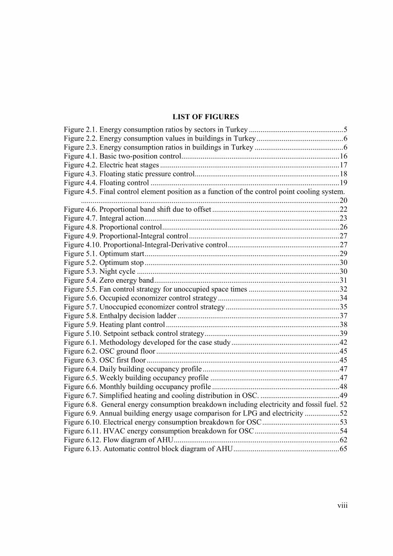
viii

LIST OF FIGURES Figure 2.1. Energy consumption ratios by sectors in Turkey .................................................5 Figure 2.2. Energy consumption values in buildings in Turkey.............................................6 Figure 2.3. Energy consumption ratios in buildings in Turkey ..............................................6 Figure 4.1. Basic two-position control..................................................................................16 Figure 4.2. Electric heat stages .............................................................................................17 Figure 4.3. Floating static pressure control...........................................................................18 Figure 4.4. Floating control ..................................................................................................19 Figure 4.5. Final control element position as a function of the control point cooling system.

......................................................................................................................................20 Figure 4.6. Proportional band shift due to offset ..................................................................22 Figure 4.7. Integral action.....................................................................................................23 Figure 4.8. Proportional control............................................................................................26 Figure 4.9. Proportional-Integral control ..............................................................................27 Figure 4.10. Proportional-Integral-Derivative control..........................................................27 Figure 5.1. Optimum start.....................................................................................................29 Figure 5.2. Optimum stop .....................................................................................................30 Figure 5.3. Night cycle .........................................................................................................30 Figure 5.4. Zero energy band................................................................................................31 Figure 5.5. Fan control strategy for unoccupied space times ...............................................32 Figure 5.6. Occupied economizer control strategy ...............................................................34 Figure 5.7. Unoccupied economizer control strategy ...........................................................35 Figure 5.8. Enthalpy decision ladder ....................................................................................37 Figure 5.9. Heating plant control ..........................................................................................38 Figure 5.10. Setpoint setback control strategy......................................................................39 Figure 6.1. Methodology developed for the case study........................................................42 Figure 6.2. OSC ground floor ...............................................................................................45 Figure 6.3. OSC first floor ....................................................................................................45 Figure 6.4. Daily building occupancy profile .......................................................................47 Figure 6.5. Weekly building occupancy profile ...................................................................47 Figure 6.6. Monthly building occupancy profile ..................................................................48 Figure 6.7. Simplified heating and cooling distribution in OSC. .........................................49 Figure 6.8. General energy consumption breakdown including electricity and fossil fuel. 52 Figure 6.9. Annual building energy usage comparison for LPG and electricity ..................52 Figure 6.10. Electrical energy consumption breakdown for OSC........................................53 Figure 6.11. HVAC energy consumption breakdown for OSC............................................54 Figure 6.12. Flow diagram of AHU......................................................................................62 Figure 6.13. Automatic control block diagram of AHU.......................................................65

ix

LIST OF TABLES Table 6.1. Building occupancy schedule ..............................................................................46 Table 6.2. BMS equipment list .............................................................................................51 Table 6.3. Performance assessment for fossil fuels and electricity in supermarkets[21]. ....55 Table 6.4. CO2 Performance Index Calculation [21]............................................................56 Table 6.5. Cost Performance Index Calculation [21]. ..........................................................57 Table 6.6. CO2 Performance Assessment for Buildings with Fossil Fuel an .......................57 Table 6.7. Cost Performance Assessment for Buildings with Fossil Fuel an.......................57 Table 6.8. Exposure Factor [21]. ..........................................................................................58 Table 6.9. Normalized Performance Indices Calculation [21]. ............................................60 Table 6.10. Power consumptions of AHUs ..........................................................................61 Table 7.1. Summary of energy and environmental data for hypermarket AHU in summer case.......................................................................................................................68

1

Chapter 1

INTRODUCTION

1.1 General

For human beings, energy as work and heat has great importance for the

continuation of life. Energy is the key to industrial development leading to the economic

and social well-being of the world population. The growth of the world population, coupled

with rising material standard of living, has escalated energy usage since the turn of this

century [1].

Modern buildings and their HVAC systems are required to be more energy efficient

while adhering to an ever-increasing demand for better indoor air quality and performance.

Economical considerations and environmental issues also need to be taken into account.

Maintaining high standards of indoor comfort is an economically sound goal.

Research shows that indoor comfort and productivity can be linked [2]. These studies

indicate that the economic gain with a small increase in productivity outweighs energy

savings obtained by reducing the indoor comfort levels. A balance between energy

efficiency and indoor comfort must thus be obtained.

The goal of HVAC design in buildings is to provide comfort to the occupants.

Because heating and cooling loads vary with the time of the day and of the year, an HVAC

system must be complemented with a good control scheme to maintain comfort under any

load conditions. Good control will also reduce energy use by keeping the process variables

(temperature, pressure etc.) to their setpoint efficiently

Efficient HVAC control is often the most cost-effective option to improve the energy

efficiency of a building. However, the effect of changing the control strategy (i.e. on indoor

comfort and energy consumption) is usually difficult to predict. The success of

implementing efficient energy management and control is coupled with understanding the

performance of mechanical and control systems.

2

Control is essential feature of almost every engineering system and process. For many

years, control was affected by analog means only. The advent of the microprocessor,

however, made digital control possible, and cost reduction in their manufacture have led to

their wide spread use in a variety of situations. Their adoption for the control of the

building services systems has come to be known as energy management, and the terms

“Energy Management And Control Systems” (EMCS) in North America and “Building

Energy Management Systems” (BEMS) in Europe are used to describe installations of this

nature [1].

BMSs centralize the monitoring, operations, and management of a building to achieve

more efficient operations. BMSs have become an essential part of a modern building that

contributes significant saving potential and function feasibility. However, the actual

achievement of BMS relies on well-developed and commissioned BMS hardware and

software, well-trained BMS users, and system designers of adequate knowledge and

experience on BMS and dynamic performance of HVAC systems [3].

1.2 Present Study

The aim of the present study is to understand HVAC control principles and their

applications, investigating the potential for energy savings and then reducing the energy

consumptions by the help of BMS within a case study. Quite amount of money is invested

to HVAC and its control systems which need to pay back in a short period. In HVAC

automation sector, lack of knowledge brings long pay back times, high energy consumption

and customer dissatisfaction.

In Chapter 1 the importance of efficient HVAC control and comfort in buildings are

focused, then brief information is given about present study and literature survey. In

Chapter 2 energy consumptions in buildings in Turkey is investigated. Then energy

conservation activities and legislative studies in buildings are focused. Chapter 3 gives

general idea on BMSs and its applications. Chapter 4 is theoretical study which aims to

understand the automatic control principles in HVAC systems. Chapter 5 focuses the main

idea of this thesis. This chapter explains the HVAC control principles and their

applications. In Chapter 6 a case study which was carried out in OSC to investigate the

3

potential for energy savings and to redefine HVAC control strategies are described. A

methodology is developed for systematic approach to the case study. An energy audit is

conducted and consequences are discussed. Performance Indices and Normalized

Performance Indices of the building are determined and compared with accepted standards.

An action plan is defined to initiate a site study. Within the site study current control

scenarios are investigated then redefined strategies are implemented. Finally parameters are

tuned to reduce fluctuations from set points. In Chapter 7 results of the case study are

analyzed and discussed. In Chapter 8 conclusion is made with the overview of the entire

study.

1.3 Literature Survey

Buildings form an important part of the modern lifestyle. Not surprisingly, it is also

one of the largest industry sectors worldwide. Buildings, especially commercial buildings,

are further one of the biggest consumers of energy. In developed countries, buildings

account for between 30% and 40% of the energy consumed. Another alarming fact is that

their energy consumption seems to be on the rise [4]. A report of the American Council for

an Energy Efficient Economy showed that commercial buildings had the highest growth in

energy consumption during the mid 1980s [5].

In general, most of the energy is used to maintain acceptable comfort levels within

buildings. Of this, lighting and HVAC systems form the largest consumption items. Studies

indicate that air-conditioning is responsible for between 10% and 60% of the total building

energy consumption, depending on the building type [6,7].

Mathews et al. (2002) [8] conducted a case study on a Conference Center to increase

its energy efficiency, by optimizing the HVAC system control, and in particular, the control

of the heating plant. They emphasized that approximately 50% of the energy used by the

commercial sector in South Africa is utilized for air-conditioning. This clearly shows that

the HVAC system of a building has a large potential for energy saving. A cost-effective

way to improve the energy efficiency of fan HVAC system, without compromising indoor

comfort, is by implementing better control.

4

Zaheer-uddin et al. [9] explored the problem of computing optimal control strategies

for time-scheduled operation of HVAC systems. The optimization problem that takes into

consideration the building operation schedules consisting of night-setback, start-up,

occupied modes and energy price discounts is formulated and solved for a given predicted

weather profile. Results showing the optimal mass flow rates to the zones, air and water

supply temperatures, energy input to the heat pump and the resulting zone temperatures are

given.

Also some studies have been done on the optimization of supervisory control [10,11].

House et al. [10] investigated the problem of optimal control of the HVAC and building by

using a systems approach.

Shengwei Wang et al. [3] developed dynamic and real-time simulation models to

simulate the thermal, hydraulic, mechanical, environmental and energy performance of

building a variable air volume VAV air-conditioning system and its BMS. A window-based

user’s interface is developed to simulate the man–machine interface of a BMS, through

which users can monitor the on-line operation, tune the local control loops, and reset the

supervisory control strategies.

Mathews et al. (2002) [12] developed a simulation tool, QUICK control to predict

effect of changing control strategies (i.e. on indoor comfort and energy consumption) more

easily. This tool was then used to investigate the energy savings potential in a Conference

Center. The influences of fan scheduling, setpoint setback, economizer cycle, new

setpoints, fan control, heating plant control, lighting control and various combinations

thereof was investigated. The simulation models were firstly verified with measurements

obtained from the existing system to confirm their accuracy for realistic control retrofit

simulations. With the aid of the integrated simulation tool it was possible to predict savings

of 744 MWh per year (32% building energy saving and 58% HVAC system energy saving)

by implementing these control strategies. These control strategies can be implemented in

the building with a direct payback period of less than 6 months.

5

Chapter 2

ENERGY CONSUMPTIONS AND ENERGY CONSERVATION ACTIVITIES IN BUILDINGS IN TURKEY

2.1 Overview

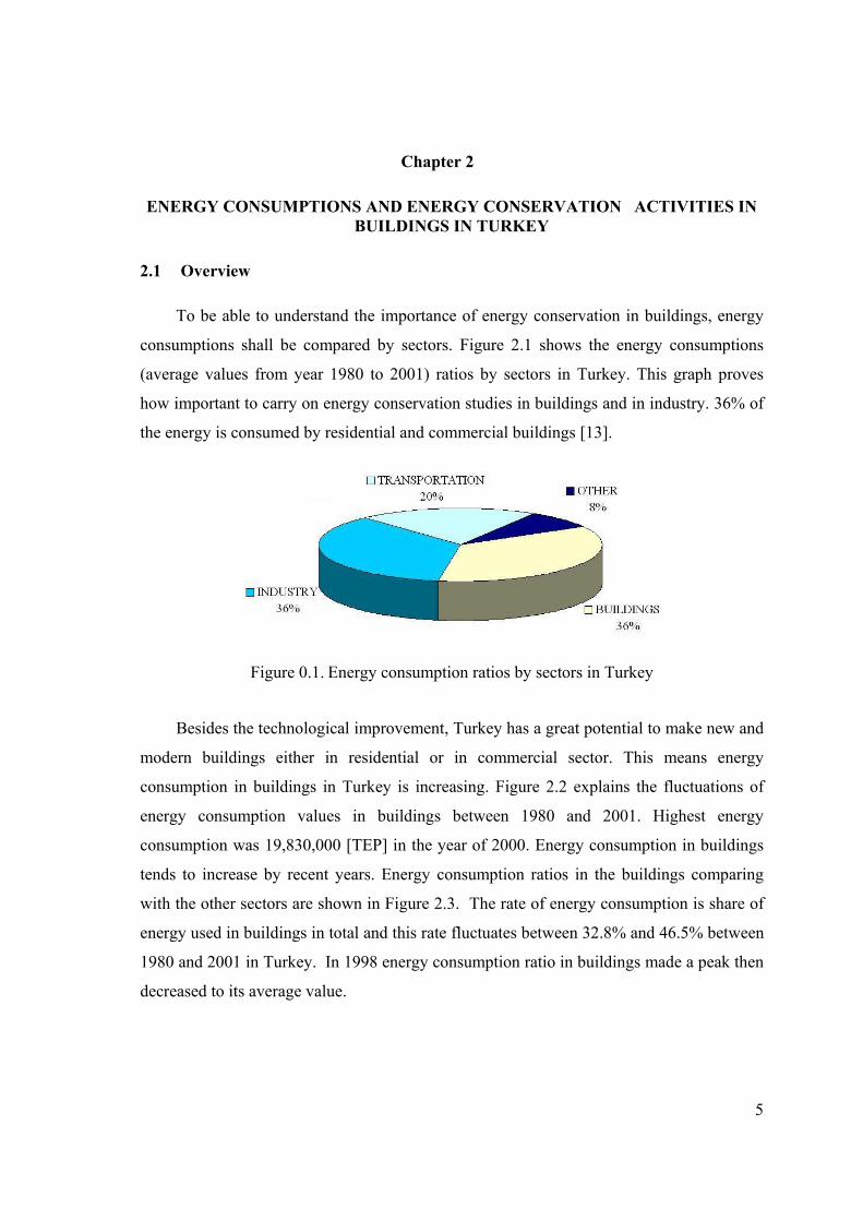
To be able to understand the importance of energy conservation in buildings, energy

consumptions shall be compared by sectors. Figure 2.1 shows the energy consumptions

(average values from year 1980 to 2001) ratios by sectors in Turkey. This graph proves

how important to carry on energy conservation studies in buildings and in industry. 36% of

the energy is consumed by residential and commercial buildings [13].

Figure 0.1. Energy consumption ratios by sectors in Turkey

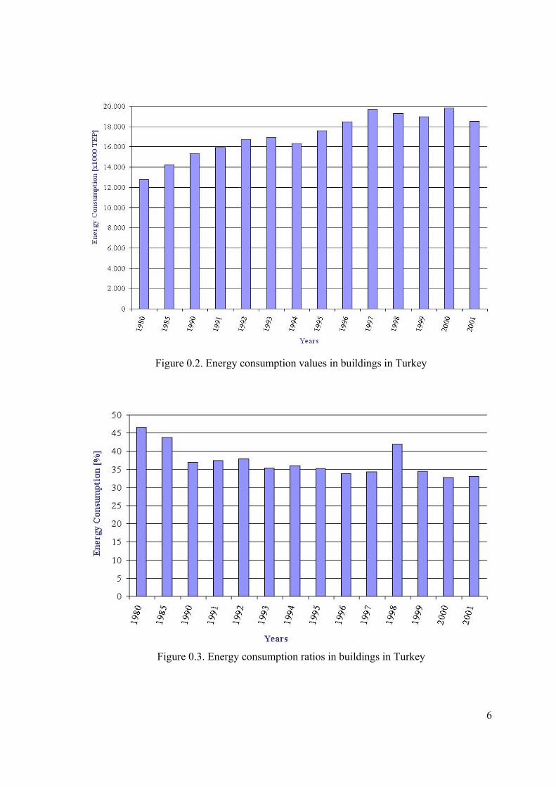
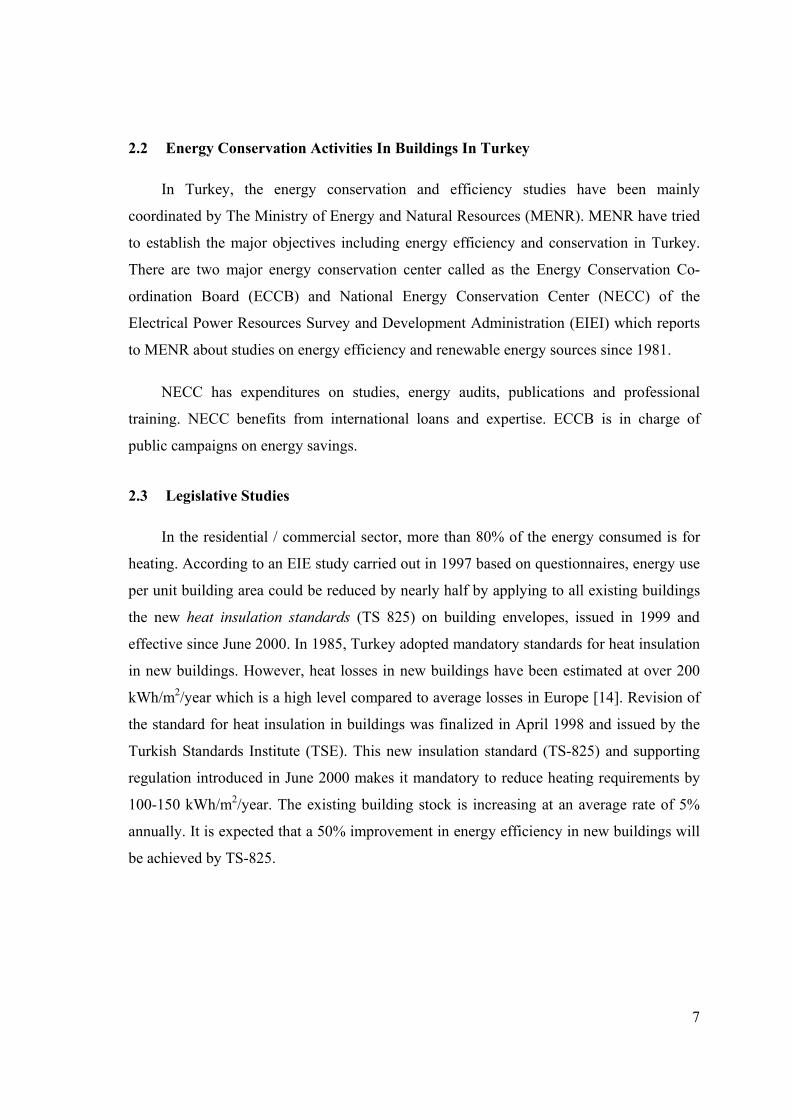
Besides the technological improvement, Turkey has a great potential to make new and

modern buildings either in residential or in commercial sector. This means energy

consumption in buildings in Turkey is increasing. Figure 2.2 explains the fluctuations of

energy consumption values in buildings between 1980 and 2001. Highest energy

consumption was 19,830,000 [TEP] in the year of 2000. Energy consumption in buildings

tends to increase by recent years. Energy consumption ratios in the buildings comparing

with the other sectors are shown in Figure 2.3. The rate of energy consumption is share of

energy used in buildings in total and this rate fluctuates between 32.8% and 46.5% between

1980 and 2001 in Turkey. In 1998 energy consumption ratio in buildings made a peak then

decreased to its average value.

6

Figure 0.2. Energy consumption values in buildings in Turkey

Figure 0.3. Energy consumption ratios in buildings in Turkey

7

2.2 Energy Conservation Activities In Buildings In Turkey

In Turkey, the energy conservation and efficiency studies have been mainly

coordinated by The Ministry of Energy and Natural Resources (MENR). MENR have tried

to establish the major objectives including energy efficiency and conservation in Turkey.

There are two major energy conservation center called as the Energy Conservation Co-

ordination Board (ECCB) and National Energy Conservation Center (NECC) of the

Electrical Power Resources Survey and Development Administration (EIEI) which reports

to MENR about studies on energy efficiency and renewable energy sources since 1981.

NECC has expenditures on studies, energy audits, publications and professional

training. NECC benefits from international loans and expertise. ECCB is in charge of

public campaigns on energy savings.

2.3 Legislative Studies

In the residential / commercial sector, more than 80% of the energy consumed is for

heating. According to an EIE study carried out in 1997 based on questionnaires, energy use

per unit building area could be reduced by nearly half by applying to all existing buildings

the new heat insulation standards (TS 825) on building envelopes, issued in 1999 and

effective since June 2000. In 1985, Turkey adopted mandatory standards for heat insulation

in new buildings. However, heat losses in new buildings have been estimated at over 200

kWh/m2/year which is a high level compared to average losses in Europe [14]. Revision of

the standard for heat insulation in buildings was finalized in April 1998 and issued by the

Turkish Standards Institute (TSE). This new insulation standard (TS-825) and supporting

regulation introduced in June 2000 makes it mandatory to reduce heating requirements by

100-150 kWh/m2/year. The existing building stock is increasing at an average rate of 5%

annually. It is expected that a 50% improvement in energy efficiency in new buildings will

be achieved by TS-825.

8

2.4 Governmental Buildings Energy Conservation Monitoring Programme

In accordance with the circular entitled measures to be taken by Governmental

Organizations and Institutions in order to reduce their energy consumption issued by the

Prime Minister, all governmental organizations have prepared annual reports on energy

consumption in their buildings. These reports were sent to EIE/NECC by the ministry and

evaluated by ECC. In 1999, information concerning 2,037 governmental buildings was

evaluated [15]. According to the evaluation results, the energy consumption of these

buildings was very high (more than 250 kWh/m2/year); only 48% of them have double-

glazing and 40% have roof insulation.

Another project named “Application of Energy Efficiency Studies in Buildings in

Erzurum” has been initiated in co-operation with the German technical organization (GTZ),

the Erzurum Municipality and EIE/NECC in November, 2002. The duration of this project

will be three years. Its aim is to enable municipal authorities as well as users of public and

private buildings to take measures designed to reduce the use of energy in buildings.

Implementation of the project will be realized in Erzurum and studies related to standards,

regulations and training will be carried out in Ankara.

2.5 Statistical Studies

At the end of 1997, in co-operation with the State Institute of Statistics (SIS), a

statistical study for the analysis of energy consumption of residential buildings, which

covered the whole country, was launched. In this project, the analysis of the energy

consumption in terms of fuel and electricity, the insulation status, heating systems, and the

structural properties of the residential buildings have been realized on the basis of

geographical regions.

2.6 Energy Labeling / Standards

Under the co-ordination and supervision of EIE/NECC, and with the participation of

representatives of the related manufacturers and public organizations, working groups have

been set up on energy efficiency of household appliances, air conditioners and lightning.

9

The related analytic work reveals that new regulations are needed to increase energy

efficiency for the before-mentioned equipment. In this context, studies to prepare energy

efficiency labeling standards and regulations for electrical appliances have already been

initiated by the TSE and the Ministry of Industry and Trade (MIT) within the framework of

the Harmonization Programme for EU legislation. regulation on energy efficiency labeling

for refrigerators was issued on March 2002. The other labeling regulations related to

washing machines, dryers, dish washers and lamps have been prepared and should soon be

published by the MIT. The energy efficiency regulation for outdoor (street) lighting is

under review. In the 2000/2001 in-depth reviews of the energy policies of Turkey, the IEA

stated: The Government of Turkey should enhance Turkey's participation in international

co-operation programmes on energy efficiency, in particular on efficiency standards and

labels for household appliances and motor vehicles and should consider establishing fiscal

and economic incentives for conservation measures in all sectors.

10

Chapter 3

BUILDING MANAGEMENT SYSTEMS (BMSs)

3.1 Introduction

The objective of BMSs is to centralize and simplify the monitoring, operation, and

management of a building or buildings. This is done to achieve more efficient building

operation at reduced labor and energy costs and provide a safe and more comfortable

working environment for building occupants. In the process of meeting these objectives,

the BMS has evolved from simple supervisory control to totally integrated computerized

control. Some of the advantages of BMSs are as follows:

1. Simpler operation with routine and repetitive functions programmed for automatic

operation.

2. Reduced operator training time through on-screen instructions and supporting graphic

displays.

3. Faster and better responsiveness to occupant needs and trouble conditions.

4. Reduced energy cost through centralized management of control and energy

management programs.

5. Better management of the facility through historical records, maintenance

management programs, and automatic alarm reporting.

6. Flexibility of programming for facility needs, size, organization, and expansion

requirements.

7. Improved operating-cost record keeping for allocating to cost centers and/or charging

individual occupants.

8. Improved operation through software and hardware integration of multiple

subsystems such as direct digital control (DDC), fire alarm, security, access control,

or lighting control.

When minicomputers and mainframes were the only computers available, the BMS

was only used on larger office buildings and college campuses. With the shift to

microprocessor-based controllers for DDC, the cost of integrating BMS functions into the

11

controller is so small that a BMS is a good investment for commercial buildings of all types

and sizes.

Some other benefits of BMSs shall be expressed as follows: [16]

A. MONITORING: Constant monitoring of the plant, and ability to recall the monitored

data at a later time. This has enables engineers and technicians to achieve a better

understanding of their buildings and plant and has often led to plant improvements

and energy saving as a result. Energy efficiency can be checked as a BMS can

monitor and log data from fuel & electricity meters.

B. COMMUNICATION: Developments on personal computers and internet technology

led BMS to communicate from anywhere. By web server function operator can reach

to site from anywhere in the world.

C. MANPOWER SAVINGS & MAINTENANCE: The local boilerman, caretaker or plant

operator can often be replaced by communicating BMS outstation, or one operator

can cover more buildings. Especially maintenance contractors and energy

management bureaus offer to run clients’ buildings and plant for them using

outstations communicating regularly with the central station at the organizations

headquarters.

D. COMMISSIONING: BMSs are becoming used in aiding the commissioning of plant

in newly constructed buildings. This is rather used in large air conditioned office

blocks with many small outstations on the air conditioning units around the building.

Some problems with BMSs shall be expressed as follows:

1. Associated with computers.

2. Large user manuals to explain many functions and operations that they can perform.

User manuals are also not user friendly.

3. Training courses are expensive.

4. Software has continuously new versions to adapt.

12

5. The manipulation of energy data for monitoring and targeting the buildings is also a

problem. A survey in 1990[17, 16] of 50 energy managers showed that 82% had BMS

but only 2% could use them for targeting.

6. Clearly, BMSs are not being used to their full potential.

7. Incompatible devices and protocols from different manufacturers and problems to

communicate the devices.

3.2 Background

The BMS concept emerged in the early 1950s and has since changed dramatically

both in scope and system configuration. System communications evolved from hardwired

(and homerun piping for pneumatic centralization) to multiplexed (shared wiring) to

today’s two-wire all digital system. The Energy Management System (EMS) and BMCS

evolved from poll-response protocols with central control processors to peer-to-peer

protocols with distributed control.

3.3 Energy Management

Energy management is typically a function of the microprocessor-based Direct Digital

Controller (DDC). In most mid-sized to large buildings, energy management is an integral

part of the BMCS, with optimized control performed at the system level and with

management information and user access provided by the BMS host. Equipment is operated

at a minimum cost and temperatures are controlled for maximum efficiency within user-

defined comfort boundaries by a network of controllers. Energy strategies are global and

network communications are essential.

Load leveling and demand control along with starting and loading of central plant

based upon the demands of air handling systems require continuous global system

coordination [18]. Energy Management BMS host functions include the followings:

1. Efficiency monitoring and recording.

2. Energy usage monitoring and recording.

3. Energy summaries.

13

a. Energy usage by source and by time period.

b. On-times, temperatures, efficiencies by system, building, area.

4. Curve plots of trends.

5. Access to energy management strategies for continuous tuning and adapting to

changing needs.

a. Occupancy schedules.

b. Comfort limit temperatures.

c. Parametric adjustments (e.g., integral gain) of DDC loops.

d. Setpoint adjustments.

i. Duct static pressures.

ii. Economizer changeover values.

iii. Water temperatures and schedules.

6. Modifying and adding DDC programs Energy Management for buildings preceded

DDC by about ten years.

These pre-DDC systems were usually a digital architecture consisting of a central

computer which contained the monitoring and control strategies and remote Data Gathering

Panels (DGPs) which interfaced with local pneumatic, electric, and electronic control

systems. The central computer issued optimized start/stop commands and adjusted local

loop temperature controllers.

3.4 Facilities Management Systems

Facilities management, introduced in the late 1980s, broadened the scope of central

control to include the management of a total facility. In an automotive manufacturing plant,

for example, production scheduling and monitoring can be included with normal BMS

environmental control and monitoring. The production and BMS personnel can have

separate distributed systems for control of inputs and outputs, but the systems are able to

exchange data to generate management reports. For example, a per-car cost allocation for

heating, ventilating, and air conditioning overhead might be necessary management

information for final pricing of the product.

14

Facilities management system configuration must deal with two levels of operation:

day-to-day operations and long-range management and planning. Day-to-day operations

require a real-time system for constant monitoring and control of the environment and

facility. The management and planning level requires data and reports that show long-range

trends and progress against operational goals. Therefore, the primary objective of the

management and planning level is to collect historical data, process it, and present the data

in a usable format. The development of two-wire transmission systems, PCs for centralized

functions, and distributed processors including DDC led to a need to define system

configurations. These configurations became based on the needs of the building and the

requirements of the management and operating personnel.

1. System functions general.

2. Zone-level controller functions.

3. System-level controller functions.

4. Operations-level functions general.

a. Hardware.

b. Software.

i. Standard Software.

ii. Communications Software.

iii. Server.

iv. Security.

v. Alarm Processing.

vi. Reports.

vii. System Text.

viii. System Graphics.

ix. Controller Support.

15

Chapter 4

BASIS OF AUTOMATIC CONTROL-THEORETICAL STUDY

4.1 Introduction

Automatic controls are used wherever a variable condition must be controlled. In

HVAC systems, the most commonly controlled conditions are pressure, temperature,

humidity, and rate of flow. Applications of automatic control systems range from simple

residential temperature regulation to precision control of industrial processes [19].

4.2 Control Modes

Control systems use different control modes to accomplish their purposes. Control

modes in commercial applications include two-position, step, and floating control;

proportional, proportional-integral, and proportional – integral - derivative control; and

adaptive control.

4.2.1 Two-Position Control

In two-position control, the final control element occupies one of two possible

positions except for the brief period when it is passing from one position to the other. Two-

position control is used in simple HVAC systems to start and stop electric motors on unit

heaters, fan coil units, and refrigeration machines, to open water sprays for humidification,

and to energize and de-energize electric strip heaters. Basic two-position control works well

for many applications. For close temperature control, however, the cycling must be

accelerated or timed.

4.2.1.1 Basic Two-Position Control

In basic two-position control, the controller and the final control element interact

without modification from a mechanical or thermal source. The result is cyclical operation

of the controlled equipment and a condition in which the controlled variable cycles back

and forth between two values (the on and off points) and is influenced by the lag in the

system (Figure 4.1). The controller cannot change the position of the final control element

16

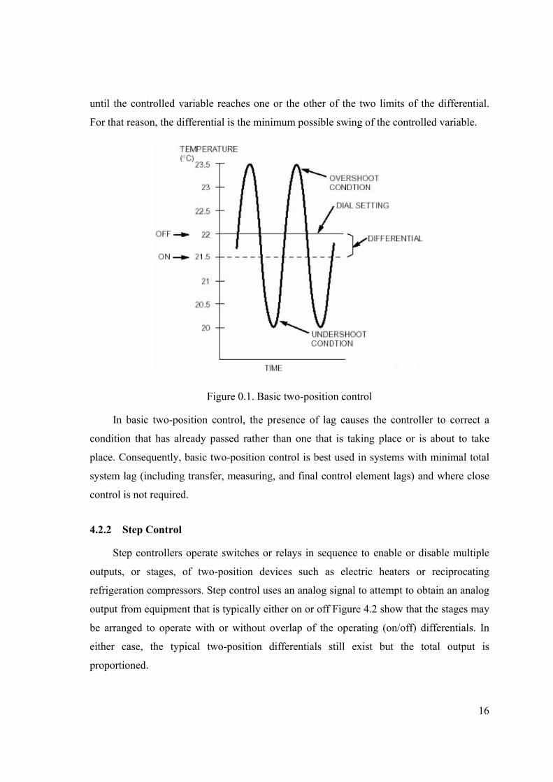
until the controlled variable reaches one or the other of the two limits of the differential.

For that reason, the differential is the minimum possible swing of the controlled variable.

Figure 0.1. Basic two-position control

In basic two-position control, the presence of lag causes the controller to correct a

condition that has already passed rather than one that is taking place or is about to take

place. Consequently, basic two-position control is best used in systems with minimal total

system lag (including transfer, measuring, and final control element lags) and where close

control is not required.

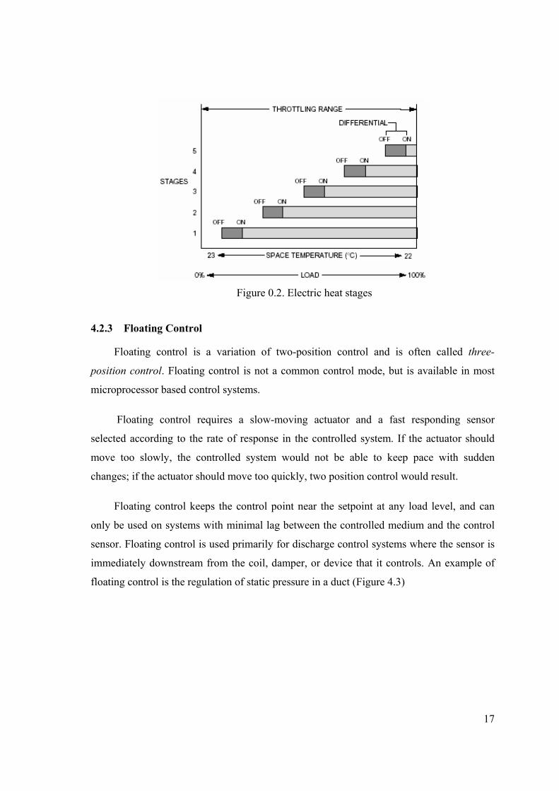
4.2.2 Step Control

Step controllers operate switches or relays in sequence to enable or disable multiple

outputs, or stages, of two-position devices such as electric heaters or reciprocating

refrigeration compressors. Step control uses an analog signal to attempt to obtain an analog

output from equipment that is typically either on or off Figure 4.2 show that the stages may

be arranged to operate with or without overlap of the operating (on/off) differentials. In

either case, the typical two-position differentials still exist but the total output is

proportioned.

17

Figure 0.2. Electric heat stages

4.2.3 Floating Control

Floating control is a variation of two-position control and is often called three-

position control. Floating control is not a common control mode, but is available in most

microprocessor based control systems.

Floating control requires a slow-moving actuator and a fast responding sensor

selected according to the rate of response in the controlled system. If the actuator should

move too slowly, the controlled system would not be able to keep pace with sudden

changes; if the actuator should move too quickly, two position control would result.

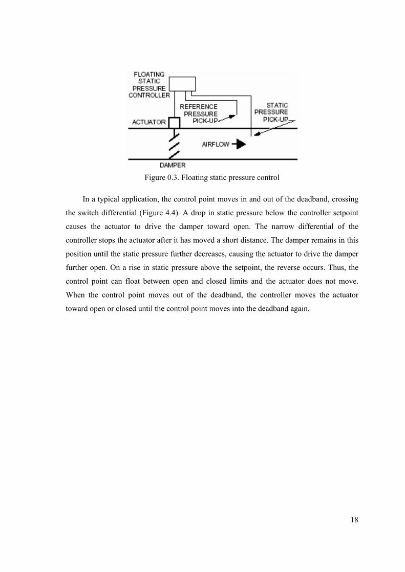
Floating control keeps the control point near the setpoint at any load level, and can

only be used on systems with minimal lag between the controlled medium and the control

sensor. Floating control is used primarily for discharge control systems where the sensor is

immediately downstream from the coil, damper, or device that it controls. An example of

floating control is the regulation of static pressure in a duct (Figure 4.3)

18

Figure 0.3. Floating static pressure control

In a typical application, the control point moves in and out of the deadband, crossing

the switch differential (Figure 4.4). A drop in static pressure below the controller setpoint

causes the actuator to drive the damper toward open. The narrow differential of the

controller stops the actuator after it has moved a short distance. The damper remains in this

position until the static pressure further decreases, causing the actuator to drive the damper

further open. On a rise in static pressure above the setpoint, the reverse occurs. Thus, the

control point can float between open and closed limits and the actuator does not move.

When the control point moves out of the deadband, the controller moves the actuator

toward open or closed until the control point moves into the deadband again.

19

Figure 0.4. Floating control

4.2.4 Proportional Control

Proportional control proportions the output capacity of the equipment (e.g., the

percent a valve is open or closed) to match the heating or cooling load on the building,

unlike two-position control in which the mechanical equipment is either full on or full off.

In this way, proportional control achieves the desired heat replacement or displacement

rate.

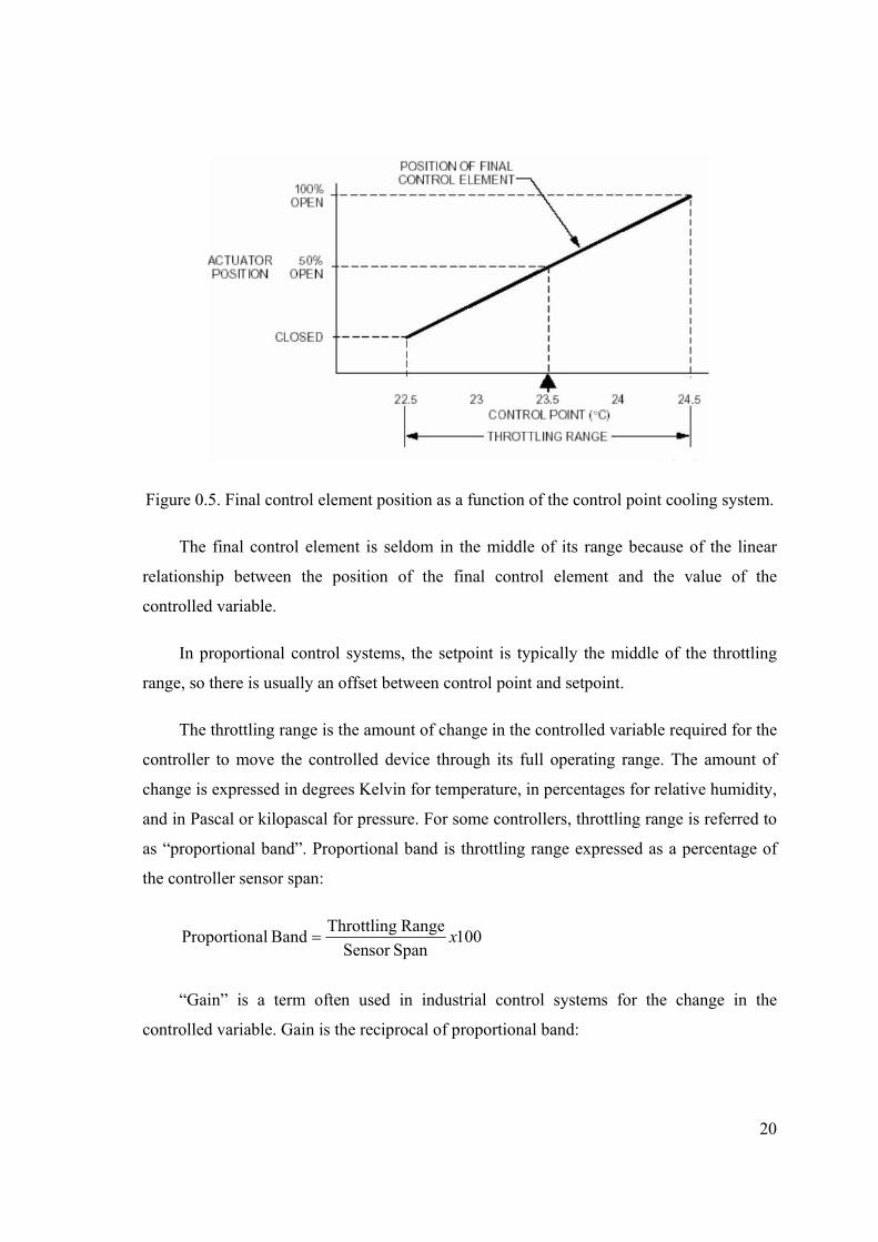
In proportional control, the final control element moves to a position proportional to

the deviation of the value of the controlled variable from the setpoint. The position of the

final control element is a linear function of the value of the controlled variable (Figure 4.5)

20

Figure 0.5. Final control element position as a function of the control point cooling system.

The final control element is seldom in the middle of its range because of the linear

relationship between the position of the final control element and the value of the

controlled variable.

In proportional control systems, the setpoint is typically the middle of the throttling

range, so there is usually an offset between control point and setpoint.

The throttling range is the amount of change in the controlled variable required for the

controller to move the controlled device through its full operating range. The amount of

change is expressed in degrees Kelvin for temperature, in percentages for relative humidity,

and in Pascal or kilopascal for pressure. For some controllers, throttling range is referred to

as “proportional band”. Proportional band is throttling range expressed as a percentage of

the controller sensor span:

100SpanSensor Range ThrottlingBand alProportion x=

“Gain” is a term often used in industrial control systems for the change in the

controlled variable. Gain is the reciprocal of proportional band:

21

Band alProportion100

=Gain

The output of the controller is proportional to the deviation of the control point from

setpoint. A proportional controller can be mathematically described by:

V = KE + M

Where:

V = output signal K = proportionality constant (gain) E = deviation (control point - setpoint) M = value of the output when the deviation is zero

(Usually the output value at 50 percent or the middle of the output range. The

generated control signal correction is added to or subtracted from this value. Also called

“bias” or “manual reset”.)

4.2.5 Proportional-Integral (PI) Control

In the proportional-integral (PI) control mode, reset of the control point is automatic.

PI control, also called “proportional plus - reset” control, virtually eliminates offset and

makes the proportional band nearly invisible. As soon as the controlled variable deviates

above or below the setpoint and offset develops, the proportional band gradually and

automatically shifts, and the variable is brought back to the setpoint. The major difference

between proportional and PI control is that proportional control is limited to a single final

control element position for each value of the controlled variable. PI control changes the

final control element position to accommodate load changes while keeping the control

point at or very near the setpoint.

The reset action of the integral component shifts the proportional band as necessary

around the setpoint as the load on the system changes. The graph in Figure 4.6 shows the

shift of the proportional band of a PI controller controlling a normally open heating valve.

The shifting of the proportional band keeps the control point at setpoint by making further

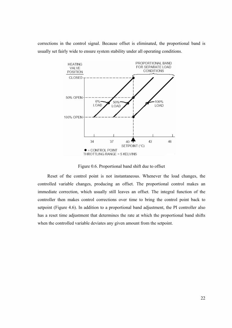
22

corrections in the control signal. Because offset is eliminated, the proportional band is

usually set fairly wide to ensure system stability under all operating conditions.

Figure 0.6. Proportional band shift due to offset

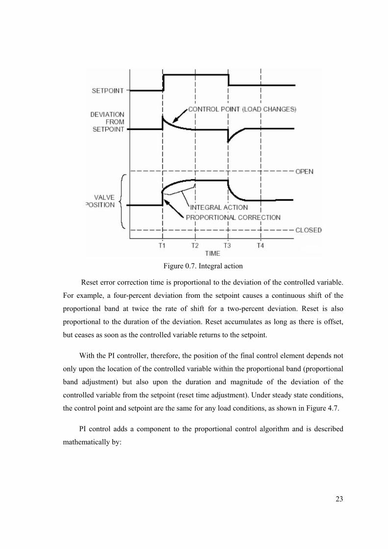
Reset of the control point is not instantaneous. Whenever the load changes, the

controlled variable changes, producing an offset. The proportional control makes an

immediate correction, which usually still leaves an offset. The integral function of the

controller then makes control corrections over time to bring the control point back to

setpoint (Figure 4.6). In addition to a proportional band adjustment, the PI controller also

has a reset time adjustment that determines the rate at which the proportional band shifts

when the controlled variable deviates any given amount from the setpoint.

23

Figure 0.7. Integral action

Reset error correction time is proportional to the deviation of the controlled variable.

For example, a four-percent deviation from the setpoint causes a continuous shift of the

proportional band at twice the rate of shift for a two-percent deviation. Reset is also

proportional to the duration of the deviation. Reset accumulates as long as there is offset,

but ceases as soon as the controlled variable returns to the setpoint.

With the PI controller, therefore, the position of the final control element depends not

only upon the location of the controlled variable within the proportional band (proportional

band adjustment) but also upon the duration and magnitude of the deviation of the

controlled variable from the setpoint (reset time adjustment). Under steady state conditions,

the control point and setpoint are the same for any load conditions, as shown in Figure 4.7.

PI control adds a component to the proportional control algorithm and is described

mathematically by:

24

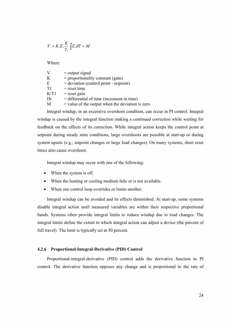
MdTETKEKV += ∫ ...

1

Where:

V = output signal K = proportionality constant (gain) E = deviation (control point - setpoint) T1 = reset time K/T1 = reset gain Dt = differential of time (increment in time) M = value of the output when the deviation is zero

Integral windup, or an excessive overshoot condition, can occur in PI control. Integral

windup is caused by the integral function making a continued correction while waiting for

feedback on the effects of its correction. While integral action keeps the control point at

setpoint during steady state conditions, large overshoots are possible at start-up or during

system upsets (e.g., setpoint changes or large load changes). On many systems, short reset

times also cause overshoot.

Integral windup may occur with one of the following:

• When the system is off.

• When the heating or cooling medium fails or is not available.

• When one control loop overrides or limits another.

Integral windup can be avoided and its effects diminished. At start-up, some systems

disable integral action until measured variables are within their respective proportional

bands. Systems often provide integral limits to reduce windup due to load changes. The

integral limits define the extent to which integral action can adjust a device (the percent of

full travel). The limit is typically set at 50 percent.

4.2.6 Proportional-Integral-Derivative (PID) Control

Proportional-integral-derivative (PID) control adds the derivative function to PI

control. The derivative function opposes any change and is proportional to the rate of

25

dTdETK D.

change. The more quickly the control point changes, the more corrective action the

derivative function provides.

If the control point moves away from the setpoint, the derivative function outputs a

corrective action to bring the control point back more quickly than through integral action

alone. If the control point moves toward the setpoint, the derivative function reduces the

corrective action to slow down the approach to setpoint, which reduces the possibility of

overshoot.

The rate time setting determines the effect of derivative action. The proper setting

depends on the time constants of the system being controlled. The derivative portion of PID

control is expressed in the following formula. Note that only a change in the magnitude of

the deviation can affect the output signal.

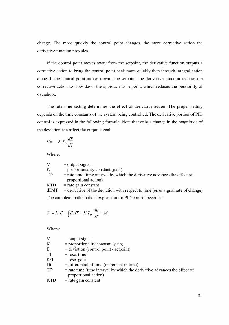
V=

Where:

V = output signal K = proportionality constant (gain) TD = rate time (time interval by which the derivative advances the effect of proportional action) KTD = rate gain constant dE/dT = derivative of the deviation with respect to time (error signal rate of change)

The complete mathematical expression for PID control becomes:

MdTdETKdTEEKV D +++= ∫ ...

Where:

V = output signal K = proportionality constant (gain) E = deviation (control point - setpoint) T1 = reset time K/T1 = reset gain Dt = differential of time (increment in time) TD = rate time (time interval by which the derivative advances the effect of proportional action) KTD = rate gain constant

26

dE/dt = derivative of the deviation with respect to time (error signal rate of change) M = value of the output when the deviation is zero

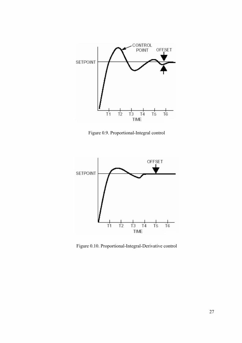
The graphs in Figure 4.8, Figure 4.9 and Figure 4.10 show the effects of all three

modes on the controlled variable at system start-up. With proportional control (Fig. 11), the

output is a function of the deviation of the controlled variable from the setpoint. As the

control point stabilizes, offset occurs. With the addition of integral control (Fig. 12), the

control point returns to setpoint over a period of time with some degree of overshoot. The

significant difference is the elimination of offset after the system has stabilized. Figure 13

shows that adding the derivative element reduces overshoot and decreases response time.

Figure 0.8. Proportional control

27

Figure 0.9. Proportional-Integral control

Figure 0.10. Proportional-Integral-Derivative control

28

Chapter 5

HVAC CONTROL PRINCIPLES FOR ENERGY CONSERVATION

After the general needs of a building have been established, and building and system

subdivision has been made, the mechanical system and its control approach can be

considered. Designing systems that conserve energy requires knowledge of the building, its

operating schedule, the systems to be installed, and ASHRAE Standard 90.1.(A set of

requirements for the energy efficient design of commercial buildings).

Care must be taken while following energy conservation strategies. HVAC systems

are non-linear and characteristics changes on a seasonal basis so implemented strategies

might cause to consume more energy in the following season. Because of that all

implemented strategies shall be checked for seasonal changes. Main HVAC control

principles or approaches that conserve energy are as follows:

5.1 Supplying Heating and Cooling From the Most Efficient Source

Free or low-cost energy sources such as solar and geothermal energy should be used

first, and then higher cost sources as necessary. If electric prices are time-scheduled, high

demand loads should be used in the cheapest time-schedule.

5.2 Running Equipment Only When Needed

HVAC unit operation shall be scheduled for occupied periods. Morning warm-up can

be started as late as possible to achieve design internal temperature by occupancy time,

considering residual space temperature, outdoor temperature, and equipment capacity

(optimum start control). Under most conditions, equipment can be shut down some time

before the end of occupancy, depending on internal and external load and space

temperature (optimum stop control). Shutdown time shall be calculated so that space

temperature does not drift out of the selected comfort zone before the end of occupancy.

Heating shall be started at night only to maintain internal temperature between 10 and 13°C

to prevent freezing.

29

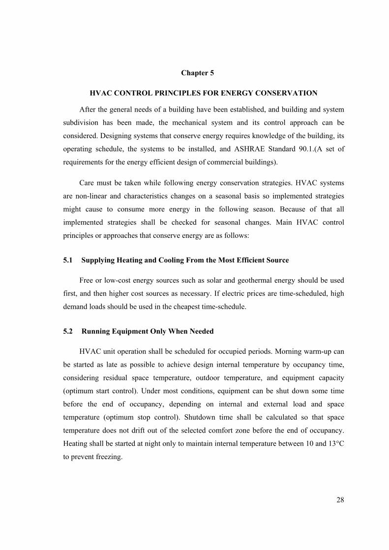
5.2.1 Optimum Start

Based on measurements of indoor and outdoor temperatures and a historical multiplier

adjusted by startup data from the previous day, the optimum start strategy (Figure 5.1)

calculates a lead time to turn on heating or cooling equipment at the optimum time to bring

temperatures to proper level at the time of occupancy. To achieve these results the constant

volume Air Handling Unit (AHU) optimum start program delays AHU start as long as

possible, while the Variable Air Volume (VAV) optimum start program often runs the

VAV AHU at reduced capacity. Unless required by Indoor Air Quality (IAQ), outdoor air

dampers and ventilation fans should be inactive during preoccupancy warm up periods. For

weekend shutdown periods, the program automatically adjusts to provide longer lead times.

This strategy adapts itself to seasonal and building changes.

Figure 0.1. Optimum start

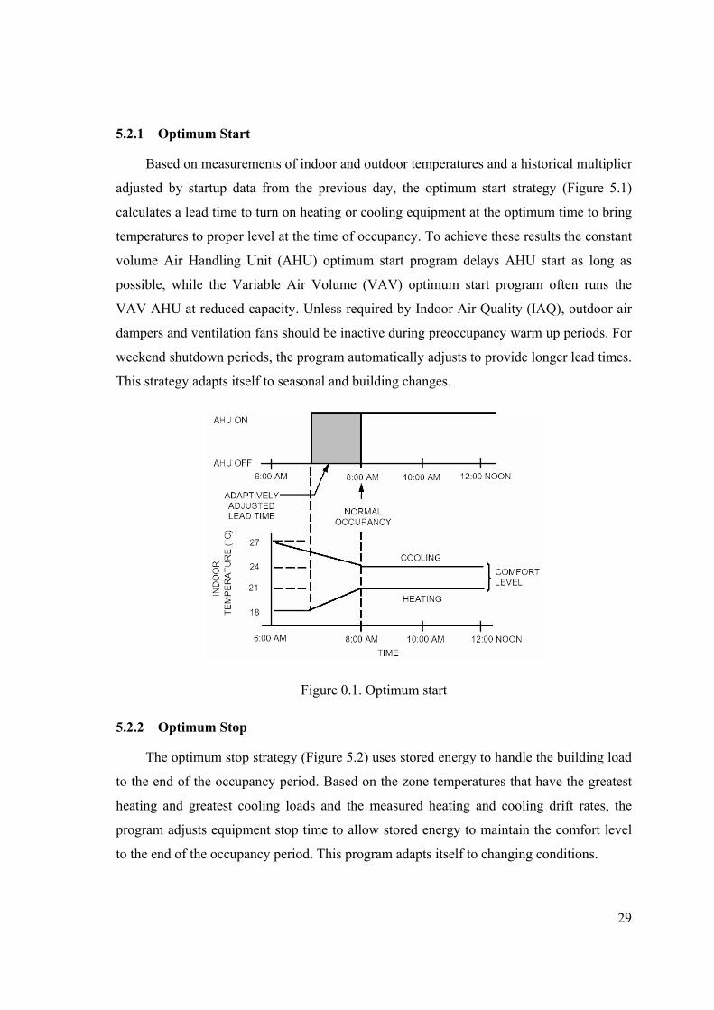
5.2.2 Optimum Stop

The optimum stop strategy (Figure 5.2) uses stored energy to handle the building load

to the end of the occupancy period. Based on the zone temperatures that have the greatest

heating and greatest cooling loads and the measured heating and cooling drift rates, the

program adjusts equipment stop time to allow stored energy to maintain the comfort level

to the end of the occupancy period. This program adapts itself to changing conditions.

30

Figure 0.2. Optimum stop

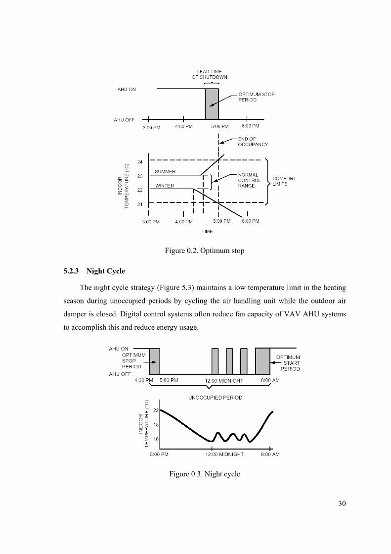
5.2.3 Night Cycle

The night cycle strategy (Figure 5.3) maintains a low temperature limit in the heating

season during unoccupied periods by cycling the air handling unit while the outdoor air

damper is closed. Digital control systems often reduce fan capacity of VAV AHU systems

to accomplish this and reduce energy usage.

Figure 0.3. Night cycle

31

5.3 Sequencing Heating And Cooling

Heating and cooling should not be supplied simultaneously. Central fan systems

should use cool outdoor air in sequence between heating and cooling. Zoning and system

selection should eliminate, or at least minimize, simultaneous heating and cooling. Also,

humidification and dehumidification should not take place concurrently.

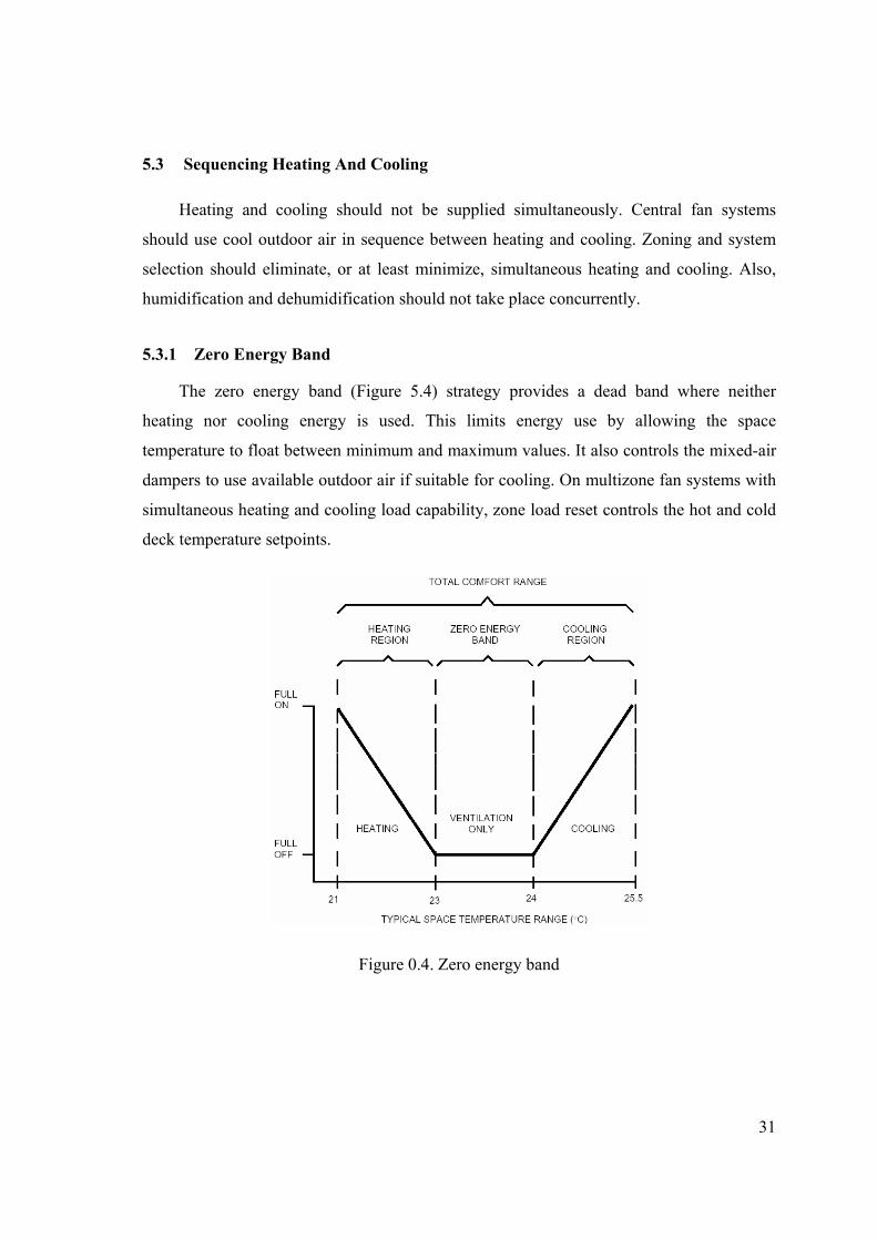
5.3.1 Zero Energy Band

The zero energy band (Figure 5.4) strategy provides a dead band where neither

heating nor cooling energy is used. This limits energy use by allowing the space

temperature to float between minimum and maximum values. It also controls the mixed-air

dampers to use available outdoor air if suitable for cooling. On multizone fan systems with

simultaneous heating and cooling load capability, zone load reset controls the hot and cold

deck temperature setpoints.

Figure 0.4. Zero energy band

32

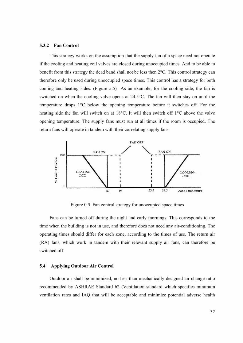
5.3.2 Fan Control

This strategy works on the assumption that the supply fan of a space need not operate

if the cooling and heating coil valves are closed during unoccupied times. And to be able to

benefit from this strategy the dead band shall not be less then 2°C. This control strategy can

therefore only be used during unoccupied space times. This control has a strategy for both

cooling and heating sides. (Figure 5.5) As an example; for the cooling side, the fan is

switched on when the cooling valve opens at 24.5°C. The fan will then stay on until the

temperature drops 1°C below the opening temperature before it switches off. For the

heating side the fan will switch on at 18°C. It will then switch off 1°C above the valve

opening temperature. The supply fans must run at all times if the room is occupied. The

return fans will operate in tandem with their correlating supply fans.

Figure 0.5. Fan control strategy for unoccupied space times

Fans can be turned off during the night and early mornings. This corresponds to the

time when the building is not in use, and therefore does not need any air-conditioning. The

operating times should differ for each zone, according to the times of use. The return air

(RA) fans, which work in tandem with their relevant supply air fans, can therefore be

switched off.

5.4 Applying Outdoor Air Control

Outdoor air shall be minimized, no less than mechanically designed air change ratio

recommended by ASHRAE Standard 62 (Ventilation standard which specifies minimum

ventilation rates and IAQ that will be acceptable and minimize potential adverse health

33

effects.) should be used. In areas where it is cost-effective, enthalpy should be used rather

than dry-bulb temperature to determine whether outdoor or RA is the most energy-efficient

air source for the cooling mode.

For heating plant, setpoint shifting should be implemented due to outdoor air

temperature. This strategy is called outdoor air compensation.

5.4.1 Outdoor Air Dry Bulb Temperature Control

Outdoor air is used for cooling anytime the OA temperature is below the setpoint. For

successful operation, local weather data analysis needed to determine the optimum

changeover setpoint. The analysis need only consider data when the OA is between

approximately 16°C and 25.5°C, and during the occupancy period. The dry bulb

economizer decision is best on small systems (where the cost of a good humidity sensor

cannot be justified), where maintenance cannot be relied upon, or where there are not

frequent wide variations in OA RH during the decision window (when the OA is between

approximately 16°C and 25.5°C).

The minimum set for outdoor air damper shall not be considered if the space is not

occupied. So this strategy can be divided into two parts, an occupied strategy and an

unoccupied strategy. Infrared motion detectors should be located in the space which will be

responsible for selecting the relevant strategy. The occupied strategy will be active for 15

min after movement was detected by any of the sensors in the space. This implies that the

timer will reset itself if new movement is detected during this period and the 15-min

countdown will start all over again. The unoccupied strategy will therefore only be

activated when all the sensors in the space are passive for a period of 15 min. For this

option all the relevant motion detectors of the space which RA to the same set of dampers

must be passive for 15 min to activate the unoccupied economizer control strategy.

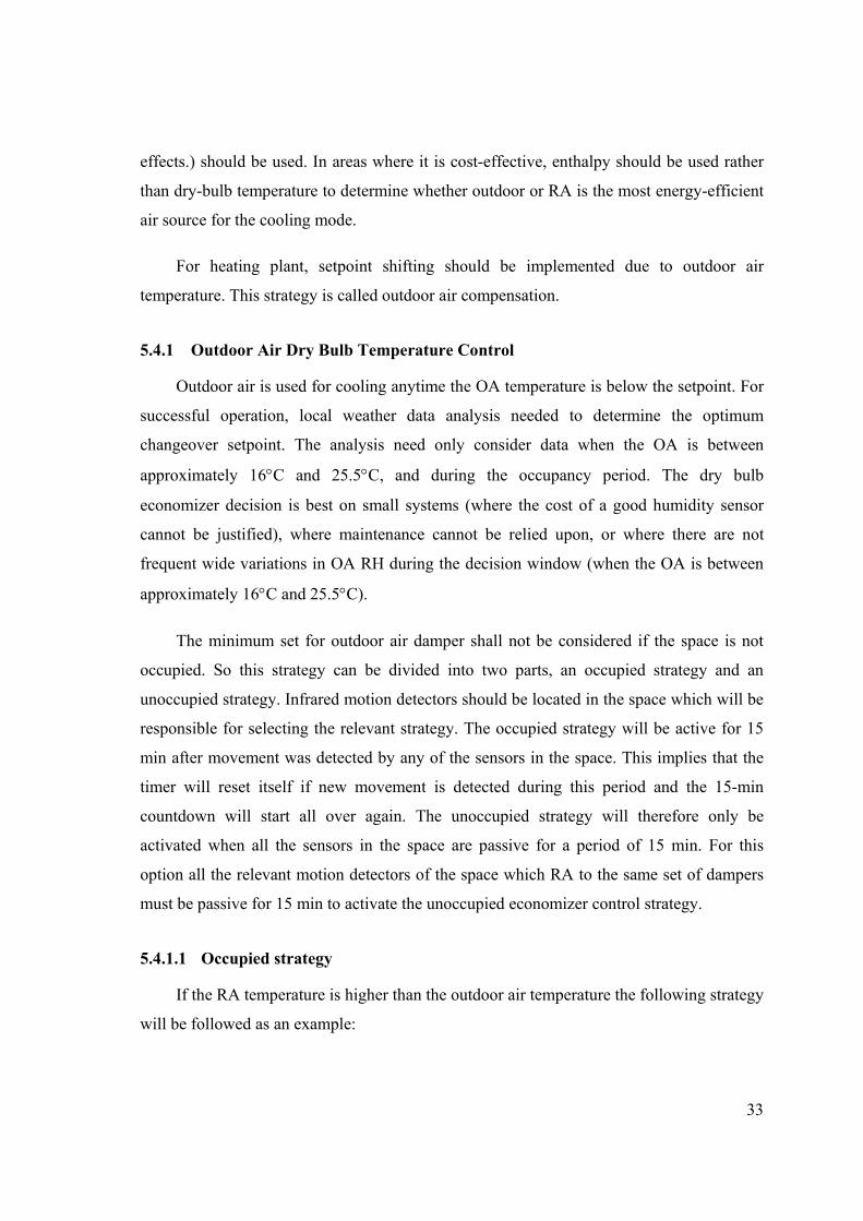
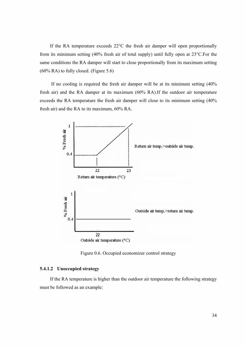
5.4.1.1 Occupied strategy

If the RA temperature is higher than the outdoor air temperature the following strategy

will be followed as an example:

34

If the RA temperature exceeds 22°C the fresh air damper will open proportionally

from its minimum setting (40% fresh air of total supply) until fully open at 23°C.For the

same conditions the RA damper will start to close proportionally from its maximum setting

(60% RA) to fully closed. (Figure 5.6)

If no cooling is required the fresh air damper will be at its minimum setting (40%

fresh air) and the RA damper at its maximum (60% RA).If the outdoor air temperature

exceeds the RA temperature the fresh air damper will close to its minimum setting (40%

fresh air) and the RA to its maximum, 60% RA.

Figure 0.6. Occupied economizer control strategy

5.4.1.2 Unoccupied strategy

If the RA temperature is higher than the outdoor air temperature the following strategy

must be followed as an example:

35

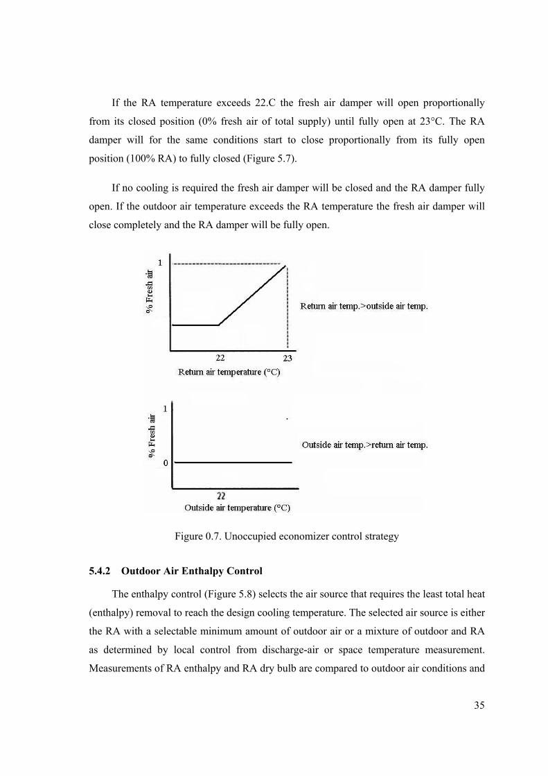
If the RA temperature exceeds 22.C the fresh air damper will open proportionally

from its closed position (0% fresh air of total supply) until fully open at 23°C. The RA

damper will for the same conditions start to close proportionally from its fully open

position (100% RA) to fully closed (Figure 5.7).

If no cooling is required the fresh air damper will be closed and the RA damper fully

open. If the outdoor air temperature exceeds the RA temperature the fresh air damper will

close completely and the RA damper will be fully open.

Figure 0.7. Unoccupied economizer control strategy

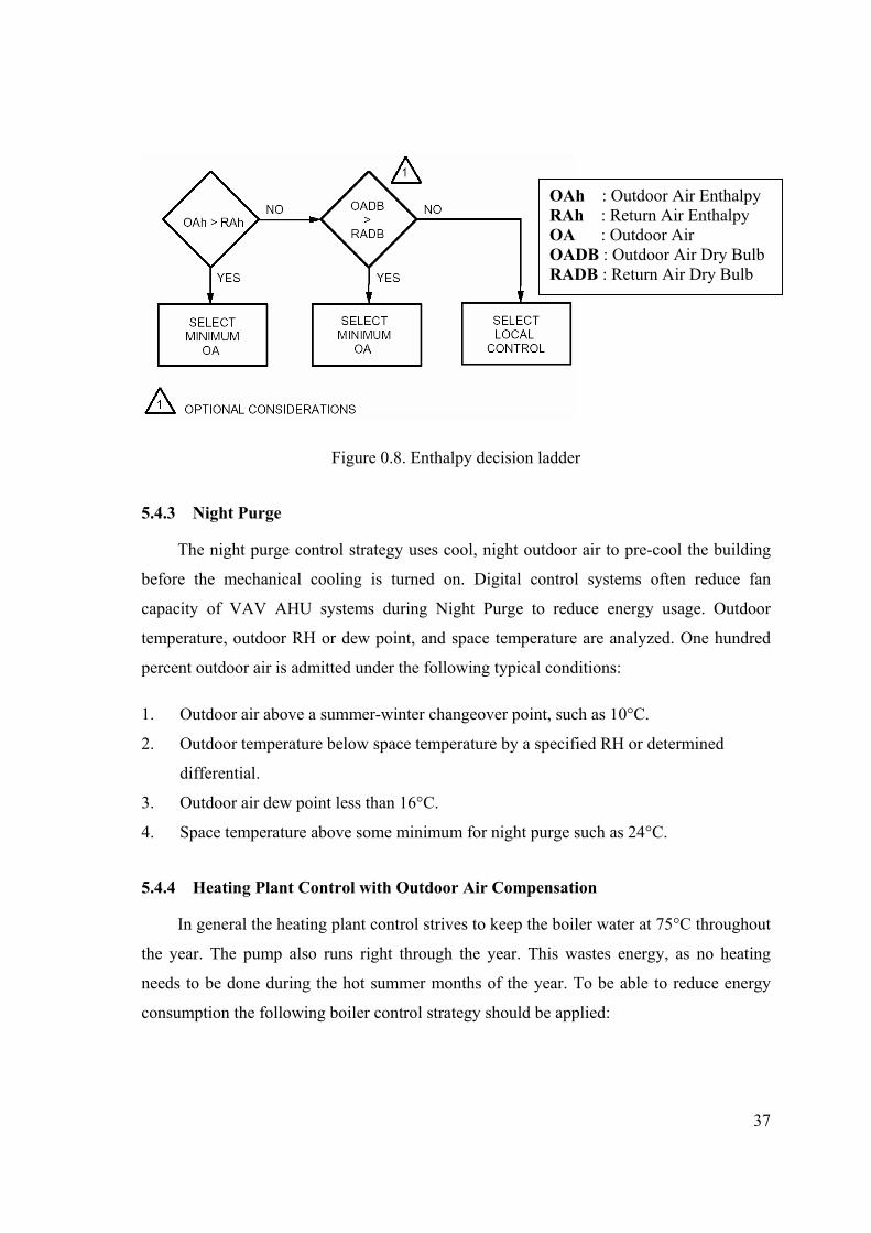
5.4.2 Outdoor Air Enthalpy Control

The enthalpy control (Figure 5.8) selects the air source that requires the least total heat

(enthalpy) removal to reach the design cooling temperature. The selected air source is either

the RA with a selectable minimum amount of outdoor air or a mixture of outdoor and RA

as determined by local control from discharge-air or space temperature measurement.

Measurements of RA enthalpy and RA dry bulb are compared to outdoor air conditions and

36

used as criteria for the air source selection. A variation of this, although not recommended,

is comparing the OA enthalpy to a constant (such as 63.96 kilojoules per kilogram of dry

air) since the controlled RA enthalpy is rather stable.

For successful operation A high quality Relative Humidity (RH) sensor with at least

3% accuracy should be selected. An estimate of the typical RA enthalpy is needed to

determine the optimum changeover setpoint. A high dry-bulb limit setpoint should be

included to prevent the enthalpy decision from bringing in air too warm for the chilled

water coil to cool down.

OA based upon an OA enthalpy calculation setpoint, except the system shall be

locked out of the economizer mode anytime the OA dry bulb (DB) is higher than 27.5°C.

Strategy shall also be provided to allow the user to switch, with an appropriate

commandable setpoint, the decision to be based upon OA dry bulb or to lock the system

into or out of the economizer mode.

Outdoor air is used for cooling (or to supplement the chilled water system) anytime

the OA enthalpy is below the economizer setpoint. OA enthalpy considers total heat and

will take advantage of warm dry low enthalpy OA and will block out cool moist OA, thus

saving more energy than a dry-bulb based economizer loop.

37

Figure 0.8. Enthalpy decision ladder

5.4.3 Night Purge

The night purge control strategy uses cool, night outdoor air to pre-cool the building

before the mechanical cooling is turned on. Digital control systems often reduce fan

capacity of VAV AHU systems during Night Purge to reduce energy usage. Outdoor

temperature, outdoor RH or dew point, and space temperature are analyzed. One hundred

percent outdoor air is admitted under the following typical conditions:

1. Outdoor air above a summer-winter changeover point, such as 10°C.

2. Outdoor temperature below space temperature by a specified RH or determined

differential.

3. Outdoor air dew point less than 16°C.

4. Space temperature above some minimum for night purge such as 24°C.

5.4.4 Heating Plant Control with Outdoor Air Compensation

In general the heating plant control strives to keep the boiler water at 75°C throughout

the year. The pump also runs right through the year. This wastes energy, as no heating

needs to be done during the hot summer months of the year. To be able to reduce energy

consumption the following boiler control strategy should be applied:

OAh : Outdoor Air Enthalpy RAh : Return Air Enthalpy OA : Outdoor Air OADB : Outdoor Air Dry Bulb RADB : Return Air Dry Bulb

38

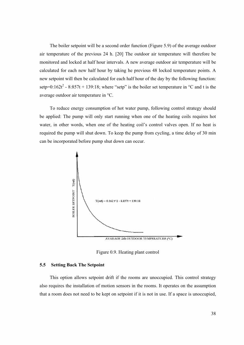
The boiler setpoint will be a second order function (Figure 5.9) of the average outdoor

air temperature of the previous 24 h. [20] The outdoor air temperature will therefore be

monitored and locked at half hour intervals. A new average outdoor air temperature will be

calculated for each new half hour by taking he previous 48 locked temperature points. A

new setpoint will then be calculated for each half hour of the day by the following function:

setp=0:162t2 - 8:857t + 139:18; where “setp” is the boiler set temperature in °C and t is the

average outdoor air temperature in °C.

To reduce energy consumption of hot water pump, following control strategy should

be applied: The pump will only start running when one of the heating coils requires hot

water, in other words, when one of the heating coil’s control valves open. If no heat is

required the pump will shut down. To keep the pump from cycling, a time delay of 30 min

can be incorporated before pump shut down can occur.

Figure 0.9. Heating plant control

5.5 Setting Back The Setpoint

This option allows setpoint drift if the rooms are unoccupied. This control strategy

also requires the installation of motion sensors in the rooms. It operates on the assumption

that a room does not need to be kept on setpoint if it is not in use. If a space is unoccupied,

39

the control will let both the cooling and heating coil setpoints to drift to hotter and colder

temperatures, respectively. (Figure 5.10) The zones will then require less cooling and

heating from the HVAC system. For the unoccupied conditions the cooling coil will be

fully open at 26°C and fully closed at 23.5°C. The heating coil will be fully open at 16.5°C

and fully closed at 18°C.

Figure 0.10. Setpoint setback control strategy

Another application for set point related strategy is to setback setpoint according to

the building operating schedule. Multistage operation technique can be implemented (3

setpoints within a day) time-of-day operating schedule. Following building operation

problem in a AHU should be considered. The 24 h operation of the building is divided into

three stages: normal setback mode (stage 1) between 19:00 and 07:00 h, start-up mode

(stage 2) between 07:00and 08:00 h and normal mode operation during the occupied period

between 08:00 and 19:00 h (stage 3). In stage 3, both thermal comfort and energy

efficiency are of prime concern, whereas in stage 1, energy efficiency is the main issue and

40

in stage 2, fast response and energy efficiency are important considerations. During a

typical day operation, the AHU system undergoes such a multistage sequence,

consequently during each stage, some of the local control loops could be turned off or

allowed to operate at fixed open loop position. For example, the outdoor air dampers could

be closed in normal hours (stage 1). After defining the performance requirements for all

three stages and appropriately choosing the local control loop tasks (closed, open loop or

closed loop), the optimization problem to be solved is to determine an optimal operating

strategy for the AHU system which meets the entire above requirement.

41

Chapter 6

CASE STUDY – OZDILEK SHOPPING CENTER (OSC)

6.1 Introduction

A case study is carried out in OSC to investigate the potential for energy savings and

to redefine control parameters for HVAC system in the building. An energy audit was

conducted according to “Washington State University Energy Program, Energy Audit

Workbook” (APPENDIX A) to determine the end-user breakdown of the energy

consumption in the shopping center. Outcome of this audit was used to identify the largest

energy consumers, which are usually also the areas with the largest energy savings

potential. The measuring of the energy utilization of the shopping center has been a very

labour intensive process.

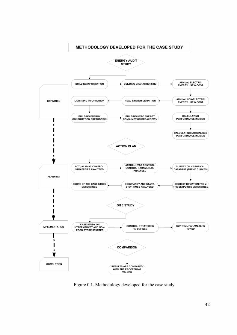
To carry out the case study systematically methodology is developed (Figure 6.1).

Case study started with a “walk through” audit to identify the energy usage of HVAC

equipment, lights and other diverse equipment. Then a detailed study was carried out to

reach regular and reliable records of energy use to understand and control the energy

management strategy. These records helped to identify changes in energy costs and

consumption. Performance evaluation of the building is determined and compared with the

accepted standards. Normalized performance indices calculated to measure building’s

efficiency better. Then an action plan was identified to implement the HVAC control

strategies to reduce energy consumption. Actual control strategies and parameters are

analyzed. Fluctuations from the setpoints are determined. New strategies and parameters

are implemented to two AHUs. Results are compared with the proceeding values.

42

ENERGY AUDITSTUDY

BUILDING INFORMATION

SURVEY ON HISTORICALDATABASE (TREND CURVES)

CALCULATING NORMALISEDPERFORMANCE INDICES

CALCULATINGPERFORMANCE INDICES

BUILDING CHARACTERISTIC ANNUAL ELECTRICENERGY USE & COST

ACTUAL HVAC CONTROLSTRATEGIES ANALYSED

ACTUAL HVAC CONTROLCONTROL PARAMETERS

ANALYSED

HIGHEST DEVIATION FROMTHE SETPOINTS DETERMINED

OCCUPANCY AND START-STOP TIMES ANALYSED

SCOPE OF THE CASE STUDYDETERMINED

CASE STUDY ONHYPERMARKET AND NON-

FOOD STORE STARTEDCONTROL STRATEGIES

RE-DEFINEDCONTROL PARAMETERS

TUNED

RESULTS ARE COMPAREDWITH THE PROCEEDING

VALUES

DEFINITION

PLANNING

IMPLEMENTATION

METHODOLOGY DEVELOPED FOR THE CASE STUDY

ANNUAL NON-ELECTRICENERGY USE & COSTHVAC SYSTEM DEFINITIONLIGHTNING INFORMATION

BUILDING HVAC ENERGYCONSUMPTION BREAKDOWN

BUILDING ENERGYCONSUMPTION BREAKDOWN

ACTION PLAN

SITE STUDY

COMPLETION

COMPARISON

Figure 0.1. Methodology developed for the case study

43

6.2 Energy Audit

To investigate energy saving potentials it is needed to analyze OSC energy usage.

Questionnaires were made and detailed investigation on electricity and Liquid Petroleum

Gas (LPG) invoices were done.

To initialize the energy audit study building information and building characteristics

were analyzed. This study included occupancy profiles and architectural locations of

HVAC zones. Then HVAC system defined and energy consumption breakdown of the

building were generated. This was very helpful to compare electricity and fossil fuel

consumptions. To be able to understand the fluctuations of energy consumption, annual

energy usage for electricity and LPG is plotted. Within this study HVAC energy

consumption is focused and various component of the HVAC energy consumption is

analyzed.

These studies are not enough to understand the building energy performance. So

performance indices are calculated and compared with the yardsticks. Then normalized

performance indices are calculated. Assessing the energy performance of this building also

allows us to:

1. Compare performance of the building with standards to suggest the potential for

energy saving in the building.

2. Compare with other buildings in an estate or group of buildings to help identify which

should be investigated first.

3. Compare with performance in previous years to monitor progress and to assess the

effects of any changes or energy saving measures.

4. Consider the energy use in more depth to help understand where energy is used and

wasted, and hence where savings are most likely to be made

The OCS has an ongoing non-systematic energy management program. These studies

are very helpful to compose the database for this energy audit. Facility management of the

shopping center is trying to coordinate the LPG usage and lightning. They also conduct

periodic maintenance to industrial refrigeration units, energy distribution panels

(preventing arc hazards), chilling units, AHU’s, water distribution pumps and boilers.

44

Based on the questionnaires the energy utilization of the shopping center is 4,360,000

kWh/year and within the current energy management studies approximate energy saving is

655.000 kWh/year (~ 15%). This saving depends on operators and should be at least 20%.

Conservation measures (retrofit) already implemented or under consideration prior to

this audit is as follows:

• Optimum start/stop depending on occupancy (assumed fixed values per days and hours). • Free outside cooling manually. • Automatic shut-down doors between heating zones. • Automatic doors in warehouse. • Warning signs to save energy for LPG usage. • Reducing heat transfer with air curtains.

6.2.1 Building Information and Characteristics

OSC is located in Inciraltı/Izmir, Turkey. The building consists of five air-conditioned

zones with approximately 16,000 m2 floor area; hypermarket, café & restaurant and

starpark (children playground) are on the ground floor (Figure 6.2), non-food store and

offices are on the first floor (Figure 6.3). The building has south-east and south-west facing

windows, with conventional glazing.

45

Figure 0.2. OSC ground floor

Figure 0.3. OSC first floor

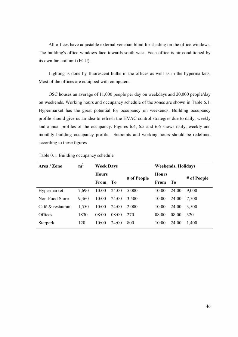
46

All offices have adjustable external venetian blind for shading on the office windows.

The building's office windows face towards south-west. Each office is air-conditioned by

its own fan coil unit (FCU).

Lighting is done by fluorescent bulbs in the offices as well as in the hypermarkets.

Most of the offices are equipped with computers.

OSC houses an average of 11,000 people per day on weekdays and 20,000 people/day

on weekends. Working hours and occupancy schedule of the zones are shown in Table 6.1.

Hypermarket has the great potential for occupancy on weekends. Building occupancy

profile should give us an idea to refresh the HVAC control strategies due to daily, weekly

and annual profiles of the occupancy. Figures 6.4, 6.5 and 6.6 shows daily, weekly and

monthly building occupancy profile. Setpoints and working hours should be redefined

according to these figures.

Table 0.1. Building occupancy schedule

Week Days Weekends, Holidays

Hours Hours

Area / Zone m2

From To # of People

From To # of People

Hypermarket 7,690 10:00 24:00 5,000 10:00 24:00 9,000

Non-Food Store 9,360 10:00 24:00 3,500 10:00 24:00 7,500

Café & restaurant 1,550 10:00 24:00 2,000 10:00 24:00 3,500

Offices 1830 08:00 08:00 270 08:00 08:00 320

Starpark 120 10:00 24:00 800 10:00 24:00 1,400

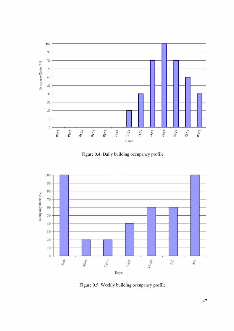
47

Figure 0.4. Daily building occupancy profile

Figure 0.5. Weekly building occupancy profile

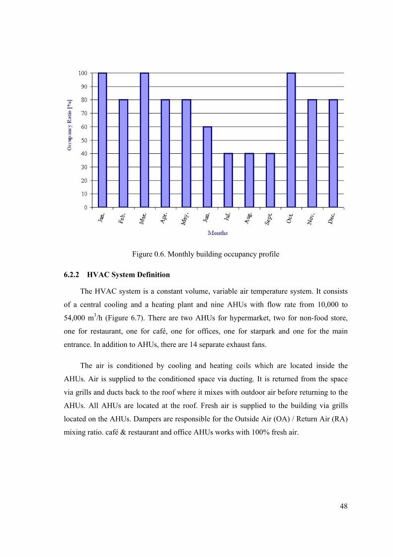
48

Figure 0.6. Monthly building occupancy profile

6.2.2 HVAC System Definition

The HVAC system is a constant volume, variable air temperature system. It consists

of a central cooling and a heating plant and nine AHUs with flow rate from 10,000 to

54,000 m3/h (Figure 6.7). There are two AHUs for hypermarket, two for non-food store,

one for restaurant, one for café, one for offices, one for starpark and one for the main

entrance. In addition to AHUs, there are 14 separate exhaust fans.

The air is conditioned by cooling and heating coils which are located inside the

AHUs. Air is supplied to the conditioned space via ducting. It is returned from the space

via grills and ducts back to the roof where it mixes with outdoor air before returning to the

AHUs. All AHUs are located at the roof. Fresh air is supplied to the building via grills

located on the AHUs. Dampers are responsible for the Outside Air (OA) / Return Air (RA)

mixing ratio. café & restaurant and office AHUs works with 100% fresh air.

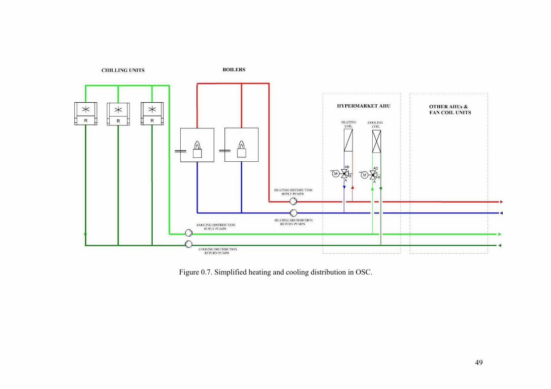
49

Figure 0.7. Simplified heating and cooling distribution in OSC.

50

The cooling of the air is done by cooling coils located inside each AHU. Digital PPI

(Proportional-Proportional-Integral) cascade controllers control the water flow through the

coils to maintain a set temperature at sensors located in the RA ducts. Three parallel,

reciprocating air-cooled chillers supply chilled water to all the cooling coils in the AHUs.

Loading and unloading of the chiller compressors maintain a set return water temperature.

Each has two compressors with a rating of 37 kW per compressor and a cooling capacity of

340 kW per chiller. Eight fans condenses the refrigerant for each cooling unit located on the

roof of the building. Chilling Units are good maintained and conventionally highly

automated. Operation profile of the chilling unit is between 09:00 and 22:00 hours on

weekdays, 09:00 and 23:00 hours on weekends, 28 weeks per year. Estimated annual hours

of operation is 2674 hrs. starting from April through November. Cooling setpoint is 6-9 °C.

13 chilled water pumps are responsible for water flow through the circuits.

Similar to the cooling coils, digital PPI cascade controllers are used to control the

heating water flow through coils to maintain a set temperature inside the air-conditioned

areas. Two fire tube-hot water type boilers which works with LPG supplies the hot water to

these coils. Boilers are maintained periodically and conventionally highly automated.

Boilers are loaded and unloaded by a step controller conventionally to keep the water inside

at a fixed set temperature 90-70°C. The boiler has a total heating capacity of 870 kW. 8 hot

water pumps are responsible for the flow through the hot water circuit.

HVAC system is equipped with BMS which controls the temperature and time

scheduled programmes. By the help of Supervisory Control and Data Acquisition

(SCADA) operator can handle the HVAC system efficiently and user friendly. 9 AHUs, 2

boilers, 16 pumps, 3 chillers and 14 exhaust fans can be controlled from the BMS which is

composed of the devices shown in Table 6.2.

51

Table 0.2. BMS equipment list

Device Quantity

PC for SCADA 1

Control panel (DDC-PLC Unit) Compact and modular, 600 data points

8

Temperature sensor Ni 1000, -30...130 °C

22

Differential pressure switch 40-300 Pa

33

3 way control valves Valves: DN 25-150 , PN16, Drives : 0..10V continuous output

22

Frost protection monitors -5...12 °C, switch. diff. : 2..6°C

11

Damper actuator 0..10V continuous output, 15Nm with spring return

22

Humidity sensor 0..10V continuous input

11

Air quality sensor 0..10V continuous input

11

6.2.3 Energy Consumption Breakdown

Outcomes of this energy audit study which was conducted according to “Washington

State University Energy Program, Energy Audit Workbook” are shown in Figures 6.8, 6.9,

6.10 and 6.11. First, general energy consumption breakdown for OCS is generated

including comparison of electricity and fossil fuel consumption (Figure 6.8). This gives an

idea of general energy usage of the building.

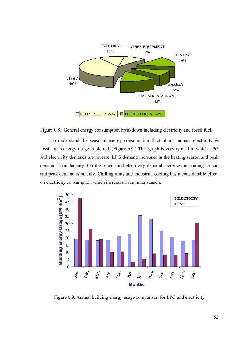
52

Figure 0.8. General energy consumption breakdown including electricity and fossil fuel.

To understand the seasonal energy consumption fluctuations, annual electricity &

fossil fuels energy usage is plotted. (Figure 6.9.) This graph is very typical in which LPG

and electricity demands are reverse. LPG demand increases in the heating season and peak

demand is on January. On the other hand electricity demand increases in cooling season

and peak demand is on July. Chilling units and industrial cooling has a considerable effect

on electricity consumption which increases in summer season.

Figure 0.9. Annual building energy usage comparison for LPG and electricity

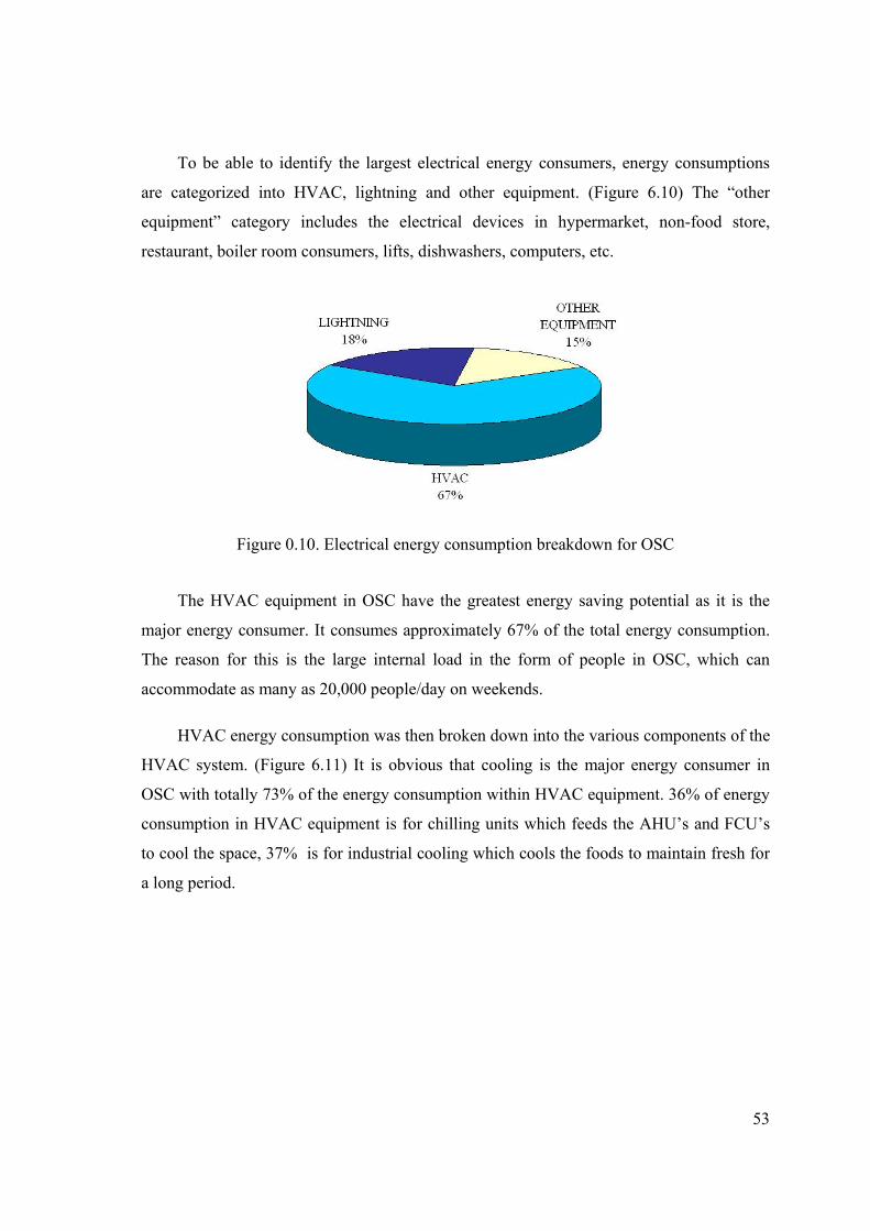
53

To be able to identify the largest electrical energy consumers, energy consumptions

are categorized into HVAC, lightning and other equipment. (Figure 6.10) The “other

equipment” category includes the electrical devices in hypermarket, non-food store,

restaurant, boiler room consumers, lifts, dishwashers, computers, etc.

Figure 0.10. Electrical energy consumption breakdown for OSC

The HVAC equipment in OSC have the greatest energy saving potential as it is the

major energy consumer. It consumes approximately 67% of the total energy consumption.

The reason for this is the large internal load in the form of people in OSC, which can

accommodate as many as 20,000 people/day on weekends.

HVAC energy consumption was then broken down into the various components of the

HVAC system. (Figure 6.11) It is obvious that cooling is the major energy consumer in

OSC with totally 73% of the energy consumption within HVAC equipment. 36% of energy

consumption in HVAC equipment is for chilling units which feeds the AHU’s and FCU’s

to cool the space, 37% is for industrial cooling which cools the foods to maintain fresh for

a long period.

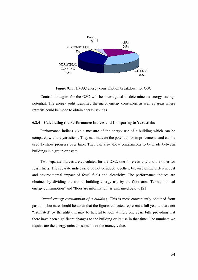
54

Figure 0.11. HVAC energy consumption breakdown for OSC

Control strategies for the OSC will be investigated to determine its energy savings

potential. The energy audit identified the major energy consumers as well as areas where

retrofits could be made to obtain energy savings.

6.2.4 Calculating the Performance Indices and Comparing to Yardsticks

Performance indices give a measure of the energy use of a building which can be

compared with the yardsticks. They can indicate the potential for improvements and can be

used to show progress over time. They can also allow comparisons to be made between

buildings in a group or estate.

Two separate indices are calculated for the OSC; one for electricity and the other for

fossil fuels. The separate indices should not be added together, because of the different cost

and environmental impact of fossil fuels and electricity. The performance indices are

obtained by dividing the annual building energy use by the floor area. Terms; “annual

energy consumption” and “floor are information” is explained below. [21]

Annual energy consumption of a building: This is most conveniently obtained from

past bills but care should be taken that the figures collected represent a full year and are not

“estimated” by the utility. It may be helpful to look at more one years bills providing that

there have been significant changes to the building or its use in that time. The numbers we

require are the energy units consumed, not the money value.

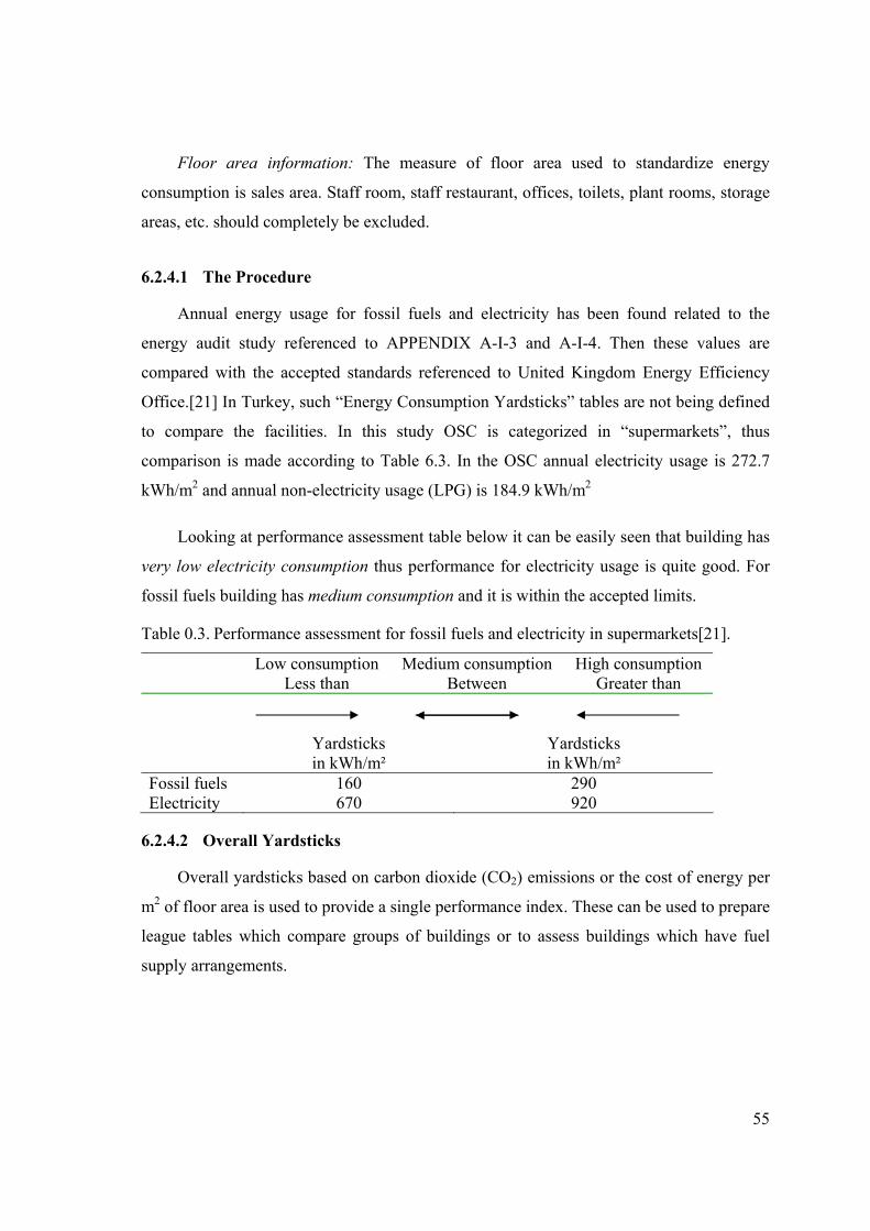
55

Floor area information: The measure of floor area used to standardize energy

consumption is sales area. Staff room, staff restaurant, offices, toilets, plant rooms, storage

areas, etc. should completely be excluded.

6.2.4.1 The Procedure

Annual energy usage for fossil fuels and electricity has been found related to the

energy audit study referenced to APPENDIX A-I-3 and A-I-4. Then these values are

compared with the accepted standards referenced to United Kingdom Energy Efficiency

Office.[21] In Turkey, such “Energy Consumption Yardsticks” tables are not being defined

to compare the facilities. In this study OSC is categorized in “supermarkets”, thus

comparison is made according to Table 6.3. In the OSC annual electricity usage is 272.7

kWh/m2 and annual non-electricity usage (LPG) is 184.9 kWh/m2

Looking at performance assessment table below it can be easily seen that building has

very low electricity consumption thus performance for electricity usage is quite good. For

fossil fuels building has medium consumption and it is within the accepted limits.

Table 0.3. Performance assessment for fossil fuels and electricity in supermarkets[21].

Low consumption Less than

Medium consumption Between

High consumption Greater than

Yardsticks Yardsticks in kWh/m² in kWh/m² Fossil fuels 160 290 Electricity 670 920

6.2.4.2 Overall Yardsticks

Overall yardsticks based on carbon dioxide (CO2) emissions or the cost of energy per

m2 of floor area is used to provide a single performance index. These can be used to prepare

league tables which compare groups of buildings or to assess buildings which have fuel

supply arrangements.

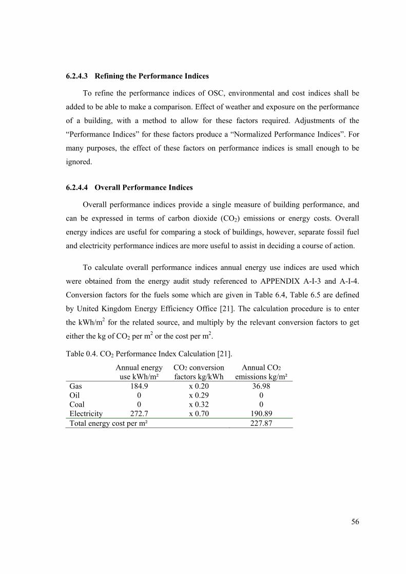
56

6.2.4.3 Refining the Performance Indices

To refine the performance indices of OSC, environmental and cost indices shall be

added to be able to make a comparison. Effect of weather and exposure on the performance

of a building, with a method to allow for these factors required. Adjustments of the

“Performance Indices” for these factors produce a “Normalized Performance Indices”. For

many purposes, the effect of these factors on performance indices is small enough to be

ignored.

6.2.4.4 Overall Performance Indices

Overall performance indices provide a single measure of building performance, and

can be expressed in terms of carbon dioxide (CO2) emissions or energy costs. Overall

energy indices are useful for comparing a stock of buildings, however, separate fossil fuel

and electricity performance indices are more useful to assist in deciding a course of action.

To calculate overall performance indices annual energy use indices are used which

were obtained from the energy audit study referenced to APPENDIX A-I-3 and A-I-4.

Conversion factors for the fuels some which are given in Table 6.4, Table 6.5 are defined

by United Kingdom Energy Efficiency Office [21]. The calculation procedure is to enter

the kWh/m2 for the related source, and multiply by the relevant conversion factors to get

either the kg of CO2 per m2 or the cost per m2.

Table 0.4. CO2 Performance Index Calculation [21].

Annual energy use kWh/m²

CO2 conversion factors kg/kWh

Annual CO2 emissions kg/m²

Gas 184.9 x 0.20 36.98 Oil 0 x 0.29 0 Coal 0 x 0.32 0 Electricity 272.7 x 0.70 190.89 Total energy cost per m² 227.87

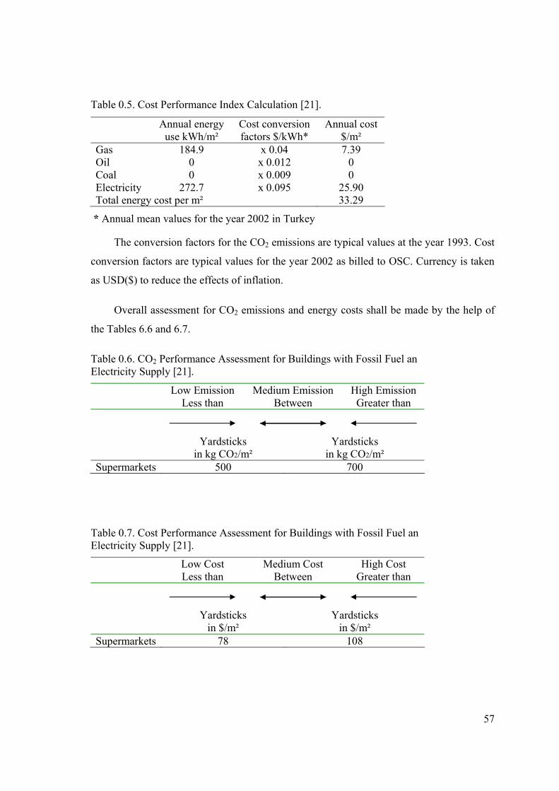
57

Table 0.5. Cost Performance Index Calculation [21].

Annual energy use kWh/m²

Cost conversion factors $/kWh*

Annual cost $/m²

Gas 184.9 x 0.04 7.39 Oil 0 x 0.012 0 Coal 0 x 0.009 0 Electricity 272.7 x 0.095 25.90 Total energy cost per m² 33.29

* Annual mean values for the year 2002 in Turkey

The conversion factors for the CO2 emissions are typical values at the year 1993. Cost

conversion factors are typical values for the year 2002 as billed to OSC. Currency is taken

as USD($) to reduce the effects of inflation.

Overall assessment for CO2 emissions and energy costs shall be made by the help of

the Tables 6.6 and 6.7.

Table 0.6. CO2 Performance Assessment for Buildings with Fossil Fuel an Electricity Supply [21].

Low Emission Less than

Medium Emission Between

High Emission Greater than

Yardsticks Yardsticks in kg CO2/m² in kg CO2/m² Supermarkets 500 700

Table 0.7. Cost Performance Assessment for Buildings with Fossil Fuel an Electricity Supply [21].

Low Cost Less than

Medium Cost Between

High Cost Greater than

Yardsticks Yardsticks in $/m² in $/m² Supermarkets 78 108

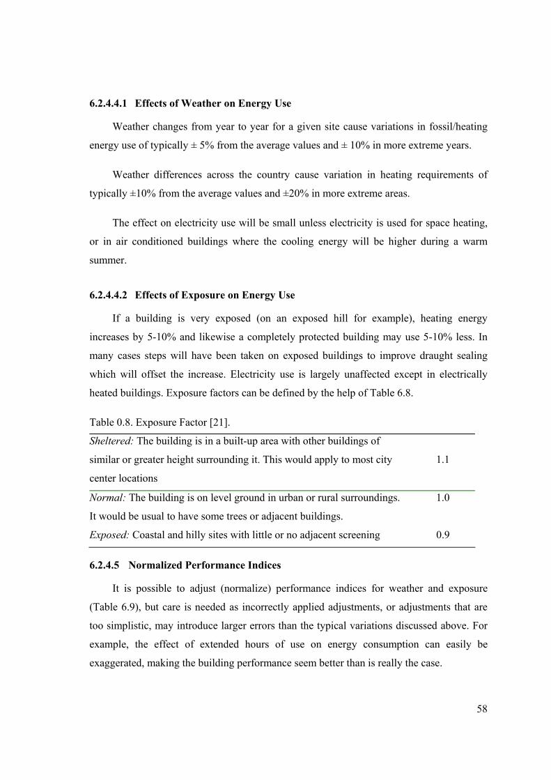
58

6.2.4.4.1 Effects of Weather on Energy Use

Weather changes from year to year for a given site cause variations in fossil/heating

energy use of typically ± 5% from the average values and ± 10% in more extreme years.

Weather differences across the country cause variation in heating requirements of

typically ±10% from the average values and ±20% in more extreme areas.

The effect on electricity use will be small unless electricity is used for space heating,

or in air conditioned buildings where the cooling energy will be higher during a warm

summer.

6.2.4.4.2 Effects of Exposure on Energy Use

If a building is very exposed (on an exposed hill for example), heating energy

increases by 5-10% and likewise a completely protected building may use 5-10% less. In

many cases steps will have been taken on exposed buildings to improve draught sealing

which will offset the increase. Electricity use is largely unaffected except in electrically

heated buildings. Exposure factors can be defined by the help of Table 6.8.

Table 0.8. Exposure Factor [21].

Sheltered: The building is in a built-up area with other buildings of

similar or greater height surrounding it. This would apply to most city

center locations

1.1

Normal: The building is on level ground in urban or rural surroundings.

It would be usual to have some trees or adjacent buildings.

1.0

Exposed: Coastal and hilly sites with little or no adjacent screening 0.9

6.2.4.5 Normalized Performance Indices

It is possible to adjust (normalize) performance indices for weather and exposure

(Table 6.9), but care is needed as incorrectly applied adjustments, or adjustments that are

too simplistic, may introduce larger errors than the typical variations discussed above. For

example, the effect of extended hours of use on energy consumption can easily be

exaggerated, making the building performance seem better than is really the case.

59

Also a normalized performance index is a better measure of a building’s efficiency

than unnormalized index; the latter shows the building’s actual performance. So a building

with a low normalized performance index, but a high performance index before adjustment,

is efficient, but since it is still a high user of energy, it may well offer good opportunities

for cost effective energy saving [21].

Performance indices shall be summarized as follows:

• Simple performance indices are for initial energy assessments. Separate performance

indices are calculated, one for fossil fuels and one for electricity use, and no

adjustments made.

• Overall performance indices, based on carbon dioxide (CO2) or cost, are normally

used when the energy supply arrangement is not typical or when a number of

buildings are to be compared. Also, you may want to know the cost or the CO2

performance for a single store.

• Normalized performance indices are used when more sensitive comparisons are

required and the effect of factors such as exposure and weather become significant.

But if you choose to normalize, be aware of introducing errors.

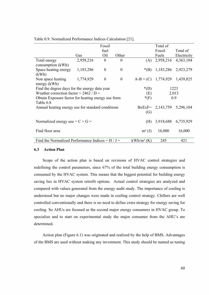
60

Table 0.9. Normalized Performance Indices Calculation [21].

Gas

Fossil fuel Oil Other

Total of Fossil Fuels

Total of Electricity

Total energy consumption (kWh)

2,958,216 0 0 (A) 2,958,216 4,363,104

Space heating energy (kWh)

1,183,286 0 0 *(B) 1,183,286 2,923,279

Non space heating energy (kWh)

1,774,929 0 0 A-B = (C) 1,774,929 1,439,825

Find the degree days for the energy data year *(D) 1223 Weather correction factor = 2462 / D = (E) 2.013 Obtain Exposure factor for heating energy use form Table 6.8

*(F) 0.9

Annual heating energy use for standard conditions BxExF= (G)

2,143,759 5,296,104

Normalized energy use = C + G = (H) 3,918,688 6,735,929 Find floor area m² (J) 16,000 16,000 Find the Normalized Performance Indices = H / J = kWh/m² (K) 245 421

6.3 Action Plan

Scope of the action plan is based on revisions of HVAC control strategies and

redefining the control parameters, since 67% of the total building energy consumption is

consumed by the HVAC system. This means that the biggest potential for building energy

saving lies in HVAC system retrofit options. Actual control strategies are analyzed and

compared with values generated from the energy audit study. The importance of cooling is

understood but no major changes were made in cooling control strategy. Chillers are well

controlled conventionally and there is no need to define extra strategy for energy saving for

cooling. So AHUs are focused as the second major energy consumers in HVAC group. To

specialize and to start on experimental study the major consumer from the AHU’s are

determined.

Action plan (Figure 6.1) was originated and realized by the help of BMS. Advantages

of the BMS are used without making any investment. This study should be named as tuning

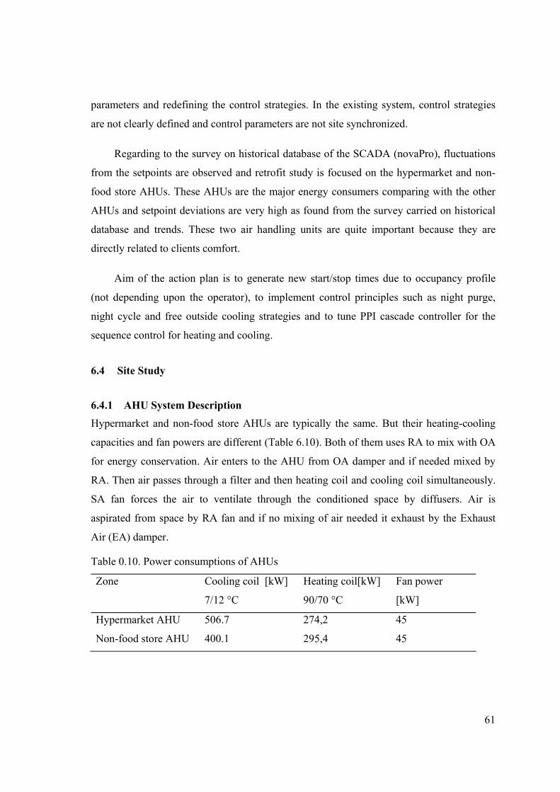
61

parameters and redefining the control strategies. In the existing system, control strategies

are not clearly defined and control parameters are not site synchronized.

Regarding to the survey on historical database of the SCADA (novaPro), fluctuations

from the setpoints are observed and retrofit study is focused on the hypermarket and non-

food store AHUs. These AHUs are the major energy consumers comparing with the other

AHUs and setpoint deviations are very high as found from the survey carried on historical

database and trends. These two air handling units are quite important because they are

directly related to clients comfort.

Aim of the action plan is to generate new start/stop times due to occupancy profile

(not depending upon the operator), to implement control principles such as night purge,

night cycle and free outside cooling strategies and to tune PPI cascade controller for the

sequence control for heating and cooling.

6.4 Site Study

6.4.1 AHU System Description Hypermarket and non-food store AHUs are typically the same. But their heating-cooling

capacities and fan powers are different (Table 6.10). Both of them uses RA to mix with OA

for energy conservation. Air enters to the AHU from OA damper and if needed mixed by

RA. Then air passes through a filter and then heating coil and cooling coil simultaneously.

SA fan forces the air to ventilate through the conditioned space by diffusers. Air is

aspirated from space by RA fan and if no mixing of air needed it exhaust by the Exhaust

Air (EA) damper.

Table 0.10. Power consumptions of AHUs

Zone Cooling coil [kW]

7/12 °C

Heating coil[kW]

90/70 °C

Fan power

[kW]

Hypermarket AHU 506.7 274,2 45

Non-food store AHU 400.1 295,4 45

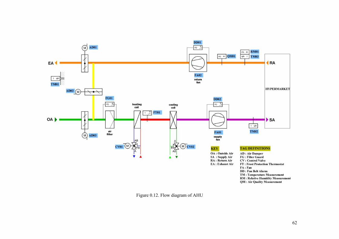
62

Figure 0.12. Flow diagram of AHU

63

6.4.2 Current Control Scenario

Supply and return fans can directly be switched on from SCADA if they are in

automatic position. These fans have interlocks in case of failure of operation which can be

observed from SCADA. AHU operates as per the sequence ‘heating coil – air dampers –

cooling coil’. The parts of the sequence are formed in the controller. The measurement for

the room-air temperature is taken in the RA duct. All control loops activate when supply

and return fans status are on. OA and EA dampers close and RA damper opens when fans

are off and modulate for temperature control when fan is on. Also heating and cooling

valves closes when fans are off.

P+PI cascade and a PI single controller is used. The supply air (SA) temperature is

measured by sensor TM02, and the room-air temperature by the RA sensor TM03. The SA

temperature is controlled by the PI auxiliary controller (control signals to CV01, CV02,

AD01,AD02 and AD03). The setpoint for the PI control loop is formed by the P main

controller, with the RA temperature as the controlled variable. The setpoint is lowered as

the RA temperature rises, and raised as it falls. The control deviation is compensated for by

adjusting the control signals to CV01, CV02, AD01, AD02 and AD03. The minimum and

maximum SA temperatures are given in the parameters of the blocks. Reversal of the

direction of operation for the control signal to AD01-AD02 and AD03 for the dampers for

heating-cooling operation in accordance with the difference between the OA temperature

and the RA temperature.

The minimum position of the fresh-air damper is set by the user interface from

SCADA view or from FBD (Function Block Diagram). FBD is a tool to parameterize and

create control logic. Return fan shall operate anytime the supply fan proves flow (via a

current sensing relay). The ventilator's fan-belt and the filter's clogging level are monitored

by differential-pressure switches. The frost-protection functions are triggered by a frost-

protection monitor which opens the heating coil in case of activation and stops supply and

return fans.

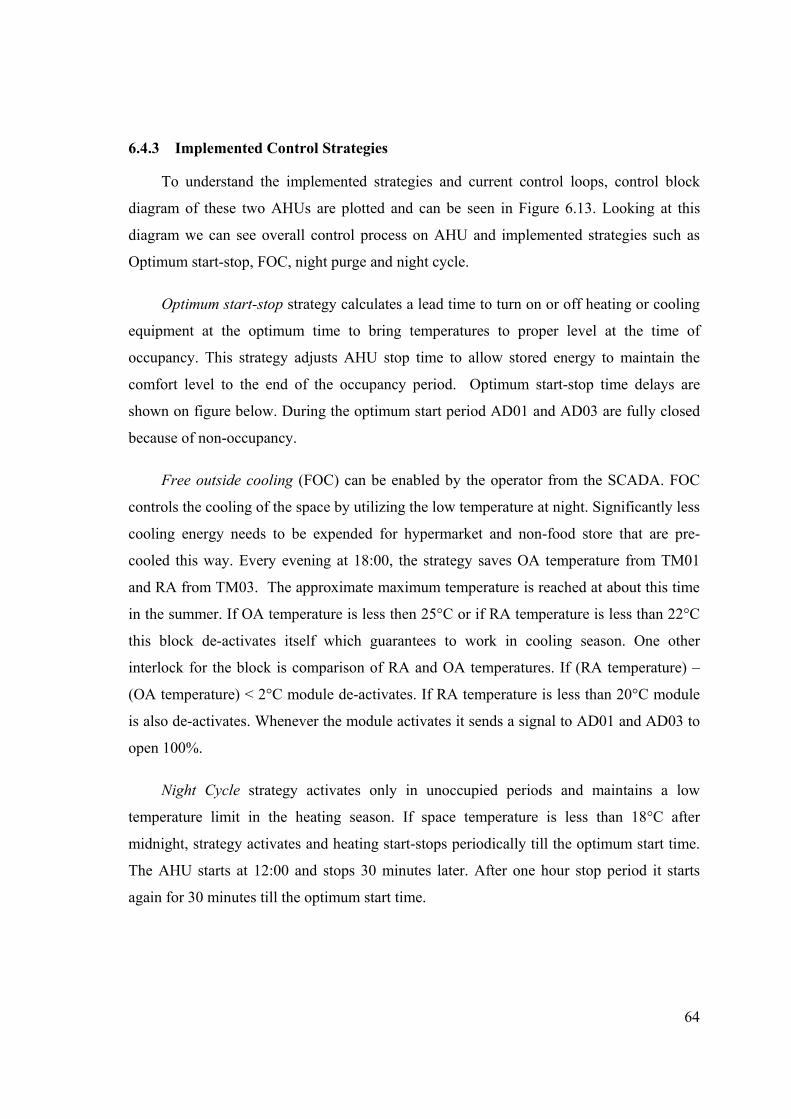
64

6.4.3 Implemented Control Strategies

To understand the implemented strategies and current control loops, control block

diagram of these two AHUs are plotted and can be seen in Figure 6.13. Looking at this

diagram we can see overall control process on AHU and implemented strategies such as

Optimum start-stop, FOC, night purge and night cycle.

Optimum start-stop strategy calculates a lead time to turn on or off heating or cooling

equipment at the optimum time to bring temperatures to proper level at the time of

occupancy. This strategy adjusts AHU stop time to allow stored energy to maintain the

comfort level to the end of the occupancy period. Optimum start-stop time delays are

shown on figure below. During the optimum start period AD01 and AD03 are fully closed

because of non-occupancy.

Free outside cooling (FOC) can be enabled by the operator from the SCADA. FOC

controls the cooling of the space by utilizing the low temperature at night. Significantly less

cooling energy needs to be expended for hypermarket and non-food store that are pre-

cooled this way. Every evening at 18:00, the strategy saves OA temperature from TM01

and RA from TM03. The approximate maximum temperature is reached at about this time

in the summer. If OA temperature is less then 25°C or if RA temperature is less than 22°C

this block de-activates itself which guarantees to work in cooling season. One other

interlock for the block is comparison of RA and OA temperatures. If (RA temperature) –

(OA temperature) < 2°C module de-activates. If RA temperature is less than 20°C module

is also de-activates. Whenever the module activates it sends a signal to AD01 and AD03 to

open 100%.

Night Cycle strategy activates only in unoccupied periods and maintains a low

temperature limit in the heating season. If space temperature is less than 18°C after

midnight, strategy activates and heating start-stops periodically till the optimum start time.

The AHU starts at 12:00 and stops 30 minutes later. After one hour stop period it starts

again for 30 minutes till the optimum start time.

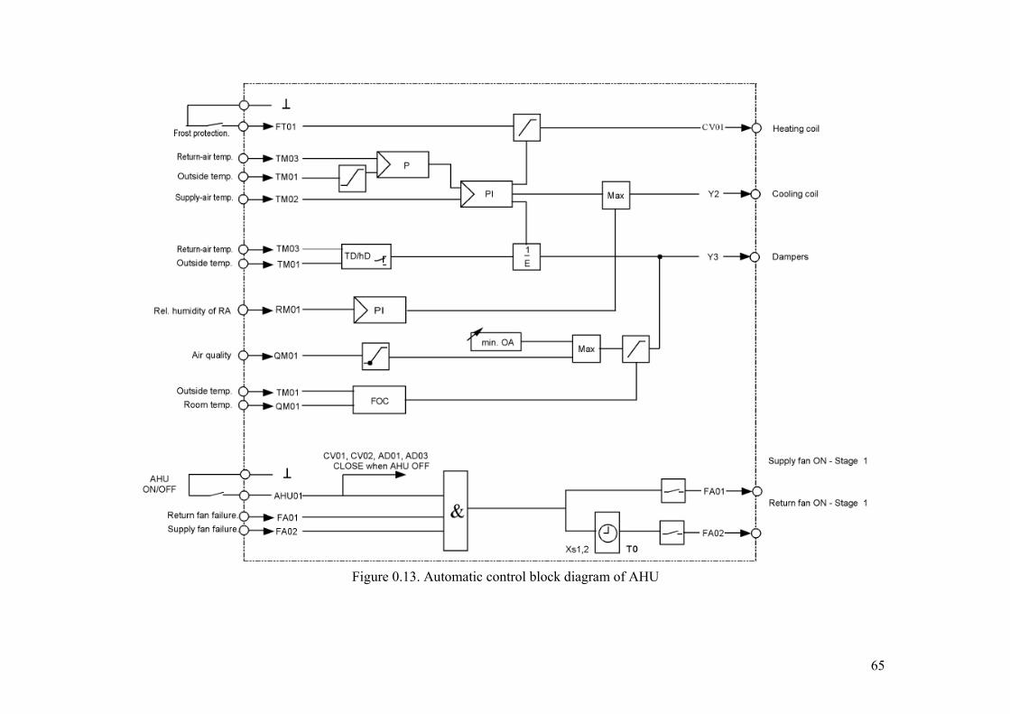
65

Figure 0.13. Automatic control block diagram of AHU

66

Night Purge strategy enables to use cool, night outdoor air to pre-cool the building

before the mechanical cooling is turned on. To activate the strategy, cooling season shall be

selected and RA temperature must be over 24°C. Also, OA dew point shall be less than

16°C.

6.4.4 Tuning control parameters

The efficiency of a control scheme to reduce energy use and to maintain comfort

largely depends on proper controller tuning. Tuning can be performed manually,

automatically with auto-tuners which have a special feature to be turned on and off by an

operator, or automatically with adaptive controllers which are self-tuning. Currently, most

commercial and institutional buildings are equipped with PID (proportional integral

derivative) controllers to keep variables, such as temperature and pressure, at predefined

setpoints which are manually tuned or with auto-tuners. In these cases, interactions between

the different control loops of the system can occur. This results in one loop being tuned to

the detriment of another.

The systematic tuning of controllers improves the performance of all controls and is

particularly important for digital control. First, the controlled process should be controlled

manually between various setpoints to evaluate the following questions:

• Is the process noisy (rapid fluctuations in controlled variable)?

• Is there appreciable hysteresis (backlash) in the actuator?

• How easy (or difficult) is it to maintain and change setpoint?

• In which operating region is the process most sensitive (highest gain)?

If the process cannot be controlled manually, the reason should be identified and

corrected before tuning the controller. Tuning selects control parameters that determine the

steady-state and transient characteristics of the control system. HVAC processes are

nonlinear, and characteristics change on a seasonal basis. Controllers tuned under one

operating condition may become unstable as conditions change. A well tuned controller

will (1) minimize the steady-state error for setpoint, (2) respond quickly to disturbances,

and (3) remain stable under all operating conditions. Tuning of proportional controller is a

67

compromise between minimizing steady-state error and maintaining margins of stability.

Proportional plus integral (PI) control minimizes this compromise because the integral

action reduces steady-state error, while the proportional term determines the controller’s

response to disturbances [22].

In the case study of OSC, tuning control parameters of the hypermarket and non-food

store AHU is focused. The process was noisy that fluctuations from the setpoints are high.

Temperature control is made by PPI cascade controller. P controller calculates a set point

for SA and SA air temperature is controlled by the PI auxiliary controller (control signals to

CV01, CV02, AD01,AD02 and AD03). Minimum and maximum limits for the SA is

determined as 16°C and 36 °C. The slope for the P main controller is 10. The setpoint for

the PI control loop is formed by the P main controller, with the RA temperature as the

controlled variable. The setpoint is lowered as the RA temperature rises, and raised as it

falls. The control deviation is compensated for by adjusting the control signals to CV01,

CV02, AD01, AD02 and AD03. Proportional band for the PI auxiliary controller is 12 and

integral time is 180 seconds. Reversal of the direction of operation of the control signal for

AD01-AD02 and AD03 is determined by heating/cooling selector which depends on OA

and RA temperature. Output signal from the PPI controller is sequenced heating coil-air

dampers-cooling coil as shown in FBD referenced to APPENDIX B

Humidity control is made by a PI block which is used only to maintain the humidity in

maximum limit. There is no humidifier in the process so only a drying by cooling coil is

defined.

Air quality control is made by a Curve-4 block. Whenever the air quality is poor the

OA damper opens to increase the quality of the conditioned space.

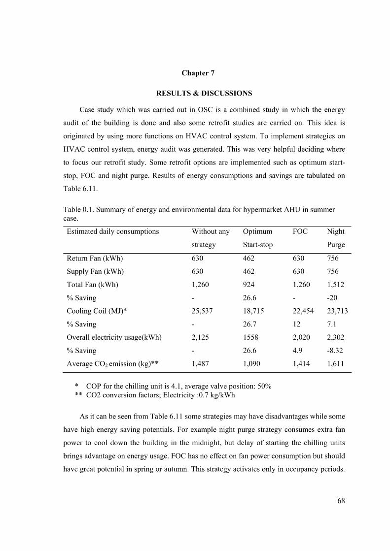
68

Chapter 7

RESULTS & DISCUSSIONS

Case study which was carried out in OSC is a combined study in which the energy

audit of the building is done and also some retrofit studies are carried on. This idea is

originated by using more functions on HVAC control system. To implement strategies on

HVAC control system, energy audit was generated. This was very helpful deciding where

to focus our retrofit study. Some retrofit options are implemented such as optimum start-

stop, FOC and night purge. Results of energy consumptions and savings are tabulated on

Table 6.11.

Table 0.1. Summary of energy and environmental data for hypermarket AHU in summer case.

Estimated daily consumptions

Without any

strategy

Optimum

Start-stop

FOC Night

Purge

Return Fan (kWh) 630 462 630 756

Supply Fan (kWh) 630 462 630 756

Total Fan (kWh) 1,260 924 1,260 1,512

% Saving - 26.6 - -20

Cooling Coil (MJ)* 25,537 18,715 22,454 23,713

% Saving - 26.7 12 7.1

Overall electricity usage(kWh) 2,125 1558 2,020 2,302

% Saving - 26.6 4.9 -8.32

Average CO2 emission (kg)** 1,487 1,090 1,414 1,611

* COP for the chilling unit is 4.1, average valve position: 50%

** CO2 conversion factors; Electricity :0.7 kg/kWh

As it can be seen from Table 6.11 some strategies may have disadvantages while some

have high energy saving potentials. For example night purge strategy consumes extra fan

power to cool down the building in the midnight, but delay of starting the chilling units

brings advantage on energy usage. FOC has no effect on fan power consumption but should

have great potential in spring or autumn. This strategy activates only in occupancy periods.

69

Optimum start-stop strategy is very important because it saves energy independent to

seasonal changes. In this study effect of night cycle strategy and heating coil energy

consumption values are not considered. These values can only be considered in the heating

season.

There are two important results for the study carried out in OSC. Comparing with the

yardsticks, the performance of the building is very good for electricity consumption and

within the accepted limits for fossil fuel (LPG) consumption. Other result is energy savings

obtained by the retrofit studies which was carried out in the hypermarket AHU.

Approximate saving for electricity usage in summer case is 22%. But studies should carry

on for every season and for long terms. Current results should not be a realistic measure of

implemented HVAC control strategies. For other AHUs and HVAC devices, such control

strategies should be implemented. This case study is done without making any investment

to the building.

OSC has an ongoing non-systematic energy management programme. Many energy

data were recorded but evaluation of these values were not considered systematically till

this study. Case study in the OSC is generated from the data of year 2002. Similar study

should be carried for the year 2003 and energy data should be evaluated and precautions

should be taken for the significant energy consumers. As a suggestion, a certified energy

manager should investigate the potentials for energy savings and should observe the energy

audit continuously.

Current BMS in the OSC should be a much more effective tool for energy

management. It needs more engineering and team-work to use more capacity of the system.

For instance, working hours of the fans, pumps etc. should be calculated and maintenance

schedules should be decided automatically. Alarm reports and trends should be printed out

regularly to understand weak parts of the HVAC system. Historical database should be

evaluated by an external programme such as MS EXCEL.

To assess the different kinds of buildings “Energy Consumption Yardsticks” tables

should be created for Turkey’s conditions. Chamber of Mechanical Engineers should

constitute a working group to form this yardstick tables.

70

Chapter 8

CONCLUSIONS

This study proves that efficient HVAC control is one of the most cost-effective

options to improve the energy efficiency of a building. The effect of changing the control

strategy is usually difficult to predict so every strategy shall be tested for every season.

Also the success of implementing efficient energy management and HVAC control is

coupled with understanding the performance of mechanical and control systems.

To initialize a case study in OSC, a methodology is developed. This methodology has

four phases: 1- Definition of building characteristics and HVAC system by conducting an

energy audit. 2- Planning of a methodology and an action plan, 3- Implementation of the

site studies. 4- Completion by comparing the results with the proceeding values.

To start a retrofit study in the OSC, energy audit study was carried out and potentials

for energy savings are investigated. Characteristics of the building and its HVAC system

understood. Within the energy audit study, performance of the building is investigated and

as a result building performance on LPG usage is medium consumption. electricity usage is

in low consumption level achieved.

Action plan was defined and hypermarket and non-food store AHUs are focused.

Control scenarios of these AHUs are deeply investigated revisions are made. Some HVAC

control strategies such as optimum start-stop, night purge, night cycle are implemented.

Control loops and parameters are tuned due to characteristics of the building. Energy

savings obtained by these retrofit studies which was carried out in the hypermarket AHU is

approximately 22% in summer case.

The importance of BMS and HVAC control strategies are understood with this study.

Authors wishes that this study leads to convince the building owners to give importance to

energy matters and HVAC control.

71

REFERENCES [1] Atilla Y, Building Energy Management A Case Study in METU Library, Master

Thesis, Mechanical Engineering, METU, (1995), p. 1. [2] Rosenfeld S.I, “Worker productivity: hidden HVAC cost”, Journal of Heating,

Ventilation and Air Conditioning, 9, (1990). p. 117. [3] Shengwei W, Ling Z, “Dynamic and real-time simulation of BMS and air-

conditioning system as a ‘living’ environment for learning / training”, Journal of Automation in Construction, 10, (2001), 487

[4] Ellis M.W, Mathews E.H, “Needs And Trends In Building And HVAC System

Design Tools”, Journal of Building and Environment, 37, (2002), 642 [5] Geller H.S, “Commercial building equipment efficiency: a state-of-the-art review”

Washington, DC, American Council for an Energy-Efficient Economy, (1998) [6] Aereboe M.B, “Energy management strategies for facility managers” SA

Refrigeration and Air conditioning, 11, (1995), 43–51 [7] Ellis M.W, “Practical evaluation and integrated simulation of building HVAC

system performance” Masters thesis, Mechanical engineering, University of Pretoria, (1996), p. 2.57–2.64

[8] Mathews E.H, Arndt D.C, Geyser M.F, ”Reducing the Energy Consumption of a

Conference Centre - A Case Study Using Software”, Journal of Building and Environment, 37, (2002), 437

[9] Zaheer-uddin M, Zheng G.R, ”Optimal control of time-scheduled heating,

ventilating and air conditioning processes in buildings”, Journal of Energy Conversion & Management, 41, (2000), 50

[10] House J.M, Smith T.F, “A system approach to optimal control for HVAC and

building systems”, ASHRAE Transactions, (1995), 101(2):647±60. [11] Kintner-Meyer M, Emery A.F, “Optimal control of an HVAC system using cold

storage and building thermal capacitance”, Journal of Energy and Buildings, (1995), 23,19±31.

[12] Mathews E.H, Arndt D.C, Geyser M.F, ”Reducing the Energy Consumption of a

Conference Centre - A Case Study Using Software”, Journal of Building and Environment, 37, (2002), 437

72

[13] The Ministry of Energy and Natural Resources – MENR web page,

www.enerji.gov.tr [14] Keskin T, Electrical Power Resources Survey and Development Administration

(EIEI) Report, (2002), p. 3. [15] Keskin T, Electrical Power Resources Survey and Development Administration

(EIEI) Report, (2002), p. 8. [16] Levermore G.J, The development and use of building management systems

(BEMSs), in BUILDING ENERGY MANAGEMENT SYSTEMS An application to heating and control, (E&FN SPON) p.6-9

[17] Hyde, A. J, “Degree-days for heating calculations”, Building Services and Environmental Engineering, (1980) 2, 6

[18] Gilligan K, Building Management System Fundamentals, in Honeywell Engineering Manual Of Automatic Control For Commercial Buildings, (Honeywell Inc., 1997), p. 185.

[19] Gilligan K, Control System Characteristics, in Honeywell Engineering Manual Of

Automatic Control For Commercial Buildings, (Honeywell Inc., 1997), p. 15. [20] Mathews E.H, Arndt D.C, Geyser M.F, ”Reducing the Energy Consumption of a

Conference Centre - A Case Study Using Software”, Journal of Building and Environment, 37, (2002), 443

[21] “Introduction to Energy Efficiency in Shops and Stores”, Booklet by Energy Efficiency Office Department of the Environment - U.K., Best Practice Programme,

(1994) [22] ASHRAE Handbook CD, Fundamentals of Control Chapter 37, Electronic Version Release 2.0, (1997), p. 20.

1

APPENDIX A

ENERGY AUDIT STUDY

Washington State University Energy Program

Energy Audit Workbook* WSUEEP98027

Table of Contents

Energy Audit Instructions

I. AUDIT FORMS

1. Building Information …………………………………………………………………….............. 2 2. Building Characteristics ………………………………………………………………… ........... 3 3. Annual Electric Use and Cost ………………………………………………………… ............. 4 4. Annual Non-Electric Energy Use and Cost ……………………………………………........... 5 5. Heating Plant ………………………………………………………………………………………6 6. HVAC Distribution System ………………………………………………………………….……7 7. Cooling Plant ………………………………………………………………………………………7 8. Domestic Hot Water ………………………………………………………………………………8 9. Food Preparation and Storage Area Equipment ………………………………………………8 10. Lighting ………………………………………………………………………………………..…9

*Note: This work book was originally prepared by the Washington State Energy Office, which is now known as the Washington State University Energy Program.

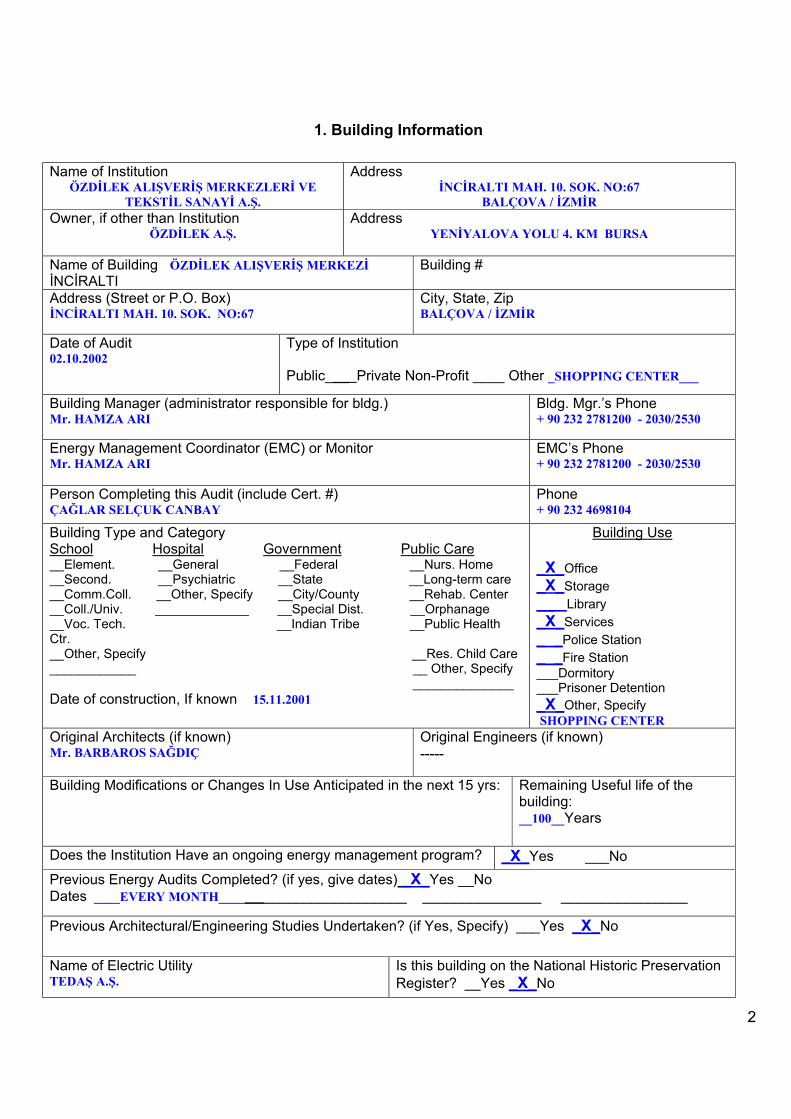
2

1. Building Information

Name of Institution ÖZDİLEK ALIŞVERİŞ MERKEZLERİ VE

TEKSTİL SANAYİ A.Ş.

Address İNCİRALTI MAH. 10. SOK. NO:67

BALÇOVA / İZMİR Owner, if other than Institution

ÖZDİLEK A.Ş. Address

YENİYALOVA YOLU 4. KM BURSA

Name of Building ÖZDİLEK ALIŞVERİŞ MERKEZİ İNCİRALTI

Building #

Address (Street or P.O. Box) İNCİRALTI MAH. 10. SOK. NO:67

City, State, Zip BALÇOVA / İZMİR

Date of Audit 02.10.2002

Type of Institution Public___ Private Non-Profit ____ Other _SHOPPING CENTER___

Building Manager (administrator responsible for bldg.) Mr. HAMZA ARI

Bldg. Mgr.’s Phone + 90 232 2781200 - 2030/2530

Energy Management Coordinator (EMC) or Monitor Mr. HAMZA ARI

EMC’s Phone + 90 232 2781200 - 2030/2530

Person Completing this Audit (include Cert. #) ÇAĞLAR SELÇUK CANBAY

Phone + 90 232 4698104

Building Type and Category School Hospital Government Public Care __Element. __General __Federal __Nurs. Home __Second. __Psychiatric __State __Long-term care __Comm.Coll. __Other, Specify __City/County __Rehab. Center __Coll./Univ. _____________ __Special Dist. __Orphanage __Voc. Tech. __Indian Tribe __Public Health Ctr. __Other, Specify __Res. Child Care ____________ __ Other, Specify ______________ Date of construction, If known 15.11.2001

Building Use _X_Office _X_Storage __ Library _X_Services _ _Police Station _ _Fire Station ___Dormitory ___Prisoner Detention _X_Other, Specify SHOPPING CENTER

Original Architects (if known) Mr. BARBAROS SAĞDIÇ

Original Engineers (if known) -----

Building Modifications or Changes In Use Anticipated in the next 15 yrs:

Remaining Useful life of the building: __100__Years

Does the Institution Have an ongoing energy management program? _X_Yes ___No Previous Energy Audits Completed? (if yes, give dates) _X_Yes __No Dates ____EVERY MONTH____ __________________ _______________ ________________

Previous Architectural/Engineering Studies Undertaken? (if Yes, Specify) ___Yes _X_No Name of Electric Utility TEDAŞ A.Ş.

Is this building on the National Historic Preservation Register? __Yes _X_No

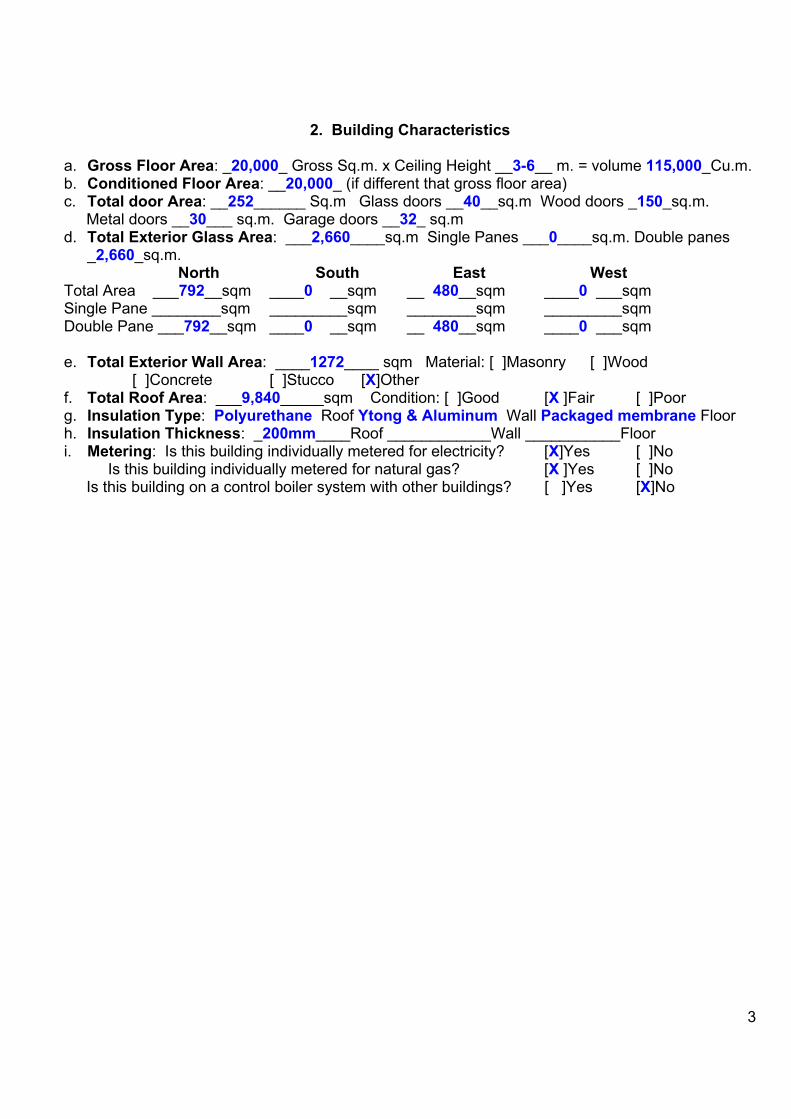
3

2. Building Characteristics

a. Gross Floor Area: _20,000_ Gross Sq.m. x Ceiling Height __3-6__ m. = volume 115,000_Cu.m. b. Conditioned Floor Area: __20,000_ (if different that gross floor area) c. Total door Area: __252______ Sq.m Glass doors __40__sq.m Wood doors _150_sq.m.

Metal doors __30___ sq.m. Garage doors __32_ sq.m d. Total Exterior Glass Area: ___2,660____sq.m Single Panes ___0____sq.m. Double panes

_2,660_sq.m. North South East West Total Area ___792__sqm ____0 __sqm __ 480__sqm ____0 ___sqm Single Pane ________sqm _________sqm ________sqm _________sqm Double Pane ___792__sqm ____0 __sqm __ 480__sqm ____0 ___sqm e. Total Exterior Wall Area: ____1272____ sqm Material: [ ]Masonry [ ]Wood

[ ]Concrete [ ]Stucco [X]Other f. Total Roof Area: ___9,840_____sqm Condition: [ ]Good [X ]Fair [ ]Poor g. Insulation Type: Polyurethane Roof Ytong & Aluminum Wall Packaged membrane Floor h. Insulation Thickness: _200mm____Roof ____________Wall ___________Floor i. Metering: Is this building individually metered for electricity? [X]Yes [ ]No

Is this building individually metered for natural gas? [X ]Yes [ ]No Is this building on a control boiler system with other buildings? [ ]Yes [X]No

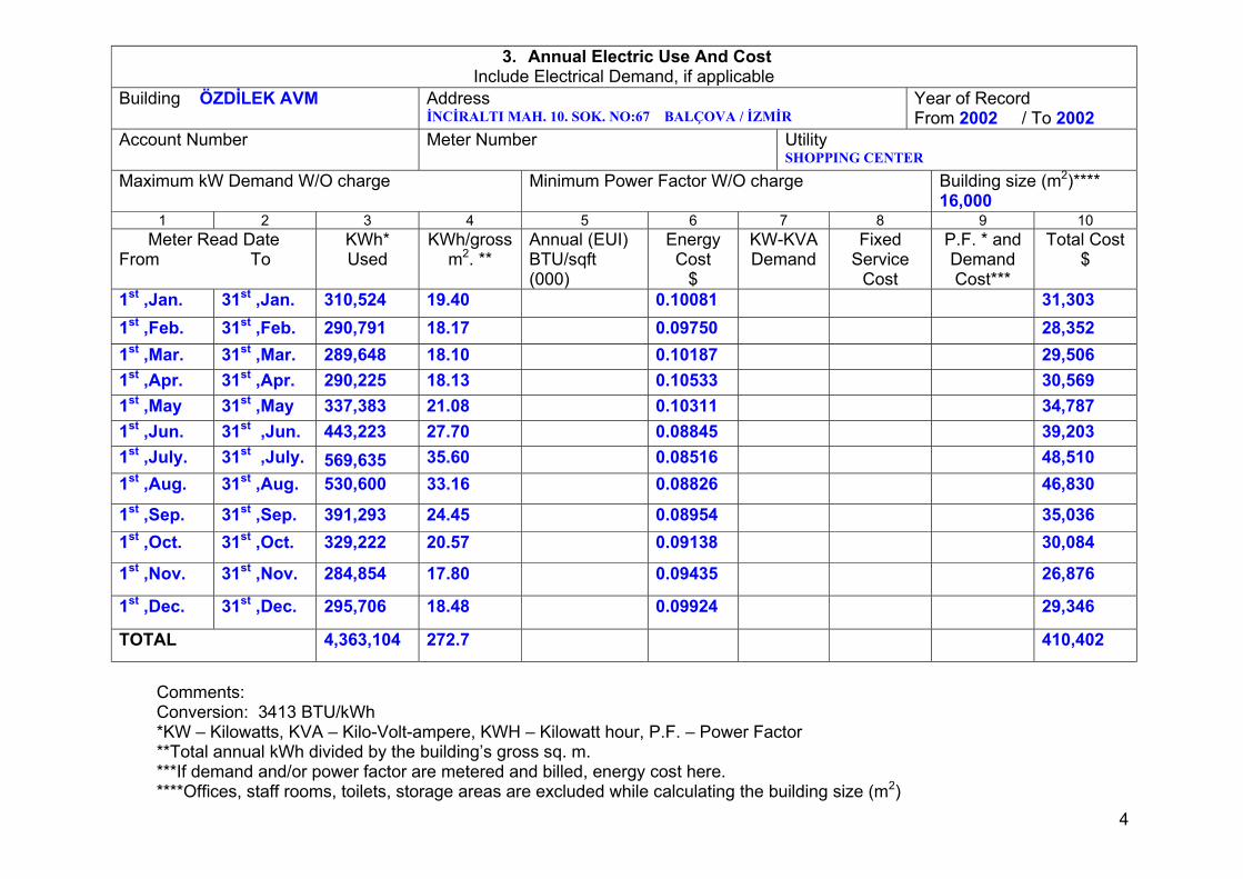
4

3. Annual Electric Use And Cost Include Electrical Demand, if applicable

Building ÖZDİLEK AVM Address İNCİRALTI MAH. 10. SOK. NO:67 BALÇOVA / İZMİR

Year of Record From 2002 / To 2002

Account Number Meter Number Utility SHOPPING CENTER

Maximum kW Demand W/O charge Minimum Power Factor W/O charge Building size (m2)**** 16,000

1 2 3 4 5 6 7 8 9 10 Meter Read Date

From To KWh* Used

KWh/gross m2. **

Annual (EUI) BTU/sqft (000)

Energy Cost

$

KW-KVA Demand

Fixed Service

Cost

P.F. * and Demand Cost***

Total Cost $

1st ,Jan. 31st ,Jan. 310,524 19.40 0.10081 31,303 1st ,Feb. 31st ,Feb. 290,791 18.17 0.09750 28,352 1st ,Mar. 31st ,Mar. 289,648 18.10 0.10187 29,506 1st ,Apr. 31st ,Apr. 290,225 18.13 0.10533 30,569 1st ,May 31st ,May 337,383 21.08 0.10311 34,787 1st ,Jun. 31st ,Jun. 443,223 27.70 0.08845 39,203 1st ,July. 31st ,July. 569,635 35.60 0.08516 48,510 1st ,Aug. 31st ,Aug. 530,600 33.16 0.08826 46,830 1st ,Sep. 31st ,Sep. 391,293 24.45 0.08954 35,036 1st ,Oct. 31st ,Oct. 329,222 20.57 0.09138 30,084

1st ,Nov. 31st ,Nov. 284,854 17.80 0.09435 26,876

1st ,Dec. 31st ,Dec. 295,706 18.48 0.09924 29,346

TOTAL 4,363,104 272.7 410,402

Comments: Conversion: 3413 BTU/kWh *KW – Kilowatts, KVA – Kilo-Volt-ampere, KWH – Kilowatt hour, P.F. – Power Factor **Total annual kWh divided by the building’s gross sq. m. ***If demand and/or power factor are metered and billed, energy cost here. ****Offices, staff rooms, toilets, storage areas are excluded while calculating the building size (m2)

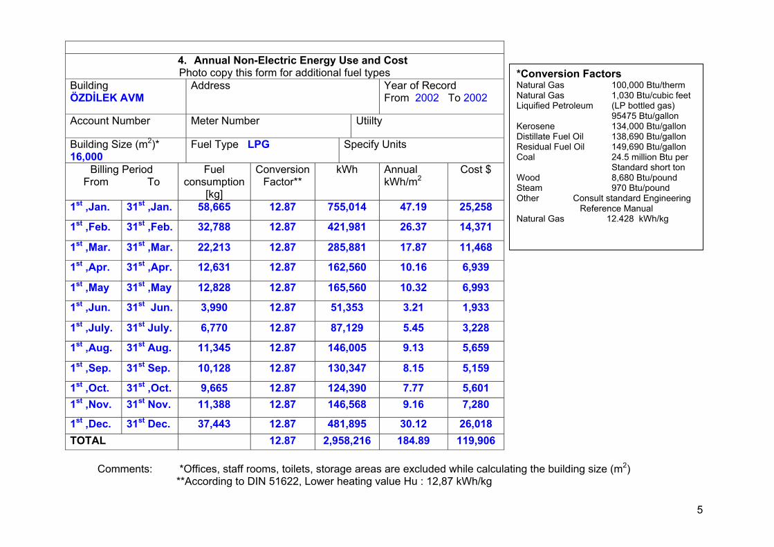
5

4. Annual Non-Electric Energy Use and Cost Photo copy this form for additional fuel types

Building ÖZDİLEK AVM

Address Year of Record From 2002 To 2002

Account Number Meter Number Utiilty

Building Size (m2)* 16,000

Fuel Type LPG Specify Units

Billing Period From To

Fuel consumption

[kg]

Conversion Factor**

kWh Annual kWh/m2

Cost $

1st ,Jan. 31st ,Jan. 58,665 12.87 755,014 47.19 25,258

1st ,Feb. 31st ,Feb. 32,788 12.87 421,981 26.37 14,371

1st ,Mar. 31st ,Mar. 22,213 12.87 285,881 17.87 11,468

1st ,Apr. 31st ,Apr. 12,631 12.87 162,560 10.16 6,939

1st ,May 31st ,May 12,828 12.87 165,560 10.32 6,993

1st ,Jun. 31st Jun. 3,990 12.87 51,353 3.21 1,933

1st ,July. 31st July. 6,770 12.87 87,129 5.45 3,228

1st ,Aug. 31st Aug. 11,345 12.87 146,005 9.13 5,659

1st ,Sep. 31st Sep. 10,128 12.87 130,347 8.15 5,159

1st ,Oct. 31st ,Oct. 9,665 12.87 124,390 7.77 5,601 1st ,Nov. 31st Nov. 11,388 12.87 146,568 9.16 7,280

1st ,Dec. 31st Dec. 37,443 12.87 481,895 30.12 26,018 TOTAL 12.87 2,958,216 184.89 119,906

Comments: *Offices, staff rooms, toilets, storage areas are excluded while calculating the building size (m2)

**According to DIN 51622, Lower heating value Hu : 12,87 kWh/kg

*Conversion Factors Natural Gas 100,000 Btu/therm Natural Gas 1,030 Btu/cubic feet Liquified Petroleum (LP bottled gas) 95475 Btu/gallon Kerosene 134,000 Btu/gallon Distillate Fuel Oil 138,690 Btu/gallon Residual Fuel Oil 149,690 Btu/gallon Coal 24.5 million Btu per Standard short ton Wood 8,680 Btu/pound Steam 970 Btu/pound Other Consult standard Engineering Reference Manual Natural Gas 12.428 kWh/kg

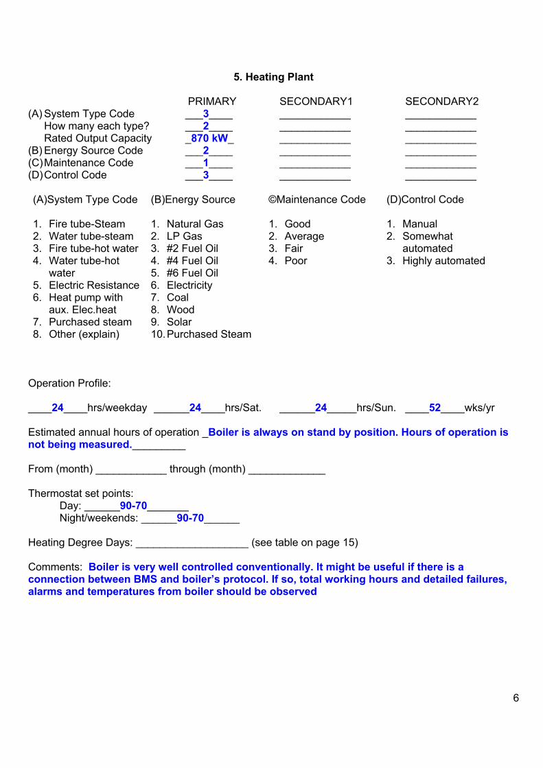
6

5. Heating Plant

PRIMARY SECONDARY1 SECONDARY2 (A) System Type Code ___3____ ____________ ____________

How many each type? ___2____ ____________ ____________ Rated Output Capacity _870 kW_ ____________ ____________

(B) Energy Source Code ___2____ ____________ ____________ (C) Maintenance Code ___1____ ____________ ____________ (D) Control Code ___3____ ____________ ____________ (A)System Type Code

(B)Energy Source ©Maintenance Code

(D)Control Code

1. Fire tube-Steam 2. Water tube-steam 3. Fire tube-hot water 4. Water tube-hot

water 5. Electric Resistance 6. Heat pump with

aux. Elec.heat 7. Purchased steam 8. Other (explain)

1. Natural Gas 2. LP Gas 3. #2 Fuel Oil 4. #4 Fuel Oil 5. #6 Fuel Oil 6. Electricity 7. Coal 8. Wood 9. Solar 10. Purchased Steam

1. Good 2. Average 3. Fair 4. Poor

1. Manual 2. Somewhat

automated 3. Highly automated

Operation Profile: ____24____hrs/weekday ______24____hrs/Sat. ______24_____hrs/Sun. ____52____wks/yr Estimated annual hours of operation _Boiler is always on stand by position. Hours of operation is not being measured._________ From (month) ____________ through (month) _____________ Thermostat set points: Day: ______90-70_______ Night/weekends: ______90-70______ Heating Degree Days: ___________________ (see table on page 15) Comments: Boiler is very well controlled conventionally. It might be useful if there is a connection between BMS and boiler’s protocol. If so, total working hours and detailed failures, alarms and temperatures from boiler should be observed

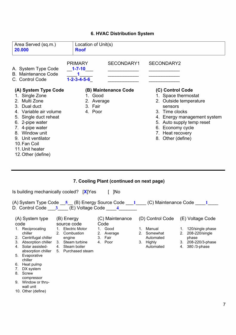
7

6. HVAC Distribution System Area Served (sq.m.) 20.000

Location of Unit(s) Roof

PRIMARY SECONDARY1 SECONDARY2 A. System Type Code __1-7-10___ ____________ ____________ B. Maintenance Code ____1_____ ____________ ____________ C. Control Code 1-2-3-4-5-6_ ____________ ____________

(A) System Type Code (B) Maintenance Code (C) Control Code 1. Single Zone 2. Multi Zone 3. Dual duct 4. Variable air volume 5. Single duct reheat 6. 2-pipe water 7. 4-pipe water 8. Window unit 9. Unit ventilator 10. Fan Coil 11. Unit heater 12. Other (define)

1. Good 2. Average 3. Fair 4. Poor

1. Space thermostat 2. Outside temperature

sensors 3. Time clocks 4. Energy management system 5. Auto supply temp reset 6. Economy cycle 7. Heat recovery 8. Other (define)

7. Cooling Plant (continued on next page) Is building mechanically cooled? [X]Yes [ ]No (A) System Type Code __5__ (B) Energy Source Code ___1____ (C) Maintenance Code ____1____ D. Control Code ___3____ (E) Voltage Code ____4_______

(A) System type code

(B) Energy source code

(C) Maintenance Code

(D) Control Code (E) Voltage Code

1. Reciprocating chiller

2. Centrifugal chiller 3. Absorption chiller 4. Solar assisted-

absorption chiller 5. Evaporative

chiller 6. Heat pulmp 7. DX system 8. Screw

compressor 9. Window or thru-

wall unit 10. Other (define)

1. Electric Motor 2. Combustion

engine 3. Steam turbine 4. Steam boiler 5. Purchased steam

1. Good 2. Average 3. Fair 4. Poor

1. Manual 2. Somewhat

Automated 3. Highly

Automated

1. 120/single phase 2. 208-220/single

phase 3. 208-220/3-phase 4. 380 /3-phase

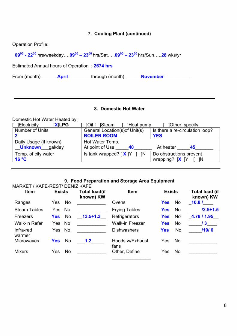
8

7. Cooling Plant (continued) Operation Profile: 0900 - 2230 hrs/weekday….0900 – 2300 hrs/Sat…..0900 – 2300 hrs/Sun…..28 wks/yr Estimated Annual hours of Operation : 2674 hrs From (month) ______April_________through (month) ______November__________

8. Domestic Hot Water Domestic Hot Water Heated by: [ ]Electricity [X]LPG [ ]Oil [ ]Steam [ ]Heat pump [ ]Other, specify

Number of Units 2

General Location(s)of Unit(s) BOILER ROOM

Is there a re-circulation loop? YES

Daily Usage (if known) __Unknown___gal/day

Hot Water Temp. At point of Use _____40_______ At heater _____45_______

Temp. of city water 16 °C

Is tank wrapped? [ X ]Y [ ]N Do obstructions prevent wrapping? [X ]Y [ ]N

9. Food Preparation and Storage Area Equipment MARKET / KAFE-REST/ DENİZ KAFE

Item Exists Total load(if known) KW

Item Exists Total load (if known) KW

Ranges Yes No ___________ Ovens Yes No _10.8 /____ Steam Tables Yes No ___________ Frying Tables Yes No _____/2.5+1.5 Freezers Yes No __13.5+1.3__ Refrigerators Yes No _4.78 / 1.95__ Walk-in Refer Yes No ___________ Walk-in Freezer Yes No _____/ 3____ Infra-red warmer

Yes No ___________ Dishwashers Yes No _____/19/ 6

Microwaves Yes No ___1.2_____ Hoods w/Exhaust fans

Yes No ___________

Mixers Yes No ___________ Other, Define _______________

Yes No ___________

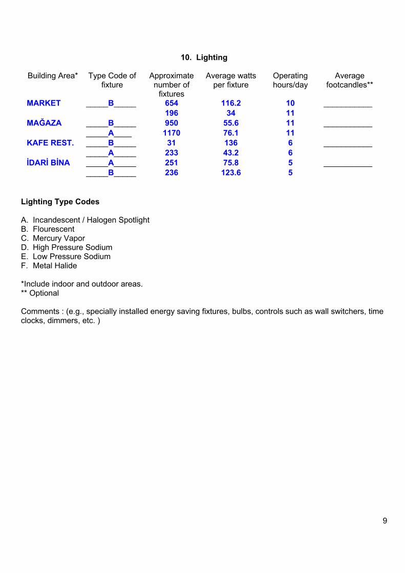
9

10. Lighting

Building Area* Type Code of fixture

Approximate number of

fixtures

Average watts per fixture

Operating hours/day

Average footcandles**

MARKET _____B_____ 654 116.2 10 ___________ 196 34 11 MAĞAZA _____B_____ 950 55.6 11 ___________ _____A____ 1170 76.1 11 KAFE REST. _____B_____ 31 136 6 ___________ _____A_____ 233 43.2 6 İDARİ BİNA _____A_____ 251 75.8 5 ___________ _____B_____ 236 123.6 5

Lighting Type Codes A. Incandescent / Halogen Spotlight B. Flourescent C. Mercury Vapor D. High Pressure Sodium E. Low Pressure Sodium F. Metal Halide *Include indoor and outdoor areas. ** Optional Comments : (e.g., specially installed energy saving fixtures, bulbs, controls such as wall switchers, time clocks, dimmers, etc. )

APPENDIX B

FUNCTION BLOCK DIAGRAM OF HYPERMARKET AHU

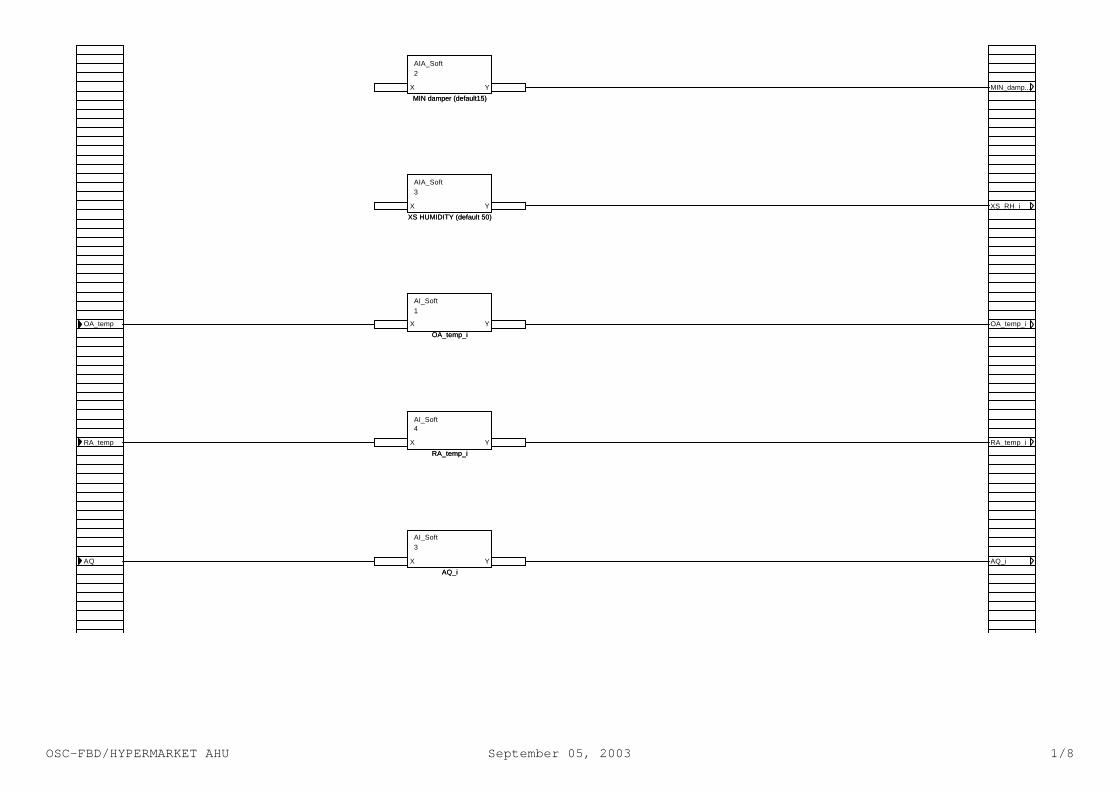
MIN_damp...

XS_RH_i

OA_temp_i

RA_temp_i

AQ_i

OA_temp

RA_temp

AQ

AIA_Soft

2

X Y

MIN damper (default15)

AIA_Soft

3

X Y

XS HUMIDITY (default 50)

AI_Soft

1

X Y

OA_temp_i

AI_Soft

4

X Y

RA_temp_i

AI_Soft

3

X Y

AQ_i

MIN_damp...

XS_RH_i

OA_temp_i

RA_temp_i

AQ_i

OA_temp

RA_temp

AQ

AIA_Soft

2

X Y

MIN damper (default15)

AIA_Soft

3

X Y

XS HUMIDITY (default 50)

AI_Soft

1

X Y

OA_temp_i

AI_Soft

4

X Y

RA_temp_i

AI_Soft

3

X Y

AQ_i

OSC-FBD/HYPERMARKET AHU September 05, 2003 1/8

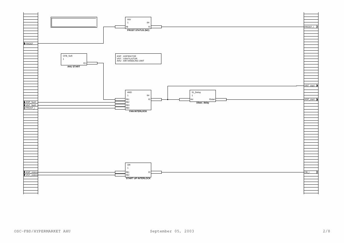
FROST_i

FROST

VNT_start

ASP_start

CB_i

ASP_fault...

VNT_fault...

FROST_i

ASP_status

VNT_status

CFB_Soft

1

fCI

AHU START

INV

641

fB fC

FROST STATUS (NC)

ASP : ASPIRATOR VNT : VANTILATOR AHU :AIR HANDLING UNIT

AND

641

fB1

fB2

fB3

fB4

fC

FAN INTERLOCK

OR

1

fB1

fB2

fC

START UP INTERLOCK

St_Delay

1

fAl fStdel

10sec. delay

FROST_i

FROST

VNT_start

ASP_start

CB_i

ASP_fault...

VNT_fault...

FROST_i

ASP_status

VNT_status

CFB_Soft

1

fCI

AHU START

INV

641

fB fC

FROST STATUS (NC)

ASP : ASPIRATOR VNT : VANTILATOR AHU :AIR HANDLING UNIT

AND

641

fB1

fB2

fB3

fB4

fC

FAN INTERLOCK

OR

1

fB1

fB2

fC

START UP INTERLOCK

St_Delay

1

fAl fStdel

10sec. delay

OSC-FBD/HYPERMARKET AHU September 05, 2003 2/8

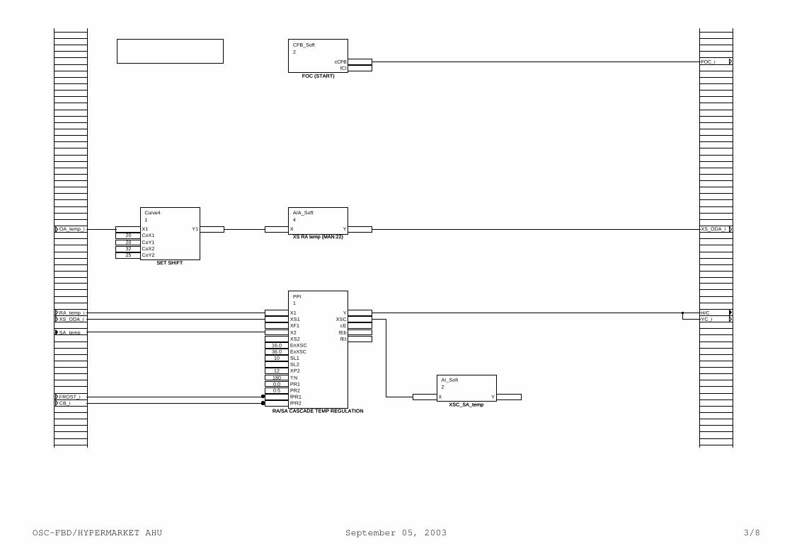
FOC_i

XS_ODA_i

H/C

YC_i

OA_temp_i

RA_temp_i

XS_ODA_i

SA_temp

FROST_i

CB_i

Curve4

1

X1

CoX120

CoY120

CoX232

CoY225

Y1

SET SHIFT

CFB_Soft

2

cCFB

fCI

FOC (START)

AIA_Soft

4

X Y

XS RA temp (MAN:22)

PPI

1

X1

XS1

XF1

X2

XS2

EnXSC16.0

ExXSC36.0

SL110

SL2

XP212

TN180

PR10.0

PR20.5

fPR1

fPR2

Y

XSC

cE

fEb

fEt

RA/SA CASCADE TEMP REGULATION

AI_Soft

2

X Y

XSC_SA_temp

FOC_i

XS_ODA_i

H/C

YC_i

OA_temp_i

RA_temp_i

XS_ODA_i

SA_temp

FROST_i

CB_i

Curve4

1

X1

CoX120

CoY120

CoX232

CoY225

Y1

SET SHIFT

CFB_Soft

2

cCFB

fCI

FOC (START)

AIA_Soft

4

X Y

XS RA temp (MAN:22)

PPI

1

X1

XS1

XF1

X2

XS2

EnXSC16.0

ExXSC36.0

SL110

SL2

XP212

TN180

PR10.0

PR20.5

fPR1

fPR2

Y

XSC

cE

fEb

fEt

RA/SA CASCADE TEMP REGULATION

AI_Soft

2

X Y

XSC_SA_temp

OSC-FBD/HYPERMARKET AHU September 05, 2003 3/8

HV

CC_i

YC_i

FROST_i

CB_i

YC_i

FROST_i

CB_i

HUMIDIFIERRH

XS_RH_i

FOC_activ...

Split_Range

2

X

CX10.52

CX21.0

CY10

CY21

fPR1

fPR2

PR10

PR20

Y

cC3P

fLV1

COOLING COIL

PID

1

X

XS

XF

En0

Ex1

SL-0.033

TN180

TV

PR10.5

Y

cE

fEb

fEt

Split_Range

1

X

CX10.0

CX20.48

CY10.0

CY21.0

fPR1

fPR2

PR11

PR20

LV10.05

Y

cC3P

fLV1

HEATING COIL

Z_Curve

1

X1

FP10.5

SL12

X2

FP20.5

SL2-2

Y1

Y2

HUMIDITY CONTROL OUTPUT

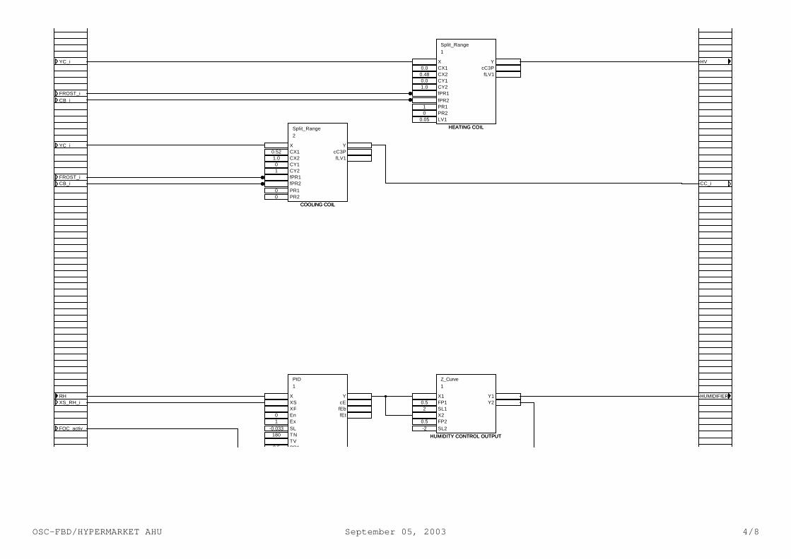
HV

CC_i

YC_i

FROST_i

CB_i

YC_i

FROST_i

CB_i

HUMIDIFIERRH

XS_RH_i

FOC_activ...

Split_Range

2

X

CX10.52

CX21.0

CY10

CY21

fPR1

fPR2

PR10

PR20

Y

cC3P

fLV1

COOLING COIL

PID

1

X

XS

XF

En0

Ex1

SL-0.033

TN180

TV

PR10.5

Y

cE

fEb

fEt

Split_Range

1

X

CX10.0

CX20.48

CY10.0

CY21.0

fPR1

fPR2

PR11

PR20

LV10.05

Y

cC3P

fLV1

HEATING COIL

Z_Curve

1

X1

FP10.5

SL12

X2

FP20.5

SL2-2

Y1

Y2

HUMIDITY CONTROL OUTPUT

OSC-FBD/HYPERMARKET AHU September 05, 2003 4/8

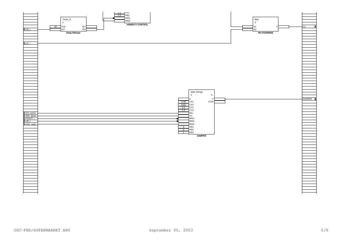
CV

DAMPER

CB_i

CC_i

H/C select

MIN_damp...

FROST_i

CB_i

FOC_activ...

Timer_A

1

Tref30

fST

fC1

fC2

Delay Release

PR10.5

PR20.5

fPR1

fPR2

HUMIDITY CONTROL

Split_Range

43

X

CX10.48

CX20.52

CY10.0

CY21.0

fSLi

XV

fPR1

fPR2

fPR3

PR10

PR20

PR31

Y

cC3P

DAMPER

Max

3

X1

X2

Y

RH OVERRIDE

CV

DAMPER

CB_i

CC_i

H/C select

MIN_damp...

FROST_i

CB_i

FOC_activ...

Timer_A

1

Tref30

fST

fC1

fC2

Delay Release

PR10.5

PR20.5

fPR1

fPR2

HUMIDITY CONTROL

Split_Range

43

X

CX10.48

CX20.52

CY10.0

CY21.0

fSLi

XV

fPR1

fPR2

fPR3

PR10

PR20

PR31

Y

cC3P

DAMPER

Max

3

X1

X2

Y

RH OVERRIDE

OSC-FBD/HYPERMARKET AHU September 05, 2003 5/8

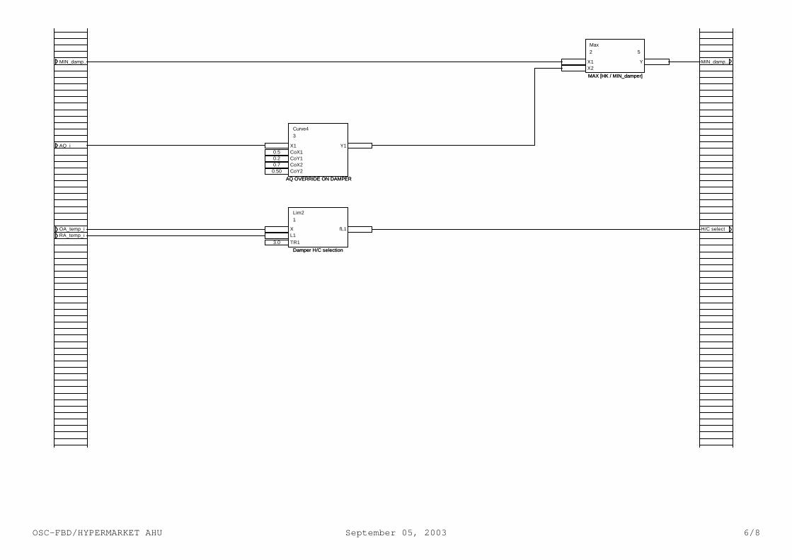
MIN_damp...

H/C select

MIN_damp...

AQ_i

OA_temp_i

RA_temp_i

Curve4

3

X1

CoX10.5

CoY10.2

CoX20.7

CoY20.50

Y1

AQ OVERRIDE ON DAMPER

Lim2

1

X

L1

TR13.0

fL1

Damper H/C selection

Max

52

X1

X2

Y

MAX [HK / MIN_damper]

MIN_damp...

H/C select

MIN_damp...

AQ_i

OA_temp_i

RA_temp_i

Curve4

3

X1

CoX10.5

CoY10.2

CoX20.7

CoY20.50

Y1

AQ OVERRIDE ON DAMPER

Lim2

1

X

L1

TR13.0

fL1

Damper H/C selection

Max

52

X1

X2

Y

MAX [HK / MIN_damper]

OSC-FBD/HYPERMARKET AHU September 05, 2003 6/8

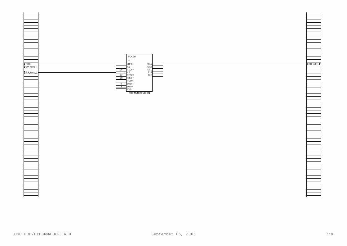
FOC_activ...FOC_i

OA_temp_i

RA_temp_i

FOCool

1

cCFB

X1

T1OFF25

X2

T2OFF22

T3OFF20

TCoff

DTOFF2

DTON2

fDIS

fDAo

fDAc

fDCL

T1F

T2F

Free Outside Cooling

FOC_activ...FOC_i

OA_temp_i

RA_temp_i

FOCool

1

cCFB

X1

T1OFF25

X2

T2OFF22

T3OFF20

TCoff

DTOFF2

DTON2

fDIS

fDAo

fDAc

fDCL

T1F

T2F

Free Outside Cooling

OSC-FBD/HYPERMARKET AHU September 05, 2003 7/8

OSC-FBD/HYPERMARKET AHU September 05, 2003 8/8